The kernel’s control-group
subsystem works well for resource management, Chris Li said at the
beginning of his memory-management-track session at the 2026 Linux Storage,
Filesystem, Memory Management, and BPF Summit. Control groups work
less well for other use cases, though. He was there to present his
proposed enhancement, called “policy groups”, that would address some of
the shortcomings that he has encountered. A consensus on how this feature
should look still seems distant, though.
AWS CloudFormation makes it easy to model and provision your cloud application infrastructure as code. CloudFormation templates can be written directly in JSON or YAML, or they can be generated by tools like the AWS Cloud Development Kit (CDK). Resources are created and managed by CloudFormation as units called Stacks.
Managing infrastructure across multiple AWS accounts and Regions is a common pattern for organizations adopting AWS best practices like multi-account strategies. However, sharing infrastructure values, such as VPC IDs, subnet configurations, or database endpoints, between stacks in different accounts or Regions has historically required multiple manual steps. Today, we’re excited to announce Fn::GetStackOutput, a new CloudFormation intrinsic function that lets you reference stack outputs across accounts and Regions directly in your CloudFormation templates and AWS CDK applications.
In this post, we walk through how Fn::GetStackOutput works in both CloudFormation and CDK, compare it with the existing Fn::ImportValue approach, and show you how to get started with practical examples.
The challenge: sharing values across accounts and Regions
When building multi-account AWS environments, teams frequently need to share infrastructure values across organizational boundaries. For example:
A networking team maintains a shared VPC in a central account, and application teams in other accounts need to reference the VPC ID.
A security team deploys shared security groups, and workload accounts need to consume them.
A platform team provisions foundational resources in one Region, and teams deploying in other Regions need those values.
Previously, you had two options:
Fn::ImportValue with exports worked well within the same account and Region but did not support cross-account or cross-Region references.
Manual approaches such as copying values between templates, passing parameters through CI/CD pipelines, or maintaining custom automation to keep values in sync.
Both approaches added operational overhead and increased the risk of configuration drift when values changed.
Introducing Fn::GetStackOutput
Fn::GetStackOutput is a new CloudFormation intrinsic function that resolves stack output references at deployment time. It provides two key advantages over the existing export/import model:
Cross-account and cross-Region support. You can reference outputs from stacks in any account and Region (within the same partition).
No exports required. You can reference any stack output directly, without the producing stack needing to declare an Export.
How it works
When CloudFormation processes a template containing Fn::GetStackOutput, it:
Identifies the referenced stack and output.
If a RoleArn is specified, assumes that role to access the target account.
Calls DescribeStacks to retrieve the output value from the specified stack and Region.
Resolves the value and continues template processing.
The function accepts four parameters:
StackName (required): The name of the stack that contains the output you want to reference.
OutputName (required): The logical ID of the output to reference. This is the key defined in the Outputs section of the referenced stack’s template, not an export name.
Region (optional): The AWS Region where the referenced stack is deployed. Defaults to the Region of the stack being created or updated.
RoleArn (optional): The ARN of an IAM role with cloudformation:DescribeStacks permissions on the referenced stack. Use this parameter when referencing a stack in a different AWS accoun
Walkthrough: four scenarios
Let’s walk through a practical example. Suppose you have a networking stack that creates a VPC:
For a more restrictive policy, scope the Resource to the specific stack ARN you want to reference.
The IAM role should be assumable by your consumer stack’s execution role. For this example, we’ll grant generic access to account 222222222222 in the trust policy:
If you’re already using Fn::ImportValue, you may be wondering when to use which. Here’s a comparison:
Fn::ImportValue:
Same account, same Region: Supported
Cross-account: Not supported
Cross-Region: Not supported
Requires explicit Export: Yes
Reference type: Strong — blocks deletion of the exporting stack
Referential integrity: Yes
Fn::GetStackOutput:
Same account, same Region: Supported
Cross-account: Supported
Cross-Region: Supported
Requires explicit Export: No
Reference type: Weak — resolved at stack create or update time
Referential integrity: No
Use Fn::ImportValue when you need strong referential integrity within the same account and Region. CloudFormation prevents you from deleting a stack that exports values consumed by other stacks.
Use Fn::GetStackOutput when you need cross-account or cross-Region references, or when you want to avoid managing explicit exports.
Understanding weak references
An important difference to understand: Fn::GetStackOutput creates weak references. This means:
The referenced stack doesn’t know it’s being referenced. Unlike exports, there is no dependency tracking between the producer and consumer stacks.
Deleting the producer stack is not blocked. If you delete the producer stack or remove the referenced output, CloudFormation does not prevent you. However, the next time the consumer stack is created or updated, the operation will fail because the reference can no longer be resolved. Because of this, deleting the producer stack may cause impact in the consumer stack.
Changes are not automatically propagated. If the output value changes in the producer stack, the consumer stack is not automatically updated. You need to run an update on the consumer stack to pick up the new value.
Best practices for weak references
Enable deletion protection on producer stacks that other stacks depend on.
Use stack policies to prevent accidental modifications to critical outputs.
Document dependencies between stacks so teams are aware of cross-stack relationships.
Scope IAM roles narrowly by restricting DescribeStacks permissions to specific stack ARNs when possible.
Using Fn::GetStackOutput with AWS CDK
CDK now uses Fn::GetStackOutput to automatically resolve cross-region and cross-account references in the same app. Previously, this required opting in through the crossRegionReferences Stack parameter.
Here’s an example of how cross-account references work in CDK:
class Provider extends Stack {
  public readonly vpc: ec2.Vpc;

  constructor(scope: Construct, id: string, props: StackProps) {
    super(scope, id, props);
    this.vpc = new ec2.Vpc(this, 'MyVpc', { maxAzs: 2 });
  }
}

interface ConsumerProps extends StackProps {
  readonly vpc: ec2.IVpc;
}

class Consumer extends Stack {
  constructor(scope: Construct, id: string, props: ConsumerProps) {
    super(scope, id, props);
    new ec2.SecurityGroup(this, 'MySG', {
      vpc: props.vpc,
      description: 'SG in Consumer using VPC from Provider',
    });
  }
}

const app = new App({
  context: {
    // choice between 'strong', 'weak', or 'both'
    '@aws-cdk/core:defaultCrossStackReferences': 'weak',
  },
});

const provider = new Provider(app, 'Provider', {
  env: { account: '111111111', region: 'us-west-2' },
});

new Consumer(app, 'Consumer', {
  env: { account: '111111111', region: 'us-west-2' },
  vpc: provider.vpc,
});
The CDK synthesizes this into a template using Fn::GetStackOutput with no additional configuration required from the user. Since this is a cross-account reference, CDK will also generate a new IAM role that can be assumed by the consumer stack.
In case of same account, cross-region, or same account and region, you can tell the CDK whether to generate strong or weak references, using the @aws-cdk/core:defaultCrossStackReferences context key. Here is how it works:
Flag=strong (default when unset):
Same account and Region: generates a Fn::ImportValue reference
Same account, cross-Region: generates an ExportWriter/ExportReader pair (legacy custom resources)
Cross-account: not possible, falls back to weak
Flag=both:
Same account and Region: generates a Fn::GetStackOutput reference and an Export, but not Fn::ImportValue
Same account, cross-Region: generates a Fn::GetStackOutput reference and an ExportWriter, but not the ExportReader
Cross-account: generates a Fn::GetStackOutput reference and a cross-account IAM role
Flag=weak:
Same account and Region: generates a Fn::GetStackOutput reference
Same account, cross-Region: generates a Fn::GetStackOutput reference
Cross-account: generates a Fn::GetStackOutput reference and a cross-account IAM role
You can also resolve cross-region or cross-account references between stacks in different CDK Applications explicitly using the Fn.getStackOutput() method. For more information, see the CDK documentation.
For cross-account references, create an IAM role in the producer account with cloudformation:DescribeStacks permissions.
Add the function to your template. Use the Fn::GetStackOutput syntax with the appropriate parameters.
Deploy your stack. CloudFormation resolves the reference during the create or update operation.
Conclusion
Fn::GetStackOutput simplifies multi-account and multi-Region infrastructure management by enabling direct references between stacks without requiring explicit exports or custom workarounds. Whether you’re using CloudFormation templates directly or building with the AWS CDK, this new capability reduces operational overhead and the risk of configuration drift across your organization.
This feature is available in all AWS Regions where CloudFormation is supported. To learn more, visit the Fn::GetStackOutput documentation in the CloudFormation Template Reference Guide.
Блокадата на Ормузкия проток, наложена от администрацията на американския президент Доналд Тръмп, и ограничаването на военните действия в Близкия изток бяха разтълкувани от много експерти като крачка напред към постигането на мир в региона. Това спокойствие обаче далеч не трябва да се приема оптимистично, тъй като твърдата сила и оръжията далеч не са най-ефективният начин да ескалираш един конфликт през XXI век.
След продължителната размяна на удари между Вашингтон и Техеран политиците от двете страни явно разбраха, че ескалацията между тях лесно ще трансформира конфликта в криза. Казано с други думи, вместо да контролират ситуацията, тя ще започне да ги контролира, което може да доведе до пълномащабна война в Близкия изток, в която ще се включат и арабските държави. За това осъзнаване допринесе и позицията на много европейски държави, които отказаха да подкрепят САЩ в ударите им с аргументите, че тази война не е война на Европа и че НАТО е отбранителен алианс, който не може да бъде използван като инструмент в американската външна политика.
В тези условия администрацията на Тръмп реши да вкара в действие план Б – да разшири конфликта икономически и енергийно, като в същото време го ограничи до обхвата му към момента. Това би могло да даде на американските съюзници в региона глътка въздух, като същевременно не би позволило на Иран да се прегрупира и да засили позициите си.
Каква обаче е истинската дилема на страните в конфликта и какъв е истинският залог? В този материал ще се опитаме да погледнем отвъд шаблонните изказвания на лидерите, към реалната награда, която ще получи победителят във войната.
Американската дилема в Ормузкия проток
В първите часове след началото на операция „Епична ярост“ в международната общност се очертаха две основни гледни точки за ударите, които Вашингтон реши да нанесе върху ядрената инфраструктура на Ислямска република Иран. Много европейски държави, включително съюзници от НАТО, както и доста от арабските държави застанаха на позицията, че интервенцията на Тръмп има нападателен характер, като същевременно отчетоха и опасността Иран да се сдобие с ядрени оръжия за военни цели.
Най-категорични бяха Италия и Испания, които отказаха достъп на американците до военните си бази, от които САЩ възнамеряваха да нанесат ударите си срещу Техеран. Арабските регионални сили, като Саудитска Арабия и Катар, бяха малко по-сдържани в позицията си, тъй като крахът на шиитската империя би бил добре дошъл за сунитските държави в региона. Но когато конфликтът заплаши да излезе извън границите на Иран, Рияд също отказа достъп на САЩ до собствените им бази, разположени на Арабския полуостров. Тази огромна липса на консенсус сред американските съюзници и партньори, към която по-късно дискретно, но знаково се присъединиха Германия и Кувейт, не позволи на Вашингтон да разгърне сухопътна операция в региона, което накара Тръмп да заложи на морска блокада.
Начело на втория лагер – държави, които подкрепиха САЩ, застанаха Полша, Чехия, Албания, Косово, Република Северна Македония, Литва, Латвия, България и Унгария, които осъдиха иранската ядрена програма, като нашата страна дори предостави въздушното си пространство за рутинни учения на НАТО. Встрани от Израел, който е пряк участник в конфликта, влиятелни съюзници от Алианса, като Великобритания и Турция, осъдиха атаките на САЩ на думи, но в същото време спомогнаха за действията на Америка, особено Лондон, който предостави впоследствие базите си за удари срещу Техеран. Най-хитра от всички беше позицията на Турция, която усилено критикуваше американския президент, а в същото време играеше ролята на мълчалив брокер между двете страни.
Дилемата на САЩ беше доста сложна. Съгласно т.нар. QME акт, приет през 2008 г. от Конгреса, Вашингтон беше длъжен да помогне на Израел, тъй като нормалното съществуване на държавата беше поставено на карта поради продължаващата регионална ескалация на напрежението в Близкия изток след терористичните атентати от 7 октомври 2023. В същото време Тръмп трябваше да защити икономическите интереси на Америка, сериозно пострадали от търговската война с Китай – цел, която не беше постигната поради огромната цена, плащана от Вашингтон във войната с Иран.
На фона на тази картина ударът на САЩ беше изпреварващ дотолкова, доколкото целеше унищожаването на иранската ядрена програма и защитата на Израел. И тук се появи разделителната линия между съюзниците – Вашингтон виждаше целите на операцията като постигнати, а в Израел заговориха за смяна на режима в Иран.
Тръмп вероятно си е дал сметка, че ако САЩ започнат сухопътна операция в посока Техеран, „Епична ярост“ще се превърне от изпреварващ удар в класическа стратегия за смяна на режим, подобно на американските намеси в Ирак и Афганистан след 11 септември. Казано с други думи, САЩ трябваше да избират между „втори Афганистан“, въвличането на арабските партньори във войната и влошаването на отношенията с Израел. В тези условия американската администрация се насочи към единственото възможно решение, което да внесе баланс в ситуацията – блокада на Ормузкия проток. Съвсем отделен е въпросът, че цената за това решение постави на карта ключово важни американски позиции в световната икономика.
Дилемата на Иран и Израел
Парадоксалното е, че ако за САЩ дилемата в Близкия изток е по-скоро критично важна, то за Иран и Израел тя е екзистенциална. Разликата между двете е, че с критично важните си национални интереси можеш да правиш все пак компромис, докато с екзистенциалните няма как – или воюваш, или те завладяват. За Израел ядрено въоръжен Иран, мечтаещ от десетилетия за унищожаването на израелската държава, означава повишено ниво на внимание, което като предизвикателство за националната сигурност от такъв мащаб няма как да бъде сдържано с конвенционални инструменти.
За Иран развитието на ядрената му програма означава и изграждане на способности, които биха могли да му дадат власт, каквато никой от съседите му не притежава: оръжия, достигащи първо Европа, а в рамките на следващото десетилетие – и САЩ. Без ядрено оръжие оцеляването на режима на аятоласите (или поне на това, което е останало от него) е под въпрос. А по правило авторитарните режими винаги се грижат преди всичко за собствената си лидерска сигурност, а едва след това за живота на цивилните си граждани.
Макар и да изглежда като самотен вълк, Иран далеч не е сам в желанието си да детронира Америка в Близкия изток. Зад него са Русия и Китай, които виждат в Техеран силен лост за проектиране на сила в региона. Проблемът в тези сметки е, че много често Москва и Техеран си представят ядрен Иран като Северна Корея, която продължава да развива нападателните си способности, без да се съобразява със статуквото в Североизточна Азия. Но за Пхенян, или по-точно за династията Ким, врагът винаги е бил един – Южна Корея. Америка остава големият противник, но близостта на Китай и икономическата зависимост на Сеул от Пекин не позволява на Ким Чен Ун и приближените му да разгърнат програмата си до такава степен, че да променят статуквото в Азия.
Най-важният фактор, който обаче слабо се отчита от съюзниците на Иран, е религиозно-политическият. Точно тук е редно да отбележим, че иранската доктрина няма нищо общо с класическата интерпретация в шиитския ислям. Велаят-е факих – доктрината на Рухола Хомейни – се отрича от много шиитски учени като политическа интерпретация на исляма, сходна с тази на салафизма. Това прави Техеран много по-рисков актьор от Северна Корея – затворена държава, чиято идеология не се е променяла от Втората световна война насам.
Израел, от друга страна, се намира в ситуация, в която оцеляването му е поставено на карта за пръв път от неговото създаване. Иран най-сетне е на път да се сдобие с оръжие, което може да порази Израел фатално – факт, за който свидетелстват много израелски военни учени и висши офицери. Израел гледа на Иран като на много по-голяма заплаха от останалите арабски държави, защото все пак има положителен исторически опит с Египет, Саудитска Арабия и Обединените арабски емирства (ОАЕ). Макар и критични към Израел, тези държави винаги са отчитали реалистично цената на мирното съжителство в Близкия изток и необходимостта от баланс на силите, който да предотврати ескалация. Иран е изключение и тъкмо затова голяма част от арабските държави скрито подкрепят САЩ във военната им операция.
Първата причина за тази скрита подкрепа е религиозно-политическата доктрина, за която вече стана въпрос. Втората е, че ако нещо се случи с Израел, следващата държава в списъка е Саудитска Арабия, а след нея – Катар, ОАЕ и Египет. Ето защо за арабските държави дори и ядрено въоръженият Израел може да се окаже много по-приемлив съсед, отколкото Иран, който лесно би се превърнал в източник на напрежение, особено ако оръжията му попаднат в ръцете на трансграничните терористични мрежи. Единственото изключение от това правило е Турция. Тя обмисля разработването на свой ядрен потенциал – ход, който би се превърнал в истински кошмар за Техеран, тъй като тогава той ще се окаже притиснат между две ядрени държави.
Ако САЩ победят в тази война, тяхното глобално превъзходство ще бъде съхранено за следващото десетилетие, тъй като пръстенът, който Тръмп се опитва да заключи между Гренландия и Иран, ще е частично завършен. За да стане това обаче, Америка ще има нужда от съюзниците си и от едно голямо „да“ от страна на арабските държави. На този етап подобен хоризонт изглежда нереалистичен и причината са идеологическите борби между политиците в Европа и в Америка – когато от едната страна на океана управляват либерали, а от другата консерватори, позициите им водят до конфликти.
Ето защо американската администрация ще заложи на стратегията на задушаването, която вече виждаме да се осъществява с Русия във войната с Украйна. В контекста на Иран вероятно Вашингтон няма да се стреми непременно към бърза смяна на режима или към тотална война, а към продължителен натиск, който постепенно да отслабва способността на Техеран да проектира влияние. Дали обаче тази ситуация може да сработи в Близкия изток и доколко Европа ще е готова да подкрепя съюзниците на САЩ в региона, както например подкрепя Украйна, също е под въпрос.
Едно стратегическо поражение за Вашингтон в Близкия изток би означавало преди всичко победа за Москва и Пекин. В тези условия Русия и Китай могат да си позволят да диктуват баланса на силите в региона, но за кратко, тъй като в момента, в който Иран завърши ядрената си програма, едва ли ще се съобразява с това, което му се спуска отгоре.
Бедата е, че в момента Техеран се управлява от военни, които – както и арабските държави добре осъзнават – са едни от най-големите съюзници на терористите. В обозримо бъдеще това създава опасност ядрени технологии да попаднат в ръцете на недържавни актьори, чиято идеология не съвпада с рационалното мислене на държавните. До момента в научния дебат няма трудове, посветени на този въпрос, но повечето анализатори от ерата на Студената война приемат, че такова развитие на нещата може да доведе до ядрена дилема на сигурността в Близкия изток.
Дали обаче е реалистичен и мирен сценарий за региона? Това обикновено се случва, ако страните седнат на една маса и се разберат. Диалогът е основна предпоставка за постигането на консенсус, а желание за такъв диалог липсва. Едно е сигурно – икономическите последици от конфликта ще са изключително трудни за преодоляване и могат да доведат до нова глобална икономическа криза.
В тези условия България поне има късмета, че се разплаща с основна резервна валута, което би спомогнало Европейската централна банка да регулира ценовата стабилност у нас, ако нещо се обърка.
От друга страна, не можем да отречем, че новото негласно разделение в НАТО и ЕС вече е факт – разделение на американски лагер, обхващащ Централна и Източна Европа, и на западноевропейски блок. Тъжното е, че тези разделения не са геополитически, а зависят от идеологическите лагери, към които принадлежат респективно европейските и американските елити. Единственият изход е мащабна реформа в Алианса и в Общността – реформа, която ще промени значително НАТО и ЕС от вида, в който ги познаваме.
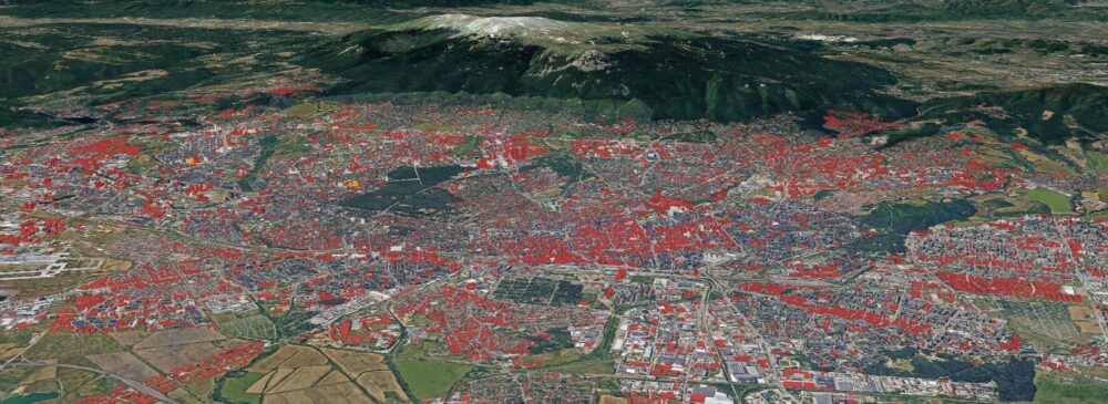
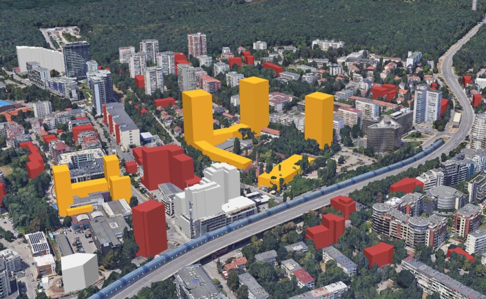
В процеса на обновяване на данните от потенциалното застрояване в 3D картата попадам на доста документи и планове. От януари 2025-та насам добавих или промених над 8600 сгради на база визи за проектиране, искания за ПУП и градоустройствени заповеди. Една такава промяна е за въведения първо през 2024-та на картата блок на ул. Шишман, за който през март имаше входирано искане за нов ПУП с по-голяма височина. Стана известен в последните дни след като публикувах визуализация и има вече петиция срещу плановете най-вече на Българската православна църква. Разбра се, че Столична община е разглеждала от самото начало сериозно искането и търси начин да се запази облика на улицата и културното наследство. Район Сердика публикува също отрицателното си становище. Няма издадено разрешение, но е важно да се спомене, че действията на Министерството на културата са ключови в този процес.
Всички сгради на картата са на база такива документи или на нанесените вече скици в слоевете Застрояване в портала на общината. Обясних подробно процеса и отговорих на критиките за тази методология.
Зеленина в рекламите, бетон в експлоатация
Излиза обаче още доста информация. Особено, ако обръщате повече внимание на темата, ще бъдете залети в социалните мрежи от реклами на нови проекти за сгради. Всички са плувнали в зеленина, с обещания за чист въздух, широки пространства и природа наоколо. Разбира се, практически никога реалността не наподобява тези картинки. Често си личи още от рано, например при снимките пуснати от кмета на Младост.
В някои случаи обаче чрез такива реклами научаваме за плановете на инвеститори за големи проекти, за които не само няма още разрешение за строеж, но не е искано промяна на ПУП дори или задействан какъвто и да е процес. Някои са по-скоро мечти, а други е ясно че ще се осъществят под някаква форма. Причини за това може да бъде собствеността на имота, зонирането в ОУП, както и връзките им в политически и съдебен контекст.
Тези планове се публикуват най-често с цел предварителна продажба. Това всъщност е забранено, но както много други неща в установената практика на строителството в България, просто формално се оформя по различен начин и регулаторите спят. В други случаи обаче – какъвто ще видим тук – целта е с помощта на платено съдържание и имотни инфлуенсъри да се масажира общественото мнение, за да се намали отпорът при искането за промяна на ПУП и разрешение за строеж в условията на повишена прозрачност. Важно е да поставяме такива планове в контекст, за да оценяваме ефекта на вече течащи проекти, както и като антидот на купеното влияние.
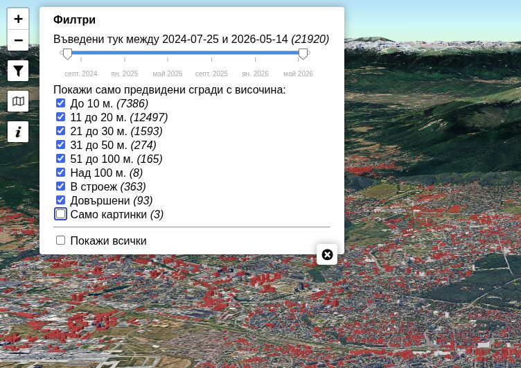
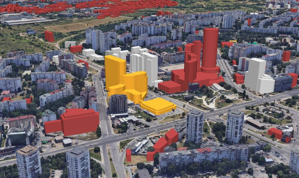
С тази цел добавих нова категория в 3D картата – проекти въведени само по картинки. За тези липсват скици, искания за ПУП или какъвто и да е процес в Столична община или СОС. По редица причини обаче имам достатъчно основания да смятам, че ще се случва в тези или аналогични параметри. Тук ще дам три примера и описвам защо съм ги добавил. По подразбиране са скрити на картата, но може да се покажат като отворите филтрите горе вляво и изберете категория „Само картинки“. Оцветил съм ги в златен цвят като компенсация за архитектите, които все негодуват колко грозни съм направил „следващите им зелени бижута“.
Залез над Дубайбад
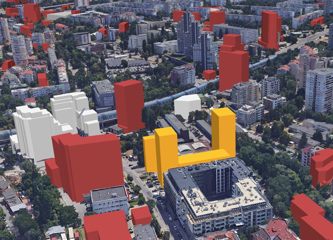
В квартал Дианабад, район Изгрев където метрото пресича ул. Тинтява се е сгушил огромен комплекс, който почти две години стоеше изоставен. Все още е на акт 14 и наскоро беше ребрандиран в опит все пак да продадат апартаментите в него. Обещанието на небезизвестният инвеститор Грийн Лайф е да бъде завършен през 2027-ма, когато се надяваме да разчисти и незаконното сметище за строителни отпадъци на територията на бъдещия линеен парк.
Срещу тази сграда вече има разрешение за строеж на друг 50 метрова. Нейният инвеститор предлага да облагороди подмостовото пространство, за да е по-малко шумно на бъдещите купувачи, а и вероятно да пасва по-добре визуални с двора на сградата му. Следващата сграда, която сега се завършва, е сравнително малка, но първо е върху земя отредена за обществено обсъждане, второ се намира направо върху колектор, в който е натикана река Новачица. Последното създаде проблеми с наводняване на гаражите по време на строежа, но съдът вече беше отредил, че проблем не вижда. По-надолу на мястото на сегашната бензиностанция Петрол се обсъжда няколко пъти в комисия изграждането на 75 метрова сграда. Именно от тези обсъждания стана ясно интересното становище от транспортен анализ, че улиците там са били толкова блокирани от трафик, че още 100 семейства в повече няма какво толкова повече да влошат положението. Проблемът е, че не са само 100 и не е само тази една или три сгради.
От документите на портала на общината разбираме, че по Тинтява на мястото на сегашния автосервиз залепена до сградата на АППК ще има друга 50 метрова сграда. Зоната е сМФ също както всички съседни. Странното определяне точно на тези имоти, както и следващия, за който ще говорим, буди съмнения за добре известния лобизъм в оформянето на ОУП на София. Тази сграда ще бъде съвсем близо до прозорците на ребрандираната Тинтява 80.
Наскоро ми изпратиха проект на още една 50 метрова сграда, която ще е отсреща на улицата. Инвеститорът Виа Ахинора е същият, който построи съседната сграда съдържаща клиника и ресторант Адела, но с практическа липса на озеленяване. Виждате я отбелязана в жълт… златно. За сградата няма искане за ПУП, виза или какъвто и да е публичен документ. Вече я рекламират на сайта си обаче и предвид зонирането и собствеността нямам съмнения, че ще я изпълнят както са решили. Картинките, разбира се, нямат общо с реалната ситуация в района, околните сгради зеленината и дори какво има в далечината. Друг проблем в случая е, че сградата ще е буквално на брега на река Новачица, която редовно прелива.
Това надали е известно на хората инвестирали вече в Тинтява 80, както и на онези замислящи се да купят от останалите апартаменти или в съседните изброени кули. Отделно, дори да се абстрахираме от плачевното състояние на улица Тинтява, тя е само 10 метра широка и практически без тротоари. Всичките ѝ изходи свършват в тапи, които и сега са крайно натоварени.
Единственото успокоение, ако може да се нарече така, е че съседният имот помещаващ сега Софтуни е собственост на Областна управа София. Т.е. държавна собственост. Той попада също в сМФ зона та ако правителството реши, може тихомълком да го продаде по отпаднала необходимост и да видим още една кула там и 30 хиляди кв.м. разгърната площ.
Към този „ансамбъл“, разбира се, следва да се добавят сградите на Артекс в близост, точно заради които в медиите се обсъжда, че са въведени лобистките промени в ЗУТ направили възможно всичко тук. В другата посока до метростанция Г.М. Димитров вече имаме данни за планираните кули на мястото на сградата на ПИБ.
Културна безстопанственост и фонд с история
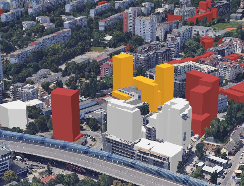
На метри от злополучното кръстовище на Тинтява ще има друг проект, за който се говори отдавна. Историята около Аудиовидео Орфей в квартал Изгрев е дълга и емблематична за липсата на интерес на Министерството на културата да опазва не само на културата, но държавната собственост. Препоръчвам статията на Mediapool, в която Радослав Александров проследява делата и участниците. Също текста на Генка Шикерова в Свободна Европа от 2023 г. Холдингът стоящ зад тази драма е свързван от самото начало с Иван Костов и Стефан Софиянски.
Тук нямаме картинка, на която да стъпим. От изхода на делото обаче знаем, че се предвижда строеж на ново студио за Орфей като компенсация. Знаем също, че зоната позволява до 75 метра височина и абсурднен кинт 3.5, т.е. могат да построят 92 хиляди кв.м. разгърната площ. Разбира се, има доста други изисквания като отстояние, озеленяване и прочие, които ще повлияят на крайния проект. Ако се опитаме да си представим възможното, за да се увеличи максимално печалбата от това парче земя, ще получим нещо подобно на снимката долу.
Нямаме представа дали в крайна сметка ще изглежда така. Тук виждаме само една възможност Теоретично може да решат да запазят стила на квартала, да се концентрират върху качество, спокойствие, разумно строителство и реална зеленина, а не 5-те см. почва на Артекс. Това би било прекрасно, но предвид всичко видяно в града по-скоро се съмнявам. На този етап няма никаква публична информация или задействан процес. Ще обновя картата когато научим нещо.
Детска градина – залагалка
Говорейки за Артекс третият проект е техен. Отдавна се говори, че ще се строи нещо на мястото на Била в квартал Младост. Научихме какво миналата година от серия интервюта на собствениците на строителната фирма. Еднотипното съдържание, което само на места беше отбелязано като платено, каквото е изискването, видимо целеше да промотира проекта като едва ли не „полезен“ за квартала. Описват как ще подаряват детска градина на града. Аз го описах като подигравка и зададох насрещни въпроси като това кой ще поема разходите за довършителните работи, дали ще плащат родителите вход, за да влизат в комплекса. Най-вече дали наистина общината ще притежава имот или само акции в дружество, което реално държи сградата по добре познатата и опасна схема за избягване на данъци, в която НАП ги обвини. Що се отнася до публична инфраструктура и дарения на общината обаче, бих бил много внимателен какво всъщност правят и какво качество доставя Артекс предвид видимите резултати наскоро.
Картинката им от октомври 2025
Картинката от януари 2026
През януари виждам, че отново са говорили за сградата и са пуснали нови визуализации. В тези, както и предишните се забелязва, че са използвали аналогични полигони на тези в 3D картата ми, но сиви. Всъщност, не са аналогични – използвали са буквално стара версия на данните ми във визуализацията си. Точно това е целта на картата и се радвам, че е била полезна на тях или хората, които са наели да им правят картинките. При това условие обаче нямат право да я критикуват като неточна. Дори би следвало да се радват, че по снимките включвам модел на сградата им тук.
Този проект също няма задействана процедура, обсъждания или някаква публична информация извън опитите на Мирянови да омилостивят общественото внимание. Включвам я първо заради историята на Артекс в „магическо“ преодоляване на всякакви административни, законодателни и съдебни пречки. Второ, защото нямам съмнение, че след отшумяването на скандала с другия проект за 75 метрова сграда, районният кмет на Младост Кукурин ще лобира от името и на този инвеститор пред общината, СОС и жителите на квартала.
В съседство виждате вече строяща се друга сграда-стена пак на Артекс. Зад нея е старият неосъществен проект на Гаранти Коза. За него съм сигурен, че няма да изглежда така в бъдеще, но нямаме данни за промяна. Затова, както с другите над 20 хиляди сгради в София, разчитам на наличните документи.
Много шум за нещо
Изключение от това правило са тези три сгради и има причини да бъдат включени. Целта е същата както с целия проект – да информира за потенциалното строителство в София, как е замислено и какво е възможно. Почти всички сгради, които виждате, са одобрени от години или най-малкото строеж на това място с конкретните параметри е подсигурено административно с решения на СОС и/или ПУП-ове отдавна. Оперативно общината в момента може да забави или изиска корекция, но рядко да спре строеж. Без промени в ОУП, ЗУТ и Закона за София от страна на парламента, без строго съблюдаване на изпълнението на параметрите и озеленяването от ДНСК и самата община, но дори по-важно – без постоянство в съдебната практика и поне някакво разумно намаление на корупцията в административните съдилища, почти сигурно всичко червено на картата ще стане сиво от бетон. Разбира се, действията и практиките в общината са важни, но са предимно следствие и се движат в рамките на описаното.
Осъзнавам, че картата създава шум, който дразни инвеститори и създава допълнителна работа на общината. Всъщност, бивш и.д. главен архитект на София не пропусна да ме нахока точно за това в началото на миналата година настоявайки освен всичко друго, че изискванията за озеленяване са глупост и няма такова нещо като презастрояване. Отчитам, че картата понякога не се разбира въпреки подробно описаната методология. В същото време е вярно, че служи като инструмент за визуализация на притеснителни ситуации из града, които все по-често виждаме да се материализират. В този мисъл още тогава отговорих, че проблемът не е моето представяне, а в липсата на проследимост и абсолютна прозрачност от край до край на процеса, разбиране у обществото на базовите проблеми в градоустройството в София и да – липсата на доверие.
В посока на една от тези точки би помогнал отдавна закъснелият регистър по начина, по който е предложен от служебния министър Николай Найденов и съдържащ дигитално досие на всички такива планове и строежи в цялата страна. Както и другите отворени от него данни, този регистър ще предложи степен на прозрачност и свързаност на информацията надминаващо дори напредъка на София в последните две години. Сега постановлението е на етап съгласуване. Ако настоящото правителство на Радев реши да не спъне и тази прозрачност, каквито съмнения има, че се случва с данните на МВР и МРРБ, ще видим 3D карта като моята, но за цяла България.
Ако попаднете на други подобни реклами на сгради, за които не намирате информация, ще се радвам да ми ги изпратите. Ще се разровя и преценя дали може да се поместят на картата.
Amazon S3 Tables with Amazon Redshift gives you a powerful combination for analytical workloads on Apache Iceberg tables. But as query volumes grow, small inefficiencies compound. For example, repeated queries, such as dashboards refreshing hourly or analysts running the same joins throughout the day, scan data directly from Amazon Simple Storage Service (Amazon S3) every time. The fully qualified three-part table references ([email protected]) add friction for business intelligence (BI) tools and end users who expect simpler SQL syntax. And without tuning the way S3 Tables organizes your data files, queries read more files than necessary. When you address these three areas, your S3 Tables queries in Amazon Redshift become faster, simpler, and more cost-efficient, whether you’re powering a recurring dashboard or supporting ad hoc analysis at scale.
This is the third post in our S3 Tables and Amazon Redshift series. The first post covered getting started with querying Apache Iceberg tables, and the second post walked through enterprise-scale governance and access controls. In this post, you address those performance and usability gaps with three approaches:
Create external schemas to simplify queries from three-part notation down to two-part notation.
Build materialized views that store pre-computed results locally so repeated queries skip the S3 scan.
Configure S3 Tables compaction strategies so the data file layout matches your query patterns.
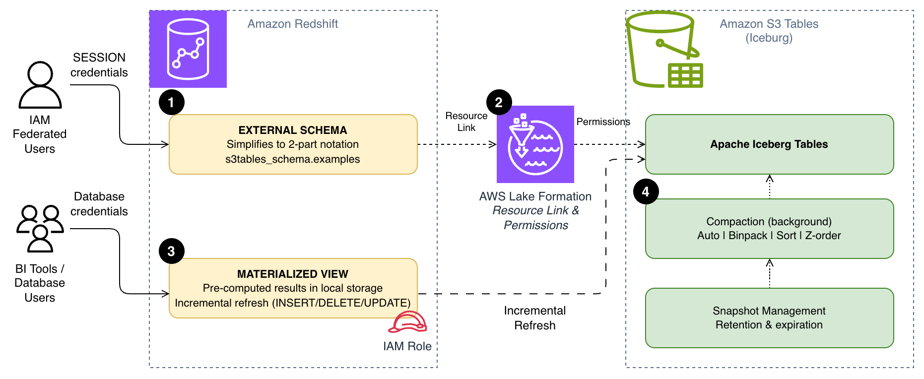
The following diagram shows how these three approaches work together. External schemas [1] simplify query syntax through AWS Lake Formation resource links [2], materialized views [3] store pre-computed results locally in Amazon Redshift, and S3 Tables compaction [4] optimizes the underlying file layout for your query patterns.
You can use this syntax, but it can be cumbersome in business intelligence (BI) tools, manually typing queries, and in application code. This syntax also requires the user to use IAM federation. By creating an external schema, you can reference the same tables with a concise two-part notation:
SELECT * FROM s3tables_schema.examples;
To set this up, you create a Lake Formation resource link that maps to your S3 Tables catalog, then create an external schema in Amazon Redshift that points to that resource link. Your setup differs slightly depending on whether your users authenticate through IAM federation or database credentials. While this doesn’t change query performance, it removes a common barrier to adoption by simplifying the reference.
Create a Lake Formation resource link
Both authentication methods require a resource link in Lake Formation that points to your S3 Tables database.
In the Lake Formation console, choose Databases under Data Catalog.
On the Create menu, choose Resource link.
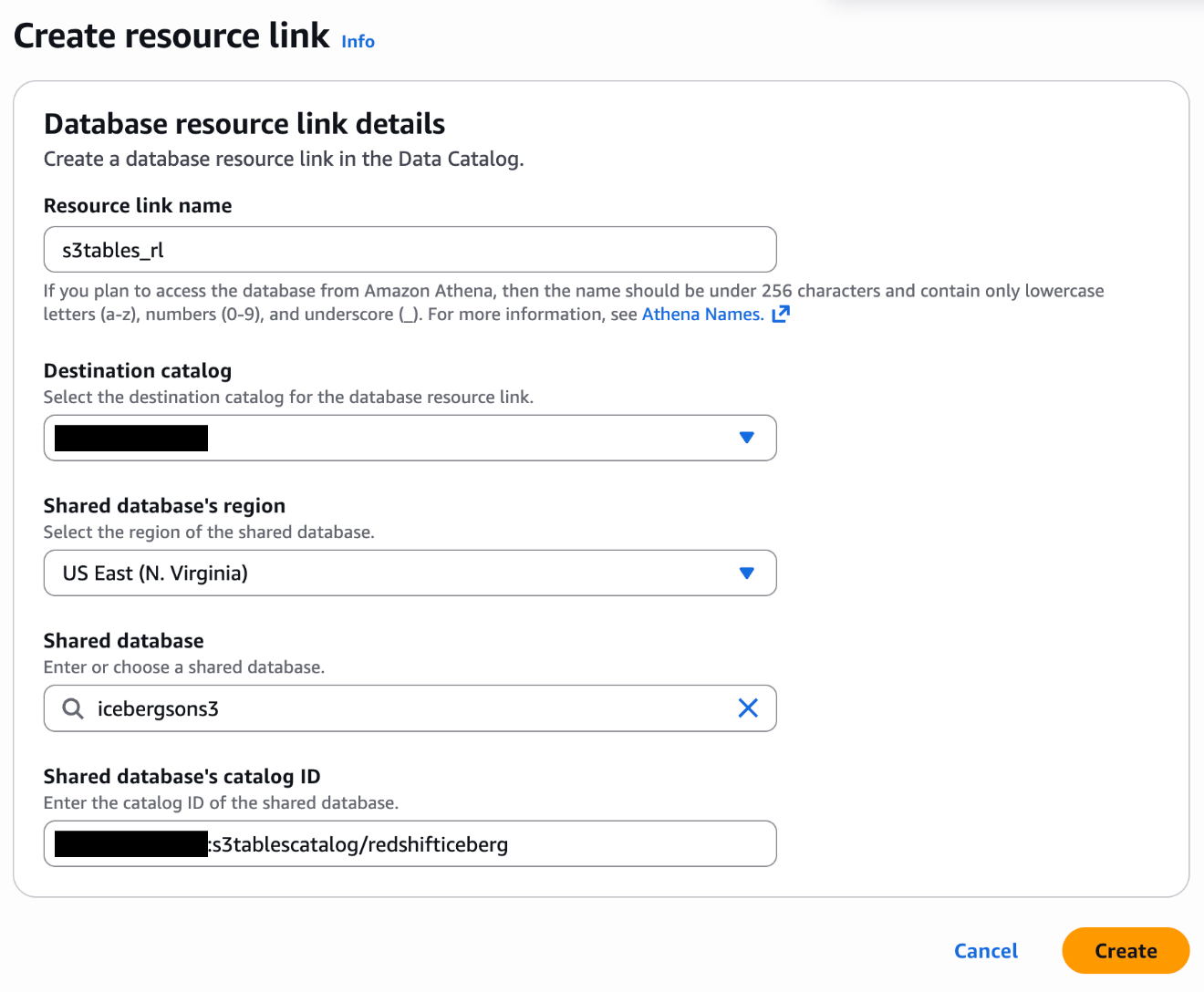
Configure the resource link with the following settings:
Resource link name:s3tables_rl
Destination Catalog: Your account ID (for example, 111122223333)
Shared Database: Your S3 Tables database (for example, icebergsons3)
Shared Database’s Catalog ID: Your S3 Table bucket in the format 111122223333:s3tablescatalog/redshifticeberg
If your users connect to Amazon Redshift through IAM federation, create the external schema with the SESSION keyword. This passes the federated user’s credentials through to Lake Formation for access control:
CREATE EXTERNAL SCHEMA s3tables_schema
FROM DATA CATALOG
DATABASE 's3tables_rl'
CATALOG_ID '111122223333'
IAM_ROLE 'SESSION'
CATALOG_ROLE 'SESSION';
Lake Formation evaluates your permissions based on your federated user’s IAM role, and sees only the tables and columns their role allows. This is the recommended approach for new deployments because it provides fine-grained access control without additional role management.
Option B: External schema for database users
External applications like Tableau, PowerBI, and custom ETL tools often authenticate with database credentials instead of IAM federation. These users need an IAM role to access S3 Tables on their behalf.
Create an IAM service role to access S3 Tables:
You create a role (for example, S3TableAccessRole) with a trust policy that allows Amazon Redshift to assume it:
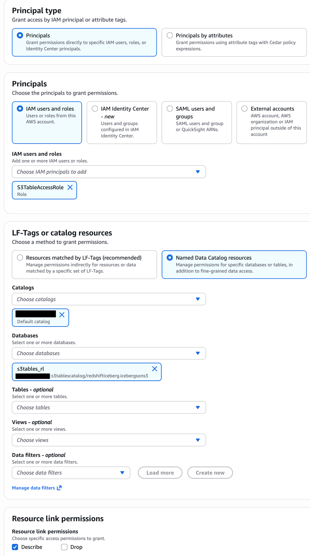
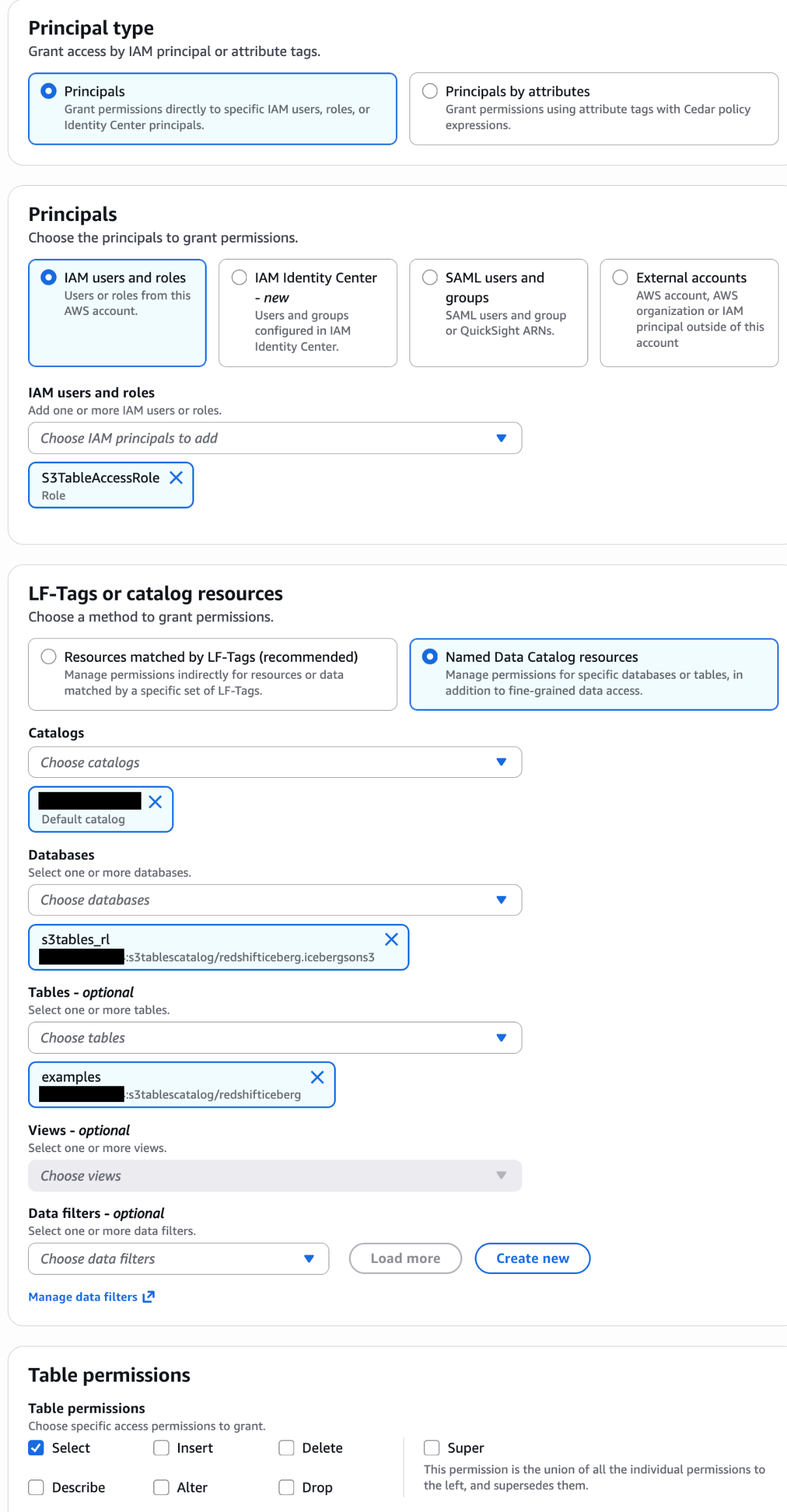
In the Lake Formation console, grant the S3TableAccessRole DESCRIBE access on the database and SELECT access on the tables for your resource link. For detailed steps, see Granting Lake Formation permissions.
CREATE EXTERNAL SCHEMA s3tables_schema
FROM DATA CATALOG
DATABASE 's3tables_rl'
IAM_ROLE 'arn:aws:iam::111122223333:role/S3TableAccessRole';
Then grant access to your database users:
GRANT USAGE ON SCHEMA s3tables_schema TO my_database_user;
Query with two-part notation
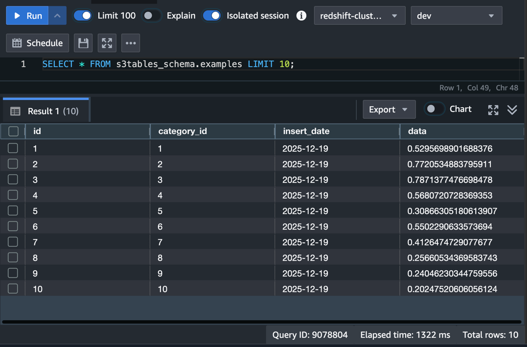
With either option, you can now query S3 Tables using the simpler two-part notation:
SELECT * FROM s3tables_schema.examples LIMIT 10;
You can use this notation in BI tools, JDBC/ODBC connections, and application code and no longer need to know the underlying catalog structure.
Accelerate queries with materialized views
When you repeatedly query S3 Tables, each execution scans the external data from S3. Materialized views store pre-computed results in Amazon Redshift, so subsequent queries read from local storage instead of scanning S3 on every run.
Redshift supports incremental refresh for materialized views on Apache Iceberg tables, including INSERT, DELETE, UPDATE, and table compaction operations. After the initial creation, Amazon Redshift processes only the rows that changed since the last refresh when you run subsequent refreshes, rather than recomputing the full result set. This helps reduce both the time and compute cost of keeping your views current, especially for large tables with frequent changes.
The following example creates a materialized view that joins the examples table in S3 Tables with a local categories table in Amazon Redshift. You can use a materialized view to pre-compute daily record counts and data samples per category:
CREATE MATERIALIZED VIEW mv_daily_category_summary
DISTSTYLE KEY
DISTKEY (category_id)
SORTKEY (insert_date)
AS
SELECT
    c.category_id,
    c.department,
    e.insert_date,
    COUNT(*) AS record_count,
    COUNT(DISTINCT e.id) AS unique_ids
FROM s3tables_schema.examples e
JOIN public.categories c
  ON c.category_id = e.category_id
GROUP BY c.category_id, c.department, e.insert_date;
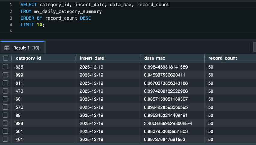
Query the materialized view directly:
SELECT category_id, department, insert_date, record_count
FROM mv_daily_category_summary
ORDER BY record_count DESC
LIMIT 10;
Your query can now read from local Amazon Redshift storage and typically returns results without scanning S3 Tables:
Refresh strategies
You have two options for keeping materialized views current:
Automatic refresh: Set AUTO REFRESH YES in the view definition to have Amazon Redshift automatically refresh the view in the background when it detects changes to the base tables. This is a good fit for dashboards and reports that can tolerate a short delay between data changes and query results. Note that automatic refresh requires Option B (database user) when creating the external schema, and the default is AUTO REFRESH NO.
Manual refresh: Run REFRESH MATERIALIZED VIEW when you need to control the timing:
Use manual refresh when you need to coordinate updates with data loading pipelines or when you want to refresh during off-peak hours.
Tune S3 Tables compaction for your query patterns
S3 Tables automatically compacts small Parquet files into larger ones in the background. This compaction reduces the number of read requests your query engine must make, which can improve query performance. By default, compaction targets a file size of 512 MB, configurable between 64 MB and 512 MB. Four compaction strategies are available, and choosing the right one for your query patterns can make a measurable difference.
Compaction strategies
Strategy
When to use
How it works
Auto
You want S3 to decide for you
Selects sort compaction for sorted tables, binpack for unsorted tables
Binpack
General-purpose workloads, unsorted tables
Combines small files into larger files (100 MB+) and applies pending row-level deletes
Sort
Queries frequently filter on a single column (e.g., insert_date)
Organizes data by the table’s sort-order columns during compaction
Z-order
Queries filter on two or more columns together (e.g., insert_date and category_id)
Blends multiple column values into a single scalar for sorting
Binpack improves performance by reducing the number of files a query engine reads. Sort compaction goes further. By ordering data within files, it enables query engines to skip entire files based on column min/max metadata during predicate pushdown. This is effective for queries that filter on the sort column, such as date-range filters. Z-order extends this benefit to queries that filter on multiple columns simultaneously, at the cost of slightly less efficient pruning on any single column compared to a pure sort.
To use sort or z-order compaction, you first need to verify that the table is sorted by one (sort) or multiple (z-order) columns:
-- Sort
ALTER TABLE icebergsons3.examples WRITE ORDERED BY insert_date;

-- Z-Order
ALTER TABLE icebergsons3.examples WRITE ORDERED BY insert_date,category_id;
S3 Tables manage snapshots automatically. By default, it keeps a minimum of 1 snapshot and expires snapshots older than 120 hours (5 days). The snapshot retention is customized by setting minSnapshotsToKeep and maxSnapshotAgeHours. After a snapshot reaches the expiration time you configured in your retention settings, S3 Tables marks objects that only that snapshot references as noncurrent and removes them based on the unreferenced file removal policy.
You can adjust these settings if your workload needs more snapshots for time-travel queries or longer retention:
Keep in mind that retaining more snapshots increases storage costs. If a materialized view references an expired snapshot, Amazon Redshift falls back to a full recompute on the next refresh. Therefore, snapshot retention can directly affect your materialized view refresh behavior. Balance snapshot retention with your materialized view refresh frequency to avoid unnecessary full recomputes.
Choose the right access pattern for your users. Use IAM federation with SESSION credentials for new applications and interactive users. Reserve the IAM role approach for BI tools and extract, transform, and load (ETL) pipelines that can’t integrate with IAM federation directly. Plan to migrate database users to federated access over time.
Match compaction strategy to query patterns. Use sort compaction when your queries filter on a single column (such as date ranges). Use z-order when queries filter on two or more columns together. Stick with the auto default if your query patterns vary or you’re unsure.
Size materialized views for your refresh window. Materialized views that join large external tables with local tables take longer to refresh. If your data changes frequently, keep the materialized view focused on the specific aggregations your dashboards need rather than materializing entire tables.
Coordinate snapshot retention with materialized view refresh. If a materialized view references an expired Iceberg snapshot, Amazon Redshift performs a full recompute instead of an incremental refresh. Set your snapshot retention (maxSnapshotAgeHours) longer than your materialized view refresh interval.
Monitor compaction with AWS CloudTrail. S3 Tables logs compaction operations as CloudTrail management events. Track these to verify that compaction runs on schedule and to identify tables that might benefit from a different strategy.
Balance performance gains against storage costs. Materialized views store pre-computed results in Amazon Redshift, adding to your managed storage. Compaction reduces file counts, but z-order and sort compaction can increase overall storage because of data duplication across sort boundaries. Review your Amazon Redshift managed storage usage and S3 Tables storage metrics periodically to make sure the performance benefits justify the additional storage utilization.
Troubleshooting
Issue
Resolution
“Permission denied” when creating the external schema
Verify the IAM role has lakeformation:GetDataAccess permission. Confirm you associated the role with your Amazon Redshift cluster or workgroup. Also check that you granted the role access to the resource link database and its tables in Lake Formation.
“Schema not found” or “Database not found” errors
Confirm the resource link name in Lake Formation matches the DATABASE value in your CREATE EXTERNAL SCHEMA statement. Verify the catalog ID format uses the pattern account_id:s3tablescatalog/bucket_name.
“Table not found” when querying through the external schema
Check that Lake Formation permissions include table-level access, not just database-level. Verify the table exists in the S3 Tables catalog by querying it through the auto-mounted catalog first.
Materialized view refresh falls back to full recompute
Check if the referenced Iceberg snapshot has expired. Increase maxSnapshotAgeHours in the snapshot management configuration. Verify that the base table hasn’t exceeded 4 million position deletes in a single data file. Compaction resolves this.
Queries on S3 Tables are slow after data loading
Compaction runs on an automated schedule and may not have processed recent writes yet. Check CloudTrail for the latest compaction event. Verify the compaction strategy matches your query patterns. Switch from binpack to sort if you filter on specific columns.
Cleaning up
To avoid ongoing costs, remove the resources you created in this walkthrough:
-- Drop materialized views
DROP MATERIALIZED VIEW IF EXISTS mv_daily_category_summary;

-- Drop external schemas
DROP SCHEMA IF EXISTS s3tables_schema;
Also remove:
The IAM role (S3TableAccessRole) and its attached policies, if you created one for database users.
The Lake Formation resource link and associated permissions.
In this post, we showed how to optimize S3 Tables queries from Amazon Redshift using three approaches: external schemas that simplify query syntax from three-part to two-part notation, making it easier for BI tools and end users to work with S3 Tables. We also covered materialized views for pre-computed analytical results that reduce repeated S3 scans, and S3 Tables compaction strategies tuned to your query patterns for more efficient file access.
For new applications, design your access layer with IAM federation and external schemas from the start. Use materialized views to accelerate repeated analytical queries that join S3 Tables with local Amazon Redshift data. Match your compaction strategy to how your team queries the data. Use sort compaction for date-range filters and z-order when queries filter on multiple columns at once. Furthermore, the same S3 tables you optimize here are also accessible from Amazon Athena, Amazon EMR, and third-party engines.
Migrating your TLS endpoints to Post-quantum cryptography (PQC) starts with understanding your current TLS endpoint inventory and posture. This post introduces the PQC Readiness Scanner — an automated tool that inventories your Application Load Balancer (ALB), Network Load Balancer (NLB), and Amazon API Gateway endpoints and continuously monitors their TLS configurations for PQC readiness. The scanner classifies each endpoint into a three-tier framework that helps prioritize and plan PQC migration.
As quantum computing advances, you need to migrate to quantum-resistant cryptography to protect your data long-term. The PQC Readiness Scanner helps you identify which endpoints to migrate first and tracks your progress across accounts. For web traffic, PQC key exchange algorithms are negotiated only within TLS 1.3. This means quantum-resistant connections require endpoints that support TLS 1.3 and PQC key exchange.
Under the AWS Shared Responsibility Model, AWS secures the infrastructure and enables PQC support across its services. Customers are responsible for configuring their resources to use PQC-capable TLS policies. For AWS-terminated TLS connections—such as those on Application Load Balancer (ALB),Network Load Balancer (NLB), Amazon API Gateway, and Amazon CloudFront—customers choose the security policy (an AWS-managed configuration defining supported TLS protocol versions and cipher suites for a listener) that determines TLS version and cipher suite, key exchange, and authentication algorithm support.
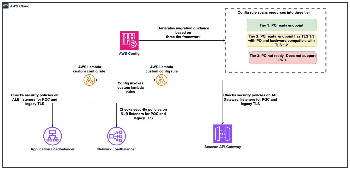
The automated PQC Readiness Scanner for AWS-terminated TLS endpoints is built using AWS Config conformance packs. A conformance pack is a collection of AWS Config rules and remediation actions that can be deployed as a single entity in an account and a Region or across an organization in AWS Organizations.
Solution overview
The PQC Readiness Scanner deploys AWS Config rules using a conformance pack to evaluate the security policy on each endpoint. Based on the evaluation, each resource is classified into a three-tier readiness framework that prioritizes migration actions needed to achieve PQ-ready TLS.
The PQC Readiness Scanner performs two checks per resource:
Does the endpoint use a PQ-ready security policy?
Does the endpoint support legacy TLS 1.0 or 1.1?
Each check returns COMPLIANT or NON_COMPLIANT status with specific policy recommendations.
PQC requires endpoints to support TLS 1.3 and use PQC key exchange algorithms. The three-tier framework helps you interpret findings and prioritize fixes. The goal is to have TLS 1.3 with PQC key exchange enabled on the endpoints. However, achieving this requires maintaining backward compatibility with clients.
Tier
Readiness level
TLS protocols
PQC status
Migration priority
Tier 1
PQ-ready (strongest posture)
TLS 1.3 only with PQC key exchange
PQ-ready
None
Tier 2
PQ-ready (backward compatible)
TLS 1.2 and 1.3 with PQC key exchange
PQ-ready
Low
Tier 3
Not PQ-ready
No PQC key exchange
Not PQ-ready
High
How to prioritize your migrations
Tier 1 represents the strongest security using only TLS 1.3 with PQC key exchange. These resources already meet the target state.
Tier 2 represents a backward-compatible PQ-ready configuration. Endpoints support both TLS 1.2 and TLS 1.3, with PQC key exchange negotiated on TLS 1.3 connections. Migration priority is low because these resources already provide quantum-resistant protection for clients that support TLS 1.3, while maintaining TLS 1.2 compatibility for legacy clients. Migrate to Tier 1 when client-side analysis confirms that the connecting clients support TLS 1.3 with PQC key exchange.
Tier 3 covers resources that aren’t PQ-ready. This includes endpoints without TLS 1.3 support, endpoints with TLS 1.3 but without PQC key exchange policies. These resources require immediate attention.
Assessment scope
The scanner evaluates the following AWS edge services that terminate TLS connections on behalf of your applications.
Edge services:
Application Load Balancer (ALB), Network Load Balancer (NLB) listeners with HTTPS, TLS, and TCP SSL protocols are evaluated.
API Gateway REST APIs are evaluated for AWS Regional and private endpoints along with API Gateway HTTP APIs (v2) and WebSocket APIs (v2).
Excluded edge services:
CloudFront distributions are excluded from the PQC readiness scope because TLS 1.3 with hybrid post-quantum key exchange is automatically enabled across existing CloudFront TLS security policies for viewer-to-edge connections. No customer action is required for inbound (viewer-facing) PQC on CloudFront.
Recommended approach for Classic load balancer:
For Classic Load Balancers, AWS recommends migrating to ALB or NLB. Classic Load Balancers don’t support TLS 1.3 or PQC key exchange and can’t be made PQ-ready.
How the solution works
AWS Config enables continuous monitoring and evaluation. Conformance packs enable organization-wide deployment. AWS Lambda is a serverless compute service that runs code to perform security policy evaluation based on the AWS Config rules. AWS Serverless Application Model (AWS SAM) is an open source framework used for deploying the AWS Lambda functions.
Figure 1: PQC readiness solution architecture
The PQC Readiness Scanner conformance pack implements four custom AWS Config rules powered by two Lambda functions:
Rule
What it checks
Non-compliant result
ELB PQ-ready
Load balancer listeners use security policies that support TLS 1.3 with PQC key exchange algorithms
Policy doesn’t include PQC support, the resource is marked with a recommended upgrade policy
ELB legacy TLS
Load balancer listeners allow TLS 1.0 or 1.1 connections
Legacy protocols are configured, the resource is flagged.
API Gateway PQ-ready
API Gateway endpoints use security policies that support TLS 1.3 with PQC key exchange algorithms
Policy doesn’t include PQC support, the resource is marked with a recommended upgrade policy
API Gateway legacy TLS
API Gateway endpoints allow TLS 1.0 or 1.1
Legacy protocols are configured, the resource is flagged.
Deploy the PQC Readiness Config Scanner in three phases. Complete deployment commands and configuration details are available in the GitHub repository. The Lambda functions must be deployed first because the conformance pack references their ARNs as parameters. See the GitHub repository for details.
Deploy to single account:
Clone and Build:
git clone https://github.com/aws-samples/sample-PQC-Readiness-using-AWS-Config.git

cd sample-PQC-Readiness-using-AWS-Config/installation

sam build
Deploy to One or More Regions:
# Make script executable (first time only)
chmod +x deploy-per-regions.sh

# Deploy to a single region
./deploy-per-regions.sh us-east-1

# Deploy to multiple regions
./deploy-per-regions.sh us-east-1 us-west-2 eu-west-1
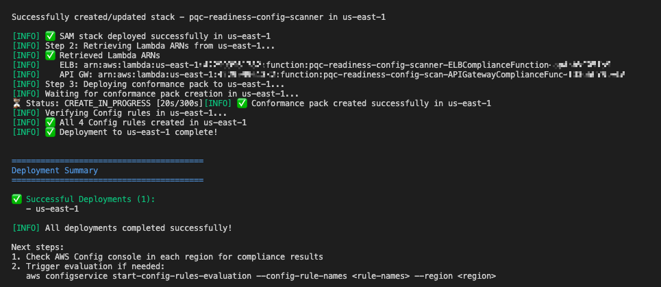
Figure 2: Type y and continue if you have enabled AWS Config recording for these resources or its by default recording all resources.
The script automatically:
Deploys Lambda functions via SAM
Deploys conformance pack (creates Config rules)
Verifies deployment success
Provides clear status messages
The deployment creates two Lambda functions that perform PQ-ready and legacy TLS checks. It provisions IAM roles with least-privilege permissions for ELB, ALB, NLB, and API Gateway describe operations. Lambda permissions allow AWS Config to invoke the functions.
Figure 3: Example screen-print of what a successful deployment looks like.
Multi-account deployment (Organizations):
For organization-wide deployment across multiple AWS accounts, use CloudFormation StackSets to deploy Lambda functions to each account.
Important Constraint: AWS Config CUSTOM_LAMBDA rules require the Lambda function to exist in the same account as the Config rule. You cannot use a centralized Lambda in one account to evaluate resources in other accounts.
Prerequisite: Shared S3 Bucket
Before packaging, create an S3 bucket accessible by each target account in your organization. This bucket will host the Lambda deployment artifacts that CloudFormation StackSets pulls into each member account.
# Create the shared S3 bucket (run from management/central account)
aws s3 mb s3://<your-org-shared-bucket> --region us-east-1
Grant read access to the target accounts using one of the following options:
Replace <account IDs> with the AWS account IDs where StackSets will deploy the Lambda functions.
Note: The bucket must be in the same region as the StackSet deployment regions. For multi-region deployments, create one bucket per region and run sam package separately for each.
Step 1: Build and Upload Lambda Packages to S3
Run the packaging script from the installation/ directory:
cd installation

# Make script executable (first time only)
chmod +x deploy-stacksets.sh

# Build, package, upload to S3, and generate resolved template
./deploy-stacksets.sh <your-org-shared-bucket>
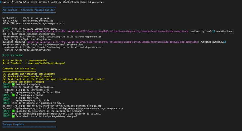
This script automatically:
Builds Lambda functions using SAM
Creates ZIP packages
Uploads ZIPs to the shared S3 bucket
Generates packaged-template.yaml with S3 values baked in (no parameters needed at deploy time)
Figure 4: Sample script output of successful upload of the lambda packages to S3 bucket
Step 2: Deploy Lambda Functions via StackSets
Run the following from the management account (or delegated admin account):
# Create StackSet (--region sets the StackSet "home region" where it is managed)
aws cloudformation create-stack-set \
  --stack-set-name pqc-readiness-lambda-functions \
  --template-body file://packaged-template.yaml \
  --capabilities CAPABILITY_IAM \
  --permission-model SERVICE_MANAGED \
  --auto-deployment Enabled=true,RetainStacksOnAccountRemoval=false \
  --region us-east-1

# Deploy stack instances to member accounts
# --regions = target regions where Lambda functions are deployed in member accounts
# --region  = must match the StackSet home region above
aws cloudformation create-stack-instances \
  --stack-set-name pqc-readiness-lambda-functions \
  --deployment-targets OrganizationalUnitIds=ou-xxxx-xxxxxxxx \
  --regions us-east-1 \
  --region us-east-1
Important — StackSet home region vs deployment regions:
--region (on each CLI command) = the StackSet home region where the StackSet resource lives. Subsequent operations (describe, update, delete) must specify this same region.
--regions (on create-stack-instances) = the deployment target region(s) where stack instances are created in member accounts.
These are independent values. Specify --region explicitly to avoid accidental deployment to your CLI’s default region.
Note: SERVICE_MANAGED StackSets must be created from the management or delegated admin account. The management account itself is excluded from stack instance deployments — use deploy-per-regions.sh separately if you need the scanner in the management account.
This creates Config rules in each member account that reference their local Lambda functions.
Migration guidance and prioritization
The three-tier system provides PQC migration priorities:
High priority – Tier 3 (not PQ-ready):
Target: Resources without PQC support. This includes endpoints not using PQ-ready security policies, endpoints that still allow TLS 1.0 or 1.1.
Action: Upgrade to a PQ-ready policy containing PQ in its name, such as those ending with -PQ-2025-09 (see Elastic Load Balancing security policies documentation for the full list).
Important: Before upgrading to a PQ-ready policy, audit your client TLS versions. PQ-ready policies require TLS 1.3 support; legacy clients that only support TLS 1.2 or earlier will fail to negotiate a connection. Start with a Tier 2 backward-compatible policy (which supports both TLS 1.2 and 1.3 with PQC), monitor connection logs for TLS negotiation failures, and only move to a Tier 1 TLS 1.3-only policy after confirming that your clients support TLS 1.3 with PQC key exchange.
Risk: Endpoints don’t support post-quantum cryptography for data in transit. Legacy TLS protocols are vulnerable to current cryptographic attacks.
Target: Resources using TLS 1.3 + PQ-ready policies that also support TLS 1.2 for backward compatibility.
Action: Consider TLS 1.3-only policies when client compatibility analysis confirms connecting clients support TLS 1.3.
Risk: Minimal. These resources already support PQ-TLS with TLS 1.3 connections. TLS 1.2 and earlier fallback maintains backward compatibility, which might indicate some clients aren’t negotiating in PQ-TLS. Remediation is to monitor logs, identify the volume of these connections and clients and plan migration for these clients to use TLS 1.3 with PQ-TLS.
No action – Tier 1 (PQ-ready, optimal):
Target: Resources using TLS 1.3 only with PQC key exchange: These resources meet the target state. No migration needed.
Viewing the results
In each member account, navigate to AWS Config Console in the deployed region.
Conformance Pack View
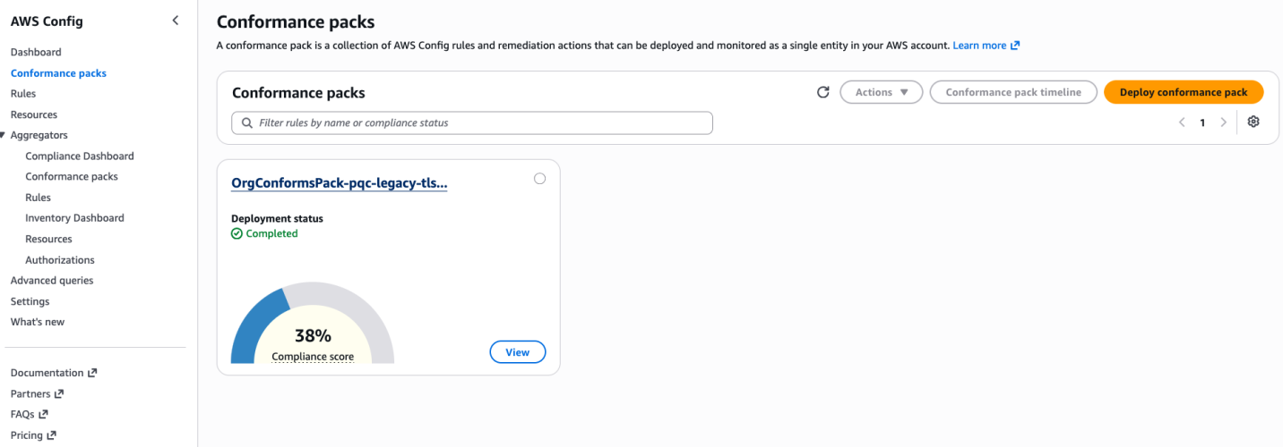
Go to AWS Config → Conformance packs and look for:
OrgConformsPack-pqc-legacy-tls-compliance-
Note: Organization conformance packs are prefixed with OrgConformsPack- and have a random suffix appended (e.g., OrgConformsPack-pqc-legacy-tls-compliance-gyv22je0).
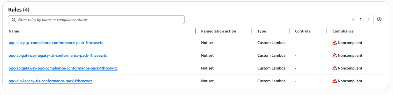
Figure 5: PQC Conformance Pack Compliance Score is the percentage of the number of compliant rule-resource
Click the conformance pack to see an overall compliance summary across all 4 rules.
Individual Rules View
Go to AWS Config → Rules and find 4 rules with prefix pqc-:
pqc-elb-pqc-compliance-conformance-pack-
pqc-elb-legacy-tls-conformance-pack-
pqc-apigateway-pqc-compliance-conformance-pack-
pqc-apigateway-legacy-tls-conformance-pack-
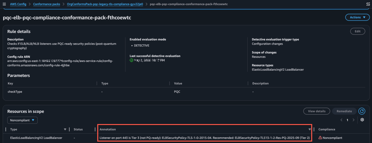
Click any rule to view:
Compliant vs non-compliant resource counts
Detailed annotations for each resource
Resource ARNs and current security policy configurations
Figure 6: Visibility into Config rules status inside the conformance pack
Figure 7: Sample image of the config rule findings and annotation describing the migration guidance based on 3-tier classification.
Conclusion
After deploying the PQC Readiness Scanner, you gain visibility into TLS posture across AWS edge services, which reduces manual configuration reviews. The tier system provides specific upgrade recommendations so teams can understand next steps without cryptographic expertise. The scanner automatically detects configuration changes to help new deployments maintain readiness standards. Built-in AWS Config reporting supports audit requirements and demonstrates measurable progress toward PQC readiness.
Deploy the PQC Readiness Scanner and review your results with PQC Readiness Scanner. Start migration with high priority Tier 3 resources and monitor progress across your accounts using AWS Config aggregators.
If you have feedback about this post, submit comments in the Comments section below. If you have questions about this post, start a new thread on AWS Config re:Post or contact AWS Support.
I’m speaking at the Potsdam Conference on National Cybersecurity at the Hasso Plattner Institut in Potsdam, Germany. The event runs June 24–25, 2026, and my talk will be the evening of June 24.
When you’re working through a backlog—opening an issue, jumping to a linked thread, then back to the list—latency isn’t just a metric. It’s a context switch. Even small delays add up, and they hit hardest at the exact moments developers are trying to stay in flow. It’s not that GitHub Issues was “slow” in isolation; it’s that too many navigations still paid the cost of redundant data fetching, breaking flow again and again.
Earlier this year, we set out to fix that—not by chasing marginal backend wins, but by changing how issue pages load end-to-end. Our approach was to shift work to the client and optimize perceived latency: render instantly from locally available data, then revalidate in the background. To make that work, we built a client-side caching layer backed by IndexedDB, added a preheating strategy to improve cache hit rates without spamming requests, and introduced a service worker so cached data remains usable even on hard navigations.
In this post, we’ll walk through how the system works and what changed in practice. We’ll cover the metric we optimized for; the caching and preheating architecture; how the service worker speeds up navigation paths that used to be slow; and the results across real-world usage. We’ll also dig into the tradeoffs—because this approach isn’t free—and what still needs to happen to make “fast” the default across every path into Issues. If you’re building a data-heavy web app, these patterns are directly transferable: you can apply the same model to reduce perceived latency in your own system without waiting for a full rewrite.
The speed of thought: Web performance in 2026
In 2026, “fast enough” is not a competitive bar. For developer tools, latency is product quality. When someone is triaging multiple issues, reviewing a feature request or reporting a bug, every avoidable wait breaks flow.
Modern local-first tools and aggressively optimized clients have moved the standard from “loads in a second” to “feels instant.” In this world, users do not benchmark us against old web apps. They benchmark us against the fastest experience they have ever had every day.
GitHub Issues is not a small surface area. Every week millions of people around the world rely on Issues to keep their codebase running smoothly. As Issues also becomes the planning layer for AI-assisted work, perceived performance becomes even more critical: if the loop between intent and feedback is slow, the entire system feels slow.
We heard the same problems from both internal teams and the community: Issues felt too heavy compared to tools built with speed as a first principle. The bottleneck was not feature depth or correctness. It was architecture and request lifecycle. Too many common paths still paid the full cost of server rendering, network fetches, and client boot, even when data had effectively been seen before.
Our Issues Performance team’s job was to close that gap. The objective was straightforward and technical: redesign data flow and navigation behavior so the product feels instant by default.
Before changing architecture, we needed to align on what “fast” means in user terms and how to measure it. Generic page metrics are useful, but they are not sufficient for a complex product surface like Issues.
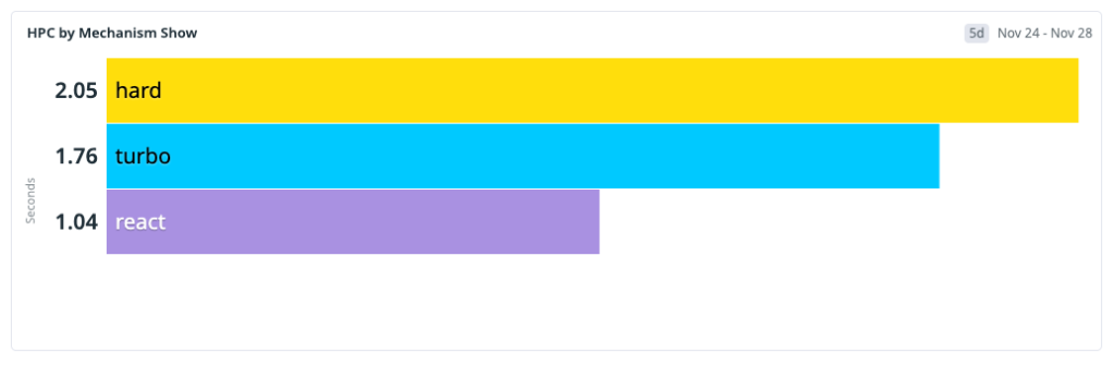
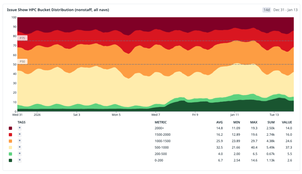
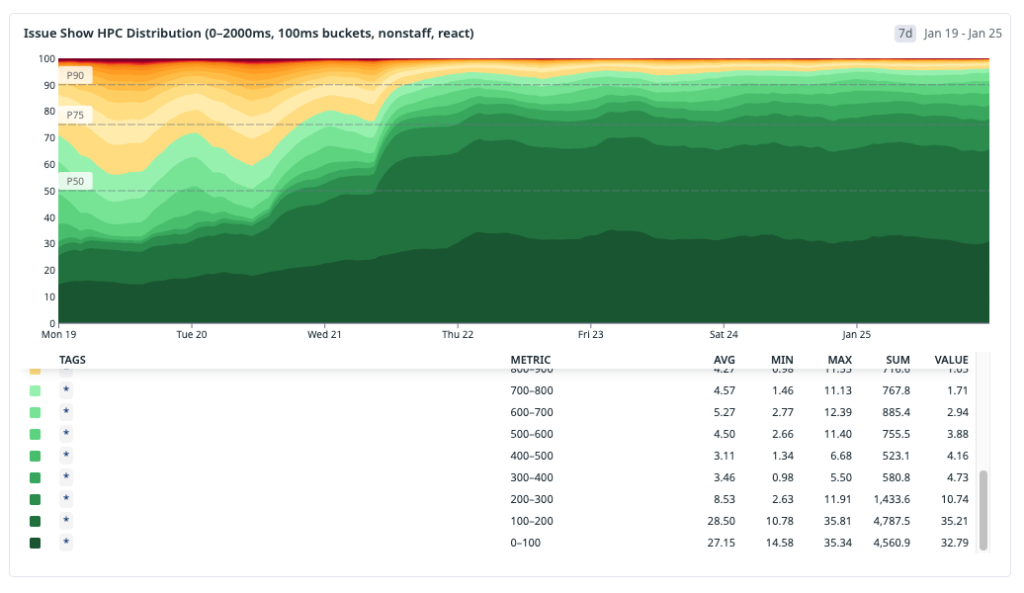
We use HPC (Highest Priority Content), an internal metric closely aligned with Web Vitals LCP, to measure when the primary content (the content users care about) on the page is first rendered. Like LCP, this is anchored to a single HTML element selected by the browser, which on issue pages is most often the issue title or the issue body. If that element is rendered quickly, the experience feels responsive even if non-critical page regions are still loading.
Operationally, we bucket navigations using HPC thresholds:
Instant: HPC < 200 ms
Fast: HPC < 1000 ms
Slow: HPC >= 1000 ms
These thresholds give us a practical model for user-perceived speed, not just raw backend latency. The <200 ms bucket maps to interactions that feel immediate in real workflows, while the <1000 ms bucket captures experiences that are still acceptable but no longer invisible to users.
This is also the point at which our measurement philosophy evolved. Historically, we dedicated significant effort to tracking the p90 and p99 of the HPC and minimizing the worst tail of the distribution. While this work remains important, it does not inherently ensure that the product feels fast for the majority of users. It is possible to enhance the p99 of the HPC while still leaving the median experience feeling sluggish.
For this initiative, we shifted focus toward distribution quality: how many navigations land in our fast and instant buckets across the whole population? The goal is not just fewer terrible outliers. It’s to make speed the default path for the majority of sessions.
The baseline: Navigation mix before we changed anything
Before implementing optimizations, we needed a clear model of how users were actually reaching issues#show (the route for viewing an issue). Treating all navigations as one class of traffic would hide the real bottlenecks.
We identified three primary navigation types:
Hard navigation: a full browser load (cold start or refresh) where we pay the full cost of network, server rendering, asset loading, JavaScript boot and React hydration.
Turbo navigation: a Rails Turbo transition that updates targeted page regions without a full reload. It avoids some hard-navigation overhead but still depends heavily on server-rendered responses.
Soft navigation (React): a client-side transition inside the existing React runtime, where we can often avoid full page bootstrap costs.
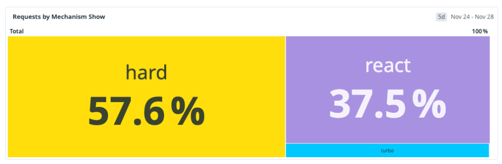
Our measured distribution at the start of the workstream was:
That distribution made one thing obvious: the dominant path was also the slowest. Any strategy focused only on React soft navigations could improve part of the experience, but it could not move overall perceived performance enough on its own.
This baseline shaped our next architecture decisions: improve the fast paths and reduce the hard-navigation penalty, because that’s where most users were seeing the most latency.
One thing to note: GitHub is still in the middle of moving from Rails-rendered pages to a React frontend. During that transition, many user journeys cross the Rails/React boundary. When that happens—for example, navigating from a Rails page into Issues—the browser often has to do a full hard navigation and cold boot. That boundary crossing is a big reason hard navigations made up the largest share of our baseline.
We expect that share of hard navigations to decrease over time as more surfaces become React-native. But we could not wait for platform migration alone to solve our problem. We started by optimizing React soft navigations first, where we had immediate architectural leverage and could ship improvements quickly.
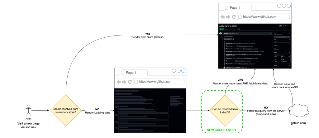
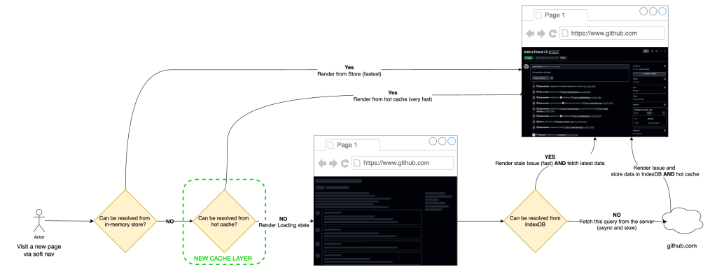
Once we aligned on the target, our strategy became clear: build a local-first application model with stale-while-revalidate. That means rendering immediately from locally available data to minimize user-visible latency, then asynchronously revalidating against the server and reconciling the UI if newer data exists.
Step 1: Client-side caching with IndexedDB
We started where we had the most leverage and where we want to move most traffic in the future: React soft navigations. In this path, the runtime is already alive, so the dominant cost is usually data fetch latency, not application boot. If we could remove network from repeated visits, we could move a large slice of traffic into the instant bucket.
Our pre-workstream analysis showed a strong repeated-access pattern: users reopen the same issues frequently during triage and collaboration loops. Based on that behavior, we estimated a potential cache-hit ratio of roughly 30% for issues#show and used that as the initial viability threshold.
The implementation was to extend our current in-memory store with a persistent client cache in IndexedDB.
Why we chose IndexedDB for this layer:
Durable browser storage that survives tab closes and browser restarts, unlike memory-only stores.
Indexed object-store model, which gives efficient key-based lookups for issue query payloads.
Larger practical quota than localStorage, making it appropriate for real working sets.
On top of that storage layer, we implemented stale-while-revalidate semantics:
Read path: on soft navigation, attempt to hydrate from local cache first and render immediately.
Revalidation path: issue a background network request for freshness and reconcile the in-memory store if data changed.
Failure behavior: when network is degraded, users still get a usable page from cache, with freshness reconciled once connectivity recovers, introducing a new graceful-degradation model.
The architectural point is that this is not “cache or correctness.” It is latency-first rendering with asynchronous consistency checks on the same navigation.
Initial production results validated the model. After broad rollout to all users, approximately 22% of React navigations became instant—up from 4% pre-launch—representing about 15% of total request volume. Observed cache-hit ratio landed around one-third (~33%), which was consistent with the earlier revisit analysis.
The main tradeoff is controlled staleness. We measured server/cache divergence at about 4.7% and treated that as an explicit operating envelope: acceptable for the perceived speed gains on soft navigations, with safeguards to limit user-visible inconsistency.
Moving the needle on cache-hit ratios
Caching is only as good as its cache-hit ratio. The IndexedDB-backed SWR (Stale-While-Revalidate) layer gave us a strong first step, but a one-third hit rate also exposed the next limitation: most navigations still arrived before the data did.
The naive answer was obvious: prefetch every likely next issue as early as possible. We explored that direction and quickly ran into the real constraint, which was not implementation complexity but capacity. On high-fanout surfaces such as issue lists, dashboards, and projects, eager prefetching amplifies request volume, creates N+1-style access patterns and pushes unnecessary compute onto the system for pages a user may never open.
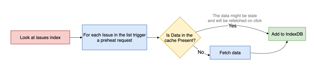
So we changed the objective. Instead of trying to make prefetched data always fresh, we optimized for a cheaper and more scalable condition: make sure some usable data is already local by the time the user clicks.
That is preheating. Preheating proactively walks high-intent issue references and prepares cache entries ahead of navigation, but it only hits the network when the issue is not already present in the client cache. If usable data already exists, preheating stops. This makes it fundamentally different from traditional preloading. It is cache-population logic, not freshness-enforcement logic.
This is an explicit tradeoff between freshness and capacity usage. We are willing to serve data that may be slightly stale if that allows the navigation itself to complete near instantaneous, because once the user opens the issue, we can still revalidate in the background and converge to the latest server state.
To support that model efficiently, we introduced an in-memory cache version in front of IndexedDB. IndexedDB gives persistence across tabs and sessions, but it is still asynchronous and therefore not free on the critical path. The in-memory layer sits between the active in-memory store and persistent storage, allowing hot issue payloads to be served synchronously without paying even the IndexedDB read cost. In practice, this removes another async boundary from soft navigation and materially increases the probability of rendering directly from memory.
Operationally, preheating is triggered from high-intent surfaces such as issue lists, dashboards, projects, and dependency views. Requests run on low-priority workers, are strictly rate-limited and are guarded by circuit breakers, so the mechanism backs off under pressure. User-initiated work always takes precedence over speculative fetches, allowing us to avoid the noisy-neighbor problem and keep the system stable while still improving cache-hit ratios for real user navigations.
The result was a large shift in distribution. After rolling out preheating broadly, instant navigations for issues#show increased to roughly 30% overall. For React navigations specifically, up to ~70% became instant. Cache-hit ratio rose to roughly 96%.
That tradeoff was acceptable. We spent a small amount of controlled background capacity to move a large percentage of real user navigations out of the network-bound path.
Expanding the fast path: Optimizing turbo and hard navigations
We were happy with the React navigation gains, but soft navigations aren’t the whole story. Even as more of GitHub moves from Rails to React, hard navigations will always exist—refreshes, new tabs, direct URLs, and inbound links. Those cold starts still matter, so we wanted cached data to help there too.
The mechanism we chose was a service worker.
A service worker is a browser-managed script that runs outside the page itself and can intercept network requests before they reach the server. Conceptually, it sits between the browser and the origin as a programmable middleman. That makes it one of the few web platform primitives that can influence hard navigations without requiring the page’s JavaScript runtime to already be active.
For issues#show, our service worker extends the same local-first model we built for React navigations. When the browser starts a navigation request for an issue page, the service worker intercepts it and checks whether the issue data is already available in local cache. If it is, the worker annotates the outgoing request with a specific header that tells the server it can skip a substantial amount of work.
When the service worker detects a cache hit, it signals to the server via a request header. From there, the navigation splits into two paths:
Cache hit path: return a thin HTML shell (layout + minimal markup + JS), and let React render from the locally cached issue payload.
Cache miss path: return the normal response (server loads data and SSRs the page).
This is a strict optimization: if the cache is cold, stale, or the service worker isn’t available, behavior falls back to the standard server-rendered path.
This had an especially strong effect on Turbo navigations, because Turbo paths are still heavily constrained by server response time. Once the service worker can signal that issue data is already present, the server spends much less time computing the application fragment, and Turbo benefits almost immediately from that reduction in backend work.
Hard-navigation gains are real, but they are less immediately visible than Turbo gains: on cache-hit hard navigations, so we trade SSR time for client-side rendering. The critical path now becomes JavaScript download and execution.
To reduce that cost, we split code by route using React.lazy and dynamic route preloading, so only the code required for the current route is fetched up front. We apply the same principle at the component level, loading only what’s necessary for the initial view and deferring non-critical modules. For example, we only fetch the issue editor bundle when a user enters edit mode, and use intent-based prefetching (like hover) to hide that latency without bloating the initial bundle.
The results
After deploying these changes, we wanted to step back and look at the cumulative impact. We analyzed the HPC metric across the entire rollout period—from the initial IndexedDB cache through preheating, in-memory layering, and the service worker—and the trend is clear and sustained: the distribution is shifting toward fast.
Rather than cherry-pick a single good week, we looked at the full window to share some concrete wins from recent months. Below are the HPC percentiles across all issues#show traffic:
P10: ~600 ms → 70 ms — the fastest navigations moved firmly into the instant bucket, well below 200 ms.
P25: ~800 ms → 120 ms — a quarter of all navigations now complete in under 120 ms, down from nearly a full second.
P50: ~1,200 ms → 700 ms — the median experience crossed below the one-second threshold, moving from the slow bucket into fast.
P75: 1,800 ms → 1,400 ms — the upper quartile dropped by over 400 ms, shrinking the long tail of perceptible latency.
P90: 2,400 ms → 2,100 ms — even the slowest navigations improved, though this tail remains the clearest signal of where further work is needed.
The pattern that stands out is the outsized improvement in the lower percentiles. P10 and P25 compressed dramatically because cached and preheated navigations now dominate that part of the distribution. The median improved meaningfully but is still shaped by cold-start traffic. And the upper tail, while better, reflects the hard-navigation paths where JavaScript boot and client rendering are now the bottleneck—exactly the area we are targeting next.
Numbers tell the optimization story, but what ultimately matters is the user impact. The video below shows what these changes feel like in practice—navigating between issues at full speed in a real session:
The work ahead
GitHub Issues is faster today than it has ever been. Across soft navigations, preheated paths, and service-worker-accelerated flows, we have materially changed the distribution of user-perceived latency and moved a much larger share of traffic into the instant bucket.
At the same time, we are not done. Cold starts that rely on SSR are still a real hurdle, especially when client boot and JavaScript execution become the dominant cost after server work is reduced.
The next phase is about moving bigger rocks. We are planning targeted rewrites of parts of our backend stack optimized explicitly for low-latency delivery and are investing in a modern UI delivery layer closer to the edge to reduce round trips and improve response time further.
Performance remains a continuous systems investment, not a one-time project. The architecture is improving, the bottlenecks are changing, and we will keep iterating until fast is the default experience across all navigation paths.
While researching a critical authentication bypass vulnerability, CVE-2026-20127, which was exploited in-the-wild, Rapid7 Labs discovered a new authentication bypass vulnerability affecting Cisco Catalyst SD-WAN Controller (formerly known as vSmart), CVE-2026-20182.
This new authentication bypass vulnerability affects the “vdaemon” service over DTLS (UDP port 12346), which is the same service that was vulnerable to CVE-2026-20127. The new vulnerability is not a patch bypass of CVE-2026-20127. It is a different issue located in a similar part of the “vdaemon” networking stack.
This impact however is the same, a remote unauthenticated attacker can leverage CVE-2026-20182 to become an authenticated peer of the target appliance, and perform privileged operations, such as injecting an attacker controlled public key into the vmanage-admin user account’s authorized SSH keys file. Once this has been performed, a remote unauthenticated attacker can login to the NETCONF service (SSH over TCP port 830) as the vmanage-admin user, and begin to issue arbitrary NETCONF commands.
CVE-2026-20182 has a CVSSv3.1 score of 10.0 (Critical), and a Common Weakness Enumeration (CWE) of CWE-287: Improper Authentication.
Technical analysis
The Cisco Catalyst SD-WAN Controller serves as the central control plane. Unlike Cisco Catalyst SD-WAN Manager, it has no web UI. Its network-reachable attack surface is narrow and depending on the configuration may expose the following ports:
Port
Protocol
Service
22
TCP
SSH (OpenSSH)
830
TCP
NETCONF over SSH
12346
UDP
vdaemon DTLS control plane
⠀
UDP port 12346 is the DTLS-over-UDP control-plane peering port used by vdaemon for inter-controller and controller-to-edge communication. It carries Overlay Management Protocol (OMP) messages including route advertisements, Transport Locations (TLOC) tables, and peer state – the entirety of the SD-WAN overlay routing fabric. Compromising this service means compromising the network.
To understand the vulnerability, we first need to understand how vdaemon authenticates control-plane peers. The protocol is a multi-phase handshake over DTLS:
After a DTLS handshake completes (which accepts any client certificate), the server sends a CHALLENGE containing 256 random bytes and a set of TLVs including Certificate Authority (CA) RSA public key components. The client must respond with a CHALLENGE_ACK, and it is during the processing of this response, in vbond_proc_challenge_ack(), that device-type-specific certificate verification occurs. Or, in the case of a “vHub” device, does not occur.
The 12-byte message header format for the vdaemon protocol is as follows:
Byte Offset
Byte Size
Field
Notes
0
1
msg_type
Low nibble = type, high nibble = version
1
1
device_info
High nibble = device_type, low nibble = flags
2
1
flags
Standard value of 0xA0
3
1
padding
Always 0x00
4 – 7
4
domain_id
Big-endian uint32
8 – 11
4
site_id
Big-endian uint32
⠀
The vdaemon protocol defines the following device types, encoded in the upper nibble of header byte 1, aka device_info:
Value
Device Type
Role
1
vEdge
Data-plane router
2
vHub
Hub router
3
vSmart
Control-plane controller
4
vBond
Orchestrator (trust anchor)
5
vManage
Management plane
6
ZTP
Zero-touch provisioning
⠀
This is the core of the vulnerability. Below is a walk through of the decompiled code from vbond_proc_challenge_ack(), which processes the CHALLENGE_ACK message sent by a connecting peer. After the DTLS handshake, the function extracts the peer’s certificate serial number and then enters device-type-specific verification (Note: edited for brevity):
We can see from the above that the function implements device-type-specific verification through a series of conditional blocks:
At [1] above, the function checks whether the connecting peer claims to be a vSmart (type 3) or vManage (type 5). If so, it enters a certificate serial number lookup via is_serial_duplicate(), which searches the local certificate database for a matching serial. At [2], if the serial is found, a duplicate-serial check via vbond_peer_dup_check() rejects the peer if a peer with that serial is already connected – preventing impersonation of existing authorized controllers.
At [3], a second verification block performs full certificate chain verification via vdaemon_dtls_verify_peer_cert(). This block executes only for specific (peer_type, local_type) pairs: vSmart-to-vSmart, vManage-to-vSmart, vManage-to-vManage, vManage-to-vBond, and vSmart-to-vBond. No pair in this block involves device type 2 (vHub). If the verification function returns a non-zero error, v18 is set to 0, and the function jumps to LABEL_179, which rejects the peer.
At [4], vEdge peers (type 1) enter hardware certificate verification via vdaemon_verify_peer_bidcert(). This path validates either a hardware TPM-based certificate (for physical vEdge routers) or a virtual edge certificate, including challenge-response signature verification and board ID validation. Failure sends the function to LABEL_179, which rejects the peer.
At [5], this is the bug, there is no “if” block matching a device type of 2 (vHub); the vHub device type simply has no verification code. The function falls through every conditional without entering any of them.
At [6], the function unconditionally sets “*(_BYTE *)(a2 + 70) = 1”, which is equivalent to ”peer->authenticated = true”, and returns success. The authenticated flag at peer struct offset 70 is the single bit that gates all subsequent message processing.
The following table summarizes the verification applied to each device type:
Device Type
Value
Verification
Result
vEdge
1
HW cert, challenge signature, board ID, OTP
Verified
vHub
2
None
Falls through to “peer->authenticated = 1”
vSmart
3
Cert chain, serial lookup, duplicate check
Verified
vBond
4
N/A (trust anchor – handled elsewhere)
–
vManage
5
Cert chain, serial lookup, duplicate check
Verified
⠀
Therefore, a remote unauthenticated attacker can bypass authentication by connecting to the vSmart DTLS port with any self-signed client certificate and claiming to be a vHub (type 2) in the CHALLENGE_ACK message. No valid credentials, no CA-signed certificate, and no knowledge of the SD-WAN deployment are required.
Looking further at the message dispatcher, we need to confirm that the CHALLENGE_ACK message can actually reach vbond_proc_challenge_ack() without prior authentication. The answer is in the pre-dispatch authentication gate in vbond_proc_msg():
We can see at [1] above, that the condition is a conjunction of negations: the incoming message is rejected only if the peer is NOT authenticated AND the message type is not one of the pre-authentication allowed types (CHALLENGE, CHALLENGE_ACK, NEW_CHALLENGE_ACK, CHALLENGE_ACK_ACK, Data, and TEAR_DOWN).
CHALLENGE_ACK (Message type 9) is explicitly in the allow list, meaning it passes this gate without authentication and reaches the vulnerable vbond_proc_challenge_ack(). This is by design; the authentication handshake must be able to proceed before the peer is authenticated.
Once the vulnerable vbond_proc_challenge_ack() sets “peer->authenticated = true” via the vHub bypass, the attacker must send a Hello message (Message type 5) to transition the peer to the UP state. The Hello handler has its own secondary authentication check:
// Case 5 (Hello) in vbond_proc_msg - line 20362
case 5:
// ...snip...
if ( *(_BYTE *)(v100 + 70) != 1 ) // <--- [2]
{
// "Received an unexpected HELLO from un-authenticated device"
        // ... cleanup and reject ...
return 0LL;
    }
// Process Hello normally - peer transitions to UP
⠀
At [2] above, the Hello handler verifies ”peer->authenticated == true” before processing. After our exploit sets this flag via the vHub bypass, Hello passes this secondary check and the peer transitions to the UP state, a fully trusted control-plane peer.
Putting all the pieces together: the attack chain is DTLS handshake (any cert) → receive CHALLENGE → send CHALLENGE_ACK with device type 2 (vHub) → authentication flag set unconditionally → send Hello → peer transitions to UP.
After establishing as an authenticated peer, the attacker has access to the full range of control-plane message types. We identified a particularly impactful post-authentication primitive: persistent SSH key injection via MSG_VMANAGE_TO_PEER (Message type 14).
The handler for message type 14 is vbond_proc_vmanage_to_peer(). Examining the decompiled code:
At [1] above, the file is opened in append mode – the attacker’s key is added alongside any existing authorized keys, avoiding disruption of legitimate access. At [2], the attacker-controlled key buffer from the message body is written directly via fputs() with no sanitization.
The key injection message body is a fixed 769-byte structure:
The leading “\n” ensures correct appending regardless of whether the existing authorized_keys file ends with a newline. The null byte terminates the string for fputs(), and the remainder is zero-padded to fill the 768-byte buffer.
Any authenticated peer, regardless of device type, can inject SSH keys into the vmanage-admin user’s authorized_keys file on vSmart. The vmanage-admin user is a specific internal, high-privileged service account used for automated communication between the management plane (vManage) and the control plane (vSmart/vBond). This converts a transient control-plane peering session into persistent, credential-independent high-privileged access.
Exploitation
In this example we will use the exploit developed by Rapid7 Labs and target a Cisco Catalyst SD-WAN Controller which has an IP address of 192.168.80.11. In our example, both the vdaemon service and the NETCONF service are bound to the same interface. The attacker will have an IP address of 192.168.80.130. In our example, the target Cisco Catalyst SD-WAN Controller appliance is running version 20.12.6.1, which was the latest available version of the 20.12.* branch at the time of writing.
To begin, the attacker loads the module in Metasploit and configures the required options.
Figure 1: Metasploit module options for cisco_sdwan_vhub_auth_bypass
⠀
The module will perform the authentication bypass and then inject an attacker controlled SSH public key into the authorized keys file for the vmanage-admin user. The module will generate a new RSA key-pair prior to exploitation, so that the attacker will inject a public key for which they have the corresponding private key.
The attacker then sets the target and runs the module.
msf6 auxiliary(admin/networking/cisco_sdwan_vhub_auth_bypass) > set RHOSTS 192.168.80.11
msf6 auxiliary(admin/networking/cisco_sdwan_vhub_auth_bypass) > run
⠀
Figure 2: Module output showing the vHub authentication bypass and SSH key injection
⠀
The attacker can now SSH into the NETCONF service over TCP port 830 by running the following command (as instructed by the exploit above).
SSH public key authentication will succeed, and the attacker will have successfully established a connection to the NETCONF service.
Figure 3: Successful SSH connection to the NETCONF service as vmanage-admin
⠀
At this point the attacker can begin to execute arbitrary NETCONF commands, for example the following “get-config” command can be run by the attacker in the NETCONF session.
The output of the get-config command is shown below.
Figure 4: NETCONF get-config output from the compromised controller
⠀
The full Metasploit module will be made available on May 27, 2026.
Remediation
Cisco has released software updates that address this vulnerability. There are no workarounds that address this vulnerability.
Customers are advised to upgrade to an appropriate fixed software release as indicated in the Fixed Software section of the Cisco Security Advisory. The following tables indicate the appropriate fixed software releases.
For additional details, please see the vendor advisory.
Vendor statement
“Cisco values the role of the security research community in helping maintain a secure ecosystem and we appreciate the collaboration with Rapid7. We have released a software update to remediate the identified vulnerability. We remain committed to transparent communication and to providing our customers with the robust security and resilience they expect.”
Rapid7 customers
Exposure Command, InsightVM and Nexpose customers will be able to assess their exposure to CVE-2026-20182 with an authenticated vulnerability check expected to be available in the May 14th, 2026 content release.
Credit
This vulnerability was discovered by Stephen Fewer, Senior Principal Security Researcher, and Jonah Burgess, Senior Security Researcher, both at Rapid7 and is being disclosed in accordance with Rapid7’s vulnerability disclosure policy.
Disclosure timeline
March 9, 2026: Rapid7 makes initial outreach to Cisco who confirms contact the same day. Rapid7 discloses the technical writeup and exploit code to Cisco.
March 11, 2026: Cisco confirms receipt of the technical writeup and exploit code and suggests a disclosure date of May 7, 2026.
March 20, 2026: Cisco confirms the vulnerability findings, and that a CVE will be reserved.
April 21, 2026: Cisco provides reserved CVE identifier and remediation guidance.
April 24, 2026: Cisco provides remediation version numbers, alignment on CWE and CVSS scoring, and requests moving disclosure date to May 14.
Imagine you build a massive corporate campus with every security control money can buy. Blast resistant doors. Biometric scanners. Guards at every entrance. Maybe something similar to the infamous Death Star. On paper, it looks fantastic. Then, somewhere along the way, somebody decides the maintenance team needs a universal key that opens every door in the building without setting off any alarms.
That certainly makes operations easier, but it also means one mistake, one compromise (like a well placed photon torpedo), or one very bad decision can unravel the whole thing.
That is basically the problem we keep running into in modern enterprise networking.
Why SD-WAN controllers create concentrated risk
This week, Rapid7 researchers Stephen Fewer and Jonah Burgess disclosed CVE-2026-20182, a maximum severity (CVSS 10.0) vulnerability in the Cisco Catalyst SD-WAN Controller. The technical details matter, and quite a bit, at that, but the bigger lesson here is even more important. This bug is a reminder that we keep designing infrastructure for efficiency first and then acting surprised when attackers go after the one component that controls everything.
To put it simply, the flaw behaves like a master key. An attacker can present themselves to the controller as a trusted network router and, if the system accepts that claim without properly validating it, they can obtain the highest level of administrative access. That is the cybersecurity version of a Jedi mind trick. The controller is effectively told to trust something it has no business trusting, as if an attacker waves a hand and says, “these are not the droids you are looking for”. And with CVE-2026-20182, the controller just nods and lets them pass.
And that becomes extremely important when you look at how these environments are built.
A decade ago, managing a global enterprise network meant touching thousands of individual routers across branch locations. It was slow, error-prone, and frankly a little miserable for the people responsible for keeping it all running. So the industry did what the industry usually does. We centralized control. We pulled the decision-making out of all those edge devices and moved it into a central controller.
From an operations standpoint, that was a huge win. I will gladly give credit where it is due. SD-WAN solved real problems.
It also created a very attractive target.
Why central management platforms are attractive targets
Once you move the brains of the operation into a single place, that place becomes the thing an attacker wants most. Compromising one branch router is useful. Compromising the controller that manages the entire estate is a very different conversation. Now you are talking about the ability to reroute traffic, intercept communications, push malicious configuration, or simply break connectivity across the whole organization.
That is the real paradox here. The same architecture that gives defenders scale and simplicity can also give attackers a single point of catastrophic leverage.
A few years ago, finding and exploiting a quiet authentication bypass in a core networking appliance was mostly the work of highly capable nation-state teams. That is not the world we live in anymore, especially as AI makes exploitation faster to analyze, adapt, and operationalize. The reality of it is that offensive tradecraft does not stay exclusive for very long. It gets copied, adapted, automated, and eventually handed down to groups with very different goals.
For nation-state operators, a bug like this (as seen with the actively exploited CVE-2026-20127) is ideal for pre positioning. They are usually not looking for a smash and grab. They want persistence. They want access that blends in. They want to sit in the right place long enough to observe, influence, and pivot when the time is right. An SD-WAN controller is a great place to do that, because it lives in the middle of trust relationships most organizations rarely question.
For ransomware groups, the value proposition is even more obvious. If you can compromise central infrastructure, you do not have to fight for access to one system at a time. You are standing on the control plane of the enterprise, facing a dramatically lower barrier to initial access and large-scale disruption.
Now, to be fair, not every bug turns into internet wide exploitation overnight and not every vulnerability becomes a one click offensive toolkit. We should avoid sensationalizing that part. But we should also be honest about where the pressure is today. Attackers have become very good at turning central infrastructure weaknesses into high impact operations.
What defenders should do now
First, bugs like this are going to happen again. As long as we keep building extremely complex systems to manage global infrastructure, there will be flaws. That is not cynicism. That is just reality.
Second, organizations need to stop assuming that trusted administrative systems are inherently safe just because they sit in the middle of the network and have important sounding names. If your controller is compromised, what happens next? What can it reach? What can it change? How much of the enterprise can it influence without another human ever noticing?
That blast radius question is the one that matters.
Defending against this kind of problem requires more than patching, even though patching absolutely needs to happen. It means building environments that can survive the compromise of a critical management system. Network segmentation matters. Monitoring administrative traffic matters, whether that is handled internally or through an MDR provider that can help catch suspicious behavior before it turns into a much larger problem. Tight control over outbound communications from infrastructure devices matters. So does limiting which systems are allowed to talk to the controller in the first place.
In other words, we need to design with the assumption that even high trust infrastructure can fail in ugly ways.
The immediate guidance for defenders is straightforward: apply the vendor supplied patches for Cisco Catalyst SD-WAN Controllers as quickly as possible. That is the first move, not the last one.
The longer term lesson for leadership is bigger than this one vulnerability. Efficiency is great right up until it creates unquestioned authority in a single device or platform. When that happens, you have not removed complexity. You have concentrated risk.
And attackers have noticed.
Register for Rapid7’s upcoming webinar on CVE-2026-20182 here.
In back-to-back sessions at the start of the 2026 Linux Storage,
Filesystem, Memory Management, and BPF Summit (which spilled over into
a third slot), the atomic-buffered-writes
feature was discussed. In the first session, Pankaj Raghav and Andres
Freund set the stage with an introduction to the problem, along with a use
case for its solution: the PostgreSQL database system. In the second, Ojaswin Mujoo
described a potential way forward for the feature using an approach based
on writethrough, which effectively means that the kernel immediately writes
the data to disk instead of waiting for writeback from the page cache to occur. As might be
expected, there was quite a bit of discussion among the assembled
filesystems and storage developers during the combined sessions for those
tracks.
Greg Kroah-Hartman has announced the release of the 7.0.7, 6.18.30, and 6.12.88 stable kernels. These kernels do
not include a patch for the Fragnesia local-privilege-escalation exploit that came to light on
May 13, but do include many other important fixes throughout the
tree. Users are, as always, advised to upgrade.
The kernel’s reverse-mapping machinery is charged with locating the
page-table entries that refer to a given page in memory. The reverse
mapping of anonymous pages is handled differently than for file-backed
pages. The kernel’s implementation of reverse mapping for anonymous pages
is, according to Lorenzo Stoakes in his proposal
for a memory-management-track session at the 2026 Linux Storage,
Filesystem, Memory Management, and BPF Summit, “a very broken
abstraction“, due to its complexity. It also has some performance
problems. Stoakes was there to present, in raw form, a proposed
replacement that he calls a “COW context”.
At Cloudflare, we are heavy users of ClickHouse, an open-source analytical database management system. We redesigned one of our largest ClickHouse tables to add a column to the partitioning key. The change enabled per-tenant retention on a table that serves hundreds of internal teams. The design went through several rounds of revision and review with engineers across multiple teams before we landed on the final approach. But a few weeks after rollout, the jobs that produce most of Cloudflare’s bills were running up against their hard daily deadline.
All the usual suspects looked clean: I/O, memory, rows scanned, parts read. Everything we would normally check when a ClickHouse query is slow appeared to be normal. The problem turned out to be lock contention in query planning, something we’d never had reason to look for before.
This is the story of how this migration exposed a hidden bottleneck in ClickHouse’s internals, and the patches we wrote to fix it.
The setup: a petabyte-scale analytics platform
We use ClickHouse to store over a hundred petabytes of data across a few dozen clusters. To simplify onboarding for our many internal teams, we built a system called “Ready-Analytics” in early 2022.
The premise is simple: instead of designing new tables, teams can stream data into a single, massive table. Datasets are disambiguated by a namespace, and each record uses a standard schema (e.g., 20 float fields, 20 string fields, a timestamp, and an indexID).
In ClickHouse, the way data is sorted is crucial to query performance. This is where the indexID comes into play. It’s a string field, which forms part of the primary key, meaning that every individual namespace can have its data sorted in a way that is optimal for the queries the owners of that namespace expect to be running. Altogether, we end up with a primary key that looks like this: (namespace, indexID, timestamp).
This system is popular, with hundreds of applications using it. It had already grown to more than 2PiB of data by December 2024, and an ingestion rate of millions of rows per second. But it had one critical flaw: its retention policy.
The problem: one retention policy to rule them all
Cloudflare has been using ClickHouse for many years, since before it had native Time-to-Live (TTL) features. Consequently, we built our own retention system based on partitioning. The Ready-Analytics table was partitioned by day, and our retention job simply dropped partitions older than 31 days.
This “one-size-fits-all” 31-day retention was a major limitation. Some teams needed to store data for years due to legal or contractual obligations, while others needed only a few days. This restriction meant these use cases couldn’t use Ready-Analytics and had to opt for a conventional setup, which has a far more complex onboarding process.
We needed a new system that allowed per-namespace retention.
The solution: a new partitioning scheme
We considered two main approaches:
A Table-per-Namespace: This would naturally solve the retention problem but would require significant new automation to manage thousands of tables on demand.
A New Partitioning Key: We could change the partitioning key from just (day) to (namespace, day).
We chose the second option. This would allow our existing retention system to continue managing partitions, but now with per-namespace granularity.
We knew this would increase the total number of data parts in the table, but we made a key assumption: since every query is filtered by a specific namespace, the number of parts read by any single query shouldn’t change. We believed this meant performance would be unaffected.
This shows how we changed the partitioning, allowing us to cheaply drop data for a single namespace
This new system also allowed us to build a sophisticated storage management layer. Using themax-min fairness algorithm, we could set a target disk utilization (e.g., 90%) and automatically “share” available space. Namespaces using less than their fair share would cede their unused capacity to those that needed more. This allowed us to confidently run our clusters at 90% utilization.
We began the migration in January 2025. Using ClickHouse’s Merge table feature, we combined the old and new tables, writing all new data to the new partitioned table while the old data aged out.
The mystery: when billing starts to break
Two months later, in late March 2025, our billing team reported that their daily aggregation jobs were slowing down. These jobs are time-critical; if they don’t finish, bills don’t go out. The jobs were getting progressively slower, and we were approaching a deadline.
We investigated, but none of the usual suspects were to blame. I/O was fine. Memory was fine. The metrics for individual queries showed they were not reading more data or more parts than before. Our initial assumption seemed correct, yet the system was grinding to a halt.
It took several days before we even had a theory. Finally, we made a plot of query duration against the total part count in the cluster. The correlation was undeniable.
Average SELECT Query Durations on the Ready Analytics ClickHouse Cluster, showing progressive performance degradation.
Linear Growth in Total Data Part Count per Table Replica, following the new (namespace, day) partitioning scheme.
But why? If we weren’t reading the extra parts, why did their mere existence slow us down?
The investigation: hunting bottlenecks with flame graphs
We turned to ClickHouse’s built-in trace_log to generate flame graphs. This is a built-in table that records traces from the running ClickHouse server. It not only includes traces of what code is being executed, but it associates these with specific users, query IDs and other metadata, meaning you can filter down to quite precise sets of events if necessary. In our case, we wanted to look specifically at leaf SELECT queries. This was easy thanks to the available metadata in this table.
The first CPU-based flame graph quickly confirmed our suspicion: a huge amount of time was being spent in query planning. This is the phase before execution when ClickHouse decides which parts to read.
Flame graph showing that 45% of leaf query CPU time is spent filtering a vector of parts based on the partition ID
The flame graph was clear: 45% of the sampled CPU time was being spent in a single function called filterPartsByPartition.
Our first attempt at a fix was a small patch to this exact code path. The planner evaluates heuristics to prune parts, and we believed they weren’t being evaluated in the optimal order for our table. Our patch changed the order, yielding a small 5% improvement. We were on the right path, but we’d missed the real problem.
We had been generating “CPU” traces, which only sample active threads. We switched to “Real” traces, which sample all threads, including those that are inactive or waiting. The new flame graph was a revelation.
Flame graph showing that more than half of leaf query duration is spent waiting for a mutex that protects the list of active parts
The problem wasn’t CPU-bound work; it was massive lock contention. More than half of our query duration was spent waiting to acquire a single mutex (MergeTreeData) that protects the table’s list of parts. To plan a query, every single thread had to:
Acquire an exclusive lock on this mutex.
Make a complete copy of the list of all parts in the table.
Release the lock.
Filter that list down to the relevant parts.
With tens of thousands of parts and hundreds of concurrent queries, they were all just standing in a single-file line.
The fixes: a trio of patches
This insight helped us plan a series of optimizations to alleviate these hotspots. As with all the patches we make to ClickHouse, we try to make them generic, and eventually get them contributed to the upstream codebase. This makes it easier for us to maintain our fork, and means the community benefits from the changes we make too!
Optimization 1: use a shared lock
The query planner doesn’t modify the parts list; it just reads it. It had no business using an exclusive lock.
The Fix: We modified the code to acquire a shared lock (std::shared_lock) instead. This allowed all query planners to enter the critical section concurrently.
The Result: A massive, immediate drop in query duration. The lock contention vanished.
Immediate Impact of the Shared Lock Optimization (Optimization 1) on Average SELECT Query Durations, demonstrating the resolution of lock contention.
Optimization 2: stop copying the vector
Performance was significantly better, but still not back to baseline. We went back to the trace log and made another ‘Real’ flame graph.
Flame graph showing that we spend a quarter of leaf query duration copying the vector of all parts, and another quarter filtering through it (copying again).
The new flame graph showed the bottleneck had simply moved. Now, time was being spent copying the giant vector of parts, even with the shared lock. Intuitively, copying a vector sounds cheap, but when it contains tens of thousands of elements, and you do it hundreds of times a second, it adds up.
The Fix: We deferred the copy entirely. We created a “shared copy” of the parts list. Read-only operations (like query planning) just read from this copy. Any operation that modifies the set of parts (like a new insert) regenerates the cache. Planners now only copy the filtered list of parts they actually need.
The Result: Another significant performance improvement.
Further Performance Improvement After Rolling Out the Vector Copy Optimization (Optimization 2).
After seeing these massive savings internally, we decided to bring these changes to the community. After some small design iterations with the maintainers at ClickHouse Inc., we got the changes merged underPR #85535. They have been available since ClickHouse version 25.11.
Optimization 3: binary search for parts
We’re still not done. As part counts grow, performance still degrades, just much more slowly. The correlation with part count was still there. Coming back to this after a few months, a new flame graph (looking the same as Figure 3) shows the time is spent in the filtering code path (the one we tried to fix first). This code performs a linear scan over all parts, evaluating predicates against each one. Over a few months, we were back to select durations from before the optimizations.
But we know this list of parts is sorted by the partitioning key. Remember that the first column of the partition key is namespace, which the vast majority of queries filter on, because it identifies the “tenant.” How can we make use of this?
The Fix: We implemented a binary search based on the namespace part of the partition ID. This works because the vector is sorted, so you can filter out a lot of the entries without actually looking at them. This is particularly effective since the namespace is the first part of that sorting key. After this first-pass of binary search, we have a much smaller range of parts we need to examine, and for those we still step through each one, applying the same logic as before to exclude parts based on other conditions.
The Result: After deploying this patch in March 2026, query durations dropped by 50% (see Figure 8). More importantly, this finally breaks correlation of query durations with the number of parts. Unfortunately, this solution doesn’t generalize that well for arbitrary query conditions (e.g. conditions such as namespace in (5,10)). We are looking into more generic approaches like extending the query condition cache to cover part filtering.
Sustained Latency Reduction Following the Implementation of Binary Search for Part Pruning (Optimization 3).
An uneasy truce
These optimizations resolved the immediate crisis with the billing system. But this journey exposed the deep, non-obvious costs of our partitioning choice.
Other problems remain. In this blog post we’ve only described the problems increasing part counts had on our select durations, but it has also caused problems for ZooKeeper, which tracks metadata for all the parts in ClickHouse. Perhaps one day we’ll tell the story of the 100 gigabyte ZooKeeper cluster.
We’ve bought ourselves significant breathing room, but the fundamental question remains: Was this partitioning scheme the right long-term choice? Or will we eventually need to bite the bullet and move to a different architecture? For now, our patches are holding, but the experience was a clear example of how even a well-planned change can fall victim to incorrect assumptions.
When the billing team first reported this problem we had 30,000 parts per replica. The part rate never stopped growing, and a year later we hit 160k parts per replica, but query durations have been stable thanks to the optimizations we made here.
At Cloudflare, we solve complex engineering problems at a massive scale. If the debugging and optimizations we described here sound like the type of challenge you’re looking for, check out some of the open roles we are hiring for.
Минавала ли ви е през ума мисълта, че в музиката вече всичко е измислено? Че не може да се появи нещо, което не прилича на нищо досега? Че изкуственият интелект е способен да генерира произведения, не по-лоши от преобладаващата посредственост, и трудът на много музиканти може да стане излишен? Мечтаете ли си нещо да разтърси света на музиката, така че тя отново да започне да вдъхновява, да провокира, изобщо – да дава смисъл? Ако да, може би има надежда. Ако харесвате музика, която бяга от клишетата,
до вас вече може да е достигнала обсесията по канадското дуо Angine de poitrine.
В случай че не е – сега ще наваксаме.
На френски името на групата означава ангина пекторис – медицинско състояние, по-известно като стенокардия или гръдна жаба. За анонимността на членовете на групата допринасят не само псевдонимите им (Khn de poitrine и Klek depoitrine), а и чудатите костюми на черни и бели точки, които скриват лицата им. Музикантите свирят на струнен инструмент с два грифа (китара и бас) и барабани. Khn използва босите си (но изрисувани на точки) стъпала, за да управлява ефекти като например лууп – записване и повтаряне на определени пасажи, върху които се свирят други.
Три месеца по-късно видеото е гледано (или поне отворено) над 14 млн. пъти, а YouTube изобилства от влогърски реакции на музиката на дуото. Екстравагантните канадци са почетени дори от Google – веднъж, когато търсех информация за Angine de poitrine, екранът на компютъра ми изненадващо се обсипа с черни точки.
Какво има между полутоновете?
Най-интересното в Angine de poitrine обаче не е външният им вид, нито анонимността им, а микротоналната им музика. За да разберем обаче какво е микротоналност, трябва да си припомним какво сме учили за тоновете.
Нека си представим клавиатурата на едно пиано. Ако започнем от произволен тон, например до, до същия тон в следващата октава (в случая – горното до) има общо 12 тона и полутона. Толкова е сборът на клавишите – седем бели плюс пет черни. Струнните и духовите инструменти също използват тази скала от 12 тона и полутона. Почти всички произведения в западната музикална традиция, които са ни известни, независимо от жанра им, са създадени върху нейната основа.
Ами ако някой изсвири тон, който е между до и най-близкия полутон, примерно, до диез? Обикновено това означава, че или инструментът не е настроен вярно, или човекът свири фалшиво.
Освен ако не става дума за микротонална музика.
Микротоновете са именно тоновете, които са между полутоновете. В микротоналната музика те не се възприемат като фалшиви, а имат право на съществуване. Микротоналностите не се свеждат до познатите ни 12 тона и полутона, а са изградени на други принципи.
На колко части, освен на две, може да се раздели един тон? Може да има 1/4 или 1/3 тон, но също и 1/17 например или каквато дроб ви хрумне. А може и разстоянието между два съседни тона да е различно от общоприетото. Защото тоновете са спектър – като цветовете. И преливането между тях е плавно. Затова и е практически невъзможно за човешкия глас, както и за голяма част от музикалните инструменти (освен може би издаващите дигитален звук) да постигнат абсолютно чисти тонове – те винаги се колебаят повече или по-малко около точния тон.
Angine de poitrine не са откривателите на микротоналността.
Тя съществува отдавна. Характерна е например за традиционната тайландска музика, в която се използва скала от седем тона на приблизително равни интервали, но различни от тези, с които сме свикнали.
Може да намерим микротонове на различни места по света, включително наблизо. Те са характерни и за турската музика, а не са съвсем чужди и на българския фолклор. Като се замислим, инструменти като гайдата и гъдулката, както и някои техники на народно пеене доста бягат от „правилните“ тонове. Което не е техен недостатък – напротив, в това им е чарът.
Впрочем микротонални инструменти се продават, и то не само фолклорни. При наличие на желание (и достатъчно средства) човек може да се снабди с микротонални китари, баскитари, струнни инструменти с два грифа като на Angine de poitrine и какво ли още не. Има дори микротонални пиана с подредби на клавишите от странни по-странни. Друг е въпросът, че всеки струнен инструмент, който няма прагчета, може да се използва за микротонална музика.
Откъде се вземат „правилните“ тонове?
Странното всъщност не е, че има микротонална музика. По-любопитният въпрос е:
след като тоновете са спектър, защо огромната част от музиката е създадена върху системата от октави с 12 полутона на равни интервали един от друг?
Тази система, наречена равномерна темперация, е създадена в края на Ренесанса и зората на Новото време – публикувана е от Джовани Лафранко през 1533 г. Тя изразява общата нагласа на епохата всичко да се подчинява на ясни рационални правила.
След като равномерната темперация достига до Германия, в нея е въведен още по-строг ред. Йохан Себастиан Бах „постановява“ кои комбинации между тоновете са „добри“, тоест звучат хармонично, а не са в дисонанс. Това са мажорните и минорните тоналности (които стават основа на класическата музика, а и на огромна част от съвременната). Така, ако ползвате само белите клавиши на пианото и започнете от до, ще изсвирите гамата в до мажор, а ако започнете от ла – в ла минор. През 1722 г. Бах създава цикъла си „Добре темперирано пиано“, включващ прелюдии и фуги в мажор и минор, започващи от всеки от 12-те тона и полутона – общо 24 (12 мажорни и още толкова минорни). Двайсет и две години по-късно композира втора част на цикъла, също от 24 произведения.
Кое е вярното ла?
Освен че през Новото време тоновете са подредени в определени интервали и се определя кои са правилните хармонични комбинации между тях, как се решава какви да са самите тонове? Класическият помощник за настройване на музикални инструменти е камертонът, който по традиция издава тона ла. Честотата на тоновете се измерва в херцове, а ла на т.нар. първа октава е 440 херца.
Невинаги обаче е било така – стандартът от 440 херца е въведен чак в края на 30-те години на XX век, а е окончателно одобрен от Международната организация по стандартизация през 50-те. Ала и до днес не всички са съгласни, че 440 са правилните херцове. Битува и схващането, че по-добротола е с честота 432 херца (т.нар. строй на Верди – на името на композитора Джузепе Верди), тоест звучи малко по-ниско. Било защото за „виновник“ за 440-те херца се смята Гьобелс, било заради убеждението, че тонът, издаван на 432 херца, е по-естествен, по-топъл и по-близък до Вселената, било и поради двата аргумента. Съществуват и 432-херцови камертони, както и оркестри (включително български), свирещи в строя на Верди.
Но както хората не са знаели колко е часът, преди да имат часовници, така и не са можели да определят каква е честотата на един тон, преди да се появят уреди, с които да се измерва тя. Така че в миналото височината на един и същи тон е варирала чувствително. За ла-то има данни, че се е движило между 309 и 455,3 херца, което е сериозна разлика от близо шест полутона.
На бунт срещу тоналността
Микротоналната музика е преоткрита в края на XIX и началото на ХХ век. Не е сигурно кой е създателят на термините микротон и микротоналност. Въвежда ги или ирландската музикантка, теософка и поетеса Мод Маккарти, която е била повлияна от индийската музика, или мексиканският композитор Хулиан Карийо.
Този период е характерен с критика на модерността и на всичко, свързано с нея – научния прогрес, рационалността, капиталистическите отношения. Критиката е както от леви позиции (работниците са сведени до винтчета на машина), така и от дясноаристократични – капитализмът премахва старите йерархии заедно с ценностите, върху които се основават те. В заключението на книгата си „Протестантската музика и духът на капитализма“ германският социолог Макс Вебер говори за „стоманената клетка на бъдещето“.
Тази критика намира израз и в изкуството – чрез стилове като експресионизма, които си поставят за цел да разчупят класическите рационални и подредени форми. Възниква атоналната музика на композитори като Арнолд Шьонберг и Албан Берг, която стъпва на равномерната темперация от 12 тона и полутона, но отрича доминиращите мажорни и минорни тоналности. Преоткриването на микротоновете е част от същата тенденция на бунт срещу класическите правила.
Защо Angine de poitrine стават вайръл точно сега?
Има периоди, в които технологиите и креативността не са врагове. 70-те години на ХХ век например са такова време за музиката – в жанрове от диското до прогресиврока се създават звуци и ефекти, които не са съществували преди. Нови стилове възникват и в следващите десетилетия. В наши дни обаче технологиите като че ли се използват не толкова за да се създава нещо интересно, колкото за улеснение. Вече дори не се налага един музикант да умее да пее вярно – гласът може да бъде софтуерно коригиран даже в реално време, на концерт на живо. Коригираните, неестествено правилни гласове са вокалният еквивалент на разкрасяващите лицата и телата софтуерни филтри и на козметичната хирургия, произвеждаща хора без бръчки, но и без естествени мимики. Не че няма и талантливи изключения, но като че ли това е нормата.
Angine de poitrine не е първата микротонална група, нито единствената – такива са например и King Gizzard & The Lizard Wizard, The Mercure Tree и др. В сравнение с тях канадското дуо успява да направи впечатление и с екстравагантния си външен вид, и с използването на комплексни неравноделни ритми (на моменти напомнящи тези в българския фолклор), но и с това, че прави всичко по силите си да не прилича на нищо друго – и в музикално, и в сценично отношение, – доколкото това изобщо е възможно.
„Музиката е пространството между нотите“, казва Клод Дебюси.
Френският композитор има предвид тишината. Но нотите обозначават тонове, а между познатите ни тонове се крият и други – микротонове. Съжителстваме с тях, без дори да ги забележим.
Във време, в което бъдещето на музиката, както и на много други сфери изглежда застрашено от изкуствения интелект, Angine de poitrine ни връщат към въпроса от какво всъщност е направена музиката. Ако я разглобим до съставните ѝ части, ако видим какво има между тоновете, може би музиката има бъдеще. Може би ще успеем да я създадем по някакъв нов начин. Е, не точно аз, но по-музикални от мен представители на човечеството.
The collective thoughts of the interwebz
Manage Consent
To provide the best experiences, we use technologies like cookies to store and/or access device information. Consenting to these technologies will allow us to process data such as browsing behavior or unique IDs on this site. Not consenting or withdrawing consent, may adversely affect certain features and functions.
Functional
Always active
The technical storage or access is strictly necessary for the legitimate purpose of enabling the use of a specific service explicitly requested by the subscriber or user, or for the sole purpose of carrying out the transmission of a communication over an electronic communications network.
Preferences
The technical storage or access is necessary for the legitimate purpose of storing preferences that are not requested by the subscriber or user.
Statistics
The technical storage or access that is used exclusively for statistical purposes.The technical storage or access that is used exclusively for anonymous statistical purposes. Without a subpoena, voluntary compliance on the part of your Internet Service Provider, or additional records from a third party, information stored or retrieved for this purpose alone cannot usually be used to identify you.
Marketing
The technical storage or access is required to create user profiles to send advertising, or to track the user on a website or across several websites for similar marketing purposes.