Post Syndicated from Veena Vasudevan original https://aws.amazon.com/blogs/big-data/amazon-emr-serverless-supports-larger-worker-sizes-to-run-more-compute-and-memory-intensive-workloads/

Amazon EMR Serverless allows you to run open-source big data frameworks such as Apache Spark and Apache Hive without managing clusters and servers. With EMR Serverless, you can run analytics workloads at any scale with automatic scaling that resizes resources in seconds to meet changing data volumes and processing requirements. EMR Serverless automatically scales resources up and down to provide just the right amount of capacity for your application.

We are excited to announce that EMR Serverless now offers worker configurations of 8 vCPUs with up to 60 GB memory and 16 vCPUs with up to 120 GB memory, allowing you to run more compute and memory-intensive workloads on EMR Serverless. An EMR Serverless application internally uses workers to execute workloads. and you can configure different worker configurations based on your workload requirements. Previously, the largest worker configuration available on EMR Serverless was 4 vCPUs with up to 30 GB memory. This capability is especially beneficial for the following common scenarios:

• Shuffle-heavy workloads
• Memory-intensive workloads

Let’s look at each of these use cases and the benefits of having larger worker sizes.

Benefits of using large workers for shuffle-intensive workloads

In Spark and Hive, shuffle occurs when data needs to be redistributed across the cluster during a computation. When your application performs wide transformations or reduce operations such as join, groupBy, sortBy, or repartition, Spark and Hive triggers a shuffle. Also, every Spark stage and Tez vertex is bounded by a shuffle operation. Taking Spark as an example, by default, there are 200 partitions for every Spark job defined by spark.sql.shuffle.partitions. However, Spark will compute the number of tasks on the fly based on the data size and the operation being performed. When a wide transformation is performed on top of a large dataset, there could be GBs or even TBs of data that need to be fetched by all the tasks.

Shuffles are typically expensive in terms of both time and resources, and can lead to performance bottlenecks. Therefore, optimizing shuffles can have a significant impact on the performance and cost of a Spark job. With large workers, more data can be allocated to each executor’s memory, which minimizes the data shuffled across executors. This in turn leads to increased shuffle read performance because more data will be fetched locally from the same worker and less data will be fetched remotely from other workers.

Experiments

To demonstrate the benefits of using large workers for shuffle-intensive queries, let’s use q78 from TPC-DS, which is a shuffle-heavy Spark query that shuffles 167 GB of data over 12 Spark stages. Let’s perform two iterations of the same query with different configurations.

The configurations for Test 1 are as follows:

• Size of executor requested while creating EMR Serverless application = 4 vCPUs, 8 GB memory, 200 GB disk
• Spark job config:
  • spark.executor.cores = 4
  • spark.executor.memory = 8
  • spark.executor.instances = 48
  • Parallelism = 192 (spark.executor.instances * spark.executor.cores)

The configurations for Test 2 are as follows:

• Size of executor requested while creating EMR Serverless application = 8 vCPUs, 16 GB memory, 200 GB disk
• Spark job config:
  • spark.executor.cores = 8
  • spark.executor.memory = 16
  • spark.executor.instances = 24
  • Parallelism = 192 (spark.executor.instances * spark.executor.cores)

Let’s also disable dynamic allocation by setting spark.dynamicAllocation.enabled to false for both tests to avoid any potential noise due to variable executor launch times and keep the resource utilization consistent for both tests. We use Spark Measure, which is an open-source tool that simplifies the collection and analysis of Spark performance metrics. Because we’re using a fixed number of executors, the total number of vCPUs and memory requested are the same for both the tests. The following table summarizes the observations from the metrics collected with Spark Measure.

As seen from the table, there is a significant difference in performance due to shuffle improvements. Test 2, with half the number of executors that are twice as large as Test 1, ran 29.44% faster, with 1.97 times more shuffle data fetched locally compared to Test 1 for the same query, same parallelism, and same aggregate vCPU and memory resources. Therefore, you can benefit from improved performance without compromising on cost or job parallelism with the help of large executors. We have observed similar performance benefits for other shuffle-intensive TPC-DS queries such as q23a and q23b.

Recommendations

To determine if the large workers will benefit your shuffle-intensive Spark applications, consider the following:

• Check the Stages tab from the Spark History Server UI of your EMR Serverless application. For example, from the following screenshot of Spark History Server, we can determine that this Spark job wrote and read 167 GB of shuffle data aggregated across 12 stages, looking at the Shuffle Read and Shuffle Write columns. If your jobs shuffle over 50 GB of data, you may potentially benefit from using larger workers with 8 or 16 vCPUs or spark.executor.cores.

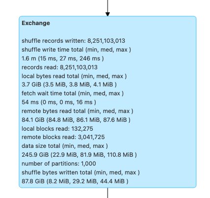
• Check the SQL / DataFrame tab from the Spark History Server UI of your EMR Serverless application (only for Dataframe and Dataset APIs). When you choose the Spark action performed, such as collect, take, showString, or save, you will see an aggregated DAG for all stages separated by the exchanges. Every exchange in the DAG corresponds to a shuffle operation, and it will contain the local and remote bytes and blocks shuffled, as seen in the following screenshot. If the local shuffle blocks or bytes fetched is much less compared to the remote blocks or bytes fetched, you can rerun your application with larger workers (with 8 or 16 vCPUs or spark.executor.cores) and review these exchange metrics in a DAG to see if there is any improvement.

• Use the Spark Measure tool with your Spark query to obtain the shuffle metrics in the Spark driver’s stdout logs, as shown in the following log for a Spark job. Review the time taken for shuffle reads (shuffleFetchWaitTime) and shuffle writes (shuffleWriteTime), and the ratio of the local bytes fetched to the remote bytes fetched. If the shuffle operation takes more than 2 minutes, rerun your application with larger workers (with 8 or 16 vCPUs or spark.executor.cores) with Spark Measure to track the improvement in shuffle performance and the overall job runtime.

Time taken: 177647 ms

Scheduling mode = FIFO
Spark Context default degree of parallelism = 192

Aggregated Spark stage metrics:
numStages => 22
numTasks => 10156
elapsedTime => 159894 (2.7 min)
stageDuration => 456893 (7.6 min)
executorRunTime => 28418517 (7.9 h)
executorCpuTime => 20276736 (5.6 h)
executorDeserializeTime => 326486 (5.4 min)
executorDeserializeCpuTime => 124323 (2.1 min)
resultSerializationTime => 534 (0.5 s)
jvmGCTime => 648809 (11 min)
shuffleFetchWaitTime => 340880 (5.7 min)
shuffleWriteTime => 245918 (4.1 min)
resultSize => 23199434 (22.1 MB)
diskBytesSpilled => 0 (0 Bytes)
memoryBytesSpilled => 0 (0 Bytes)
peakExecutionMemory => 1794288453176
recordsRead => 18696929278
bytesRead => 77354154397 (72.0 GB)
recordsWritten => 0
bytesWritten => 0 (0 Bytes)
shuffleRecordsRead => 14124240761
shuffleTotalBlocksFetched => 5571316
shuffleLocalBlocksFetched => 117321
shuffleRemoteBlocksFetched => 5453995
shuffleTotalBytesRead => 158582120627 (147.7 GB)
shuffleLocalBytesRead => 3337930126 (3.1 GB)
shuffleRemoteBytesRead => 155244190501 (144.6 GB)
shuffleRemoteBytesReadToDisk => 0 (0 Bytes)
shuffleBytesWritten => 156913371886 (146.1 GB)
shuffleRecordsWritten => 13867102620

Benefits of using large workers for memory-intensive workloads

Certain types of workloads are memory-intensive and may benefit from more memory configured per worker. In this section, we discuss common scenarios where large workers could be beneficial for running memory-intensive workloads.

Data skew

Data skews commonly occur in several types of datasets. Some common examples are fraud detection, population analysis, and income distribution. For example, when you want to detect anomalies in your data, it’s expected that only less than 1% of the data is abnormal. If you want to perform some aggregation on top of normal vs. abnormal records, 99% of the data will be processed by a single worker, which may lead to that worker running out of memory. Data skews may be observed for memory-intensive transformations like groupBy, orderBy, join, window functions, collect_list, collect_set, and so on. Join types such as BroadcastNestedLoopJoin and Cartesan product are also inherently memory-intensive and susceptible to data skews. Similarly, if your input data is Gzip compressed, a single Gzip file can’t be read by more than one task because the Gzip compression type is unsplittable. When there are a few very large Gzip files in the input, your job may run out of memory because a single task may have to read a huge Gzip file that doesn’t fit in the executor memory.

Failures due to data skew can be mitigated by applying strategies such as salting. However, this often requires extensive changes to the code, which may not be feasible for a production workload that failed due to an unprecedented data skew caused by a sudden surge in incoming data volume. For a simpler workaround, you may just want to increase the worker memory. Using larger workers with more spark.executor.memory allows you to handle data skew without making any changes to your application code.

Caching

In order to improve performance, Spark allows you to cache the data frames, datasets, and RDDs in memory. This enables you to reuse a data frame multiple times in your application without having to recompute it. By default, up to 50% of your executor’s JVM is used to cache the data frames based on the property spark.memory.storageFraction. For example, if your spark.executor.memory is set to 30 GB, then 15 GB is used for cache storage that is immune to eviction.

The default storage level of cache operation is DISK_AND_MEMORY. If the size of the data frame you are trying to cache doesn’t fit in the executor’s memory, a portion of the cache spills to disk. If there isn’t enough space to write the cached data in disk, the blocks are evicted and you don’t get the benefits of caching. Using larger workers allows you to cache more data in memory, boosting job performance by retrieving cached blocks from memory rather than the underlying storage.

Experiments

For example, the following PySpark job leads to a skew, with one executor processing 99.95% of the data with memory-intensive aggregates like collect_list. The job also caches a very large data frame (2.2 TB). Let’s run two iterations of the same job on EMR Serverless with the following vCPU and memory configurations.

Let’s run Test 3 with the previously largest possible worker configurations:

• Size of executor set while creating EMR Serverless application = 4 vCPUs, 30 GB memory, 200 GB disk
• Spark job config:
  • spark.executor.cores = 4
  • spark.executor.memory = 27 G

Let’s run Test 4 with the newly released large worker configurations:

• Size of executor set in while creating EMR Serverless application = 8 vCPUs, 60 GB memory, 200 GB disk
• Spark job config:
  • spark.executor.cores = 8
  • spark.executor.memory = 54 G

Test 3 failed with FetchFailedException, which resulted due to the executor memory not being sufficient for the job.

Also, from the Spark UI of Test 3, we see that the reserved storage memory of the executors was fully utilized for caching the data frames.

The remaining blocks to cache were spilled to disk, as seen in the executor’s stderr logs:

23/02/06 16:06:58 INFO MemoryStore: Will not store rdd_4_1810
23/02/06 16:06:58 WARN MemoryStore: Not enough space to cache rdd_4_1810 in memory! (computed 134.1 MiB so far)
23/02/06 16:06:58 INFO MemoryStore: Memory use = 14.8 GiB (blocks) + 507.5 MiB (scratch space shared across 4 tasks(s)) = 15.3 GiB. Storage limit = 15.3 GiB.
23/02/06 16:06:58 WARN BlockManager: Persisting block rdd_4_1810 to disk instead.

Around 33% of the persisted data frame was cached on disk, as seen on the Storage tab of the Spark UI.

Test 4 with larger executors and vCores ran successfully without throwing any memory-related errors. Also, only about 2.2% of the data frame was cached to disk. Therefore, cached blocks of a data frame will be retrieved from memory rather than from disk, offering better performance.

Recommendations

To determine if the large workers will benefit your memory-intensive Spark applications, consider the following:

• Determine if your Spark application has any data skews by looking at the Spark UI. The following screenshot of the Spark UI shows an example data skew scenario where one task processes most of the data (145.2 GB), looking at the Shuffle Read size. If one or fewer tasks process significantly more data than other tasks, rerun your application with larger workers with 60–120 G of memory (spark.executor.memory set anywhere from 54–109 GB factoring in 10% of spark.executor.memoryOverhead).

• Check the Storage tab of the Spark History Server to review the ratio of data cached in memory to disk from the Size in memory and Size in disk columns. If more than 10% of your data is cached to disk, rerun your application with larger workers to increase the amount of data cached in memory.
• Another way to preemptively determine if your job needs more memory is by monitoring Peak JVM Memory on the Spark UI Executors tab. If the peak JVM memory used is close to the executor or driver memory, you can create an application with a larger worker and configure a higher value for spark.executor.memory or spark.driver.memory. For example, in the following screenshot, the maximum value of peak JVM memory usage is 26 GB and spark.executor.memory is set to 27 G. In this case, it may be beneficial to use larger workers with 60 GB memory and spark.executor.memory set to 54 G.

Considerations

Although large vCPUs help increase the locality of the shuffle blocks, there are other factors involved such as disk throughput, disk IOPS (input/output operations per second), and network bandwidth. In some cases, more small workers with more disks could offer higher disk IOPS, throughput, and network bandwidth overall compared to fewer large workers. We encourage you to benchmark your workloads against suitable vCPU configurations to choose the best configuration for your workload.

For shuffle-heavy jobs, it’s recommended to use large disks. You can attach up to 200 GB disk to each worker when you create your application. Using large vCPUs (spark.executor.cores) per executor may increase the disk utilization on each worker. If your application fails with “No space left on device” due to the inability to fit shuffle data in the disk, use more smaller workers with 200 GB disk.

Conclusion

In this post, you learned about the benefits of using large executors for your EMR Serverless jobs. For more information about different worker configurations, refer to Worker configurations. Large worker configurations are available in all Regions where EMR Serverless is available.

About the Author

Veena Vasudevan is a Senior Partner Solutions Architect and an Amazon EMR specialist at AWS focusing on big data and analytics. She helps customers and partners build highly optimized, scalable, and secure solutions; modernize their architectures; and migrate their big data workloads to AWS.