Improving Workers TypeScript support: accuracy, ergonomics and interoperability

Post Syndicated from Brendan Coll original https://blog.cloudflare.com/improving-workers-types/
Improving Workers TypeScript support: accuracy, ergonomics and interoperability

Improving Workers TypeScript support: accuracy, ergonomics and interoperability

TypeScript makes it easy for developers to write code that doesn’t crash, by catching type errors before your program runs. We want developers to take advantage of this tooling, which is why one year ago, we built a system to automatically generate TypeScript types for the Cloudflare Workers runtime. This enabled developers to see code completions in their IDEs for Workers APIs, and to type check code before deploying. Each week, a new version of the types would be published, reflecting the most recent changes.

Over the past year, we’ve received lots of feedback from customers and internal teams on how we could improve our types. With the switch to the Bazel build system in preparation for open-sourcing the runtime, we saw an opportunity to rebuild our types to be more accurate, easier to use, and simpler to generate. Today, we’re excited to announce the next major release of @cloudflare/workers-types with a bunch of new features, and the open-sourcing of the fully-rewritten automatic generation scripts.

How to use TypeScript with Workers

Setting up TypeScript in Workers is easy! If you’re just getting started with Workers, install Node.js, then run npx wrangler init in your terminal to generate a new project. If you have an existing Workers project and want to take advantage of our improved typings, install the latest versions of TypeScript and @cloudflare/workers-types with npm install --save-dev typescript @cloudflare/workers-types@latest, then create a tsconfig.json file with the following contents:

{
  "compilerOptions": {
    "target": "esnext",
    "module": "esnext",
    "lib": ["esnext"],
    "types": ["@cloudflare/workers-types"]
  }
}

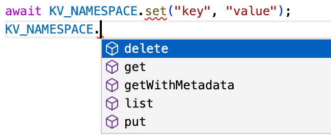
Your editor will now highlight issues and give you code completions as you type, leading to a less error-prone and more enjoyable developer experience.
Improving Workers TypeScript support: accuracy, ergonomics and interoperability
Editor highlighting incorrect use of set instead of put, and providing code completions

Improved interoperability with standard types

Cloudflare Workers implement many of the same runtime APIs as browsers, and we’re working to improve our standards compliance even more with the WinterCG. However, there will always be fundamental differences between what browsers and Workers can do. For example, browsers can play audio files, whereas Workers have direct access to Cloudflare’s network for storing globally-distributed data. This mismatch means that the runtime APIs and types provided by each platform are different, which in turn makes it difficult to use Workers types with frameworks, like Remix, that run the same files on the Cloudflare network and in the browser. These files need to be type-checked against lib.dom.d.ts, which is incompatible with our types.

To solve this problem, we now generate a separate version of our types that can be selectively imported, without having to include @cloudflare/workers-types in your tsconfig.json’s types field. Here’s an example of what this looks like:

import type { KVNamespace } from "@cloudflare/workers-types";

declare const USERS_NAMESPACE: KVNamespace;

In addition, we automatically generate a diff of our types against TypeScript’s lib.webworker.d.ts. Going forward, we’ll use this to identify areas where we can further improve our spec-compliance.

Improved compatibility with compatibility dates

Cloudflare maintains strong backwards compatibility promises for all the APIs we provide. We use compatibility flags and dates to make breaking changes in a backwards-compatible way. Sometimes these compatibility flags change the types. For example, the global_navigator flag adds a new navigator global, and the url_standard flag changes the URLSearchParams constructor signature.

We now allow you to select the version of the types that matches your compatibility date, so you can be sure you’re not using features that won’t be supported at runtime.

{
  "compilerOptions": {
    ...
    "types": ["@cloudflare/workers-types/2022-08-04"]
  }
}

Improved integration with Wrangler

In addition to compatibility dates, your Worker environment configuration also impacts the runtime and type API surface. If you have bindings such as KV namespaces or R2 buckets configured in your wrangler.toml, these need to be reflected in TypeScript types. Similarly, custom text, data and WebAssembly module rules need to be declared so TypeScript knows the types of exports. Previously, it was up to you to create a separate ambient TypeScript file containing these declarations.

To keep wrangler.toml as the single source of truth, you can now run npx wrangler types to generate this file automatically.

For example, the following wrangler.toml…

kv_namespaces = [{ binding = "MY_NAMESPACE", id = "..." }]
rules = [{ type = "Text", globs = ["**/*.txt"] }]

…generates these ambient types:

interface Env {
  MY_NAMESPACE: KVNamespace;
}
declare module "*.txt" {
  const value: string;
  export default value;
}

Improved integrated documentation and changelogs

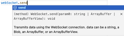
Code completions provide a great way for developers new to the Workers platform to explore the API surface. We now include the documentation for standard APIs from TypeScript’s official types in our types. We’re also starting the process of bringing docs for Cloudflare specific APIs into them too.
Improving Workers TypeScript support: accuracy, ergonomics and interoperability

For developers already using the Workers platform, it can be difficult to see how types are changing with each release of @cloudflare/workers-types. To avoid type errors and highlight new features, we now generate a detailed changelog with each release that splits out new, changed and removed definitions.

How does type generation work under the hood?

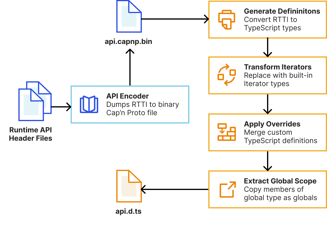
As mentioned earlier, we’ve completely rebuilt the automatic type generation scripts to be more reliable, extensible and maintainable. This means developers will get improved types as soon as new versions of the runtime are published. Our system now uses workerd’s new runtime-type-information (RTTI) system to query types of Workers runtime APIs, rather than attempting to extract this information from parsed C++ ASTs.

// Encode the KV namespace type without any compatibility flags enabled
CompatibilityFlags::Reader flags = {};
auto builder = rtti::Builder(flags);
auto type = builder.structure<KvNamespace>();
capnp::TextCodec codec;
auto encoded = codec.encode(type);
KJ_DBG(encoded); // (name = "KvNamespace", members = [ ... ], ...)

We then pass this RTTI to a TypeScript program that uses the TypeScript Compiler API to generate declarations and perform AST transformations to tidy them up. This is built into workerd’s Bazel build system, meaning generating types is now a single bazel build //types:types command. We leverage Bazel’s cache to rebuild as little as possible during generation.

import ts, { factory as f } from "typescript";

const keyParameter = f.createParameterDeclaration(
  /* decorators */ undefined,
  /* modifiers */ undefined,
  /* dotDotDotToken */ undefined,
  "key",
  /* questionToken */ undefined,
  f.createTypeReferenceNode("string")
);
const returnType = f.createTypeReferenceNode("Promise", [
  f.createUnionTypeNode([
    f.createTypeReferenceNode("string"),
    f.createLiteralTypeNode(f.createNull()),
  ]),
]);
const getMethod = f.createMethodSignature(
  /* modifiers */ undefined,
  "get",
  /* questionToken */ undefined,
  /* typeParameters */ undefined,
  [keyParameter],
  returnType
);
const kvNamespace = f.createInterfaceDeclaration(
  /* decorators */ undefined,
  /* modifiers */ undefined,
  "KVNamespace",
  /* typeParameters */ undefined,
  /* heritageClauses */ undefined,
  [getMethod]
);

const file = ts.createSourceFile("file.ts", "", ts.ScriptTarget.ESNext);
const printer = ts.createPrinter();
const output = printer.printNode(ts.EmitHint.Unspecified, kvNamespace, file);
console.log(output); // interface KVNamespace { get(key: string): Promise<string | null>; }
Improving Workers TypeScript support: accuracy, ergonomics and interoperability

Whilst the auto-generated types correctly describe the JavaScript interface of Workers runtime APIs, TypeScript provides additional features we can use to provide higher-fidelity types and improve developer ergonomics. Our system allows us to handwrite partial TypeScript “overrides” that get merged with the auto-generated types. This enables us to…

  • Add type parameters (generics) to types such as ReadableStream and avoid any typed values.
  • Specify the correspondence between input and output types with method overloads. For example, KVNamespace#get() should return a string when the type argument is text, but ArrayBuffer when it’s arrayBuffer.
  • Rename types to match TypeScript standards and reduce verbosity.
  • Fully-replace a type for more accurate declarations. For example, we replace WebSocketPair with a const declaration for better types with Object.values().
  • Provide types for values that are internally untyped such as the Request#cf object.
  • Hide internal types that aren’t usable in your workers.

Previously, these overrides were defined in separate TypeScript files to the C++ declarations they were overriding. This meant they often fell out-of-sync with the original declarations. In the new system, overrides are defined alongside the originals with C++ macros, meaning they can be reviewed alongside runtime implementation changes. See the README for workerd’s JavaScript glue code for many more details and examples.

Try typing with workers-types today!

We encourage you to upgrade to the latest version of @cloudflare/workers-types with npm install --save-dev @cloudflare/workers-types@latest, and try out the new wrangler types command. We’ll be publishing a new version of the types with each workerd release. Let us know what you think on the Cloudflare Developers Discord, and please open a GitHub issue if you find any types that could be improved.


Doubling down on local development with Workers: Miniflare meets workerd

Post Syndicated from Brendan Coll original https://blog.cloudflare.com/miniflare-and-workerd/

Doubling down on local development with Workers: Miniflare meets workerd

Doubling down on local development with Workers: Miniflare meets workerd

Local development gives you a fully-controllable and easy-to-debug testing environment. At the start of this year, we brought this experience to Workers developers by launching Miniflare 2.0: a local Cloudflare Workers simulator. Miniflare 2 came with features like step-through debugging support, detailed console.logs, pretty source-mapped error pages, live reload and a highly-configurable unit testing environment. Not only that, but we also incorporated Miniflare into Wrangler, our Workers CLI, to enable wrangler dev’s —local mode.

Today, we’re taking local development to the next level! In addition to introducing new support for migrating existing projects to your local development environment, we’re making it easier to work with your remote data—locally! Most importantly, we’re releasing a much more accurate Miniflare 3, powered by the recently open-sourced workerd runtime—the same runtime used by Cloudflare Workers!

Enabling local development with workerd

One of the superpowers of having a local development environment is that you can test changes without affecting users in production. A great local environment offers a level of fidelity on par with production.

The way we originally approached local development was with Miniflare 2, which reimplemented Workers runtime APIs in JavaScript. Unfortunately, there were subtle behavior mismatches between these re-implementations and the real Workers runtime. These types of issues are really difficult for developers to debug, as they don’t appear locally, and step-through debugging of deployed Workers isn’t possible yet. For example, the following Worker returns responses successfully in Miniflare 2, so we might assume it’s safe to publish:

let cachedResponsePromise;
export default {
  async fetch(request, env, ctx) {
    // Let's imagine this fetch takes a few seconds. To speed up our worker, we
    // decide to only fetch on the first request, and reuse the result later.
    // This works fine in Miniflare 2, so we must be good right?
    cachedResponsePromise ??= fetch("https://example.com");
    return (await cachedResponsePromise).clone();
  },
};

However, as soon as we send multiple requests to our deployed Worker, it fails with Error: Cannot perform I/O on behalf of a different request. The problem here is that response bodies created in one request’s handler cannot be accessed from a different request’s handler. This limitation allows Cloudflare to improve overall Worker performance, but it was almost impossible for Miniflare 2 to detect these types of issues locally. In this particular case, the best solution is to cache using fetch itself.

Additionally, because the Workers runtime uses a very recent version of V8, it supports some JavaScript features that aren’t available in all versions of Node.js. This meant a few features implemented in Workers, like Array#findLast, weren’t always available in Miniflare 2.

With the Workers runtime now open-sourced, Miniflare 3 can leverage the same implementations that are deployed on Cloudflare’s network, giving bug-for-bug compatibility and practically eliminating behavior mismatches. 🎉

Doubling down on local development with Workers: Miniflare meets workerd
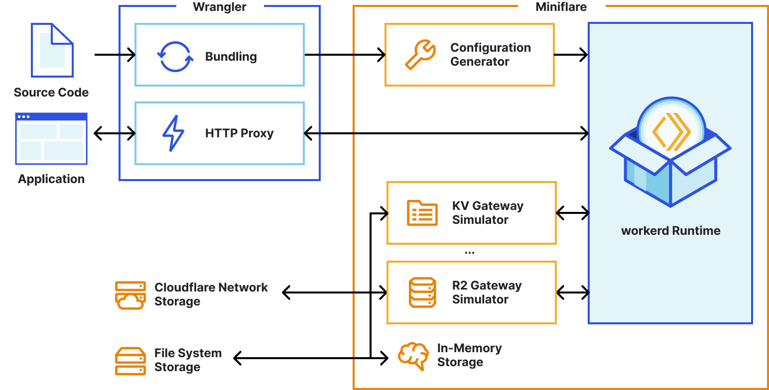
Miniflare 3’s new simplified architecture using worked

This radically simplifies our implementation too. We were able to remove over 50,000 lines of code from Miniflare 2. Of course, we still kept all the Miniflare special-sauce that makes development fun like live reload and detailed logging. 🙂

Doubling down on local development with Workers: Miniflare meets workerd

Local development with real data

We know that many developers choose to test their Workers remotely on the Cloudflare network as it gives them the ability to test against real data. Testing against fake data in staging and local environments is sometimes difficult, as it never quite matches the real thing.

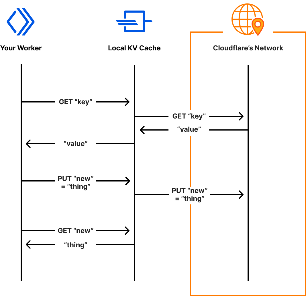
With Miniflare 3, we’re blurring the lines between local and remote development, by bringing real data to your machine as an experimental opt-in feature. If enabled, Miniflare will read and write data to namespaces on the Cloudflare network, as your Worker would when deployed. This is only supported with Workers KV for now, but we’re exploring similar solutions for R2 and D1.

Doubling down on local development with Workers: Miniflare meets workerd
Miniflare’s system for accessing real KV data, reads and writes are cached locally for future accesses

A new default for Wrangler

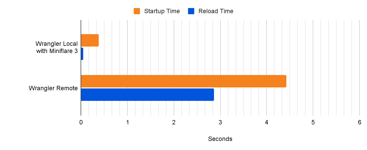
With Miniflare 3 now effectively as accurate as the real Workers environment, and the ability to access real data locally, we’re revisiting the decision to make remote development the initial Wrangler experience. In a future update, wrangler dev --local will become the default. --local will no longer be required. Benchmarking suggests this will bring an approximate 10x reduction to startup and a massive 60x reduction to script reload times! Over the next few weeks, we’ll be focusing on further optimizing Wrangler’s performance to bring you the fastest Workers development experience yet!

Doubling down on local development with Workers: Miniflare meets workerd

wrangler init --from-dash

We want all developers to be able to take advantage of the improved local experience, so we’re making it easy to start a local Wrangler project from an existing Worker that’s been developed in the Cloudflare dashboard. With Node.js installed, run npx wrangler init –from-dash <your_worker_name> in your terminal to set up a new project with all your existing code and bindings such as KV namespaces configured. You can now seamlessly continue development of your application locally, taking advantage of all the developer experience improvements Wrangler and Miniflare provide. When you’re ready to deploy your worker, run npx wrangler publish.

Looking to the future

Over the next few months, the Workers team is planning to further improve the local development experience with a specific focus on automated testing. Already, we’ve released a preliminary API for programmatic end-to-end tests with wrangler dev, but we’re also investigating ways of bringing Miniflare 2’s Jest/Vitest environments to workerd. We’re also considering creating extensions for popular IDEs to make developing workers even easier. 👀

Miniflare 3.0 is now included in Wrangler! Try it out by running npx wrangler@latest dev --experimental-local. Let us know what you think in the #wrangler channel on the Cloudflare Developers Discord, and please open a GitHub issue if you hit any unexpected behavior.

How Cloudflare instruments services using Workers Analytics Engine

Post Syndicated from Jen Sells original https://blog.cloudflare.com/using-analytics-engine-to-improve-analytics-engine/

How Cloudflare instruments services using Workers Analytics Engine

How Cloudflare instruments services using Workers Analytics Engine

Workers Analytics Engine is a new tool, announced earlier this year, that enables developers and product teams to build time series analytics about anything, with high dimensionality, high cardinality, and effortless scaling. We built Analytics Engine for teams to gain insights into their code running in Workers, provide analytics to end customers, or even build usage based billing.

In this blog post we’re going to tell you about how we use Analytics Engine to build Analytics Engine. We’ve instrumented our own Analytics Engine SQL API using Analytics Engine itself and use this data to find bugs and prioritize new product features. We hope this serves as inspiration for other teams who are looking for ways to instrument their own products and gather feedback.

Why do we need Analytics Engine?

Analytics Engine enables you to generate events (or “data points”) from Workers with just a few lines of code. Using the GraphQL or SQL API, you can query these events and create useful insights about the business or technology stack. For more about how to get started using Analytics Engine, check out our developer docs.

Since we released the Analytics Engine open beta in September, we’ve been adding new features at a rapid clip based on feedback from developers. However, we’ve had two big gaps in our visibility into the product.

First, our engineering team needs to answer classic observability questions, such as: how many requests are we getting, how many of those requests result in errors, what are the nature of these errors, etc. They need to be able to view both aggregated data (like average error rate, or p99 response time) and drill into individual events.

Second, because this is a newly launched product, we are looking for product insights. By instrumenting the SQL API, we can understand the queries our customers write, and the errors they see, which helps us prioritize missing features.

We realized that Analytics Engine would be an amazing tool for both answering our technical observability questions, and also gathering product insight. That’s because we can log an event for every query to our SQL API, and then query for both aggregated performance issues as well as individual errors and queries that our customers run.

In the next section, we’re going to walk you through how we use Analytics Engine to monitor that API.

Adding instrumentation to our SQL API

The Analytics Engine SQL API lets you query events data in the same way you would an ordinary database. For decades, SQL has been the most common language for querying data. We wanted to provide an interface that allows you to immediately start asking questions about your data without having to learn a new query language.

Our SQL API parses user SQL queries, transforms and validates them, and then executes them against backend database servers. We then write information about the query back into Analytics Engine so that we can run our own analytics.
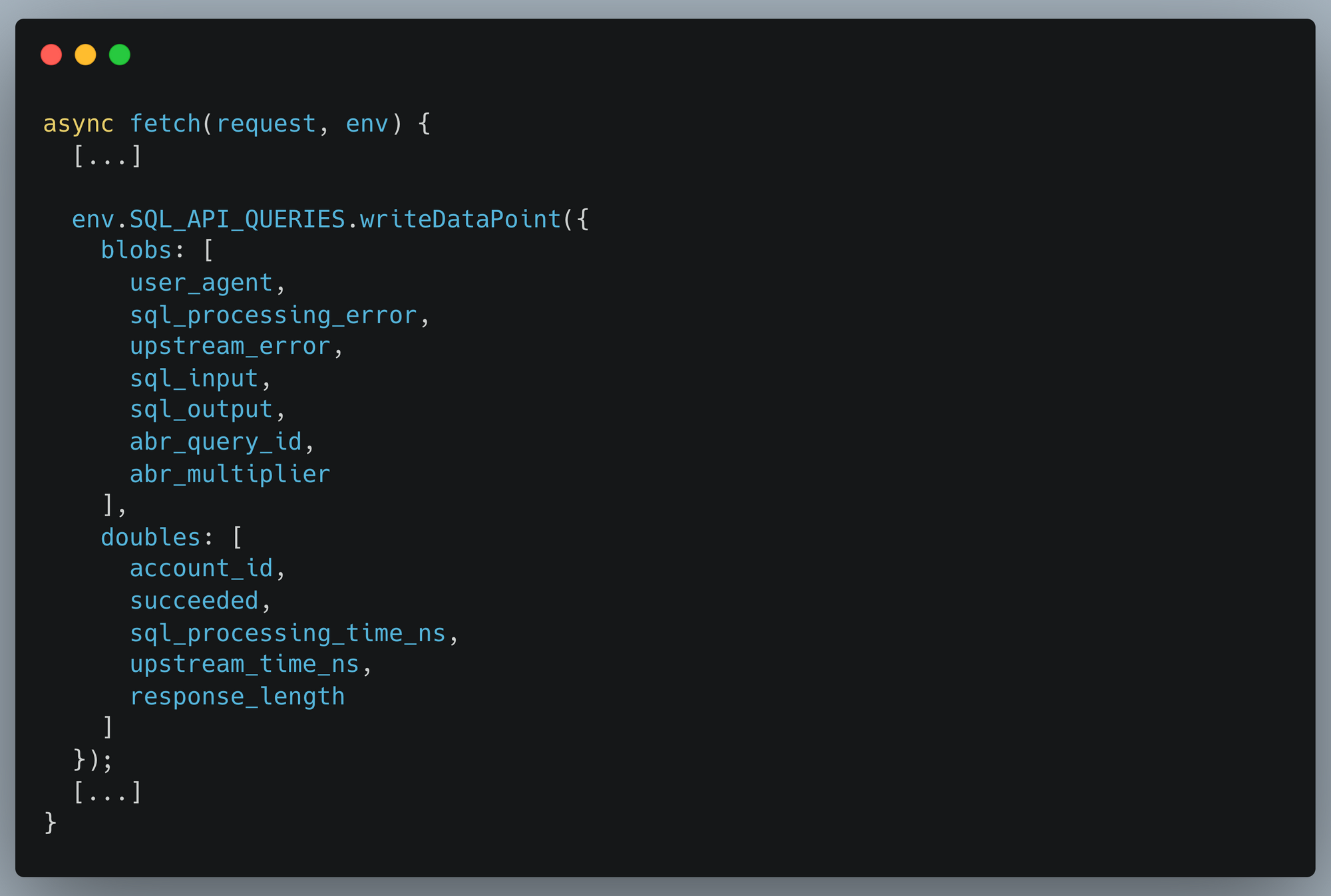
Writing data into Analytics Engine from a Cloudflare Worker is very simple and explained in our documentation. We instrument our SQL API in the same way our users do, and this code excerpt shows the data we write into Analytics Engine:

How Cloudflare instruments services using Workers Analytics Engine

With that data now being stored in Analytics Engine, we can then pull out insights about every field we’re reporting.

Querying for insights

Having our analytics in an SQL database gives you the freedom to write any query you might want. Compared to using something like metrics which are often predefined and purpose specific, you can define any custom dataset desired, and interrogate your data to ask new questions with ease.

We need to support datasets comprising trillions of data points. In order to accomplish this, we have implemented a sampling method called Adaptive Bit Rate (ABR). With ABR, if you have large amounts of data, your queries may be returned sampled events in order to respond in reasonable time. If you have more typical amounts of data, Analytics Engine will query all your data. This allows you to run any query you like and still get responses in a short length of time. Right now, you have to account for sampling in how you make your queries, but we are exploring making it automatic.

Any data visualization tool can be used to visualize your analytics. At Cloudflare, we heavily use Grafana (and you can too!). This is particularly useful for observability use cases.

Observing query response times

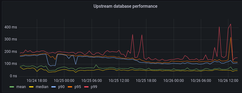
One query we pay attention to gives us information about the performance of our backend database clusters:

How Cloudflare instruments services using Workers Analytics Engine

As you can see, the 99% percentile (corresponding to the 1% most complex queries to execute) sometimes spikes up to about 300ms. But on average our backend responds to queries within 100ms.

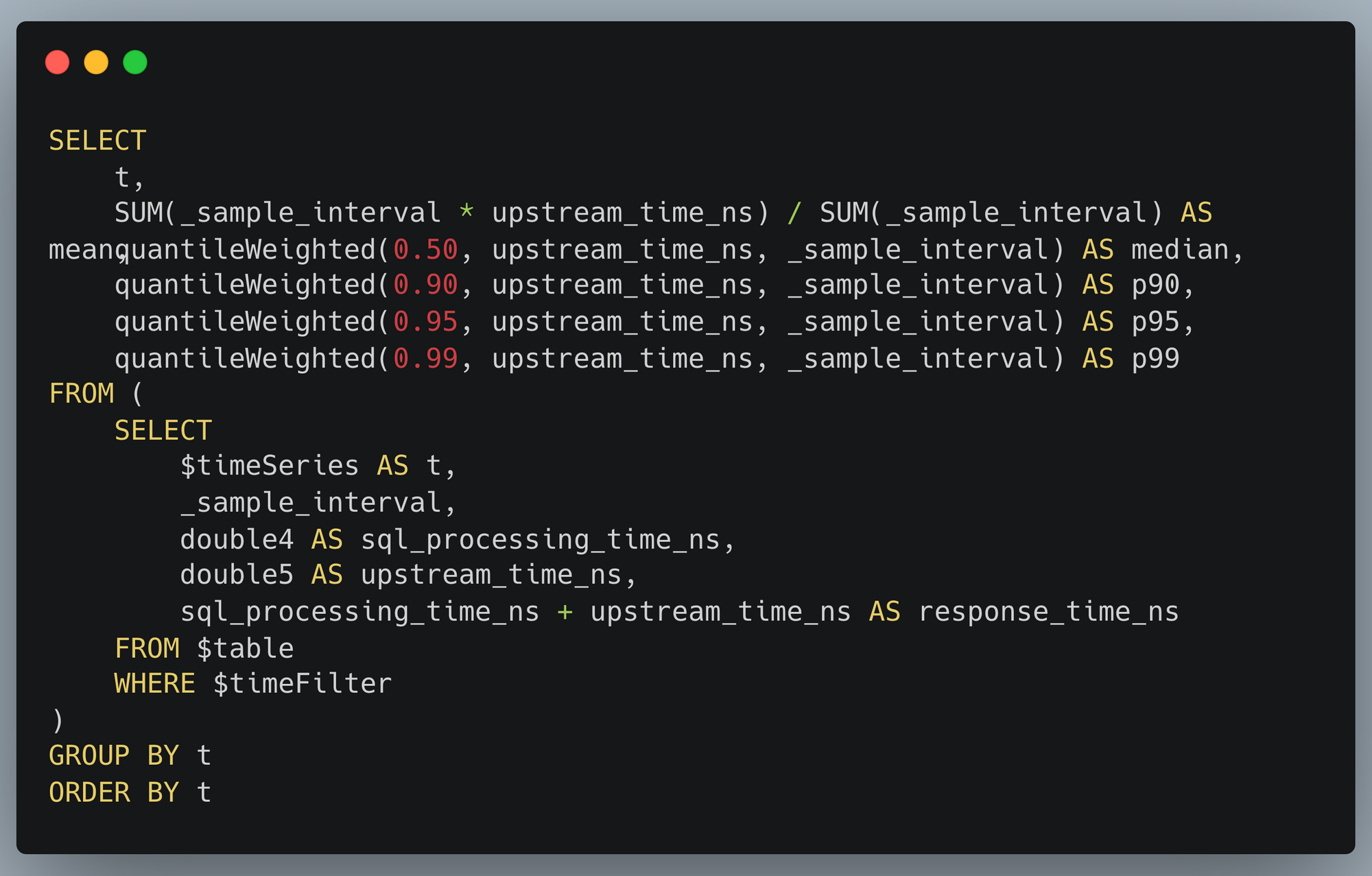
This visualization is itself generated from an SQL query:

How Cloudflare instruments services using Workers Analytics Engine

Customer insights from high-cardinality data

Another use of Analytics Engine is to draw insights out of customer behavior. Our SQL API is particularly well-suited for this, as you can take full advantage of the power of SQL. Thanks to our ABR technology, even expensive queries can be carried out against huge datasets.

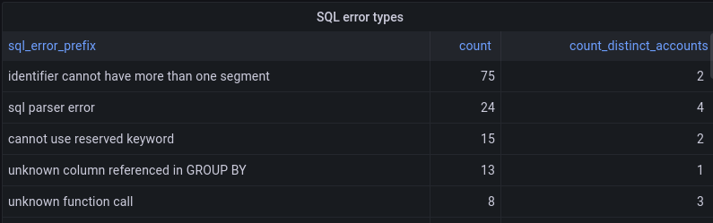
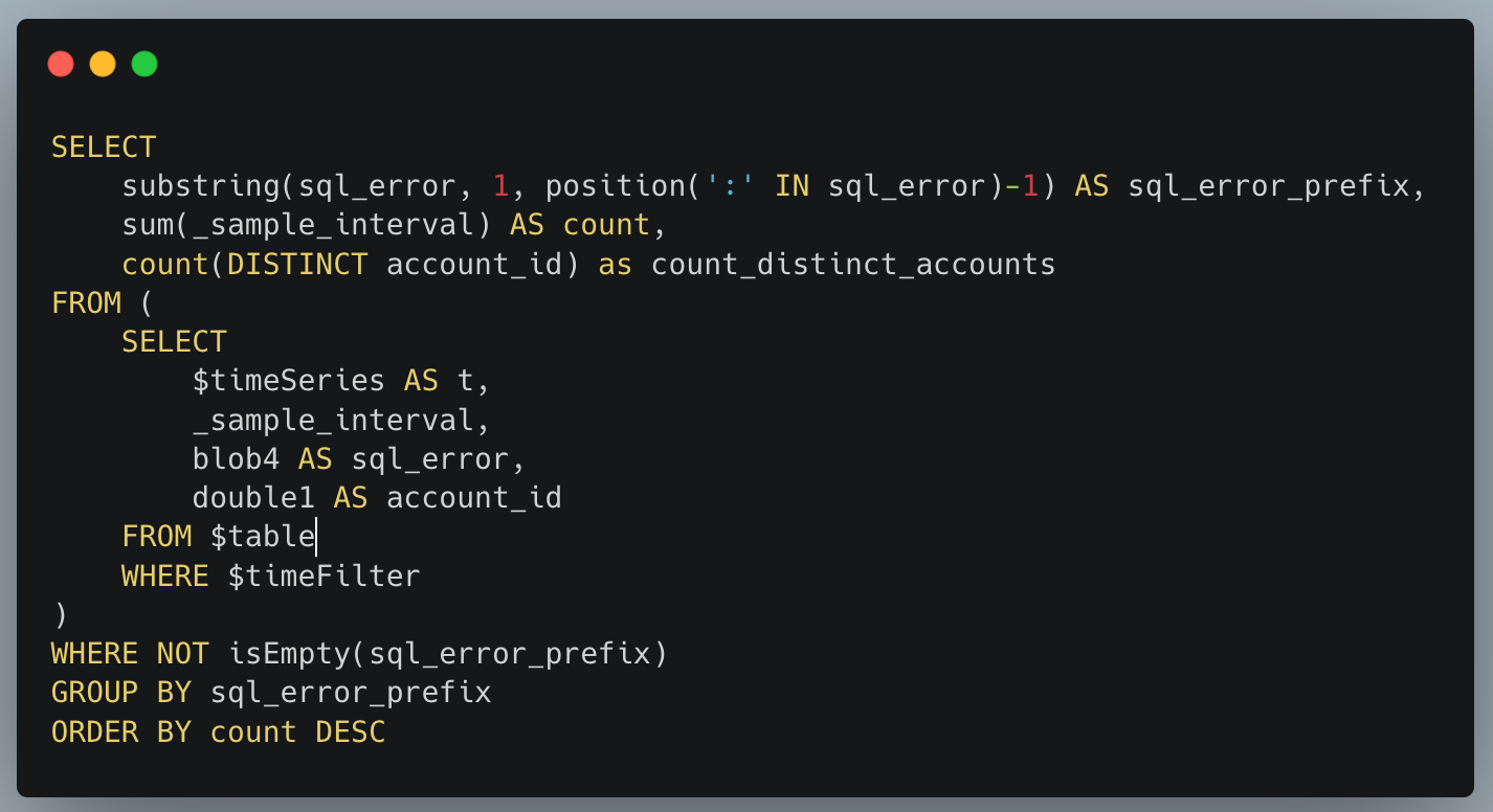
We use this ability to help prioritize improvements to Analytics Engine. Our SQL API supports a fairly standard dialect of SQL but isn’t feature-complete yet. If a user tries to do something unsupported in an SQL query, they get back a structured error message. Those error messages are reported into Analytics Engine. We’re able to aggregate the kinds of errors that our customers encounter, which helps inform which features to prioritize next.

How Cloudflare instruments services using Workers Analytics Engine

The SQL API returns errors in the format of type of error: more details, and so we can take the first portion before the colon to give us the type of error. We group by that, and get a count of how many times that error happened and how many users it affected:

How Cloudflare instruments services using Workers Analytics Engine

To perform the above query using an ordinary metrics system, we would need to represent each error type with a different metric. Reporting that many metrics from each microservice creates scalability challenges. That problem doesn’t happen with Analytics Engine, because it’s designed to handle high-cardinality data.

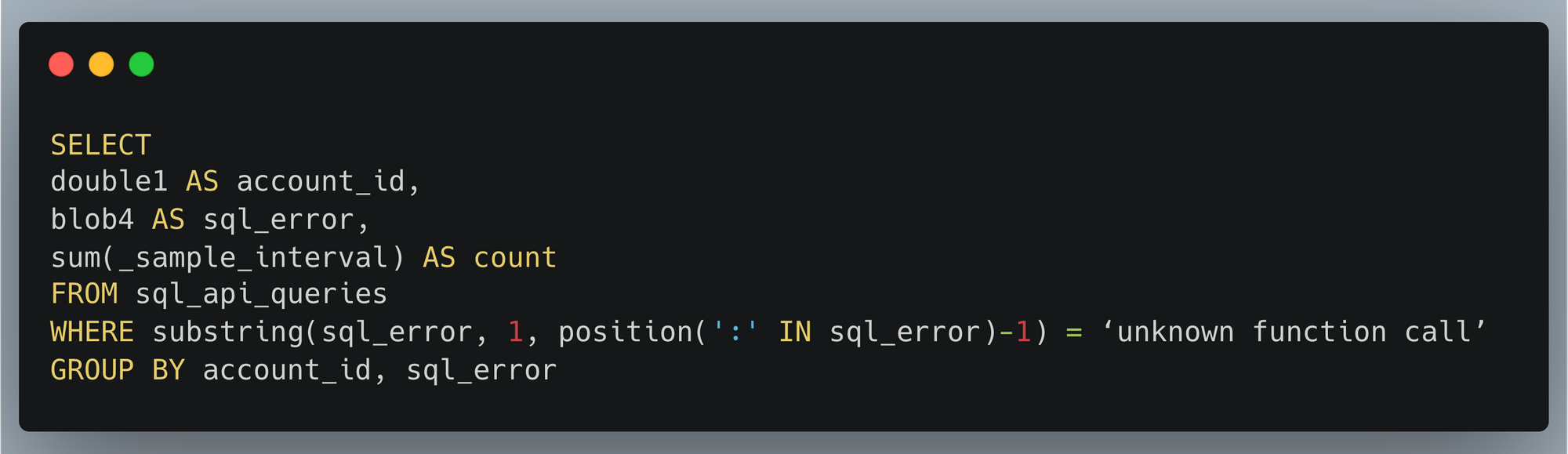
Another big advantage of a high-cardinality store like Analytics Engine is that you can dig into specifics. If there’s a large spike in SQL errors, we may want to find which customers are having a problem in order to help them or identify what function they want to use. That’s easy to do with another SQL query:

How Cloudflare instruments services using Workers Analytics Engine

Inside Cloudflare, we have historically relied on querying our backend database servers for this type of information. Analytics Engine’s SQL API now enables us to open up our technology to our customers, so they can easily gather insights about their services at any scale!

Conclusion and what’s next

The insights we gathered about usage of the SQL API are a super helpful input to our product prioritization decisions. We already added support for substring and position functions which were used in the visualizations above.

Looking at the top SQL errors, we see numerous errors related to selecting columns. These errors are mostly coming from some usability issues related to the Grafana plugin. Adding support for the DESCRIBE function should alleviate this because without this, the Grafana plugin doesn’t understand the table structure. This, as well as other improvements to our Grafana plugin, is on our roadmap.

We also can see that users are trying to query time ranges for older data that no longer exists. This suggests that our customers would appreciate having extended data retention. We’ve recently extended our retention from 31 to 92 days, and we will keep an eye on this to see if we should offer further extension.

We saw lots of errors related to common mistakes or misunderstandings of proper SQL syntax. This indicates that we could provide better examples or error explanations in our documentation to assist users with troubleshooting their queries.

Stay tuned into our developer docs to be informed as we continue to iterate and add more features!

You can start using Workers Analytics Engine Now! Analytics Engine is now in open beta with free 90-day retention. Start using it  today or join our Discord community to talk with the team.

Съдът окончателно отхвърли иск за клевета срещу Биволъ от шведски студент

Post Syndicated from Екип на Биволъ original https://bivol.bg/ziad-vks.html

петък 18 ноември 2022


Съдебен иск за клевета срешу Биволъ от шведския гражданин Зияд Тарек Ахмад е окончателно отхвърлен от Върховния касационен съд с Определение от 14 ноември 2022 г. Решението е подробно мотивирано…

For your eyes only: improving Netflix video quality with neural networks

Post Syndicated from Netflix Technology Blog original https://netflixtechblog.com/for-your-eyes-only-improving-netflix-video-quality-with-neural-networks-5b8d032da09c

by Christos G. Bampis, Li-Heng Chen and Zhi Li

When you are binge-watching the latest season of Stranger Things or Ozark, we strive to deliver the best possible video quality to your eyes. To do so, we continuously push the boundaries of streaming video quality and leverage the best video technologies. For example, we invest in next-generation, royalty-free codecs and sophisticated video encoding optimizations. Recently, we added another powerful tool to our arsenal: neural networks for video downscaling. In this tech blog, we describe how we improved Netflix video quality with neural networks, the challenges we faced and what lies ahead.

How can neural networks fit into Netflix video encoding?

There are, roughly speaking, two steps to encode a video in our pipeline:

  1. Video preprocessing, which encompasses any transformation applied to the high-quality source video prior to encoding. Video downscaling is the most pertinent example herein, which tailors our encoding to screen resolutions of different devices and optimizes picture quality under varying network conditions. With video downscaling, multiple resolutions of a source video are produced. For example, a 4K source video will be downscaled to 1080p, 720p, 540p and so on. This is typically done by a conventional resampling filter, like Lanczos.
  2. Video encoding using a conventional video codec, like AV1. Encoding drastically reduces the amount of video data that needs to be streamed to your device, by leveraging spatial and temporal redundancies that exist in a video.

We identified that we can leverage neural networks (NN) to improve Netflix video quality, by replacing conventional video downscaling with a neural network-based one. This approach, which we dub “deep downscaler,” has a few key advantages:

  • A learned approach for downscaling can improve video quality and be tailored to Netflix content.
  • It can be integrated as a drop-in solution, i.e., we do not need any other changes on the Netflix encoding side or the client device side. Millions of devices that support Netflix streaming automatically benefit from this solution.
  • A distinct, NN-based, video processing block can evolve independently, be used beyond video downscaling and be combined with different codecs.

Of course, we believe in the transformative potential of NN throughout video applications, beyond video downscaling. While conventional video codecs remain prevalent, NN-based video encoding tools are flourishing and closing the performance gap in terms of compression efficiency. The deep downscaler is our pragmatic approach to improving video quality with neural networks.

Our approach to NN-based video downscaling

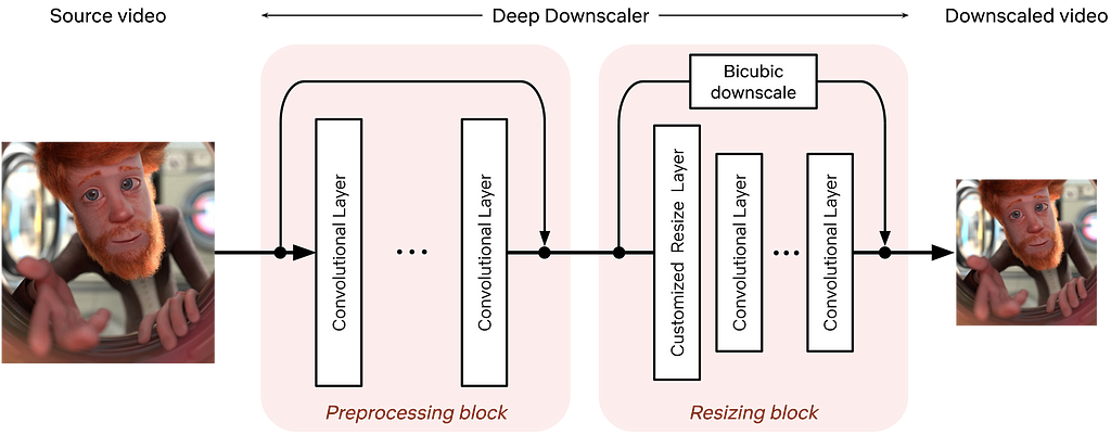
The deep downscaler is a neural network architecture designed to improve the end-to-end video quality by learning a higher-quality video downscaler. It consists of two building blocks, a preprocessing block and a resizing block. The preprocessing block aims to prefilter the video signal prior to the subsequent resizing operation. The resizing block yields the lower-resolution video signal that serves as input to an encoder. We employed an adaptive network design that is applicable to the wide variety of resolutions we use for encoding.

Architecture of the deep downscaler model, consisting of a preprocessing block followed by a resizing block.

During training, our goal is to generate the best downsampled representation such that, after upscaling, the mean squared error is minimized. Since we cannot directly optimize for a conventional video codec, which is non-differentiable, we exclude the effect of lossy compression in the loop. We focus on a robust downscaler that is trained given a conventional upscaler, like bicubic. Our training approach is intuitive and results in a downscaler that is not tied to a specific encoder or encoding implementation. Nevertheless, it requires a thorough evaluation to demonstrate its potential for broad use for Netflix encoding.

Improving Netflix video quality with neural networks

The goal of the deep downscaler is to improve the end-to-end video quality for the Netflix member. Through our experimentation, involving objective measurements and subjective visual tests, we found that the deep downscaler improves quality across various conventional video codecs and encoding configurations.

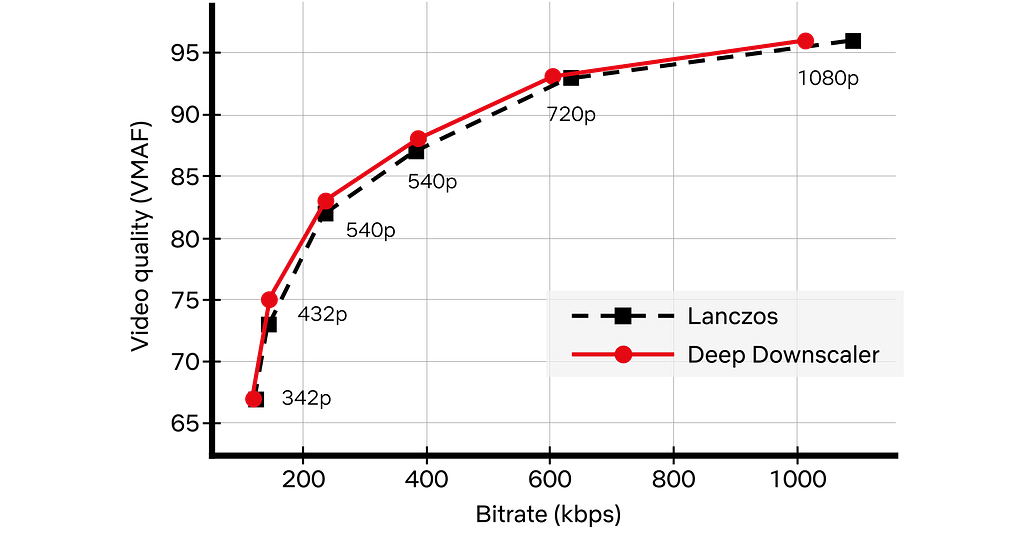
For example, for VP9 encoding and assuming a bicubic upscaler, we measured an average VMAF Bjøntegaard-Delta (BD) rate gain of ~5.4% over the traditional Lanczos downscaling. We have also measured a ~4.4% BD rate gain for VMAF-NEG. We showcase an example result from one of our Netflix titles below. The deep downscaler (red points) delivered higher VMAF at similar bitrate or yielded comparable VMAF scores at a lower bitrate.

Besides objective measurements, we also conducted human subject studies to validate the visual improvements of the deep downscaler. In our preference-based visual tests, we found that the deep downscaler was preferred by ~77% of test subjects, across a wide range of encoding recipes and upscaling algorithms. Subjects reported a better detail preservation and sharper visual look. A visual example is shown below.

Left: Lanczos downscaling; right: deep downscaler. Both videos are encoded with VP9 at the same bitrate and were upscaled to FHD resolution (1920×1080). You may need to zoom in to see the visual difference.

We also performed A/B testing to understand the overall streaming impact of the deep downscaler, and detect any device playback issues. Our A/B tests showed QoE improvements without any adverse streaming impact. This shows the benefit of deploying the deep downscaler for all devices streaming Netflix, without playback risks or quality degradation for our members.

How do we apply neural networks at scale efficiently?

Given our scale, applying neural networks can lead to a significant increase in encoding costs. In order to have a viable solution, we took several steps to improve efficiency.

  • The neural network architecture was designed to be computationally efficient and also avoid any negative visual quality impact. For example, we found that just a few neural network layers were sufficient for our needs. To reduce the input channels even further, we only apply NN-based scaling on luma and scale chroma with a standard Lanczos filter.
  • We implemented the deep downscaler as an FFmpeg-based filter that runs together with other video transformations, like pixel format conversions. Our filter can run on both CPU and GPU. On a CPU, we leveraged oneDnn to further reduce latency.

Integrating neural networks into our next-generation encoding platform

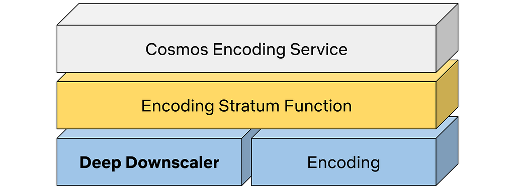
The Encoding Technologies and Media Cloud Engineering teams at Netflix have jointly innovated to bring Cosmos, our next-generation encoding platform, to life. Our deep downscaler effort was an excellent opportunity to showcase how Cosmos can drive future media innovation at Netflix. The following diagram shows a top-down view of how the deep downscaler was integrated within a Cosmos encoding microservice.

A top-down view of integrating the deep downscaler into Cosmos.

A Cosmos encoding microservice can serve multiple encoding workflows. For example, a service can be called to perform complexity analysis for a high-quality input video, or generate encodes meant for the actual Netflix streaming. Within a service, a Stratum function is a serverless layer dedicated to running stateless and computationally-intensive functions. Within a Stratum function invocation, our deep downscaler is applied prior to encoding. Fueled by Cosmos, we can leverage the underlying Titus infrastructure and run the deep downscaler on all our multi-CPU/GPU environments at scale.

What lies ahead

The deep downscaler paves the path for more NN applications for video encoding at Netflix. But our journey is not finished yet and we strive to improve and innovate. For example, we are studying a few other use cases, such as video denoising. We are also looking at more efficient solutions to applying neural networks at scale. We are interested in how NN-based tools can shine as part of next-generation codecs. At the end of the day, we are passionate about using new technologies to improve Netflix video quality. For your eyes only!

Acknowledgments

We would like to acknowledge the following individuals for their help with the deep downscaler project:

Lishan Zhu, Liwei Guo, Aditya Mavlankar, Kyle Swanson and Anush Moorthy (Video Image and Encoding team), Mariana Afonso and Lukas Krasula (Video Codecs and Quality team), Ameya Vasani (Media Cloud Engineering team), Prudhvi Kumar Chaganti (Streaming Encoding Pipeline team), Chris Pham and Andy Rhines (Data Science and Engineering team), Amer Ather (Netflix performance team), the Netflix Metaflow team and Prof. Alan Bovik (University of Texas at Austin).


For your eyes only: improving Netflix video quality with neural networks was originally published in Netflix TechBlog on Medium, where people are continuing the conversation by highlighting and responding to this story.

AWS Security Profile: Reef D’Souza, Principal Solutions Architect

Post Syndicated from Maddie Bacon original https://aws.amazon.com/blogs/security/aws-security-profile-reef-dsouza-principal-solutions-architect/

In the weeks leading up to AWS re:invent 2022, I’ll share conversations I’ve had with some of the humans who work in AWS Security who will be presenting at the conference, and get a sneak peek at their work and sessions. In this profile, I interviewed Reef D’Souza, Principal Solutions Architect.

How long have you been at AWS and what do you do in your current role?

I’ve been at AWS for about six and a half years. During my time here, I’ve worked in AWS Professional Services as a security consultant in New York and Los Angeles. I worked with customers in Financial Services, Healthcare, Telco, and Media & Entertainment to build security controls that align with the AWS Cloud Adoption Framework Security Epics (now Security Perspective) so that these customers could run highly regulated workloads on AWS. In the last two years, I’ve switched to a dual role of being a Solution Architect for Independent Software Vendors (ISVs) and Digital Native Businesses (DNBs) in Canada while helping them with their security and privacy.

How did you get started in security?

I started out trying to make it as a software developer but realized I enjoy breaking things apart with my skepticism of security claims. While I was getting my master’s degree in Information Systems, I started to specialize in applying machine learning (ML) to anomaly detection systems and then went on to application security vulnerability management and testing while working at different security startups in New York. My customers were mostly in financial services, looking to threat model their apps, prioritize their risks, and take action.

How do you explain your job to non-technical friends and family?

I tell them that I work with companies who tell me what they’re worried about, which includes stolen credit card data or healthcare data, and then help those customers put technology in place to prevent or detect a security event. This often goes down the path of comparing me to the television show Mr. Robot or fictional espionage scenarios. When I say I work for Amazon, I often get asked whether I can track packages down for Thanksgiving and the holiday season.

What are you currently working on that you’re excited about?

I’ve been diving deep into the world of privacy engineering. As an SA for software companies in Canada, many of whom want to launch in Europe and other parts of the world that have strict privacy regulations, it’s a frequent topic. However, privacy discussions are often steeped in legal-speak. My customers’ technical stakeholders say that it all sounds like English but doesn’t make any sense. So my goal is to help them understand privacy risks and translate these risks to mechanisms that can be implemented in customers’ workloads. The last cool thing I worked on with AWS Privacy specialists on the ProServe SAS team was a workshop for AWS re:Inforce 2022 this past July.

You’re presenting at re:Invent this year. Can you give us a sneak peek of your session?

My session is Securing serverless workloads on AWS. It’s a chalk talk that walks the attendee through the shared responsibility model for serverless applications built with AWS Lambda. We then dive deeper into how to threat model for security risks and use AWS services to secure the application and test for vulnerabilities in the CI/CD pipeline. I cover classic risks like the OWASP Top 10 and how customers must think about verifying trusted third-party libraries with AWS CodeArtifact, deploying trusted code by using AWS Signer, and identifying vulnerabilities in their code with Amazon CodeGuru.

What do you hope attendees take away from your session?

Customers with vulnerability management programs must grasp a paradigm shift that there are no servers to scan anymore. Here is where the lines are blurred between traditional vulnerability management and application security. I hope attendees of my sessions leave with a better understanding of their responsibilities in terms of risks and where AWS services can help them build secure applications and do so earlier in the development lifecycle.

What’s your favorite Amazon Leadership Principle and why?

Insist on the Highest Standards. Shoddy craftsmanship based on planning for short-term wins, inefficiency, and wasteful spending are massive pet peeves of mine. This principle ties so closely with Customer Obsession, because the quality of our work impacts the long-term trust that others place in us. When there is an issue, it motivates us to find the root cause and shows up in our focus on operational excellence.

What’s the best career advice you’ve ever received?

After I got out of graduate school, I entered the world thinking I knew everything. My first manager gave me the advice to keep asking questions, though. Knowing things doesn’t necessarily mean that your knowledge applies to a problem. You have to think beyond just a technical solution. When I joined Amazon, this felt natural as part of our Working Backwards process.

What’s the thing you’re most proud of in your career?

I worked on a COVID contact-tracing data lake project in the early stages of the pandemic. With some of the best security and data engineers on the team, we were able to threat model for the various components of the analytics environment, which housed data subject to HIPAA, the California Consumer Privacy Act (CCPA), the E.U. General Data Protection Regulation (GDPR) and many other healthcare and general privacy regulations. We released a working analytics solution within five or so months after March 2020. At the time, building these types of environments usually took over a year.

If you had to pick an industry outside of security, what would you want to do?

Motorcycle travel writing. It combines my favorite activities of meeting new people, learning new languages and cultures, trying new cuisines (cooking and eating), and sharing the experience with others.

 
If you have feedback about this post, submit comments in the Comments section below. If you have questions about this post, contact AWS Support.

Want more AWS Security news? Follow us on Twitter.

Author

Maddie Bacon

Maddie (she/her) is a technical writer for Amazon Security with a passion for creating meaningful content that focuses on the human side of security and encourages a security-first mindset. She previously worked as a reporter and editor, and has a BA in Mathematics. In her spare time, she enjoys reading, traveling, and staunchly defending the Oxford comma.

Reef D’Souza

Reef D’Souza

Reef is a Principal Solutions Architect focused on secrets management, privacy, threat modeling and web application security for companies across financial services, healthcare, media & entertainment and technology vendors.

AWS AppSync GraphQL APIs Supports JavaScript Resolvers

Post Syndicated from Marcia Villalba original https://aws.amazon.com/blogs/aws/aws-appsync-graphql-apis-supports-javascript-resolvers/

Starting today, AWS AppSync supports JavaScript resolvers and provides a resolver evaluation engine to test them before publishing them to the cloud.

AWS AppSync, launched in 2017, is a service that allows you to build, manage, and host GraphQL APIs in the cloud. AWS AppSync connects your GraphQL schema to different data sources using resolvers. Resolvers are how AWS AppSync translates GraphQL requests and fetches information from the different data sources.

Until today, many customers had to write their resolvers using Apache Velocity Template Language (VTL). To write VTL resolvers, many developers needed to learn a new language, and that discouraged them from taking advantage of the capabilities that resolvers offer. And when they did write them, developers faced the challenge of how to test the VTL resolvers. That is why many customers resorted to writing their complex resolvers as AWS Lambda functions and then creating a simple VTL resolver that invoked that function. This adds more complexity to their applications, as now they have to maintain and operate this new Lambda function.

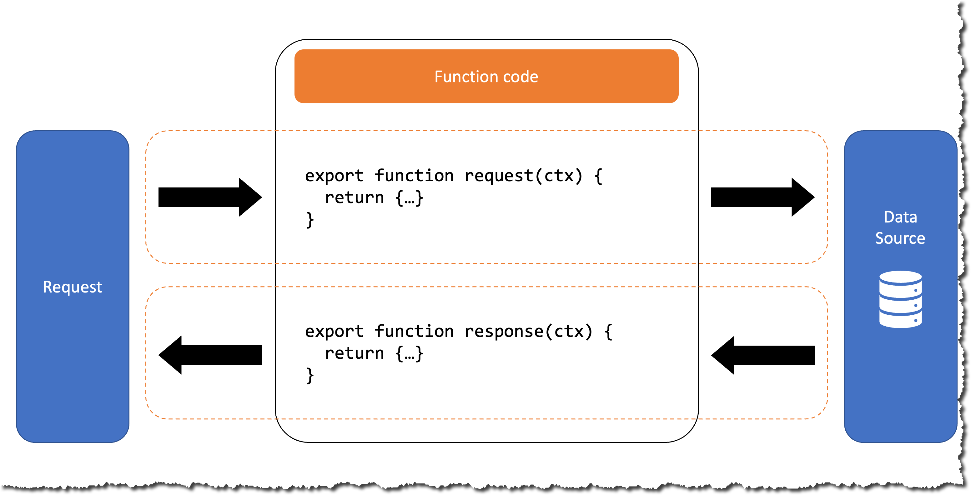
AWS AppSync executes resolvers on a GraphQL field. Sometimes, applications require executing multiple operations to resolve a single GraphQL field. When using AWS AppSync, developers can create pipeline resolvers to compose operations (called functions) and execute them in sequence. Each function performs an operation over a data source, for example, fetching an item from an Amazon DynamoDB table.

How a function works

Introducing AWS AppSync JavaScript pipeline resolvers
Now, in addition to VTL, developers can use JavaScript to write their functions. You can mix functions written in JavaScript and VTL inside a pipeline resolver.

This new launch comes with two new NPM libraries to simplify development: @aws-appsync/eslint-plugin to catch and fix problems quickly during development and @aws-appsync/utils to provide type validation and autocompletion in code editors.

Developers can test their JavaScript code using AWS AppSync’s new API command, evaluate-code. During a test, the code is validated for correctness and evaluated with mock data. This helps developers validate their code before pushing their changes to the cloud.

With this launch, AWS AppSync becomes one of the easiest ways for your applications to talk to almost any AWS service. You can write an HTTP function that calls any AWS service with an API endpoint using JavaScript and use that function as part of your pipeline. For example, you can create a pipeline resolver that is invoked when a query on a GraphQL field occurs. This field returns the translated text in Spanish of an item stored in a table. This pipeline resolver is composed of two functions, one that fetches data from a DynamoDB table and one that uses Amazon Translate API to translate the item text into Spanish.

function awsTranslateRequest(Text, SourceLanguageCode, SourceLanguageCode) {
  return {
    method: 'POST',
    resourcePath: '/',
    params: {
      headers: {
        'content-type': 'application/x-amz-json-1.1',
        'x-amz-target': 'AWSShineFrontendService_20170701.TranslateText',
      },
      body: JSON.stringify({ Text, SourceLanguageCode, SourceLanguageCode }),
    },
  };
}

Getting started
You can create JavaScript functions from the AWS AppSync console or using the AWS Command Line Interface (CLI). Let’s create a pipeline resolver that gets an item from an existing DynamoDB table using the AWS CLI. This resolver only has one function.

When creating a new AWS AppSync function, you need to provide the code for that function. Create a new JavaScript file and copy the following code snippet.

import { util } from '@aws-appsync/utils';

/**
 * Request a single item from the attached DynamoDB table
 * @param ctx the request context
 */
export function request(ctx) {
  return {
    operation: 'GetItem',
    key: util.dynamodb.toMapValues({ id: ctx.args.id }),
  };
}

/**
 * Returns the DynamoDB result directly
 * @param ctx the request context
 */
export function response(ctx) {
  return ctx.result;
}

All functions need to have a request and response method, and in each of these methods, you can perform the operations for fulfilling the business need.

To get started, first make sure that you have the latest version of the AWS CLI, that you have a DynamoDB table created, and that you have an AWS AppSync API. Then you can create the function in AWS AppSync using the AWS CLI create-function command and the file you just created. This command returns the function ID. To create the resolver, pass the function ID, the GraphQL operation, and the field where you want to apply the resolver. In the documentation, you can find a detailed tutorial on how to create pipeline resolvers.

Testing a resolver
To test a function, use the evaluate-code command from AWS CLI or AWS SDK. This command calls the AWS AppSync service and evaluates the code with the provided context. To automate the test, you can use any JavaScript testing and assertion library. For example, the following code snippet uses Jest to validate the returned results programmatically.

import * as AWS from 'aws-sdk'
import { readFile } from 'fs/promises'
const appsync = new AWS.AppSync({ region: 'us-east-2' })
const file = './functions/updateItem.js'

test('validate an update request', async () => {
  const context = JSON.stringify({
    arguments: {
      input: { id: '<my-id>', title: 'change!', description: null },
    },
  })
  const code = await readFile(file, { encoding: 'utf8' })
  const runtime = { name: 'APPSYNC_JS', runtimeVersion: '1.0.0' }
  const params = { context, code, runtime, function: 'request' }

  const response = await appsync.evaluateCode(params).promise()
  expect(response.error).toBeUndefined()
  expect(response.evaluationResult).toBeDefined()
  const result = JSON.parse(response.evaluationResult)
  expect(result.key.id.S).toEqual(context.arguments.input.id)
  expect(result.update.expressionNames).not.toHaveProperty('#id')
  expect(result.update.expressionNames).toHaveProperty('#title')
  expect(result.update.expressionNames).toHaveProperty('#description')
  expect(result.update.expressionValues).not.toHaveProperty(':description')
})

In this way, you can add your API tests to your build process and validate that you coded the resolvers correctly before you push the changes to the cloud.

Get started today
The support for JavaScript AWS AppSync resolvers in AWS AppSync is available for all Regions that currently support AWS AppSync. You can start using this feature today from the AWS Management Console, AWS CLI, or Amazon CloudFormation.

Learn more about this launch by visiting the AWS AppSync service page.

— Marcia

Announcing the AWS Well-Architected Data Analytics Lens

Post Syndicated from Dhiraj Thakur original https://aws.amazon.com/blogs/big-data/announcing-the-aws-well-architected-data-analytics-lens/

We are delighted to announce the release of the Data Analytics Lens. The lens consists of a lens whitepaper and an AWS-created lens available in the Lens Catalog of the AWS Well-Architected Tool. The AWS Well-Architected Framework provides a consistent approach to evaluate architectures and implement scalable designs. With the AWS Well-Architected Framework, cloud architects, system architects, engineers, and developers can build secure, high-performance, resilient, and efficient infrastructure for their applications and workloads.

Using the Lens in the Tool’s Lens Catalog, you can directly assess your Analytics workload in the console, and produce a set of actionable results for customized improvement plans recommended by the Tool.

The updated Data Analytics Lens outlines the most up-to-date steps for performing an AWS Well-Architected review that empowers you to assess and identify technical risks of your data analytics platforms. The new whitepaper and Lens cover multiple analytics use cases and scenarios, and provide comprehensive guidance to help you design your analytics applications in accordance with AWS best practices.

The new Data Analytics Lens offers implementation guidance you can use to deliver secure, high performance and reliable workloads, all with an eye toward maintaining cost-effectiveness and sustainability.

For more information on AWS Well-Architected Lenses, refer to AWS Well-Architected.

What’s new in the Data Analytics Lens?

The Data Analytics Lens is a collection of customer-proven design principles, best practices, and prescriptive guidance to help you adopt a cloud-centered approach to running analytics on AWS. These recommendations are based on insights that AWS has gathered from customers, AWS Partners, the field, and our own analytics technical specialist communities.

This version covers the following topics:

  • New Lens for the Well-Architected Tool in the Lens Catalog
  • New Data Mesh analytics user scenario
  • Included guidance on building ACID compliant data lakes using Iceberg
  • Included guidance on adding business context to your data catalog to improve searchability and access
  • How best to leverage Serverless to build sustainable data pipelines
  • Expanded advanced performance tuning techniques
  • Additional content for analytics scenario use cases
  • Links to updated blogs and product documentation, partner solutions, training content, and how-to videos

The lens highlights some of the most common areas for assessment and improvement. It’s designed to align with and provide insights across the six pillars of the AWS Well-Architected Framework:

  • Operational excellence – Includes the ability to support development and run workloads effectively, gain insight into your operations, and continually improve supporting processes and procedures to deliver business value.
  • Security – Includes the ability to protect data, systems, and assets to take advantage of cloud technologies to improve your security.
  • Reliability – Includes the ability of a system to automatically recover from infrastructure or service disruptions, dynamically acquire computing resources to meet demand, and mitigate disruptions such as misconfiguration or transient network issues.
  • Performance efficiency – Includes the efficient use of computing resources to meet requirements and the maintenance of that efficiency as demand changes and technologies evolve.
  • Cost optimization – Includes the continual process of system refinement and improvement over the entire lifecycle to optimize cost, from the initial design of your first proof of concept to the ongoing operation of production workloads.
  • Sustainability – Includes minimizing the environmental impacts of running cloud workloads. Topics including benchmarking, trading data accuracy for carbon, encouraging a data minimization culture, implementing data retention processes, optimizing data modeling, preventing unnecessary data movement, and efficiently managing analytics infrastructure.

The new Data Analytics Lens provides guidance that can help you make appropriate design decisions in line with your business requirements. By applying the techniques detailed in this lens to your architecture, you can validate the resiliency and efficiency of your design. This lens also provides recommendations to address any gaps you may identify.

Who should use the Data Analytics Lens?

The Data Analytics Lens is intended for all AWS customers who use analytics processes to run their workloads.

We believe that the lens will be valuable regardless of your stage of cloud adoption: whether you’re launching your first analytics workloads on AWS, migrating existing services to the cloud, or working to extend and improve existing AWS analytics workloads.

The material is intended to support customers in roles such as architects, developers, and operations team members.

Conclusion

Applying the Data Analytics Lens to your existing architectures can validate the stability and efficiency of your design and provide recommendations to address identified gaps.

For more information about building your own Well-Architected systems using the Data Analytics Lens, see the Data Analytics Lens whitepaper. For information about on the new Lens, please see the Well Architected Tool and Lens Catalog briefs. If you require additional expert guidance, contact your AWS account team to engage a Specialist Solutions Architect.

To learn more about supported analytics solutions, customer case studies, and additional resources, refer to Architecture Best Practices for Analytics & Big Data.


About the authors

Russell Jackson is a Senior Solutions Architect at AWS based in the UK. Russell has over 15 years of analytics experience and is passionate about Big Data, event driven-architectures and building environmentally sustainable data pipelines. Outside of work, Russell enjoys road cycling, wild swimming and traveling.

Theo Tolv is a Senior Analytics Architect based in Stockholm, Sweden. He’s worked with small and big data for most of his career, and has built applications running on AWS since 2008. In his spare time he likes to tinker with electronics and read space opera.

Bruce Ross is a Senior Solutions Architect at AWS in the New York Area. Bruce is the Lens Leader for the Well-Architected Framework. He has been involved in IT and Content Development for over 20 years. He is an avid sailor and angler, and enjoys R&B, jazz, and classical music.


Dhiraj Thakur is a Solutions Architect with Amazon Web Services. He works with AWS customers and partners to provide guidance on enterprise cloud adoption, migration, and strategy. He is passionate about technology and enjoys building and experimenting in the analytics and AI/ML space.

Pragnesh Shah is a Solutions Architect in the Partner Organisation. He is specialist in migration, modernisation, Cloud strategy, designing and delivering data and analytics capabilities. Outside of work, he spends time with family and nature. He likes to record nature sound and practice Zen meditation.

Introducing attribute-based access controls (ABAC) for Amazon SQS

Post Syndicated from James Beswick original https://aws.amazon.com/blogs/compute/introducing-attribute-based-access-controls-abac-for-amazon-sqs/

This post is written by Vikas Panghal (Principal Product Manager), and Hardik Vasa (Senior Solutions Architect).

Amazon Simple Queue Service (SQS) is a fully managed message queuing service that makes it easier to decouple and scale microservices, distributed systems, and serverless applications. SQS queues enable asynchronous communication between different application components and ensure that each of these components can keep functioning independently without losing data.

Today we’re announcing support for attribute-based access control (ABAC) using queue tags with the SQS service. As an AWS customer, if you use multiple SQS queues to achieve better application decoupling, it is often challenging to manage access to individual queues. In such cases, using tags can enable you to classify these resources in different ways, such as by owner, category, or environment.

This blog post demonstrates how to use tags to allow conditional access to SQS queues. You can use attribute-based access control (ABAC) policies to grant access rights to users through policies that combine attributes together. ABAC can be helpful in rapidly growing environments, where policy management for each individual resource can become cumbersome.

ABAC for SQS is supported in all Regions where SQS is currently available.

Overview

SQS supports tagging of queues. Each tag is a label comprising a customer-defined key and an optional value that can make it easier to manage, search for, and filter resources. Tags allows you to assign metadata to your SQS resources. This can help you track and manage the costs associated with your queues, provide enhanced security in your AWS Identity and Access Management (IAM) policies, and lets you easily filter through thousands of queues.

SQS queue options in the console

The preceding image shows SQS queue in AWS Management Console with two tags – ‘auto-delete’ with value of ‘no’ and ‘environment’ with value of ‘prod’.

Attribute-based access controls (ABAC) is an authorization strategy that defines permissions based on tags attached to users and AWS resources. With ABAC, you can use tags to configure IAM access permissions and policies for your queues. ABAC hence enables you to scale your permissions management easily. You can author a single permissions policy in IAM using tags that you create per business role, and you no longer need to update the policy while adding each new resource.

You can also attach tags to AWS Identity and Access Management (IAM) principals to create an ABAC policy. These ABAC policies can be designed to allow SQS operations when the tag on the IAM user or role making the call matches the SQS queue tag.

ABAC provides granular and flexible access control based on attributes and values, reduces security risk because of misconfigured role-based policy, and easily centralizes auditing and access policy management.

ABAC enables two key use cases:

  1. Tag-based Access Control: You can use tags to control access to your SQS queues, including control plane and data plane API calls.
  2. Tag-on-Create: You can enforce tags during the creation of SQS queues and deny the creation of SQS resources without tags.

Tagging for access control

Let’s take a look at a couple of examples on using tags for access control.

Let’s say that you would want to restrict IAM user to all SQS actions for all queues that include a resource tag with the key environment and the value production. The following IAM policy helps to fulfill the requirement.

{
    "Version": "2012-10-17",
    "Statement": [
        {
            "Sid": "DenyAccessForProd",
            "Effect": "Deny",
            "Action": "sqs:*",
            "Resource": "*",
            "Condition": {
                "StringEquals": {
                    "aws:ResourceTag/environment": "prod"
                }
            }
        }
    ]
}

Now, for instance you need to restrict IAM policy for any operation on resources with a given tag with key environment and value production as an argument within the API call, the following IAM policy helps fulfill the requirements.

{
    "Version": "2012-10-17",
    "Statement": [
        {
            "Sid": "DenyAccessForStageProduction",
            "Effect": "Deny",
            "Action": "sqs:*",
            "Resource": "*",
            "Condition": {
                "StringEquals": {
                    "aws:RequestTag/environment": "production"
                }
            }
        }
    ]
}

Creating IAM user and SQS queue using AWS Management Console

Configuration of the ABAC on SQS resources is a two-step process. The first step is to tag your SQS resources with tags. You can use the AWS API, the AWS CLI, or the AWS Management Console to tag your resources. Once you have tagged the resources, create an IAM policy that allows or denies access to SQS resources based on their tags.

This post reviews the step-by-step process of creating ABAC policies for controlling access to SQS queues.

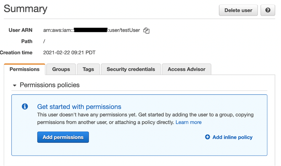
Create an IAM user

  1. Navigate to the AWS IAM console and choose User from the left navigation pane.
  2. Choose Add Users and provide a name in the User name text box.
  3. Check the Access key – Programmatic access box and choose Next:Permissions.
  4. Choose Next:Tags.
  5. Add tag key as environment and tag value as beta
  6. Select Next:Review and then choose Create user
  7. Copy the access key ID and secret access key and store in a secure location.

IAM configuration

Add IAM user permissions

  1. Select the IAM user you created.
  2. Choose Add inline policy.
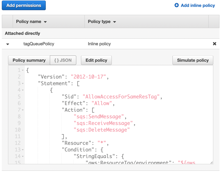
  3. In the JSON tab, paste the following policy:
    {
        "Version": "2012-10-17",
        "Statement": [
            {
                "Sid": "AllowAccessForSameResTag",
                "Effect": "Allow",
                "Action": [
                    "sqs:SendMessage",
                    "sqs:ReceiveMessage",
                    "sqs:DeleteMessage"
                ],
                "Resource": "*",
                "Condition": {
                    "StringEquals": {
                        "aws:ResourceTag/environment": "${aws:PrincipalTag/environment}"
                    }
                }
            },
            {
                "Sid": "AllowAccessForSameReqTag",
                "Effect": "Allow",
                "Action": [
                    "sqs:CreateQueue",
                    "sqs:DeleteQueue",
                    "sqs:SetQueueAttributes",
                    "sqs:tagqueue"
                ],
                "Resource": "*",
                "Condition": {
                    "StringEquals": {
                        "aws:RequestTag/environment": "${aws:PrincipalTag/environment}"
                    }
                }
            },
            {
                "Sid": "DenyAccessForProd",
                "Effect": "Deny",
                "Action": "sqs:*",
                "Resource": "*",
                "Condition": {
                    "StringEquals": {
                        "aws:ResourceTag/stage": "prod"
                    }
                }
            }
        ]
    }
    
  4. Choose Review policy.
  5. Choose Create policy.
    Create policy

The preceding permissions policy ensures that the IAM user can call SQS APIs only if the value of the request tag within the API call matches the value of the environment tag on the IAM principal. It also makes sure that the resource tag applied to the SQS queue matches the IAM tag applied on the user.

Creating IAM user and SQS queue using AWS CloudFormation

Here is the sample CloudFormation template to create an IAM user with an inline policy attached and an SQS queue.

AWSTemplateFormatVersion: "2010-09-09"
Description: "CloudFormation template to create IAM user with custom in-line policy"
Resources:
    IAMPolicy:
        Type: "AWS::IAM::Policy"
        Properties:
            PolicyDocument: |
                {
                    "Version": "2012-10-17",
                    "Statement": [
                        {
                            "Sid": "AllowAccessForSameResTag",
                            "Effect": "Allow",
                            "Action": [
                                "sqs:SendMessage",
                                "sqs:ReceiveMessage",
                                "sqs:DeleteMessage"
                            ],
                            "Resource": "*",
                            "Condition": {
                                "StringEquals": {
                                    "aws:ResourceTag/environment": "${aws:PrincipalTag/environment}"
                                }
                            }
                        },
                        {
                            "Sid": "AllowAccessForSameReqTag",
                            "Effect": "Allow",
                            "Action": [
                                "sqs:CreateQueue",
                                "sqs:DeleteQueue",
                                "sqs:SetQueueAttributes",
                                "sqs:tagqueue"
                            ],
                            "Resource": "*",
                            "Condition": {
                                "StringEquals": {
                                    "aws:RequestTag/environment": "${aws:PrincipalTag/environment}"
                                }
                            }
                        },
                        {
                            "Sid": "DenyAccessForProd",
                            "Effect": "Deny",
                            "Action": "sqs:*",
                            "Resource": "*",
                            "Condition": {
                                "StringEquals": {
                                    "aws:ResourceTag/stage": "prod"
                                }
                            }
                        }
                    ]
                }
                
            Users: 
              - "testUser"
            PolicyName: tagQueuePolicy

    IAMUser:
        Type: "AWS::IAM::User"
        Properties:
            Path: "/"
            UserName: "testUser"
            Tags: 
              - 
                Key: "environment"
                Value: "beta"

Testing tag-based access control

Create queue with tag key as environment and tag value as prod

We will use AWS CLI to demonstrate the permission model. If you do not have AWS CLI, you can download and configure it for your machine.

Run this AWS CLI command to create the queue:

aws sqs create-queue --queue-name prodQueue —region us-east-1 —tags "environment=prod"

You receive an AccessDenied error from the SQS endpoint:

An error occurred (AccessDenied) when calling the CreateQueue operation: Access to the resource <queueUrl> is denied.

This is because the tag value on the IAM user does not match the tag passed in the CreateQueue API call. Remember that we applied a tag to the IAM user with key as ‘environment’ and value as ‘beta’.

Create queue with tag key as environment and tag value as beta

aws sqs create-queue --queue-name betaQueue —region us-east-1 —tags "environment=beta"

You see a response similar to the following, which shows the successful creation of the queue.

{
"QueueUrl": "<queueUrl>“
}

Sending message to the queue

aws sqs send-message --queue-url <queueUrl> —message-body testMessage

You will get a successful response from the SQS endpoint. The response will include MD5OfMessageBody and MessageId of the message.

{
"MD5OfMessageBody": "<MD5OfMessageBody>",
"MessageId": "<MessageId>"
}

The response shows successful message delivery to the SQS queue since the IAM user permission allows sending message with queue with tag ‘beta’.

Benefits of attribute-based access controls

The following are benefits of using attribute-based access controls (ABAC) in Amazon SQS:

  • ABAC for SQS requires fewer permissions policies – You do not have to create different policies for different job functions. You can use the resource and request tags that apply to more than one queue. This reduces the operational overhead.
  • Using ABAC, teams can scale quickly – Permissions for new resources are automatically granted based on tags when resources are appropriately tagged upon creation.
  • Use permissions on the IAM principal to restrict resource access – You can create tags for the IAM principal and restrict access to specific action only if it matches the tag on the IAM principal. This helps automate granting of request permissions.
  • Track who is accessing resources – Easily determine the identity of a session by looking at the user attributes in AWS CloudTrail to track user activity in AWS.

Conclusion

In this post, we have seen how Attribute-based access control (ABAC) policies allow you to grant access rights to users through IAM policies based on tags defined on the SQS queues.

ABAC for SQS supports all SQS API actions. Managing the access permissions via tags can save you engineering time creating complex access permissions as your applications and resources grow. With the flexibility of using multiple resource tags in the security policies, the data and compliance teams can now easily set more granular access permissions based on resource attributes.

For additional details on pricing, see Amazon SQS pricing. For additional details on programmatic access to the SQS data protection, see Actions in the Amazon SQS API Reference. For more information on SQS security, see the SQS security public documentation page. To get started with the attribute-based access control for SQS, navigate to the SQS console.

For more serverless learning resources, visit Serverless Land.

Holiday Gift Guide 2022

Post Syndicated from original https://www.backblaze.com/blog/holiday-gift-guide-2022/

The holidays: They start earlier every single year. Two weeks before Halloween, I started seeing gingerbread houses at the store. And you know someone really waited until the last minute to buy Halloween candy when they’re giving out candy canes. Gift giving is not my love language (I’m more of a quality time person), so finding the right things for my friends and family for the holidays fills me with a certain sense of angst. Luckily for me, I’m able to outsource some of the “what’s cool” contemplation to my coworkers, and you get to benefit! So without further ado, let’s get into the annual Backblaze Holiday Gift Guide for 2022 as proposed by a smorgasbord of Backblazers.

Tech and Gadgets

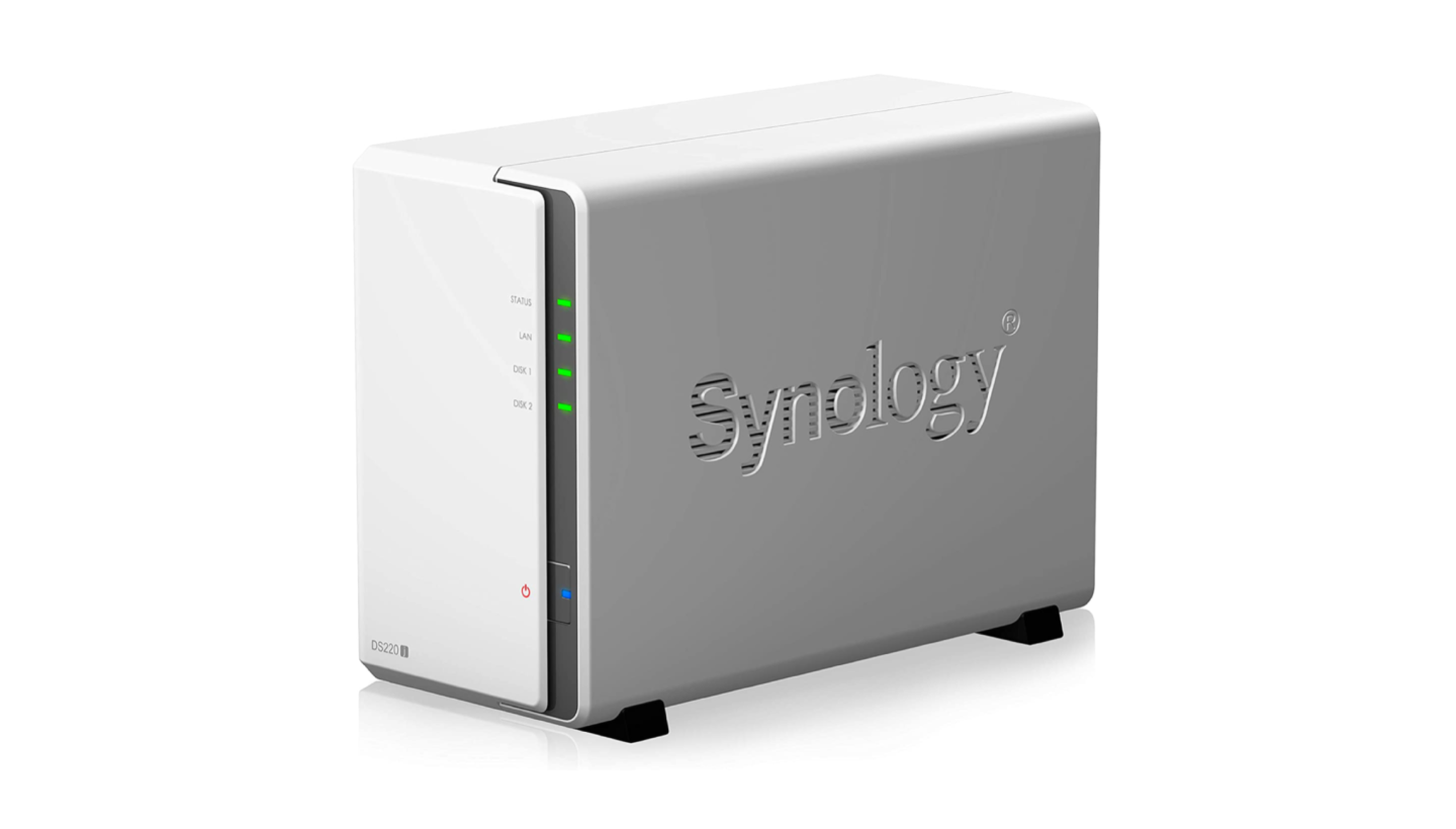
Synology NAS

Data. You know it. You love it. You have it. If you want a local device to help with your 3-2-1 backup strategy, this entry-level Synology NAS device is a great bet.

Insta 360 X3

Wide-angle and 360-degree videos are all the rage right now. If you have a shutterbug in your life, this is a great gift so they have something in their pocket, ready to capture the next viral video. After all, the best camera is the one you have with you.

Bose SoundLink Speaker

For the audiophile in your life that wants to throw a houseparty without having to set up a bunch of speaker wires, this speaker will fill the room and keep you groovin’. Or, for quieter types, it delivers your favorite murder podcast with sharp clarity.

Alfred

This app for the macOS helps you take control of your Mac and boosts your efficiency by allowing you to set up custom actions, text expansion, and hotkeys.

Valve Steam Deck

For the gamer who has everything, this is a mini computer you can travel with. It plays all of your Steam games, and it’s a great portable way to get through your backlog of games you’ve bought on sale and never had a chance to play. Although we know you’ll (or they’ll) just play Vampire Survivors the whole time.

Remarkable 2

Note taking. Has it been solved? The Remarkable 2 takes a run at making your notes and meetings easier to remember. This digital notepad is an easy way to take notes and sync them across devices.

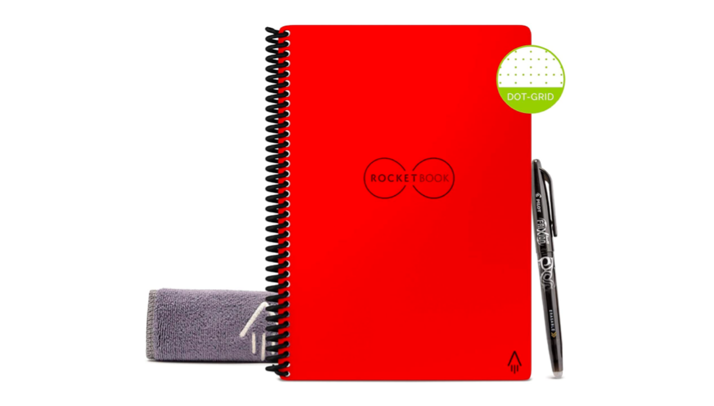
Rocketbook

Another solution for note taking: The Rocketbook (we recommend red) allows you to use a washable pen on special paper, so you can take notes, scan them, send them to the location of your choosing, and then erase the page to start over.

Ember Mug (in red, obviously)

Everyone’s favorite, an Ember mug. This keeps your drinks warm, and most importantly, if you get the red one, (we recommend red, of course) you’ll be helping global pandemic relief!

Toys and Fun Stuff

The Office Lego Set

In case you don’t get enough of the office while at the office, you can make an office in your home office, and this one will have all your favorite pals from The Office! My home office is my kitchen table, but turning it into a Lego workshop is a much better use of space.

Woobles

What better gift to give than the gift of knowledge…of crocheting? I have purchased this and am in the middle of learning to crochet. It’s fun and more importantly, adorable.

The Ted Lasso Game

We believe in believe too, Ted! The Ted Lasso party game is a fun gift in that you can open it right up and start playing. This game is full of positive vibes, just like the show. Help your players be their best selves, and maybe learn a bit about your friends and family along the way.

Blipblox

Do you have or know someone that has a little DJ brewing at their house? This Blipblox is a music exploration tool for kids as young as three years old. Help them learn all about music and get some more synth into your life!

Flying Orb Ball Toys

This tiny orb ball spins and gently glides towards a target. That makes it easy to catch and a great way to build up hand-eye coordination.

Stuff You Can Wear

Birkenstocks

What do you get the person who has everything? Another pair of Birkenstocks. With winter approaching, sandals may not be top of mind, but these are part of the standard spring and summer kit that we see around our San Mateo office.

Allbirds

Sandals not your thing? How about shoes that you can snuggle and hug? These Allbirds are part of the fluff collection, made with fluffy wool. You’ll love ’em!

Bart Bridge Patch

A patch for every occasion, and location. You probably live somewhere, and that place probably has a patch made by Bart Bridge. Show some local pride, or gift your friends a hat with a patch of that one place where that one thing happened which you will never forget, but will also never discuss.

Food and Drink

Panettone

Some say that the way to a person’s heart is through their tummy. The Panettone comes highly recommended by tummies everywhere, and just look at all those seeds! The best part about this gift is that when you hand it over, you can make a strong case about opening it and sharing.

Smoked Fish

If you have not heard of Goldbelly, it’s a great way to order food from your favorite restaurants, no matter where they are. Want to impress your holiday guests? Get this whitefish and salmon salad platter from Zucker’s in New York.

Coffee Beans

Everyone loves a good stocking stuffer, and one that we don’t think gets enough credit is getting a nice bag of coffee beans. This coffee comes highly recommended and, best of all, it’s available on Amazon for your grinding, brewing, and sipping pleasure.

Fellowship Foundry Pewter Mug

For the nerdy folks in your life, a pewter drinking mug. If you’re sitting around a Dungeons & Dragons table, you want to make sure that you’re drinking the part.

Give the Gift of Backblaze

And of course, help your friends and family back up their data with Backblaze Computer Backup. They’ll thank you for helping make sure they never lose a file again.

Happy Gift-Giving From Backblaze

I hope this gift guide helped spark some creative ideas for the upcoming gift-giving season. Comment below and tell me what gifts you’ll be looking to pick up for your friends and loved ones this year (we won’t tell them). And stay tuned for a forthcoming Backblaze Book Guide—we had so many book submissions this year, we decided to start the first annual Bookblaze Roundup.

The post Holiday Gift Guide 2022 appeared first on Backblaze Blog | Cloud Storage & Cloud Backup.

Better Cloud Security Shouldn’t Require Bigger Budgets

Post Syndicated from Aaron Wells original https://blog.rapid7.com/2022/11/17/better-cloud-security-shouldnt-require-bigger-budgets/

Stretching what you’re given

Better Cloud Security Shouldn’t Require Bigger Budgets

How can you do more when you’re constantly being given the same or less? When security budgets don’t match the pace of the cloud operations they’re tasked with securing, the only thing to do is become an expert in the stretch. It’s hard, and you might currently be under increasing stress to pull it all off.

While total overall budgets will indeed decrease, Gartner recently forecast that spending on cybersecurity and risk management would increase by 11.3% in 2023, driven in large part by a shift to cloud platforms. And what was a big factor in the increase in cloud adoption? You guessed it: the switch to remote or hybrid work models during the height of pandemic mitigation measures. These days you might have more to back up your argument for an increase in funding.

In the 2020 scramble to keep people safe by urging them to both stay home and stay employed, workforces quickly became virtual, more distributed, and incredibly reliant on cloud platforms to enable connectivity to each other. Businesses that might have dipped their toes in pre-pandemic are now taking the full cloud plunge post-pandemic.

The promise of the cloud is an interesting point to discuss. It can be cheaper to scale into the cloud, but depending on how it’s done and in what industry, it might actually require a bigger piece of the budget. But it can still be empowering and flexible. In other words, budgets will most likely keep increasing for cloud adoption. With all that said, if you’re still having trouble acquiring more budget for security, what should you do?

Finding the right fit

We’re not talking about a doomsday scenario where you’ll never see another increase in your budget. Cybersecurity and cloud security are top-of-mind topics for companies and nations around the world. However, solutions have evolved to address security organizations’ budgetary concerns. And there are reputable providers who have created offerings that can do more without asking more of your budget. This more-with-less scenario has the potential to satisfy across the board by helping you to:

  • Focus on use cases – What kind of cloud security do you need? Needlessly spending money on solutions you don’t need is tantamount to criminal behavior in the current global economic crisis. Make sure you know exactly what you need to protect, how far your perimeters extend, and the general types of available security (CSPM, CWPP, etc.). InsightCloudSec from Rapid7 is a unified platform that incorporates multiple use cases and types of cloud security.  
  • Extrapolate potential costs and prove security’s worth – Once you know what you need and the type(s) of solutions that can address it, it’s a good idea to partner with whomever controls your security budgets. Because it’s less about the costs or subscription fees you see today and more about extrapolating cost savings as cloud environments, data transfer, storage, and other aspects of that adoption grow. Then you’ll know how much or little you’ll need to engage in budget-stretching heroics.
  • Pinpoint under-one-umbrella solutions – Do you want to deal with one vendor or multiple? In the latter scenario, keep in mind the multiple support teams you’ll juggle as well as the different platforms on which those solutions will operate. There is no one-size-fits-all solution, but there are vendors that can provide a suite of broad-range capabilities so you have one point of contact and can better operationalize your cloud security.

About that whole “proving security’s worth” thing…

In this day and age, you really shouldn’t have to prove your organization’s worth. But you most likely feel that way every time you have to fight for a bigger piece of the budgetary pie. Sure, you can engage in stretching heroics, but should you have to engage in those heroics day in and day out, for years on end? Hopefully not now, when ransomware is still all the rage and nation-state-sponsored attacks are becoming more legitimate business in many parts of the world.  

Timing is everything, however, and now – at the end of the year – would be the time to pull off some of those heroics and make your case for more budget. This will enable your exploration into a solution that can do more for less. InsightCloudSec from Rapid7 is a cloud risk and compliance management platform that enables organizations to securely accelerate cloud adoption with continuous security and compliance throughout the entire software development lifecycle (SDLC).

It provides a comprehensive solution to manage and mitigate risk across even the most complex cloud environments. The platform detects risk signals in real-time and in complete context, allowing your teams to focus on the issues that present the most risk to your business based on potential impact and likelihood of exploitation.

And speaking of making things easier

Whatever your ultimate cloud security needs are, you can now learn more about tactics to help you make your case for more – or any – cloud security at your company. Plus, get a handy checklist to use when looking into a potential solution. Get started now with the 2022 edition of The Complete Cloud Security Buyer’s Guide from Rapid7. You can also read the previous entry in this blog series here.

Share and publish your Snowflake data to AWS Data Exchange using Amazon Redshift data sharing

Post Syndicated from Raks Khare original https://aws.amazon.com/blogs/big-data/share-and-publish-your-snowflake-data-to-aws-data-exchange-using-amazon-redshift-data-sharing/

Amazon Redshift is a fully managed, petabyte-scale data warehouse service in the cloud. You can start with just a few hundred gigabytes of data and scale to a petabyte or more. Today, tens of thousands of AWS customers—from Fortune 500 companies, startups, and everything in between—use Amazon Redshift to run mission-critical business intelligence (BI) dashboards, analyze real-time streaming data, and run predictive analytics. With the constant increase in generated data, Amazon Redshift customers continue to achieve successes in delivering better service to their end-users, improving their products, and running an efficient and effective business.

In this post, we discuss a customer who is currently using Snowflake to store analytics data. The customer needs to offer this data to clients who are using Amazon Redshift via AWS Data Exchange, the world’s most comprehensive service for third-party datasets. We explain in detail how to implement a fully integrated process that will automatically ingest data from Snowflake into Amazon Redshift and offer it to clients via AWS Data Exchange.

Overview of the solution

The solution consists of four high-level steps:

  1. Configure Snowflake to push the changed data for identified tables into an Amazon Simple Storage Service (Amazon S3) bucket.
  2. Use a custom-built Redshift Auto Loader to load this Amazon S3 landed data to Amazon Redshift.
  3. Merge the data from the change data capture (CDC) S3 staging tables to Amazon Redshift tables.
  4. Use Amazon Redshift data sharing to license the data to customers via AWS Data Exchange as a public or private offering.

The following diagram illustrates this workflow.

Solution Architecture Diagram

Prerequisites

To get started, you need the following prerequisites:

Configure Snowflake to track the changed data and unload it to Amazon S3

In Snowflake, identify the tables that you need to replicate to Amazon Redshift. For the purpose of this demo, we use the data in the TPCH_SF1 schema’s Customer, LineItem, and Orders tables of the SNOWFLAKE_SAMPLE_DATA database, which comes out of the box with your Snowflake account.

  1. Make sure that the Snowflake external stage name unload_to_s3 created in the prerequisites is pointing to the S3 prefix s3-redshift-loader-sourcecreated in the previous step.
  2. Create a new schema BLOG_DEMO in the DEMO_DB database:CREATE SCHEMA demo_db.blog_demo;
  3. Duplicate the Customer, LineItem, and Orders tables in the TPCH_SF1 schema to the BLOG_DEMO schema:
    CREATE TABLE CUSTOMER AS 
    SELECT * FROM snowflake_sample_data.tpch_sf1.CUSTOMER;
    CREATE TABLE ORDERS AS
    SELECT * FROM snowflake_sample_data.tpch_sf1.ORDERS;
    CREATE TABLE LINEITEM AS 
    SELECT * FROM snowflake_sample_data.tpch_sf1.LINEITEM;

  4. Verify that the tables have been duplicated successfully:
    SELECT table_catalog, table_schema, table_name, row_count, bytes
    FROM INFORMATION_SCHEMA.TABLES
    WHERE TABLE_SCHEMA = 'BLOG_DEMO'
    ORDER BY ROW_COUNT;

    unload-step-4

  5. Create table streams to track data manipulation language (DML) changes made to the tables, including inserts, updates, and deletes:
    CREATE OR REPLACE STREAM CUSTOMER_CHECK ON TABLE CUSTOMER;
    CREATE OR REPLACE STREAM ORDERS_CHECK ON TABLE ORDERS;
    CREATE OR REPLACE STREAM LINEITEM_CHECK ON TABLE LINEITEM;

  6. Perform DML changes to the tables (for this post, we run UPDATE on all tables and MERGE on the customer table):
    UPDATE customer 
    SET c_comment = 'Sample comment for blog demo' 
    WHERE c_custkey between 0 and 10; 
    UPDATE orders 
    SET o_comment = 'Sample comment for blog demo' 
    WHERE o_orderkey between 1800001 and 1800010; 
    UPDATE lineitem 
    SET l_comment = 'Sample comment for blog demo' 
    WHERE l_orderkey between 3600001 and 3600010;
    MERGE INTO customer c 
    USING 
    ( 
    SELECT n_nationkey 
    FROM snowflake_sample_data.tpch_sf1.nation s 
    WHERE n_name = 'UNITED STATES') n 
    ON n.n_nationkey = c.c_nationkey 
    WHEN MATCHED THEN UPDATE SET c.c_comment = 'This is US based customer1';

  7. Validate that the stream tables have recorded all changes:
    SELECT * FROM CUSTOMER_CHECK; 
    SELECT * FROM ORDERS_CHECK; 
    SELECT * FROM LINEITEM_CHECK;

    For example, we can query the following customer key value to verify how the events were recorded for the MERGE statement on the customer table:

    SELECT * FROM CUSTOMER_CHECK where c_custkey = 60027;

    We can see the METADATA$ISUPDATE column as TRUE, and we see DELETE followed by INSERT in the METADATA$ACTION column.
    unload-val-step-7

  8. Run the COPY command to offload the CDC from the stream tables to the S3 bucket using the external stage name unload_to_s3.In the following code, we’re also copying the data to S3 folders ending with _stg to ensure that when Redshift Auto Loader automatically creates these tables in Amazon Redshift, they get created and marked as staging tables:
    COPY INTO @unload_to_s3/customer_stg/
    FROM (select *, sysdate() as LAST_UPDATED_TS from demo_db.blog_demo.customer_check)
    FILE_FORMAT = (TYPE = PARQUET)
    OVERWRITE = TRUE HEADER = TRUE;

    COPY INTO @unload_to_s3/customer_stg/
    FROM (select *, sysdate() as LAST_UPDATED_TS from demo_db.blog_demo.customer_check)
    FILE_FORMAT = (TYPE = PARQUET)
    OVERWRITE = TRUE HEADER = TRUE;

    COPY INTO @unload_to_s3/lineitem_stg/ 
    FROM (select *, sysdate() as LAST_UPDATED_TS from demo_db.blog_demo.lineitem_check) 
    FILE_FORMAT = (TYPE = PARQUET) 
    OVERWRITE = TRUE HEADER = TRUE;

  9. Verify the data in the S3 bucket. There will be three sub-folders created in the s3-redshift-loader-source folder of the S3 bucket, and each will have .parquet data files.unload-step-9-valunload-step-9-valYou can also automate the preceding COPY commands using tasks, which can be scheduled to run at a set frequency for automatic copy of CDC data from Snowflake to Amazon S3.
  10. Use the ACCOUNTADMIN role to assign the EXECUTE TASK privilege. In this scenario, we’re assigning the privileges to the SYSADMIN role:
    USE ROLE accountadmin;
    GRANT EXECUTE TASK, EXECUTE MANAGED TASK ON ACCOUNT TO ROLE sysadmin;

  11. Use the SYSADMIN role to create three separate tasks to run three COPY commands every 5 minutes: USE ROLE sysadmin;
    /* Task to offload Customer CDC table */ 
    CREATE TASK sf_rs_customer_cdc 
    WAREHOUSE = SMALL 
    SCHEDULE = 'USING CRON 5 * * * * UTC' 
    AS 
    COPY INTO @unload_to_s3/customer_stg/ 
    FROM (select *, sysdate() as LAST_UPDATED_TS from demo_db.blog_demo.customer_check) 
    FILE_FORMAT = (TYPE = PARQUET) 
    OVERWRITE = TRUE 
    HEADER = TRUE;
    /*Task to offload Orders CDC table */ 
    CREATE TASK sf_rs_orders_cdc 
    WAREHOUSE = SMALL 
    SCHEDULE = 'USING CRON 5 * * * * UTC' 
    AS 
    COPY INTO @unload_to_s3/orders_stg/ 
    FROM (select *, sysdate() as LAST_UPDATED_TS from demo_db.blog_demo.orders_check)
    FILE_FORMAT = (TYPE = PARQUET)
    OVERWRITE = TRUE HEADER = TRUE;

    /* Task to offload Lineitem CDC table */ 
    CREATE TASK sf_rs_lineitem_cdc 
    WAREHOUSE = SMALL 
    SCHEDULE = 'USING CRON 5 * * * * UTC' 
    AS 
    COPY INTO @unload_to_s3/lineitem_stg/ 
    FROM (select *, sysdate() as LAST_UPDATED_TS from demo_db.blog_demo.lineitem_check)
    FILE_FORMAT = (TYPE = PARQUET)
    OVERWRITE = TRUE HEADER = TRUE;

    When the tasks are first created, they’re in a SUSPENDED state.

  12. Alter the three tasks and set them to RESUME state:
    ALTER TASK sf_rs_customer_cdc RESUME;
    ALTER TASK sf_rs_orders_cdc RESUME;
    ALTER TASK sf_rs_lineitem_cdc RESUME;

  13. Validate that all three tasks have been resumed successfully: SHOW TASKS;unload-setp-13-valNow the tasks will run every 5 minutes and look for new data in the stream tables to offload to Amazon S3.As soon as data is migrated from Snowflake to Amazon S3, Redshift Auto Loader automatically infers the schema and instantly creates corresponding tables in Amazon Redshift. Then, by default, it starts loading data from Amazon S3 to Amazon Redshift every 5 minutes. You can also change the default setting of 5 minutes.
  14. On the Amazon Redshift console, launch the query editor v2 and connect to your Amazon Redshift cluster.
  15. Browse to the dev database, public schema, and expand Tables.
    You can see three staging tables created with the same name as the corresponding folders in Amazon S3.
  16. Validate the data in one of the tables by running the following query:SELECT * FROM "dev"."public"."customer_stg";unload-step-16-val

Configure the Redshift Auto Loader utility

The Redshift Auto Loader makes data ingestion to Amazon Redshift significantly easier because it automatically loads data files from Amazon S3 to Amazon Redshift. The files are mapped to the respective tables by simply dropping files into preconfigured locations on Amazon S3. For more details about the architecture and internal workflow, refer to the GitHub repo.

We use an AWS CloudFormation template to set up Redshift Auto Loader. Complete the following steps:

  1. Launch the CloudFormation template.
  2. Choose Next.
    autoloader-step-2
  3. For Stack name, enter a name.
  4. Provide the parameters listed in the following table.

    CloudFormation Template Parameter Allowed Values Description
    RedshiftClusterIdentifier Amazon Redshift cluster identifier Enter the Amazon Redshift cluster identifier.
    DatabaseUserName Database user name in the Amazon Redshift cluster The Amazon Redshift database user name that has access to run the SQL script.
    DatabaseName S3 bucket name The name of the Amazon Redshift primary database where the SQL script is run.
    DatabaseSchemaName Database name in Amazon Redshift The Amazon Redshift schema name where the tables are created.
    RedshiftIAMRoleARN Default or the valid IAM role ARN attached to the Amazon Redshift cluster The IAM role ARN associated with the Amazon Redshift cluster. Your default IAM role is set for the cluster and has access to your S3 bucket, leave it at the default.
    CopyCommandOptions Copy option; default is delimiter ‘|’ gzip

    Provide the additional COPY command data format parameters.

    If InitiateSchemaDetection = Yes, then the process attempts to detect the schema and automatically set the suitable copy command options.

    In the event of failure on schema detection or when InitiateSchemaDetection = No, then this value is used as the default COPY command options to load data.

    SourceS3Bucket S3 bucket name The S3 bucket where the data is stored. Make sure the IAM role that is associated to the Amazon Redshift cluster has access to this bucket.
    InitiateSchemaDetection Yes/No

    Set to Yes to dynamically detect the schema prior to file load and create a table in Amazon Redshift if it doesn’t exist already. If a table already exists, then it won’t drop or recreate the table in Amazon Redshift.

    If schema detection fails, the process uses the default COPY options as specified in CopyCommandOptions.

    The Redshift Auto Loader uses the COPY command to load data into Amazon Redshift. For this post, set CopyCommandOptions as follows, and configure any supported COPY command options:

    delimiter '|' dateformat 'auto' TIMEFORMAT 'auto'

    autoloader-input-parameters

  5. Choose Next.
  6. Accept the default values on the next page and choose Next.
  7. Select the acknowledgement check box and choose Create stack.
    autoloader-step-7
  8. Monitor the progress of the Stack creation and wait until it is complete.
  9. To verify the Redshift Auto Loader configuration, sign in to the Amazon S3 console and navigate to the S3 bucket you provided.
    You should see a new directory s3-redshift-loader-source is created.
    autoloader-step-9

Copy all the data files exported from Snowflake under s3-redshift-loader-source.

Merge the data from the CDC S3 staging tables to Amazon Redshift tables

To merge your data from Amazon S3 to Amazon Redshift, complete the following steps:

  1. Create a temporary staging table merge_stg and insert all the rows from the S3 staging table that have metadata_action as INSERT, using the following code. This includes all the new inserts as well as the update.
    CREATE TEMP TABLE merge_stg 
    AS
    SELECT * FROM
    (
    SELECT *, DENSE_RANK() OVER (PARTITION BY c_custkey ORDER BY last_updated_ts DESC
    ) AS rnk
    FROM customer_stg WHERE rnk = 1 AND metadata$action = 'INSERT'

    The preceding code uses a window function DENSE_RANK() to select the latest entries for a given c_custkey by assigning a rank to each row for a given c_custkey and arrange the data in descending order using last_updated_ts. We then select the rows with rnk=1 and metadata$action = ‘INSERT’ to capture all the inserts.

  2. Use the S3 staging table customer_stg to delete the records from the base table customer, which are marked as deletes or updates:
    DELETE FROM customer 
    USING customer_stg 
    WHERE customer.c_custkey = customer_stg.c_custkey;

    This deletes all the rows that are present in the CDC S3 staging table, which takes care of rows marked for deletion and updates.

  3. Use the temporary staging table merge_stg to insert the records marked for updates or inserts:
    INSERT INTO customer 
    SELECT c_custkey, c_name, c_address, c_nationkey, c_phone, c_acctbal, c_mktsegment, c_comment 
    FROM merge_stg;

  4. Truncate the staging table, because we have already updated the target table:truncate customer_stg;
  5. You can also run the preceding steps as a stored procedure:
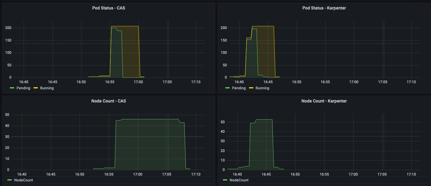
    CREATE OR REPLACE PROCEDURE merge_customer()
    AS $$
    BEGIN
    /*CREATING TEMP TABLE TO GET THE MOST LATEST RECORDS FOR UPDATES/NEW INSERTS*/
    CREATE TEMP TABLE merge_stg AS
    SELECT * FROM
    (
    SELECT *, DENSE_RANK() OVER (PARTITION BY c_custkey ORDER BY last_updated_ts DESC ) AS rnk
    FROM customer_stg
    )
    WHERE rnk = 1 AND metadata$action = 'INSERT';
    /* DELETING FROM THE BASE TABLE USING THE CDC STAGING TABLE ALL THE RECORDS MARKED AS DELETES OR UPDATES*/
    DELETE FROM customer
    USING customer_stg
    WHERE customer.c_custkey = customer_stg.c_custkey;
    /*INSERTING NEW/UPDATED RECORDS IN THE BASE TABLE*/ 
    INSERT INTO customer
    SELECT c_custkey, c_name, c_address, c_nationkey, c_phone, c_acctbal, c_mktsegment, c_comment
    FROM merge_stg;
    truncate customer_stg;
    END;
    $$ LANGUAGE plpgsql;

    For example, let’s look at the before and after states of the customer table when there’s been a change in data for a particular customer.

    The following screenshot shows the new changes recorded in the customer_stg table for c_custkey = 74360.
    merge-process-new-changes
    We can see two records for a customer with c_custkey=74360 one with metadata$action as DELETE and one with metadata$action as INSERT. That means the record with c_custkey was updated at the source and these changes need to be applied to the target customer table in Amazon Redshift.

    The following screenshot shows the current state of the customer table before these changes have been merged using the preceding stored procedure:
    merge-process-current-state

  6. Now, to update the target table, we can run the stored procedure as follows: CALL merge_customer()The following screenshot shows the final state of the target table after the stored procedure is complete.
    merge-process-after-sp

Run the stored procedure on a schedule

You can also run the stored procedure on a schedule via Amazon EventBridge. The scheduling steps are as follows:

  1. On the EventBridge console, choose Create rule.
    sp-schedule-1
  2. For Name, enter a meaningful name, for example, Trigger-Snowflake-Redshift-CDC-Merge.
  3. For Event bus, choose default.
  4. For Rule Type, select Schedule.
  5. Choose Next.
    sp-schedule-step-5
  6. For Schedule pattern, select A schedule that runs at a regular rate, such as every 10 minutes.
  7. For Rate expression, enter Value as 5 and choose Unit as Minutes.
  8. Choose Next.
    sp-schedule-step-8
  9. For Target types, choose AWS service.
  10. For Select a Target, choose Redshift cluster.
  11. For Cluster, choose the Amazon Redshift cluster identifier.
  12. For Database name, choose dev.
  13. For Database user, enter a user name with access to run the stored procedure. It uses temporary credentials to authenticate.
  14. Optionally, you can also use AWS Secrets Manager for authentication.
  15. For SQL statement, enter CALL merge_customer().
  16. For Execution role, select Create a new role for this specific resource.
  17. Choose Next.
    sp-schedule-step-17
  18. Review the rule parameters and choose Create rule.

After the rule has been created, it automatically triggers the stored procedure in Amazon Redshift every 5 minutes to merge the CDC data into the target table.

Configure Amazon Redshift to share the identified data with AWS Data Exchange

Now that you have the data stored inside Amazon Redshift, you can publish it to customers using AWS Data Exchange.

  1. In Amazon Redshift, using any query editor, create the data share and add the tables to be shared:
    CREATE DATASHARE salesshare MANAGEDBY ADX;
    ALTER DATASHARE salesshare ADD SCHEMA tpch_sf1;
    ALTER DATASHARE salesshare ADD TABLE tpch_sf1.customer;

    ADX-step1

  2. On the AWS Data Exchange console, create your dataset.
  3. Select Amazon Redshift datashare.
    ADX-step3-create-datashare
  4. Create a revision in the dataset.
    ADX-step4-create-revision
  5. Add assets to the revision (in this case, the Amazon Redshift data share).
    ADX-addassets
  6. Finalize the revision.
    ADX-step-6-finalizerevision

After you create the dataset, you can publish it to the public catalog or directly to customers as a private product. For instructions on how to create and publish products, refer to NEW – AWS Data Exchange for Amazon Redshift

Clean up

To avoid incurring future charges, complete the following steps:

  1. Delete the CloudFormation stack used to create the Redshift Auto Loader.
  2. Delete the Amazon Redshift cluster created for this demonstration.
  3. If you were using an existing cluster, drop the created external table and external schema.
  4. Delete the S3 bucket you created.
  5. Delete the Snowflake objects you created.

Conclusion

In this post, we demonstrated how you can set up a fully integrated process that continuously replicates data from Snowflake to Amazon Redshift and then uses Amazon Redshift to offer data to downstream clients over AWS Data Exchange. You can use the same architecture for other purposes, such as sharing data with other Amazon Redshift clusters within the same account, cross-accounts, or even cross-Regions if needed.


About the Authors

Raks KhareRaks Khare is an Analytics Specialist Solutions Architect at AWS based out of Pennsylvania. He helps customers architect data analytics solutions at scale on the AWS platform.

Ekta Ahuja is a Senior Analytics Specialist Solutions Architect at AWS. She is passionate about helping customers build scalable and robust data and analytics solutions. Before AWS, she worked in several different data engineering and analytics roles. Outside of work, she enjoys baking, traveling, and board games.

Tahir Aziz is an Analytics Solution Architect at AWS. He has worked with building data warehouses and big data solutions for over 13 years. He loves to help customers design end-to-end analytics solutions on AWS. Outside of work, he enjoys traveling
and cooking.

Ahmed Shehata is a Senior Analytics Specialist Solutions Architect at AWS based on Toronto. He has more than two decades of experience helping customers modernize their data platforms, Ahmed is passionate about helping customers build efficient, performant and scalable Analytic solutions.

Use Karpenter to speed up Amazon EMR on EKS autoscaling

Post Syndicated from Changbin Gong original https://aws.amazon.com/blogs/big-data/use-karpenter-to-speed-up-amazon-emr-on-eks-autoscaling/

Amazon EMR on Amazon EKS is a deployment option for Amazon EMR that allows organizations to run Apache Spark on Amazon Elastic Kubernetes Service (Amazon EKS). With EMR on EKS, the Spark jobs run on the Amazon EMR runtime for Apache Spark. This increases the performance of your Spark jobs so that they run faster and cost less than open source Apache Spark. Also, you can run Amazon EMR-based Apache Spark applications with other types of applications on the same EKS cluster to improve resource utilization and simplify infrastructure management.

Karpenter was introduced at AWS re:Invent 2021 to provide a dynamic, high performance, open-source cluster auto scaling solution for Kubernetes. It automatically provisions new nodes in response to unschedulable pods. It observes the aggregate resource requests of unscheduled pods and makes decisions to launch new nodes and terminate stop them to reduce scheduling latencies as well as infrastructure costs.

To configure Karpenter, you create provisioners that define how Karpenter manages the pods that are pending and expires nodes. Although most use cases are addressed with a single provisioner, multiple provisioners are useful in multi-tenant use cases such as isolating nodes for billing, using different node constraints (such as no GPUs for a team), or using different deprovisioning settings. Karpenter launches nodes with minimal compute resources to fit un-schedulable pods for efficient binpacking. It works in tandem with the Kubernetes scheduler to bind un-schedulable pods to the new nodes that are provisioned. The following diagram illustrates how it works.

This post shows how to integrate Karpenter into your EMR on EKS architecture to achieve faster and capacity-aware auto scaling capabilities to speed up your big data and machine learning (ML) workloads while reducing costs. We run the same workload using both Cluster Autoscaler and Karpenter, to see some of the improvements we discuss in the next section.

Improvements compared to Cluster Autoscaler

Like Karpenter, Kubernetes Cluster Autoscaler (CAS) is designed to add nodes when requests come in to run pods that can’t be met by current capacity. Cluster Autoscaler is part of the Kubernetes project, with implementations by major Kubernetes cloud providers. By taking a fresh look at provisioning, Karpenter offers the following improvements:

  • No node group management overhead – Because you have different resource requirements for different Spark workloads along with other workloads in your EKS cluster, you need to create separate node groups that can meet your requirements, like instance sizes, Availability Zones, and purchase options. This can quickly grow to tens and hundreds of node groups, which adds additional management overhead. Karpenter manages each instance directly, without the use of additional orchestration mechanisms like node groups, taking a group-less approach by calling the EC2 Fleet API directly to provision nodes. This allows Karpenter to use diverse instance types, Availability Zones, and purchase options by simply creating a single provisioner, as shown in the following figure.
  • Quick retries – If the Amazon Elastic Compute Cloud (Amazon EC2) capacity isn’t available, Karpenter can retry in milliseconds instead of minutes. This is can be a really useful if you’re using EC2 Spot Instances and you’re unable to get capacity to specific instance types.
  • Designed to handle full flexibility of the cloud – Karpenter has the ability to efficiently address the full range of instance types available through AWS. Cluster Autoscaler wasn’t originally built with the flexibility to handle hundreds of instance types, Availability Zones, and purchase options. We recommend being as flexible as you can be to enable Karpenter get the just-in-time capacity you need.
  • Improves the overall node utilization by binpacking – Karpenter batches pending pods and then binpacks them based on CPU, memory, and GPUs required, taking into account node overhead (for example, daemon set resources required). After the pods are binpacked on the most efficient instance type, Karpenter takes other instance types that are similar or larger than the most efficient packing, and passes the instance type options to an API called EC2 Fleet, following some of the best practices of instance diversification to improve the chances of getting the request capacity.

Best practices using Karpenter with EMR on EKS

For general best practices with Karpenter, refer to Karpenter Best Practices. The following are additional things to consider with EMR on EKS:

  • Avoid inter-AZ data transfer cost by either configuring the Karpenter provisioner to launch in a single Availability Zone or use node selector or affinity and anti-affinity to schedule the driver and the executors of the same job to a single Availability Zone. See the following code:
    nodeSelector:
      topology.kubernetes.io/zone: us-east-1a

  • Cost optimize Spark workloads using EC2 Spot Instances for executors and On-Demand Instances for the driver by using the node selector with the label karpenter.sh/capacity-type in the pod templates. We recommend using pod templates to specify driver pods to run on On-Demand Instances and executor pods to run on Spot Instances. This allows you to consolidate provisioner specs because you don’t need two specs per job type. It also follows the best practice of using customization defined on workload types and to keep provisioner specs to support a broader number of use cases.
  • When using EC2 Spot Instances, maximize the instance diversification in the provisioner configuration to adhere to the best practices. To select suitable instance types, you can use the ec2-instance-selector, a CLI tool and go library that recommends instance types based on resource criteria like vCPUs and memory.

Solution overview

This post provides an example of how to set up both Cluster Autoscaler and Karpenter in an EKS cluster and compare the auto scaling improvements by running a sample EMR on EKS workload.

The following diagram illustrates the architecture of this solution.

We use the Transaction Processing Performance Council-Decision Support (TPC-DS), a decision support benchmark to sequentially run three Spark SQL queries (q70-v2.4, q82-v2.4, q64-v2.4) with a fixed number of 50 executors, against 17.7 billion records, approximately 924 GB compressed data in Parquet file format. For more details on TPC-DS, refer to the eks-spark-benchmark GitHub repo.

We submit the same job with different Spark driver and executor specs to mimic different jobs solely to observe the auto scaling behavior and binpacking. We recommend you right-size your Spark executors based on the workload characteristics for production workloads.

The following code is an example Spark configuration that results in pod spec requests of 4 vCPU and 15 GB:

--conf spark.executor.instances=50 --conf spark.driver.cores=4 --conf spark.driver.memory=10g --conf spark.driver.memoryOverhead=5g --conf spark.executor.cores=4 --conf spark.executor.memory=10g  --conf spark.executor.memoryOverhead=5g

We use pod templates to schedule Spark drivers on On-Demand Instances and executors on EC2 Spot Instances (which can save up to 90% over On-Demand Instance prices). Spark’s inherent resiliency has the driver launch new executors to replace the ones that fail due to Spot interruptions. See the following code:

apiVersion: v1
kind: Pod
spec:
  nodeSelector:
    karpenter.sh/capacity-type: spot
  containers:
  - name: spark-kubernetes-executor


apiVersion: v1
kind: Pod
spec:
  nodeSelector:
    karpenter.sh/capacity-type: on-demand
  containers:
  - name: spark-kubernetes-driver

Prerequisites

We use an AWS Cloud9 IDE to run all the instructions throughout this post.

To create your IDE, run the following commands in AWS CloudShell. The default Region is us-east-1, but you can change it if needed.

# clone the repo
git clone https://github.com/black-mirror-1/karpenter-for-emr-on-eks.git
cd karpenter-for-emr-on-eks
./setup/create-cloud9-ide.sh

Navigate to the AWS Cloud9 IDE using the URL from the output of the script.

Install tools on the AWS Cloud9 IDE

Install the following tools required on the AWS Cloud9 environment by the running a script:

Run the following instructions in your AWS Cloud9 environment and not CloudShell.

  1. Clone the GitHub repository:
    cd ~/environment
    git clone https://github.com/black-mirror-1/karpenter-for-emr-on-eks.git
    cd ~/environment/karpenter-for-emr-on-eks

  2. Set up the required environment variables. Feel free to adjust the following code according to your needs:
    # Install envsubst (from GNU gettext utilities) and bash-completion
    sudo yum -y install jq gettext bash-completion moreutils
    
    # Setup env variables required
    export EKSCLUSTER_NAME=aws-blog
    export EKS_VERSION="1.23"
    # get the link to the same version as EKS from here https://docs.aws.amazon.com/eks/latest/userguide/install-kubectl.html
    export KUBECTL_URL="https://s3.us-west-2.amazonaws.com/amazon-eks/1.23.7/2022-06-29/bin/linux/amd64/kubectl"
    export HELM_VERSION="v3.9.4"
    export KARPENTER_VERSION="v0.18.1"
    # get the most recent matching version of the Cluster Autoscaler from here https://github.com/kubernetes/autoscaler/releases
    export CAS_VERSION="v1.23.1"

  3. Install the AWS Cloud9 CLI tools:
    cd ~/environment/karpenter-for-emr-on-eks
    ./setup/c9-install-tools.sh

Provision the infrastructure

We set up the following resources using the provision infrastructure script:

  1. Create the EMR on EKS and Karpenter infrastructure:
    cd ~/environment/karpenter-for-emr-on-eks
    ./setup/create-eks-emr-infra.sh

  2. Validate the setup:
    # Should have results that are running
    kubectl get nodes
    kubectl get pods -n karpenter
    kubectl get po -n kube-system -l app.kubernetes.io/instance=cluster-autoscaler
    kubectl get po -n prometheus

Understanding Karpenter configurations

Because the sample workload has driver and executor specs that are of different sizes, we have identified the instances from c5, c5a, c5d, c5ad, c6a, m4, m5, m5a, m5d, m5ad, and m6a families of sizes 2xlarge, 4xlarge, 8xlarge, and 9xlarge for our workload using the amazon-ec2-instance-selector CLI. With CAS, we need to create a total of 12 node groups, as shown in eksctl-config.yaml, but can define the same constraints in Karpenter with a single provisioner, as shown in the following code:

apiVersion: karpenter.sh/v1alpha5
kind: Provisioner
metadata:
  name: default
spec:
  provider:
    launchTemplate: {EKSCLUSTER_NAME}-karpenter-launchtemplate
    subnetSelector:
      karpenter.sh/discovery: {EKSCLUSTER_NAME}
  labels:
    app: kspark
  requirements:
    - key: "karpenter.sh/capacity-type"
      operator: In
      values: ["on-demand","spot"]
    - key: "kubernetes.io/arch" 
      operator: In
      values: ["amd64"]
    - key: karpenter.k8s.aws/instance-family
      operator: In
      values: [c5, c5a, c5d, c5ad, m5, c6a]
    - key: karpenter.k8s.aws/instance-size
      operator: In
      values: [2xlarge, 4xlarge, 8xlarge, 9xlarge]
    - key: "topology.kubernetes.io/zone"
      operator: In
      values: ["{AWS_REGION}a"]

  limits:
    resources:
      cpu: "2000"

  ttlSecondsAfterEmpty: 30

We have set up both auto scalers to scale down nodes that are empty for 30 seconds using ttlSecondsAfterEmpty in Karpenter and --scale-down-unneeded-time in CAS.

Karpenter by design will try to achieve the most efficient packing of the pods on a node based on CPU, memory, and GPUs required.

Run a sample workload

To run a sample workload, complete the following steps:

  1. Lets review the AWS Command Line Interface (AWS CLI) command to submit a sample job:
    aws emr-containers start-job-run \
      --virtual-cluster-id $VIRTUAL_CLUSTER_ID \
      --name karpenter-benchmark-${CORES}vcpu-${MEMORY}gb  \
      --execution-role-arn $EMR_ROLE_ARN \
      --release-label emr-6.5.0-latest \
      --job-driver '{
      "sparkSubmitJobDriver": {
          "entryPoint": "local:///usr/lib/spark/examples/jars/eks-spark-benchmark-assembly-1.0.jar",
          "entryPointArguments":["s3://blogpost-sparkoneks-us-east-1/blog/BLOG_TPCDS-TEST-3T-partitioned","s3://'$S3BUCKET'/EMRONEKS_TPCDS-TEST-3T-RESULT-KA","/opt/tpcds-kit/tools","parquet","3000","1","false","q70-v2.4,q82-v2.4,q64-v2.4","true"],
          "sparkSubmitParameters": "--class com.amazonaws.eks.tpcds.BenchmarkSQL --conf spark.executor.instances=50 --conf spark.driver.cores='$CORES' --conf spark.driver.memory='$EXEC_MEMORY'g --conf spark.executor.cores='$CORES' --conf spark.executor.memory='$EXEC_MEMORY'g"}}' \
      --configuration-overrides '{
        "applicationConfiguration": [
          {
            "classification": "spark-defaults", 
            "properties": {
              "spark.kubernetes.node.selector.app": "kspark",
              "spark.kubernetes.node.selector.topology.kubernetes.io/zone": "'${AWS_REGION}'a",
    
              "spark.kubernetes.container.image":  "'$ECR_URL'/eks-spark-benchmark:emr6.5",
              "spark.kubernetes.driver.podTemplateFile": "s3://'$S3BUCKET'/pod-template/karpenter-driver-pod-template.yaml",
              "spark.kubernetes.executor.podTemplateFile": "s3://'$S3BUCKET'/pod-template/karpenter-executor-pod-template.yaml",
              "spark.network.timeout": "2000s",
              "spark.executor.heartbeatInterval": "300s",
              "spark.kubernetes.executor.limit.cores": "'$CORES'",
              "spark.executor.memoryOverhead": "'$MEMORY_OVERHEAD'G",
              "spark.driver.memoryOverhead": "'$MEMORY_OVERHEAD'G",
              "spark.kubernetes.executor.podNamePrefix": "karpenter-'$CORES'vcpu-'$MEMORY'gb",
              "spark.executor.defaultJavaOptions": "-verbose:gc -XX:+UseG1GC",
              "spark.driver.defaultJavaOptions": "-verbose:gc -XX:+UseG1GC",
    
              "spark.ui.prometheus.enabled":"true",
              "spark.executor.processTreeMetrics.enabled":"true",
              "spark.kubernetes.driver.annotation.prometheus.io/scrape":"true",
              "spark.kubernetes.driver.annotation.prometheus.io/path":"/metrics/executors/prometheus/",
              "spark.kubernetes.driver.annotation.prometheus.io/port":"4040",
              "spark.kubernetes.driver.service.annotation.prometheus.io/scrape":"true",
              "spark.kubernetes.driver.service.annotation.prometheus.io/path":"/metrics/driver/prometheus/",
              "spark.kubernetes.driver.service.annotation.prometheus.io/port":"4040",
              "spark.metrics.conf.*.sink.prometheusServlet.class":"org.apache.spark.metrics.sink.PrometheusServlet",
              "spark.metrics.conf.*.sink.prometheusServlet.path":"/metrics/driver/prometheus/",
              "spark.metrics.conf.master.sink.prometheusServlet.path":"/metrics/master/prometheus/",
              "spark.metrics.conf.applications.sink.prometheusServlet.path":"/metrics/applications/prometheus/"
             }}
        ]}'

  2. Submit four jobs with different driver and executor vCPUs and memory sizes on Karpenter:
    # the arguments are vcpus and memory
    export EMRCLUSTER_NAME=${EKSCLUSTER_NAME}-emr
    ./sample-workloads/emr6.5-tpcds-karpenter.sh 4 7
    ./sample-workloads/emr6.5-tpcds-karpenter.sh 8 15
    ./sample-workloads/emr6.5-tpcds-karpenter.sh 4 15
    ./sample-workloads/emr6.5-tpcds-karpenter.sh 8 31 

  3. To monitor the pods’s autoscaling status in real time, open a new terminal in Cloud9 IDE and run the following command (nothing is returned at the start):
    watch -n1 "kubectl get pod -n emr-karpenter"

  4. Observe the EC2 instance and node auto scaling status in a second terminal tab by running the following command (by design, Karpenter schedules in Availability Zone a):
    watch -n1 "kubectl get node --label-columns=node.kubernetes.io/instance-type,karpenter.sh/capacity-type,topology.kubernetes.io/zone,app -l app=kspark"

Compare with Cluster Autoscaler (Optional)

We have set up Cluster Autoscaler during the infrastructure setup step with the following configuration:

  • Launch EC2 nodes in Availability Zone b
  • Contain 12 node groups (6 each for On-Demand and Spot)
  • Scale down unneeded nodes after 30 seconds with --scale-down-unneeded-time
  • Use the least-waste expander on CAS, which can select the node group that will have the least idle CPU for binpacking efficiency
  1. Submit four jobs with different driver and executor vCPUs and memory sizes on CAS:
    # the arguments are vcpus and memory
    ./sample-workloads/emr6.5-tpcds-ca.sh 4 7
    ./sample-workloads/emr6.5-tpcds-ca.sh 8 15
    ./sample-workloads/emr6.5-tpcds-ca.sh 4 15
    ./sample-workloads/emr6.5-tpcds-ca.sh 8 31

  2. To monitor the pods’s autoscaling status in real time, open a new terminal in Cloud9 IDE and run the following command (nothing is returned at the start):
    watch -n1 "kubectl get pod -n emr-ca"

  3. Observe the EC2 instance and node auto scaling status in a second terminal tab by running the following command (by design, CAS schedules in Availability Zone b):
    watch -n1 "kubectl get node --label-columns=node.kubernetes.io/instance-type,eks.amazonaws.com/capacityType,topology.kubernetes.io/zone,app -l app=caspark"

Observations

The time from pod creation to being scheduled on average is less with Karpenter than CAS, as shown in the following figure; you can see a noticeable difference when you run large scale workloads.

As shown in the following figures, as the jobs were completed, Karpenter was able to scale down the nodes that aren’t needed within seconds. In contrast, CAS takes minutes, because it sends a signal to the node groups, adding additional latency. This in turn helps reduce overall costs by reducing the number of seconds unneeded EC2 instances are running.

Clean up

To clean up your environment, delete all the resources created in reverse order by running the cleanup script:

export EKSCLUSTER_NAME=aws-blog
cd ~/environment/karpenter-for-emr-on-eks
./setup/cleanup.sh

Conclusion

In this post, we showed you how to use Karpenter to simplify EKS node provisioning, and speed up auto scaling of EMR on EKS workloads. We encourage you to try Karpenter and provide any feedback by creating a GitHub issue.

Further reading


About the Authors

Changbin Gong is a Principal Solutions Architect at Amazon Web Services. He engages with customers to create innovative solutions that address customer business problems and accelerate the adoption of AWS services. In his spare time, Changbin enjoys reading, running, and traveling.

Sandeep Palavalasa is a Sr. Specialist Containers SA at Amazon Web Services. He is a software technology leader with over 12 years of experience in building large-scale, distributed software systems. His professional career started with a focus on monitoring and observability and he has a strong cloud architecture background. He likes working on distributed systems and is excited to talk about microservice architecture design. His current interests are in the areas of container services and serverless technologies.

Match Cutting at Netflix: Finding Cuts with Smooth Visual Transitions

Post Syndicated from Netflix Technology Blog original https://netflixtechblog.com/match-cutting-at-netflix-finding-cuts-with-smooth-visual-transitions-31c3fc14ae59

By Boris Chen, Kelli Griggs, Amir Ziai, Yuchen Xie, Becky Tucker, Vi Iyengar, Ritwik Kumar

Creating Media with Machine Learning episode 1

Introduction

At Netflix, part of what we do is build tools to help our creatives make exciting videos to share with the world. Today, we’d like to share some of the work we’ve been doing on match cuts.

In film, a match cut is a transition between two shots that uses similar visual framing, composition, or action to fluidly bring the viewer from one scene to the next. It is a powerful visual storytelling tool used to create a connection between two scenes.

[Spoiler alert] consider this scene from Squid Game:

The players voted to leave the game after red-light green-light, and are back in the real world. After a rough night, Gi Hung finds another calling card and considers returning to the game. As he waits for the van, a series of powerful match cuts begins, showing the other characters doing the exact same thing. We never see their stories, but because of the way it was edited, we instinctively understand that they made the same decision. This creates an emotional bond between these characters and ties them together.

A more common example is a cut from an older person to a younger person (or vice versa), usually used to signify a flashback (or flashforward). This is sometimes used to develop the story of a character. This could be done with words verbalized by a narrator or a character, but that could ruin the flow of a film, and it is not nearly as elegant as a single well executed match cut.

An example from Oldboy. A child wipes their eyes on a train, which cuts to a flashback of a younger child also wiping their eyes. We as the viewer understand that the next scene must be from this child’s upbringing.
A flashforward from a young Indian Jones to an older Indian Jones conveys to the viewer that what we just saw about his childhood makes him the person he is today.

Here is one of the most famous examples from Stanley Kubrik’s 2001: A Space Odyssey. A bone is thrown into the air. As it spins, a single instantaneous cut brings the viewer from the prehistoric first act of the film into the futuristic second act. This highly artistic cut suggests that mankind’s evolution from primates to space technology is natural and inevitable.

Match cutting is also widely used outside of film. They can be found in trailers, like this sequence of shots from the trailer for Firefly Lane.

Match cutting is considered one of the most difficult video editing techniques, because finding a pair of shots that match can take days, if not weeks. An editor typically watches one or more long-form videos and relies on memory or manual tagging to identify shots that would match to a reference shot observed earlier.

A typical two hour movie might have around 2,000 shots, which means there are roughly 2 million pairs of shots to compare. It quickly becomes impossible to do this many comparisons manually, especially when trying to find match cuts across a 10 episode series, or multiple seasons of a show, or across multiple different shows.

What’s needed in the art of match cutting is tools to help editors find shots that match well together, which is what we’ve started building.

Our Initial Approach

Collecting training data is much more difficult compared to more common computer vision tasks. While some types of match cuts are more obvious, others are more subtle and subjective.

For instance, consider this match cut from Lawrence of Arabia. A man blows a match out, which cuts into a long, silent shot of a sunrise. It’s difficult to explain why this works, but many creatives recognize this as one of the greatest match cuts in film.

To avoid such complexities, we started with a more well-defined flavor of match cuts: ones where the visual framing of a person is aligned, aka frame matching. This came from the intuition of our video editors, who said that a large percentage of match cuts are centered around matching the silhouettes of people.

Frame matches from Stranger Things.

We tried several approaches, but ultimately what worked well for frame matching was instance segmentation. The output of segmentation models gives us a pixel mask of which pixels belong to which objects. We take the segmentation output of two different frames, and compute intersection over union (IoU) between the two. We then rank pairs using IoU and surface high-scoring pairs as candidates.

A few other details were added along the way. To deal with not having to brute force every single pair of frames, we only took the middle frame of each shot, since many frames look visually similar within a single shot. To deal with similar frames from different shots, we performed image deduplication upfront. In our early research, we simply discarded any mask that wasn’t a person to keep things simple. Later on, we added non-person masks back to be able to find frame match cuts of animals and objects.

A series of frame match cuts of animals from Our planet.
Object frame match from Paddington 2.

Action and Motion

At this point, we decided to move onto a second flavor of match cutting: action matching. This type of match cut involves the continuation of motion of object or person A’s motion to the object or person B’s motion in another shot (A and B can be the same so long as the background, clothing, time of day, or some other attribute changes between the two shots).

An action match cut from Resident Evil.
A series of action mat cuts from Extraction, Red Notice, Sandman, Glow, Arcane, Sea Beast, and Royalteen.

To capture this type of information, we had to move beyond image level and extend into video understanding, action recognition, and motion. Optical flow is a common technique used to capture motion, so that’s what we tried first.

Consider the following shots and the corresponding optical flow representations:

Shots from The Umbrella Academy.

A red pixel means the pixel is moving to the right. A blue pixel means the pixel is moving to the left. The intensity of the color represents the magnitude of the motion. The optical flow representations on the right show a temporal average of all the frames. While averaging can be a simple way to match the dimensionality of the data for clips of different duration, the downside is that some valuable information is lost.

When we substituted optical flow in as the shot representations (replacing instance segmentation masks) and used cosine similarity in place of IoU, we found some interesting results.

Shots from The Umbrella Academy.

We saw that a large percentage of the top matches were actually matching based on similar camera movement. In the example above, purple in the optical flow diagram means the pixel is moving up. This wasn’t what we were expecting, but it made sense after we saw the results. For most shots, the number of background pixels outnumbers the number of foreground pixels. Therefore, it’s not hard to see why a generic similarity metric giving equal weight to each pixel would surface many shots with similar camera movement.

Here are a couple of matches found using this method:

Camera movement match cut from Bridgerton.
Camera movement match cut from Blood & Water.

While this wasn’t what we were initially looking for, our video editors were delighted by this output, so we decided to ship this feature as is.

Our research into true action matching still remains as future work, where we hope to leverage action recognition and foreground-background segmentation.

Match cutting system

The two flavors of match cutting we explored share a number of common components. We realized that we can break the process of finding matching pairs into five steps.

System diagram for match cutting. The input is a video file (film or series episode) and the output is K match cut candidates of the desired flavor. Each colored square represents a different shot. The original input video is broken into a sequence of shots in step 1. In Step 2, duplicate shots are removed (in this example the fourth shot is removed). In step 3, we compute a representation of each shot depending on the flavor of match cutting that we’re interested in. In step 4 we enumerate all pairs and compute a score for each pair. Finally, in step 5, we sort pairs and extract the top K (e.g. K=3 in this illustration).

1- Shot segmentation

Movies, or episodes in a series, consist of a number of scenes. Scenes typically transpire in a single location and continuous time. Each scene can be one or many shots- where a shot is defined as a sequence of frames between two cuts. Shots are a very natural unit for match cutting, and our first task was to segment a movie into shots.

Stranger Things season 1 episode 1 broken down into scenes and shots.

Shots are typically a few seconds long, but can be much shorter (less than a second) or minutes long in rare cases. Detecting shot boundaries is largely a visual task and very accurate computer vision algorithms have been designed and are available. We used an in-house shot segmentation algorithm, but similar results can be achieved with open source solutions such as PySceneDetect and TransNet v2.

2- Shot deduplication

Our early attempts surfaced many near-duplicate shots. Imagine two people having a conversation in a scene. It’s common to cut back and forth as each character delivers a line.

A dialogue sequence from Stranger Things Season 1.

These near-duplicate shots are not very interesting for match cutting and we quickly realized that we need to filter them out. Given a sequence of shots, we identified groups of near-duplicate shots and only retained the earliest shot from each group.

Identifying near-duplicate shots

Given the following pair of shots, how do you determine if the two are near-duplicates?

Near-duplicate shots from Stranger Things.

You would probably inspect the two visually and look for differences in colors, presence of characters and objects, poses, and so on. We can use computer vision algorithms to mimic this approach. Given a shot, we can use an algorithm that’s been trained on a large dataset of videos (or images) and can describe it using a vector of numbers.

An encoder represents a shot from Stranger Things using a vector of numbers.

Given this algorithm (typically called an encoder in this context), we can extract a vector (aka embedding) for a pair of shots, and compute how similar they are. The vectors that such encoders produce tend to be high dimensional (hundreds or thousands of dimensions).

To build some intuition for this process, let’s look at a contrived example with 2 dimensional vectors.

Three shots from Stranger Things and the corresponding vector representations.

The following is a depiction of these vectors:

Shots 1 and 3 are near-duplicates. The vectors representing these shots are close to each other. All shots are from Stranger Things.

Shots 1 and 3 are near-duplicates and we see that vectors 1 and 3 are close to each other. We can quantify closeness between a pair of vectors using cosine similarity, which is a value between -1 and 1. Vectors with cosine similarity close to 1 are considered similar.

The following table shows the cosine similarity between pairs of shots:

Shots 1 and 3 have high cosine similarity (0.96) and are considered near-duplicates while shots 1 and 2 have a smaller cosine similarity value (0.42) and are not considered near-duplicates. Note that the cosine similarity of a vector with itself is 1 (i.e. it’s perfectly similar to itself) and that cosine similarity is commutative. All shots are from Stranger Things.

This approach helps us to formalize a concrete algorithmic notion of similarity.

3- Compute representations

Steps 1 and 2 are agnostic to the flavor of match cutting that we’re interested in finding. This step is meant for capturing the matching semantics that we are interested in. As we discussed earlier, for frame match cutting, this can be instance segmentation, and for camera movement, we can use optical flow.

However, there are many other possible options to represent each shot that can help us do the matching. These can be heuristically defined ahead of time based on our knowledge of the flavors, or can be learned from labeled data.

4- Compute pair scores

In this step, we compute a similarity score for all pairs. The similarity score function takes a pair of representations and produces a number. The higher this number, the more similar the pairs are deemed to be.

Steps 3 and 4 for a pair of shots from Stranger Things. In this example the representation is the person instance segmentation mask and the metric is IoU.

5- Extract top-K results

Similar to the first two steps, this step is also agnostic to the flavor. We simply rank pairs by the computed score in step 4, and take the top K (a parameter) pairs to be surfaced to our video editors.

Using this flexible abstraction, we have been able to explore many different options by picking different concrete implementations for steps 3 and 4.

Dataset

How well does this system work? To answer this question, we decided to collect a labeled dataset of approximately 20k labeled pairs. Each pair was annotated by 3 video editors. For frame match cutting, the three video editors were in perfect agreement (i.e. all three selected the same label) 84% of the time. For motion match cutting, which is a more nuanced and subjective task, perfect agreement was 75%.

We then took the majority label for each pair and used it to evaluate our model.

We started with 100 movies, which produced 128k shots and 8.2 billion unique pairs. This diagram depicts the process of reducing this set down to the final set of 19,305 pairs that were annotated.

Evaluation

Binary classification with frozen embeddings

With the above dataset with binary labels, we are armed to train our first model. We extracted fixed embeddings from a variety of image, video, and audio encoders (a model or algorithm that extracts a representation given a video clip) for each pair and then aggregated the results into a single feature vector to learn a classifier on top of.

We extracted fixed embeddings using the same encoder for each shot. Then we aggregated the embeddings and passed the aggregation results to a classification model.

We surface top ranking pairs to video editors. A high quality match cutting system places match cuts at the top of the list by producing higher scores. We used Average Precision (AP) as our evaluation metric. AP is an information retrieval metric that is suitable for ranking scenarios such as ours. AP ranges between 0 and 1, where higher values reflect a higher quality model.

The following table summarizes our results:

Reporting AP on the test set. Baseline is a random ranking of the pairs, which for AP is equivalent to the positive prevalence of each task in expectation.

EfficientNet7 and R(2+1)D perform best for frame and motion respectively.

Metric learning

A second approach we considered was metric learning. This approach gives us transformed embeddings which can be indexed and retrieved using Approximate Nearest Neighbor (ANN) methods.

Reporting AP on the test set. Baseline is a random ranking of the pairs similar to the previous section.

Leveraging ANN, we have been able to find matches across hundreds of shows (on the order of tens of millions of shots) in seconds.

If you’re interested in more technical details make sure you take a look at our preprint paper here.

Conclusion

There are many more ideas that have yet to be tried: other types of match cuts such as action, light, color, and sound, better representations, and end-to-end model training, just to name a few.

Match cuts from Partner Track.
An action match cut from Lost In Space and Cowboy Bebop.
A series of match cuts from 1899.

We’ve only scratched the surface of this work and will continue to build tools like this to empower our creatives. If this type of work interests you, we are always looking for collaboration opportunities and hiring great machine learning engineers, researchers, and interns to help build exciting tools.

We’ll leave you with this teaser for Firefly Lane, edited by Aly Parmelee, which was the first piece made with the help of the match cutting tool:


Match Cutting at Netflix: Finding Cuts with Smooth Visual Transitions was originally published in Netflix TechBlog on Medium, where people are continuing the conversation by highlighting and responding to this story.

Fall 2022 SOC reports now available with 154 services in scope

Post Syndicated from Andrew Najjar original https://aws.amazon.com/blogs/security/fall-2022-soc-reports-now-available-with-154-services-in-scope/

At Amazon Web Services (AWS), we’re committed to providing customers with continued assurance over the security, availability, and confidentiality of the AWS control environment. We’re proud to deliver the Fall 2022 System and Organizational Controls (SOC) 1, 2, and 3 reports, which cover April 1–September 30, 2022, to support our customers’ confidence in AWS services.

AWS has also updated the associated infrastructure supporting our in-scope products and services to reflect new edge locations, AWS Wavelength zones, and AWS Local Zones.

The Fall 2022 SOC reports include an additional seven services in scope, for a new total of 154 services. See the full list on our Services in Scope by Compliance Program page.

The following are the additional seven services now in scope for the Fall 2022 SOC reports:

Customers can download the Fall 2022 SOC reports through AWS Artifact in the AWS Management Console. You can also download the SOC 3 report as a PDF file from AWS.

AWS strives to bring services into the scope of its compliance programs to help you meet your architectural and regulatory needs. If there are additional AWS services that you would like to see added to the scope of our SOC reports (or other compliance programs), reach out to your AWS representatives.

As always, we value your feedback and questions. Feel free to reach out to the team through the Contact Us page. If you have feedback about this post, submit comments in the Comments section below.

Want more AWS Security how-to-content, news, and feature announcements? Follow us on Twitter.

Andrew Najjar

Andrew Najjar

Andrew is a Compliance Program Manager at Amazon Web Services. He leads multiple security and privacy initiatives within AWS and has 8 years of experience in security assurance. Andrew holds a master’s degree in information systems and bachelor’s degree in accounting from Indiana University. He is a CPA and AWS Certified Solution Architect – Associate.

ryan wilks

Ryan Wilks

Ryan is a Compliance Program Manager at Amazon Web Services. He leads multiple security and privacy initiatives within AWS. Ryan has 11 years of experience in information security and holds ITIL, CISM and CISA certifications.

Nathan Samuel

Nathan Samuel

Nathan is a Compliance Program Manager at Amazon Web Services. He leads multiple security and privacy initiatives within AWS. Nathan has a Bachelors of Commerce degree from the University of the Witwatersrand, South Africa and has 17 years’ experience in security assurance and holds the CISA, CRISC, CGEIT, CISM, CDPSE and Certified Internal Auditor certifications.

Fall 2022 SOC 2 Type 2 Privacy report now available

Post Syndicated from Nimesh Ravasa original https://aws.amazon.com/blogs/security/fall-2022-soc-2-type-2-privacy-report-now-available/

Your privacy considerations are at the core of our compliance work at Amazon Web Services (AWS), and we are focused on the protection of your content while using AWS services.

We are happy to announce that our Fall 2022 SOC 2 Type 2 Privacy report is now available. The report provides a third-party attestation of our system and the suitability of the design of our privacy controls. The SOC 2 Privacy Trust Service Criteria (TSC), developed by the American Institute of Certified Public Accountants (AICPA), establishes the criteria for evaluating controls that relate to how personal information is collected, used, retained, disclosed, and disposed of. For more information about our privacy commitments supporting the SOC 2 Type 2 report, see the AWS Customer Agreement.

The scope of the Fall 2022 SOC 2 Type 2 Privacy report includes information about how we handle the content that you upload to AWS, and how that content is protected across the services and locations that are in scope for the latest AWS SOC reports. AWS customers can download the SOC 2 Type 2 Privacy report through AWS Artifact in the AWS Management Console.

As always, we value your feedback and questions. Feel free to reach out to the compliance team through the AWS Compliance Contact Us page. If you have feedback about this post, submit comments in the Comments section below.

Want more AWS Security how-to-content, news, and feature announcements? Follow us on Twitter.

Nimesh Ravasa

Nimesh Ravasa

Nimesh is a Compliance Program Manager at Amazon Web Services. He leads multiple security and privacy initiatives within AWS. Nimesh has 14 years of experience in information security and holds CISSP, CISA, PMP, CSX, AWS Solution Architect – Associate, and AWS Security Specialty certifications.

Emma Zhang

Emma Zhang

Emma is a Compliance Program Manager at Amazon Web Services. She leads multiple process improvement projects across multiple compliance programs within AWS. Emma has 8 years of experience in risk management, IT risk assurance, and technology risk advisory.

Brownell Combs

Brownell Combs

Brownell is a Compliance Program Manager at Amazon Web Services. He leads multiple security and privacy initiatives within AWS. Brownell holds a Master of Science, Computer Science degree from the University of Virginia and a Bachelor of Science, Computer Science degree from Centre College. He has over 20 years of experience in Information Technology risk management and CISSP, CISA, and CRISC certifications.

Rapid7 and HashiCorp Partner to Secure Terraform-based Cloud Infrastructure Deployments

Post Syndicated from Clint Merrill original https://blog.rapid7.com/2022/11/17/rapid7-and-hashicorp-partner-to-secure-terraform-based-cloud-infrastructure-deployments/

Rapid7 and HashiCorp Partner to Secure Terraform-based Cloud Infrastructure Deployments

Welcome to the latest installment in our cloud security “shift-left” blog series. In our last post, we covered the importance of integrating cloud infrastructure security assessments into DevOps tools and enabling Infrastructure as Code (IaC) developers. This time, we’re focusing on Rapid7’s recent partnership with Hashicorp, ongoing support for scanning Terraform plans with our IaC security feature, and the recently released integration with Terraform Cloud & Enterprise run tasks.

HashiCorp Terraform and InsightCloudSec are a powerful combination

Rapid7 and HashiCorp Partner to Secure Terraform-based Cloud Infrastructure Deployments

There are countless reasons to adopt cloud infrastructure: hosting applications, compute workloads, data storage, virtual networking, governing identity and access control, and many other use-cases. We are spoiled for choice with the vast array of cloud resources and services designed to perform specific tasks, but each one requires specialized knowledge to configure it securely and interact with other resources. Additionally, resilient cloud applications typically leverage best-in-class features from multiple cloud service providers (CSPs) who compete with innovation, unique features and cost optimization. The more distributed your cloud resources are across providers, the more powerful it is to define them via IaC with a tool that can deploy to any provider.

HashiCorp Terraform is a widely-used open-source IaC tool, especially for supporting multi-cloud deployments. InsightCloudSec has the ability to scan Terraform plans destined for accounts in AWS, Azure or GCP. Rapid7 supports the key resource types for each of the three major cloud providers, and we are constantly expanding our coverage based on usage trends or as needed by our customers.

A major benefit of using InsightCloudSec for IaC security and compliance scans is that you can use the same Insight Compliance Pack for assessing runtime environments and IaC, rather than correlating policy definitions across different tools. This reduces the overhead of maintaining multiple policies and the associated rules across different tools and languages which can easily drift apart. We call this “One Policy”.

Terraform allows users to develop immutable cloud resource definitions as code in a common language for deployment to multiple cloud providers. When paired with InsightCloudSec, resource definitions can be assessed with a single set of security policies applied to both development and runtime environments—creating an optimized experience that delivers efficiency and convenience. To further power this union, Rapid7 has partnered with HashiCorp to develop a formal integration between Terraform Cloud and InsightCloudSec (ICS).

New integrations with HashiCorp Terraform Cloud and Terraform Enterprise run tasks

IaC developers create Terraform configurations using HashiCorp configuration language (HCL) and commit them to a source code repository such as Git. The Terraform configuration and the current infrastructure state are evaluated to generate a deployment plan—a preview of changes that will be made in the destination cloud account(s). By linking HCL configurations to collections of resources defined as workspaces in Terraform Cloud, deployment plans are generated and await approval to apply them. At this point, run tasks are used to invoke analysis of the plan, including security and compliance checks in external tools to inform or gate the approval step. This process can be managed through workflows on one of many supported CI/CD platforms; however, HashiCorp developed Terraform Cloud and Enterprise to govern, optimize and secure the process.

DevOps teams using Terraform Cloud to govern cloud infrastructure deployments can securely and reliably trigger a security and compliance assessment of a Terraform plan in ICS using a run task. We’ve worked with the team at HashiCorp to streamline the process of linking a run task to an IaC Configuration in ICS which defines the security policy (Insight Compliance Pack) that will be used to assess the Terraform plan.

Rapid7 and HashiCorp Partner to Secure Terraform-based Cloud Infrastructure Deployments

This investment is the latest step in our strategy at Rapid7 to directly support DevOps teams to apply IaC security using the tool of their choice. Terraform Cloud was at the top of our list for a formal integration given its prevalent use in the cloud infrastructure and application development community.

Ready to get started?

Configuring the new integrations with Terraform is a straightforward process, but let’s walk through it at a high level. Assuming you’ve configured your Terraform Cloud or Enterprise environment with workspaces to generate plans, we’ll show you how to link a Run Task to an IaC Configuration in ICS. Detailed instructions are available in the ICS Product Documentation.

Visit the Infrastructure as Code landing page and select the Configurations tab at the top. Any existing Configuration defined to support scanning Terraform plans can be linked to a run task.  Click the Action menu and select the “TFC/E Run Task Integrations” option.

Rapid7 and HashiCorp Partner to Secure Terraform-based Cloud Infrastructure Deployments

From there, you’ll generate an unique Endpoint URL and HMAC key used during the creation of the run task in Terraform Cloud to securely bind the two systems.

Rapid7 and HashiCorp Partner to Secure Terraform-based Cloud Infrastructure Deployments

Next, switch to the Terraform Cloud / Enterprise organization settings interface and create a run task. Copy/paste the Endpoint URL and HMAC key provided to you in ICS.

Rapid7 and HashiCorp Partner to Secure Terraform-based Cloud Infrastructure Deployments

After the run task is successfully created, you will need to associate it with a workspace before generating a plan and triggering it to test the end-to-end process.

During the run task execution, you’ll notice active communication between the two systems monitoring the state of the scan job in ICS and reporting back a final state as Passed, Failed, or Error (indicating the scan job didn’t successfully complete).

We’ve made this integration process simple and accessible to DevOps teams via ICS and Terraform Cloud without any custom API integration required. You can ensure IaC security and compliance scans in ICS are routinely applied to the approval step before Terraform plans are applied to a destination cloud environment.

Our DevOps-focused cloud security investment continues

Rapid7’s InsightCloudSec is proud to partner with HashiCorp to help fulfill the joint mission of making cloud infrastructure and application development and maintenance low cost, code-driven, repeatable, scalable and secure.

For more information , please visit HashiCorp’s partnership page.

Our next blog in the “shift-left” series will include an announcement and overview of a significant upgrade we’re making to our IaC scanning engine and the underlying technology we use to identify issues, pinpoint the location of the problem in code, and provide ‘Actionable Results’ to assist developers with remediation.

The collective thoughts of the interwebz