On July 28, 2026, MCP published its largest revision since launch, making the protocol core stateless and bringing remote MCP servers into alignment with AWS Well-Architected Framework best practices. The initialize handshake is gone, and so is the Mcp-Session-Id header that clients had to echo on every later request. Every request now carries its own protocol version and client context. A client’s first message can be the actual tool call, and any server instance can respond to it. If your MCP server was built for the session-based protocol, the sticky sessions, shared session stores, and custom observability plumbing it required are no longer necessary. If you run behind Amazon Bedrock AgentCore Gateway, protocol management and backward compatibility are handled for you. This post is for teams managing the full deployment stack themselves.
If a client wants to know what a server supports before calling it, a new server/discover method returns the supported protocol versions, capabilities, and identity in a single response. Servers must implement it per the MCP 2026-07-28 specification, but calling it is optional for the client.
This matters on AWS because the old design fought horizontal scaling. A session lived on whichever instance issued it. Running more than one instance meant either pinning clients with sticky routing or externalizing session state to a shared store. Both were correct for that protocol. With the new protocol, neither is required. This post maps the MCP 2026-07-28 specification against the Well-Architected Agentic AI Lens and recommends migrating, because the new protocol achieves natively what the old one could only achieve through compensating infrastructure.
One thing to settle up front, because it drives everything else: stateless describes the protocol, not your application. Stateful use cases still work.
Think of it as a coat check. Under the old protocol the server was a valet who remembered your face, which meant you had to keep dealing with that same valet and nobody else could help you. Now you get a numbered ticket, and any attendant can serve you because the ticket carries the reference. When a server needs continuity across calls, a tool returns an identifier for the stored state. The model includes that identifier on the calls that follow. The state stays in your datastore. The model carries only the key. This is ordinary REST discipline. It has an advantage over the old model. The identifier sits in the model’s context rather than hidden in a header. The model can reason about it and thread it across tools.
What changes in your architecture
The following table compares the deployment patterns the session-based protocol required against the patterns the stateless core now supports.
Before (session-based)
After (2026-07-28 stateless)
Elastic Load Balancing Application Load Balancer (ALB) stickiness so each session reaches the same instance.
Plain round-robin. Delete the stickiness configuration.
Session state in Amazon DynamoDB or Amazon ElastiCache.
No session store. Server-minted identifiers passed as tool arguments.
Parse request bodies at the gateway to route by method.
Route and throttle on the Mcp-Method and Mcp-Name headers.
AWS Lambda required workarounds for the stateful handshake.
AWS Lambda is a natural fit. Request in, response out.
Refetch tool lists per session. No caching story.
Cache with ttlMs and cacheScope, the protocol’s built-in freshness fields.
Bolt-on tracing per implementation. Proprietary protocol logging channel.
W3C Trace Context in _meta for distributed tracing. stderr or OpenTelemetry for logging. Protocol logging is deprecated.
Rely on stream resumption (Last-Event-ID) for broken responses.
Make tools idempotent. Clients re-issue broken calls.
Don’t delete yet if you serve 2025-era clients. The 2026-07-28 spec includes a backward-compatible lane that preserves session semantics for older clients. Your ALB stickiness rules and session store (DynamoDB/ElastiCache) must remain in place until you stop serving pre-2026-07-28 clients. Action: Instrument your gateway to log protocol version per request. Set a sunset date for the legacy lane and communicate it to client teams. Only decommission session infrastructure after traffic on the old version reaches zero. This guidance applies to session infrastructure built to compensate for the old protocol’s requirements. Managed hosts that offer session features by design for specific use cases are not in scope.
One behavioral change to plan for. Servers can no longer push a request to a client mid-call, which is how confirmations, sampling, and root queries used to work over a held-open stream. The spec replaces that pattern with Multi Round-Trip Requests (MRTR). A server that needs input returns an input_required result containing an inputRequests map. This map holds elicitations, sampling calls, or root queries, and an opaque requestState token. The client fulfills the requests, then re-sends the original call with inputResponses and the echoed requestState. Any instance can pick that up because requestState carries all the context the server needs to resume. No shared session store is required. The server does not hold the connection open. This is what makes the pattern work on AWS Lambda.
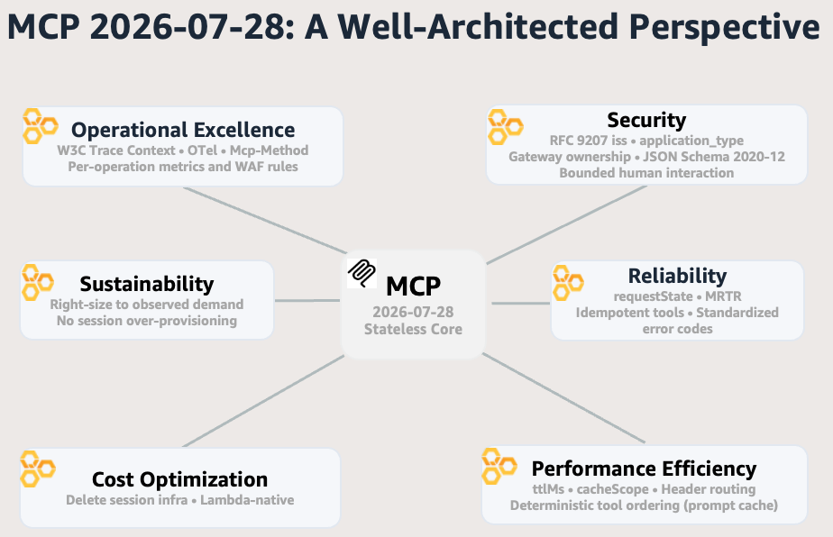
Figure 1: How the MCP 2026-07-28 specification maps to the Well-Architected Agentic AI Lens pillars
Operational excellence. The Lens identifies observability as the foundation for operating agents. If you cannot trace a decision end to end, you cannot debug, optimize, or audit it. The 2026-07-28 spec builds observability into the protocol itself. Three changes make this concrete:
Tracing. Every request carries W3C Trace Context keys in _meta (traceparent, tracestate, baggage), so it traces end to end through any OpenTelemetry-compatible backend, including Amazon CloudWatch. The Lens prescribes end-to-end tracing and telemetry for agent operations.
Operational signals without body parsing. The Mcp-Method and Mcp-Name headers expose the operation type on every POST, and every response carries a required resultType field (complete or input_required). Gateways and observability tools get unambiguous per-operation signals for metrics, alarms, and AWS WAF rules without inspecting payloads. The result directly addresses the Lens recommendation for implementing metrics and monitoring for agent-specific patterns.
Security. The Lens treats agent security as harder than traditional service security: agents act autonomously with delegated credentials, and their inputs (including state identifiers) are visible to, and potentially manipulable by, the model. MCP’s 2026-07-28 spec hardens the protocol surface against these risks. Five changes strengthen the security posture:
Client type declaration. Clients must declare application_type at registration so a desktop or CLI client is not mistaken for a web app, verifying authentication mechanisms match the client’s security profile. The same Lens best practice applies: strong authentication for agent identities. (Note: Dynamic Client Registration itself is now deprecated in favor of Client ID Metadata Documents.)
Bounded human interaction. A server can prompt a user only while it is handling that user’s request, through the Multi Round-Trip Requests pattern. This is a protocol-enforced constraint that bounds when human interaction can occur, aligning with the Lens’s human-in-the-loop controls for critical decisions.
Ownership enforcement. Because state identifiers are visible to the model, servers must enforce ownership on every call. The protocol will not stop a caller from presenting an identifier that is not theirs, so the Lens best practice for tool authorization at the gateway applies: validate that the requesting identity owns the resource it references. The same discipline applies to requestState tokens: the spec requires servers to treat them as untrusted input and protect their integrity with HMAC or AEAD, rejecting any token that fails verification.
Schema validation. Tool input and output schemas are now validated against JSON Schema 2020-12, giving servers a formal contract for rejecting malformed or injected arguments before execution. This maps to the Lens requirement to validating tool inputs at the boundary.
Reliability. Agents hold multi-step context that is expensive to reconstruct after failure, making reliability harder than in traditional services. MCP’s 2026-07-28 spec addresses this at the protocol layer. Four changes reduce that fragility:
Stateless transport. The spec removes protocol-level sessions, so any instance can serve any request. Instance loss is a non-event. Retries need no session affinity, and scale-in never drains sessions. The protocol embodies the failure-isolation philosophy at the protocol layer without additional infrastructure.
Idempotent retry.Stream resumability was removed, so a broken response stream loses the in-flight payload and the client must re-issue the call. The mitigation is the same idempotent task execution pattern the Lens prescribes for retryable agent actions: make tools idempotent so re-issued requests produce no duplicate side effects.
Standardized error codes. The spec allocates error code ranges (-32000 to -32019 implementation-defined, -32020 to -32099 reserved for MCP), giving clients and gateways a canonical signal set for retry, backoff, and circuit-breaking decisions. Gateways can now implement standardized communication protocols.
Performance efficiency. Redundant data fetches and per-interaction protocol overhead are the two main performance drags the Lens identifies in agentic workloads. MCP’s 2026-07-28 spec addresses both at the protocol layer. Three changes reduce that overhead:
Cost optimization. The Lens identifies always-on infrastructure serving bursty agent traffic as the highest source of idle cost in an agent stack. MCP’s stateless architecture eliminates an entire category of that cost: session infrastructure.
Delete session infrastructure. Audit for anything that exists only to preserve sessions (ElastiCache clusters, sticky-routing rules, session-replication logic) and delete it. This follows the same principle the Lens applies to cost-optimizing tool serving through serverless and resource sharing. Infrastructure that runs constantly to serve unpredictable traffic should be replaced with consumption-based patterns that scale to zero. A two-node Amazon ElastiCache (cache.t4g.micro) session store is about $23/month (AWS Pricing Calculator, July 2026). The larger saving is eliminating an entire class of infrastructure and the operational burden around it. Sticky routing costs capacity too by distributing load unevenly, and the savings scale with the size of your fleet.
Serverless as first-class pattern. AWS Lambda has no sticky routing and no persistent connections. A session-based MCP server meant externalizing state to a shared store. Even a “session-free” mode still paid for the mandatory handshake. With the 2026-07-28 stateless core, request in, response out is exactly what AWS Lambda does natively. Serverless MCP moves from workaround to first-class pattern, delivering what the Lens recommends for cost-optimizing tool serving through serverless and resource sharing.
Sustainability. The Lens identifies static provisioning for bursty agent traffic as the primary source of wasted infrastructure capacity. The 2026-07-28 spec’s stateless architecture eliminates the structural reasons for that over-provisioning.
No more pinned-session capacity. The spec’s stateless design means no instance holds a session, so no instance needs to stay warm for one. Right-size against your actual traffic pattern rather than a theoretical peak, the same principle the Lens applies to appropriately scaling compute, networking, and data dependencies for agent workloads. Instance-agnostic routing means the fleet you do keep can run closer to its real utilization, instead of padding for the instances that happened to hold long-lived sessions.
The AWS Well-Architected Agentic AI Lens articulated these best practices as general principles for agentic workloads. The fact that a major protocol revision, designed independently, converges on the same architectural shape is evidence that the framework captures something real about how reliable distributed systems need to work.
What to watch
The architectural shift creates its own operational surface. These are the areas where the new defaults need deliberate attention rather than passive adoption.
Long-lived streams did not disappear. The subscriptions/listen method consolidates change notifications into a single opt-in POST-response stream, so check idle timeouts across your load balancer, proxy, and compute tier if your servers use it.
Deprecations with a clock. The spec deprecated Roots, Sampling, Logging, and the HTTP+SSE transport with a twelve-month floor before removal. The earliest any of these can be removed is July 2027. It also removed ping, logging/setLevel, and notifications/roots/list_changed outright, and moved log level into per-request _meta. The suggested migration paths:
Pass directories through tool parameters or resource URIs instead of Roots.
Integrate directly with LLM provider APIs instead of Sampling.
Log to stderr or OpenTelemetry instead of protocol-level Logging.
Migrate HTTP+SSE to Streamable HTTP.
Plan the exits now rather than at the deadline.
MCP Apps puts server-supplied HTML inside your host. Pre-declared UI resource templates, mandatory iframe sandboxing, and auditable JSON-RPC communication between the iframe and host all help. But treat template review as mandatory before deployment, and decide deliberately which servers in your fleet can ship UI at all.
cacheScope is a multi-tenant disclosure risk. Setting cacheScope: "public" on a response that contains tenant-specific data lets shared intermediaries serve one tenant’s list to another. Default to "private" and widen deliberately only for responses that are genuinely identical across callers.
Built-in protection against future breaks
Three mechanisms shipped alongside the stateless core to prevent a repeat of this kind of breaking change.
A feature lifecycle policy gives every feature an Active, Deprecated, or Removed state. Nothing can be removed until at least twelve months after it is deprecated. An extensions framework lets new capabilities ship as opt-in extensions that prove themselves outside the core. That is where Tasks landed after its experimental version needed a redesign. And no Standards Track proposal can reach Final status without a matching scenario in the conformance suite. This is the same suite the official SDKs are validated against.
The handshake and session removal were a deliberate, one-time break to fix the foundation. From here, what you build against 2026-07-28 comes with documented notice periods.
Self-check
Run these ten questions against your own deployment before you decide whether, and how, to migrate.
Can any instance of your server handle any request, with no session affinity at the load balancer?
Have you deleted everything that existed only to preserve a protocol session?
Do your list responses set ttlMs and cacheScope deliberately, and does your gateway route on headers rather than parsed bodies?
Does every client validate iss, and does every server enforce ownership per identifier rather than trusting the identifier itself?
Do you have a firm date to stop supporting 2025-11-25 clients?
Have you replaced server-initiated pushes with Multi Round-Trip Requests so no instance holds a connection open for client input?
Are your tools idempotent so clients can safely re-issue any broken call?
Do you propagate W3C Trace Context end-to-end and emit logs through stderr or OpenTelemetry instead of MCP protocol logging?
Are you still paying for session infrastructure (DynamoDB, ElastiCache, sticky routing) that nothing uses?
Do you have a governance policy for MCP Apps before any server in your fleet exposes one?
A “no” to any of these is where the new spec pays off. Each maps to the pillar sections earlier in this post. Start with the migration path that follows, run your server against the official conformance suite, and use the related AWS resources at the end to plan the change.
Migration path
You do not need to move immediately. Protocol versions are frozen snapshots, and a client and server only need to share one, so 2025-11-25 servers keep working with clients that still speak it. But hosts retire old versions on their own timeline, the community is already moving (GitHub’s MCP Server shipped support ahead of the release), and 2025-11-25 is now frozen. Future capabilities and fixes land on 2026-07-28 or later.
For a new server, target 2026-07-28 directly: stateless from the start, explicit identifiers, and no dependence on Roots, Sampling, or MCP Logging.
For an existing server, work through these steps in order:
Upgrade the SDK and opt in. Speaking the new revision is never automatic.
Audit for session assumptions and migrate off the experimental Tasks API if you used it (Tasks is now an official extension with a redesigned interface).
Plan the deprecation exits (Roots, Sampling, Logging, HTTP+SSE) and change the resource-not-found error code from -32002 to -32602.
Collect the infrastructure savings by deleting session stores, sticky-routing rules, and handshake infrastructure.
For a platform or gateway team: add header-based routing and per-operation throttling on Mcp-Method, honor ttlMs and cacheScope in your caching layer. Also propagate W3C Trace Context, and set a policy for MCP Apps before the first server in your fleet ships one.
Validate before you ship. The official conformance suite covers the new behaviors, and protocol inspectors can pin 2026-07-28 to test your server against exactly what clients will send. Start in a test environment, then promote to production once the suite passes.
Conclusion
The session-based protocol was correct for the constraints it operated under, but those constraints are gone. If you are deploying MCP servers on AWS, the 2026-07-28 specification is the Well-Architected path forward. Migrate your servers, sunset your legacy lane, and delete the infrastructure that existed only to compensate for a protocol limitation that no longer applies.
Scheduling email campaigns becomes more complex when you need to send email to millions of recipients at the unique time best suited for each customer. Consider these examples:
A flash sale might need to hit inboxes at 9 AM local time across every time zone.
A follow-up email (often known as a drip sequence) might need to send a second message exactly 3 days after the first message per subscriber.
A re-engagement campaign might target users who haven’t logged in for 30 days.
The scheduling requirements involve multiple considerations. You’re sending hundreds of millions of messages, each at its own optimal moment personalized to the recipient’s time zone and behavior.
In this post, we walk through how to use Amazon EventBridge Scheduler to personalize email notifications to each recipient. We create one schedule per recipient to deliver each email at its individually optimal moment, with zero idle compute cost. We also show how Amazon EventBridge Scheduler handles higher volumes. Amazon EventBridge Scheduler supports billions of schedules. By default, you have a quota of 10 million schedules.
Solution overview
When every recipient has their own ideal delivery time, you need a scheduling layer that can hold billions of individual send intents and fire each one at the right moment. Most teams reach for one of three familiar patterns, each with tradeoffs that become painful at scale.
Batch cron jobs: A job runs every hour, queries for all messages due in the next window, and sends them out. Recipients get email in imprecise hourly batches. At scale, the batch job itself becomes a bottleneck, processing millions of rows per run, competing for database connections, and creating a sudden spike in load on the email provider.
Delay queues: You can use Amazon Simple Queue Service (Amazon SQS) as a delay queue. A delay queue postpones the delivery of new messages to a customer for a set time. A limitation of this approach is that Amazon SQS caps delays at 15 minutes.
Third-party campaign tools: Offload to a SaaS email platform. This works until you need tight integration with your application data, custom send-time optimization, or control over delivery infrastructure. You’re also paying per-recipient fees that compound at scale.
All three approaches either sacrifice precision (batching), hit architectural limits (delay queues), or surrender control (third-party tools).
The building block approach
Amazon EventBridge Scheduler treats each email send as a discrete scheduled action. Instead of “process all messages due this hour,” you express the intent directly: “send this email to this person at this time.” Amazon EventBridge Scheduler holds that intent with zero compute cost until the moment arrives, then triggers the scheduled action. See the Amazon EventBridge Scheduler User Guide for the full API reference and current service quotas.
For email campaigns, Amazon EventBridge Scheduler becomes the send-time dispatcher, the component that schedules every email in a campaign for its individually optimal moment, whether that’s timezone-adjusted, behavior-triggered, or sequence-driven.
Architecture diagram
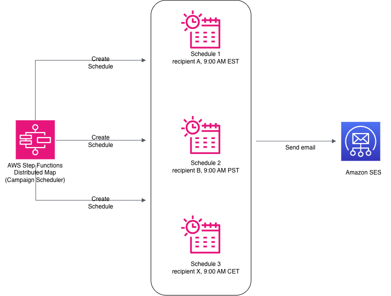
The architecture follows an event-driven, per-recipient scheduling pattern for an email campaign. To start the campaign, you first define the target audience and the content they receive. Next, you need a way to create the per-recipient schedule. To do that for a campaign that can contain millions of recipients, you need a scalable mechanism to create the schedules. You can achieve this with an AWS Step Functions state machine, a serverless workflow service that coordinates multiple AWS services into structured, visual workflows called state machines. In this solution, we orchestrate the creation of the schedules by using a Distributed Map state within the state machine, which lets us fan out and accelerate schedule creation. It does this by splitting a large dataset into chunks and processing them across thousands of parallel child executions. It reads the recipient list from Amazon Simple Storage Service (Amazon S3), applies time zone logic per recipient, and creates an individual Amazon EventBridge Scheduler resource for each recipient in parallel. After the workflow creates all schedules, the execution completes.
The actual email delivery happens later, entirely decoupled from the campaign creation step. At the scheduled time, Amazon EventBridge Scheduler invokes Amazon Simple Email Service (Amazon SES) directly, passing the template name and personalization data as template variables. For campaigns requiring complex personalization logic (conditional content, real-time suppression checks, or data enrichment), you can optionally route through an AWS Lambda function before SES. If you need to adjust timing or content for specific recipients, you can update their individual schedules directly without reprocessing the entire campaign.
Figure 1: Per-recipient email scheduling architecture with Amazon EventBridge Scheduler
Walkthrough
The solution uses four core components that work together: a campaign manager to define send-time rules, Step Functions Distributed Map to fan out and accelerate schedule creation, Amazon EventBridge Scheduler to hold each per-recipient intent and deliver through Amazon SES directly, and automatic cleanup through schedule self-deletion.
How it works
Create the campaign: A marketer defines the campaign: audience segment, email template, and send-time rules (for example, “9 AM in each recipient’s local time zone” or “24 hours before a Black Friday sale”).
Campaign manager fans out: An AWS Step Functions workflow uses Distributed Map to iterate over the recipient list and create one Amazon EventBridge Scheduler schedule per recipient per campaign step directly through SDK integration. Each schedule encodes the exact send time for that individual.
Amazon EventBridge Scheduler fires at the right moment: At each recipient’s scheduled time, Amazon EventBridge Scheduler invokes Amazon SES directly through a universal target, passing the template name and personalization data (recipient name and attributes) as template variables.
SES personalizes and sends: Amazon SES renders the email template with the provided data and delivers the message.
Schedule self-deletes: ActionAfterCompletion='DELETE' prevents the accumulation of spent schedules.
Prerequisites
To follow along with this walkthrough, you need the following:
AWS account and permissions: An active AWS account with permissions to create Amazon EventBridge Scheduler schedules, AWS Step Functions state machines, and Amazon SES identities, along with an AWS Identity and Access Management (IAM) role for Amazon EventBridge Scheduler to invoke Amazon SES.
Development environment: Python 3.13 or later, AWS SDK for Python (Boto3) version 1.26 or later, and AWS Command Line Interface v2 (AWS CLI v2).
Amazon SES configuration: Move your Amazon SES account out of sandbox mode to allow sending to arbitrary recipients.
Scaling the fan-out with Step Functions
For campaigns with millions of recipients, use AWS Step Functions Distributed Map to parallelize schedule creation. When you want to activate a campaign, you trigger a Step Functions workflow. This workflow fans out and creates schedules across the recipient list by using a Distributed Map with direct SDK integration. The direct SDK integration between Step Functions and Amazon EventBridge Scheduler lets each child execution call CreateSchedule directly. The following state machine definition reads recipients from an Amazon S3 CSV file and creates schedules in parallel:
Concurrency alignment with Amazon EventBridge Scheduler API limits
Step Functions Distributed Map supports up to 10,000 concurrent child workflows. Each child calls the CreateSchedule API directly, which has a default rate limit of 5,000 TPS. This limit is sufficient for most campaigns. If your campaign volumes require higher throughput, check your current quotas in the Service Quotas console and request an increase.
To avoid throttling, set MaxConcurrency below the CreateSchedule TPS quota. A value of 2,500 provides a comfortable buffer to account for bursts and retries without requiring a quota change. For larger campaigns, request an increase through AWS Service Quotas (adjustable to tens of thousands) and raise MaxConcurrency to match.
Canceling a campaign
A schedule group is an Amazon EventBridge Scheduler resource used to organize schedules. For this use case, we have a schedule group per campaign. If you need to pull a campaign (error in content, legal issue, or strategy change), you can cancel all scheduled sends for that campaign by deleting the entire schedule group. The following code shows how to cancel all pending sends for a campaign:
def cancel_campaign(campaign_id):
    """Cancel all pending sends for a campaign by deleting its schedule group."""
    scheduler.delete_schedule_group(
        Name=f'campaign-{campaign_id}'
    )
Operational considerations
Moving to production introduces a few scaling and reliability concerns to plan for.
Handling invocation spikes at delivery time
When a mass campaign schedules millions of messages for the same time, this creates cascading pressure across two limits:
Amazon EventBridge Scheduler invocations throttle limit: The default is 1,000 TPS per AWS Region, and it is adjustable to tens of thousands of TPS through AWS Service Quotas. Amazon EventBridge Scheduler queues invocations internally and retries with exponential backoff when the downstream target throttles.
Amazon SES sending quotas: Your SES account has a per-second sending rate. If the effective invocation rate exceeds this, messages fail with throttling errors. Align Amazon SES sending quotas with your campaign volume. Check your current SES quota in the Service Quotas console and request an increase before launching large campaigns. See Amazon SES best practices for deliverability at scale.
To handle an invocation spike, we recommend using the FlexibleTimeWindow feature of Amazon EventBridge Scheduler. Setting MaximumWindowInMinutes lets Amazon EventBridge Scheduler spread invocations across a time window rather than firing them all at the exact second. Size the window based on your campaign: divide the total schedules by your effective TPS to determine the minimum spread needed. For example, 500,000 schedules at 5,000 TPS need at least a 2-minute window.
Cost model
You pay for Amazon EventBridge Scheduler on a per-invocation basis.
Cleanup
To avoid ongoing charges, delete the resources created during this walkthrough:
Note: If you have active schedules still waiting to fire, deleting the schedule group will cancel all pending sends.
IAM role for Amazon EventBridge Scheduler and Step Functions
The Step Functions state machine needs an execution role with permissions to create schedules, send email, and pass the role to the Amazon EventBridge Scheduler service. Amazon EventBridge Scheduler needs permissions to call SES. The following policy shows the combined permissions for both scenarios:
This policy scopes the scheduler:CreateSchedule and scheduler:CreateScheduleGroup actions to resources prefixed with campaign-*, following least-privilege principles.
A condition restricts the iam:PassRole permission so that it can only pass the role to the Amazon EventBridge Scheduler service.
Conclusion
In this post, we walked through how to use Amazon EventBridge Scheduler to personalize email campaign delivery for each recipient. An email campaign system has two core problems: deciding what to send and deciding when to send it. Most teams over-engineer the “when” with polling infrastructure, batch jobs, and queue chains. Amazon EventBridge Scheduler collapses that into a single CreateSchedule API call per recipient.
Memory costs are increasing dramatically. Both RAM and hard disk drive prices have exploded over the past year. At Cloudflare, we run several massively distributed storage products (including our famous CDN) that rely on making efficient use of the memory we have deployed so we can continue to serve all of our customers.
With this in mind, we prototyped a way to expand effective cache capacity. By encoding eligible assets with Zstandard inside Pingora, the architecture trades a minor CPU increase for significant storage and cross-data center bandwidth savings.
We have been prototyping a system called Cache Transcoding, which I built during my internship at Cloudflare as part of the 1.1.1.1 Intern Program. When an eligible response enters the cache, we encode it using Zstandard, or zstd, before writing it to disk. We keep that compressed form while the asset lives in the cache and moves between data centers via Tiered Cache, then decode it before serving the response to the client.
In our initial testing, this encoding shrunk eligible assets to ⅓ of their original on-disk size on average. The estimated extra CPU cost in our origin-facing proxy was small, but that is the trade. A small increase in CPU gives Cloudflare petabytes of effective cache capacity and reduces the data transferred between our data centers. The encoding cost is paid once when an asset enters the cache. The storage and bandwidth savings continue every single time that asset is reused.
What is Zstandard?
Zstandard, or zstd, is a lossless compression algorithm developed by Yann Collet at Facebook and open sourced in 2016. Lossless means that after compressed data is decoded, every byte is identical to the original. We can change how an asset is represented on disk without changing the asset itself.
Zstd is designed to balance compression ratio with speed. In our earlier browser compression testing, it compressed data 42% faster than Brotli while producing nearly the same file size, and produced files 11.3% smaller than gzip at a comparable speed. That balance matters because Cache Transcoding would touch a large amount of traffic, so both encoding and decoding need to stay fast.
The prototype uses zstd level 3, giving us most of the compression benefit without turning cache fills into a CPU bottleneck.
Cloudflare traditionally stores an asset using the content encoding supplied by its origin. If an origin sends an uncompressed response, we store those uncompressed bytes on disk and transfer them between data centers in the same form. Cache Transcoding adds compression inside the cache itself.
Not everything is worth compressing
Transcoding does not mean compressing everything. Images, video, and fonts are usually compressed already. In our traffic sample, this media slice represented 21.4% of requests but 63.3% of bytes. Compressing it again would burn CPU for nothing.
Compressible text is different. HTML, JSON, CSS, and JavaScript represented 67.3% of requests and 22.3% of bytes. Within that text slice, approximately 71% arrived uncompressed with Content-Encoding unset and it compresses well.
In our controlled test corpus, the eligible assets compressed by roughly 2.8 times.
Encoding is more expensive per byte, but assets are served far more often than they are filled.
By changing how assets are represented, existing hardware could store more customer content.
Fewer bytes on disk mean each server can retain more objects. This increases cache density and reduces the likelihood that useful content is evicted because an uncompressed representation consumed more space than necessary.
The smaller representation also helps as an asset moves through Tiered Cache because it reduces the data transferred between Cloudflare data centers, making backbone usage more efficient.
Paying the compression cost once
Compression is never free. Encoding and decoding both use CPU, so the important question is whether the byte savings are worth the processing cost.
At zstd level 3 (often the default balance of speed and compression size output), our model kept the extra CPU cost to a few percent under the traffic and reuse assumptions we tested.
We initially considered limiting transcoding to popular content, since hot assets are reused more, but it did not help. Decoding happens every time an asset is served, so limiting the feature to only the hottest content reduced the storage saving without cutting CPU by the same amount.
The simpler policy performed better. Transcoding all eligible compressible text at or above 4 kibibytes (KiB) captured nearly all of the measured storage benefit, while remaining within the CPU budget.
How Cache Transcoding works
On a cache miss, our Pingora-based proxy encodes the body using zstd before writing it to disk. The cache metadata records that the stored representation is compressed and preserves the original content length. Before the response leaves the proxy, the body is decoded back to its original identity representation.
On a cache hit, the stored zstd object is read from disk and decoded. With Tiered Cache, the compressed representation is transferred from the upper tier to the lower tier in the compressed form. Decoding only happens on the client-facing hop.
On a full cache miss, the upper tier fetches identity bytes from the origin. Those bytes are encoded once, stored as zstd, and transferred to the lower tier in their compressed form. The lower tier also stores the zstd representation, then decodes it for the request path.
If the lower tier misses but the upper tier already has the object, the origin is not involved. The compressed object moves directly between the cache tiers. It remains compressed on the wire and on disk, then is decoded once at the lower tier.
If the lower tier already has the object, no network transfer or encoding is needed. The lower tier reads the zstd bytes from disk, decodes them, and passes the original asset onward.
The storage encoding marker prevents an object from being encoded more than once. A cache layer receiving an object from another tier can see that it is already stored using zstd, and preserve it in that form.
Why we only transcode certain text
The fastest compression operation is the one we do not need to perform. Cache Transcoding therefore uses a series of eligibility checks to avoid content that is unlikely to benefit.
The prototype only transcodes a 200 OK response when Content-Encoding is unset, the Content-Type is compressible text, and the response has a known Content-Length of at least 4 KiB. Slice subrequests, responses using active upstream compression, range requests, precompressed responses, unknown length bodies, and binary content remain unchanged.
The 4 KiB threshold removed a large number of tiny requests while leaving out only about 1% of the otherwise eligible bytes. Lowering it would add per-object overhead without saving much more storage.
The threshold and zstd level are both parameters rather than permanent limits. We started with zstd level 3 and a 4 KiB minimum because they gave us a conservative way to measure the architecture. With the initial CPU budget understood, we can test whether higher compression levels improve the ratio enough to justify their additional cost.
Testing over one million requests through the cache
We exercised the prototype against a controlled test zone and correlated each request across request logs, Prometheus metrics, and Jaeger traces.
The correctness campaign covered cache misses, cache hits, single-hop fills, Tiered Cache fills, and more. We varied cache keys to make each request follow a specific path and used traces to confirm where encoding and decoding occurred.
One performance campaign sent more than a million requests across 10 cache servers. Half of the campaign ran with Tiered Cache disabled and the other half with it enabled. This allowed us to measure local cache behavior separately from transfers between cache tiers.
The two assets were approximately 195 KiB and 272 KiB, and both compressed by roughly 2.8 times. This was deliberately a compressible test corpus. It gave us a clear signal for validating the architecture, but it does not represent every text object on the Internet. A broader corpus is required before treating the measured compression ratio as a fleet-wide constant.
Compress once, benefit many times
What this experiment showed us is that there are significant efficiencies we can still deploy across our caching service that can benefit all of our customers. What we built for Cache Transcoding shows that the trade is favorable under the conditions we tested. The architecture preserved the content and remained within the CPU budget.
For next steps, we plan to evaluate higher zstd levels, test a broader range of content types and object sizes, tune different parameters from the eligibility criteria and more. Future work can also examine range requests, pre-compressed origin responses, and passing the compressed object directly to downstream components that already support it without decoding.
Throughout my internship, I’ve had the wonderful opportunity to work alongside Cloudflare's engineering teams on the real infrastructure that stores and serves content across our global network. If you want to start your career by helping build a better Internet, explore our internship opportunities and job openings.
Nathan E. Sanders and I are writing a series of essays on real-world examples of democratic technologies for The Renovator. I haven’t been posting the full text on the blog because they’re a bit long, but here are links.
Part 1 is about the Japanese digital democracy party, Team Mirai.
Part 2 is about the Swiss Public AI model, Apertus.
Part 3 is about the civic technologists of Open Knowledge Brazil.
And the new one, Part 4, is about civic AI in Scotland.
На 25-ти октомври 2026 ще се проведат избори за президент и вицепрезидент. Ето най-важното към този момент.
Все още не е публикуван електронният формуляр за заявление за гласуване. Очакваме го до 11-ти септември, когато ще ви изпратя допълнителен мейл на абониралите се с нужната информация. Разбираме от хронограмата на ЦИК, че срокът на подаване е 29-ти септември. В последните 10 години времето за подаване на заявления варира от 17 дни на изборите през 2023-та до 28 дни през октомври 2024 и април 2021-ва. Както и на предишни избори, събирането на заявления ще се следи в реално време на карта на Glasuvam.org.
През 2026 г. бяха приети редица промени в Изборния кодекс. Преди парламентарните избори в началото на годината беше въведено ограничаване на броя секции в държави извън Европейския съюз. Как се стигна до това предложение и кои депутати гласуваха за него ще намерите обобщено в тези данни и на записа на дебатите в зала. Обобщил съм ги в тази статия. След изборите това ограничение отпадна, но остана правилото, че извън ЕС ще могат да се отварят секции само при 40 подадени заявления и по преценка на дипломатическите представителства. Това означава, че подаването на заявление е още по-важно от предходни години.
В следващите три дни – до 4-ти септември – трябва да бъдат обявени местата в чужбина, където в последните пет години е имало поне 100 гласували. Това ще включва 5-те вота от 25 октомври 2021-ва до сега. Изключва последните президентски изори, които се проведоха на 21-ви октомври. Отделно някои държави като Германия трябва изрично да дадат съгласие за досегашните места. Тук подаването на заявления отново ще е от значение, защото от една страна ще даде сведение на МВнР за местата, където има интерес, а от друга – ще бъде повод да се отварят повече секции на едно и също място предвид повишения интерес.
Важно е да се отбележи, че подаването на заявления не е задължително. Може да гласувате където и да е по света дори да не сте подали заявление или да не живеете постоянно в чужбина. Може да гласувате на което и да е място дори да сте подали заявление за друго. Заявленията обаче са критични за възможността Ви да упражните гласа си, както и за по-бързото провеждане на изборния ден.
Както стана видно в последните няколко вота, проблем с провеждането на изборите има, особено що се отнася до гладкото провеждане на изборния ден, надеждността на броенето, предотвратяване на злоупотреби и грешки. Затова, ако имате възможност, ви призовавам да се присъедините към секционните комисии или като доброволци. За целта се свържете с най-близкото до вас посолство като изявите това желание. Алтернативно, може да се присъедините като доброволец към инициативата ТиБроиш за следене честността на вота. Дори от дистанция може да участвате като следите излъчванията от секции в цяла България и да пренасяте данните от сниманите протоколи. В последните години много злоупотреби станали вече емблематични са били засечени именно по този начин. Може да се запишете тук и ще се свържат с вас за повече подробности.
Повече информация ще намерите на сайта на ЦИК, МВнР, както и в следващите статии в блога ми. Условията и редът за създаване на секции, провеждане на изборния ден и незабавните задачи пред посолствата и МВнР ще намерите в решението на ЦИК от 27-ми август.
Amazon Kinesis Data Streams now supports streaming tables, a fully managed capability that continuously delivers your streaming data as queryable Apache Iceberg tables on Amazon S3 Tables. Amazon S3 Tables is a capability of Amazon Simple Storage Service (Amazon S3). Streaming tables reduce data delivery costs to S3 Tables by up to 50% compared to self-managed alternatives and reduce downstream query costs by up to 30% through intelligent inline compaction that eliminates the small file problem. You need no custom applications, no self-managed compute, and no operational overhead.
Customers increasingly want to unify streaming data with Apache Iceberg for near-real-time analytics, fraud detection, personalization, and artificial intelligence and machine learning (AI/ML) feature pipelines. But integrating the two has meant operating complex custom connectors, managing format conversions, and contending with the performance impact of many small Parquet files that slow queries and increase costs. Streaming tables solve this: configure delivery in a few steps from the console or through APIs, and your data becomes queryable from Amazon Athena, Amazon Redshift, and Apache Spark within minutes. Tables are automatically registered in AWS Glue Data Catalog, making them immediately discoverable for analytics engines and AI agents.
For workloads that don’t require Iceberg table format, you can also deliver streaming data to Amazon S3 general purpose buckets. Delivery is in the source data format, ideal for archival, backup, and ML training data pipelines, with the same serverless, fully managed delivery and no infrastructure to operate.
Challenges with delivering streaming data to Apache Iceberg
Customers today face three challenges when integrating streaming data with Apache Iceberg.
Operational complexity: Connecting Kinesis Data Streams to Iceberg tables today requires deploying and maintaining custom connectors, Apache Flink jobs, or consumer applications. Teams must manage pipeline failures, handle format conversions, scale infrastructure, and monitor delivery reliability. These operational tasks consume significant engineering time and introduce ongoing risk of downtime.
Resiliency and the small file problem: Without proper coordination, simultaneous writes from multiple high-throughput shards can conflict, leading to failed commits, data freshness delays, and degraded performance. Streaming ingestion of high-volume data creates large numbers of small Parquet files in Iceberg tables, forcing a difficult trade-off between data freshness and query efficiency.
Cost: Customers typically spend up to $28/TB operating streaming extract, transform, and load (ETL) pipelines from Kinesis Data Streams using self-managed alternatives based on internal analysis. This creates a high price barrier to getting streaming data into queryable formats and makes cost unpredictable as volume grows.
How delivery to streaming tables solves these challenges
Streaming tables are a native capability built directly into Amazon Kinesis Data Streams. There is no separate service to deploy, no connector to version, and no consumer application to maintain. You enable delivery in a few steps from the console or through APIs.
Zero operational overhead: Streaming tables remove the need to build and operate custom consumer applications for data delivery. No pipeline infrastructure to provision, no scaling logic to write, no failure handling to implement. The capability automatically scales to process gigabytes per second of throughput.
Built-in resiliency: Streaming tables provide write coordination and exactly once delivery semantics across all shards in your stream, resolving concurrent writer conflicts and ensuring data integrity without manual intervention.
Intelligent compaction, no trade-offs: During ingestion, streaming tables perform inline compaction that produces query-optimized Parquet files, eliminating the small file problem while maintaining minute-level data freshness. This reduces downstream query costs by up to 30 percent compared to uncompacted delivery.
Consumption-based pricing: You pay only for data delivered: $14/TB for Iceberg delivery to S3 Tables in US East (N. Virginia) Region (us-east-1) (50% savings compared to self-managed alternatives) and $11/TB for general purpose S3 delivery (60% savings compared to self-managed alternatives). When your stream is idle, you pay nothing for delivery. Combined with Kinesis Data Streams On-Demand Advantage pricing, which eliminates per-shard charges and scales automatically, the entire path from ingestion to queryable Iceberg tables operates on a pure consumption model.
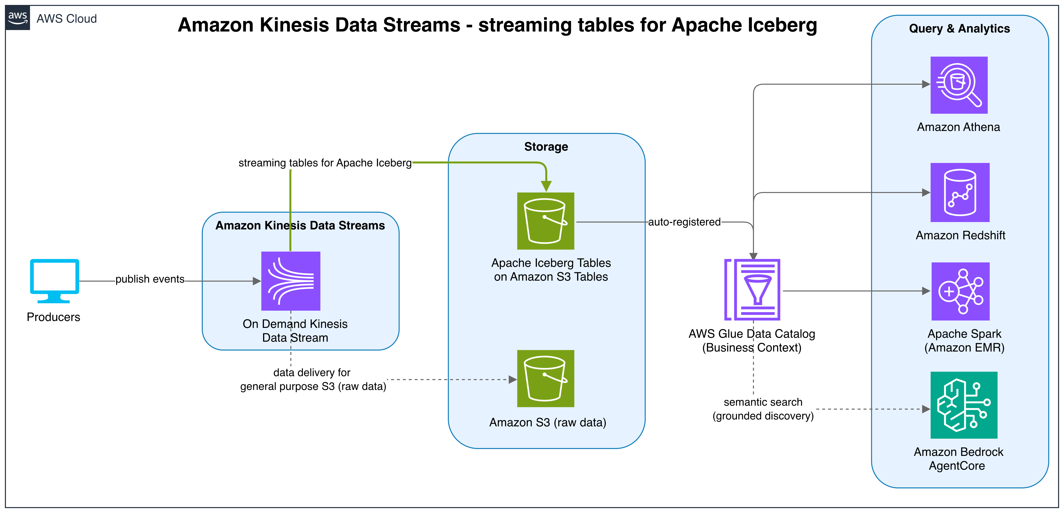
With delivery to streaming tables, you now have a fully managed end-to-end real-time data architecture from data ingestion through storage to analytics. Your producers publish events to a Kinesis Data Stream, which continuously delivers data as optimized Iceberg read-only tables in S3 Tables. From there, you can query your streaming data using analytics engines like Amazon Athena, Amazon Redshift, Amazon EMR (Apache Spark), or Apache Flink. You can also let AI agents discover and reason over your data through Glue Data Catalog semantic search. This managed experience removes the intermediate infrastructure that customers previously assembled: separate connector clusters, compaction jobs, and custom consumers. It replaces them with a single, serverless pipeline from stream to insight.
The following diagram illustrates this end-to-end architecture.
Figure 1: End-to-end managed streaming analytics architecture from ingestion to query
Getting started
To get started, sign in to the Amazon Kinesis Data Streams console, navigate to your streams, and enable delivery to streaming tables in a few steps. Specify the stream you want to deliver, configure your schema settings using AWS Glue Schema Registry, and choose your destination S3 Tables location. After you enable it, delivery to streaming tables immediately begins materializing your streaming data as queryable Iceberg tables in S3 with no further intervention required. There’s no infrastructure to provision and no minimum commitment. You pay only for data delivered.
Additionally, you can use Amazon Kinesis Data Streams APIs to programmatically set up, update, or delete delivery to streaming tables configurations for your data streams. With these APIs, teams can build agentic workflows and infrastructure-as-code patterns to manage configurations across multiple data streams at scale.
Getting started with the Kinesis Data Streams Agent Skill
The Kinesis Data Streams Agent Skill provides AI-assisted guidance for setting up streaming tables integrations for your existing or new data streams. The skill helps you configure delivery to S3 Tables (Iceberg) or S3, including schema registry setup, AWS Identity and Access Management (IAM) role configuration, and validation.
Installing as an Agent Skill
Agent Skills are discovered automatically by compatible tools through the SKILL.md file. Refer to the Agent Toolkit for AWS Skill Installation Guide to install the managing-amazon-kinesis-data-streams Agent Skill. We also recommend you install the AWS MCP Server in your developer tool of choice, which exposes tools for searching AWS documentation, blogs, and Skills dynamically at runtime. These capabilities make agents more accurate and powerful for AWS related development and operational tasks, and make skill discovery and installation more flexible. Refer to Setting up the AWS MCP Server for guidance on installing the AWS MCP Server in your environment.
To verify the installation, interact with the skill in your preferred tool.
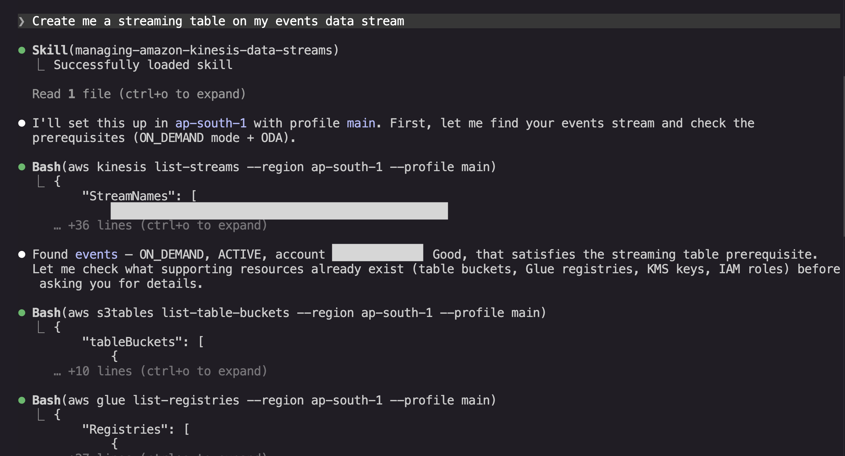
To start delivering data from your data streams to Apache Iceberg tables in real time, prompt “Create me a streaming table on my events data stream” to your agent of choice:
Figure 2: Prompting the agent to create a streaming table
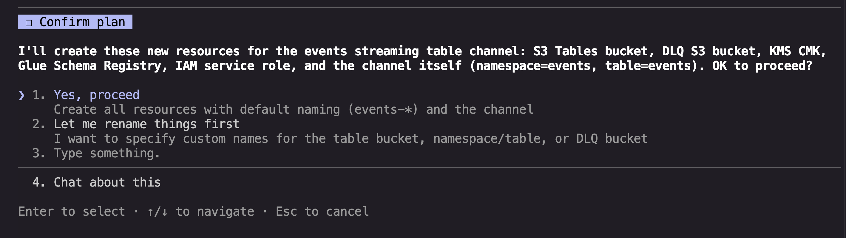
The agent dynamically loads the managing-amazon-kinesis-data-streams skill and starts by gathering the available resources in your AWS account for the streaming tables integration. After it gathers that data, it confirms the resources to use or create, and creates the integration:
Figure 3: The agent confirming resources before creating the integration
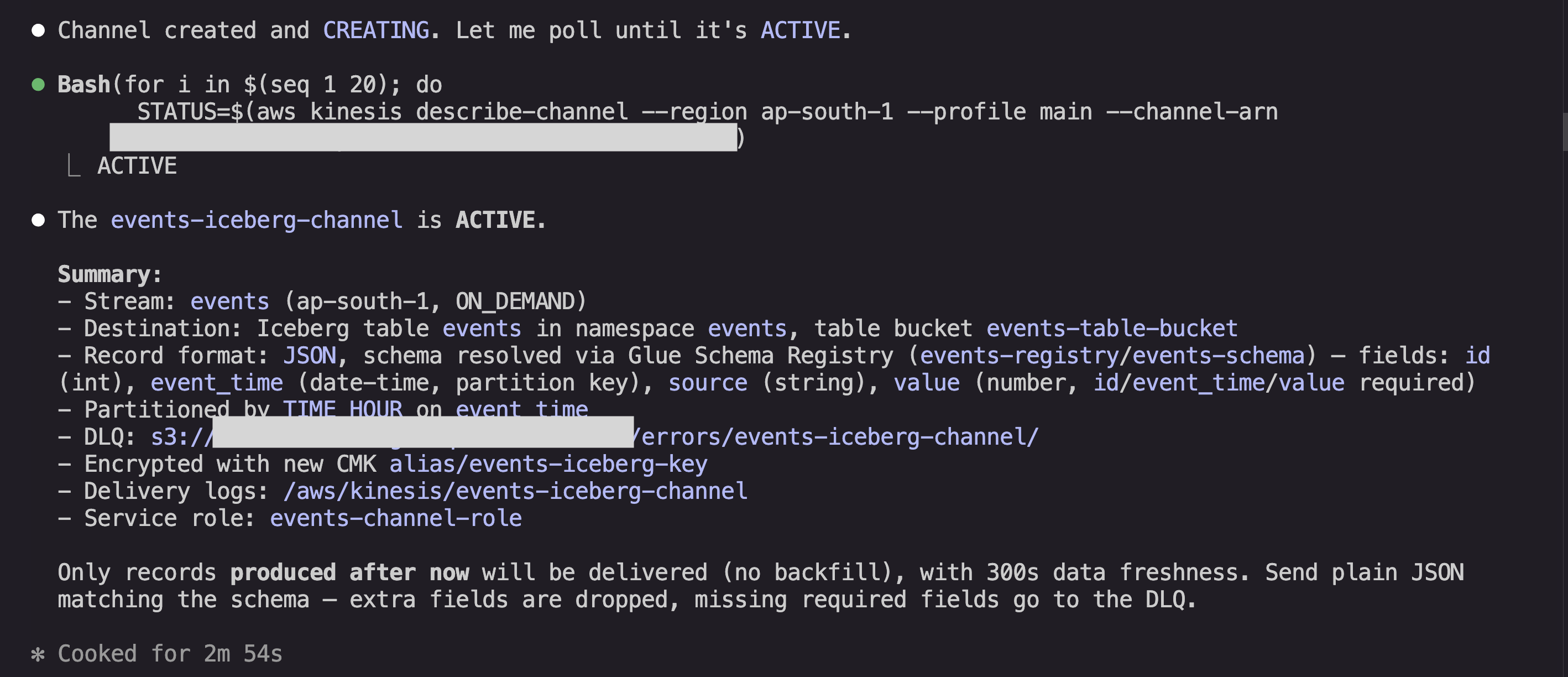
After creating the integration, the agent summarizes the status and can then help with any other operational tasks with your data. For example, the agent can help you set up AWS Lake Formation permissions to query the data in S3 Tables with Athena, or configure your table maintenance behavior in S3 Tables:
Figure 4: The agent offering follow-up operational tasks
Conclusion
Streaming tables are available in all AWS Regions where Amazon Kinesis Data Streams is offered. Pricing is $14/TB for delivery to S3 Tables (Apache Iceberg) and $11/TB for delivery to general purpose S3 buckets. To learn more, visit the documentation and pricing pages.
Search is the front door of many applications, yet most teams struggle to answer a deceptively simple question: “Is my search actually returning relevant results?” Query logs tell you what users typed, not what they saw, what they selected, or why they left. When search feels broken, the culprit is rarely the engine. It’s the lack of deliberate signal collection, measurement, and a feedback loop to act on it.
You can close this gap on Amazon OpenSearch Service using User Behavior Insights (UBI), an open schema standard for capturing search behavior, and Search Relevance Workbench (SRW), a toolkit for measuring and evaluating search quality. Your application generates the UBI-formatted records. Together, UBI and SRW give you a repeatable framework: collect signals, turn them into relevance judgments, and validate every change before it ships.
In this post, we show you how to capture UBI data on an Amazon OpenSearch Service domain and use those signals to evaluate search quality. This is the first post in a two-part series. We build the foundation here, and Part 2 covers automating the workflow end to end.
The challenge: You can’t improve what you can’t measure
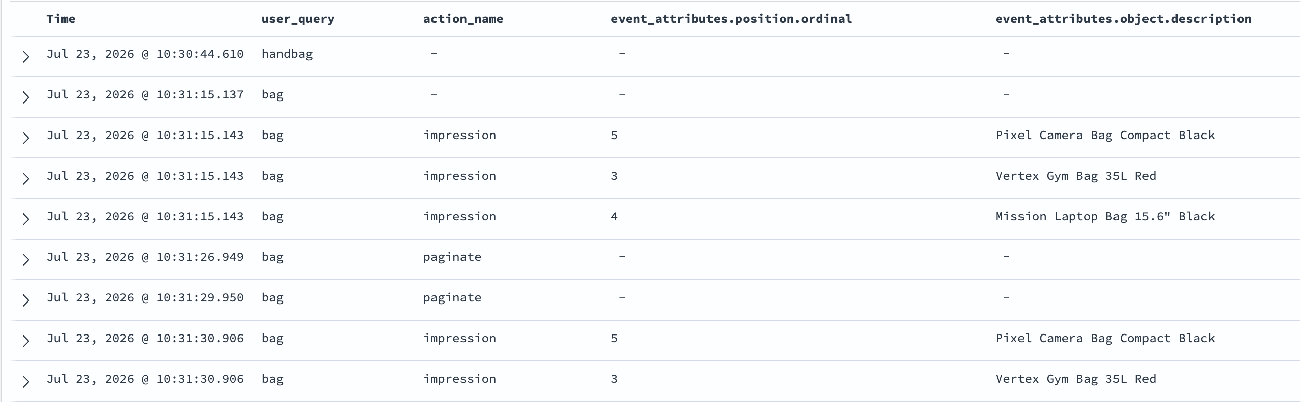
Consider a shopper searching for “handbag” on an ecommerce site. The catalog has 16 products (tote bags, duffel bags, laptop bags), but every title only says “bag.” The search returns zero results. Most shoppers leave. A patient one retries with “bag” and finds what they were looking for.
Your server log recorded that first query as a clean sub-second response: no error, no alert, no signal. What it missed entirely was a customer with purchase intent. That customer hit a vocabulary gap between how they search and how you write your catalog. Zoom out and apply this lens to misspelled queries, poor handling of long-tail searches, and abandoned sessions. The blind spot is larger than you think.
There’s a second problem: click signals are position biased. Users select the first result far more than the fifth, regardless of relevance, so raw click counts reflect where results appeared, not whether they deserved to be there. Any judgment derived from clicks must correct for this bias. We return to it when generating judgments.
Capturing behavioral data with UBI
UBI defines two indices. The ubi_queries index holds one record per executed query: the text the user typed, the full query that ran (filters and facets included), and the IDs of the documents returned. The ubi_events index holds every subsequent user action: impressions, hovers, clicks, add-to-carts, each stamped with the result position and the product’s business identifier (object_id). A shared query_id links every event back to the query that triggered it. Two additional identifiers complete the picture: client_id tracks the browser across visits, and session_id scopes events to a single visit.
A query record captures what the user asked and which document IDs the engine returned, including zero-result cases like the handbag search, which appears as a record with an empty result list. Here’s the shopper’s follow-up search for “bag”:
The event record captures what the user did next. For each result rendered, emit an impression event. When the user selects a result, emit a click event. Here is the impression event for the first result of the bag search:
event_attributes also accepts custom fields of your own alongside the standard position and object structures. The action_name attribute is critical: The judgment model you use later consumes only impression and click events. Treat a paginated results page as the same logical query: reuse the query_id and record absolute positions. The UBI events schema reference documents the complete event schema.
Collecting UBI data on Amazon OpenSearch Service
Behavioral data (what results ranked, what users saw, what they selected) exists only in the application layer. Your application owns the records, and Amazon OpenSearch Ingestion (OSI), a fully managed, serverless data collector powered by Data Prepper, provides the managed delivery path. Your application sends the records as SigV4-signed HTTP POST requests to the OSI pipeline endpoints. Route browser events through your backend for signing. One thing to understand before you write any code: Your application generates and owns the query_id attribute. The application creates the ID when it runs a search and stamps it on every subsequent event the user produces, until the user issues a new search or the session ends.
Prerequisites
To follow along, you need an Amazon OpenSearch Service domain running OpenSearch 3.5 or later with the OpenSearch UI application, permissions to create OpenSearch Ingestion pipelines with an AWS Identity and Access Management (IAM) pipeline role, and a search application you can instrument to emit behavioral records.
Create the UBI indices
Before you start collecting user metrics, you need the two indices in place with the right mappings. Field types matter here: query_id as keyword supports exact joins between queries and events, timestamp as date supports time-range queries, and event_attributes as dynamic means you can extend events with custom fields without schema changes.
Create ubi_queries first in Dev Tools. It holds the query-side records. We abbreviated the mappings here. Refer to the published queries-mapping.json file for the complete version:
With both indices created, the next step is routing data into them. You can deliver UBI data to your domain in several ways. This post uses OSI pipelines, shown end to end in the diagram that follows the setup.
Set up the OSI pipelines
Create two OSI pipelines: one for queries and another for events. Each pipeline exposes an HTTP source endpoint that your application writes to (shown on each pipeline’s console page) and sinks data to the corresponding index. The following configuration defines the events pipeline:
Note: the queries pipeline follows the same pattern, with /ubi/queries as the path and ubi_queries as the sink index and S3 prefix. Create the pipeline role yourself or let OpenSearch Ingestion create it. If your domain uses fine-grained access control, also map the pipeline role to a backend role so the domain accepts the pipeline’s writes. Refer to the tutorial Collecting UBI-formatted data in Amazon OpenSearch Service for detailed steps.
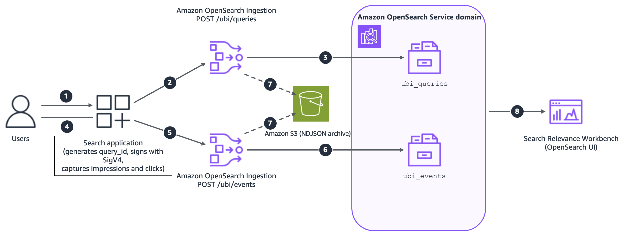
With the pipelines running, your application can start sending data. The following diagram illustrates the end-to-end flow:
Figure 1: The UBI collection pattern on Amazon OpenSearch Service
The workflow consists of the following steps:
Users interact with your search application.
The application sends signed query records to the OSI HTTP endpoint.
OSI writes queries to the ubi_queries index.
Users interact with the results, viewing and selecting documents.
The application sends signed event records, carrying the same query_id, to the OSI HTTP endpoint.
OSI writes events to the ubi_events index.
Optionally, both pipelines archive records to Amazon Simple Storage Service (Amazon S3).
Search Relevance Workbench (OpenSearch UI) works with the collected data in the ubi_queries and ubi_events indices.
Note: if you’re already collecting site analytics through an existing third-party tool, you don’t need to replace it. Map your search-related events (queries, clicks, and conversions) into the UBI schema and store them in OpenSearch. That’s enough to unlock the out-of-the-box evaluation framework, implicit judgment generation, and the full SRW metrics pipeline, without defining a single custom metric from scratch.
Visualize the data collected
After the UBI behavior metrics start to trickle in, you can review the data in the Discover tab on the OpenSearch UI dashboard. Filtering ubi_queries for empty result lists ranks your vocabulary gaps. You can also visualize the data collected through the sample User Behavior Insights (UBI) dashboards in OpenSearch.
Figure 2: UBI records in Discover, showing the zero-result handbag query and the follow-up bag query with its impressions and pagination events
With data flowing into your indices, keep these things in mind as you scale to production:
Keep telemetry off the search critical path – Queue records and forward them asynchronously. Losing a fraction of behavioral data is statistically harmless. Blocking users isn’t.
Manage volume deliberately – Batch impression events, and if you sample, sample whole queries rather than individual events to preserve the click-through ratios that drive judgments.
Isolate analytical load for larger deployments – Route pipelines to a separate analysis domain with the same engine version, mappings, and analyzers as production. This keeps behavioral writes from touching live search latency.
Plan for retention and integrity – Register the UBI mappings as an index template and apply an Index State Management (ISM) retention policy as your indices grow. You should validate and rate-limit the event write path, and cover query text and client identifiers with your data retention policy.
Evaluating search quality with Search Relevance Workbench
With ubi_queries and ubi_events collecting data, you now have the signals needed to evaluate search quality. Search Relevance Workbench, generally available in the OpenSearch UI from Amazon OpenSearch Service 3.5, turns those signals into structured experiments: comparing query configurations, scoring results against relevance judgments, and surfacing metrics that guide iterative tuning.
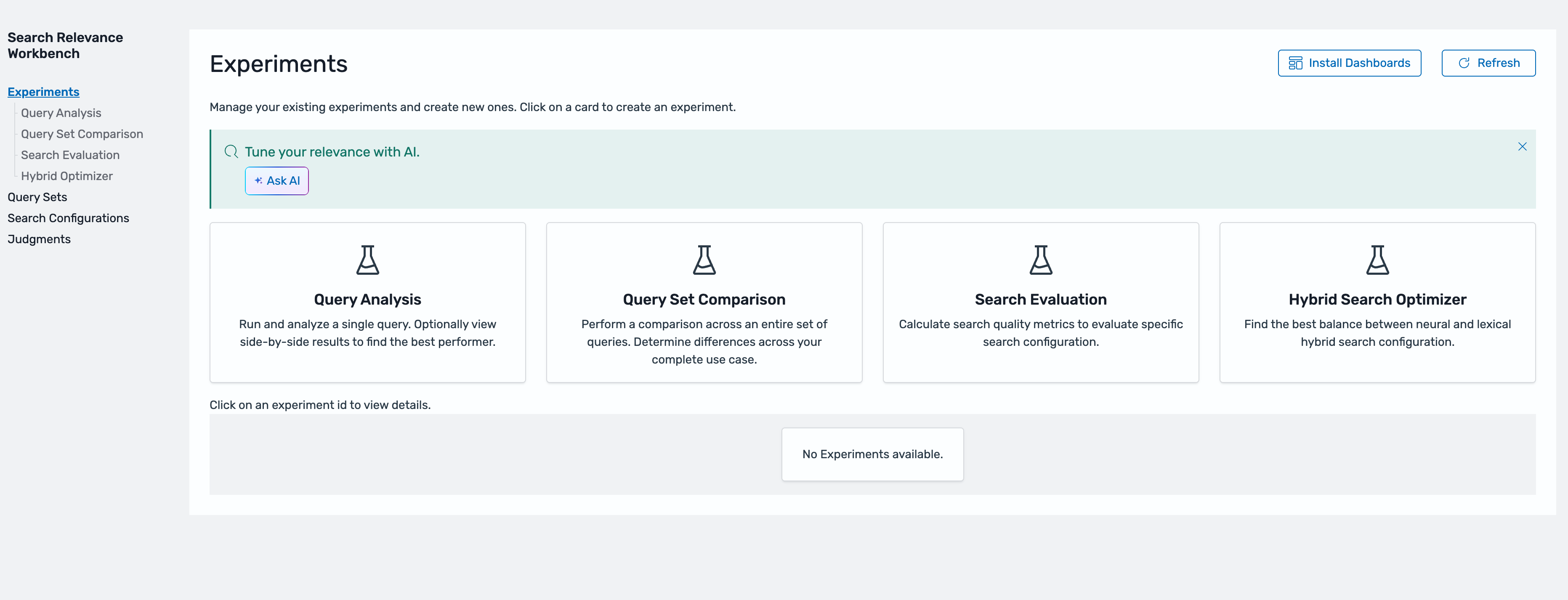
Figure 3: Search Relevance Workbench in the OpenSearch UI
SRW experiments rely on three components. You set them up once, then reuse them across every experiment you run: a query set (the fixed queries you evaluate against), search configurations (the query structures you want to compare), and a judgment list (the relevance ground truth). The following sections walk through each one.
Step 1: Create a query set
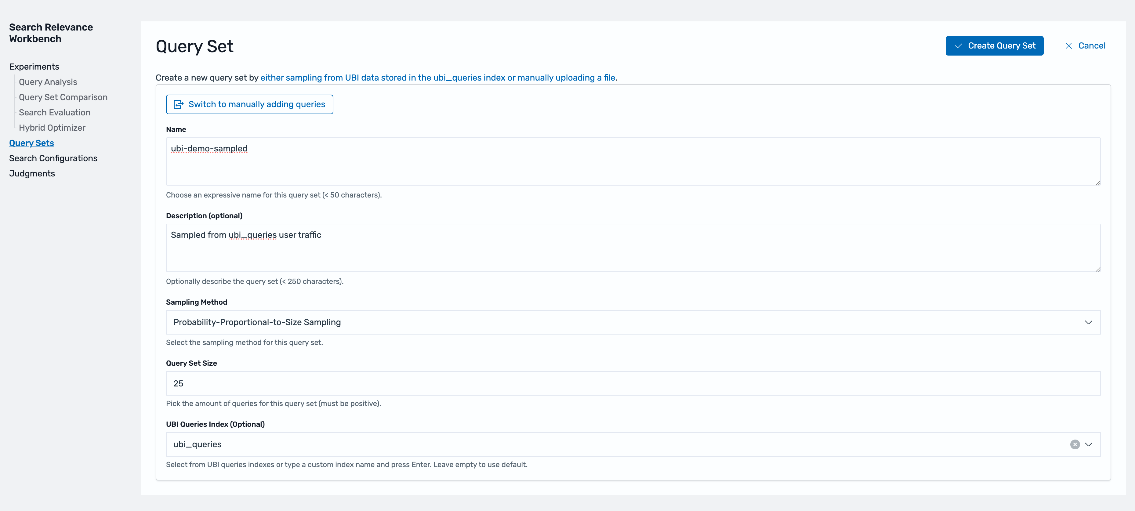
A query set is the fixed collection of queries you evaluate against. Keeping it fixed makes results comparable across experiments. Effective query sets reflect real traffic, not intuition. You can seed one from your top queries, a random sample, or a hand-picked mix that includes long-tail and low-performing queries. Alternatively, SRW can sample directly from ubi_queries using Probability-Proportional-to-Size (PPS) sampling, which selects queries in proportion to how often users issue them. This approach represents frequent queries like “bag”, so your metrics reflect search quality as users experience it.
Figure 4: Creating a query set sampled from real traffic in ubi_queries
Step 2: Define search configurations
A search configuration defines how a search executes: the index, the query structure, and a %SearchText% placeholder that SRW replaces with each query in your set. Creating two configurations and running them against the same query set and judgment list is how you validate a change before any user sees it.
As an example, here we define two configurations: a baseline multi_match query (retail_query) and a variant that boosts title matches (retail_boosted_query), so we can measure whether the boost actually helps ranking.
Configurations go beyond query variants: a candidate can be an entirely different retrieval strategy, like hybrid search combining keyword and neural retrieval. You can use judgments to rate query-document pairs independently of your retrieval approach. You can test a semantic or hybrid approach offline against your existing traffic before shipping it.
Step 3: Create the judgment list
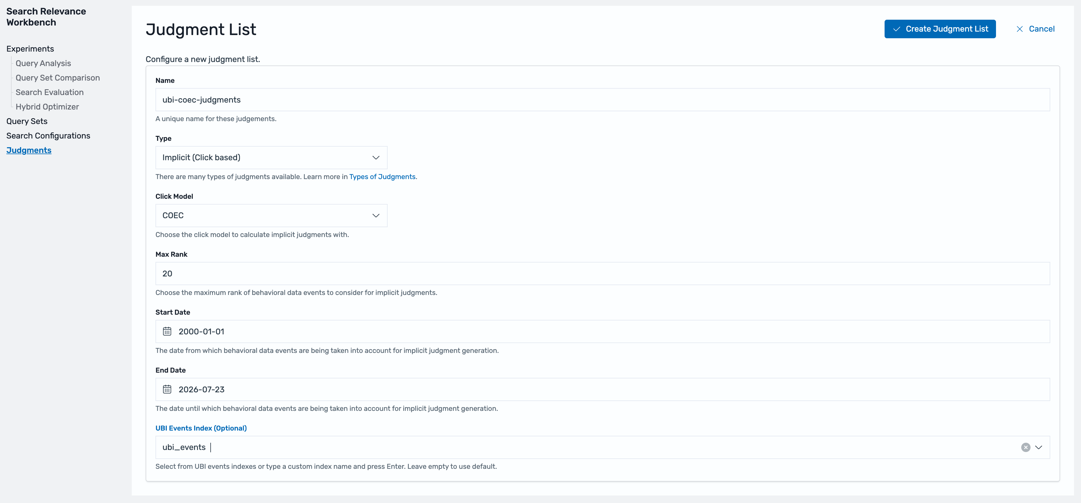
A judgment is a relevance rating for a query-document pair: the ground truth that quality metrics measure against. You can create judgments that are explicit (from stakeholders or a large language model acting as judge), imported, or implicit (derived from behavior). Here we use implicit judgments derived from UBI selection behavior, scored using the Clicks Over Expected Clicks (COEC) model. The COEC model helps correct position bias by comparing each document’s actual click rate against the expected rate for its rank position. Documents that outperform their position score as relevant. Those that users select because they ranked first score near average.
Figure 5: Creating an implicit judgment list with the Implicit (Click based) type and the COEC click model
Three things to get right before you run experiments:
object_id in your events must match the document _id from your product catalog. The search configurations you define return this _id, which lets SRW join judgments to results.
Implicit judgments are statistical. They need volume and query coverage. As a working rule of thumb, aim for hundreds to thousands of real sessions per query to separate signal from noise.
Max Rank controls how deep in the result list events count. If users paginate, set it beyond a single page. We use 20 here.
Step 4: Run experiments
This post uses three SRW capabilities: Query Analysis, Query Set Comparison, and Search Evaluation. Query Analysis is a quick eyeball check: compare two configurations side by side for a specific query to see exactly what changed and why the metrics moved. The other two answer harder questions with numbers: how good a configuration is, and how two configurations compare against real relevance signals.
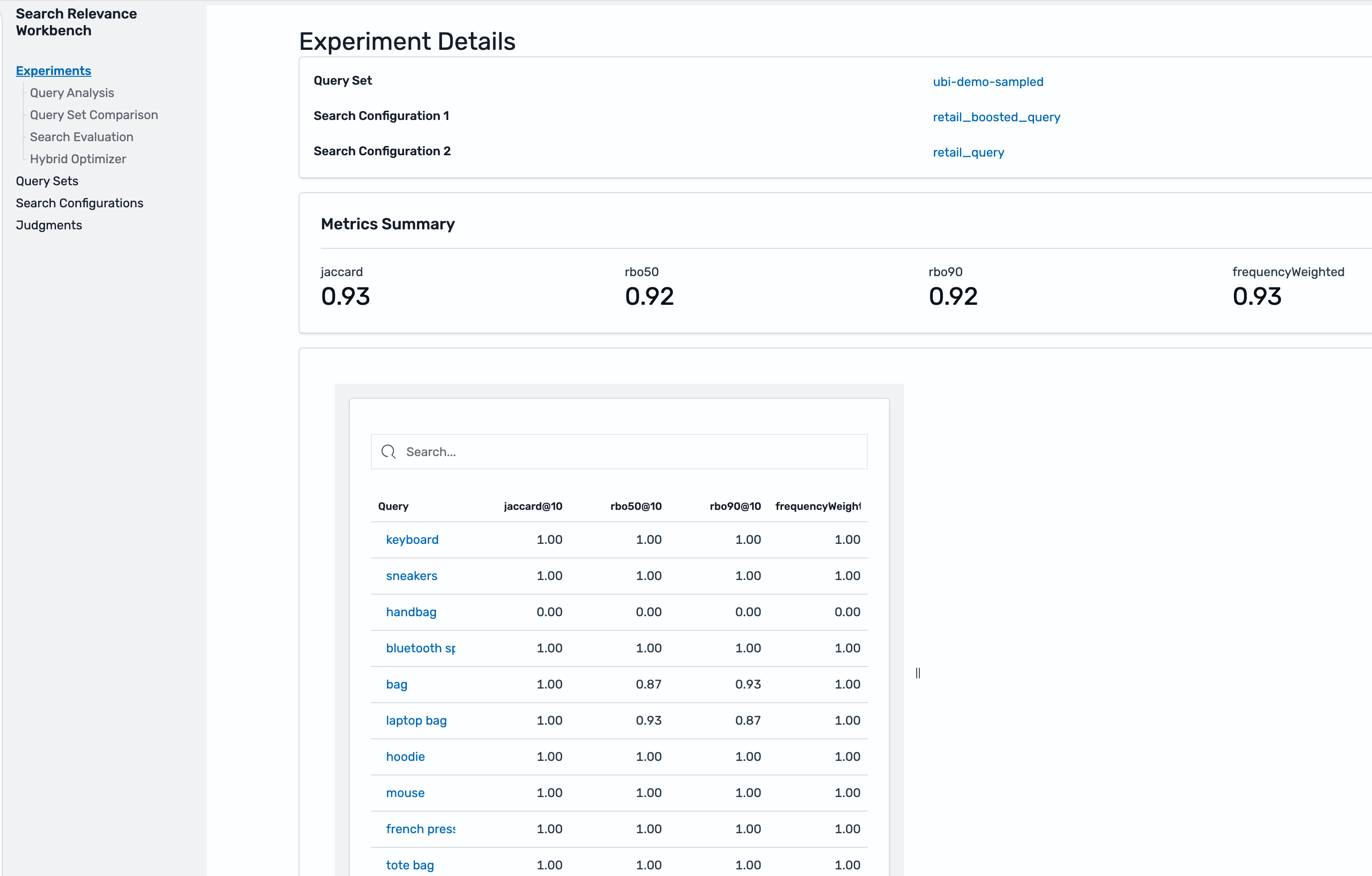
Query Set Comparison (also called pairwise comparison) takes two configurations and computes ranking similarity. Jaccard overlap measures how much the two result lists share, while Rank-Biased Overlap (RBO) weights agreement at the top of the list more heavily. Near-identical scores mean the change will barely register with users. Low overlap means a real ranking shift worth reviewing carefully before shipping. In this run, the two configurations score 0.93 Jaccard and 0.92 RBO, a modest but real shift. SRW cannot score zero-result queries like “handbag”: They show zero similarity in a comparison and Failed in an evaluation, a signal they need a different fix than ranking adjustments.
Figure 6: Query Set Comparison showing Jaccard and Rank-Biased Overlap between the two configurations
Search Evaluation (also called pointwise evaluation) scores one configuration against your query set and judgment list across four metrics, each computed over the top k results (k=10 by default):
Metric
What it measures
What it tells you
Coverage@k
Proportion of returned documents that have judgments
How much to trust the other three metrics. Low Coverage means many results were never judged
Precision@k
Fraction of the top k results that are relevant
How many irrelevant results appear on the first page
MAP@k (Mean Average Precision)
Precision averaged across ranks, rewarding relevant documents placed early
Whether relevant results appear early, even when Precision ties
NDCG@k (Normalized Discounted Cumulative Gain)
Graded judgment values, discounted by position (rank 1 counts more than rank 9)
Whether the best results appear first. The primary comparison metric
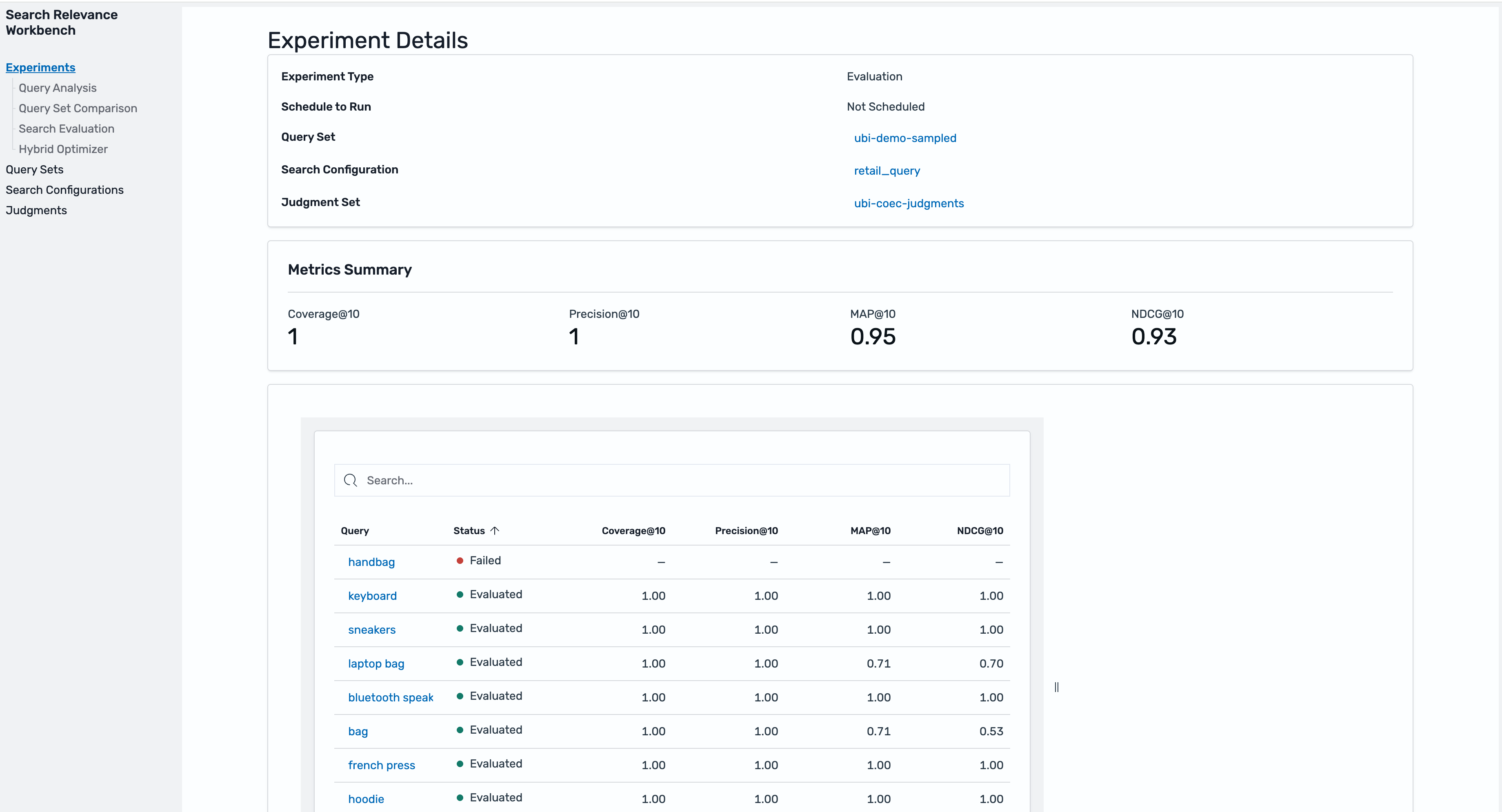
Each pointwise experiment evaluates one configuration. To compare candidates, run one experiment per configuration and compare the results. In this run, the baseline (retail_query) scores Coverage@10 of 1.0, Precision@10 of 1.0, MAP@10 of 0.95, and NDCG@10 of 0.93, with the zero-result “handbag” query showing as Failed in the per-query detail.
Figure 7: Search evaluation results for one configuration: Coverage, Precision, MAP, and NDCG at 10, with per-query detail
From measurement to improvement
The preceding experiments are the harness. The following are common levers to test with it. Express each as a new search configuration, evaluate it against the same query set and judgment list, and adopt it only if the metrics move:
Synonyms – One option for addressing known vocabulary gaps is to build synonyms. A search-time synonym token filter treats “handbag” and “bag” as equivalent, and with Amazon OpenSearch Service, you can hot deploy custom synonym packages without reindexing.
Field weights – Adjust the fields and boosts in a multi_match query, like the title^2 variant tested earlier.
Semantic retrieval – A hybrid query combines keyword and neural scores, addressing vocabulary mismatch as a class rather than term by term. Judgments evaluate it offline exactly like a lexical candidate.
Reranking – A rerank processor in a search pipeline reorders the top results using a cross-encoder model.
Clean up
To avoid future charges, delete the resources you created for this walkthrough:
If you configured the optional Amazon S3 archive, delete the archived objects (or the bucket).
If you keep the domain, optionally delete the ubi_queries and ubi_events indices and the query sets, judgment lists, and experiments you created. These live on the domain and incur no separate charges.
If you created the domain specifically for this post, delete it to remove everything, including the resources in the previous step. Deleting a domain is irreversible. Don’t delete a domain that serves other workloads.
Conclusion
UBI collects the evidence, COEC turns it into judgments, and SRW experiments deliver the verdict: Coverage, Precision, MAP, and NDCG in place of guesswork. Ship the winning configuration, keep collecting, and the next round of judgments shows whether the improvement holds with real behavior. Where there used to be an opinion, there is now a number.
Everything here follows a repeatable pattern, and repeatable patterns lend themselves to automation. Part 2 walks through the Search Relevance Agent, available through the AI Assistant chat (the Ask AI button) in the OpenSearch UI. The agent analyzes your UBI signals, generates tuning hypotheses, and validates them offline before recommending changes. The pipeline you built in this post is the foundation. Stay tuned for Part 2.
Today, Amazon EC2 R9g and R9gd instances are generally available, powered by AWS Graviton5 processors. R9g instances are memory-optimized and deliver up to 25% better compute performance compared to Graviton4-based R8g instances, powered by the most energy efficient processor AWS has ever built.
R9g instances are ideal for memory-intensive workloads including databases, in-memory caches (Valkey, Redis, MemCached), real-time big data analytics, Linux-based workloads including containerized and micro-service-based applications (e.g. Kubernetes, Docker, EKS, ECS), as well as applications written in popular programming languages such as C/C++, Rust, Go, Java, Python, .NET Core, Node.js, Ruby, and PHP.
R9gd instances include local NVMe-based SSD block-level storage, ideal for memory-intensive workloads requiring fast, low-latency local storage such as open-source databases, distributed real-time big data analytics, large in-memory databases, and large caching workloads.
If you’re running workloads on R8g instances today, R9g gives you more performance per vCPU with faster memory, higher network and Amazon EBS bandwidth, and a larger L3 cache, all while using less energy.
What makes R9g different Graviton5 processors bring several hardware improvements over Graviton4:
Up to 25% higher compute performance per vCPU
DDR5 8800 MT/s memory (up from 5600 MT/s in Graviton4), the fastest memory available in the cloud
5x larger L3 cache for better data locality
Up to 2x higher network and EBS bandwidth for the largest instance sizes (up to 100 Gbps network, up to 72 Gbps EBS on the 48xlarge)
Up to 3x higher packet-processing performance
R9g and R9gd instances support Instance Bandwidth Configuration (IBC), which lets you adjust the allocation of bandwidth between Amazon EBS and Amazon VPC networking by 25%. This helps optimize performance for workloads with specific bandwidth requirements such as databases and caching.
All R9g and R9gd instances run on the AWS Nitro System, which offloads virtualization, storage, and networking to dedicated hardware. This gives your applications near-bare-metal performance while maintaining strong security isolation between instances.
R9g and R9gd instances feature the Nitro Isolation Engine (NIE), the same enhancement to the Nitro System introduced with C9g and M9g instances earlier this year, which enforces isolation of instances and harnesses formal verification to provide assurances of isolation with mathematical precision. Nitro Isolation Engine is a purpose-built component that is responsible for enforcing isolation between virtual machines, including mediation of all access to virtual machine memory, CPU register state, and I/O devices through a minimal set of APIs. Nitro Isolation Engine leverages formal verification, a technique to mathematically demonstrate that the hardware or software behaves as intended, and not just in specific test cases. This intensive verification technique establishes Nitro as the first formally verified cloud hypervisor, pioneering a new standard for mathematically proven cloud security. To learn more about the Nitro Isolation Engine, visit the blog post. For details on the formal verification results, including scope and assumptions, see the technical white paper.
EC2 R9g and R9gd instance specifications R9g and R9gd instances are each available in 11 sizes, from medium to metal-48xl. The following tables show the full specifications for each size.
Instance size
vCPUs
Memory (GiB)
Instance Storage
Network Bandwidth (Gbps)
EBS Bandwidth (Gbps)
r9g.medium
1
8
EBS-Only
Up to 15
Up to 12
r9g.large
2
16
EBS-Only
Up to 15
Up to 12
r9g.xlarge
4
32
EBS-Only
Up to 15
Up to 12
r9g.2xlarge
8
64
EBS-Only
Up to 17
Up to 12
r9g.4xlarge
16
128
EBS-Only
Up to 17
Up to 12
r9g.8xlarge
32
256
EBS-Only
17
12
r9g.12xlarge
48
384
EBS-Only
25
18
r9g.16xlarge
64
512
EBS-Only
34
24
r9g.24xlarge
96
768
EBS-Only
50
36
r9g.48xlarge
192
1536
EBS-Only
100
72
r9g.metal‑48xl
192
1536
EBS-Only
100
72
R9gd instances offer the same compute and networking performance as R9g, with the addition of local NVMe-based SSD storage for workloads that need fast, low-latency scratch space or temporary caches.
Instance size
vCPUs
Memory (GiB)
Instance Storage (NVMe SSD)
Network Bandwidth (Gbps)
EBS Bandwidth (Gbps)
r9gd.medium
1
8
1 x 59 GB
Up to 15
Up to 12
r9gd.large
2
16
1 x 118 GB
Up to 15
Up to 12
r9gd.xlarge
4
32
1 x 237 GB
Up to 15
Up to 12
r9gd.2xlarge
8
64
1 x 474 GB
Up to 17
Up to 12
r9gd.4xlarge
16
128
1 x 950 GB
Up to 17
Up to 12
r9gd.8xlarge
32
256
1 x 1900 GB
17
12
r9gd.12xlarge
48
384
3 x 950 GB
25
18
r9gd.16xlarge
64
512
1 x 3800 GB
34
24
r9gd.24xlarge
96
768
3 x 1900 GB
50
36
r9gd.48xlarge
192
1536
3 x 3800 GB
100
72
r9gd.metal‑48xl
192
1536
3 x 3800 GB
100
72
Getting started You can launch R9g and R9gd instances from the Amazon EC2 console using any supported Arm-based AMI. R9g instances support Amazon Linux 2023, Amazon Linux 2, Ubuntu 22.04+, RHEL 8.4+, SUSE Linux Enterprise Server 15 SP3+, Debian 12+, and other major Linux distributions.
If you’re migrating from R8g, no code changes are required for most applications. Select the equivalent R9g instance size and your application runs with better performance. For containerized workloads, R9g works with Amazon EKS, Amazon ECS, and standard Kubernetes deployments. Multi-arch container images built for Arm64 run without changes.
Pricing and availability Amazon EC2 R9g and R9gd instances are available in US East (N. Virginia, Ohio), US West (Oregon), and Europe (Frankfurt) Regions.
R9g and R9gd instances are available for purchase through Savings Plans, On-Demand, Spot Instances, Dedicated Instances, or Dedicated Hosts. For detailed pricing, visit the Amazon EC2 pricing page.
If you want to call APIs, search documentation, find regional availability, and check troubleshooting about this feature, try using the AWS MCP Server and plugins with your preferred AI tool. Share your feedback on AWS re:Post for Amazon EC2 or reach out through your usual AWS Support contacts.
When customers keep pointing you to a solution that overlaps with parts of your own offering, you have a choice to make. This post is about the choice we made with Upwind, and why we’d make it again.
AWS Security Hub Extended exists because customers told us what was working for them in enterprise security and asked us to simplify adoption and integration. Upwind was one of the solutions customers kept naming, so we brought them in. Upwind didn’t only agree to participate, they committed fully to integration. They brought their full solution portfolio into Extended with aggressive pay-as-you-go pricing from day one. They got their field organization fully aligned on joint deal flow and have driven more customer activity and closed deals through Security Hub Extended than any other partner in the program.
Giving customers choice, even when it overlaps
Multiple best-of-breed options in cloud security—including one that overlaps with our own capabilities—are straightforward when you start with what customers need. Some will choose Security Hub Essentials for cloud security posture management and vulnerability scanning. Some will choose Upwind for runtime-first protection. Some will run both and get stronger outcomes from the combination. The customer decides, not us. That principle applies to every partner in Security Hub Extended. We listen to what’s working, and we simplify adoption through the same AWS relationship customers already have.
“Our customers run on AWS, and Security Hub is where their security operations live,” said Amiram Shachar, Co-Founder and CEO of Upwind. “Being inside Security Hub means customers get Upwind’s cloud workload protection with the same billing, the same support path, and the same operational model they already know. We’re here because it’s a better outcome for the customers we share.”
Who is Upwind?
Upwind is a cloud security company trusted by Siemens, Peloton, Roku, Wix, Nextdoor, and Nubank. Fast Company named them one of the Most Innovative Companies of 2026.
What makes them different is runtime. Most cloud security solutions scan configurations periodically and report what could be a risk based on static posture. Upwind deploys an eBPF-based sensor directly in the Linux kernel that sees what workloads are doing in real time, including process behavior, network connections, API calls, and container interactions. All observed continuously. That means Upwind can tell you not only what could theoretically be exploited, but what is actively at risk right now. That distinction cuts alert noise dramatically and lets security teams focus on what genuinely matters.
Better together. Not only with AWS, but with each other
Now extend that to the rest of your security stack. If you’re already running other Security Hub Extended solutions, they work together without you building the integrations.
A customer running Chainguard for supply chain security, Upwind for runtime protection, and Splunk for security operations gets a connected experience. Chainguard helps ensure clean, malware-resistant dependencies at build time. Upwind validates workload behavior at runtime and enriches those findings with real-time context. Everything flows into Splunk through Security Hub for unified triage. One experience, one bill, no custom integration work. The security team sees the full lifecycle from build to production without stitching tools together.
That same pattern applies with 7AI, where AI-driven automation can triage and investigate Upwind’s runtime events alongside endpoint, identity, and network signals, all without manual pipeline work.
This is the multi-way partnership that Security Hub Extended was designed to enable. These solutions aren’t only easier to buy together, they’re building toward each other. The findings flow into Security Hub in OCSF (Open Cybersecurity Schema Framework), get correlated and prioritized together, and route to the downstream tools your team already uses. Your security stack gets stronger as a whole, not only solution by solution.
How it works commercially
This isn’t a paper partnership. We’re closing multi-million dollar deals together through Security Hub Extended. Upwind has engaged faster than any other partner in the program, bringing their own customer opportunities and joining AWS-originated deals to close them jointly. One enterprise customer recently replaced their incumbent CNAPP with Upwind through a Security Hub Extended Private Offer. The deciding factors were runtime visibility that their previous solution couldn’t deliver and a single predictable commercial model that replaced complex per-module pricing across multiple vendors. The commercial model has momentum, and it’s because Upwind invested not only in signing an agreement but in the engineering and go-to-market work that makes joint success real.
Upwind is available through Security Hub Extended with pay-as-you-go pricing, one AWS bill, and no required long-term commitment. For enterprises that prefer committed-pricing agreements, Security Hub Extended Private Offers are also available with deeper discounts and the ability to aggregate spend across partners. You choose the path that fits how you buy. If you’re already running Security Hub for posture management and vulnerability scanning, adding Upwind gives you runtime visibility alongside what you already see. No new tooling to stand up, no new workflow to learn. It shows up in your existing prioritized view of risk.
What Upwind is building next
Upwind continues to expand. AI workload protection that monitors model behavior and agent tool calls at runtime. Windows Server VM coverage across AWS, Azure, and GCP. Deeper integration with the Security Hub correlation engine so runtime context enriches attack-path intelligence automatically. The partnership deepens as both sides invest.
“We believe runtime context and AWS-native signals together produce stronger outcomes than either alone,” said Amiram Shachar, Co-Founder and CEO of Upwind. “As Security Hub deepens its correlation and Upwind extends its runtime fabric, customers who use both will have a view of risk that no single solution can replicate. That’s the future we’re building toward together.”
What this means for you
Security Hub Extended exists to give you access to the solutions your peers are already succeeding with through the AWS relationship you already have. Upwind is what that philosophy looks like when applied to a category where AWS has an existing offering. We listened to customers, saw what was working for them, and made it available with the same commercial model as everything else.
Enable Upwind through the AWS Security Hub console. Pay-as-you-go. No commitment required. If you want to understand what consolidation looks like with Security Hub Extended, talk to your AWS account team.
We’re just getting started, but the momentum is real.
If you have feedback about this post, submit comments in the Comments section below.
Each service declined to answer questions about how many bases are affected by the outages, referring all questions to the Defense Department. Pentagon officials did not respond to questions.
However, a defense official said the department is aware of a “possible refrigeration disruption at some Defense Commissary Agency commissaries.” The official was not authorized to comment publicly and spoke on the condition of anonymity.
All speculation at this point, but it’s hard to come up with another explanation for the coincidence.
You can now use AWS IAM Identity Center authentication with enhanced VPC routing on Amazon Redshift clusters and Amazon Redshift Serverless workgroups. Your users get single sign-on with their existing corporate credentials, and the authentication traffic originates from within your virtual private cloud (VPC) through a VPC endpoint, staying on the AWS private network.
Many organizations also require that this traffic doesn’t traverse the public internet. Enhanced VPC routing sends everything between your cluster and other AWS services through your VPC, where you can govern it with security groups, network ACLs, and endpoint policies, and observe it in VPC Flow Logs. For teams with data residency, regulatory, or network isolation requirements, it’s often mandatory.
In this post, we show how the new IAM Identity Center VPC endpoints provide a private network path for authentication traffic when enhanced VPC routing is enabled. We walk through the endpoint setup and validate the flow from Query Editor V2 and a SQL client. To use this feature, your Amazon Redshift cluster must be running patch 204 or later, and you must create the VPC endpoints described in the following steps.
Solution overview
When a user signs in with IAM Identity Center from Query Editor V2 or a SQL client, Amazon Redshift doesn’t simply accept the token the client presents. It validates the token with IAM Identity Center and resolves the caller’s identity before the session is established. These calls originate from Amazon Redshift, not from your client, and enhanced VPC routing changes the network path they take.
Authentication flow with enhanced VPC routing
With enhanced VPC routing enabled, the calls Amazon Redshift makes to IAM Identity Center traverse your VPC and follow your networking configuration. The flow is as follows:
The user signs in through Query Editor V2 or a SQL client and authenticates against your identity provider through IAM Identity Center.
IAM Identity Center issues an access token, which the client presents to Amazon Redshift on the database connection.
Amazon Redshift validates the access token against the IAM Identity Center OpenID Connect (OIDC) endpoint, confirming the token’s scopes and the user’s entitlement to the Amazon Redshift application. It doesn’t trust the token the client presented without verification.
Amazon Redshift calls the same OIDC endpoint again to exchange that token for one scoped to Amazon Redshift.
Amazon Redshift calls the IAM Identity Center identity store to resolve the user and their group membership.
Amazon Redshift maps the resolved identity to a database identity, applies role-based access control, and establishes the session.
The following diagram illustrates this authentication flow, showing how each call from Amazon Redshift to IAM Identity Center traverses the VPC through interface endpoints.
Figure 1: IAM Identity Center authentication flow with enhanced VPC routing enabled
As shown in the diagram, steps 3–5 represent calls that Amazon Redshift makes through your VPC to the IAM Identity Center OIDC and identity store endpoints.
Because a cluster with no public IP address doesn’t use an internet gateway route, Amazon Redshift has no path to IAM Identity Center by default. You provide one with interface VPC endpoints for the two services it needs, the IAM Identity Center OIDC endpoint and the identity store endpoint, which keep the traffic on the AWS network over AWS PrivateLink.
This solution covers the following steps:
Enable enhanced VPC routing.
Verify the DNS attributes on your VPC.
Create the interface VPC endpoints required for IAM Identity Center authentication.
Create interface VPC endpoints for AWS Glue and AWS Lake Formation (optional, if you query a data lake or lakehouse).
Create an Amazon Simple Storage Service (Amazon S3) gateway endpoint.
Validate that the endpoints are available and using private DNS.
Test single sign-on with Amazon Redshift Query Editor V2.
Test single sign-on with a SQL client using the Amazon Redshift JDBC driver.
Verify the calls on AWS CloudTrail.
Prerequisites
You should have the following prerequisites:
An AWS account with an Amazon Redshift provisioned cluster. Amazon Redshift Serverless also supports enhanced VPC routing, and the same endpoints apply, but you substitute the equivalent workgroup commands and settings.
A cluster running patch 204 or later, which is the minimum maintenance version that supports IAM Identity Center authentication with enhanced VPC routing.
Permissions to create VPC endpoints in the VPC where the cluster runs, specifically ec2:CreateVpcEndpoint and ec2:DescribeVpcEndpoints.
Optionally, an Amazon Elastic Compute Cloud (Amazon EC2) instance inside the same VPC with SQL Workbench/J and the Amazon Redshift JDBC driver, version 2.1.0.30 or later with its dependent libraries, to test the SQL client flow.
Walkthrough
The examples in this post use the Canada (Central) AWS Region (ca-central-1). Replace all placeholder values with your own.
Step 1: Enable enhanced VPC routing and turn off public access
To control network traffic with Amazon Redshift enhanced VPC routing, you enable enhanced VPC routing in Amazon Redshift. The cluster or workgroup must also not be publicly accessible, so that traffic to IAM Identity Center and other services goes through your VPC endpoints rather than an internet gateway. Follow the instructions in Enable enhanced VPC routing to enable it for a new provisioned cluster or serverless workgroup. For an existing cluster or workgroup, follow these steps:
Open the provisioned cluster or serverless workgroup you want to modify:
For an existing provisioned cluster – choose the Properties tab.
For an existing serverless workgroup – choose the Data access tab.
In the Network and security section, choose Edit.
Select Turn on enhanced VPC routing to route network traffic through the VPC.
If Turn on Publicly accessible is enabled, clear it so the cluster or workgroup is not publicly accessible.
Choose Save changes.
The following screenshot shows the Network and security section with enhanced VPC routing enabled and public accessibility turned off.
Figure 2: Enable enhanced VPC routing in Amazon Redshift
Note: Amazon Redshift restarts the cluster automatically when you change enhanced VPC routing. Make this change during a maintenance window.
Step 2: Verify the DNS attributes on your VPC
Private DNS is what redirects the public AWS service hostnames to your interface endpoints, and it depends on two VPC attributes. Follow these steps:
Navigate to Amazon Redshift and choose the Properties tab for Amazon Redshift provisioned, or the Data access tab for Amazon Redshift Serverless.
Under Network and security setting, choose the associated VPC.
Your VPC details open in a new browser tab.
Review the Details section, where the attributes appear as DNS hostnames and DNS resolution. Make sure that both properties are set to Enabled. The following screenshot shows the VPC Details page with both DNS attributes set to Enabled.
Figure 3: DNS hostnames and DNS resolution enabled on the VPC Details page
If either of the properties is Disabled, choose Actions, choose Edit VPC settings, select Enable on the attribute you need, and choose Save. The following screenshot shows the Edit VPC settings page where you enable these DNS attributes.
Figure 4: Enable DNS hostnames and DNS resolution
Step 3: Create the interface VPC endpoints for IAM Identity Center authentication
Create the two interface endpoints that the authentication flow needs. Each corresponds to one of the two IAM Identity Center calls in the authentication flow described earlier:
Service endpoint
Used for
com.amazonaws.<region>.sso-oauth
Validating and exchanging the IAM Identity Center access token
com.amazonaws.<region>.identitystore
Resolving the user and their group membership
To create an interface endpoint for an AWS service
IAM Identity Center is a Regional service, so these endpoints must reach the AWS Region where your IAM Identity Center instance is available. If you’re using IAM Identity Center multi-Region replication (your instance is replicated to the Region where your Amazon Redshift cluster runs), leave Enable Cross Region endpoint unchecked.
For Service name, search for sso-oauth and select the service for your Region (com.amazonaws.<region>.sso-oauth). The following screenshot shows the top section of the Create endpoint page with the sso-oauth service selected.
Figure 5: Create an interface VPC endpoint, part 1
For VPC, select the VPC from which you will access the AWS service. In our use case, we choose the Amazon Redshift VPC.
To enable private DNS support, select Additional settings and choose Enable private DNS name.
For Subnets, select the subnets in which to create endpoint network interfaces. You can select one subnet per Availability Zone. You can’t select multiple subnets from the same Availability Zone. For more information, see Subnets and Availability Zones.
For IP address type, choose IPv4. This assigns IPv4 addresses to the endpoint network interfaces. This option is supported only if all selected subnets have IPv4 address ranges and the service accepts IPv4 requests.
For Security groups, select the security groups to associate with the endpoint network interfaces. For this post, we have selected default security group associated with Redshift. The following screenshot shows the VPC, subnet, and security group selections for the endpoint.
Figure 6: Create an interface VPC endpoint, part 2
For Policy, to allow all operations by all principals on all resources over the interface endpoint, select Full access. To restrict access, select Custom and enter a policy. This option is available only if the service supports VPC endpoint policies. For more information, see Endpoint policies.
(Optional) To add a tag, choose Add new tag and enter the tag key and the tag value.
Choose Create endpoint. The following screenshot shows the policy and tag settings before you create the endpoint.
Figure 7: Create an interface VPC endpoint, part 3
Repeat steps 1–14 for the identity store endpoint, search for identitystore and select the service for your Region (com.amazonaws.<region>.identitystore).
Two settings in the preceding steps are important:
Enable private DNS name is required. Amazon Redshift resolves the public service hostname, for example, oidc.<region>.amazonaws.com. Private DNS is what points that hostname at your interface endpoint, so the traffic stays inside your VPC.
Use the cluster’s security group, because the cluster is the caller. The endpoint’s security group must allow inbound HTTPS on port 443 from the cluster. Reusing the cluster’s own security group is the simplest approach when it already allows traffic from itself. A dedicated security group needs an explicit port 443 inbound rule from the cluster’s security group.
(Optional) To create an interface endpoint using the command line
Step 4 (optional): Create endpoints for AWS Glue and AWS Lake Formation
Complete this step only if your cluster queries external data through the AWS Glue Data Catalog and AWS Lake Formation. Common examples include Amazon S3 Tables, a capability of Amazon S3, and data lakes registered with Lake Formation. If you only need single sign-on, you can skip to Step 5. Amazon Redshift calls the AWS Glue Data Catalog to enumerate databases and tables, and calls AWS Lake Formation to check permissions and vend temporary credentials for the underlying data. Like the authentication calls, these are made by the cluster, so with enhanced VPC routing enabled they travel through your VPC and need a path of their own.
Repeat steps 1–14 from Step 3 for:
com.amazonaws.<region>.glue.
com.amazonaws.<region>.lakeformation.
With these endpoints in place, Amazon Redshift routes external catalog operations such as listing external tables through the VPC endpoints rather than the public internet, keeping metadata traffic on the AWS network.
Step 5: Create an Amazon S3 gateway endpoint
With enhanced VPC routing enabled, anything the cluster does against Amazon S3 (COPY, UNLOAD, and Amazon S3 Tables) also travels through your VPC. Create a gateway endpoint and associate it with the route table(s) used by your cluster’s subnets:
In the navigation pane, choose Endpoints, then choose Create endpoint.
For Type, choose AWS services.
For Service name, search for s3 and select the service for your Region with Type: Gateway (com.amazonaws.<region>.s3). The following screenshot shows the Create endpoint page with the Amazon S3 gateway service selected.
Figure 8: Create an Amazon S3 gateway endpoint, part 1
For VPC, choose your Amazon Redshift VPC.
For Route tables, select the route table(s) associated with the subnets your cluster runs in.
Choose Create endpoint. The following screenshot shows the VPC and route table selections for the S3 gateway endpoint.
Figure 9: Create an Amazon S3 gateway endpoint, part 2
Step 6: Validate the endpoints
Confirm in the Amazon VPC console that every endpoint you created is available, and that private DNS is enabled on the interface endpoints.
In the endpoints list, use the filter bar to filter by VPC ID (choose VPC ID and select your Amazon Redshift VPC). Then locate the endpoints you created for this walkthrough, sso-oauth, identitystore, the Amazon S3 gateway endpoint, and (if you created them) glue and lakeformation.
Confirm each endpoint shows a Status of Available.
Select each interface endpoint (sso-oauth, identitystore, glue, lakeformation) and, on the Details tab, confirm Private DNS names enabled is Yes. The following screenshot shows the completed endpoints list with each endpoint in the Available state.
Figure 10: VPC endpoints created in this walkthrough, in the Available state
Step 7: Test single sign-on with Amazon Redshift Query Editor V2
On the Amazon Redshift console, choose Query editor v2.
Choose your cluster and then choose IAM Identity Center as the connection method.
Sign in with your corporate credentials when prompted.
Expand the cluster in the tree view to list databases, schemas, and tables.
The database list populates within a few seconds. Confirm the login on the server side by querying the connection log. Run this as a user who does not use IAM Identity Center, for example a database user with a password, or through the Amazon Redshift Data API:
SELECT record_time, user_name, auth_method, driver_version, remote_host, event
FROM sys_connection_log
WHERE auth_method LIKE '%Idc%'
AND record_time > dateadd(minute, -15, getdate())
ORDER BY record_time DESC;
A successful sign-in shows user_name as <idc_namespace>:<[email protected]> with event of authenticated, which confirms that the identity was resolved through the endpoints you created. The following screenshot shows the sys_connection_log query results, where each IAM Identity Center sign-in appears with a user_name in the <idc_namespace>:<[email protected]> format.
Figure 11: Query Editor V2 connected with IAM Identity Center, showing the database list
Step 8: Test single sign-on with a SQL client
Testing from a SQL client on an EC2 instance inside your VPC is the stronger validation, and we recommend doing both. Query Editor V2 connects through an Amazon Redshift managed proxy, so its connections are recorded with a loopback address. A client running inside your VPC connects to the cluster endpoint directly, which is exactly the path the endpoints you created are there to serve.
Set up SQL Workbench/J
SQL Workbench/J connects through the Amazon Redshift JDBC driver. On an EC2 instance in the same VPC as your cluster, download and install SQL Workbench/J.
Download the latest Amazon Redshift JDBC driver together with its dependent libraries, and extract the archive to a folder on the instance.
Start SQL Workbench/J, and choose File, then Manage Drivers.
Choose the Create a new entry icon, and for Name, enter Amazon Redshift.
For Library, choose the folder icon, and select the driver JAR file along with every JAR file in the dependent libraries folder. Keep only one version of the driver in the list, and remove any previous entries.
Choose File, then Connect window, and choose the Create a new connection profile icon. Enter a name for the profile, such as redshift-idc.
For Driver, choose the Amazon Redshift driver that you created.
For URL, enter your cluster endpoint in the form jdbc:redshift://<cluster endpoint>:5439/<database>, for example jdbc:redshift://my-redshift-cluster.abc123xyz789.ca-central-1.redshift.amazonaws.com:5439/dev.
Leave Username and Password empty. The browser plugin obtains the identity interactively.
Choose Extended Properties, and add the following three properties:
The Region of your IAM Identity Center instance, such as ca-central-1
Clear Separate connection per tab, so that each editor tab reuses the same physical connection rather than prompting you to sign in again.
Choose Test. Your default browser opens. Sign in with your corporate credentials, and then choose Allow access so that the Amazon Redshift JDBC driver can access your data.
If the connection succeeds, you see a prompt confirming the connection to your Amazon Redshift endpoint, as shown in the following screenshot.
Figure 12: SQL Workbench/J connection for Amazon Redshift using the IAM Identity Center browser plugin
In the browser, you will see the following message once the authentication is successful.
Congratulations!You have IAM Identity Center single sign-on working on an Amazon Redshift cluster with enhanced VPC routing enabled.
Step 9: Verify the calls on AWS CloudTrail
You can confirm from AWS CloudTrail that these calls travel through your interface endpoints rather than the internet. Each event includes a vpcEndpointId field naming the endpoint the call traversed, along with a vpcEndpointAccountId field identifying the account that owns it.
The following table maps each interface endpoint to the CloudTrail event you’ll see:
The following screenshot shows the snippet from the CloudTrail logs showing the CreateTokenWithIAM event that Amazon Redshift generates when it exchanges the IAM Identity Center access token. The eventSource is sso-oauth.amazonaws.com, and the vpcEndpointId field confirms the call traversed your interface VPC endpoint rather than the public internet. The invokedBy field shows the call originated from Amazon Redshift (redshift.amazonaws.com), not from the client.
Figure 13: CloudTrail CreateTokenWithIAM event traversing the sso-oauth interface endpoint
Similarly, the following screenshot shows a DescribeUser event (event source identitystore.amazonaws.com) generated when Amazon Redshift resolves the authenticated user against the identity store. As with the previous event, the invokedBy field shows the call originated from Amazon Redshift, and the vpcEndpointId field confirms it traversed the identitystore interface endpoint.
Figure 14: CloudTrail DescribeUser event traversing the identitystore interface endpoint
Note: where the events appear depends on how your IAM Identity Center instance is deployed:
CreateTokenWithIAM (event source sso-oauth.amazonaws.com) is recorded in the same account as your Amazon Redshift cluster.
Identity Store API calls (DescribeUser, ListGroupMembershipsForMember, BatchDescribeGroup) are recorded in the account that owns your IAM Identity Center instance. The event source is identitystore.amazonaws.com. If you use a centralized instance in a delegated administrator or management account, these events appear in that account and not in the account running your cluster. Searching the cluster’s own account returns nothing, even when authentication is working normally. To confirm which account to look in, run aws sso-admin list-instances and check OwnerAccountId.
Clean up
To avoid incurring future charges, delete the resources you created for this walkthrough. These endpoints provide the network path for single sign-on while enhanced VPC routing is enabled, so remove them only if you no longer need the integration.
On the Amazon VPC console, choose Endpoints.
Select the sso-oauth and identitystore interface endpoints you created, and choose Actions, then Delete VPC endpoints.
Select the glue and lakeformation interface endpoints, if you created them, and delete them.
Select the Amazon S3 gateway endpoint and delete it. This also removes its route table entries.
Terminate the EC2 instance you used to test the SQL client connection, if you created one for this walkthrough.
If you no longer need the integration, remove the IAM Identity Center application assignment for Amazon Redshift and delete the associated IAM role and policy.
Conclusion
In this post, we showed you how to enable AWS IAM Identity Center authentication for Amazon Redshift on clusters with enhanced VPC routing enabled. Your users get single sign-on with their corporate credentials, and the authentication traffic stays private to your VPC. The key concept is that Amazon Redshift, not your client, validates the access token. Because enhanced VPC routing is enabled, Amazon Redshift routes that validation call through your VPC. On a cluster running patch 204 or later, interface endpoints for sso-oauth and identitystore give Amazon Redshift a private path over AWS PrivateLink. Adding endpoints for AWS Glue, AWS Lake Formation, and Amazon S3 extends the same benefit to data lake and lakehouse queries.
Try this setup in your own environment and let us know what you think in the comments. For more information, see the following resources:
AWS IAM Identity Center integrates with external identity provider (IdP) to provide customers with a centralized authentication and authorization solution for AWS resources across AWS Organizations. AWS continues to invest into IAM Identity Center with a growing number of AWS services that natively integrate with IAM Identity Center. As your AWS organization scales, maintaining visibility into who has access to which applications and enforcing governance policies across accounts and Regions becomes increasingly complex. Identity Center helps address this by centralizing authentication and authorization for AWS resources across your organization, integrating with your external identity provider and a growing number of AWS services. However, as adoption scales, tracking access assignments and enforcing governance policies consistently becomes its own challenge.
This blog post focuses on planning your integration between an identity provider and IAM Identity Center for managed applications in your organization. We also walk through deploying and using an automated Identity Center discovery and reporting sample solution to help answer the governance and security questions:
Which users or groups have access to which AWS applications?
Who last accessed a specific AWS application and when?
Which users and groups are assigned to which IAM Identity Center applications across organization and AWS Regions?
How can you quickly generate reports to assist with compliance audits or security reviews?
The sample solution will identify associated AWS applications and the corresponding user and group assignments for the IAM Identity Center instances within your organization. The output is stored in a queryable format and generates CSV files for downstream analysis or reporting.
Plan identity governance for Identity Center application assignments
There are four key areas to start on when planning how to manage delegation and provisioning access across IAM Identity Center managed AWS applications. Bring together key stakeholders across security, governance, application, and business teams to make sure the implementation and integration will fit into the overall identity governance strategy.
Who can provision managed AWS applications: You can implement the IAM restrictions for creation of new AWS resources within AWS accounts in your organization. For example, if you restrict provisioning into a production AWS account to only infrastructure as code (IaC) IAM roles, you would continue implementing restrictions using AWS identity policies, service control policies (SCP), resource control policies (RCP), or IaC policy evaluation tools like Open Policy Agent (OPA) or Checkov.
Who manages user and group assignments: The managed application administrator handles authorization to managed applications within an AWS account. It’s recommended to clearly define roles and responsibilities across the workflow. You would have an IaC pipeline manage the integrated AWS resource provisioning with IAM Identity Center, then another workflow to allow requests to manage user and group membership for the managed application.
How authentication flows from the IdP to AWS resources: Users will authenticate into Identity Center, then be authorized to access AWS managed applications. From there, they will be authorized to access the associated AWS service and resources tied to the managed application. Depending on the AWS service, the associated downstream resources might have their own IAM principals that the users can access.
Mapping IdP identities to AWS resource access: There needs to be a link for workforce users and groups in your IdP, to Identity Center managed applications, and to downstream resources and permissions. Identifying the relationship will help you understand access within your AWS environment. Trusted identity propagation (TIP) is an additional feature of Identity Center that provides an end to end trail of the identity to the downstream service.
Create and manage an Identity Center application assignment lifeycle
After you have IAM Identity Center set up within an organization instance, your member AWS accounts can start creating associated AWS resources. Within each member AWS account, the IAM principals that provision AWS resources will need two types of service-specific IAM permissions:
The first type of IAM permissions will be specific to the AWS service you want to provision. For example, to create an Amazon SageMaker AI domain, you would need the same IAM permissions to create the SageMaker AI domain and the downstream AWS resources SageMaker AI might use.
The second type of IAM permissions is specific to IAM Identity Center. The IAM principal used to create the resource, in this example SageMaker AI, will also need permissions to manage applications within the Identity Center instance.
IAM Identity Center application Amazon Resource Names (ARNs) follow a different standard naming convention that isn’t based on the original resource name that was provided during resource creation. For example, when a user creates an Amazon Simple Storage Service (Amazon S3) bucket and sets a specific bucket name, that bucket name is included in the ARN: arn:[partition]:s3:::[bucket-name]. Identity Center application ARNs use unique identifiers (GUIDs) generated at creation time.
Manage access for an Identity Center application
After the IAM Identity Center application is created, you will need to manage access to the Identity Center application and associated AWS resources. To continue with the SageMaker AI domain example, after the domain is created, an authorized IAM principal will need to assign Identity Center users or groups from the Identity Center instance to the domain. For Identity Center, you will need two types of Identity Center IAM permissions.
The first type of IAM permissions is used to list IAM Identity Center users and groups within the Identity Center instance. This is needed to read and select specific IAM users or groups to assign to an Identity Center application.
Although IAM Identity Center users and groups have a GUID, the GUIDs aren’t clearly linked to the resource friendly names. For example, a group name could be Read-Only and the resource GUID could be 1234567890-abcdef12-3456-7890-abcd-ef1234567890 in the identity store. Additionally, the IAM actions to list users or groups require the AllUsers or AllGroups parameter. Because List actions require access to users and groups, a restrictive IAM policy can’t be used to prevent IAM principals from seeing a subset of users or groups within the identity store. The second type of IAM permission is used to create and manage application assignments for the Identity Center application within the Identity Center instance.
Because the IAM Identity Center application ARN is created using a unique application ID during creation, it’s not recommended to implement an IAM policy restricting authorized IAM principals to manage specific Identity Center applications. For example, to limit the application assignments to only a specific set of applications, you would need to:
Create the AWS resource with IAM Identity Center as the authentication mechanism
Query the Identity Center application ARN for the associated AWS resource
Identify the IAM principal that will be used for application assignments
Create or update an IAM policy associated to that IAM principal to allow application assignments for that specific application
Create or update an SCP to restrict application assignment to that specific IAM principal
In lieu of implementing resource restrictions within identity policies, you should limit management of IAM Identity Center application and application assignments to a limited number of authorized IAM principals. In addition, it is recommended to implement detective and reactive capabilities to manage Identity Center application assignments.
Plan your naming conventions and automation strategy
IAM Identity Center provides several APIs to capture information about your AWS organization instances, applications, and assignments. Before implementing automation or guardrails, you should develop a methodical approach and understand what outcome you’re working backwards from. Start by defining naming conventions and deciding what parts of the workflow you want to centralize.
Determine a naming convention for groups within your IdP: For example: AWS_<ACCT#>_<AWS_Service>_<LOB>_<ENV>_<AppName>. The IdP group name would look like: AWS_123412341234_SageMaker_Data_PROD_GTLabel.
Define the naming convention for AWS resources for your Identity Center integrated applications: For example: <AWS_Service>_<LOB>_<AppName>. The AWS resource name would look like: SageMaker_Data_GTLabel.
Define the naming convention for Identity Center application names: For example: <AWS_Service>_<LOB>_<ENV>_<AppName>. The Identity Center application name would look like: SageMaker_Data_PROD_GTLabel.
Decide on the restrictions that you want to implement within your AWS environment. Depending on your enterprise’s security standard, you can implement specific restrictions based on mapping of a similar combination of ENV (environment), AWS service, LOB (line of business), or application name.
Choose the portions of the application workflow that you want to centralize. This could include creating the application, making application assignments, or remediating issues.
As more configurations and permissions are centralized, additional overhead and bottlenecks can be introduced. It’s important to find the right balance for your enterprise. For example, if you centralize application assignments, each application team will need to submit a request to modify assignments that will be reviewed by a centralized team and could result in a delayed response. Conversely, if each application team handles their own assignments, there’s a risk that application assignments won’t align to enterprise security standards.
By understanding your goals and how you want to reach them, you can tailor the sample solution accordingly. Getting alignment on this requires planning and coordination across multiple teams within your organization. When thinking about more customized authorization logic—such as using provisioned AWS resource metadata—you should review how the specific AWS service integrates with IAM Identity Center managed applications. For example, if you want to find the Identity Center application ARN for a specific AWS resource, such as a SageMaker AI domain, use the following approach. A reverse lookup is necessary because AWS services create Identity Center applications with GUID-based ARNs that aren’t easily discoverable.
Amazon API Gateway – Provides an IAM-authenticated REST API for a Lambda function to generate and export reports as CSV files
Amazon S3 – Stores the encrypted CSV file exports, with lifecycle policies and time-limited Amazon S3 presigned download URLs
Deploy the IAM Identity Center reporting sample
The following procedure deploys the automated discovery and reporting infrastructure using AWS Cloud Development Kit (AWS CDK). Make sure you have the following prerequisites in place, then continue with the steps to set up the solution.
Prerequisites
You need to have the following to test the solution in this post.
An AWS organization with an IAM Identity Center organization instance with delegated administrator access configured
IAM Identity Center configured with at least one instance
export IDC_EXTERNAL_ID="$(uuidgen)" # alternatively you can set this value — member-account roles need the same value

cdk deploy --parameters AllowedIpRange=10.0.0.0/8 --parameters CrossAccountExternalId="$IDC_EXTERNAL_ID"
Note: AllowedIPRange is optional but recommended as a security best practice. The parameter will add a network restriction to download the Amazon S3 presigned URL export.
Optional: For AWS account-level Identity Center instance discovery, a cross-account IAM role is required.
Figure 2: Successful AWS CDK deployment of the reporting stack
After the stack is successfully deployed, obtain the CDK output values for the API Gateway URL and S3 bucket name. If using a command line to deploy, these values will be displayed after the stack successfully deploys. It can also be found in the AWS Management Console as AWS CloudFormation stack output. The output will be used for generating reports in the following sections.
Note that this stack is for the reporting stack only. Reactive monitoring and deployment are described in the next section.
After the reporting stack is successfully deployed, the automation will run on a daily schedule. The first discovery run executes immediately after deployment. You can monitor discovery execution history and detailed logs through the the AWS Step Functions console. Review the detailed Lambda function logs in Amazon CloudWatch Logs. Query discovered instances, applications, and assignments through the DynamoDB console for one-time analysis.
Generate reports for Identity Center application assignments
To generate on-demand reports as CSV files from the REST API:
You can use the generated CSV files to help identify anomalies or non-compliant assignments, such as:
Each PROD application should only have GROUP assignments. OpenSearch_PROD has a USER principal type and so is non-compliant.
Each PROD application should only allow PROD groups assigned. SageMaker_PROD has a DEV group name (Engineering-Team-Dev) assigned and so is non-compliant.
Based on the testing and analysis of the output from the IAM Identity Center governance reporting sample solution, it’s important to start thinking about what restrictions to put in place for application assignments. It’s also important to conduct this exercise before taking action within the Identity Center remediation sample solution in the next section.
IAM Identity Center remediation
The following diagram shows the IAM Identity Center remediation architecture.
The IAM Identity Center remediation sample solution deploys the following resources:
Amazon EventBridge – Matches IAM Identity Center assignment and profile events from CloudTrail (sso.amazonaws.com) and invokes the monitor function across the following IAM actions:
CreateApplicationAssignment
DeleteApplicationAssignment
PutApplicationAssignmentConfiguration
AssociateProfile
DisassociateProfile
CreateProfile
UpdateProfile
DeleteProfile
Lambda – Resolves the application and group names, validates the assignment against your naming convention, and notifies or remediates based on the configured mode
AWS KMS – Customer-managed key to encrypt the Lambda environment variables, CloudWatch logs, SNS topic, and dead-letter queue
Amazon CloudWatch – Log group stores the function’s structured, encrypted logs as an audit trail
Flexible naming policies support regex-based pattern matching for specific organizational requirements. The automation actions are logged to CloudWatch with structured JSON for additional analysis and reporting.
The following procedure deploys the remediation infrastructure using AWS Cloud Development Kit (AWS CDK). Make sure you have the following prerequisites in place, then continue with the steps to set up the solution.
Prerequisites
You need the following to run the remediation solution:
An AWS organization with an IAM Identity Center organization instance with delegated administrator access configured
IAM Identity Center configured with at least one instance and an IdP
Python 3.12 & Node.js 18 or later installed for CDK deployment
Provide your IAM instance ARN and the account ID where IAM Identity Center is administered:
git clone https://github.com/aws-samples/sample-iam-idc-application-discovery-reporting # only needed if you did not clone in the previous reporting section
cd identity-center-remediation
cdk deploy --context enableAutoDeletion=false --parameters IdentityCenterInstanceArn=arn:aws:sso:::instance/ssoins-<INSERT-ORG-INSTANCE-ID> --parameters ManagementAccountId=<INSERT-MANAGEMENT-ACCOUNT>
Note: If you don’t pass a parameter for GroupNameRegex, the default action of the sample solution is to verify the group name appears as a whole word in the application name: Case-insensitive, splitting on -, _, and spaces, so ReadOnly matches sagemaker_readonly but read does not. If different validation is needed, the sample can be deployed with the regex value for GroupNameRegex.
After the solution is deployed, we will walk through testing both a compliant and non-compliant application assignment.
Gather Identity Center and application information
For this blog, we have already created two groups within the IdP that is integrated into an IAM Identity Center instance. We also already created two applications within Identity Center instance to use. Next, we’ll need to gather information specific to the environment to run through each example.
Obtain the IAM Identity Center instance ARN and set the value.
After you have the output for IAM Identity Center groups and applications, select two groups and one application that you want to test with. You will need to set additional variables for each group GUID and application ARN. In this example, I select the following two groups (ReadOnly and Developer) for testing and set the environment variables using export:
As part of this validation, the sample solution verifies the group name appears as a whole word in the application name: Case-insensitive, splitting on the -, _, characters and spaces, so ReadOnly matches sagemaker_readonly but read does not. For different use-cases, The GroupNameRegex parameter can be used during deployment.
Test compliant and non-compliant assignments
Run the following command to add the ReadOnly group assignment to the sagemaker_readonly application:
aws sso-admin create-application-assignment --application-arn $APP_READONLY --principal-id $GRP_READONLY --principal-type GROUP
The group assignment request meets the validation criteria because the application name sagemaker_readonly contains the group name ReadOnly. The output logs for this validation exist within the associated lambda function CloudWatch log group /aws/lambda/identity-center-app-monitor”.
In this example, the logs will show:
✓ COMPLIANT - Group name found in application name
Run the following command to try to add the Developer group assignment to the sagemaker_readonly application:
aws sso-admin create-application-assignment --application-arn $APP_READONLY --principal-id $GRP_DEVELOPER --principal-type GROUP
The group assignment request doesn’t meet the validation criteria because the application name sagemaker_readonly doesn’t contain the group name Developer. The output logs for this validation exists within the associated lambda function CloudWatch log group /aws/lambda/identity-center-app-monitor. Note that the remediation action listed shows NOTIFICATION_ONLY, meaning it only sent a notification to the configured SNS topic and did not take action. If you want the group assignment to be deleted, the value should be set to enableAutoDeletion=true.
In this example, the logs will show:
✗ NON-COMPLIANT - Group name not found in application name
Scheduled reporting gives baseline visibility into IAM Identity Center managed applications. Event-driven monitoring can provide near real-time notification or enforcement. Together, these sample solutions can help align and scale Identity Center with your governance and security standards through both historical analysis and immediate response.
Clean up
For each deployed CDK stack, run the following commands in the AWS account where it was deployed.
To delete the remediation stack, run the following commands:
cd sample-iam-idc-application-discovery-reporting/identity-center-remediation
cdk destroy
To delete the reporting stack, run the following commands:
cd sample-iam-idc-application-discovery-reporting/identity-center-reporting
cdk destroy
IAM governance automation at scale
Achieving effective IAM Identity Center governance at scale requires moving beyond manual processes to automated, continuous monitoring and reporting. The following high-level steps can provide an Identity center governance framework:
Deploy the sample automation with an IAM principal that has access in your delegated administrator account.
Establish a baseline by running your first discovery and reviewing the generated reports.
Configure naming policies to match your organization’s security conventions.
Deploy the event-driven monitoring capabilities to enable real-time policy enforcement and automated response based on the security policies.
Start in notification mode to establish a baseline before enabling auto-remediation.
Integrate with your governance tools by connecting the API endpoints to your compliance dashboards or ITSM tools.
Move to auto-remediation once you have validated policies are working as expected.
Conclusion
Managing AWS IAM Identity Center at scale doesn’t have to be a manual, time-consuming process. By implementing automated discovery and reporting combined with real-time event-driven monitoring, you can maintain continuous visibility into your organization’s identity and access landscape, respond immediately to policy violations, and enforce governance policies consistently across your organization. Automation reduces operational work, strengthens security, speeds up incident response, and maintains compliance. Start by deploying these solutions to gain visibility and enable real-time enforcement.
If you have feedback about this post, submit comments in the Comments section below. If you have questions about this post, start a new thread on AWS re:Post or contact AWS Support.
Today we are taking a look at Dell’s latest laptop for the mainstream business segment, the Intel-based Dell Pro 5 14. The 14-inch laptop hits all the high notes, pairing an Intel Core Ultra Series 3 processor with great modularity, particularly a LPCAMM2 LPDDR5X memory module
Real-time event pipelines rarely get to work with a uniform schema. Whether it’s IoT metrics, ecommerce clickstreams, or financial pricing vectors, each event type brings its own schema. An equity trade and a rates trade, for instance, carry almost entirely different fields. Ingesting these multi-schema streams has traditionally forced suboptimal architectural choices. You build separate tables for each event type or maintain a wide STRUCT where every possible field across all event types must be declared upfront (fast reads, but sparse and rigid). The other option is to flatten everything into an unwieldy schema with hundreds of columns. To sidestep that maintenance burden, many teams dump events into a plain JSON string column that introduces significant performance penalty. Querying a single nested field requires your engine to deserialize the entire JSON blob for every row. At scale, you burn compute and budget scanning terabytes of raw text to extract a few bytes of data.
Adding to the challenge, these pipelines typically demand mixed processing speeds. You need a real-time path (not near-real-time) to flag anomalies or high-risk events with sub-second latency, while simultaneously pushing those same events into analytical storage for deep historical analysis in batch.
With AWS Glue 6.0, you can tackle all of these challenges (schema heterogeneity, JSON scanning overhead, and mixed-latency requirements) from a single pipeline. Built on Apache Spark 4.1 with Apache Iceberg v3 support, AWS Glue 6.0 brings Variant columns, Variant shredding, Spark Real-Time Mode (RTM), and Arrow-native user-defined functions (UDFs) to a fully managed, serverless environment.
In this post, we walk you through how to build this multi-layer architecture using a financial services use case: a market risk pipeline processing trade pricing vectors. While the example is finance, the patterns apply wherever you deal with heterogeneous schemas, expensive JSON parsing, and mixed real-time/batch requirements such as IoT device fleets, multi-tenant SaaS platforms, logistics tracking, and beyond. We will show you how to flag high-risk trades with sub-second latency, stream everything into an Iceberg v3 data lake as Variants, and run batch Value at Risk (VaR) computations efficiently using Arrow-native UDFs.
Solution overview
A bank’s Market Risk team receives a continuous stream of trade pricing vectors from front-office systems. Each trade event carries:
A trade ID and book/desk IDs.
A pricing vector as semi-structured data. The schema varies by asset class (for example, equities carry risk sensitivities known as Greeks such as delta/gamma, foreign exchange (FX) carries volatility surfaces, rates carry curve sensitivities).
A region ID for jurisdictional reporting (uses a column DEFAULT value, so rows that omit it get auto-populated).
The team needs three things from this stream, each at a different speed. We build the pipeline in three layers, each addressing a distinct requirement with a purpose-built AWS Glue 6.0 capability.
Layer 1: Real-time trade position breach detection (sub-second latency)
Positions must be updated in sub-second time, not seconds of traditional micro-batch streaming. For a team monitoring position limits, those seconds mean trades can breach limits before the system reacts. Spark Real-Time Mode (RTM) eliminates the micro-batch boundary entirely, letting records flow continuously through the pipeline so that high-risk trades trigger alerts within sub-second latency of arrival.
Every trade must land in a queryable data lake within seconds, with heterogeneous pricing vectors stored without declaring a fixed schema upfront. The Iceberg v3 Variant type handles this natively. The raw semi-structured payload goes into a single column regardless of asset class schema. At write time, Variant shredding automatically extracts fields observed in the data into typed Parquet columns, so downstream analytical queries read only the columns they need without deserializing the full blob. Trade amendments and cancellations are handled at a lower cost with deletion vectors (merge-on-read), and column DEFAULT values reduce boilerplate in ingestion code.
Layer 3: Batch risk computation (minutes to hours latency)
Risk metrics like Value at Risk (VaR) must be computed in Python across millions of trades. Traditional row-by-row pickle serialization between the Java Virtual Machine (JVM) and Python is the bottleneck. Arrow-native UDFs process data as vectorized columnar batches, eliminating serialization overhead and accelerating Python-based risk calculations.
The solution uses three separate AWS Glue 6.0 jobs, each independently scalable:
Real-time path (Scala, gluestreaming): Reads trades from Amazon Managed Streaming for Apache Kafka (Amazon MSK), enriches them with risk scores and breach flags, and writes alerts to a downstream Kafka topic. It runs with a fixed set of workers that are always on. Downstream fraud detection and position limit systems consume the alerts topic for real-time blocking decisions.
Near-real-time path (PySpark, gluestreaming): Reads from the same MSK topic and lands the full trade history into an Iceberg v3 table. It uses Glue auto scaling and can scale down between batches, keeping costs lower.
Batch analytics (PySpark, glueetl): Reads from the Iceberg v3 table, extracts fields using variant_get, computes VaR across the portfolio, and writes aggregated risk reports to a downstream summary table.
The following diagram illustrates the solution architecture.
Figure 1: Real-time market risk pipeline on AWS Glue 6.0
Prerequisites
To follow along with this post, you need the following:
An AWS account in a Region where AWS Glue 6.0 is available.
We provide an AWS CloudFormation template that provisions all the resources needed for this walkthrough.
The stack provisions the following resources:
An Amazon MSK cluster with two topics: trade-risk-vectors (input) and trade-alerts (real-time alerts output).
An Amazon S3 bucket for Iceberg table storage and streaming checkpoints.
An AWS Glue database (risk_analytics_<account-id>_glue6b1).
An IAM role (GlueRole-<account-id>-glue6b1) with permissions for Glue, MSK, S3, and CloudWatch.
Virtual private cloud (VPC) networking: A Glue network connection (connection-<account-id>-glue6b1), S3 gateway endpoint, and Glue interface endpoint.
AWS Glue job rtm-alerts-<account-id>-glue6b1 (Scala): This job reads trades from MSK, scores risk in real time using Spark RTM, writes alerts to the trade-alerts topic.
AWS Glue job nrt-ingestion-<account-id>-glue6b1 (PySpark): This job reads trades from MSK, writes to Iceberg v3 table with Variant + shredding enabled.
AWS Glue job batch-var-<account-id>-glue6b1 (PySpark): This job reads from Iceberg v3 table, computes VaR with Arrow UDF, demonstrates deletion vectors.
AWS Glue job producer-<account-id>-glue6b1-helper (PySpark): This job generates sample trade events (equities, FX, rates) to the trade-risk-vectors topic.
Choose Create stack > With new resources > Upload a template file, and upload the downloaded template.
Enter the following parameters:
VpcId: Your VPC ID.
SubnetIds: At least two subnets in different Availability Zones.
SecurityGroupId: A dedicated security group that allows all inbound TCP traffic from itself (self-referencing rule).
RouteTableId: The main route table for your VPC.
Acknowledge the IAM capabilities and choose Create stack.
Stack creation takes approximately 20 minutes.
After the stack completes, open the AWS Glue console and start the jobs in this order:
Start rtm-alerts-<account-id>-glue6b1 and nrt-ingestion-<account-id>-glue6b1.
Once both show RUNNING, start producer-<account-id>-glue6b1-helper.
After the producer finishes (~3.5 minutes), run batch-var-<account-id>-glue6b1 for risk aggregation.
The consumers must be running before the producer starts so that trades are scored in real time and landed in the Iceberg table as they arrive. The batch job runs last because it reads from the Iceberg table that the near-real-time path populates.
Understand the Iceberg v3 table design
The CloudFormation stack provisions Glue jobs that create two Iceberg v3 tables, trade_risk_vectors (primary trade store) and daily_risk_summary (batch VaR output), using new data types and features:
VARIANT: Stores semi-structured pricing vectors without requiring a fixed schema.
DEFAULT values: Automatically applies provided defaults when fields aren’t provided.
Deletion vectors (merge-on-read): Enables fast row-level updates and deletes.
Open the AWS Glue console under Data Catalog > Tables > trade_risk_vectors.
Figure 2: The trade_risk_vectors table in the AWS Glue Data Catalog
Note the use of DEFAULT values for asset_class, var_contribution, risk_weight, and region. This is an Iceberg v3 feature that applies defaults automatically when values aren’t provided during writes, reducing boilerplate in ingestion code. The pricing_vector column is defined as a Variant type, and write.parquet.shred-variants='true' automatically extracts Variant fields into separate typed Parquet columns at write time for faster downstream queries.
Sample trade event generator
The CloudFormation stack includes a Glue job (producer-<accountid>-glue6b1-helper) that produces realistic trade events to the trade-risk-vectors MSK topic. Each event carries a pricing_vector with a completely different schema per asset class. This is exactly the problem Variant solves.
Equity trade (greeks, scenarios with sector/region breakdowns):
Figure 3: Sample equity trade pricing vector
Rates trade (curve sensitivities per tenor, calibration params):
Figure 4: Sample rates trade pricing vector
Completely different structures: greeks vs curve sensitivities, BlackScholes vs HullWhite. Both land in the same pricing_vector VARIANT column with no schema changes required.
Ingest trades with Spark Real-Time Mode
Traditional Spark Structured Streaming uses micro-batches: collect records, schedule a job, process, commit, wait. Even with small batches, the fixed overhead of planning and scheduling adds noticeable latency per batch. For a risk team monitoring position limits, the delay can let a trade breach a limit before the system reacts.
The following Scala job reads trade events from Amazon MSK, applies lightweight risk rules based on data directly available in the event, and writes alerts to a Kafka topic, all with sub-second latency. The real-time path intentionally avoids external lookups (market data, volatility surfaces) to stay fast. The full VaR computation happens later in the batch layer where latency is less critical.
You can view the complete job code in the AWS Glue console under the rtm-alerts-<accountid>-glue6b1 job. Additionally, all the scripts are available in the GitHub repository.
Figure 5: Scala real-time job that scores trades and writes alerts
The Trigger.RealTime("1 minute") is what distinguishes this from a traditional micro-batch. Records flow through the pipeline continuously. Records are processed the instant they arrive. The 1-minute parameter controls how often Spark checkpoints its progress for recovery. It does not control how often records are processed. RTM on AWS Glue 6.0 currently supports Kafka-source, stateless, Scala workloads with fixed workers (no auto scaling) and update output mode only. This makes it ideal for stateless transformations that require sub-second latency, such as the filter, enrich, score, and route pattern shown here. The heavier computation (VaR, aggregations) runs in the micro-batch/batch layer where sub-second latency is less critical.
The real-time path acts as a circuit breaker: trades over $50M notional are flagged CRITICAL, over $25M flagged HIGH. Downstream systems consume the trade-alerts topic and can block or escalate before the next trade executes. The detailed VaR computation (which requires market data, volatility surfaces, and the full pricing vector) runs in the batch consumption layer where latency is less sensitive.
After the streaming phase completes, the job reads back from the trade-alerts topic and measures end-to-end latency. It compares two MSK timestamps: when the trade was received by MSK from the producer, and when the alert was received by MSK from RTM.
To verify the alerts and latency, open the Amazon CloudWatch console > Log groups > /aws-glue/jobs/output and select the RTM job’s log stream. You will see the alert summary showing each flagged trade with its end-to-end latency. The following is a sample.
Figure 6: CloudWatch output showing flagged trades and end-to-end latency
Store trades in Iceberg v3 with Variant shredding enabled
The near-real-time path reads from the same MSK topic but writes to an Iceberg v3 table using standard micro-batch streaming. This job runs separately with auto scaling enabled, scaling between batches, keeping costs lower than the always-on real-time path.
You can view the complete job code in the AWS Glue console under the nrt-ingestion-<accountId>-glue6b1 job. The critical aspects are the Variant conversion and the Iceberg write:
Figure 7: Near-real-time PySpark job writing trades to Iceberg v3 as a Variant
The PARSE_JSON() function converts the raw pricing vector into a native Variant, regardless of the asset class schema. Whether the incoming trade is an equity with greeks, an FX option with a volatility surface, or a rates swap with curve sensitivities, it all goes into the same column. Since the table has write.parquet.shred-variants enabled, fields observed in the initial sample are automatically extracted into typed Parquet columns for fast downstream queries.
How shredding works
During the write process, Spark automatically extracts the Variant fields it observes into separate typed Parquet columns at write time, a feature called shredding. At the start of each write, the engine buffers a sample of rows (controlled by write.parquet.variant-inference-buffer-size), infers which fields exist and their types, then uses that schema to shred all subsequent rows in the file. Every field observed in that sample gets its own typed column, including nested objects. Rows that lack a particular field simply store NULL in that shredded column. For our risk table, fields like $.greeks.delta, $.dv01, and $.model all live in their own typed Parquet columns, even if only one asset class carries a specific field. The result: faster read performance because queries access only the typed columns they need, skipping the rest of the document entirely. Shredding is transparent to queries. variant_get() calls work the same way whether the field is shredded or not. The query engine automatically routes to the shredded column when available, falling back to the binary Variant blob for fields that aren’t part of the inferred schema.
Note: Shredding adds write latency because the engine must infer the schema and write additional typed columns. In this pipeline, we enable shredding on the near-real-time path and absorb that cost, since the downstream read benefits (batch VaR, ad-hoc queries, audit) far outweigh the write penalty. For latency-sensitive pipelines where every millisecond on the write path matters, you can disable shredding on the streaming table and instead write shredded data in a separate batch job that reads from the unshredded table and inserts into a shredded copy. This approach trades architectural simplicity for lower ingestion latency.
Build the batch consumption layer
The third AWS Glue 6.0 job reads from the Iceberg v3 table, extracts risk metrics from the Variant column, computes VaR using an Arrow-native UDF, and writes aggregated results to a summary table.
You can view the complete job code in the AWS Glue console under the batch-var-<accountid>-glue6b1 job. The key aspects are the variant_get extraction from deeply nested structures and the Arrow-native UDF:
Figure 8: Extracting nested Variant fields with variant_get
Notice how variant_get reaches into arbitrarily nested structures: $.greeks.delta (2 levels), $.scenarios[0].breakdown.by_sector.financials (5 levels), $.model_params.calibration.fit_error (4 levels). All with the same function call. No pre-flattening, no schema-per-asset-class tables, no ETL to restructure the data before querying.
Once the risk metrics are extracted, we need to run a Monte Carlo-style Historical VaR that simulates 1,000 daily profit and loss (P&L) scenarios per trade and returns the 99th percentile loss. This is where the @arrow_udf decorator comes in.
Figure 9: Arrow-native UDF computing Historical VaR
The @arrow_udf decorator is new in Spark 4.1. Your function receives and returns pyarrow.Array directly, operating on the entire batch of rows at once. There is no pickle serialization, no row-by-row invocation, and no Pandas conversion. Data flows as native Arrow columnar arrays between the JVM and Python. For compute-heavy operations like VaR across hundreds of thousands of rows, this can be significantly faster than traditional scalar UDFs. Additionally, you can use the built-in UDF profilers to identify performance and memory bottlenecks in compute-heavy UDFs such as VaR calculations.
Handle late trade corrections with deletion vectors
In financial markets, trade amendments and cancellations are common. The batch VaR job demonstrates this after completing the risk computation. It amends one trade and cancels another.
Figure 10: Amending and cancelling trades with merge-on-read
Prior to Iceberg v3, row-level deletes required either rewriting entire data files (copy-on-write) or maintaining separate positional delete files that store (file_path, row_position) pairs as Parquet rows (merge-on-read). Both approaches are expensive at scale. Copy-on-write rewrites gigabytes for a single amendment, and positional deletes degrade read performance as delete files accumulate (each read must parse and hash-join all delete records against the data file).
Because we configured the table with write.delete.mode='merge-on-read', UPDATEs and DELETEs write deletion vectors instead of positional delete files used in Iceberg v2. A deletion vector is a Roaring Bitmap stored in a Puffin file (.puffin), one per affected data file, marking which row positions are deleted. At read time, the engine loads a single bitmap and skips flagged positions with a bit check. No file joins, no linear scan through multiple delete files. The bitmap is compact regardless of how many rows are deleted, and read performance remains predictable as amendments accumulate.
The batch job also verifies the deletion vectors were created. You can see the results in the job’s output logs.
Figure 11: Output verifying deletion vectors were created
Clean up
To avoid incurring further charges, delete the CloudFormation stack. This removes all resources provisioned as part of this post, including the S3 bucket, Glue jobs, Iceberg tables, MSK cluster, and IAM roles.
Conclusion
In this post, we built a multi-layer market risk pipeline using AWS Glue 6.0 (real-time alerting, near-real-time ingestion, and batch analytics):
Spark Real-Time Mode (RTM) on the real-time path delivers sub-second trade scoring and breach alerting, eliminating the micro-batch boundary so position limits are enforced before the next trade executes.
Iceberg v3 Variant on the near-real-time path stores heterogeneous pricing vectors without schema flattening. One table handles equities, FX, and rates with different schemas per row.
Variant shredding delivers faster reads by automatically extracting fields into separate typed Parquet columns at write time with no manual tuning required.
Arrow-native UDFs eliminate pickle serialization overhead for Python-based risk calculations, processing data as vectorized columnar batches on the batch layer.
Deletion vectors handle trade amendments and cancellations without costly data file rewrites, using compact Roaring Bitmaps instead of accumulating positional delete files.
Default values reduce boilerplate in ingestion code.
Version
4.0 of the OpenShot video editor has been released.
OpenShot 4.0 has arrived, bringing some of the biggest creative workflow
upgrades in our history. You can now record your screen, webcam, microphone, and
system audio directly into a project. You can correct and grade footage with
color wheels, curves, LUTs, and professional video scopes. You can also isolate
subjects with locally run machine learning models and create everything from
animated audio visualizations to cinematic film looks.
To provide the best experiences, we use technologies like cookies to store and/or access device information. Consenting to these technologies will allow us to process data such as browsing behavior or unique IDs on this site. Not consenting or withdrawing consent, may adversely affect certain features and functions.
Functional
Always active
The technical storage or access is strictly necessary for the legitimate purpose of enabling the use of a specific service explicitly requested by the subscriber or user, or for the sole purpose of carrying out the transmission of a communication over an electronic communications network.
Preferences
The technical storage or access is necessary for the legitimate purpose of storing preferences that are not requested by the subscriber or user.
Statistics
The technical storage or access that is used exclusively for statistical purposes.The technical storage or access that is used exclusively for anonymous statistical purposes. Without a subpoena, voluntary compliance on the part of your Internet Service Provider, or additional records from a third party, information stored or retrieved for this purpose alone cannot usually be used to identify you.
Marketing
The technical storage or access is required to create user profiles to send advertising, or to track the user on a website or across several websites for similar marketing purposes.
 Don’t delete yet if you serve 2025-era clients. The 2026-07-28 spec includes a backward-compatible lane that preserves session semantics for older clients. Your ALB stickiness rules and session store (DynamoDB/ElastiCache) must remain in place until you stop serving pre-2026-07-28 clients.