Post Syndicated from Bruce Schneier original https://www.schneier.com/blog/archives/2026/09/using-device-linking-to-eavesdrop-on-whatsapp-and-signal.html

Modern messaging apps allow users to link their phone accounts to their computer desktop. Eavesdroppers are taking advantage of this capability:

Apps such as WhatsApp Web and Signal Desktop allow people to use their accounts on other devices, such as laptops or desktop computers.

Germany’s Customs Office has been using these features to connect a police-controlled computer to a suspect’s account.

Once connected, messages can be delivered to that computer without the police having to crack the encryption protecting them.

Netzpoltik details that police are able to gain access in this way either through physical access to someone’s phone or by intercepting verification codes via a state-sanctioned phishing attack or intercepting SMS messages via telephone surveillance.

That last paragraph is important. Making this work requires user consent.

What we want is a feature that displays connected devices, so users could notice if a new device gets connected to their account.

Колъм Тойбин: Без уютни събития, без лесни преживявания, без неоспорима развръзка

2026-09-29 Антония Апостолова

Post Syndicated from Антония Апостолова original https://www.toest.bg/kolm-toybin-bez-uyutni-subitiya-bez-lesni-prezhivyavaniya-bez-neosporima-razvruzka/

Световноизвестният ирландски писател Колъм Тойбин идва за пръв път у нас по покана на ICU – българското издателство на книгите му. В навечерието на неговото гостуване излезе и романът му от 2017 г. „Дом на имена“. Срещата на автора с читатели във формат „въпроси и отговори“ и подписване на книги ще се състои на 6 октомври от 16 ч. в книжарница Umberto & Co. На 7 октомври ще се проведе и галавечер с водеща Надежда Московска и с участието на преводачките Бистра Андреева и Елка Виденова. Събитието ще започне в 19 ч. на голямата сцена на Младежкия театър.

Когато не пишете за велики писатели или митологични персонажи, историите Ви следват живота на съвсем обикновени хора, на които се случват съвсем обикновени неща (по Нортръп Фрай). В какво се състои литературното обаяние на обикновеността за Вас?

Знам какво имате предвид под „обикновено“, само че понятието „обикновен“ не означава кой знае какво за мен, когато работя. Често пиша за света на детството и за семейството. Но дори когато не е така, се опитвам да драматизирам сложността и двусмислието, а за това е необходимо да съзра някакво вътрешно богатство в героя си, независимо от житейските и другите обстоятелства около него. Написал съм около дузина романи и без да съм го планирал, се очерта следният модел: един роман е за известен автор или митичен персонаж, а следващият – за някой „най-обикновен“ човек от моя роден град или семейство. Изпитвам облекчение, когато преминавам от едното към другото и обратно.

Двусмислената (да се захвана за тази Ваша дума) концепция за дома бележи голяма част от творчеството Ви. Самият Вие сте живял в редица държави. Стигнахте ли до надеждна дефиниция за „дом“?

За човек на моята възраст домът е там, където са компактдисковете му! Признавам си, че колкото и да е странно, не разсъждавам много върху това, върху концепцията за дом. Когато обаче хвана самолетен полет от някой американски град за Дъблин, знам много добре, че се прибирам у дома. Знам къде и какво е домът. Това е Ирландия. Това е Уексфорд. Това е мястото, откъдето съм.

В „Празното семейство“ пишете: „Всяка събота ходех до Пойнт Рейъс, за да усетя болката по дома.“ Коя емоция за Вас най-автентично изразява принадлежността?

На някои езици – на испански например – е трудно да се преведе самата дума miss [в оригиналния текст Тойбин пише буквално to miss home, „за да ми липсва домът“ – б.а.]. Предполагам, че в изречението, което цитирате, се опитвам да внуша идеята, че това „да ти липсва домът“ е вид фантазия, представление, нещо може би реално, но също така вероятно и изкуствено.

Централен персонаж в много от историите Ви е преобърнатият архетип на майката – понякога проблемно, отчуждено, дестабилизиращо присъствие. Или по-скоро отсъствие – нещо, с което често работите. Сред най-мощните въплъщения на последното е quest-ът, търсенето на майката, в разказа „Дълга зима“…

Пристъпвам към историите една по една. Не следвам някаква определена теория. Не се опитвам да доказвам нищо. Художествената литература се нуждае от разрив, от нарушаване на баланса, от герои, които не се държат по очакван и обичаен за образа си начин. Една любяща майка няма да ми свърши особена работа. Няма какво да я правя. Ами ако майката не е майчински настроена? Ами ако присъствието ѝ е вредно и пагубно? Ами ако именно отсъствието ѝ е онова, което има значение и въздействие? Няма ли да бъде по-интересно? Иначе, що се отнася до „Дълга зима“, написах разказа малко след като майка ми и брат ми починаха и цялата мъка, привнесена в тази история, беше все още съвсем жива и оголена за мен. Не бях я планирал като почти автобиографична, но се получи тъкмо такава.

Подобно на „Одисея“ изобразявате завръщането у дома като много по-голямото изпитание, отколкото напускането му. У Вас и двете могат да се четат, понякога едновременно, като акт на окончателно пристигане, на бягство, на спасение, на поражение…

Обожавам края на „Одисея“. Няма щастливо завръщане. Шеги, ирония, увъртания. Обичам да се завръщам в Ирландия. Но това простичко чувство не трае дълго. То е фалшиво усещане. Изобщо, много ми харесва идеята за измамното, невярното усещане в литературата – то ми допада повече от автентичността или искреността. Предполагам, това, което в крайна сметка се опитвам да кажа, е, че белетристиката трябва да бъде чисто и просто интересна. Без уютни събития, без лесни преживявания. Без неоспорима развръзка.

В какво се състои себепознанието у героите Ви? Тяхната идентичност често е диалектична – нещо, което градят по необходимост след криза, посттравматично, компромисно.

Този въпрос е лесен, или поне отговорът му е такъв. В моите романи героите ми правят нещо, мислят, помнят. Не ме занимава идеята за някаква всеобхватна идентичност, нито дори проблемите на себепознанието. Нямам теория за човешкия характер. Нямам дарба за абстрактно мислене. За мен съществуват единствено и само следващият образ, следващото изречение, следващата сцена. Работата ми се състои в това да създам нещо интересно и истинско. Така че оставям персонажите си да живеят колкото могат. Много често те мълчат за важните неща, а това придава на вътрешния им свят суров и нелицеприятен вид, прави ги неспособни да общуват лесно и директно. Разликата между това, което чувстват, и това, което разкриват, дава огромна енергия на повествованието. Интересувам се от тази раздалеченост. Интересувам се от един герой, най-много двама, на едно място. Интересувам се от личния интимен живот – какъв е, как се усеща; от вътрешния свят.

Заговаряйки за интимността, със сигурност сте казал достатъчно за това какво е да се пише за гей сексуалността в един, поне доскоро, репресивен социално-културен контекст като ирландския (и българския, уви). И по-важното – за автоцензурата, преодолявана по пътя към тези Ваши сурови, неподправени, натуралистични описания на секса между мъже.

Понякога е важно да не се пишат графични сексуални сцени. Няма закон, който да казва, че трябва. Но понякога начинът, по който героите правят секс, е съществен за историята. Предполагам, че има няколко правила: без метафори, без сравнения, без завоалиран или натруфен стил. Просто кажете какво са направили персонажите, не как са се чувствали. Впрочем точно днес получих имейл от хетеросексуален приятел, който реагира на интимните гей сцени в новия ми роман (The Bridge). Та той пише, че се е почувствал възбуден от описанията. Това ми се стори хубаво. Една от секс сцените в тази книга е в затвор, та имах добро основание да я направя графична – важен беше начинът на правене на любов, конкретните физически действия.

В творчеството Ви любовта често се явява форма на задължение – преплетена с неизбежност, с наложителност, с премълчаване. Има ли изобщо нещо лесно и освобождаващо в нея?

Може би, но то не върши работа в един роман. Иначе, в разказите се опитвам да работя по ръба на това, което може да бъде изречено, и онова, което трябва да остане неизказано. Кимването е важно, смръщването, въздишката, полуизказаното, необлечената в слово мисъл, внезапното изтърсване на нещо.

В последния си издаден на български роман „Дом на имена“ ни давате гледните точки на Клитемнестра и децата ѝ Електра и Орест, но не и на Агамемнон. (Интересно, че той бе лишен от лице и почти от глас и в „Одисея“ на Нолан). Вашият специфичен поглед върху тази архетипна история?

Първоначално исках да работя с това, което бих нарекъл „стакато в първо лице“: гласовете на жените – Клитемнестра и нейната дъщеря. Но впоследствие бях очарован от историята на Орест, от неговата срамежливост, от неговото отсъствие, от неговата сдържаност. Нямах никакъв интерес към гласа на Агамемнон [който бива убит от съпругата си, след като принася в жертва дъщеря им Ифигения – б.а.], към мотивите му или към неговата версия за случилото се. Накрая поставих именно Орест в центъра на историята.

Всеки акт на насилие там води не до развръзка, а до отварянето на нов цикъл от болка.

Да, всяко убийство следваше като вид възмездие. В един момент, когато пишех за насилието в Северна Ирландия, забелязах тази спирала – убийства тип „око за око“, убийства за отмъщение. Именно това беше в съзнанието ми.

Намираме се на прага на настъпващата ера на изкуствения интелект. Когато един ден ИИ овладее писането, кой недостатък на създадената от човека литература би Ви липсвал най-много?

Знанието, че си се провалил. Самата концепция за провал.

NVIDIA Open Agent Safety Platform Launched

2026-09-29 Vic A

Post Syndicated from Vic A original https://www.servethehome.com/nvidia-open-agent-safety-platform-launched/

NVIDIA is taking on agentic AI security with the new Open Agent Safety Platform and OpenShell 0.1.0 frameworks

The post NVIDIA Open Agent Safety Platform Launched appeared first on ServeTheHome.

Building event-driven applications at scale with Amazon EventBridge

2026-09-29 Nahid Karimaghalou

Post Syndicated from Nahid Karimaghalou original https://aws.amazon.com/blogs/compute/building-event-driven-applications-at-scale-with-amazon-eventbridge/

Event-driven applications on Amazon EventBridge usually start small and then spread. One team creates a Custom event bus, adds a few rules, and ships. Another team needs some of those events, so a rule forwards them to a bus in a second account. A third team needs a subset of what the second team receives, so another rule forwards again. A year later the organization runs dozens of Custom event buses joined by forwarding rules, and that topology has become a thing to operate in its own right.

That shape has a price, and the smallest part of it is the bill. Every forwarding hop is a separate ingestion, so cost tracks the topology rather than the number of consumers that needed the event. The harder problem is that nobody can see the whole picture. Governance spreads across the accounts it was meant to cover. Answering who publishes to a bus, who consumes a given event type, or what breaks when a team stops publishing means visiting each account and reading its rule configuration. Tracing one event is harder still: its path crosses several buses in several accounts, each with its own metrics and logs, and no single view follows it from publication to the consumer that never received it.

Application teams also wait. Publishing to a bus in another account, or consuming from one, needs a resource policy, a role, and a forwarding rule owned by a central team. The team that wants to build opens a ticket, and the platform team becomes a queue. Both the missing visibility and the waiting grow with every team onboarded.

Amazon EventBridge recently relaunched the Custom event bus, which tackles these challenges directly. A platform team creates one bus, shares it across the organization, and keeps control of who can publish and who can subscribe. Every consumer of those events is listed on the one bus rather than inferred from configuration spread across accounts. Application teams create their own Subscribers in their own accounts. The bus stores events for a retention period you choose, preserves order within a key the publisher sets, accepts Avro and Protocol Buffers (Protobuf) alongside JSON (including CloudEvents), and delivers to targets without a function in the path to translate a call. It runs alongside the Custom event bus – classic, so adoption is incremental.

In this post, you see how a platform team stands up a shared bus and governs access to it, how application teams onboard themselves with a single Subscriber resource, and how retention, ordering, open formats, transformation, and direct target integrations change what one bus can carry.

One bus, shared with the organization

The platform team’s job on a shared bus is narrower than it was on a fleet of them. It owns the bus and sets the boundaries: which principals can publish and what their events can declare, which principals can subscribe, and, where it matters, what those principals are allowed to filter on. Application teams then manage their own configuration within those boundaries, such as filters, targets, delivery roles, retry policies, and failure destinations, none of which the platform team needs to write or review. That division is the point of the design. The platform team keeps governance of the bus and stops owning everyone else’s configuration, which is what takes it out of the provisioning path without giving up control of who is on the bus.

Creating the bus is a single call in a platform account.

BUS_ARN=$(aws eventsv2 create-event-bus \
    --name company-events \
    --storage-configuration '{"RetentionPeriodInDays":7}' \
    --query EventBusArn --output text)

Retention is the one setting worth deciding deliberately here rather than revisiting after an incident. It runs from 1 to 365 days and can be modified later, but a change only applies going forward. Raising it widens the window for events published from that point on, and does not make older events readable again. Seven days covers a working week of history, which is usually enough to onboard a consumer or reprocess after a bug without paying to store a year of events nobody will read.

Sharing the bus is the second decision. AWS Resource Access Manager is the route to reach for first: it associates automatically for accounts in the same organization and reaches accounts outside it by invitation the consumer accepts. A resource policy written on the bus directly is the alternative, and can also name accounts inside or outside the organization.

Access is granted per principal, and publishing and subscribing are separate permissions. A team that produces order events gains no ability to read payment events from the same bus. One grant is not enough for a cross-account caller, as usual on AWS: the role that publishes or subscribes also needs its own IAM policy allowing those actions. The platform team decides which accounts can reach the bus, and each consuming team decides which of its own principals can use that access.

Taken together, those decisions produce the architecture in the following diagram. One bus lives in a platform account, and application teams publish to it and subscribe from their own accounts. An AWS Lambda function in Team A’s account calls PutRawEvents to publish events onto the Amazon EventBridge bus in the platform account. Team B and Team C each attach their own Subscriber: Team B’s delivers to a Lambda function, Team C’s to an Amazon DynamoDB table.

Architecture diagram of one Custom event bus in a platform account. A Lambda function in Team A’s account calls PutRawEvents to publish events onto the Amazon EventBridge bus in the platform account. Team B and Team C each attach their own Subscriber in their own accounts: Team B’s Subscriber delivers to a Lambda function, and Team C’s Subscriber delivers to an Amazon DynamoDB table.

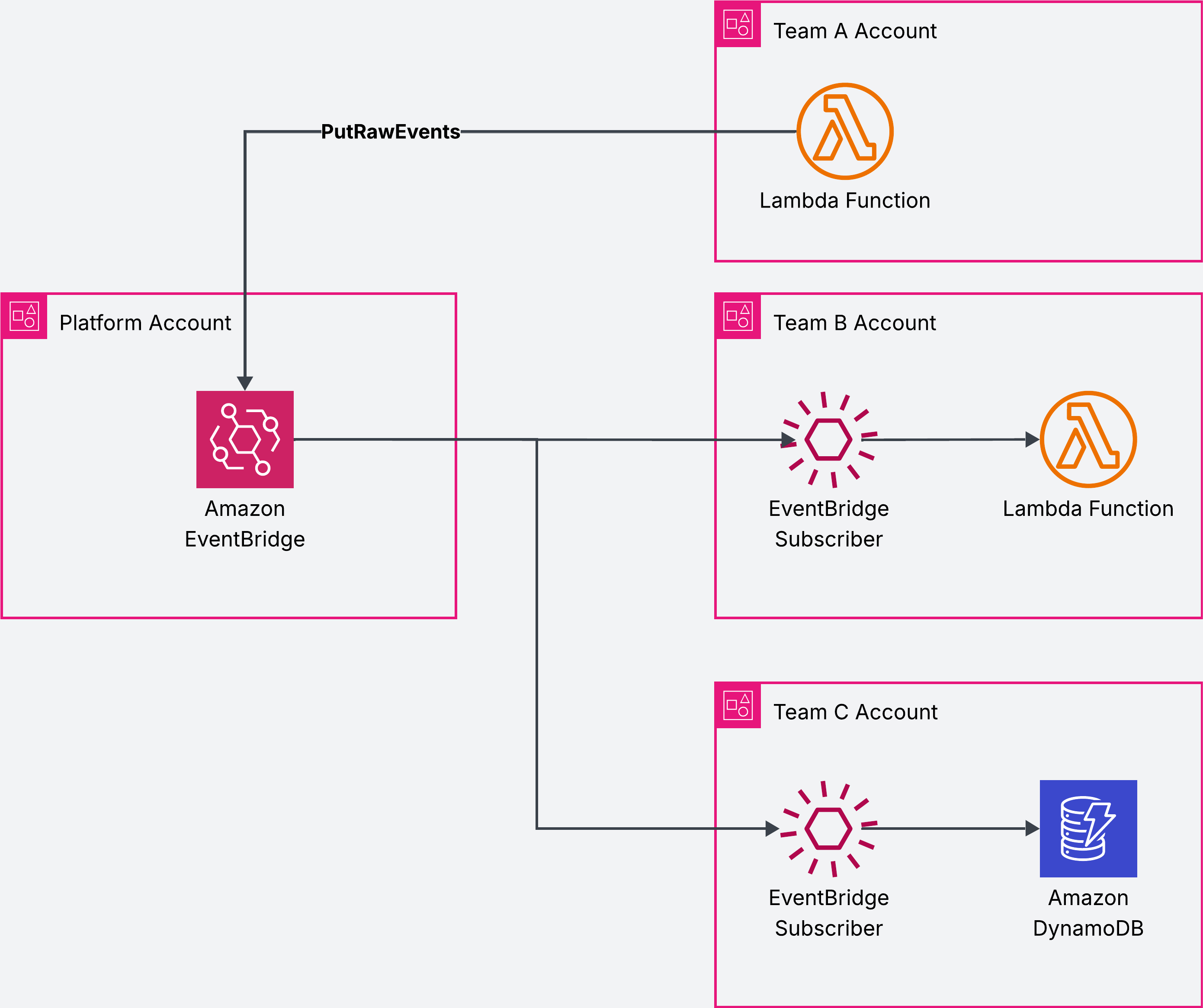
Figure 1: Multi-account sharing

Cost follows team boundaries because charges separate ingestion from delivery. The account that publishes an event pays to put it on the bus, and the account that owns a Subscriber pays for what that Subscriber consumes. Each team’s usage appears on its own bill, which is what makes a shared bus something a platform team can charge back rather than a shared cost center nobody can decompose. Removing the forwarding hops also removes the duplicated ingestion and delivery those hops created: the same event reaching the same three consumers is ingested once instead of three times.

Publishing in the format teams already use

Not every producer speaks JSON. Teams that standardize event exchange across an organization often register schemas and publish compact binary payloads, because the schema is the contract between teams that deploy on their own timetables. Accepting the formats those producers already emit is simpler than changing each one to convert to JSON first.

With the new Custom event bus, application teams can publish events in Avro, Protobuf, and CloudEvents (JSON) formats. For the binary formats, a schema registry named on the request is used to deserialize the events.

There are two publish APIs, and the payload decides which one to call. PutEvents takes structured JSON with the familiar Detail, Source, and DetailType fields. PutRawEvents takes a binary payload plus metadata you define, and is the one to use for Avro, Protobuf, CloudEvents, or bytes the bus should not interpret.

import boto3

events = boto3.client("eventbridgev2")
events.put_raw_events(
    EventBusArn=BUS_ARN,
    SchemaRegistryConfiguration={"RegistryUri": GLUE_REGISTRY_ARN},
    Entries=[
        {
            "Data": avro_encoded_order,  # bytes, straight from your existing producer
            "SystemMetadata": {"ContentType": "application/avro"},
            "Metadata": {"eventType": "OrderPlaced"},
        }
    ],
)

The schema registry can be either the AWS Glue Schema Registry or the Confluent Cloud Schema Registry.

Because the bus decodes the event before filters and transformations run, a consumer subscribing to Avro events written by another team needs no schema, no decoder, and no access to the registry. It writes the same filter it would write against JSON. Producers and consumers stay decoupled, and no deserialization code has to be repeated in each consuming team.

Publishers get one more setting on the same request: deduplication. A retry that already succeeded would otherwise leave a duplicate for every consumer to handle. It works one of two ways: the bus hashes the content of each event, or it uses a deduplication ID you supply. Content-based hashing suits producers with no natural key, since two identical events hash the same. A deduplication ID fits when you already have one, such as an order ID combined with a state transition. It keeps matching even when parts of the payload differ in ways that should not count as a new event.

Self-service onboarding for application teams

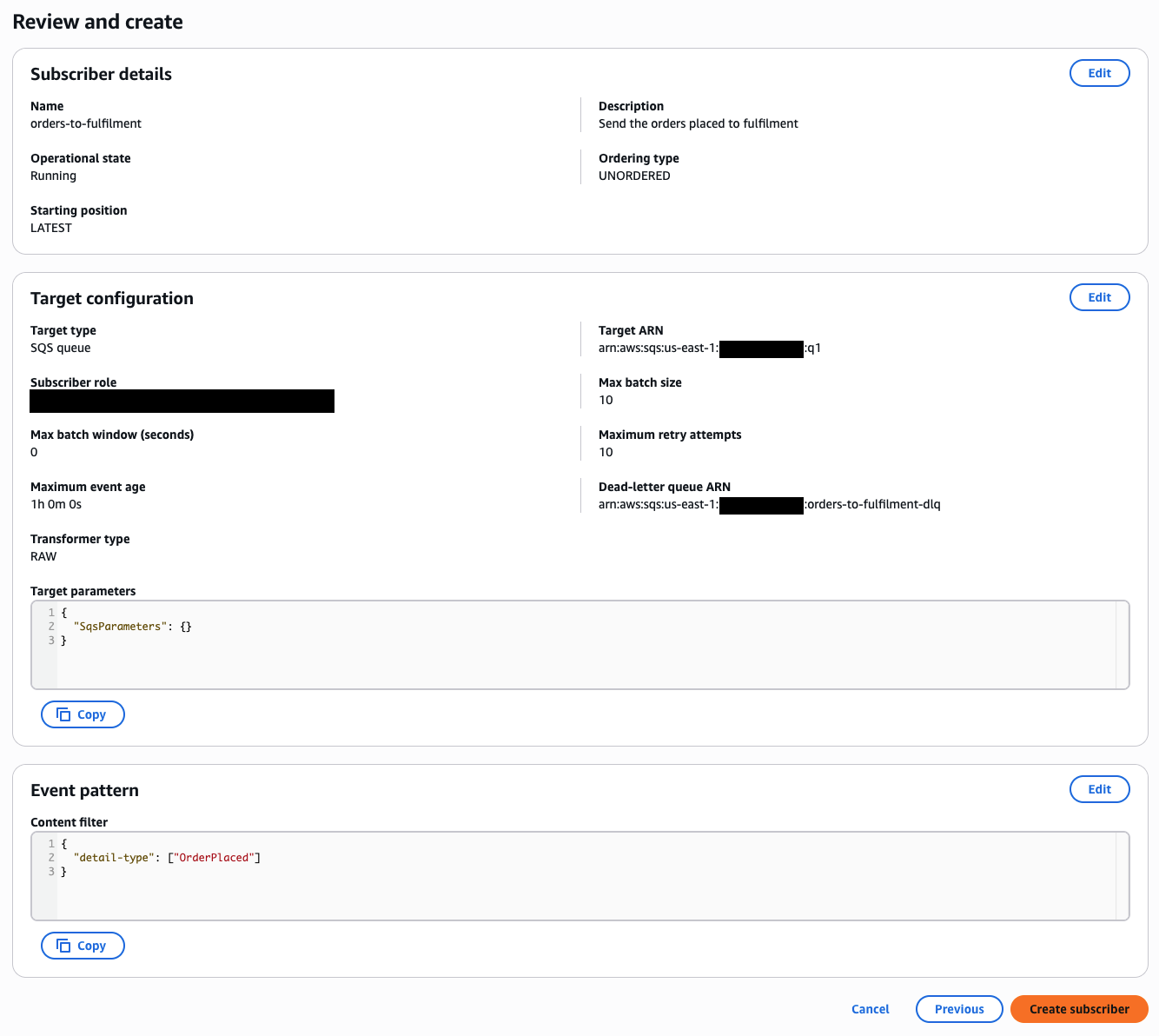
The new Custom event bus introduces a new resource called a Subscriber. Application teams create and configure their own Subscribers in their own accounts, provided they have been granted subscribe access to the bus. A Subscriber is the one place a consumer’s behavior is defined: which events it receives, where they are delivered, how delivery is retried, and where events go when delivery does not succeed. Reviewing or changing a consumer is one thing to read and one thing to update.

SUBSCRIBER_ARN=$(aws eventsv2 create-subscriber \
    --name orders-to-fulfilment \
    --event-bus-arn "$BUS_ARN" \
    --filter-configuration '{"Filters":[{"Scope":"METADATA","Pattern":"{\"eventType\":[\"OrderPlaced\"]}"}]}' \
    --invoke-configuration '{"TargetArn":"'"$QUEUE_ARN"'","RoleArn":"'"$ROLE_ARN"'"}' \
    --retry-policy '{"MaxRetryAttempts":10,"MaxEventAgeInSeconds":3600}' \
    --on-failure-configuration '{"Arn":"'"$DLQ_ARN"'"}' \
    --query SubscriberArn --output text)

A filter’s scope decides which part of the event the pattern is matched against. DATA matches the payload, METADATA matches the key-value pairs the publisher attached to the event, and SYSTEM_METADATA matches the event’s system fields: the content type and ordering key a publisher declares, plus the fields Amazon EventBridge adds itself. Because Avro and Protobuf payloads are decoded as they are published, a DATA filter reads their fields directly, the same as it would for JSON.

The retry policy says how the bus should behave when a target is failing. MaxRetryAttempts sets how many times a delivery is retried, and MaxEventAgeInSeconds sets how long an event stays eligible for retry, measured from when it was published. Retries stop as soon as either limit is reached, so both bound the same delivery.

When deliveries do fail, the reason shows up in the Subscriber’s own logs, which application teams can turn on themselves. They record the error from each delivery attempt alongside the exact input sent to the target, which makes a problem quick to place. Seeing what the target actually received separates a transformation that produced the wrong shape from a target that rejected a correct one.

Screenshot of the Amazon EventBridge console showing the Create subscriber form, with fields for the subscriber name, event bus, filter configuration, target (invoke configuration), retry policy, and on-failure destination. — Figure 2: Creating a Subscriber on console

History for consumers that did not exist yet

A Subscriber sometimes needs events that were published before it existed. For example, a new analytics service needs hydrating with recent history, or a target processed a window of events incorrectly and needs that window replayed. Because the bus retains events for the period configured on it, a Subscriber can be created with a starting position in the past, so it reads history, catches up, and continues with live traffic:

aws eventsv2 create-subscriber \
    --name analytics-backfill \
    --event-bus-arn "$BUS_ARN" \
    --starting-position POINT_IN_TIME \
    --point-in-time-configuration '{"PointType":"TIMESTAMP","StartingPoint":"2026-09-14T06:00:00Z"}' \
    --filter-configuration '{"Filters":[{"Scope":"METADATA","Pattern":"{\"eventType\":[\"OrderPlaced\"]}"}]}' \
    --invoke-configuration '{"TargetArn":"'"$ANALYTICS_ARN"'","RoleArn":"'"$ROLE_ARN"'"}'

A starting position is either LATEST or POINT_IN_TIME. Choosing POINT_IN_TIME then needs a point-in-time configuration: a PointType of TIMESTAMP with a starting point, or HORIZON to begin at the earliest event still retained. An optional end point stops the read at a chosen time, which is what you want when reprocessing a known-bad window rather than catching up to live traffic.

Two things to keep in mind. The starting position is fixed when the Subscriber is created, so reading a different window means a new Subscriber. Treat the starting position as part of a Subscriber’s identity rather than a dial to turn later. And retention cannot reach back beyond the retention window, so the read starts at the earliest retained event however far back the timestamp asks for.

Order, where order matters

In event-driven architectures, where components are built to work asynchronously, the order events arrive in usually does not matter. There are still use cases where a consumer relies on ordered delivery, and the new Custom event bus offers it as an option on individual Subscribers.

Ordering is scoped by a key the publisher sets. A publisher includes an event group ID (a customer ID, an order ID, a driver ID), and a Subscriber created with FIFO delivery type receives the events for each group in the order they were published. A FIFO Subscriber reading events published without a group ID has nothing to sequence by, so the two sides work together. Creating one takes the same call as an unordered Subscriber, with the delivery type set to FIFO:

aws eventsv2 create-subscriber \
    --name inventory-ordered \
    --event-bus-arn "$BUS_ARN" \
    --type FIFO \
    --filter-configuration '{"Filters":[{"Scope":"METADATA","Pattern":"{\"eventType\":[\"OrderPlaced\"]}"}]}' \
    --invoke-configuration '{"TargetArn":"'"$FIFO_QUEUE_ARN"'","RoleArn":"'"$ROLE_ARN"'","SqsParameters":{"MessageGroupId":"{% $events.SystemMetadata.EventGroupId %}","MessageDeduplicationId":"{% $events.SystemMetadata.DeduplicationId %}"}}'

Ordering is per group, so throughput scales with the number of groups. If an event cannot be delivered, it holds up the rest of its own group while other groups keep moving. Choosing the key therefore matters: one that maps to a business entity, such as an order or a customer, gives sequencing where it is needed and independence everywhere else. A key so broad that most events share it puts them all in a single sequence, and a key so specific that every event has its own leaves nothing to order.

Because ordering is set on each Subscriber, consumers of the same events do not need to agree on it. An inventory service can receive a group’s events in sequence while an analytics service subscribing to those same events takes them as they arrive.

Reshaping events, and delivering directly to a target

A consumer’s business logic expects events in a particular shape, and the events on the bus are not always in that shape. Where the two get reconciled is an ownership decision: inside the consumer, where it becomes part of that team’s code, or on the Subscriber, ahead of it.

The first case is reformatting. A downstream system, often owned by another domain or outside the organization entirely, expects a different structure from the one the publisher emits. A JSONata transformer on the Subscriber produces that structure before delivery, so the consumer receives what it already expects. The business logic stays where it belongs, and when the published shape changes upstream, or another event type needs deriving into the same input, it is the transformer that changes rather than the consumer:

--transformer '{
    "Type":"JSONATA",
    "JsonataConfiguration":{
        "Expression":"{% {\"orderRef\": $events.Data.detail.orderId, \"total\": $events.Data.detail.amount} %}"
    }
}'

The transformer type determines the shape of what gets delivered. RAW delivers the event payload as is and is the default, so a Subscriber with no transformer configuration receives only the payload. WITH_METADATA adds the event envelope alongside it, and JSONATA reshapes it with an expression wrapped in {% %}.

The transformation reshapes events only for the Subscriber that owns it and does not affect what other Subscribers of the same bus receive. That also makes it a data minimization control: a partner can receive only the fields it needs rather than a whole internal event. Defining it at the Subscriber means it holds for every event without anyone remembering to strip fields.

The second case is calling an AWS service API. A Subscriber delivers directly to targets including Amazon Simple Queue Service (Amazon SQS), Amazon Simple Notification Service (Amazon SNS), AWS Lambda, and Amazon Kinesis Data Streams. For other services it has been common practice to add a proxy step whose only job is to make the call. With universal targets, the new Custom event bus can call a supported AWS service API directly, with the request body built by a JSONata expression.

TargetArn: arn:aws:events:::aws-sdk:dynamodb:putItem
UniversalTargetParameters.Input:
{% { "TableName": "orders", "Item": { "pk": { "S": $events.Data.detail.orderId } } } %}

Note that a universal target shapes its input through that parameter rather than through the preceding transformer, and setting a transformer on one is rejected when the Subscriber is created. The two mechanisms do the same kind of work on different targets.

That removes the proxy processing that existed only to make the call. The delivery role still needs the action the target requires and getting that wrong is the most common cause of a Subscriber that looks healthy and delivers nothing.

Conclusion

Running an event-driven application across many accounts no longer means running many event buses and the forwarding between them. A platform team creates one new Custom event bus, shares it across the organization through AWS Resource Access Manager or a resource policy on the bus, and keeps one place to decide who publishes and who consumes. Application teams create and own their Subscribers without waiting for provisioning. Ingestion and delivery are charged separately, so each team’s usage appears on its own bill, and the duplicated ingestion that forwarding hops created disappears with the hops.

The capabilities that used to send individual teams elsewhere now sit on the same bus. Ordering is per Subscriber and scoped by a publisher-supplied key, so one team’s sequencing requirement no longer fragments an architecture. Retention makes it possible to onboard a consumer that needs history it was never subscribed to. Avro and Protobuf are decoded by the bus, so producers keep their binary contracts. Transformation and universal targets keep business logic where it belongs, removing the proxy steps that existed only to reshape an event or make an API call.

Because the new Custom event bus runs alongside the Custom event bus – classic, adoption is incremental. Point one new consumer at a shared bus or forward a slice of an existing bus into it and move the rest as teams are ready.

Next steps. Create a bus, add a Subscriber, and publish an event, starting from the Amazon EventBridge documentation for the resource model and the AWS Command Line Interface (AWS CLI) reference. If you already run Custom event buses, the migration guidance covers routing existing events into a new Custom event bus without changing producers. From there, look at the Subscriber logging and metrics options for tracing an event from publication to delivery, and at AWS Resource Access Manager for how sharing and permissions work across an organization. If you have questions or feedback about the new Custom event bus, leave a comment on this post. We’d like to hear how you’re using it.

Improving Lambda function latency with scalable network bandwidth

2026-09-29 Rahul Shandilya

Post Syndicated from Rahul Shandilya original https://aws.amazon.com/blogs/compute/improving-lambda-function-latency-with-scalable-network-bandwidth/

AWS Lambda now supports scalable network bandwidth for functions configured with 2,048 MB of memory or more, running outside of a virtual private cloud (VPC). Previously, sustained network throughput was capped at 625 Mbps regardless of your function’s memory configuration. Now, sustained throughput scales proportionally from 625 Mbps at configurations below 2,048 MB up to 3,000 Mbps at 10,240 MB, increasing the rate at which data moves to and from your execution environment.

In this post, you learn how to apply this new capability to latency-sensitive data processing workloads, helping reduce function execution times and per-invocation costs while improving the end-user experience through reduced latency. You also walk through a deployable implementation that demonstrates the performance improvements this capability unlocks.

Latency-sensitive data processing

Latency-sensitive data processing applications are data processing workloads that must be completed in a defined period of time. They often experience bursty, ad hoc traffic patterns while being required to download gigabytes or even terabytes of data from a data store, process it in a compute environment, and return a result to a waiting end user.

Latency-sensitive data processing is often highly parallelizable. Data can be divided into smaller pieces with each piece being individually processed before combining them together to obtain a result.

These workloads can be found in multiple industries and verticals. Examples include:

Log querying engines – An end user initiates an on-demand search across terabytes of log data and expects results within seconds.
Insurance underwriting – A prospective customer submits an application, triggering real-time evaluation of historical claims and risk data. The underwriting process determines what coverage and premiums to offer to the prospective customer.
Financial ETL pipelines – An economic announcement triggers an unexpected burst of market data that must be ingested, transformed, and made available to downstream trading systems before the next market tick.
Genomics platforms – A clinician orders a diagnostic test, requiring gigabytes of DNA or RNA sequencing data to pass through a bioinformatics pipeline and be compared against a reference genome while the patient awaits results.

These workloads are challenging to build on traditional compute clusters. Their spiky and unpredictable nature forces you to choose between under-provisioning compute to optimize costs (and risk missing your SLA) or over-provisioning and paying for idle capacity.

Why Lambda fits latency-sensitive data processing

Lambda eliminates this tradeoff. Instead of pre-provisioning a compute cluster, Lambda scales compute capacity in response to incoming requests, matching processing power to unpredictable traffic patterns. Because latency-sensitive data processing is highly parallelizable, the ability of Lambda to rapidly scale out execution environments makes it a natural fit. You can fan out across thousands of concurrent functions to process data in parallel, paying only for the compute you use.

However, as data volume and performance requirements grow, network bandwidth to and from the compute environment can become the limiting factor in minimizing workload latency.

Scalable network bandwidth directly addresses this limitation by raising the per-environment network throughput ceiling, improving the rate at which data can be transferred to and from the execution environment. Each execution environment can now drive up to 3,000 Mbps of sustained throughput when configured with 10,240 MB of memory, a 4.8x increase from the previous ceiling of 625 Mbps. Combined with the ability of Lambda to scale out at a rate of 1,000 execution environments every 10 seconds, you can download more than 3 TB of data in under 10 seconds.

New network throughput behavior for Lambda functions

Scalable network bandwidth applies to both data ingress to and egress from an execution environment for functions outside of a VPC. For functions configured with 2 GB of memory or more, network bandwidth scales by approximately 280 Mbps increments for every 1 GB of additional memory allocated.

The following table shows the maximum sustained bandwidth available to each execution environment at each memory configuration.

Memory Configuration	Max Sustained Bandwidth
Less than 2,048 MB	625 Mbps
2,048 MB	765 Mbps
3,072 MB	1,044 Mbps
4,096 MB	1,324 Mbps
5,120 MB	1,603 Mbps
6,144 MB	1,883 Mbps
7,168 MB	2,162 Mbps
8,192 MB	2,441 Mbps
9,216 MB	2,721 Mbps
10,240 MB	3,000 Mbps (4.8x increase)

Table 1. Lambda sustained network bandwidth by memory configuration. Bandwidth scales at ~280 Mbps per additional GB of memory above 2 GB.

In the following section, you learn how scalable network bandwidth improves end-user latency by building an ETL pipeline that demonstrates it. You can find the source code in the GitHub repository.

Solution overview

Consider a SaaS analytics platform where users submit ad hoc queries against a data store. The application must extract the relevant data, apply a filter or transformation, and return an aggregate result while the user waits. In this example, the result needs to be returned in 8 seconds or less.

The following diagram illustrates the architecture of the solution.

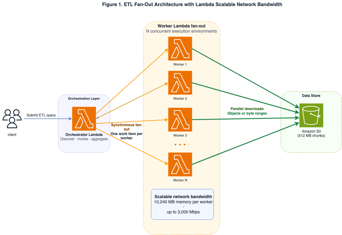
ETL fan-out architecture: a client calls an orchestrator Lambda function, which fans out to multiple worker Lambda functions that read data in parallel from Amazon S3, with bandwidth scaling callouts for each memory tier.

Figure 1. ETL fan-out pattern: an orchestrator Lambda function distributes work to multiple worker Lambda functions that read from Amazon S3 in parallel, with bandwidth scaling callouts per memory tier.

A client initiates an ad hoc query by calling the orchestrator Lambda function through the Lambda API. The orchestrator function determines how to split the work. To process the data in parallel, the orchestrator function uses a ThreadPoolExecutor to issue synchronous invoke requests to the Lambda worker function, fanning out the worker across multiple execution environments at the same time.

Each Lambda worker function is configured with 10,240 MB of memory, so it has access to up to 3,000 Mbps of sustained network throughput. After the data is processed, the aggregated result is returned to the client.

Prerequisites

Before you start the deployment process, make sure that you have completed the following steps:

Install the AWS SAM CLI on your computer and confirm that you are running Python 3.12 or later.
Have your AWS account credentials ready.
Submit a request to AWS Service Quotas to turn on scalable network bandwidth for your Lambda functions. This quota is listed under Network bandwidth per execution environment.

Clone the source code from the GitHub repo and deploy the application within your AWS account. Creating the 10 GB test dataset and running the benchmark can incur charges to your AWS account.

git clone https://github.com/aws-samples/sample-lambda-enhanced-bandwidth
cd sample-lambda-enhanced-bandwidth
sam build
sam deploy --guided

After the AWS CloudFormation stack is deployed, record the DataBucketName and orchestrator function name from the stack outputs to use in subsequent commands.

To simulate data for the end user to query, the GitHub repo has a script that creates 10 GB of synthetic data and uploads it to your S3 bucket.

Mode 1: Processing pre-partitioned data

In Mode 1, the 10 GB of synthetic data is pre-partitioned. Pre-partitioned data is typically produced incrementally by many sources over a period of time, which can be the case with IoT data or access logs. The following command creates 10 GB of data divided into 20 partitions that are 512 MB each.

python scripts/generate_data.py \
    --bucket <DATA_BUCKET_NAME> \
    --total-gb 10 \
    --chunk-mb 512

Turning on scalable network bandwidth does not, on its own, make your downloads faster. A single download request only opens one connection to Amazon S3, and one connection does not move data fast enough to fill all the bandwidth now available to your Lambda function. To actually use your full allotment of network bandwidth, the execution environment has to pull the data over several connections at once. It does this by preferring the AWS Common Runtime (CRT) transfer client, a high-performance download engine built into Boto3. When the worker calls download_fileobj, the CRT client automatically breaks the 512 MB object into smaller parts and downloads them in parallel across multiple Amazon S3 requests. Those parallel downloads are what let a single Lambda worker take advantage of its full network bandwidth.

The following command runs the benchmark on the pre-partitioned data.

python scripts/run_fanout_benchmark.py \
    --orchestrator-name <STACK_NAME>-orchestrator \
    --bucket <DATA_BUCKET_NAME> \
    --iterations 5

Mode 2: Processing single large objects

Mode 2 generates 10 GB of data in one large object. This arrangement is more common when data is produced or delivered as one complete unit, such as database backups or genomic datasets. The following command creates 10 GB of data in a single large object.

python scripts/generate_data.py \
    --bucket <DATA_BUCKET_NAME> \
    --single-object-gb 10 \
    --key large-object/large-file.bin

In Mode 1, the CRT preference applies to Boto3 managed transfer methods such as download_file and download_fileobj. Mode 2 takes a different approach. Each worker reads a specific byte range of a single large object using get_object. The CRT preference setting has no effect on these calls. Instead, you can control concurrency by explicitly tuning the number of Lambda workers and using a bounded ThreadPoolExecutor to issue multiple byte-range requests at the same time.

When you run the following command, the orchestrator takes the single large object and divides it into consecutive byte ranges of 512 MB each. Each of the individual ranges is then processed by a Lambda worker execution environment in parallel.

python scripts/run_fanout_benchmark.py \
    --orchestrator-name <STACK_NAME>-orchestrator \
    --bucket <DATA_BUCKET_NAME> \
    --key large-object/large-file.bin \
    --slice-size-mb 512 \
    --iterations 5

The benchmark reports wall-clock duration, client-observed duration, aggregate throughput across workers, worker completion counts, and target compliance. When comparing memory configurations, keep the code, dataset, AWS Region, partition count, warm-up policy, and measurement count identical. You should run the benchmark multiple times in your account because placement, cold starts, concurrency, S3 behavior, and execution-environment reuse could affect results.

Results

To compare results, we ran the benchmark using a baseline configuration where the worker Lambda function is configured with only 1,024 MB of memory, well below the 2,048 MB threshold required for scalable network bandwidth to take effect. The 1,024 MB configuration limits network throughput to the previous sustained ceiling of 625 Mbps.

In our baseline test run, a worker downloaded and processed a single 512 MB partition with a 6.61-second download time at a 649.8 Mbps throughput (at p50). The 649.8 Mbps throughput exceeds the 625 Mbps ceiling because Lambda is capable of bursts in network throughput over a short period of time. Across twenty measured fan-out queries, the complete 10 GB query was completed with a 7.113-second wall-clock at p50. This fits within the 8-second SLA but leaves very little headroom.

To run our scalable network bandwidth benchmark, we re-deployed our worker Lambda function with a 10,240 MB memory configuration and re-ran the application. At a 10,240 MB memory configuration, each execution environment can now access up to 3,000 Mbps in sustained throughput. Direct 512 MB downloads achieved a 1.70-second download time and 2,521.3 Mbps throughput (both at p50). The complete 10 GB query was completed with a 2.640-second wall-clock at p50. That is 2.69 times faster, or 62.9% lower median latency, than the 1,024 MB configuration.

Table 2 summarizes the direct worker and end-to-end fan-out measurements for the same 10 GB dataset and 20 × 512 MB orchestration pattern. Aggregate throughput is the total data transfer rate across all twenty execution environments spun up to run the benchmark.

Memory Configuration	Single 512 MB partition download time and throughput (p50)	10 GB fan-out wall time (p50)	Aggregate throughput p50
1,024 MB baseline tier (sustained 625 Mbps)	6.61s / 649.8 Mbps	7.113s	12.08 Gbps
10,240 MB scalable tier (up to 3,000 Mbps)	1.70s / 2,521.3 Mbps	2.640s	32.54 Gbps

Table 2. Measured 1,024 MB baseline tier and 10,240 MB scalable bandwidth performance for a 10 GB fan-out ETL query.

Using scalable network bandwidth, the customer’s SLA headroom has improved by nearly 5 seconds. The Lambda function can now handle larger partitions within the same SLA window, reducing costs while still remaining comfortably within the customer’s SLA.

Clean up

To clean up the resources you created for the benchmark test, run the following commands:

aws s3 rm s3://<DATA_BUCKET_NAME> --recursive
sam delete --stack-name <STACK_NAME>

Best practices

After scalable network bandwidth is turned on for your AWS account, the following practices help you get the most out of it.

Profiling and planning

Test before you tune. Not every function is network-bound. Before increasing memory, profile your function to confirm that network I/O is the primary contributor to invocation duration and not CPU or application logic. Use Amazon CloudWatch Lambda Insights to inspect rx_bytes, tx_bytes, and duration. Functions where network I/O dominates invocation time are prime candidates for tuning.
Design for parallelism. Break your data into parallelizable chunks that can be processed independently in a fan-out pattern across multiple execution environments. You can use Amazon S3 byte-range reads to split large files into independently downloadable partitions. For implementation details, see Downloading an object with part numbers in the Amazon S3 User Guide.
Run AWS Lambda Power Tuning. Lambda Power Tuning is a state machine that helps you optimize your Lambda functions for cost and performance. Use Power Tuning to sweep memory configurations from 1,024 MB to 10,240 MB and identify the optimal cost-vs-latency point for your workload.

Implementation

Check upstream and downstream limits. Check the throughput limits of your data sources. For example, a Lambda function running at 3,000 Mbps can exceed the throughput capacity of a single S3 prefix, which supports up to 5,500 GET requests per second. When this happens, you will see HTTP 503 (Slow Down) errors in your application logs. Distribute your S3 objects across multiple prefixes to parallelize reads and avoid per-prefix throttling.
Balance bandwidth and CPU. Lambda allocates CPU proportionally to memory. For example, at a 1.7 GB memory configuration you are allocated 1 vCPU while a 10 GB memory configuration is allocated up to 6 vCPU. If your function processes data in parallel threads, the higher memory tiers give you both more network bandwidth and more CPU to process it. Use the concurrent.futures module in Python or worker_threads in Node.js to process data across parallel threads and maximize both CPU and network utilization.
Turn on Amazon S3 CRT for Boto3. If your function uses the Python runtime, initialize your Amazon S3 client with preferred_transfer_client: 'crt' to maximize single-connection throughput. The AWS Common Runtime automatically parallelizes requests across multiple TCP connections, which matters because individual TCP connections have a throughput ceiling.
Use SnapStart for JVM workloads. If you use Lambda SnapStart for Java functions, scalable network bandwidth reduces afterRestore hook latency. Network activity that occurs during function restore, such as pre-warming connections or pre-fetching configuration data, can complete faster.

Conclusion

Scalable network bandwidth raises the per-environment sustained throughput ceiling of AWS Lambda from 625 Mbps to 3,000 Mbps, directly reducing end-to-end latency for data-intensive workloads. Combined with the Lambda scaling rate, you can now move terabytes of data in seconds, without provisioning or managing infrastructure.

To get started, request the Network bandwidth per execution environment quota increase through AWS Service Quotas and deploy the sample application from the GitHub repository to see the improvement firsthand.

Republicans Jailbreak From Trump

2026-09-28 The Atlantic

Post Syndicated from The Atlantic original https://www.youtube.com/watch?v=GfXIxpD_1vY

How Property Finder automated incident management with AWS DevOps Agent

2026-09-28 Nada Tlohi

Post Syndicated from Nada Tlohi original https://aws.amazon.com/blogs/devops/how-property-finder-automated-incident-management-with-aws-devops-agent/

When a production service starts saturating the CPU at 1 AM, every minute counts for incident management. For Property Finder, a production incident could mean failed searches, frustrated users, and direct revenue impact. Property Finder is the leading property portal in the Middle East and North Africa (MENA), serving millions of property seekers across five markets.

Before adopting AWS DevOps Agent, incident response followed a familiar pattern: an alert fires, an on-call engineer wakes up, spends 20–40 minutes correlating metrics across tools, manually documents findings, and opens a fix. Mean Time to Resolution stretched to 2–3 days for non-critical issues.

Today, that entire workflow runs autonomously. From alert to root cause analysis, Slack notification, Jira ticket, on-call phone call with context, and auto-remediation pull request (PR), the full lifecycle completes in 14 minutes. This post walks through the implementation and shows how a separate custom agent that automatically generates code fixes is the key differentiator.

The business problem

Property Finder runs a distributed microservices architecture on Amazon Elastic Container Service (Amazon ECS) fronted by Application Load Balancers (ALBs). When infrastructure issues occur, the impact is immediate: users see failed searches, agents cannot update listings, and revenue is directly impacted during peak hours.

The traditional workflow had three gaps:

Detection lag. Non-critical anomalies could go undetected for days.
Context switching. Engineers bounced between five or more tools per incident.
Knowledge silos. Runbooks lived in people’s heads, not automation.

Solution architecture

Property Finder’s implementation connects AWS DevOps Agent at the center of a three-tier pipeline: Detection and Trigger, Autonomous Investigation, and Event-Driven Output.

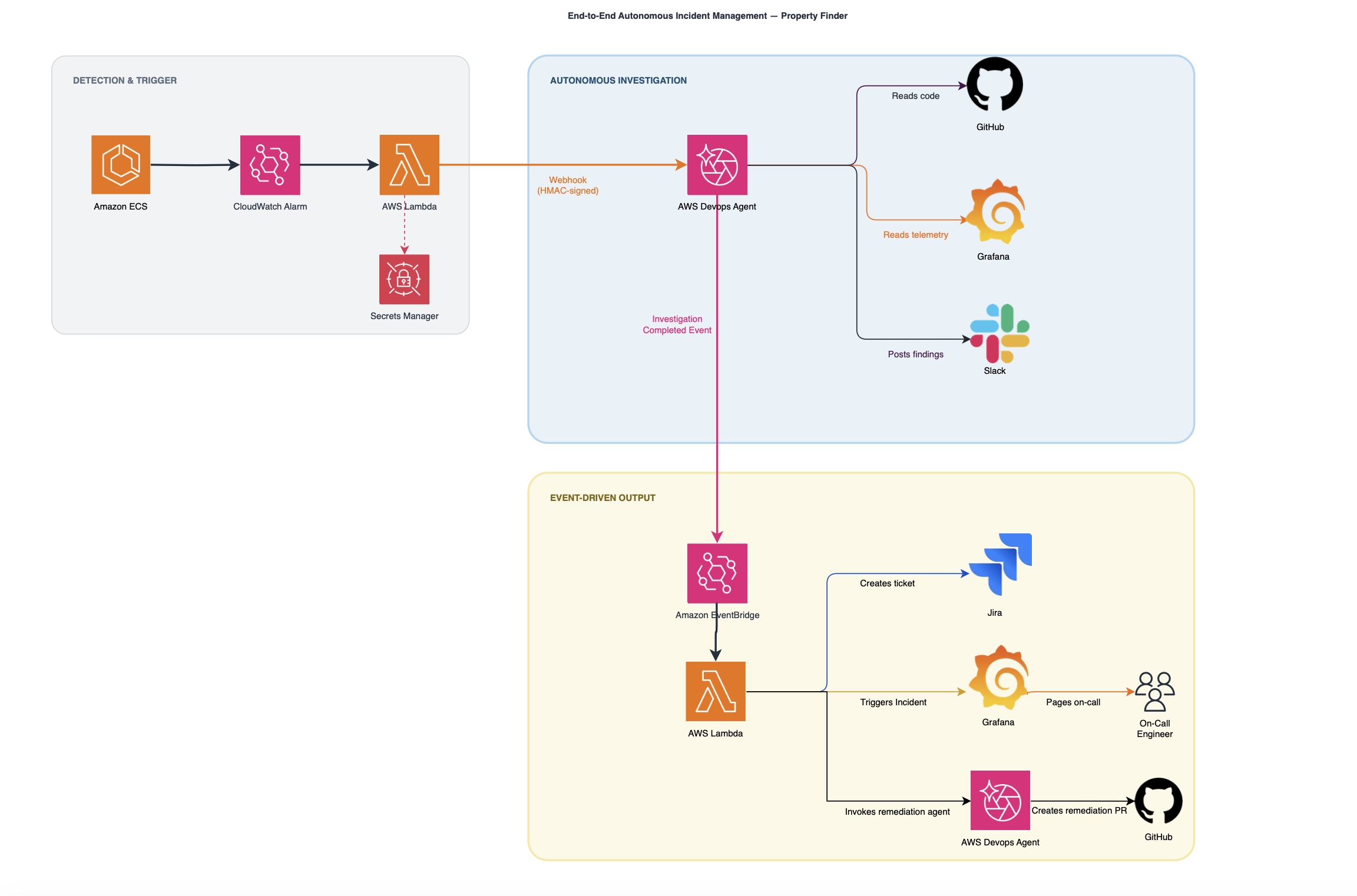
Three-tier incident pipeline from a CloudWatch alarm through AWS DevOps Agent investigation to Slack, Jira, and GitHub outputs

Figure 1: End-to-end autonomous incident management architecture

The numbered steps correspond to the data flow in Figure 1:

ECS CPU spike triggers an Amazon CloudWatch Alarm. CloudWatch Metrics Insights monitors service health across all ECS clusters. When sustained CPU exceeds 98%, the alarm transitions to ALARM state.
AWS Lambda formats and HMAC-signs the payload. Triggered directly by the CloudWatch alarm action (which fires only on ALARM state transitions), AWS Lambda enriches the payload with service metadata, signs it with HMAC-SHA256 using credentials from AWS Secrets Manager, and POSTs to the webhook.
The agent begins autonomous investigation. Parallel subagents query ECS metrics, AWS CloudTrail, ALB traffic patterns, and Grafana telemetry (Prometheus, Loki, Pyroscope). The agent reads relevant source code from GitHub for correlation.
Findings post to Slack in real time. The native Slack integration posts investigation progress to #incidents. The full root cause analysis, impact assessment, and mitigation plan appear at the end of the thread.
Investigation Completed event fires to Amazon EventBridge. Amazon EventBridge triggers an orchestrator Lambda that fans out to three independent targets simultaneously.
Lambda creates a Jira ticket with the full root cause analysis. The Lambda retrieves the investigation summary from journal records and creates a prioritized ticket with root cause, severity, and affected service.
Grafana IRM pages the on-call engineer by phone. A Lambda posts a Grafana Alerting-compatible payload to the IRM webhook. The escalation chain calls the engineer with full investigation context: what broke, why, and the recommended fix.
The remediation agent opens a GitHub PR with the auto-fix. It receives the root cause, generates a Terraform or code fix, and opens a Draft PR through a GitHub Model Context Protocol (MCP) server. Engineers review before merging.

A real incident

The example-service, Property Finder’s core property search microservice serving millions of queries per day across five MENA markets, experienced CPU saturation at 99.11%. The pipeline resolved it end-to-end in 14 minutes.

1:21 AM │ Alarm fires (ECS CPU > 98%)

1:22 AM │ Investigation starts + Slack posted

1:22 AM │ 4 parallel subagents launched

1:32 AM │ Root cause identified

1:33 AM │ Jira ticket [redacted] created

1:34 AM │ On-call paged via phone call

1:35 AM │ GitHub PR [redacted] opened with fix

The detection Lambda handles three tasks: (1) retrieves the webhook secret from AWS Secrets Manager, (2) enriches the CloudWatch alarm event with ECS service metadata (cluster name, service name, task count), and (3) HMAC-signs the payload before POSTing to the webhook. The key authentication pattern:

# HMAC-SHA256 signing for webhook authentication
ts = datetime.now(timezone.utc).strftime("%Y-%m-%dT%H:%M:%S.000Z")
body = json.dumps(incident)
sig = hmac.new(webhook_secret.encode("utf-8"),
               f"{ts}:{body}".encode(), hashlib.sha256).digest()
http.request("POST", webhook_url, body=body,
             headers={"x-amzn-event-timestamp": ts,
                      "x-amzn-event-signature": base64.b64encode(sig).decode()})

Four parallel subagents querying ECS, CloudTrail, ALB, and Grafana data sources during the investigation

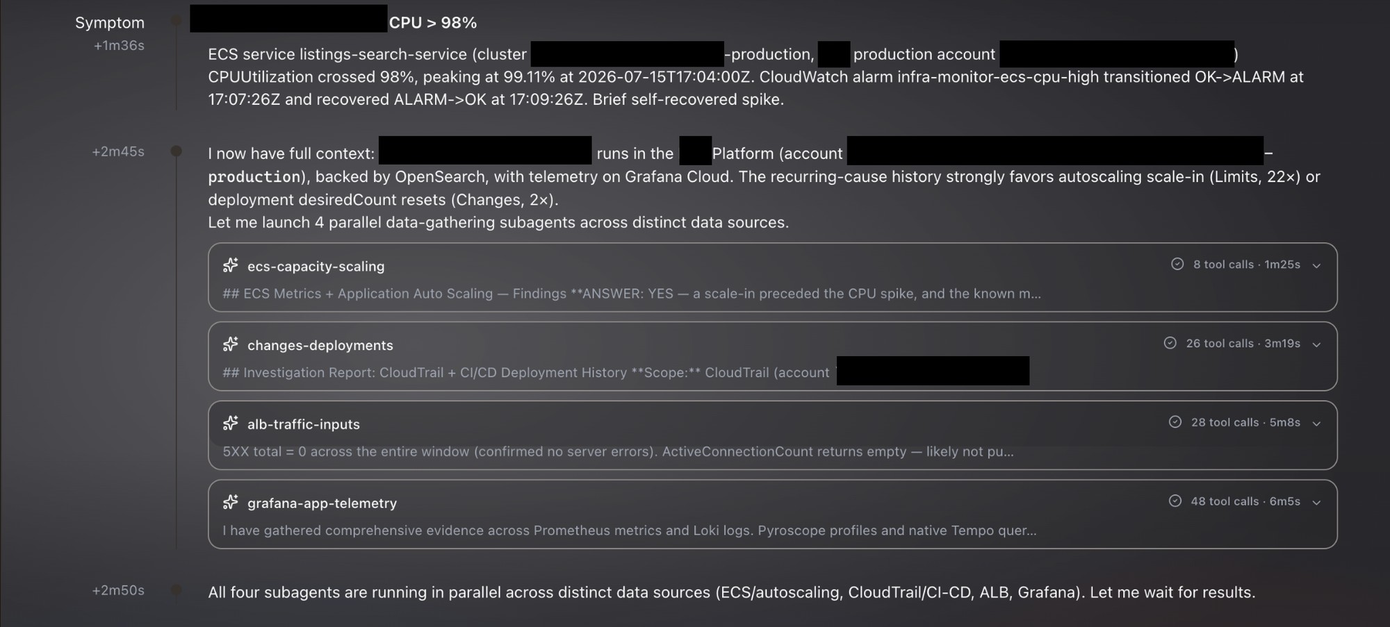
Figure 2: Four parallel subagents investigating ECS, CloudTrail, ALB, and Grafana data sources simultaneously

Root cause: Conflicting CPU and memory target-tracking autoscaling policies combined with an insufficient capacity floor. The service had both a CPU policy (target 70%) and a memory policy (target 75%). Actual memory usage sat at 3–8%, creating a persistent conflict between the two policies.

With MinCapacity set too low, the service could not sustain the task count needed to absorb CPU load. The resulting instability (22+ scaling flips observed) prevented stable scale-out, leaving the service effectively pinned at two tasks with no CPU headroom.

This is a common organizational issue: teams configure both scaling dimensions without realizing the interaction, especially when the capacity floor is not sized for baseline traffic. The agent identified the pattern in 10 minutes, a task that typically requires senior engineers with deep scaling expertise and hours of CloudWatch metric correlation.

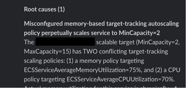
Investigation output naming conflicting CPU and memory autoscaling policies as the root cause

Figure 3: Root cause analysis identifying the conflicting autoscaling policy

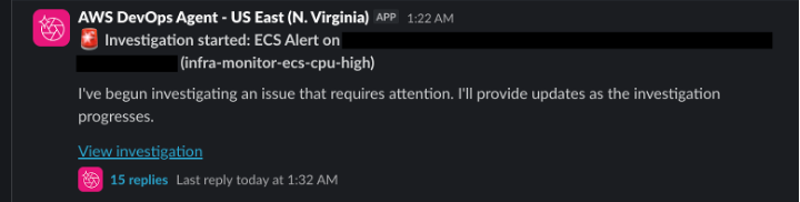
Slack incidents channel message linking to the running investigation at 1:22 AM

Figure 4: Slack notification with investigation link posted at 1:22 AM

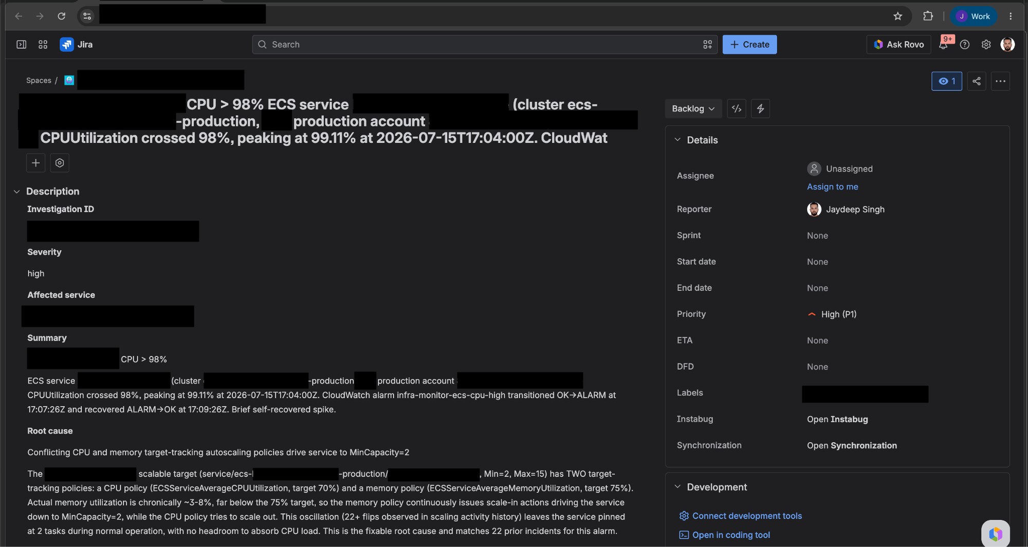
Auto-created Jira ticket showing priority, root cause, and affected service

Figure 5: Jira ticket [redacted] auto-created with priority, root cause, and affected service

At 1:34 AM, the on-call engineer received a phone call through Grafana IRM with the complete investigation context. No need to wake up and hunt for root cause across dashboards.

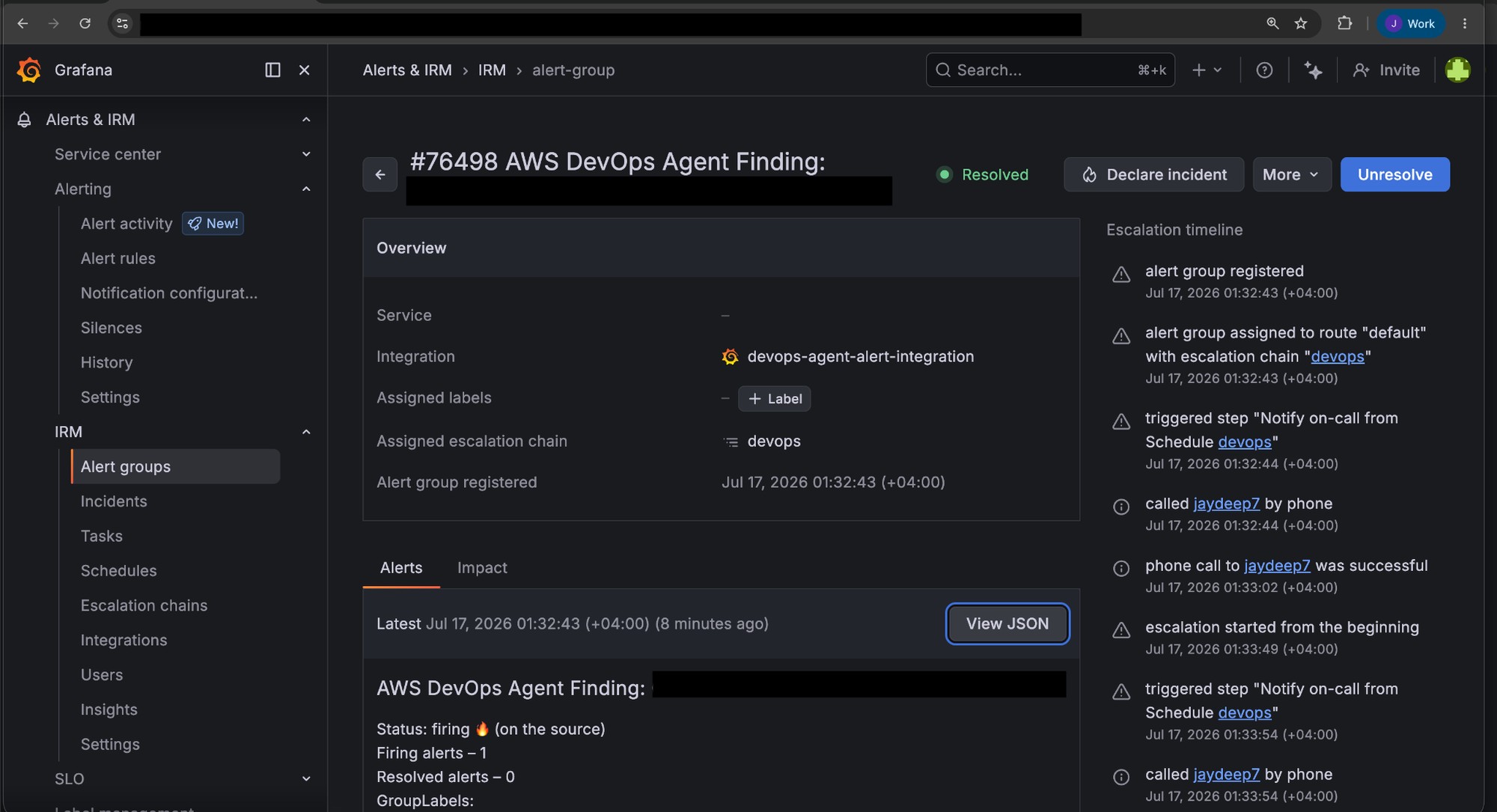
Grafana IRM escalation chain routing the alert to the on-call engineer

Figure 6: Grafana IRM escalation chain routing the alert and calling the on-call engineer

Incoming on-call phone call at 1:34 AM carrying the investigation context

Figure 7: Incoming phone call at 1:34 AM with investigation context

Mitigation plan generated: (1) Remove the memory-based scaling policy, (2) raise MinCapacity to handle baseline traffic, (3) implement CPU-only target tracking at 70%. This plan was passed to a separate custom agent for remediation.

Remediation

Remediation is the key differentiator in this pipeline. It is a dedicated remediation agent (pr-creation-agent) invoked only after investigation completes. AWS DevOps Agent enforces read-only access to infrastructure through a per-session permission guardrail. Effective permissions are the intersection of the execution role’s IAM policy and the guardrail, and write actions are excluded.

The split separates concerns: investigation stays within that read-only envelope, whereas the remediation agent is scoped to a GitHub MCP server as its only external integration. Safety at the remediation layer does not rely on the agent’s built-in directed actions approval mechanism. Instead, two controls enforce the boundary. First, the remediation agent is a separate, narrowly scoped agent with access limited to GitHub MCP. Second, every output is a Draft pull request that requires human review and merge before taking effect. The GitHub MCP connection is authenticated with a fine-grained personal access token scoped to the specific infrastructure repositories, with an expiration and rotation policy. No elevated IAM role or additional agent permissions are required.

How it works

When the “Investigation Completed” Amazon EventBridge event fires, a Lambda orchestrator invokes the remediation agent with the investigation ID. The agent then:

Reads findings from journal records to understand the root cause and recommended fix.
Maps the AWS account to the correct repository. Property Finder has six infrastructure repos for different teams (B2B, B2C, core-platform, growth, data-engineering, shared-infra). The agent extracts the account ID from resource ARNs and routes to the right repo. This mapping is validated through automated tests and updated as new accounts or repositories are onboarded.
Checks for duplicate PRs by searching existing PR titles and bodies for the investigation ID. If a matching PR exists, it reports the URL and exits without creating a duplicate.
Reads the relevant Terraform files through GitHub MCP (GITHUB-MCP_get_file_contents), identifies the exact changes required, and plans the fix.
Creates a feature branch (fix/{investigation_id}), commits the changes, and opens a Draft PR with a structured template including problem summary, root cause, changes made, and a testing checklist.

AWS also supports remediation through Kiro CLI with AWS CodeBuild or Kiro-ready prompts. Property Finder chose an approach that fits their multi-team repository structure: the remediation agent runs entirely within the Agent Space (the managed environment where custom agents execute), uses GitHub MCP for repository access, and maps multiple repositories to different teams automatically.

The orchestrator Lambda is triggered by the “Investigation Completed” Amazon EventBridge event. It first retrieves the investigation findings from journal records, then fans out to three targets simultaneously. Target one creates a Jira ticket with the full root cause analysis, severity, and affected service. Target two posts a Grafana Alerting-compatible payload to the Grafana IRM webhook to trigger phone call escalation. Target three invokes the remediation agent through the CreateChat and SendMessage API, passing the investigation ID and root cause context so it can generate the appropriate code fix.

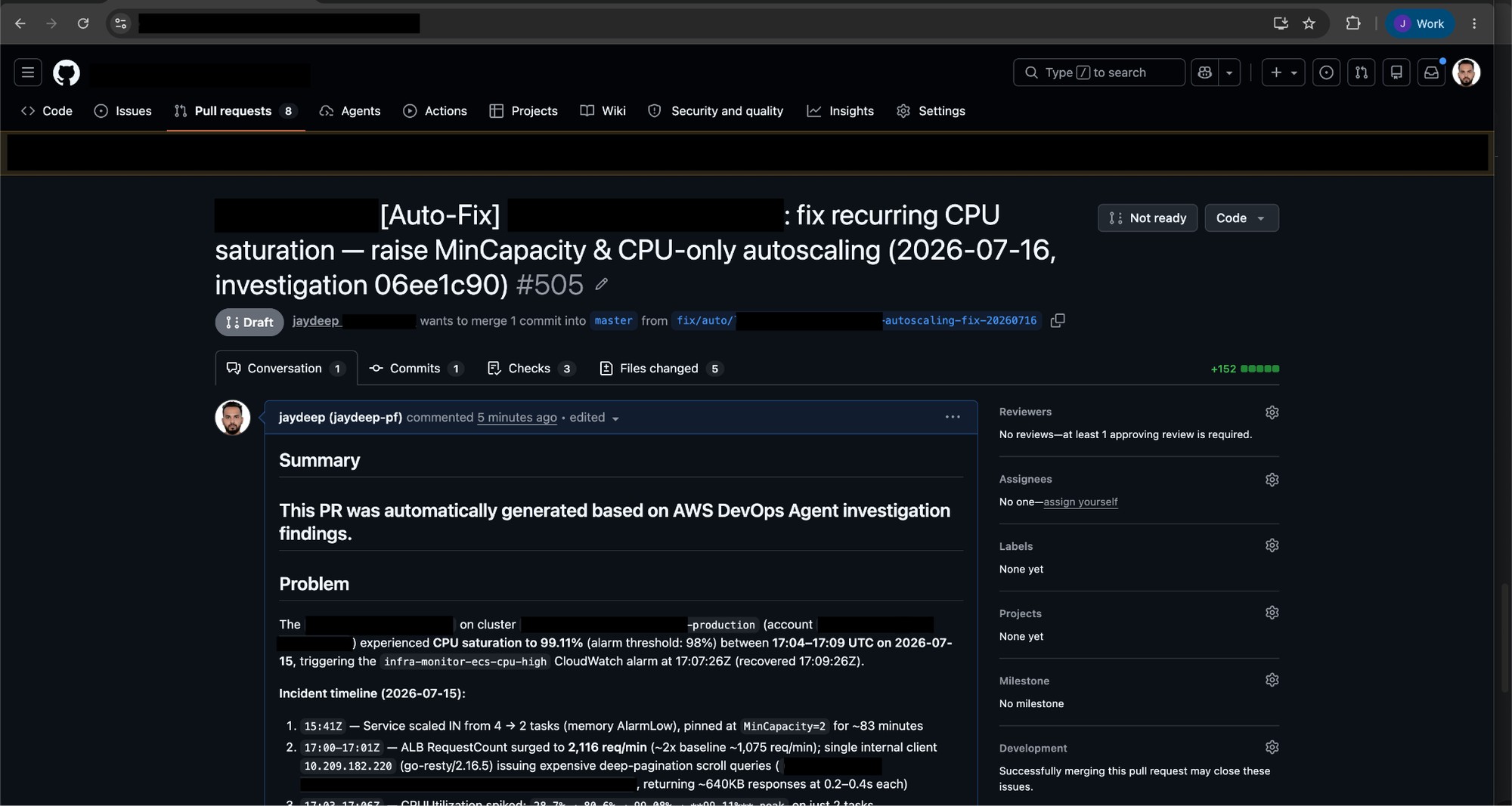
Draft GitHub pull request with a problem summary, root cause, and changes template

Figure 8: GitHub PR [redacted] generated by the remediation agent with a structured problem, root cause, and changes template

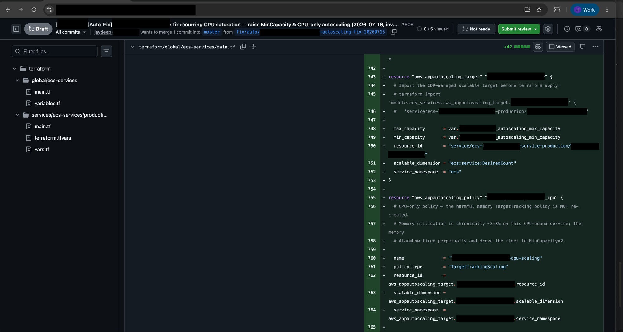
Terraform diff replacing the memory scaling policy with a CPU-only target-tracking policy

Figure 9: Terraform diff showing the new CPU-only scaling policy replacing the conflicting memory configuration

The PR is always opened as Draft. Engineers review, run terraform plan, validate in staging, and merge. The agent never auto-merges.

Results

Metric	Before	After	Improvement
End-to-end time	Hours to days	14 minutes	>88% reduction
Investigation	20 to 40 min (manual)	10 min (autonomous)	50–75% reduction
Documentation	Manual, incomplete	Auto-generated root cause analysis + Jira	100% documented
Remediation	Manual PR by engineer	Auto-fix PR + review	Minutes to code fix

Cost considerations: Each incident invokes two agent sessions (investigation + remediation) with up to four parallel subagents. Billing is based on agent minutes. For detailed pricing, see the AWS DevOps Agent pricing page. We recommend reviewing pricing for all services used in this architecture.

“We now rely fully on AWS DevOps Agent to identify infrastructure-related issues. It has helped us identify multiple complex issues without even opening a support ticket. Even if we had raised tickets, it would likely have taken support engineers hours to find the root cause, whereas we resolved these issues in minutes.”

— Yasitha Bogamuwa, Cloud Engineering Manager, Property Finder

Getting started

Prerequisites:

An Agent Space configured in your account.
Amazon CloudWatch and AWS CloudTrail enabled for observability.
Slack, Grafana, and GitHub connected as capabilities.
Infrastructure resources tagged for topology mapping.

Step 1: Configure the webhook trigger. Set up CloudWatch Alarm action to invoke a Lambda function. The Lambda enriches the payload, HMAC-signs it, and POSTs to your Agent Space webhook endpoint.

Step 2: Set up event-driven outputs. Create an Amazon EventBridge rule for “Investigation Completed” events (source: aws.aidevops). Add Lambda targets for Jira, Grafana IRM, and optionally a remediation custom agent.

Step 3: Test end-to-end. Trigger a test alarm and verify the full pipeline: investigation starts, Slack posts, Jira ticket created, on-call paged, and PR opened.

For a similar integration pattern with Salesforce, see Automating Incident Investigation with AWS DevOps Agent and Salesforce MCP Server on the AWS DevOps Blog.

Clean up

This post describes an architecture pattern implemented by Property Finder. If you deployed test resources while following along, remember to delete any CloudWatch Alarms, Lambda functions, Amazon EventBridge rules, and Agent Space configurations to avoid ongoing charges. For a full list of resources and associated costs, review the pricing pages for each AWS service used in this architecture.

Conclusion

Property Finder’s implementation shows that autonomous incident management works in production today, with their pipeline running since early 2026. The agent never auto-merges. Human review remains in the loop by design: the agent accelerates, the engineer decides. The on-call engineer wakes up to a phone call with the root cause already identified, a Jira ticket filed, and a PR ready for review.

Explore the AWS DevOps Agent documentation to get started with your own autonomous pipeline.

About the authors

Git v2.56.0 released

2026-09-28 jake

Post Syndicated from jake original https://lwn.net/Articles/1097213/

Version 2.56 of the Git distributed
version-control system has been released. It has 748 non-merge commits
since Git 2.55 was released back in
June; those commits came from 104 developers, 39 of whom are first-time
contributors. New features include a safer workflow for conflict
resolution, smaller path-walk repacks, a new git history drop
sub-command, and much more. LWN looked at Git
2.56 recently and the GitHub blog has a lengthy
look at 2.56 as well.

AWS European Sovereign Cloud: Demonstrating an independent operation

2026-09-28 Stéphane Israël

Post Syndicated from Stéphane Israël original https://aws.amazon.com/blogs/security/aws-european-sovereign-cloud-demonstrating-an-independent-operation/

On Saturday, October 24, 2026 we will conduct an exercise, demonstrating that the AWS European Sovereign Cloud can operate without depending on any infrastructure outside of the European Union (EU).

For several hours, the AWS European Sovereign Cloud will operate without a connection to the AWS Global Network backbone. The backbone is the private network that moves authorized AWS operational data between AWS locations without using the public internet. During the exercise, this traffic will securely reroute over the public internet.

The exercise will not affect service availability within the AWS European Sovereign Cloud, other AWS Regions, or private connectivity through AWS Direct Connect. Customers may experience brief connectivity disruptions as traffic moves onto a separate network route at the beginning or the end of the exercise, after which normal connectivity resumes.

The operational team, composed entirely of EU residents within the EU, will execute the exercise using only the hardware and software resources of the AWS European Sovereign Cloud. The AWS European Sovereign Cloud Managing Directors called for this exercise to showcase its operational independence.

An independent cloud for Europe

The AWS European Sovereign Cloud is a new, independent cloud for Europe. Located in Brandenburg, Germany, its data centers are physically and logically separate from other AWS Regions, with a local in-EU copy of the source code. All customer content and customer-created metadata stay in the EU. It has no critical dependencies on non-EU infrastructure and is operated exclusively by EU residents.

In standard operations, the AWS European Sovereign Cloud uses two global systems. The first is the AWS Global Network backbone. The second is a dedicated system that the local EU team controls and supervises to securely manage limited, controlled transfers of operational AWS data.

Neither is operation-critical, and neither affects the sovereignty assurance of the AWS European Sovereign Cloud. The AWS European Sovereign Cloud can operate independently at any time without a connection to these global systems, and on October 24 that’s what the team will demonstrate.

Built to meet regulatory standards

This exercise will produce verifiable technical and operational evidence that the AWS European Sovereign Cloud can operate independently within the EU. The exercise is designed to be consistent with the objectives of the European Commission’s EU Cloud Sovereignty Framework (CSF) and the criteria of the C3A framework from Germany’s Federal Office for Information Security (BSI). These frameworks set out objectives and criteria for assessing whether cloud services can be provided independently and autonomously.

We designed the AWS European Sovereign Cloud for regulated customers and the public sector across the EU. The AWS European Sovereign Cloud: Sovereign Reference Framework (ESC-SRF) gives our customers and partners a comprehensive set of evidence points, maps to controls, artifacts, and other elements regulators and compliance authorities need to accelerate their adoption of the AWS European Sovereign Cloud. The results of this exercise will provide additional evidence for their compliance and assurance packages.

Standalone and fully secure

The AWS European Sovereign Cloud runs connected to the AWS Global Network backbone because it delivers superior performance, capacity, reliability, security, and cost savings to customers. That includes always-on encryption and distributed denial of service (DDoS) defenses; and the backbone can’t decrypt or see the encrypted data that AWS European Sovereign Cloud customers send and receive. While the backbone delivers these benefits day-to-day, the AWS European Sovereign Cloud can continue to operate independently, with the appropriate security controls in place.

During the exercise, instead of using the AWS Global Network backbone, the AWS European Sovereign Cloud will exclusively use its dedicated internet connectivity from European internet service providers. This will provide connectivity to the worldwide internet.

Whenever traffic moves between internet links, there’s a small window of limited disruption called convergence, a short time when other non-AWS networks change their routing information to reflect the change. This could happen at the beginning of the exercise, when traffic moves to dedicated AWS European Sovereign Cloud internet providers, and at the end of the exercise, when traffic moves back to the AWS Global Network backbone.

Customer data stays in the EU

AWS has committed to not moving AWS European Sovereign Cloud customer content and customer-created metadata outside of the EU. Only certain data, which is neither customer content nor customer-created metadata, such as AWS operational data, leaves the EU. We use a dedicated system to securely manage these limited, controlled transfers under the control and supervision of the local EU team. We’re rigorous about what the system transfers. It accepts vetted source code mirroring and software updates, and transfers out very limited and approved routine information. During the exercise, the AWS European Sovereign Cloud team will disable the system entirely, confirming that the AWS European Sovereign Cloud continues to operate independently without it.

Learn more

AWS will share an update after the exercise with regulators and customers. To learn more about the AWS European Sovereign Cloud’s design and digital sovereignty controls, visit aws.eu. If you have questions about this exercise or would like to discuss how it may impact your workloads, reach out to AWS Support or contact your AWS Account team.

AWS Weekly Roundup: GPT-6 Sol and Luna, Claude Opus 5.5 on Amazon Bedrock, Strands harness, and more (September 28, 2026)

2026-09-28 Daniel Abib

Post Syndicated from Daniel Abib original https://aws.amazon.com/blogs/aws/aws-weekly-roundup-gpt-6-sol-and-luna-claude-opus-5-5-on-amazon-bedrock-strands-harness-and-more-september-28-2026/

If there’s one theme that defined last week, it’s choice. The frontier models keep arriving, and the interesting question is no longer just “how smart is it?” but “which model fits this step, at this cost, at this latency?” That’s exactly what landed on Amazon Bedrock over the past few days: GPT-6 Sol and GPT-6 Luna from OpenAI, giving you two new points on the intelligence-versus-efficiency curve, and Claude Opus 5.5 from Anthropic, the first of the Claude 5.5 family.

GPT-6 Sol is built for the demanding, recurring work of development and operations, while GPT-6 Luna makes focused, repeatable tasks practical at high volume, and both ship at significantly lower pricing than their GPT-5.6 predecessors. Claude Opus 5.5, meanwhile, does more with fewer tokens than Opus 5 and is tuned for agentic coding and long-running tasks. What I like about all three is that they push toward the same idea: match the model to the job instead of reaching for the biggest one every time. The other thread was observability catching up to this agentic world, including a launch I had the pleasure of writing about myself.

Now, let’s get into this week’s AWS news…

Last week’s launches

Here are some launches and updates from this past week that caught my attention:

Introducing Amazon CloudWatch Omni – You can now observe your applications and AI agents together in a single, collaborative experience. Amazon CloudWatch Omni is built on OpenTelemetry, so your existing telemetry shows up with nothing to reconfigure, and your whole team reaches it through one URL with enterprise SSO — no console access required. It auto-discovers your services, maps dependencies, and brings AWS DevOps Agent into investigation sessions to correlate signals and trace root causes. There’s a companion post on the agent-observability side, a deeper dive on the AWS Cloud Operations blog on what observability for the AI era looks like, and the announcement on What’s New with the specifics. If you want the bigger picture, Matt Wood’s Wrong, not broken is a great read on why correctness now has to be measured at the level of the run.

Enhanced custom event buses in Amazon EventBridge – Amazon EventBridge now offers an enhanced custom event bus purpose-built for organizations scaling event-driven applications across teams and accounts. You can now deploy a single centralized bus shared across every account in your organization through AWS RAM, with optional event ordering, a simplified Subscriber resource that bundles filtering, targets, and retries, content-based deduplication, and synchronous invocation for targets like AWS Lambda. A new ingress/egress pricing model replaces the compounding cross-account routing charges of multi-bus setups, and your existing buses keep working unchanged as “classic.”

Amazon SageMaker HyperPod Inference Gateway – You can now front your LLM inference on Amazon SageMaker HyperPod with a Kubernetes-native, GPU-aware routing layer that deploys as a single Amazon EKS managed add-on with zero application changes. Instead of round-robin load balancing, it routes on real-time inference signals — KV cache utilization, queue depth, prefix cache hits, predicted latency, and more — cutting first-token latency by up to 82% in mixed-hardware and bursty scenarios. It works with any OpenAI-compatible model server, including vLLM and SGLang.

AI agent skills for AWS End User Messaging and Amazon SES – You can now build and send messages by asking your AI coding agent in plain language. Amazon SES and AWS End User Messaging publish AI agent skills for the AWS MCP Server, giving your agent step-by-step, validated guidance for tasks like verifying a sending identity, sending a production email, or building a branded RCS agent with cards and buttons. The skills work with Claude Code, Codex, Cursor, and Kiro, so you can complete messaging workflows without hopping between docs and console screens.

For a full list of AWS announcements, be sure to keep an eye on the What’s New with AWS page.

Other AWS news

Here are some additional posts and resources that you might find interesting:

Introducing Strands harness – The Strands Agents team released Strands harness, a fully assembled, general-purpose agent harness you can run locally or deploy anywhere, under Apache 2.0. It takes one line of Python or TypeScript to wire up your model of choice across Amazon Bedrock, Anthropic, OpenAI, Google, or a local Ollama model, and it ships with sensible defaults for prompt caching and context management (truncating bulky tool results, compacting when the context window fills up, and keeping memory across runs). The team reports it costs about 28% less than comparable harnesses on the same models while holding accuracy steady.

AWS named a Leader in the 2026 Gartner Magic Quadrant for Container Management – Gartner recognized AWS as a Leader for the fourth consecutive year. The post is a nice tour of where containers are heading, from Amazon ECS Express Mode and Amazon EKS Auto Mode to the 99.99% availability SLA on the EKS Provisioned Control Plane — with containers increasingly becoming the default substrate for how AI agents are built and run.

Announcing the new AWS Reimagine report on AI – The AWS Executive in Residence team spent nine months interviewing 154 leaders across 27 countries about what separates organizations that turn AI into value from those that don’t. The report is candid (including where AI hasn’t worked at Amazon), and the recurring insight is that once building gets fast, the bottleneck moves to deciding, funding, and governing the work. Well worth a read if you’re thinking about how your teams adopt AI in practice.

For a full list of AWS blog posts, be sure to keep an eye on the AWS Blogs page.

Upcoming AWS events

Check your calendar and sign up for upcoming AWS events:

AWS re:Invent – AWS re:Invent returns to Las Vegas from November 30 to December 4, and session times, locations, and speakers are live. Reserved seating opens October 6, so register now and be ready to claim your spot in chalk talks, workshops, and builders’ sessions.

AWS Summits – With re:Invent on the horizon, the Summits are wrapping up for the year. The last stop is Dubai (September 30) at the Dubai World Trade Center, with 60+ sessions, an AWS Village, and hands-on workshops.

AWS Community Days – Community-led conferences planned and delivered by community leaders. Upcoming events include ComSum Manchester, UK (October 1) and Rome, Italy (October 2).

Join the AWS Builder Center to connect with builders, share solutions, and access content that supports your development. Browse here for upcoming AWS-led in-person and virtual events and developer-focused events. That’s all for this week. Check back next Monday for another Weekly Roundup!

— Daniel Abib

Audit trails for autonomous agents with AWS DevOps Agent

2026-09-28 Ben Peterson

Post Syndicated from Ben Peterson original https://aws.amazon.com/blogs/devops/audit-trails-for-autonomous-agents-with-aws-devops-agent/

Autonomous agents need audit trails. AWS DevOps Agent (DevOps Agent) investigates production incidents and proposes or applies fixes on your behalf. Every operation and security review then raises the same two questions: what did the agent do, and how do you understand its impact?

AWS DevOps Agent maintains an immutable, step-by-step record of its own reasoning and actions. This post shows how to capture the agent’s full operational trail using the agent journal, recommendations, Amazon EventBridge lifecycle events, and AWS CloudTrail. We then wire them into an audit pipeline built on Amazon EventBridge, AWS Lambda, and Amazon Simple Storage Service (Amazon S3).

By the end, you will have deployable audit patterns that show, for any investigation the agent runs, what it concluded, what it recommended, when it ran, and whether the fix landed.

Why auditing an autonomous agent is different

CloudTrail records the API calls made in your account, but an autonomous agent adds reasoning that CloudTrail doesn’t capture. “The agent ran a metric query” is far less valuable than “the agent concluded the Lambda was timing out because its security group blocks egress to the database.” The latter is a decision, and that’s what an agent audit needs to capture.

The four surfaces

AWS DevOps Agent exposes four surfaces. Two capture the agent’s output, what it found and what it advises, and two capture context: when it ran, and who configured the agent and its permissions.

The agent journal

The agent journal (API) is the heart of the audit trail. For every execution, AWS DevOps Agent records an ordered, immutable log of its reasoning step, sub-agent it dispatches, observations, findings, and root-cause summary. Journal entries cannot be modified once written, making them resistant to prompt injection and trustworthy as an audit record.

aws devops-agent list-journal-records \
  --agent-space-id <id> --execution-id <execution-id>

Each record carries a recordType: symptom, observation, finding, and investigation_summary / investigation_summary_md are what matters for audit. This is the surface you archive per investigation.

Recommendations polling

Recommendations (API) are cross-incident preventative advice. The agent generates these on a schedule through a goal, and each recommendation carries a status and a version. Each evaluation run writes new records rather than updating the previous run’s, so advice that persists week over week appears as a series of records. The superseded ones remain at whatever status they last held. “The agent recommended X, the same failure recurred Y weeks later, and here is every version of that advice in between” is something you reconstruct from the archived snapshots, because the API returns current and superseded records together. Recommendations have no Amazon EventBridge event. You capture them by polling on a schedule.

aws devops-agent list-recommendations --agent-space-id <id>

Amazon EventBridge lifecycle events

Amazon EventBridge is how you capture lifecycle transitions in real time. A successful investigation produces Created, In Progress, and Completed events. Each carries the execution_id you need to fetch the journal and a summary_record_id pointing at the root-cause summary. Investigations can also end as Failed, Timed Out, or Canceled, and mitigations emit their own parallel set.

AWS CloudTrail

CloudTrail records API calls made to the AWS DevOps Agent service and stamps agent-initiated service calls: invokedBy: aidevops.amazonaws.com. It doesn’t capture the agent’s investigation reads, the metric and log queries it runs while diagnosing an incident in your account’s trail. Use CloudTrail for control-plane accountability, and the journal for behavioral audit.

IAM: Action boundary

As with anything in AWS, the agent can only do what its AWS Identity and Access Management (IAM) role permits. During an investigation, AWS DevOps Agent assumes an Agent Space role. That role’s policies are the hard ceiling on its capabilities. You can inspect it directly:

aws iam list-attached-role-policies --role-name DevOpsAgentRole-AgentSpace-<suffix>

The AWS-managed AIOpsAssistantPolicy is attached to the default role. As of policy version 15, 848 of its actions are reads except 6 read-oriented query lifecycle operations. The only actions that change anything come from a companion policy: support:CreateCase and a service-linked-role creation scoped to the Amazon Resource Name (ARN) of a single role.

Keep that role least-privilege, and your audit surface stays small by construction. If you enable agent actions, a later section covers the write path which uses a separate actions role.

The reference architecture

The agent produces output that arrives two different ways, and this shapes how you capture each:

Agent output	Delivery	How you capture it	Latency
Investigation lifecycle	Push: Amazon EventBridge events	React to events (rules + targets)	Seconds
Recommendations	Pull: no event emitted. Generated on goal cadence	Poll `list-recommendations` on a schedule	depends on your poll frequency

The journal itself has no dedicated event, but the terminal lifecycle event carries the execution_id you need to fetch it. The journal is push-triggered, pull-retrieved: the event tells you when to look, and the API gives you what to archive.

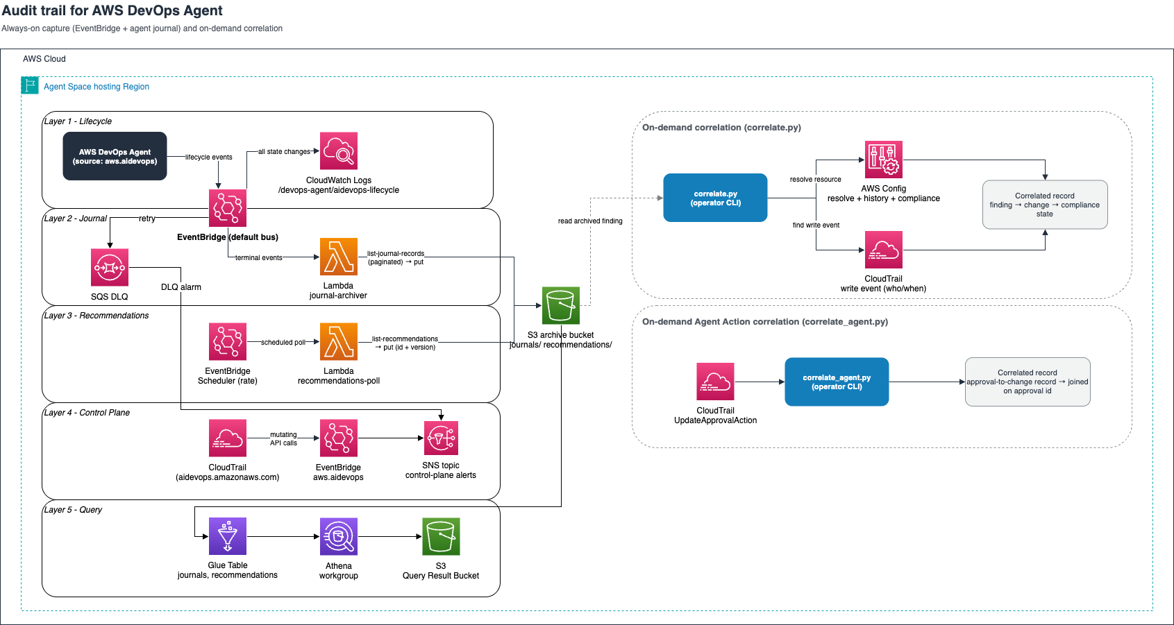
Five capture layers inside the Agent Space Region: lifecycle events to CloudWatch Logs, terminal events to a Lambda that archives journals to Amazon S3 with a dead-letter queue, a scheduled poll for recommendations, control-plane mutations to an SNS topic through Amazon EventBridge, and a Glue/Athena query layer. Two operator CLIs read the archive: correlate.py joins findings to AWS Config and CloudTrail, and correlate_agent.py joins agent actions to their approvals.

Figure 1: Reference architecture for auditing AWS DevOps Agent across five capture layers

Layer 1: Lifecycle capture. One Amazon EventBridge rule matching {"source":["aws.aidevops"]}, targeting an Amazon CloudWatch Logs (CloudWatch Logs) group directly. This durably records every lifecycle transition. Start here for operational visibility. If your primary goal is behavioral audit rather than operational visibility, deploy layer 2 alongside it.

Layer 2: Behavior capture. A second rule matches only terminal events and invokes a Lambda function. The function reads the execution_id from the event, calls list-journal-records, and writes the journal to Amazon S3. Subscribe to each terminal investigation and mitigation type. This is the layer that captures the agent’s decisions for the long term, including agent-based mitigations.

Layer 3: Recommendations snapshot. Because recommendations are generated on a schedule and have no event, capture them with an Amazon EventBridge Scheduler rule that invokes a Lambda function on a cadence (start daily). The function calls list-recommendations and writes each to Amazon S3, keyed on recommendation ID and version. It also calls list-goals in the same invocation, because a recommendation carries no field saying whether it is still current and the owning goal is the only thing that does. The journal captures what the agent found, and this layer captures what it advised and what you did about it.

Layer 4: Control-plane alerting. On your existing organization trail, alert on mutating aidevops.amazonaws.com events including UpdateApprovalAction, which is produced on elevated actions. This is your tripwire for changes to the agent itself.

Layer 5: Query. AWS Glue Data Catalog tables and an Amazon Athena (Athena) workgroup over the archived journals, recommendations, and goals.

Querying the archive: AWS Glue and Athena

The sample implementation overlays an AWS Glue Data Catalog and an Athena workgroup on the Amazon S3 archive. Three external tables cover the full archive. The journals table uses Athena partition projection, and Hive-partitioned by agent space and date:

s3://<amzn-s3-demo-archive-bucket>/journals/space=<agent-space-id>/dt=2026-07-28/<execution-id>.json

Volume of recommendations is low (tens to hundreds of objects), so a flat external table over the recommendations/ prefix is sufficient. Athena recurses subdirectories by default, picking up every versioned snapshot.

The result bucket has Amazon S3 Object Lock but Object Lock prevents Athena from managing its own query-result objects. The query layer deploys a dedicated results bucket with a seven-day lifecycle rule for ephemeral query outputs.

Access control

Use IAM to control access. Investigation journals contain the agent’s full reasoning about your infrastructure. Scope your IAM permissions on the Athena workgroup, AWS Glue database, and on the archive bucket itself since bucket read access bypasses Athena entirely. Scope all three to your audit and operations teams.

To find all findings from the past 7 days for a specific resource:

SELECT
  execution_id,
  event_time,
  task.title,
  record.content
FROM devops_agent_audit.journals
CROSS JOIN UNNEST(journal_records) AS t(record)
WHERE dt >= date_format(current_date - interval '7' day, '%Y-%m-%d')
  AND record.recordType IN ('finding', 'investigation_result')
  AND record.content LIKE '%sg-0123456789abcdef0%'
ORDER BY event_time DESC;

The Athena workgroup integrates with Amazon Quick or any business intelligence tool that speaks JDBC/ODBC. Additional examples are available in the sample repository.

Closing the loop: Correlating findings to actual changes

The capture layers record what the agent found and what it recommended. But did the recommended fix actually land? This requires connecting the agent’s output to the real infrastructure change that followed.

The sample implementation includes correlate.py, an on-demand operator CLI that takes an archived finding or recommendation, resolves the resource it references, and reports what changed, when, and who did it. The correlation is heuristic by looking at resource identity and a tight time window in minutes to produce reliable attribution. This is why the sample implementation pairs it with a deterministic engine for agent-initiated actions.

It works by pivoting through two services:

AWS Config resolves the resource identity by using select-resource-config, then pulls its configuration timeline from get-resource-config-history. This shows the before/after state of the resource around the time of the agent’s finding.
CloudTrail looks up the write event that caused the change: who called what API, from where, and when. This attributes the change to a principal.

The output is a correlated record: the agent found X, the resource changed from state A to state B, and that change was made by principal Y at time T.

Because CloudTrail indexes resources by different identifiers depending on the service, you require a strategy registry. Examples are in the following table:

Resource type	How CloudTrail indexes it	Lookup strategy
S3 bucket	Bucket name	By name
Lambda function	Function name	By name
Amazon Relational Database Service (Amazon RDS) instance/cluster	Full ARN (not the DB ID)	Build ARN from template
Amazon Elastic Compute Cloud (Amazon EC2) security group	Group ID as `ResourceName`	By name, with a resource-type scan as fallback

A naive “look up by resource name” works for Amazon S3 and Lambda but returns zero results for Amazon RDS (RDS). The strategy registry encodes the right ID per resource type.

Correlating agent actions

When an operator approves an elevated action, the service stamps the approval ID into the credential it mints, so the executed call carries that ID inside its own principal ARN (op.system.apr.<approvalId>). The sample implementation includes correlate_agent.py that uses this. Because the ID is present on both sides, the correlation is a join. The engine checks the executed call against the argumentPins the operator was shown at approval time, so you can prove the agent’s behavior.

.	`correlate.py`	`correlate_agent.py`
Pivots on	A resource the agent named	Agent’s approval ID
Correlation	heuristic	deterministic
Answers	Who changed?	Who approved, and did it match?
Dependency	`CloudTrail` and AWS Config	`CloudTrail`

Production considerations

Understand the data volume. Journal size scales with investigation complexity. As an example:

Scenario	Journal size	API calls (pagination)	Notes
Minimal (single-service, shallow investigation)	~65 KB	2–3 pages	Quick symptom to finding arc
Typical (multi-signal, 1–2 findings)	250–340 KB	65–106 calls	Typical investigations
Exhaustive (account-wide, high-priority)	~428 KB	150+ calls	Full cross-service correlation

At 100 investigations/month at 300 KB average, you are storing roughly 30 MB/month of journal data.

Concurrency per agent space. By default, you can run three concurrent investigations per agent space. Additional requests queue as PENDING_START and start when a slot opens. The archival pipeline is unaffected because each terminal event triggers its own Lambda invocation. Refer to the AWS DevOps Agent Quotas page for future updates.

Paginate the journal. The journal API is server-paginated: pass limit, follow nextToken until it’s empty. A real incident’s journal can span several pages. Always loop.

Design for at-least-once delivery. Amazon EventBridge can deliver an event more than once. Key the Amazon S3 object on execution_id so a redelivery overwrites rather than duplicates, and attach an Amazon Simple Queue Service (Amazon SQS) dead-letter queue (DLQ) so a dropped terminal event is not lost.

Deploy per AWS Region and per account. Events land on the default bus in each Agent Space’s hosting account and Region. If you run agent spaces in multiple accounts, you must aggregate events to a central monitoring account for unified visibility. Refer to Amazon EventBridge cross-account document for further details.

Make the archive immutable. Enable Amazon S3 Object Lock and versioning. The sample implementation defaults to GOVERNANCE mode but for stronger compliance posture, use COMPLIANCE mode.

Warning: COMPLIANCE mode is irreversible. After it’s set, no principal (including the account root user) can delete or modify locked objects before their retention period expires. The only way out is closing the AWS account, and Object Lock itself can’t be disabled once enabled. Choose COMPLIANCE mode deliberately. If you use GOVERNANCE mode, enable CloudTrail data events on the bucket.

Encrypt your data. The sample implementation uses SSE-S3. If your compliance framework requires you to control and audit decryption events, use SSE-KMS with customer managed key.

The full loop

Here’s what a complete audit trail looks like for a single incident through resolution.

Step 1: Investigation. The agent investigates a failing Lambda function, concludes its security group restricts necessary egress, and writes the finding to the journal. Layer 2 archives the journal to Amazon S3.

Step 2: Recommendation. On its goal cadence, the agent generates a recommendation: “Update the security group egress rules to allow…” Layer 3 polls and captures it as recommendations/rec-a1b2c3.../v1.json with status PROPOSED. A later poll captures v2.json as the status changes.

Step 3: Engineer applies the fix. An engineer runs the suggested command. AWS Config records the new configuration item, and CloudTrail records the API call with principal, source IP, and timestamp.

Step 4: Correlation.

$ python correlate.py --archive-bucket $BUCKET \
    --recommendation rec-a1b2c3d4-5e6f-7890-abcd-ef1234567890 \
    --window-hours 24

Recommendation: rec-a1b2c3d4-5e6f-7890-abcd-ef1234567890
Title:          Update the Lambda security group egress rules to allow API access
Status:         PROPOSED → UPDATE_IN_PROGRESS (v2)

AWS Config change detected:

  Resource:     AWS::EC2::SecurityGroup / sg-0123456789abcdef0
  Changed:      2026-07-23 08:45:54.105000-04:00
CloudTrail attribution:
  Event:        AuthorizeSecurityGroupEgress
  Principal:    arn:aws:iam::111122223333:user/jsmith
  Source IP:    203.0.113.10
  Time:         2026-07-23 08:44:33-04:00

Correlation:    OK Recommendation → AWS Config change → CloudTrail event aligned

The agent found the problem, recommended the fix, and you can prove who applied it and when.

Step 5: A new investigation. A later investigation examines the same Lambda function, still erroring. The agent compares new advice against advice it has already given, and that comparison is semantic. But it compares against the recommendations currently attached to the goal, not against everything it has ever advised, and when the comparison is uncertain it keeps the two separate. Older advice drops out of that comparison set over time. Because you archived every recommendation and every finding with their resource identifiers, you can now compare across the full history:

$ python correlate.py --archive-bucket $BUCKET \
    --finding  exe-ops1-0f1e2d3c-4b5a-6978-8796-a5b4c3d2e1f0 \
    --check-prior-recommendations

Resource:       AWS::EC2::SecurityGroup /  sg-0123456789abcdef0

Prior recommendations referencing this resource:
   rec-a1b2c3d4-5e6f-7890-abcd-ef1234567890 (v2, UPDATE_IN_PROGRESS):
    "Update the security group egress rules..."
   rec-b2c3d4e5-6f70-8901-bcde-f01234567890 (v1, PROPOSED):
    "Update the security group egress rules..."

! This finding may be a consequence of recommendation(s): rec-a1b2c3d4-5e6f-7890-abcd-ef1234567890, rec-b2c3d4e5-6f70-8901-bcde-f01234567890
Last change to this resource (CloudTrail): Event: AuthorizeSecurityGroupEgress Principal: arn:aws:iam::111122223333:user/jsmith Source IP: 203.0.113.10 Time: 2026-07-23 08:44:33-04:00

The archive diagnosed the cause of the cause. Two recommendations, raised separately, on one resource, in one view. The agent’s own comparison covers the advice currently attached to the goal. The archive covers all of it. That is the feedback loop the audit trail adds.

Agent Actions changes Step 3’s actor, and the agent applies the fix directly. In the recommendation path, the human runs the command. In the elevated-action path, the human approves a specific call, and the agent executes it under a single-use session. correlate_agent.py uses a single-use session named for the approval (op.system.apr.<approvalId>), with invokedBy: aidevops.amazonaws.com rather than a time-window heuristic.

Operating the pipeline: Common failures

Always design for failure. Here are some common failures and how to detect and recover.

Failure	Symptom	Detection	Recovery
Lambda timeout	No archive in Amazon S3. Event in DLQ	DLQ `ApproximateNumberOfMessagesVisible` alarm	Increase timeout above the 2-minute default. Replay DLQ message which is idempotent on the `execution_id` key
Missed recommendation poll	Gap in `recommendations/` prefix with a version number skipped	Periodic reconciliation: compare Amazon S3 keys against `list-recommendations` response	Re-run poll Lambda manually (idempotent)
Amazon EventBridge delivery failure	Missing lifecycle event in Layer 1 logs	Layer 2 archive exists without matching Layer 1 log entry	No data loss since journal already archived. Gap is in lifecycle visibility only
Amazon S3 write failure	Lambda errors spike. DLQ grows	Lambda error rate metric and DLQ alarm	Fix IAM/bucket policy. Replay DLQ (all messages are idempotent)
AWS Config recorder stopped	`correlate.py` returns no configuration history	AWS Config recorder status alarm	Re-enable recorder. Note: historical gap is permanent for the stopped period
Journal API throttled	Partial archive. Lambda retries exhaust timeout	Lambda error logs showing throttling exceptions	Implement exponential backoff in the pagination loop. Increase timeout
Approval recorded but not executing	Approval exists in CloudTrail with no corresponding write	Join approvals to execution on the approval ID	None needed

The highest value alarm is on the DLQ message count. A non-empty DLQ means a terminal event triggered, but the journal was not archived. Terminal events aren’t re-emitted, and the DLQ retains messages for 14 days. After that, the record is lost. The sample implementation ships this alarm at a threshold of 1, wired to an Amazon Simple Notification Service topic.

Run a reconciliation check weekly or monthly. Compare the execution_id values in the Layer 1 lifecycle log against the set of keys in the Amazon S3 journals/ prefix. Any ID in the logs but not in Amazon S3 represents a missed archive.

Limitations

Automated correlation – The current design requires a human to run correlate.py. Extend to a Lambda function that triggers on each new journal archive, cross-references the finding’s resource identifiers against the recommendations table, and alerts when a new finding touches a resource that was the subject of a prior recommendation.

Schema evolution – The Athena table definitions depend on the journal’s recordType values and content structure. If new record types appear, queries can return incomplete results without raising an error. Monitor for unknown recordType values. A query that returns zero findings for a week of active investigations is a signal that the schema moved.

Conclusion

Adopting an autonomous agent is a trust decision, and trust needs evidence. AWS DevOps Agent gives you the raw material: a journal of its reasoning, a real-time lifecycle event stream, a control-plane audit in CloudTrail, and an action boundary you can read straight from IAM. The pattern in this post assembles those into a durable, low-maintenance audit trail using services you already run.

The archive is more than compliance paperwork. With a persistent record of every finding and every recommendation, you can correlate across investigations and recommendations the agent no longer has in view, and against the present state of your infrastructure. That feedback loop is the difference between trusting the agent and understanding it.

Start with Layer 1. A single Amazon EventBridge rule to a log group gives you visibility into every investigation within minutes. Add the journal-archiving Lambda when you are ready to retain the agent’s decisions for the long term. Add the correlation layer when you want to prove that recommendations were acted on and catch the ones that created new problems.

Clone the sample repo to get started. It covers prerequisites, deploy steps, codebases, and teardown instruction. If you want the agent’s mitigations to become code, Automated incident remediation with AWS DevOps Agent and Kiro CLI builds a pipeline.

About the authors

How Meta Glasses Are Fueling the Anti-Surveillance Sentiment

2026-09-28 The Atlantic

Post Syndicated from The Atlantic original https://www.youtube.com/shorts/674xQ_hmkCs

Isolate email reputation in Amazon SES Mail Manager with tenant management

2026-09-28 Abilashkumar P C

Post Syndicated from Abilashkumar P C original https://aws.amazon.com/blogs/messaging-and-targeting/isolate-email-reputation-in-amazon-ses-mail-manager-with-tenant-management/

When AnyCompany’s new IT outsource team misconfigured the email settings on 200 of the company’s multifunction printer/scanners, it had two bad outcomes. First, nobody received their scanned documents in their inboxes. Somewhat predictably, many users rescanned the same documents multiple times before creating support tickets. Second, the misconfiguration along with the multiple failed attempts resulted in a “bounce storm” that was quickly reported by a major email service provider, but unfortunately ignored by the IT team.

Within 48 hours, the bounce rate crossed the provider’s threshold. The company’s entire Amazon Simple Email Service (Amazon SES) account lost its sending reputation. Password resets, order confirmations, and service notifications from every business unit on the account started landing in spam or failing to deliver. The damage spread because every sender on the account, from the mission-critical billing system to the misconfigured printers, shared the same reputation score.

This is a preventable problem. With Amazon SES tenant management you can isolate email reputation per tenant inside a single account so one misbehaving sender cannot affect the rest. If you use Amazon SES Mail Manager for Simple Mail Transfer Protocol (SMTP) filtering, routing, archiving, or relay, you can activate tenant isolation. To do so, tag each message with the X-SES-TENANT header in your Mail Manager rule set. In this post, you will compare five architectural patterns for applying the X-SES-TENANT header, from static per-tenant endpoints to AWS Lambda driven runtime resolution.

This post complements Isolate email suppression per tenant with Amazon SES. That post explains how tenant-level suppression lists prevent cross-tenant bounce and complaint contamination, which is the “what happens after the message is tagged” story. This post focuses on the upstream problem: how to get the X-SES-TENANT tag onto messages when your senders are legacy appliances, printers, or applications that can’t set custom MIME headers. Together, the two posts cover the full tenant isolation pipeline, from tagging through delivery and suppression.

This post provides architectural guidance. For step-by-step implementation, refer to the Amazon SES documentation.

How SES tenant isolation works

Amazon SES tenant management isolates reputation per tenant inside a single Amazon SES account. Each tenant acts as a container organized around sending identities, configuration sets, and the resulting reputation metrics. Amazon SES attributes bounces, complaints, and Trust and Safety signals to the tenant, not the account, so a deliverability issue in one tenant doesn’t affect the others.

A critical benefit of tenant isolation: when one tenant’s reputation degrades beyond a threshold, Amazon SES can pause sending for that tenant only. Other tenants continue delivering normally. Without tenant isolation, a reputation issue affects the entire account. This pause-and-contain mechanism is one of the strongest reasons to adopt tenant management, especially for accounts with diverse sender types.

You associate a message with a tenant by passing the TenantName parameter on the Amazon SES API v2 SendEmail operation, or by adding an X-SES-TENANT Multipurpose Internet Mail Extensions (MIME) header to an SMTP message. For a detailed walkthrough of tenant management concepts, including identity ownership, the ses:TenantName AWS Identity and Access Management (IAM) condition key, and tenant-level suppression lists, see Improve email deliverability with tenant management in Amazon SES.

How Mail Manager works

Mail Manager processes inbound and outbound SMTP traffic through a pipeline of three components:

Ingress endpoint: an authenticated SMTP endpoint that accepts connections from your senders. Mail Manager ingress endpoints handle SMTP only, not the Amazon SES API.
Traffic policy: filters connections based on sender attributes (IP, TLS version, authentication) before messages reach rule processing.
Rule set: an ordered list of rules. Each rule has conditions (match on envelope sender, recipient, source IP, or header values) and actions (Add header, Write to S3, Invoke Lambda, Send to internet, SMTP relay, Drop).

The “Add header” rule action is what makes tenant isolation possible for legacy senders: it injects the X-SES-TENANT SMTP header before the “Send to internet” action hands the message to Amazon SES for delivery.

With the “Add header” rule action inserted before the “Send to internet” action in the same rule, Mail Manager effectively tags the message with the SMTP header that defines the tenant. When Amazon SES processes the send, it reads the X-SES-TENANT header and attributes the message to the corresponding tenant.

Amazon SES performs tenant attribution only during send processing. A Send to internet action, or a Lambda function that calls SendEmail with the TenantName parameter or X-SES-TENANT header, activates tenant management. An SMTP relay action forwards to a third-party SMTP server (Google Workspace, Microsoft 365, or on-premises mail), so Amazon SES doesn’t process the send and tenant attribution doesn’t apply. Write to S3 and Drop don’t hand messages to Amazon SES, so they don’t activate tenant management either. This post describes flows that include a Send to internet action or a Lambda function calling SendEmail.

Understanding the outbound email flow

An outbound message flows from the SMTP client to the Mail Manager ingress endpoint, passes through the traffic policy and rule set, then routes through Amazon SES to the internet.

Figure 1: Outbound email flow from an SMTP client through Mail Manager to Amazon SES

Compare the patterns

Before diving into each pattern, use this table to identify which one fits your workload. You can then read only the pattern section that applies, or read all five for the full picture.

Consideration	Pattern 1	Pattern 2	Pattern 3	Pattern 4	Pattern 5
Works for legacy and appliance senders	—	Yes	Yes	Yes	Yes
Retrieve tenant from static value	Yes	Yes	Yes	Yes	Yes
Retrieve tenant from source IP or sender condition	—	Yes	Yes	Yes	Yes
Retrieve tenant from runtime lookup or body inspection	—	—	—	Yes	Yes
Records Send in Mail Manager log	Yes	Yes	Yes	—	—
Tenants per Region	Up to 10,000	~50	400 (per-tenant Send) or 1,560 (chained)	Up to 10,000	Up to 10,000

One difference cuts across the patterns: where the tenant mapping lives determines what it takes to change it. Patterns 2 and 3 hold the mapping in rule-set configuration, so adding or removing a tenant is a rule-set edit and deployment (a control-plane change, not a data change). Patterns 4 and 5 resolve the tenant from a runtime source such as a database, so onboarding or offboarding a tenant is a data update that takes effect without a deployment. In Pattern 1, the sender supplies the tenant, so there’s no mapping to maintain in Mail Manager at all.

Pattern 1: The SMTP sender sets the header before Mail Manager

Pattern 1, where the SMTP sender sets the X-SES-TENANT header before the message reaches the Mail Manager ingress endpoint

Figure 2: Pattern 1, where the SMTP sender sets the tenant header before Mail Manager

If the SMTP sender (a backend service, internal tool, or any application that can add a custom MIME header) sets X-SES-TENANT on the message before connecting to the Mail Manager ingress endpoint, the message arrives pre-tagged. The rule set only needs a Send to internet action.

Pattern 1 fits customers who already use Mail Manager for filtering, archiving, or compliance and whose sending applications can add one header at send time. You keep Mail Manager gateway capabilities without adding Add header or conditional logic to the rule set.

Pattern 2: Mail Manager adds a static header with Add header

Pattern 2, where a Mail Manager rule adds a static X-SES-TENANT header and then sends the message to the internet

Figure 3: Pattern 2, where a Mail Manager rule adds a static tenant header

A rule with Add header followed by Send to internet attaches a fixed tenant value to each message. This pattern fits a one-tenant-per-endpoint model: provision one authenticated ingress endpoint per tenant, give each tenant its own SMTP credentials, and attach a rule set that injects the tenant value.

For example, an enterprise provisions one endpoint for facilities-printer notifications and a second for corporate alerts. The Send to internet action’s IAM role grants permission only to that tenant’s Amazon SES identities, preventing a misrouted client from sending as another tenant.

You can group tenants behind one endpoint when they share a sending configuration. The header value and IAM scope live in the rule-set configuration, and no code runs at send time.

Pattern 3: Mail Manager derives the header from rule conditions

If multiple tenants share an endpoint but have stable distinguishing attributes (like source IP), one rule set handles each of them. Rule conditions match on envelope properties, and matching rules run an Add header action that sets X-SES-TENANT to the correct value.

Pattern 3, where Mail Manager derives the X-SES-TENANT header value from rule conditions before sending to the internet

Figure 4: Pattern 3, where Mail Manager derives the tenant header from rule conditions

Mail Manager rule sets allow 40 rules with up to 10 conditions and 10 actions per rule, but caps Send to internet and SMTP relay actions at 10 per rule set (counting every occurrence). One Send to internet per tenant rule tops out at 10 tenants.

To support more tenants, separate header-setting from delivery:

Rules 1 to 39: Each matches a distinguishing condition and runs a single Add header action.
Rule 40: A catch-all with no conditions and a single Send to internet action.

Each message matches at most one header-setting rule, picks up its tenant header, and passes through the catch-all. The effective ceiling is now 39 tenants per rule set with one Send to internet action and one IAM role.

Scale limits of Pattern 3

Pattern 3’s ceiling depends on how you structure the rule set. Two cases:

Case A: Chained structure (39 Add header rules + 1 Send to internet rule): Each rule set uses one Send to internet action, so the 10-action cap isn’t binding. Capacity is 39 tenants per rule set × 40 rule sets per Region = 1,560 tenants per Region.

Case B: Per-tenant Send to internet (each tenant rule has its own Send action): The 10-action cap binds at 10 tenants per rule set. Capacity is 10 tenants per rule set × 40 rule sets per Region = 400 tenants per Region.

The two cases trade off scale against IAM scoping. Case A shares one IAM role across all tenants in the rule set. Case B gives each tenant its own IAM role at the cost of 4× fewer tenants.

Amazon SES supports up to 10,000 tenants per account (adjustable). Workloads that exceed a few hundred tenants, or need runtime tenant changes, can use Pattern 4 or Pattern 5.

Pattern 4: Mail Manager calls Lambda for runtime tenant resolution

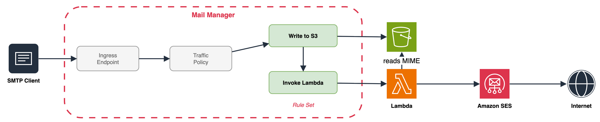
Pattern 4, where Mail Manager writes the message to Amazon S3 and invokes a Lambda function that resolves the tenant and delivers through Amazon SES

Figure 5: Pattern 4, where Mail Manager invokes a Lambda function for runtime tenant resolution

Some tenant values require runtime logic, such as a database lookup on the sender IP, an external policy service, or content inspection. For these cases, the Mail Manager Invoke Lambda action runs a Lambda function inside the rule chain.

The Lambda event carries only metadata (headers, envelope sender, recipients, verdicts), not the MIME body. The function also can’t modify the message for downstream actions. Lambda must therefore handle delivery.

The rule writes the raw MIME to Amazon S3 with Write to S3, then invokes the Lambda function with the message ID. The function fetches the object and determines the tenant through the runtime logic your workload requires. That logic might be a database lookup (for example, an Amazon DynamoDB query), a call to an external policy service, or inspection of the message body. It then calls the Amazon SES API v2 SendEmail operation, passing the resolved tenant in the TenantName parameter. Delivery permissions live on the function’s execution role, which carries the ses:TenantName condition key.

The Lambda function is yours to build and maintain. This gives you full control over the tenant resolution logic and everything downstream (retries, dead-letter queues, observability), but it also means you own the operational overhead: code updates, monitoring, and cost management.

Mail Manager can invoke the function synchronously or asynchronously. Synchronous invocation (REQUEST_RESPONSE) keeps Lambda in Mail Manager’s critical path: Mail Manager waits up to 30 seconds for the function to return, and retries on failure. Asynchronous invocation (EVENT) hands control to Lambda instead, so Mail Manager invokes the function and moves on. There are no additional Mail Manager charges for the Lambda invocation beyond standard Lambda pricing.

Pattern 5: Mail Manager stages to Amazon S3, Lambda delivers asynchronously

Pattern 5, where an Amazon S3 event triggers a Lambda function that delivers the message through Amazon SES

Figure 6: Pattern 5, where an Amazon S3 event triggers a Lambda function that delivers the message

In Pattern 4, Mail Manager invokes the function directly through the Invoke Lambda rule action. Pattern 5 removes that direct invocation: the Mail Manager rule ends at Write to S3, and an Amazon S3 event notification triggers the Lambda function instead. Mail Manager’s work finishes at the write, and delivery becomes fully event-driven.

The rule set has two actions: write the raw MIME to Amazon S3, followed by an explicit Drop action. The Drop action prevents accidental duplicate delivery if a Send to internet action is inadvertently added to the rule later. The Lambda function handles delivery through the Amazon SES API, so Mail Manager’s job ends at writing the MIME to Amazon S3. The Amazon S3 event routes to the function directly or through Amazon Simple Queue Service (Amazon SQS) or Amazon EventBridge for fan-out and back-pressure.

The function reads the object, performs the tenant lookup, and calls SendEmail with the TenantName parameter. The Mail Manager critical path is minimal, and Lambda retries use the Lambda retry model with dead-letter queue support. The same Amazon S3 object fans out to multiple consumers (delivery, analytics) without changing the Mail Manager rule.

The Lambda function is yours to build and maintain. The upside is full control over the function and everything after it: tenant resolution logic, retries, dead-letter queues, and observability. The tradeoff is cost and upkeep, since you own code updates, monitoring, and operational overhead.

The other tradeoff is less visibility. After Write to S3, the Mail Manager log no longer records the delivery outcome.

Secure tenant attribution with IAM

Regardless of which pattern sets the X-SES-TENANT header, the Send to internet action’s IAM role should enforce tenant boundaries. Scope the IAM role with a Condition element that includes the ses:TenantName condition key.

Example IAM policy:

{
  "Version": "2012-10-17",
  "Statement": [
    {
      "Effect": "Allow",
      "Action": "ses:SendEmail",
      "Resource": "*",
      "Condition": {
        "StringEquals": {
          "ses:TenantName": "facilities-printers"
        }
      }
    }
  ]
}

This policy allows the role to send email only when the message is attributed to the facilities-printers tenant. Messages tagged with any other tenant value, or messages with no tenant header, are denied.

In Pattern 1, the sender sets the header, the IAM role on the Send to internet action validates that the claimed tenant matches the role’s permissions. In Pattern 2, the Add header action sets a fixed value, and the IAM role confirms the header matches the expected tenant for that endpoint. In Pattern 3 with a chained structure, a single Send to internet action services all tenants. Scope its role to the set of valid tenant names so untagged messages (those matching no Add header rule) fail authorization. For Patterns 4 and 5, the Lambda function’s execution role carries the ses:TenantName condition key, providing the same enforcement at the API call level.

Paused tenants

Each of the five patterns handles paused tenants the same way. When Amazon SES pauses a tenant (through a reputation policy or manually), sends for that tenant fail with a rejection error. Other tenants keep delivering. The failure surfaces depending on the pattern:

Patterns 1 to 3: Mail Manager records the rejection in the rule set log.
Patterns 4 and 5: The rejection surfaces in the Lambda function’s Amazon CloudWatch Logs.
Patterns 1 to 5: Amazon SES publishes tenant status changes to Amazon EventBridge (such as Sending Status Disabled).

Mail Manager won’t re-route or retry a paused tenant send. Graceful handling (queueing, failover, notification) belongs in the Lambda function in Patterns 4 and 5.

Observability

Observability for these patterns draws on three sources, each answering a different question:

Mail Manager vended log: which rule actions ran, and whether Amazon SES accepted the message from a Send to internet action. Mail Manager delivers this log to a destination you configure: Amazon CloudWatch Logs, Amazon S3, or Amazon Data Firehose. Query CloudWatch Logs with CloudWatch Logs Insights, or query Amazon S3 with Amazon Athena to surface IAM denials, configuration errors, and throttling.

Amazon SES event publishing: the final delivery outcome (delivered, bounced, or complaint), routed through a configuration set. This applies to every pattern.

Lambda Amazon CloudWatch Logs: for Patterns 4 and 5, where delivery runs inside the Lambda function, the acceptance result and any application errors.

To trace a message end to end, correlate these sources. For Patterns 1 to 3, the Mail Manager log and Amazon SES event publishing cover the flow. For Patterns 4 and 5, add the Lambda function’s CloudWatch Logs, since the Mail Manager log ends at Invoke Lambda (Pattern 4) or Write to S3 (Pattern 5).

Limits that shape the architecture

Review the Amazon SES Mail Manager service quotas before committing to a pattern. These quotas most often drive your pattern choice:

Resource	Default	Where it matters
Maximum message size (SMTP ingress)	40 MB	Patterns 1 to 5
Authenticated ingress endpoints per Region	50	Pattern 2 per-tenant endpoints
Rule sets per Region	40	Pattern 2, Pattern 3 partitioning
Rules per rule set	40	Pattern 3
Send to internet action per rule set	10	Pattern 3 tightest constraint
Actions per rule	10
Conditions per rule	10
Addresses per address list	100,000	Pattern 3 consolidation
Tenants per account (Amazon SES)	10,000 (adjustable)	Patterns 4 and 5 ceiling
Lambda concurrent executions per Region	1,000 (adjustable)	Patterns 4 and 5 throughput ceiling
Lambda timeout (Mail Manager InvokeLambda)	30 seconds	Pattern 4 synchronous path
S3 event notification destinations per prefix	1 (use Amazon EventBridge for fan-out)	Pattern 5 fan-out design
Lambda invocation payload (synchronous)	6 MB	Pattern 4 metadata-only (body in S3)
Sending quota per 24 hours (Amazon SES)	200 in sandbox (adjustable in production)	Patterns 1 to 5
Maximum send rate (Amazon SES)	1 message/second in sandbox (adjustable in production)	Patterns 1 to 5

Conclusion

The five patterns in this post show how to architect tenant tagging, whether through static endpoints, rule-set headers, or runtime resolution, so you can choose the approach that fits your workload.

Next steps

Create your first ingress endpoint and rule set in the Mail Manager console.
Create your first tenant.
Review the tenant management page.
Review the Amazon SES product detail page for pricing and Regional availability.
Read the Amazon SES Mail Manager documentation.
Learn how tenant-level suppression lists prevent cross-tenant contamination in Isolate email suppression per tenant with Amazon SES.

About the authors

Getting started with Apache Iceberg write support in Amazon Redshift – Part 3

2026-09-28 Raghu Kuppala

Post Syndicated from Raghu Kuppala original https://aws.amazon.com/blogs/big-data/getting-started-with-apache-iceberg-write-support-in-amazon-redshift-part-3/

Production data is always evolving. Tables gain and lose columns, outgrow their data types, and get re-partitioned as query patterns shift. Multiple engines often need to read the same data. These changes used to mean expensive data rewrites or rebuilt pipelines. Apache Iceberg makes them metadata-only operations, and Amazon Redshift now supports evolving schemas and partitioning layouts through ALTER statements, with no data rewrites and no pipeline rebuilds. You can also create AWS Lake Formation resource links in the catalog of Amazon S3 Tables, a capability of Amazon Simple Storage Service (Amazon S3), for centralized cross-engine governance.

In Part 1, you created Apache Iceberg tables and wrote data directly from Amazon Redshift to your data lake, setting up external schemas, creating tables in both Amazon Simple Storage Service (Amazon S3) and Amazon S3 Tables, and performing INSERT operations with full ACID (Atomicity, Consistency, Isolation, Durability) compliance. In Part 2, you performed DELETE, UPDATE, and MERGE operations to modify data at the row level and synchronize staging and production tables.

In this post, you use the customer and orders datasets from the previous posts to evolve Iceberg table schemas and partitioning with ALTER operations. You also create an AWS Lake Formation resource link in the S3 Tables catalog to share tables with other analytics engines under a single, centralized permission model.

Solution overview

This solution demonstrates ALTER operations for Apache Iceberg tables in Amazon Redshift and Lake Formation resource link creation for the S3 Tables catalog. The walkthrough includes the following key operations:

ALTER TABLE RENAME COLUMN – Rename existing columns without changing data types or partition specs.
ALTER TABLE ADD/DROP COLUMN – Add new columns or remove existing columns as metadata-only operations.
ALTER TABLE ALTER COLUMN – Widen column data types (for example, INT to BIGINT) without rewriting data.
ALTER TABLE SET TABLE PROPERTIES – Change compression type for future writes.
ALTER TABLE ADD/DROP/REPLACE PARTITION FIELD – Evolve partition specs without re-partitioning existing data.
Lake Formation resource link – Create a resource link in the S3 Tables catalog for centralized access governance.

The following diagram shows the end-to-end architecture:

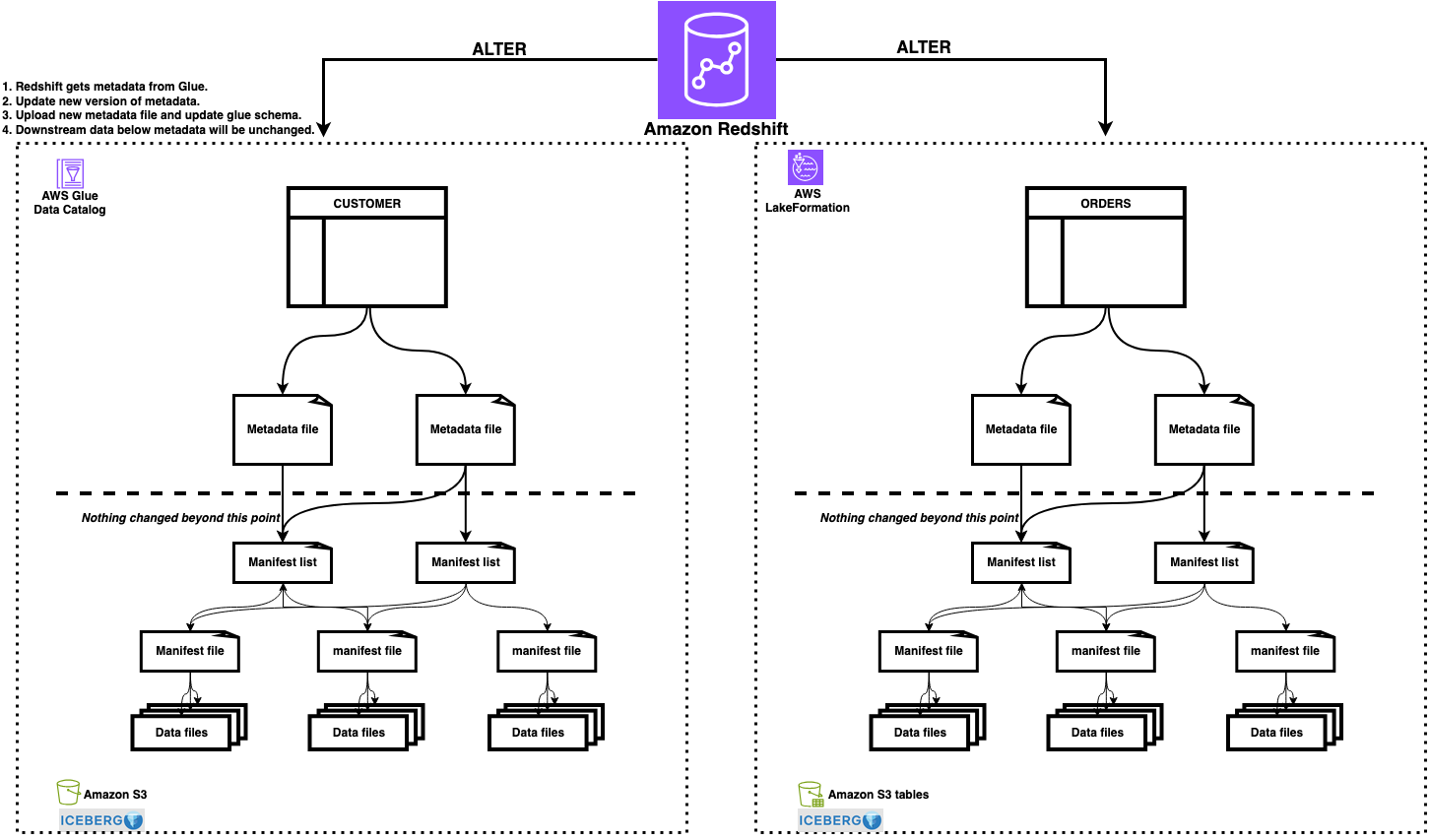
Architecture diagram of Amazon Redshift running ALTER operations on Iceberg tables in S3 Tables, with Lake Formation resource links providing access from Amazon Athena and other engines

Figure 1: Architecture showing Amazon Redshift performing ALTER operations on Iceberg tables in S3 Tables, with Lake Formation resource links providing access from Amazon Athena and other engines

Prerequisites

Complete the setup from Part 1 and Part 2, including:

An Amazon Redshift data warehouse (provisioned or Serverless) on patch 201 or higher.
The AWS Identity and Access Management (IAM) role (RedshifticebergRole) with permissions for Amazon S3, AWS Glue Data Catalog, and Lake Formation.
The customer table in a standard Amazon S3 bucket (AWS Glue catalog: customer_db).
The orders table in an Amazon S3 table bucket (iceberg-write-blog@s3tablescatalog).
Access to an IAM role that is a Lake Formation data lake administrator.
AWS Glue Data Catalog integrated with S3 Tables (s3tablescatalog exists).

Schema evolution with ALTER TABLE

With ALTER TABLE, you can change Iceberg table definitions, including schema, partition specs, and properties, without rewriting stored data. Each operation updates only metadata. The table structure changes instantly while existing data files remain untouched. This helps make schema evolution, partition adjustments, and property updates safe to run on production tables.

Add a column

You can add a new column to an Iceberg table using ALTER TABLE. Each new column is added with a unique field ID that Iceberg uses for column tracking across schema evolution. Existing rows return NULL for the newly added column.

Verify the current schema:

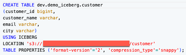
SHOW TABLE dev.demo_iceberg.customer;

SHOW TABLE output listing the current columns of the customer table

Figure 2: SHOW TABLE output showing the current customer table schema

Add the column:

-- Add a loyalty_tier column to the customer table
ALTER TABLE dev.demo_iceberg.customer
ADD COLUMN loyalty_tier VARCHAR;

Verify the schema change:

SHOW TABLE dev.demo_iceberg.customer;

SHOW TABLE output showing the new loyalty_tier column added to the customer schema

Figure 3: SHOW TABLE output showing the loyalty_tier column added to the schema

The following output shows the new loyalty_tier column as NULL for existing rows:

SELECT customer_id, customer_name, city, loyalty_tier
FROM dev.demo_iceberg.customer
ORDER BY customer_id;

Query results showing loyalty_tier as NULL for existing customer rows

Figure 4: Query results showing loyalty_tier as NULL for existing rows

Populate the new column by aggregating order totals from the orders table in S3 Tables:

-- Set loyalty_tier based on total spend from orders
UPDATE dev.demo_iceberg.customer
SET loyalty_tier = CASE
WHEN a.total_spend > 300 THEN 'Gold'
ELSE 'Silver'
END
FROM (
SELECT customer_id, SUM(total_order_amt) AS total_spend
FROM "iceberg-write-blog@s3tablescatalog".iceberg_write_namespace.orders
GROUP BY customer_id
) AS a
WHERE dev.demo_iceberg.customer.customer_id = a.customer_id;

The following output shows customer loyalty tiers after the update:

SELECT customer_id, customer_name, loyalty_tier
FROM dev.demo_iceberg.customer
ORDER BY customer_id;

Figure 5: Customer table showing Gold and Silver loyalty tiers

Note: Customer IDs 11, 13, and 15 show NULL for loyalty_tier because they have no matching orders in the orders table.

Drop a column

Remove columns that are no longer needed. The column is removed from the current schema, but data in existing files remains untouched and simply becomes invisible to queries.

Verify the current schema:

SHOW TABLE dev.demo_iceberg.customer;

SHOW TABLE output showing the customer schema before dropping loyalty_tier

Figure 6: SHOW TABLE output showing the current customer table schema before dropping loyalty_tier

Drop the column:

-- Drop the loyalty_tier column
ALTER TABLE dev.demo_iceberg.customer
DROP COLUMN loyalty_tier;

Verify the schema change:

SHOW TABLE dev.demo_iceberg.customer;

SHOW TABLE output showing the customer schema after loyalty_tier is dropped

Figure 7: SHOW TABLE output showing the customer table schema after loyalty_tier is dropped

Verify the column is dropped:

SELECT * FROM dev.demo_iceberg.customer
ORDER BY customer_id;

Query results confirming the loyalty_tier column no longer appears

Figure 8: Query results confirming the loyalty_tier column has been dropped

Note: To drop a column used in the current partition spec, first drop or replace the partition field, then drop the column.

Rename a column

Rename a column without affecting data types or partition specs:

-- Rename city to location
ALTER TABLE dev.demo_iceberg.customer
RENAME COLUMN city TO location;

The following output confirms the column has been renamed to location:

SELECT customer_id, customer_name, location
FROM dev.demo_iceberg.customer
ORDER BY customer_id;

Query results showing the city column renamed to location

Figure 9: Query results showing the renamed column location

Widen a column type

Widen a column’s data type without rewriting data. This is useful when your data outgrows the original precision, for example when order amounts exceed the original decimal range.

Verify the current column type:

SHOW TABLE "iceberg-write-blog@s3tablescatalog".iceberg_write_namespace.orders;

Figure 10: SHOW TABLE output showing total_order_amt as DECIMAL(10,2)

Now run the ALTER to widen the column:

-- Widen total_order_amt to support larger order values
ALTER TABLE "iceberg-write-blog@s3tablescatalog".iceberg_write_namespace.orders
ALTER COLUMN total_order_amt TYPE DECIMAL(18,2);

Verify the updated column type:

SHOW TABLE "iceberg-write-blog@s3tablescatalog".iceberg_write_namespace.orders;

SHOW TABLE output showing total_order_amt widened to DECIMAL(18,2)

Figure 11: SHOW TABLE output confirming total_order_amt widened to DECIMAL(18,2)

Note: Amazon Redshift supports safe type promotions (for example, INT to BIGINT, FLOAT to DOUBLE, DECIMAL(10,2) to DECIMAL(18,2)). Plan column types accordingly for future growth.

Set table properties

Change the compression type for future writes:

Verify the current compression type:

SHOW TABLE "iceberg-write-blog@s3tablescatalog".iceberg_write_namespace.orders;

SHOW TABLE output showing the orders table compression type before the change

Figure 12: SHOW TABLE output showing the current compression type before the update

Now run the ALTER to change the compression type:

-- Switch to zstd compression for better ratios
ALTER TABLE "iceberg-write-blog@s3tablescatalog".iceberg_write_namespace.orders
SET TABLE PROPERTIES ('compression_type'='zstd');

The following SHOW TABLE output confirms the updated compression setting:

SHOW TABLE "iceberg-write-blog@s3tablescatalog".iceberg_write_namespace.orders;

Figure 13: SHOW TABLE output showing compression_type set to zstd

Note: This affects only future writes. Existing data files retain their original compression.

Partition evolution

A powerful feature of Iceberg is partition evolution, the ability to change how a table is partitioned without rewriting existing data. Amazon Redshift writes new data with the updated partition scheme, while existing data remains in the old layout. Query engines handle both layouts transparently.

Adding a partition field

The orders table from Part 1 is partitioned by DAY(order_date). Add an additional bucket partition to distribute data across hash buckets:

Verify the current partition spec:

SHOW TABLE "iceberg-write-blog@s3tablescatalog".iceberg_write_namespace.orders;

SHOW TABLE output showing the orders partition spec before adding a field

Figure 14: SHOW TABLE output showing the current partition spec before adding a partition field

Add the partition field:

-- Add bucket partitioning on customer_id
ALTER TABLE "iceberg-write-blog@s3tablescatalog".iceberg_write_namespace.orders
ADD PARTITION FIELD bucket(16, customer_id);

After this change, new data is partitioned by both DAY(order_date) and bucket(16, customer_id), while existing data remains in the original day-only layout.

Verify the updated spec:

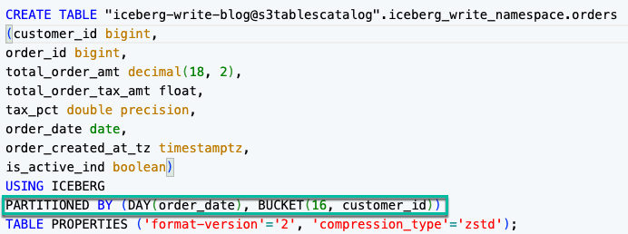
SHOW TABLE "iceberg-write-blog@s3tablescatalog".iceberg_write_namespace.orders;

SHOW TABLE output showing partition spec with DAY(order_date) and bucket(16, customer_id)

Figure 15: SHOW TABLE output showing the updated partition spec with DAY(order_date) and bucket(16, customer_id)

Replacing a partition field

Instead of separately dropping and adding, use REPLACE PARTITION FIELD as a single atomic operation. This is the recommended approach when swapping one transform for another on the same source column, because it makes the intent explicit and avoids a transient state where the table is unpartitioned between operations.

Verify the current partition spec:

SHOW TABLE "iceberg-write-blog@s3tablescatalog".iceberg_write_namespace.orders;

SHOW TABLE output showing the current DAY(order_date) partition spec

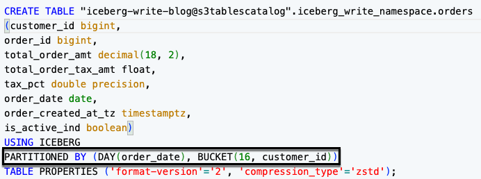
Figure 16: SHOW TABLE output showing the current partition spec with DAY(order_date) and bucket(16, customer_id)

Replace the partition field:

-- Replace daily partitioning with monthly
ALTER TABLE "iceberg-write-blog@s3tablescatalog".iceberg_write_namespace.orders
REPLACE PARTITION FIELD DAY(order_date) WITH MONTH(order_date);

After this change:

Existing data remains in day-based partition folders.
Amazon Redshift writes new data into month-based partition folders.
The query engine reads both layouts transparently.

Confirm the new partition spec:

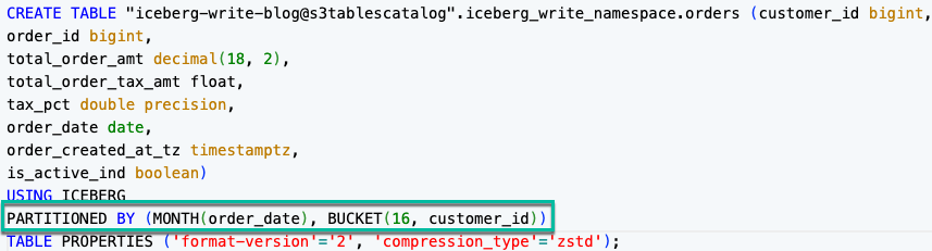
SHOW TABLE "iceberg-write-blog@s3tablescatalog".iceberg_write_namespace.orders;

Figure 17: SHOW TABLE output confirming the partition field replaced with MONTH(order_date)

Insert new data and verify that both partition layouts are queryable:

-- New data follows monthly partitioning
INSERT INTO "iceberg-write-blog@s3tablescatalog".iceberg_write_namespace.orders
(order_date, order_id, customer_id, total_order_amt, total_order_tax_amt,
tax_pct, order_created_at_tz, is_active_ind)
VALUES
('2025-01-15', 1018, 3, 210.00, 16.80, 0.08, '2025-01-15 09:00:00-06:00', true);
-- Query spans both old (daily) and new (monthly) layouts transparently
SELECT order_id, order_date, total_order_amt
FROM "iceberg-write-blog@s3tablescatalog".iceberg_write_namespace.orders
WHERE order_date >= '2024-11-01'
ORDER BY order_date;

Query results spanning both the daily and monthly partition layouts

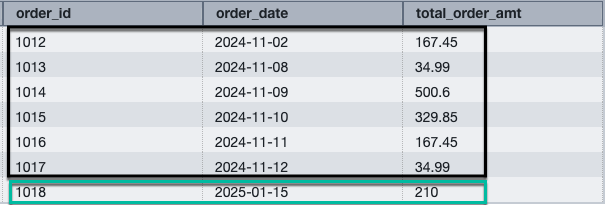
Figure 18: Query results spanning both partition layouts

Converting to a multi-level partition

Iceberg supports multi-level (composite) partition specs, where data is organized by more than one partition field. You can evolve an existing single-level spec into a multi-level spec by adding partition fields one at a time. Each ADD PARTITION FIELD is a lightweight metadata operation, and no data is rewritten.

The orders table is currently partitioned by MONTH(order_date) and bucket(16, customer_id). Add one more partition field to create a three-level spec:

Verify the current partition spec:

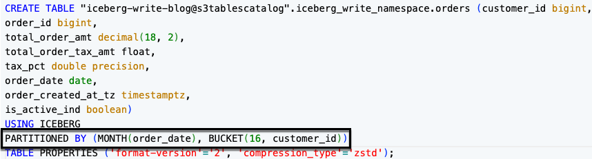
SHOW TABLE "iceberg-write-blog@s3tablescatalog".iceberg_write_namespace.orders;

SHOW TABLE output showing the two-level partition spec of MONTH(order_date) and bucket(16, customer_id)

Figure 19: SHOW TABLE output showing the current two-level partition spec of MONTH(order_date) and bucket(16, customer_id)

Add partition field to build the three-level spec:

-- Add a day-level partition field on order_created_at_tz
ALTER TABLE "iceberg-write-blog@s3tablescatalog".iceberg_write_namespace.orders
ADD PARTITION FIELD day(order_created_at_tz);

Verify the new multi-level partition spec:

SHOW TABLE "iceberg-write-blog@s3tablescatalog".iceberg_write_namespace.orders;

SHOW TABLE output showing the three-level MONTH, bucket, and day partition spec

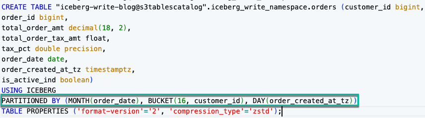
Figure 20: SHOW TABLE output showing the three-level partition spec of MONTH(order_date), bucket(16, customer_id), and day(order_created_at_tz)

After these changes:

Existing data remains in the original single-level layout (month-based folders).
Amazon Redshift writes new data into the multi-level layout (month, then bucket, then day folders).
The query engine reads both layouts transparently.

Dropping partition fields from a multi-level partition

You can also evolve in the other direction by removing partition fields from a multi-level spec to simplify the partition layout. Like adding fields, dropping a partition field is a metadata-only operation and removes one field per statement.

Verify the current multi-level partition spec:

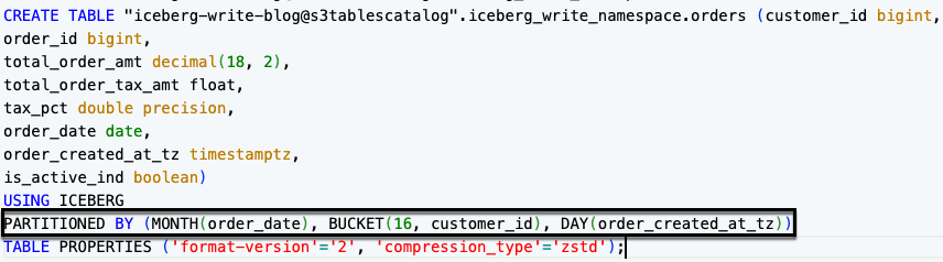
SHOW TABLE "iceberg-write-blog@s3tablescatalog".iceberg_write_namespace.orders;

Figure 21: SHOW TABLE output showing the three-level partition spec before dropping fields

Drop the partition fields one at a time:

-- Drop the bucket partition field
ALTER TABLE "iceberg-write-blog@s3tablescatalog".iceberg_write_namespace.orders
DROP PARTITION FIELD bucket(16, customer_id);
-- Drop the day-level partition field
ALTER TABLE "iceberg-write-blog@s3tablescatalog".iceberg_write_namespace.orders
DROP PARTITION FIELD day(order_created_at_tz);

Verify the table is back to its original single-level spec:

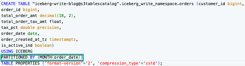
SHOW TABLE "iceberg-write-blog@s3tablescatalog".iceberg_write_namespace.orders;

SHOW TABLE output confirming the table back to a single-level MONTH(order_date) spec

Figure 22: SHOW TABLE output confirming the table is back to a single-level MONTH(order_date) partition spec

After dropping a partition field:

Data written under the dropped field’s layout stays in place and remains queryable.
Amazon Redshift writes new data using only the remaining partition fields.
Queries that filtered on the dropped field still work, but they no longer benefit from partition pruning on that field for newly written data.

Supported partition transforms

The following table lists the partition transforms available for Iceberg tables in Amazon Redshift:

Partition transform	Syntax example	What it does
Year	`year(order_date)`	Groups data into yearly partitions based on a date or timestamp column.
Month	`month(order_date)`	Groups data into monthly partitions based on a date or timestamp column.
Day	`day(order_date)`	Groups data into daily partitions based on a date or timestamp column.
Hour	`hour(event_ts)`	Groups data into hourly partitions based on a timestamp column.
Bucket	`bucket(16, customer_id)`	Distributes data across N hash buckets for even distribution on high-cardinality columns.
Truncate	`truncate(3, zip_code)`	Truncates column values to a fixed width W for grouping similar values together.
Identity	`identity(region)`	Partitions by the exact column value with no transformation applied.

Note: A column that is already part of an existing partition field can’t be used in a new partition field. Drop or replace the existing field first.

Accessing S3 Tables with external schemas

Lake Formation resource links provide cross-engine access to your S3 Tables through centralized governance. You create a resource link in the default AWS Glue Data Catalog that points to your S3 Tables database. Amazon Redshift, Amazon Athena, Amazon EMR, and other engines can then discover and query the tables using a single permission model.

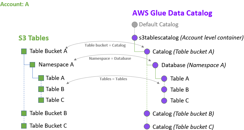
Diagram of S3 Tables integration with AWS Glue Data Catalog and Lake Formation

Figure 23: S3 Tables integration with AWS Glue Data Catalog and Lake Formation

For the complete setup walkthrough, including Lake Formation prerequisites, resource link creation, and permission grants, see Optimize Amazon S3 Tables queries with Amazon Redshift. For conceptual details on resource links and S3 Tables catalog integration, see About resource links and Creating an S3 Tables catalog.

The following steps show how to query S3 Tables through a resource link after completing the setup from the referenced blog.

Grant access to the resource link

In the Lake Formation console, the resource link appears as a database named iceberg_write_blog_rl (type: Resource link). To grant access to the resource link:

In the Lake Formation console, choose Databases.
Locate iceberg_write_blog_rl (type: Resource link).
Choose Actions, then Grant.
Grant DESCRIBE permission to RedshiftIcebergRole.

Create an external schema

With the resource link in place, create an external schema in Amazon Redshift for two-part notation access.

For IAM federated users:

CREATE EXTERNAL SCHEMA s3tables_iceberg
FROM DATA CATALOG
DATABASE 'iceberg_write_blog_rl'
CATALOG_ID '<ACCOUNT_ID>'
IAM_ROLE 'SESSION';

For database users and business intelligence (BI) tools:

CREATE EXTERNAL SCHEMA s3tables_iceberg
FROM DATA CATALOG
DATABASE 'iceberg_write_blog_rl'
IAM_ROLE 'arn:aws:iam::<ACCOUNT>:role/RedshifticebergRole';

Grant access to specific users or roles:

-- Grant to the IAM role used in this walkthrough
GRANT USAGE ON SCHEMA s3tables_iceberg TO "IAMR:RedshifticebergRole";

Amazon Redshift query showing S3 Tables available through the external schema

Figure 24: S3 Tables available through an external schema

Query with two-part notation

With the external schema created, query S3 Tables using two-part notation:

-- Instead of: "iceberg-write-blog@s3tablescatalog".iceberg_write_namespace.orders
SELECT * FROM s3tables_iceberg.orders;

Query results from S3 Tables through the external schema using two-part notation

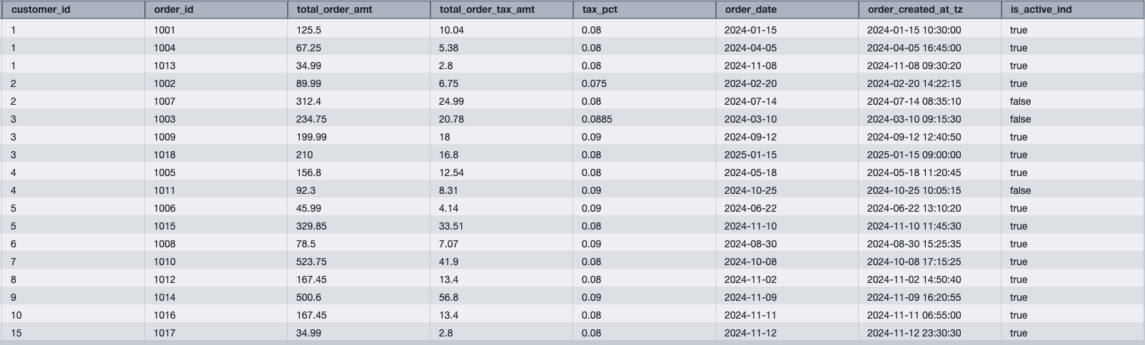
Figure 25: Query results from S3 Tables through an external schema using two-part notation

Access methods comparison

The following table compares the available methods for accessing Iceberg tables in Amazon Redshift:

Access method	Query syntax	Authentication	Best for
S3 Tables three-part notation	`"bucket@s3tablescatalog".namespace.table`	IAM federated identity only	Interactive queries in Query Editor v2 with direct catalog access.
External schema through resource link	`schema_name.table`	Any (IAM role defined in schema)	BI tools, Data API, JDBC/ODBC applications, and shared team access.
awsdatacatalog	`awsdatacatalog.database.table`	IAM federated identity only	Multi-database access in a single session without creating external schemas.

Bringing it together

Combine schema evolution with cross-engine access in a single workflow. The following example adds a column to the orders table and immediately queries it through the external schema:

-- 1. Add a column to the S3 Tables orders table
ALTER TABLE s3tables_iceberg.orders
ADD COLUMN fulfillment_status VARCHAR;
-- 2. Update the new column
UPDATE s3tables_iceberg.orders
SET fulfillment_status = 'shipped'
WHERE order_date < '2024-11-01';
UPDATE s3tables_iceberg.orders
SET fulfillment_status = 'pending'
WHERE order_date >= '2024-11-01';
-- 3. Query immediately via the external schema (no schema recreation needed)
SELECT o.order_id, o.order_date, o.fulfillment_status, c.customer_name
FROM s3tables_iceberg.orders o JOIN demo_iceberg.customer c
ON o.customer_id = c.customer_id
ORDER BY o.order_date DESC;

Query results of a cross-catalog join showing the evolved schema through the external schema

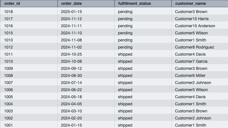
Figure 26: Cross-catalog join showing the evolved schema immediately visible through the external schema

The new column is visible through both the three-part notation and the external schema without any additional configuration, because the schema evolution in Iceberg propagates automatically.

Best practices

Test ALTER operations in non-production first. While metadata-only, schema changes affect all readers immediately.
Use REPLACE PARTITION FIELD instead of DROP + ADD. The atomic operation avoids a transient unpartitioned state.
Monitor partition spec changes with SHOW TABLE. Verify the current spec after any partition evolution.
Choose partition transforms based on query patterns. Use month() or day() for time-range filters. Use bucket() for high-cardinality join keys.
Set table properties before bulk loads. Change compression type (zstd for better ratios, snappy for speed) before large INSERT operations.
Run table maintenance after mutations. After performing multiple UPDATE, DELETE, or MERGE operations, run AWS Glue table optimizers to compact deletion files and improve read performance.
Use Lake Formation for fine-grained access. Column-level and row-level security can be applied through Lake Formation on tables accessed through resource links.
Grant schema access to specific users or roles. Avoid granting to PUBLIC. Use named IAM roles or database users for least-privilege access.
Monitor query performance. Use Amazon Redshift query monitoring features to track performance of write operations and optimize partitioning strategies as needed.

Considerations

Keep the following in mind when working with ALTER TABLE and partition evolution on Iceberg tables:

Plan for metadata-only behavior. ALTER TABLE operations update metadata instantly, and existing data files remain unchanged. All readers see the new schema immediately after the operation completes.
Drop partition fields before dropping partitioned columns. To remove a column used in the current partition spec, first drop or replace the partition field, then drop the column.
Use safe type promotions for ALTER COLUMN TYPE. Amazon Redshift supports widening within compatible families (INT to BIGINT, FLOAT to DOUBLE, DECIMAL(10,2) to DECIMAL(18,2)). Plan column types with future growth in mind.
Account for mixed partition layouts after evolution. Partition evolution doesn’t re-partition existing data. Old files remain in their original layout, and the query engine reads both layouts transparently.
Use external schemas for database user access. The auto-mounted three-part notation ("bucket@s3tablescatalog") requires IAM federated authentication. For database users and BI tools, create an external schema with an explicit IAM role.
Use full three-part notation with awsdatacatalog. The USE statement isn’t supported with awsdatacatalog, so always specify the full path.
Clean up S3 data separately after dropping tables. Dropping an Iceberg table removes only the catalog entry from AWS Glue Data Catalog. Delete the underlying S3 data files separately, or use AWS Glue table optimizers to remove orphaned files.

Clean up

To avoid ongoing charges, run the following:

-- Drop the fulfillment_status column added during testing
ALTER TABLE "iceberg-write-blog@s3tablescatalog".iceberg_write_namespace.orders
DROP COLUMN fulfillment_status;
-- Restore original partition spec (if changed)
ALTER TABLE "iceberg-write-blog@s3tablescatalog".iceberg_write_namespace.orders
REPLACE PARTITION FIELD MONTH(order_date) WITH DAY(order_date);
-- Drop external schema
DROP SCHEMA IF EXISTS s3tables_iceberg;

Conclusion

In this post, you evolved Apache Iceberg table schemas using ALTER TABLE operations. You added, dropped, and renamed columns, widened data types, changed compression, and evolved partition specs, all as metadata-only operations without rewriting data. You also created Lake Formation resource links to provide governed cross-engine access to S3 Tables, and simplified query syntax with external schemas.

This concludes the three-part series on getting started with Apache Iceberg write support in Amazon Redshift:

Part 1: Create Iceberg tables and perform INSERT operations.
Part 2: Run DELETE, UPDATE, and MERGE for row-level modifications.
Part 3: Evolve schemas with ALTER TABLE and add cross-engine access with Lake Formation resource links.

If you have questions or feedback about this series, leave a comment on this post.

Additional resources

Amazon Redshift Iceberg integration – Complete syntax reference.
Writing to Apache Iceberg tables – Detailed examples.
ALTER TABLE for Iceberg – Full ALTER reference.
Amazon S3 Tables – Managed Iceberg storage.
AWS Lake Formation – Centralized data governance.
Optimize S3 Tables queries with Amazon Redshift – Resource links and performance tuning.

About the authors

Enforce IAM permissions boundaries for Amazon SageMaker Unified Studio Tooling blueprints

2026-09-28 Sanjana Sekar

Post Syndicated from Sanjana Sekar original https://aws.amazon.com/blogs/big-data/enforce-iam-permissions-boundaries-for-amazon-sagemaker-unified-studio-tooling-blueprints/

Amazon SageMaker Unified Studio now supports custom permissions boundaries for IAM roles created by the Tooling blueprint. Organizations that enforce Service Control Policies (SCPs) requiring permissions boundaries on all AWS Identity and Access Management (IAM) roles can now adopt Amazon SageMaker Unified Studio without modifying their security posture.

Amazon SageMaker Unified Studio is a unified development environment that brings together data engineering, machine learning, and analytics tools into a single workspace. In Amazon SageMaker Unified Studio, a project is a collaborative workspace that bundles people, tools, and access permissions together. It builds every project from a project profile, which defines a list of blueprints. Blueprints are pre-configured infrastructure templates that provision AWS resources at project creation time or on demand, along with their default parameters. The Tooling blueprint is the only mandatory one. Amazon SageMaker Unified Studio deploys it with every project, creating foundational resources such as the project IAM role and security groups.

In this post, you learn how to create a permissions boundary that restricts AI agent capabilities. You then configure it on the Tooling blueprint using the AWS Command Line Interface (AWS CLI). Finally, you validate that the boundary is enforced on all provisioned roles.

The problem

Enterprises in regulated industries use SCPs to require that every IAM role in an account carries a permissions boundary. A well-scoped boundary prevents privilege escalation and verifies no role exceeds the maximum permissions defined by the organization’s security team. Before this feature, Amazon SageMaker Unified Studio Tooling blueprints created IAM roles without permissions boundaries. When an SCP enforced permissions boundaries, project creation failed with an explicit deny:

User: arn:aws:sts::<account-id>:assumed-role/AmazonSageMakerProvisioning-<account-id>/AmazonDataZoneEnvironmentDeployer-<account-id> is not authorized to perform: iam:CreateRole on resource: arn:aws:iam::<account-id>:role/AmazonBedrockServiceRole-<project-id>-<env-id> with an explicit deny in a service control policy

Amazon SageMaker Unified Studio surfaces the blocked role creation as a Tooling environment provisioning failure, as shown in Figure 1.

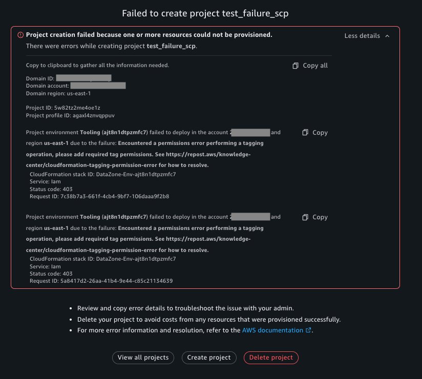
SMUS project overview showing the Tooling environment in a failed state from a permissions boundary SCP denial

Figure 1: Project creation fails when the SCP requires a permissions boundary that is not attached

The project is marked as failed because its Tooling environment couldn’t deploy in the US East (N. Virginia) AWS Region (us-east-1). The details show a 403 permissions error, while the preceding IAM message identifies the underlying iam:CreateRole SCP denial. This blocked adoption for any organization with SCP-enforced permissions boundaries. The AWS CloudFormation event for the Tooling stack exposes the IAM failure behind the project-level error, as shown in Figure 2.

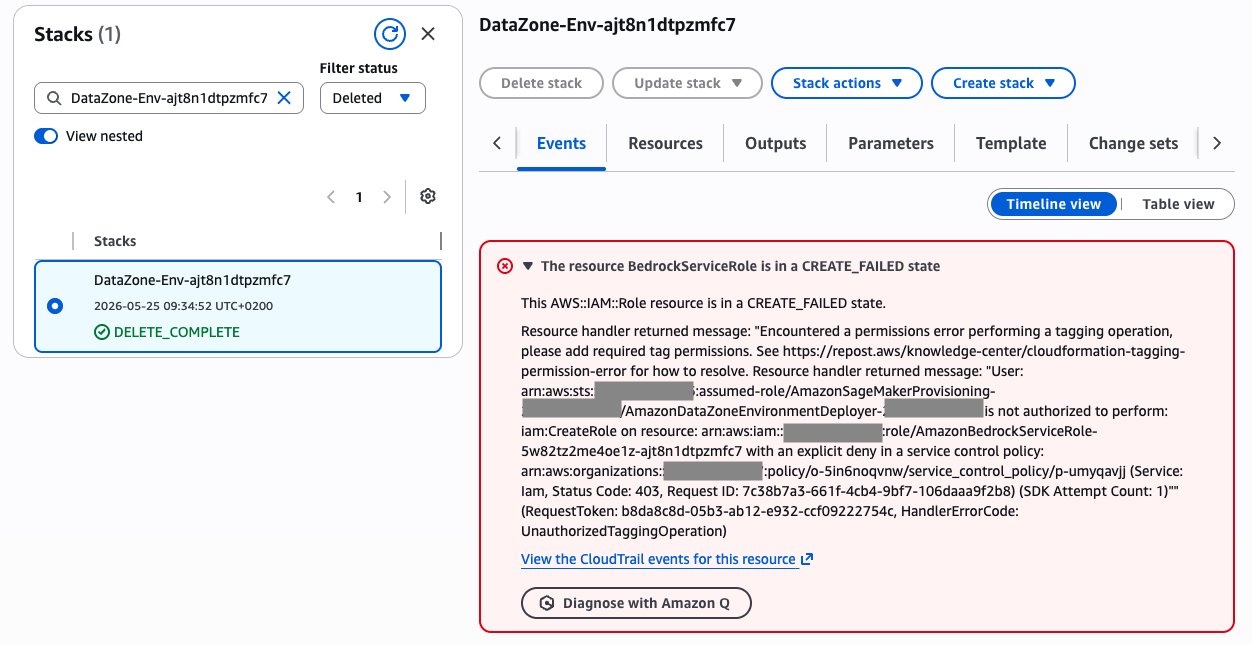
CloudFormation stack events showing the BedrockServiceRole in CREATE_FAILED from an iam:CreateRole SCP explicit deny

Figure 2: Detailed error showing the SCP denial in the Tooling blueprint AWS CloudFormation stack

The AmazonBedrockServiceRole resource entered CREATE_FAILED because iam:CreateRole was explicitly denied by the SCP, even though AWS CloudFormation surfaced the wrapper error as UnauthorizedTaggingOperation.

Granular control using a permissions boundary: Example use case

Beyond satisfying SCP requirements, permissions boundaries give administrators granular control over what the Tooling blueprint roles can do. For instance, some organizations have SecOps policies that require disabling Data Agent and Data Notebook capabilities across their accounts. These organizations want project members to access data connections and run SQL queries directly, but must block conversational AI, code generation, and notebook cell execution through the agent.

When PermissionsBoundaryArn is configured on the Tooling blueprint, SageMaker Unified Studio attaches the specified customer-managed permissions boundary to all IAM roles provisioned by that blueprint. If your governance requires a boundary, configure it explicitly and verify the resulting roles.

The following permissions boundary policy scopes the roles to the AWS services that Amazon SageMaker Unified Studio uses and then explicitly denies the Amazon DataZone actions that power the AI agent. This permissions boundary is provided for illustrative purposes only and isn’t a recommendation or reference for environment configuration. You should tailor your permissions boundaries to your specific workloads in accordance with the principle of least privilege.

{
  "Version": "2012-10-17",
  "Statement": [
    {
      "Sid": "AllowSmusServiceScope",
      "Effect": "Allow",
      "Action": [
        "datazone:*",
        "sagemaker:*",
        "glue:*",
        "s3:*",
        "lakeformation:*",
        "redshift:*",
        "redshift-data:*",
        "redshift-serverless:*",
        "athena:*",
        "q:*",
        "elasticmapreduce:*",
        "bedrock:*",
        "lambda:*",
        "kms:*",
        "secretsmanager:*",
        "codecommit:*",
        "logs:*",
        "cloudwatch:*",
        "sts:AssumeRole",
        "iam:PassRole",
        "ec2:Describe*",
        "ec2:CreateNetworkInterface",
        "ec2:DeleteNetworkInterface",
        "ec2:CreateNetworkInterfacePermission",
        "ec2:DeleteNetworkInterfacePermission"
      ],
      "Resource": "*"
    },
    {
      "Sid": "DenyDataNotebookAndDataAgent",
      "Effect": "Deny",
      "Action": [
        "datazone:*Notebook*",
        "datazone:*Cell*",
        "datazone:*Conversation*",
        "datazone:SendMessage",
        "datazone:GenerateCode",
        "datazone:CancelMessage"
      ],
      "Resource": "*"
    }
  ]
}

Warning: validate before using in production. This example scopes the roles to the service namespaces Amazon SageMaker Unified Studio uses, but it is still coarse (it allows each listed service in full) and is provided only for illustration. Because a permissions boundary is a ceiling, it must remain a superset of everything the three Tooling roles (datazone_usr_role, AmazonBedrockServiceRole, and AmazonBedrockLambdaExecutionRole) actually need. If Amazon SageMaker Unified Studio adds a dependency that isn’t listed, provisioning or in-console actions will fail with an access denied error. Validate in a non-production domain first.

With this boundary attached, the Tooling blueprint provisions normally, project members can access data connections and run SQL queries. However, any attempt to invoke the AI assistant or execute notebook cells through the agent returns an access denied error. The boundary acts as a ceiling that no policy attached to the role can override.

How it works

The custom permissions boundary feature operates at the blueprint configuration level. An administrator sets a PermissionsBoundaryArn in the Tooling blueprint’s regional parameters. When a user creates a new project that includes the Tooling blueprint, Amazon SageMaker Unified Studio provisions an AWS CloudFormation stack that creates three IAM roles and attaches the specified boundary to each:

datazone_usr_role – the role that all project members assume to access data and resources in that project.
AmazonBedrockServiceRole – for Amazon Bedrock operations.
AmazonBedrockLambdaExecutionRole – for Amazon Bedrock-related AWS Lambda functions.

Because the boundary is set at the blueprint level, it applies to every project created under that blueprint. No per-project configuration is needed.

Prerequisites

Before you begin, make sure that you have:

An AWS account with a Amazon SageMaker Unified Studio Identity Center-based domain created.
The Tooling blueprint enabled in the domain.
AWS CLI v2 configured with administrator access.

If your organization uses AWS Organizations with SCPs that require permissions boundaries, you will also need an organization with the target account as a member and permissions to create and attach SCPs in the management account.

Setting up the SCP (optional)

This section provides instructions to create an SCP and attach it to your AWS Organizations organizational unit or accounts. If your organization already enforces permissions boundaries through SCPs, skip this section. Otherwise, create an SCP in your AWS Organizations management account that denies IAM role creation unless an approved permissions boundary is attached. This also prevents the boundary from being removed, swapped, or weakened afterward:

{
  "Version": "2012-10-17",
  "Statement": [
    {
      "Sid": "DenyRoleWithoutApprovedBoundary",
      "Effect": "Deny",
      "Action": [
        "iam:CreateRole",
        "iam:PutRolePermissionsBoundary"
      ],
      "Resource": "*",
      "Condition": {
        "StringNotEquals": {
          "iam:PermissionsBoundary": "arn:aws:iam::${aws:PrincipalAccount}:policy/SMUSToolingBoundary"
        }
      }
    },
    {
      "Sid": "DenyRemovingBoundary",
      "Effect": "Deny",
      "Action": "iam:DeleteRolePermissionsBoundary",
      "Resource": "*"
    },
    {
      "Sid": "ProtectBoundaryPolicy",
      "Effect": "Deny",
      "Action": [
        "iam:DeletePolicy",
        "iam:CreatePolicyVersion",
        "iam:SetDefaultPolicyVersion"
      ],
      "Resource": "arn:aws:iam::${aws:PrincipalAccount}:policy/SMUSToolingBoundary"
    }
  ]
}

This policy does three things:

DenyRoleWithoutApprovedBoundary blocks creating a role, or attaching a boundary to an existing role, with anything other than the approved boundary ARN. Denying iam:PutRolePermissionsBoundary in addition to iam:CreateRole stops a privileged principal from swapping in a weaker boundary after the role exists.
DenyRemovingBoundary blocks iam:DeleteRolePermissionsBoundary outright, so the boundary cannot be stripped off. (This action doesn’t support the iam:PermissionsBoundary condition key, so it must be denied unconditionally.)
ProtectBoundaryPolicy prevents tampering with the boundary policy itself. Deleting it, or publishing and defaulting a new version that quietly widens what it allows.

Note: Scope these denies so you don’t lock yourself out. A broad deny on iam:PutRolePermissionsBoundary and iam:DeleteRolePermissionsBoundary also applies to your own administrators. Add an exception for a break-glass or IAM-admin role (for example, an aws:PrincipalArn StringNotLike condition) so a trusted principal can still manage boundaries.

To create the SCP, sign in to the AWS Organizations console with your management account and go to AWS Organizations → Policies → Service control policies. If SCPs aren’t enabled for your organization yet, choose Enable service control policies first. Choose Create policy, give it a name (for example, test_scp), and replace the default content in the policy editor with the JSON above substituting <account-id> with your account ID. Choose Create policy to save it.

After creating the SCP in the management account, verify its content before attaching it. Figure 3 shows the core create-role control. The full example above adds controls that prevent replacing or removing the boundary and modifying the protected policy.

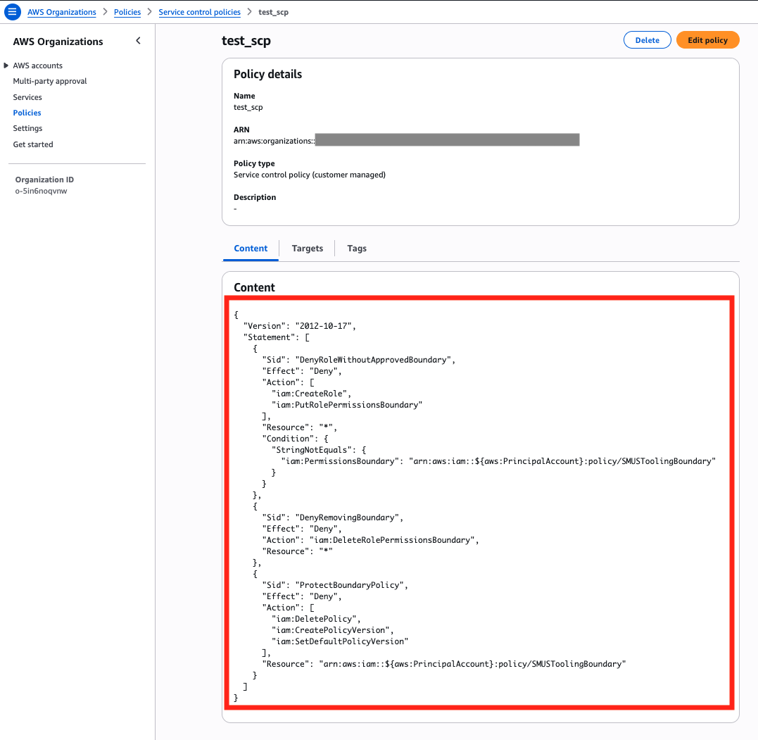
Figure 3: Service Control Policy defined in the AWS Organizations management account

The AWS Organizations Content tab displays the customer-managed test_scp policy. Its visible statement denies iam:CreateRole unless the request uses the SMUSToolingBoundary policy.

Attach this SCP to the organizational unit or account where your Amazon SageMaker Unified Studio domain and domain-associated accounts reside. To do so, open the test_scp service control policy, choose the Targets tab, and choose Attach. The AWS organization structure appears; select the OU or account where the SCP should apply, then choose Attach policy.

Figure 4 identifies the member account that must inherit the SCP in this example organization. The target member account, datazone-account2, resides under OU2, while datazone-account1 is the organization’s management account. Attaching the SCP to the target account or a parent organizational unit enforces it there.

Figure 4: AWS Organizations account structure showing the management account and the target member account

After attaching the policy, verify the association on the SCP’s Targets tab, as shown in Figure 5.

SCP Targets tab listing datazone-account2 as an account target where test_scp is enforced

Figure 5: Service Control Policy attached to the target account where it should be enforced

The Targets tab lists datazone-account2 as an ACCOUNT target, confirming that test_scp is enforced directly on the intended member account.

Configuring the permissions boundary

In this section you will execute the required steps to create the permissions boundary and enable it in the Tooling blueprint. The example in this walkthrough uses us-east-1. Change it to the Region where your Amazon SageMaker Unified Studio domain is deployed. You must execute the configuration in the account where you plan to create your project. This can be your Amazon SageMaker Unified Studio domain account or accounts associated to your Amazon SageMaker Unified Studio domain.

Step 1: Create the permissions boundary policy

If you haven’t already created the boundary policy, save the following JSON document as a boundary-policy.json file on your workstation:

{
    "Version": "2012-10-17",
    "Statement": [
        {
            "Sid": "AllowSmusServiceScope",
            "Effect": "Allow",
            "Action": [
                "datazone:*",
                "sagemaker:*",
                "glue:*",
                "s3:*",
                "lakeformation:*",
                "redshift:*",
                "redshift-data:*",
                "redshift-serverless:*",
                "athena:*",
                "q:*",
                "elasticmapreduce:*",
                "bedrock:*",
                "lambda:*",
                "kms:*",
                "secretsmanager:*",
                "codecommit:*",
                "logs:*",
                "cloudwatch:*",
                "sts:AssumeRole",
                "iam:PassRole",
                "ec2:Describe*",
                "ec2:CreateNetworkInterface",
                "ec2:DeleteNetworkInterface",
                "ec2:CreateNetworkInterfacePermission",
                "ec2:DeleteNetworkInterfacePermission",
                "iam:GetRole",
                "sqlworkbench:*"
            ],
            "Resource": "*"
        },
        {
            "Sid": "DenyDataNotebookAndDataAgent",
            "Effect": "Deny",
            "Action": [
                "datazone:*Notebook*",
                "datazone:*Cell*",
                "datazone:*Conversation*",
                "datazone:SendMessage",
                "datazone:GenerateCode",
                "datazone:CancelMessage"
            ],
            "Resource": "*"
        }
    ]
}

As noted previously, this illustrative policy is scoped to the services Amazon SageMaker Unified Studio uses but is still coarse, and its allow list must stay a superset of what all three Tooling roles need.

Then create the policy using the following command:

aws iam create-policy \
--policy-name SMUSToolingBoundary \
--policy-document file://boundary-policy.json \
--description "Permissions boundary for SMUS Tooling roles - denies Data Agent and Data Notebook capabilities"

Note the policy ARN from the output, because it will be used later in the procedure.

Step 2: Retrieve the ID of your domain

Retrieve the ID of your domain by running the following command. Replace <YOUR_DOMAIN_NAME> with the name of your SageMaker Unified Studio domain.

aws datazone list-domains \
--region us-east-1 \
--query "items[?name=='<YOUR_DOMAIN_NAME>'].id | [0]" \
--output text

Note the returned ID, because it will be used later in the procedure.

Step 3: Identify the Tooling blueprint

Retrieve the Tooling blueprint ID by running the following command. Replace <domain-id> with the ID you noted in Step 2.

aws datazone list-environment-blueprints \
  --domain-identifier <domain-id> \
  --managed \
  --region eu-west-1 \
  --query "items[?name=='Tooling'].id" \
  --output json | jq -r '.[0]'

Note the returned ID, because it will be used later in the procedure.

Step 4: Read the current configuration

Retrieve the current Tooling blueprint configuration by executing the following command. Replace <domain-id> with the ID from Step 2 and <tooling-bp-id> with the ID from Step 3.

aws datazone get-environment-blueprint-configuration \
--domain-identifier <domain-id> \
--environment-blueprint-identifier <tooling-bp-id> \
--region us-east-1 | tee tooling-bp-config-backup.json

Important: Back up the output of get-environment-blueprint-configuration before making any changes. The command above pipes the response to tooling-bp-config-backup.json so you have a restore point if you need to revert.

Note the values of provisioningRoleArn, manageAccessRoleArn, enabledRegions, and all fields inside regionalParameters (AZs, S3Location, Subnets, VpcId). You will need all of these in the next step.

Step 5: Set the permissions boundary

Update the blueprint configuration to include PermissionsBoundaryArn in the regional parameters using the following command.

Important: The put-environment-blueprint-configuration API operates in overwrite mode, it replaces the entire configuration with what you provide. You must include all existing values from the previous step’s output. The only new addition is PermissionsBoundaryArn inside the regional parameters. Omitting any existing parameter removes it.

Make sure to replace <domain-id> with the ID you noted in Step 2, <tooling-bp-id> with the ID you noted in Step 3, and all other <placeholder> values with the corresponding values from Step 4’s output.

aws datazone put-environment-blueprint-configuration \
--domain-identifier <domain-id> \
--environment-blueprint-identifier <tooling-bp-id> \
--enabled-regions '<enabledRegions>' \
--provisioning-role-arn "<provisioningRoleArn>" \
--manage-access-role-arn "<manageAccessRoleArn>" \
--regional-parameters '{
  "<region>": {
    "AZs": "<AZs>",
    "S3Location": "<S3Location>",
    "Subnets": "<Subnets>",
    "VpcId": "<VpcId>",
    "PermissionsBoundaryArn": "arn:aws:iam::<account-id>:policy/SMUSToolingBoundary"
  }
}' \
--region <region>

The following anonymized example is based on an existing Tooling blueprint configuration. Its S3Location reflects the bucket naming pattern used in that environment. Copy the exact S3Location returned in Step 4. Don’t use the following illustrative value. Here’s an example:

aws datazone put-environment-blueprint-configuration \
--domain-identifier <domain-id> \
--environment-blueprint-identifier <tooling-bp-id> \
--enabled-regions '["us-east-1"]' \
--provisioning-role-arn "arn:aws:iam::<account-id>:role/service-role/AmazonSageMakerProvisioning-<account-id>" \
--manage-access-role-arn "arn:aws:iam::<account-id>:role/service-role/AmazonSageMakerManageAccess-us-east-1-<domain-id>" \
--regional-parameters '{
  "us-east-1": {
    "AZs": "us-east-1a,us-east-1b,us-east-1c,us-east-1d",
    "S3Location": "s3://amazon-sagemaker-<account-id>-us-east-1-<suffix>",
    "Subnets": "<subnet-1>,<subnet-2>,<subnet-3>,<subnet-4>",
    "VpcId": "<vpc-id>",
    "PermissionsBoundaryArn": "arn:aws:iam::<account-id>:policy/SMUSToolingBoundary"
  }
}' \
--region us-east-1

Step 6: Verify the configuration was applied

Confirm the permissions boundary ARN is now set in the blueprint configuration using the following command. Make sure to replace <domain-id> with the ID you noted in Step 2 and <tooling-bp-id> with the ID you noted in Step 3.

aws datazone get-environment-blueprint-configuration \
--domain-identifier <domain-id> \
--environment-blueprint-identifier <tooling-bp-id> \
--region us-east-1 \
--query "regionalParameters.\"us-east-1\".PermissionsBoundaryArn"

The output should return your boundary policy ARN:

"arn:aws:iam::<account-id>:policy/SMUSToolingBoundary"

Validating the configuration

After configuring the permissions boundary, in this section you will get instructions to create a new project to verify it works end to end and that the IAM roles created with the project actually include the permissions boundary.

Step 1: Select a project profile in enabled state

Use the following command to list project profiles configured in your domain. Make sure to replace <domain-id> with the ID you noted in Step 2 of the “Configuring the permissions boundary” section.

aws datazone list-project-profiles \
--domain-identifier <domain-id> \
--region us-east-1

Choose a project profile that has "status": "ENABLED". Note the id of any project profile returned in the previous command.

Step 2: Create a test project

Create a new project using the following command. Make sure to replace <domain-id> with the ID you noted in Step 2 of the “Configuring the permissions boundary” section and to replace <profile-id> with the project profile ID noted in Step 1 of this section.

aws datazone create-project \
--domain-identifier <domain-id> \
--name "PB-Validation-$(date +%Y%m%d-%H%M%S)" \
--project-profile-id <profile-id> \
--region us-east-1

Note the id (project ID) returned in the response. Wait for the Tooling blueprint to provision. This typically takes a minute or two. After provisioning completes, confirm that the validation project reaches the Active state, as shown in Figure 6.

SMUS Projects list showing the timestamped PB-Validation project in Active status after successful creation

Figure 6: Project created successfully with the permissions boundary configured

The Projects list shows the timestamped PB-Validation-* project with an Active status, confirming that project creation succeeded with the custom boundary configured.

Step 3: Verify the roles have the boundary attached

In this section you check that the IAM roles created with the project have the permissions boundary attached. Use the following commands to get the configuration for the IAM roles created with the project you just created. Replace <domain-id> and <project-id> with the values from the previous steps.

# Get the environment ID
ENV_ID=$(aws datazone list-environments \
--domain-identifier <domain-id> \
--project-identifier <project-id> \
--region us-east-1 \
--query "items[?name=='Tooling'].id" --output text)

# List IAM roles in the AWS CloudFormation stack
aws cloudformation describe-stack-resources \
--stack-name "DataZone-Env-${ENV_ID}" \
--region us-east-1 \
--query "StackResources[?ResourceType=='AWS::IAM::Role'].PhysicalResourceId" \
--output table

# Verify each role has the boundary
aws iam get-role \
--role-name "<role-name>" \
--query 'Role.PermissionsBoundary'

All three roles should return a response showing the permissions boundary ARN:

{
  "PermissionsBoundaryType": "Policy",
  "PermissionsBoundaryArn": "arn:aws:iam::<account-id>:policy/SMUSToolingBoundary"
}

You can also verify each role in the IAM console. Figure 7 shows the permissions boundary for the project user role.

IAM console Permissions tab showing SMUSToolingBoundary as the permissions boundary on datazone_usr_role

Figure 7: IAM console showing the permissions boundary attached to the datazone_usr_role

The datazone_usr_role Permissions tab displays SMUSToolingBoundary as its customer-managed permissions boundary.

Figure 8 confirms that the same boundary is attached to the Amazon Bedrock service role.

IAM console showing SMUSToolingBoundary as the permissions boundary on AmazonBedrockServiceRole

Figure 8: IAM console showing the permissions boundary attached to the AmazonBedrockServiceRole

The AmazonBedrockServiceRole also displays SMUSToolingBoundary as its customer-managed permissions boundary.

Figure 9 verifies the boundary on the third Tooling role, the Bedrock Lambda execution role.

IAM console showing SMUSToolingBoundary as the permissions boundary on AmazonBedrockLambdaExecutionRole

Figure 9: IAM console showing the permissions boundary attached to the AmazonBedrockLambdaExecutionRole

The AmazonBedrockLambdaExecutionRole likewise displays SMUSToolingBoundary, confirming that all three provisioned roles carry the boundary.

Step 4: Verify the boundary denies AI agent actions

In this section you verify the boundary actually denies AI agent actions. If you configured the boundary from the use case section earlier, the boundary blocks Data Notebooks and messages to the Data Agent, such as the Query Editor assistant. Any such attempt returns an access denied error. The project user role has the boundary attached, so even if the role’s identity policies grant the relevant APIs, the boundary’s explicit deny takes precedence.

To confirm, navigate to your project in SageMaker Unified Studio and test the following actions:

Attempt to create a notebook – In the left sidebar, select Notebooks. Select Create notebook. The operation will fail because the permissions boundary prevents the datazone:CreateNotebook action (Figure 10).

Figure 10: Permissions boundary preventing creation of Data Notebooks

After the create action, Amazon SageMaker Unified Studio reports Failed to create notebook and identifies datazone:CreateNotebook as explicitly denied by SMUSToolingBoundary.

Attempt to use Data Agent in the Query Editor – In the left sidebar, select Query Editor, then select the Chat with AI icon. The agent chat will fail to load because the permissions boundary blocks the APIs required by Data Agent (Figure 11).

Figure 11: Permissions boundary preventing using Data Agent on Query Editor

The Query Editor remains available, but the Agent panel reports “You don’t have access to Data Agent“. In this configured test, that message is the user-visible result of denying the Data Agent APIs. The screenshot itself doesn’t display the denied API or boundary ARN.

Important considerations

Immutable after project creation – The permissions boundary is set at provisioning time. Changing the boundary ARN on the blueprint configuration only affects new projects. Existing projects retain their original boundary.
Applies to all Tooling-provisioned roles – When PermissionsBoundaryArn is configured on the Tooling blueprint, SageMaker Unified Studio attaches the specified customer-managed permissions boundary to all three IAM roles created by that blueprint. It’s applied uniformly — you can’t selectively apply it to individual roles. No boundary is attached unless you configure one, so if your governance requires a boundary, set it explicitly and verify the resulting roles rather than assuming one is present by default.
Policy must exist – The IAM policy referenced by PermissionsBoundaryArn must exist in the account before project creation. If the policy is deleted or the ARN is invalid, provisioning will fail.
Tooling blueprint only – Among Amazon SageMaker Unified Studio provided blueprints, only the Tooling blueprint supports custom permissions boundaries. Other provided blueprints that create IAM roles (for example, the EmrOnEc2 blueprint) don’t currently support this feature. If your organization requires permissions boundaries on roles created by additional blueprints, you can build custom blueprints that include a permissions boundary configuration so you can extend this security control across your entire project infrastructure.

Clean up

To remove test resources, delete the test project from the SageMaker Unified Studio UI. On the project’s Overview page, choose the ⋮ (more actions) menu in the top-right and choose Delete project.

Figure 12: Deleting the test project from the project Overview page.

In the Delete project dialog, type confirm in the text box to acknowledge that the action is final, then choose Delete project. This permanently deletes the project and its underlying resources, and triggers an asynchronous AWS CloudFormation stack deletion.

Figure 13: Confirming project deletion.

To remove the boundary from future projects, re-run the put-environment-blueprint-configuration command from Step 5: Set the permissions boundary, but omit the PermissionsBoundaryArn field from the regional parameters. Because you backed up the original configuration in Step 4: Read the current configuration (tooling-bp-config-backup.json), you can reuse the exact same provisioningRoleArn, manageAccessRoleArn, enabledRegions, and regionalParameters values (AZs, S3Location, Subnets, VpcId) — just without PermissionsBoundaryArn — so the blueprint returns to provisioning roles with no permissions boundary.

Conclusion

With the custom permissions boundary feature for Amazon SageMaker Unified Studio, organizations can adopt Amazon SageMaker Unified Studio Tooling blueprints without compromising their IAM governance posture. By configuring a single parameter on the Tooling blueprint, all IAM roles provisioned by future projects automatically carry the specified permissions boundary. This satisfies SCPs that mandate a boundary on every role and gives administrators granular control over what the Tooling roles can do, for example disabling AI agent and notebook capabilities. Remember that the example boundary in this post is illustrative, because it scopes to the services SageMaker Unified Studio uses but is still coarse.

“I just updated the EnvironmentBlueprintConfiguration for the Tooling blueprint to include the new PermissionsBoundaryArn param. After that the blueprint provisioned successfully with the required permissions boundary attached to all the IAM roles, in line with our security policies. In the end it was a one-line change.”

— Nat Noordanus, Data Tech Lead at Nexthink

To get started, create your permissions boundary policy, configure it on the Tooling blueprint using the CLI, and create a project to verify the boundary is attached.

For more information, see the documentation for Amazon SageMaker Unified Studio, IAM permissions boundaries, and Service Control Policies.

About the authors

[$] Reducing undefined behavior in the C language

2026-09-28 corbet

Post Syndicated from corbet original https://lwn.net/Articles/1095811/

As a professor of biomedical engineering, Martin Uecker perhaps does not
fit the profile of a typical presenter at Kernel Recipes. He is,
however, a longtime Linux user, and works on free software for controlling
magnetic resonance imaging (MRI) scanners. He was at the conference to
talk about the C programming language, the specific problem of undefined
behavior in C, and whether it can eventually be made into a memory-safe
language.

Comic for 2026.09.28 – Abled

2026-09-28 Explosm.net

Post Syndicated from Explosm.net original https://explosm.net/comics/abled

New Cyanide and Happiness Comic

Security updates for Monday

2026-09-28 jake

Post Syndicated from jake original https://lwn.net/Articles/1097191/

Security updates have been issued by AlmaLinux (firefox, ipa, kernel, libxml2, perl-DBI, python-cryptography, thunderbird, and unbound), Debian (chromium, evolution-data-server, exim4, ghostscript, incus, lemonldap-ng, libheif, nodejs, php8.4, ruby-oj, swift, and vlc), Fedora (chromium, cinnamon, cinnamon-desktop, cinnamon-session, cinnamon-settings-daemon, ckermit, dnf5, forgejo, goose, gssntlmssp, libheif, libpcap, librsvg2, mingw-gstreamer1, mingw-gstreamer1-plugins-bad-free, mingw-gstreamer1-plugins-base, mingw-gstreamer1-plugins-good, mingw-python3, mongo-c-driver, muffin, nemo, nemo-extensions, nextcloud, pgadmin4, postgresql16-postgis, postgresql17-postgis, postgresql18-postgis, rust-librsvg, rust-xml5ever, sipp, suricata, tesseract, and xreader), Mageia (erlang, gpsd, libreswan, python3 & python-pip, and udisks2), Oracle (abrt, buildah, cockpit-image-builder, corosync, ipa, kernel, libxml2, openexr, perl-DBI, perl-DBI:1.641, postgresql, thunderbird, unbound, and yelp), SUSE (389-ds, ansible-lint, cups, firefox, flatpak-builder, forgejo-longterm, gdb, gimp, gitoxide, glib2, gnome-shell, google-guest-agent, google-osconfig-agent, haveged, helm, ImageMagick, kbd, libsoup, libtpms, obs-service-cargo, openai-codex, opensuse-signkey-cert, osmo-iuh, perl-mojolicious, poppler, python-WebOb, python-WebOb-doc, python313-vllm, python314, sdbootutil, suseconnect-ng, and swtpm), and Ubuntu (exim4, freerdp3, libvirt, libvirt-hwe, libwebsockets, lxc, pyjwt, and requests).

Next.js applications, powered by Vite: introducing Vinext 1.0

2026-09-28 James Anderson

Post Syndicated from James Anderson original https://blog.cloudflare.com/vinext-nextjs-on-vite/

When we launched Vinext in February, it was the result of an audacious week-long AI-driven experiment to see how far one engineer, and a stack of tokens, could get to replicating the NextJS framework backed by Vite.

In the seven months since that experiment, Vinext has grown into a framework that our customers trust and run in production for high-traffic, dynamic applications.

Today we are announcing the release of Vinext 1.0, the latest step on our journey to make it possible to deploy Next.js apps anywhere. Vinext lets you take any Next.js application, whether it was built for the Pages or App Router, and make it portable to be deployed to any web platform, including the Cloudflare Workers free plan, Netlify, or AWS Lambda.

Vinext 1.0 brings with it sweeping improvements to compatibility, stability, and caching behaviors, and sets the project up for the long term. There’s never been a better time to take your Next.js project and convert it to Vinext; just run npx vinext check and npx vinext init.

Graduation to 1.0

On release Vinext was promising, but it was incomplete. Since then, we’ve spent a lot of time both improving App Router compatibility and expanding that to Pages Router apps — which we’ve learned many customers are longtime fans of, with large applications that are complex to migrate. We didn’t want Vinext to be a tool that only worked for people using the latest App Router features.

Our focus has been on adopting both these routers, and watching our test compatibility closely, which for most important customer-requested features now surpasses 99%.

This improvement has been fueled through the community around our GitHub project. As soon as Vinext launched, that community threw it at a wide variety of applications to find the gaps. With their scrutiny, we found challenges not immediately obvious in the test coverage. Vinext needs to act exactly as Next.js behaves. It is not good enough to imitate functions with the same name. Building an alternative import { revalidatePath } is simple enough; the difficulty is in making sure it correctly affects the rendered pages, cache entry, and future requests.

Tracing requests through the application to make sure Vinext responds in the way expected — and replicating not just the API, but the behavior of this machine — was by far the more challenging aspect.

Once we’ve patched problems and brought new features forward, it’s important that we don’t regress, especially if Next.js makes a change. That’s why we’ve also built out our test suite: thousands of focused tests covering core framework behavior across both routers, the development and production server, and the deployment targets of Nodejs and Cloudflare Workers. We also run the Next.js end-to-end test suite against Vinext nightly, giving us a continually moving window on our compatibility, and making sure we immediately become aware of regressions coming from merged changes. Alongside the automated testing, we’ve been working directly with large customers that have Vinext in production to make sure they are not facing issues.

What’s in 1.0

The clearest messages we got from customers using Vinext is that certain Next.js features carry the framework and Vinext didn’t actually need to do everything that Next.js has launched in recent versions to be incredibly useful to them. So we focused on better support where you need it:

App Router, Pages Router, and Hybrid applications: We heard from customers that Pages Router was still important, and migrations are not a one-step process. Vinext therefore has support for both routing paths, including React Server Components, Server Actions, API routes, route handlers, middleware, and client-side navigation.
The complete page lifecycle: Pages can be rendered in many different ways: on the server, pre-rendered in the build, exported as static assets, or cached with page-level Incremental Static Regeneration (ISR). We’ve made sure that Background and on-demand revalidation work with any output.
Caching: Vinext has a shared set of caching functions across the App and Pages Router and the supported runtimes. We have further support for using Cloudflare’s Workers Cache.
Observability: Vinext provides Next.js-compatible tracing across both routers, so existing OpenTelemetry and Sentry setups continue to work. On Cloudflare Workers, traces also integrate with native Workers Observability.
Next.js ecosystem compatibility: Vinext implements the public next/* surface and supports common Next patterns for use of authentication, MDX, image optimization, fonts, metadata, environment variables, and more.
First-class runtime support for Workers: While Vinext can run anywhere, server code can run in the Cloudflare workerd runtime during development and production, with direct access to bindings such as image optimization and hyperdrive.

We’ve also made migration part of the framework: it takes two commands to verify that your Next.js install and any modification you have made is compatible, and set up the Vite and deployment configuration while keeping all your previous Next.js project structure.

When we talked to teams about what features were important for them, something stood out. Next.js 16 took a stance that Cache Components were an important part of the future of the framework, and yet most teams that we talked to were not using them and did not consider support a prerequisite to move. Therefore, Vinext today has limited support for the “use cache” directive that drives Cache Components, and though we will continue to improve compatibility there, we’re much more focused on the core priorities above.

Pre-rendering and cache warming

When we first announced Vinext, it supported Incremental Static Regeneration (ISR) after the first request, but it did not yet render pages during the build. Applications use generateStaticParams() and getStaticPaths() to identify pages that should be rendered when building, and they expect page-level ISR to connect those initial responses to background and on-demand revalidation.

Vinext 1.0 supports that lifecycle for both routers. It can prerender App Router and Pages Router routes during the build, serve those responses through page-level ISR, and invalidate them by path or tag. It also supports output: "export" when the result you want is a fully static site.

But this led us to question something: Why should this rendering happen during the build at all?

A site with tens or hundreds of thousands of possible URLs can spend a seriously long time rendering pages that receive little traffic. The build process cannot evaluate the long tail of traffic that most sites experience and therefore cannot focus compute time on the smaller number of more critical pages. Instead you waste hours of time waiting for sequential builds working their way through thousands of pages, long after the most important routes are done.

Cache warming is our solution to this, moving page prerendering from the build machine to Cloudflare’s network. Developers can continue to use Next.js primitives to identify the pages for prerendering, and Vinext can additionally identify high-traffic pages to add to this list. This happens in the background before your site is deployed to production, so that the moment it is, it is ready to serve rapid responses from the Cloudflare cache.

Inside the deployment process, this works by uploading a new Worker version and deploying it to 0% of production traffic, before then requesting pages specifically from that version. This allows the rendering pipeline to work before any real users hit the new deployment. Once the caches have been populated, the deployment can be promoted safely.

What we’re doing next

If the original experiment invented the one-off slopfork, the more consequential part has been how we can keep that process of self-improvement running indefinitely.

The project is now focused on keeping the framework up to date with everything happening upstream. Next.js canary receives new commits every day. Each morning, an agent reviews the changes, fetches diffs, and opens tracking issues for anything that could affect Vinext. Every night, the compatibility matrix is regenerated as we run the Next.js test suite against Vinext.

When one of these tests or issues reveals a gap, agents are now in the position where they can identify the change across both codebases, build a reproduction, port any relevant tests, and propose a fix.

This review has been catching missing cases, unsafe caching behaviors, and differences in the development vs. production servers.

Automation has helped us narrow the stream of activity into a focused set of changes that deserve attention, allowing the maintainers of the project to focus on only the issues that need context of how a process should map onto Vite from the Next.js implementation.

We’re building a software factory for open source at Cloudflare, and you can see what we’re up to on GitHub.

Try it out

Vinext is available for new applications, and existing Next.js projects.

Start a new application today:

Or migrate an existing application:

And then deploy it to Cloudflare Workers, with our cache warming:

Visit vinext.dev for documentation, examples, and the current compatibility matrix. Vinext is open source at github.com/cloudflare/vinext. Issues, pull requests, application reproductions, and feedback are welcome.

One bus, shared with the organization

Publishing in the format teams already use

Self-service onboarding for application teams

History for consumers that did not exist yet

Order, where order matters

Reshaping events, and delivering directly to a target

Conclusion

Latency-sensitive data processing

Why Lambda fits latency-sensitive data processing

New network throughput behavior for Lambda functions

Solution overview

Prerequisites

Mode 1: Processing pre-partitioned data

Mode 2: Processing single large objects

Results

Clean up

Best practices

Profiling and planning

Implementation

Conclusion

The business problem

Solution architecture

A real incident

Remediation

How it works

Results

Getting started

Clean up

Conclusion

Related resources

About the authors

An independent cloud for Europe

Built to meet regulatory standards

Standalone and fully secure

Customer data stays in the EU

Learn more

Why auditing an autonomous agent is different

The four surfaces

The agent journal

Recommendations polling

Amazon EventBridge lifecycle events

AWS CloudTrail

IAM: Action boundary

The reference architecture

Querying the archive: AWS Glue and Athena

Access control

Closing the loop: Correlating findings to actual changes

Correlating agent actions

Production considerations

The full loop

Operating the pipeline: Common failures

Limitations

Conclusion

About the authors

How SES tenant isolation works

How Mail Manager works

Understanding the outbound email flow

Compare the patterns

Pattern 1: The SMTP sender sets the header before Mail Manager

Pattern 2: Mail Manager adds a static header with Add header

Pattern 3: Mail Manager derives the header from rule conditions

Scale limits of Pattern 3

Pattern 4: Mail Manager calls Lambda for runtime tenant resolution

Pattern 5: Mail Manager stages to Amazon S3, Lambda delivers asynchronously

Secure tenant attribution with IAM

Paused tenants

Observability

Limits that shape the architecture

Conclusion

Next steps

About the authors

Solution overview

Prerequisites

Schema evolution with ALTER TABLE

Add a column

Drop a column

Rename a column

Widen a column type

Set table properties

Partition evolution