When you’re dealing with large amounts of data, it’s helpful to get a quick overview — which is exactly what aggregations provide in SQL. Aggregations, known as “GROUP BY queries”, provide a bird’s eye view, so you can quickly gain insights from vast volumes of data.
That’s why we are excited to announce support for aggregations in R2 SQL, Cloudflare’s serverless, distributed, analytics query engine, which is capable of running SQL queries over data stored in R2 Data Catalog. Aggregations will allow users of R2 SQL to spot important trends and changes in the data, generate reports and find anomalies in logs.
This release builds on the already supported filter queries, which are foundational for analytical workloads, and allow users to find needles in haystacks of Apache Parquet files.
In this post, we’ll unpack the utility and quirks of aggregations, and then dive into how we extended R2 SQL to support running such queries over vast amounts of data stored in R2 Data Catalog.
The importance of aggregations in analytics
Aggregations, or “GROUP BY queries”, generate a short summary of the underlying data.
A common use case for aggregations is generating reports. Consider a table called “sales”, which contains historical data of all sales across various countries and departments of some organisation. One could easily generate a report on the volume of sales by department using this aggregation query:
SELECT department, sum(value)
FROM sales
GROUP BY department
The “GROUP BY” statement allows us to split table rows into buckets. Each bucket has a label corresponding to a particular department. Once the buckets are full, we can then calculate “sum(value)” for all rows in each bucket, giving us the total volume of sales performed by the corresponding department.
For some reports, we might only be interested in departments that had the largest volume. That’s where an “ORDER BY” statement comes in handy:
SELECT department, sum(value)
FROM sales
GROUP BY department
ORDER BY sum(value) DESC
LIMIT 10
Here we instruct the query engine to sort all department buckets by their total sales volume in the descending order and only return the top 10 largest.
Finally, we might be interested in filtering out anomalies. For example, we might want to only include departments that had more than five sales total in our report. We can easily do that with a “HAVING” statement:
SELECT department, sum(value), count(*)
FROM sales
GROUP BY department
HAVING count(*) > 5
ORDER BY sum(value) DESC
LIMIT 10
Here we added a new aggregate function to our query — “count(*)” — which calculates how many rows ended up in each bucket. This directly corresponds to the number of sales in each department, so we have also added a predicate in the “HAVING” statement to make sure that we only leave buckets with more than five rows in them.
Two approaches to aggregation: compute sooner or later
Aggregation queries have a curious property: they can reference columns that are not stored anywhere. Consider “sum(value)”: this column is computed by the query engine on the fly, unlike the “department” column, which is fetched from Parquet files stored on R2. This subtle difference means that any query that references aggregates like “sum”, “count” and others needs to be split into two phases.
The first phase is computing new columns. If we are to sort the data by “count(*)” column using “ORDER BY” statement or filter rows based on it using “HAVING” statement, we need to know the values of this column. Once the values of columns like “count(*)” are known, we can proceed with the rest of the query execution.
Note that if the query does not reference aggregate functions in “HAVING” or “ORDER BY”, but still uses them in “SELECT”, we can make use of a trick. Since we do not need the values of aggregate functions until the very end, we can compute them partially and merge results just before we are about to return them to the user.
The key difference between the two approaches is when we compute aggregate functions: in advance, to perform some additional computations on them later; or on the fly, to iteratively build results the user needs.
First, we will dive into building results on the fly — a technique we call “scatter-gather aggregations.” We will then build on top of that to introduce “shuffling aggregations” capable of running extra computations like “HAVING” and “ORDER BY” on top of aggregate functions.
Scatter-gather aggregations
Aggregate queries without “HAVING” and “ORDER BY” can be executed in a fashion similar to filter queries. For filter queries, R2 SQL picks one node to be the coordinator in query execution. This node analyzes the query and consults R2 Data Catalog to figure out which Parquet row groups may contain data relevant to the query. Each Parquet row group represents a relatively small piece of work that a single compute node can handle. Coordinator node distributes the work across many worker nodes and collects results to return them to the user.
In order to execute aggregate queries, we follow all the same steps and distribute small pieces of work between worker nodes. However, this time instead of just filtering rows based on the predicate in the “WHERE” statement, worker nodes also compute pre-aggregates.
Pre-aggregates represent an intermediary state of an aggregation. This is an incomplete piece of data representing a partially computed aggregate function on a subset of data. Multiple pre-aggregates can be merged together to compute the final value of an aggregate function. Splitting aggregate functions into pre-aggregates allows us to horizontally scale computation of aggregation, making use of vast compute resources available in Cloudflare’s network.
For example, pre-aggregate for “count(*)” is simply a number representing the count of rows in a subset of data. Computing the final “count(*)” is as easy as adding these numbers together. Pre-aggregate for “avg(value)” consists of two numbers: “sum(value)” and “count(*)”. The value of “avg(value)” can then be computed by adding together all “sum(value)” values, adding together all “count(*)” values and finally dividing one number by the other.
Once worker nodes have finished computing the pre-aggregates, they stream results to the coordinator node. The coordinator node collects all results, computes final values of aggregate functions from pre-aggregates, and returns the result to the user.
Shuffling, beyond the limits of scatter-gather
Scatter-gather is highly efficient when the coordinator can compute the final result by merging small, partial states from workers. If you run a query like SELECT sum(sales) FROM orders, the coordinator receives a single number from each worker and adds them up. The memory footprint on the coordinator is negligible regardless of how much data resides in R2.
However, this approach becomes inefficient when the query requires sorting or filtering based on the result of an aggregation. Consider this query, which finds the top two departments by sales volume:
SELECT department, sum(sales)
FROM sales
GROUP BY department
ORDER BY sum(sales) DESC
LIMIT 2
Correctly determining the global Top 2 requires knowing the total sales for every department across the entire dataset. Because the data is spread effectively at random across the underlying Parquet files, sales for a specific department are likely split across many different workers. A department might have low sales on every individual worker, excluding it from any local Top 2 list, yet have the highest sales volume globally when summed together.
The diagram below illustrates how a scatter-gather approach would not work for this query. “Dept A” is the global sales leader, but because its sales are evenly spread across workers, it doesn’t make to some local Top 2 lists, and ends up being discarded by the coordinator.
Consequently, when the query orders results by their global aggregation, the coordinator cannot rely on pre-filtered results from workers. It must request the total count for every department from every worker to calculate the global totals before it can sort them. If you are grouping by a high-cardinality column like IP addresses or User IDs, this forces the coordinator to ingest and merge millions of rows, creating a resource bottleneck on a single node.
To solve this, we need shuffling, a way to colocate data for specific groups before the final aggregation occurs.
Shuffling of aggregation data
To address the challenges of random data distribution, we introduce a shuffling stage. Instead of sending results to the coordinator, workers exchange data directly with each other to colocate rows based on their grouping key.
This routing relies on deterministic hash partitioning. When a worker processes a row, it hashes the GROUP BY column to identify the destination worker. Because this hash is deterministic, every worker in the cluster independently agrees on where to send specific data. If “Engineering” hashes to Worker 5, every worker knows to route “Engineering” rows to Worker 5. No central registry is required.
The diagram below illustrates this flow. Notice how “Dept A” starts on Workers 1, 2 and 3. Because the hash function maps “Dept A” to Worker 1, all workers route those rows to that same destination.
Shuffling aggregates produces the correct results. However, this all-to-all exchange creates a timing dependency. If Worker 1 begins calculating the final total for “Dept A” before Worker 3 has finished sending its share of the data, the result will be incomplete.
To address this, we enforce a strict synchronization barrier. The coordinator tracks the progress of the entire cluster while workers buffer their outgoing data and flush it via gRPC streams to their peers. Only when every worker confirms that it has finished processing its input files and flushing its shuffle buffers does the coordinator issue the command to proceed. This barrier guarantees that when the next stage begins, the dataset on each worker is complete and accurate.
Local finalization
Once the synchronization barrier is lifted, every worker holds the complete dataset for its assigned groups. Worker 1 now has 100% of the sales records for “Dept A” and can calculate the final total with certainty.
This allows us to push computational logic like filtering and sorting down to the worker rather than burdening the coordinator. For example, if the query includes HAVING count(*) > 5, the worker can filter out groups that do not meet this criteria immediately after aggregation.
At the end of this stage, each worker produces a sorted, finalized stream of results for the groups it owns.
The streaming merge
The final piece of the puzzle is the coordinator. In the scatter-gather model, the coordinator was responsible for the expensive task of aggregating and sorting the entire dataset. In the shuffling model, its role changes.
Because the workers have already computed the final aggregates and sorted them locally, the coordinator only needs to perform a k-way merge. It opens a stream to every worker and reads the results row by row. It compares the current row from each worker, picks the “winner” based on the sort order, and adds it to the query results that will be sent to the user.
This approach is particularly powerful for LIMIT queries. If a user asks for the top 10 departments, the coordinator merges the streams until it has found the top 10 items and then immediately stops processing. It does not need to load or merge the millions of remaining rows, allowing for greater scale of operation without over-consumption of compute resources.
A powerful engine for processing massive datasets
With the addition of aggregations, R2 SQL transforms from a tool great for filtering data into a powerful engine capable of data processing on massive datasets. This is made possible by implementing distributed execution strategies like scatter-gather and shuffling, where we are able to push the compute to where the data lives, using the scale of Cloudflare’s global compute and network.
Whether you are generating reports, monitoring high-volume logs for anomalies, or simply trying to spot trends in your data, you can now easily do it all within Cloudflare’s Developer Platform without the overhead of managing complex OLAP infrastructure or moving data out of R2.
Try it now
Support for aggregations in R2 SQL is available today. We are excited to see how you use these new functions with data in R2 Data Catalog.
Get Started: Check out our documentation for examples and syntax guides on running aggregation queries.
Join the Conversation: If you have questions, feedback, or want to share what you’re building, join us in the Cloudflare Developer Discord.
In the age of AI, we believe kids still need to learn to code. We’re also testing how AI tools can be used to help with teaching and learning programming. This blog dives into our new classroom unit ‘Programming with AI’, which we’ve developed for teachers to introduce students to learning to code using tools built on large language models (LLMs). We share an overview of the unit, and the early excitement of educators and learners with whom we’re exploring this new approach to teaching and learning programming.
Students completing activities from lesson 1
Bridging the gap in programming education
As India is accelerating its efforts to modernise digital and computing education, it’s the ideal place for us to test how best to introduce learners to AI-assisted approaches to programming and teach them responsible AI use.
We decided to design a ‘Programming with AI’ unit of eight lessons that support students aged 14–16 to progress from block-based programming to text-based Python programming, Python being one of the most widely employed programming languages in industry and academia. In the new unit, students are guided to use LLM-based tools safely, ethically, and responsibly in order to undertake data analysis projects in Python. Students learn how to use the tools, such as Gemini and ChatGPT, to deepen their understanding, experiment with ideas, and connect classroom concepts with real-world technological applications.
The ‘Programming with AI’ unit is currently being piloted across five residential schools under our partner, the Telangana Social Welfare Residential Educational Institutions Society. In the coming months, we will evaluate the impact of this AI-supported approach to learning programming on student engagement, motivation, and overall learning outcomes.
Key design decisions during unit development
During the design phase of the unit, we identified three main challenges we wanted to address:
The first was the transition from block-based to text-based coding. The students we were designing for are familiar with block-based programming like Scratch, but Python needs precisely typed code (syntax). This is a huge shift, and we wanted to offer a way to bridge the gap.
We also had to figure out how to teach prompting LLM tools to students who are learning English as their second language.
Finally, LLMs are non-deterministic. This means that LLM tools don’t always produce the same output, even when given the same prompt. They also do not generate correct code consistently.
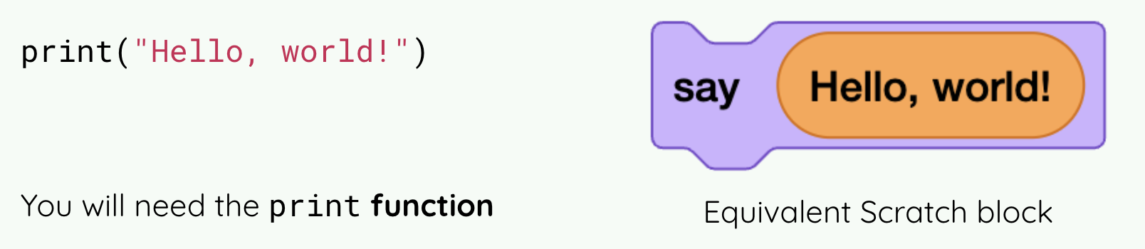
To solve the first problem, we decided that the initial lessons in the unit should start by showing familiar Scratch blocks right next to the equivalent Python syntax. This direct comparison makes the transition from block-based to text-based programmer smoother.
Comparison of Python syntax with equivalent Scratch block
To teach prompting, we built a gradual path. The unit starts with a debugging code activity, where students get code with errors and a prompt to make an LLM tool fix the errors. Later, they learn to break down a prompt into their goal (what output they want) and the context (additional information for the LLM tool). Eventually, they use a structured framework to prompt the tool to generate complete, bug-free code.
Handling the unpredictable outputs of LLM tools we turned into a learning activity. In one lesson, students are given different chatbot-generated code segments and asked to analyse and reflect on the code quality. This crucial exercise helps them build the critical thinking and code evaluation skills they need for programming with AI tools.
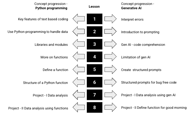
The progression of Python and generative AI concepts covered in the unit
Over the eight lessons, there is a progression of Python concepts and generative AI concepts, as shown in the image above. They lead students to complete two challenging, real-world data analysis projects.
Preparing the educators
To ensure the successful pilot of the ‘Programming with AI’ unit, a comprehensive teacher training program was essential. We understood that teachers needed confidence and competence not only in the subject matter — programming — but also in guiding students to ethically and effectively use LLM tools.
STEM and ICT teachers participated in the training
The training was an intensive, three-day programme: two days were held in-person for deep collaboration and one day was virtual for reinforcing key information. We covered five critical areas:
Hands-on activities to ensure comfort with the Python programming language
Exploring the capabilities and limitations of LLM tools
Effective prompt writing, which teachers would in turn model for their students to use for code debugging and idea generation
Reviewing lesson flow and learning objectives to understand the structure of a lesson
Adapting specific pedagogies to integrate an LLM tool in teaching the Python programming language
This training ensured our educators were not just teaching a new unit, but felt like confident facilitators ready to lead the shift towards AI-supported learning.
Initial student reactions: Excitement, familiarity with LLM tools, and seamless transition
The pilot of the ‘Programming with AI’ unit began during the second week of December 2025 across five selected schools. It was immediately met with enthusiastic student engagement — they were highly excited to learn Python programming using LLM tools.
When teachers initiated discussions about AI, students demonstrated their familiarity with LLMs, chatbots, and related concepts. They were not only aware of generative AI but could readily name and describe the functions of LLM tools, telling us they were actively using these tools to create projects in various other subjects.
Students could easily connect with the activities in the lessons as they had foundational understanding of programming, which they developed while learning block-based coding in Scratch. This prior knowledge enabled their seamless transition to the new learning. Perhaps most impressive was the students’ rapid adoption of LLM tools to debug their code. This skill can ease what is traditionally a steep learning curve when students first learn text-based programming.
We are now eagerly anticipating their curiosity and progress in the upcoming lessons.
Looking ahead and collecting impact data
With the initial enthusiasm confirmed, the pilot program moves into its next critical phase. Teachers will continue to deliver the unit over the next few months in the five selected schools in Telangana.
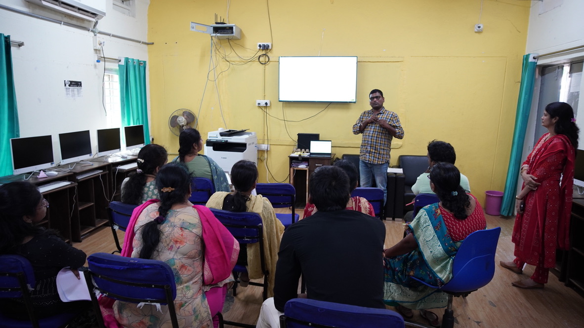
The teachers and team at our ‘Programming with AI’ training.
During this extended observation period, our primary focus will be on rigorous data collection and impact assessment. We will closely monitor how students interact with the provided learning materials and how they use LLM tools throughout the unit. We will systematically assess whether the new teaching approach successfully helps students achieve the defined learning objectives for Python programming. Crucially, we will capture comprehensive data to understand the impact of this AI-integrated approach on engagement, skill acquisition, and problem-solving compared to traditional methods.
Based on the synthesis and analysis of all the gathered data, we will share our gathered insights early next year. The findings will inform our plans for more widely introducing the AI-integrated unit and for developing similar content for other settings and age groups.
В „Тоест разговаряме“ със Светла Енчева обсъдихме многолюдните протести, довели до падането на правителството, споделихме вдъхновението от гражданската енергия, но и рационалните притеснения от възможностите за последващ „разцвет“ на евроскептични, антидемократични и проруски идеологии по унгарски/словашки модел.
Продължихме с темите, за които Светла пише в „Тоест“: правата на уязвимите и малцинствените групи, липсващата помощ за хората с деменция и техните близки, палиативните грижи за деца, интимния живот и достойнството на хората с увреждания, „женското лице“ на бедността, невидимите капани пред работещите майки и др. Светла говори за институционалната слепота и дехуманизацията, за хората, които „ги няма в списъка“, и за значението на личните истории, през които тези проблеми стават видими.
Засегнахме и правата на ЛГБТИ хората – включително нейната собствена биография и избора ѝ да не крие сексуалната си ориентация, цената на тази видимост и дългия списък с права, от които ЛГБТИ хората у нас са лишени. Говорихме и за медийната етика – от подхода „сълзичка – паричка“ до риалити формати като „Ергенът“, които нормализират насилие, унижение и сексизъм под маската на „забавление“.
Гледайте целия разговор в нашия YouTube канал:
Може да го чуете и като аудиозапис в SoundCloud:
На живо включихме и въпроси от публиката, но не успяхме пълноценно да отговорим на всички. Помолих Светла да допълни тук един от зрителските въпроси, а именно:
От какви основни права са лишени еднополовите двойки в България?
Освен от правата, произтичащи от конституционната забрана да сключват брак, и от тези, свързани с отглеждането на деца, хората в еднополови връзки в България умишлено биват лишавани и от други права. Едно от тях е правото на защита от домашно насилие – в Закона за защита от домашното насилие се прие дефиниция за интимна връзка, която включва само хетеросексуалните отношения. Така че според българското законодателство еднополовите двойки не само не можем да сключваме брак, а и връзките ни… не съществуват. Моята връзка например щастливо „не съществува“ вече 10 години.
Преди срещата ви помолихме да отговорите на кратката ни анкета. Ето и резултатите от нея:
Равните права са условие за достойно съществуване.
Светла Енчева е журналистка, редакторка и социоложка на свободна практика. Редовна авторка и редакторка е в „Тоест“, писала е и за „Свободна Европа“, „Маргиналия“ и други медии. Участвала е в множество изследователски проекти с фокус върху човешки права, уязвими групи, дискриминация, проблеми на жените и др. Завършила е философия, преподавала е социология и е активистка в областта на човешките права. Открито нехетеросексуална е и от 10 години е в щастлива връзка с жена.
Следващата среща на „Тоест разговаряме“ ще бъде с Йоанна Елми, която е дългогодишна авторка на „Тоест“ и поддържа бюлетина „Гласовете на Америка“. Разговорът ще се излъчва на живо в YouTube Liveна 17 януари, събота, от 16:00 ч.
В „Тоест разговаряме“ всеки месец ви срещаме с автори, които познавате добре от анализите или от рубриките им в „Тоест“, но този път ще ги видите и чуете в по-личен и непосредствен формат. Във видеоразговорите, предавани на живо, активно участие имате и вие, нашата публика – със своите въпроси, коментари и включване в тематичната анкета. Водещ на поредицата е Владислав Севов, дългогодишен телевизионен журналист и съосновател на „Тоест“.
„Тоест разговаряме“ е поредица, подкрепена от Институт „Отворено общество – София“ и съфинансирана от Европейския съюз в рамките на проекта Media Resilience. Изразените възгледи и мнения са само и изцяло на техните автори и не отразяват непременно възгледите и мненията на Европейския съюз, на Европейската изпълнителна агенция за образование и култура (EACEA) или на Институт „Отворено общество – София“ (ИООС). Нито Европейският съюз, нито EACEA, нито ИООС могат да бъдат държани отговорни за тях.
Delivering personalized user experiences in real-time is central to Grab’s strategy, but achieving this at scale poses significant engineering challenges. Grab’s Customer Data Platform (CDP) and Growth team has successfully delivered several real-time campaigns, driving significant business impact through enhanced personalization. These initiatives include high-impact use cases like immediate mall offers, timely traveler recommendations, precise ad retargeting, and proactive interventions during key user journey moments. At the core of these successes is Grab’s CDP, which rapidly deploys advanced real-time personalization via a powerful new capability called “Scenarios.”
About Grab’s CDP
Grab’s CDP is a centralized, reliable repository for user attributes, designed for freshness, governance, and reusability. Built on Grab’s Signal Marketplace framework, the CDP streamlines data management through automation and integration, supporting seamless interactions with internal services and toolings that power marketing, experimentation, ads, Machine Learning (ML) features, and external platforms, including Facebook, Google Ads, and TikTok.
The platform currently manages over 1,000 batch user attributes for Passengers, Drivers, and Merchants, powering diverse use cases from targeted marketing campaigns to operational decision-making across Grab’s entire ecosystem.
The need for real-time personalization
In our current CDP setup, user segments are primarily created for targeting using batch attributes that update once daily. While these batch updates provide valuable historical insights, they are not suitable for scenarios requiring real-time responsiveness. This delay prevents timely engagement with users, particularly when immediate actions can significantly enhance user experiences and conversion rates.
For example, when travelers land at an airport, they immediately benefit from timely suggestions for rides, dining options, or local attractions. Traditional batch processing cannot deliver the agility and responsiveness required for these dynamic scenarios.
Historically, real-time personalization at Grab relied heavily on engineering resources, which resulted in limited scalability and agility. Marketers and product teams often found themselves blocked by engineering bandwidth constraints, restricting experimentation and innovation.
Problem statement
The limitations of Grab’s existing personalization frameworks include:
Batch attribute delays: Daily updates are insufficient for scenarios requiring immediate user responses.
Limited dynamic enrichment: Difficulties in dynamically integrating real-time events with historical user data, weakens personalization effectiveness.
High engineering overhead: Custom solutions require extensive resources, limiting agility and innovation.
To overcome these challenges and support Grab’s vision for comprehensive personalization – including proactive recommendations and assistance – CDP needed robust real-time capabilities.
CDP Scenarios: Real-time personalization made simple
The Scenario feature revolutionizes real-time targeting within the CDP by utilizing user-initiated events, geo-fencing, historical profile data, and on-the-fly predictions. This empowers the business to deliver easy, quick, and flexible personalization without the need for complex engineering efforts.
Scenarios enable innovative use cases such as these:
Mall personalization: Real-time personalized offers upon arrival.
Traveler assistance: Immediate recommendations at airports or hotels.
Ad retargeting: Enhanced real-time ad targeting.
Conversion optimization: Timely intervention during user drop-off points.
Imagine predicting a user’s intent to drop off at a mall using both real-time and historical context. For instance, when a user books a ride to a mall, factors such as destination, time, cuisine preferences, and past behavior (e.g., affluence level) can help predict whether the user’s purpose is retail therapy, grocery shopping, or dining out. This prediction accounts for elements like time of day, day of the week, and mall location. Grab’s engineering teams can leverage this predicted intent (signal) to offer personalized actions, such as GrabPay discounts for shopping or exclusive dining offers for dinner.
Figure 1. Scenario in CDP.
Key features
Event-driven personalization: Real-time Scenarios triggered by Scribe events (Grab’s comprehensive event collection and tracking platform) combined with geo-fencing.
Historical context integration: Optionally enrich Scenarios using historical CDP data.
Predictive modeling: Deploy pre-trained models for instant user behavior predictions.
Self-serve graphical user interface (GUI): Enable marketers to create complex event sequences and validate Scenarios with synthetic data processed through Flink pipelines.
Headless application programming interfaces (APIs): Allow programmatic access and management of Scenarios.
Figure 2. Attributes for a scenario in CDP.
Self-serve Scenario creation
We designed an intuitive self-serve UI, embedded within the Grab app, empowering marketers to quickly define and deploy Scenarios. Users can specify event triggers, configure geo-fencing, incorporate historical user attributes, and select predictive models. Marketers can also validate Scenarios using synthetic data before deployment, ensuring accurate and realistic outcomes.
How it works:
Select event triggers: Choose predefined events or define custom intra-session sequences via the GUI.
Configure geo-fencing: Define Scenario activation locations, like airports or malls.
Include historical attributes (optional): Utilize batch attributes from the CDP to enrich Scenarios.
Select predictive models (optional): Train custom classifiers or pick from pre-trained Catwalk models.
Define data sink: Choose between Amphawa (DynamoDB), Kafka, or both; potentially extendable to external destinations (e.g., Appsflyer).
Once configured, metadata synchronizes automatically with our streaming service, and Scenarios become available for real-time consumption within an hour.
Proven impact: Real-world success
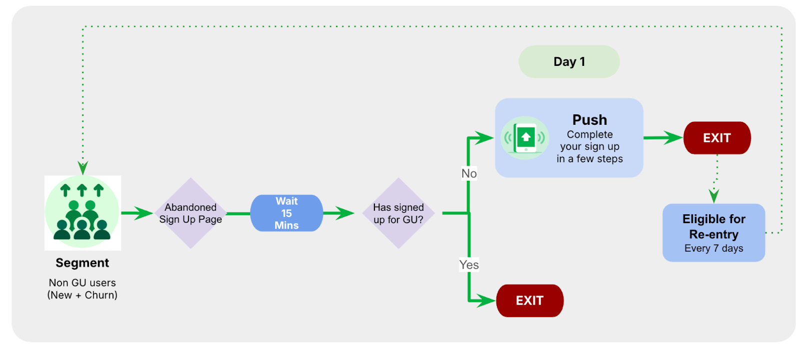
CDP Scenarios are already delivering measurable business results, with over 12 live production implementations. For instance, in a case study addressing Grab Unlimited subscription signup abandonment, we leveraged CDP Scenarios to increase signups by engaging users in real time within 15 minutes of them leaving the signup process.
Figure 3. Grab Unlimited sign-up journey.
To enhance conversion rates, personalized real-time nudges were deployed through Scenarios. For example, users who started the signup process but failed to complete it within 15 minutes received a follow-up notification, prompting them to finalize their registration.
Figure 4. Scenario flow for Grab Unlimited registration.
This scenario alone achieved more than a 3% uplift in subscriber conversions vs non-real-time acquisition campaigns, demonstrating Scenarios’ potential to significantly boost business outcomes.
Technical architecture: Low latency, high reliability
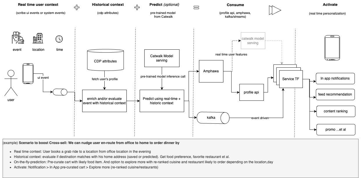
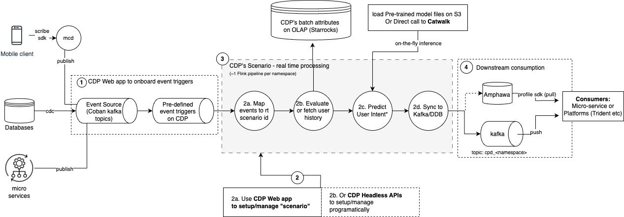
Figure 5. High-level scenario flow. Scenarios are designed for low latency (under 15 seconds) and high reliability.
Event registration: Popular UI events from Scribe are whitelisted and immediately available; custom events are onboarded via the CDP web portal.
Scenario creation: Users configure Scenarios through a user-friendly GUI, defining events, historical contexts, and predictive models.
Real-time Flink processing: Incoming events trigger Scenarios, evaluating user historical data via StarRocks and performing real-time predictions using pre-trained models.
Real-time data sync: Outcomes are synced back to Kafka or Amphawa (Grab’s internal feature store built on AWS DynamoDB), enriching data for use by subsequent services.
Consumption by downstream services: Kafka streams or CDP’s Profile SDK facilitates immediate, personalized user experiences.
Advancing the future of real-time personalization
As we continue to innovate, we are focused on enhancing the capabilities of CDP Scenarios to support more complex and scalable personalization use cases. Here are some key areas of improvement we are exploring:
Optimized Scenario sharding for scalable processing: To accommodate the growing number of use cases, we plan to scale and orchestrate our Flink pipeline fleet in a headless manner. This approach will improve system stability and enable seamless management of complex Scenarios across the pipeline.
Enhanced signal distribution across multiple destinations: Currently, Scenario outputs are limited to a single topic or sink. To address the increasing diversity of use cases, we aim to expand signal distribution, allowing downstream consumers to access Scenario outcomes through multiple scalable and reliable channels.
Advanced scheduling and delayed triggering: While real-time computation of Scenario signals is effective, certain use cases require delayed activation for maximum impact. We are exploring ways to compute signals instantly but trigger actions at scheduled times, such as sending a push notification for booking a return Grab ride based on the average wait time at the drop-off location.
The launch of CDP Scenarios represents a significant milestone for Grab, paving the way for scalable, efficient, and user-friendly real-time personalization. Initial successes have demonstrated its immense potential, delivering notable improvements in user engagement and conversion rates. Looking ahead, we are committed to continuously advancing Scenarios by expanding its features, integrations, and applications to further elevate user experiences across the Grab ecosystem.
Join us
Grab is a leading superapp in Southeast Asia, operating across the deliveries, mobility and digital financial services sectors. Serving over 800 cities in eight Southeast Asian countries, Grab enables millions of people everyday to order food or groceries, send packages, hail a ride or taxi, pay for online purchases or access services such as lending and insurance, all through a single app. Grab was founded in 2012 with the mission to drive Southeast Asia forward by creating economic empowerment for everyone. Grab strives to serve a triple bottom line – we aim to simultaneously deliver financial performance for our shareholders and have a positive social impact, which includes economic empowerment for millions of people in the region, while mitigating our environmental footprint.
Powered by technology and driven by heart, our mission is to drive Southeast Asia forward by creating economic empowerment for everyone. If this mission speaks to you, join our team today!
Front: Civil Infrastructure Platform; COSMIC desktop; Calibre adds AI; Maintainer’s Summit; ML tools for kernel development; linux-next; Rust in the kernel; kernel development tools; Linux process improvements; 6.19 merge window part 2.
Briefs: capsudo; Asahi Linux 6.18; Pop!_OS 24.04; Vojtux; KDE Gear 25.12; Rust 1.92.0; Quotes; …
Announcements: Newsletters, conferences, security updates, patches, and more.
A new version of AWS Security Hub is now generally available with new capabilities to aggregate, correlate, and contextualize your security alerts across Amazon Web Services (AWS) accounts. The prior version is now known as AWS Security Hub CSPM and will continue to be available as a unique service focused on cloud security posture management and finding aggregation.
One capability available in both services is automation rules. In both Security Hub and Security Hub CSPM, you can use automation rules to automatically update finding fields when the criteria they define are met. In Security Hub, automation rules can be used to send findings to third-party platforms for operational response. Many existing Security Hub CSPM users have automation rules for tasks such as elevating the severity of a finding because it affects a production resource or adding a comment to assist in remediation workflows. While both services offer similar automation rule functionality, rules aren’t synchronized across the two services. If you are an existing Security Hub CSPM customer looking to adopt the new Security Hub, you might be interested in migrating the automation rules that have already been built. This helps keep your automation rules processing close to where you’re reviewing findings. As of publication, this capability is included in the cost of the Security Hub essentials plan. For current pricing details, refer to the Security Hub pricing page.
This post provides a solution to automatically migrate automation rules from Security Hub CSPM to Security Hub, helping you maintain your security automation workflows while taking advantage of the new Security Hub features. If you aren’t currently using automation rules and want to get started, see Automation rules in Security Hub.
Automation rule migration challenge
Security Hub CSPM uses the AWS Security Finding Format (ASFF) as the schema for its findings. This schema is fundamental to how automation rules are applied to findings as they are generated. Automation rules begin by defining one or more criteria and then selecting one or more actions that will be applied when the specified criteria are met. Each criterion specifies an ASFF field, an operator (such as equals or contains), and a value. Actions then update one or more ASFF fields.
The new version of Security Hub uses the Open Cybersecurity Schema Framework (OCSF), a widely adopted open-source schema supported by AWS and partners in the cybersecurity industry. Security Hub automation rules structurally work the same way as Security Hub CSPM rules. However, the underlying schema change means existing automation rules require transformation.
The solution provided in this post automatically discovers Security Hub CSPM automation rules, transforms them into the OCSF schema, and creates an AWS CloudFormation template that you can use to deploy them to your AWS account running the new version of Security Hub. Because of inherent differences between the ASFF and OCSF schemas, some rules can’t be automatically migrated, while others might require manual review after migration.
The following table show the current mapping between ASFF fields supported as criteria and their corresponding OCSF fields. These mappings may change in future service releases. Fields marked as N/A can’t be migrated and will require special consideration when migrating automation rules. They need to be redesigned in the new Security Hub. The solution provided in this post is designed to skip migration of rules with one or more ASFF criteria that don’t map to an OCSF field but will identify those rules in a report for your review.
Rule criterion in ASFF
Corresponding OCSF field
AwsAccountId
cloud.account.uid
AwsAccountName
cloud.account.name
CompanyName
metadata.product.vendor_name
ComplianceAssociatedStandardsId
compliance.standards
ComplianceSecurityControlId
compliance.control
ComplianceStatus
compliance.status
Confidence
confidence_score
CreatedAt
finding_info.created_time
Criticality
N/A
Description
finding_info.desc
FirstObservedAt
finding_info.first_seen_time
GeneratorId
N/A
Id
finding_info.uid
LastObservedAt
finding_info.last_seen_time
NoteText
comment
NoteUpdatedAt
N/A
NoteUpdatedBy
N/A
ProductArn
metadata.product.uid
ProductName
metadata.product.name
RecordState
activity_name
RelatedFindingsId
N/A
RelatedFindingsProductArn
N/A
ResourceApplicationArn
N/A
ResourceApplicationName
N/A
ResourceDetailsOther
N/A
ResourceId
resources[x].uid
ResourcePartition
resources[x].cloud_partition
ResourceRegion
resources[x].region
ResourceTags
resources[x].tags
ResourceType
resources[x].type
SeverityLabel
vendor_attributes.severity
SourceUrl
finding_info.src_url
Title
finding_info.title
Type
finding_info.types
UpdatedAt
finding_info.modified_time
UserDefinedFields
N/A
VerificationState
N/A
WorkflowStatus
status
The following table shows the ASFF fields that are supported as actions and their corresponding OCSF fields. Note that several action fields aren’t available in OCSF:
Rule action fields in ASFF
Corresponding OCSF field
Confidence
N/A
Criticality
N/A
Note
Comment
RelatedFindings
N/A
Severity
Severity
Types
N/A
UserDefinedFields
N/A
VerificationState
N/A
Workflow Status
Status
For Security Hub CSPM automation rules that include actions without OCSF equivalents, the solution is designed to migrate the rules but include only the supported actions. These rules will be designated as partially migrated in the rule description and the migration report. You can use this information to review and modify the rules before enabling them, helping to ensure that the new automation rules behave as expected.
Solution overview
This solution provides a set of Python scripts designed to assist with the migration of automation rules from Security Hub CSPM to the new Security Hub. Here’s how the migration process works:
Begin migration: The solution provides an orchestration script that initiates three sub-scripts and manages passing the proper inputs to them.
Discovery: The solution scans your Security Hub CSPM environment to identify and collect existing automation rules across specified AWS Regions.
Analysis: Each rule is evaluated to determine if it can be fully migrated, partially migrated, or requires manual intervention based on ASFF to OCSF field mapping compatibility.
Transformation: Compatible rules are automatically converted from the ASFF schema to the OCSF schema using predefined field mappings.
Template creation: The solution generates a CloudFormation template containing the transformed rules, maintaining their original order and Regional context.
Deployment: Review the generated template and deploy it to create the migrated rules in Security Hub, where they are created in a disabled state by default.
Validate and enable rules: Review each migrated rule in the AWS Management Console for Security Hub to verify its criteria, actions, and preview your current matching findings if applicable. After confirming that the rules work as intended individually and as a sequence, enable them to resume your automation workflows.
Figure 1: Architecture diagram showing scripts and how they interact with AWS
The solution, shown in Figure 1, consists of four Python scripts that work together to migrate your automation rules:
Orchestrator: Coordinates discovery, transformation, and generation along with reporting and logging
Rule discovery: Identifies and extracts existing automation rules from Security Hub CSPM across the Regions you specify
Schema transformation: Converts the rules from ASFF to OCSF format using the field mapping detailed earlier
Template generation: Creates CloudFormation templates that you can use to deploy the migrate rules
Before running the solution, ensure you have the following components and permissions in place.
Required software:
AWS CLI (latest version)
Python 3.12 or later
Python packages:
boto3 (latest version)
pyyaml (latest version)
Required permissions: For rule discovery and transformation:
securityhub:ListAutomationRules
securityhub:BatchGetAutomationRules
securityhub:GetFindingAggregator
securityhub:DescribeHub
securityhub:ListAutomationRulesV2
For template deployment:
cloudformation:CreateStack
cloudformation:UpdateStack
cloudformation:DescribeStacks
cloudformation:CreateChangeSet
cloudformation:DescribeChangeSet
cloudformation:ExecuteChangeSet
cloudformation:GetTemplateSummary
securityhub:CreateAutomationRuleV2
securityhub:UpdateAutomationRuleV2
securityhub:DeleteAutomationRuleV2
securityhub:GetAutomationRuleV2
securityhub:TagResource
securityhub:ListTagsForResource
AWS account configuration
Security Hub supports a delegated administrator account model when used with AWS Organizations. This delegated administrator account centralizes the management of security findings and service configuration across your organization’s member accounts. Automation rules must be created in the delegated administrator account in the home Region, and in unlinked Regions. Member accounts can’t create their own automation rules.
We recommend using the same account as the delegated administrator for Security Hub CSPM and Security Hub to maintain consistent security management. Configure your AWS CLI with credentials for this delegated administrator account before running the migration solution (see Setting up the AWS CLI for more information).
While this solution is primarily designed for delegated administrator deployments, it also supports single-account Security Hub implementations.
Key migration concepts
Before proceeding with the migration of your automation rules from Security Hub CSPM to Security Hub, it’s important to understand several key concepts that affect how rules are migrated and deployed. These concepts influence the migration process and the resulting behavior of your rules. Understanding them will help you plan your migration strategy and validate the results effectively.
Default rule state
By default, migrated rules are created in a DISABLED state, meaning the actions will not be applied to findings as they are generated. The solution can optionally create rules in an ENABLED state, but this is not recommended. Instead, create the rules in a DISABLED state, review each rule, preview matching findings, and then move the rule to an ENABLED state when ready.
Unsupported fields
The migration report details any rules that can’t be migrated because they include one or more Security Hub CSPM criteria that aren’t supported by the new Security Hub. These cases occur because of the differences between the ASFF and OCSF schemas. These rules require special attention because they can’t be automatically replicated with equivalent behavior. This is particularly important if you have Security Hub CSPM rules that depend on priority order.
When rules have actions that aren’t supported, they will still be migrated if at least one action is supported. Rules with partially supported actions are flagged in the migration report and the new automation rule description and should be reviewed.
Home and linked Regions
Both Security Hub CSPM and Security Hub support a home Region that aggregates findings from linked Regions. However, their automation rules behave differently. Security Hub CSPM automation rules operate on a Regional basis. This means they only affect findings generated in the Region where they are created. Even if you use a home Region, Security Hub CSPM automation rules do not apply to the findings aggregated from linked Regions in the home Region. Security Hub supports automation rules defined in a home Region and applied to all linked Regions, and does not support the creation of automation rules in linked Regions. However, in Security Hub, unlinked Regions can still have their own automation rules that will affect only the findings generated in that Region. Unlinked Regions will need to have automation rules applied separately
The solution supports two deployment modes to handle these differences. The first mode, called Home Region, should be used for Security Hub deployments with a home Region enabled. This mode identifies Security Hub CSPM automation rules from specified Regions and then recreates them with an additional criteria to account for the Region the rule came from. Then, one CloudFormation template is generated that can be deployed in the home Region. The automation rules will still operate as intended because of the addition of the criteria for the original Region where it was created.
The second mode is called Region-by-Region. This mode is for users who don’t currently use a home Region. In this mode, the solution still discovers automation rules in the Regions specified but generates a unique CloudFormation template for each Region. The resulting templates can then be deployed one by one to the delegated administrator account for their corresponding Region. No additional criteria are added to the automation rule in this mode.
It is possible to use a home Region with Security Hub and link some Regions, but not all. If this is the case, run the Home Region mode for the home Region and all linked Regions. Then, re-run the solution in Region-by-Region mode for all unlinked Regions.
Rule order
Both Security Hub CSPM and Security Hub automation rules have an order in which they are evaluated. This can be important for certain situations where different automation rules might apply to the same findings or take actions on the same fields. This solution preserves the original order of your automation rules.
If there are existing Security Hub automation rules, the solution creates the new automation rules beginning after the existing rules. For example, if you have 3 Security Hub automation rules and are migrating 10 new rules, the solution will assign orders 4 through 13 to the new rules.
When using the Home Region mode, the order of automation rules for each Region is preserved and clustered together in the final order. For example, if a user with three Security Hub automation rules in three different Regions migrates the rules, they will be migrated sequentially. The solution will first migrate all rules from Region 1 in their original order, followed by all rules from Region 2 in their original order, and finally all rules from Region 3 in their original order.
Deploy and validate the migration
Now that you have the prerequisites in place and understand the basic concepts, you’re ready to deploy and validate the migration.
2. Run the scripts following the instructions of the README file, which will contain the most up-to-date implementation instructions. This will generate a CloudFormation template that will create the new Security Hub automation rules. Deploy the CloudFormation template using the AWS CLI or console. For more details, see the Create a stack from the CloudFormation console or the README file.
When deployment is complete, you can use the Security Hub console to review your migrated automation rules. Remember that rules are created in a DISABLED state by default. Review each rule’s criteria and actions carefully, checking that they match your intended automation workflow. You can also preview what existing findings would have matched each automation rule in the console.
To review and validate migrated rules:
1. Go to the Security Hub console and choose Automations from the navigation pane.
Figure 2: Security Hub Automations page
2. Select a rule and then choose Edit at the top of the page.
Figure 3: Security Hub automation rule details
3. Choose Preview matching findings. It’s possible that no findings will be returned even if the automation rule is behaving as expected. This means only that there are currently no findings matching the rule criteria in Security Hub. In this case, you can still review the rule criteria.
Figure 4: Security Hub Edit automation rule page
4. After validating a rule’s configuration, you can enable it through the console from the rule editing page. You can also update the CloudFormation stack. If you didn’t need to change any criteria or actions of your automation rules, you can re-run the scripts with the optional —create-enabled flag to reproduce the CloudFormation template with all rules enabled and deploy it as an update to the existing stack.
Pay attention to any rules that have partially migrated actions, which will be noted in the Description of each rule. This means one or more actions from the original rule in Security Hub CSPM aren’t supported in Security Hub and the rule might behave differently than intended. The solution also produces a migration report that includes which rules were partially migrated and specifies which actions from the original rule could not be migrated. Review these rules carefully because they might behave differently than expected and need to be modified or recreated.
Figure 5: Review the descriptions of partially migrated automation rules
Conclusion
The new AWS Security Hub provides enhanced capabilities for aggregating, correlating, and contextualizing your security findings. While the schema change from ASFF to OCSF brings improved interoperability and integration options, it requires existing automation rules to be migrated. The solution provided in this post helps automate this migration process through discovering your existing rules, transforming them to the new schema, and generating CloudFormation templates that preserve rule order and Regional context.
After migrating your automation rules, start by reviewing the migration report to identify any rules that weren’t fully migrated. Pay special attention to rules marked as partially migrated, because these might behave differently than their original versions. We recommend testing each rule in a disabled state and validating that rules work together as expected—especially rules that operate on the same fields—before enabling them in your environment.
To learn more about Security Hub and its enhanced capabilities, see the Security Hub User Guide. If you have feedback about this post, submit comments in the Comments section below.
A recently disclosed pair of vulnerabilities affecting Fortinet devices—CVE-2025-59718 and CVE-2025-59719—are drawing urgent attention after confirmation of their active exploitation in the wild. The vulnerabilities carry a critical CVSSv3 score and allow an unauthenticated remote attacker to bypass authentication using a crafted SAML message, ultimately gaining administrative access to the device. Current information indicates that the two CVEs have the same root cause and are differentiated by the products affected: CVE-2025-59719 specifically affects FortiWeb, while CVE-2025-59718 affects FortiOS, FortiProxy, and FortiSwitchManager.
While the vulnerable FortiCloud SSO feature is disabled by default in factory settings, it is automatically enabled when a device is registered to FortiCare via the GUI, unless an administrator explicitly opts out. This behavior significantly increases the likelihood of exposure across registered deployments. Arctic Wolf has confirmed active exploitation and CVE-2025-59718 was added to CISA’s Known Exploited Vulnerabilities (KEV) catalog on December 16.
Observed attacks show threat actors authenticating as the admin user and immediately downloading the system configuration file, which often contains hashed credentials. As a result, any organization with indicators of compromise must assume credential exposure and respond accordingly. A vendor patch is available, and organizations can also take immediate defensive action by disabling FortiCloud SSO administrative login while remediation efforts are underway.
Rapid7 observations
As of December 17, 2025, Rapid7 has observed CVE-2025-59718 exploitation attempts being performed against honeypots. Furthermore, a proof-of-concept exploit that resembles the observed honeypot requests has been posted to GitHub. These exploits are in the process of being validated against confirmed vulnerable targets.
Mitigation guidance
On December 9th, 2025, Fortinet published an advisory that outlines remediation steps for CVE-2025-59718 and CVE-2025-59719. According to Fortinet, the following versions are affected, and the fixed versions for each main release branch are also listed.
Fortinet’s advisory states that CVE-2025-59718 affects the following products and versions:
FortiOS
7.6 branch: versions 7.6.0 through 7.6.3 are affected, upgrade to 7.6.4 or above.
7.4 branch: versions 7.4.0 through 7.4.8 are affected, upgrade to 7.4.9 or above.
7.2 branch: versions 7.2.0 through 7.2.11 are affected, upgrade to 7.2.12 or above.
7.0 branch: versions 7.0.0 through 7.0.17 are affected, upgrade to 7.0.18 or above.
FortiProxy
7.6 branch: versions 7.6.0 through 7.6.3 are affected, upgrade to 7.6.4 or above.
7.4 branch: versions 7.4.0 through 7.4.10 are affected, upgrade to 7.4.11 or above.
7.2 branch: versions 7.2.0 through 7.2.14 are affected, upgrade to 7.2.15 or above.
7.0 branch: versions 7.0.0 through 7.0.21 are affected, upgrade to 7.0.22 or above.
FortiSwitchManager
7.2 branch: versions 7.2.0 through 7.2.6 are affected, upgrade to 7.2.7 or above.
7.0 branch: versions 7.0.0 through 7.0.5 are affected, upgrade to 7.0.6 or above.
Fortinet’s advisory states that CVE-2025-59719 affects the following product and versions:
FortiWeb
8.0 branch: version 8.0.0 is affected, upgrade to 8.0.1 or above.
7.6 branch: versions 7.6.0 through 7.6.4 are affected, upgrade to 7.6.5 or above.
7.4 branch: versions 7.4.0 through 7.4.9 are affected, upgrade to 7.4.10 or above.
Exposure Command, InsightVM, and Nexpose customers can assess their exposure to CVE-2025-59718 and CVE-2025-59719 with vulnerability checks expected to be available in the December 17 content release.
After three years of development, Linux hardware provider System76
has declared
the COSMIC desktop
environment stable. It shipped COSMIC Epoch 1 as part of the
long-awaited Pop!_OS 24.04 LTS
release on December 11, just in time for Linux enthusiasts to
have something to tinker with over the end-of-year holidays. With the
stable release out the door, it seemed like a good time to check back
in on COSMIC and see how it has evolved since the first alpha. For a first
stable release of a new desktop environment, COSMIC shows a lot of
promise and room to grow.
Following disclosure of the React2Shell vulnerability (CVE-2025-55182), a maximum-severity Remote Code Execution (RCE) in React Server Components (RSC) a.k.a. the Flight protocol, security teams are assessing exposure and validating fixes. React and ecosystem vendors have released patches; exploitation in the wild has been reported, so rapid validation matters.
What is React2Shell?
React2Shell is an unauthenticated RCE flaw caused by insecure Flight payload deserialization in server-side React/RSC implementations (including popular frameworks like Next.js). It carries a CVSS 10.0 rating and affects React versions 19.0.0, 19.1.0, 19.1.1, and 19.2.0 as well as Next.js versions 15.0.0-15.1.6 and 16.0.0-16.0.6 prior to recent patches. You can read more about it in this detailed CVE overview blog post.
In this detailed writeup, we will share how our customers can specifically test for React2Shell with Rapid7’s Application Security solution.
Testing for React2Shell with application security
With our dynamic application security testing (DAST) solution, customers can assess the risk of their applications. Rapid7 allows you to configure various attacks of your applications to identify response behaviors that make your applications more vulnerable to attacks. These attacks are run during scans that you can customize based on your needs. In this case, we’ve extended our RCE attack module to include a check for React2Shell.
What does this mean? Customers can now run an Attack Injection using the RCE, which includes an attack type for React2Shell. Our React2Shell vulnerability detection will simulate an attacker on your website. This is a benign attack which will not execute any code and only shows that RCE is possible. Rapid7 will validate the exploitability of the application and the associated risk.
How to run a React2Shell attack in the Rapid7 DAST
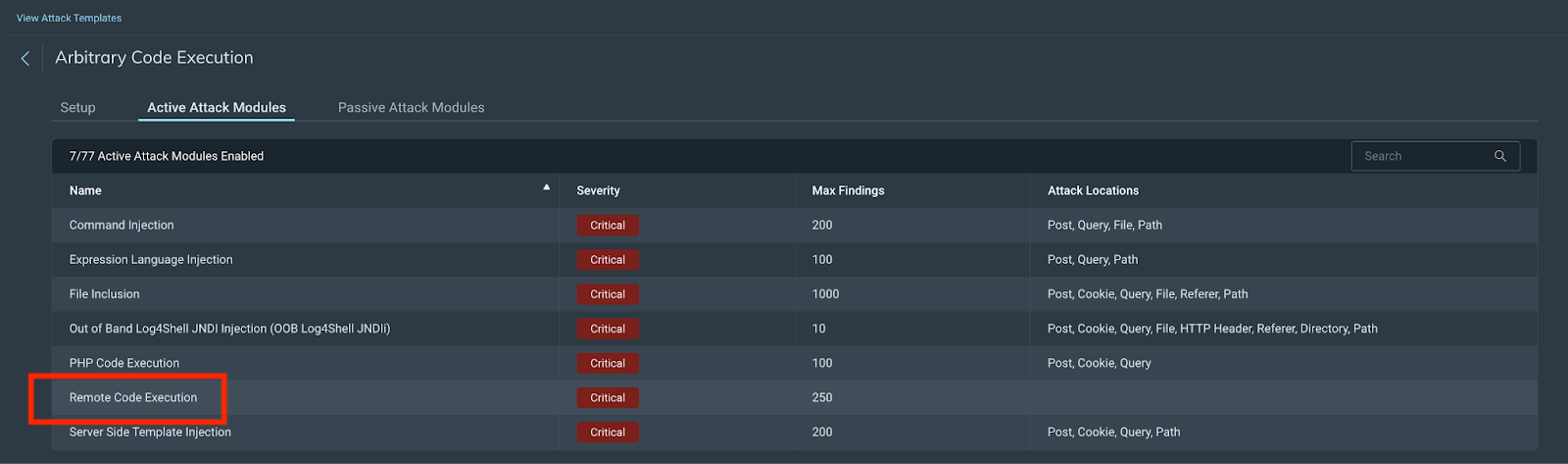
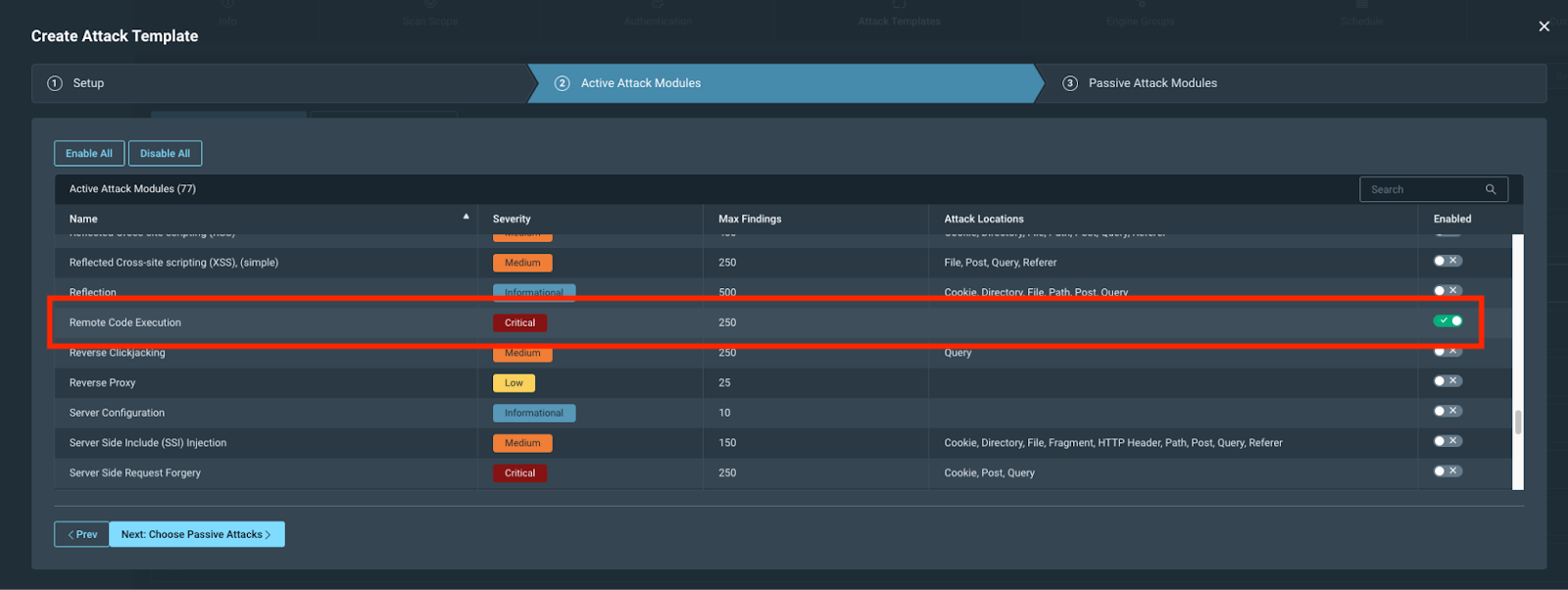
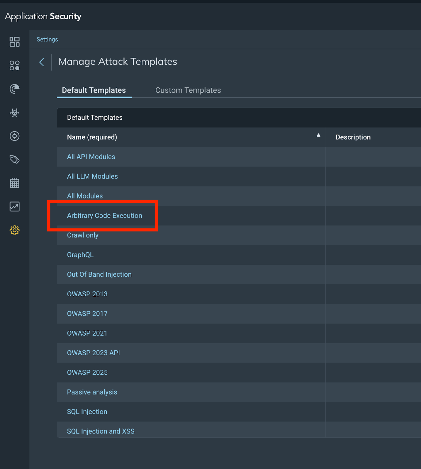
You can scan for this new RCE attack using either the new Arbitrary Code Execution attack template we have created or by creating your own custom attack template and selecting the RCE module. We have added some steps for you to follow below:
Default attack template option:
Choose the Arbitrary Code Execution attack template in your scan configuration:
⠀
Default Arbitrary Code Execution attack template with RCE attack module
Custom attack template option:
Custom Attack Template with RCE module
Run a scan
Choosing the scan configuration you made earlier, scan against your selected app(s).
Scan results – React2Shell RCE finding
Now that you have run your scan, you can review the results to see if your app(s) have any findings. These will include remediation advice that you can follow.
⠀
Manage attack templates
You can now manage your attack templates by navigating to the appropriate section and selecting the Arbitrary Code Execution attack template as below.
⠀
Manage attack templates
What’s next?
Patch immediately, upgrade React to 19.0.1, 19.1.2, or 19.2.1 (or newer). For Next.js, the recommended action is to update to the following respective patched versions: 15.2.6, 15.3.6, 15.4.8, 15.5.7, 16.0.7, or later*. You should seek to remediate this vulnerability on an urgent basis, outside of normal patch cycles and consider temporary web application firewall (WAF) rules for Flight endpoints while patching. If you’re looking to validate any fixes you have implemented, feel free to run a validation scan with our application security tool to verify the fixes are correct.
* For Next.js, the recommendation from Nextjs is to update to the following respective patched versions: 15.0.5, 15.1.9, 15.2.6, 15.3.6, 15.4.8, 15.5.7, 16.0.7, or later. However, we have identified that versions 15.0.5 and 15.1.9 have a different critical vulnerability and would recommend against using them.
Amazon Data Firehose supports Splunk Enterprise and Splunk Cloud as a delivery destination. This native integration between Splunk Enterprise, Splunk Cloud, and Amazon Data Firehose is designed to make AWS data ingestion setup seamless, while offering a secure and fault-tolerant delivery mechanism. We want to enable customers to monitor and analyze machine data from any source and use it to deliver operational intelligence and optimize IT, security, and business performance.
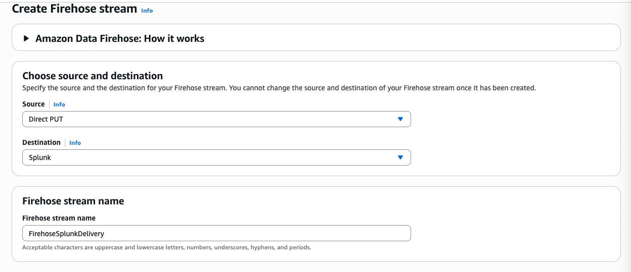
With Amazon Data Firehose, customers can use a fully managed, reliable, and scalable data streaming solution to Splunk. In this post, we tell you a bit more about the Amazon Data Firehose and Splunk integration. We also show you how to ingest large amounts of data into Splunk using Amazon Data Firehose.
Push vs. Pull data ingestion
Presently, customers use a combination of two ingestion patterns, primarily based on data source and volume, in addition to existing company infrastructure and expertise:
Push-based approach: Streaming data directly from AWS to Splunk HTTP Event Collector (HEC) by using Amazon Data Firehose. Examples of applicable data sources include CloudWatch Logs and Amazon Kinesis Data Streams.
The pull-based approach offers data delivery guarantees such as retries and checkpointing out of the box. However, it requires more ops to manage and orchestrate the dedicated pollers, which are commonly running on Amazon EC2 instances. With this setup, you pay for the infrastructure even when it’s idle.
On the other hand, the push-based approach offers a low-latency scalable data pipeline made up of serverless resources like Amazon Data Firehose sending directly to Splunk indexers (by using Splunk HEC). This approach translates into lower operational complexity and cost. However, if you need guaranteed data delivery then you have to design your solution to handle issues such as a Splunk connection failure or Lambda execution failure. To do so, you might use, for example, AWS Lambda Dead Letter Queues.
How about getting the best of both worlds?
Let’s go over the new integration’s end-to-end solution and examine how Amazon Data Firehose and Splunk together expand the push-based approach into a native AWS solution for applicable data sources.
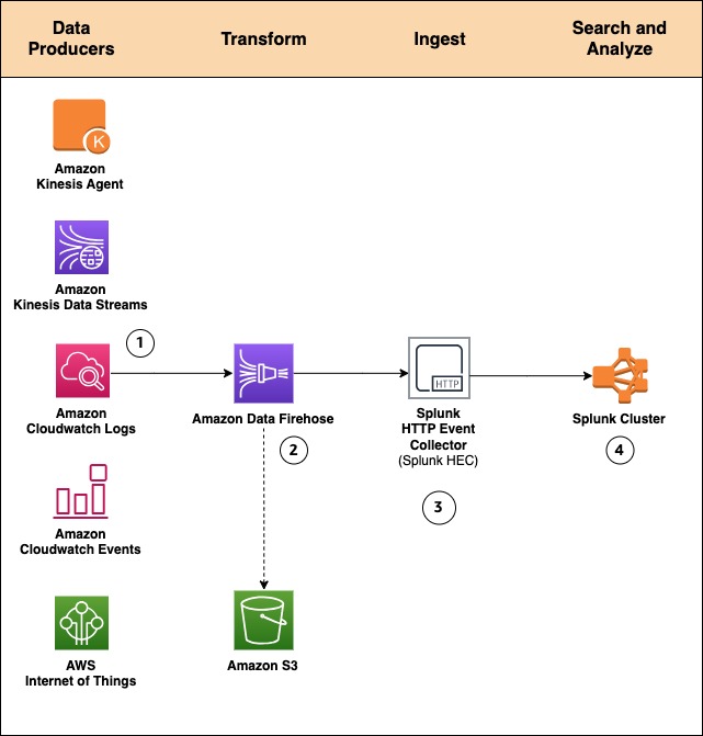
By using a managed service like Amazon Data Firehose for data ingestion into Splunk, we provide out-of-the-box reliability and scalability. One of the pain points of the old approach was the overhead of managing the data collection nodes (Splunk heavy forwarders). With the new Amazon Data Firehose to Splunk integration, there are no forwarders to manage or set up. Data producers (1) are configured through the AWS Management Console to drop data into Amazon Data Firehose.
You can also create your own data producers. For example, you can drop data into a Firehose delivery stream by using Amazon Kinesis Agent, or by using the Firehose API (PutRecord(), PutRecordBatch()), or by writing to a Kinesis Data Stream configured to be the data source of a Firehose delivery stream. For more details, refer to Sending Data to an Amazon Data Firehose Delivery Stream.
You might need to transform the data before it goes into Splunk for analysis. For example, you might want to enrich it or filter or anonymize sensitive data. You can do so using AWS Lambda and enabling data transformation in Amazon Data Firehose. In this scenario, Amazon Data Firehose is used to decompress the Amazon CloudWatch logs by enabling the feature.
Systems fail all the time. Let’s see how this integration handles outside failures to guarantee data durability. In cases when Amazon Data Firehose can’t deliver data to the Splunk Cluster, data is automatically backed up to an S3 bucket. You can configure this feature while creating the Firehose delivery stream (2). You can choose to back up all data or only the data that’s failed during delivery to Splunk.
In addition to using S3 for data backup, this Firehose integration with Splunk supports Splunk Indexer Acknowledgments to guarantee event delivery. This feature is configured on Splunk’s HTTP Event Collector (HEC) (3). It ensures that HEC returns an acknowledgment to Amazon Data Firehose only after data has been indexed and is available in the Splunk cluster (4).
Now let’s look at a hands-on exercise that shows how to forward VPC flow logs to Splunk.
How-to guide
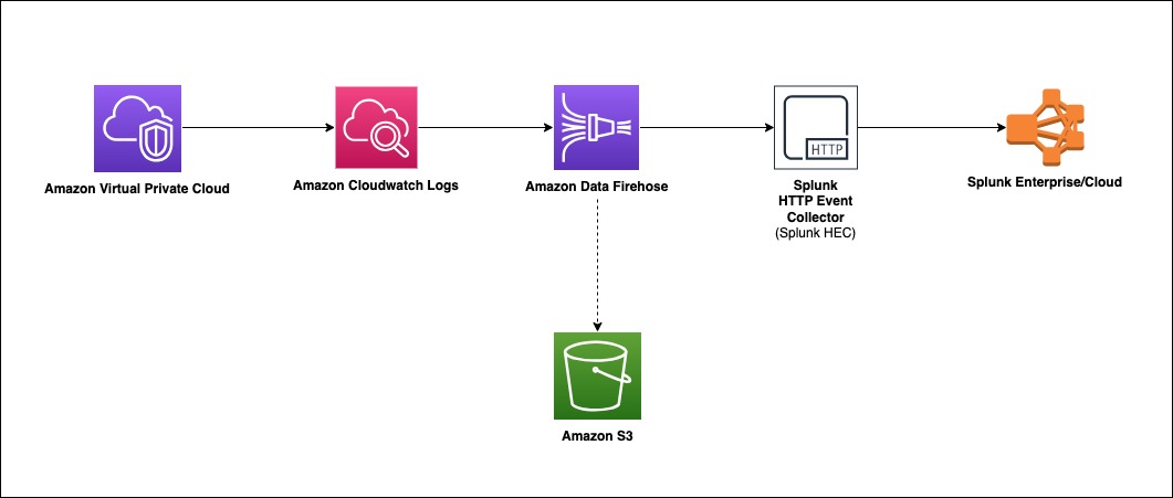
To process VPC flow logs, we implement the following architecture.
Amazon Virtual Private Cloud (Amazon VPC) delivers flow log files into an Amazon CloudWatch Logs group. Using a CloudWatch Logs subscription filter, we set up real-time delivery of CloudWatch Logs to an Amazon Data Firehose stream.
Data coming from CloudWatch Logs is compressed with gzip compression. To work with this compression, we will enable decompression for the Firehose stream. Firehose then delivers the raw logs to the Splunk Http Event Collector (HEC).
If delivery to the Splunk HEC fails, Firehose deposits the logs into an Amazon S3 bucket. You can then ingest the events from S3 using an alternate mechanism such as a Lambda function.
When data reaches Splunk (Enterprise or Cloud), Splunk parsing configurations (packaged in the Splunk Add-on for Amazon Data Firehose) extract and parse all fields. They make data ready for querying and visualization using Splunk Enterprise and Splunk Cloud.
Walkthrough
Install the Splunk Add-on for Amazon Data Firehose
The Splunk Add-on for Amazon Data Firehose enables Splunk (be it Splunk Enterprise, Splunk App for AWS, or Splunk Enterprise Security) to use data ingested from Amazon Data Firehose. Install the Add-on on all the indexers with an HTTP Event Collector (HEC). The Add-on is available for download from Splunkbase. For troubleshooting assistance, please refer to: AWS Data Firehose troubleshooting documentation & Splunk’s official troubleshooting guide
HTTP Event Collector (HEC)
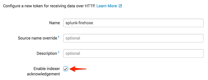
Before you can use Amazon Data Firehose to deliver data to Splunk, set up the Splunk HEC to receive the data. From Splunk web, go to the Setting menu, choose Data Inputs, and choose HTTP Event Collector. Choose Global Settings, ensure All tokens is enabled, and then choose Save. Then choose New Token to create a new HEC endpoint and token. When you create a new token, make sure that Enable indexer acknowledgment is checked.
When prompted to select a source type, select aws:cloudwatchlogs:vpcflow
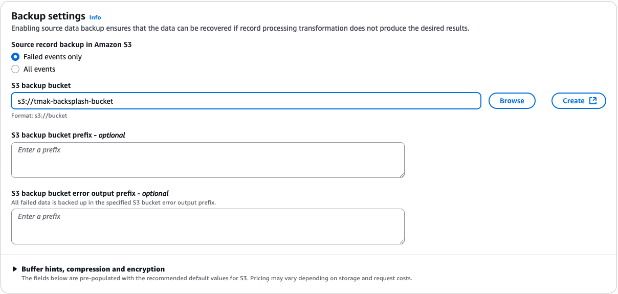
Create an S3 backsplash bucket
To provide for situations in which Amazon Data Firehose can’t deliver data to the Splunk Cluster, we use an S3 bucket to back up the data. You can configure this feature to back up all data or only the data that’s failed during delivery to Splunk.
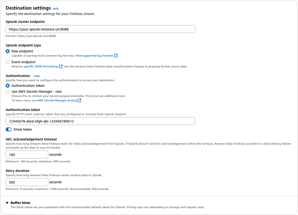
Enter your Splunk HTTP Event Collector (HEC) information in destination settings
Note: Amazon Data Firehose requires the Splunk HTTP Event Collector (HEC) endpoint to be terminated with a valid CA-signed certificate matching the DNS hostname used to connect to your HEC endpoint. You receive delivery errors if you are using a self-signed certificate.
In this example, we only back up logs that fail during delivery.
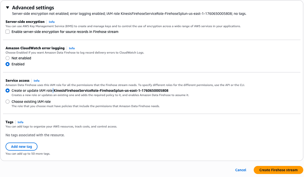
To monitor your Firehose delivery stream, enable error logging. Doing this means that you can monitor record delivery errors. Create an IAM role for the Firehose stream by choosing Create new, or Choose existing IAM role.
You now get a chance to review and adjust the Firehose stream settings. When you are satisfied, choose Create Firehose Stream.
Create a VPC Flow Log
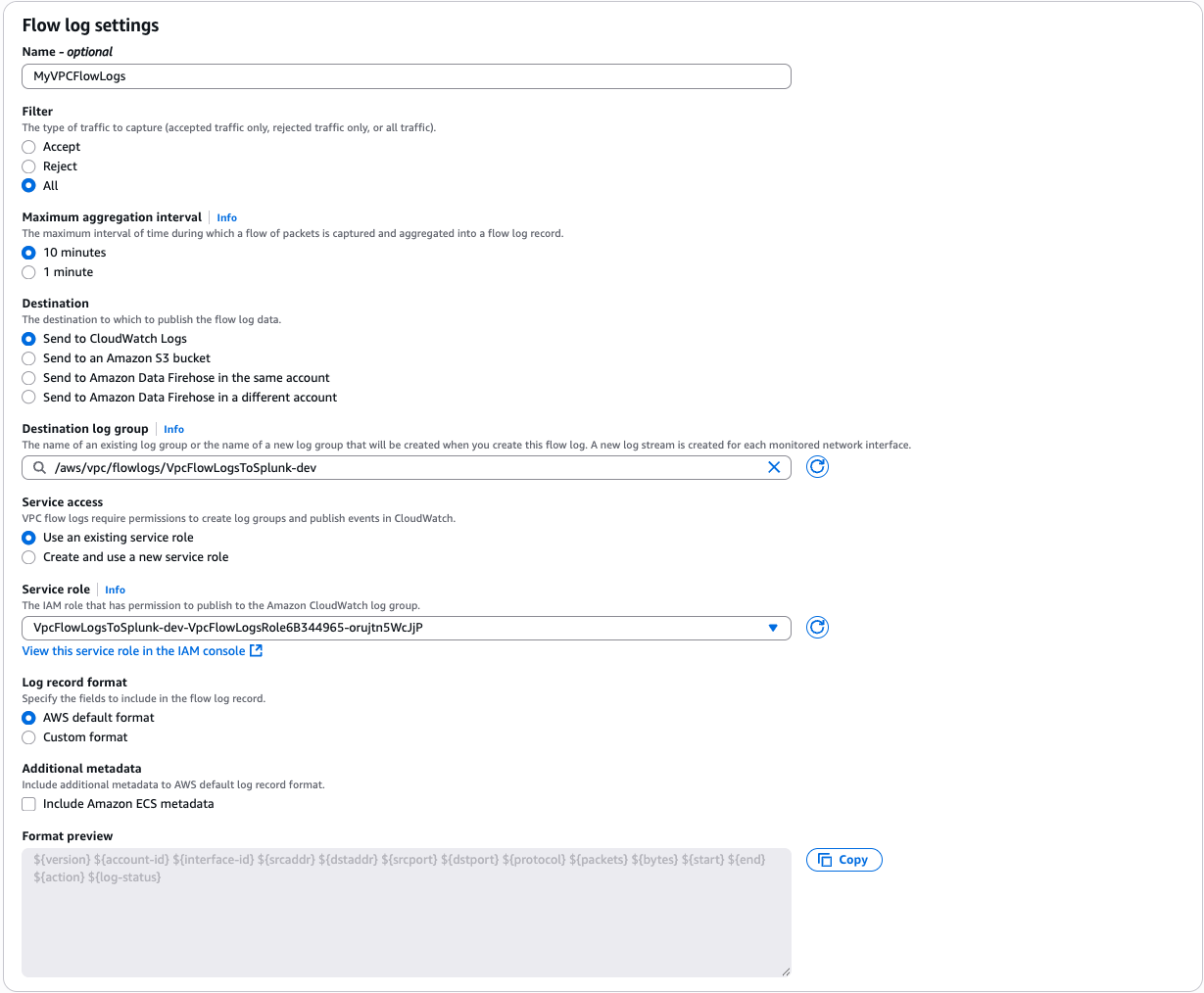
To send events from Amazon VPC, you need to set up a VPC flow log. If you already have a VPC flow log you want to use, you can skip to the “Publish CloudWatch to Amazon Data Firehose” section.
On the AWS console, open the Amazon VPC service. Then choose VPC, and choose the VPC you want to send flow logs from. Choose Flow Logs, and then choose Create Flow Log. If you don’t have an IAM role that allows your VPC to publish logs to CloudWatch, choose Create and use a new service role.
Once active, your VPC flow log should look like the following.
Publish CloudWatch to Amazon Data Firehose
When you generate traffic to or from your VPC, the log group is created in Amazon CloudWatch. We create an IAM role to allow Cloudwatch to publish logs to the Amazon Data Firehose Stream.
To allow CloudWatch to publish to your Firehose stream, you need to give it permissions.
$ aws iam create-role --role-name CWLtoFirehoseRole --assume-role-policy-document file://TrustPolicyForCWLToFireHose.json
Here is the content for TrustPolicyForCWLToFireHose.json.
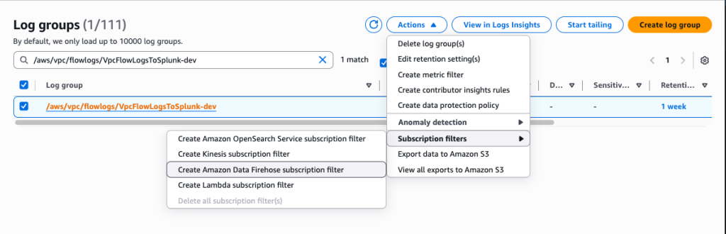
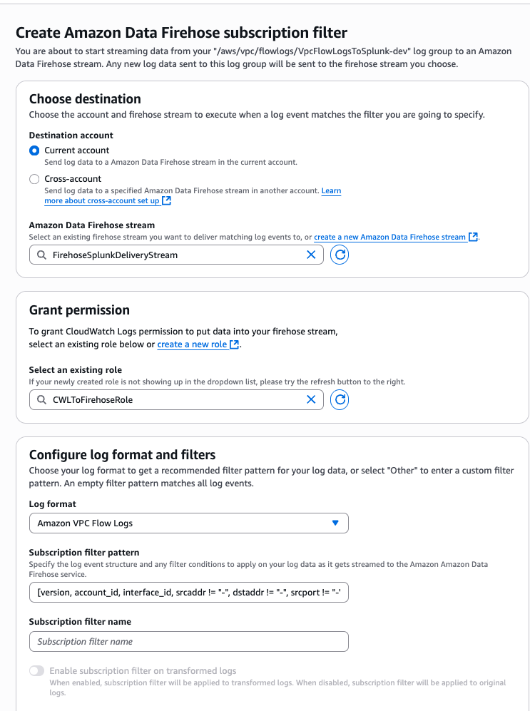
The new log group has no subscription filter, so set up a subscription filter. Setting this up establishes a real-time data feed from the log group to your Firehose delivery stream. Select the VPC flow log and choose Actions. Then choose Subscription filters followed by Create Amazon Data Firehose subscription filter.
When you run the AWS CLI command preceding, you don’t get any acknowledgment. To validate that your CloudWatch Log Group is subscribed to your Firehose stream, check the CloudWatch console.
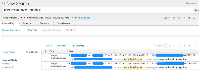
As soon as the subscription filter is created, the real-time log data from the log group goes into your Firehose delivery stream. Your stream then delivers it to your Splunk Enterprise or Splunk Cloud environment for querying and visualization. The screenshot following is from Splunk Enterprise.
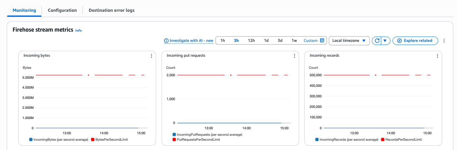
In addition, you can monitor and view metrics associated with your delivery stream using the AWS console.
Conclusion
Although our walkthrough uses VPC Flow Logs, the pattern can be used in many other scenarios. These include ingesting data from AWS IoT, other CloudWatch logs and events, Kinesis Streams or other data sources using the Kinesis Agent or Kinesis Producer Library. You may use a Lambda blueprint or disable record transformation entirely depending on your use case. For an additional use case using Amazon Data Firehose, check out This is My Architecture Video, which discusses how to securely centralize cross-account data analytics using Kinesis and Splunk.
Apache Iceberg is an open table format that helps combine the benefits of using both data warehouse and data lake architectures, giving you choice and flexibility for how you store and access data. See Using Apache Iceberg on AWS for a deeper dive on using AWS Analytics services for managing your Apache Iceberg data. Amazon Redshift supports querying Iceberg tables directly, whether they’re fully-managed using Amazon S3 Tables or self-managed in Amazon S3. Understanding best practices for how to architect, store, and query Iceberg tables with Redshift helps you meet your price and performance targets for your analytical workloads.
In this post, we discuss the best practices that you can follow while querying Apache Iceberg data with Amazon Redshift
1. Follow the table design best practices
Selecting the right data types for Iceberg tables is important for efficient query performance and maintaining data integrity. It is important to match the data types of the columns to the nature of the data they store, rather than using generic or overly broad data types.
Why follow table design best practices?
Optimized Storage and Performance: By using the most appropriate data types, you can reduce the amount of storage required for the table and improve query performance. For example, using the DATE data type for date columns instead of a STRING or TIMESTAMP type can reduce the storage footprint and improve the efficiency of date-based operations.
Improved Join Performance: The data types used for columns participating in joins can impact query performance. Certain data types, such as numeric types (such as, INTEGER, BIGINT, DECIMAL), are generally more efficient for join operations compared to string-based types (such as, VARCHAR, TEXT). This is because numeric types can be easily compared and sorted, leading to more efficient hash-based join algorithms.
Data Integrity and Consistency: Choosing the correct data types helps with data integrity by enforcing the appropriate constraints and validations. This reduces the risk of data corruption or unexpected behavior, especially when data is ingested from multiple sources.
How to follow table design best practices?
Leverage Iceberg Type Mapping: Iceberg has built-in type mapping that translates between different data sources and the Iceberg table’s schema. Understand how Iceberg handles type conversions and use this knowledge to define the most appropriate data types for your use case.
Select the smallest possible data type that can accommodate your data. For example, use INT instead of BIGINT if the values fit within the integer range, or SMALLINT if they fit even smaller ranges.
Utilize fixed-length data types when data length is consistent. This can help with predictable and faster performance.
Choose character types like VARCHAR or TEXT for text, prioritizing VARCHAR with an appropriate length for efficiency. Avoid over-allocating VARCHAR lengths, which can waste space and slow down operations.
Match numeric precision to your actual requirements. Using unnecessarily high precision (such as, DECIMAL(38,20) instead of DECIMAL(10,2) for currency) demands more storage and processing, leading to slower query execution times for calculations and comparisons.
Employ date and time data types (such as, DATE, TIMESTAMP) rather than storing dates as text or numbers. This optimizes storage and allows for efficient temporal filtering and operations.
Opt for boolean values (such as, BOOLEAN) instead of using integers to represent true/false states. This saves space and potentially enhances processing speed.
If the column will be used in join operations, favor data types that are typically used for indexing. Integers and date/time types generally allow for faster searching and sorting than larger, less efficient types like VARCHAR(MAX).
2. Partition your Apache Iceberg table on columns that are most frequently used in filters
When working with Apache Iceberg tables in conjunction with Amazon Redshift, one of the most effective ways to optimize query performance is to partition your data strategically. The key principle is to partition your Iceberg table based on columns that are most frequently used in query filters. This approach can significantly improve query efficiency and reduce the amount of data scanned, leading to faster query execution and lower costs.
Why partitioning Iceberg tables matters?
Improved Query Performance: When you partition on columns commonly used in WHERE clauses, Amazon Redshift can eliminate irrelevant partitions, reducing the amount of data it needs to scan. For example, if you have a sales table partitioned by date and you run a query to analyze sales data for January 2024, Amazon Redshift will only scan the January 2024 partition instead of the entire table. This partition pruning can dramatically improve query performance—in this scenario, if you have five years of sales data, scanning just one month means examining only 1.67% of the total data, potentially reducing query execution time from minutes to seconds.
Reduced Scan Costs: By scanning less data, you can lower the computational resources required and, consequently the associated costs.
Better Data Organization: Logical partitioning helps in organizing data in a way that aligns with common query patterns, making data retrieval more intuitive and efficient.
How to partition Iceberg tables?
Analyze your workload to determine which columns are most frequently used in filter conditions. For example, if you always filter your data for the last 6months, then that date will be a good partition key.
Select columns that have high cardinality but not too high to avoid creating too many small partitions. Good candidates often include:
Date or timestamp columns (such as, year, month, day)
Categorical columns with a moderate number of distinct values (such as, region, product category)
Define Partition Strategy: Use Iceberg’s partitioning capabilities to define your strategy. For example if you are using Amazon Athena to create a partitioned Iceberg table, you can use the following syntax.
CREATE TABLE iceberg_db.my_table ( id INT, date DATE, region STRING, sales DECIMAL(10,2) )
PARTITIONED BY (date, region)
LOCATION 's3://amzn-s3-demo-bucket/your-folder/'
TBLPROPERTIES ( 'table_type' = 'ICEBERG' )
Ensure your Redshift queries take advantage of the partitioning scheme by including partition columns in the WHERE clause whenever possible.
Walk-through with a sample usecase Let’s take an example to understand how to pick the best partition key by following best practices. Consider an e-commerce company looking to optimize their sales data analysis using Apache Iceberg tables with Amazon Redshift. The company maintains a table called sales_transactions, which has data for 5 years across four regions (North America, Europe, Asia, and Australia) with five product categories (Electronics, Clothing, Home & Garden, Books, and Toys). The dataset includes key columns such as transaction_id, transaction_date, customer_id, product_id, product_category, region, and sale_amount.
The data science team uses transaction_date and region columns frequently in filters, while product_category is used less frequently. The transaction_date column has high cardinality (one value per day), region has low cardinality (only 4 distinct values) and product_category has moderate cardinality (5 distinct values).
Based on this analysis, an effective partition strategy would be to partition by year and month from the transaction_date, and by region. This creates a manageable number of partitions while improving the most common query patterns. Here’s how we could implement this strategy using Amazon Athena:
3. Optimize by selecting only the necessary columns for query
Another best practice for working with Iceberg tables is to only select the columns that are necessary for a given query, and to avoid using the SELECT * syntax.
Why should you select only necessary columns?
Improved Query Performance: In analytics workloads, users typically analyze subsets of data, performing large-scale aggregations or trend analyses. To optimize these operations, analytics storage systems and file formats are designed for efficient column-based reading. Examples include columnar open file formats like Apache Parquet and columnar databases such as Amazon Redshift. A key best practice to select only the required columns in your queries, so the query engine can reduce the amount of data that needs to be processed, scanned, and returned. This can lead to significantly faster query execution times, especially for large tables.
Reduced Resource Utilization: Fetching unnecessary columns consumes additional system resources, such as CPU, memory, and network bandwidth. Limiting the columns selected can help optimize resource utilization and improve the overall efficiency of the data processing pipeline.
Lower Data Transfer Costs: When querying Iceberg tables stored in cloud storage (e.g., Amazon S3), the amount of data transferred from the storage service to the query engine can directly impact the data transfer costs. Selecting only the required columns can help minimize these costs.
Better Data Locality: Iceberg partitions data based on the values in the partition columns. By selecting only the necessary columns, the query engine can better leverage the partitioning scheme to improve data locality and reduce the amount of data that needs to be scanned.
How to only select necessary columns?
Identify the Columns Needed: Carefully analyze the requirements of each query and determine the minimum set of columns required to fulfill the query’s purpose.
Use Selective Column Names: In the SELECT clause of your SQL queries, explicitly list the column names you need, rather than using SELECT *.
4. Generate AWS Glue data catalog column level statistics
Table statistics play an important role in database systems that utilize Cost-Based Optimizers (CBOs), such as Amazon Redshift. They help the CBO make informed decisions about query execution plans. When a query is submitted to Amazon Redshift, the CBO evaluates multiple possible execution plans and estimates their costs. These cost estimates heavily depend on accurate statistics about the data, including: Table size (number of rows), column value distributions, Number of distinct values in columns, Data skew information, and more.
AWS Glue Data Catalog supports generating statistics for data stored in the data lake including for Apache Iceberg. The statistics include metadata about the columns in a table, such as minimum value, maximum value, total null values, total distinct values, average length of values, and total occurrences of true values. These column-level statistics provide valuable metadata that helps optimize query performance and improve cost efficiency when working with Apache Iceberg tables.
Why generating AWS Glue statistics matter?
Amazon Redshift can generate better query plans using column statistics, thereby improve performance on queries due to optimized join orders, better predicate push-down and more accurate resource allocation.
Costs will be optimized. Better execution plans lead to reduced data scanning, more efficient resource utilization and overall lower query costs.
How to generate AWS Glue statistics?
The Sagemaker Lakehouse Catalog enables you to generate statistics automatically for updated and created tables with a one-time catalog configuration. As new tables are created, the number of distinct values (NDVs) are collected for Iceberg tables. By default, the Data Catalog generates and updates column statistics for all columns in the tables on a weekly basis. This job analyzes 50% of records in the tables to calculate statistics.
On the Lake Formation console, choose Catalogs in the navigation pane.
Select the catalog that you want to configure, and choose Edit on the Actions menu.
You can override the defaults and customize statistics collection at the table level to meet specific needs. For frequently updated tables, statistics can be refreshed more often than weekly. You can also specify target columns to focus on those most commonly queried. You can set what percentage of table records to use when calculating statistics. Therefore, you can increase this percentage for tables that need more precise statistics, or decrease it for tables where a smaller sample is sufficient to optimize costs and statistics generation performance.These table-level settings can override the catalog-level settings previously described.
5. Implement Table Maintenance Strategies for Optimal Performance
Over time, Apache Iceberg tables can accumulate various types of metadata and file artifacts that impact query performance and storage efficiency. Understanding and managing these artifacts is crucial for maintaining optimal performance of your data lake. As you use Iceberg tables, three main types of artifacts accumulate:
Small Files: When data is ingested into Iceberg tables, especially through streaming or frequent small batch updates, many small files can accumulate because each write operation typically creates new files rather than appending to existing ones.
Deleted Data Artifacts: Iceberg uses copy-on-write for updates and deletes. When records are deleted, Iceberg creates “delete markers” rather than immediately removing the data. These markers need to be processed during reads to filter out deleted records.
Snapshots: Every time you make changes to your table (insert, update, or delete data), Iceberg creates a new snapshot—essentially a point-in-time view of your table. While valuable for maintaining history, these snapshots increase metadata size over time, impacting query planning and execution.
Unreferenced Files: These are files that exist in storage but aren’t linked to any current table snapshot. They occur in two main scenarios:
When old snapshots are expired, the files exclusively referenced by those snapshots become unreferenced
When write operations are interrupted or fail midway, creating data files that aren’t properly linked to any snapshot
Why table maintenance matters?
Regular table maintenance delivers several important benefits:
Enhanced Query Performance: Consolidating small files reduces the number of file operations required during queries, while removing excess snapshots and delete markers streamlines metadata processing. These optimizations allow query engines to access and process data more efficiently.
Optimized Storage Utilization: Expiring old snapshots and removing unreferenced files frees up valuable storage space, helping you maintain cost-effective storage utilization as your data lake grows.
Improved Resource Efficiency: Maintaining well-organized tables with optimized file sizes and clean metadata requires less computational resources for query execution, allowing your analytics workloads to run faster and more efficiently.
Better Scalability: Properly maintained tables scale more effectively as data volumes grow, maintaining consistent performance characteristics even as your data lake expands.
How to perform table maintenance?
Three key maintenance operations help optimize Iceberg tables:
Compaction: Combines smaller files into larger ones and merges delete files with data files, resulting in streamlined data access patterns and improved query performance.
Snapshot Expiration: Removes old snapshots that are no longer needed while maintaining a configurable history window.
Unreferenced File Removal: Identifies and removes files that are no longer referenced by any snapshot, reclaiming storage space and reducing the total number of objects the system needs to track.
AWS offers a fully managed Apache Iceberg data lake solution called S3 tables that automatically takes care of table maintenance, including:
Automatic Compaction: S3 Tables automatically perform compaction by combining multiple smaller objects into fewer, larger objects to improve Apache Iceberg query performance. When combining objects, compaction also applies the effects of row-level deletes in your table. You can manage compaction process based on the configurable table level properties.
targetFileSizeMB: Default is 512 MB. Can be configured to a value between between 64 MiB and 512 MiB.
Apache Iceberg offers various methods like Binpack, Sort, Z-order to compact data. By default Amazon S3 selects the best of these three compaction strategy automatically based on your table sort order
Automated Snapshot Management: S3 Tables automatically expires older snapshots based on configurable table level properties
MinimumSnapshots (1 by default): Minimum number of table snapshots that S3 Tables will retain
MaximumSnapshotAge (120 hours by default): This parameter determines the maximum age, in hours, for snapshots to be retained
Unreferenced File Removal: Automatically identifies and deletes objects not referenced by any table snapshots based on configurable bucket level properties:
unreferencedDays (3 days by default): Objects not referenced for this duration are marked as noncurrent
nonCurrentDays (10 days by default): Noncurrent objects are deleted after this duration
Note: Deletes of noncurrent objects are permanent with no way to recover these objects.
If you are managing Iceberg tables yourself, you’ll need to implement these maintenance tasks:
Using Athena:
Run OPTIMIZE command using the following syntax:
OPTIMIZE [database_name.]<table_name>;
This command triggers the compaction process, which utilizes a bin-packing algorithm to group small data files into larger ones. It also merges delete files with existing data files, effectively cleaning up the table and improving its structure.
Set the following table properties during iceberg table creation: vacuum_min_snapshots_to_keep (Default 1): Minimum snapshots to retain vacuum_max_snapshot_age_seconds (Default 432000 seconds or 5 days)
Periodically run the VACUUM command to expire old snapshots and remove unreferenced files. Recommended after performing operations like merge on iceberg tables. Syntax: VACUUM [database_name.]target_table. VACUUM performs snapshot expiration and orphan file removal
Using Spark SQL:
Schedule regular compaction jobs with Iceberg’s rewrite files action
Establish a maintenance schedule based on your write patterns (hourly, daily, weekly)
Run these operations in sequence, typically compaction followed by snapshot expiration and unreferenced file removal
It’s especially important to run these operations after large ingest jobs, heavy delete operations, or overwrite operations
6. Create incremental materialized views on Apache Iceberg tables in Redshift to improve performance of time sensitive dashboard queries
Organizations across industries rely on data lake powered dashboards for time-sensitive metrics like sales trends, product performance, regional comparisons, and inventory rates. With underlying Iceberg tables containing billions of records and growing by millions daily, recalculating metrics from scratch during each dashboard refresh creates significant latency and degrades user experience.
The integration between Apache Iceberg and Amazon Redshift enables creating incremental materialized views on Iceberg tables to optimize dashboard query performance. These views enhance efficiency by:
Pre-computing and storing complex query results
Using incremental maintenance to process only recent changes since last refresh
Reducing compute and storage costs compared to full recalculations
Why incremental materialized views on Iceberg tables matter?
Performance Optimization: Pre-computed materialized views significantly accelerate dashboard queries, especially when accessing large-scale Iceberg tables
Cost Efficiency: Incremental maintenance through Amazon Redshift processes only recent changes, avoiding expensive full recomputation cycles
Customization: Views can be tailored to specific dashboard requirements, optimizing data access patterns and reducing processing overhead
How to create incremental materialized views?
Determine which Iceberg tables are the primary data sources for your time-sensitive dashboard queries.
Use the CREATE MATERIALIZED VIEW statement to define the materialized views on the Iceberg tables. Ensure that the materialized view definition includes only the necessary columns and any applicable aggregations or transformations.
If you have used all operators that are eligible for an incremental refresh, Amazon Redshift automatically creates an incrementally refresh-able materialized view. Refer to limitations for incremental refresh to understand the operations that are not eligible for an incremental refresh
7. Create Late binding views (LBVs) on Iceberg table to encapsulate business logic.
Amazon Redshift’s support for late binding views on external tables, including Apache Iceberg tables, allows you to encapsulate your business logic within the view definition. This best practice provides several benefits when working with Iceberg tables in Redshift.
Why create LBVs?
Centralized Business Logic: By defining the business logic in the view, you can ensure that the transformation, aggregation, and other processing steps are consistently applied across all queries that reference the view. This promotes code reuse and maintainability.
Abstraction from Underlying Data: Late binding views decouple the view definition from the underlying Iceberg table structure. This allows you to make changes to the Iceberg table, such as adding or removing columns, without having to update the view definitions that depend on the table.
Improved Query Performance: Redshift can optimize the execution of queries against late binding views, leveraging techniques like predicate pushdown and partition pruning to minimize the amount of data that needs to be processed.
Enhanced Data Security: By defining access controls and permissions at the view level, you can grant users access to only the data and functionality they require, improving the overall security of your data environment.
How to create LBVs?
Identify suitable Apache Iceberg tables: Determine which Iceberg tables are the primary data sources for your business logic and reporting requirements.
Create late binding views(LBVs): Use the CREATE VIEW statement to define the late binding views on the external Iceberg tables. Incorporate the necessary transformations, aggregations, and other business logic within the view definition. Example:
CREATE VIEW my_iceberg_view AS
SELECT col1,col2,SUM(col3) AS total_col3
GROUP BY col1, col2
WITH NO SCHEMA BINDING;
Grant View Permissions: Assign the appropriate permissions to the views, granting access to the users or roles that require access to the encapsulated business logic.
Conclusion
In this post, we covered best practices for using Amazon Redshift to query Apache Iceberg tables, focusing on fundamental design decisions. One key area is table design and data type selection, as this can have the greatest impact on your storage size and query performance. Additionally, using Amazon S3 Tables to have a fully-managed tables automatically handle essential maintenance tasks like compaction, snapshot management, and vacuum operations, allowing you to focus building your analytical applications.
As you build out your workflows to use Amazon Redshift with Apache Iceberg tables, considering the following best practices to help you achieve your workload goals:
Adopting Amazon S3 Tables for new implementations to leverage automated management features
Auditing existing table designs to identify opportunities for optimization
Developing a clear partitioning strategy based on actual query patterns
For self-managed Apache Iceberg tables on Amazon S3, implementing automated maintenance procedures for statistics generation and compaction
As we witness the gradual transition from IPv4 to IPv6, Amazon Web Services (AWS) continues to expand its support for dual-stack networking across its service portfolio. In this post, we show how you can migrate your Amazon Redshift Serverless workgroup from IPv4-only to dual-stack mode, so you can make your data warehouse future ready.
An IP address serves as a digital identity for devices connected to the internet. This unique numerical identifier enables devices to communicate across IP-based networks, facilitating the exchange of data packets between source and destination.
Today’s internet operates on two IP versions:
IPv4 – The traditional 32-bit addressing system (such as 192.168.0.22) that has powered internet communications for over three decades. With approximately 4 billion possible addresses (2³²), IPv4’s limitations have become increasingly apparent as our digital environment expands.
IPv6 – The next-generation 128-bit addressing system (such as 2606:4700::6810:787f) offers an astronomical number of unique addresses (340 undecillion or 2¹²⁸). This virtually unlimited address space is designed to accommodate the explosive growth of internet-connected devices.
In the case of Amazon Redshift, dual-stack networking allows Redshift workgroups to communicate over both IPv4 and IPv6 protocols simultaneously. This networking architecture allows Redshift workgroups to be accessible using both IPv4 and IPv6 addresses, providing greater flexibility and future-proofing for network communications. Dual-stack networking provides the following advantages:
Future-proofing – Facilitates compatibility with both IPv4 systems and modern IPv6 networks
Enhanced connectivity – Provides more flexible networking options for diverse client applications
Enable dual-stack networking for Amazon Redshift
An Amazon Redshift workgroup operating in dual-stack mode has both IPv4 and IPv6 addresses associated with the database endpoints. We’ve introduced a new API field called ipAddressTypein the Amazon Redshift API that gives you direct control over your workgroup’s network configuration. You can now specifically choose whether your Amazon Redshift instance operates in IPv4-only mode or dual-stack mode. For complete implementation details, refer to the ipAddressType parameter in the Amazon Redshift API Reference.
Best practice
When implementing dual-stack networking in Amazon Redshift, deploy your workgroups in private subnets with virtual private cloud (VPC) endpoints for optimal security and compatibility. This approach aligns with the current Amazon Redshift support model, which requires dual-stack databases to operate in private mode only. Amazon Redshift doesn’t currently support databases with IPv6-only endpoints or publicly accessible dual-stack instances.
Prerequisites
To implement dual-stack networking in Amazon Redshift, you need to have the following prerequisites:
An existing Amazon Redshift serverless workgroups running in IPv4-only mode that you want to convert to dual-stack mode
Administrative permissions to modify Amazon Redshift workgroup network configurations
VPC with both IPv4 and IPv6 CIDR blocks assigned
Enable IPv6 support in your VPC subnets
Before migrating your Amazon Redshift Serverless workgroup to dual-stack mode, you must first make sure your VPC subnets support IPv6 addressing. In this section, we walk through the process of enabling IPv6 CIDR blocks for your VPC.
Existing VPC Subnets
To enable dual-stack mode in your existing VPC follow these five high-level steps:
In the left navigation panel under Virtual private cloud, choose Subnets
From the subnet list, identify and select the subnet(s) that your Amazon Redshift Serverless workgroup uses or will use
To add the IPv6 CIDR block:
With your subnet selected, choose Actions in the dropdown list
Choose Edit IPv6 CIDRs from the available options
In the configuration panel that appears, choose Add IPv6 CIDR
The system will automatically suggest an appropriate IPv6 CIDR block allocation
Choose Save to apply the changes
Repeat for the required subnets. You must modify the subnets within the VPC that will be used by your Amazon Redshift resources. Repeat high-level steps 2–3 for each subnet in your Amazon Redshift subnet group.
Verify the IPv6 CIDR association. After completing the configuration, verify that each subnet displays both IPv4 and IPv6 CIDR blocks in the subnet details. Your subnet details should show something like the following snippet:IPv4 CIDR: 10.0.0.0/24IPv6 CIDR: 2600:1f16:c72:9d00::/64
After you’ve successfully configured IPv6 CIDR blocks for the relevant subnets, you’re ready to proceed with enabling dual-stack mode on your Amazon Redshift Serverless workgroup.
New VPC Subnets
To enable dual-stack mode in a new VPC, follow these steps:
To create a dual-stack VPC, add the --amazon-provided-ipv6-cidr-block option to add an Amazon provided IPv6 CIDR block, as shown in the following example:
Migrate an existing Amazon Redshift Serverless workgroup from IPv4 to IPv6
To enable dual-stack mode for your Amazon Redshift Serverless workgroup, follow these five high-level steps:
Access Amazon Redshift Serverless
Select your workgroup
Access network and security settings
Enable dual-stack mode
Verify the configuration
To access Amazon Redshift Serverless:
Sign in to AWS Management Console using your credentials.
In the search bar at the top of the console, enter Redshift.
Choose Amazon Redshift in the dropdown list. This will take you to the Amazon Redshift dashboard. Confirm Make sure you’re on the Redshift Serverless dashboard view
To select your workgroup:
In the Redshift Serverless dashboard, locate the Workgroups section
Select the name of the specific workgroup you want to modify
To access network and security settings:
On the workgroup details page, locate the horizontal navigation tabs
Next to the Query and database monitoring section, choose the Data access tab
Choose Edit to access the Edit network and security page
To enable dual-stack mode:
In the network settings section, locate the IP address type options
Choose Dual-stack mode. This enables connectivity for both IPv4 and IPv6
Choose Save changes at the bottom of the page
To verify the configuration:
After the changes are applied, you’ll be returned to the workgroup details page. Confirm that your workgroup now displays Dual-stack mode in its network settings, as shown in the following screenshot.
Your Amazon Redshift Serverless workgroup is now configured to support both IPv4 and IPv6 traffic. This configuration allows your Redshift Serverless workgroup to communicate over both IPv4 and IPv6 protocols, providing greater flexibility for your network connectivity options.
Access Redshift dual-stack serverless workgroups
Redshift dual-stack workgroups maintain the same access methods regardless of whether you’re connecting using IPv4 or IPv6. Your existing connection endpoints remain unchanged.
To access a Redshift dual-stack workgroups from an Amazon Elastic Compute Cloud (Amazon EC2) instance, follow these steps:
Add the associated EC2 security group to your Redshift workgroup’s security group inbound rules.
Connect to your EC2 instance. Log in to your EC2 instance on the AWS console to install the psql client to test the database connectivity. Enter the following commands from the terminal window:
# Update your system packages
sudo dnf update -y
# Install the PostgreSQL 15 repository
sudo dnf install -y postgresql15
# Verify the installation
psql –version
Connect to your Redshift workgroup using application user
Validate the IPv4 connection using the following SQL by replacing your associated IPv4 EC2 instance IP address:
SELECT * FROM sys_connection_log where user_name = 'admin'
and remote_host like '%172.31.83.132%' order by record_time desc;
Execute identical validation steps on your IPv6-enabled EC2 instance to verify that all functionality operates correctly with the IPv6 protocol stack using the preceding commands.
Create dual-stack mode in Amazon Redshift Serverless using AWS CLI
You can create a new dual-stack mode in Amazon Redshift Serverless using AWS Command Line Interface (AWS CLI). Follow these high-level steps:
In this post, we’ve explored the capability of Amazon Redshift Serverless to support IPv6 addressing through dual-stack mode, marking a significant advancement in the AWS data warehouse networking flexibility.
We’ve walked through the complete migration journey, from preparing your VPC subnets with IPv6 CIDR blocks to configuring your Amazon Redshift Serverless workgroup for dual-stack operation. The process is straightforward. Although IPv6-only configurations aren’t yet supported for Amazon Redshift, the dual-stack approach provides an ideal transition path, maintaining compatibility with existing IPv4 systems while introducing IPv6 capabilities. Remember that dual-stack configurations are currently limited to private access mode, with public accessibility not yet supported for dual-stack instances.
By migrating to dual-stack mode now, you can make sure your Amazon Redshift environment remains optimally connected, addressable, and ready to support your organization’s data analytics needs well into the future—regardless of how internet addressing protocols continue to evolve.
If you have questions or suggestions on the content covered in this post, leave them in the comments section.
The Asahi Linux project has published
its progress report following the release of Linux 6.18. This time
around the project reports progress on many fronts, including
microphone support for M2 Pro/Max MacBooks, work queued for Linux 6.19
to support USB3 via the USB-C ports, and work to improve the Asahi
Linux installation experience. The project is also enabling as
additional System Management Controller (SMC) drivers, which means
that “the myriad voltage, current, temperature and power sensors
controlled by the SMC will be readable using the standard hwmon
interfaces“.
To provide the best experiences, we use technologies like cookies to store and/or access device information. Consenting to these technologies will allow us to process data such as browsing behavior or unique IDs on this site. Not consenting or withdrawing consent, may adversely affect certain features and functions.
Functional
Always active
The technical storage or access is strictly necessary for the legitimate purpose of enabling the use of a specific service explicitly requested by the subscriber or user, or for the sole purpose of carrying out the transmission of a communication over an electronic communications network.
Preferences
The technical storage or access is necessary for the legitimate purpose of storing preferences that are not requested by the subscriber or user.
Statistics
The technical storage or access that is used exclusively for statistical purposes.The technical storage or access that is used exclusively for anonymous statistical purposes. Without a subpoena, voluntary compliance on the part of your Internet Service Provider, or additional records from a third party, information stored or retrieved for this purpose alone cannot usually be used to identify you.
Marketing
The technical storage or access is required to create user profiles to send advertising, or to track the user on a website or across several websites for similar marketing purposes.