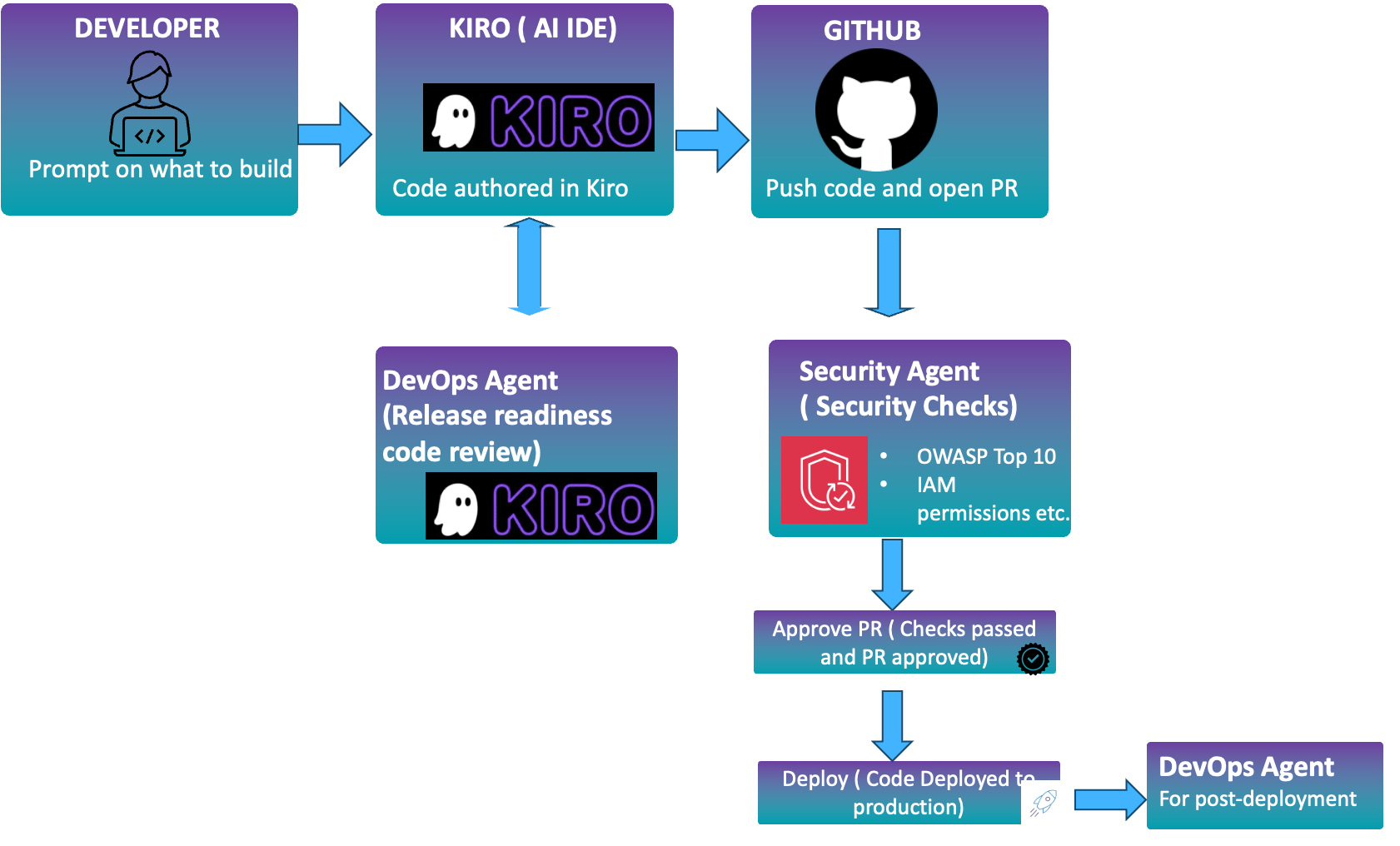
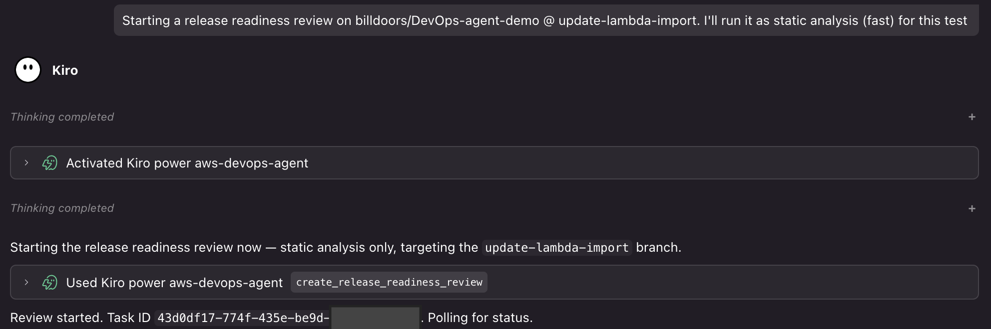
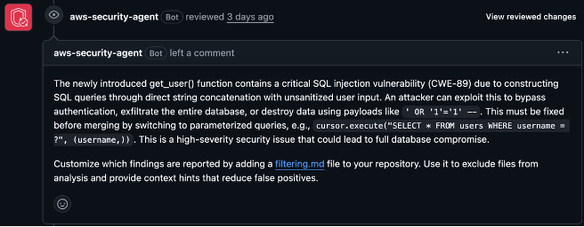
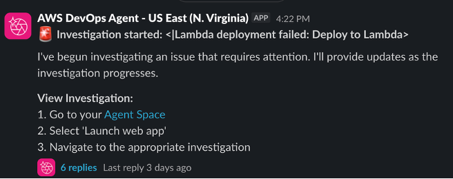
Zellij is a relatively new entrant in the terminal-multiplexer
category. Like GNU
Screen and tmux it gives
users the ability to manage a workspace inside a terminal with split panes,
provides session management, and so forth; but Zellij also includes a web server for
browser access to a terminal session, is extensible via a plugin API, and is likely
more beginner-friendly than its predecessors. Its most recent release, version 0.46,
adds a standalone terminal emulator, a built-in inbox for notifications, and a settings
screen so users can configure the application without fussing with
configuration files. While the low version number might suggest that it is not
yet ready for serious use, it seems stable and full-featured enough to
meet the needs of many users.
Approving an AI service is only the starting point. As employees adopt Claude and their responsibilities change, security teams need to know who has access, which users hold administrative privileges, and whether those roles and group memberships still reflect the work they do.
IBM’s 2025 Cost of a Data Breach Report found that, among studied organizations reporting an AI-related breach, 97% lacked proper AI access controls. The finding highlights a broader challenge: AI adoption needs security practices that extend beyond the initial approval, supported by information teams can use to review access with administrators and service owners.
Rapid7 Surface Command now integrates with Claude’s Compliance API, bringing supported organization, user, role, group, and settings information into the same platform teams use to understand other assets and identities. The integration helps security teams make enterprise Claude access part of their existing review practices.
Bring enterprise AI access into your security view
An account list tells security teams who is present, while roles and group memberships help explain how access is organized and where further review may be needed. Surface Command’s integration with Claude’s Compliance API brings together:
Organizations and users: Visibility into the Claude organization and its associated user accounts.
Roles and groups: Context to understand users’ assigned roles and group memberships.
Organizational settings: Available configuration information to support review of the enterprise Claude environment.
With those details in Surface Command, practitioners can examine Claude identities alongside the other assets and identities they manage. That gives them a clearer basis for working with service owners to evaluate whether access remains appropriate as teams and responsibilities change.
The integration focuses on administrative visibility. It does not ingest Claude conversation content, provide threat detection on Claude activity, or control Claude’s behavior.
From a user record to an informed access review
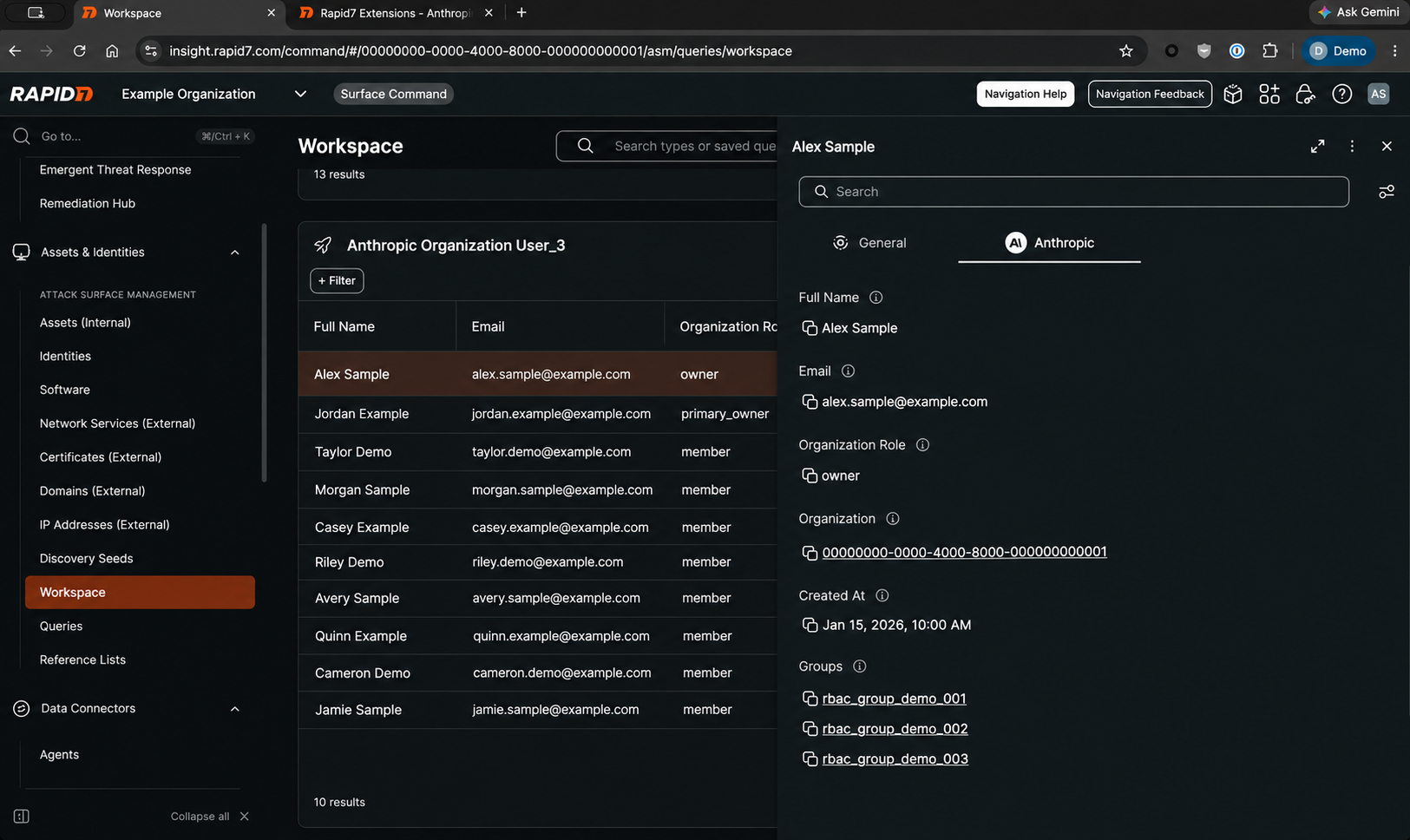
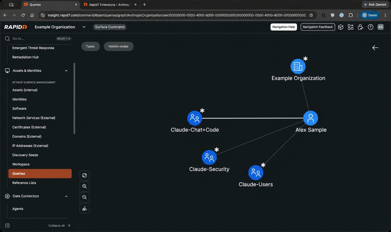
Consider a security practitioner reviewing administrative access to Claude. In Surface Command, they can inspect an imported user’s details, review their organization role and administrative status, and examine their group memberships. The relationship graph provides a visual view of how that user connects to the organization and its groups, making those associations easier to follow.
The practitioner can then work with the service owner to confirm whether administrative privileges are still needed, whether group memberships reflect current responsibilities, and whether those assignments align with the organization’s access model.
Surface Command provides information to support the review, while the team applies its policies and judgment to determine whether a change is needed.
Support AI adoption with clearer accountability
As Claude becomes part of everyday work, reviewing its users and access relationships becomes part of managing the environment. Bringing that information into Surface Command helps security practitioners and service owners work from a shared understanding of assigned roles and group memberships. It supports more informed access decisions and helps security leaders incorporate enterprise AI into established oversight practices.
Get started with Claude and Surface Command today
The integration is available through the Anthropic connector in the Rapid7 Extension Library. Using Claude’s Compliance API requires a Compliance API key and the appropriate entitlement for your Claude organization.
Visit the connector page to get started and see how Surface Command brings Claude users, roles, and group relationships into view.
Google Deepmind researchers used agentic AI to mathematically prove, or “formally verify,” a number of the Signal protocol’s key cryptographic guaranteesa landmark development for the widely used cryptography and AI itself.
Conducted as a sort of proof-of-concept project in just four weeks, the work is significant in two ways. It serves as further independent validation of the cryptography that protects massive quantities of the world’s communications on platforms like the Signal app, Google Messages, and WhatsApp. And it demonstrates Google DeepMind’s formal verification capabilities using a new AI framework called AlphaProof Code.
[…]
The DeepMind analysis did not find any new vulnerabilities in the portions of the Signal protocol it looked at, but when the researchers used AlphaProof Code on older versions of Signal that contain known and long-fixed vulnerabilities, it correctly identified them and showed that the protocol could not be formally verified. The researchers are releasing the specification and proof they developed for the Signal protocol analysis to aid other formal verification work.
First, our researchers collaborated with a mix of models to translate Signal’s security goals into formal mathematical specifications, with human experts reviewing every one. From there, agents powered by Gemini Carbon did the proofs, generating over six million lines of Lean, a computer language that mathematically proves the accuracy of code.
Next, the agents audited the proof and highlighted areas that needed a second look by a human just one percent of the codebase, a massive time savings. Because Lean automatically checks the rest, our experts could focus their review where human judgment matters most.
Amazon Managed Streaming for Apache Kafka (Amazon MSK) Express brokers deliver Apache Kafka topic data to general purpose Amazon Simple Storage Service (Amazon S3) buckets at lower cost and without the operational overhead of running Kafka Connect. Because Express brokers handle both ingestion and delivery, you can reduce your ingestion and delivery costs by up to 60% compared to self-managed alternatives. There is no connector or infrastructure to manage, you pay only for the data delivered, and delivery doesn’t consume broker throughput.
Many Kafka workloads need a durable copy at rest in Amazon S3 for backup and archive. Compliance rules often require you to keep raw events for years for audits. You require a replayable copy that outlives topic retention, raw training data for artificial intelligence and machine learning (AI/ML) models, and a staging area for scheduled extract, transform, and load (ETL) jobs. For analytics, Express brokers also deliver to streaming tables, which continuously materialize your Kafka topics as Apache Iceberg tables on Amazon S3 Tables, a capability of Amazon S3, with no Kafka connectors, Apache Flink jobs, or custom consumers to run. The tables are registered automatically in AWS Glue Data Catalog, so you can query them with Amazon Athena, Amazon Redshift, and Apache Spark, and inline compaction reduces downstream query costs by up to 30%. Because delivery doesn’t add broker load, one topic can feed both an S3 bucket and a streaming table. For more information, see Deliver Apache Kafka data to streaming tables for Apache Iceberg with Amazon MSK Express brokers.
In this post, we look at the two challenges of delivering Kafka data to Amazon S3 today, managing Kafka brokers and managing the delivery pipeline, and how Express brokers and data delivery to Amazon S3 address each one. We then walk through the architecture and show how to get started on the console and with Agent Skills.
Challenges with delivering streaming data to Amazon S3 on self-managed Kafka
To deliver Kafka data to Amazon S3 today, you typically run an S3 sink connector on Kafka Connect next to your Kafka cluster. That leaves you with two systems to run:
Managing Kafka brokers: You size and provision broker storage upfront, monitor its utilization to avoid disruptions, and keep paying for it even if your workload scales down. You recover failed brokers, manage Kafka configurations for availability and performance, and patch brokers during maintenance windows. Adding capacity means provisioning brokers and rebalancing partitions, which can take hours or days, so you size the cluster for peak traffic and plan scaling well ahead.
Managing the delivery pipeline: Running Kafka Connect typically causes the following three challenges:
Operational complexity: You find or build a connector, take it through security approval, deploy it, and apply security updates across your Kafka Connect workers. When delivery fails, you troubleshoot across brokers, workers, and Amazon S3.
Cost: You size Kafka Connect workers for peak demand and keep paying for it when traffic is low, and a pipeline assembled from several services adds a charge at every hop.
Contention with real-time consumers: A connector reading from a Kafka topic consumes broker egress throughput, so feeding the archive competes with your real-time applications. Cluster scaling and version upgrades can also interrupt delivery.
How Express brokers and data delivery to Amazon S3 address these challenges
Managing Kafka brokers: Express brokers include pay-as-you-go storage that scales automatically, so there’s no storage to size, provision, or monitor. When your workload scales down, the cluster uses less storage and your storage charges go down automatically. MSK recovers failed brokers for you, manages critical cluster and topic configurations for availability and performance on your behalf, and updates cluster hardware on an ongoing basis with no maintenance windows. To add capacity, you add brokers, and Express rebalances partitions onto them in minutes, so you don’t need to over-provision for traffic spikes or plan scaling far ahead. For details, see Simplifying Kafka operations with Amazon MSK Express brokers. To move from self-managed or third-party Kafka, Amazon MSK Replicator copies your data and consumer group offsets into an Express cluster, and the migrate-to-msk Agent Skill recommends a right-sized Express cluster before you start. For more information, see Migrate Kafka workloads to an Amazon MSK cluster.
Managing the delivery pipeline: Data delivery to Amazon S3 is built into Express brokers, so there’s no Kafka Connect to run. You create a channel on a topic, and MSK runs the delivery. This addresses each of the three challenges:
Operational complexity: There’s no connector to find, build, or take through security approval, nothing to deploy beyond the channel, and no workers to patch. MSK handles retries and backpressure. When a record can’t be processed, the channel writes its identifiers and error context to a dead-letter queue (DLQ) bucket and delivery continues, and you troubleshoot in one place, through the channel’s Amazon CloudWatch metrics and logs.
Cost: There’s no capacity to size for peak, because MSK scales delivery with your workload. You pay only for the data delivered, billed per byte, so you pay less when traffic is low. Delivery adds one charge on top of standard Amazon S3 charges, with no connector or worker fees, no charge for the broker egress that delivery uses, and no charge for records routed to the DLQ.
Contention with real-time consumers: The channel reads the topic without consuming broker throughput, so archiving doesn’t compete with your real-time applications, and you can add channels to a topic without adding broker load. Capacity scaling and version upgrades happen without delivery gaps.
MSK data delivery to Amazon S3 architecture
Producers write to a Kafka topic exactly as they do today. The channel reads records from the topic, batches them, and writes them as objects to your S3 bucket. You choose the compression (NONE, GZIP, or ZSTD), the storage class (S3 Standard, S3 Intelligent-Tiering, or S3 Glacier Instant Retrieval), and an output key template that defines the object key layout, such as date-based prefixes with the partition and offset in each object name. Records keep the format the producer wrote them in, whether JSON, UTF-8 strings, or raw bytes, and no schema registry is required.
For JSON and String records, the channel validates each record. If a record fails validation, the channel writes the record’s identifiers and the error context to the DLQ bucket in Amazon S3, and delivery continues. You can also send delivery logs to Amazon CloudWatch Logs, Amazon S3, or Amazon Data Firehose.
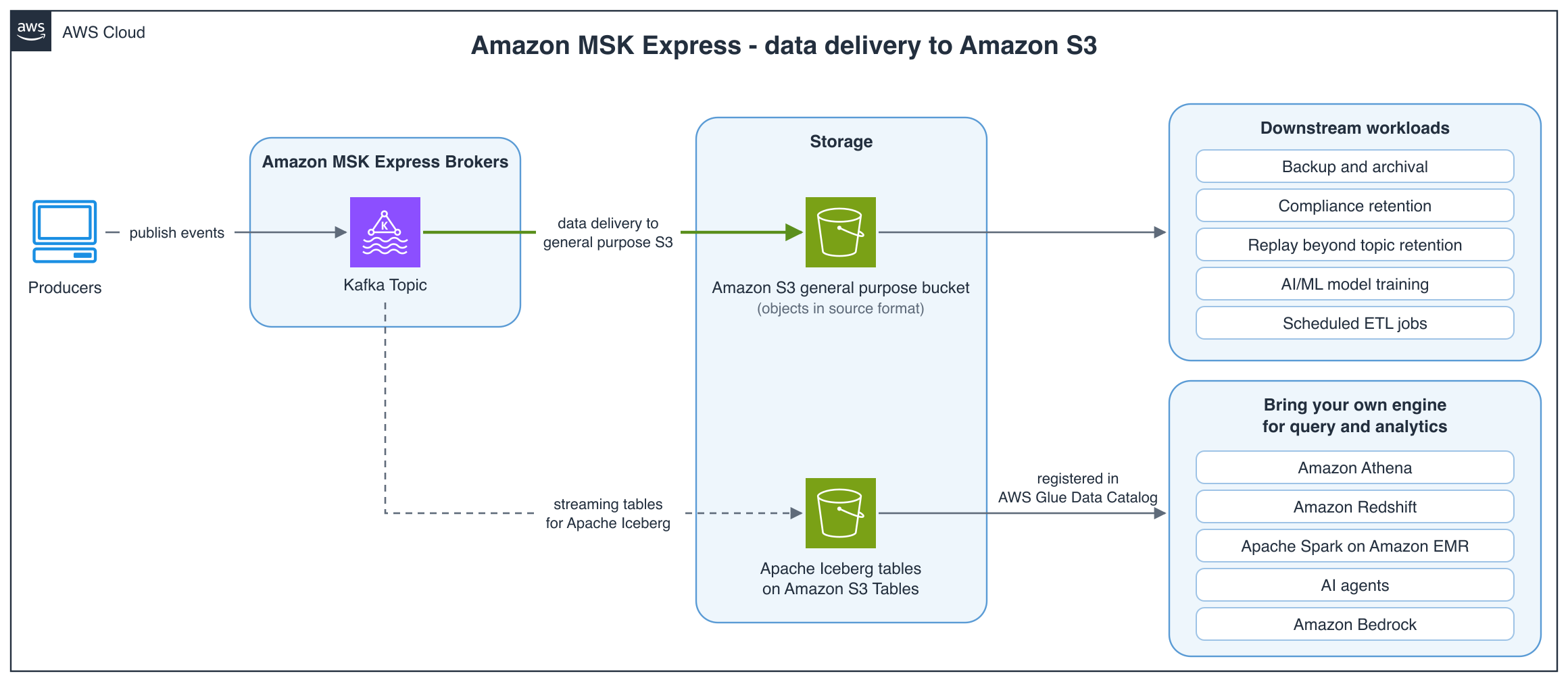
The following diagram illustrates this architecture.
Figure 1: Producers publish to a Kafka topic on Amazon MSK Express brokers. Data delivery writes the topic to a general purpose S3 bucket as objects in their source format, which you can use for backup and archival, compliance retention, replay beyond topic retention, AI/ML model training, and scheduled ETL jobs. Streaming tables write the same topic to Apache Iceberg tables on Amazon S3 Tables, registered in AWS Glue Data Catalog, so you can bring your own engine for query and analytics, such as Amazon Athena, Amazon Redshift, Apache Spark on Amazon EMR, or AI agents built with Amazon Bedrock. No connector runs between the cluster and Amazon S3
If you’re moving from an existing connector, create the channel before you retire the connector, and keep both running until you confirm that the delivered data overlaps.
You can also manage channels with the Amazon MSK APIs and the AWS Command Line Interface (AWS CLI) (for example, aws kafka create-channel) through infrastructure as code or automation across many clusters and topics, or let an AI agent do it for you, as the next section shows.
Getting started with Agent Skills
AWS publishes open source Agent Skills, available through the Agent Toolkit for AWS, that give AI coding agents guidance for configuring delivery on services. The managing-amazon-msk skill covers data delivery to Amazon S3 on an Express broker cluster. The skills guide your agent through the setup steps that are easy to get wrong: the IAM role and trust policy, output key template rules, DLQ setup, and verifying delivery after the channel is running.
Skills are discovered automatically by compatible tools through the SKILL.md file. Follow the Agent Toolkit installation guide, then add the skill for the service you are working with:
We also recommend installing the AWS MCP Server, which gives your agent tools for searching AWS documentation, blogs, and Skills dynamically at runtime. This makes both discovery and installation more flexible, and the agent itself more accurate. To verify the installation, interact with the skill in your preferred tool.
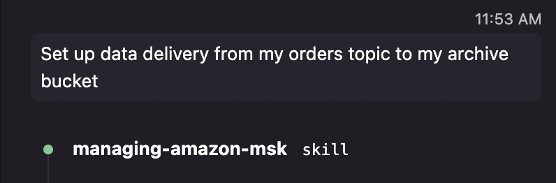
To begin delivery, prompt your agent of choice. For Amazon MSK, “Set up data delivery from my orders topic to my archive bucket”:
Figure 2: Issuing the delivery prompt in an agent chat
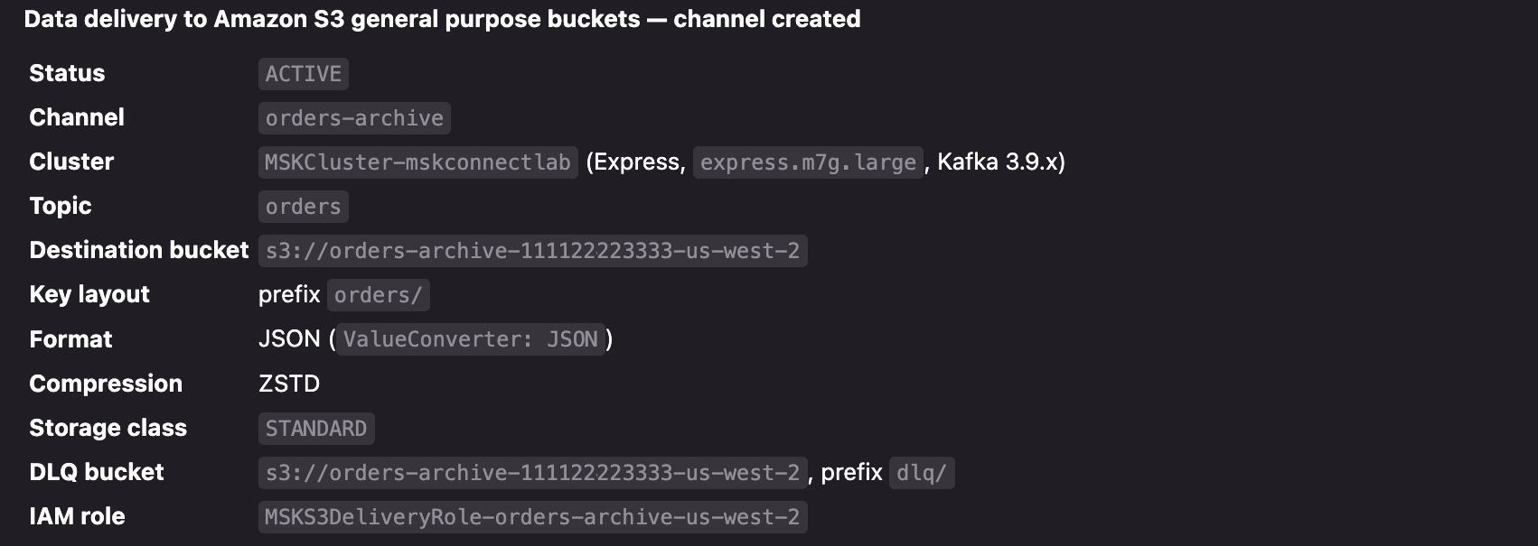
The agent first dynamically loads the relevant skill, inventories the clusters, topics, and buckets available in your account. It then confirms the resources to use or create before creating the delivery configuration. After creation, the agent summarizes the status and can help with the data operations that follow, such as setting up an AWS Glue crawler so the delivered objects are queryable as partitioned tables in Amazon Athena, or configuring CloudWatch alarms on delivery freshness and dead-letter queue activity.
Figure 3: The agent creates the channel
Clean up
To avoid ongoing charges, delete the resources you created for this walkthrough. An active channel keeps delivering records and incurring delivery charges until you delete it. On Amazon MSK, open your cluster in the Amazon MSK console, choose the Channel tab, and delete the channel. Objects already written to Amazon S3 keep incurring storage charges after the channel is deleted, so delete the delivered objects, and the destination and DLQ buckets if you no longer need them. Finally, delete the IAM service execution role and any CloudWatch log groups created for the channel, including any that your agent created.
Conclusion
With data delivery to Amazon S3 on Amazon MSK, you can keep a durable copy of your streaming data in Amazon S3 without running a connector. You pay only for data that is delivered, and delivery doesn’t compete with your real-time consumers for throughput.
At British Airways (BA), engineering at scale means supporting services used across the airline for millions of passengers, while simultaneously preparing for what comes next. After completing a major migration of legacy data center infrastructure to AWS, the next question was how BA could use its new cloud capabilities to improve scalability and efficiency. The team also wanted to accelerate the next phase of modernization.
As part of this next phase, BA began exploring how agentic AI could help accelerate the modernization of its technology estate. Working with AWS, the team identified AWS Transform custom as a way to support this at scale. This purpose-built solution is designed to modernize large legacy platforms using agentic AI and automation. The first major target was a legacy Java platform of more than 250 business services across around 750 code repositories. BA set out to migrate it from Amazon Elastic Compute Cloud (Amazon EC2) to a modern, cloud-native architecture on Amazon Elastic Container Service (Amazon ECS) with AWS Fargate and AWS Graviton. The new architecture is containerized, auto scaling, and resilient by design.
About British Airways
British Airways is the UK’s flag carrier airline, serving more than 40 million customers annually across more than 200 destinations worldwide, and a subsidiary of International Airlines Group (IAG).
Challenge
British Airways’ Java platform had supported the airline for many years, but maintaining and updating it required valuable engineering time that could be more efficiently spent advancing innovation. As BA continued to modernize its technology foundations, the team identified an opportunity to move services to a more scalable architecture and simplify their ongoing management.
“Can AI really transform hundreds of code repositories at enterprise scale? That was the question everyone asked when we started this journey. With more than 250 business services on a legacy platform, maintaining the estate demanded considerable engineering time. We needed a more efficient approach that would free our teams to focus on innovation rather than routine maintenance.”
— Gary Holland, Principal Platform Architect at British Airways
Solution
British Airways partnered with AWS to deploy AWS Transform custom, purpose-built to modernize large legacy estates using agentic AI and automation. Starting with an Experience Based Acceleration (EBA) using Amazon Q Developer, the team moved swiftly. When AWS Transform custom launched at AWS re:Invent 2025, BA was among the first to build with it. Its first fully transformed service went live in production shortly after.
How the transformation engine works
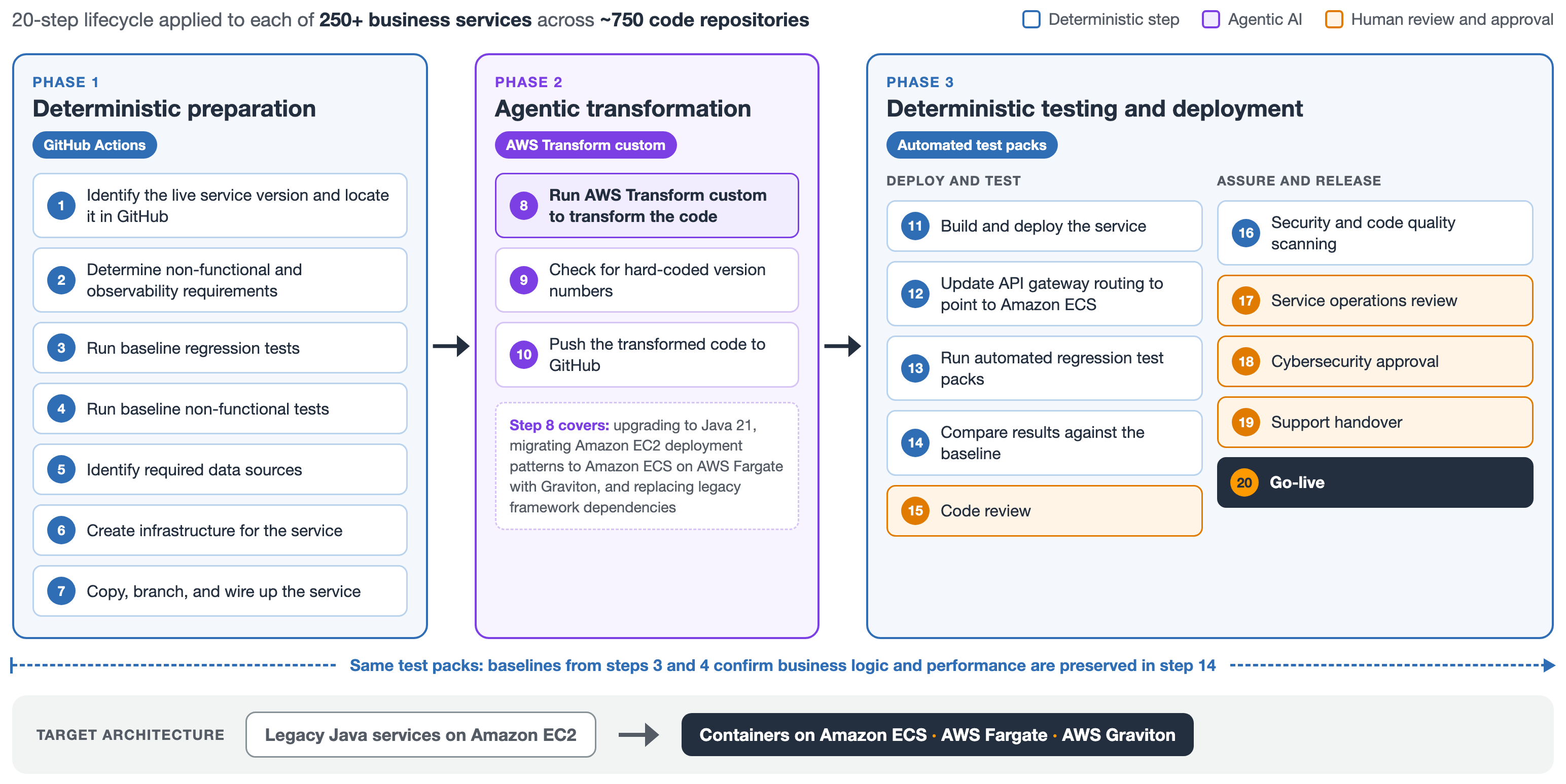
Each service passes through a 20-step transformation lifecycle that blends deterministic automation with agentic AI, designed to be repeatable across hundreds of services without manual re-engineering.
Figure 1: The 20-step transformation lifecycle British Airways uses with AWS Transform custom
Phase 1: Deterministic preparation. GitHub Actions workflows analyze each service repository to identify the production-versioned artifact currently deployed, then catalog its dependencies and data source configurations. Automation runs against live production logs to extract peak and mean traffic rates. It then infers the non-functional requirements (scaling thresholds, resource sizing, and observability settings) needed to configure each service’s new container on Amazon ECS. Baseline regression and performance test packs are executed against the existing platform to establish a known-good benchmark before any code is touched. The infrastructure for each service is then created, and the service code is copied, branched, and wired up, ready for transformation.
Phase 2: Agentic transformation. AWS Transform custom transforms the codebase for the target architecture. This includes upgrading to Java 21 and migrating from Amazon EC2 deployment patterns to Amazon ECS on AWS Fargate with Graviton. It also replaces legacy framework dependencies and resolves hard-coded version numbers that would otherwise block future patching. The agentic engine handles the complex transformation activity that would previously have consumed months of engineering time per service. The team then checks for any remaining hard-coded version numbers and pushes the transformed code to GitHub.
Phase 3: Deterministic testing and deployment. The transformed code is built and deployed into lower environments, and API gateway routing is updated to point to Amazon ECS. The service is then validated through the same automated regression and performance test packs run during Phase 1. Results are compared against the baseline to confirm that business logic is preserved. Human-in-the-loop code reviews, security and code quality scanning, a service operations review, and cybersecurity approval confirm that every service meets BA’s standards before support handover and go-live.
This separation of concerns is deliberate. Deterministic steps handle everything that should be repeatable and auditable. Agentic AI handles the complex transformation work that would otherwise consume months of engineering time. The result is a repeatable engine that can securely and accurately process hundreds of services far faster than a manual, service-by-service migration.
With AWS Transform custom, British Airways can:
Accelerate the modernization of Java services while reducing the manual effort required from engineers.
Move services from Amazon EC2 to a more scalable architecture using Amazon ECS on AWS Fargate with Graviton, supported by testing and assurance to confirm that business logic continues to perform as intended.
Upgrade outdated software versions and frameworks, supporting a more resilient and maintainable platform.
Apply lessons from the work to other engineering activities, including improving unit-test coverage.
Outcome
The benefits go beyond the technology itself. By reducing the manual effort involved in modernization, BA can give engineers more time to focus on resilient technology and better experiences for colleagues and customers.
“Modernising hundreds of code repositories is a significant engineering challenge. By combining agentic and generative AI and automation with human review and assurance, we’re accelerating that work and reducing the manual effort involved. Most importantly, it gives our engineers more time to focus on delivering value to the business and better experiences for our colleagues and customers.”
— Gary Holland, Principal Platform Architect at British Airways
“This is more than a technology upgrade. It is about building stronger, more resilient technology foundations for British Airways so our teams can deliver change more quickly and create better experiences for our customers. The early results are encouraging, and we are now applying what we have learned across the wider platform.”
— Liz Wright, Director of Delivery for BA Digital Customer and Commercial
Get started today
For British Airways, the work demonstrates how modern cloud technology, automation, and responsible use of AI can strengthen the airline’s technology foundations and create more capacity to innovate for customers.
If you’re planning to modernize your own Java applications, explore AWS Transform custom to see how agentic AI and automation, combined with human review, can reduce the manual effort involved.
If you have run Apache Solr for years, you can offload its undifferentiated operational overhead: managing ZooKeeper quorums, patching JVMs, tuning garbage collection, and building custom plugins for features a managed service provides out of the box. Moving to a managed service with native AWS integrations and capabilities like vector search is attractive, but the migration itself is what keeps you on aging infrastructure. Schemas differ between Solr and OpenSearch. Application code is written against the Solr HTTP API, custom analyzers are baked in, and the project balloons into months of engineering work.
A 2024 AWS Big Data Blog post on migrating from Apache Solr to OpenSearch laid out the conceptual differences between the two engines and what to think about at a planning level. However, it left the execution to the reader. In this post, you execute a Solr-to-OpenSearch Serverless migration end to end using the Migration Assistant for Amazon OpenSearch Service from the AWS Solutions Library that runs on Amazon Elastic Kubernetes Service (Amazon EKS). It orchestrates the migration. The Migration Assistant Command Line Interface (CLI) includes a built-in interactive mode that guides you through the assessment and execution in plain language. If you’re only assessing a migration, you can run the AI advisor standalone from your development environment without provisioning infrastructure.
This walkthrough uses Apache Solr 9.6 as the source with a demo catalog of 600,000 synthetic product documents. The same flow applies if you are running Elasticsearch 5.x or later, or a self-managed OpenSearch cluster as your source.
Note: The prompts and responses shown in this post are directional. Because interactive mode uses natural language, your exact prompts and responses might vary by Migration Assistant version and your environment.
By the end of this post, you will have migrated a 600,000-document Apache Solr catalog to Amazon OpenSearch Serverless using the AI-driven agent mode in the Migration Assistant for Amazon OpenSearch Service, from assessment through validated backfill. On the target, you no longer maintain ZooKeeper quorums, JVMs, or custom plugins.
Solution overview
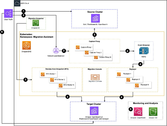
The Migration Assistant for Amazon OpenSearch Service guides you through the various phases of the migration, including deploying the necessary infrastructure components, such as an Amazon EKS cluster. The Migration Assistant guides you through three phases:
Assess – Inventory the source schema and query patterns. Check permissions and accessibility. Surface incompatibilities before any data moves.
Backfill – Snapshot the source into Amazon Simple Storage Service (Amazon S3), then stream the snapshot into the target using Reindex-from-Snapshot (RFS).
Validate – Compare document counts, mappings, sample query results, and replay consistency between source and target.
Figure 1: Migration Assistant architecture on Amazon EKS, showing the RFS workers for backfill and the capture proxies for live traffic
Prerequisites
Before starting, verify that you have the following:
A compatible coding assistant installed and configured. Agent Mode runs inside supported development environments.
AWS credentials configured for the target account (AWS IAM Identity Center, temporary credentials, or an AWS Identity and Access Management (IAM) role with sufficient permissions).
Account isolation – Use a dedicated non-production account for this walkthrough, or assume a scoped deployment role with short-lived credentials from AWS IAM Identity Center. Point the Migration Assistant at a non-production Solr, Elasticsearch, or OpenSearch source.
Deployment permissions – The deployment creates a VPC, a NAT gateway, an Amazon EKS cluster, IAM roles, an Amazon Elastic Container Registry (Amazon ECR) repository, and an Amazon S3 bucket through AWS CloudFormation, so the deploying principal needs permissions to create those resources and to pass roles (iam:PassRole). See the Migration Assistant required-permissions guidance for the exact policy.
Workflow pod scope – The migration workflow pods use Amazon EKS Pod Identity to assume a role limited to the snapshot and capture Amazon S3 bucket and the target OpenSearch Serverless collection, rather than broad account access.
AWS Command Line Interface (AWS CLI) v2 (latest 2.x release recommended) installed and configured.
Verify installation: aws --version.
kubectl and Helm installed (the agent uses kubectl to interact with the Amazon EKS-based Migration Assistant infrastructure, and the deployment installs the Migration Assistant as a Helm chart).
Confirm both are on your PATH: kubectl version --client && helm version.
Network access from your workstation to AWS APIs and, optionally, to the source cluster for assessment.
Source cluster details – Endpoint, version, and authentication method for your Solr, Elasticsearch, or OpenSearch cluster.
The tool will prompt you if any of the above aren’t configured.
The install script comes from the official AWS Solutions release channel, the solutions-reference Amazon S3 bucket, and is published by the AWS Solutions release pipeline. For transparency, you can review the source for Migration Assistant for Amazon OpenSearch Service in the aws-solutions/migration-assistant-for-amazon-opensearch repository on GitHub. This post pins version 3.98.7 for repeatable results. Check the Migration Assistant documentation for the current release and substitute the latest version in the install URL.
The one-line command pipes a script straight into bash. The 3.98.7 script runs without sudo. It downloads a single platform binary into ~/.local/bin and runs chmod +x on it, but it doesn’t verify a checksum or signature, and checksums are not currently published for the binaries. The only protection is HTTPS from the AWS-owned Amazon S3 bucket. For a safer install, download the script first, review it, then run it:
curl -fsSL https://solutions-reference.s3.us-east-1.amazonaws.com/migration-assistant-for-amazon-opensearch-service/3.98.7/install.sh -o install.sh
less install.sh # review what the script does before running it
bash install.sh
The installer places the migration-assistant binary on your PATH and prompts you to launch the Migration Assistant by running the following:
migration-assistant
You’re given two options: Manual or Agent Mode. Choose Agent Mode for an AI-guided migration experience.
If you have more than one supported development assistant on your PATH, the CLI detects them and asks which one to use.
Select your preferred option to proceed with the migration.
The interactive mode then prompts you for what you want to accomplish. You can request:
An assessment – The agent connects to your source cluster (read-only), analyzes the schema, identifies compatibility gaps, and produces a migration assessment report.
A deployment – The agent deploys the Migration Assistant infrastructure (an AWS CloudFormation stack, Amazon EKS cluster, and Helm chart) into your AWS account.
A migration – The agent configures and runs the end-to-end migration workflow, including historical data backfill and optional live traffic capture and replay.
Describe your goal in plain language. For example, “Assess my Solr 9.6 cluster. I am evaluating a migration” or “Migrate my Solr 8.11 cluster to OpenSearch Serverless.”
Data handling in agent mode – Agent mode runs inside a third-party coding assistant. To reason about your migration, the agent sends context to that model, including your Solr schema and solrconfig.xml, sample queries, and your source and target endpoints. If you have data-handling rules, review what your coding assistant transmits before you use agent mode.
The agent doesn’t store your credentials and shows each command before it runs. The local ./migration-assistant-workspace/ folder holds migration state, logs, and the assessment report, so treat that folder as sensitive and protect it like other credential-adjacent artifacts.
Assessing a migration
The first step is to run a full assessment of the source cluster. In this phase, nothing changes on the source. The agent takes inventory and reports back on what is missing or incompatible. Tell Migration Assistant to perform the assessment:
“Run a migration assessment of my Solr collection. The source is Solr 9.6.1 in SolrCloud mode at https://solr.example.internal:8983/solr, collection name products, 600,000 docs.”
You provide the source location directly in the prompt. Give the agent the Solr endpoint (for SolrCloud, any node’s base URL, or your ZooKeeper connection string) along with the collection name and authentication method. If you leave out the endpoint, the agent asks for it before it connects, because the assessment phase needs to reach the source to read the schema and solrconfig.xml.
The agent connects to Solr in read-only mode, takes inventory of the collection, and prints a structured report covering:
Networking – Verifies Migration Assistant can reach the source and that the S3 snapshot repository is loaded in Solr.
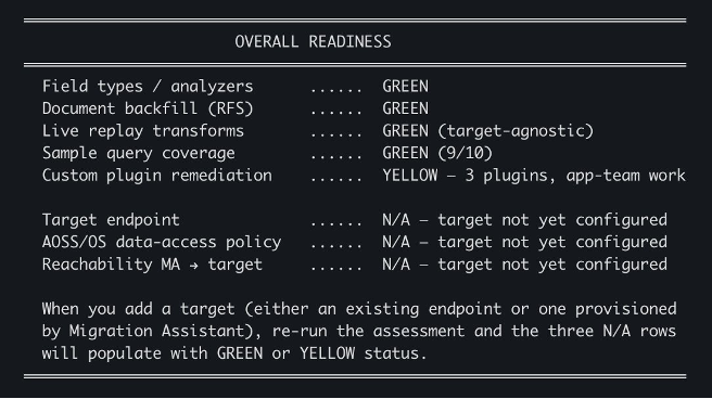
The following screenshot shows the bottom of the assessment report, which details overall readiness based on what the agent found after examining source and target configurations.
Figure 2: Overall readiness section of the assessment report, where source-side checks pass green and custom plugin remediation is yellow
Field types, document backfill (RFS), live replay transforms, and sample query coverage all pass green. Custom plugin remediation is listed as yellow because the assessment detected three custom Java plugins in the solrconfig.xml that don’t translate automatically and require refactoring by your team. The target-side checks show N/A because a target has not been configured yet. After you add a target endpoint, re-running the assessment populates those rows.
Deploying the Migration Assistant infrastructure
Before moving on, save the assessment report so the findings stay available as a reference during the migration. The agent stores the report in your workspace and can recall specific findings later when you configure the workflow.
A green assessment report indicates that migration is possible and does not move the data. Migration Assistant will be used to migrate the data and build necessary configurations. The Migration Assistant needs infrastructure deployed in your account before it can copy data from Solr to Amazon OpenSearch Serverless. Ask the agent to deploy that infrastructure:
“Deploy the Migration Assistant infrastructure in us-west-2”
When you start the deployment, the agent asks for a stage name. The stage is a label you choose, not a value from a fixed list. The agent uses it as the Kubernetes namespace for the pods, the Helm release name, and the suffix on the CloudFormation stack (MigrationAssistant-<stage>). Accept the default ma, or pick something more descriptive like dev, prod, or solr-migration.
Under the hood, the agent deploys a CloudFormation stack that provisions:
An Amazon S3 bucket for snapshot storage and captured traffic tuples.
Total time to install the Migration Assistant is approximately 10–15 minutes. The agent monitors pod state and reports when the infrastructure is ready.
Backfilling Solr data
After addressing data-access gaps and confirming the assessment is green, you instruct the agent to run the backfill and give it the target endpoint:
“Run the backfill into my OpenSearch Serverless collection at”
You specify the target OpenSearch Serverless endpoint here, in the backfill request. If you leave it out, the agent asks for the collection endpoint and confirms the Region and SigV4 authentication before it builds the workflow. You review that configuration next.
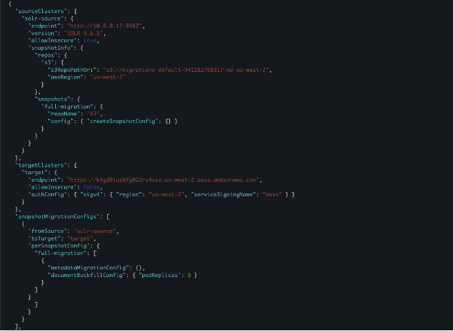
Before starting the backfill, the agent generates a workflow configuration that captures the migration configuration in a single JSON document: source and target endpoints, authentication, snapshot location, and RFS worker settings. The agent prints the configuration for you to review and approve, so nothing runs until you confirm.
Figure 3: Workflow configuration JSON, part 1, showing the source cluster, S3 snapshot repository, target OpenSearch Serverless endpoint, and RFS worker settings
The JSON defines the source Solr cluster endpoint and version, the S3 bucket where the Solr snapshot is stored, and the target OpenSearch Serverless collection endpoint. Because the Migration Assistant uses Reindex-from-Snapshot, you point the s3RepoPathUri at the S3 bucket provided for storing the snapshot. The target can be either an Amazon OpenSearch Service domain or an OpenSearch Serverless collection.
This Solr cluster uses basic authentication. You can create a Kubernetes secret in the Migration Assistant namespace after deployment and reference that secret by name in the workflow configuration. You can ask the agent to create the secret, or run the command yourself:
kubectl create secret generic solr-basic-auth --namespace ma --from-literal=username='YOUR_SOLR_USERNAME' --from-literal=password='YOUR_SOLR_PASSWORD'
The preceding command passes the password with --from-literal, which leaves it in your shell history and the process list. For anything beyond a quick test, read the password without echoing it and pass it through a restricted-permission file that you delete afterward:
read -s SOLR_PASSWORD # prompt without echoing to the terminal
umask 077 # restrict permissions on files you create
printf '%s' "$SOLR_PASSWORD" > solr-password.txt
kubectl create secret generic solr-basic-auth --namespace ma \
--from-literal=username='YOUR_SOLR_USERNAME' \
--from-file=password=solr-password.txt
rm -f solr-password.txt # remove the file once the secret exists
unset SOLR_PASSWORD
As an alternative, store the Solr credential in AWS Secrets Manager and resolve it at deploy time instead of placing it in a shell command. Either approach keeps the password out of your shell history and the process list.
Use the stage name you chose during deployment as the namespace (ma is the default), and reference the secret name (solr-basic-auth) in the workflow configuration so the agent can authenticate the source.
Grant the target collection a data access policy
For an OpenSearch Serverless target, the Migration Assistant workflow pod role must be allowed to write to the target collection. Grant that access through a data access policy scoped to the target collection and index, and confirm the collection is reachable through its network policy. Scope the policy to the specific collection and index rather than *:
Reindex-from-Snapshot reads a Solr snapshot from Amazon S3, so the Solr nodes need write access to the snapshot bucket to create that snapshot. Attach an IAM policy scoped to only the snapshot bucket and prefix rather than a broad Amazon S3 grant:
Turn on Amazon S3 Block Public Access for the bucket and turn on encryption at rest, either with Amazon S3 managed keys (SSE-S3) or AWS Key Management Service (AWS KMS) keys (SSE-KMS).
The same bucket also holds captured traffic tuples, which can contain real user queries and personally identifiable information (PII). Keep that data only as long as you need it for cutover validation, and delete it after cutover.
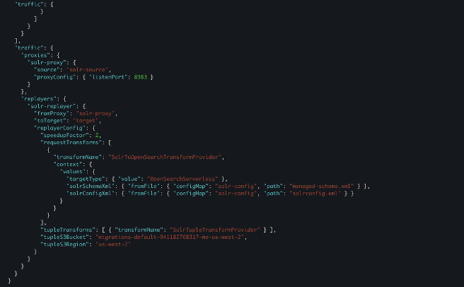
To capture live traffic updates as part of the migration, the configuration also provides a replayer. The replayer captures live traffic at the source through a proxy and mirrors it into the target. The Migration Assistant uses SolrToOpenSearchTransformProvider to read the Solr schema and config files to translate queries in real time.
Figure 4: Workflow configuration JSON, part 2, showing the capture proxy and the replayer with the SolrToOpenSearchTransformProvider for live query translation
After you approve the workflow, the Migration Assistant control plane starts spinning up resources. Within about a minute, the migration-console pod reports that the metadata phase ran successfully and can create an index in the target collection.
If the tool can’t migrate a specific item, the tool logs the issue and continues where safe. Some issues are fatal, such as an index that already exists on the target or a field type the transformer can’t convert. These cause the phase to exit non-zero so you can fix the problem and rerun. The Migration Assistant skips already migrated items on retry.
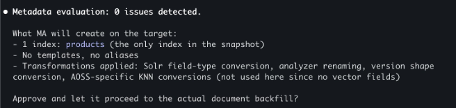
Some categories are out of scope for the metadata phase and require separate planning: security configuration, ISM and ILM policies, ingest pipelines, Dashboards saved objects, data streams, and cluster level settings.
Figure 5: Metadata evaluation output showing zero issues detected and one index, products, to create on the target
Open a second terminal to monitor the migration. Launch migration-assistant and select [1] Manual when asked how you want to drive the migration, which opens the migration-console. With the migration-console open, run the following command to confirm the target index was created with zero documents:
console clusters cat-indices --cluster target
Figure 6: cat-indices output showing the products index created with 0 documents, confirming the metadata migration succeeded
The agent confirms the mappings are correct, including the dynamic templates for Solr’s dynamic-field patterns, and asks for approval to start RFS. You approve, and RFS workers spin up on EKS. To watch documents flow into the target in real time, run a watch loop against the same cat-indices command in the migration-console:
The console command inside the migration console pod exposes utilities for driving and inspecting a migration outside the workflow CLI. In addition to clusters cat-indices, you have clusters connection-check, clusters curl, and snapshot, among others. Run console --help inside the pod to view the full list.
The document count climbs steadily as the three RFS worker pods stream the snapshot into the new index. The workflow configuration you approved earlier set three RFS worker replicas, so three pods run the backfill in parallel here. You can raise or lower that replica count to control how much the backfill parallelizes. The following screenshot shows the migration mid-flight at roughly the halfway point.
Figure 7: Mid-flight progress showing 304,441 documents migrated into the products index
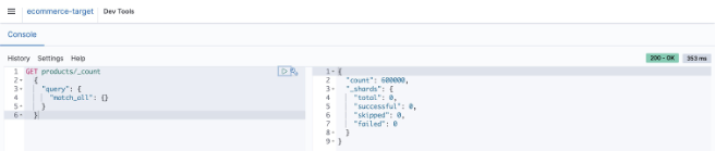
After the backfill completes, you can confirm the final document count directly from OpenSearch Dashboards Dev Tools. The following query against the migrated collection returns the exact count:
OpenSearch Dashboards Dev Tools showing a document count query returning 600,000 documents
*Figure 8: OpenSearch Dashboards Dev Tools, where GET products/_count returns 600,000 documents, confirming the backfill is complete*
Validation and testing
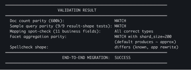
With the backfill finished, ask the agent to run a validation check. The agent runs four checks and prints results:
Figure 9: Validation results, where doc count, sample query, mapping, and facet parity all match, spellcheck shape differs, and the end-to-end migration succeeds
Four lines worth reading carefully:
Doc count parity (600k): MATCH – Solr has 600,000 documents and the OpenSearch Serverless collection has 600,000.
Sample query parity (9/9 result-shape tests): MATCH – The same queries that translated cleanly in the assessment returned matching results against the target.
Mapping spot-check (11 business fields): All correct types – The most-used product fields (title, brand, category, price, in_stock, rating, and others) ended up with the data types that their queries depend on.
Facet aggregation parity: MATCH with shard_size=200 – Facet results match when the shard_size parameter is set explicitly (the default produces approximate counts).
The one yellow line is Spellcheck shape: differs (known, app rewrite), which the assessment had already flagged. Application code that consumes spellcheck responses will need to be updated to handle the OpenSearch response format.
Running a query against your migrated data
Running a real query against the migrated collection confirms that translated query domain-specific language (DSL) works on the target. You don’t need to translate queries by hand.
In agent mode, give the agent your Solr query and ask for the OpenSearch equivalent, for example, “Translate my eDisMax lamp query to OpenSearch Query DSL.”
The agent returns the DSL for you to paste into OpenSearch Dashboards Dev Tools. This is interactive help for individual queries. The backfill workflow itself does not translate or replay Solr queries, so you still rewrite your application’s query layer.
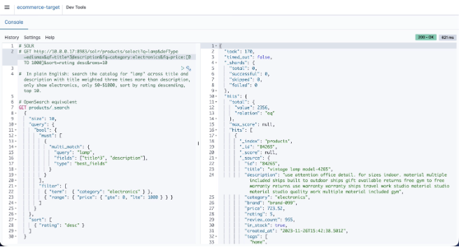
To follow along, open Dev Tools and run one of the translated queries from the assessment: a multi-field text search with a field boost, a category filter, a price range, and a sort. The Solr version of that query, in its native URL form:
GET /solr/products/select?q=lamp&defType=edismax&qf=title^3 description&fq=category:electronics&fq=price:[0 TO 1000]&sort=rating desc&rows=10
The translation is mechanical: Solr’s q=lamp becomes a multi_match clause, fq filters become bool.filter entries, and sort keeps the same shape. The following screenshot shows both queries side by side in Dev Tools, along with the OpenSearch response.
Figure 10: OpenSearch Dashboards Dev Tools showing the translated OpenSearch query and its response, returning 2,356 matching documents
The response shows 2,356 matching documents returned in 170 milliseconds, with the top hits sorted by rating, all queryable through the new OpenSearch Serverless endpoint.
Updating your application code
The Migration Assistant moves your data and schema, and it can also mirror live Solr traffic to the target during migration. The capture proxy records requests to your source, and the replayer sends them to OpenSearch using the SolrToOpenSearchTransformProvider you configured earlier. It reads your Solr schema and solrconfig.xml to translate queries in a field-type-aware way. That translation covers common Solr query and update patterns. It returns an error on features it doesn’t support rather than translating them incorrectly, so check the Migration Assistant documentation for the current list of supported behavior. This path is built for migration and cutover validation, not as a permanent production query layer. Because Solr and OpenSearch differ in query syntax, request handlers, and response shape, you still rewrite your application’s query layer for production. Two AI-driven paths are available:
AWS Transform is a collaborative IT transformation workbench that accelerates cloud migration, application modernization, and technical debt reduction. AWS Transform delivers high-quality, repeatable transformations without requiring specialized automation expertise. You can also handle the refactoring using available development tools your team uses for application development to help rewrite the relevant Solr client calls to use the OpenSearch client.
An AI coding assistant can also handle the refactoring. Any AI coding assistant that your team uses for application development can read your repository and rewrite the relevant Solr client calls to use the OpenSearch client. For better results, AWS provides integration tools that help. These tools reference AWS documentation and include Solr to Amazon OpenSearch Service capabilities that the Migration Assistant uses. This approach is less structured than AWS Transform but can be done with your existing development tools.
As you plan the query rewrite: devise a strategy for each of the following areas:
Query parser differences – Solr’s eDisMax qf/pf/bf/bq/mm don’t map 1:1 to OpenSearch. multi_match with type: best_fields or most_fields is the closest analogue, but boost math (bf) and phrase-field boosting (pf) require rewrites.
Request handler configs – Solr solrconfig.xml request handlers (with defaults, appends, invariants) become search templates or application logic on OpenSearch.
Response format – Solr’s response.docs compared to OpenSearch’s hits.hits.
Function queries and score modifications – Solr’s _val_, bf, and function query syntax must be rewritten as function_score or script_score. Semantics are close but rarely identical, and BM25 compared to Solr’s TF-IDF (or BM25 in newer Solr) produces different absolute scores.
Faceting – Solr facet.field, facet.range, and facet.pivot become OpenSearch aggregations.
Highlighting, fl field selection, and cursorMark pagination – All have OpenSearch equivalents with different names and semantics.
Bonus: Improve search relevance with Automatic Semantic Enrichment
After your data lands in an OpenSearch Serverless collection, you have access to capabilities that weren’t available on Solr such as vector based search and semantic enrichment. One option is Automatic Semantic Enrichment. Automatic Semantic Enrichment uses a pre-trained sparse encoder (opensearch-neural-sparse-v2) to expand each document with weighted co-occurring terms at indexing time. It then matches incoming queries against the expanded representation. You get relevance improvements without hosting a model or running inference at query time.
Consider a query like “durable rain jacket” against a product catalog. A keyword-only search returns documents that contain those literal words. With Automatic Semantic Enrichment activated, the same query also surfaces related items like waterproof shells, hardshells, and weatherproof coats, without anyone writing or maintaining synonym files. Automatic Semantic Enrichment is configured at index creation time and can’t be activated by changing the mapping afterward. After activation, sparse vectors are generated automatically for every ingested document. The AI assistant will help you set up a semantically enriched field as part of the migration.
Cost
The Migration Assistant infrastructure costs approximately $0.40–0.70 per hour while running. The target OpenSearch Serverless collection has a separate baseline cost. OpenSearch Serverless can scale compute to zero when idle, so you pay only for storage when the collection is not handling requests, and it provisions faster than previous generations.
Clean up
When you finish testing, remove the resources you created so you don’t keep paying for them:
Delete the AWS CloudFormation stack MigrationAssistant-<stage>, which removes the VPC, NAT gateway, Amazon EKS cluster, Amazon ECR repository, and IAM roles it created.
Empty and delete the Amazon S3 bucket that holds the snapshot and the captured traffic tuples.
Delete the Kubernetes secret solr-basic-auth and remove the container images from the Amazon ECR repository.
Remove any temporary access you granted on the Solr source, and revoke the data access policy entry you added to the target OpenSearch Serverless collection.
Conclusion
The Migration Assistant reduces the manual engineering effort required to move from Apache Solr to Amazon OpenSearch Serverless. The Migration Assistant handles orchestration and guides you through assessment, backfill, and validation, while development tools can help reduce the effort needed to rewrite application code.
Try the Migration Assistant for Amazon OpenSearch Service in your own AWS account. Point it at a non-production Solr, Elasticsearch, or self-managed OpenSearch cluster and describe your goal in language, for example, “Deploy Migration Assistant in us-west-2 so I can start testing” or “Run the historical data migration for my Elasticsearch 7.10 cluster.” Run an assessment and take a workload through backfill and validation to see how the Assistant handles the process for you. As you use the Migration Assistant on your own projects, tell us what worked and where you encountered challenges, so we can keep improving the assessment, translation, and validation experience.
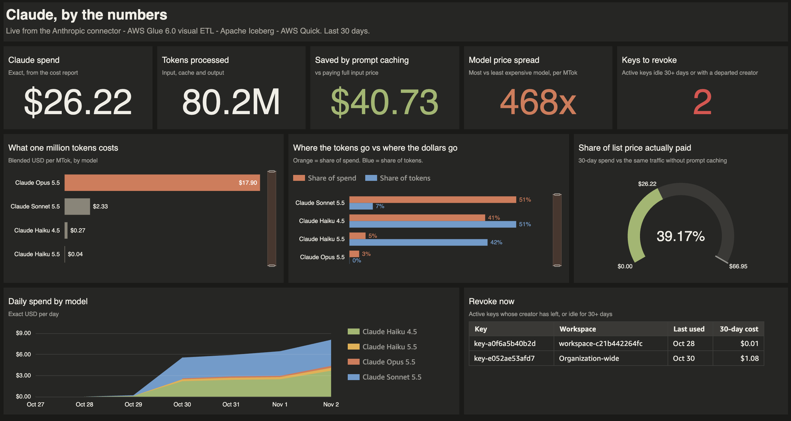
Finance teams want to allocate AI spend to the business units that use it. Engineering leaders want to know what that spend delivers. Security teams want to know who owns each API key and whether any belong to former employees. Anthropic gives administrators detailed visibility into usage and cost through Claude Code usage analytics and the Anthropic Admin API. Many enterprises want to take the next step and analyze that data alongside the business data they already manage in AWS. Until now that has meant building and maintaining a custom integration with the Admin API.
AWS Glue now offers a native connector for Anthropic. AWS Glue is a serverless data integration service that helps you discover, prepare, move, and integrate data from multiple sources for analytics, artificial intelligence and machine learning (AI/ML), and application development. The connector for Anthropic is one of 100 new native connectors that AWS Glue added for popular software as a service (SaaS) applications. It works like other AWS Glue connectors and requires no custom code. You store an Anthropic API key in AWS Secrets Manager and create an AWS Glue connection that references it. The connector handles the API calls and schema mapping for you so your team can focus on analyzing the data instead of maintaining the integration.
The connector makes AI usage another domain in your data lakehouse. With Amazon S3 Tables, fully managed Apache Iceberg tables in Amazon Simple Storage Service (Amazon S3), you can store your transformed Anthropic and business data in an open and interoperable format that AWS analytics services can read natively and other Iceberg engines can query.
In this post, we follow the fictional retailer AnyCompany Retail as it brings Anthropic data into Amazon S3 Tables and joins it with its own business data using AWS Glue materialized views stored as Apache Iceberg tables. The team uses Amazon Athena to query the data with SQL and answer leadership’s three questions about spend, value, and API key ownership. It then publishes the results to an AWS Quick dashboard that leadership reviews every week.
Solution overview
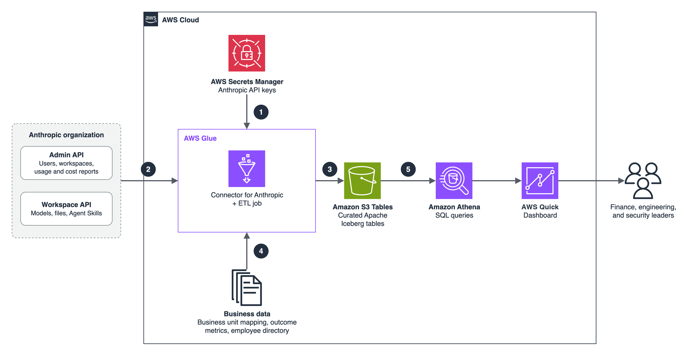
The following diagram shows the solution architecture.
Figure 1: Solution architecture for analyzing Anthropic usage data with AWS Glue, Amazon S3 Tables, Amazon Athena, and AWS Quick
The workflow consists of the following steps:
You store your Anthropic API keys in AWS Secrets Manager, where the AWS Glue connection references them.
An AWS Glue extract, transform, and load (ETL) job uses the Glue connector for Anthropic to read entities such as usage and cost reports, users, and workspaces.
The job transforms the data into fact and dimension tables like daily usage, daily cost, and writes them to Amazon S3 Tables as Apache Iceberg tables.
The job joins the Anthropic data with business data that you own like workspace-to-business-unit mapping, outcome metrics, and an employee directory. In our example, this data is stored in Amazon S3.
Amazon Athena queries the tables to answer the spend, value, and access questions, and AWS Quick presents the results through natural language prompting or dashboards.
Supported entities
Anthropic uses two kinds of API keys, and each provides access to different sets of data. An Admin API key reads organization-level data. A workspace API key reads data inside a single workspace. You create one AWS Glue connection for each key.
Entity
API key
Description
users
Admin
Organization members with their email, name, and role
invites
Admin
Pending and accepted organization invites
workspaces
Admin
Workspaces in the organization, including the default and archived workspaces
workspace_members
Admin
Members of each workspace with their workspace role
api_keys
Admin
API keys with status, scope, workspace, and creator
usage_report
Admin
Token usage per time bucket, optionally grouped by workspace, API key, model, and more
cost_report
Admin
Cost per daily bucket, optionally grouped by workspace and cost description
models
Workspace
Claude models available to the workspace
message_batches
Workspace
Message Batches API jobs with status and request counts
files
Workspace
Files uploaded to the workspace
Example scenario
The retailer uses Claude across five business units, each with its own Anthropic workspace: Customer Service, Engineering, Document Processing, Marketing, and Data Science. Every week, leadership reviews AI spend across the business units and asks three questions:
Which business units are driving AI spend?
Is the spend paying off, for example in cost per resolved customer case?
Are any active API keys owned by employees who have left the company?
Throughout this post, the Anthropic data comes from a demo organization. The reference datasets (business-unit mapping, support outcomes, and employee directory) are illustrative samples.
Prerequisites
To follow along, you need the following:
An Anthropic organization (Admin API features aren’t available for individual accounts).
An Anthropic Admin API key, created by an organization admin.
A workspace API key for each workspace you want to analyze.
An AWS account with AWS Identity and Access Management (IAM) permissions to use AWS Glue, Amazon Athena, Amazon S3, Amazon S3 Tables, AWS Secrets Manager, and AWS Quick.
An IAM role for AWS Glue with access to the secrets, your S3 bucket, and your S3 table bucket (see Part 2).
An S3 bucket for job scripts and reference data.
Part 1: Set up the AWS Glue connector for Anthropic
In this part, you store your Anthropic API keys in AWS Secrets Manager and create the AWS Glue connections that read your organization’s data.
Store your Anthropic API keys
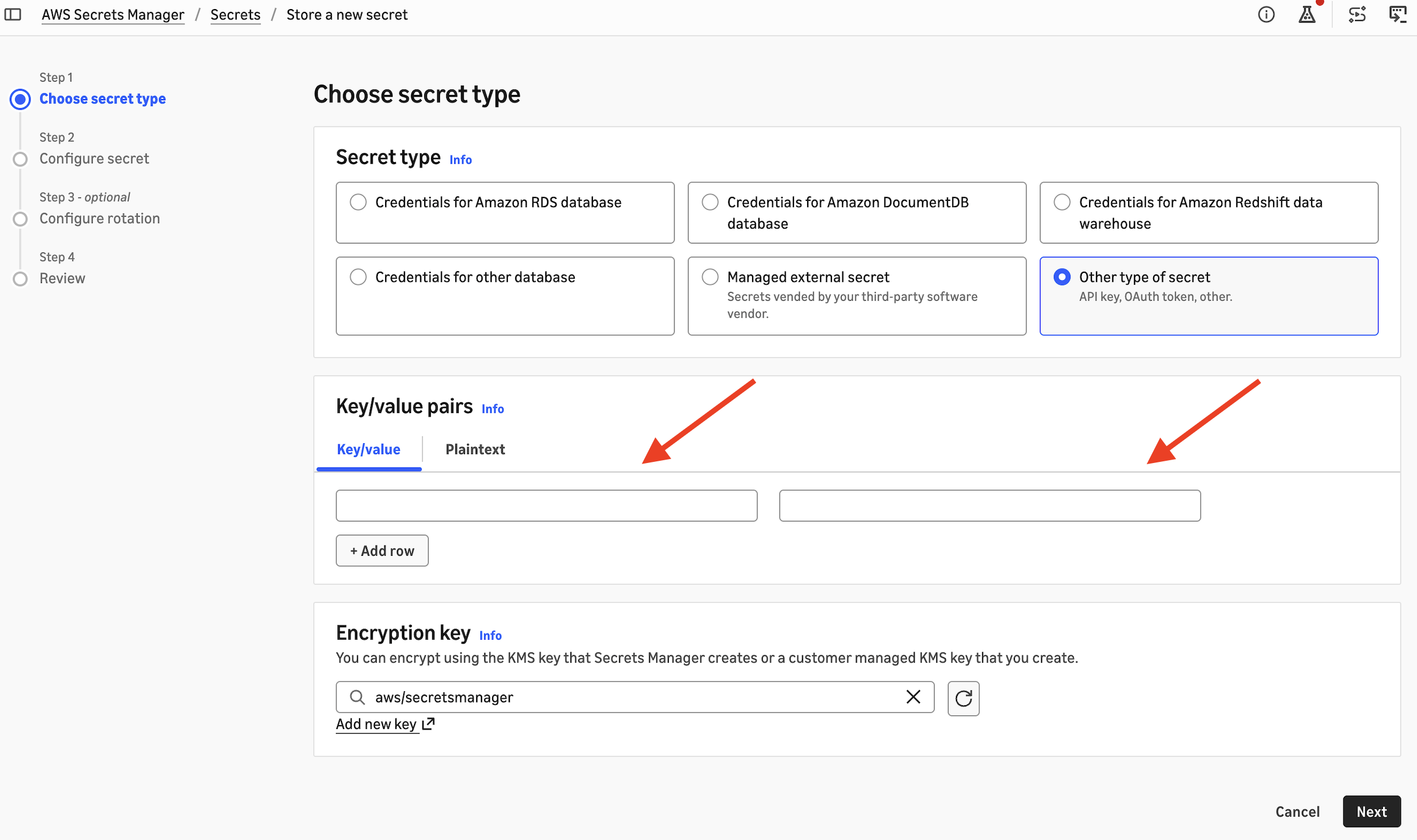
Store each API key in AWS Secrets Manager as a secret with the key apiKey:
{ "apiKey": "<your-anthropic-api-key>" }
Create one secret for the Admin API key and one for each workspace API key you plan to use.
Open AWS Secrets Manager.
Choose Store a new secret and enter your API key.
Figure 2: Storing an Anthropic API key in AWS Secrets Manager
Choose Next and name your new secret.
Optionally, configure automatic rotation.
Afterwards, choose Next and then Store.
Create the connections
On the AWS Glue console, choose Data connections, then Create connection.
For Data source, choose Anthropic.
Figure 3: Choosing Anthropic as the data source in AWS Glue
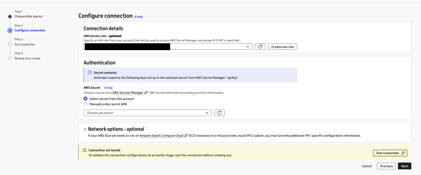
For Authentication, choose the secret that contains your Admin API key.
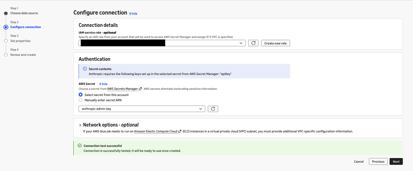
Figure 4: Selecting the secret that holds the Admin API key
Name the connection, for example anthropic-admin, and create it.
Repeat the steps with a workspace API key to create a second connection, for example anthropic-workspace.
After you create a connection, choose Test connection to validate the API key. Both Admin and workspace API keys can be validated.
Figure 5: Validating an Anthropic connection with Test connection
Explore and preview data
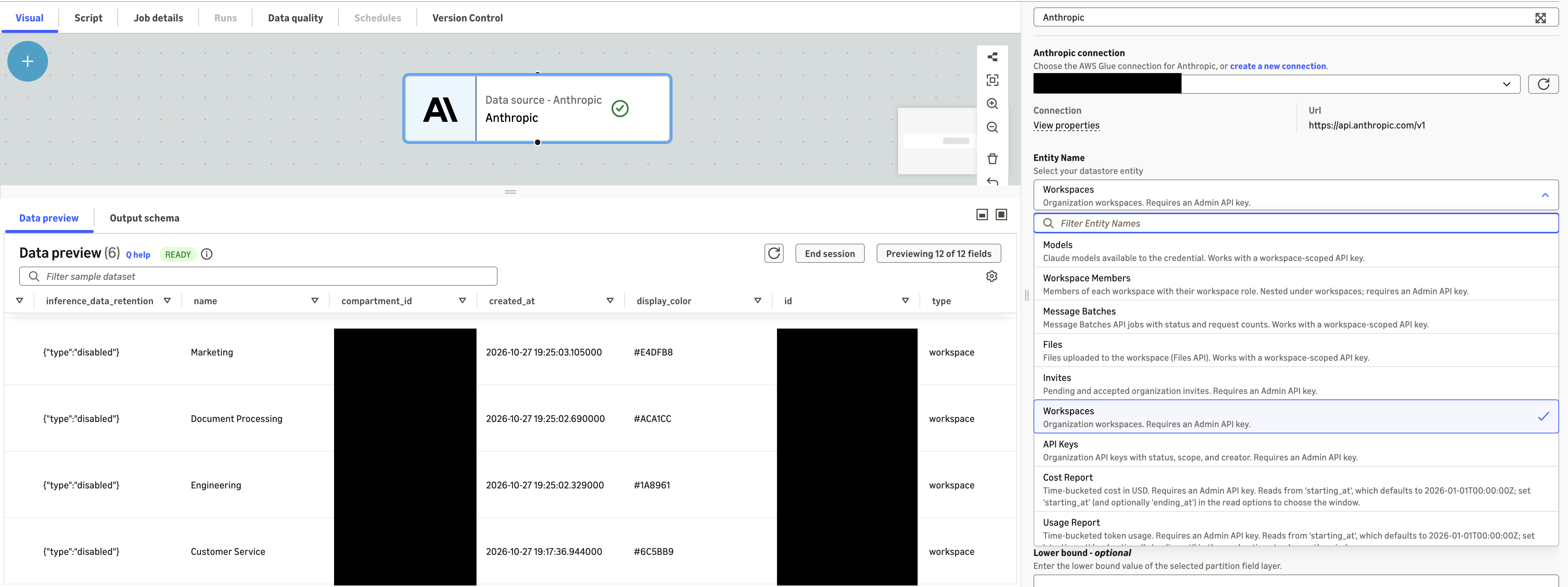
In the AWS Glue console, you can browse the entities that each connection exposes and preview records and the schema for all the data available through the AWS Glue connector for Anthropic. The following screenshot showcases synthetic data.
Figure 6: Previewing Anthropic entities and schema in the AWS Glue console
Part 2: Build an AI usage lakehouse with Amazon S3 Tables and AWS Glue materialized views
In this part, you turn the Anthropic data from Part 1 into answers to leadership’s three questions. An AWS Glue ETL job reads Anthropic data through the connector, combines it with your business data, and writes Apache Iceberg tables to Amazon S3 Tables. A second AWS Glue job maintains AWS Glue materialized views in the AWS Glue Data Catalog, one for each question, and you query the views with Amazon Athena.
The table bucket organizes the data in four namespaces:
Namespace
Contents
Written by
raw
Anthropic entities, as the connector returns them
ETL job
reference
Business data that you own, loaded from CSV files in Amazon S3
ETL job
curated
Daily fact tables and dimension tables, built from the raw data
ETL job
mart
Materialized views, one for each business question
Materialized view job
To build the pipeline, you complete the following steps.
Create the table bucket and namespaces
Create a table bucket, and then create one namespace for each layer:
aws s3tables create-table-bucket --name amzn-s3-demo-table-bucket

for ns in raw curated reference mart; do
  aws s3tables create-namespace \
    --table-bucket-arn arn:aws:s3tables:<region>:<account-id>:bucket/amzn-s3-demo-table-bucket --namespace "$ns"
done
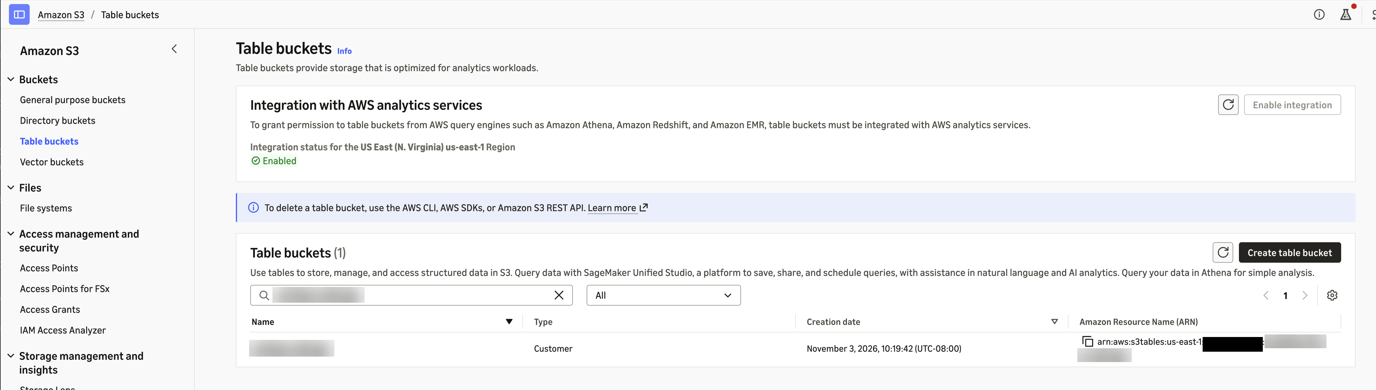
On the Amazon S3 console, choose Table buckets and enable Integration with AWS analytics services. The integration adds your table buckets to the AWS Glue Data Catalog under the s3tablescatalog catalog, so AWS Glue and Athena can address this bucket as s3tablescatalog/amzn-s3-demo-table-bucket. This walkthrough uses IAM access control for the integration.
Figure 7: Turning on AWS analytics integration for the table bucket
Upload your business data to Amazon S3
Anthropic data shows what each workspace and API key spends. It doesn’t show which business unit owns a workspace, what the spend produced, or whether the creator of a key still works at the company. That context lives in your own systems, so you create these datasets from your organization’s data. The datasets you need depend on the questions you want to answer. This post uses the following three sample datasets:
Save each dataset as a CSV file with a header row. In your S3 bucket, upload each file to its own folder under a common prefix, and name each folder after its dataset:
Pass itself to AWS Glue. Grant iam:PassRole on the role’s own ARN for glue.amazonaws.com, because AWS Glue stores the role with each materialized view and uses it to refresh the view.
Review the ETL script
The ETL job runs the script anthropic_usage_etl.py. Download anthropic_usage_etl.py and save it on your computer. You upload it when you create the AWS Glue job in a later step.
On each run, the script does the following:
Reads the cost report, usage report, users, workspaces, and API keys through the Admin connection, and message batches and files through any workspace connections that you list. It writes this data unchanged to the raw namespace.
Reads your business data from the Amazon S3 location in the --reference_data_path job parameter and writes it to the reference namespace.
Flattens the usage and cost reports into daily fact tables, converts cost from cents to US dollars, and builds tables of API keys, users, and workspaces in the curated namespace.
Creates any table that doesn’t exist yet and adds columns when the source data gains new fields, so you don’t need to create tables in advance.
The following snippets show three important parts of the script: how it reads data through the connector, how it builds the curated tables, and how it loads new data incrementally.
Read Anthropic data through the connector
The connector reads data directly into Apache Spark DataFrames through CatalogConnectionHelper, a helper library included with AWS Glue. You pass the connection type, the AWS Glue connection name, and the read options. For every read option and the fields that support filter pushdown, see Anthropic connection options. The following example reads the cost report from October 1, grouped by workspace and cost description:
from connectivity.adapter import CatalogConnectionHelper

connector = CatalogConnectionHelper(spark)

def read_entity(entity, connection, filter_predicate=None):
    """Read one Anthropic entity through the AWS Glue connection into a Spark DataFrame."""
    options = {"ENTITY_NAME": entity}
    if filter_predicate:
        options["FILTER_PREDICATE"] = filter_predicate
    return connector.read("anthropic", connection, options) # connection type, connection name, options

def read_report(entity, starting_at, group_by):
    """Read a usage or cost report from starting_at, broken down by the group_by dimensions."""
    conditions = [f"starting_at = '{starting_at}'"] + [f"group_by = '{field}'" for field in group_by]
    report = read_entity(entity, "anthropic-admin", " AND ".join(conditions))
    return report.select("starting_at", "ending_at", "results")

cost_report = read_report("cost_report", "2026-10-01T00:00:00Z", group_by=["workspace_id", "description"])
read_report builds the filter predicate from the start date and group_by dimensions, and keeps the report columns that the job uses. The result is a Spark DataFrame, so you can use it with standard Spark transformations without converting it. The job reads cost_report and usage_report with read_report and users, workspaces, and api_keys with read_entity.
Workspace entities, such as message_batches and files, need a workspace API key, so the job reads them through each workspace connection that you list in the --workspace_connections job parameter. The job writes everything that it reads, unchanged, to the raw namespace.
Build the curated tables
The connector returns the cost report as one record per day. That record holds all of the day’s cost lines in a single field, results, as a JSON array. To analyze individual cost lines, the job parses results with a schema for the cost line fields (COST_LINE_SCHEMA) and expands the array, so that each cost line becomes its own row. Anthropic reports cost amounts in cents, so the job converts them to US dollars. Anthropic also reports activity in the Default workspace with an empty workspace_id, so the job fills in the Default workspace ID:
def build_fact_cost_daily(cost_report, default_workspace_id):
    """One row per day, workspace, and cost line, with the amount converted from cents to US dollars."""
    return (
        cost_report
        .withColumn("line", F.explode(F.from_json("results", COST_LINE_SCHEMA)))
        .select(
            F.to_date("starting_at").alias("cost_date"),
            # Anthropic reports Default workspace activity with an empty workspace_id
            F.coalesce("line.workspace_id", F.lit(default_workspace_id)).alias("workspace_id"),
            "line.description",
            "line.model",
            "line.cost_type",
            "line.token_type",
            "line.currency",
            (F.col("line.amount").cast("decimal(20,8)") / 100).alias("amount_usd"),
        )
        .groupBy(*COST_KEYS)
        .agg(F.sum("amount_usd").alias("amount_usd"))
    )
The job also parses nested fields such as the API key creator, scope, and principal. It writes the following tables to the curated namespace:
Table
Contents
fact_usage_daily
Token usage per day, workspace, API key, and model
fact_cost_daily
Cost in US dollars per day, workspace, and cost line
dim_api_key
API keys with status, workspace, creator, and key type (linked to a user, service account, or legacy)
dim_user, dim_workspace
Organization members and workspaces
Load new data incrementally
The first run loads all data from the date in the --start_date job parameter. Later runs re-read only the last three days, because daily buckets close after midnight UTC and recent days can still change. The job merges those days into the fact tables, so a rerun updates rows instead of duplicating them:
MERGE INTO s3tables.curated.fact_cost_daily t
USING updates s -- the re-read days
ON t.cost_date <=> s.cost_date AND t.workspace_id <=> s.workspace_id
AND t.description <=> s.description AND t.model <=> s.model
AND t.cost_type <=> s.cost_type AND t.token_type <=> s.token_type
AND t.currency <=> s.currency
WHEN MATCHED THEN UPDATE SET *
WHEN NOT MATCHED THEN INSERT *;
The dimension and reference tables are small, so the job replaces them on every run.
Review the materialized view script
The materialized view job runs the script anthropic_usage_mvs.py. Download anthropic_usage_mvs.py and save it on your computer.
The curated tables hold clean usage, cost, and access data, but each leadership question needs joins across several of them and your business data. Instead of repeating those joins in every query and dashboard, the script saves each answer as a materialized view in the mart namespace. A materialized view stores the result of a query as an Iceberg table. When its base tables change, a refresh updates the view, incrementally where possible, instead of recomputing the whole query. Athena and AWS Quick then read the precomputed results, so everyone works from the same numbers.
On each run, the script creates any view that doesn’t exist yet and refreshes the rest. It maintains one view for each leadership question:
Are any active API keys owned by employees who have left?
Add your own views
The script is extensible. Each view is one entry in the VIEWS dictionary: the key is the view name, and the value is the view’s SQL query. To answer a new question, add an entry. For example, the following entry adds a view of daily token usage by workspace and model:
VIEWS = {
    # ... the three views in the preceding table ...
    # Which models consume the most tokens in each workspace?
    "tokens_by_model": f"""
        SELECT u.usage_date,
            w.name AS workspace,
            u.model,
            sum(u.uncached_input_tokens) AS uncached_input_tokens,
            sum(u.cache_read_input_tokens) AS cache_read_input_tokens,
            sum(u.output_tokens) AS output_tokens
        FROM {CURATED}.fact_usage_daily u
        LEFT JOIN {CURATED}.dim_workspace w ON w.workspace_id = u.workspace_id
        GROUP BY 1, 2, 3
    """,
}
The next run of the job creates the view, and later runs refresh it. To change the definition of an existing view, set the optional --recreate job parameter to the view name, for example tokens_by_model, for one run. The job drops the view and creates it again with the new definition.
Follow two rules when you write a view definition:
Make definitions deterministic. Functions such as current_date() aren’t allowed, so calculate those values at query time.
Use inline subqueries instead of a WITH clause. In our testing, views that used a WITH clause could be created but failed to refresh.
Create the AWS Glue jobs
Create one AWS Glue job for each script. Both jobs connect to the table bucket with the same job parameter, so prepare its value first.
Prepare the table bucket configuration
The scripts read and write the table bucket through an Apache Spark catalog named s3tables. You configure the catalog with one job parameter, --conf. Copy the following value as a single line, and replace <account-id>, <region>, and amzn-s3-demo-table-bucket with your own values:
The value contains several Spark settings. AWS Glue accepts only one --conf parameter, so the settings are separated by --conf inside the value. With this configuration, the scripts refer to tables as s3tables.<namespace>.<table>, for example s3tables.curated.fact_cost_daily. For details about these settings, see Running ETL jobs on Amazon S3 tables with AWS Glue.
Create the ETL job
On the AWS Glue console, choose ETL jobs, and then choose Script editor.
For Engine, choose Spark. Choose Upload script, select anthropic_usage_etl.py, and choose Create script.
On the Job details tab, for Name, enter anthropic-usage-etl. For IAM Role, choose the role from the prerequisites. For Glue version, choose Glue 6.0.
Expand Advanced properties. Under Connections, choose the Admin connection and each workspace connection that you created in Part 1.
Under Job parameters, choose Add new parameter and add each of the following keys and values:
Key
Value
Purpose
--datalake-formats
iceberg
Adds Apache Iceberg support to the job
--conf
The value that you prepared
Connects the job to the table bucket
--admin_connection
anthropic-admin
Name of the Admin connection
--workspace_connections
{"anthropic-workspace": "Customer Service"}
Optional. Maps each workspace connection to its workspace name. Without it, the job skips message_batches and files.
--reference_data_path
s3://<your-bucket>/<prefix>/
Location of your business data
--start_date
2026-10-01
First day to load on the first run
Choose Save.
Create the materialized view job
On the AWS Glue console, choose ETL jobs, and then choose Script editor.
For Engine, choose Spark. Choose Upload script, select anthropic_usage_mvs.py, and choose Create script.
On the Job details tab, for Name, enter anthropic-usage-mvs. For IAM Role, choose the same role. For Glue version, choose Glue 6.0 (AWS Glue materialized views require AWS Glue 5.1 or later).
Expand Advanced properties. Under Job parameters, add --datalake-formats with the value iceberg, and --conf with the same value as the ETL job. This job reads only from the table bucket, so it doesn’t need connections or other parameters.
On the ETL jobs page, run anthropic-usage-etl. After it succeeds, run anthropic-usage-mvs, which creates the views on its first run and refreshes them on later runs.
To keep the views current, create an AWS Glue workflow that runs the ETL job daily at 06:30 UTC, after Anthropic’s daily buckets close, and then runs the materialized view job. Alternatively, add SCHEDULE REFRESH EVERY 24 HOURS to each CREATE MATERIALIZED VIEW statement so that AWS Glue refreshes the views on a schedule, and schedule only the ETL job.
Answer the business questions with Amazon Athena
After you execute the following Glue scripts, in the Athena query editor, choose the catalog s3tablescatalog/amzn-s3-demo-table-bucket and the database mart. The results in this section come from the demo organization. The business datasets are samples.
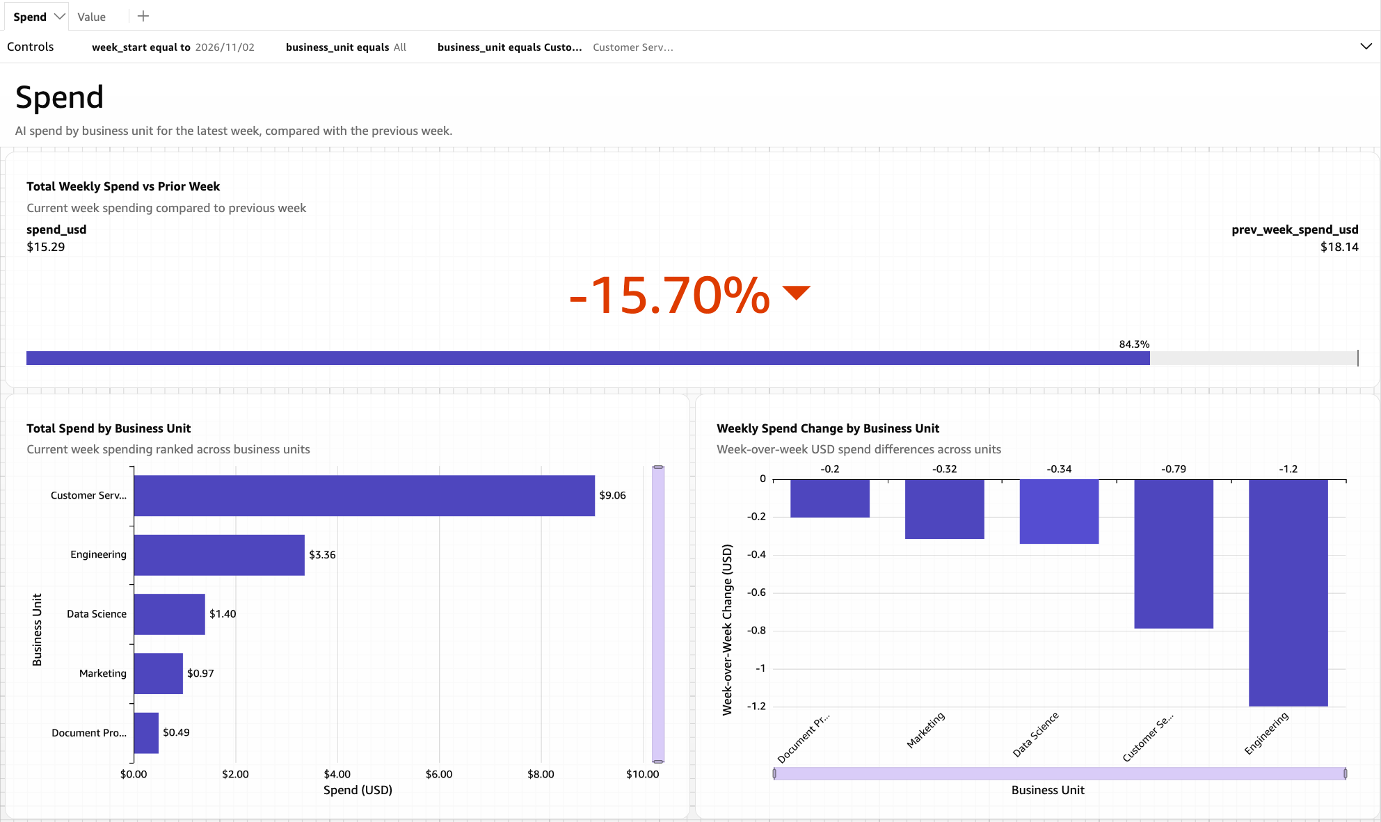
Which business units are driving AI spend?
SELECT week_start, business_unit, spend_usd, prev_week_spend_usd
FROM weekly_spend_by_business_unit
WHERE week_start = (SELECT max(week_start) FROM weekly_spend_by_business_unit)
ORDER BY spend_usd DESC;
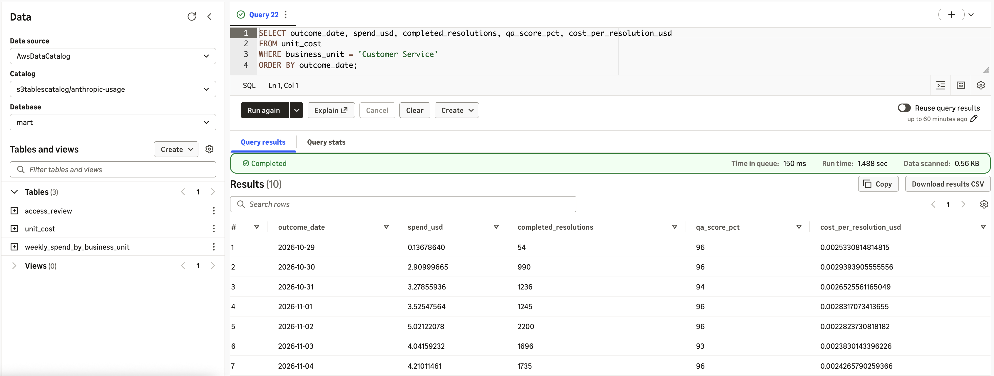
Is the spend paying off?
SELECT outcome_date, spend_usd, completed_resolutions, qa_score_pct, cost_per_resolution_usd
FROM unit_cost
WHERE business_unit = 'Customer Service'
ORDER BY outcome_date;
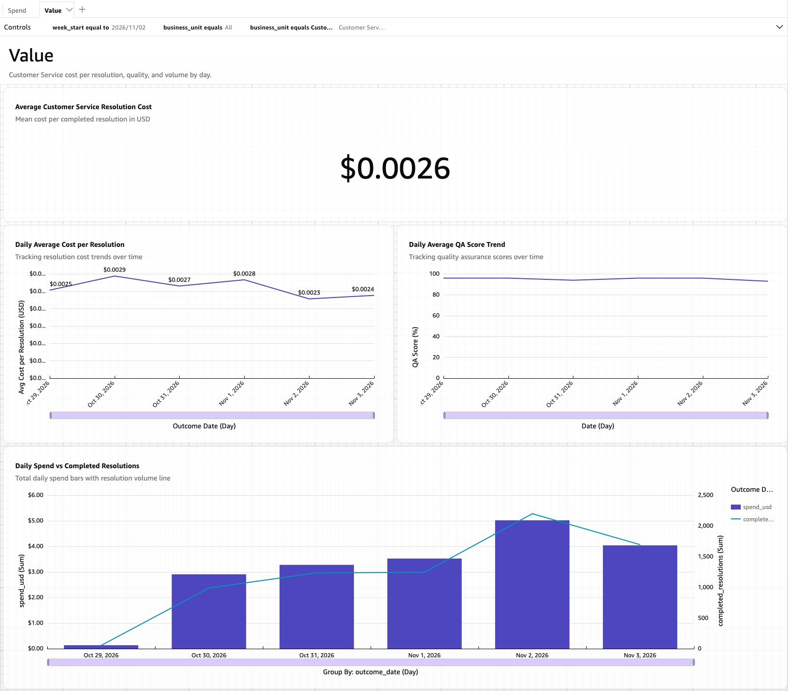
Figure 8: Cost per resolution over time for Customer Service
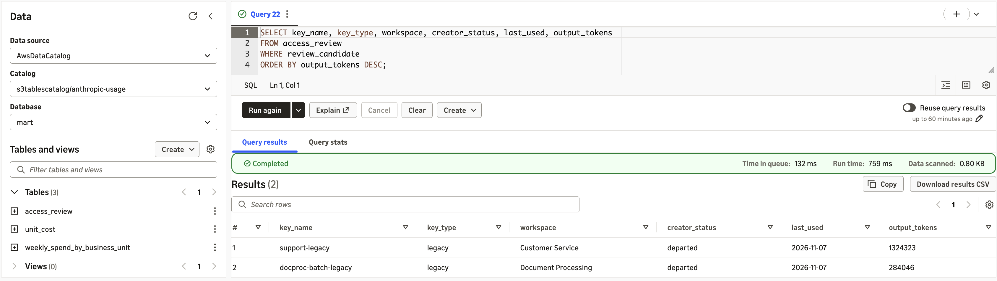
Are any active API keys owned by employees who have left?
SELECT key_name, key_type, workspace, creator_status, last_used, output_tokens
FROM access_review
WHERE review_candidate
ORDER BY output_tokens DESC;
Figure 9: Active API keys owned by employees who have left
The query returns two keys, support-legacy in Customer Service and docproc-batch-legacy in Document Processing. Both are legacy keys, created by an employee who has since left, and both were used the previous day. A departed creator doesn’t mean that a key is misused. It identifies keys whose service ownership should be confirmed, for example by moving the workload to a service-account key, before the old key is disabled.
Part 3: Visualize AI spend and governance in AWS Quick
AWS Quick is a generative AI assistant for work. It helps employees find insights, conduct deep research, automate tasks, and take action across their business applications, bringing chat agents, research, workflow automation, and business intelligence (BI) together in one place. Its BI capability, AWS Quick Sight, turns data into interactive dashboards. With generative BI, you can build a multi-sheet dashboard from a natural language prompt or ask questions of your data in plain language.
Allow AWS Quick to access the table bucket
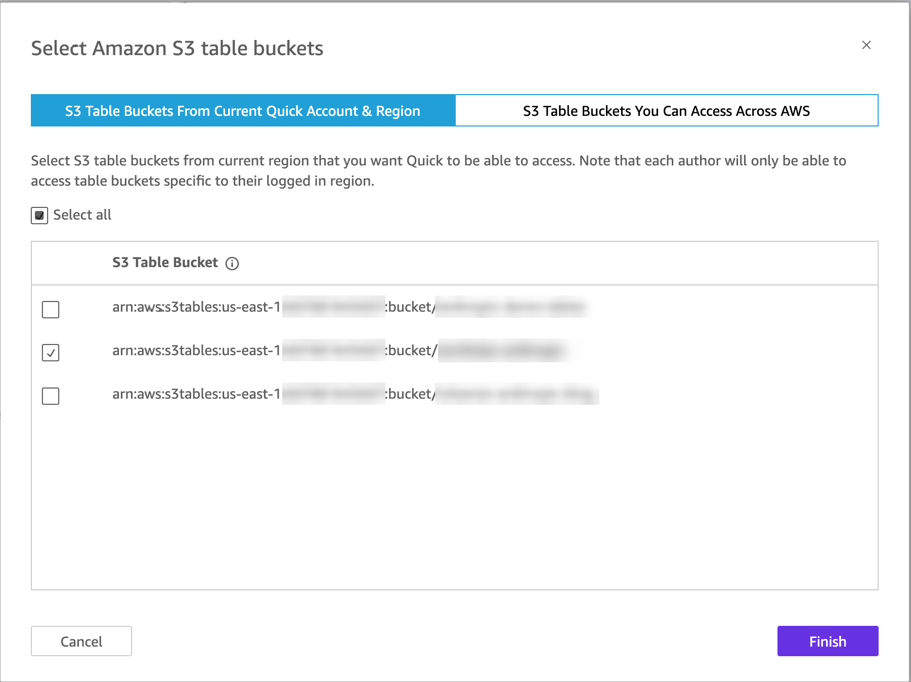
AWS Quick reads materialized views directly from the table bucket. Before you create a dataset, an AWS Quick administrator allows Quick to access the bucket:
In AWS Quick, open Manage account.
Under Permissions, choose AWS resources.
Select Amazon S3 Tables, choose Select S3 table buckets, select the amzn-s3-demo-table-bucket table bucket, and choose Finish.
Figure 10: Granting AWS Quick access to the table bucket
Without this step, creating the data source fails with a message that AWS Quick doesn’t have permission to access the database.
Create datasets from the materialized views
Create one dataset for each view that the dashboard uses:
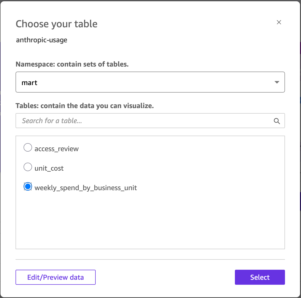
Choose Data, then Create dataset, and then Create data source.
Choose Amazon S3 Tables. Enter a data source name, such as anthropic-usage, and the table bucket ARN, for example arn:aws:s3tables:<region>:<account-id>:bucket/amzn-s3-demo-table-bucket. Choose Create data source.
For Namespace, choose mart. Select weekly_spend_by_business_unit and choose Select.
Choose Directly query your data, and then Edit/Preview data. Check the preview and choose Save & publish.
Repeat these steps for unit_cost, and select the anthropic-usage data source that you created instead of creating a new one.
Figure 11: Creating datasets from the materialized views in AWS Quick
Because the datasets query the views directly, the dashboard shows the latest results after each refresh of the materialized views. You don’t need a separate refresh schedule in AWS Quick.
Generate the analysis from a prompt
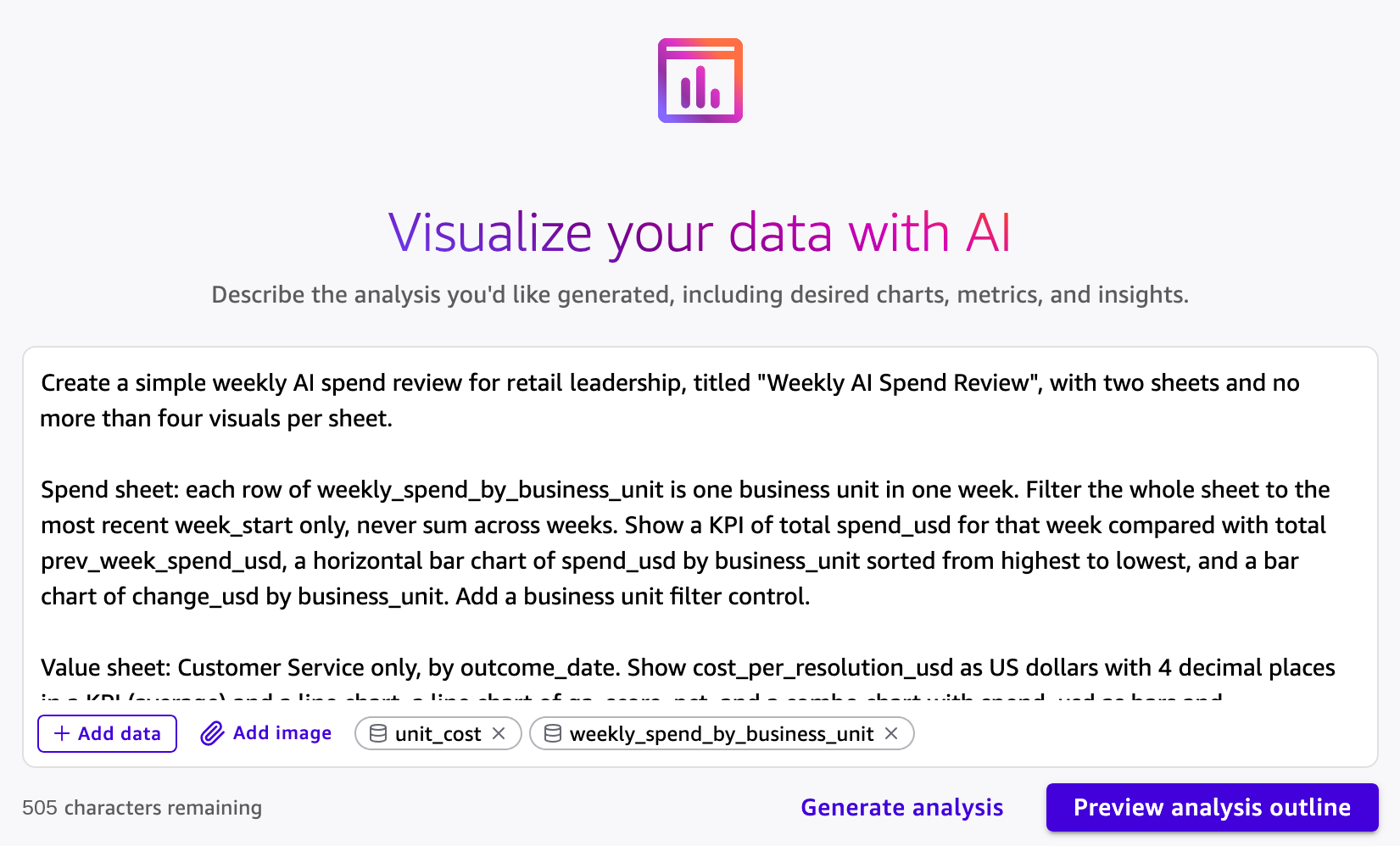
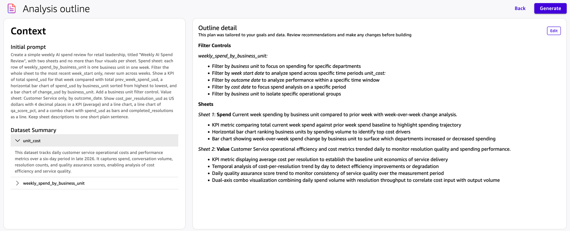
Instead of building each visual by hand, describe the review that leadership wants and let AWS Quick generate the analysis. On the Analyses page, choose Generate analysis. Choose Add data, select both datasets, and enter a prompt such as the following:
Create a simple weekly AI spend review for retail leadership, titled "Weekly AI Spend Review", with two sheets and no more than four visuals per sheet.

Spend sheet: each row of weekly_spend_by_business_unit is one business unit in one week. Filter the whole sheet to the most recent week_start only, never sum across weeks. Show a KPI of total spend_usd for that week compared with total prev_week_spend_usd, a horizontal bar chart of spend_usd by business_unit sorted from highest to lowest, and a bar chart of change_usd by business_unit. Add a business unit filter control.

Value sheet: Customer Service only, by outcome_date. Show cost_per_resolution_usd as US dollars with 4 decimal places in a KPI (average) and a line chart, a line chart of qa_score_pct, and a combo chart with spend_usd as bars and completed_resolutions as a line.

Keep sheet descriptions to one short plain sentence.
Figure 12: Generating the analysis from a natural language prompt
Choose Preview analysis outline. AWS Quick reviews the columns and statistics of each dataset and proposes a plan with filter controls, sheets, and the visuals on each sheet. Review the plan, choose Edit if you want to change it, and then choose Generate.
Figure 13: Previewing the proposed analysis outline
Describe the shape of your data in the prompt. The weekly_spend_by_business_unit view has one row per business unit per week. When our first prompt only asked to compare spend with the previous week, the generated analysis added all weeks together. Asking for the most recent week only fixed it.
Review the dashboard
The Spend sheet shows which business units are driving AI spend.
Figure 14: The Spend sheet showing AI spend by business unit
The Value sheet shows whether the spend is paying off.
Figure 15: The Value sheet showing whether the spend is paying off
Publish and share the dashboard
Choose Publish to create a dashboard from the analysis, and share it with leadership. Viewers can filter and explore the dashboard without access to the analysis or the datasets behind it. To have the review arrive before the weekly meeting, schedule an email report from the dashboard.
Go further
This dashboard answers leadership’s questions with two datasets and a short prompt, but the same connector data supports much more. For advanced use cases, use the Agent Toolkit for AWS with your preferred AI coding agent to build a richer version of this solution through natural language. The following dashboard compares the price per million tokens across models, shows how much prompt caching saves, and lists the API keys to revoke. We generated the entire data pipeline and this dashboard with Kiro and the Agent Toolkit for AWS.
Figure 16: A richer dashboard built with the Agent Toolkit for AWS
Considerations
Report time windows: Set starting_at for every usage and cost read. Daily buckets include only completed days. Use bucket_width = '1h' for the current day.
API key scope: An Admin API key reads organization data but not workspace data such as models, message batches, or files, and a workspace API key reads only its workspace. Use one connection per key, and one set of connections per Anthropic organization.
Rate limits: The Anthropic Admin API limits request rates. Use bounded time windows and scheduled incremental reads rather than large historical reads.
AWS Glue materialized views: AWS Glue materialized views require AWS Glue 5.1 or later and iam:PassRole for the role that refreshes them. Definitions must be deterministic, and in our testing views with a WITH clause failed to refresh, so use inline subqueries.
Security: Grant the AWS Glue role read access only to the secrets it needs, rotate Anthropic API keys regularly, and restrict access to curated tables.
Clean up
To avoid ongoing charges, delete the resources you created: the AWS Glue jobs, workflow, and connections. The Secrets Manager secrets. The materialized views, tables, namespaces, and table bucket in Amazon S3 Tables. The reference data and scripts in Amazon S3. You can also remove the dashboards and datasets that you created in AWS Quick. Consider revoking any Anthropic API keys you created for this walkthrough.
Conclusion
In this post, we showed how to use the AWS Glue connector for Anthropic to bring Anthropic usage, cost, and access data into AWS, store it as Apache Iceberg tables in Amazon S3 Tables, and keep business-ready results current with materialized views. With Amazon Athena, the retailer can see which business units drive AI spend, whether that spend pays off, and which API keys need an ownership review. Using AWS Quick, we used natural language to create dashboards.
To get started, see Anthropic connection options in the AWS Glue Developer Guide. To browse the other connection types that AWS Glue supports, including the new native connectors for SaaS applications, see Available connections.
Today, we are announcing updates to the AWS Well-Architected Framework with new and improved guidance across its six pillars, Operational Excellence, Security, Reliability, Performance Efficiency, Cost Optimization, and Sustainability. The Framework now separates account- and organization-level best practices from workload best practices, so you can establish foundational guardrails in the environment where your workloads run. New best practices address secure coding, cyber resilience for backup data, generative AI for operational efficiency, and measuring resource efficiency, so the Framework reflects how teams build and operate in the cloud today.
A brief history
The AWS Well-Architected Framework is a collection of best practices that organizations of every size and industry use to design, build, and operate workloads that are secure, reliable, high-performing, cost-effective, sustainable, and straightforward to operate.
We launched the first version of the Framework in 2012. Since then, it has grown from a single set of guidance into a full body of architectural knowledge. We published the AWS Well-Architected Framework whitepaper, added the Operational Excellence pillar, and released pillar-specific whitepapers and AWS Well-Architected Lenses for specific technologies and industries. Next, we refreshed the Framework so that best practices became the core unit of guidance, and we added Sustainability as the sixth pillar. As customers began building with generative and agentic AI, we introduced new lenses to guide them. In 2026, the Framework continues to change to help customers build and run secure, resilient, efficient, and sustainable workloads in the cloud.
Figure 1: AWS Well-Architected guidance timeline, 2012 to 2026.
What’s new
Customers tell us they value Well-Architected reviews and want a more efficient way to run them. Account- and organization-level best practices apply across the entire environment, so customers want to assess them once and then focus each review on the workload itself. To streamline reviews, this release organizes the Framework into two areas, Well-Architected Cloud Foundations and Well-Architected Cloud Workloads. As a result, a workload review covers only the best practices that apply to that workload, which makes it faster to run and automate.
Well-Architected Cloud Foundations covers environment-wide decisions, such as multi-account structure, identity, and cost governance. It sets the guardrails that every workload inherits, and you refine them as your environment matures. Well-Architected Cloud Workloads covers how you design, build, and operate each workload, including updated architecture patterns focused on specific business outcomes. In both areas, best practices are organized into capabilities, which are groups of related best practices that share a common objective.
This release focuses on technical architecture. As more teams use AI agents to run reviews, guidance is most useful when an agent can check it against how your environment and workloads are built and operated. Best practices centered on business strategy, people, and organizational processes depend on human judgment and context that are not captured by configuration or telemetry. Mixing these elements with technical guidance makes it more difficult to automate reviews. We retired these best practices, and AWS continues to offer guidance on these topics through other resources. Each remaining best practice now addresses a technical decision that you, or an agent acting on your behalf, can review and act on.
We also updated service references throughout the Framework, removing services that no longer accept new customers or have reached end of support, and adding guidance for services launched since the last release.
Well-Architected Cloud Foundations
Best practices for account- and organization-level decisions were previously spread across the Framework and reviewed for every workload. Well-Architected Cloud Foundations consolidates them into guidance you apply when you set up or mature your multi-account environment. Of the best practices in Well-Architected Cloud Foundations, 33 come from moving or merging existing best practices from the Framework pillars.
We consolidated and rewrote the relocated best practices from an environment-wide perspective, then combined them with newly authored foundational guidance. That guidance includes new best practices for centralized event monitoring, an auditable cloud inventory record, and centralized DNS management. The result is 45 best practices across seven capabilities: Multi-account environment, Identity and access management, Central observability management, Resource and inventory management, Security and compliance, Cloud financial management, and Networking and connectivity.
Well-Architected Cloud Workloads
Well-Architected Cloud Workloads now has 216 best practices, down from 307, with no loss of technical coverage, so each workload review stays focused on its architecture decisions. Practices that apply across your environment moved into Well-Architected Cloud Foundations, practices with similar guidance were combined, and practices outside the technical scope of the Framework were retired.
Operational Excellence
Operational Excellence introduces new capabilities and best practices that follow the operations lifecycle, which covers observation, deriving insights, managing change flow, deployment, support, response, and evolution. It adds a new best practice for managing rollouts of external dependencies and expands guidance on using AI assistants and agents to instrument telemetry, draft dashboards, and investigate incidents, with validation against baselines and named human ownership at every step.
Security
Security moves account-wide concerns, such as root account protection, sign-in mechanisms, permission guardrails, emergency access, centralized logging, and forensic readiness, into the Identity and access management and Security and compliance capabilities of Well-Architected Cloud Foundations. Within Well-Architected Cloud Workloads, the pillar adds new best practices for centralized workload permissions management, detection metrics and dashboards, and secure coding guidelines.
Reliability
Reliability moves three networking best practices (IP subnet allocation, hub-and-spoke topologies, and non-overlapping address ranges) into the Networking and connectivity capability of Well-Architected Cloud Foundations, where they are consolidated into a single network strategy best practice. Within Well-Architected Cloud Workloads, the pillar adds a new best practice on cyber resilience for backup data, which helps protect backups against ransomware and other cyber threats.
Performance Efficiency
Performance Efficiency moves its best practice on policies and reference architectures into Well-Architected Cloud Foundations. Within Well-Architected Cloud Workloads, the pillar now focuses Architecture selection on validating your workload requirements and tracking them with key performance indicators (KPIs). It also combines related best practices, such as folding compute configuration into compute selection and load testing into workload performance evaluation.
Cost Optimization
Cost Optimization moves its best practices on account-level concerns, such as account structure, cost attribution, billing tools, and cost controls, into Well-Architected Cloud Foundations, where they form the core of the Cloud financial management capability. Within Well-Architected Cloud Workloads, the pillar combines overlapping best practices, such as merging its decommissioning guidance into a single resource lifecycle management best practice. It also adds a new best practice on using generative AI for operational efficiency.
Sustainability
Sustainability introduces new capabilities and best practices that follow how teams reduce workload impact, which covers measuring and monitoring, provisioning resources, improving workload efficiency, and optimizing data and processing. Based on customer feedback, earlier general guidance has been converted to best practices. It adds a new best practice for using the most resource-efficient computational approach, including using a less resource-intensive method or a smaller machine learning model where one meets the requirement. It expands guidance on combining resource usage efficiency metrics with carbon emissions data from the AWS Sustainability Console / API and AWS Data Exports, with baselines and targets that make progress measurable over time.
Call to action
AWS Well-Architected Framework is more than a set of best practices and tools for finding improvement opportunities. It is a mechanism that helps you strengthen governance and drive better outcomes across your organization. When you evaluate your architecture consistently against best practices, you build a culture of continuous improvement and address critical issues before they affect your workloads. Ready to get started? Explore the updated AWS Well-Architected Framework, soon to be available in 11 languages: English, Spanish, French, German, Italian, Japanese, Korean, Indonesian, Brazilian Portuguese, Simplified Chinese, and Traditional Chinese.
An Apache Flink application that runs operations such as aggregations, joins, and windows builds up state as it processes events, and Amazon Managed Service for Apache Flink saves that state in snapshots. Until now, a snapshot belonged to the application that created it, so you could restore it only into that same application, in the same Region.
Today, we’re announcing general availability of enhanced snapshots. An enhanced snapshot is an AWS resource with its own Amazon Resource Name (ARN), decoupled from the application that created it. You can start a different application from it in the same account and Region. You can also export it to an Amazon Simple Storage Service (Amazon S3) bucket you own. In the other direction, you can import an Apache Flink savepoint from Amazon S3 as a new enhanced snapshot and start an application from it.
With enhanced snapshots, you can deploy updates to a stateful application without a long pause in processing, recover in a second Region, and move a self-managed Flink job to the managed service with its state. In this post, we walk through these three use cases. We then show how to turn on enhanced snapshots, start one application from another’s state, export and import snapshots, and set up permissions. For the full reference, see Enhanced snapshots in the Amazon Managed Service for Apache Flink Developer Guide.
Use cases
These three use cases all build on the same concept: making an application’s state reusable across applications.
Support blue/green deployments for stateful applications
Deploying new code to a stateful application normally means stopping it, restarting it from a snapshot, and waiting while the new version catches up. A blue/green deployment avoids a long outage and reprocessing all the data. You run the current version (blue) and the new version (green) side by side, and you keep blue running until you have checked green’s output. For a stateful application, the hard part is bootstrapping green from blue’s existing state, and that is what enhanced snapshots provide.
Take an enhanced snapshot of blue, then start green from that snapshot with the new code. Green begins with blue’s state and processes only the data written since the snapshot. When green has caught up, point downstream consumers at its output and stop blue. If green has a problem, blue is still running.
While both run, each application reads the source and writes its own output, and you pay for the compute of both. Green reprocesses the events written since the snapshot, so its output overlaps with blue’s. Downstream consumers must tolerate duplicates or deduplicate them when you cut over, because this pattern doesn’t give you exactly-once delivery across the switch. You can also use the same flow to A/B test a change against production state, or to clone a running application’s state to reproduce a bug without touching the live job.
Disaster recovery in a second Region
If a Region becomes unavailable, a standby application in another Region can take over with recent state. It doesn’t need to start empty and rebuild its state from the source. Export and import run in the Region where the snapshot lives. To recover in a second Region, export snapshots on a schedule to a bucket in the primary Region. Then replicate that bucket to the standby Region with Amazon S3 Cross-Region Replication. When you need to fail over, import the latest replicated snapshot in the standby Region and start the standby application from it. More frequent exports mean less data to process after failover and a faster recovery, at the cost of more export operations and more Amazon S3 storage and replication. Choose the export interval from your recovery time objective (RTO).
Migrate a self-managed Apache Flink application with its state
Moving a self-managed Flink job to a managed service means starting it with empty state and replaying history to rebuild it. With enhanced snapshots, the job moves together with its state. Take a savepoint of the job on your self-managed Flink cluster. Copy it to an S3 bucket in the account and Region where the new application will run. Import the savepoint as an enhanced snapshot, then start an Amazon Managed Service for Apache Flink application from it.
Import validates the savepoint before it restores, so the source objects must meet the documented requirements, including a full-object CRC-64/NVME (CRC64NVME) checksum. See the Developer Guide for the full list of import prerequisites.
The new application starts from the savepoint’s state and resumes reading the source from the savepoint’s offsets. It processes only the data written since the savepoint instead of replaying history. For the import to work, the savepoint must come from a supported Flink version and your job’s operator IDs (UIDs) must match the ones in the savepoint. Check the new application’s output before you shut down the self-managed job. An imported snapshot has no source application, so it does not appear when you list snapshots by application name. Track the snapshots you import by calling ListSnapshots with SnapshotInitiatorOperation set to ImportSnapshot when you need them for cleanup or inventory.
How it works
Because an enhanced snapshot is an AWS resource of its own, separate from the application that created it, it has its own IAM permissions, which the last step covers.
Turning on enhanced snapshots and restoring from them takes a handful of API calls and one new application setting. The following steps cover each one, from turning on the feature through the permissions you need. The examples use the AWS Command Line Interface (AWS CLI). If you receive errors when running AWS CLI commands, make sure that you’re using the most recent version of the AWS CLI. If you work with a coding agent, the Agent Skill described at the end of this post gives it the same guidance.
Turn on enhanced snapshots
Enhanced snapshots work with applications on Apache Flink 1.20 and later. For a new application, set SnapshotMode to ENHANCED_SNAPSHOTS in ApplicationSnapshotConfiguration when you create it. You can switch an existing application in place while it is running, and it keeps its state:
You can undo the switch with RollbackApplication, but only before you update the application again. After that, you can’t change the mode back. Once you switch, CreateApplicationSnapshot returns an error, so move any scripts that you use to periodically take snapshots of the application to CreateSnapshot first. Take an enhanced snapshot right after you switch, because that is the application’s first snapshot that another application can start from or that you can export.
Snapshot creation is asynchronous. Call describe-snapshot until SnapshotStatus is READY. The response also returns the SnapshotArn. Then start the green application, created with enhanced snapshots turned on, from that ARN:
RESTORE_FROM_CUSTOM_SNAPSHOT already exists for application snapshots, which you select with SnapshotName. For an enhanced snapshot, you pass SnapshotArn instead. The new application restores the saved state only if its operator UIDs, state types, and maxParallelism are compatible with the job that wrote the snapshot. It must also run a compatible Flink version.
Enhanced snapshots stay until you delete them with DeleteSnapshot, including after you delete the application that created them.
Export and import
Export and import read from and write to your bucket through an IAM role that you pass in the request. The service assumes that role, so the Amazon S3 permissions belong on the role rather than on the caller. The role’s trust policy allows the kinesisanalytics.amazonaws.com service principal, scoped with aws:SourceAccount and aws:SourceArn. The bucket must be in the same account and Region as the snapshot. For the full trust and permissions policies for these roles, see Export and import permissions in the Developer Guide.
End KeyPrefix with a slash. Each export writes to a new folder under the prefix, and the service reports the exact location as ExportedPrefix when you describe the operation. When you import an exported snapshot, point KeyPrefix at that exact folder, not at the parent prefix. The import looks for the savepoint metadata there, and a prefix that does not contain it fails.
To import a savepoint copied from a self-managed cluster:
To import a snapshot you exported instead, set KeyPrefix to its ExportedPrefix.
Both calls are asynchronous and return a SnapshotOperationId. Track progress with describe-snapshot-operation, which also returns error details if the operation fails:
Export and import use AWS Key Management Service (AWS KMS) keys for both the snapshot and the S3 objects. Specify each key as a full key ARN, because key IDs and aliases are rejected. For key policies, encryption settings, and the encryption context, see Encryption for enhanced snapshots in the Developer Guide.
Set up permissions
Enhanced snapshots are their own IAM resource type, with ARNs of the form arn:aws:kinesisanalytics:region:account-id:snapshot/snapshot-name. Two of the new actions are permission-only, with no API of the same name, so you might overlook them. With kinesisanalytics:RestoreFromSnapshot on the snapshot ARN, a caller can start, update, or roll back an application from a snapshot, including a snapshot the same application created. kinesisanalytics:CreateSystemSnapshot on the application ARN covers the automatic snapshots the service takes when you stop, update, or start an application that has snapshots turned on. Keep it in the policy even if you never stop the application, because the start path checks it too.
With the following policy, a caller can run one application, snapshot it, and start from its snapshots:
The orders-enrichment-* pattern matches the snapshots you create, assuming you start their names with the application name. The SYSTEMSNAPSHOT-*–orders-enrichment-* pattern matches the system snapshots the service takes for this application. This policy scopes to a single application. A blue/green or migration setup that starts a second application needs the same StartApplication and CreateSystemSnapshot grants on that application’s ARN too. System snapshots inherit the application’s tags, and you can scope access by tags with aws:ResourceTag conditions on the snapshot actions. ListSnapshots lists across the account, so its resource is *. Leave out the KMS statement if the application uses an AWS owned key. For export and import, the caller also needs kinesisanalytics:ExportSnapshot or kinesisanalytics:ImportSnapshot on the snapshot ARN, and iam:PassRole for the role, scoped with iam:PassedToService set to kinesisanalytics.amazonaws.com.
Now available
Enhanced snapshots are available today in all AWS Regions where Amazon Managed Service for Apache Flink is available, for applications on Apache Flink 1.20 and later. For the number of export and import operations you can run at a time, see Quotas in the Developer Guide.
Enhanced snapshot storage is priced the same as application snapshots, and there is no additional charge for export or import. Amazon S3 charges for storage, requests, and replication in your own buckets. Enhanced snapshots and the system snapshots the service takes on stop, update, and start are kept until you delete them. They keep accruing storage charges after the application that created them is gone, so delete snapshots you no longer need. To learn more, visit the Amazon Managed Service for Apache Flink pricing page.
To get started, see Enhanced snapshots in the Amazon Managed Service for Apache Flink Developer Guide.
If you use a coding agent, install the developing-applications-on-managed-service-for-apache-flink Agent Skill with the AWS CLI. For setup details, see the Agent Toolkit for AWS Skill Installation Guide. For example:
We also recommend that you install the AWS MCP Server in your developer tool of choice. It gives coding agents tools to search AWS documentation, blog posts, and Agent Skills at runtime. They can then work from current AWS guidance and find and install skills more easily. To install it, see Setting up the AWS MCP Server.
On November 6, 2026, the Apache Software Foundation disclosed CVE-2026-90436, a critical unsafe reflection vulnerability (CWE-470) in Axis 1.x that allows for unauthenticated remote code execution (RCE). Apache Axis is a Simple Object Access Protocol (SOAP) implementation used for the creation of Java Web services. CISA has assigned CVE-2026-90436 a CVSS score of 9.8 Critical.
Since the initial November 6 disclosure, it has transpired that some versions of Atlassian Confluence Data Center and N-able N-central use the affected Axis library and are vulnerable to CVE-2026-90436. Both products require a non-default configuration in order to be vulnerable.
CVE-2026-90436 is now being actively exploited in the wild against both known affected products. On November 13, 2026, Rapid7 MDR detected exploitation of CVE-2026-90436 against Atlassian Confluence Data Center in a customer environment. Separately, on November 13, 2026, N-able reported exploitation in the wild against N-central for a vulnerability that strongly correlates to CVE-2026-90436. A proof-of-concept exploit that leverages CVE-2026-90436 and targets N-central was published on November 12, 2026, as part of a series of public zero-day disclosures against N-central.
Rapid7 recommends remediating exposed systems on an emergency basis outside of normal patching cycles.
MDR observed exploitation
On November 13, 2026, Rapid7’s MDR team responded to a surge of alerts firing on the abnormal child processes launched by an Atlassian Confluence server. A review of the Confluence access logs revealed unauthenticated POST requests to /plugins/servlet/soap-axis1/confluenceservice-v2, each returning an HTTP 500 (Internal Server Error). Despite the error responses, endpoint telemetry showed Confluence’s Java process launching Bash and curl as the dedicated confluence service account, within seconds of these requests. The attacker proceeded to run hundreds of hex-encoded shell commands and scripts fetched from temporary Pinggy and Cloudflare Tunnel domains. Each command wrapped its output in labeled delimiters, and carried sequential task IDs, a structure that suggests the use of AI-assisted automated tooling.
From this foothold, the attacker enumerated the host, network, Confluence configuration, encryption keys, and database settings. Just over three minutes after the first observed execution, the attackers were authenticating to MySQL with Confluence’s own database credentials, querying page bodies, application links, and attachments with names associated with credentials, tokens, VPN configurations, and private keys. The attacker’s scripts, likely AI-generated, then targeted files in Confluence’s default location for uploaded page attachments (/var/atlassian/application-data/confluence/attachments/v4/), parsed Office documents, searched for credentials, and hunted for payment card numbers, using Luhn checks to filter out false positives.
The attacker continued extensive enumeration, mapping various internal services. They used a Confluence application credential to query the internal Atlassian Crowd API for users and group memberships, then ran Impacket’s GetNPUsers.py against a domain controller, attempting an AS-REP roasting attack.
Although these attempts failed, the access we did observe relied on credentials stored in Confluence, and roughly four hours after the first exploit request, the attacker had acquired a service account credential and began querying a production cloud data warehouse. Approximately twelve hours after the first exploit request, the attacker signed in to Microsoft 365 as an integration service account using legacy authentication from 192.238.253[.]176. The same address appeared in the hostname of the Pinggy tunnel and in exploit requests observed earlier in the intrusion.
Mitigation guidance
Prioritize internet-accessible instances with the relevant APIs enabled, and check internal deployments as well. Apply the product-specific actions below, then investigate systems that were exposed for evidence of compromise.
Axis 1.x through 1.4 is affected but has reached end of life (EOL) and Apache does not plan to publish a fixed Axis 1.x release. Apache recommends moving to another SOAP engine (for example, Apache Axis 2) or using an Axis 1.x build with this patch applied. Organizations using products that are affected by this issue should follow the product vendor’s specific remediation instructions.
Atlassian Confluence Data Center
Atlassian lists versions 1.x through to 9.x as affected when “Remote API (XML-RPC & SOAP)” is enabled. Version 9.2.28 is the fixed release. The setting has been off by default for new installations since version 3.0. Confluence version 10.x and later removed the feature so are not vulnerable, and Atlassian Cloud is unaffected.
Affected users should upgrade to version 9.2.28 or a current unaffected 10.x release. If patching must wait, an administrator can open “General Configuration” and “Further Configuration”, edit the settings, clear “Remote API (XML-RPC & SOAP)”, and save. The change takes effect without restarting Confluence, but integrations using the API may stop working.
Follow the Confluence advisory for the latest fixes and mitigation instructions.
N-able N-central
On-premises administrators should confirm that “Legacy API” is disabled, even on 2026.4 HF2. N-able states that it is off by default, and provides instructions for disabling Legacy API. Its November 13 guidance says hosted environments received temporary protections directly; customers in both hosting models must still follow the vendor’s Agent and Probe upgrade guidance. N-able also temporarily disabled the Intune integration as a precaution. Refer to the N-able security update for these responsibilities.
Update: On November 16, 2026, N-able released N-central 2026.4 HF3 (2026.4.1.39) which addresses multiple issues including seventeen new CVEs. The “Legacy API” feature which exposed the vulnerable CVE-2026-90436 Axis attack surface has been disabled in this new release. N-central users should upgrade to N-central 2026.4 HF3 on an emergency basis outside of normal patching cycles.
Follow the N-able advisory for the latest fixes and mitigation instructions.
IOCs
The presence of these IOCs in logs should prompt investigation, but the absence of these addresses does not confirm that an environment was unaffected.
Atlassian Confluence Data Center
The following IP addresses and domains are associated with observed exploitation of CVE-2026-90436 against Atlassian Confluence Data Center:
192.238.253[.]176
5.133.47[.]243
163.182.68[.]109
104.13.106[.]166
*.trycloudflare[.]com
wpefh-192-238-253-176.free.pinggy[.]net
webhook[.]site
N-able N-central
N-able’s November 13 incident update lists these IP addresses as IOCs for N-central customers who had not disabled Legacy API.
157.20.241[.]16
139.99.69[.]109
79.76.51[.]56
The vendor’s update also lists associated URLs for use in compromise assessment.
Updates
November 16, 2026: Initial publication.
November 17, 2026: Updated Remediation section for N-central.
November 17, 2026: Added the MDR observed exploitation section and updated IOCs.
A second delivery of the same message can reveal more about an application than its happy-path demo. I like tools that make those cases easier to investigate while a change is still small. Last week’s launch of AWS Emulator brings part of that work onto your own machine: developers and coding agents can exercise AWS API interactions, inspect results, and try again without provisioning cloud resources for every attempt.
I wrote about the Emulator’s launch last week, and it’s my main highlight in this edition. There are also new ways to isolate workloads on shared infrastructure, give an agent narrowly scoped access to a backend, and prepare search applications for a regional disruption. Now, let’s get into this week’s AWS news…
AWS Emulator runs locally alongside your code and development tools. Image: AWS.
Headlines Test your applications against AWS locally with AWS Emulator introduces a generally available local environment for AWS API interactions. Point the AWS CLI or AWS SDKs at its HTTPS endpoint, and your application keeps its normal SDK calls. The walkthrough shows a coding agent creating an Amazon DynamoDB table, writing an item, and reading it back. You don’t need an AWS account for emulated operations, and there is no additional service fee. The getting-started guide covers Linux packages, Docker for macOS and Windows, and agent-assisted setup; the source is on GitHub.
What I like is giving an agent concrete feedback while it works: run calls, inspect results, and revise the code. Matt Wood’s perspective on feedback for coding agents explores why that loop matters. Check the published fidelity results for your operations, because coverage varies and unimplemented calls return HTTP 501. The emulator doesn’t reproduce IAM and resource-policy enforcement or cross-account and cross-Region behavior, so test the complete application and its security configuration on AWS before production.
AWS Nitro Sandboxes bring hardware isolation to pods, tasks, and VMs. You can give an Amazon EKS pod or Amazon ECS task its own VM boundary while sharing an Amazon EC2 instance. That is useful for tenant workloads, build jobs, and agents executing generated code. Isolated mode separates workloads from their neighbors; confidential mode adds protection from node operators and cryptographic attestation. The Compute Blog deep dive explains both modes and their integrations. Nitro Sandboxes have no additional charge on supported instances; EC2 and applicable EKS Auto Mode or ECS Managed Instances fees still apply.
Last week’s launches Here are some launches and updates from this past week that caught my attention:
Amazon Cognito supports OAuth 2.0 token exchange – You can now exchange a user’s token for one scoped to a downstream service in Amazon Cognito. The derived token can have narrower permissions and a single audience, with no refresh token; supplying an actor token also identifies the intermediary in an act claim. For an agent calling a backend on someone’s behalf, that makes delegation more explicit without forwarding the original token. The feature is available on Essentials and Plus plans in all Cognito Regions.
Claude Fable 5.2 is available on AWS – You can access the model through Amazon Bedrock or Claude Platform on AWS. Anthropic positions it as its most capable generally available model for technical work, including extended engineering tasks, scientific research, and quantitative finance. Bedrock has model-specific retention requirements: Fable 5.2 traffic is retained for up to 30 days for abuse detection, with a temporary zero-retention exception for eligible internal use.
Amazon ElastiCache Serverless adds search and aggregations – You can now combine vector, full-text, and hybrid search with server-side aggregations in Amazon ElastiCache Serverless for Valkey. That gives product discovery, recommendations, and agent-memory retrieval another option for querying frequently changing data. The capability requires Valkey 9, so create a compatible cache or upgrade an existing one. It is available in commercial Regions, AWS GovCloud (US), and the AWS European Sovereign Cloud.
Amazon OpenSearch Service adds managed cross-Region disaster recovery – You can now pair Amazon OpenSearch Service domains running version 3.7 or later in two Regions within one account. AWS specifies recovery objectives under one minute for data loss and under 20 minutes for recovery time. Planned switchovers preserve all writes; unplanned failovers can lose unreplicated data. The deep dive covers the remaining work: keeping configuration aligned and redirecting application writes after switching roles, plus secondary-domain and data-transfer charges.
Amazon CloudWatch Logs adds account-level retention policies – You can now set retention across all log groups or groups matching a name prefix in Amazon CloudWatch, with policies covering existing groups or only new ones. When policies overlap, the longest retention period applies. A platform team can set a baseline and retain security logs longer without updating every group individually. The feature has no additional charge and is available in commercial Regions except Middle East (Bahrain) and Middle East (UAE).
The next generation AgentCore runtime is now the default – New Amazon Bedrock AgentCore runtimes now use the next-generation runtime by default, so agent sessions start in under 2 seconds, scale up to 8 vCPU and 32 GB, scale to zero when idle, and bill up to 68% less memory, while each session still runs in its own isolated microVM.
For a full list of AWS announcements, be sure to keep an eye on the What’s New with AWS page.
Other AWS news Here are some additional posts and resources that you might find interesting:
Optimizing cost per task and proving agent ROI on Amazon Bedrock – This guide follows an agent’s cost through repeated calls, reasoning, caching, and human review. I like its emphasis on measuring a completed task and comparing outcomes against a documented baseline. Its worked prices are illustrative; use your own workload and reconcile estimated costs with billing data.
How Zillow runs 100 million daily notifications on AWS Step Functions – Zillow describes reusable content modules and configuration-driven AWS Step Functions Express Workflows for more than 100 million daily notifications. The useful engineering details include idempotent modules, batching, campaign isolation, and testing expressions with the TestState API before deployment. Those patterns apply well beyond notification systems.
Upcoming AWS events Check your calendar and sign up for upcoming AWS events:
AWS re:Invent – Join the community in Las Vegas from November 30 to December 4. Browse more than 2,200 sessions, including workshops and deep dives, or register for the free livestream to follow keynotes and selected sessions remotely.
AWS Community Days – Find community-led technical talks, workshops, and hands-on learning near you. Check each organizer’s page for current dates and registration details.
Join the AWS Builder Center to connect with builders, share solutions, and access content that supports your development. Browse here for upcoming AWS-led in-person and virtual events and developer-focused events.
That’s all for this week. Check back next Monday for another Weekly Roundup!
– Daniel Abib
This post is part of our Weekly Roundup series. Check back each week for a quick roundup of interesting news and announcements from AWS!
The FSI challenge: Faster delivery with stronger controls
Financial institutions face a difficult asymmetry. Frontier models can help defenders find and remediate weaknesses faster, but regulators are also warning that the same capabilities might accelerate vulnerability discovery and exploitation. The supervisory response is raising expectations for prioritized vulnerability management, continuous monitoring, operational resilience, supply-chain assurance, and the use of AI-based defensive tools under safeguards, human oversight, and robust risk management.
Traditional software delivery makes that harder. Build, security, risk, and operations often work in separate tools and review cycles, with context passed through tickets and manual handoffs. Security checks might occur late, evidence is assembled after the fact, and incident responders must reconstruct what changed across multiple systems. For regulated teams, this creates more than delay: it makes controls harder to apply consistently and decisions harder to evidence.
Under the Digital Operational Resilience Act (DORA), accountability for Information and Communication Technology (ICT) risk remains with the financial institution, including its use of cloud and other third-party providers. Fast development speed alone isn’t enough. Teams need a delivery model that shortens the cycle from discovery to remediation while retaining approval points, traceable evidence, and human accountability.
A governed AI-DLC with three Frontier Agents
The AI-Driven Development Lifecycle (AI-DLC) provides a practical pattern: an AI agent drafts or analyzes, a human evaluates, and the cycle repeats in short iterations. Applied across the lifecycle, agents can help author code, assess release readiness, identify security weaknesses, and investigate production failures. Humans continue to set policy, evaluate findings, authorize material changes, and own the production decision.
In this hands-on walkthrough, Kiro, AWS Security Agent, and AWS DevOps Agent work across a shared GitHub-based workflow. Kiro authors and revises code. AWS DevOps Agent reviews release readiness before and during the pull request. AWS Security Agent performs a deeper security review. A human approves the merge, and AWS DevOps Agent investigates production failures.
Under DORA, accountability for ICT risk stays with the financial institution regardless of which cloud or tooling it uses. Showing that every change was scanned, reviewed, and approved before it reached production, with evidence captured in the delivery toolchain itself, is what turns a good engineering practice into a defensible compliance posture. The institution moves faster without weakening the governance chain, because the agents handle the analysis while humans retain the authority over what gets deployed. This reference implementation doesn’t provide compliance by itself. Each institution must map it to its policies, segregation-of-duties requirements, model risk controls, risk appetite, and DORA obligations.
The three agents — role mapping across the SDLC
SDLC Phase
Agent
What it does
Plan → Build → Test
Kiro (autonomous agent)
Virtual developer. Maintains persistent context across sessions, learns from PRs and feedback. Handles multi-repo tasks: bug triage, code coverage, feature implementation. Connects to Jira, GitHub, Slack.
Virtual site reliability engineer (SRE), and now code reviewer. Release readiness code reviews on every change (cross-repo dependency risks, standards compliance, access control, automated verification testing), plus always-on incident triage, root cause identification and proactive reliability recommendations. Works with Amazon CloudWatch, Datadog, Dynatrace, Splunk, New Relic, Grafana, ServiceNow, Jenkins, GitHub.
Integration model: Workflow-level orchestration
The three agents operate as complementary autonomous systems that share the same software development lifecycle (SDLC) context through common tooling (repos, continuous integration and continuous delivery (CI/CD) pipelines, ticketing systems). The AWS DevOps Agent pulls double duty in this pipeline. Its release readiness code reviews capability makes it the first reviewer on every change: inside Kiro while the code is being written, and again on the PR, before it switches hats to incident response in production.
Figure 1: End-to-end workflow across Kiro, AWS DevOps Agent, and AWS Security Agent in a shared GitHub-based pipeline
Developer prompts Kiro on what to build. Kiro authors the code.
With the AWS DevOps Agent Kiro Power installed in Kiro, you can request a code release readiness review from AWS DevOps Agent right in the Kiro IDE. The release readiness review covers cross-repo dependency risks, standards compliance, access-control correctness, and automated verification testing.
After we pass the AWS DevOps Agent code readiness review, we push the code to GitHub from Kiro. The GitHub workflow is designed in a way that a Pull Request (PR) is automatically created.
AWS Security Agent runs the deeper OWASP / AWS Identity and Access Management (IAM) / secrets pass on the PR.
The developer might incorporate the output from AWS Security Agent and further revise the code. If all looks good, the developer merges the PR.
On merge, GitHub Actions deploys.
AWS DevOps Agent watches production and, the moment something breaks, opens an investigation, finds the root cause and ties back to the same GitHub repo Kiro is working in.
The rest of this post is the hands-on version of that loop: the exact wiring you need to make it run against a real repo.
Step-by-step setup
This section walks through the setup end to end, from a quick primer on GitHub Actions through the prerequisites and the six steps that wire the agents together.
A quick primer on GitHub Actions
GitHub Actions is GitHub’s built-in automation system. You drop YAML files into .github/workflows/ in your repo, and GitHub runs them on events you care about, such as a push, a PR being opened, a label being added, or a merge to main. Each workflow spins up a fresh Linux VM (“runner”), checks out your code, and executes a series of steps. Steps can be shell commands or reusable packages called actions. We use GitHub Actions as our CI/CD pipeline manager for demonstration purposes.
A Slack workspace (for AWS DevOps Agent notifications).
Prerequisite 2 — Install the GitHub Apps and connect the agents
GitHub Apps are the modern way to give automation identity and scoped permissions. For the general model, see About using GitHub Apps. For this demo, install the following on your repo:
The AWS DevOps Agent isn’t a GitHub App, but it needs three connections:
Connecting AWS DevOps Agent to GitHub – With GitHub integration, AWS DevOps Agent can access code repositories and receive deployment events during incident investigations.
(Optional)Connecting AWS DevOps Agent to Slack – With this connection, AWS DevOps Agent can post the investigation result to the designated Slack channel.
Step 1 — Author code in Kiro and push to GitHub
Kiro is an agentic IDE: you describe what you want to build, it writes and edits files, and you commit the result. Open your repo in Kiro, iterate until the feature works, then push a feature branch.
For demonstration purposes, we intentionally started with a flawed .py file with a hard-coded credential and a SQL injection vulnerability so the AWS DevOps Agent and AWS Security Agent have something to catch downstream. This is only to exercise the review agents end-to-end.
Because we installed the AWS DevOps Agent Kiro Power in Prerequisite 2, the review actually starts here, before anything is pushed. The Power includes Skills that tell Kiro to invoke a release readiness review after significant code changes and before creating a PR. Findings surface directly in the IDE, and Kiro offers to fix them on the spot. For this demo, we let the flawed file through so you can see the PR-side review catch it too.
Step 2 — Let the AWS DevOps Agent review the code
This is where the AWS DevOps Agent takes the first review pass. In this post, we use Kiro’s AWS DevOps Agent Power and chat directly with Kiro to kick off the review. This is convenient because you can download the review report and incorporate it into your code. Note that the AWS DevOps Agent can be configured to automatically run a release readiness code review every time a PR is opened or updated.
Prompt: Starting a release readiness review on DevOps-agent-demo @ update-lambda-import. Run it as static analysis.
Figure 2: AWS DevOps Agent release readiness review results in the Kiro IDE
Each review evaluates the change for cross-repository dependency risks, internal standards compliance, and access-control correctness. With automated verification testing enabled, the agent goes further than static analysis. It clones the change into an AWS-managed verification environment, figures out the build tools from your project files, builds the code, generates a test plan, and runs it. This surfaces functional risks like edge cases that would fail at runtime.
Step 3 — Auto-create the PR
We don’t want to context-switch to the GitHub UI only to open a PR. A tiny workflow does it for us. On every push to a non-main branch, it opens a PR against main if one doesn’t already exist. Put this in .github/workflows/auto-create-pr.yml:
# .github/workflows/auto-create-pr.yml (gist)
on: push to any non-main branch
steps:
- checkout repo
- mint a GitHub App token (APP_ID + APP_PRIVATE_KEY)
- if no PR exists for this branch:
gh pr create --base main --head <branch>
The workflow runs on push to any non-main branch and opens a PR against main if one doesn’t already exist.
Step 4 — Wire up the AWS Security Agent review
The AWS Security Agent was also connected to the repo in Prerequisite 2. This workflow is narrower and stricter than the AWS DevOps Agent’s release readiness pass: OWASP Top 10, hardcoded secrets, IAM misuse, and dependency risk. It gates on the needs-security-review label, so it only runs after the AWS DevOps Agent has cleared the PR.
Create .github/workflows/security-review.yml:
# .github/workflows/security-review.yml (gist)
on: pull_request [opened, labeled]
if: label 'needs-security-review' is present
steps:
- checkout repo
- assume AWS_ROLE_TO_ASSUME via OIDC
- run the Security Agent with:
prompt: "Security review: injection, secrets,
dependencies, IAM, input validation, OWASP Top 10.
Approve if secure; request changes if not."
Two agents now gate every merge. If either requests changes, you fix the code in Kiro and push again, and the whole review cycle restarts automatically.
Here’s what the output looks like in practice:
AWS DevOps Agent release readiness finding posted as a PR comment
Figure 3: AWS Security Agent finding posted as a pull request comment
Step 5 — Deploy to Lambda on merge
This demo keeps a human approval before production. After both agents have completed their reviews, an authorized reviewer evaluates the findings and chooses Merge. Financial institutions can add the approvals, separation of duties, change records, and policy checks required by their control framework. The moment the merge lands on main, the deploy workflow takes over.
Create .github/workflows/deploy.yml:
# .github/workflows/deploy.yml (gist)
on: pull_request closed against main
if: PR was merged (not just closed)
steps:
- checkout repo
- assume AWS_ROLE_TO_ASSUME via OIDC
- zip the repo into function.zip
- aws-lambda-deploy --function-name <LAMBDA_FUNCTION_NAME> --zip function.zip
At this point the PR has gone from Kiro push to auto-created PR, AWS DevOps Agent release readiness review, AWS Security Agent review, human approval, and Lambda update. The agents automate analysis and workflow steps, while the authorized reviewer remains accountable for the production decision.
Step 6 — Let the AWS DevOps Agent handle incidents
Deployments fail. Functions throw. Latency spikes. This is where the AWS DevOps Agent earns its keep. It’s an incident-response teammate that investigates on its own, finds root causes, and reports to Slack.
The AWS DevOps Agent is already wired up from Prerequisite 2. It’s connected to this repo (so it can read workflow runs, commits, and IAM policy references) and to Slack (so investigations post to your channel). The only thing left is to point an alert source at it. Follow the webhook configuration guide to grab a webhook URL, then aim your alerts at it, whether GitHub Actions failure notifications, Amazon CloudWatch alarms, or both. An event that hits the webhook kicks off a new investigation.
What an investigation looks like:
Here’s a real run from this demo. A Lambda deploy failed because the OIDC role was missing one IAM permission. The agent walks through it as a timeline:
4:22 PM — Investigation started: Lambda deployment failed. [Symptom] Deploy to Lambda workflow failed on main. [Observation] Workflow assumed the github-action-lambda role, then got AccessDenied calling GetFunctionConfiguration. [Finding] IAM policy frontier-agent-deploy-lambda is missing lambda:GetFunctionConfiguration. Investigation complete — root cause: that one missing IAM permission.
In the AWS DevOps Agent console you see the full timeline and the identified root cause, and you can ask the agent to generate a mitigation plan from there. It proposes the IAM policy change and the steps to apply it.
You’ll also get a Slack ping the moment the investigation kicks off, because we connected the Slack integration in Prerequisite 2:
Figure 4: AWS DevOps Agent investigation notification in Slack
Conclusion
In this post we walked end-to-end through an AI-DLC pipeline. Kiro authors the code, with the AWS DevOps Agent Kiro Power reviewing changes in the IDE as they’re written, and opens the PR. The AWS DevOps Agent runs a release readiness review and the AWS Security Agent runs a security review, both posting their findings as PR comments. A human merges, GitHub Actions deploys to Lambda, and the AWS DevOps Agent watches production, investigating failures, surfacing root causes in its console, and pinging Slack the moment something goes wrong.
The value isn’t in any single agent. It’s in what happens when you put them together. Kiro gives you a virtual developer that carries context across sessions. The AWS Security Agent gives you a security engineer on every PR instead of once a quarter. The AWS DevOps Agent gives you a release readiness reviewer on every change, from the IDE to the PR, and an always-on SRE that triages before a human is even paged. Each phase of the SDLC (build, review, secure, operate) gets its own frontier agent, and the handoffs between them are automatic. They pass the baton through GitHub, AWS, and Slack, and the feature moves forward.
Financial services institutions adopt development tooling to deliver better software while meeting their security, resilience, and governance obligations. The workflow demonstrated here brings build, security, and operations into a shared delivery loop, helping teams identify issues earlier and reduce the time from development to production. It also retains review findings and human approvals within the delivery workflow, providing evidence that controls were applied before code reached customers. For financial services industry (FSI) teams, this combination can make software delivery faster, safer, and more straightforward to defend during governance and regulatory reviews.
Ready to explore this approach? You can start with a low-risk workload in a non-production environment. Connect Kiro, AWS DevOps Agent, and AWS Security Agent, then map each automated step to your organization’s approval, segregation-of-duties, and evidence requirements.
About the authors
The collective thoughts of the interwebz
Manage Consent
To provide the best experiences, we use technologies like cookies to store and/or access device information. Consenting to these technologies will allow us to process data such as browsing behavior or unique IDs on this site. Not consenting or withdrawing consent, may adversely affect certain features and functions.
Functional
Always active
The technical storage or access is strictly necessary for the legitimate purpose of enabling the use of a specific service explicitly requested by the subscriber or user, or for the sole purpose of carrying out the transmission of a communication over an electronic communications network.
Preferences
The technical storage or access is necessary for the legitimate purpose of storing preferences that are not requested by the subscriber or user.
Statistics
The technical storage or access that is used exclusively for statistical purposes.The technical storage or access that is used exclusively for anonymous statistical purposes. Without a subpoena, voluntary compliance on the part of your Internet Service Provider, or additional records from a third party, information stored or retrieved for this purpose alone cannot usually be used to identify you.
Marketing
The technical storage or access is required to create user profiles to send advertising, or to track the user on a website or across several websites for similar marketing purposes.