Post Syndicated from digiblurDIY original https://www.youtube.com/watch?v=NI2PiN26BAA
The Amazon Rainforest: A Dying Environmental Marvel
Post Syndicated from Geographics original https://www.youtube.com/watch?v=3pDrd7Rg-tg
Security updates for Friday
Post Syndicated from jake original https://lwn.net/Articles/943990/
Security updates have been issued by Debian (chromium, libssh2, memcached, and python-django), Fedora (netconsd), Oracle (firefox and thunderbird), Scientific Linux (firefox), SUSE (open-vm-tools), and Ubuntu (grub2-signed, grub2-unsigned, shim, and shim-signed, plib, and python2.7, python3.5).
90s CompUSA Ads: Maximum Computery Nostalgia
Post Syndicated from LGR original https://www.youtube.com/watch?v=QpwoVlYLtME
Google bakes a user-tracking ad platform directly into Chrome (Ars Technica)
Post Syndicated from corbet original https://lwn.net/Articles/943969/
This
Ars Technica article looks at the widespread deployment of Google’s
“privacy sandbox” in the Chrome browser:
If you haven’t been following this, this feature will track the web
pages you visit and generate a list of advertising topics that it
will share with web pages whenever they ask, and it’s built
directly into the Chrome browser. It’s been in the news previously
as “FLoC” and then the “Topics API,” and despite widespread
opposition from just about every non-advertiser in the world,
Google owns Chrome and is one of the world’s biggest advertising
companies, so this is being railroaded into the production builds.
For those who use Chrome anyway, there are instructions on how to disable
this functionality.
Google bakes a user-tracking ad platform directly into Chrome (ars technica)
Post Syndicated from corbet original https://lwn.net/Articles/943969/
This
ars technica article looks at the widespread deployment of Google’s
“privacy sandbox” in the Chrome browser:
If you haven’t been following this, this feature will track the web
pages you visit and generate a list of advertising topics that it
will share with web pages whenever they ask, and it’s built
directly into the Chrome browser. It’s been in the news previously
as “FLoC” and then the “Topics API,” and despite widespread
opposition from just about every non-advertiser in the world,
Google owns Chrome and is one of the world’s biggest advertising
companies, so this is being railroaded into the production builds.
For those who use Chrome anyway, there are instructions on how to disable
this functionality.
Elevate load balancing with Private IPs and Cloudflare Tunnels: a secure path to efficient traffic distribution
Post Syndicated from Brian Batraski original http://blog.cloudflare.com/elevate-load-balancing-with-private-ips-and-cloudflare-tunnels-a-secure-path-to-efficient-traffic-distribution/


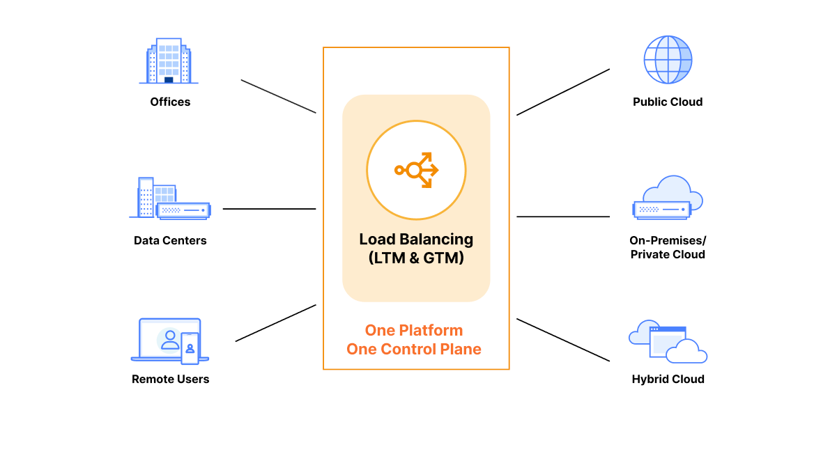
In the dynamic world of modern applications, efficient load balancing plays a pivotal role in delivering exceptional user experiences. Customers commonly leverage load balancing, so they can efficiently use their existing infrastructure resources in the best way possible. Though, load balancing is not a ‘one-size-fits-all, out of the box’ solution for everyone. As you go deeper into the details of your traffic shaping requirements and as your architecture becomes more complex, different flavors of load balancing are usually required to achieve these varying goals, such as steering between datacenters for public traffic, creating high availability for critical internal services with private IPs, applying steering between servers in a single datacenter, and more. We are extremely excited to announce a new addition to our Load Balancing solution, Local Traffic Management (LTM) with deep integrations with Zero Trust!
A common problem businesses run into is that almost no providers can satisfy all these requirements, resulting in a growing list of vendors to manage disparate data sources to get a clear view of your traffic pipeline, and investment into incredibly expensive hardware that is complicated to set up and maintain. Not having a single source of truth to dwindle down ‘time to resolution’ and a single partner to work with in times when things are not operating within the ideal path can be the difference between a proactive, healthy growing business versus one that is reactive and constantly having to put out fires. The latter can result in extreme slowdown to developing amazing features/services, reduction in revenue, tarnishing of brand trust, decreases in adoption – the list goes on!
For eight years, we have provided top-tier global traffic load balancing (GTM) capabilities to thousands of customers across the globe. But why should the steering intelligence, failover, and reliability we guarantee stop at the front door of the selected datacenter and only operate with public traffic? We came to the conclusion that we should go even further. Today is the start of a long series of new features that allow traffic steering, failover, session persistence, SSL/TLS offloading and much more to take place between servers after datacenter selection has occurred! Instead of relying only on the relative weight to determine which server traffic should be sent to, you can now bring the same intelligent steering policies, such as least outstanding requests steering or hash steering, to any of your many data centers. This also means you have a single partner for all of your load balancing initiatives and a single pane of glass to inform business decisions! Cloudflare is thrilled to introduce the powerful combination of private IP support for Load Balancing with Cloudflare Tunnels and Local Traffic Management, offering customers a solution that blends unparalleled efficiency, security, flexibility, and privacy.
What is a load balancer?
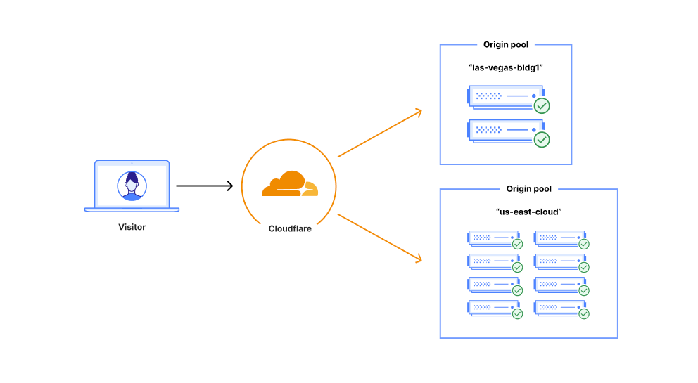
Load balancing — functionality that’s been around for the last 30 years to help businesses leverage their existing infrastructure resources. Load balancing works by proactively steering traffic away from unhealthy origin servers and — for more advanced solutions — intelligently distributing traffic load based on different steering algorithms. This process ensures that errors aren’t served to end users and empowers businesses to tightly couple overall business objectives to their traffic behavior. Cloudflare Load Balancing has made it simpler and easier to securely and reliably manage your traffic across multiple data centers around the world. With Cloudflare Load Balancing, your traffic will be directed reliably regardless of the scale of traffic or where it originates with customizable steering, affinity and failover. This clearly has an advantage over a physical load balancer since it can be configured easily and traffic doesn’t have to reach one of your data centers to be routed to another location, introducing single points of failure and significant latency. When compared with other global traffic management load balancers, Cloudflare’s Load Balancing offering is easier to set up, simpler to understand, and is fully integrated with the Cloudflare platform as one single product for all load balancing needs.
What are Cloudflare Tunnels?
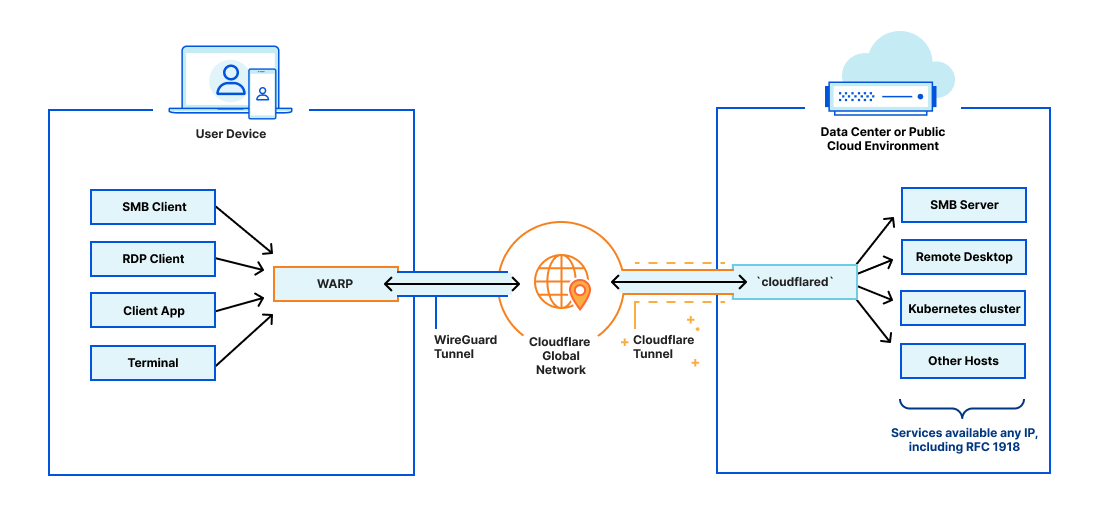
In 2018, Cloudflare introduced Cloudflare Tunnels, a private, secure connection between your data center and Cloudflare. Traditionally, from the moment an Internet property is deployed, developers spend an exhaustive amount of time and energy locking it down through access control lists, rotating IP addresses, or more complex solutions like GRE tunnels. We built Tunnel to help alleviate that burden. With Tunnels, users can create a private link from their origin server directly to Cloudflare without exposing your services directly to the public internet or allowing incoming connections in your data center’s firewall. Instead, this private connection is established by running a lightweight daemon, cloudflared, in your data center, which creates a secure, outbound-only connection. This means that only traffic that you’ve configured to pass through Cloudflare can reach your private origin.
Unleashing the potential of Cloudflare Load Balancing with Cloudflare Tunnels
Combining Cloudflare Tunnels with Cloudflare Load Balancing allows you to remove your physical load balancers from your data center and have your Cloudflare load balancer reach out to your servers directly via their private IP addresses with health checks, steering, and all other Load Balancing features currently available. Instead of configuring your on-premise load balancer to expose each service and then updating your Cloudflare load balancer, you can configure it all in one place. This means that from the end-user to the server handling the request, all your configuration can be done in a single place – the Cloudflare dashboard. On top of this, you can say goodbye to the multi hundred thousand dollar price tag to hardware appliances, the incredible management overhead and investing in a solution that has a time limit for its delivered value.
Load Balancing serves as the backbone for online services, ensuring seamless traffic distribution across servers or data centers. Traditional load balancing techniques often require exposing services on a data center’s public IP addresses, forcing organizations to create complex configurations vulnerable to security risks and potential data exposure. By harnessing the power of private IP support for Load Balancing in conjunction with Cloudflare Tunnels, Cloudflare is revolutionizing the way businesses protect and optimize their applications. With clear steps to install the cloudflared agent to connect your private network to Cloudflare’s network via Cloudflare Tunnels, directly and securely routing traffic into your data centers becomes easier than ever before!
Publicly exposing services in private data centers is complicated
Load balancing within a private data center can be expensive and difficult to manage. The idea of keeping security first while ensuring ease of use and flexibility for your internal workforce is a tricky balance to strike. It’s not only the ‘how’ of securely exposing internal services, but how to best balance traffic between servers at a single location within your private network!
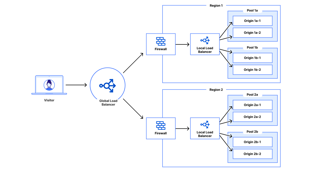
In a private data center, even a very simple website can be fairly complex in terms of networking and configuration. Let’s walk through a simple example of a customer device connecting to a website. A customer device performs a DNS lookup for the business’s website and receives an IP address corresponding to a customer data center. The customer then makes an HTTPS request to that IP address, passing the original hostname via Server Name Indication (SNI). That load balancer forwards that request to the corresponding origin server and returns the response to the customer device.
This example doesn’t have any advanced functionality and the stack is already difficult to configure:
- Expose the service or server on a private IP.
- Configure your data center’s networking to expose the LB on a public IP or IP range.
- Configure your load balancer to forward requests for that hostname and/or public IP to your server’s private IP.
- Configure a DNS record for your domain to point to your load balancer’s public IP.
In large enterprises, each of these configuration changes likely requires approval from several stakeholders and modified through different repositories, websites and/or private web interfaces. Load balancer and networking configurations are often maintained as complex configuration files for Terraform, Chef, Puppet, Ansible or a similar infrastructure-as-code service. These configuration files can be syntax checked or tested but are rarely tested thoroughly prior to deployment. Each deployment environment is often unique enough that thorough testing is often not feasible given the time and hardware requirements needed to do so. This means that changes to these files can negatively affect other services within the data center. In addition, opening up an ingress to your data center widens the attack surface for varying security risks such as DDoS attacks or catastrophic data breaches. To make things worse, each vendor has a different interface or API for configuring their devices or services. For example, some registrars only have XML APIs while others have JSON REST APIs. Each device configuration may have different Terraform providers or Ansible playbooks. This results in complex configurations accumulating over time that are difficult to consolidate or standardize, inevitably resulting in technical debt.
Now let’s add additional origins. For each additional origin for our service, we’ll have to go set up and expose that origin and configure the physical load balancer to use our new origin. Now let’s add another data center. Now we need another solution to distribute across our data centers. This results in a separate global traffic management system and local traffic management system. These solutions have in the past come from different vendors and will have to be configured in different ways even though they should serve the same purpose: load balancing. This makes managing your web traffic unnecessarily difficult. Why should you have to configure your origins in two different load balancers? Why can’t you manage all the traffic for all the origins for a service in the same place?
Simpler and better: Load Balancing with Tunnels
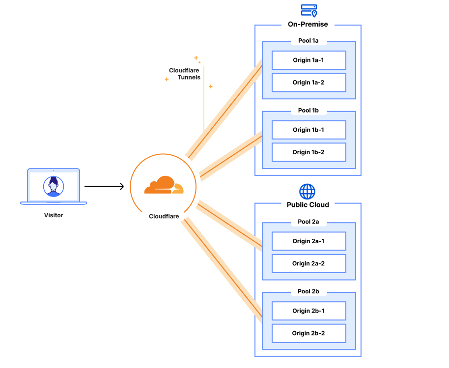
With Cloudflare Load Balancing and Cloudflare Tunnel, you can manage all your public and private origins in one place: the Cloudflare dashboard. Cloudflare load balancers can be easily configured using the Cloudflare dashboard or the Cloudflare API. There’s no need to SSH or open a remote desktop to modify load balancer configurations for your public or private servers. All configurations can be done through the dashboard UI or Cloudflare API, with full parity between the two.
With Cloudflare Tunnel set up and running in your data center, everything is ready to connect your origin server to Cloudflare network and load balancers. You do not need to configure any ingress to your data center since Cloudflare Tunnel operates only over outbound connections and can securely reach out to privately addressed services inside your data center. To expose your service to Cloudflare, you just set up your private IP range to be routed over that tunnel. Then, you can create a Cloudflare load balancer and input the corresponding private IP address and virtual network ID into your origin pool. After that, Cloudflare manages the DNS and load balancing across your private servers. Now your origin is receiving traffic exclusively via Cloudflare Tunnel and your physical load balancer is no longer needed!
This groundbreaking integration enables organizations to deploy load balancers while keeping their applications securely shielded from the public Internet. The customer’s traffic passes through Cloudflare’s data centers, allowing customers to continue to take full advantage of Cloudflare’s security and performance services. Also, by leveraging Cloudflare Tunnels, traffic between Cloudflare and customer origins remains isolated within trusted networks, bolstering privacy, security, and peace of mind.
The advantages of Private IP support with Cloudflare Tunnels
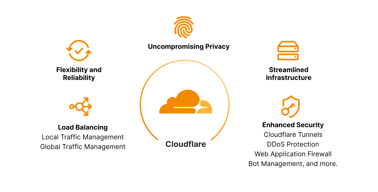
Combining Global and Local Traffic Management: All the features and ease of use that were part of Cloudflare Load Balancing for Global Traffic Management are also available with Local Traffic Management. You can configure your public and private origins in one dashboard as opposed to several services and vendors. Now, all your private origins can benefit from the features that Cloudflare Load Balancing is known for: instant failover, customizable steering between data centers, ease of use, custom rules and configuration updates in a matter of seconds. They will also benefit from our newer features including least connection steering, least outstanding request steering, and session affinity by header. This is just a small subset of the expansive feature set for Load Balancing. See our dev docs for more features and details on the offering.
Enhanced Security: By combining private IP support with Cloudflare Tunnels, organizations can fortify their security posture and protect sensitive data. With private IP addresses and encrypted connections via Cloudflare Tunnel, the risk of unauthorized access and potential attacks is significantly reduced – traffic remains within trusted networks. You can also configure Cloudflare Access to add single sign-on support for your application and restrict your application to a subset of authorized users. In addition, you still benefit from Firewall rules, Rate Limiting rules, Bot Management, DDoS protection and all the other Cloudflare products available today allowing comprehensive security configurations.
Uncompromising Privacy: As data privacy continues to take center stage, businesses must ensure the confidentiality of user information. Cloudflare's private IP support with Cloudflare Tunnels enables organizations to segregate applications and keep sensitive data within their private network boundaries. Custom rules also allow you to direct traffic for specific devices to specific data centers. For example, you can use custom rules to direct traffic from Eastern and Western Europe to your European data centers, so you can easily keep those users’ data within Europe. This minimizes the exposure of data to external entities, preserving user privacy and complying with strict privacy regulations across different geographies.
Flexibility & Reliability: Scale and adaptability are some of the major foundations of a well-operating business. Implementing solutions that fit your business’ needs today is not enough. Customers must find solutions that meet their needs for the next three or more years. The blend of Load Balancing with Cloudflare Tunnels within our Zero Trust solution lends to the very definition of flexibility and reliability! Changes to load balancer configurations propagate around the world in a matter of seconds, making load balancers an effective way to respond to incidents. Also, instant failover, health monitoring, and steering policies all help to maintain high availability for your applications, so you can deliver the reliability that your users expect. This is all in addition to best in class Zero Trust capabilities that are deeply integrated such as, but not limited to Secure Web Gateway (SWG), remote browser isolation, network logs. Data loss prevention.
Streamlined Infrastructure: Organizations can consolidate their network architecture and establish secure connections across distributed environments. This unification reduces complexity, lowers operational overhead, and facilitates efficient resource allocation. Whether you need to apply a global traffic manager to intelligently direct traffic between datacenters within your private network, or steer between specific servers after datacenter selection has taken place, there is now a clear, single lens to manage your global and local traffic, regardless of whether the source or destination of the traffic is public or private. Complexity can be a large hurdle in achieving and maintaining fast, agile business units. Consolidating into a single provider, like Cloudflare, that provides security, reliability, and observability will not only save significant cost but allows your teams to move faster and focus on growing their business, enhancing critical services, and developing incredible features, rather than taping together infrastructure that may not work in a few years. Leave the heavy lifting to us, and let us empower you and your team to focus on creating amazing experiences for your employees and end-users.
The lack of agility, flexibility, and lean operations of hardware appliances for Local Traffic Management does not justify the hundreds of thousands of dollars spent on them, along with the huge overhead of managing CPU, memory, power, cooling, etc. Instead, we want to help businesses move this logic to the cloud by abstracting away the needless overhead and bringing more focus back to teams to do what they do best, building amazing experiences, and allowing Cloudflare to do what we do best, protecting, accelerating, and building heightened reliability. Stay tuned for more updates on Cloudflare's Local Traffic Manager and how it can reduce architecture complexity while bringing more insight, security, and control to your teams. In the meantime, check out our new whitepaper!
Looking to the future
Cloudflare's impactful solution, private IP support for Load Balancing with Cloudflare Tunnels as part of the Zero Trust solution, reaffirms our commitment to providing cutting-edge tools that prioritize security, privacy, and performance. By leveraging private IP addresses and secure tunnels, Cloudflare empowers businesses to fortify their network infrastructure while ensuring compliance with regulatory requirements. With enhanced security, uncompromising privacy, and streamlined infrastructure, load balancing becomes a powerful driver of efficient and secure public or private services.
As a business grows and its systems scale up, they'll need the features that Cloudflare Load Balancing is known for: health monitoring, steering, and failover. As availability requirements increase due to growing demands and standards from end-users, customers can add health checks, enabling automatic failover to healthy servers when an unhealthy server begins to fail. When the business begins to receive more traffic from around the world, they can create new pools for different regions and use dynamic steering to reduce latency between the user and the server. For intensive or long-running requests, such as complex datastore queries, customers can benefit from leveraging least outstanding requests steering to reduce the number of concurrent requests per server. Before, this could all be done with publicly addressable IPs, but it is now available for pools with public IPs, private servers, or combinations of the two. Private IP Load Balancing along with Local Traffic Management is live and ready to use today! Check out our dev docs for instructions on how to get started.
Stay tuned for our next addition to add new Load Balancing onramp support for Spectrum and WARP with Cloudflare Tunnels with private IPs for your Layer 4 traffic, allowing us to support TCP and UDP applications in your private data centers!
The Rise and Fall of the American Mall
Post Syndicated from The History Guy: History Deserves to Be Remembered original https://www.youtube.com/watch?v=Ex3n8hyEzNs
LLMs and Tool Use
Post Syndicated from Bruce Schneier original https://www.schneier.com/blog/archives/2023/09/ai-tool-use.html
Last March, just two weeks after GPT-4 was released, researchers at Microsoft quietly announced a plan to compile millions of APIs—tools that can do everything from ordering a pizza to solving physics equations to controlling the TV in your living room—into a compendium that would be made accessible to large language models (LLMs). This was just one milestone in the race across industry and academia to find the best ways to teach LLMs how to manipulate tools, which would supercharge the potential of AI more than any of the impressive advancements we’ve seen to date.
The Microsoft project aims to teach AI how to use any and all digital tools in one fell swoop, a clever and efficient approach. Today, LLMs can do a pretty good job of recommending pizza toppings to you if you describe your dietary preferences and can draft dialog that you could use when you call the restaurant. But most AI tools can’t place the order, not even online. In contrast, Google’s seven-year-old Assistant tool can synthesize a voice on the telephone and fill out an online order form, but it can’t pick a restaurant or guess your order. By combining these capabilities, though, a tool-using AI could do it all. An LLM with access to your past conversations and tools like calorie calculators, a restaurant menu database, and your digital payment wallet could feasibly judge that you are trying to lose weight and want a low-calorie option, find the nearest restaurant with toppings you like, and place the delivery order. If it has access to your payment history, it could even guess at how generously you usually tip. If it has access to the sensors on your smartwatch or fitness tracker, it might be able to sense when your blood sugar is low and order the pie before you even realize you’re hungry.
Perhaps the most compelling potential applications of tool use are those that give AIs the ability to improve themselves. Suppose, for example, you asked a chatbot for help interpreting some facet of ancient Roman law that no one had thought to include examples of in the model’s original training. An LLM empowered to search academic databases and trigger its own training process could fine-tune its understanding of Roman law before answering. Access to specialized tools could even help a model like this better explain itself. While LLMs like GPT-4 already do a fairly good job of explaining their reasoning when asked, these explanations emerge from a “black box” and are vulnerable to errors and hallucinations. But a tool-using LLM could dissect its own internals, offering empirical assessments of its own reasoning and deterministic explanations of why it produced the answer it did.
If given access to tools for soliciting human feedback, a tool-using LLM could even generate specialized knowledge that isn’t yet captured on the web. It could post a question to Reddit or Quora or delegate a task to a human on Amazon’s Mechanical Turk. It could even seek out data about human preferences by doing survey research, either to provide an answer directly to you or to fine-tune its own training to be able to better answer questions in the future. Over time, tool-using AIs might start to look a lot like tool-using humans. An LLM can generate code much faster than any human programmer, so it can manipulate the systems and services of your computer with ease. It could also use your computer’s keyboard and cursor the way a person would, allowing it to use any program you do. And it could improve its own capabilities, using tools to ask questions, conduct research, and write code to incorporate into itself.
It’s easy to see how this kind of tool use comes with tremendous risks. Imagine an LLM being able to find someone’s phone number, call them and surreptitiously record their voice, guess what bank they use based on the largest providers in their area, impersonate them on a phone call with customer service to reset their password, and liquidate their account to make a donation to a political party. Each of these tasks invokes a simple tool—an Internet search, a voice synthesizer, a bank app—and the LLM scripts the sequence of actions using the tools.
We don’t yet know how successful any of these attempts will be. As remarkably fluent as LLMs are, they weren’t built specifically for the purpose of operating tools, and it remains to be seen how their early successes in tool use will translate to future use cases like the ones described here. As such, giving the current generative AI sudden access to millions of APIs—as Microsoft plans to—could be a little like letting a toddler loose in a weapons depot.
Companies like Microsoft should be particularly careful about granting AIs access to certain combinations of tools. Access to tools to look up information, make specialized calculations, and examine real-world sensors all carry a modicum of risk. The ability to transmit messages beyond the immediate user of the tool or to use APIs that manipulate physical objects like locks or machines carries much larger risks. Combining these categories of tools amplifies the risks of each.
The operators of the most advanced LLMs, such as OpenAI, should continue to proceed cautiously as they begin enabling tool use and should restrict uses of their products in sensitive domains such as politics, health care, banking, and defense. But it seems clear that these industry leaders have already largely lost their moat around LLM technology—open source is catching up. Recognizing this trend, Meta has taken an “If you can’t beat ’em, join ’em” approach and partially embraced the role of providing open source LLM platforms.
On the policy front, national—and regional—AI prescriptions seem futile. Europe is the only significant jurisdiction that has made meaningful progress on regulating the responsible use of AI, but it’s not entirely clear how regulators will enforce it. And the US is playing catch-up and seems destined to be much more permissive in allowing even risks deemed “unacceptable” by the EU. Meanwhile, no government has invested in a “public option” AI model that would offer an alternative to Big Tech that is more responsive and accountable to its citizens.
Regulators should consider what AIs are allowed to do autonomously, like whether they can be assigned property ownership or register a business. Perhaps more sensitive transactions should require a verified human in the loop, even at the cost of some added friction. Our legal system may be imperfect, but we largely know how to hold humans accountable for misdeeds; the trick is not to let them shunt their responsibilities to artificial third parties. We should continue pursuing AI-specific regulatory solutions while also recognizing that they are not sufficient on their own.
We must also prepare for the benign ways that tool-using AI might impact society. In the best-case scenario, such an LLM may rapidly accelerate a field like drug discovery, and the patent office and FDA should prepare for a dramatic increase in the number of legitimate drug candidates. We should reshape how we interact with our governments to take advantage of AI tools that give us all dramatically more potential to have our voices heard. And we should make sure that the economic benefits of superintelligent, labor-saving AI are equitably distributed.
We can debate whether LLMs are truly intelligent or conscious, or have agency, but AIs will become increasingly capable tool users either way. Some things are greater than the sum of their parts. An AI with the ability to manipulate and interact with even simple tools will become vastly more powerful than the tools themselves. Let’s be sure we’re ready for them.
This essay was written with Nathan Sanders, and previously appeared on Wired.com.
Comic for 2023.09.08 – Get Packed
Post Syndicated from Explosm.net original https://explosm.net/comics/get-packed
New Cyanide and Happiness Comic
Gold
Post Syndicated from xkcd.com original https://xkcd.com/2826/

New – Amazon EC2 R7iz Instances Memory-Optimized for High CPU Performance, Memory-Intensive Workloads
Post Syndicated from Veliswa Boya original https://aws.amazon.com/blogs/aws/new-amazon-ec2-r7iz-instances-memory-optimized-for-high-cpu-performance-memory-intensive-workloads/
Today we’re announcing general availability of the Amazon EC2 R7iz instances. R7iz instances are the fastest 4th Generation Intel Xeon Scalable-based (Sapphire Rapids) instances in the cloud with 3.9 GHz sustained all-core turbo frequency. R7iz instances are suitable for workloads where there’s a requirement for more memory to process additional data, larger sizes of instances to scale up, higher compute and memory performance to reduce completion times, and higher networking and Amazon Elastic Block Store (Amazon EBS) performance to improve latency. The high compute performance of the R7iz instances, combined with a large amount of memory, results in increased overall performance for applications that include front-end electronic design automation (EDA), relational database workloads with high per core licensing fees, and financial, actuarial, and data analytics simulation workloads. This can help you speed time to market for product development while reducing licensing costs.
R7iz Instances
The specs for the R7iz instances are as follows.
| vCPUs |
Memory (GiB) |
Network Bandwidth |
EBS Bandwidth |
|
| r7iz.large | 2 | 16 | Up to 12.5 Gbps | Up to 10 Gbps |
| r7iz.xlarge | 4 | 32 | Up to 12.5 Gbps | Up to 10 Gbps |
| r7iz.2xlarge | 8 | 64 | Up to 12.5 Gbps | Up to 10 Gbps |
| r7iz.4xlarge | 16 | 128 | Up to 12.5 Gbps | Up to 10 Gbps |
| r7iz.8xlarge | 32 | 256 | 12.5 Gbps | 10 Gbps |
| r7iz.12xlarge | 48 | 384 | 25 Gbps | 19 Gbps |
| r7iz.16xlarge | 64 | 512 | 25 Gbps | 20 Gbps |
| r7iz.32xlarge | 128 | 1024 | 50 Gbps | 40 Gbps |
You can attach up to 88 EBS volumes to each R7iz instance; by way of comparison, the z1d instances allow you to attach up to 28 volumes.
We are also getting ready to launch two sizes of bare metal R7iz instances:
| vCPUs |
Memory (GiB) |
Network Bandwidth |
EBS Bandwidth |
|
| r7iz.metal-16xl | 64 | 512 | 25 Gbps | 20 Gbps |
| r7iz.metal-32xl | 128 | 1024 | 50 Gbps | 40 Gbps |
Built-in Accelerators
R7iz instances also include four built-in accelerators: Advanced Matrix Extensions (AMX), Intel Data Streaming accelerator (DSA), Intel In-Memory Analytics Accelerator (IAA), and Intel QuickAssist Technology( QAT). Some of these accelerators require the use of specific kernel versions, drivers, and/or compilers. The Advanced Matrix Extensions are available on all sizes of R7iz instances while the Intel QAT, Intel IAA, and Intel DSA accelerators will be available on the r7iz.metal-16xl and r7iz.metal-32xl instances (coming soon).
Available Now
R7iz instances are generally available today in the US East (N. Virginia), and US West (Oregon) AWS Regions. As usual with Amazon EC2, you pay only for what you use. For more information, see Amazon EC2 pricing.
To learn more, visit our Amazon EC2 R7iz instances page, and please send feedback to AWS re:Post for EC2 or through your usual AWS Support contacts.
– Veliswa
Automatically detect and block low-volume network floods
Post Syndicated from Bryan Van Hook original https://aws.amazon.com/blogs/security/automatically-detect-and-block-low-volume-network-floods/
In this blog post, I show you how to deploy a solution that uses AWS Lambda to automatically manage the lifecycle of Amazon VPC Network Access Control List (ACL) rules to mitigate network floods detected using Amazon CloudWatch Logs Insights and Amazon Timestream.
Application teams should consider the impact unexpected traffic floods can have on an application’s availability. Internet-facing applications can be susceptible to traffic that some distributed denial of service (DDoS) mitigation systems can’t detect. For example, hit-and-run events are a popular approach that use short-lived floods that reoccur at random intervals. Each burst is small enough to go unnoticed by mitigation systems, but still occur often enough and are large enough to be disruptive. Automatically detecting and blocking temporary sources of invalid traffic, combined with other best practices, can strengthen the resiliency of your applications and maintain customer trust.
Use resilient architectures
AWS customers can use prescriptive guidance to improve DDoS resiliency by reviewing the AWS Best Practices for DDoS Resiliency. It describes a DDoS-resilient reference architecture as a guide to help you protect your application’s availability.
The best practices above address the needs of most AWS customers; however, in this blog we cover a few outlier examples that fall outside normal guidance. Here are a few examples that might describe your situation:
- You need to operate functionality that isn’t yet fully supported by an AWS managed service that takes on the responsibility of DDoS mitigation.
- Migrating to an AWS managed service such as Amazon Route 53 isn’t immediately possible and you need an interim solution that mitigates risks.
- Network ingress must be allowed from a wide public IP space that can’t be restricted.
- You’re using public IP addresses assigned from the Amazon pool of public IPv4 addresses (which can’t be protected by AWS Shield) rather than Elastic IP addresses.
- The application’s technology stack has limited or no support for horizontal scaling to absorb traffic floods.
- Your HTTP workload sits behind a Network Load Balancer and can’t be protected by AWS WAF.
- Network floods are disruptive but not significant enough (too infrequent or too low volume) to be detected by your managed DDoS mitigation systems.
For these situations, VPC network ACLs can be used to deny invalid traffic. Normally, the limit on rules per network ACL makes them unsuitable for handling truly distributed network floods. However, they can be effective at mitigating network floods that aren’t distributed enough or large enough to be detected by DDoS mitigation systems.
Given the dynamic nature of network traffic and the limited size of network ACLs, it helps to automate the lifecycle of network ACL rules. In the following sections, I show you a solution that uses network ACL rules to automatically detect and block infrastructure layer traffic within 2–5 minutes and automatically removes the rules when they’re no longer needed.
Detecting anomalies in network traffic
You need a way to block disruptive traffic while not impacting legitimate traffic. Anomaly detection can isolate the right traffic to block. Every workload is unique, so you need a way to automatically detect anomalies in the workload’s traffic pattern. You can determine what is normal (a baseline) and then detect statistical anomalies that deviate from the baseline. This baseline can change over time, so it needs to be calculated based on a rolling window of recent activity.
Z-scores are a common way to detect anomalies in time-series data. The process for creating a Z-score is to first calculate the average and standard deviation (a measure of how much the values are spread out) across all values over a span of time. Then for each value in the time window calculate the Z-score as follows:
Z-score = (value – average) / standard deviation
A Z-score exceeding 3.0 indicates the value is an outlier that is greater than 99.7 percent of all other values.
To calculate the Z-score for detecting network anomalies, you need to establish a time series for network traffic. This solution uses VPC flow logs to capture information about the IP traffic in your VPC. Each VPC flow log record provides a packet count that’s aggregated over a time interval. Each flow log record aggregates the number of packets over an interval of 60 seconds or less. There isn’t a consistent time boundary for each log record. This means raw flow log records aren’t a predictable way to build a time series. To address this, the solution processes flow logs into packet bins for time series values. A packet bin is the number of packets sent by a unique source IP address within a specific time window. A source IP address is considered an anomaly if any of its packet bins over the past hour exceed the Z-score threshold (default is 3.0).
When overall traffic levels are low, there might be source IP addresses with a high Z-score that aren’t a risk. To mitigate against false positives, source IP addresses are only considered to be an anomaly if the packet bin exceeds a minimum threshold (default is 12,000 packets).
Let’s review the overall solution architecture.
Solution overview
This solution, shown in Figure 1, uses VPC flow logs to capture information about the traffic reaching the network interfaces in your public subnets. CloudWatch Logs Insights queries are used to summarize the most recent IP traffic into packet bins that are stored in Timestream. The time series table is queried to identify source IP addresses responsible for traffic that meets the anomaly threshold. Anomalous source IP addresses are published to an Amazon Simple Notification Service (Amazon SNS) topic. A Lambda function receives the SNS message and decides how to update the network ACL.
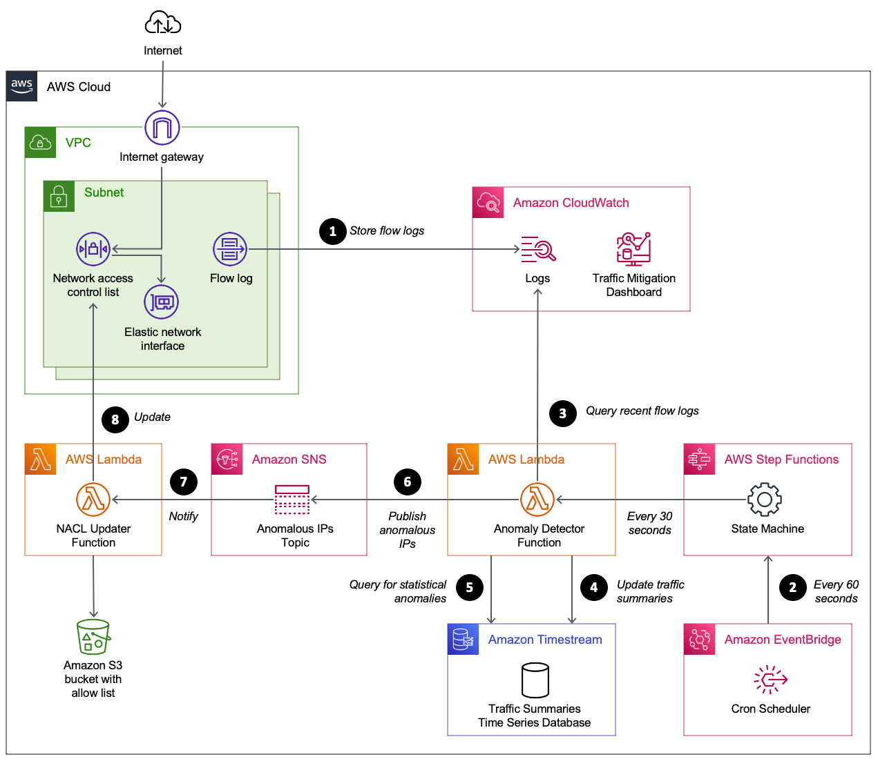
Figure 1: Automating the detection and mitigation of traffic floods using network ACLs
How it works
The numbered steps that follow correspond to the numbers in Figure 1.
- Capture VPC flow logs. Your VPC is configured to stream flow logs to CloudWatch Logs. To minimize cost, the flow logs are limited to particular subnets and only include log fields required by the CloudWatch query. When protecting an endpoint that spans multiple subnets (such as a Network Load Balancer using multiple availability zones), each subnet shares the same network ACL and is configured with a flow log that shares the same CloudWatch log group.
- Scheduled flow log analysis. Amazon EventBridge starts an AWS Step Functions state machine on a time interval (60 seconds by default). The state machine starts a Lambda function immediately, and then again after 30 seconds. The Lambda function performs steps 3–6.
- Summarize recent network traffic. The Lambda function runs a CloudWatch Logs Insights query. The query scans the most recent flow logs (5-minute window) to summarize packet frequency grouped by source IP. These groupings are called packet bins, where each bin represents the number of packets sent by a source IP within a given minute of time.
- Update time series database. A time series database in Timestream is updated with the most recent packet bins.
- Use statistical analysis to detect abusive source IPs. A Timestream query is used to perform several calculations. The query calculates the average bin size over the past hour, along with the standard deviation. These two values are then used to calculate the maximum Z-score for all source IPs over the past hour. This means an abusive IP will remain flagged for one hour even if it stopped sending traffic. Z-scores are sorted so that the most abusive source IPs are prioritized. If a source IP meets these two criteria, it is considered abusive.
- Maximum Z-score exceeds a threshold (defaults to 3.0).
- Packet bin exceeds a threshold (defaults to 12,000). This avoids flagging source IPs during periods of overall low traffic when there is no need to block traffic.
- Publish anomalous source IPs. Publish a message to an Amazon SNS topic with a list of anomalous source IPs. The function also publishes CloudWatch metrics to help you track the number of unique and abusive source IPs over time. At this point, the flow log summarizer function has finished its job until the next time it’s invoked from EventBridge.
- Receive anomalous source IPs. The network ACL updater function is subscribed to the SNS topic. It receives the list of anomalous source IPs.
- Update the network ACL. The network ACL updater function uses two network ACLs called blue and green. This verifies that the active rules remain in place while updating the rules in the inactive network ACL. When the inactive network ACL rules are updated, the function swaps network ACLs on each subnet. By default, each network ACL has a limit of 20 rules. If the number of anomalous source IPs exceeds the network ACL limit, the source IPs with the highest Z-score are prioritized. CloudWatch metrics are provided to help you track the number of source IPs blocked, and how many source IPs couldn’t be blocked due to network ACL limits.
Prerequisites
This solution assumes you have one or more public subnets used to operate an internet-facing endpoint.
Deploy the solution
Follow these steps to deploy and validate the solution.
- Download the latest release from GitHub.
- Upload the AWS CloudFormation templates and Python code to an S3 bucket.
- Gather the information needed for the CloudFormation template parameters.
- Create the CloudFormation stack.
- Monitor traffic mitigation activity using the CloudWatch dashboard.
Let’s review the steps I followed in my environment.
Step 1. Download the latest release
I create a new directory on my computer named auto-nacl-deploy. I review the releases on GitHub and choose the latest version. I download auto-nacl.zip into the auto-nacl-deploy directory. Now it’s time to stage this code in Amazon Simple Storage Service (Amazon S3).
Figure 2: Save auto-nacl.zip to the auto-nacl-deploy directory
Step 2. Upload the CloudFormation templates and Python code to an S3 bucket
I extract the auto-nacl.zip file into my auto-nacl-deploy directory.
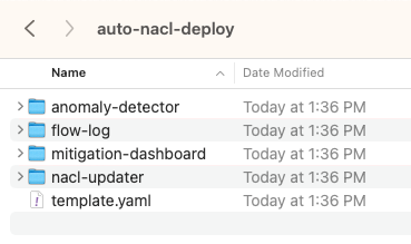
Figure 3: Expand auto-nacl.zip into the auto-nacl-deploy directory
The template.yaml file is used to create a CloudFormation stack with four nested stacks. You copy all files to an S3 bucket prior to creating the stacks.
To stage these files in Amazon S3, use an existing bucket or create a new one. For this example, I used an existing S3 bucket named auto-nacl-us-east-1. Using the Amazon S3 console, I created a folder named artifacts and then uploaded the extracted files to it. My bucket now looks like Figure 4.
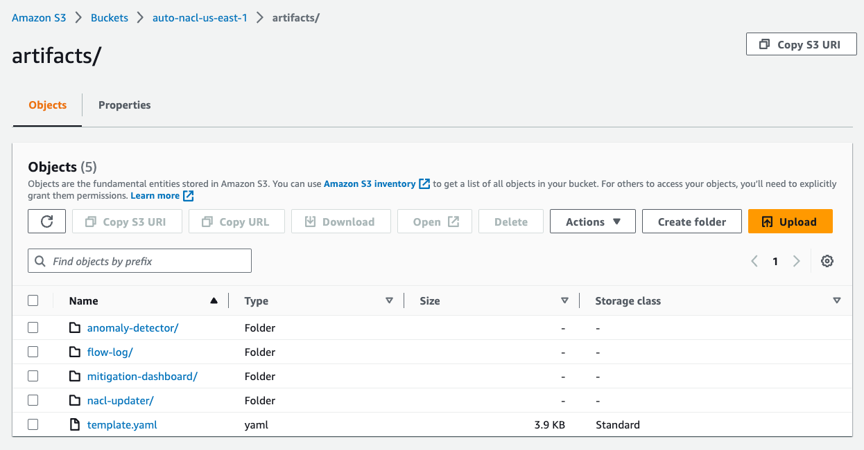
Figure 4: Upload the extracted files to Amazon S3
Step 3. Gather information needed for the CloudFormation template parameters
There are six parameters required by the CloudFormation template.
| Template parameter | Parameter description |
| VpcId | The ID of the VPC that runs your application. |
| SubnetIds | A comma-delimited list of public subnet IDs used by your endpoint. |
| ListenerPort | The IP port number for your endpoint’s listener. |
| ListenerProtocol | The Internet Protocol (TCP or UDP) used by your endpoint. |
| SourceCodeS3Bucket | The S3 bucket that contains the files you uploaded in Step 2. This bucket must be in the same AWS Region as the CloudFormation stack. |
| SourceCodeS3Prefix | The S3 prefix (folder) of the files you uploaded in Step 2. |
For the VpcId parameter, I use the VPC console to find the VPC ID for my application.
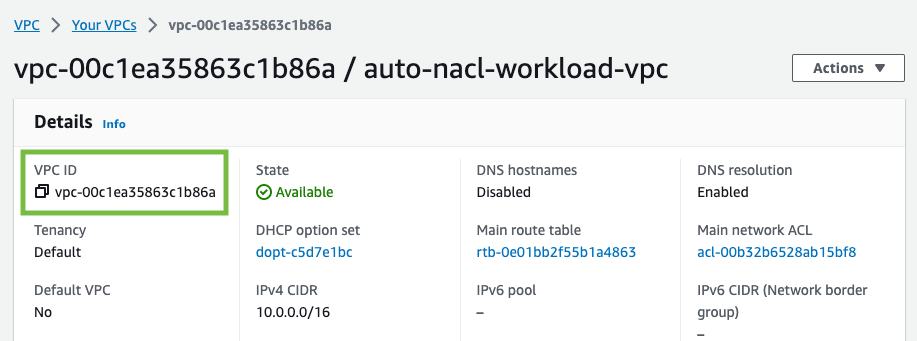
Figure 5: Find the VPC ID
For the SubnetIds parameter, I use the VPC console to find the subnet IDs for my application. My VPC has public and private subnets. For this solution, you only need the public subnets.
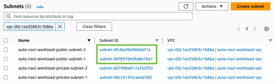
Figure 6: Find the subnet IDs
My application uses a Network Load Balancer that listens on port 80 to handle TCP traffic. I use 80 for ListenerPort and TCP for ListenerProtocol.
The next two parameters are based on the Amazon S3 location I used earlier. I use auto-nacl-us-east-1 for SourceCodeS3Bucket and artifacts for SourceCodeS3Prefix.
Step 4. Create the CloudFormation stack
I use the CloudFormation console to create a stack. The Amazon S3 URL format is https://<bucket>.s3.<region>.amazonaws.com/<prefix>/template.yaml. I enter the Amazon S3 URL for my environment, then choose Next.
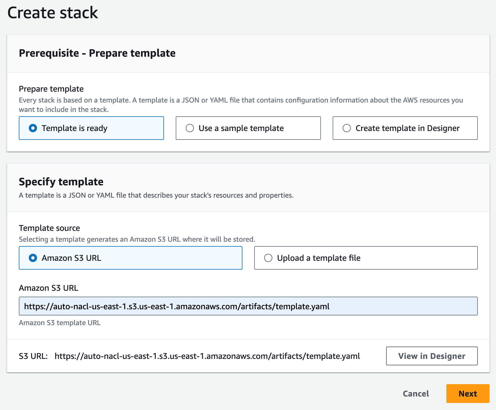
Figure 7: Specify the CloudFormation template
I enter a name for my stack (for example, auto-nacl-1) along with the parameter values I gathered in Step 3. I leave all optional parameters as they are, then choose Next.
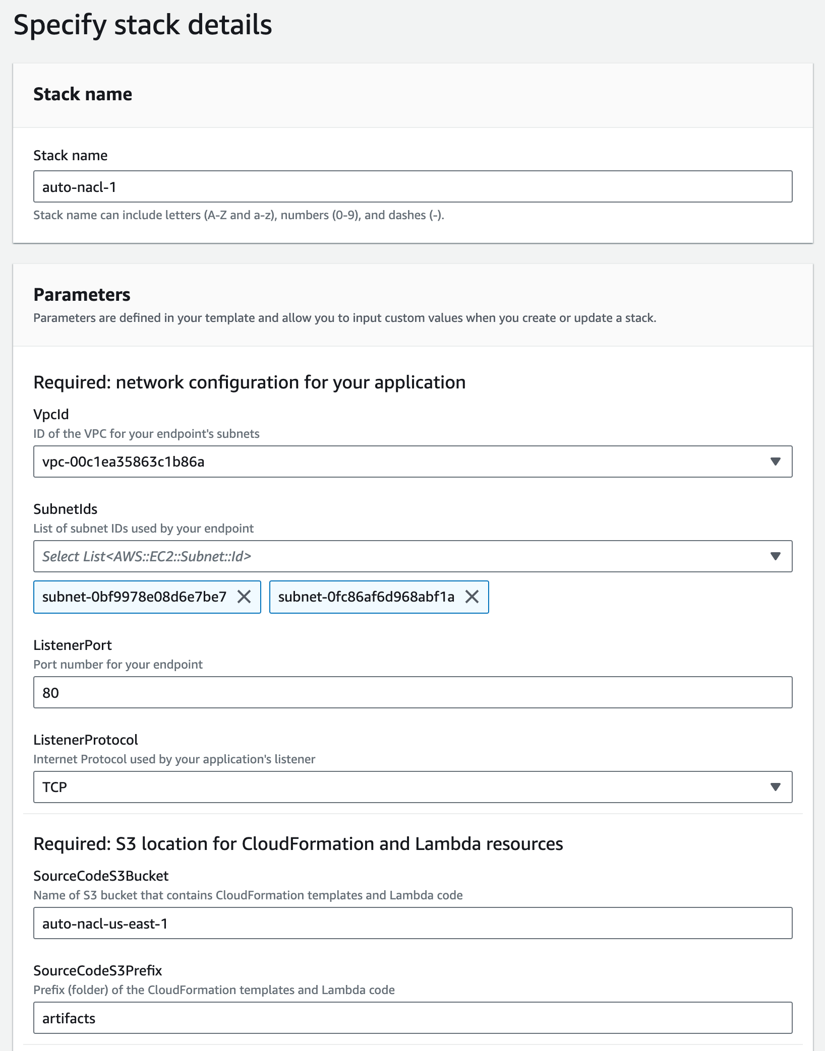
Figure 8: Provide the required parameters
I review the stack options, then scroll to the bottom and choose Next.
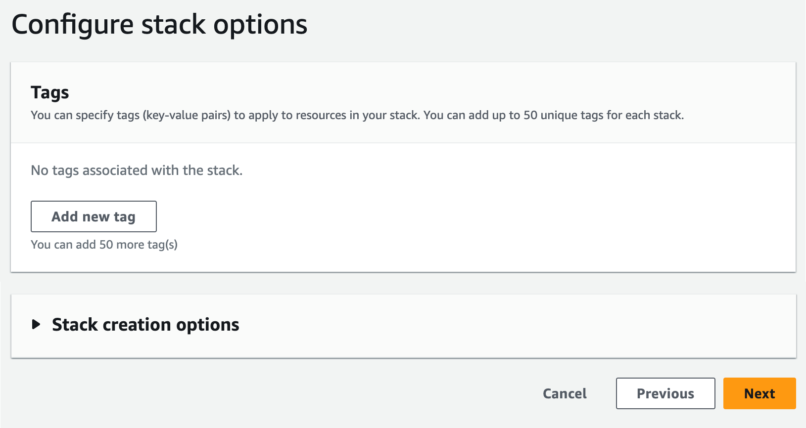
Figure 9: Review the default stack options
I scroll down to the Capabilities section and acknowledge the capabilities required by CloudFormation, then choose Submit.
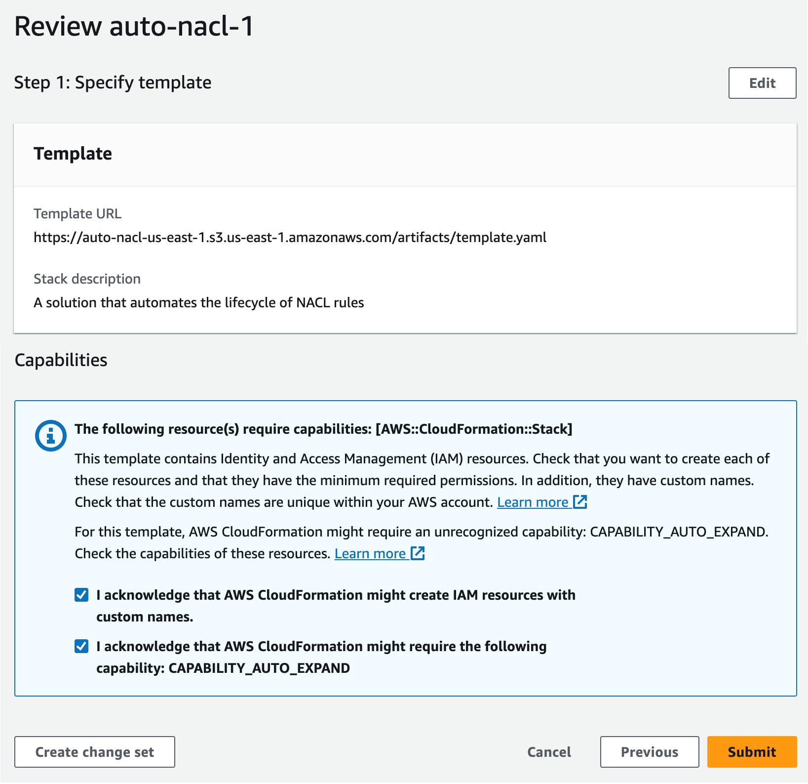
Figure 10: Acknowledge the capabilities required by CloudFormation
I wait for the stack to reach CREATE_COMPLETE status. It takes 10–15 minutes to create all of the nested stacks.
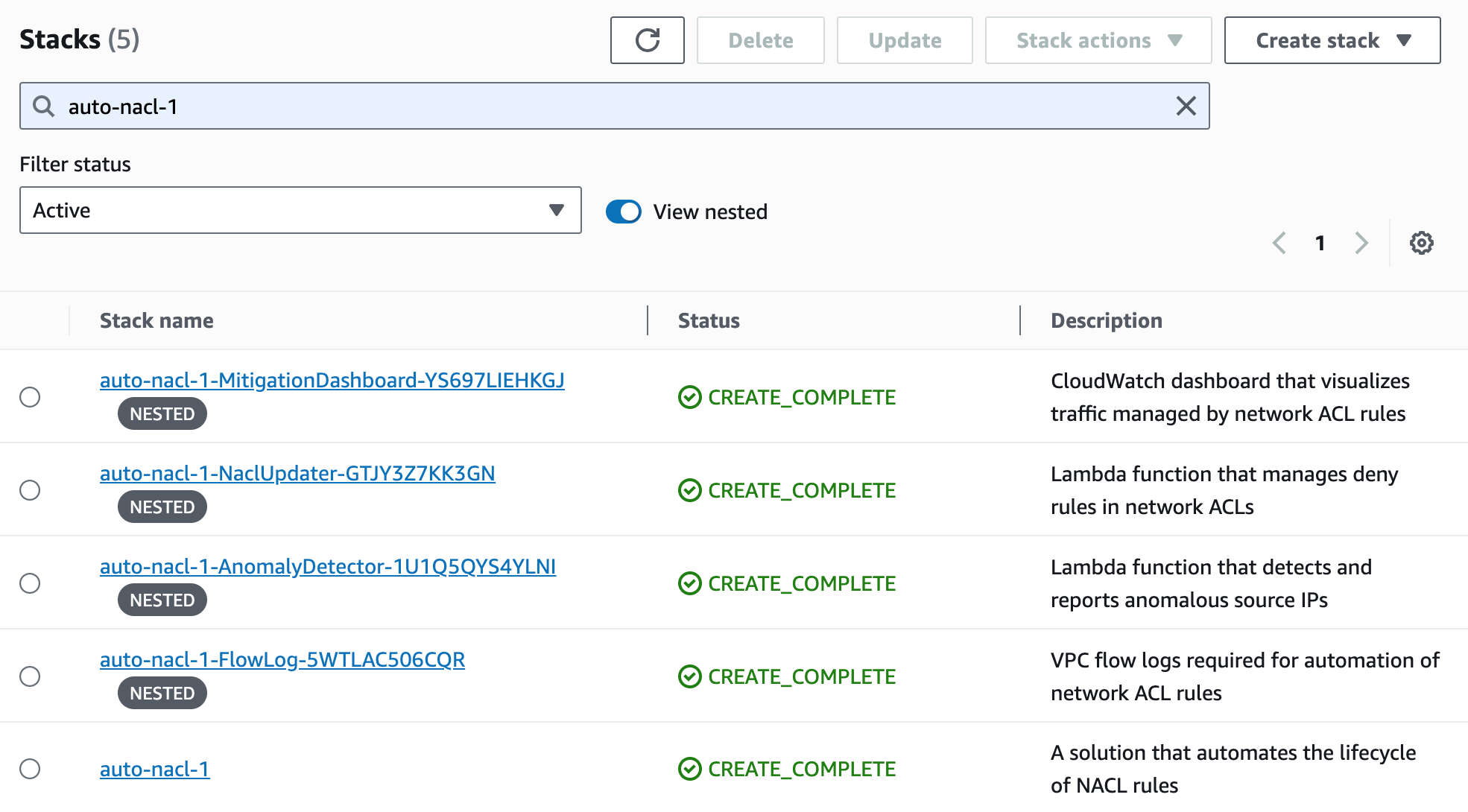
Figure 11: Wait for the stacks to complete
Step 5. Monitor traffic mitigation activity using the CloudWatch dashboard
After the CloudFormation stacks are complete, I navigate to the CloudWatch console to open the dashboard. In my environment, the dashboard is named auto-nacl-1-MitigationDashboard-YS697LIEHKGJ.
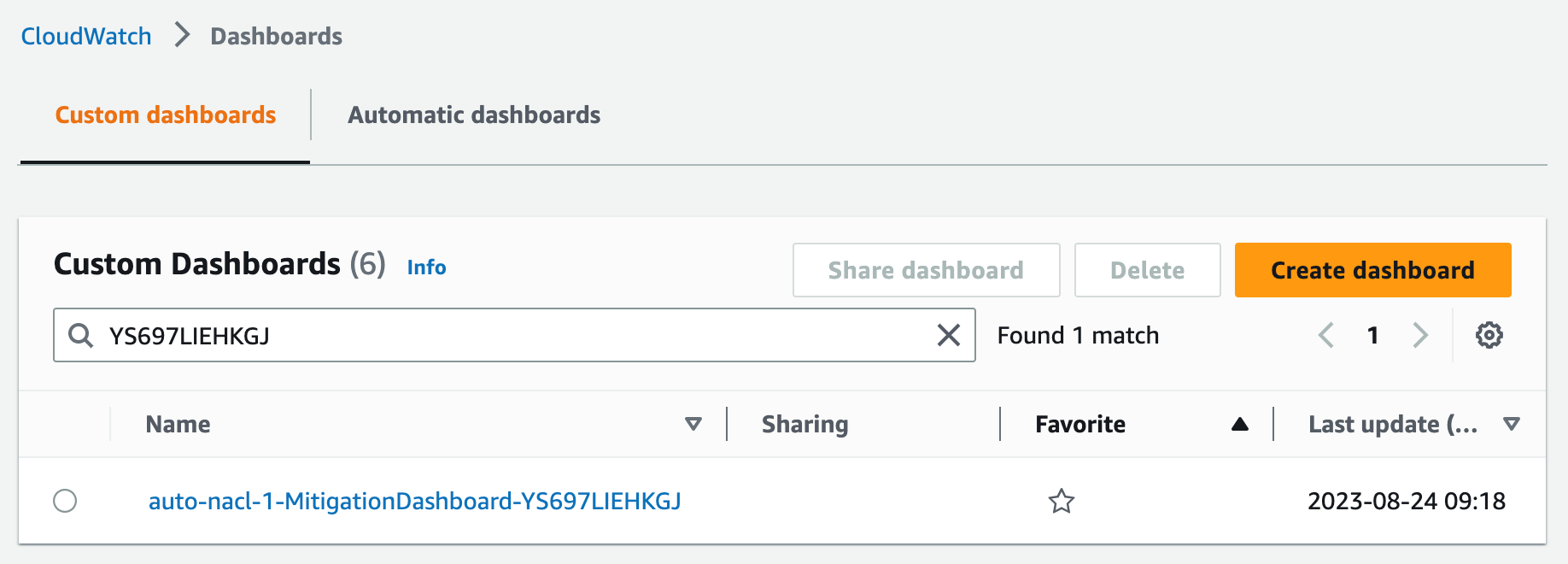
Figure 12: Find the CloudWatch dashboard
Initially, the dashboard, shown in Figure 13, has little information to display. After an hour, I can see the following metrics from my sample environment:
- The Network Traffic graph shows how many packets are allowed and rejected by network ACL rules. No anomalies have been detected yet, so this only shows allowed traffic.
- The All Source IPs graph shows how many total unique source IP addresses are sending traffic.
- The Anomalous Source Networks graph shows how many anomalous source networks are being blocked by network ACL rules (or not blocked due to network ACL rule limit). This graph is blank unless anomalies have been detected in the last hour.
- The Anomalous Source IPs graph shows how many anomalous source IP addresses are being blocked (or not blocked) by network ACL rules. This graph is blank unless anomalies have been detected in the last hour.
- The Packet Statistics graph can help you determine if the sensitivity should be adjusted. This graph shows the average packets-per-minute and the associated standard deviation over the past hour. It also shows the anomaly threshold, which represents the minimum number of packets-per-minute for a source IP address to be considered an anomaly. The anomaly threshold is calculated based on the CloudFormation parameter MinZScore.
anomaly threshold = (MinZScore * standard deviation) + average
Increasing the MinZScore parameter raises the threshold and reduces sensitivity. You can also adjust the CloudFormation parameter MinPacketsPerBin to mitigate against blocking traffic during periods of low volume, even if a source IP address exceeds the minimum Z-score.
- The Blocked IPs grid shows which source IP addresses are being blocked during each hour, along with the corresponding packet bin size and Z-score. This grid is blank unless anomalies have been detected in the last hour.
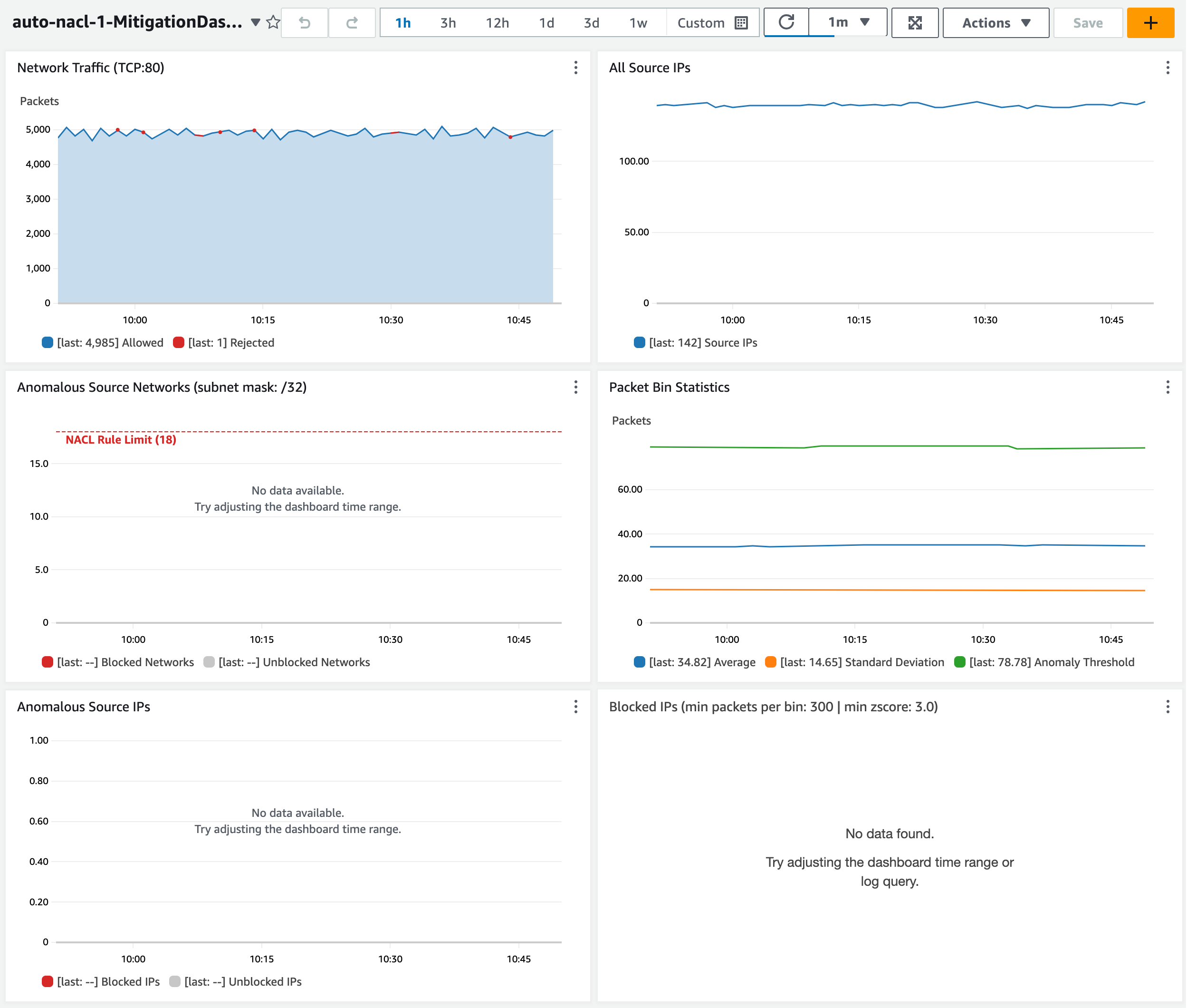
Figure 13: Observe the dashboard after one hour
Let’s review a scenario to see what happens when my endpoint sees two waves of anomalous traffic.
By default, my network ACL allows a maximum of 20 inbound rules. The two default rules count toward this limit, so I only have room for 18 more inbound rules. My application sees a spike of network traffic from 20 unique source IP addresses. When the traffic spike begins, the anomaly is detected in less than five minutes. Network ACL rules are created to block the top 18 source IP addresses (sorted by Z-score). Traffic is blocked for about 5 minutes until the flood subsides. The rules remain in place for 1 hour by default. When the same 20 source IP addresses send another traffic flood a few minutes later, most traffic is immediately blocked. Some traffic is still allowed from two source IP addresses that can’t be blocked due to the limit of 18 rules.
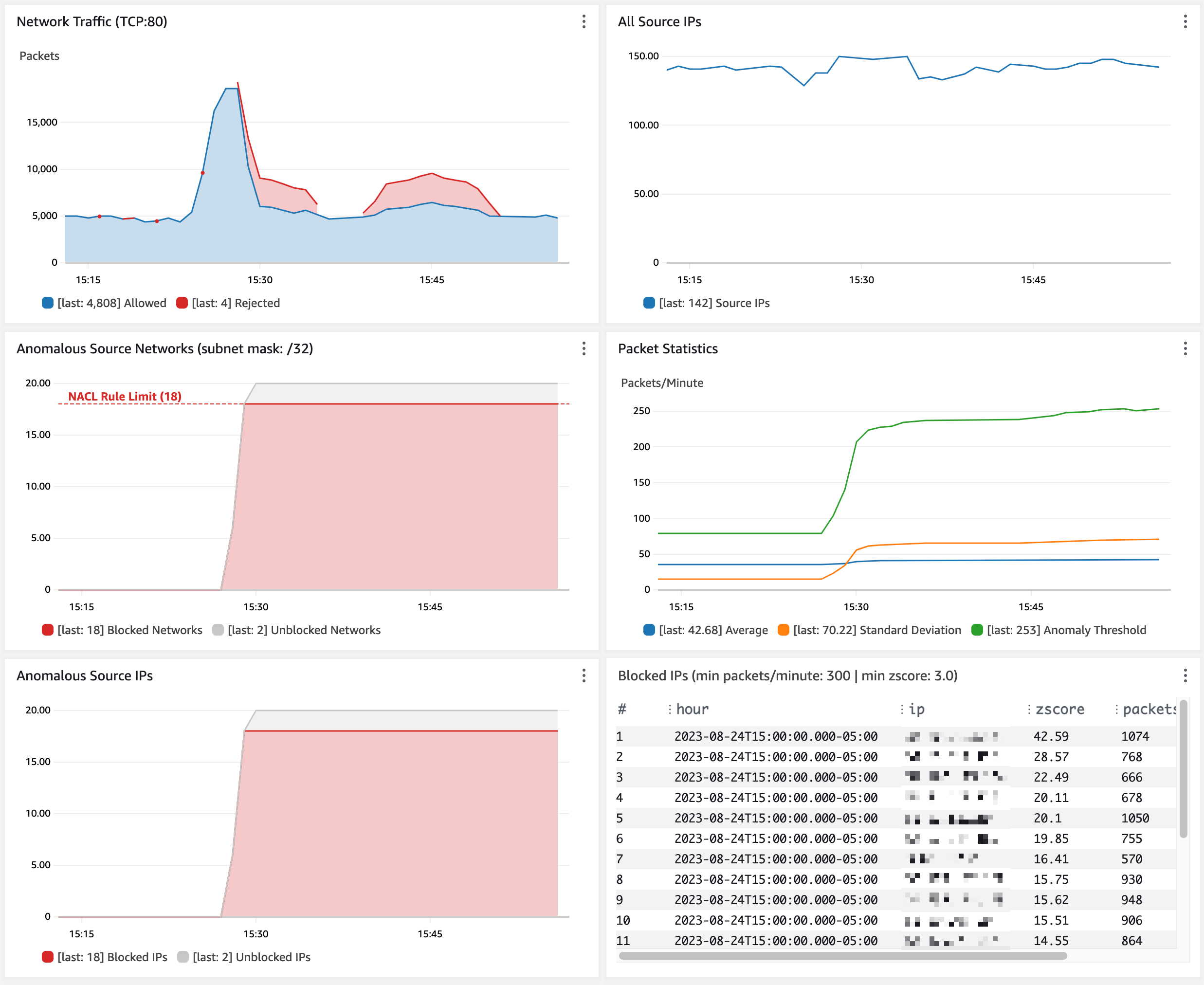
Figure 14: Observe traffic blocked from anomalous source IP addresses
Customize the solution
You can customize the behavior of this solution to fit your use case.
- Block many IP addresses per network ACL rule. To enable blocking more source IP addresses than your network ACL rule limit, change the CloudFormation parameter NaclRuleNetworkMask (default is 32). This sets the network mask used in network ACL rules and lets you block IP address ranges instead of individual IP addresses. By default, the IP address 192.0.2.1 is blocked by a network ACL rule for 192.0.2.1/32. Setting this parameter to 24 results in a network ACL rule that blocks 192.0.2.0/24. As a reminder, address ranges that are too wide might result in blocking legitimate traffic.
- Only block source IPs that exceed a packet volume threshold. Use the CloudFormation parameter MinPacketsPerBin (default is 12,000) to set the minimum packets per minute. This mitigates against blocking source IPs (even if their Z-score is high) during periods of overall low traffic when there is no need to block traffic.
- Adjust the sensitivity of anomaly detection. Use the CloudFormation parameter MinZScore to set the minimum Z-score for a source IP to be considered an anomaly. The default is 3.0, which only blocks source IPs with packet volume that exceeds 99.7 percent of all other source IPs.
- Exclude trusted source IPs from anomaly detection. Specify an allow list object in Amazon S3 that contains a list of IP addresses or CIDRs that you want to exclude from network ACL rules. The network ACL updater function reads the allow list every time it handles an SNS message.
Limitations
As covered in the preceding sections, this solution has a few limitations to be aware of:
- CloudWatch Logs queries can only return up to 10,000 records. This means the traffic baseline can only be calculated based on the observation of 10,000 unique source IP addresses per minute.
- The traffic baseline is based on a rolling 1-hour window. You might need to increase this if a 1-hour window results in a baseline that allows false positives. For example, you might need a longer baseline window if your service normally handles abrupt spikes that occur hourly or daily.
- By default, a network ACL can only hold 20 inbound rules. This includes the default allow and deny rules, so there’s room for 18 deny rules. You can increase this limit from 20 to 40 with a support case; however, it means that a maximum of 18 (or 38) source IP addresses can be blocked at one time.
- The speed of anomaly detection is dependent on how quickly VPC flow logs are delivered to CloudWatch. This usually takes 2–4 minutes but can take over 6 minutes.
Cost considerations
CloudWatch Logs Insights queries are the main element of cost for this solution. See CloudWatch pricing for more information. The cost is about 7.70 USD per GB of flow logs generated per month.
To optimize the cost of CloudWatch queries, the VPC flow log record format only includes the fields required for anomaly detection. The CloudWatch log group is configured with a retention of 1 day. You can tune your cost by adjusting the anomaly detector function to run less frequently (the default is twice per minute). The tradeoff is that the network ACL rules won’t be updated as frequently. This can lead to the solution taking longer to mitigate a traffic flood.
Conclusion
Maintaining high availability and responsiveness is important to keeping the trust of your customers. The solution described above can help you automatically mitigate a variety of network floods that can impact the availability of your application even if you’ve followed all the applicable best practices for DDoS resiliency. There are limitations to this solution, but it can quickly detect and mitigate disruptive sources of traffic in a cost-effective manner. Your feedback is important. You can share comments below and report issues on GitHub.
If you have feedback about this post, submit comments in the Comments section below.
Want more AWS Security news? Follow us on Twitter.
Capacity Management and Amazon EMR Managed Scaling improvements for Amazon EMR on EC2 clusters
Post Syndicated from Sushant Majithia original https://aws.amazon.com/blogs/big-data/capacity-management-and-amazon-emr-managed-scaling-improvements-for-amazon-emr-on-ec2-clusters/
In 2022, we told you about the new enhancements we made in Amazon EMR Managed Scaling, which helped improve cluster utilization as well as reduced cluster costs. In 2023, we are happy to report that the Amazon EMR team has been hard at work. We worked backward from customer requirements and launched multiple new features to enhance your Amazon EMR on EC2 clusters capacity management and scaling experience.
Amazon EMR is the cloud big data solution for petabyte-scale data processing, interactive analytics, and machine learning (ML) using open-source frameworks such as Apache Spark, Apache Hive, and Presto. Customers asked us for features that would further improve the capacity management and scaling experience of their EMR on EC2 clusters, including their large, long-running clusters. We have been hard at work to meet those needs. The following are some of the key enhancements:
- Enhanced customer transparency and flexibility with provisioning timeout for Spot Instances
- Optimized task nodes scale-up for Amazon EMR on EC2 clusters launched with instance groups
- Improved job resiliency with enhanced protection for Spark Drivers
Let’s dive deeper and discuss the new Amazon EMR on EC2 features in detail.
Enhanced customer transparency and flexibility with provisioning timeout for Spot Instances
Many Amazon EMR customers use EC2 Spot Instances for their EMR on EC2 clusters to reduce costs. Spot Instances are spare Amazon Elastic Compute Cloud (Amazon EC2) compute capacity offered at discounts of up to 90% compared to On-Demand pricing. Amazon EMR offers you the capability to scale your cluster either manually or by using Automatic Scaling. You can also use the Amazon EMR Managed Scaling feature to automatically resize your cluster based on workload and utilization.
To enhance the customer experience when scaling up using Spot Instances, for EMR on EC2 clusters launched using instance fleets, you can now specify a provisioning timeout for Spot Instances. A provisioning timeout will tell Amazon EMR to stop provisioning Spot Instance capacity if the cluster exceeds a specified time threshold during cluster scaling operations. You can configure the Spot instance provisioning timeout for clusters getting resized manually or using Amazon EMR Managed Scaling and Auto Scaling.
Additionally, to provide better transparency, when the timeout period expires, Amazon EMR will also automatically send events to an Amazon CloudWatch Events stream. With these CloudWatch events, you can create rules that match events according to a specified pattern, and then route the events to targets to take action. To learn more, please refer to Customize a provisioning timeout period for cluster resize in Amazon EMR.
Please find summarized below the experience for different scenario’s when you configure a provisioning timeout period during resize for your Amazon EMR on EC2 cluster
| Scenario | Experience |
| Amazon EMR is able to provision the desired Spot capacity before expiration of the provisioning timeout | Amazon EMR automatically scales-up the cluster to the desired capacity and no action is needed from the customer |
| Amazon EMR is not able to provision any Spot capacity or only able to provision partial Spot capacity and the provisioning timeout has expired | If Amazon EMR can’t provision the required Spot capacity and the provisioning timeout has expired, Amazon EMR will cancel the resize request and stops it’s attempts to provision additional Spot capacity. Amazon EMR will also publish events to an Amazon CloudWatch Events stream. Customers can use these events to create rules and take appropriate actions |
| If the Spot instances in your Amazon EMR on EC2 clusters are interrupted as Amazon EC2 needs them back | Amazon EMR will automatically trigger a new resize request to rebalance your clusters by replacing instances with any of the available types in your cluster. Amazon EMR will also use the same provisioning resize timeout which was configured on the cluster. No action is needed from the customer. |
You should consider the criticality of capacity availability when specifying the provisioning timeout value:
- When your workload capacity availability is critical – To ensure the desired capacity is available, we recommend configuring the resize provisioning timeout based on the time it takes to run the application and application SLAs. For example, if application SLA is 60 minutes and it takes 30 minutes for the application to complete, you should set the resize provisioning timeout to 30 minutes or less. Amazon EMR will try to provision to get Spot capacity until the timeout expires (30 minutes or less) and publish a CloudWatch event so that you can take appropriate actions.
- When your workload is time flexible and capacity availability is not a factor – If the workload is time flexible and capacity availability is not a factor, to ensure the highest likelihood for getting the desired Spot capacity, you can configure a higher timeout value for the resize provisioning timeout.
Optimized task nodes scale-up for Amazon EMR on EC2 clusters launched with Instance groups
Instance groups offer a simpler setup to launch EMR on EC2 clusters. Each cluster launched using instance groups can include up to 50 instance groups: one primary instance group that contains one EC2 instance, a core instance group that contains one or more EC2 instances, and up to 48 optional task instance groups. You can scale each instance group by adding and removing EC2 instances manually, or you can set up automatic scaling. You can also use the Amazon EMR Managed Scaling feature to automatically resize your cluster based on workload and utilization.
To enhance the customer experience for instance groups on EMR on EC2 clusters when scaling up task nodes using Amazon EMR Managed Scaling, we have enhanced the managed scaling algorithm to choose the task instance groups that have the highest likelihood of acquiring capacity. Furthermore, when managed scaling is not able to acquire capacity with a single task instance group, to reduce any scale-up delays, Amazon EMR will automatically switch to another task group and fulfill the capacity by using multiple task instance groups. Consequently, the more flexible you are about your instance types, the higher the chances of provisioning capacity. To learn more, refer to Best practices for instance and Availability Zone flexibility.
Improved job resiliency with enhanced protection for Spark Drivers
In 2022, to improve the job resiliency when using Amazon EMR Managed Scaling, we enhanced managed scaling to be Spark shuffle data aware, which prevents scale-down of instances that store intermediate shuffle data for Apache Spark. This helps prevents job reattempts and recomputations, which leads to better performance and lower cost.
To further improve job resiliency when using Amazon EMR Managed Scaling, we have further enhanced managed scaling to be Spark Driver aware, which ensures that during cluster scale-down, Amazon EMR Managed Scaling prioritizes the scale-down of nodes that don’t have an active Spark Driver running on them. This helps minimize job failures and job retries, helping further improve performance and reduce costs. This enhancement is enabled by default for EMR clusters using Amazon EMR versions 5.34.0 and later, and Amazon EMR versions 6.4.0 and later.
To confirm which nodes in your cluster are running Spark Driver, you can visit the Spark History Server and filter for the driver on the Executors tab of your Spark application ID.
Conclusion
In this post, we highlighted the improvements that we made in capacity management and Amazon EMR Managed Scaling for EMR on EC2 clusters. We focused on improving job resiliency, enhanced flexibility and transparency when provisioning Spot Instances, and optimizing the scale-up experience when using managed scaling with instance groups on Amazon EMR on EC2 clusters. Although we have launched multiple features so far in 2023 and the pace of innovation continues to accelerate, it remains day 1 and we look forward to hearing from you on how these features help you unlock more value for your organizations. We invite you to try these new features and get in touch with us through your AWS account team if you have further comments.
About the authors
 Sushant Majithia is a Principal Product Manager for EMR at AWS.
 Ankur Goyal is a SDM with Amazon EMR Big Data Platform team. He builds large scale distributed applications and cluster optimization algorithms. Ankur is interested in topics of Analytics, Machine Learning and Forecasting.
 Matthew Liem is a Senior Solution Architecture Manager at AWS.
 Tarun Chanana is an SDM with Amazon EMR Big Data Platform team.
Extracting key insights from Amazon S3 access logs with AWS Glue for Ray
Post Syndicated from Cristiane de Melo original https://aws.amazon.com/blogs/big-data/extracting-key-insights-from-amazon-s3-access-logs-with-aws-glue-for-ray/
Customers of all sizes and industries use Amazon Simple Storage Service (Amazon S3) to store data globally for a variety of use cases. Customers want to know how their data is being accessed, when it is being accessed, and who is accessing it. With exponential growth in data volume, centralized monitoring becomes challenging. It is also crucial to audit granular data access for security and compliance needs.
This blog post presents an architecture solution that allows customers to extract key insights from Amazon S3 access logs at scale. We will partition and format the server access logs with Amazon Web Services (AWS) Glue, a serverless data integration service, to generate a catalog for access logs and create dashboards for insights.
Amazon S3 access logs
Amazon S3 access logs monitor and log Amazon S3 API requests made to your buckets. These logs can track activity, such as data access patterns, lifecycle and management activity, and security events. For example, server access logs could answer a financial organization’s question about how many requests are made and who is making what type of requests. Amazon S3 access logs provide object-level visibility and incur no additional cost besides storage of logs. They store attributes such as object size, total time, turn-around time, and HTTP referer for log records. For more details on the server access log file format, delivery, and schema, see Logging requests using server access logging and Amazon S3 server access log format.
Key considerations when using Amazon S3 access logs:
- Amazon S3 delivers server access log records on a best-effort basis. Amazon S3 does not guarantee the completeness and timeliness of them, although delivery of most log records is within a few hours of the recorded time.
- A log file delivered at a specific time can contain records written at any point before that time. A log file may not capture all log records for requests made up to that point.
- Amazon S3 access logs provide small unpartitioned files stored as space-separated, newline-delimited records. They can be queried using Amazon Athena, but this solution poses high latency and increased query cost for customers generating logs in petabyte scale. Top 10 Performance Tuning Tips for Amazon Athena include converting the data to a columnar format like Apache Parquet and partitioning the data in Amazon S3.
- Amazon S3 listing can become a bottleneck even if you use a prefix, particularly with billions of objects. Amazon S3 uses the following object key format for log files:
TargetPrefixYYYY-mm-DD-HH-MM-SS-UniqueString/
TargetPrefix is optional and makes it simpler for you to locate the log objects. We use the YYYY-mm-DD-HH format to generate a manifest of logs matching a specific prefix.
Architecture overview
The following diagram illustrates the solution architecture. The solution uses AWS Serverless Analytics services such as AWS Glue to optimize data layout by partitioning and formatting the server access logs to be consumed by other services. We catalog the partitioned server access logs from multiple Regions. Using Amazon Athena and Amazon QuickSight, we query and create dashboards for insights.

As a first step, enable server access logging on S3 buckets. Amazon S3 recommends delivering logs to a separate bucket to avoid an infinite loop of logs. Both the user data and logs buckets must be in the same AWS Region and owned by the same account.
AWS Glue for Ray, a data integration engine option on AWS Glue, is now generally available. It combines AWS Glue’s serverless data integration with Ray (ray.io), a popular new open-source compute framework that helps you scale Python workloads. The Glue for Ray job will partition and store the logs in parquet format. The Ray script also contains checkpointing logic to avoid re-listing, duplicate processing, and missing logs. The job stores the partitioned logs in a separate bucket for simplicity and scalability.
The AWS Glue Data Catalog is a metastore of the location, schema, and runtime metrics of your data. AWS Glue Data Catalog stores information as metadata tables, where each table specifies a single data store. The AWS Glue crawler writes metadata to the Data Catalog by classifying the data to determine the format, schema, and associated properties of the data. Running the crawler on a schedule updates AWS Glue Data Catalog with new partitions and metadata.
Amazon Athena provides a simplified, flexible way to analyze petabytes of data where it lives. We can query partitioned logs directly in Amazon S3 using standard SQL. Athena uses AWS Glue Data Catalog metadata like databases, tables, partitions, and columns under the hood. AWS Glue Data Catalog is a cross-Region metadata store that helps Athena query logs across multiple Regions and provide consolidated results.
Amazon QuickSight enables organizations to build visualizations, perform case-by-case analysis, and quickly get business insights from their data anytime, on any device. You can use other business intelligence (BI) tools that integrate with Athena to build dashboards and share or publish them to provide timely insights.
Technical architecture implementation
This section explains how to process Amazon S3 access logs and visualize Amazon S3 metrics with QuickSight.
Before you begin
There are a few prerequisites before you get started:
- Create an IAM role to use with AWS Glue. For more information, see Create an IAM Role for AWS Glue in the AWS Glue documentation.
- Ensure that you have access to Athena from your account.
- Enable access logging on an S3 bucket. For more information, see How to Enable Server Access Logging in the Amazon S3 documentation.
Run AWS Glue for Ray job
The following screenshots guide you through creating a Ray job on Glue console. Create an ETL job with Ray engine with the sample Ray script provided. In the Job details tab, select an IAM role.


Pass required arguments and any optional arguments with `--{arg}` in the job parameters.

Save and run the job. In the Runs tab, you can select the current execution and view the logs using the Log group name and Id (Job Run Id). You can also graph job run metrics from the CloudWatch metrics console.

Alternatively, you can select a frequency to schedule the job run.

Note: Schedule frequency depends on your data latency requirement.
On a successful run, the Ray job writes partitioned log files to the output Amazon S3 location. Now we run an AWS Glue crawler to catalog the partitioned files.
Create an AWS Glue crawler with the partitioned logs bucket as the data source and schedule it to capture the new partitions. Alternatively, you can configure the crawler to run based on Amazon S3 events. Using Amazon S3 events improves the re-crawl time to identify the changes between two crawls by listing all the files from a partition instead of listing the full S3 bucket.

You can view the AWS Glue Data Catalog table via the Athena console and run queries using standard SQL. The Athena console displays the Run time and Data scanned metrics. In the following screenshots below, you will see how partitioning improves performance by reducing the amount of data scanned.
There are significant wins when we partition and format server access logs as parquet. Compared to the unpartitioned raw logs, the Athena queries 1/scanned 99.9 percent less data, and 2/ran 92 percent faster. This is evident from the following Athena SQL queries, which are similar but on unpartitioned and partitioned server access logs respectively.

Note: You can create a table schema on raw server access logs by following the directions at How do I analyze my Amazon S3 server access logs using Athena?

You can run queries on Athena or build dashboards with a BI tool that integrates with Athena. We built the following sample dashboard in Amazon QuickSight to provide insights from the Amazon S3 access logs. For additional information, see Visualize with QuickSight using Athena.

Clean up
Delete all the resources to avoid any unintended costs.
- Disable the access log on the source bucket.
- Disable the scheduled AWS Glue job run.
- Delete the AWS Glue Data Catalog tables and QuickSight dashboards.
Why we considered AWS Glue for Ray
AWS Glue for Ray offers scalable Python-native distributed compute framework combined with AWS Glue’s serverless data integration. The primary reason for using the Ray engine in this solution is its flexibility with task distribution. With the Amazon S3 access logs, the largest challenge in processing them at scale is the object count rather than the data volume. This is because they are stored in a single, flat prefix that can contain hundreds of millions of objects for larger customers. In this unusual edge case, the Amazon S3 listing in Spark takes most of the job’s runtime. The object count is also large enough that most Spark drivers will run out of memory during listing.
In our test bed with 470 GB (1,544,692 objects) of access logs, large Spark drivers using AWS Glue’s G.8X worker type (32 vCPU, 128 GB memory, and 512 GB disk) ran out of memory. Using Ray tasks to distribute Amazon S3 listing dramatically reduced the time to list the objects. It also kept the list in Ray’s distributed object store preventing out-of-memory failures when scaling. The distributed lister combined with Ray data and map_batches to apply a pandas function against each block of data resulted in a highly parallel and performant execution across all stages of the process. With Ray engine, we successfully processed the logs in ~9 minutes. Using Ray reduces the server access logs processing cost, adding to the reduced Athena query cost.
Ray job run details:


Please feel free to download the script and test this solution in your development environment. You can add additional transformations in Ray to better prepare your data for analysis.
Conclusion
In this blog post, we detailed a solution to visualize and monitor Amazon S3 access logs at scale using Athena and QuickSight. It highlights a way to scale the solution by partitioning and formatting the logs using AWS Glue for Ray. To learn how to work with Ray jobs in AWS Glue, see Working with Ray jobs in AWS Glue. To learn how to accelerate your Athena queries, see Reusing query results.
About the Authors
 Cristiane de Melo is a Solutions Architect Manager at AWS based in Bay Area, CA. She brings 25+ years of experience driving technical pre-sales engagements and is responsible for delivering results to customers. Cris is passionate about working with customers, solving technical and business challenges, thriving on building and establishing long-term, strategic relationships with customers and partners.
 Archana Inapudi is a Senior Solutions Architect at AWS supporting Strategic Customers. She has over a decade of experience helping customers design and build data analytics, and database solutions. She is passionate about using technology to provide value to customers and achieve business outcomes.
 Nikita Sur is a Solutions Architect at AWS supporting a Strategic Customer. She is curious to learn new technologies to solve customer problems. She has a Master’s degree in Information Systems – Big Data Analytics and her passion is databases and analytics.
 Zach Mitchell is a Sr. Big Data Architect. He works within the product team to enhance understanding between product engineers and their customers while guiding customers through their journey to develop their enterprise data architecture on AWS.
Ubuntu to add TPM-backed full-disk encryption
Post Syndicated from corbet original https://lwn.net/Articles/943869/
The Ubuntu blog has a
detailed article on plans to add full-disk encryption, with the key
stored in the system’s trusted platform module (TPM), to the desktop
distribution.
In order to deliver these benefits, the implementation of
TPM-backed FDE relies on two main design principles. First, it
seals the FDE secret key to the full EFI state, including the
kernel command line. Second, access to the decryption key will only
be permitted if and when the device boots software that has been
defined as authorised to access the confidential data. This is
when the initrd code will unseal the key in the secure-boot
protected kernel.efi at boot time.
Drive Stats Data Deep Dive: The Architecture
Post Syndicated from David Winings original https://www.backblaze.com/blog/drive-stats-data-deep-dive-the-architecture/

This year, we’re celebrating 10 years of Drive Stats—that’s 10 years of collecting the data and sharing the reports with all of you. While there’s some internal debate about who first suggested publishing the failure rates of drives, we all agree that Drive Stats has had impact well beyond our expectations. As of today, Drive Stats is still one of the only public datasets about drive usage, has been cited 150+ times by Google Scholar, and always sparks lively conversation, whether it’s at a conference, in the comments section, or in one of the quarterly Backblaze Engineering Week presentations.
This article is based on a presentation I gave during Backblaze’s internal Engineering Week, and is the result of a deep dive into managing and improving the architecture of our Drive Stats datasets. So, without further ado, let’s dive down the Drive Stats rabbit hole together.
More to Come
This article is part of a series on the nuts and bolts of Drive Stats. Up next, we’ll highlight some improvements we’ve made to the Drive Stats code, and we’ll link to them here. Stay tuned!
A “Simple” Ask
When I started at Backblaze in 2020, one of the first things I was asked to do was to “clean up Drive Stats.” It had not not been ignored per se, which is to say that things still worked, but it took forever and the teams that had worked on it previously were engaged in other projects. While we were confident that we had good data, running a report took about two and a half hours, plus lots of manual labor put in by Andy Klein to scrub and validate drives in the dataset.
On top of all that, the host on which we stored the data kept running out of space. But, each time we tried to migrate the data, something went wrong. When I started a fresh attempt at moving our dataset between hosts for this project, then ran the report, it ran for weeks (literally).
Trying to diagnose the root cause of the issue was challenging due to the amount of history surrounding the codebase. There was some code documentation, but not a ton of practical knowledge. In short, I had my work cut out for me.
Drive Stats Data Architecture
Let’s start with the origin of the data. The podstats generator runs on every Backblaze Storage Pod, what we call any host that holds customer data, every few minutes. It’s a legacy C++ program that collects SMART stats and a few other attributes, then converts them into an .xml file (“podstats”). Those are then pushed to a central host in each data center and bundled. Once the data leaves these central hosts, it has entered the domain of what we will call Drive Stats. This is a program that knows how to populate various types of data, within arbitrary time bounds based on the underlying podstats .xml files. When we run our daily reports, the lowest level of data are the raw podstats. When we run a “standard” report, it looks for the last 60 days or so of podstats. If you’re missing any part of the data, Drive Stats will download the necessary podstats .xml files.
Now let’s go into a little more detail: when you’re gathering stats about drives, you’re running a set of modules with dependencies to other modules, forming a data dependency tree. Each time a module “runs”, it takes information, modifies it, and writes it to a disk. As you run each module, the data will be transformed sequentially. And, once a quarter, we run a special module that collects all the attributes for our Drive Stats reports, collecting data all the way down the tree.
There’s a registry that catalogs each module, what their dependencies are, and their function signatures. Each module knows how its own data should be aggregated, such as per day, per day per cluster, global, data range, and so on. The “module type” will determine how the data is eventually stored on disk. Here’s a truncated diagram of the whole system, to give you an idea of what the logic looks like:

Let’s take model_hack_table as an example. This is a global module, and it’s a reference table that includes drives that might be exceptions in the data center. (So, any of the reasons Andy might identify in a report for why a drive isn’t included in our data, including testing out a new drive and so on.)
The green drive_stats module takes in the json_podstats file, references the model names of exceptions in model_hack_table, then cross references that information against all the drives that we have, and finally assigns them the serial number, brand name, and model number. At that point, it can do things like get the drive count by data center.
Similarly, pod_drives looks up the host file in our Ansible configuration to find out which Pods we have in which data centers. It then does attributions with a reference table so we know how many drives are in each data center.
As you move down through the module layers, the logic gets more and more specialized. When you run a module, the first thing the module does is check in with the previous module to make sure the data exists and is current. It caches the data to disk at every step, and fills out the logic tree step by step. So for example, drive_stats, being a “per-day” module, will write out a file such as /data/drive_stats/2023-01-01.json.gz when it finishes processing. This lets future modules read that file to avoid repeating work.
This work-deduplication process saves us a lot of time overall—but it also turned out to be the root cause of our weeks-long process when we were migrating Drive Stats to our new host.
Cache Invalidation Is Always Treacherous
We have to go into slightly more detail to understand what was happening. The dependency resolution process is as follows:
- Before any module can run, it checks for a dependency.
- For any dependency it finds, it checks modification times.
- The module has to be at least as old as the dependency, and the dependency has to be at least as old as the target data. If one of those conditions isn’t met, the data is recalculated.
- Any modules that get recalculated will trigger a rebuild of the whole branch of the logic tree.
When we moved the Drive Stats data and modules, I kept the modification time of the data (using rsync) because I knew in vague terms that Drive Stats used that for its caching. However, when Ansible copied the source code during the migration, it reset the modification time of the code for all source files. Since the freshly copied source files were younger than the dependencies, that meant the entire dataset was recalculating—and that represents terabytes of raw data dating back to 2013, which took weeks.
Note that Git doesn’t preserve mod times and it doesn’t save source files, which is part of the reason this problem exists. Because the data doesn’t exist at all in Git, there’s no way to clone-while-preserving-date. Any time you do a code update or deploy, you run the risk of this same weeks-long process being triggered. However, this code has been stable for so long, tweaks to it wouldn’t invalidate the underlying base modules, and things more or less worked fine.
To add to the complication, lots of modules weren’t in their own source files. Instead, they were grouped together by function. A drive_days module might also be with a drive_days_by_model, drive_days_by_brand, drive_days_by_size, and so on, meaning that changing any of these modules would invalidate all of the other ones in the same file.
This may sound straightforward, but with all the logical dependencies in the various Drive Stats modules, you’re looking at pretty complex code. This was a poorly understood legacy system, so the invalidation logic was implemented somewhat differently for each module type, and in slightly different terms, making it a very unappealing problem to resolve.
Now to Solve
The good news is that, once identified, the solution was fairly intuitive. We decided to set an explicit version for each module, and save it to disk with the files containing its data. In Linux, there is something called an “extended attribute,” which is a small bit of space the filesystem preserves for metadata about the stored file—perfect for our uses. We now write a JSON object containing all of the dependent versions for each module. Here it is:

Now we will have two sets of versions, one stored on the files written to disk, and another set in the source code itself. So whenever a module is attempting to resolve whether or not it is out of date, it can check the versions on disk and see if they are compatible with the versions in source code. Additionally, since we are using semantic versioning, this means that we can do non-invalidating minor version bumps and still know exactly which code wrote a given file. Nice!
The one downside is that you have to manually specify to preserve extended attributes when using many Unix tools such as rsync (otherwise the version numbers don’t get copied). We chose the new default behavior in the presence of missing extended attributes to be for the module to print a warning and assume it’s current. We had a bunch of warnings the first time the system ran, but we haven’t seen them since. This way if we move the dataset and forget to preserve all the versions, we won’t invalidate the entire dataset by accident—awesome!
Wrapping It All Up
One of the coolest parts about this exploration was finding how many parts of this process still worked, and worked well. The C++ went untouched; the XML parser is still the best tool for the job; the logic of the modules and caching protocols weren’t fundamentally changed and had some excellent benefits for the system at large. We’re lucky at Backblaze that we’ve had many talented people work on our code over the years. Cheers to institutional knowledge.
That’s even more impressive when you think of how Drive Stats started—it was a somewhat off-the-cuff request. “Wouldn’t it be nice if we could monitor what these different drives are doing?” Of course, we knew it would have a positive impact on how we could monitor, use, and buy drives internally, but sharing that information is really what showed us how powerful this information could be for the industry and our community. These days we monitor more than 240,000 drives and have over 21.1 million days of data.
This journey isn’t over, by the way—stay tuned for parts two and three where we talk about improvements we made and some future plans we have for Drive Stats data. As always, feel free to sound off in the comments.
The post Drive Stats Data Deep Dive: The Architecture appeared first on Backblaze Blog | Cloud Storage & Cloud Backup.
AWS achieves ISO/IEC 20000-1:2018 certification for AWS Asia Pacific (Mumbai) and (Hyderabad) Regions
Post Syndicated from Airish Mariano original https://aws.amazon.com/blogs/security/aws-achieves-iso-iec-20000-12018-certification-for-aws-asia-pacific-mumbai-and-hyderabad-regions/
Amazon Web Services (AWS) is proud to announce the successful completion of the ISO/IEC 20000-1:2018 certification for the AWS Asia Pacific (Mumbai) and (Hyderabad) Regions in India.
The scope of the ISO/IEC 20000-1:2018 certification is limited to the IT Service Management System (ITSMS) of AWS India Data Center (DC) Operations that supports the delivery of Security Operations Center (SOC) and Network Operation Center (NOC) managed services.
ISO/IEC 20000-1 is a service management system (SMS) standard that specifies requirements for establishing, implementing, maintaining, and continually improving an SMS. An SMS supports the management of the service lifecycle, including the planning, design, transition, delivery, and improvement of services, which meet agreed upon requirements and deliver value for customers, users, and the organization that delivers the services.
The ISO/IEC 20000-1 certification provides an assurance that the AWS Data Center operations in India support the delivery of SOC and NOC managed services, in accordance with the ISO/IEC 20000-1 guidance and in line with the requirements of the Ministry of Electronics and Information Technology (MeitY), government of India.
An independent third-party auditor assessed AWS. Customers can download the latest ISO/IEC 20000-1:2018 certificate on AWS Artifact, a self-service portal for on-demand access to AWS compliance reports. Sign in to AWS Artifact in the AWS Management Console, or learn more at Getting Started with AWS Artifact.
AWS is committed to bringing new services into the scope of its compliance programs to help you meet your architectural, business, and regulatory needs. If you have questions about the ISO/IEC 20000-1:2018 certification, contact your AWS account team.
If you have feedback about this post, submit comments in the Comments section below.
Want more AWS Security how-to content, news, and feature announcements? Follow us on Twitter.
A Look at Our Development Process of the Cloud Resource Enrichment API
Post Syndicated from Rapid7 original https://blog.rapid7.com/2023/09/07/a-look-at-our-development-process-of-the-cloud-resource-enrichment-api/

In today’s ever-evolving cybersecurity landscape, detecting and responding to cyber threats is paramount for organizations in cloud environments. At the same time, investigating cyber threat alerts can be arduous due to the time-consuming and complex process of data collection. To tackle this pain point, Rapid7 developed a new Cloud Resource Enrichment API that streamlines data retrieval from various cloud resources. The API empowers security analysts to swiftly respond to cyber threats and improve incident response time.
Identifying the Need for a Unified API
Protecting cloud resources from cyber attacks is a growing challenge. Security analysts must grapple with gathering relevant data spread across multiple systems and APIs, leading to incident response inefficiencies. Presented with this challenge, we recognized a pressing need for a unified API that collects all relevant data types related to a cloud resource during a cyber threat action. This API streamlines data access, enabling analysts to piece together a comprehensive view of incidents rapidly, enhancing cybersecurity operations.
Defining the Vision and Scope
Our development team worked closely with security analysts to tailor the API’s functionalities to meet real-world needs. Defining the API’s scope involved meticulous prioritization of features, striking the right balance between usability and data abundance. By involving analysts from the outset, we laid a solid foundation for the API’s success.
The Development Journey
Adopting agile methodologies, our team iteratively developed the API, adapting and fine-tuning as we progressed. The iterative development process played a vital role in ensuring the API’s success. By breaking down the project into smaller, manageable tasks, we could focus on specific features, implement them efficiently, and gather feedback from early prototypes. With a comprehensive design phase, we defined the API’s architecture and capabilities based on insights from security analysts. Regular meetings and feedback gathering facilitated continuous improvements, streamlining the data retrieval process.
The API utilizes RESTful API design principles for data integration and communication between cloud systems. It collects the following types of data:
- Harvested cloud resource properties (image, IP, network interfaces, region, cloud organization and account, security groups, and much, much more)
- Permissions data (permissions on the resource, permissions of the resource)
- Security insights (risks, misconfigurations, vulnerabilities)
- Security alerts (“threat finding”)
- First level cloud related resources
- Application context (tagging made by the client in the cloud environment)
Each data type required collaboration with a different team which is responsible for collecting and processing the data. This resulted in a feature that involved developers from 6 different teams! Regular meetings and continuous communication with the development team and the product manager, allowed us to incorporate suggestions and make iterative improvements to the API’s design and functionality.
Conclusion
The development journey of our Cloud Resource Enrichment API has been both challenging and rewarding. With a user-centric approach, we have crafted a powerful tool that empowers security teams to respond effectively to cyber threats. As we continue to enhance the API, we remain committed to fortifying organizations’ cyber defenses and elevating incident response capabilities. Together, we can better equip security analysts to face the ever-changing cyber war with confidence.
CVE-2023-4528: Java Deserialization Vulnerability in JSCAPE MFT (Fixed)
Post Syndicated from Ron Bowes original https://blog.rapid7.com/2023/09/07/cve-2023-4528-java-deserialization-vulnerability-in-jscape-mft-fixed/

In August 2023, Rapid7 discovered a Java deserialization vulnerability in Redwood Software’s JSCAPE MFT secure managed file transfer product. The vulnerability was later assigned CVE-2023-4528. It can be exploited by sending an XML-encoded Java object to the Manager Service port, which, by default, is TCP port 10880 (over SSL). Successful exploitation can run arbitrary Java code as the root on Linux or the SYSTEM user on Windows. CVE-2023-4528 is trivial to exploit if an attacker has network-level access to the management port and the Manager Service is enabled (which is the default). We strongly recommend taking the server down (or disabling the Manager Service) until it can be patched.
Product description
CVE-2023-4528 affects all versions of JSCAPE MFT Server prior to version 2023.1.9 on all platforms (Windows, Linux, and MacOS). See the JSCAPE advisory for more information.
Discoverer
This issue was discovered by Ron Bowes of Rapid7. It is being disclosed in accordance with Rapid7’s vulnerability disclosure policy.
Vendor statement
CVE-2023-4528 has been addressed in JSCAPE version 2023.1.9 which is now available for customer deployment. JSCAPE customers have been notified and our support teams are available 24/7 to assist. Redwood appreciates the collaboration with Rapid7 and our cybersecurity partners. For more information, please see: https://www.jscape.com/blog/binary-management-service-patch-cve-2023-4528
Impact
Successful exploitation executes arbitrary Java code as the Linux root or Windows SYSTEM user. The most likely attack vector will run Java code such as java.lang.Runtime.getRuntime().exec("...shell command...");, but it’s also possible to create a Java-only payload to avoid executing another process (and therefore wouldn’t be as easily detectable).
Once an attacker executes code at that level, they have full control of the system. They can steal data, pivot to attack other network devices, remove evidence of the intrusion, establish persistence, and anything else they choose. Notably, there appear to be very few (if any) instances of JSCAPE MFT Server with their management ports exposed to the internet, which significantly reduces attackers’ ability to reach the affected service.
Indicators of compromise
Successful exploitation will be evident in log files. The Windows log file is C:\program files\MFT Server\var\log\server0.log, and Linux is /opt/mft_server/var/log/server0.log. Any warning or error messages that reference "Management connection" should be investigated — in particular, class casting exceptions such as:
08.22.2023 15:56:51 [WARNING] Management connection error: [10.0.0.77:10880 <-> 10.0.0.227:40085].
com.jscape.util.net.connection.Connection$ConnectionException: class java.lang.Runtime cannot be cast to class com.jscape.inet.mftserver.adapter.management.protocol.messages.Message (java.lang.Runtime is in module java.base of loader 'bootstrap'; com.jscape.inet.mftserver.adapter.management.protocol.messages.Message is in unnamed module of loader 'app')
	at com.jscape.util.net.connection.Connection$ConnectionException.wrap(Unknown Source)
	at com.jscape.util.net.connection.SyncMessageConnectionSyncRawBase.read(Unknown Source)
	at com.jscape.util.net.connection.AsyncMessageConnectionSyncRawBase.readNextMessage(Unknown Source)
	at com.jscape.util.net.connection.AsyncMessageConnectionSyncRawBase.run(Unknown Source)
	at java.base/java.util.concurrent.Executors$RunnableAdapter.call(Executors.java:539)
	at java.base/java.util.concurrent.FutureTask.run(FutureTask.java:264)
	at java.base/java.util.concurrent.ThreadPoolExecutor.runWorker(ThreadPoolExecutor.java:1136)
	at java.base/java.util.concurrent.ThreadPoolExecutor$Worker.run(ThreadPoolExecutor.java:635)
	at java.base/java.lang.Thread.run(Thread.java:833)
Caused by: java.io.IOException: class java.lang.Runtime cannot be cast to class com.jscape.inet.mftserver.adapter.management.protocol.messages.Message (java.lang.Runtime is in module java.base of loader 'bootstrap'; com.jscape.inet.mftserver.adapter.management.protocol.messages.Message is in unnamed module of loader 'app')
	at com.jscape.util.at.b(Unknown Source)
	at com.jscape.util.az.a(Unknown Source)
	at com.jscape.inet.mftserver.adapter.management.protocol.a.a(Unknown Source)
	at com.jscape.inet.mftserver.adapter.management.protocol.a.read(Unknown Source)
	... 8 more
Caused by: java.lang.ClassCastException: class java.lang.Runtime cannot be cast to class com.jscape.inet.mftserver.adapter.management.protocol.messages.Message (java.lang.Runtime is in module java.base of loader 'bootstrap'; com.jscape.inet.mftserver.adapter.management.protocol.messages.Message is in unnamed module of loader 'app')
	... 10 more
The server expects a Message class, and the exploit sends a different class such as java.lang.Runtime, which fails and creates an error message.
Note that a more cleverly written exploit may not be this obvious in log files.
Remediation
Rapid7 recommends that JSCAPE MFT Server customers immediately upgrade their instance(s) of MFT Server to version 2023.1.9 (upgrade documentation from Redwood Software here).
JSCAPE MFT customers should also close port 10880 to the public internet, ensuring that external/public access to the binary management service port (typically 10880) that is used by JSCAPE command line utilities is blocked. Settings for this port can be found in the administrative interface under Settings > Manager Service > Manager Service.
As a temporary mitigation before applying the patch, administrators can block access to the Management Service. On the configuration page (http://[server]:11880/settings/settings), either change the Host/IP option on the Manager Service page to 127.0.0.1. Alternatively, under the Access tab, set up an IP filter (or block all IP addresses). Rapid7 validated that both options work.
For more information, see Redwood Software’s advisory.
Rapid7 customers
InsightVM and Nexpose customers will be able to assess their exposure to CVE-2023-4528 with a vulnerability check expected to be available in the September 7 content release.
Timeline
- August 22, 2023: Rapid7 discovers the vulnerability
- August 23, 2023: Rapid7 reports the vulnerability to Redwood Software
- August 24, 2023 – September 6, 2023: Rapid7 and Redwood Software discuss patching and disclosure timelines
- September 7, 2023: This disclosure