Post Syndicated from James Beswick original https://aws.amazon.com/blogs/compute/introducing-new-asynchronous-invocation-metrics-for-aws-lambda/
This post is written by Arthi Jaganathan, Principal SA, Serverless and Dhiraj Mahapatro, Principal SA, Serverless.
Today, AWS is announcing three new Amazon CloudWatch metrics for asynchronous AWS Lambda function invocations: AsyncEventsReceived, AsyncEventAge, and AsyncEventsDropped. These metrics provide visibility for asynchronous Lambda function invocations.
Previously, customers found it challenging to monitor the processing of asynchronous invocations. With these new metrics for asynchronous function invocations, you can identify the root cause of processing issues. These issues include throttling, concurrency limit, function errors, processing latency because of retries, missing events, and taking corrective action.
This blog and the sample application provide examples that highlight the usage of the new metrics.
Overview

AWS services such as Amazon S3, Amazon SNS, and Amazon EventBridge invoke Lambda functions asynchronously. Lambda uses an internal queue to store events. A separate process reads events from the queue and sends them to the function.
By default, Lambda discards events from its event queue if the retry policy has exceeded the number of configured retries or the event reached its maximum age. However, the event once discarded from the event queue goes to the destination or DLQ, if configured.
This table summarizes the retry behavior. Visit the asynchronous Lambda invocations documentation to learn more:
| Cause | Retry behavior | Override |
| Function errors (returned from code or runtime, such as timeouts) | Retry twice | Set retry attempt on function between 0-2 |
| Throttles (429) and system errors (5xx) | Retry for a maximum of 6 hours | Set maximum age of event on function between 60 seconds to 6 hours |
| Zero reserved concurrency | No retry | N/A |
What’s new
The AsyncEventsReceived metric is a measure of the number of events enqueued in Lambda’s internal queue. You can track events from the client using custom CloudWatch metrics or extract it from logs using Embedded Metric Format (EMF). In case this metric is lower than the number of events that you expect, it shows that the source did not emit events or events did not arrive at the Lambda service. This is possible because of transient networking issues. Lambda does not emit this metric for retried events.
The AsyncEventAge metric is a measure of the difference between the time that an event is first enqueued in the internal queue and the time the Lambda service invokes the function. With retries, Lambda emits this metric every time it attempts to invoke the function with the event. An increasing value shows retries because of error or throttles. Customers can set alarms on this metric to alert on SLA breaches.
The AsyncEventsDropped metric is a measure of the number of events dropped because of processing failure.
How to use the new async event metrics
This flowchart shows the way that you can combine the new metrics with existing metrics to troubleshoot problems with asynchronous processing:

Example application
You can deploy a sample Lambda function to show how to use the new metrics for troubleshooting.
To test the following scenarios, you must install:
To set up the application:
- Set your AWS Region:
export REGION=<your AWS region> - Clone the GitHub repository:
git clone https://github.com/aws-samples/lambda-async-metrics-sample.git cd lambda-async-metrics-sample - Build and deploy the application. Provide lambda-async-metric as the stack name when prompted. Keep everything else as default values:
sam build sam deploy --guided --region $REGION - Save the name of the function in an environment variable:
FUNCTION_NAME=$(aws cloudformation describe-stacks \ --region $REGION \ --stack-name lambda-async-metric \ --query 'Stacks[0].Outputs[?OutputKey==`HelloWorldFunctionResourceName`].OutputValue' --output text) - Invoke the function using AWS CLI:
aws lambda invoke \ --region $REGION \ --function-name $FUNCTION_NAME \ --invocation-type Event out_file.txt - Choose All Metrics under Metrics in the left-hand panel in the CloudWatch console and search for “async”:

- Choose Lambda > By Function Name and choose AsyncEventsReceived for the function you created. Under “Graphed metrics”, change the statistic to sum and “Period” to 1 minute. You see one record. After waiting a few seconds, refresh if you don’t see the metric immediately.


Scenarios
These scenarios show how you can use the three new metrics.
Scenario 1: Troubleshooting delays due to function error
Lambda retries processing the asynchronous invocation event for a maximum of two times, in case of function error or exception. Lambda drops the event from its internal queue if the retries are exhausted.
To simulate a function error, throw an exception from the Lambda handler:
- Edit the function code in hello_world/app.py to raise an exception:
def handler(event, context): print(“Hello from AWS Lambda”) raise Exception(“Lambda function throwing exception”) - Build and deploy:
sam build && sam deploy –region $REGION - Invoke the function:
aws lambda invoke \
  --region $REGION \
  --function-name $FUNCTION_NAME \
  --invocation-type Event out_file.txt
It is best practice to alert on function errors using the error metric and use the metrics to get better insights into retry behavior, such as interval between retries. For example, if a function errors because of a downstream system being overwhelmed, you can use AsyncEventAge and Concurrency metrics.
If you received an alert for function error, you see data points for AsyncEventsDropped. It is 1 for this scenario. Overlaying the Errors and Throttles metrics reconfirms function error causes this.

There are two retries before the Lambda service drops the event. No throttling confirms the function error. Next, you can confirm that the AsyncEventAge is increasing. Lambda publishes this metric every time it polls from the event queue and sends it to the function. This creates multiple data points for the metric.
You can duplicate the metric to see both statistics on a single graph. Here, the two lines overlap because there is only one data point published in each 1-minute interval.

The event spent 37ms in the internal queue before the first invoke attempt. Lambda’s first retry happens after 63.5 seconds. The second and final retry happens after 189.6 seconds.
Scenario 2: Troubleshooting delays because of concurrency limits
In case of throttling or system errors, Lambda retries invoking the event up to the configured MaximumEventAgeInSeconds (the maximum is 6 hours). To simulate the throttling error without hitting the account concurrency limit, you can:
- Set the function reserved concurrency to 1
- Introduce a 90 seconds sleep in the function code to simulate a lengthy function execution.
The Lambda service throttles new invocations while the first request is in progress. You invoke the function in quick succession from the command line to simulate throttling and observe the retry behavior:
- Set the function reserved concurrency to 1 by updating the AWS SAM template.
HelloWorldFunction: Type: AWS::Serverless::Function Properties: CodeUri: hello_world/ Handler: app.lambda_handler Runtime: python3.9 Timeout: 100 MemorySize: 128 Architectures: - x86_64 ReservedConcurrentExecutions: 1 - Edit the function code in hello_world/app.py to introduce a 90-second sleep. Replace existing code with the following in app.py:
import time def handler(event, context): time.sleep(90) print("Hello from AWS Lambda") - Build and deploy:
sam build && sam deploy --region $REGION - Invoke the function twice in succession from the command line:
for i in {1..2}; do aws lambda invoke \
  --region $REGION \
  --function-name $FUNCTION_NAME \
  --invocation-type Event out_file.txt; done
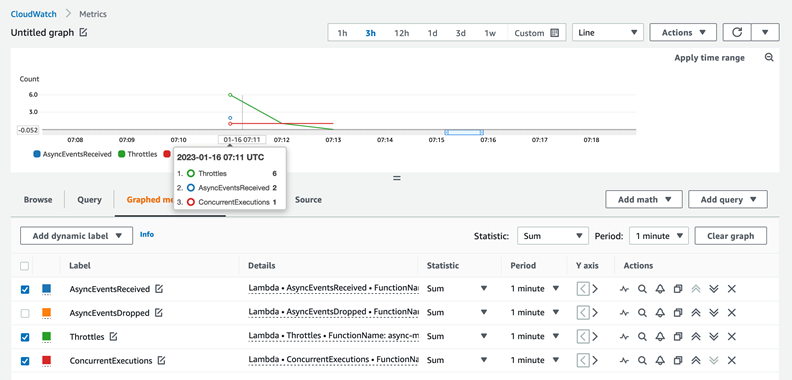
In a real-world use case, missing the processing SLA should trigger the troubleshooting workflow. Start with AsyncEventsReceived to confirm events enqueued by the Lambda service. This is 2 in this scenario. Look for dropped events using AsyncEventsDropped metric.

AsyncEventAge verifies delays in processing. As mentioned in the previous section, there can be multiple data points for this metric in a one-minute interval. You can duplicate the metric to compare minimum and maximum values.

There are 2 data points in the first minute. The event age increases to 31 seconds during this period.

There is only one data point for the metric in the remaining one-minute intervals, so the lines overlap. The event age increases to 59,153ms (~59 seconds) in one interval and then to 130,315ms (~130 seconds) in the next one-minute interval. Since the function sleeps for 90 seconds, it explains why the final retry is at around 2 minutes since the function received the event.
Checking function throttling, this screenshot confirms throttling six times in the first minute (07:12 UTC timestamp) and once in the subsequent minute (07:13 UTC timestamp).

This is because of the back-off behavior of Lambda’s internal queue. The data for AsyncEventAge shows that there is only one throttle in the second interval. Lambda delivers the event during the next one-minute interval after spending around 2 minutes in the internal queue.
Overlaying the ConcurrentExecutions and AsyncEventsReceived metrics provides more information. You see receipt of two events, but concurrency stayed at 1. This results in one event being throttled:
There are multiple ways to resolve throttling errors. You optimize the function to run faster or increase the function or account concurrency limits to address throttling errors.
The sample application covers other scenarios such as troubleshooting dropped events on event expiration, and troubleshooting dropped events when a function’s reserved concurrency is set to zero.
Cleaning up
Use the following command and follow the prompts to clean up the resources:
sam delete lambda-async-metric --region $REGIONConclusion
Using these new CloudWatch metrics, you can gain visibility into the processing of Lambda asynchronous invocations. This blog explained the new metrics AsyncEventsReceived, AsyncEventAge, and AsyncEventsDropped and how to use them to troubleshoot issues. With these new metrics, you can track the asynchronous invocation requests sent to Lambda functions. You monitor any delays in processing, and take corrective actions if required.
The Lambda service sends these new metrics to CloudWatch at no cost to you. However, charges apply for CloudWatch Metric Streams and CloudWatch Alarms. See CloudWatch pricing for more information.
For more serverless learning resources, visit Serverless Land.


 Ramesh Ranganathan is a Senior Partner Solution Architect at AWS. He works with AWS customers and partners to provide guidance on enterprise cloud adoption, application modernization and cloud native development. He is passionate about technology and enjoys experimenting with AWS Serverless services.
 Kamen Sharlandjiev is an Analytics Specialist Solutions Architect and Amazon AppFlow expert. He’s on a mission to make life easier for customers who are facing complex data integration challenges. His secret weapon? Fully managed, low-code AWS services that can get the job done with minimal effort and no coding.
 Amit Shah is a cloud based modern data architecture expert and currently leading AWS Data Analytics practice in Atos. Based in Pune in India, he has 20+ years of experience in data strategy, architecture, design and development. He is on a mission to help organization become data-driven.