Sliding window rate limits in distributed systems

Post Syndicated from Grab Tech original https://engineering.grab.com/frequency-capping

Like many other companies, Grab uses marketing communications to notify users of promotions or other news. If a user receives these notifications from multiple companies, it would be a form of information overload and they might even start considering these communications as spam. Over time, this could lead to some users revoking their consent to receive marketing communications altogether. Hence, it is important to find a rate-limited solution that sends the right amount of communications to our users.

Background

In Grab, marketing emails and push notifications are part of carefully designed campaigns to ensure that users get the right notifications (i.e. based on past orders or usage patterns). Trident is Grab’s in-house tool to compose these campaigns so that they run efficiently at scale. An example of a campaign is scheduling a marketing email blast to 10 million users at 4 pm. Read more about Trident’s architecture here.

Trident relies on Hedwig, another in-house service, to deliver the messages to users. Hedwig does the heavy lifting of delivering large amounts of emails and push notifications to users while maintaining a high query per second (QPS) rate and minimal delay. The following high-level architectural illustration demonstrates the interaction between Trident and Hedwig.
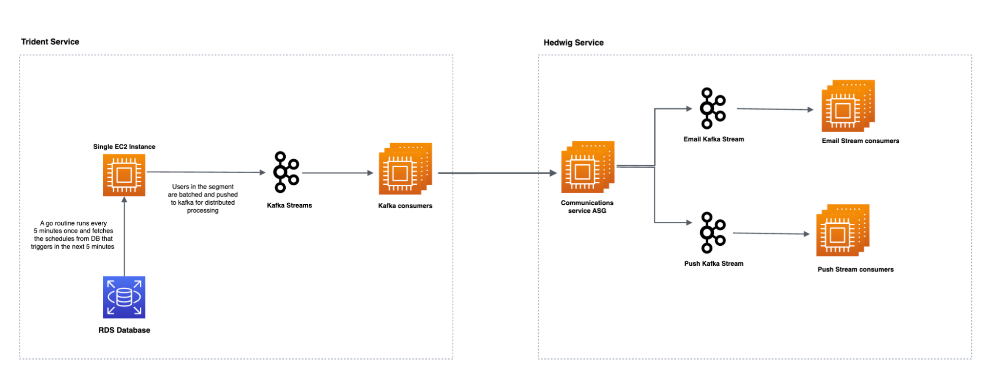
Diagram of data interaction between Trident and Hedwig

The aim is to regulate the number of marketing comms sent to users daily and weekly, tailored based on their interaction patterns with the Grab superapp.

Solution

Based on their interaction patterns with our superapp, we have clustered users into a few segments.

For example:

New: Users recently signed up to the Grab app but haven’t taken any rides yet.
Active: Users who took rides in the past month.

With these metrics, we came up with optimal daily and weekly frequency limit values for each clustered user segment. The solution discussed in this article ensures that the comms sent to a user do not exceed the daily and weekly thresholds for the segment. This is also called frequency capping.

However, frequency capping can be split into two sub-problems:

Efficient storage of clustered user data

With a huge customer base of over 270 million users, storing the user segment membership information has to be cost-efficient and memory-sleek. Querying the segment to which a user belongs should also have minimal latency.

Persistent tracking of comms sent per user

To stay within the daily and weekly thresholds, we need to actively track the number of comms sent to each user, which can be referred to make rate limiting decisions. The rate limiting logic should also have minimal latency, be cost efficient, and not take up too much memory storage.

Optimising storage of user segment data

The problem here is figuring out which segment a particular user belongs to and ensuring that the user doesn’t appear in more than one segment. There are two options that suit our needs and we’ll explain more about each option, as well as what was the best option for us.

Bloom filter 

A Bloom filter is a space-efficient probabilistic data structure that addresses this problem well. Simply put, Bloom filters internally use arrays to track memberships of the elements.

For our scenario, each user segment would need its own bloom filter. We used this bloom filter calculator to estimate the memory required for each bloom filter. We found that we needed approximately 1 GB of memory and 23 hash functions to accurately represent the membership information of 270 million users in an array. Additionally, this method guarantees a false positive rate of  1.0E-7, which means 1 in 1 million elements may get wrong membership results because of hash collision.

With Grab’s existing segments, this approach needs 4GB of memory, which may increase as we increase the number of segments in the future. Moreover, the potential hash collision needs to be handled by increasing the memory size with even more hash functions. Another thing to note is that Bloom filters do not support deletion so every time a change needs to be done, you need to create a new version of the Bloom filter. Although Bloom filters have many advantages, these shortcomings led us to explore another approach.

Roaring bitmaps Roaring bitmaps are sets of unsigned integers consisting of containers of disjoint subsets, which can store large amounts of data in a compressed form. Essentially, roaring bitmaps could reduce memory storage significantly and overcome the hash collision problem. To understand the intuition behind this, first, we need to know how bitmaps work and the possible drawbacks behind it.

To represent a list of numbers as a bitmap, we first need to create an array with a size equivalent to the largest element in the list. For every element in the list, we then mark the bit value as 1 in the corresponding index in the array. While bitmaps work very well for storing integers in closer intervals, they occupy more space and become sparse when storing integer ranges with uneven distribution, as shown in the image below.
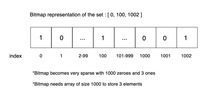
Diagram of bitmaps with uneven distribution

To reduce memory footprint and improve the performance of bitmaps, there are compression techniques such as Run-Length Encoding (RLE), and Word Aligned Hybrid (WAH). However, this would require additional effort to implement, whereas using roaring bitmaps would solve these issues.

Roaring bitmaps’ hybrid data storage approach offers the following advantages:

  • Faster set operations (union, intersection, differencing).
  • Better compression ratio when handling mixed datasets (both dense and sparse data distribution).
  • Ability to scale to large datasets without significant performance loss.

To summarise, roaring bitmaps can store positive integers from 0 to (2^32)-1. Each positive integer value is converted to a 32-bit binary, where the 16 Most Significant Bits (MSB) are used as the key and the remaining 16 Least Significant Bits (LSB) are represented as the value. The values are then stored in an array, a bitmap, or used to run containers with RLE encoding data structures.

If the number of integers mapped to the key is less than 4096, then all the integers are stored in an array in sorted order and converted into a bitmap container in the runtime as the size exceeds. Roaring bitmap analyses the distribution of set bits in the bitmap container i.e. if the continuous interval of set bits is more than a given threshold, the bitmap container can be more efficiently represented using the RLE container. Internally, the RLE container uses an array where the even indices store the beginning of the runs and the odd indices represent the length of the runs. This enables the roaring bitmap to dynamically switch between the containers to optimise storage and performance.

The following diagram shows how a set of elements with different distributions are stored in roaring bitmaps.
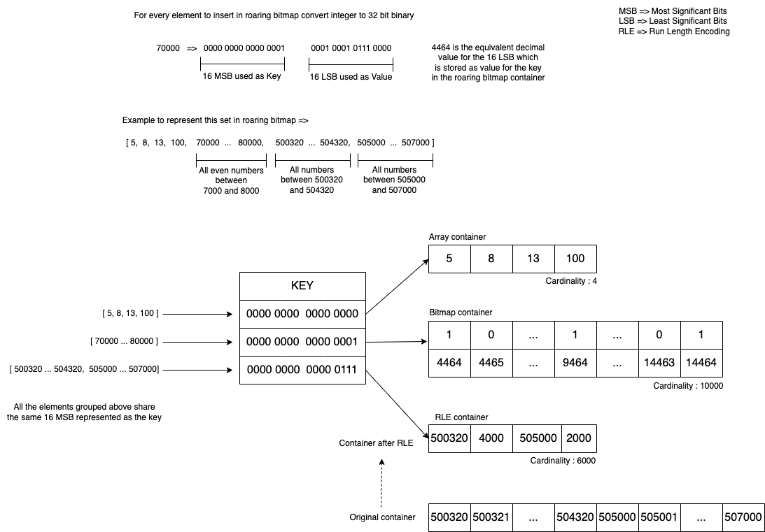
Diagram of how roaring bitmaps store elements with different distributions

In Grab, we developed a microservice that abstracts roaring bitmaps implementations and provides an API to check set membership and enumeration of elements in the sets. Check out this blog to learn more about it.

Distributed rate limiting

The second part of the problem involves rate limiting the number of communication messages sent to users on a daily or weekly basis and each segment has specific daily and weekly limits. By utilising roaring bitmaps, we can determine the segment to which a user belongs. After identifying the appropriate segment, we will apply the personalised limits to the user using a distributed rate limiter, which will be discussed in further detail in the following sections.

Choosing the right datastore

Based on our use case, Amazon ElasticCache for Redis and DynamoDB were two viable options for storing the sent communication messages count per user. However, we decided to choose Redis due to a number of factors:

  • Higher throughput at lower latency – Redis shards data across nodes in the cluster.
  • Cost-effective – Usage of Lua script reduces unnecessary data transfer overheads.
  • Better at handling spiky rate limiting workloads at scale.

Distributed rate limiter

To appropriately limit the comms our users receive, we needed a rate limiting algorithm, which could execute directly in the datastore cluster, then return the results in the application logic for further processing. The two rate limiting algorithms we considered were the sliding window rate limiter and sliding log rate limiter.

The sliding window rate limiter algorithm divides time into a fixed-size window (we defined this as 1 minute) and counts the number of requests within each window. On the other hand, the sliding log maintains a log of each request timestamp and counts the number of requests between two timestamp ranges, providing a more fine-grained method of rate limiting. Although sliding log consumes more memory to store the log of request timestamp, we opted for the sliding log approach as the accuracy of the rate limiting was more important than memory consumption.

The sliding log rate limiter utilises a Redis sorted set data structure to efficiently track and organise request logs. Each timestamp in milliseconds is stored as a unique member in the set. The score assigned to each member represents the corresponding timestamp, allowing for easy sorting in ascending order. This design choice optimises the speed of search operations when querying for the total request count within specific time ranges.

Sliding Log Rate limiter Algorithm:

Input:
  # user specific redis key where the request timestamp logs are stored as sorted set
  keys => user_redis_key

  # limit_value is the limit that needs to be applied for the user
  # start_time_in_millis is the starting point of the time window
  # end_time_in_millis is the ending point of the time window
  # current_time_in_millis is the current time the request is sent
  # eviction_time_in_millis, members in the set whose value is less than this will be evicted from the set

  args => limit_value, start_time_in_millis, end_time_in_millis, current_time_in_millis, eviction_time_in_millis

Output:
  # 0 means not_allowed and 1 means allowed
  response => 0 / 1

Logic:
  # zcount fetches the count of the request timestamp logs falling between the start and the end timestamp
  request_count = zcount user_redis_key start_time_in_millis end_time_in_millis

  response = 0
  # if the count of request logs is less than allowed limits then record the usage by adding current timestamp in sorted set

  if request_count < limit_value then
    zadd user_redis_key current_time_in_millis current_time_in_millis
    response = 1

  # zremrangebyscore removes the members in the sorted set whose score is less than eviction_time_in_millis

  zremrangebyscore user_redis_key -inf eviction_time_in_millis
  return response

This algorithm takes O(log n) time complexity, where n is the number of request logs stored in the sorted set. It is not possible to evict entries in the sorted set like how we have time-to-live (TTL) for Redis keys. To prevent the size of the sorted set from increasing over time, we have a fixed variable eviction_time_in_millis that is passed to the script. The zremrangebyscore command then deletes members from the sorted set whose score is less than eviction_time_in_millis in O(log n) time complexity.

Lua script optimisations

In Redis Cluster mode, all Redis keys accessed by a Lua script must be present on the same node, and they should be passed as part of the KEYS input array of the script. If the script attempts to access keys located on different nodes within the cluster, a CROSSSLOT error will be thrown. Redis keys, or userIDs, are distributed across multiple nodes in the cluster so it is not feasible to send a batch of userIDs within the same Lua script for rate limiting, as this might result in a CROSSSLOT error.

Invoking a separate Lua script call for each user is a possible approach, but it incurs a significant number of network calls, which can be optimised further with the following approach:

  1. Upload the Lua script into the Redis server during the server startup with the SCRIPT LOAD command and we get the SHA1 hash of the script if the upload is successful.
  2. The SHA1 hash can then be used to invoke the Lua script with the EVALSHA command passing the keys and arguments as script input.
  3. Redis pipelining takes in multiple EVALSHA commands that call the Lua script and each invocation corresponds to a userID for getting the rate limiting result.
  4. Redis pipelining groups the EVALSHA Redis commands with Redis keys located on the same nodes internally. It then sends the grouped commands in a single network call to the relevant nodes within the Redis cluster and provides the rate limiting outcome to the client.

Since Redis operates on a single thread, any long-running Lua script can cause other Redis commands to be blocked until the script completes execution. Thus, it’s optimal for the Lua script to execute in under 5 milliseconds. Additionally, the current time is passed as an argument to the script to account for potential variations in time when the script is executed on a node’s replica, which could be caused by clock drift.

By bringing together roaring bitmaps and the distributed rate limiter, this is what our final solution looks like:
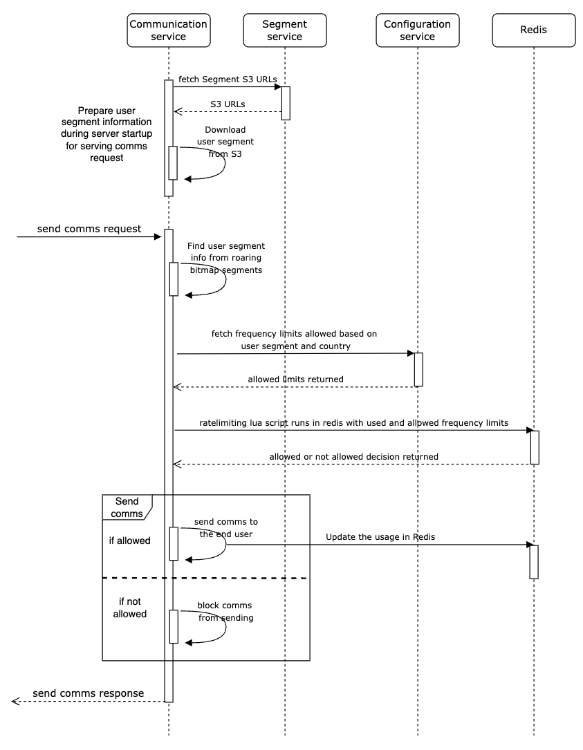
Our final solution using roaring bitmaps and distributed rate limiter

The roaring bitmaps structure is serialised and stored in an AWS S3 bucket, which is then downloaded in the instance during server startup. After which, triggering a user segment membership check can simply be done with a local method call. The configuration service manages the mapping information between the segment and allowed rate limiting values.

Whenever a marketing message needs to be sent to a user, we first find the segment to which the user belongs, retrieve the defined rate limiting values from the configuration service, then execute the Lua script to get the rate limiting decision. If there is enough quota available for the user, we send the comms.

The architecture of the messaging service looks something like this:
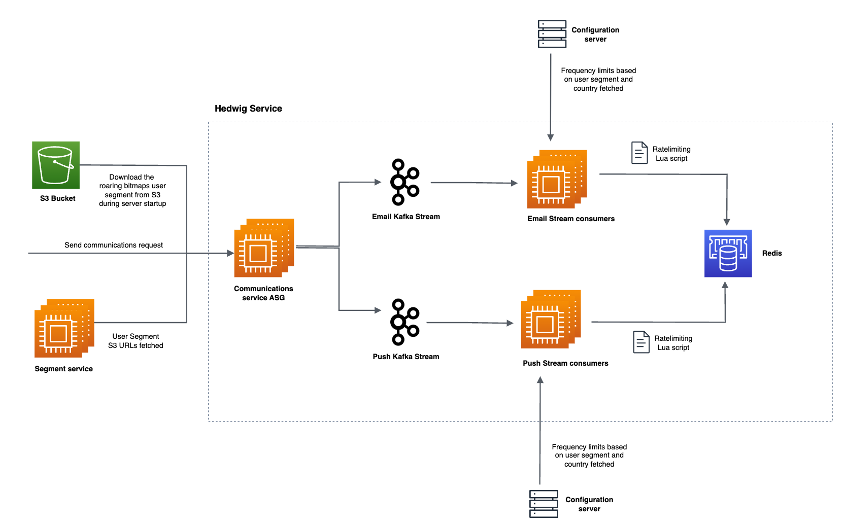
Architecture of the messaging service

Impact

In addition to decreasing the unsubscription rate, there was a significant enhancement in the latency of sending communications. Eliminating redundant communications also alleviated the system load, resulting in a reduction of the delay between the scheduled time and the actual send time of comms.

Conclusion

Applying rate limiters to safeguard our services is not only a standard practice but also a necessary process. Many times, this can be achieved by configuring the rate limiters at the instance level. The need for rate limiters for business logic may not be as common, but when you need it, the solution must be lightning-fast, and capable of seamlessly operating within a distributed environment.

Join us

Grab is the leading superapp platform in Southeast Asia, providing everyday services that matter to consumers. More than just a ride-hailing and food delivery app, Grab offers a wide range of on-demand services in the region, including mobility, food, package and grocery delivery services, mobile payments, and financial services across 428 cities in eight countries.

Powered by technology and driven by heart, our mission is to drive Southeast Asia forward by creating economic empowerment for everyone. If this mission speaks to you, join our team today!

[$] Logo and trademark issues for openSUSE

Post Syndicated from jake original https://lwn.net/Articles/954760/

A contest for new logos
for the openSUSE project and for
four separate distributions of it,
Tumbleweed, Leap, Slowroll, and
Kalpa, has turned into a
bit of an uproar in that community. A vote
has been held on the candidates
and winners have been announced, but
some are questioning why there is a need to change the existing logo (the
“Geeko”
chameleon) at all. In addition, there are questions about whether the
new logo will be trademarked (as previous ones have been)—and how many
years that will take.

GitHub Availability Report: November 2023

Post Syndicated from Jakub Oleksy original https://github.blog/2023-12-13-github-availability-report-november-2023/

In November, we experienced one incident that resulted in degraded performance across GitHub services.

November 3 18:42 UTC (lasting 38 minutes)

Between 18:42 and 19:20 UTC on November 3, the GitHub authorization service experienced excessive application memory use, leading to failed authorization requests and users getting 404 or error responses on most page and API requests.

A performance and resilience optimization to the authorization microservice contained a memory leak that was exposed under high traffic. Testing did not expose the service to sufficient traffic to discover the leak, allowing it to graduate to production at 18:37 UTC. The memory leak under high load caused pods to crash repeatedly starting at 18:42 UTC, failing authorization checks in their default closed state. These failures started triggering alerts at 18:44 UTC. Rolling back the authorization service change was delayed as parts of the deployment infrastructure relied on the authorization service and required manual intervention to complete. Rollback completed at 19:08 UTC and all impacted GitHub features recovered after pods came back online.

To reduce the risk of future deployments, we implemented changes to our rollout strategy by including additional monitoring and checks, which automatically block a deployment from proceeding if key metrics are not satisfactory. To reduce our time to recover in the future, we have removed dependencies between the authorization service and the tools needed to roll back changes.


Please follow our status page for real-time updates on status changes and post-incident recaps. To learn more about what we’re working on, check out the GitHub Engineering Blog.

The post GitHub Availability Report: November 2023 appeared first on The GitHub Blog.

Rust for Linux — in space

Post Syndicated from corbet original https://lwn.net/Articles/954974/

The Rust for Linux (RFL) project may not have (yet) resulted in user-visible
changes to the Linux kernel, but it seems the wider world has taken notice.
Hongyu Li has announced
that the Rust for Linux code is now part of a satellite just launched
out of China. The satellite is running a system called RROS, which follows the old
RTLinux pattern of running a realtime kernel alongside Linux. The realtime
core is written in Rust, using the RFL groundwork.

Despite its imperfections, we still want to share RROS with the
community, showcasing our serious commitment to using RFL for
substantial projects and contributing to the community’s
growth. Our development journey with RROS has been greatly enriched
by the support and knowledge from the RFL community. We also have
received invaluable assistance from enthusiastic forks here,
especially when addressing issues related to safety abstraction

(Thanks to Dirk Behme).

Governance at scale: Enforce permissions and compliance by using policy as code

Post Syndicated from Roland Odorfer original https://aws.amazon.com/blogs/security/governance-at-scale-enforce-permissions-and-compliance-by-using-policy-as-code/

AWS Identity and Access Management (IAM) policies are at the core of access control on AWS. They enable the bundling of permissions, helping to provide effective and modular access control for AWS services. Service control policies (SCPs) complement IAM policies by helping organizations enforce permission guardrails at scale across their AWS accounts.

The use of access control policies isn’t limited to AWS resources. Customer applications running on AWS infrastructure can also use policies to help control user access. This often involves implementing custom authorization logic in the program code itself, which can complicate audits and policy changes.

To address this, AWS developed Amazon Verified Permissions, which helps implement fine-grained authorizations and permissions management for customer applications. This service uses Cedar, an open-source policy language, to define permissions separately from application code.

In addition to access control, you can also use policies to help monitor your organization’s individual governance rules for security, operations and compliance. One example of such a rule is the regular rotation of cryptographic keys to help reduce the impact in the event of a key leak.

However, manually checking and enforcing such rules is complex and doesn’t scale, particularly in fast-growing IT organizations. Therefore, organizations should aim for an automated implementation of such rules. In this blog post, I will show you how to use policy as code to help you govern your AWS landscape.

Policy as code

Similar to infrastructure as code (IaC), policy as code is an approach in which you treat policies like regular program code. You define policies in the form of structured text files (policy documents), which policy engines can automatically evaluate.

The main advantage of this approach is the ability to automate key governance tasks, such as policy deployment, enforcement, and auditing. By storing policy documents in a central repository, you can use versioning, simplify audits, and track policy changes. Furthermore, you can subject new policies to automated testing through integration into a continuous integration and continuous delivery (CI/CD) pipeline. Policy as code thus forms one of the key pillars of a modern automated IT governance strategy.

The following sections describe how you can combine different AWS services and functions to integrate policy as code into existing IT governance processes.

Access control – AWS resources

Every request to AWS control plane resources (specifically, AWS APIs)—whether through the AWS Management Console, AWS Command Line Interface (AWS CLI), or SDK — is authenticated and authorized by IAM. To determine whether to approve or deny a specific request, IAM evaluates both the applicable policies associated with the requesting principal (human user or workload) and the respective request context. These policies come in the form of JSON documents and follow a specific schema that allows for automated evaluation.

IAM supports a range of different policy types that you can use to help protect your AWS resources and implement a least privilege approach. For an overview of the individual policy types and their purpose, see Policies and permissions in IAM. For some practical guidance on how and when to use them, see IAM policy types: How and when to use them. To learn more about the IAM policy evaluation process and the order in which IAM reviews individual policy types, see Policy evaluation logic.

Traditionally, IAM relied on role-based access control (RBAC) for authorization. With RBAC, principals are assigned predefined roles that grant only the minimum permissions needed to perform their duties (also known as a least privilege approach). RBAC can seem intuitive initially, but it can become cumbersome at scale. Every new resource that you add to AWS requires the IAM administrator to manually update each role’s permissions – a tedious process that can hamper agility in dynamic environments.

In contrast, attribute-based access control (ABAC) bases permissions on the attributes assigned to users and resources. IAM administrators define a policy that allows access when certain tags match. ABAC is especially advantageous for dynamic, fast-growing organizations that have outgrown the RBAC model. To learn more about how to implement ABAC in an AWS environment, see Define permissions to access AWS resources based on tags.

For a list of AWS services that IAM supports and whether each service supports ABAC, see AWS services that work with IAM.

Access control – Customer applications

Customer applications that run on AWS resources often require an authorization mechanism that can control access to the application itself and its individual functions in a fine-grained manner.

Many customer applications come with custom authorization mechanisms in the application code itself, making it challenging to implement policy changes. This approach can also hinder monitoring and auditing because the implementation of authorization logic often differs between applications, and there is no uniform standard.

To address this challenge, AWS developed Amazon Verified Permissions and the associated open-source policy language Cedar. Amazon Verified Permissions replaces the custom authorization logic in the application code with a simple IsAuthorized API call, so that you can control and monitor authorization logic centrally by using Cedar-based policies. To learn how to integrate Amazon Verified Permissions into your applications and define custom access control policies with Cedar, see How to use Amazon Verified Permissions for authorization.

Compliance

In addition to access control, you can also use policies to help monitor and enforce your organization’s individual governance rules for security, operations and compliance. AWS Config and AWS Security Hub play a central role in compliance because they enable the setup of multi-account environments that follow best practices (known as landing zones). AWS Config continuously tracks resource configurations and changes, while Security Hub aggregates and prioritizes security findings. With these services, you can create controls that enable automated audits and conformity checks. Alternatively, you can also choose from ready-to-use controls that cover individual compliance objectives such as encryption at rest, or entire frameworks, such as PCI-DSS and NIST 800-53.

AWS Control Tower builds on top of AWS Config and Security Hub to help simplify governance and compliance for multi-account environments. AWS Control Tower incorporates additional controls with the existing ones from AWS Config and Security Hub, presenting them together through a unified interface. These controls apply at different resource life cycle stages, as shown in Figure 1, and you define them through policies.

Figure 1: Resource life cycle

Figure 1: Resource life cycle

The controls can be categorized according to their behavior:

  • Proactive controls scan IaC templates before deployment to help identify noncompliance issues early.
  • Preventative controls restrict actions within an AWS environment to help prevent noncompliant actions. For example, these controls can help prevent deployment of large Amazon Elastic Compute Cloud (Amazon EC2) instances or restrict the available AWS Regions for some users.
  • Detective controls monitor deployed resources to help identify noncompliant resources that proactive and preventative controls might have missed. They also detect when deployed resources are changed or drift out of compliance over time.

Categorizing controls this way allows for a more comprehensive compliance framework that encompasses the entire resource life cycle. The stage at which each control applies determines how it may help enforce policies and governance rules.

With AWS Control Tower, you can enable hundreds of preconfigured security, compliance, and operational controls through the console with a single click, without needing to write code. You can also implement your own custom controls beyond what AWS Control Tower provides out of the box. The process for implementing custom controls varies depending on the type of control. In the following sections, I will explain how to set up custom controls for each type.

Proactive controls

Proactive controls are mechanisms that scan resources and their configuration to confirm that they adhere to compliance requirements before they are deployed. AWS provides a range of tools and services that you can use, both in isolation and in combination with each other, to implement proactive controls. The following diagram provides an overview of the available mechanisms and an example of their integration into a CI/CD pipeline for AWS Cloud Development Kit (CDK) projects.

Figure 2: CI/CD pipeline in AWS CDK projects

Figure 2: CI/CD pipeline in AWS CDK projects

As shown in Figure 2, you can use the following mechanisms as proactive controls:

  1. You can validate artifacts such as IaC templates locally on your machine by using the AWS CloudFormation Guard CLI, which facilitates a shift-left testing strategy. The advantage of this approach is the relatively early testing in the deployment cycle. This supports rapid iterative development and thus reduces waiting times.

    Alternatively, you can use the CfnGuardValidator plugin for AWS CDK, which integrates CloudFormation Guard rules into the AWS CDK CLI. This streamlines local development by applying policies and best practices directly within the CDK project.

  2. To centrally enforce validation checks, integrate the CfnGuardValidator plugin into a CDK CI/CD pipeline.
  3. You can also invoke the CloudFormation Guard CLI from within AWS CodeBuild buildspecs to embed CloudFormation Guard scans in a CI/CD pipeline.
  4. With CloudFormation hooks, you can impose policies on resources before CloudFormation deploys them.

AWS CloudFormation Guard uses a policy-as-code approach to evaluate IaC documents such as AWS CloudFormation templates and Terraform configuration files. The tool defines validation rules in the Guard language to check that these JSON or YAML documents align with best practices and organizational policies around provisioning cloud resources. By codifying rules and scanning infrastructure definitions programmatically, CloudFormation Guard automates policy enforcement and helps promote consistency and security across infrastructure deployments.

In the following example, you will use CloudFormation Guard to validate the name of an Amazon Simple Storage Service (Amazon S3) bucket in a CloudFormation template through a simple Guard rule:

To validate the S3 bucket

  1. Install CloudFormation Guard locally. For instructions, see Setting up AWS CloudFormation Guard.
  2. Create a YAML file named template.yaml with the following content and replace <DOC-EXAMPLE-BUCKET> with a bucket name of your choice (this file is a CloudFormation template, which creates an S3 bucket):
    Resources:
      S3Bucket:
        Type: 'AWS::S3::Bucket'
        Properties:
          BucketName: '<DOC-EXAMPLE-BUCKET>'

  3. Create a text file named rules.guard with the following content:
    rule checkBucketName {
        Resources.S3Bucket.Properties.BucketName == '<DOC-EXAMPLE-BUCKET>'
    }

  4. To validate your CloudFormation template against your Guard rules, run the following command in your local terminal:
    cfn-guard validate --rules rules.guard --data template.yaml

  5. If CloudFormation Guard successfully validates the template, the validate command produces an exit status of 0 ($? in bash). Otherwise, it returns a status report listing the rules that failed. You can test this yourself by changing the bucket name.

To accelerate the writing of Guard rules, use the CloudFormation Guard rulegen command, which takes a CloudFormation template file as an input and autogenerates Guard rules that match the properties of the template resources. To learn more about the structure of CloudFormation Guard rules and how to write them, see Writing AWS CloudFormation Guard rules.

The AWS Guard Rules Registry provides ready-to-use CloudFormation Guard rule files to accelerate your compliance journey, so that you don’t have to write them yourself.

Through the CDK plugin interface for policy validation, the CfnGuardValidator plugin integrates CloudFormation Guard rules into the AWS CDK and validates generated CloudFormation templates automatically during its synthesis step. For more details, see the plugin documentation and Accelerating development with AWS CDK plugin – CfnGuardValidator.

CloudFormation Guard alone can’t necessarily prevent the provisioning of noncompliant resources. This is because CloudFormation Guard can’t detect when templates or other documents change after validation. Therefore, I recommend that you combine CloudFormation Guard with a more authoritative mechanism.

One such mechanism is CloudFormation hooks, which you can use to validate AWS resources before you deploy them. You can configure hooks to cancel the deployment process with an alert if CloudFormation templates aren’t compliant, or just initiate an alert but complete the process. To learn more about CloudFormation hooks, see the following blog posts:

CloudFormation hooks provide a way to authoritatively enforce rules for resources deployed through CloudFormation. However, they don’t control resource creation that occurs outside of CloudFormation, such as through the console, CLI, SDK, or API. Terraform is one example that provisions resources directly through the AWS API rather than through CloudFormation templates. Because of this, I recommend that you implement additional detective controls by using AWS Config. AWS Config can continuously check resource configurations after deployment, regardless of the provisioning method. Using AWS Config rules complements the preventative capabilities of CloudFormation hooks.

Preventative controls

Preventative controls can help maintain compliance by applying guardrails that disallow policy-violating actions. AWS Control Tower integrates with AWS Organizations to implement preventative controls with SCPs. By using SCPs, you can restrict IAM permissions granted in a given organization or organizational unit (OU). One example of this is the selective activation of certain AWS Regions to meet data residency requirements.

SCPs are particularly valuable for managing IAM permissions across large environments with multiple AWS accounts. Organizations with many accounts might find it challenging to monitor and control IAM permissions. SCPs help address this challenge by applying centralized permission guardrails automatically to the accounts of an organization or organizational unit (OU). As new accounts are added, the SCPs are enforced without the need for extra configuration.

You can define SCPs through CloudFormation or CDK templates and deploy them through a CI/CD pipeline, similar to other AWS resources. Because misconfigured SCPs can negatively affect an organization’s operations, it’s vital that you test and simulate the effects of new policies in a sandbox environment before broader deployment. For an example of how to implement a pipeline for SCP testing, see the aws-service-control-policies-deployment GitHub repository.

To learn more about SCPs and how to implement them, see Service control policies (SCPs) and Best Practices for AWS Organizations Service Control Policies in a Multi-Account Environment.

Detective controls

Detective controls help detect noncompliance with existing resources. You can implement detective controls by using AWS Config rules, with both managed rules (provided by AWS) and custom rules available. You can implement custom rules either by using the domain-specific language Guard or Lambda functions. To learn more about the Guard option, see Evaluate custom configurations using AWS Config Custom Policy rules and the open source sample repository. For guidance on creating custom rules using Lambda functions, see AWS Config Rule Development Kit library: Build and operate rules at scale and Deploying Custom AWS Config Rules in an AWS Organization Environment.

To simplify audits for compliance frameworks such as PCI-DSS, HIPAA, and SOC2, AWS Config also offers conformance packs that bundle rules and remediation actions. To learn more about conformance packs, see Conformance Packs and Introducing AWS Config Conformance Packs.

When a resource’s configuration shifts to a noncompliant state that preventive controls didn’t avert, detective controls can help remedy the noncompliant state by implementing predefined actions, such as alerting an operator or reconfiguring the resource. You can implement these controls with AWS Config, which integrates with AWS Systems Manager Automation to help enable the remediation of noncompliant resources.

Security Hub can help centralize the detection of noncompliant resources across multiple AWS accounts. Using AWS Config and third-party tools for detection, Security Hub sends findings of noncompliance to Amazon EventBridge, which can then send notifications or launch automated remediations. You can also use the security controls and standards in Security Hub to monitor the configuration of your AWS infrastructure. This complements the conformance packs in AWS Config.

Conclusion

Many large and fast-growing organizations are faced with the challenge that manual IT governance processes are difficult to scale and can hinder growth. Policy-as-code services help to manage permissions and resource configurations at scale by automating key IT governance processes and, at the same time, increasing the quality and transparency of those processes. This helps to reconcile large environments with key governance objectives such as compliance.

In this post, you learned how to use policy as code to enhance IT governance. A first step is to activate AWS Control Tower, which provides preconfigured guardrails (SCPs) for each AWS account within an organization. These guardrails help enforce baseline compliance across infrastructure. You can then layer on additional controls to further strengthen governance in line with your needs. As a second step, you can select AWS Config conformance packs and Security Hub standards to complement the controls that AWS Control Tower offers. Finally, you can secure applications built on AWS by using Amazon Verified Permissions and Cedar for fine-grained authorization.

Resources

 
If you have feedback about this post, submit comments in the Comments section below. If you have questions about this post, contact AWS Support.

Want more AWS Security news? Follow us on Twitter.

Roland Odorfer

Roland Odorfer

Roland is a Solutions Architect at AWS, based in Berlin, Germany. He works with German industry and manufacturing customers, helping them architect secure and scalable solutions. Roland is interested in distributed systems and security. He enjoys helping customers use the cloud to solve complex challenges.

How to Run AI/ML Workloads on CoreWeave + Backblaze

Post Syndicated from Pat Patterson original https://www.backblaze.com/blog/how-to-run-ai-ml-workloads-on-coreweave-backblaze/

A decorative image showing the Backblaze and CoreWeave logos superimposed on clouds.

Backblaze compute partner CoreWeave is a specialized GPU cloud provider designed to power use cases such as AI/ML, graphics, and rendering up to 35x faster and for 80% less than generalized public clouds. Brandon Jacobs, an infrastructure architect at CoreWeave, joined us earlier this year for Backblaze Tech Day ‘23. Brandon and I co-presented a session explaining both how to backup CoreWeave Cloud storage volumes to Backblaze B2 Cloud Storage and how to load a model from Backblaze B2 into the CoreWeave Cloud inference stack.

Since we recently published an article covering the backup process, in this blog post I’ll focus on loading a large language model (LLM) directly from Backblaze B2 into CoreWeave Cloud.

Below is the session recording from Tech Day; feel free to watch it instead of, or in addition to, reading this article.

More About CoreWeave

In the Tech Day session, Brandon covered the two sides of CoreWeave Cloud: 

  1. Model training and fine tuning. 
  2. The inference service. 

To maximize performance, CoreWeave provides a fully-managed Kubernetes environment running on bare metal, with no hypervisors between your containers and the hardware.

CoreWeave provides a range of storage options: storage volumes that can be directly mounted into Kubernetes pods as block storage or a shared file system, running on solid state drives (SSDs) or hard disk drives (HDDs), as well as their own native S3 compatible object storage. Knowing that, you’re probably wondering, “Why bother with Backblaze B2, when CoreWeave has their own object storage?”

The answer echoes the first few words of this blog post—CoreWeave’s object storage is a specialized implementation, co-located with their GPU compute infrastructure, with high-bandwidth networking and caching. Backblaze B2, in contrast, is general purpose cloud object storage, and includes features such as Object Lock and lifecycle rules, that are not as relevant to CoreWeave’s object storage. There is also a price differential. Currently, at $6/TB/month, Backblaze B2 is one-fifth of the cost of CoreWeave’s object storage.

So, as Brandon and I explained in the session, CoreWeave’s native storage is a great choice for both the training and inference use cases, where you need the fastest possible access to data, while Backblaze B2 shines as longer term storage for training, model, and inference data as well as the destination for data output from the inference process. In addition, since Backblaze and CoreWeave are bandwidth partners, you can transfer data between our two clouds with no egress fees, freeing you from unpredictable data transfer costs.

Loading an LLM From Backblaze B2

To demonstrate how to load an archived model from Backblaze B2, I used CoreWeave’s GPT-2 sample. GPT-2 is an earlier version of the GPT-3.5 and GPT-4 LLMs used in ChatGPT. As such, it’s an accessible way to get started with LLMs, but, as you’ll see, it certainly doesn’t pass the Turing test!

This sample comprises two applications: a transformer and a predictor. The transformer implements a REST API, handling incoming prompt requests from client apps, encoding each prompt into a tensor, which the transformer passes to the predictor. The predictor applies the GPT-2 model to the input tensor, returning an output tensor to the transformer for decoding into text that is returned to the client app. The two applications have different hardware requirements—the predictor needs a GPU, while the transformer is satisfied with just a CPU, so they are configured as separate Kubernetes pods, and can be scaled up and down independently.

Since the GPT-2 sample includes instructions for loading data from Amazon S3, and Backblaze B2 features an S3 compatible API, it was a snap to modify the sample to load data from a Backblaze B2 Bucket. In fact, there was just a single line to change, in the s3-secret.yaml configuration file. The file is only 10 lines long, so here it is in its entirety:

apiVersion: v1
kind: Secret
metadata:
  name: s3-secret
  annotations:
     serving.kubeflow.org/s3-endpoint: s3.us-west-004.backblazeb2.com
type: Opaque
data:
  AWS_ACCESS_KEY_ID: <my-backblaze-b2-application-key-id>
  AWS_SECRET_ACCESS_KEY: <my-backblaze-b2-application-key>

As you can see, all I had to do was set the serving.kubeflow.org/s3-endpoint metadata annotation to my Backblaze B2 Bucket’s endpoint and paste in an application key and its ID.

While that was the only Backblaze B2-specific edit, I did have to configure the bucket and path where my model was stored. Here’s an excerpt from gpt-s3-inferenceservice.yaml, which configures the inference service itself:

apiVersion: serving.kubeflow.org/v1alpha2
kind: InferenceService
metadata:
  name: gpt-s3
  annotations:
    # Target concurrency of 4 active requests to each container
    autoscaling.knative.dev/target: "4"
    serving.kubeflow.org/gke-accelerator: Tesla_V100
spec:
  default:
    predictor:
      minReplicas: 0 # Allow scale to zero
      maxReplicas: 2 
      serviceAccountName: s3-sa # The B2 credentials are retrieved from the service account
      tensorflow:
        # B2 bucket and path where the model is stored
        storageUri: s3://<my-bucket>/model-storage/124M/
        runtimeVersion: "1.14.0-gpu"
        ...

Aside from storageUri configuration, you can see how the predictor application’s pod is configured to scale from between zero and two instances (“replicas” in Kubernetes terminology). The remainder of the file contains the transformer pod configuration, allowing it to scale from zero to a single instance.

Running an LLM on CoreWeave Cloud

Spinning up the inference service involved a kubectl apply command for each configuration file and a short wait for the CoreWeave GPU cloud to bring up the compute and networking infrastructure. Once the predictor and transformer services were ready, I used curl to submit my first prompt to the transformer endpoint:

% curl -d '{"instances": ["That was easy"]}' http://gpt-s3-transformer-default.tenant-dead0a.knative.chi.coreweave.com/v1/models/gpt-s3:predict
{"predictions": ["That was easy for some people, it's just impossible for me,\" Davis said. \"I'm still trying to" ]}

In the video, I repeated the exercise, feeding GPT-2’s response back into it as a prompt a few times to generate a few paragraphs of text. Here’s what it came up with:

“That was easy: If I had a friend who could take care of my dad for the rest of his life, I would’ve known. If I had a friend who could take care of my kid. He would’ve been better for him than if I had to rely on him for everything.

The problem is, no one is perfect. There are always more people to be around than we think. No one cares what anyone in those parts of Britain believes,

The other problem is that every decision the people we’re trying to help aren’t really theirs. If you have to choose what to do”

If you’ve used ChatGPT, you’ll recognize how far LLMs have come since GPT-2’s release in 2019!

Run Your Own Large Language Model

While CoreWeave’s GPT-2 sample is an excellent introduction to the world of LLMs, it’s a bit limited. If you’re looking to get deeper into generative AI, another sample, Fine-tune Large Language Models with CoreWeave Cloud, shows how to fine-tune a model from the more recent EleutherAI Pythia suite.

Since CoreWeave is a specialized GPU cloud designed to deliver best-in-class performance up to 35x faster and 80% less expensive than generalized public clouds, it’s a great choice for workloads such as AI, ML, rendering, and more, and, as you’ve seen in this blog post, easy to integrate with Backblaze B2 Cloud Storage, with no data transfer costs. For more information, contact the CoreWeave team.

The post How to Run AI/ML Workloads on CoreWeave + Backblaze appeared first on Backblaze Blog | Cloud Storage & Cloud Backup.

OpenPGP for application developers

Post Syndicated from corbet original https://lwn.net/Articles/954964/

A new book called OpenPGP for application
developers
has been released under the Creative Commons BY-SA license.

This document is not intended for end-users or implementers of
OpenPGP libraries (or other software that directly handles internal
OpenPGP data structures).

Instead, this document is focused on the second group, application
developers, who use OpenPGP functionality in their software
projects. It describes the properties of the OpenPGP system and its
uses. It presupposes solid knowledge of software development
concepts and of general cryptographic concepts. Thus, this text
describes OpenPGP at the “library-level,” teaching concepts that
will help software developers get started as a user of any
implementation (e.g., OpenPGP.js, Sequoia-PGP).

Modernize your ETL platform with AWS Glue Studio: A case study from BMS

Post Syndicated from Sivaprasad Mahamkali original https://aws.amazon.com/blogs/big-data/modernize-your-etl-platform-with-aws-glue-studio-a-case-study-from-bms/

This post is co-written with Ramesh Daddala, Jitendra Kumar Dash and Pavan Kumar Bijja from Bristol Myers Squibb.

Bristol Myers Squibb (BMS) is a global biopharmaceutical company whose mission is to discover, develop, and deliver innovative medicines that help patients prevail over serious diseases. BMS is consistently innovating, achieving significant clinical and regulatory successes. In collaboration with AWS, BMS identified a business need to migrate and modernize their custom extract, transform, and load (ETL) platform to a native AWS solution to reduce complexities, resources, and investment to upgrade when new Spark, Python, or AWS Glue versions are released. In addition to using native managed AWS services that BMS didn’t need to worry about upgrading, BMS was looking to offer an ETL service to non-technical business users that could visually compose data transformation workflows and seamlessly run them on the AWS Glue Apache Spark-based serverless data integration engine. AWS Glue Studio is a graphical interface that makes it easy to create, run, and monitor ETL jobs in AWS Glue. Offering this service reduced BMS’s operational maintenance and cost, and offered flexibility to business users to perform ETL jobs with ease.

For the past 5 years, BMS has used a custom framework called Enterprise Data Lake Services (EDLS) to create ETL jobs for business users. Although this framework met their ETL objectives, it was difficult to maintain and upgrade. BMS’s EDLS platform hosts over 5,000 jobs and is growing at 15% YoY (year over year). Each time the newer version of Apache Spark (and corresponding AWS Glue version) was released, it required significant operational support and time-consuming manual changes to upgrade existing ETL jobs. Manually upgrading, testing, and deploying over 5,000 jobs every few quarters was time consuming, error prone, costly, and not sustainable. Because another release for the EDLS framework was pending, BMS decided to assess alternate managed solutions to reduce their operational and upgrade challenges.

In this post, we share how BMS will modernize leveraging the success of the proof of concept targeting BMS’s ETL platform using AWS Glue Studio.

Solution overview

This solution addresses BMS’s EDLS requirements to overcome challenges using a custom-built ETL framework that required frequent maintenance and component upgrades (requiring extensive testing cycles), avoid complexity, and reduce the overall cost of the underlying infrastructure derived from the proof of concept. BMS had the following goals:

  • Develop ETL jobs using visual workflows provided by the AWS Glue Studio visual editor. The AWS Glue Studio visual editor is a low-code environment that allows you to compose data transformation workflows, seamlessly run them on the AWS Glue Apache Spark-based serverless data integration engine, and inspect the schema and data results in each step of the job.
  • Migrate over 5,000 existing ETL jobs using native AWS Glue Studio in an automated and scalable manner.

EDLS job steps and metadata

Every EDLS job comprises one or more job steps chained together and run in a predefined order orchestrated by the custom ETL framework. Each job step incorporates the following ETL functions:

  • File ingest – File ingestion enables you to ingest or list files from multiple file sources, like Amazon Simple Storage Service (Amazon S3), SFTP, and more. The metadata holds configurations for the file ingestion step to connect to Amazon S3 or SFTP endpoints and ingest files to target location. It retrieves the specified files and available metadata to show on the UI.
  • Data quality check – The data quality module enables you to perform quality checks on a huge amount of data and generate reports that describe and validate the data quality. The data quality step uses an EDLS ingested source object from Amazon S3 and runs one to many data conformance checks that are configured by the tenant.
  • Data transform join – This is one of the submodules of the data transform module that can perform joins between the datasets using a custom SQL based on the metadata configuration.
  • Database ingest – The database ingestion step is one of the important service components in EDLS, which facilitates you to obtain and import the desired data from the database and export it to a specific file in the location of your choice.
  • Data transform – The data transform module performs various data transformations against the source data using JSON-driven rules. Each data transform capability has its own JSON rule and, based on the specific JSON rule you provide, EDLS performs the data transformation on the files available in the Amazon S3 location.
  • Data persistence – The data persistence module is one of the important service components in EDLS, which enables you to obtain the desired data from the source and persist it to an Amazon Relational Database Service (Amazon RDS) database.

The metadata corresponding to each job step includes ingest sources, transformation rules, data quality checks, and data destinations stored in an RDS instance.

Migration utility

The solution involves building a Python utility that reads EDLS metadata from the RDS database and translating each of the job steps into an equivalent AWS Glue Studio visual editor JSON node representation.

AWS Glue Studio provides two types of transforms:

  • AWS Glue-native transforms – These are available to all users and are managed by AWS Glue.
  • Custom visual transforms – This new functionality allows you to upload custom-built transforms used in AWS Glue Studio. Custom visual transforms expand the managed transforms, enabling you to search and use transforms from the AWS Glue Studio interface.

The following is a high-level diagram depicting the sequence flow of migrating a BMS EDLS job to an AWS Glue Studio visual editor job.

Migrating BMS EDLS jobs to AWS Glue Studio includes the following steps:

  1. The Python utility reads existing metadata from the EDLS metadata database.
  2. For each job step type, based on the job metadata, the Python utility selects either the native AWS Glue transform, if available, or a custom-built visual transform (when the native functionality is missing).
  3. The Python utility parses the dependency information from metadata and builds a JSON object representing a visual workflow represented as a Directed Acyclic Graph (DAG).
  4. The JSON object is sent to the AWS Glue API, creating the AWS Glue ETL job. These jobs are visually represented in the AWS Glue Studio visual editor using a series of sources, transforms (native and custom), and targets.

Sample ETL job generation using AWS Glue Studio

The following flow diagram depicts a sample ETL job that incrementally ingests the source RDBMS data in AWS Glue based on modified timestamps using a custom SQL and merges it into the target data on Amazon S3.

The preceding ETL flow can be represented using the AWS Glue Studio visual editor through a combination of native and custom visual transforms.

Custom visual transform for incremental ingestion

Post POC, BMS and AWS identified there will be a need to leverage custom transforms to execute a subset of jobs leveraging their current EDLS Service where Glue Studio functionality will not be a natural fit. The BMS team’s requirement was to ingest data from various databases without depending on the existence of transaction logs or specific schema, so AWS Database Migration Service (AWS DMS) wasn’t an option for them. AWS Glue Studio provides the native SQL query visual transform, where a custom SQL query can be used to transform the source data. However, in order to query the source database table based on a modified timestamp column to retrieve new and modified records since the last ETL run, the previous timestamp column state needs to be persisted so it can be used in the current ETL run. This needs to be a recurring process and can also be abstracted across various RDBMS sources, including Oracle, MySQL, Microsoft SQL Server, SAP Hana, and more.

AWS Glue provides a job bookmark feature to track the data that has already been processed during a previous ETL run. An AWS Glue job bookmark supports one or more columns as the bookmark keys to determine new and processed data, and it requires that the keys are sequentially increasing or decreasing without gaps. Although this works for many incremental load use cases, the requirement is to ingest data from different sources without depending on any specific schema, so we didn’t use an AWS Glue job bookmark in this use case.

The SQL-based incremental ingestion pull can be developed in a generic way using a custom visual transform using a sample incremental ingestion job from a MySQL database. The incremental data is merged into the target Amazon S3 location in Apache Hudi format using an upsert write operation.

In the following example, we’re using the MySQL data source node to define the connection but the DynamicFrame of the data source itself is not used. The custom transform node (DB incremental ingestion) will act as the source for reading the data incrementally using the custom SQL query and the previously persisted timestamp from the last ingestion.

The transform accepts as input parameters the preconfigured AWS Glue connection name, database type, table name, and custom SQL (parameterized timestamp field).

The following is the sample visual transform Python code:

import boto3
from awsglue import DynamicFrame
from datetime import datetime

region_name = "us-east-1"

dyna_client = boto3.client('dynamodb')
HISTORIC_DATE = datetime(1970,1,1).strftime("%Y-%m-%d %H:%M:%S")
DYNAMODB_TABLE = "edls_run_stats"

def db_incremental(self, transformation_node, con_name, con_type, table_name, sql_query):
    logger = self.glue_ctx.get_logger()

    last_updt_tmst = get_table_last_updt_tmst(logger, DYNAMODB_TABLE, transformation_node)

    logger.info(f"Last updated timestamp from the DynamoDB-> {last_updt_tmst}")

    sql_query = sql_query.format(**{"lastmdfdtmst": last_updt_tmst})

    connection_options_source = {
        "useConnectionProperties": "true",
        "connectionName": con_name,
        "dbtable": table_name,
        "sampleQuery": sql_query
    }

    df = self.glue_ctx.create_dynamic_frame.from_options(connection_type= con_type, connection_options= connection_options_source )
                                         
    return df

DynamicFrame.db_incremental = db_incremental

def get_table_last_updt_tmst(logger, table_name, transformation_node):
    response = dyna_client.get_item(TableName=table_name,
                                    Key={'transformation_node': {'S': transformation_node}}
                                    )
    if 'Item' in response and 'last_updt_tmst' in response['Item']:
        return response['Item']['last_updt_tmst']['S']
    else:
        return HISTORIC_DATE

To merge the source data into the Amazon S3 target, a data lake framework like Apache Hudi or Apache Iceberg can be used, which is natively supported in AWS Glue 3.0 and later.

You can also use Amazon EventBridge to detect the final AWS Glue job state change and update the Amazon DynamoDB table’s last ingested timestamp accordingly.

Build the AWS Glue Studio job using the AWS SDK for Python (Boto3) and AWS Glue API

For the sample ETL flow and the corresponding AWS Glue Studio ETL job we showed earlier, the underlying CodeGenConfigurationNode struct (an AWS Glue job definition pulled using the AWS Command Line Interface (AWS CLI) command aws glue get-job –job-name <jobname>) is represented as a JSON object, shown in the following code:

"CodeGenConfigurationNodes": {<br />"node-1679802581077": {<br />"DynamicTransform": {<br />"Name": "DB Incremental Ingestion",<br />"TransformName": "db_incremental",<br />"Inputs": [<br />"node-1679707801419"<br />],<br />"Parameters": [<br />{<br />"Name": "node_name",<br />"Type": "str",<br />"Value": [<br />"job_123_incr_ingst_table1"<br />],<br />"IsOptional": false<br />},<br />{<br />"Name": "jdbc_url",<br />"Type": "str",<br />"Value": [<br />"jdbc:mysql://database.xxxx.us-west-2.rds.amazonaws.com:3306/db_schema"<br />],<br />"IsOptional": false<br />},<br />{<br />"Name": "db_creds",<br />"Type": "str",<br />"Value": [<br />"creds"<br />],<br />"IsOptional": false<br />},<br />{<br />"Name": "table_name",<br />"Type": "str",<br />"Value": [<br />"tables"<br />],<br />"IsOptional": false<br />}<br />]<br />}<br />}<br />}<br />}

The JSON object (ETL job DAG) represented in the CodeGenConfigurationNode is generated through a series of native and custom transforms with the respective input parameter arrays. This can be accomplished using Python JSON encoders that serialize the class objects to JSON and subsequently create the AWS Glue Studio visual editor job using the Boto3 library and AWS Glue API.

Inputs required to configure the AWS Glue transforms are sourced from the EDLS jobs metadata database. The Python utility reads the metadata information, parses it, and configures the nodes automatically.

The order and sequencing of the nodes is sourced from the EDLS jobs metadata, with one node becoming the input to one or more downstream nodes building the DAG flow.

Benefits of the solution

The migration path will help BMS achieve their core objectives of decomposing their existing custom ETL framework to modular, visually configurable, less complex, and easily manageable pipelines using visual ETL components. The utility aids the migration of the legacy ETL pipelines to native AWS Glue Studio jobs in an automated and scalable manner.

With consistent out-of-the box visual ETL transforms in the AWS Glue Studio interface, BMS will be able to build sophisticated data pipelines without having to write code.

The custom visual transforms will extend AWS Glue Studio capabilities and fulfill some of the BMS ETL requirements where the native transforms are missing that functionality. Custom transforms will help define, reuse, and share business-specific ETL logic among all the teams. The solution increases the consistency between teams and keeps the ETL pipelines up to date by minimizing duplicate effort and code.

With minor modifications, the migration utility can be reused to automate migration of pipelines during future AWS Glue version upgrades.

Conclusion

The successful outcome of this proof of concept has shown that migrating over 5,000 jobs from BMS’s custom application to native AWS services can deliver significant productivity gains and cost savings. By moving to AWS, BMS will be able to reduce the effort required to support AWS Glue, improve DevOps delivery, and save an estimated 58% on AWS Glue spend.

These results are very promising, and BMS is excited to embark on the next phase of the migration. We believe that this project will have a positive impact on BMS’s business and help us achieve our strategic goals.


About the authors

Sivaprasad Mahamkali is a Senior Streaming Data Engineer at AWS Professional Services. Siva leads customer engagements related to real-time streaming solutions, data lakes, analytics using opensource and AWS services. Siva enjoys listening to music and loves to spend time with his family.

Dan Gibbar is a Senior Engagement Manager at AWS Professional Services. Dan leads healthcare and life science engagements collaborating with customers and partners to deliver outcomes. Dan enjoys the outdoors, attempting triathlons, music and spending time with family.

Shrinath Parikh as a Senior Cloud Data Architect with AWS. He works with customers around the globe to assist them with their data analytics, data lake, data lake house, serverless, governance and NoSQL use cases. In Shrinath’s off time, he enjoys traveling, spending time with family and learning/building new tools using cutting edge technologies.

Ramesh Daddala is a Associate Director at BMS. Ramesh leads enterprise data engineering engagements related to enterprise data lake services (EDLs) and collaborating with Data partners to deliver and support enterprise data engineering and ML capabilities. Ramesh enjoys the outdoors, traveling and loves to spend time with family.

Jitendra Kumar Dash is a Senior Cloud Architect at BMS with expertise in hybrid cloud services, Infrastructure Engineering, DevOps, Data Engineering, and Data Analytics solutions. He is passionate about food, sports, and adventure.

Pavan Kumar Bijja is a Senior Data Engineer at BMS. Pavan enables data engineering and analytical services to BMS Commercial domain using enterprise capabilities. Pavan leads enterprise metadata capabilities at BMS. Pavan loves to spend time with his family, playing Badminton and Cricket.

Shovan Kanjilal is a Senior Data Lake Architect working with strategic accounts in AWS Professional Services. Shovan works with customers to design data and machine learning solutions on AWS.

Break data silos and stream your CDC data with Amazon Redshift streaming and Amazon MSK

Post Syndicated from Umesh Chaudhari original https://aws.amazon.com/blogs/big-data/break-data-silos-and-stream-your-cdc-data-with-amazon-redshift-streaming-and-amazon-msk/

Data loses value over time. We hear from our customers that they’d like to analyze the business transactions in real time. Traditionally, customers used batch-based approaches for data movement from operational systems to analytical systems. Batch load can run once or several times a day. A batch-based approach can introduce latency in data movement and reduce the value of data for analytics. Change Data Capture (CDC)-based approach has emerged as alternative to batch-based approaches. A CDC-based approach captures the data changes and makes them available in data warehouses for further analytics in real-time.

CDC tracks changes made in source database, such as inserts, updates, and deletes, and continually updates those changes to target database. When the CDC is high-frequency, the source database is changing rapidly, and the target database (i.e., usually a data warehouse) needs to reflect those changes in near real-time.

With the explosion of data, the number of data systems in organizations has grown. Data silos causes data to live in different sources, which makes it difficult to perform analytics.

To gain deeper and richer insights, you can bring all the changes from different data silos into one place, like data warehouse. This post showcases how to use streaming ingestion to bring data to Amazon Redshift.

Redshift streaming ingestion provides low latency, high-throughput data ingestion, which enables customers to derive insights in seconds instead of minutes. It’s simple to set up, and directly ingests streaming data into your data warehouse from Amazon Kinesis Data Streams and Amazon Managed Streaming for Kafka (Amazon MSK) without the need to stage in Amazon Simple Storage Service (Amazon S3). You can create materialized views using SQL statements. After that, using materialized-view refresh, you can ingest hundreds of megabytes of data per second.

Solution overview

In this post, we create a low-latency data replication between Amazon Aurora MySQL to Amazon Redshift Data Warehouse, using Redshift streaming ingestion from Amazon MSK. Using Amazon MSK, we securely stream data with a fully managed, highly available Apache Kafka service. Apache Kafka is an open-source distributed event streaming platform used by thousands of companies for high-performance data pipelines, streaming analytics, data integration, and mission-critical applications. We store CDC events in Amazon MSK, for a set duration of time, which makes it possible to deliver CDC events to additional destinations such as Amazon S3 data lake.

We deploy Debezium MySQL source Kafka connector on Amazon MSK Connect. Amazon MSK Connect makes it easy to deploy, monitor, and automatically scale connectors that move data between Apache Kafka clusters and external systems such as databases, file systems, and search indices. Amazon MSK Connect is a fully compatible with Apache Kafka Connect, which enables you to lift and shift your Apache Kafka Connect applications with zero code changes.

This solution uses Amazon Aurora MySQL hosting the example database salesdb. Users of the database can perform the row-level INSERT, UPDATE, and DELETE operations to produce the change events in the example salesdb database. Debezium MySQL source Kafka Connector reads these change events and emits them to the Kafka topics in Amazon MSK. Amazon Redshift then read the messages from the Kafka topics from Amazon MSK using Amazon Redshift Streaming feature. Amazon Redshift stores these messages using materialized views and process them as they arrive.

You can see how CDC performs create event by looking at this example here. We are going to use OP field – its mandatory string describes the type of operation that caused the connector to generate the event, in our solution for processing. In this example, c indicates that the operation created a row. Valid values for OP field are:

  • c = create
  • u = update
  • d = delete
  • r = read (applies to only snapshots)

The following diagram illustrates the solution architecture:

This image shows the architecture of the solution. we are reading from Amazon Aurora using the Debezium connector for MySQL. Debezium Connector for MySQL is deployed on Amazon MSK Connect and ingesting the events inside Amazon MSK which are being ingested further to Amazon Redshift MV

The solution workflow consists of the following steps:

  • Amazon Aurora MySQL has a binary log (i.e., binlog) that records all operations(INSERT, UPDATE, DELETE) in the order in which they are committed to the database.
  • Amazon MSK Connect runs the source Kafka Connector called Debezium connector for MySQL, reads the binlog, produces change events for row-level INSERT, UPDATE, and DELETE operations, and emits the change events to Kafka topics in amazon MSK.
  • An Amazon Redshift-provisioned cluster is the stream consumer and can read messages from Kafka topics from Amazon MSK.
  • A materialized view in Amazon Redshift is the landing area for data read from the stream, which is processed as it arrives.
  • When the materialized view is refreshed, Amazon Redshift compute nodes allocate a group of Kafka partition to a compute slice.
  • Each slice consumes data from the allocated partitions until the view reaches parity with last Offset for the Kafka topic.
  • Subsequent materialized view refreshes read data from the last offset of the previous refresh until it reaches parity with the topic data.
  • Inside the Amazon Redshift, we created stored procedure to process CDC records and update target table.

Prerequisites

This post assumes you have a running Amazon MSK Connect stack in your environment with the following components:

  • Aurora MySQL hosting a database. In this post, you use the example database salesdb.
  • The Debezium MySQL connector running on Amazon MSK Connect, which connects Amazon MSK in your Amazon Virtual Private Cloud (Amazon VPC).
  • Amazon MSK cluster

If you don’t have an Amazon MSK Connect stack, then follow the instructions in the MSK Connect lab setup and verify that your source connector replicates data changes to the Amazon MSK topics.

You should provision the Amazon Redshift cluster in same VPC of Amazon MSK cluster. If you haven’t deployed one, then follow the steps here in the AWS Documentation.

We use AWS Identity and Access Management (AWS IAM) authentication for communication between Amazon MSK and Amazon Redshift cluster. Please make sure you have created an AWS IAM role with a trust policy that allows your Amazon Redshift cluster to assume the role. For information about how to configure the trust policy for the AWS IAM role, see Authorizing Amazon Redshift to access other AWS services on your behalf. After it’s created, the role should have the following AWS IAM policy, which provides permission for communication with the Amazon MSK cluster.

{
    "Version": "2012-10-17",
    "Statement": [
        {
            "Sid": "MSKIAMpolicy",
            "Effect": "Allow",
            "Action": [
                "kafka-cluster:ReadData",
                "kafka-cluster:DescribeTopic",
                "kafka-cluster:Connect"
            ],
            "Resource": [
                "arn:aws:kafka:*:0123456789:cluster/xxx/xxx",
                "arn:aws:kafka:*:0123456789:topic/*/*/*"
            ]
        },
        {
            "Sid": "MSKPolicy",
            "Effect": "Allow",
            "Action": [
                "kafka:GetBootstrapBrokers"
            ],
            "Resource": "arn:aws:kafka:*:0123456789:cluster/xxx/xxx"
        }
    ]
}

Please replace the ARN containing xxx from above example policy with your Amazon MSK cluster’s ARN.

  • Also, verify that Amazon Redshift cluster has access to Amazon MSK cluster. In Amazon Redshift Cluster’s security group, add the inbound rule for MSK security group allowing port 9098. To see how to manage redshift cluster security group, refer Managing VPC security groups for a cluster.

image shows, how to add the inbound rule for MSK security group allowing port 9098, In Amazon Redshift Cluster’s security group

  • And, in the Amazon MSK cluster’s security group add the inbound rule allowing port 9098 for leader IP address of your Amazon Redshift Cluster, as shown in the following diagram. You can find the IP address for your Amazon Redshift Cluster’s leader node on properties tab of Amazon Redshift cluster from AWS Management Console.

image shows how to add the inbound rule allowing port 9098 for leader IP address of your Amazon Redshift Cluster,in the Amazon MSK cluster’s security group

Walkthrough

Navigate to the Amazon Redshift service from AWS Management Console, then set up Amazon Redshift streaming ingestion for Amazon MSK by performing the following steps:

  1. Enable_case_sensitive_identifier to true – In case you are using default parameter group for Amazon Redshift Cluster, you won’t be able to set enable_case_sensitive_identifier to true. You can create new parameter group with enable_case_sensitive_identifier to true and attach it to Amazon Redshift cluster. After you modify parameter values, you must reboot any clusters that are associated with the modified parameter group. It may take few minutes for Amazon Redshift cluster to reboot.

This configuration value that determines whether name identifiers of databases, tables, and columns are case sensitive. Once done, please open a new Amazon Redshift Query Editor V2, so that config changes we made are reflected, then follow next steps.

  1. Create an external schema that maps to the streaming data source.
CREATE EXTERNAL SCHEMA MySchema
FROM MSK
IAM_ROLE 'arn:aws:iam::YourRole:role/msk-redshift-streaming'
AUTHENTICATION IAM
CLUSTER_ARN 'arn:aws:kafka:us-east-1:2073196*****:cluster/MSKCluster-msk-connect-lab/849b47a0-65f2-439e-b181-1038ea9d4493-10'; // Replace last part with your cluster ARN, this is just for example.//

Once done, verify if you are seeing below tables created from MSK Topics:

image shows tables created from MSK Topics

  1. Create a materialized view that references the external schema.
CREATE MATERIALIZED VIEW customer_debezium AUTO REFRESH YES AS
SELECT
*,
json_parse(kafka_value) as payload
from
"dev"."myschema"."salesdb.salesdb.CUSTOMER" ; // Replace myshecma with name you have given to your external schema in step 2 //

Now, you can query newly created materialized view customer_debezium using below command.

SELECT * FROM "dev"."public"."customer_debezium" order by refresh_time desc;

Check the materialized view is populated with the CDC records

  1. REFRESH MATERIALIZED VIEW (optional). This step is optional as we have already specified AUTO REFRESH AS YES while creating MV (materialized view).
REFRESH MATERIALIZED VIEW "dev"."public"."customer_debezium";

NOTE: Above the materialized view is auto-refreshed, which means if you don’t see the records immediately, then you have wait for few seconds and rerun the select statement. Amazon Redshift streaming ingestion view also comes with the option of a manual refresh, which allow you to manually refresh the object. You can use the following query that pulls streaming data to Redshift object immediately.

SELECT * FROM "dev"."public"."customer_debezium" order by refresh_time desc;

images shows records from the customer_debezium MV

Process CDC records in Amazon Redshift

In following steps, we create the staging table to hold the CDC data, which is target table that holds the latest snapshot and stored procedure to process CDC records and update in target table.

  1. Create staging table: The staging table is a temporary table that holds all of the data that will be used to make changes to the target table, including both updates and inserts.
CREATE TABLE public.customer_stg (
customer_id character varying(256) ENCODE raw
distkey
,
customer_name character varying(256) ENCODE lzo,
market_segment character varying(256) ENCODE lzo,
ts_ms bigint ENCODE az64,
op character varying(2) ENCODE lzo,
record_rank smallint ENCODE az64,
refresh_time timestamp without time zone ENCODE az64
) DISTSTYLE KEY
SORTKEY
(customer_id); // In this particular example, we have used LZO encoding as LZO encoding works well for CHAR and VARCHAR columns that store very long character strings. You can use BYTEDICT as well if it matches your use case. //
  1. Create target table

We use customer_target table to load the processed CDC events.

CREATE TABLE public.customer_target (
customer_id character varying(256) ENCODE raw
distkey
,
customer_name character varying(256) ENCODE lzo,
market_segment character varying(256) ENCODE lzo,
refresh_time timestamp without time zone ENCODE az64
) DISTSTYLE KEY
SORTKEY
(customer_id);
  1. Create Last_extract_time debezium table and Inserting Dummy value.

We need to store the timestamp of last extracted CDC events. We use of debezium_last_extract table for this purpose. For initial record we insert a dummy value, which enables us to perform a comparison between current and next CDC processing timestamp.

CREATE TABLE public.debezium_last_extract (
process_name character varying(256) ENCODE lzo,
latest_refresh_time timestamp without time zone ENCODE az64
) DISTSTYLE AUTO;

Insert into public.debezium_last_extract VALUES ('customer','1983-01-01 00:00:00');

SELECT * FROM "dev"."public"."debezium_last_extract";
  1. Create stored procedure

This stored procedure processes the CDC records and updates the target table with the latest changes.

CREATE OR REPLACE PROCEDURE public.incremental_sync_customer()

LANGUAGE plpgsql

AS $$

DECLARE

sql VARCHAR(MAX) := '';

max_refresh_time TIMESTAMP;

staged_record_count BIGINT :=0;

BEGIN

-- Get last loaded refresh_time number from target table

sql := 'SELECT MAX(latest_refresh_time) FROM debezium_last_extract where process_name =''customer'';';

EXECUTE sql INTO max_refresh_time;

-- Truncate staging table

EXECUTE 'TRUNCATE customer_stg;';

-- Insert (and transform) latest change record for member with sequence number greater than last loaded sequence number into temp staging table

EXECUTE 'INSERT INTO customer_stg ('||

'select coalesce(payload.after."CUST_ID",payload.before."CUST_ID") ::varchar as customer_id,payload.after."NAME"::varchar as customer_name,payload.after."MKTSEGMENT" ::varchar as market_segment, payload.ts_ms::bigint,payload."op"::varchar, rank() over (partition by coalesce(payload.after."CUST_ID",payload.before."CUST_ID")::varchar order by payload.ts_ms::bigint desc) as record_rank, refresh_time from CUSTOMER_debezium where refresh_time > '''||max_refresh_time||''');';

sql := 'SELECT COUNT(*) FROM customer_stg;';

EXECUTE sql INTO staged_record_count;

RAISE INFO 'Staged member records: %', staged_record_count;

// replace customer_stg with your staging table name //

-- Delete records from target table that also exist in staging table (updated/deleted records)

EXECUTE 'DELETE FROM customer_target using customer_stg WHERE customer_target.customer_id = customer_stg.customer_id';

// replace customer_target with your target table name //

-- Insert all records from staging table into target table

EXECUTE 'INSERT INTO customer_target SELECT customer_id,customer_name, market_segment, refresh_time FROM customer_stg where record_rank =1 and op <> ''d''';

-- Insert max refresh time to control table

EXECUTE 'INSERT INTO debezium_last_extract SELECT ''customer'', max(refresh_time) from customer_target ';

END

$$

images shows stored procedure with name incremental_sync_customer created in above step

Test the solution

Update example salesdb hosted on Amazon Aurora

  1. This will be your Amazon Aurora database and we access it from Amazon Elastic Compute Cloud (Amazon EC2) instance with Name= KafkaClientInstance.
  2. Please replace the Amazon Aurora endpoint with value of your Amazon Aurora endpoint and execute following command and the use salesdb.
mysql -f -u master -h mask-lab-salesdb.xxxx.us-east-1.rds.amazonaws.com --password=S3cretPwd99

image shows the details of the RDS for MySQL
  1. Do an update, insert , and delete in any of the tables created. You can also do update more than once to check the last updated record later in Amazon Redshift.

image shows the insert, updates and delete operations performed on RDS for MySQL

  1. Invoke the stored procedure incremental_sync_customer created in the above steps from Amazon Redshift Query Editor v2. You can manually run proc using following command or schedule it.
call incremental_sync_customer();
  1. Check the target table for latest changes. This step is to check latest values in target table. You’ll see that all the updates and deletes that you did in source table are shown at top as a result order by refresh_time.
SELECT * FROM "dev"."public"."customer_target" order by refresh_time desc;

image shows the records from from customer_target table in descending order

Extending the solution

In this solution, we showed CDC processing for the customer table, and you can use the same approach to extend it to other tables in the example salesdb database or add more databases to MSK Connect configuration property database.include.list.

Our proposed approach can work with any MySQL source supported by Debezium MySQL source Kafka Connector. Similarly, to extend this example to your workloads and use-cases, you need to create the staging and target tables according to the schema of the source table. Then you need to update the coalesce(payload.after."CUST_ID",payload.before."CUST_ID")::varchar as customer_id statements with the column names and types in your source and target tables. Like in example stated in this post, we used LZO encoding as LZO encoding, which works well for CHAR and VARCHAR columns that store very long character strings. You can use BYTEDICT as well if it matches your use case. Another consideration to keep in mind while creating target and staging tables is choosing a distribution style and key based on data in source database. Here we have chosen distribution style as key with Customer_id, which are based on source data and schema update by following the best practices mentioned here.

Cleaning up

  1. Delete all the Amazon Redshift clusters
  2. Delete Amazon MSK Cluster and MSK Connect Cluster
  3. In case you don’t want to delete Amazon Redshift clusters, you can manually drop MV and tables created during this post using below commands:
drop MATERIALIZED VIEW customer_debezium;
drop TABLE public.customer_stg;
drop TABLE public.customer_target;
drop TABLE public.debezium_last_extract;

Also, please remove inbound security rules added to your Amazon Redshift and Amazon MSK Clusters, along with AWS IAM roles created in the Prerequisites section.

Conclusion

In this post, we showed you how Amazon Redshift streaming ingestion provided high-throughput, low-latency ingestion of streaming data from Amazon Kinesis Data Streams and Amazon MSK into an Amazon Redshift materialized view. We increased speed and reduced cost of streaming data into Amazon Redshift by eliminating the need to use any intermediary services.

Furthermore, we also showed how CDC data can be processed rapidly after generation, using a simple SQL interface that enables customers to perform near real-time analytics on variety of data sources (e.g., Internet-of-Things [ IoT] devices, system telemetry data, or clickstream data) from a busy website or application.

As you explore the options to simplify and enable near real-time analytics for your CDC data,

We hope this post provides you with valuable guidance. We welcome any thoughts or questions in the comments section.


About the Authors

Umesh Chaudhari is a Streaming Solutions Architect at AWS. He works with AWS customers to design and build real time data processing systems. He has 13 years of working experience in software engineering including architecting, designing, and developing data analytics systems.

Vishal Khatri is a Sr. Technical Account Manager and Analytics specialist at AWS. Vishal works with State and Local Government helping educate and share best practices with customers by leading and owning the development and delivery of technical content while designing end-to-end customer solutions.

Security updates for Wednesday

Post Syndicated from corbet original https://lwn.net/Articles/954921/

Security updates have been issued by Debian (debian-security-support and xorg-server), Fedora (java-17-openjdk, libcmis, and libreoffice), Mageia (fish), Red Hat (buildah, containernetworking-plugins, curl, fence-agents, kernel, kpatch-patch, libxml2, pixman, podman, runc, skopeo, and tracker-miners), SUSE (kernel, SUSE Manager 4.3.10 Release Notes, and SUSE Manager Client Tools), and Ubuntu (gnome-control-center, linux-gcp, linux-kvm, linux-gkeop, linux-gkeop-5.15, linux-hwe-6.2, linux-lowlatency-hwe-6.2, linux-nvidia-6.2, linux-lowlatency, linux-lowlatency-hwe-5.15, linux-oracle, linux-oracle-5.4, linux-raspi, linux-raspi-5.4, netatalk, and pydantic).

Strengthening customer third-party due diligence with renewed AWS CyberGRX assessment

Post Syndicated from Naranjan Goklani original https://aws.amazon.com/blogs/security/strengthening-customer-third-party-due-diligence-with-renewed-aws-cybergrx-assessment/

CyberGRX

Amazon Web Services (AWS) is pleased to announce the successful renewal of the AWS CyberGRX cyber risk assessment report. This third-party validated report helps customers perform effective cloud supplier due diligence on AWS and enhances customers’ third-party risk management process.

With the increase in adoption of cloud products and services across multiple sectors and industries, AWS has become a critical component of customers’ environments. Regulated customers are held to high standards by regulators and auditors when it comes to exercising effective due diligence on third parties.

Many customers use third-party cyber risk management (TPCRM) services such as CyberGRX to better manage risks from their evolving third-party environments and to drive operational efficiencies. To help with such efforts, AWS has completed the CyberGRX assessment of its security posture. CyberGRX security analysts perform the assessment and validate the results annually.

The CyberGRX assessment applies a dynamic approach to third-party risk assessment. This approach integrates advanced analytics, threat intelligence, and sophisticated risk models with vendors’ responses to provide an in-depth view of how a vendor’s security controls help protect against potential threats.

Vendor profiles are continuously updated as the risk level of cloud service providers changes, or as AWS updates its security posture and controls. This approach eliminates outdated static spreadsheets for third-party risk assessments, in which the risk matrices are not updated in near real time.

In addition, AWS customers can use the CyberGRX Framework Mapper to map AWS assessment controls and responses to well-known industry standards and frameworks, such as National Institute of Standards and Technology (NIST) 800-53, NIST Cybersecurity Framework, International Organization for Standardization (ISO) 27001, Payment Card Industry Data Security Standard (PCI DSS), and the U.S. Health Insurance Portability and Assessment Act (HIPAA). This mapping can reduce customers’ third-party supplier due-diligence burden.

Customers can access the AWS CyberGRX report at no additional cost. Customers can request access to the report by completing an access request form, available on the AWS CyberGRX page.

As always, we value your feedback and questions. Reach out to the AWS Compliance team through the Contact Us page. If you have feedback about this post, submit comments in the Comments section below. To learn more about our other compliance and security programs, see AWS Compliance Programs.

Want more AWS Security news? Follow us on Twitter.

Naranjan Goklani

Naranjan Goklani

Naranjan is an Audit Lead for Canada. He has experience leading audits, attestations, certifications, and assessments across the Americas. Naranjan has more than 13 years of experience in risk management, security assurance, and performing technology audits. He previously worked in one of the Big 4 accounting firms and supported clients from the financial services, technology, retail, and utilities industries.

Годината на изкуственото мислене

Post Syndicated from original https://www.toest.bg/godinata-na-izkustvenoto-mislene/

Годината на изкуственото мислене

Заедно с обичайните годишни равносметки през месец декември имаме възможност да осмислим 2023-та и през призмата на думите – или по-точно онези от тях, назоваващи събитията и тенденциите, които през изминалата година са ни занимавали, вълнували, тревожили или озадачили.

Българските думи на 2023 г. предстои да бъдат избрани през януари чрез кампания, организирана от платформата за грамотност „Как се пише?“. Няколко от най-популярните англоезични речници обаче вече оповестиха английските думи, които според тях улавят духа на годината. Макар че точно тези думи едва ли ще влязат в българската селекция, все пак е интересно да ги разгледаме. От една страна, защото по стечение на обстоятелствата всички те съществуват и на български. А от друга, защото заради все по-тясната взаимосвързаност на световните процеси и тенденции отразяват теми, които са значими и за българската езикова общност.

Любопитно е – но не изненадващо, имайки предвид посоката, в която се движат тези световни процеси и тенденции, – че

голяма част от излъчените като ключови за 2023 г. английски думи са свързани с темата за – или по-скоро с кризата на – истината и реалността.

Според най-популярния американски речник „Мериам Уебстър“ например думата на годината за 2023-та е прилагателното аuthentic. Също като българския ѝ еквивалент „автентичен“, думата идва от латински (в английския влиза през френски, а в българския – през руски), където пък се появява като заемка от старогръцката αὐθεντικός (authentikós), тоест „присъщ на абсолютна власт; първичен, начален“.

Според един от редакторите на речника – лингвиста Питър Соколовски, цитиран от Associated Press:

През 2023 г. виждаме криза на автентичността. Осъзнаваме, че поставяйки под въпрос автентичността, ние я ценим още повече.

Соколовски и екипът му следят как определени световни събития водят до повишено търсене на определени думи. В случая с authentic такива изолирани пикове не е имало, а към думата по-скоро се е наблюдавал постоянно растящ интерес през цялата година.

Темата за автентичността се промъква по един или друг начин и в голяма част от думите „подгласници“, които според редакцията на „Мериам Уебстър“ също в рамките на годината са привлекли необичаен интерес, измерван в трафик към онлайн изданието на речника.

Макар и индиректно, значенията на много от тях се оказват концептуално свързани с темата „реалност vs. измислица“, например: deepfake, dystopian, doppelganger, indict (чието търсене в речника се е увеличило с 9440% на 30 март, когато на бившия президент на САЩ Доналд Тръмп е повдигнато обвинение в заплащане на пари в замяна на мълчанието на порноактрисата Сторми Даниълс) и deadname („името, което транссексуален човек е получил при раждането си и вече не използва“).

С малко въображение, можем дори да сметнем, че по някакъв начин изкуствено създадената реалност стои и в основата на думата coronation, която благодарение на коронацията на Чарлз III се е радвала на интерес, по-голям с 15 681% от предишната година¹.

Не е нужно особено въображение, за да забележим и отбележим, че въпроси за реалността и нейната подмяна са повлияли директно на избора и на други англоезични речници. Водещият в света по посещения безплатен речник на Кеймбридж например обявява глагола hallucinate за дума на 2023 г.

Думата е навлязла в английския още през XVII век: смята се, че тя – подобно на „автентичен“ – е дошла от старогръцки (от ἀλύω/alúō ‘рея се, скитам се’) през латински (от alucinor ‘блуждая, бълнувам, бръщолевя’).

Въпреки че с обичайната си дефиниция („да виждаш, чуваш, усещаш или помиришеш нещо, което не съществува, обикновено поради здравословно състояние или като резултат от вземане на наркотици“) hallucinate се използва в английския език отдавна², Кеймбриджкият речник я избира за дума на 2023 г. заради нейното новопоявило се значение, което вече е добавено като втора дефиниция: „когато изкуствен интелект (= компютърна система, която притежава някои качества на човешкия мозък, като например способността да произвежда език по начин, изглеждащ човешки) халюцинира, той произвежда невярна информация“.

Д-р Хенри Шевлин, който изучава етиката на изкуствения интелект в Кеймбриджкия университет, допълва:

Широко разпространеното използване на термина „халюцинирам“ във връзка с грешки от системи като ChatGPT предоставя завладяваща моментна картина на това как осмисляме и антропоморфизираме изкуствения интелект. Неточната или подвеждаща информация, разбира се, съществува отдавна, независимо дали под формата на слухове, пропаганда, или „фалшиви новини“.

Като потвърждение на това, ако се върнем назад можем да видим, че терминът fake news – отново благодарение на Доналд Тръмп, в чиито изказвания присъства постоянно – е обявен за дума на годината за 2017-та от британския речник „Колинс“. Но докато преди пет години източниците на дезинформация все пак бяха най-вече с човешки произход, в наши дни вече имаме (и) друг сериозен, неизчерпаем и доста плашещ източник на шарлатанство. Споменатите дотук думи несъмнено са свързани с него, макар и косвено. Лексикографите на „Колинс“ обаче го назовават съвсем директно и без никакви заобиколки, избирайки го за най-значимата дума за 2023 г.

Става въпрос, разбира се, за термина „изкуствен интелект“, познат на английски под съкращението AI. Дефиниран като „моделиране на човешки умствени функции чрез компютърни програми“ според издателя на речника, терминът е избран заради силно ускореното му развитие, което го е превърнало в главна тема за разговор през 2023 г. В рамките на годината употребата на термина (точно под формата на инициалите AI) се е увеличила четирикратно.

Четвъртата дума, избрана за дума на годината в англоезичния свят – този път от Оксфордския речник, – също е вид съкращение, което допреди множеството медийни съобщения, оповестяващи избора на речника, вероятно е било тотално непознато за голяма част от порасналите читатели. От подрастващите обаче, включително и от българските, тя, изглежда, се използва активно.

Става въпрос за разговорната дума rizz – съществително име³, дефинирано като „стил, чар, привлекателност, както и способността на някого да привлича или съблазнява романтични или сексуални партньори“.

На пръв поглед думата rizz звучи много забавно и далеч по-незастрашително от другите думи на годината, но при по-внимателно вглеждане можем да видим, че тя също съдържа в себе си елемент на измама – или поне на някакъв вид примамване – още в самия си произход. Rizz всъщност произлиза от charisma („харизма“)⁴ и идва от старогръцката χάρισμα (khárisma, ‘благосклонност, божествен дар’, която пък идва от χάρις (kháris, ‘благосклонност, красота, благодат’)⁵.

Думата charisma започва да се употребява с познатото ни съвременно значение някъде около средата на миналия век, като преди това значението ѝ е имало главно религиозен оттенък. От една страна, тя се е използвала като обозначение за особен божи дар, благодарение на който получилият го човек притежава някакви способности, качества или власт, без да има съществени лични заслуги за тях. Освен това християнското разбиране за харизма предполага, че даровете на Светия Дух, получавани при тайнства като кръщение и евхаристия, също са харизматични.

Оказва се, че точно през идеята за „(по)дар(ък)“ думата „харизма“ споделя изненадваща етимологична връзка и с друга дума в българския език⁶. Това е глаголът „харизвам“, който произлиза от гръцката χαρίζω (charízo ‘подарявам’), макар че старогръцките му корени са в много по-извисен регистър от разговорния начин, по който се използва българската дума.

Имайки предвид предстоящите празници и придружаващите ги ритуали, темата за подаръците ми се струва подходяща за край на този текст. И нека си пожелаем новата година освен честита – от „част“, не от „чест“! – да е изпълнена с повече автентичност, всестранен rizz и само приятни, чисто човешки халюцинации.

1 Огромният скок в търсенето на думата coronation несъмнено е впечатляващ, но все пак трябва да отбележим, че той вероятно до голяма степен се дължи на факта, че речникът „Мериам Уебстър“ е американски, а не британски.

2 Въпреки че е навлязла в английския през XVII в. със значението „храня илюзии“, справка в онлайн търсачката на Google Nrgram Viewer, която проследява колко често конкретни думи или фрази се появяват в публикувани източници между 1500 и 2019 г., показва, че популярността на думата hallucinate се повишава видимо през 50-те години на миналия век и нараства стабилно през втората му половина и в началото на XXI в.

3 Освен като съществително име, описващо нещо, което човек притежава, rizz – както на английски (обикновено в комбинация с наречието up), така, оказва се, и на български (като „rizz-вам“) – се използва и като глагол, означаващ „привличам, свалям, съблазнявам, очаровам“. Rizz първоначално се появява като сленг термин за „омайващото“ въздействие, което мъжът има върху жената, но изразът еволюира и вече се използва без оглед на пол за всеки, който притежава магнетичност и очарователност.

4 Формирането на съкращения чрез използване на част от думата се среща сравнително рядко в английския, но все пак има прецедент: например fridge от refrigerator („хладилник“) и flu от influenza („грип“).

5 Думата „харизма“ е етимологично свързана и с т.нар. харити от древногръцката митология – богини на грацията, красотата и чара, които съответстват на грациите в древноримската митология. Броят им варира, като обикновено се смята, че те са три, най-често срещани с имената Аглая („сияйна“), Ефросина („благоразумна“) и Талия („цветуща“), но една от тях понякога се появява и с наименованието Харис.

6 Думата „подарък” произлиза от праславянската *darъ, която също е етимологично свързана със старогръцката дума за „дар“ – δῶρον (dôron). Оттам, разбира се, идва и името Тодор, или „дар от Бога“.


В рубриката „От дума на дума“ Екатерина Петрова търси актуални, интересни или новопоявили се думи от нашето ежедневие и проследява често изненадващия им произход, развитието на значенията им във времето и взаимовръзките им с близки и далечни езици.

Surveillance by the US Postal Service

Post Syndicated from Bruce Schneier original https://www.schneier.com/blog/archives/2023/12/surveillance-by-the-us-postal-service.html

This is not about mass surveillance of mail, this is about the sorts of targeted surveillance the US Postal Inspection Service uses to catch mail thieves:

To track down an alleged mail thief, a US postal inspector used license plate reader technology, GPS data collected by a rental car company, and, most damning of all, hid a camera inside one of the targeted blue post boxes which captured the suspect’s full face as they allegedly helped themselves to swathes of peoples’ mail.

The collective thoughts of the interwebz