Post Syndicated from David Hessler original https://aws.amazon.com/blogs/security/how-to-build-a-multi-region-aws-security-hub-analytic-pipeline/
AWS Security Hub is a service that gives you aggregated visibility into your security and compliance posture across multiple Amazon Web Services (AWS) accounts. By joining Security Hub with Amazon QuickSight—a scalable, serverless, embeddable, machine learning-powered business intelligence (BI) service built for the cloud—your senior leaders and decision-makers can use dashboards to empower data-driven decisions and facilitate a secure configuration of AWS resources
In organizations that operate at cloud scale, being able to summarize and perform trend analysis is key to identifying and remediating problems early, which leads to the overall success of the organization. Additionally, QuickSight dashboards can be embedded in dashboard and reporting platforms that leaders are already familiar with, making the dashboards even more user friendly.
With the solution in this blog post, you can provide leaders with cross-AWS Region views of data to enable decision-makers to assess the health and status of an organizations IT infrastructure at a glance. You also can enrich the dashboard with data sources not available to Security Hub. Finally, this solution allows you the flexibility to have multiple administrator accounts across several AWS organizations and combine them into a single view.
In this blog post, you will learn how to build an analytics pipeline of your Security Hub findings, summarize the data with Amazon Athena, and visualize the data via QuickSight using the following steps:
- Deploy an AWS Cloud Development Kit (AWS CDK) stack that builds the infrastructure you need to get started.
- Create an Athena view that summarizes the raw findings.
- Visualize the summary of findings in QuickSight.
- Secure QuickSight using best practices.
For a high-level discussion without code examples please see Visualize AWS Security Hub Findings using Analytics and Business Intelligence Tools.
Prerequisites
This blog post assumes that you:
- Have a basic understanding of how to authenticate and access your AWS account.
- Are able to run commands via a command line prompt on your local machine.
- Have a basic understanding of Structured Query Language (SQL).
Solution overview
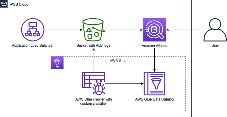
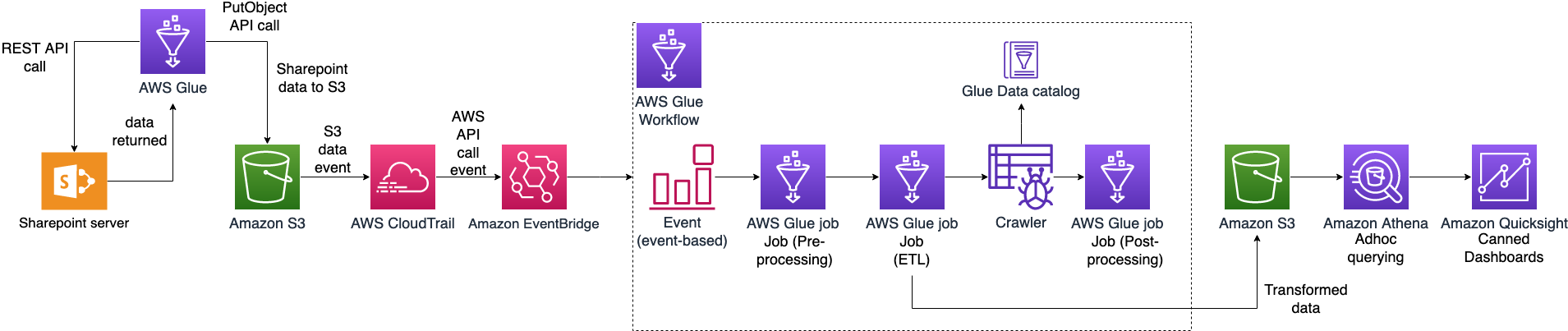
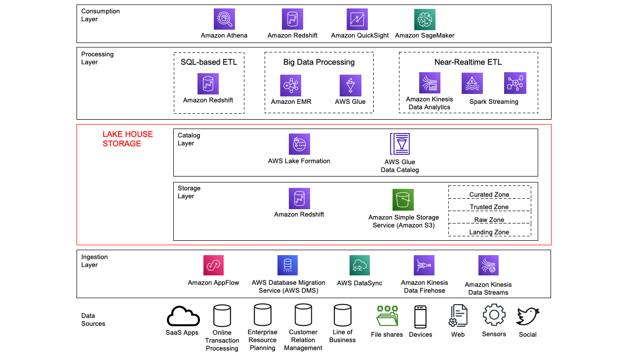
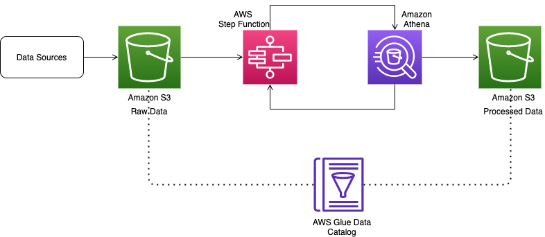
Figure 1 shows the flow of events and a high-level architecture diagram of the solution.
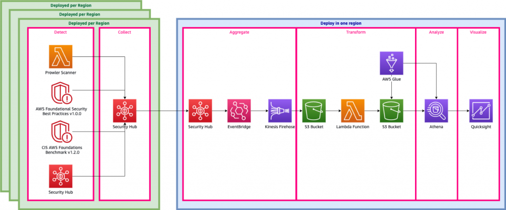
Figure 1. High level architecture diagram
The steps shown in Figure 1 include:
- Detect
- Collect
- Aggregate
- Transform
- Analyze
- Visualize
Detect
AWS offers a number of tools to help detect security findings continuously. These tools fall into three types:
In this blog, you will use two built-in security standards of Security Hub—CIS AWS Foundations Benchmark controls and AWS Foundational Security Best Practices Standard—and a serverless Prowler scanner that acts as a third-party partner product. In cases where AWS Organizations is used, member accounts send these findings to the member account’s Security Hub
Collect
Within a region, security findings are centralized into a single administrator account using Security Hub.
Aggregate
Using the cross-Region aggregation feature within Security Hub, findings within each administrator account can be aggregated and continuously synchronized across multiple regions.
Ingest
Security Hub not only provides a comprehensive view of security alerts and security posture across your AWS accounts, it also acts as a data sink for your security tools. Any tool that can expose data via AWS Security Finding Format (ASFF) can use the BatchImportFindings API action to push data to Security Hub. For more details, see Using custom product integration to send findings to AWS Security Hub and Available AWS service integrations in the Security Hub User Guide.
Transform
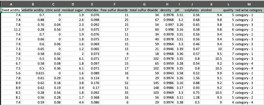
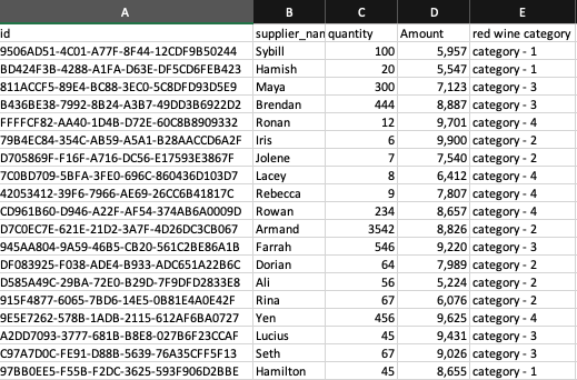
Data coming out of Security Hub is exposed via Amazon EventBridge. Unfortunately, it’s not quite in a form that Athena can consume. EventBridge streams data through Amazon Kinesis Data Firehose directly to Amazon Simple Storage Service (Amazon S3). From Amazon S3, you can create an AWS Lambda function that flattens and fixes some of the column names, such as by removing special characters that Athena cannot recognize. The Lambda function then saves the results back to S3. Finally, an AWS Glue crawler dynamically discovers the schema of the data and creates or updates an Athena table.
Analyze
You will aggregate the raw findings data and create metrics along various grains or pivots by creating a simple yet meaningful Athena view. With Athena, you also can use views to join the data with other data sources, such as your organization’s configuration management database (CMDB) or IT service management (ITSM) system.
Visualize
Using QuickSight, you will register the data sources and build visualizations that can be used to identify areas where security can be improved or reduce risk. This post shares steps detailing how to do this in the Build QuickSight visualizations section below.
Use AWS CDK to deploy the infrastructure
In order to analyze and visualize security related findings, you will need to deploy the infrastructure required to detect, ingest, and transform those findings. You will use an AWS CDK stack to deploy the infrastructure to your account. To begin, review the prerequisites to make sure you have everything you need to deploy the CDK stack. Once the CDK stack is deployed, you can deploy the actual infrastructure. After the infrastructure has been deployed, you will build an Athena view and a QuickSight visualization.
Install the software to deploy the solution
For the solution in this blog post, you must have the following tools installed:
- The solution in this blog post is written in Python, so you must install Python in addition to CDK. Instructions on how to install Python version 3.X can be found on their downloads page.
- AWS CDK requires node.js. Directions on how to install node.js can found on the node.js downloads page.
- This CDK application uses Docker for local bundling. Directions for using Docker can be found at Get Docker.
- AWS CDK—a software-development framework for defining cloud infrastructure in code and provisioning it through AWS CloudFormation. To install CDK, visit AWS CDK Toolkit page.
To confirm you have the everything you need
- Confirm you are running version 1.108.0 or later of CDK.
$ cdk ‐‐version
- Download the code from github by cloning the repository. cd into the clone directory.
$ git clone [email protected]:aws-samples/aws-security-hub-analytic-pipeline.git
$ cd aws-security-hub-analytic-pipeline
- Manually create a virtualenv.
$ python3 -m venv .venv
- After the initialization process completes and the virtualenv is created, you can use the following step to activate your virtualenv.
$ source .venv/bin/activate
- If you’re using a Windows platform, use the following command to activate virtualenv:
% .venv/Scripts/activate.bat
- Once the virtualenv is activated, you can install the required dependencies.
$ pip install -r requirements.txt
Use AWS CDK to deploy the infrastructure into your account
The following steps use AWS CDK to deploy the infrastructure. This infrastructure includes the various scanners, Security Hub, EventBridge, and Kinesis Firehose streams. When complete, the raw Security Hub data will already be stored in an S3 bucket.
To deploy the infrastructure using AWS CDK
- If you’ve never used AWS CDK in the account you’re using or if you’ve never used CDK in the us-east-1, us-east-2, or us-west-1 Regions, you must bootstrap the regions via the command prompt.
$ cdk bootstrap
- At this point, you can deploy the stack to your default AWS account via the command prompt.
$ cdk deploy –all
- While cdk deploy is running, you will see the output in Figure 2. This is a prompt to ensure you’re aware that you’re making a security-relevant change and creating AWS Identity and Access Management (IAM) roles. Enter y when prompted to continue the deployment process:

Figure 2. CDK approval prompt to create IAM roles
- Confirm cdk deploy is finished. When the deployment is finished, you should see three stack ARNs. It will look similar to Figure 3.
Figure 3. Final output of CDK deploy


As a result of the deployed CDK code, Security Hub and the Prowler scanner will automatically scan your account, process the data, and send it to S3. While it takes less than an hour for some data to be processed and searchable in Athena, we recommend waiting 24 hours before proceeding to the next steps, to ensure enough data is processed to generate useful visualizations. This is because the remaining steps roll-up findings by the hour. Also, it takes several minutes to get initial results from the Security Hub standards and up to an hour to get initial results from Prowler.
Build an Athena view
Now that you’re deployed the infrastructure to detect, ingest, and transform security related findings, it’s time to use an Athena view to accomplish the analyze portion of the solution. The following view aggregates the number of findings for a given day. Athena views can be used to summarize data or enrich it with data from other sources. Use the following steps to build a simple example view. For more information on creating Athena views, see Working with Views.
To build an Athena view
- Open the AWS Management Console and ensure that the Region is set to us-east-1 (Northern Virginia).
- Navigate to the Athena service. If you’ve never used this service, choose Get Started to navigate to the Query Editor screen. Otherwise, the Query Editor screen is the default view.
- If you’re new to Athena, you also need to set up a query result location.
- Choose Settings in the top right of the Query Editor screen to open the settings panel.
- Choose Select to select a query result location.

Figure 4. Athena settings
- Locate an S3 bucket in the list that starts with analyticsink-queryresults and choose the right-arrow icon.
- Choose Select to select a query results bucket.

Figure 5. Select S3 location confirmation
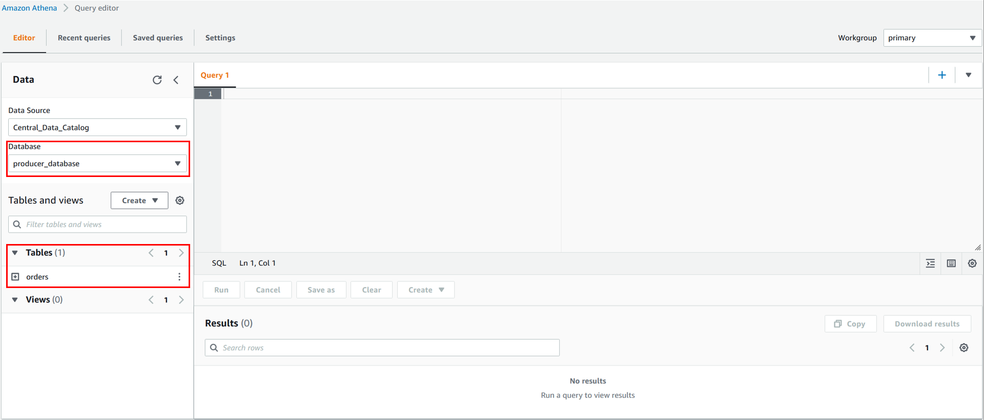
- Select AwsDataCatalog as the Data source and security_hub_database as the Database. The Query Editor screen should look like Figure 6.

Figure 6. Empty query editor
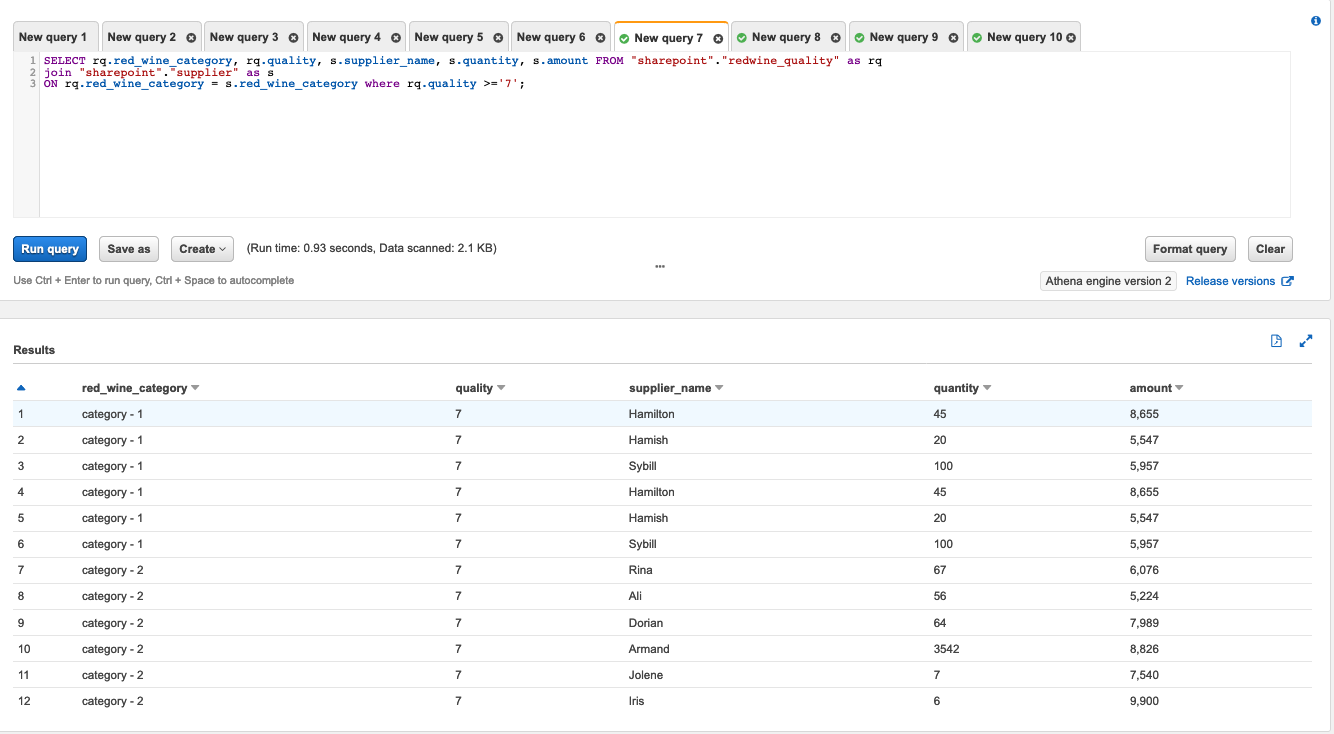
- Copy and paste the following SQL in the query window:
CREATE OR REPLACE VIEW “security-hub-rolled-up-finding” AS
SELECT
“date_format”(“from_iso8601_timestamp”(updatedat), ‘%Y-%m-%d %H:00’) year_month_day
, region
, compliance_status
, workflowstate
, severity_label
, COUNT(DISTINCT title) as cnt
FROM
security_hub_database.“security-hub-crawled-findings”
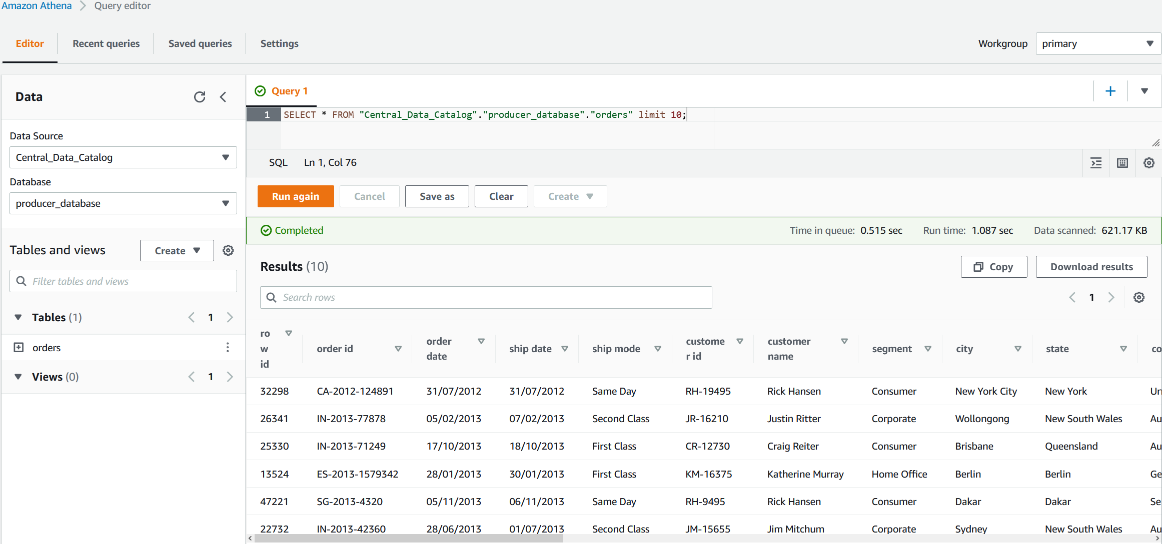
GROUP BY “date_format”(“from_iso8601_timestamp”(updatedat), ‘%Y-%m-%d %H:00’), compliance_status, workflowstate, severity_label, region - Choose the Run query button.


If everything is correct, you should see Query successful in the Results, as shown in Figure 7.
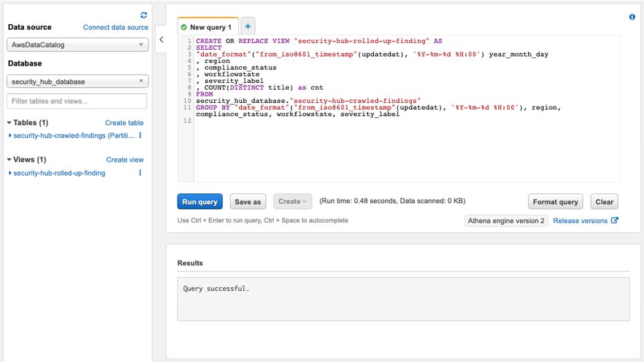
Figure 7. Creating an Athena view
Build QuickSight visualizations
Now that you’ve deployed the infrastructure to detect, ingest, and transform security related findings, and have created an Athena view to analyze those findings, it’s time to use QuickSight to visualize the findings. To use QuickSight, you must first grant QuickSight permissions to access S3 and Athena. Next you create a QuickSight data source. Third, you will create a QuickSight analysis. (Optional) When complete, you can publish the analysis.
You will build a simple visualization that shows counts of findings over time separated by severity, though it’s also possible to use QuickSight to tell rich and compelling visual stories.
In order to use QuickSight, you need to sign up for a QuickSight subscription. Steps to do so can be found in Signing Up for an Amazon QuickSight Subscription.
The first thing you need to do once logged in to QuickSight is create the data source. If this is your first time logging in to the service, you will be greeted with an initial QuickSight page as shown in Figure 8.
Figure 8. Initial QuickSight page
Grant QuickSight access to S3 and Athena
While creating the Athena data source will enable QuickSight to query data from Athena, you also need to enable QuickSight to read from S3.
To grant QuickSight access to S3 and Athena
- Inside QuickSight, select your profile name (upper right). Choose Manage QuickSight, and then choose Security & permissions.
- Choose Add or remove.
- Ensure the checkbox next to Athena is selected.
- Ensure the checkbox next to Amazon S3 is selected.
- Choose Details and then choose Select S3 Buckets.
- Locate an S3 bucket in the list that starts with analyticsink-bucket and ensure the checkbox is selected.

Figure 9. Example permissions
- Choose Finish to save changes.

Create a QuickSight dataset
Once you’ve given QuickSight the necessary permissions, you can create a new dataset.
To create a QuickSight dataset
- Choose Datasets from the navigation pane at left. Then choose New Dataset.
Figure 10. Dataset page
- To create a new Athena connection profile, use the following steps:
- In the FROM NEW DATA SOURCES section, choose the Athena data source card.
- For Data source name, enter a descriptive name. For example: security-hub-rolled-up-finding.
- For Athena workgroup choose [ primary ].
- Choose Validate connection to test the connection. This also confirms encryption at rest.
- Choose Create data source.
- On the Choose your table screen, select:
Catalog: AwsDataCatalog
Database: security_hub_database
Table: security-hub-rolled-up-finding - Finally, select the Import to SPICE for quicker analytics option and choose Visualize.

Once you’re finished, the page to create your first analysis will automatically open. Figure 11 shows an example of the page.
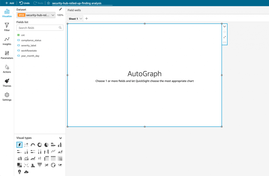
Figure 11. Create an analysis page
Create a QuickSight analysis
A QuickSight analysis is more than just a visualization—it helps you uncover hidden insights and trends in your data, identify key drivers, and forecast business metrics. You can create rich analytic experiences with QuickSight. For more information, visit Working with Visuals in the QuickSight User Guide.
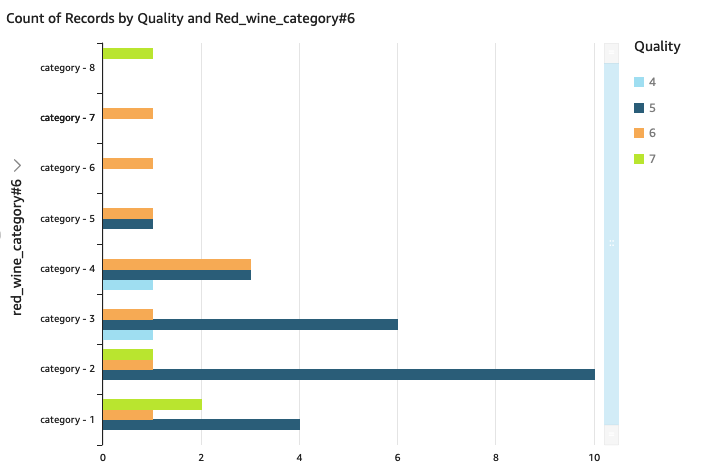
For simplicity, you’ll build a visualization that summarizes findings categories by severity and aggregated by hour.
To create a QuickSight analysis
- Choose Line Chart from the Visual Types.

Figure 12. Visual types
- Select Fields. Figure 13 shows what your field wells should look like at the end of this step.
- Locate the year_month_day_hour field in the field list and drag it over to the X axis field well.
- Locate the cnt field in the field list and drag it over to the Value field well.
- Locate the severity_label field in the field list and drag it over to Color field well.

Figure 13. Field wells
- Add Filters.
- Select Filter in the left navigation panel.

Figure 14. Filters panel
- Choose Create one… and select the compliance_status field.
- Expand the filter and clear NOT_AVAILABLE and PASSED (Note: depending on your data, you might not have all of these statuses).
- Choose Apply to apply the filter.

Figure 15. Filtering out findings that are not failing
- Select Filter in the left navigation panel.


You should now see a visualization that looks like Figure 16, which shows a summary count of events and their severity.
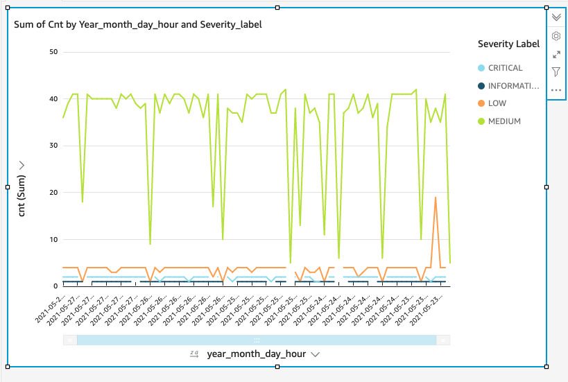
Figure 16. Example visualization (note: this visualization has five days’ worth of data.)
Publish a QuickSight analysis dashboard (optional)
Publishing a dashboard is a great way to share reports with leaders. This two-step process allows you to share visualizations as a dashboard.
To publish a QuickSight analysis
- Choose Share on the application bar, then choose Publish dashboard.
- Select Publish new dashboard as, and then enter a dashboard name, such as Security Hub Findings by Severity.
You can also embed dashboards into web applications. This requires using the AWS SDK or through the AWS Command Line Interface (AWS CLI). For more information, see Embedding QuickSight Data Dashboards for Everyone.
Encouraged security posture in QuickSight
QuickSight has a number of security features. While the AWS Security section of the QuickSight User Guide goes into detail, here’s a summary of the standards that apply to this specific scenario. For more details see AWS security in Amazon QuickSight within the QuickSight user guide.
Clean up (optional)
When done, you can clean up QuickSight by removing the Athena view and the CDK stack. Follow the detailed steps below to clean up everything.
To clean up QuickSight
- Open the console and choose Datasets in the left navigation pane.
- Select security-hub-rolled-up-finding then choose Delete dataset.
- Confirm dataset deletion by choosing Delete.
- Choose Analyses from the left navigation pane.
- Choose the menu in the lower right corner of the security-hub-rolled-up-finding card.

Figure 17. Example analysis card
- Select Delete and confirm Delete.

To remove the Athena view
- Paste the following SQL in the query window:
DROP VIEW “security-hub-rolled-up-finding”
- Choose the Run query button.
To remove the CDK stack
- Run the following command in your terminal:
cdk destroy
Note: If you experience errors, you might need to reactivate your Python virtual environment by completing steps 3–5 of Use AWS CDK to deploy the infrastructure.
Conclusion
In this blog, you used Security Hub and QuickSight to deploy a scalable analytic pipeline for your security tools. Security Hub allowed you to join and collect security findings from multiple sources. With QuickSight, you summarized data for your senior leaders and decision-makers to give them the right data in real-time.
You ensured that your sensitive data remained protected by explicitly granting QuickSight the ability to read from a specific S3 bucket. By authorizing access only to the data sources needed to visualize your data, you ensure least privilege access. QuickSight supports many other AWS data sources, including Amazon RDS, Amazon Redshift, Lake Formation, and Amazon OpenSearch Service (successor to Amazon Elasticsearch Service). Because the data doesn’t live inside an Amazon Virtual Private Cloud (Amazon VPC), you didn’t need to grant access to any specific VPCs. Limiting access to VPCs is another great way to improve the security of your environment.
If you have feedback about this post, submit comments in the Comments section below. If you have questions about this post, start a new thread on the Security Hub forum. To start your 30-day free trial of Security Hub, visit AWS Security Hub.
Want more AWS Security how-to content, news, and feature announcements? Follow us on Twitter.


 Once you create the data source Quicksight lists all the views and tables available under the specified database (in our case it is:- due_eventdb). Select the email_all_events view as data source.
 Select the event data location for analysis. There are mainly two options available which are a/ Import to Spice quicker analysis b/ Directly query your data. Please select the preferred options and then click on “visualize the data”.
 Now that you have selected a data source, you will be taken to a blank quick sight canvas (Blank analysis page) as shown in the following Image, please drag and drop what
  As part of this blog, we have displayed how to create some simple analysis graphs to visualize the engagement events.
 Select all the event dimensions that you want to put it as part of the Table in X axis. Amazon Quicksight table can be extended to show as many as tables columns, this completely depends upon the business requirement how much data marketers want to visualize.
 To create a Quicksight dashboards from the Quicksight analysis click Share menu option at the top right corner then select publish dashboard”. Provide required dashboard name while publishing the dashboard”. Same dashboard can be shared with multiple audiences in the Organization.
 Following is the final version of the dashboard. As mentioned above Quicksight dashboards can be shared with other stakeholders and also complete dashboard can be exported as excel sheet.


 Lotfi is a Senior Solutions Architect working for the Public Sector team with Amazon Web Services. He helps public sector customers across EMEA realize their ideas, build new services, and innovate for citizens. In his spare time, Lotfi enjoys cycling and running.


