Post Syndicated from Jignesh Gohel original https://aws.amazon.com/blogs/big-data/create-amazon-s3-storage-lens-metrics-dashboard-amazon-quicksight/
Companies use Amazon Simple Storage Service (Amazon S3) for its flexibility, durability, scalability, and ability to perform many things besides storing data. This has led to an exponential rise in the usage of S3 buckets across numerous AWS Regions, across tens or even hundreds of AWS accounts. To optimize costs and analyze security posture, Amazon S3 Storage Lens provides a single view of object storage usage and activity across your entire Amazon S3 storage. S3 Storage Lens includes an embedded dashboard to understand, analyze, and optimize storage with over 29 usage and activity metrics, aggregated for your entire organization, with drill-downs for specific accounts, Regions, buckets, or prefixes. In addition to being accessible in a dashboard on the Amazon S3 console, the raw data can also be scheduled for export to an S3 bucket.
For most customers, the S3 Storage Lens dashboard will cover all your needs. However, you may require specialized views of your S3 Storage Lens metrics, including combining data across multiple AWS accounts, or with external data sources. For such cases, you can use Amazon QuickSight, which is a scalable, serverless, embeddable, machine learning (ML)-powered business intelligence (BI) service built for the cloud. QuickSight lets you easily create and publish interactive BI dashboards that include ML-powered insights.
In this post, you learn how to use QuickSight to create simple customized dashboards to visualize S3 Storage Lens metrics. Specifically, this solution demonstrates two customization options:
- Combining S3 Storage Lens metrics with external sources and being able to filter and visualize the metrics based on one or multiple accounts
- Restricting users to view Amazon S3 metrics data only for specific accounts
You can further customize these dashboards based on your needs.
Solution architecture
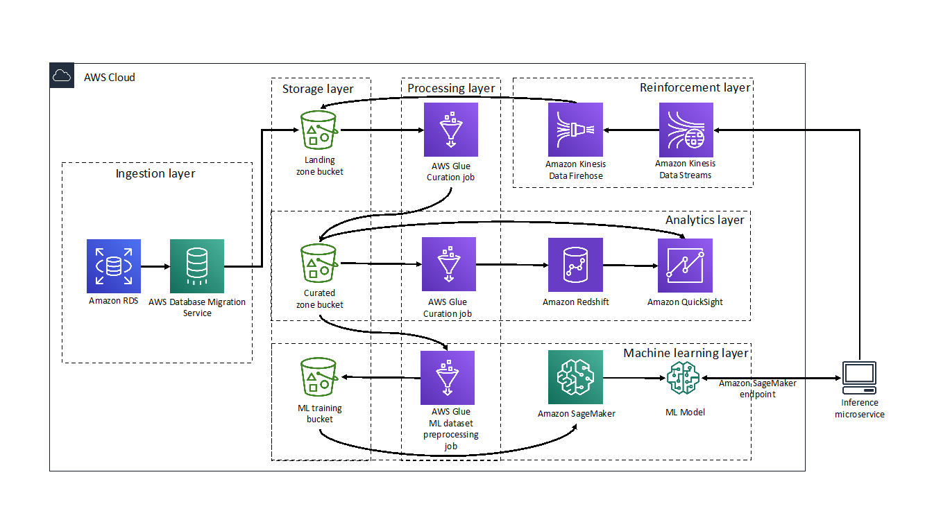
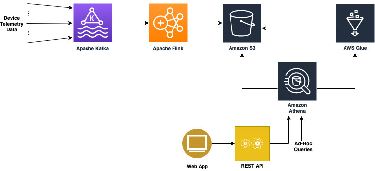
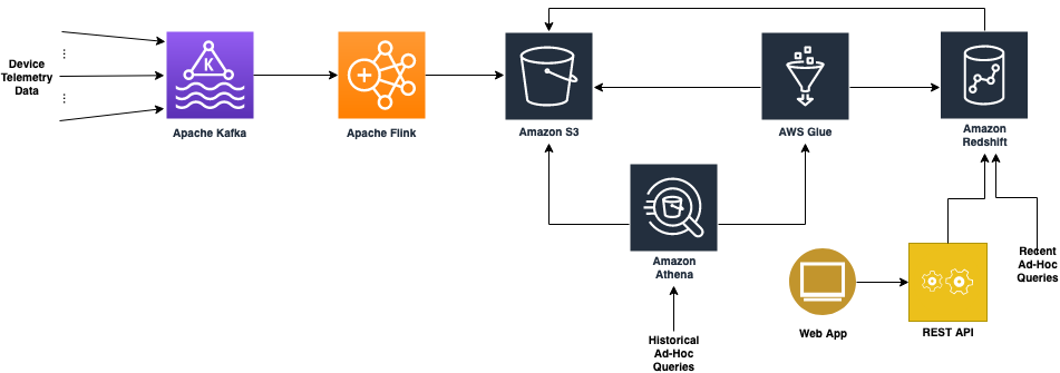
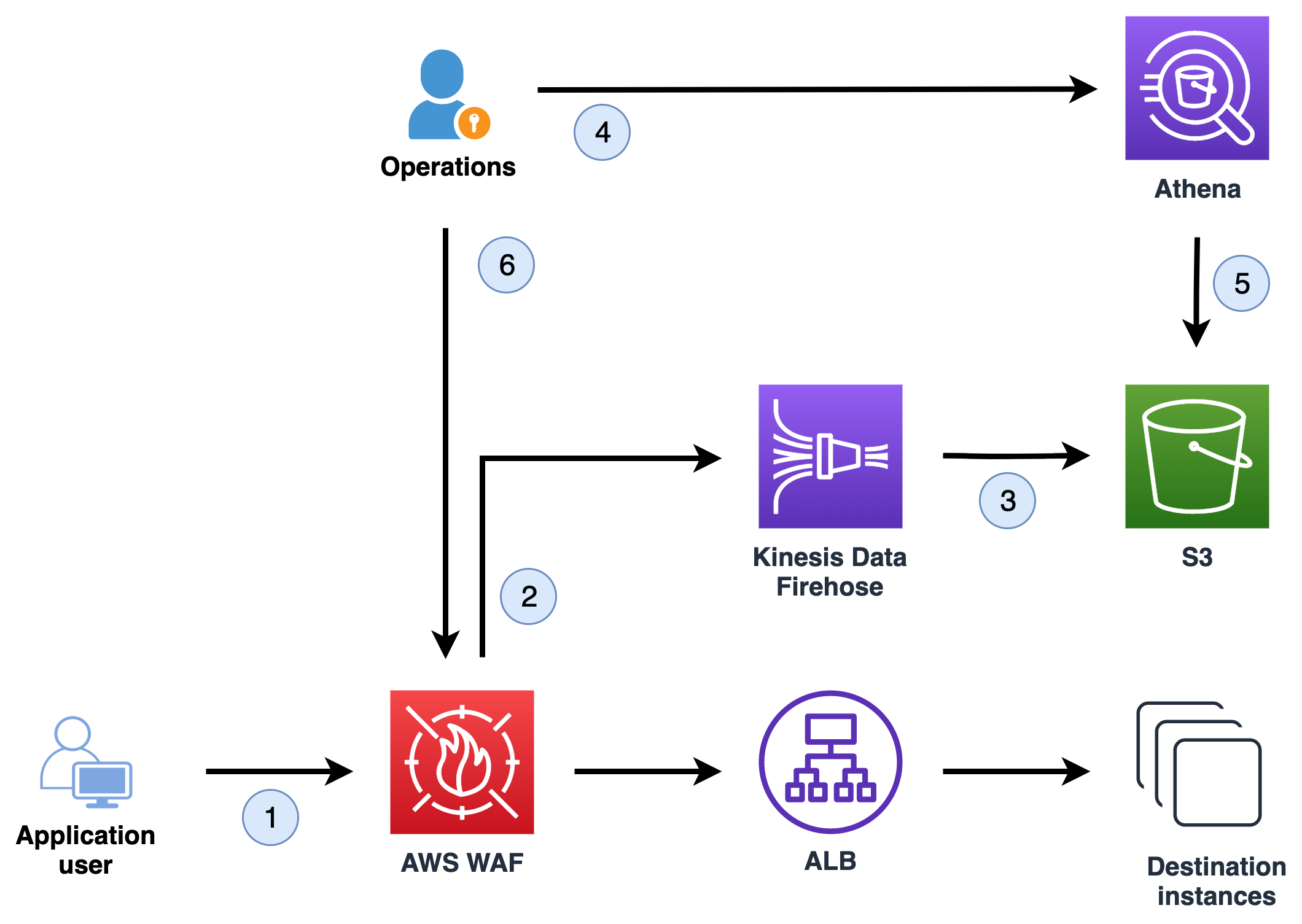
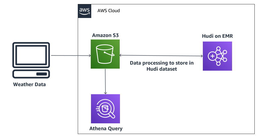
The following diagram shows the high-level architecture of this solution. In addition to S3 Storage Lens and QuickSight, we use other AWS Serverless services like AWS Glue and Amazon Athena.
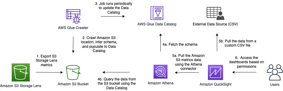
The data flow includes the following steps:
- S3 Storage Lens collects the S3 metrics and exports them daily to a user-defined S3 bucket. Note that first we need to activate S3 Storage Lens from the Amazon S3 console and configure it to export the file either in CSV or Apache Parquet format.
- An AWS Glue crawler scans the data from the S3 bucket and populates the AWS Glue Data Catalog with tables. It automatically infers schema, format, and data types from the S3 bucket.
- You can schedule the crawler to run at regular intervals to keep metadata, table definitions, and schemas in sync with data in the S3 bucket. It automatically detects new partitions in Amazon S3 and adds the partition’s metadata to the AWS Glue table.
- Athena performs the following actions:
- Uses the table populated by the crawler in Data Catalog to fetch the schema.
- Queries and analyzes the data in Amazon S3 directly using standard SQL.
- QuickSight performs the following actions:
- Uses the Athena connector to import the Amazon S3 metrics data.
- Fetches the external data from a custom CSV file.
To demonstrate this, we have a sample CSV file that contains the mapping of AWS account numbers to team names owning these accounts. QuickSight combines these datasets using the data source join feature.
- When the combined data is available in QuickSight, users can create custom analysis and dashboards, apply appropriate QuickSight permissions, and share dashboards with other users.
At a high level, this solution requires you to complete the following steps:
- Enable S3 Storage Lens in your organization’s payer account or designate a member account. For instructions to have a member account as a delegated administrator, see Enabling a delegated administrator account for Amazon S3 Storage Lens.
- Set up an AWS Glue crawler, which populates the Data Catalog to query S3 Storage Lens data using Athena.
- Use QuickSight to import data (using the Athena connector) and create custom visualizations and dashboards that can be shared across multiple QuickSight users or groups.
Enable and configure the S3 Storage Lens dashboard
S3 Storage Lens includes an interactive dashboard available on the Amazon S3 console. It shows organization-wide visibility into object storage usage, activity trends, and makes actionable recommendations to improve cost-efficiency and apply data protection best practices. First you need to activate S3 Storage Lens via the Amazon S3 console. After it’s enabled, you can access an interactive dashboard containing preconfigured views to visualize storage usage and activity trends, with contextual recommendations. Most importantly, it also provides the ability to export metrics in CSV or Parquet format to an S3 bucket of your choice for further use. We use this export metrics feature in our solution. The following steps provide details on how you can enable this feature in your account.
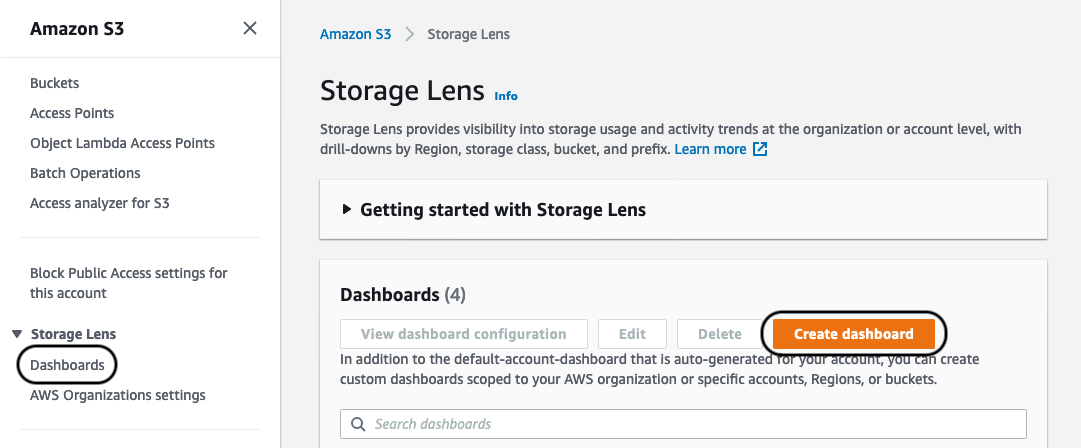
- On the Amazon S3 console, under Storage Lens in the navigation pane, choose Dashboards.
- Choose Create dashboard.
- Provide the appropriate details in the Create dashboard
- Make sure to select Include all accounts in your organization, Include Regions, and Include all Regions.

S3 Storage Lens has two tiers: Free metrics, which is free of charge, automatically available for all Amazon S3 customers, and contains 15 usage-related metrics; and Advanced metrics and recommendations, which has an additional charge, but includes all 29 usage and activity metrics with 15-month data retention, and contextual recommendations. For this solution, we select Free metrics. If you need additional metrics, you may select Advanced metrics.
- For Metrics export, select Enable.
- For Choose and output format, select Apache Parquet.
- For Destination bucket, select This account.
- For Destination, enter your S3 bucket path.

We highly recommend following security best practices for the S3 bucket you use, along with server-side encryption available with export. You can use an Amazon S3 key (SSE-S3) or AWS Key Management Service key (SSE-KMS) as encryption key types.
- Choose Create dashboard.
The data population process can take up to 48 hours. Proceed to the next steps only after the dashboard is available.
Set up the AWS Glue crawler
AWS Glue is serverless, fully managed extract, transform, and load (ETL) service that makes it simple and cost-effective to categorize your data, clean it, enrich it, and move it reliably between various data stores and data streams. AWS Glue consists of a central metadata repository known as the AWS Glue Data Catalog, an ETL engine, and a flexible scheduler that handles dependency resolution, job monitoring, and retries. We can use the AWS Glue to discover data, transform it, and make it available for search and querying. The AWS Glue Data Catalog is an index to the location, schema, and runtime metrics of your data. Athena uses this metadata definition to query data available in Amazon S3 using simple SQL statements.
The AWS Glue crawler populates the Data Catalog with tables from various sources, including Amazon S3. When the crawler runs, it classifies data to determine the format, schema, and associated properties of the raw data, performs grouping of data into tables or partitions, and writes metadata to the Data Catalog. You can configure the crawler to run at specific intervals to make sure the Data Catalog is in sync with the underlying source data.
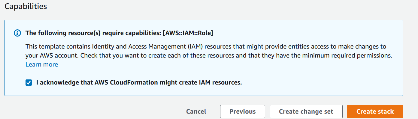
For our solution, we use these services to catalog and query exported S3 Storage Lens metrics data. First, we create the crawler via the AWS Glue console. For the purpose of this example, we provide an AWS CloudFormation template that deploys the required AWS resources. This template creates the CloudFormation stack with three AWS resources in your AWS account:
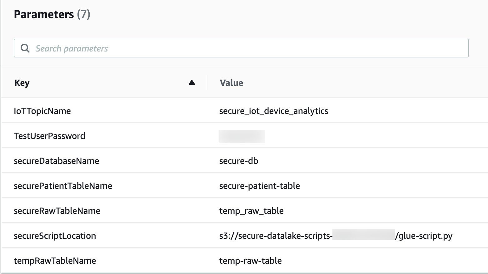
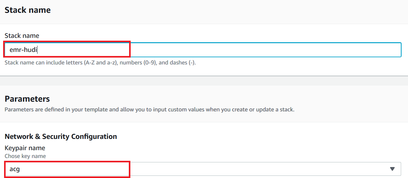
When you create your stack with the CloudFormation template, provide the following information:
- AWS Glue database name
- AWS Glue crawler name
- S3 URL path pointing to the
reportsfolder where S3 Storage Lens has exported metrics data. For example,s3://[Name of the bucket]/StorageLens/o-lcpjprs6wq/s3-storage-lense-parquet-v1/V_1/reports/.
After the stack is complete, navigate to the AWS Glue console and confirm that a new crawler job is listed on the Crawlers page. When the crawler runs for the first time, it creates the table reports in the Data Catalog. The Data Catalog may need to be periodically refreshed, so this job is configured to run every day at midnight to sync the data. You can change this configuration to your desired schedule.
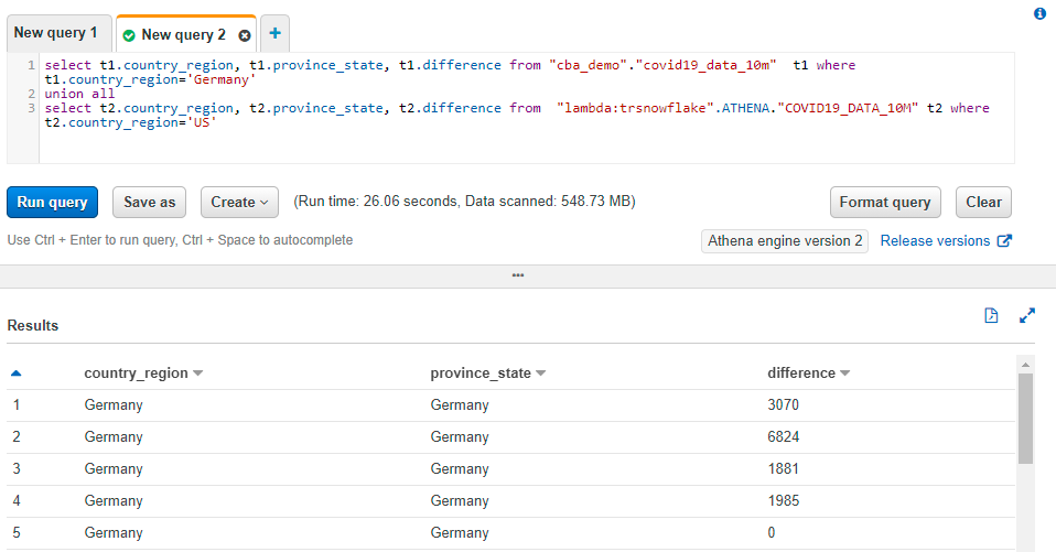
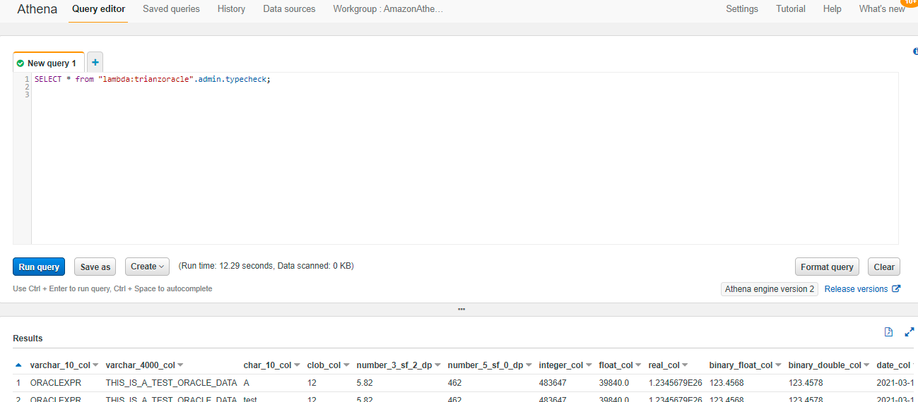
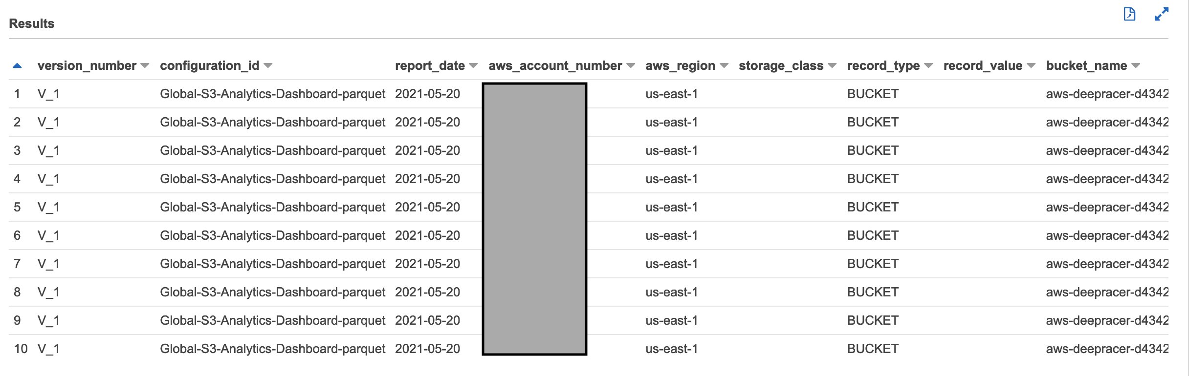
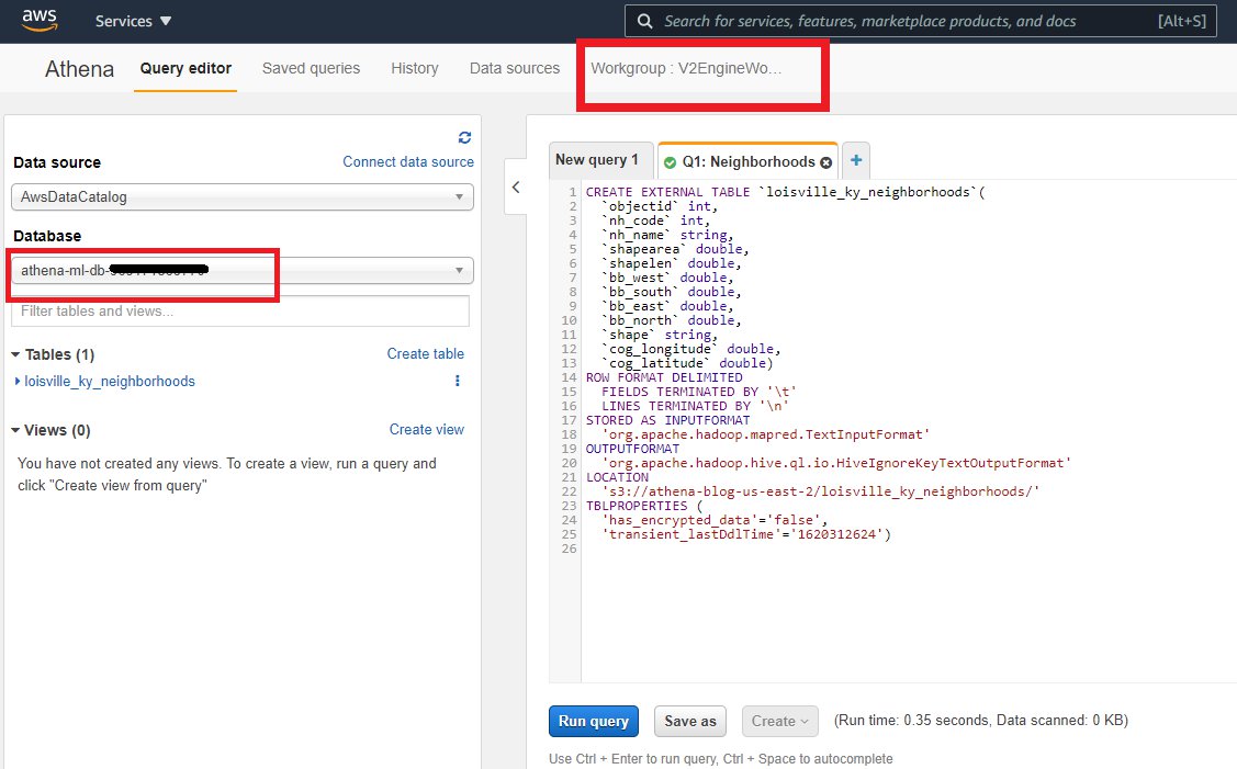
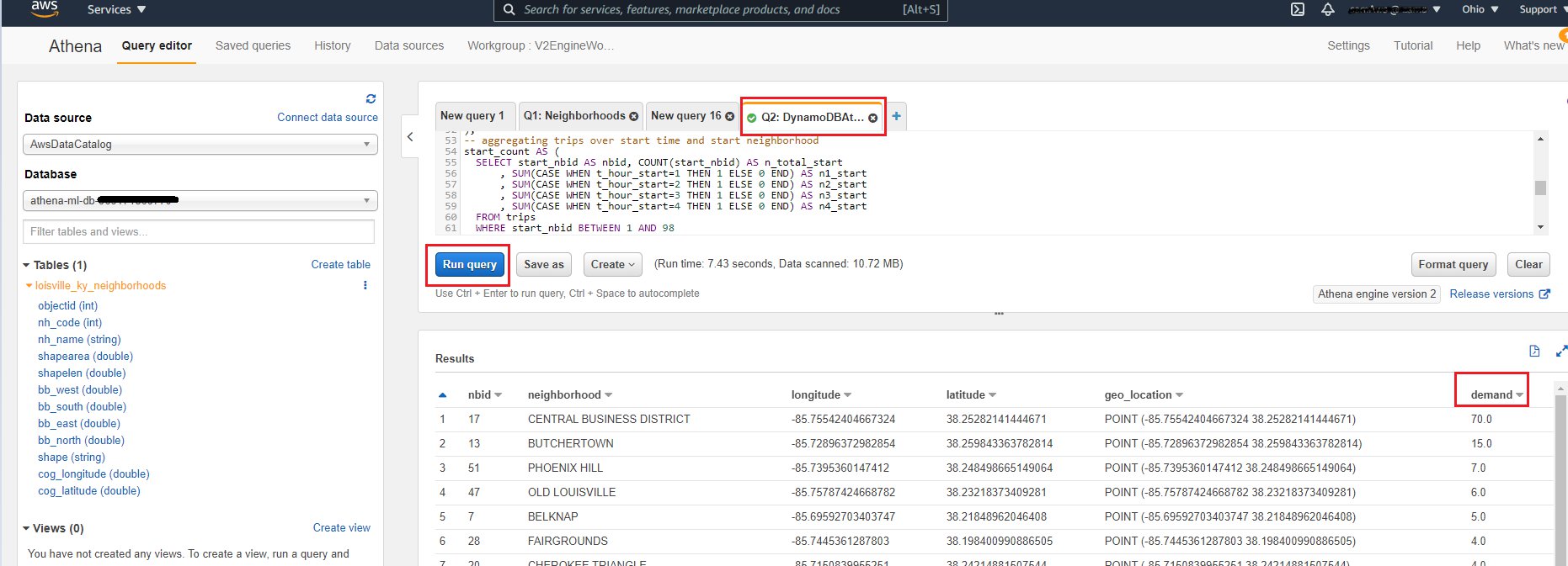
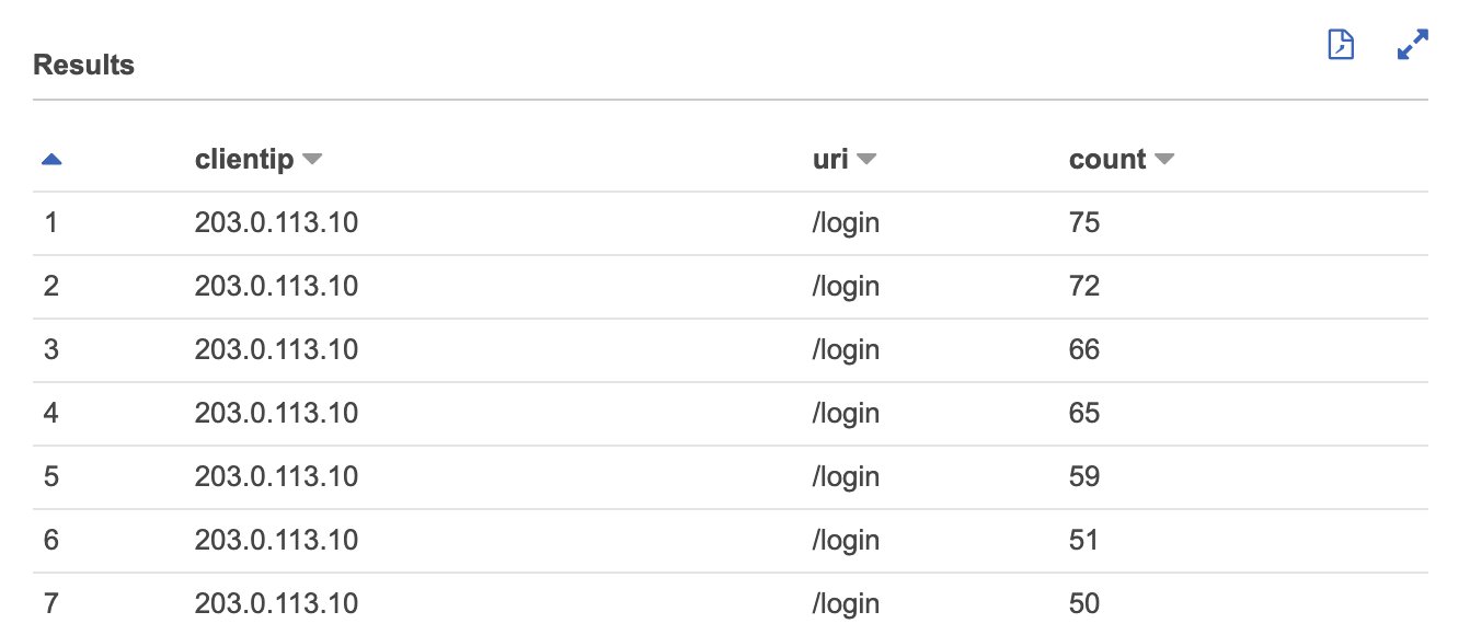
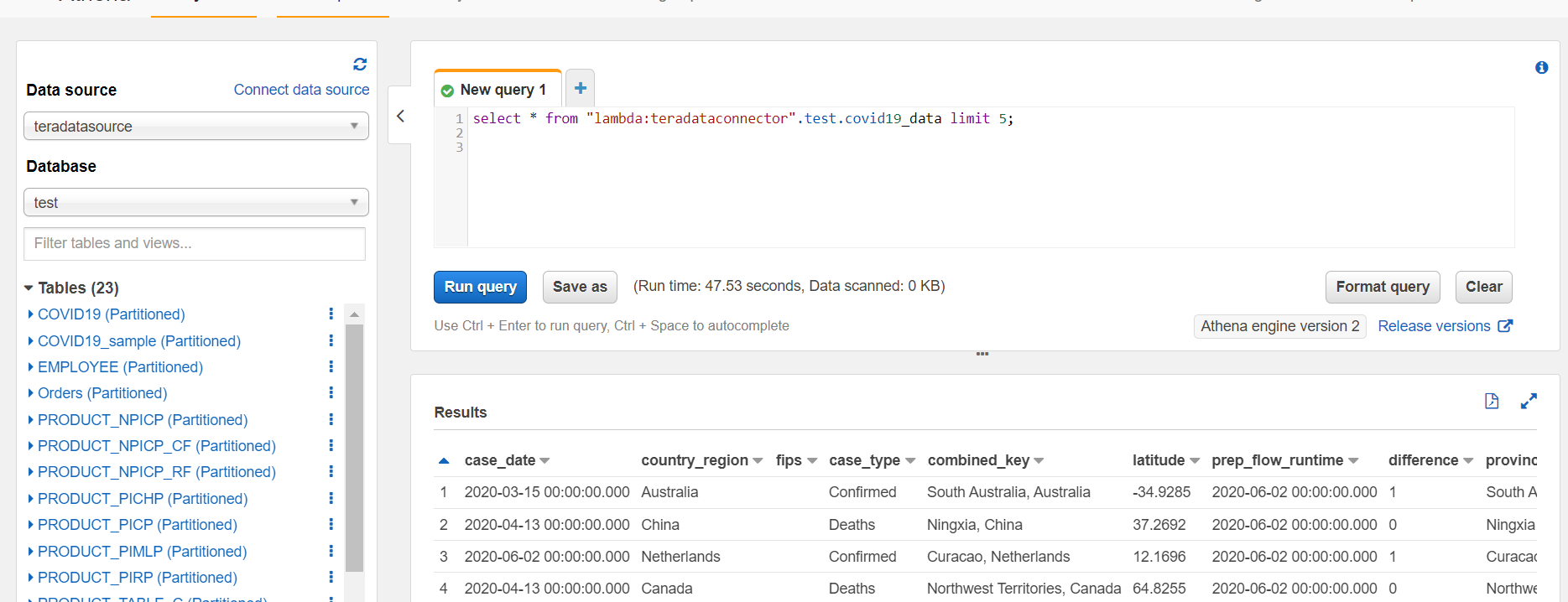
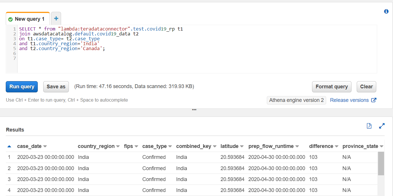
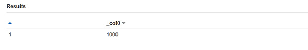
After the crawler job runs, we can confirm that the data is accessible using the following query in Athena (make sure to run this query in the database provided in the CloudFormation template):
Running this query should return results similar to the following screenshot.
Create a QuickSight dashboard
When the data is available to access using Athena, we can use QuickSight to create customized analytics and publish dashboards across multiple users. This process involves creating a new QuickSight dataset, creating the analysis using this dataset, creating the dashboard, and configuring user permissions and security.
To get started, you must be signed in to QuickSight using the same payer account. If you’re signing into QuickSight for the first time, you’re prompted to complete the initial signup process (for example, choosing QuickSight Enterprise Edition). You’re also required to provide QuickSight access to your S3 bucket and Athena. For instructions on adding permissions, see Insufficient Permissions When Using Athena with Amazon QuickSight.
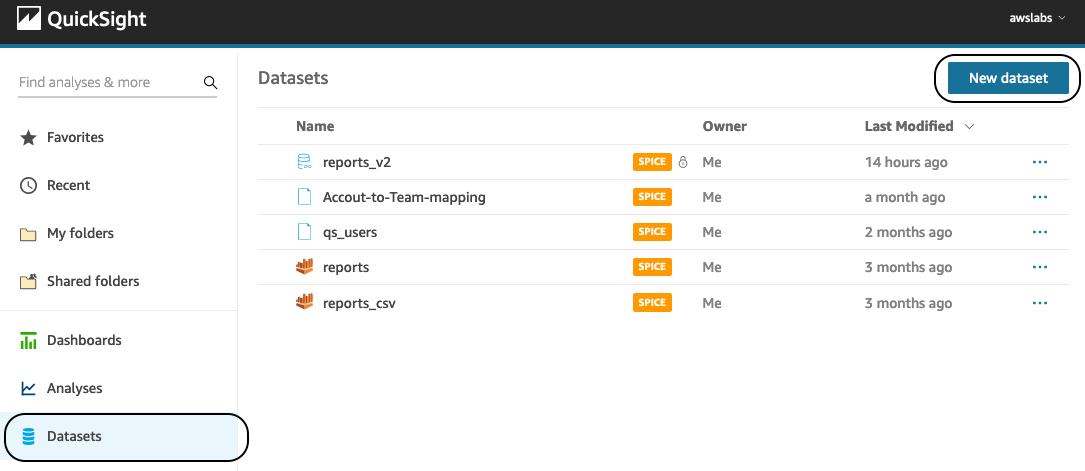
- In the QuickSight navigation pane, choose Datasets.
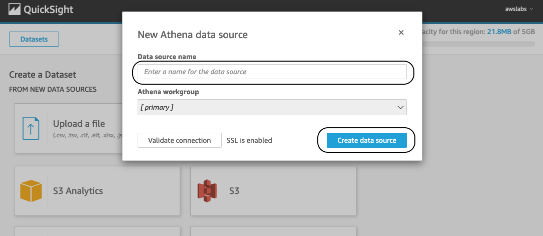
- Choose New dataset and select Athena.
- For Data source name, enter a name.
- Choose Create data source.
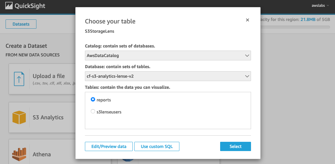
- For Catalog, choose AwsDataCatalog.
- For Database, choose the AWS Glue database that contains the table for S3 Storage Lens.
- For Tables, select your table (for this post,
reports).
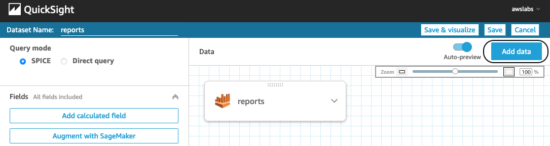
- Choose Edit dataset and choose the query mode SPICE.
- Change the format of
report_dateanddtto Date. - Choose Save.
We can use the cross data source join feature in QuickSight to connect external data sources to the S3 Storage Lens dataset. For this example, let’s say we want to visualize the number of S3 buckets mapped to the internal teams. This data is external to S3 Storage Lens and stored in a CSV file, which contains the mapping between the account numbers and internal team names.

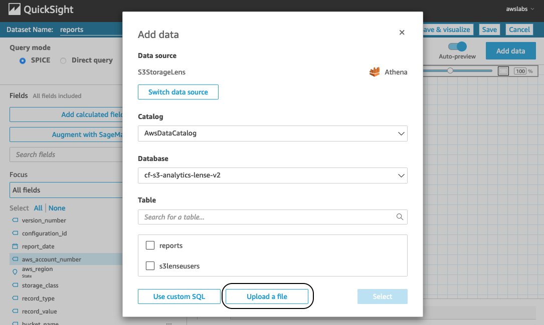
- To import this data into our existing dataset, choose Add data.
- Choose Upload a file to import the CSV file to the dataset.
We’re redirected to the join configuration screen. From here, we can configure the join type and join clauses to connect these two data sources. For more information about the cross data source join functionality, see Joining across data sources on Amazon QuickSight.
- For this example, we need to perform the left join on
columns aws_account_number(from thereportstable) andAccount(from theAccount-to-Team-mappingtable). This left join returns all records from thereportstable and matching records fromAccount-to-Team-mapping. - Choose Apply after selecting this configuration.
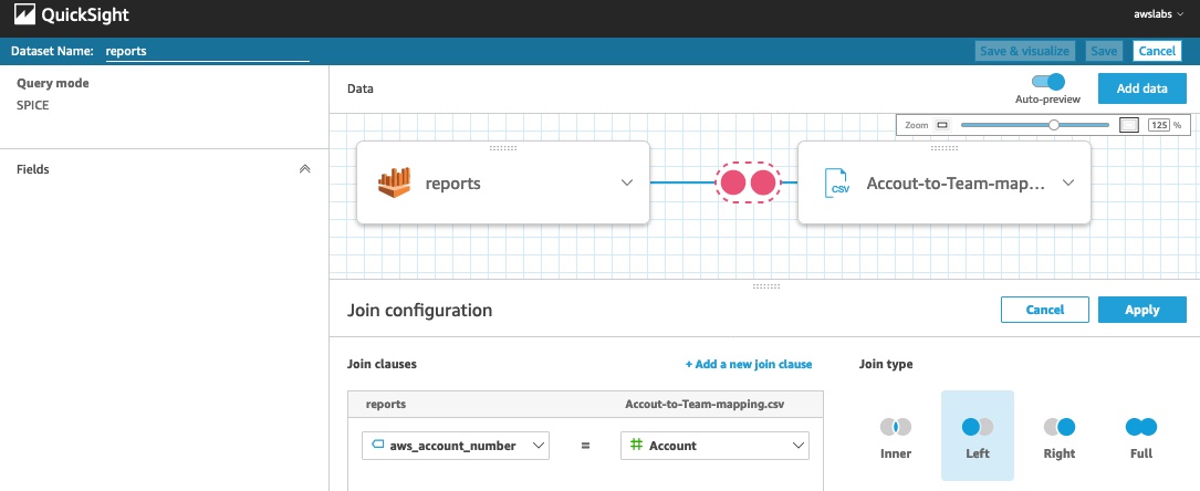
- Choose Save & visualize.
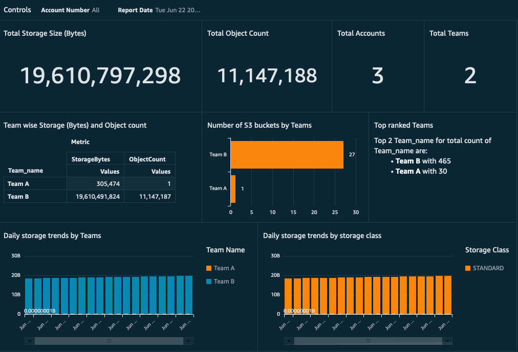
From here, you can create various analyses and visualizations on the imported datasets. For instructions on creating visualizations, see Creating an Amazon QuickSight Visual. We provide a sample template you can use to get the basic dashboard. This dashboard provides metrics for total Amazon S3 storage size, object count, S3 bucket by internal team, and more. It also allows authorized users to filter the metrics based on accounts and report dates. This is a simple report that can be further customized based on your needs.
S3 Storage Lens’s IAM security policies don’t apply to imported data into QuickSight. So before you share this dashboard with anyone, one might want to restrict access according to the security requirement and business role of the user. For a comprehensive set of security features, see AWS Security in Amazon QuickSight. For implementation examples, see Applying row-level and column-level security on Amazon QuickSight dashboards. In our example, instead of all users having access to view S3 Storage Lens data for all accounts, you might want to restrict user access to only specific accounts.
QuickSight provides a feature called row-level security that can restrict user access to only a subset of table rows (or records). You can base the selection of these subsets of rows on filter conditions defined on specific columns.
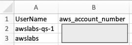
For our current example, we want to allow user access to view the Amazon S3 metrics dashboard only for a few accounts. For this, we can use the column aws_account_number as filter criteria with account number values. We can implement this by creating a CSV file with columns named UserName and aws_account_number, and adding the rows for users and a list of account numbers (comma-separated). In the following example file, we have added a sample value for the user awslabs-qs-1 with a specific account. This means that user awslabs-qs-1 can only see the rows (or records) that match with the corresponding aws_account_number values specified in the permission CSV.
For instructions on applying a permission rule file, see Using Row-Level Security (RLS) to Restrict Access to a Dataset.
You can further customize this QuickSight analysis to produce additional visualizations, apply additional permissions, and publish it to enterprise users and groups with various levels of security.
Conclusion
Harnessing the knowledge of S3 Storage Lens metrics with other custom data enables you to discover anomalies and identify cost-efficiencies across accounts. In this post, we used serverless components to build a workflow to use this data for real-time visualization. You can use this workflow to scale up and design an enterprise-level solution with a multi-account strategy and control fine-grained access to its data using the QuickSight row-level security feature.
About the Authors
 Jignesh Gohel is a Technical Account Manager at AWS. In this role, he provides advocacy and strategic technical guidance to help plan and build solutions using best practices, and proactively keep customers’ AWS environments operationally healthy. He is passionate about building modular and scalable enterprise systems on AWS using serverless technologies. Besides work, Jignesh enjoys spending time with family and friends, traveling and exploring the latest technology trends.
 Suman Koduri is a Global Category Lead for Data & Analytics category in AWS Marketplace. He is focused towards business development activities to further expand the presence and success of Data & Analytics ISVs in AWS Marketplace. In this role, he leads the scaling, and evolution of new and existing ISVs, as well as field enablement and strategic customer advisement for the same. In his spare time, he loves running half marathon’s and riding his motorcycle.


 Armando Segnini is a Data Architect with AWS Professional Services. He spends his time building scalable big data and analytics solutions for AWS Enterprise and Strategic customers. Armando also loves to travel with his family all around the world and take pictures of the places he visits.
 Xavier Naunay is a Data Architect with AWS Professional Services. He is part of the AWS ProServe team, helping enterprise customers solve complex problems using AWS services. In his free time, he is either traveling or learning about technology and other cultures.
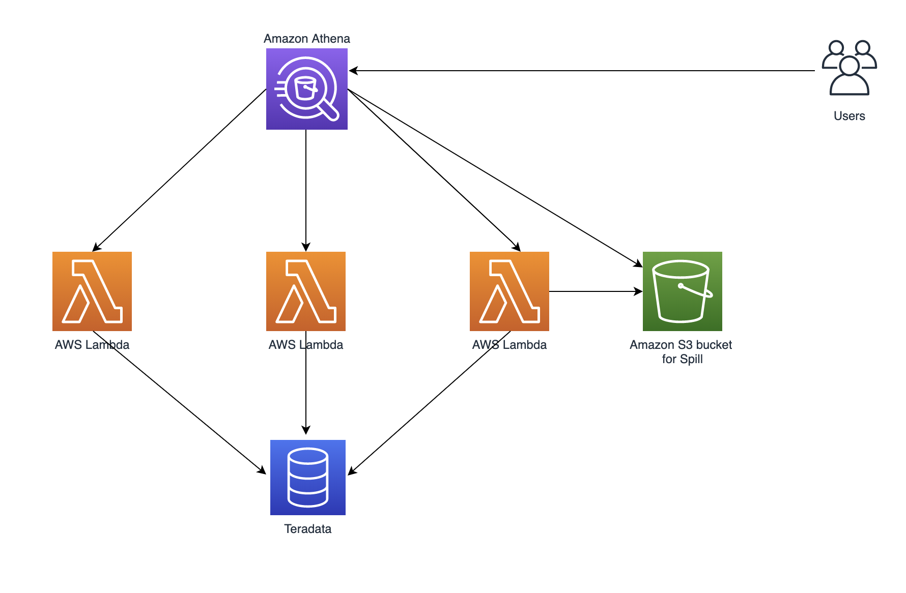


 Dhiraj Thakur is a Solutions Architect with Amazon Web Services. He works with AWS customers and partners to provide guidance on enterprise cloud adoption, migration and strategy. He is passionate about technology and enjoys building and experimenting in Analytics and AI/ML space.
 Sameer Goel is a Solutions Architect in The Netherlands, who drives customer success by building prototypes on cutting-edge initiatives. Prior to joining AWS, Sameer graduated with a master’s degree from NEU Boston, with a Data Science concentration. He enjoys building and experimenting with creative projects and applications.
 Imtiaz (Taz) Sayed is the WW Tech Master for Analytics at AWS. He enjoys engaging with the community on all things data and analytics.