Post Syndicated from Blayze Stefaniak original https://aws.amazon.com/blogs/big-data/use-amazon-athena-parameterized-queries-to-provide-data-as-a-service/
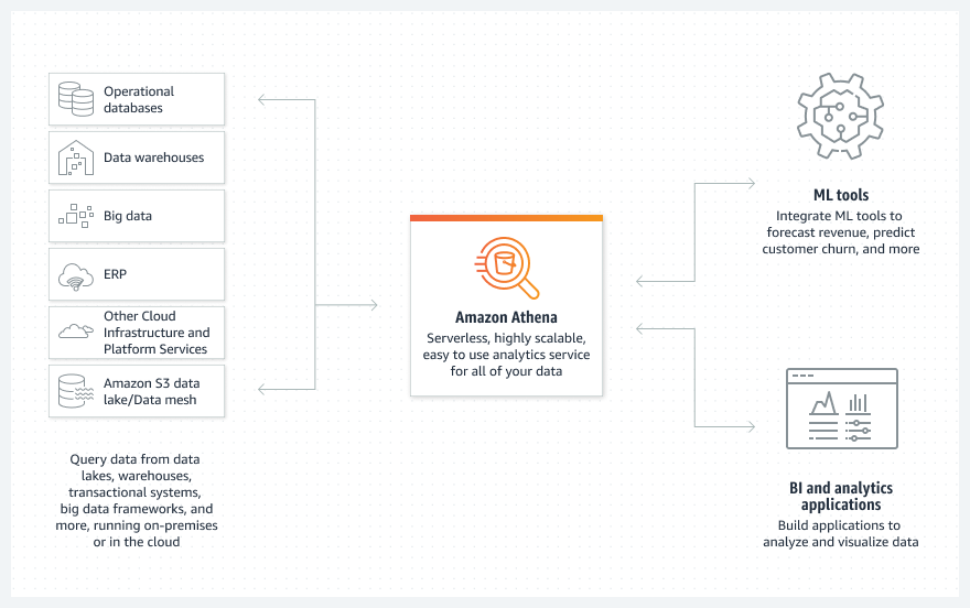
Amazon Athena now provides you more flexibility to use parameterized queries for any query you send to Athena, and we recommend you use them as the best practice for your Athena queries moving forward so you benefit from the security, reusability, and simplicity they offer. In a previous post, Improve reusability and security using Amazon Athena parameterized queries, we explained how parameterized queries with prepared statements provide reusability of queries, protection against SQL injection, and masking of query strings from AWS CloudTrail events. In this post, we explain how you can run Athena parameterized queries using the ExecutionParameters property in your StartQueryExecution requests. We provide a sample application you can reference for using parameterized queries, with and without prepared statements. Athena parameterized queries can be integrated into many data driven applications, and we walk you through a sample data as a service application to see how parameterized queries can plug in.
Customers tell us they are finding new ways to make effective use of their data assets by providing data as a service (DaaS). In this post, we share a sample architecture using parameterized queries applied in the form of a DaaS application. This is helpful for many types of organizations, whether you’re working with an enterprise making data available to other lines of business, a regulator making reports available to your industry, a company monetizing your data assets, an independent software vendor (ISV) enabling your applications’ tenants to query their data when they need it, or trying to share data at scale in other ways. In DaaS applications, you can provide predefined queries to run against your governed datasets with values your users input. You can expand your DaaS application to break away from monolithic data infrastructure by treating data as a product (DaaP) and providing a distribution of datasets, which have distinct domain-specific data pipelines. You can authorize these datasets to consumers in your DaaS application permissions. You can use Athena parameterized queries as a way to predefine your queries, which you can use to run queries across your datasets, and serve as a layer of protection for your DaaS applications. This post first describes how parameterized queries work, then applies parameterized queries in the form of a DaaS application.
Feature overview
In any query you send to Athena, you can use positional parameters declared by a question mark (?) in your query string, then declare values as execution parameters sequentially in your StartQueryExecution request. You can use execution parameters with your existing prepared statements and also with any SQL queries in Athena. You can still take advantage of the reusability and security benefits of parameterized queries, and using execution parameters also masks your query’s parameters when viewing recent queries in Athena. You can also change from building SQL query strings manually to using execution parameters; this allows you to run parameterized queries without needing to first create prepared statements. For more information on using execution parameters, refer to StartQueryExecution.
Previously, you could only run parameterized queries by first creating prepared statements in your Athena workgroup, then running parameterized queries while passing variables into an EXECUTE SQL statement with the USING clause. You are no longer required to create and maintain prepared statements across all of your Athena workgroups to take advantage of parameterization. This is helpful if you run the same queries across multiple workgroups or otherwise do not need the prepared statements feature.
You can continue to use Athena workgroups to isolate, implement individual cost constraints, and track query-related metrics for tenants within your multi-tenant application. For example, your DaaS application’s customers can run the same queries against your dataset with separate workgroups. For more information on Athena workgroups, refer to Using workgroups for running queries.
Changing your code to use parameterized queries
Changing your existing code to use parameterized queries is a small change which will have an immediate positive impact. Previously, you were required to build your query string value manually using environment variables as parameter placeholders. Manipulating the query string can be burdensome and has an inherent risk for injecting undesired values or SQL fragments (such as SQL operators), regardless of intent. You can now replace variables in your query string with a question mark (?), and declare your variable values sequentially with the ExecutionParameters option. By doing so, you take advantage of the security benefits of parameterized queries, and your queries are less complicated to author and maintain. The syntax change is shown in the following code, using the AWS Command Line Interface (AWS CLI) as an example.
Previously, running queries against Athena without execution parameters:
aws athena start-query-execution \
--query-string "SELECT * FROM table WHERE x = $ARG1 AND y = $ARG2 AND z = $ARG3" \
--query-execution-context "Database"="default" \
--work-group myWorkGroup
Now, running parameterized queries against Athena with execution parameters:
aws athena start-query-execution \
--query-string "SELECT * FROM table WHERE x = ? AND y = ? AND z = ?" \
--query-execution-context "Database"="default" \
--work-group myWorkGroup \
--execution-parameters $ARG1 $ARG2 $ARG3
The following is an example of a command that creates a prepared statement in your Athena workgroup. To learn more about creating prepared statements, refer to Querying with prepared statements.
aws athena start-query-execution \
--query-string "PREPARE my-prepared-statement FROM SELECT * FROM table WHERE x = ? AND y = ? AND z = ?" \
--query-execution-context "Database"="default" \
--work-group myWorkGroup
Previously, running parameterized queries against prepared statements without execution parameters:
aws athena start-query-execution \
--query-string "EXECUTE my-prepared-statement USING $ARG1, $ARG2, $ARG3“ \
--query-execution-context "Database"="default" \
--work-group myWorkGroup
Now, running parameterized queries against prepared statements with execution parameters:
aws athena start-query-execution \
--query-string "EXECUTE my-prepared-statement" \
--query-execution-context "Database"="default" \
--work-group myWorkGroup \
--execution-parameters $ARG1 $ARG2 $ARG3
Sample architecture
The purpose of this sample architecture is to apply the ExecutionParameters feature when running Athena queries, with and without prepared statements. This is not intended to be a DaaS solution for use with your production data.
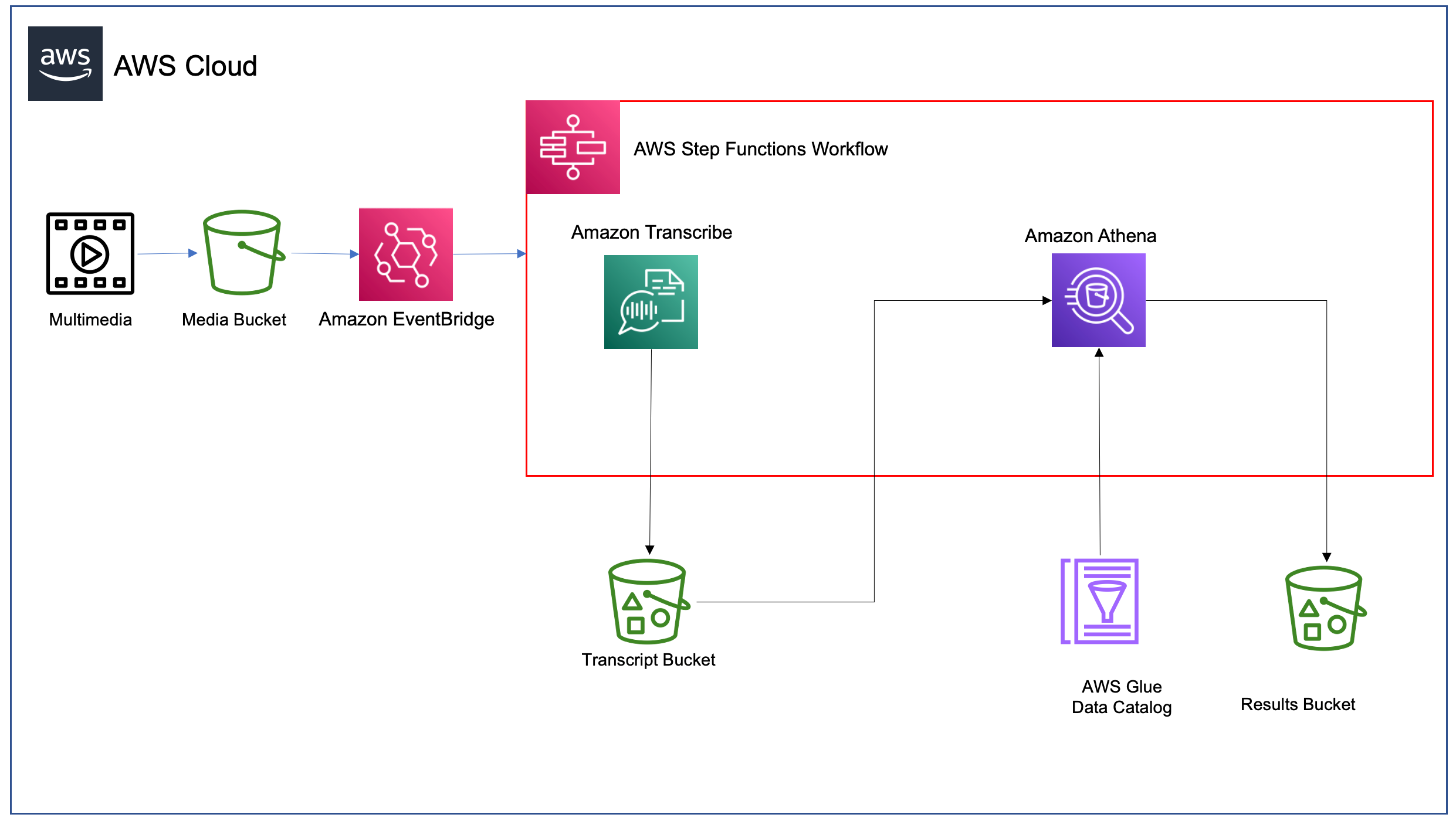
This sample architecture exhibits a DaaS application with a user interface (UI) that presents three Athena parameterized queries written against the public Amazon.com customer reviews dataset. The following figure depicts this workflow when a user submits a query to Athena. This example uses AWS Amplify to host a front-end application. The application calls an Amazon API Gateway HTTP API, which invokes AWS Lambda functions to authenticate requests, fetch the Athena prepared statements and named queries, and run the parameterized queries against Athena. The Lambda function uses the name of the Athena workgroup, statement name, statement type (prepared statement or not), and a list of query parameters input by the user. Athena queries data in an Amazon Simple Storage Service (Amazon S3), bucket which is cataloged in AWS Glue, and presents results to the user on the DaaS application UI.

End-users of the DaaS application UI can run only parameterized queries against Athena. The DaaS application UI demonstrates two ways to run parameterized queries with execution parameters: with and without prepared statements. In both cases, the Lambda function submits the query, waits for the query to complete, and provides the results that match the query parameters. The following figure depicts the DaaS application UI.

You may want your users to have the ability to list all Athena prepared statements within your Athena workgroup, select a statement, input arguments, and run the query; on the left side of the DaaS application UI, you use an EXECUTE statement to query the data lake with an Athena prepared statement. You may have several reporting queries maintained in your code base. In this case, your users select a statement, input arguments, and run the query. On the right side of the DaaS application UI, you use a SELECT statement to use Athena parameterized queries without prepared statements.
Prerequisites
This post uses the following AWS services to demonstrate a DaaS architecture pattern that uses Athena to query the Amazon.com customer reviews dataset:
- AWS Amplify
- Amazon API Gateway
- Amazon Athena
- AWS CloudFormation
- Amazon DynamoDB
- AWS Glue and the AWS Glue Data Catalog
- AWS Identity and Access Management (IAM)
- AWS Lambda
- Amazon S3
This post assumes you have the following:
- An AWS account. For instructions, refer to Creating an AWS account.
- A CloudTrail trail created. For instructions, refer to Creating a trail.
- An S3 bucket created. For instructions, refer to Creating a bucket.
- Node.js version 16+ installed on your device.
Deploy the CloudFormation stack
In this section, you deploy a CloudFormation template that creates the following resources:
- AWS Glue Data Catalog database
- AWS Glue Data Catalog table
- An Athena workgroup
- Three Athena prepared statements
- Three Athena named queries
- The API Gateway HTTP API
- The Lambda execution role for Athena queries
- The Lambda execution role for API Gateway HTTP API authorization
- Five Lambda functions:
- Update the AWS Glue Data Catalog
- Authorize API Gateway requests
- Submit Athena queries
- List Athena prepared statements
- List Athena named queries
Note that this CloudFormation template was tested in AWS Regions ap-southeast-2, ca-central-1, eu-west-2, us-east-1, us-east-2, and us-west-2. Note that deploying this into your AWS account will incur cost. Steps for cleaning up the resources are included later in this post.
To deploy the CloudFormation stack, follow these steps:
- Navigate to this post’s GitHub repository.
- Clone the repository or copy the CloudFormation template
athena-parameterized-queries.yaml. - On the AWS CloudFormation console, choose Create stack.
- Select Upload a template file and choose Choose file.
- Upload
athena-parameterized-queries.yaml, then choose Next. - On the Specify stack details page, enter the stack name
athena-parameterized-queries. - On the same page, there are two parameters:
- For S3QueryResultsBucketName, enter the S3 bucket name in your AWS account and in the same AWS Region as where you’re running your CloudFormation stack. (For this post, we use the bucket name value, like
my-bucket). - For APIPassphrase, enter a passphrase to authenticate API requests. You use this later.
- For S3QueryResultsBucketName, enter the S3 bucket name in your AWS account and in the same AWS Region as where you’re running your CloudFormation stack. (For this post, we use the bucket name value, like
- Choose Next.
- On the Configure stack options page, choose Next.
- On the Review page, select I acknowledge that AWS CloudFormation might create IAM resources with custom names, and choose Create stack.
The script takes less than two minutes to run and change to a CREATE_COMPLETE state. If you deploy the stack twice in the same AWS account and Region, some resources may already exist, and the process fails with a message indicating the resource already exists in another template.
- On the Outputs tab, copy the
APIEndpointvalue to use later.
For least-privilege authorization for deployment of the CloudFormation template, you can create an AWS CloudFormation service role with the following IAM policy actions. To do this, you must create an IAM policy and IAM role, and choose this role when configuring stack options. You need to replace the values for ${Partition}, ${AccountId}, and ${Region} with your own values; for more information on these values, refer to Pseudo parameters reference.
{
    "Version": "2012-10-17",
    "Statement": [
        {
            "Sid": "IAM",
            "Effect": "Allow",
            "Action": [
                "iam:GetRole",
                "iam:UntagRole",
                "iam:TagRole",
                "iam:CreateRole",
                "iam:DeleteRole",
                "iam:PassRole",
                "iam:GetRolePolicy",
                "iam:PutRolePolicy",
                "iam:AttachRolePolicy",
                "iam:TagPolicy",
                "iam:DeleteRolePolicy",
                "iam:DetachRolePolicy",
                "iam:UntagPolicy"
            ],
            "Resource": [
                "arn:${Partition}:iam::${AccountId}:role/LambdaAthenaExecutionRole-athena-parameterized-queries",
                "arn:${Partition}:iam::${AccountId}:role/service-role/LambdaAthenaExecutionRole-athena-parameterized-queries",
                "arn:${Partition}:iam::${AccountId}:role/service-role/LambdaAuthorizerExecutionRole-athena-parameterized-queries",
                "arn:${Partition}:iam::${AccountId}:role/LambdaAuthorizerExecutionRole-athena-parameterized-queries"
            ]
        },
        {
            "Sid": "LAMBDA",
            "Effect": "Allow",
            "Action": [
                "lambda:CreateFunction",
                "lambda:GetFunction",
                "lambda:InvokeFunction",
                "lambda:AddPermission",
                "lambda:DeleteFunction",
                "lambda:RemovePermission",
                "lambda:UpdateFunctionConfiguration"
            ],
            "Resource": [
                "arn:${Partition}:lambda:${Region}:${AccountId}:function:LambdaRepairFunction-athena-parameterized-queries",
                "arn:${Partition}:lambda:${Region}:${AccountId}:function:LambdaAthenaFunction-athena-parameterized-queries",
                "arn:${Partition}:lambda:${Region}:${AccountId}:function:LambdaAuthorizerFunction-athena-parameterized-queries",
                "arn:${Partition}:lambda:${Region}:${AccountId}:function:GetPrepStatements-athena-parameterized-queries",
                "arn:${Partition}:lambda:${Region}:${AccountId}:function:GetNamedQueries-athena-parameterized-queries"
            ]
        },
        {
            "Sid": "ATHENA",
            "Effect": "Allow",
            "Action": [
                "athena:GetWorkGroup",
                "athena:CreateWorkGroup",
                "athena:DeleteWorkGroup",
                "athena:DeleteNamedQuery",
                "athena:CreateNamedQuery",
                "athena:CreatePreparedStatement",
                "athena:DeletePreparedStatement",
                "athena:GetPreparedStatement"
            ],
            "Resource": [
                "arn:${Partition}:athena:${Region}:${AccountId}:workgroup/ParameterizedStatementsWG"
            ]
        },
        {
            "Sid": "GLUE",
            "Effect": "Allow",
            "Action": [
                "glue:CreateDatabase",
                "glue:DeleteDatabase",
                "glue:CreateTable",
                "glue:DeleteTable"
            ],
            "Resource": [
                "arn:${Partition}:glue:${Region}:${AccountId}:catalog",
                "arn:${Partition}:glue:${Region}:${AccountId}:database/athena_prepared_statements",
                "arn:${Partition}:glue:${Region}:${AccountId}:table/athena_prepared_statements/*",
                "arn:${Partition}:glue:${Region}:${AccountId}:userDefinedFunction/athena_prepared_statements/*"
            ]
        },
        {
            "Sid": "APIGATEWAY",
            "Effect": "Allow",
            "Action": [
                "apigateway:DELETE",
                "apigateway:PUT",
                "apigateway:PATCH",
                "apigateway:POST",
                "apigateway:TagResource",
                "apigateway:UntagResource"
            ],
            "Resource": [
                "arn:${Partition}:apigateway:${Region}::/apis/*/integrations*",
                "arn:${Partition}:apigateway:${Region}::/apis/*/stages*",
                "arn:${Partition}:apigateway:${Region}::/apis/*/authorizers*",
                "arn:${Partition}:apigateway:${Region}::/apis/*/routes*",
                "arn:${Partition}:apigateway:${Region}::/tags/arn%3Aaws%3Aapigateway%3A${Region}%3A%3A%2Fv2%2Fapis%2F*"
            ]
        },
        {
            "Sid": "APIGATEWAYMANAGEAPI",
            "Effect": "Allow",
            "Action": [
                "apigateway:DELETE",
                "apigateway:PUT",
                "apigateway:PATCH",
                "apigateway:POST",
                "apigateway:GET"
            ],
            "Resource": [
                "arn:${Partition}:apigateway:${Region}::/apis"
            ],
            "Condition": {
                "StringEquals": {
                    "apigateway:Request/ApiName": "AthenaAPI-athena-parameterized-queries"
                }
            }
        },
        {
            "Sid": "APIGATEWAYMANAGEAPI2",
            "Effect": "Allow",
            "Action": [
                "apigateway:DELETE",
                "apigateway:PUT",
                "apigateway:PATCH",
                "apigateway:POST",
                "apigateway:GET"
            ],
            "Resource": [
                "arn:${Partition}:apigateway:${Region}::/apis/*"
            ],
            "Condition": {
                "StringEquals": {
                    "apigateway:Resource/ApiName": "AthenaAPI-athena-parameterized-queries"
                }
            }
        },
        {
            "Sid": "APIGATEWAYGET",
            "Effect": "Allow",
            "Action": [
                "apigateway:GET"
            ],
            "Resource": [
                "arn:${Partition}:apigateway:${Region}::/apis/*"
            ]
        },
        {
            "Sid": "LAMBDALAYER",
            "Effect": "Allow",
            "Action": [
                "lambda:GetLayerVersion"
            ],
            "Resource": [
                "arn:${Partition}:lambda:*:280475519630:layer:boto3-1_24*"
            ]
        }
    ]
}
After you create the CloudFormation stack, you use the AWS management console to deploy an Amplify application and view the Lambda functions. The following is the scoped-down IAM policy that you can attach to an IAM user or role to perform these operations:
{
    "Version": "2012-10-17",
    "Statement": [
        {
            "Sid": "AmplifyCreateApp",
            "Effect": "Allow",
            "Action": [
                "amplify:CreateBranch",
                "amplify:StartDeployment",
                "amplify:CreateDeployment",
                "amplify:CreateApp",
                "amplify:StartJob"
            ],
            "Resource": "arn:${Partition}:amplify:${Region}:${AccountId}:apps/*"
        },
        {
            "Sid": "AmplifyList",
            "Effect": "Allow",
            "Action": "amplify:List*",
            "Resource": "arn:${Partition}:amplify:${Region}:${AccountId}:apps/*"
        },
        {
            "Sid": "AmplifyGet",
            "Effect": "Allow",
            "Action": "amplify:GetJob",
            "Resource": "arn:${Partition}:amplify:${Region}:${AccountId}:apps/*"
        },
        {
            "Sid": "LambdaList",
            "Effect": "Allow",
            "Action": [
                "lambda:GetAccountSettings",
                "lambda:ListFunctions"
            ],
            "Resource": "*"
        },
        {
            "Sid": "LambdaFunction",
            "Effect": "Allow",
            "Action": [
                "lambda:GetFunction"
            ],
            "Resource": "arn:${Partition}:lambda:${Region}:${AccountId}:function:LambdaAthenaFunction-athena-parameterized-queries"
        }
    ]
}
Note that you need the following IAM policy when deploying your Amplify application to set a global password, and when cleaning up your resources to delete the Amplify application. Remember to replace ${AppARN} with the ARN of the Amplify application. You can find the ARN after creating the Amplify app on the General tab in the App Settings section of the Amplify console.
{
   "Version": "2012-10-17",
   "Statement": [
       {
           "Sid": "UpdateAndDeleteAmplifyApp",
           "Effect": "Allow",
            "Action": [
                "amplify:DeleteApp",
                "amplify:UpdateApp"
            ],
           "Resource": "${AppARN}"
       }
   ]
}
Deploy the Amplify application
In this section, you deploy your Amplify application.
- In the cloned repository, open
web-application/.envin a text editor. - Set
AWS_API_ENDPOINTas theAPIEndpointvalue from the CloudFormation stack Outputs For example:AWS_API_ENDPOINT="https://123456abcd.execute-api.your-region.amazonaws.com". - Set
API_AUTH_CODEas the value you input as the CloudFormation stack’sAPIPassphraseparameter argument. For example:API_AUTH_CODE="YOUR_PASSPHRASE". - Navigate to the
web-application/directory and runnpm install. - Run
npm run buildto compile distribution assets. - On the Amplify console, choose All apps.
- Choose New app.
- Select Host web app, select Deploy without Git provider, then choose Continue.
- For App name, enter
Athena Parameterized Queries App. - For Environment name¸ you don’t need to enter a value.
- Select Drag and Drop.
- Locate the
dist/directory insideweb-application/, drag it into the window and drop it. Ensure you drag the entire directory, not the files within it.
- Choose Save and deploy to deploy the web application on Amplify.

This step takes less than a minute to complete.
- Under App settings, choose Access control, then choose Manage access.
- Select Apply a global password, then enter values for Username and Password.
You use these credentials to access your Amplify application.
Access your Amplify application and run queries
In this section, you use the Amplify application to run Athena parameterized queries against the Amazon.com customer reviews dataset. The left side of the application shows how you can run parameterized queries using Athena prepared statements. The right side of the application shows how you can run parameterized queries without prepared statements, such as if the queries are written in your code. The sample in this post uses named queries within the Athena workgroup. For more information about named queries, refer to NamedQuery.
- Open the Amplify web application link located under Domain. For example:
https://dev123.abcd12345xyz.amplifyapp.com/. - In the Sign in prompt, enter the user name and password you provided as the Amplify application global password.
- For Workgroup Name, choose the
ParameterizedStatementsWGworkgroup. - Choose a statement example on the Prepared Statement or SQL Statement drop-down menu.
Selecting a statement displays a description about the query, including examples of parameters you can try with this statement, and the original SQL query string. SQL parameters of type string must be surrounded by single quotes, for example: 'your_string_value'.
- Enter your query parameters.
The following figure shows an example of the parameters to input for the product_helpful_reviews prepared statement.

- Choose Run Query to send the query request to the API endpoint.
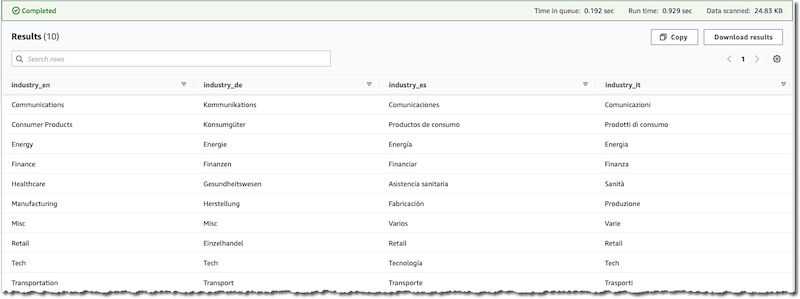
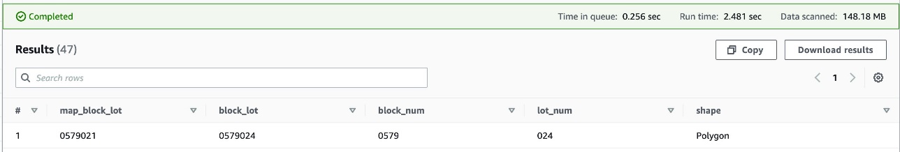
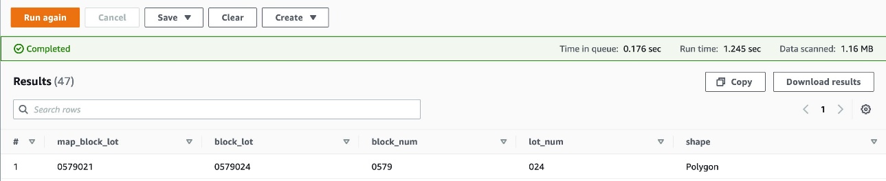
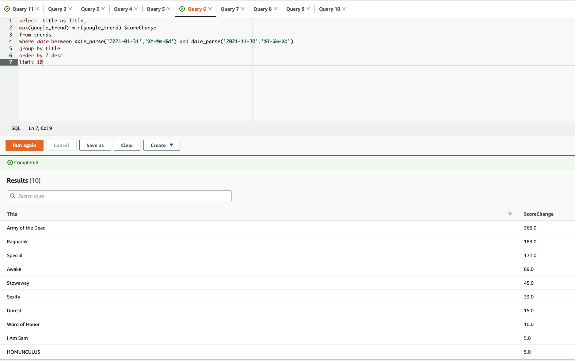
After the query runs, the sample application presents the results in a table format, as depicted in the following screenshot. This is one of many ways to present results, and your application can display results in the format which makes the most sense for your users. The complete query workflow is depicted in the previous architecture diagram.

Using execution parameters with the AWS SDK for Python (Boto3)
In this section, you inspect the Lambda function code for using the StartQueryExecution API with and without prepared statements.
- On the Lambda console, choose Functions.
- Navigate to the
LambdaAthenaFunction-athena-parameterized-queriesfunction. - Choose the Code Source window.
Examples of passing parameters to the Athena StartQueryExecution API using the AWS SDK for Python (Boto3) begin on lines 39 and 49. Note the ExecutionParameters option on lines 45 and 55.
The following code uses execution parameters with Athena prepared statements:
response = athena.start_query_execution(
    QueryString=f'EXECUTE {statement}', # Example: "EXECUTE prepared_statement_name"
    WorkGroup=workgroup,
    QueryExecutionContext={
        'Database': 'athena_prepared_statements'
    },
    ExecutionParameters=input_parameters
)
The following code uses execution parameters without Athena prepared statements:
response = athena.start_query_execution(
    QueryString=statement, # Example: "SELECT * FROM TABLE WHERE parameter_name = ?"
    WorkGroup=workgroup,
    QueryExecutionContext={
        'Database': 'athena_prepared_statements'
    },
    ExecutionParameters=input_parameters
)
Clean up
In this post, you created several components, which generate cost. To avoid incurring future charges, remove the resources with the following steps:
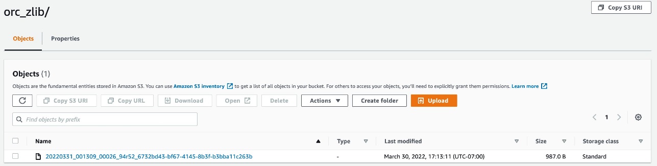
- Delete the S3 bucket’s results prefix created after you ran a query on your workgroup.
With the default template, the prefix is named <S3QueryResultsBucketName>/athena-results. Use caution in this step. Unless you are using versioning on your S3 bucket, deleting S3 objects can’t be undone.
- On the Amplify console, select the app to delete and on the Actions menu, choose Delete app, then confirm.
- On the AWS CloudFormation console, select the stack to delete, choose Delete, and confirm.
Conclusion
In this post, we showed how you can build a DaaS application using Athena parameterized queries. The StartQueryExecution API in Athena now supports execution parameters, which allows you to run any Athena query as a parameterized query. You can decouple your execution parameters from your query strings, and use parameterized queries without being limited to the Athena workgroups where you have created prepared statements. You can take advantage of the security benefits Athena offers with parameterized queries, and developers no longer need to build query strings manually. In this post, you learned how to use execution parameters, and you deployed a DaaS reference architecture to see how parameterized queries can be applied.
You can get started with Athena parameterized queries by using the Athena console, the AWS CLI, or the AWS SDK. To learn more about Athena, refer to the Amazon Athena User Guide.
Thanks for reading this post! If you have questions about Athena prepared statements and parameterized queries, don’t hesitate to leave a comment.
About the Authors
 Blayze Stefaniak is a Senior Solutions Architect for the Technical Strategist Program supporting Executive Customer Programs in AWS Marketing. He has experience working across industries including healthcare, automotive, and public sector. He is passionate about breaking down complex situations into something practical and actionable. In his spare time, you can find Blayze listening to Star Wars audiobooks, trying to make his dogs laugh, and probably talking on mute.
 Daniel Tatarkin is a Solutions Architect at Amazon Web Services (AWS) supporting Federal Financial organizations. He is passionate about big data analytics and serverless technologies. Outside of work, he enjoys learning about personal finance, coffee, and trying out new programming languages for fun.
 Matt Boyd is a Senior Solutions Architect at AWS working with federal financial organizations. He is passionate about effective cloud management and governance, as well as data governance strategies. When he’s not working, he enjoys running, weight lifting, and teaching his elementary-age son ethical hacking skills.


 Varad Ram is Senior Solutions Architect in Amazon Web Services. He likes to help customers adopt to cloud technologies and is particularly interested in artificial intelligence. He believes deep learning will power future technology growth. In his spare time, he like to be outdoor with his daughter and son.


 Francesco Marelli is a principal solutions architect at Amazon Web Services. He is specialized in the design and implementation of analytics, data management, and big data systems. Francesco also has a strong experience in systems integration and design and implementation of applications. He is passionate about music, collecting vinyl records, and playing bass.


 Suresh Akena is a Principal WW GTM Leader for Amazon Athena. He works with the startups, enterprise and strategic customers to provide leadership on large scale data strategies including migration to AWS platform, big data and analytics and ML initiatives and help them to optimize and improve time to market for data driven applications when using AWS.
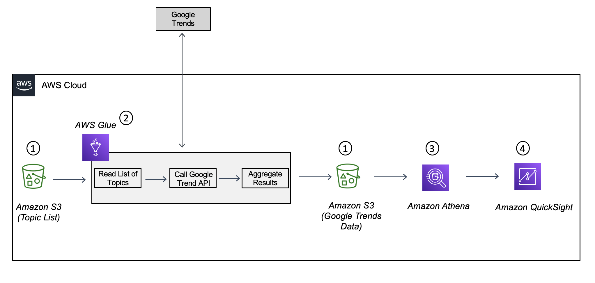


 Anand Shah is a Big Data Prototyping Solution Architect at AWS. He works with AWS customers and their engineering teams to build prototypes using AWS analytics services and purpose-built databases. Anand helps customers solve the most challenging problems using the art of the possible technology. He enjoys beaches in his leisure time.