Tag Archives: Analytics

Accelerate orchestration of an ELT process using AWS Step Functions and Amazon Redshift Data API

2023-01-10 Poulomi Dasgupta

Post Syndicated from Poulomi Dasgupta original https://aws.amazon.com/blogs/big-data/accelerate-orchestration-of-an-elt-process-using-aws-step-functions-and-amazon-redshift-data-api/

Extract, Load, and Transform (ELT) is a modern design strategy where raw data is first loaded into the data warehouse and then transformed with familiar Structured Query Language (SQL) semantics leveraging the power of massively parallel processing (MPP) architecture of the data warehouse. When you use an ELT pattern, you can also use your existing SQL workload while migrating from your on-premises data warehouse to Amazon Redshift. This eliminates the need to rewrite relational and complex SQL workloads into a new framework. With Amazon Redshift, you can load, transform, and enrich your data efficiently using familiar SQL with advanced and robust SQL support, simplicity, and seamless integration with your existing SQL tools. When you adopt an ELT pattern, a fully automated and highly scalable workflow orchestration mechanism will help to minimize the operational effort that you must invest in managing the pipelines. It also ensures the timely and accurate refresh of your data warehouse.

AWS Step Functions is a low-code, serverless, visual workflow service where you can orchestrate complex business workflows with an event-driven framework and easily develop repeatable and dependent processes. It can ensure that the long-running, multiple ELT jobs run in a specified order and complete successfully instead of manually orchestrating those jobs or maintaining a separate application.

Amazon DynamoDB is a fast, flexible NoSQL database service for single-digit millisecond performance at any scale.

This post explains how to use AWS Step Functions, Amazon DynamoDB, and Amazon Redshift Data API to orchestrate the different steps in your ELT workflow and process data within the Amazon Redshift data warehouse.

Solution overview

In this solution, we will orchestrate an ELT process using AWS Step Functions. As part of the ELT process, we will refresh the dimension and fact tables at regular intervals from staging tables, which ingest data from the source. We will maintain the current state of the ELT process (e.g., Running or Ready) in an audit table that will be maintained at Amazon DynamoDB. AWS Step Functions allows you to directly call the Data API from a state machine, reducing the complexity of running the ELT pipeline. For loading the dimensions and fact tables, we will be using Amazon Redshift Data API from AWS Lambda. We will use Amazon EventBridge for scheduling the state machine to run at a desired interval based on the customer’s SLA.

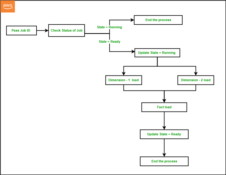
For a given ELT process, we will set up a JobID in a DynamoDB audit table and set the JobState as “Ready” before the state machine runs for the first time. The state machine performs the following steps:

The first process in the Step Functions workflow is to pass the JobID as input to the process that is configured as JobID 101 in Step Functions and DynamoDB by default via the CloudFormation template.
The next step is to fetch the current JobState for the given JobID by running a query against the DynamoDB audit table using Lambda Data API.
If JobState is “Running,” then it indicates that the previous iteration is not completed yet, and the process should end.
If the JobState is “Ready,” then it indicates that the previous iteration was completed successfully and the process is ready to start. So, the next step will be to update the DynamoDB audit table to change the JobState to “Running” and JobStart to the current time for the given JobID using DynamoDB Data API within a Lambda function.
The next step will be to start the dimension table load from the staging table data within Amazon Redshift using Lambda Data API. In order to achieve that, we can either call a stored procedure using the Amazon Redshift Data API, or we can also run series of SQL statements synchronously using Amazon Redshift Data API within a Lambda function.
In a typical data warehouse, multiple dimension tables are loaded in parallel at the same time before the fact table gets loaded. Using Parallel flow in Step Functions, we will load two dimension tables at the same time using Amazon Redshift Data API within a Lambda function.
Once the load is completed for both the dimension tables, we will load the fact table as the next step using Amazon Redshift Data API within a Lambda function.
As the load completes successfully, the last step would be to update the DynamoDB audit table to change the JobState to “Ready” and JobEnd to the current time for the given JobID, using DynamoDB Data API within a Lambda function.

Components and dependencies

The following architecture diagram highlights the end-to-end solution using AWS services:

Before diving deeper into the code, let’s look at the components first:

AWS Step Functions – You can orchestrate a workflow by creating a State Machine to manage failures, retries, parallelization, and service integrations.
Amazon EventBridge – You can run your state machine on a daily schedule by creating a Rule in Amazon EventBridge.
AWS Lambda – You can trigger a Lambda function to run Data API either from Amazon Redshift or DynamoDB.
Amazon DynamoDB – Amazon DynamoDB is a fully managed, serverless, key-value NoSQL database designed to run high-performance applications at any scale. DynamoDB is extremely efficient in running updates, which improves the performance of metadata management for customers with strict SLAs.
Amazon Redshift – Amazon Redshift is a fully managed, scalable cloud data warehouse that accelerates your time to insights with fast, easy, and secure analytics at scale.
Amazon Redshift Data API – You can access your Amazon Redshift database using the built-in Amazon Redshift Data API. Using this API, you can access Amazon Redshift data with web services–based applications, including AWS Lambda.
DynamoDB API – You can access your Amazon DynamoDB tables from a Lambda function by importing boto3.

Prerequisites

To complete this walkthrough, you must have the following prerequisites:

An AWS account.
An Amazon Redshift cluster.
An Amazon Redshift customizable IAM service role with the following policies:
- AmazonS3ReadOnlyAccess
- AmazonRedshiftFullAccess
Above IAM role associated to the Amazon Redshift cluster.

Deploy the CloudFormation template

To set up the ETL orchestration demo, the steps are as follows:

Sign in to the AWS Management Console.
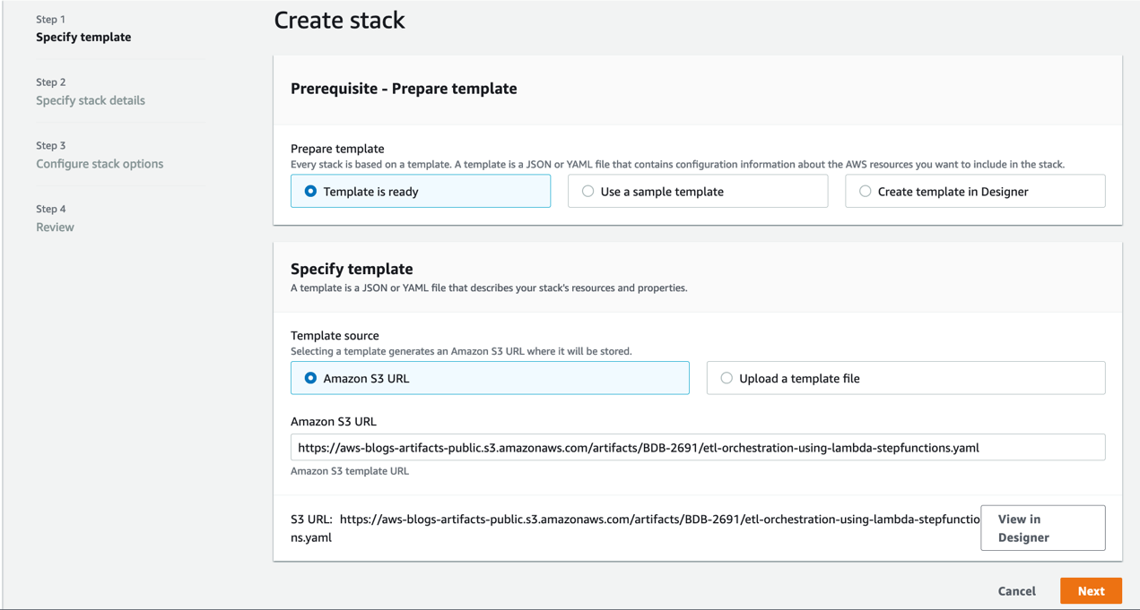
Click on Launch Stack.
Click Next.
Enter a suitable name in Stack name.
Provide the information for the Parameters as detailed in the following table.

CloudFormation template parameter	Allowed values	Description
`RedshiftClusterIdentifier`	Amazon Redshift cluster identifier	Enter the Amazon Redshift cluster identifier
`DatabaseUserName`	Database user name in Amazon Redshift cluster	Amazon Redshift database user name which has access to run SQL Script
`DatabaseName`	Amazon Redshift database name	Name of the Amazon Redshift primary database where SQL script would be run
`RedshiftIAMRoleARN`	Valid IAM role ARN attached to Amazon Redshift cluster	AWS IAM role ARN associated with the Amazon Redshift cluster

Click Next and a new page appears. Accept the default values in the page and click Next. On the last page check the box to acknowledge resources might be created and click on Create stack.
Monitor the progress of the stack creation and wait until it is complete.
The stack creation should complete approximately within 5 minutes.
Navigate to Amazon Redshift console.
Launch Amazon Redshift query editor v2 and connect to your cluster.
Browse to the database name provided in the parameters while creating the cloudformation template e.g., dev, public schema and expand Tables. You should see the tables as shown below.
Validate the sample data by running the following SQL query and confirm the row count match above the screenshot.

select 'customer',count(*) from public.customer
union all
select 'fact_yearly_sale',count(*) from public.fact_yearly_sale
union all
select 'lineitem',count(*) from public.lineitem
union all
select 'nation',count(*) from public.nation
union all
select 'orders',count(*) from public.orders
union all
select 'supplier',count(*) from public.supplier

Run the ELT orchestration

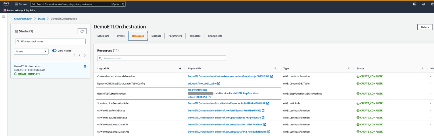
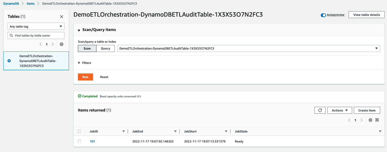
After you deploy the CloudFormation template, navigate to the stack detail page. On the Resources tab, choose the link for DynamoDBETLAuditTable to be redirected to the DynamoDB console.
Navigate to Tables and click on table name beginning with <stackname>-DynamoDBETLAuditTable. In this demo, the stack name is DemoETLOrchestration, so the table name will begin with DemoETLOrchestration-DynamoDBETLAuditTable.
It will expand the table. Click on Explore table items.
Here you can see the current status of the job, which will be in Ready status.
Navigate again to stack detail page on the CloudFormation console. On the Resources tab, choose the link for RedshiftETLStepFunction to be redirected to the Step Functions console.
Click Start Execution. When it successfully completes, all steps will be marked as green.
While the job is running, navigate back to DemoETLOrchestration-DynamoDBETLAuditTable in the DynamoDB console screen. You will see JobState as Running with JobStart time.

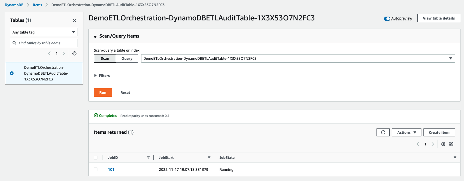
After Step Functions completes, JobState will be changed to Ready with JobStart and JobEnd time.

Handling failure

In the real world sometimes, the ELT process can fail due to unexpected data anomalies or object related issues. In that case, the step function execution will also fail with the failed step marked in red as shown in the screenshot below:

Once you identify and fix the issue, please follow the below steps to restart the step function:

Navigate to the DynamoDB table beginning with DemoETLOrchestration-DynamoDBETLAuditTable. Click on Explore table items and select the row with the specific JobID for the failed job.
Go to Action and select Edit item to modify the JobState to Ready as shown below:
Follow steps 5 and 6 under the “Run the ELT orchestration” section to restart execution of the step function.

Validate the ELT orchestration

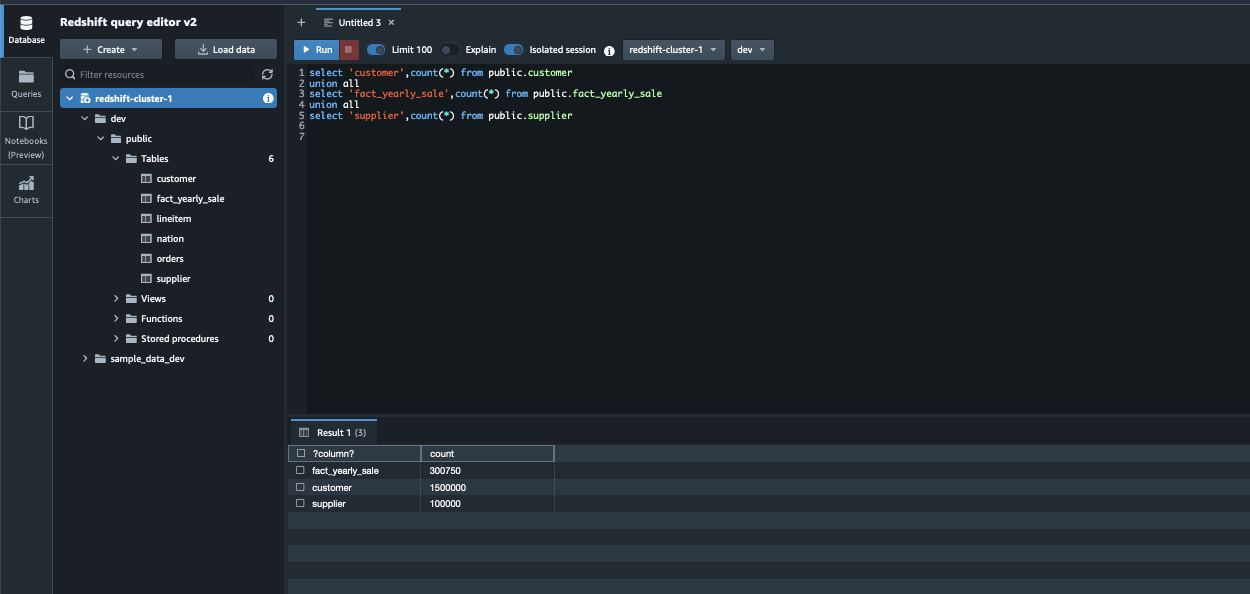
The step function loads the dimension tables public.supplier and public.customer and the fact table public.fact_yearly_sale. To validate the orchestration, the process steps are as follows:

Navigate to the Amazon Redshift console.
Launch Amazon Redshift query editor v2 and connect to your cluster.
Browse to the database name provided in the parameters while creating the cloud formation template e.g., dev, public schema.
Validate the data loaded by Step Functions by running the following SQL query and confirm the row count to match as follows:

select 'customer',count(*) from public.customer
union all
select 'fact_yearly_sale',count(*) from public.fact_yearly_sale
union all
select 'supplier',count(*) from public.supplier

Schedule the ELT orchestration

The steps are as follows to schedule the Step Functions:

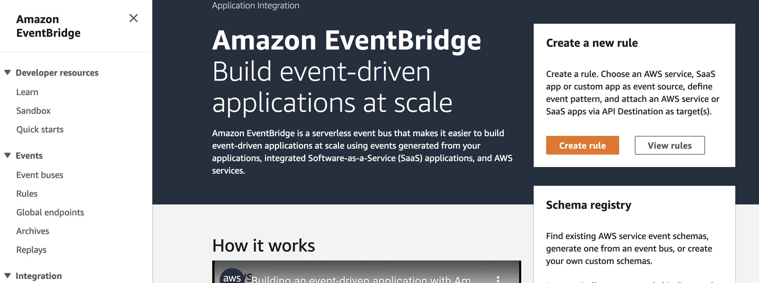
Navigate to the Amazon EventBridge console and choose Create rule.

Under Name, enter a meaningful name, for example, Trigger-Redshift-ELTStepFunction.
Under Event bus, choose default.
Under Rule Type, select Schedule.
Click on Next.
Under Schedule pattern, select A schedule that runs at a regular rate, such as every 10 minutes.
Under Rate expression, enter Value as 5 and choose Unit as Minutes.
Click on Next.
Under Target types, choose AWS service.
Under Select a Target, choose Step Functions state machine.
Under State machine, choose the step function created by the CloudFormation template.
Under Execution role, select Create a new role for this specific resource.
Click on Next.
Review the rule parameters and click on Create Rule.

After the rule has been created, it will automatically trigger the step function every 5 minutes to perform ELT processing in Amazon Redshift.

Clean up

Please note that deploying a CloudFormation template incurs cost. To avoid incurring future charges, delete the resources you created as part of the CloudFormation stack by navigating to the AWS CloudFormation console, selecting the stack, and choosing Delete.

Conclusion

In this post, we described how to easily implement a modern, serverless, highly scalable, and cost-effective ELT workflow orchestration process in Amazon Redshift using AWS Step Functions, Amazon DynamoDB and Amazon Redshift Data API. As an alternate solution, you can also use Amazon Redshift for metadata management instead of using Amazon DynamoDB. As part of this demo, we show how a single job entry in DynamoDB gets updated for each run, but you can also modify the solution to maintain a separate audit table with the history of each run for each job, which would help with debugging or historical tracking purposes. Step Functions manage failures, retries, parallelization, service integrations, and observability so your developers can focus on higher-value business logic. Step Functions can integrate with Amazon SNS to send notifications in case of failure or success of the workflow. Please follow this AWS Step Functions documentation to implement the notification mechanism.

About the Authors

Poulomi Dasgupta is a Senior Analytics Solutions Architect with AWS. She is passionate about helping customers build cloud-based analytics solutions to solve their business problems. Outside of work, she likes travelling and spending time with her family.

Raks Khare is an Analytics Specialist Solutions Architect at AWS based out of Pennsylvania. He helps customers architect data analytics solutions at scale on the AWS platform.

Tahir Aziz is an Analytics Solution Architect at AWS. He has worked with building data warehouses and big data solutions for over 13 years. He loves to help customers design end-to-end analytics solutions on AWS. Outside of work, he enjoys traveling
and cooking.

Add your own libraries and application dependencies to Spark and Hive on Amazon EMR Serverless with custom images

2023-01-10 Veena Vasudevan

Post Syndicated from Veena Vasudevan original https://aws.amazon.com/blogs/big-data/add-your-own-libraries-and-application-dependencies-to-spark-and-hive-on-amazon-emr-serverless-with-custom-images/

Amazon EMR Serverless allows you to run open-source big data frameworks such as Apache Spark and Apache Hive without managing clusters and servers. Many customers who run Spark and Hive applications want to add their own libraries and dependencies to the application runtime. For example, you may want to add popular open-source extensions to Spark, or add a customized encryption-decryption module that is used by your application.

We are excited to announce a new capability that allows you to customize the runtime image used in EMR Serverless by adding custom libraries that your applications need to use. This feature enables you to do the following:

Maintain a set of version-controlled libraries that are reused and available for use in all your EMR Serverless jobs as part of the EMR Serverless runtime
Add popular extensions to open-source Spark and Hive frameworks such as pandas, NumPy, matplotlib, and more that you want your EMR serverless application to use
Use established CI/CD processes to build, test, and deploy your customized extension libraries to the EMR Serverless runtime
Apply established security processes, such as image scanning, to meet the compliance and governance requirements within your organization
Use a different version of a runtime component (for example the JDK runtime or the Python SDK runtime) than the version that is available by default with EMR Serverless

In this post, we demonstrate how to use this new feature.

Solution Overview

To use this capability, customize the EMR Serverless base image using Amazon Elastic Container Registry (Amazon ECR), which is a fully managed container registry that makes it easy for your developers to share and deploy container images. Amazon ECR eliminates the need to operate your own container repositories or worry about scaling the underlying infrastructure. After the custom image is pushed to the container registry, specify the custom image while creating your EMR Serverless applications.

The following diagram illustrates the steps involved in using custom images for your EMR Serverless applications.

In the following sections, we demonstrate using custom images with Amazon EMR Serverless to address three common use cases:

Add popular open-source Python libraries into the EMR Serverless runtime image
Use a different or newer version of the Java runtime for the EMR Serverless application
Install a Prometheus agent and customize the Spark runtime to push Spark JMX metrics to Amazon Managed Service for Prometheus, and visualize the metrics in a Grafana dashboard

General prerequisites

The following are the prerequisites to use custom images with EMR Serverless. Complete the following steps before proceeding with the subsequent steps:

Create an AWS Identity and Access Management (IAM) role with IAM permissions for Amazon EMR Serverless applications, Amazon ECR permissions, and Amazon S3 permissions for the Amazon Simple Storage Service (Amazon S3) bucket aws-bigdata-blog and any S3 bucket in your account where you will store the application artifacts.
Install or upgrade to the latest AWS Command Line Interface (AWS CLI) version and install the Docker service in an Amazon Linux 2 based Amazon Elastic Compute Cloud (Amazon EC2) instance. Attach the IAM role from the previous step for this EC2 instance.
Select a base EMR Serverless image from the following public Amazon ECR repository. Run the following commands on the EC2 instance with Docker installed to verify that you are able to pull the base image from the public repository:
```
# If docker is not started already, start the process
$ sudo service docker start 

# Check if you are able to pull the latest EMR 6.9.0 runtime base image 
$ sudo docker pull public.ecr.aws/emr-serverless/spark/emr-6.9.0:latest
```

Log in to Amazon ECR with the following commands and create a repository called emr-serverless-ci-examples, providing your AWS account ID and Region:

$ sudo aws ecr get-login-password --region <region> | sudo docker login --username AWS --password-stdin <your AWS account ID>.dkr.ecr.<region>.amazonaws.com

$ aws ecr create-repository --repository-name emr-serverless-ci-examples --region <region>

Provide IAM permissions to the EMR Serverless service principal for the Amazon ECR repository:

On the Amazon ECR console, choose Permissions under Repositories in the navigation pane.
Choose Edit policy JSON.

Enter the following JSON and save:

{
  "Version": "2012-10-17",
  "Statement": [
    {
      "Sid": "Emr Serverless Custom Image Support",
      "Effect": "Allow",
      "Principal": {
        "Service": "emr-serverless.amazonaws.com"
      },
      "Action": [
        "ecr:BatchGetImage",
        "ecr:DescribeImages",
        "ecr:GetDownloadUrlForLayer"
      ]
    }
  ]
}

Make sure that the policy is updated on the Amazon ECR console.

For production workloads, we recommend adding a condition in the Amazon ECR policy to ensure only allowed EMR Serverless applications can get, describe, and download images from this repository. For more information, refer to Allow EMR Serverless to access the custom image repository.

In the next steps, we create and use custom images in our EMR Serverless applications for the three different use cases.

Use case 1: Run data science applications

One of the common applications of Spark on Amazon EMR is the ability to run data science and machine learning (ML) applications at scale. For large datasets, Spark includes SparkML, which offers common ML algorithms that can be used to train models in a distributed fashion. However, you often need to run many iterations of simple classifiers to fit for hyperparameter tuning, ensembles, and multi-class solutions over small-to-medium-sized data (100,000 to 1 million records). Spark is a great engine to run multiple iterations of such classifiers in parallel. In this example, we demonstrate this use case, where we use Spark to run multiple iterations of an XGBoost model to select the best parameters. The ability to include Python dependencies in the EMR Serverless image should make it easy to make the various dependencies (xgboost, sk-dist, pandas, numpy, and so on) available for the application.

Prerequisites

The EMR Serverless job runtime IAM role should be given permissions to your S3 bucket where you will be storing your PySpark file and application logs:

{
    "Version": "2012-10-17",
    "Statement": [
        {
            "Sid": "AccessToS3Buckets",
            "Effect": "Allow",
            "Action": [
                "s3:PutObject",
                "s3:GetObject",
                "s3:ListBucket"
            ],
            "Resource": [
                "arn:aws:s3:::<YOUR-BUCKET>",
                "arn:aws:s3:::<YOUR-BUCKET>/*"
            ]
        }
    ]
}

Create an image to install ML dependencies

We create a custom image from the base EMR Serverless image to install dependencies required by the SparkML application. Create the following Dockerfile in your EC2 instance that runs the docker process inside a new directory named datascience:

FROM public.ecr.aws/emr-serverless/spark/emr-6.9.0:latest

USER root

# python packages
RUN pip3 install boto3 pandas numpy
RUN pip3 install -U scikit-learn==0.23.2 scipy 
RUN pip3 install sk-dist
RUN pip3 install xgboost
RUN sed -i 's|import Parallel, delayed|import Parallel, delayed, logger|g' /usr/local/lib/python3.7/site-packages/skdist/distribute/search.py

# EMRS will run the image as hadoop
USER hadoop:hadoop

Build and push the image to the Amazon ECR repository emr-serverless-ci-examples, providing your AWS account ID and Region:

# Build the image locally. This command will take a minute or so to complete
sudo docker build -t local/emr-serverless-ci-ml /home/ec2-user/datascience/ --no-cache --pull
# Create tag for the local image
sudo docker tag local/emr-serverless-ci-ml:latest <your AWS account ID>.dkr.ecr.<region>.amazonaws.com/emr-serverless-ci-examples:emr-serverless-ci-ml
# Push the image to Amazon ECR. This command will take a few seconds to complete
sudo docker push <your AWS account ID>.dkr.ecr.<region>.amazonaws.com/emr-serverless-ci-examples:emr-serverless-ci-ml

Submit your Spark application

Create an EMR Serverless application with the custom image created in the previous step:

aws --region <region>  emr-serverless create-application \
    --release-label emr-6.9.0 \
    --type "SPARK" \
    --name data-science-with-ci \
    --image-configuration '{ "imageUri": "<your AWS account ID>.dkr.ecr.<region>.amazonaws.com/emr-serverless-ci-examples:emr-serverless-ci-ml" }'

Make a note of the value of applicationId returned by the command.

After the application is created, we’re ready to submit our job. Copy the application file to your S3 bucket:

aws s3 cp s3://aws-bigdata-blog/artifacts/BDB-2771/code/emrserverless-xgboost-spark-example.py s3://<YOUR BUCKET>/<PREFIX>/emrserverless-xgboost-spark-example.py

Submit the Spark data science job. In the following command, provide the name of the S3 bucket and prefix where you stored your application file. Additionally, provide the applicationId value obtained from the create-application command and your EMR Serverless job runtime IAM role ARN.

aws emr-serverless start-job-run \
        --region <region> \
        --application-id <applicationId> \
        --execution-role-arn <jobRuntimeRole> \
        --job-driver '{
            "sparkSubmit": {
                "entryPoint": "s3://<YOUR BUCKET>/<PREFIX>/emrserverless-xgboost-spark-example.py"
            }
        }' \
        --configuration-overrides '{
              "monitoringConfiguration": {
                "s3MonitoringConfiguration": {
                  "logUri": "s3://<YOUR BUCKET>/emrserverless/logs"
                }
              }
            }'

After the Spark job succeeds, you can view the best model estimates from our application by viewing the Spark driver’s stdout logs. Navigate to Spark History Server, Executors, Driver, Logs, stdout.

Use case 2: Use a custom Java runtime environment

Another use case for custom images is the ability to use a custom Java version for your EMR Serverless applications. For example, if you’re using Java11 to compile and package your Java or Scala applications, and try to run them directly on EMR Serverless, it may lead to runtime errors because EMR Serverless uses Java 8 JRE by default. To make the runtime environments of your EMR Serverless applications compatible with your compile environment, you can use the custom images feature to install the Java version you are using to package your applications.

Prerequisites

An EMR Serverless job runtime IAM role should be given permissions to your S3 bucket where you will be storing your application JAR and logs:

{
    "Version": "2012-10-17",
    "Statement": [
        {
            "Sid": "AccessToS3Buckets",
            "Effect": "Allow",
            "Action": [
                "s3:PutObject",
                "s3:GetObject",
                "s3:ListBucket"
            ],
            "Resource": [
                "arn:aws:s3:::<YOUR-BUCKET>",
                "arn:aws:s3:::<YOUR-BUCKET>/*"
            ]
        }
    ]
}

Create an image to install a custom Java version

We first create an image that will install a Java 11 runtime environment. Create the following Dockerfile in your EC2 instance inside a new directory named customjre:

FROM public.ecr.aws/emr-serverless/spark/emr-6.9.0:latest

USER root

# Install JDK 11
RUN amazon-linux-extras install java-openjdk11

# EMRS will run the image as hadoop
USER hadoop:hadoop

Build and push the image to the Amazon ECR repository emr-serverless-ci-examples, providing your AWS account ID and Region:

sudo docker build -t local/emr-serverless-ci-java11 /home/ec2-user/customjre/ --no-cache --pull
sudo docker tag local/emr-serverless-ci-java11:latest <your AWS account ID>.dkr.ecr.<region>.amazonaws.com/emr-serverless-ci-examples:emr-serverless-ci-java11
sudo docker push <your AWS account ID>.dkr.ecr.<region>.amazonaws.com/emr-serverless-ci-examples:emr-serverless-ci-java11

Submit your Spark application

Create an EMR Serverless application with the custom image created in the previous step:

aws --region <region>  emr-serverless create-application \
    --release-label emr-6.9.0 \
    --type "SPARK" \
    --name custom-jre-with-ci \
    --image-configuration '{ "imageUri": "<your AWS account ID>.dkr.ecr.<region>.amazonaws.com/emr-serverless-ci-examples:emr-serverless-ci-java11" }'

Copy the application JAR to your S3 bucket:

aws s3 cp s3://aws-bigdata-blog/artifacts/BDB-2771/code/emrserverless-custom-images_2.12-1.0.jar s3://<YOUR BUCKET>/<PREFIX>/emrserverless-custom-images_2.12-1.0.jar

Submit a Spark Scala job that was compiled with Java11 JRE. This job also uses Java APIs that may produce different results for different versions of Java (for example: java.time.ZoneId). In the following command, provide the name of the S3 bucket and prefix where you stored your application JAR. Additionally, provide the applicationId value obtained from the create-application command and your EMR Serverless job runtime role ARN with IAM permissions mentioned in the prerequisites. Note that in the sparkSubmitParameters, we pass a custom Java version for our Spark driver and executor environments to instruct our job to use the Java11 runtime.

aws emr-serverless start-job-run \
        --region <region> \
        --application-id <applicationId> \
        --execution-role-arn <jobRuntimeRole> \
        --job-driver '{
            "sparkSubmit": {
                "entryPoint": "s3://<YOUR BUCKET>/<PREFIX>/emrserverless-custom-images_2.12-1.0.jar",
                "entryPointArguments": ["40000000"],
                "sparkSubmitParameters": "--conf spark.executorEnv.JAVA_HOME=/usr/lib/jvm/java-11-openjdk-11.0.16.0.8-1.amzn2.0.1.x86_64 --conf spark.emr-serverless.driverEnv.JAVA_HOME=/usr/lib/jvm/java-11-openjdk-11.0.16.0.8-1.amzn2.0.1.x86_64 --class emrserverless.customjre.SyntheticAnalysis"
            }
        }' \
        --configuration-overrides '{
              "monitoringConfiguration": {
                "s3MonitoringConfiguration": {
                  "logUri": "s3://<YOUR BUCKET>/emrserverless/logs"
                }
              }
            }'

You can also extend this use case to install and use a custom Python version for your PySpark applications.

Use case 3: Monitor Spark metrics in a single Grafana dashboard

Spark JMX telemetry provides a lot of fine-grained details about every stage of the Spark application, even at the JVM level. These insights can be used to tune and optimize the Spark applications to reduce job runtime and cost. Prometheus is a popular tool used for collecting, querying, and visualizing application and host metrics of several different processes. After the metrics are collected in Prometheus, we can query these metrics or use Grafana to build dashboards and visualize them. In this use case, we use Amazon Managed Prometheus to gather Spark driver and executor metrics from our EMR Serverless Spark application, and we use Grafana to visualize the collected metrics. The following screenshot is an example Grafana dashboard for an EMR Serverless Spark application.

Prerequisites

Complete the following prerequisite steps:

Create a VPC, private subnet, and security group. The private subnet should have a NAT gateway or VPC S3 endpoint attached. The security group should allow outbound access to the HTTPS port 443 and should have a self-referencing inbound rule for all traffic.

Both the private subnet and security group should be associated with the two Amazon Managed Prometheus VPC endpoint interfaces.
On the Amazon Virtual Private Cloud (Amazon VPC) console, create two endpoints for Amazon Managed Prometheus and the Amazon Managed Prometheus workspace. Associate the endpoints to the VPC, private subnet, and security group to both endpoints. Optionally, provide a name tag for your endpoints and leave everything else as default.
Create a new workspace on the Amazon Managed Prometheus console.
Note the ARN and the values for Endpoint – remote write URL and Endpoint – query URL.

Attach the following policy to your Amazon EMR Serverless job runtime IAM role to provide remote write access to your Prometheus workspace. Replace the ARN copied from the previous step in the Resource section of "Sid": "AccessToPrometheus". This role should also have permissions to your S3 bucket where you will be storing your application JAR and logs.

{
    "Version": "2012-10-17",
    "Statement": [
        {
            "Sid": "AccessToPrometheus",
            "Effect": "Allow",
            "Action": [
                "aps:RemoteWrite"
            ],
            "Resource": "arn:aws:aps:<region>:<your AWS account>:workspace/<Workspace_ID>"
        }, {
            "Sid": "AccessToS3Buckets",
            "Effect": "Allow",
            "Action": [
                "s3:PutObject",
                "s3:GetObject",
                "s3:ListBucket"
            ],
            "Resource": [
                "arn:aws:s3:::<YOUR-BUCKET>",
                "arn:aws:s3:::<YOUR-BUCKET>/*"
            ]
        }
    ]
}

Create an IAM user or role with permissions to create and query the Amazon Managed Prometheus workspace.

We use the same IAM user or role to authenticate in Grafana or query the Prometheus workspace.

Create an image to install the Prometheus agent

We create a custom image from the base EMR Serverless image to do the following:

Update the Spark metrics configuration to use PrometheusServlet to publish driver and executor JMX metrics in Prometheus format
Download and install the Prometheus agent
Upload the configuration YAML file to instruct the Prometheus agent to send the metrics to the Amazon Managed Prometheus workspace

Create the Prometheus config YAML file to scrape the driver, executor, and application metrics. You can run the following example commands on the EC2 instance.

Copy the prometheus.yaml file from our S3 path:

aws s3 cp s3://aws-bigdata-blog/artifacts/BDB-2771/prometheus-config/prometheus.yaml .

Modify prometheus.yaml to replace the Region and value of the remote_write URL with the remote write URL obtained from the prerequisites:

## Replace your AMP workspace remote write URL 
endpoint_url="https://aps-workspaces.<region>.amazonaws.com/workspaces/<ws-xxxxxxx-xxxx-xxxx-xxxx-xxxxxx>/api/v1/remote_write"

## Replace the remote write URL and region. Following is example for us-west-2 region. Modify the command for your region. 
sed -i "s|region:.*|region: us-west-2|g" prometheus.yaml
sed -i "s|url:.*|url: ${endpoint_url}|g" prometheus.yaml

Upload the file to your own S3 bucket:

aws s3 cp prometheus.yaml s3://<YOUR BUCKET>/<PREFIX>/

Create the following Dockerfile inside a new directory named prometheus on the same EC2 instance that runs the Docker service. Provide the S3 path where you uploaded the prometheus.yaml file.

# Pull base image
FROM public.ecr.aws/emr-serverless/spark/emr-6.9.0:latest

USER root

# Install Prometheus agent
RUN yum install -y wget && \
    wget https://github.com/prometheus/prometheus/releases/download/v2.26.0/prometheus-2.26.0.linux-amd64.tar.gz && \
    tar -xvf prometheus-2.26.0.linux-amd64.tar.gz && \
    rm -rf prometheus-2.26.0.linux-amd64.tar.gz && \
    cp prometheus-2.26.0.linux-amd64/prometheus /usr/local/bin/

# Change Spark metrics configuration file to use PrometheusServlet
RUN cp /etc/spark/conf.dist/metrics.properties.template /etc/spark/conf/metrics.properties && \
    echo -e '\
 *.sink.prometheusServlet.class=org.apache.spark.metrics.sink.PrometheusServlet\n\
 *.sink.prometheusServlet.path=/metrics/prometheus\n\
 master.sink.prometheusServlet.path=/metrics/master/prometheus\n\
 applications.sink.prometheusServlet.path=/metrics/applications/prometheus\n\
 ' >> /etc/spark/conf/metrics.properties

 # Copy the prometheus.yaml file locally. Change the value of bucket and prefix to where you stored your prometheus.yaml file
RUN aws s3 cp s3://<YOUR BUCKET>/<PREFIX>/prometheus.yaml .

 # Create a script to start the prometheus agent in the background
RUN echo -e '#!/bin/bash\n\
 nohup /usr/local/bin/prometheus --config.file=/home/hadoop/prometheus.yaml </dev/null >/dev/null 2>&1 &\n\
 echo "Started Prometheus agent"\n\
 ' >> /home/hadoop/start-prometheus-agent.sh && \ 
    chmod +x /home/hadoop/start-prometheus-agent.sh

 # EMRS will run the image as hadoop
USER hadoop:hadoop

Build the Dockerfile and push to Amazon ECR, providing your AWS account ID and Region:

sudo docker build -t local/emr-serverless-ci-prometheus /home/ec2-user/prometheus/ --no-cache --pull
sudo docker tag local/emr-serverless-ci-prometheus <your AWS account ID>.dkr.ecr.<region>.amazonaws.com/emr-serverless-ci-examples:emr-serverless-ci-prometheus
sudo docker push <your AWS account ID>.dkr.ecr.<region>.amazonaws.com/emr-serverless-ci-examples:emr-serverless-ci-prometheus

Submit the Spark application

After the Docker image has been pushed successfully, you can create the serverless Spark application with the custom image you created. We use the AWS CLI to submit Spark jobs with the custom image on EMR Serverless. Your AWS CLI has to be upgraded to the latest version to run the following commands.

In the following AWS CLI command, provide your AWS account ID and Region. Additionally, provide the subnet and security group from the prerequisites in the network configuration. In order to successfully push metrics from EMR Serverless to Amazon Managed Prometheus, make sure that you are using the same VPC, subnet, and security group you created based on the prerequisites.
```
aws emr-serverless create-application \
--name monitor-spark-with-ci \
--region <region> \
--release-label emr-6.9.0 \
--type SPARK \
--network-configuration subnetIds=<subnet-xxxxxxx>,securityGroupIds=<sg-xxxxxxx> \
--image-configuration '{ "imageUri": "<your AWS account ID>.dkr.ecr.<region>.amazonaws.com/emr-serverless-ci-examples:emr-serverless-ci-prometheus" }'
```

Copy the application JAR to your S3 bucket:

aws s3 cp s3://aws-bigdata-blog/artifacts/BDB-2771/code/emrserverless-custom-images_2.12-1.0.jar s3://<YOUR BUCKET>/<PREFIX>/emrserverless-custom-images_2.12-1.0.jar

In the following command, provide the name of the S3 bucket and prefix where you stored your application JAR. Additionally, provide the applicationId value obtained from the create-application command and your EMR Serverless job runtime IAM role ARN from the prerequisites, with permissions to write to the Amazon Managed Prometheus workspace.

aws emr-serverless start-job-run \
    --region <region> \
    --application-id <applicationId> \
    --execution-role-arn <jobRuntimeRole> \
    --job-driver '{
        "sparkSubmit": {
            "entryPoint": "s3://<YOUR BUCKET>/<PREFIX>/emrserverless-custom-images_2.12-1.0.jar",
            "entryPointArguments": ["40000000"],
            "sparkSubmitParameters": "--conf spark.ui.prometheus.enabled=true --conf spark.executor.processTreeMetrics.enabled=true --class emrserverless.prometheus.SyntheticAnalysis"
        }
    }' \
    --configuration-overrides '{
          "monitoringConfiguration": {
            "s3MonitoringConfiguration": {
              "logUri": "s3://<YOUR BUCKET>/emrserverless/logs"
            }
          }
        }'

Inside this Spark application, we run the bash script in the image to start the Prometheus process. You will need to add the following lines to your Spark code after initiating the Spark session if you’re planning to use this image to monitor your own Spark application:

import scala.sys.process._
Seq("/home/hadoop/start-prometheus-agent.sh").!!

For PySpark applications, you can use the following code:

import os
os.system("/home/hadoop/start-prometheus-agent.sh")

Query Prometheus metrics and visualize in Grafana

About a minute after the job changes to Running status, you can query Prometheus metrics using awscurl.

Replace the value of AMP_QUERY_ENDPOINT with the query URL you noted earlier, and provide the job run ID obtained after submitting the Spark job. Make sure that you’re using the credentials of an IAM user or role that has permissions to query the Prometheus workspace before running the commands.

$ export AMP_QUERY_ENDPOINT="https://aps-workspaces.<region>.amazonaws.com/workspaces/<Workspace_ID>/api/v1/query"
$ awscurl -X POST --region <region> \
                          --service aps "$AMP_QUERY_ENDPOINT?query=metrics_<jobRunId>_driver_ExecutorMetrics_TotalGCTime_Value{}"

The following is example output from the query:

{
    "status": "success",
    "data": {
        "resultType": "vector",
        "result": [{
            "metric": {
                "__name__": "metrics_00f6bueadgb0lp09_driver_ExecutorMetrics_TotalGCTime_Value",
                "instance": "localhost:4040",
                "instance_type": "driver",
                "job": "spark-driver",
                "spark_cluster": "emrserverless",
                "type": "gauges"
            },
            "value": [1671166922, "271"]
        }]
    }
}

Install Grafana on your local desktop and configure our AMP workspace as a data source.Grafana is a commonly used platform for visualizing Prometheus metrics.
Before we start the Grafana server, enable AWS SIGv4 authentication in order to sign queries to AMP with IAM permissions.
```
## Enable SIGv4 auth 
export AWS_SDK_LOAD_CONFIG=true 
export GF_AUTH_SIGV4_AUTH_ENABLED=true
```
In the same session, start the Grafana server. Note that the Grafana installation path may vary based on your OS configurations. Modify the command to start the Grafana server in case your installation path is different from /usr/local/. Also, make sure that you’re using the credentials of an IAM user or role that has permissions to query the Prometheus workspace before running the following commands
```
## Start Grafana server
grafana-server --config=/usr/local/etc/grafana/grafana.ini \
  --homepath /usr/local/share/grafana \
  cfg:default.paths.logs=/usr/local/var/log/grafana \
  cfg:default.paths.data=/usr/local/var/lib/grafana \
  cfg:default.paths.plugins=/usr/local/var/lib/grafana/plugin
```
Log in to Grafana and go on the data sources configuration page /datasources to add your AMP workspace as a data source.The URL should be without the /api/v1/query at the end. Enable SigV4 auth, then choose the appropriate Region and save.

When you explore the saved data source, you can see the metrics from the application we just submitted.

You can now visualize these metrics and create elaborate dashboards in Grafana.

Clean up

When you’re done running the examples, clean up the resources. You can use the following script to delete resources created in EMR Serverless, Amazon Managed Prometheus, and Amazon ECR. Pass the Region and optionally the Amazon Managed Prometheus workspace ID as arguments to the script. Note that this script will not remove EMR Serverless applications in Running status.

aws s3 cp s3://aws-bigdata-blog/artifacts/BDB-2771/cleanup/cleanup_resources.sh .
chmod +x cleanup_resources.sh
sh cleanup_resources.sh <region> <AMP Workspace ID>

Conclusion

In this post, you learned how to use custom images with Amazon EMR Serverless to address some common use cases. For more information on how to build custom images or view sample Dockerfiles, see Customizing the EMR Serverless image and Custom Image Samples.

About the Author

Veena Vasudevan is a Senior Partner Solutions Architect and an Amazon EMR specialist at AWS focusing on Big Data and Analytics. She helps customers and partners build highly optimized, scalable, and secure solutions; modernize their architectures; and migrate their Big Data workloads to AWS.

Code conversion from Greenplum to Amazon Redshift: Handling arrays, dates, and regular expressions

2023-01-09 Jagrit Shrestha

Post Syndicated from Jagrit Shrestha original https://aws.amazon.com/blogs/big-data/code-conversion-from-greenplum-to-amazon-redshift-handling-arrays-dates-and-regular-expressions/

Amazon Redshift is a fully managed service for data lakes, data analytics, and data warehouses for startups, medium enterprises, and large enterprises. Amazon Redshift is used by tens of thousands of businesses around the globe for modernizing their data analytics platform.

Greenplum is an open-source, massively parallel database used for analytics, mostly for on-premises infrastructure. Greenplum is based on the PostgreSQL database engine.

Many customers have found migration to Amazon Redshift from Greenplum an attractive option instead of managing on-premises Greenplum for the following reasons:

The opportunity to modernize the data lake and data warehouse environment
Benefits of other AWS services such as Amazon Simple Storage Service (Amazon S3), Amazon CloudWatch, Amazon EMR, Amazon SageMaker, and more

Even though both Greenplum and Amazon Redshift use the open-source PostgreSQL database engine, migration still requires a lot of planning and manual intervention. This post covers the key functions and considerations while performing code conversion from Greenplum to Amazon Redshift. It is focused on the migration of procedures, functions, and views.

Solution overview

AWS Database Migration Service (AWS DMS) and the AWS Schema Conversion Tool (AWS SCT) can migrate most of the objects in a heterogeneous database migration from Greenplum to Amazon Redshift. But there are some situations where code conversion teams encounter errors and warnings for views, procedures, and functions while creating them in Amazon Redshift. To address this type of situation, manual conversion of the code is required.

The posts focuses on how to handle the following while migrating from Greenplum to Amazon Redshift:

Arrays
Dates and timestamps
Regular expressions (regex)

Please note that for this post, we use Greenplum 4.3 and Amazon Redshift PostgreSQL 8.2.

Working with array functions

The AWS SCT doesn’t convert array functions while migrating from Greenplum or PostgreSQL to Amazon Redshift. Developers need to extensively convert those functions manually. This post outlines the most common array functions:

ARRAY_UPPER
JSON_EXTACT_ARRAY_ELEMENT_TEXT and JSON_ARRAY_LENGTH
UNNEST ()
STRING_AGG()
ANY ARRAY()

ARRAY_UPPER()

This function returns the upper bound of an array. It can be used to extract the n^th element from an array in PostgreSQL or Greenplum.

The Greenplum code is as follows:

With temp1 as
(
Select 'John' as FirstName, 'Smith' as LastName ,
array['"111-222-3333"','"101-201-3001"','"XXX-YYY-ZZZZ"','NULL'] as PhoneNumbers
union all
Select 'Bob' as FirstName, 'Haris' as LastName ,
array['222-333-4444','201-301-4001','AAA-BBB-CCCC'] as PhoneNumbers
union all
Select 'Mary' as FirstName, 'Jane' as LastName ,
array['333-444-5555','301-401-3001','DDD-EEE-FFFF'] as PhoneNumbers
)
Select Firstname, PhoneNumbers[ARRAY_UPPER(PhoneNumbers,1)]

There is no function to extract an element from an array in Amazon Redshift; however, there are two JSON functions that can be used for this purpose:

JSON_EXTRACT_ARRAY_ELEMENT_TEXT() – Returns a JSON array element in the outermost array of a JSON string
JSON_ARRAY_LENGTH() – Returns the number of elements in the outer array of a JSON string

See the following code:

With temp1 as
(
Select 'John' as FirstName, 'Smith' as LastName ,
array['"111-222-3333"','"101-201-3001"','"XXX-YYY-ZZZZ"'] as PhoneNumbers
union all
Select 'Bob' as FirstName, 'Haris' as LastName ,
array['"222-333-4444"','"201-301-4001"','"AAA-BBB-CCCC"'] as PhoneNumbers
union all
Select 'Mary' as FirstName, 'Jane' as LastName ,
array['"333-444-5555"','"301-401-3001"','"DDD-EEE-FFFF"'] as PhoneNumbers
)

Select
FirstName
,('['+array_to_string(phoneNumbers,',')+']') as JSONConvertedField
,JSON_EXTRACT_ARRAY_ELEMENT_TEXT
(
'['+array_to_string(phoneNumbers,',')+']'
,JSON_ARRAY_LENGTH('['+array_to_string(phoneNumbers,',')+']')-1
) as LastElementFromArray
from temp1

UNNEST()

UNNEST() is PostgreSQL’s system function for semi-structured data, expanding an array, or a combination of arrays to a set of rows. It is introduced to improve the database performance of thousands or records for inserts, updates, and deletes.

You can use UNNEST() for basic array, multiple arrays, and multiple arrays with different lengths.

Some of Amazon Redshift functions used to unnest arrays are split_part, json_extract_path_text, json_array_length, and json_extract_array_element_text.

In Greenplum, the UNNEST function is used to expand an array to a set of rows:

Select ‘A’,unnest(array([1,2])

Output
A 1
A 2

with temp1 as
(
Select 'John' as FirstName, 'Smith' as LastName ,
'111-222-3333' as Mobilephone,'101-201-3001' as HomePhone
union all
Select 'Bob' as FirstName, 'Haris' as LastName ,
'222-333-4444' as Mobilephone,'201-301-4001' as HomePhone
union all
Select 'Mary' as FirstName, 'Jane' as LastName ,
'333-444-5555' as Mobilephone,'301-401-3001' as HomePhone
)

select
FirstName
,LastName
,unnest(array[‘Mobile’::text,’HomePhone’::text]) as PhoneType
,unnest(array[MobilePhone::text,HomePhone::text]) as PhoneNumber
from
temp1
order by 1,2,3

Amazon Redshift doesn’t support the UNNEST function; you can use the following workaround:

with temp1 as
(
Select 'John' as FirstName, 'Smith' as LastName ,
'111-222-3333' as Mobilephone,'101-201-3001' as HomePhone
union all
Select 'Bob' as FirstName, 'Haris' as LastName ,
'222-333-4444' as Mobilephone,'201-301-4001' as HomePhone
union all
Select 'Mary' as FirstName, 'Jane' as LastName ,
'333-444-5555' as Mobilephone,'301-401-3001' as HomePhone
),
ns as
(
Select row_number() over(order by 1) as n from pg_tables
)

Select
FirstName
,LastName
,split_part('Mobile,Home',',',ns.n::int) as PhoneType
,split_part(MobilePhone|| '&&' || HomePhone, '&&', ns.n::int) as PhoneNumber
from
temp1, ns
where
ns.n<=regexp_count('Mobile,Home',',')+1
order by 1,2,3

When the element of array is in the form of array itself, use the JSON_EXTRACT_ARRAY_ELEMENT_TEXT() function and JSON_ARRAY_LENGTH:

with ns as
(
Select row_number() over(order by 1) as n from pg_tables
)

Select JSON_EXTRACT_ARRAY_ELEMENT_TEXT('["arrayelement1","arrayelement2"]',ns.n-1)
from ns
where
ns.n<=JSON_ARRAY_LENGTH('["arrayelement1","arrayelement2"]')

STRING_AGG()

The STRING_AGG() function is an aggregate function that concatenates a list of strings and places a separator between them. The function doesn’t add the separator at the end of the string. See the following code:

STRING_AGG ( expression, separator [order_by_clause] )

The Greenplum code is as follows:

with temp1 as
(
Select 'Finance'::text as Dept, 'John'::text as FirstName, 'Smith'::text as LastName
union all
Select 'Finance'::text as Dept, 'John'::text as FirstName, 'Doe'::text as LastName
union all
Select 'Finance'::text as Dept, 'Mary'::text as FirstName, 'Jane'::text as LastName
union all
Select 'Marketing'::text as Dept, 'Bob'::text as FirstName, 'Smith'::text as LastName
union all
Select 'Marketing'::text as Dept, 'Steve'::text as FirstName, 'Smith'::text as LastName
union all
Select 'Account'::text as Dept, 'Phil'::text as FirstName, 'Adams'::text as LastName
union all
Select 'Account'::text as Dept, 'Jim'::text as FirstName, 'Smith'::text as LastName
)

Select dept,STRING_AGG(FirstName||' '||LastName,' ; ') as Employees from temp1 group by dept order by 1

The Amazon Redshift equivalent for the STRING_AGG() function is LISTAGG(). This aggregate function orders the rows for that group according to the ORDER BY expression, then concatenates the values into a single string:

LISTAGG(expression, separator [order_by_clause])

See the following code:

Create temporary Table temp1 as
(
Select 'Finance'::text as Dept, 'John'::text as FirstName, 'Smith'::text as LastName
union all
Select 'Finance'::text as Dept, 'John'::text as FirstName, 'Doe'::text as LastName
union all
Select 'Finance'::text as Dept, 'Mary'::text as FirstName, 'Jane'::text as LastName
union all
Select 'Marketing'::text as Dept, 'Bob'::text as FirstName, 'Smith'::text as LastName
union all
Select 'Marketing'::text as Dept, 'Steve'::text as FirstName, 'Smith'::text as LastName
union all
Select 'Account'::text as Dept, 'Phil'::text as FirstName, 'Adams'::text as LastName
union all
Select 'Account'::text as Dept, 'Jim'::text as FirstName, 'Smith'::text as LastName
)

Select dept,LISTAGG(FirstName||' '||LastName,' ; ') as Employees from temp1
group by dept
order by 1

ANY ARRAY()

The PostgreSQL ANY ARRAY() function evaluates and compare the left-hand expression to each element in array:

Select * from temp1 where DeptName = ANY ARRAY('10-F','20-F','30-F')

In Amazon Redshift, the evaluation can be achieved with an IN operator:

Select * from temp1 where DeptName IN ('10-F','20-F','30-F')

Working with date functions

In this section, we discuss calculating the difference between date_part for Greenplum and datediff for Amazon Redshift.

When the application needs to calculate the difference between the subfields of dates for Greenplum, it uses the function date_part, which allows you to retrieve subfields such as year, month, week, and day. In the following example queries, we calculate the number of completion_days by calculating the difference between originated_date and eco_date.

To calculate the difference between the subfields of the date, Amazon Redshift has the function datediff. The following queries show an example of how to calculate the completion_days as the difference between eco_date and orginated_date. DATEDIFF determines the number of date part boundaries that are crossed between the two expressions.

We compare the Greenplum and Amazon Redshift queries as follows:

Difference by year

The following Greenplum query returns 1 year between 2009-01-01 and 2009-12-31:

SELECT date_part(‘year’, TIMESTAMP ‘2009-01-01’) - date_part(‘year’, 2008-12-31’) as year;

The following Amazon Redshift query returns 1 year between 2009-01-01 and 2009-12-31:

SELECT datediff (year, ‘2008-12-31’ , ‘2009-01-01’ ) as year;

Difference by month

The following Greenplum query returns 1 month between 2009-01-01 and 2008-12-31:

SELECT (date_part(‘year’, ‘2009-01-01’ :: date) - date_part(‘year’, ‘2008-12-31’ :: date)) * 12 +<br />(date_part(‘month’, ‘2009-01-01’) - date_part(‘month’, ‘2008-12-31’ :: date)) as month;

The following Amazon Redshift query returns 1 month between 2009-01-01 and 2008-12-31:

SELECT datediff( month, ‘2008-12-31’ , ‘2009-01-01’ ) as month;

Difference by week

The following Greenplum query returns 0 weeks between 2009-01-01 and 2009-12-31:

SELECT date_part(‘week’, timestamp ‘2009-01-01’ ) - date_part(‘week’, timestamp ‘2008-12-31’) as week;

The following Amazon Redshift query returns 0 weeks between 2009-01-01 and 2009-12-31:

SELECT datediff( week, ‘2008-12-31’ , ‘2009-01-01’ ) as week;

Difference by day

The following Greenplum query returns 1 day:

SELECT date_part ('day', '2009-01-01 24:00:00' :: timestamp - '2008-12-31 24:00:00 :: timestamp) as day;

The following Amazon Redshift query returns 1 day:

SELECT datediff (day, ‘2008-12-31’, ‘2009-01-01’) as day;

Difference by hour

The following Greenplum query returns 1 hour:

SELECT date_part(‘hour’, ‘2009-01-01 22:56:10’ :: timestamp - ‘2008-12-31 21:54:55' :: timestamp)

The following Amazon Redshift query returns 1 hour:

SELECT datediff (hour, ‘2009-01-01 21:56:10’, ‘2009-01-01’ ) as hour;

Difference by minute

The following Greenplum query returns 3 minutes:

SELECT date_part(‘minute’, ‘2009-01-01 22:56:10’ :: timestamp - ‘2009-01-01 21:53:10’ :: timestamp) as minutes;

The following Amazon Redshift query returns 1 minute:

SELECT datediff(minute, ‘2009-01-01 21:56:10’, ‘2009-01-01 21:57:55’) as minute;

Difference by second

The following Greenplum query returns 40 seconds:

SELECT date_part(‘second’, ‘2009-01-01 22:56:50’ :: timestamp - ‘2009-01-01 21:53:10’ : : timestamp) as seconds;

The following Amazon Redshift query returns 45 seconds:

SELECT datediff(second, ‘2009-01-01 21:56:10’, ‘2009-01-01- 21:56:55’) as seconds;

Now let’s look at how we use Amazon Redshift to calculate days and weeks in seconds.

The following Amazon Redshift query displays 2 days:

SELECT datediff(second, ‘2008-12-30 21:56:10’, ‘2009-01-01- 21:56:55’)/(60*60*24) as days;

The following Amazon Redshift query displays 9 weeks:

SELECT datediff(second, ‘2008-10-30 21:56:10’, ‘2009-01-01- 21:56:55’)/(60*60*24*7) as weeks;

For Greenplum, the date subfields need to be in single quotes, whereas for Amazon Redshift, we can use date subfields such as year, month, week, day, minute, second without quotes. For Greenplum, we have to subtract the subfield from one part to another part, whereas for Amazon Redshift we can use commas to separate the two dates.

Extract ISOYEAR from date

ISOYEAR 8601 is a week-numbering year. It begins with the Monday of the week containing the 4th of January. So for the date of early January or late December, the ISO year may be different from the Gregorian year. ISO year has 52 or 53 full weeks (364 or 371 days). The extra week is called a leap week; a year with such a week is called a leap year.

The following Greenplum query displays the ISOYEAR 2020:

SELECT extract (ISOYEAR from ‘2019-12-30’ :: date) as ISOYEARS;

The following Amazon Redshift query displays the ISOYEAR 2020:

SELECT to_char(‘2019-12-30’ :: date, ‘IYYYY’) as ISOYEARS;

Function to generate_series()

Greenplum has adopted the PostgreSQL function generate_series(). But the generate_series function works differently with Amazon Redshift while retrieving records from the table because it’s a leader node-only function.

To display a series of numbers in Amazon Redshift, run the following query on the leader node. In this example, it displays 10 rows, numbered 1–10:

SELECT generate_series(1,10);

To display a series of days for a given date, use the following query. It extracts the day from the given date and subtracts 1, to display a series of numbers from 0–6:

SELECT generate_series(0, extract(day from date ‘2009-01-07’) :: int -1);

But for the queries fetching the record from the table, joining with another table’s row, and processing data at the compute node, it doesn’t work, and generates an error message with Invalid Operation. The following code is an example of a SQL statement that works for Greenplum but fails for Amazon Redshift:

SELECT column_1,
FROM table_1t1
JOIN table_2 t2
ON t2.code = t1.code
CROSS JOIN generate_series(1,12) gen(fiscal_month)
WHERE condition_1

For Amazon Redshift, the solution is to create a table to store the series data, and rewrite the code as follows:

SELECT column1,
FROM table_t1 t1
JOIN table_t2 t2
ON t2.code = t1.code
CROSS JOIN (select “number” as fiscal_month FROM table_t3 WHERE “number”<=12) gen
WHERE condition_1

Working with regular expressions (regex functions)

Amazon Redshift and Greenplum both support three conditions for pattern matching:

LIKE
SIMILAR TO
POSIX operators

In this post, we don’t discuss all of these pattern matching in detail. Instead, we discuss a few regex functions and regex escape characters that aren’t supported by Amazon Redshift.

Regexp_split_to_table function

The Regex_split_to_table function splits a string using a POSIX regular expression pattern as delimiter.

This function has the following syntax:

Regexp_split_to_table(string,pattern [,flags])

For Greenplum, we use the following query:

select regexp_split_to_table ('bat,cat,hat',’\,’) as regexp_split_table_GP

For Amazon Redshift, the regexp_split_to_table function has to be converted using the Amazon Redshift split_part function:

SELECT column1,
FROM table_t1 t1
JOIN table_t2 t2
ON t2.code = t1.code
CROSS JOIN (select “number” as fiscal_month FROM table_t3 WHERE “number”<=12) gen
WHERE condition_1

Another way to convert regexp_split_to_table is as follows:

SELECT column1,
FROM table_t1 t1
JOIN table_t2 t2
ON t2.code = t1.code
CROSS JOIN (select “number” as fiscal_month FROM table_t3 WHERE “number”<=12) gen
WHERE condition_1

Substring from regex expressions

Substring (the string from the regex pattern) extracts the substring or value matching the pattern that is passed on. If there is no match, null is returned. For more information, refer to Pattern Matching.

We use the following code in Greenplum:

create temp table data1 ( col1 varchar );
insert into data1 values ('hellohowareyou 12\687687abcd');
select substring( col1 from '[A-Za-z]+$') from data1;
from data1

We can use the regexp_substr function to convert this code to Amazon Redshift. It returns the characters extracted from a string by searching for a regular expression pattern. The syntax is as follows:

REGEXP_SUBSTR ( source_string, pattern [, position [, occurrence [, parameters ] ] ] )

select regexp_substr( col1, '[A-Za-z]+$') as substring_from_rs from data1

Key points while converting regular expression escapes

The Postgres escape character E doesn’t work in Amazon Redshift. Additionally, the following Greenplum regular expression constraints aren’t supported in Amazon Redshift:

\m – Matches only at the beginning of a word
\y – Matches only at the beginning or end of a word

For Amazon Redshift, use \\< and \\>, or [[:<:]] and [[:>:]] instead.

Use the following code for Greenplum:

select col1,
case
when (col1) ~ E '\\m[0-9]{2}[A-Z]{1}[0-9]{1}' then
regexp_replace(col1, E '([0-9]{2})([A-Z]{1})([0-9]{1})',E '\\2')
else 'nothing'
end as regex_test
from temp1123

Use the following code for Amazon Redshift:

select col1,
case
when (col1) ~ '\\<[0-9]{2}[A-Z]{1}[0-9]{1}>\\' then
regexp_replace(col1,'([0-9]{2})([A-Z]{1})([0-9]{1})','\\2')
else 'nothing'
end as regex_test
from temp1123

select col1,
case
when (col1) ~ '[[:<:]][0-9]{2}[A-Z]{1}[0-9]{1}[[:>:]]' then
regexp_replace(col1,'([0-9]{2})([A-Z]{1})([0-9]{1}) (.*)','\\2')
else 'nothing'
end as regex_test
from temp1123

Conclusion

For heterogeneous database migration from Greenplum to the Amazon Redshift, you can use AWS DMS and the AWS SCT to migrate most of the database objects, such as tables, views, stored procedures, and functions.

There are some situations in which one function is used for the source environment, and the target environment doesn’t support the same function. In this case, manual conversion is required to produce the same results set and complete the database migration.

In some cases, use of a new window function supported by the target environment proves more efficient for analytical queries to process petabytes of data.

This post included several situations where manual code conversion is required, which also improves the code efficiency and make queries efficient.

If you have any questions or suggestions, please share your feedback.

About the Authors

Jagrit Shrestha is a Database consultant at Amazon Web Services (AWS). He works as a database specialist helping customers migrate their on-premises database workloads to AWS and provide technical guidance.

Ishwar Adhikary is a Database Consultant at Amazon Web Services (AWS). He works closely with customers to modernize their database and application infrastructures. His focus area is migration of relational databases from On-premise data center to AWS Cloud.

Shrenik Parekh works as a Database Consultants at Amazon Web Services (AWS). He is expertise in database migration assessment, database migration, modernizing database environment with purpose-built database using AWS cloud database services. He is also focused on AWS web services for data analytics. In his spare time, he loves hiking, yoga and other outdoor activities.

Santhosh Meenhallimath is a Data Architect at AWS. He works on building analytical solutions, building data lakes and migrate Database into AWS.

Build a search application with Amazon OpenSearch Serverless

2023-01-07 Aish Gunasekar

Post Syndicated from Aish Gunasekar original https://aws.amazon.com/blogs/big-data/build-a-search-application-with-amazon-opensearch-serverless/

In this post, we demonstrate how to build a simple web-based search application using the recently announced Amazon OpenSearch Serverless, a serverless option for Amazon OpenSearch Service that makes it easy to run petabyte-scale search and analytics workloads without having to think about clusters. The benefit of using OpenSearch Serverless as a backend for your search application is that it automatically provisions and scales the underlying resources based on the search traffic demands, so you don’t have to worry about infrastructure management. You can simply focus on building your search application and analyzing the results. OpenSearch Serverless is powered by the open-source OpenSearch project, which consists of a search engine, and OpenSearch Dashboards, a visualization tool to analyze your search results.

Solution overview

There are many ways to build a search application. In our example, we create a simple Java script front end and call Amazon API Gateway, which triggers an AWS Lambda function upon receiving user queries. As shown in the following diagram, API Gateway acts as a broker between the front end and the OpenSearch Serverless collection. When the user queries the front-end webpage, API Gateway passes requests to the Python Lambda function, which runs the queries on the OpenSearch Serverless collection and returns the search results.

To get started with the search application, you must first upload the relevant dataset, a movie catalog in this case, to the OpenSearch collection and index them to make them searchable.

Create a collection in OpenSearch Serverless

A collection in OpenSearch Serverless is a logical grouping of one or more indexes that represent a workload. You can create a collection using the AWS Management Console or AWS Software Development Kit (AWS SDK). Follow the steps in Preview: Amazon OpenSearch Serverless – Run Search and Analytics Workloads without Managing Clusters to create and configure a collection in OpenSearch Serverless.

Create an index and ingest data

After your collection is created and active, you can upload the movie data to an index in this collection. Indexes hold documents, and each document in this example represents a movie record. Documents are comparable to rows in the database table. Each document (the movie record) consists of 10 fields that are typically searched for in a movie catalog, like the director, actor, release date, genre, title, or plot of the movie. The following is a sample movie JSON document:

{
"directors": ["David Yates"],
"release_date": "2011-07-07T00:00:00Z",
"rating": 8.1,
"genres": ["Adventure", "Family", "Fantasy", "Mystery"],
"plot": "Harry, Ron and Hermione search for Voldemort's remaining Horcruxes in their effort to destroy the Dark Lord.",
"title": "Harry Potter and the Deathly Hallows: Part 2",
"rank": 131,
"running_time_secs": 7800,
"actors": ["Daniel Radcliffe", "Emma Watson", "Rupert Grint"],
"year": 2011
}

For the search catalog, you can upload the sample-movies.bulk dataset sourced from the Internet Movies Database (IMDb). OpenSearch Serverless offers the same ingestion pipeline and clients to ingest the data as OpenSearch Service, such as Fluentd, Logstash, and Postman. Alternatively, you can use the OpenSearch Dashboards Dev Tools to ingest and search the data without configuring any additional pipelines. To do so, log in to OpenSearch Dashboards using your SAML credentials and choose Dev tools.

To create a new index, use the PUT command followed by the index name:

PUT movies-index

A confirmation message is displayed upon successful creation of your index.

After the index is created, you can ingest documents into the index. OpenSearch provides the option to ingest multiple documents in one request using the _bulk request. Enter POST /_bulk in the left pane as shown in the following screenshot, then copy and paste the contents of the sample-movies.bulk file you downloaded earlier.

You have successfully created the movies index and uploaded 1,500 records into the catalog! Now let’s integrate the movie catalog with your search application.

Integrate the Lambda function with an OpenSearch Serverless endpoint

In this step, you create a Lambda function that queries the movie catalog in OpenSearch Serverless and returns the result. For more information, see our tutorial on creating a Lambda function for connecting to and querying an OpenSearch Service domain. You can reuse the same code by replacing the parameters to align to OpenSearch Serverless’s requirements. Replace <my-region> with your corresponding region (for example, us-west-2), use aoss instead of es for service, replace <hostname> with the OpenSearch collection endpoint, and <index-name> with your index (in this case, movies-index).

The following is a snippet of the Lambda code. You can find the complete code in the tutorial.

import boto3
import json
import requests
from requests_aws4auth import AWS4Auth

region = '<my-region>'
service = 'aoss'
credentials = boto3.Session().get_credentials()
awsauth = AWS4Auth(credentials.access_key, credentials.secret_key, region, service, session_token=credentials.token)

host = '<hostname>' 
# The OpenSearch collection endpoint 
index = '<index-name>'
url = host + '/' + index + '/_search'

# Lambda execution starts here
def Lambda_handler(event, context):

This Lambda function returns a list of movies based on a search string (such as movie title, director, or actor) provided by the user.

Next, you need to configure the permissions in OpenSearch Serverless’s data access policy to let the Lambda function access the collection.

On the Lambda console, navigate to your function.
On the Configuration tab, in the Permissions section, under Execution role, copy the value for Role name.
Add this role name as one of the principals of your movie-search collection’s data access policy.

Principals can be AWS Identity and Access Management (IAM) users, role ARNs, or SAML identities. These principals must be within the current AWS account.

After you add the role name as a principal, you can see the role ARN updated in your rule, as show in the following screenshot.

Now you can grant collection and index permissions to this principal.

For more details about data access policies, refer to Data access control for Amazon OpenSearch Serverless. Skipping this step or not running it correctly will result in permission errors, and your Lambda code won’t be able to query the movie catalog.

Configure API Gateway

API Gateway acts as a front door for applications to access the code running on Lambda. To create, configure, and deploy the API for the GET method, refer to the steps in the tutorial. For API Gateway to pass the requests to the Lambda function, configure it as a trigger to invoke the Lambda function.

The next step is to integrate it with the front end.

Test the web application

To build the front-end UI, you can download the following sample JavaScript web service. Open the scripts/search.js file and update the apigatewayendpoint variable to point to your API Gateway endpoint:

var apigatewayendpoint = 'https://kxxxxxxzzz.execute-api.us-west-2.amazonaws.com/opensearch-api-test/';
// Update this variable to point to your API Gateway endpoint.

You can access the front-end application by opening index.html in your browser. When the user runs a query on the front-end application, it calls API Gateway and Lambda to serve up the content hosted in the OpenSearch Serverless collection.

When you search the movie catalog, the Lambda function runs the following query:

    # Put the user query into the query DSL for more accurate search results.
    # Note that certain fields are boosted (^).
    query = {
        "size": 25,
        "query": {
            "multi_match": {
                "query": event['queryStringParameters']['q'],
                "fields": ["title", "plot", "actors"]
            }
        }
    }

The query returns documents based on a provided query string. Let’s look at the parameters used in the query:

size – The size parameter is the maximum number of documents to return. In this case, a maximum of 25 results is returned.
multi_match – You use a match query when matching larger pieces of text, especially when you’re using OpenSearch’s relevance to sort your results. With a multi_match query, you can query across multiple fields specified in the query.
fields – The list of fields you are querying.

In a search for “Harry Potter,” the document with the matching term both in the title and plot fields appears higher than other documents with the matching term only in the title field.

Congratulations! You have configured and deployed a search application fronted by API Gateway, running Lambda functions for the queries served by OpenSearch Serverless.

Clean up

To avoid unwanted charges, delete the OpenSearch Service collection, Lambda function, and API Gateway that you created.

Conclusion

In this post, you learned how to build a simple search application using OpenSearch Serverless. With OpenSearch Serverless, you don’t have to worry about managing the underlying infrastructure. OpenSearch Serverless supports the same ingestion and query APIs as the OpenSearch Project. You can quickly get started by ingesting the data into your OpenSearch Service collection, and then perform searches on the data using your web interface.

In subsequent posts, we dive deeper into many other search queries and features that you can use to make your search application even more effective.

We would love to hear how you are building your search applications today. If you’re just getting started with OpenSearch Serverless, we recommend getting hands-on with the Getting started with Amazon OpenSearch Serverless workshop.

About the authors

Aish Gunasekar is a Specialist Solutions architect with a focus on Amazon OpenSearch Service. Her passion at AWS is to help customers design highly scalable architectures and help them in their cloud adoption journey. Outside of work, she enjoys hiking and baking.

Pavani Baddepudi is a senior product manager working in search services at AWS. Her interests include distributed systems, networking, and security.

Graph service platform

2023-01-05 Grab Tech

Post Syndicated from Grab Tech original https://engineering.grab.com/graph-service-platform

Introduction

In earlier articles of this series, we covered the importance of graph networks, graph concepts, how graph visualisation makes fraud investigations easier and more effective, and how graphs for fraud detection work. In this article, we elaborate on the need for a graph service platform and how it works.

In the present age, data linkages can generate significant business value. Whether we want to learn about the relationships between users in online social networks, between users and products in e-commerce, or understand credit relationships in financial networks, the capability to understand and analyse large amounts of highly interrelated data is becoming more important to businesses.

As the amount of consumer data grows, the GrabDefence team must continuously enhance fraud detection on mobile devices to proactively identify the presence of fraudulent or malicious users. Even simple financial transactions between users must be monitored for transaction loops and money laundering. To preemptively detect such scenarios, we need a graph service platform to help discover data linkages.

Background

As mentioned in an earlier article, a graph is a model representation of the association of entities and holds knowledge in a structured way by marginalising entities and relationships. In other words, graphs hold a natural interpretability of linked data and graph technology plays an important role. Since the early days, large tech companies started to create their own graph technology infrastructure, which is used for things like social relationship mining, web search, and sorting and recommendation systems with great commercial success.

As graph technology was developed, the amount of data gathered from graphs started to grow as well, leading to a need for graph databases. Graph databases¹ are used to store, manipulate, and access graph data on the basis of graph models. It is similar to the relational database with the feature of Online Transactional Processing (OLTP), which supports transactions, persistence, and other features.

A key concept of graphs is the edge or relationship between entities. The graph relates the data items in the store to a collection of nodes and edges, the edges representing the relationships between the nodes. These relationships allow data in the store to be linked directly and retrieved with one operation.

With graph databases, relationships between data can be queried fast as they are perpetually stored in the database. Additionally, relationships can be intuitively visualised using graph databases, making them useful for heavily interconnected data. To have real-time graph search capabilities, we must leverage the graph service platform and graph databases.

Architecture details

Graph services with graph databases are Platforms as a Service (PaaS) that encapsulate the underlying implementation of graph technology and support easier discovery of data association relationships with graph technologies.

They also provide universal graph operation APIs and service management for users. This means that users do not need to build graph runtime environments independently and can explore the value of data with graph service directly.

Fig. 1 Graph service platform system architecture

As shown in Fig. 1, the system can be divided into four layers:

Storage backend – Different forms of data (for example, CSV files) are stored in Amazon S3, graph data stores in Neptune and meta configuration stores in DynamoDB.
Driver – Contains drivers such as Gremlin, Neptune, S3, and DynamoDB.
Service – Manages clusters, instances, databases etc, provides management API, includes schema and data load management, graph operation logic, and other graph algorithms.
RESTful APIs – Currently supports the standard and uniform formats provided by the system, the Management API, Search API for OLTP, and Analysis API for online analytical processing (OLAP).

How it works

Graph flow

CSV files stored in Amazon S3 are processed by extract, transform, and load (ETL) tools to generate graph data. This data is then managed by an Amazon Neptune DB cluster, which can only be accessed by users through graph service. Graph service converts user requests into asynchronous interactions with Neptune Cluster, which returns the results to users.

When users launch data load tasks, graph service synchronises the entity and attribute information with the CSV file in S3, and the schema stored in DynamoDB. The data is only imported into Neptune if there are no inconsistencies.

The most important component in the system is the graph service, which provides RESTful APIs for two scenarios: graph search for real-time streams and graph analysis for batch processing. At the same time, the graph service manages clusters, databases, instances, users, tasks, and meta configurations stored in DynamoDB, which implements features of service monitor and data loading offline or stream ingress online.

Use case in fraud detection

In Grab’s mobility business, we have come across situations where multiple accounts use shared physical devices to maximise their earning potential. With the graph capabilities provided by the graph service platform, we can clearly see the connections between multiple accounts and shared devices.

Historical device and account data are stored in the graph service platform via offline data loading or online stream injection. If the device and account data exists in the graph service platform, we can find the adjacent account IDs or the shared device IDs by using the device ID or account ID respectively specified in the user request.

In our experience, fraudsters tend to share physical resources to maximise their revenue. The following image shows a device that is shared by many users. With our Graph Visualisation platform based on graph service, you can see exactly what this pattern looks like.

Fig 3. Example of a device being shared with many users

Data injection

Graph service also supports data injection features, including data load by request (task with a type of data load) and real-time stream write by Kafka.

When connected to GrabDefence’s infrastructure, Confluent with Kafka is used as the streaming engine. The purpose of using Kafka as a streaming write engine is two-fold: to provide primary user authentication and to relieve the pressure on Neptune.

Impact

Graph service supports data management of Labelled Property Graphs and provides the capability to add, delete, update, and get vertices, edges, and properties for some graph models. Graph traversal and searching relationships with RESTful APIs are also more convenient with graph service.

Businesses usually do not need to focus on the underlying data storage, just designing graph schemas for model definition according to their needs. With the graph service platform, platforms or systems can be built for personalised search, intelligent Q&A, financial fraud, etc.

For big organisations, extensive graph algorithms provide the power to mine various entity connectivity relationships in massive amounts of data. The growth and expansion of new businesses is driven by discovering the value of data.

What’s next?

We are building an integrated graph ecosystem inside and outside Grab. The infrastructure and service, or APIs are key components in graph-centric ecosystems; they provide graph arithmetic and basic capabilities of graphs in relation to search, computing, analysis etc. Besides that, we will also consider incorporating applications such as risk prediction and fraud detection in order to serve our current business needs.

Join us

Grab is the leading superapp platform in Southeast Asia, providing everyday services that matter to consumers. More than just a ride-hailing and food delivery app, Grab offers a wide range of on-demand services in the region, including mobility, food, package and grocery delivery services, mobile payments, and financial services across 428 cities in eight countries.

Powered by technology and driven by heart, our mission is to drive Southeast Asia forward by creating economic empowerment for everyone. If this mission speaks to you, join our team today!

References

What is a Graph Database? – Developer Guides ↩

How Novo Nordisk built a modern data architecture on AWS

2023-01-04 Jonatan Selsing

Post Syndicated from Jonatan Selsing original https://aws.amazon.com/blogs/big-data/how-novo-nordisk-built-a-modern-data-architecture-on-aws/

Novo Nordisk is a leading global pharmaceutical company, responsible for producing life-saving medicines that reach more than 34 million patients each day. They do this following their triple bottom line—that they must strive to be environmentally sustainable, socially sustainable, and financially sustainable. The combination of using AWS and data supports all these targets.

Data is pervasive throughout the entire value chain of Novo Nordisk. From foundational research, manufacturing lines, sales and marketing, clinical trials, pharmacovigilance, through patient-facing data-driven applications. Therefore, getting the foundation around how data is stored, safeguarded, and used in a way that provides the most value is one of the central drivers of improved business outcomes.

Together with AWS Professional Services, we’re building a data and analytics solution using a modern data architecture. The collaboration between Novo Nordisk and AWS Professional Services is a strategic and long-term close engagement, where developers from both organizations have worked together closely for years. The data and analytics environments are built around of the core tenets of the data mesh—decentralized domain ownership of data, data as a product, self-service data infrastructure, and federated computational governance. This enables the users of the environment to work with data in the way that drives the best business outcomes. We have combined this with elements from evolutionary architectures that will allow us to adapt different functionalities as AWS continuously develops new services and capabilities.

In this series of posts, you will learn how Novo Nordisk and AWS Professional Services built a data and analytics ecosystem to speed up innovation at petabyte scale:

In this first post, you will learn how the overall design has enabled the individual components to come together in a modular way. We dive deep into how we built a data management solution based on the data mesh architecture.
The second post discusses how we built a trust network between the systems that comprise the entire solution. We show how we use event-driven architectures, coupled with the use of attribute-based access controls, to ensure permission boundaries are respected at scale.
In the third post, we show how end-users can consume data from their tool of choice, without compromising data governance. This includes how to configure Okta, AWS Lake Formation, and Microsoft Power BI to enable SAML-based federated use of Amazon Athena for an enterprise business intelligence (BI) activity.

Pharma-compliant environment

As a pharmaceutical industry, GxP compliance is a mandate for Novo Nordisk. GxP is a general abbreviation for the “Good x Practice” quality guidelines and regulations defined by regulators such as European Medicines Agency, U.S. Food and Drug Administration, and others. These guidelines are designed to ensure that medicinal products are safe and effective for their intended use. In the context of a data environment, GxP compliance involves implementing integrity controls for data used to in decision making and processes and is used to guide how change management processes are implemented to continuously ensure compliance over time.

Because this data environment supports teams across the whole organization, each individual data owner must retain accountability on their data. Features were designed to provide data owners autonomy and transparency when managing their data, enabling them to take this responsibility. This includes the capability to handle personally identifiable information (PII) data and other sensitive workloads. To provide traceability on the environment, audit capabilities were added, which we describe more in this post.

Solution overview

The full solution is a sprawling landscape of independent services that work together to enable data and analytics with a decentralized data governance model at petabyte scale. Schematically, it can be represented as in the following figure.

The architecture is split into three independent layers: data management, virtualization, and consumption. The end-user sits in the consumption layer and works with their tool of choice. It’s meant to abstract as much of the AWS-native resources to application primitives. The consumption layer is integrated into the virtualization layer, which abstracts the access to data. The purpose of the virtualization layer is to translate between data consumption and data management solutions. The access to data is managed by what we refer to as data management solutions. We discuss one of our versatile data management solutions later in this post. Each layer in this architecture is independent of each other and instead only relies on well-defined interfaces.

Central to this architecture is that access is encapsulated in an AWS Identity and Access Management (IAM) role session. The data management layer focuses on providing the IAM role with the right permissions and governance, the virtualization layer provides access to the role, and the consumption layer abstracts the use of the roles in the tools of choice.

Technical architecture

Each of the three layers in the overall architecture has a distinct responsibility, but no singular implementation. Think of them as abstract classes. They can be implemented in concrete classes, and in our case they rely on foundational AWS services and capabilities. Let’s go through each of the three layers.

Data management layer

The data management layer is responsible for providing access to and governance of data. As illustrated in the following diagram, a minimal construct in the data management layer is the combination of an Amazon Simple Storage Service (Amazon S3) bucket and an IAM role that gives access to the S3 bucket. This construct can be expanded to include granular permission with Lake Formation, auditing with AWS CloudTrail, and security response capabilities from AWS Security Hub. The following diagram also shows that a single data management solution has no singular span. It can cross many AWS accounts and be comprised of any number of IAM role combinations.

We have purposely not illustrated the trust policy of these roles in this figure, because those are a collaborative responsibility between the virtualization layer and the data management layer. We go into detail of how that works in the next post in this series. Data engineering professionals often interface directly with the data management layer, where they curate and prepare data for consumption.

Virtualization layer

The purpose of the virtualization layer is to keep track of who can do what. It doesn’t have any capabilities in itself, but translates the requirements from the data management ecosystems to the consumption layers and vice versa. It enables end-users on the consumption layer to access and manipulate data on one or more data management ecosystems, according to their permissions. This layer abstracts from end-users the technical details on data access, such as permission model, role assumptions, and storage location. It owns the interfaces to the other layers and enforces the logic of the abstraction. In the context of hexagonal architectures (see Developing evolutionary architecture with AWS Lambda), the interface layer plays the role of the domain logic, ports, and adapters. The other two layers are actors. The data management layer communicates the state of the layer to the virtualization layer and conversely receives information about the service landscape to trust. The virtualization layer architecture is shown in the following diagram.

Consumption layer

The consumption layer is where the end-users of the data products are sitting. This can be data scientists, business intelligence analysts, or any third party that generates value from consuming the data. It’s important for this type of architecture that the consumption layer has a hook-based sign-in flow, where the authorization into the application can be modified at sign-in time. This is to translate the AWS-specific requirement into the target applications. After the session in the client-side application has successfully been started, it’s up to the application itself to instrument for data layer abstraction, because this will be application specific. And this is an additional important decoupling, where some responsibility is pushed to the decentralized units. Many modern software as a service (SaaS) applications support these built-in mechanisms, such as Databricks or Domino Data Lab, whereas more traditional client-side applications like RStudio Server have more limited native support for this. In the case where native support is missing, a translation down to the OS user session can be done to enable the abstraction. The consumption layer is shown schematically in the following diagram.

When using the consumption layer as intended, the users don’t know that the virtualization layer exists. The following diagram illustrates the data access patterns.

Modularity

One of the main advantages of adopting the hexagonal architecture pattern, and delegating both the consuming layer and the data management layer to primary and secondary actors, means that they can be changed or replaced as new functionalities are released that require new solutions. This gives a hub-and-spoke type pattern, where many different types of producer/consumer type systems can be connected and work simultaneously in union. An example of this is that the current solution running in Novo Nordisk supports multiple, simultaneous data management solutions and are exposed in a homogenous way in the consuming layer. This includes both a data lake, the data mesh solution presented in this post, and several independent data management solutions. And these are exposed to multiple types of consuming applications, from custom managed, self-hosted applications, to SaaS offerings.

Data management ecosystem

To scale the usage of the data and increase the freedom, Novo Nordisk, jointly with AWS Professional Services, built a data management and governance environment, named Novo Nordisk Enterprise DataHub (NNEDH). NNEDH implements a decentralized distributed data architecture, and data management capabilities such as an enterprise business data catalog and data sharing workflow. NNEDH is an example of a data management ecosystem in the conceptual framework introduced earlier.

Decentralized architecture: From a centralized data lake to a distributed architecture

Novo Nordisk’s centralized data lake consists of 2.3 PB of data from more than 30 business data domains worldwide serving over 2000+ internal users throughout the value chain. It has been running successfully for several years. It is one of the data management ecosystems currently supported.

Within the centralized data architecture, data from each data domain is copied, stored, and processed in one central location: a central data lake hosted in one data storage. This pattern has challenges at scale because it retains the data ownership with the central team. At scale, this model slows down the journey toward a data-driven organization, because ownership of the data isn’t sufficiently anchored with the professionals closest to the domain.

The monolithic data lake architecture is shown in the following diagram.

Within the decentralized distributed data architecture, the data from each domain is kept within the domain on its own data storage and compute account. In this case, the data is kept close to domain experts, because they’re the ones who know their own data best and are ultimately the owner of any data products built around their data. They often work closely with business analysts to build the data product and therefore know what good data means to consumers of their data products. In this case, the data responsibility is also decentralized, where each domain has its own data owner, putting the accountability onto the true owners of the data. Nevertheless, this model might not work at small scale, for example an organization with only one business unit and tens of users, because it would introduce more overhead on the IT team to manage the organization data. It better suits large organizations, or small and medium ones that would like to grow and scale.

The Novo Nordisk data mesh architecture is shown in the following diagram.

Data domains and data assets

To enable the scalability of data domains across the organization, it’s mandatory to have a standard permission model and data access pattern. This standard must not be too restrictive in such a way that it may be a blocker for specific use cases, but it should be standardized in such a way to use the same interface between the data management and virtualization layers.

The data domains on NNEDH are implemented by a construct called an environment. An environment is composed of at least one AWS account and one AWS Region. It’s a workplace where data domain teams can work and collaborate to build data products. It links the NNEDH control plane to the AWS accounts where the data and compute of the domain reside. The data access permissions are also defined at the environment level, managed by the owner of the data domain. The environments have three main components: a data management and governance layer, data assets, and optional blueprints for data processing.

For data management and governance, the data domains rely on Lake Formation, AWS Glue, and CloudTrail. The deployment method and setup of these components is standardized across data domains. This way, the NNEDH control plane can provide connectivity and management to data domains in a standardized way.

The data assets of each domain residing in an environment are organized in a dataset, which is a collection of related data used for building a data product. It includes technical metadata such as data format, size, and creation time, and business metadata such as the producer, data classification, and business definition. A data product can use one or several datasets. It is implemented through managed S3 buckets and the AWS Glue Data Catalog.

Data processing can be implemented in different ways. NNEDH provides blueprints for data pipelines with predefined connectivity to data assets to speed up the delivery of data products. Data domain users have the freedom to use any other compute capability on their domain, for example using AWS services not predefined on the blueprints or accessing the datasets from other analytics tools implemented in the consumption layer, as mentioned earlier in this post.

Data domain personas and roles

On NNEDH, the permission levels on data domains are managed through predefined personas, for example data owner, data stewards, developers, and readers. Each persona is associated with an IAM role that has a predefined permission level. These permissions are based on the typical needs of users on these roles. Nevertheless, to give more flexibility to data domains, these permissions can be customized and extended as needed.

The permissions associated with each persona are related only to actions allowed on the AWS account of the data domain. For the accountability on data assets, the data access to the assets is managed by specific resource policies instead of IAM roles. Only the owner of each dataset, or data stewards delegated by the owner, can grant or revoke data access.

On the dataset level, a required persona is the data owner. Typically, they work closely with one or many data stewards as data products managers. The data steward is the data subject matter expert of the data product domain, responsible for interpreting collected data and metadata to derive deep business insights and build the product. The data steward bridges between business users and technical teams on each data domain.

Enterprise business data catalog

To enable freedom and make the organization data assets discoverable, a web-based portal data catalog is implemented. It indexes in a single repository metadata from datasets built on data domains, breaking data silos across the organization. The data catalog enables data search and discovery across different domains, as well as automation and governance on data sharing.

The business data catalog implements data governance processes within the organization. It ensures the data ownership—someone in the organization is responsible for the data origin, definition, business attributes, relationships, and dependencies.

The central construct of a business data catalog is a dataset. It’s the search unit within the business catalog, having both technical and business metadata. To collect technical metadata from structured data, it relies on AWS Glue crawlers to recognize and extract data structures from the most popular data formats, including CSV, JSON, Avro, and Apache Parquet. It provides information such as data type, creation date, and format. The metadata can be enriched by business users by adding a description of the business context, tags, and data classification.

The dataset definition and related metadata are stored in an Amazon Aurora Serverless database and Amazon OpenSearch Service, enabling you to run textual queries on the data catalog.

Data sharing

NNEDH implements a data sharing workflow, enabling peer-to-peer data sharing across AWS accounts using Lake Formation. The workflow is as follows:

A data consumer requests access to the dataset.
The data owner grants access by approving the access request. They can delegate the approval of access requests to the data steward.
Upon the approval of an access request, a new permission is added to the specific dataset in Lake Formation of the producer account.

The data sharing workflow is shown schematically in the following figure.

Security and audit

The data in the Novo Nordisk data mesh lies in AWS accounts owned by Novo Nordisk business accounts. The configuration and the states of the data mesh are stored in Amazon Relational Database Service (Amazon RDS). The Novo Nordisk security architecture is shown in the following figure.

Access and edits to the data in NNEDH needs to be logged for audit purposes. We need to be able to tell who modified data, when the modification happened, and what modifications were applied. In addition, we need to be able to answer why the modification was allowed by that person at that time.

To meet these requirements, we use the following components:

CloudTrail to log API calls. We specifically enable CloudTrail data event logging for S3 buckets and objects. By activating the logging, we can trace back any modification to any files in the data lake to the person who made the modification. We enforce usage of source identity for IAM role sessions to ensure user traceability.
We use Amazon RDS to store the configuration of the data mesh. We log queries against the RDS database. Together with CloudTrail, this log allows us to answer the question of why a modification to a file in Amazon S3 at a specific time by a specific person is possible.
Amazon CloudWatch to log activities across the mesh.

In addition to those logging mechanisms, the S3 buckets are created using the following properties:

The bucket is encrypted using server-side encryption with AWS Key Management Service (AWS KMS) and customer managed keys
Amazon S3 versioning is activated by default

Access to the data in NNEDH is controlled at the group level instead of individual users. The group corresponds to the group defined in the Novo Nordisk directory group. To keep track of the person who modified the data in the data lakes, we use the source identity mechanism explained in the post How to relate IAM role activity to corporate identity.

Conclusion

In this post, we showed how Novo Nordisk built a modern data architecture to speed up the delivery of data-driven use cases. It includes a distributed data architecture, to scale the usage to petabyte scale for over 2,000 internal users throughout the value chain, as well as a distributed security and audit architecture handling data accountability and traceability on the environment to meet their compliance requirements.

The next post in this series describes the implementation of distributed data governance and control at scale of Novo Nordisk’s modern data architecture.

About the Authors

Jonatan Selsing is former research scientist with a PhD in astrophysics that has turned to the cloud. He is currently the Lead Cloud Engineer at Novo Nordisk, where he enables data and analytics workloads at scale. With an emphasis on reducing the total cost of ownership of cloud-based workloads, while giving full benefit of the advantages of cloud, he designs, builds, and maintains solutions that enable research for future medicines.

Hassen Riahi is a Sr. Data Architect at AWS Professional Services. He holds a PhD in Mathematics & Computer Science on large-scale data management. He works with AWS customers on building data-driven solutions.

Anwar Rizal is a Senior Machine Learning consultant based in Paris. He works with AWS customers to develop data and AI solutions to sustainably grow their business.

Moses Arthur comes from a mathematics and computational research background and holds a PhD in Computational Intelligence specialized in Graph Mining. He is currently a Cloud Product Engineer at Novo Nordisk building GxP-compliant enterprise data lakes and analytics platforms for Novo Nordisk global factories producing digitalized medical products.

Alessandro Fior is a Sr. Data Architect at AWS Professional Services. With over 10 years of experience delivering data and analytics solutions, he is passionate about designing and building modern and scalable data platforms that accelerate companies to get value from their data.

Kumari Ramar is an Agile certified and PMP certified Senior Engagement Manager at AWS Professional Services. She delivers data and AI/ML solutions that speed up cross-system analytics and machine learning models, which enable enterprises to make data-driven decisions and drive new innovations.

Create your own reusable visual transforms for AWS Glue Studio

2022-12-28 Gonzalo Herreros

Post Syndicated from Gonzalo Herreros original https://aws.amazon.com/blogs/big-data/create-your-own-reusable-visual-transforms-for-aws-glue-studio/

AWS Glue Studio has recently added the possibility of adding custom transforms that you can use to build visual jobs to use them in combination with the AWS Glue Studio components provided out of the box. You can now define custom visual transform by simply dropping a JSON file and a Python script onto Amazon S3, which defines the component and the processing logic, respectively.

Custom visual transform lets you define, reuse, and share business-specific ETL logic among your teams. With this new feature, data engineers can write reusable transforms for the AWS Glue visual job editor. Reusable transforms increase consistency between teams and help keep jobs up-to-date by minimizing duplicate effort and code.

In this blog post, I will show you a fictional use case that requires the creation of two custom transforms to illustrate what you can accomplish with this new feature. One component will generate synthetic data on the fly for testing purposes, and the other will prepare the data to store it partitioned.

Use case: Generate synthetic data on the fly

There are multiple reasons why you would want to have a component that generates synthetic data. Maybe the real data is heavily restricted or not yet available, or there is not enough quantity or variety at the moment to test performance. Or maybe using the real data imposes some cost or load to the real system, and we want to reduce its usage during development.

Using the new custom visual transforms framework, let’s create a component that builds synthetic data for fictional sales during a natural year.

Define the generator component

First, define the component by giving it a name, description, and parameters. In this case, use salesdata_generator for both the name and the function, with two parameters: how many rows to generate and for which year.

For the parameters, we define them both as int, and you can add a regex validation to make sure the parameters provided by the user are in the correct format.

There are further configuration options available; to learn more, refer to the AWS Glue User Guide.

This is how the component definition would look like. Save it as salesdata_generator.json. For convenience, we’ll match the name of the Python file, so it’s important to choose a name that doesn’t conflict with an existing Python module.
If the year is not specified, the script will default to last year.

{
  "name": "salesdata_generator",
  "displayName": "Synthetic Sales Data Generator",
  "description": "Generate synthetic order datasets for testing purposes.",
  "functionName": "salesdata_generator",
  "parameters": [
    {
      "name": "numSamples",
      "displayName": "Number of samples",
      "type": "int",
      "description": "Number of samples to generate"
    },
    {
      "name": "year",
      "displayName": "Year",
      "isOptional": true,
      "type": "int",
      "description": "Year for which generate data distributed randomly, by default last year",
      "validationRule": "^\\d{4}$",
      "validationMessage": "Please enter a valid year number"
    }
  ]
}

Implement the generator logic

Now, you need to create a Python script file with the implementation logic.
Save the following script as salesdata_generator.py. Notice the name is the same as the JSON, just with a different extension.

from awsglue import DynamicFrame
import pyspark.sql.functions as F
import datetime
import time

def salesdata_generator(self, numSamples, year=None):
    if not year:
        # Use last year
        year = datetime.datetime.now().year - 1
    
    year_start_ts = int(time.mktime((year,1,1,0,0,0,0,0,0)))
    year_end_ts = int(time.mktime((year + 1,1,1,0,0,0,0,0,0)))
    ts_range = year_end_ts - year_start_ts
    
    departments = ["bargain", "checkout", "food hall", "sports", "menswear", "womenwear", "health and beauty", "home"]
    dep_array = F.array(*[F.lit(x) for x in departments])
    dep_randomizer = (F.round(F.rand() * (len(departments) -1))).cast("int")

    df = self.glue_ctx.sparkSession.range(numSamples) \
      .withColumn("sale_date", F.from_unixtime(F.lit(year_start_ts) + F.rand() * ts_range)) \
      .withColumn("amount_dollars", F.round(F.rand() * 1000, 2)) \
      .withColumn("department", dep_array.getItem(dep_randomizer))  
    return DynamicFrame.fromDF(df, self.glue_ctx, "sales_synthetic_data")

DynamicFrame.salesdata_generator = salesdata_generator

The function salesdata_generator in the script receives the source DynamicFrame as “self”, and the parameters must match the definition in the JSON file. Notice the “year” is an optional parameter, so it has assigned a default function on call, which the function detects and replaces with the previous year. The function returns the transformed DynamicFrame. In this case, it’s not derived from the source one, which is the common case, but replaced by a new one.

The transform leverages Spark functions as well as Python libraries in order to implement this generator.
To keep things simple, this example only generates four columns, but we could do the same for many more by either hardcoding values, assigning them from a list, looking for some other input, or doing whatever makes sense to make the data realistic.

Deploy and using the generator transform

Now that we have both files ready, all we have to do is upload them on Amazon S3 under the following path.

s3://aws-glue-assets-<account id>-<region name>/transforms/

If AWS Glue has never been used in the account and Region, then that bucket might not exist and needs to be created. AWS Glue will automatically create this bucket when you create your first job.

You will need to manually create a folder called “transforms” in that bucket to upload the files into.

Once you have uploaded both files, the next time we open (or refresh) the page on AWS Glue Studio visual editor, the transform should be listed among the other transforms. You can search for it by name or description.

Because this is a transform and not a source, when we try to use the component, the UI will demand a parent node. You can use as a parent the real data source (so you can easily remove the generator and use the real data) or just use a placeholder. I’ll show you how:

Go to the AWS Glue, and in the left menu, select Jobs under AWS Glue Studio.
Leave the default options (Visual with a source and target and S3 source and destination), and choose Create.
Give the job a name by editing Untitled job at the top left; for example, CustomTransformsDemo
Go to the Job details tab and select a role with AWS Glue permissions as the IAM role. If no role is listed on the dropdown, then follow these instructions to create one.
For this demo, you can also reduce Requested number of workers to 2 and Number of retries to 0 to minimize costs.
Delete the Data target node S3 bucket at the bottom of the graph by selecting it and choosing Remove. We will restore it later when we need it.
Edit the S3 source node by selecting it in the Data source properties tab and selecting source type S3 location.
In the S3 URL box, enter a path that doesn’t exist on a bucket the role selected can access, for instance: s3://aws-glue-assets-<account id>-<region name>/file_that_doesnt_exist. Notice there is no trailing slash.
Choose JSON as the data format with default settings; it doesn’t matter.
You might get a warning that it cannot infer schema because the file doesn’t exist; that’s OK, we don’t need it.
Now search for the transform by typing “synthetic” in the search box of transforms. Once the result appears (or you scroll and search it on the list), choose it so it is added to the job.
Set the parent of the transform just added to be S3 bucket source in the Node properties tab. Then for the ApplyMapping node, replace the parent S3 bucket with transforms Synthetic Sales Data Generator. Notice this long name is coming from the displayName defined in the JSON file uploaded before.
After these changes, your job diagram should look as follows (if you tried to save, there might be some warnings; that’s OK, we’ll complete the configuration next).
Select the Synthetic Sales node and go to the Transform tab. Enter 10000 as the number of samples and leave the year by default, so it uses last year.
Now we need the generated schema to be applied. This would be needed if we had a source that matches the generator schema.
In the same node, select the tab Data preview and start a session. Once it is running, you should see sample synthetic data. Notice the sale dates are randomly distributed across the year.
Now select the tab Output schema and choose Use datapreview schema That way, the four fields generated by the node will be propagated, and we can do the mapping based on this schema.
Now we want to convert the generated sale_date timestamp into a date column, so we can use it to partition the output by day. Select the node ApplyMapping in the Transform tab. For the sale_date field, select date as the target type. This will truncate the timestamp to just the date.
Now it’s a good time to save the job. It should let you save successfully.

Finally, we need to configure the sink. Follow these steps:

With the ApplyMapping node selected, go to the Target dropdown and choose Amazon S3. The sink will be added to the ApplyMapping node. If you didn’t select the parent node before adding the sink, you can still set it in the Node details tab of the sink.
Create an S3 bucket in the same Region as where the job will run. We’ll use it to store the output data, so we can clean up easily at the end. If you create it via the console, the default bucket config is OK.
You can read more information about bucket creation on the Amazon S3 documentation
In the Data target properties tab, enter in S3 Target Location the URL of the bucket and some path and a trailing slash, for instance: s3://<your output bucket here>/output/
Leave the rest with the default values provided.
Choose Add partition key at the bottom and select the field sale_date.

We could create a partitioned table at the same time just by selecting the corresponding catalog update option. For simplicity, generate the partitioned files at this time without updating the catalog, which is the default option.

You can now save and then run the job.

Once the job has completed, after a couple of minutes (you can verify this in the Runs tab), explore the S3 target location entered above. You can use the Amazon S3 console or the AWS CLI. You will see files named like this: s3://<your output bucket here>/output/sale_date=<some date yyyy-mm-dd>/<filename>.

If you count the files, there should be close to but not more than 1,460 (depending on the year used and assuming you are using 2 G.1X workers and AWS Glue version 3.0)

Use case: Improve the data partitioning

In the previous section, you created a job using a custom visual component that produced synthetic data, did a small transformation on the date, and saved it partitioned on S3 by day.

You might be wondering why this job generated so many files for the synthetic data. This is not ideal, especially when they are as small as in this case. If this data was saved as a table with years of history, generating small files has a detrimental impact on tools that consume it, like Amazon Athena.

The reason for this is that when the generator calls the “range” function in Apache Spark without specifying a number of memory partitions (notice they are a different kind from the output partitions saved to S3), it defaults to the number of cores in the cluster, which in this example is just 4.

Because the dates are random, each memory partition is likely to contain rows representing all days of the year, so when the sink needs to split the dates into output directories to group the files, each memory partition needs to create one file for each day present, so you can have 4 * 365 (not in a leap year) is 1,460.

This example is a bit extreme, and normally data read from the source is not so spread over time. The issue can often be found when you add other dimensions, such as output partition columns.

Now you are going to build a component that optimizes this, trying to reduce the number of output files as much as possible: one per output directory.
Also, let’s imagine that on your team, you have the policy of generating S3 date partition separated by year, month, and day as strings, so the files can be selected efficiently whether using a table on top or not.

We don’t want individual users to have to deal with these optimizations and conventions individually but instead have a component they can just add to their jobs.

Define the repartitioner transform

For this new transform, create a separate JSON file, let’s call it repartition_date.json, where we define the new transform and the parameters it needs.

{
  "name": "repartition_date",
  "displayName": "Repartition by date",
  "description": "Split a date into partition columns and reorganize the data to save them as partitions.",
  "functionName": "repartition_date",
  "parameters": [
    {
      "name": "dateCol",
      "displayName": "Date column",
      "type": "str",
      "description": "Column with the date to split into year, month and day partitions. The column won't be removed"
    },
    {
      "name": "partitionCols",
      "displayName": "Partition columns",
      "type": "str",
      "isOptional": true,
      "description": "In addition to the year, month and day, you can specify additional columns to partition by, separated by commas"
    },
    {
      "name": "numPartitionsExpected",
      "displayName": "Number partitions expected",
      "isOptional": true,
      "type": "int",
      "description": "The number of partition column value combinations expected, if not specified the system will calculate it."
    }
  ]
}

Implement the transform logic

The script splits the date into multiple columns with leading zeros and then reorganizes the data in memory according to the output partitions. Save the code in a file named repartition_date.py:

from awsglue import DynamicFrame
import pyspark.sql.functions as F

def repartition_date(self, dateCol, partitionCols="", numPartitionsExpected=None):
    partition_list = partitionCols.split(",") if partitionCols else []
    partition_list += ["year", "month", "day"]
    
    date_col = F.col(dateCol)
    df = self.toDF()\
      .withColumn("year", F.year(date_col).cast("string"))\
      .withColumn("month", F.format_string("%02d", F.month(date_col)))\
      .withColumn("day", F.format_string("%02d", F.dayofmonth(date_col)))
    
    if not numPartitionsExpected:
        numPartitionsExpected = df.selectExpr(f"COUNT(DISTINCT {','.join(partition_list)})").collect()[0][0]
    
    # Reorganize the data so the partitions in memory are aligned when the file partitioning on s3
    # So each partition has the data for a combination of partition column values
    df = df.repartition(numPartitionsExpected, partition_list)    
    return DynamicFrame.fromDF(df, self.glue_ctx, self.name)

DynamicFrame.repartition_date = repartition_date

Upload the two new files onto the S3 transforms folder like you did for the previous transform.

Deploy and use the generator transform

Now edit the job to make use of the new component to generate a different output.
Refresh the page in the browser if the new transform is not listed.

Select the generator transform and from the transforms dropdown, find Repartition by date and choose it; it should be added as a child of the generator.
Now change the parent of the Data target node to the new node added and remove the ApplyMapping; we no longer need it.
Repartition by date needs you to enter the column that contains the timestamp.
Enter sale_date (the framework doesn’t yet allow field selection using a dropdown) and leave the other two as defaults.
Now we need to update the output schema with the new date split fields. To do so, use the Data preview tab to check it’s working correctly (or start a session if the previous one has expired). Then in the Output schema, choose Use datapreview schema so the new fields get added. Notice the transform doesn’t remove the original column, but it could if you change it to do so.
Finally, edit the S3 target to enter a different location so the folders don’t mix with the previous run, and it’s easier to compare and use. Change the path to /output2/.
Remove the existing partition column and instead add year, month, and day.

Save and run the job. After one or two minutes, once it completes, examine the output files. They should be much closer to the optimal number of one per day, maybe two. Consider that in this example, we only have four partitions. In a real dataset, the number of files without this repartitioning would explode very easily.
Also, now the path follows the traditional date partition structure, for instance: output2/year=2021/month=09/day=01/run-AmazonS3_node1669816624410-4-part-r-00292

Notice that at the end of the file name is the partition number. While we now have more partitions, we have fewer output files because the data is organized in memory more aligned with the desired output.

The repartition transform has additional configuration options that we have left empty. You can now go ahead and try different values and see how they affect the output.
For instance, you can specify “department ” as “Partition columns” in the transform and then add it in the sink partition column list. Or you can enter a “Number of partitions expected” and see how it affects the runtime (it no longer needs to determine this at runtime) and the number of files produced as you enter a higher number, for instance, 3,000.

How this feature works under the hood

Upon loading the AWS Glue Studio visual job authoring page, all your transforms stored in the aforementioned S3 bucket will be loaded in the UI. AWS Glue Studio will parse the JSON definition file to display transform metadata such as name, description, and list of parameters.
Once the user is done creating and saving his job using custom visual transforms, AWS Glue Studio will generate the job script and update the Python library path (also referred as —extra-py-files job parameters) with the list of transform Python file S3 paths, separated by comma.
Before running your script, AWS Glue will add all file paths stored in the —extra-py-files job parameters to the Python path, allowing your script to run all custom visual transform functions you defined.

Cleanup

In order to avoid running costs, if you don’t want to keep the generated files, you can empty and delete the output bucket created for this demo. You might also want to delete the AWS Glue job created.

Conclusion

In this post, you have seen how you can create your own reusable visual transforms and then use them in AWS Glue Studio to enhance your jobs and your team’s productivity.

You first created a component to use synthetically generated data on demand and then another transform to optimize the data for partitioning on Amazon S3.

About the authors

Gonzalo Herreros is a Senior Big Data Architect on the AWS Glue team.

Michael Benattar is a Senior Software Engineer on the AWS Glue Studio team. He has led the design and implementation of the custom visual transform feature.

AWS Specialist Insights Team uses Amazon QuickSight to provide operational insights across the AWS Worldwide Specialist Organization

2022-12-22 David Adamson

Post Syndicated from David Adamson original https://aws.amazon.com/blogs/big-data/aws-specialist-insights-team-uses-amazon-quicksight-to-provide-operational-insights-across-the-aws-worldwide-specialist-organization/

The AWS Worldwide Specialist Organization (WWSO) is a team of go-to-market experts that support strategic services, customer segments, and verticals at AWS. Working together, the Specialist Insights Team (SIT) and the Finance, Analytics, Science, and Technology team (FAST) support WWSO in acquiring, securing, and delivering information and business insights at scale by working with the broader AWS community (Sales, Business Units, Finance) enabling data-driven decisions to be made.

SIT is made up of analysts who bring deep knowledge of the business intelligence (BI) stack to support the WWSO business. Some analysts work across multiple areas, whereas others are deeply knowledgeable in their specific verticals, but all are technically proficient in BI tools and methodologies. The team’s ability to combine technical and operational knowledge, in partnership with domain experts within WWSO, helps us build a common, standard data platform that can be used throughout AWS.

Untapped potential in data availability

One of the ongoing challenges for the team was how to turn the 2.1 PB of data inside the data lake into actionable business intelligence that can drive actions and verifiable outcomes. The resources needed to translate the data, analyze it, and succinctly articulate what the data shows had been a blocker of our ability to be agile and responsive to our customers.

After reviewing several vendor products and evaluating the pros and cons of each, Amazon QuickSight was chosen to replace our existing legacy BI solution. It not only satisfied all of the criteria necessary to provide actionable insights across WWSO business but allows us to scale securely across tens of thousands of users at AWS.

In this post, we discuss what influenced the decision to implement QuickSight, and will detail some of the benefits our team has seen since implementation.

Legacy tool deprecation

The legacy BI solution presented a number of challenges, starting with scaling, complex governance, and siloed reporting. This resulted in poor performance, cumbersome development processes, multiple versions of truth, and high costs. Ultimately, the legacy BI solution had significant barriers to widespread adoption, including long time to insights, lack of trust, low innovation, and return-on-investment (ROI) justification.

After the decision was made to deprecate the previous BI tool our team had been using to provide reports and insights to the organization, the team began to make preparations for the impending switch. We met with analysts across the specialist organization to gather feedback on what they’d like to see in the next iteration of reporting capabilities. Based on that feedback, and with guidance from our leadership teams, the following criteria needed to be met in our next BI tool:

Accessible insights – To ensure users with varying levels of technical aptitude could understand the information, the insights format needed to be easy to understand.
Speed – With millions of records, processing speed needed to be lightning fast, and we also didn’t want to invest a lot of time in technical implementation or user education training.
Cost – Being a frugal company, we needed to ensure that our BI solution would not only do what we needed it to do but that it wouldn’t blow up our budget.
Security – Built-in row-level security, and a custom solution developed internally, had the ability to give access to thousands of users across AWS.

Among other considerations that ultimately influenced the decision to use QuickSight was that it’s a fully managed service, which meant no need to maintain a separate server or manage any upgrades. Because our team handles sensitive data, security was also top of mind. QuickSight passed that test as well; we were able to implement fine-grained security measures and saw no trade-off in performance.

A simple, speedy, single source of truth

With such a wide variety of teams needing access to the data and insights our team provides, our BI solution needed to be user-friendly and intuitive without the need for extensive training or convoluted instructions. With millions of records used to generate insights on sales pipelines, revenue, headcount, etc., queries could become quite complex. To meet our first top priority for accessible insights, we were looking for a combination of easy-to-operate and easy-to-understand visualizations.

Once our QuickSight implementation was complete, near-real-time, actionable insights with informative visuals were just a few clicks away. We were impressed by how simple it was to get at-a-glance insights that told data-driven stories about the key performance indicators that were most important to our stakeholder community. For business-critical metrics, we’re able to set up alerts that trigger emails to owners when certain thresholds are met, providing peace of mind that nothing important will slip through the cracks.

With the goal of migrating 400+ dashboards from the legacy BI solution over to QuickSight successfully, there were three critical components that we had to get right. Not only did we need to have the right technology, we also needed to set up the right processes while also keeping change management—from a people perspective—top of mind.

This migration project provided us with an opportunity to standardize our data, ensuring that we have a uniform source of truth that enables efficiency, as well as governed access and self-service across the company. In the spirit of working smarter (not harder), we kickstarted the migration in parallel with the data standardization project.

We started by establishing clear organization goals for alignment and a solid plan from start to finish. Next steps were to focus on row-level security design and evolution to ensure that we can provide governance and security at scale. To ensure success, we first piloted migrating 35+ dashboards and 500+ users. We then established a core technical team whose focus was to be experts at QuickSight and migrate another 400+ dashboards, 4,000+ users, and 60,0000+ impressions. The technical team also trained other members of the team to bring everyone along on the change management journey. We were able to complete the migration in 18 months across thousands of users.

With the base in place, we shifted focus to move from foundational business metrics to machine learning (ML) based insights and outcomes to help drive data-driven actions.

The following screenshot shows an example of what one of our QuickSight dashboards looks like, though the numbers do not reflect real values; this is test data.

With speed being next on our list of key criteria, we were delighted to learn more about how QuickSight works. SPICE, an acronym for Super-fast, Parallel, In-memory Calculation Engine, is the robust engine that QuickSight uses to rapidly perform advanced calculations and serve data. The query runtimes and dashboard development speed were both appreciably faster in comparison to other data visualization tools we had used, where we’d need to wait for it to process every time we added a new calculation or a new field to the visual. The dashboard load times were also noticeably faster than the load times from our previous BI tool; most load in under 5 seconds, compared to several minutes with the previous BI tool.

Another benefit of having chosen QuickSight is that there has been a significant reduction in the number of disagreements over data definitions or questions about discrepancies between reports. With standardized SPICE datasets built in QuickSight, we can now offer data as a service to the organization, creating a single source of truth for our insights shared across the organization. This saved the organization hours of time investigating unanswered questions, enabling us to be more agile and responsive, which makes us better able to serve our customers.

Dashboards are just the beginning

We’re very happy with QuickSight’s performance and scalability, and we are very excited to improve and expand on the solid reporting foundation we’ve begun to build. Having driven adoption from 50 percent to 83 percent, as well as seeing a 215 percent growth in views and a 157 percent growth in users since migrating to QuickSight, it’s clear we made the right choice.

We were intrigued by a recent post by Amy Laresch and Kellie Burton, AWS Analytics sales team uses QuickSight Q to save hours creating monthly business reviews. Based on what we learned from that post, we also plan to test out and eventually implement Amazon QuickSight Q, a ML powered natural language capability that gives anyone in the organization the ability to ask business questions in natural language and receive accurate answers with relevant visualizations. We’re also considering integrations with Amazon SageMaker and Amazon Honeycode-built apps for write back.

To learn more, visit Amazon QuickSight.

About the Authors

David Adamson is the head of WWSO Insights. He is leading the team on the journey to a data driven organization that delivers insightful, actionable data products to WWSO and shared in partnership with the broader AWS organization. In his spare time, he likes to travel across the world and can be found in his back garden, weather permitting exploring and photography the night sky.

Yash Agrawal is an Analytics Lead at Amazon Web Services. Yash’s role is to define the analytics roadmap, develop standardized global dashboards & deliver insightful analytics solutions for stakeholders across AWS.

Addis Crooks-Jones is a Sr. Manager of Business Intelligence Engineering at Amazon Web Services Finance, Analytics and Science Team (FAST). She is responsible for partnering with business leaders in the World Wide Specialist Organization to build a culture of data to support strategic initiatives. The technology solutions developed are used globally to drive decision making across AWS. When not thinking about new plans involving data, she like to be on adventures big and small involving food, art and all the fun people in her life.

Graham Gilvar is an Analytics Lead at Amazon Web Services. He builds and maintains centralized QuickSight dashboards, which enable stakeholders across all WWSO services to interlock and make data driven decisions. In his free time, he enjoys walking his dog, golfing, bowling, and playing hockey.

Shilpa Koogegowda is the Sales Ops Analyst at Amazon Web Services and has been part of the WWSO Insights team for the last two years. Her role involves building standardized metrics, dashboards and data products to provide data and insights to the customers.

Impact of Infrastructure failures on shard in Amazon OpenSearch Service

2022-12-22 Bukhtawar Khan

Post Syndicated from Bukhtawar Khan original https://aws.amazon.com/blogs/big-data/impact-of-infrastructure-failures-on-shard-in-amazon-opensearch-service/

Amazon OpenSearch Service is a managed service that makes it easy to secure, deploy, and operate OpenSearch and legacy Elasticsearch clusters at scale in the AWS Cloud. Amazon OpenSearch Service provisions all the resources for your cluster, launches it, and automatically detects and replaces failed nodes, reducing the overhead of self-managed infrastructures. The service makes it easy for you to perform interactive log analytics, real-time application monitoring, website searches, and more by offering the latest versions of OpenSearch, support for 19 versions of Elasticsearch (1.5 to 7.10 versions), and visualization capabilities powered by OpenSearch Dashboards and Kibana (1.5 to 7.10 versions).

In the latest service software release, we’ve updated the shard allocation logic to be load-aware so that when shards are redistributed in case of any node failures, the service disallows surviving nodes from getting overloaded by shards previously hosted on the failed node. This is especially important for Multi-AZ domains to provide consistent and predictable cluster performance.

If you would like more background on shard allocation logic in general, please see Demystifying Elasticsearch shard allocation.

The challenge

An Amazon OpenSearch Service domain is said to be “balanced” when the number of nodes are equally distributed across configured Availability Zones, and the total number of shards are distributed equally across all the available nodes without concentration of shards of any one index on any one node. Also, OpenSearch has a property called “Zone Awareness” that, when enabled, ensures that the primary shard and its corresponding replica are allocated in different Availability Zones. If you have more than one copy of data, having multiple Availability Zones provides better fault tolerance and availability. In the event, the domain is scaled out or scaled in or during the failure of node(s), OpenSearch automatically redistributes the shards between available nodes while obeying the allocation rules based on zone awareness.

While the shard-balancing process ensures that shards are evenly distributed across Availability Zones, in some cases, if there is an unexpected failure in a single zone, shards will get reallocated to the surviving nodes. This might result in the surviving nodes getting overwhelmed, impacting cluster stability.

For instance, if one node in a three-node cluster goes down, OpenSearch redistributes the unassigned shards, as shown in the following diagram. Here “P“ represents a primary shard copy, whereas “R“ represents a replica shard copy.

This behavior of the domain can be explained in two parts – during failure and during recovery.

During failure

A domain deployed across multiple Availability Zones can encounter multiple types of failures during its lifecycle.

Complete zone failure

A cluster may lose a single Availability Zone due to a variety of reasons and also all the nodes in that zone. Today, the service tries to place the lost nodes in the remaining healthy Availability Zones. The service also tries to re-create the lost shards in the remaining nodes while still following the allocation rules. This can result in some unintended consequences.

When the shards of the impacted zone are getting reallocated to healthy zones, they trigger shard recoveries that can increase the latencies as it consumes additional CPU cycles and network bandwidth.
For an n-AZ, n-copy setup, (n>1), the surviving n-1 Availability Zones are allocated with the nth shard copy, which can be undesirable as it can cause skewness in shard distribution, which can also result in unbalanced traffic across nodes. These nodes can get overloaded, leading to further failures.

Partial zone failure

In the event of a partial zone failure or when the domain loses only some of the nodes in an Availability Zone, Amazon OpenSearch Service tries to replace the failed nodes as quickly as possible. However, in case it takes too long to replace the nodes, OpenSearch tries to allocate the unassigned shards of that zone into the surviving nodes in the Availability Zone. If the service cannot replace the nodes in the impacted Availability Zone, it may allocate them in the other configured Availability Zone, which may further skew the distribution of shards both across and within the zone. This again has unintended consequences.

If the nodes on the domain do not have enough storage space to accommodate the additional shards, the domain can be write-blocked, impacting indexing operation.
Due to the skewed distribution of shards, the domain may also experience skewed traffic across the nodes, which can further increase the latencies or timeouts for read and write operations.

Recovery

Today, in order to maintain the desired node count of the domain, Amazon OpenSearch Service launches data nodes in the remaining healthy Availability Zones, similar to the scenarios described in the failure section above. In order to ensure proper node distribution across all the Availability Zones after such an incident, manual intervention was needed by AWS.

What’s changing

To improve the overall failure handling and minimizing the impact of failure on the domain health and performance, Amazon OpenSearch Service is performing the following changes:

Forced Zone Awareness: OpenSearch has a preexisting shard balancing configuration called forced awareness that is used to set the Availability Zones to which shards need to be allocated. For example, if you have an awareness attribute called zone and configure nodes in zone1 and zone2, you can use forced awareness to prevent OpenSearch from allocating replicas if only one zone is available:

cluster.routing.allocation.awareness.attributes: zone
cluster.routing.allocation.awareness.force.zone.values: zone1,zone2

With this example configuration, if you start two nodes with node.attr.zone set to zone1 and create an index with five shards and one replica, OpenSearch creates the index and allocates the five primary shards but no replicas. Replicas are only allocated once nodes with node.attr.zone set to zone2 are available.

Amazon OpenSearch Service will use the forced awareness configuration on Multi-AZ domains to ensure that shards are only allocated according to the rules of zone awareness. This would prevent the sudden increase in load on the nodes of the healthy Availability Zones.

Load-Aware Shard Allocation: Amazon OpenSearch Service will take into consideration factors like the provisioned capacity, actual capacity, and total shard copies to calculate if any node is overloaded with more shards based on expected average shards per node. It would prevent shard assignment when any node has allocated a shard count that goes beyond this limit.

Note that any unassigned primary copy would still be allowed on the overloaded node to prevent the cluster from any imminent data loss.

Similarly, to address the manual recovery issue (as described in the Recovery section above), Amazon OpenSearch Service is also making changes to its internal scaling component. With the newer changes in place, Amazon OpenSearch Service will not launch nodes in the remaining Availability Zones even when it goes through the previously described failure scenario.

Visualizing the current and new behavior

For example, an Amazon OpenSearch Service domain is configured with 3-AZ, 6 data nodes, 12 primary shards, and 24 replica shards. The domain is provisioned across AZ-1, AZ-2, and AZ-3, with two nodes in each of the zones.

Current shard allocation:
Total number of shards: 12 Primary + 24 Replica = 36 shards
Number of Availability Zones: 3
Number of shards per zone (zone awareness is true): 36/3 = 12
Number of nodes per Availability Zone: 2
Number of shards per node: 12/2 = 6

The following diagram provides a visual representation of the domain setup. The circles denote the count of shards allocated to the node. Amazon OpenSearch Service will allocate six shards per node.

During a partial zone failure, where one node in AZ-3 fails, the failed node is assigned to the remaining zone, and the shards in the zone are redistributed based on the available nodes. After the changes described above, the cluster will not create a new node or redistribute shards after the failure of the node.

In the diagram above, with the loss of one node in AZ-3, Amazon OpenSearch Service would try to launch the replacement capacity in the same zone. However, due to some outage, the zone might be impaired and would fail to launch the replacement. In such an event, the service tries to launch deficit capacity in another healthy zone, which might lead to zone imbalance across Availability Zones. Shards on the impacted zone get stuffed on the surviving node in the same zone. However, with the new behavior, the service would try to attempt launching capacity in the same zone but would avoid launching deficit capacity in other zones to avoid imbalance. The shard allocator would also ensure that the surviving nodes don’t get overloaded.

Similarly, in case all the nodes in AZ-3 are lost, or the AZ-3 becomes impaired, Amazon OpenSearch Service brings up the lost nodes in the remaining Availability Zone and also redistributes the shards on the nodes. However, after the new changes, Amazon OpenSearch Service will neither allocate nodes to the remaining zone or it will try to re-allocate lost shards to the remaining zone. Amazon OpenSearch Service will wait for the Recovery to happen and for the domain to return to the original configuration after recovery.

If your domain is not provisioned with enough capacity to withstand the loss of an Availability Zone, you may experience a drop in throughput for your domain. It is therefore strongly recommended to follow the best practices while sizing your domain, which means having enough resources provisioned to withstand the loss of a single Availability Zone failure.

Currently, once the domain recovers, the service requires manual intervention to balance capacity across Availability Zones, which also involves shard movements. However, with the new behaviour, there is no intervention needed during the recovery process because the capacity returns in the impacted zone and the shards are also automatically allocated to the recovered nodes. This ensures that there are no competing priorities on the remaining resources.

What you can expect

After you update your Amazon OpenSearch Service domain to the latest service software release, the domains that have been configured with best practices will have more predictable performance even after losing one or many data nodes in an Availability Zone. There will be reduced cases of shard overallocation in a node. It is a good practice to provision sufficient capacity to be able to tolerate a single zone failure

You might at times see a domain turning yellow during such unexpected failures since we won’t assign replica shards to overloaded nodes. However, this does not mean that there will be data loss in a well-configured domain. We will still make sure that all primaries are assigned during the outages. There is an automated recovery in place, which will take care of balancing the nodes in the domain and ensuring that the replicas are assigned once the failure recovers.

Update the service software of your Amazon OpenSearch Service domain to get these new changes applied to your domain. More details on the service software update process are in the Amazon OpenSearch Service documentation.

Conclusion

In this post we saw how Amazon OpenSearch Service recently improved the logic to distribute nodes and shards across Availability Zones during zonal outages.

This change will help the service to ensure more consistent and predictable performance during node or zonal failures. Domains won’t see any increased latencies or write blocks during processing writes and reads, which used to surface earlier at times due to over-allocation of shards on nodes.

About the authors

Bukhtawar Khan is a Senior Software Engineer working on Amazon OpenSearch Service. He is interested in distributed and autonomous systems. He is an active contributor to OpenSearch.

Anshu Agarwal is a Senior Software Engineer working on AWS OpenSearch at Amazon Web Services. She is passionate about solving problems related to building scalable and highly reliable systems.

Shourya Dutta Biswas is a Software Engineer working on AWS OpenSearch at Amazon Web Services. He is passionate about building highly resilient distributed systems.

Rishab Nahata is a Software Engineer working on OpenSearch at Amazon Web Services. He is fascinated about solving problems in distributed systems. He is active contributor to OpenSearch.

Ranjith Ramachandra is an Engineering Manager working on Amazon OpenSearch Service at Amazon Web Services.

Jon Handler is a Senior Principal Solutions Architect, specializing in AWS search technologies – Amazon CloudSearch, and Amazon OpenSearch Service. Based in Palo Alto, he helps a broad range of customers get their search and log analytics workloads deployed right and functioning well.

How to get best price performance from your Amazon Redshift Data Sharing deployment

2022-12-20 BP Yau

Post Syndicated from BP Yau original https://aws.amazon.com/blogs/big-data/how-to-get-best-price-performance-from-your-amazon-redshift-data-sharing-deployment/

Amazon Redshift is a fast, scalable, secure, and fully-managed data warehouse that enables you to analyze all of your data using standard SQL easily and cost-effectively. Amazon Redshift Data Sharing allows customers to securely share live, transactionally consistent data in one Amazon Redshift cluster with another Amazon Redshift cluster across accounts and regions without needing to copy or move data from one cluster to another.

Amazon Redshift Data Sharing was initially launched in March 2021, and added support for cross-account data sharing was added in August 2021. The cross-region support became generally available in February 2022. This provides full flexibility and agility to share data across Redshift clusters in the same AWS account, different accounts, or different regions.

Amazon Redshift Data Sharing is used to fundamentally redefine Amazon Redshift deployment architectures into a hub-spoke, data mesh model to better meet performance SLAs, provide workload isolation, perform cross-group analytics, easily onboard new use cases, and most importantly do all of this without the complexity of data movement and data copies. Some of the most common questions asked during data sharing deployment are, “How big should my consumer clusters and producer clusters be?”, and “How do I get the best price performance for workload isolation?”. As workload characteristics like data size, ingestion rate, query pattern, and maintenance activities can impact data sharing performance, a continuous strategy to size both consumer and producer clusters to maximize the performance and minimize cost should be implemented. In this post, we provide a step-by-step approach to help you determine your producer and consumer clusters sizes for the best price performance based on your specific workload.

Generic consumer sizing guidance

The following steps show the generic strategy to size your producer and consumer clusters. You can use it as a starting point and modify accordingly to cater your specific use case scenario.

Size your producer cluster

You should always make sure that you properly size your producer cluster to get the performance that you need to meet your SLA. You can leverage the sizing calculator from the Amazon Redshift console to get a recommendation for the producer cluster based on the size of your data and query characteristic. Look for Help me choose on the console in AWS Regions that support RA3 node types to use this sizing calculator. Note that this is just an initial recommendation to get started, and you should test running your full workload on the initial size cluster and elastic resize the cluster up and down accordingly to get the best price performance.

Size and setup initial consumer cluster

You should always size your consumer cluster based on your compute needs. One way to get started is to follow the generic cluster sizing guide similar to the producer cluster above.

Setup Amazon Redshift data sharing

Setup data sharing from producer to consumer once you have both the producer and consumer cluster setup. Refer to this post for guidance on how to setup data sharing.

Test consumer only workload on initial consumer cluster

Test consumer only workload on the new initial consumer cluster. This can be done by pointing consumer applications, for example ETL tools, BI applications, and SQL clients, to the new consumer cluster and rerunning the workload to evaluate the performance against your requirements.

Test consumer only workload on different consumer cluster configurations

If the initial size consumer cluster meets or exceeds your workload performance requirements, then you can either continue to use this cluster configuration or you can test on smaller configurations to see if you can further reduce the cost and still get the performance that you need.

On the other hand, if the initial size consumer cluster fails to meet your workload performance requirements, then you can further test larger configurations to get the configuration that meets your SLA.

As a rule of thumb, size up the consumer cluster by 2x the initial cluster configuration incrementally until it meets your workload requirements.

Once you plan out what configuration you want to test, use elastic resize to resize the initial cluster to the target cluster configuration. After elastic resize is completed, perform the same workload test and evaluate the performance against your SLA. Select the configuration that meets your price performance target.

Test producer only workload on different producer cluster configurations

Once you move your consumer workload to the consumer cluster with the optimum price performance, there might be an opportunity to reduce the compute resource on the producer to save on costs.

To achieve this, you can rerun the producer only workload on 1/2x of the original producer size and evaluate the workload performance. Resizing the cluster up and down accordingly depends on the result, and then you select the minimum producer configuration that meets your workload performance requirements.

Re-evaluate after a full workload run over time

As Amazon Redshift continues evolving, and there are continuous performance and scalability improvement releases, data sharing performance will continue improving. Furthermore, numerous variables might impact the performance of data sharing queries. The following are just some examples:

Ingestion rate and amount of data change
Query pattern and characteristic
Workload changes
Concurrency
Maintenance activities, for example vacuum, analyze, and ATO

This is why you must re-evaluate the producer and consumer cluster sizing using the strategy above on occasion, especially after a full workload deployment, to gain the new best price performance from your cluster’s configuration.

Automated sizing solutions

If your environment involved more complex architecture, for example with multiple tools or applications (BI, ingestion or streaming, ETL, data science), then it might not feasible to use the manual method from the generic guidance above. Instead, you can leverage solutions in this section to automatically replay the workload from your production cluster on the test consumer and producer clusters to evaluate the performance.

Simple Replay utility will be leveraged as the automated solution to guide you through the process of getting the right producer and consumer clusters size for the best price performance.

Simple Replay is a tool for conducting a what-if analysis and evaluating how your workload performs in different scenarios. For example, you can use the tool to benchmark your actual workload on a new instance type like RA3, evaluate a new feature, or assess different cluster configurations. It also includes enhanced support for replaying data ingestion and export pipelines with COPY and UNLOAD statements. To get started and replay your workloads, download the tool from the Amazon Redshift GitHub repository.

Here we walk through the steps to extract your workload logs from the source production cluster and replay them in an isolated environment. This lets you perform a direct comparison between these Amazon Redshift clusters seamlessly and select the clusters configuration that best meet your price performance target.

The following diagram shows the solution architecture.

Architecutre for testing simple replay

Solution walkthrough

Follow these steps to go through the solution to size your consumer and producer clusters.

Size your production cluster

You should always make sure to properly size your existing production cluster to get the performance that you need to meet your workload requirements. You can leverage the sizing calculator from the Amazon Redshift console to get a recommendation on the production cluster based on the size of your data and query characteristic. Look for Help me choose on the console in AWS Regions that support RA3 node types to use this sizing calculator. Note that this is just an initial recommendation to get started. You should test running your full workload on the initial size cluster and elastic resize the cluster up and down accordingly to get the best price performance.

Identify the workload to be isolated

You might have different workloads running on your original cluster, but the first step is to identify the most critical workload to the business that we want to isolate. This is because we want to make sure that the new architecture can meet your workload requirements. This post is a good reference on a data sharing workload isolation use case that can help you decide which workload can be isolated.

Setup Simple Replay

Once you know your critical workload, you must enable audit logging in your production cluster where the critical workload identified above is running to capture query activities and store in Amazon Simple Storage Service (Amazon S3). Note that it may take up to three hours for the audit logs to be delivered to Amazon S3. Once the audit log is available, proceed to setup Simple Replay and then extract the critical workload from the audit log. Note that start_time and end_time could be used as parameters to filter out the critical workload if those workloads run in certain time periods, for example 9am to 11am. Otherwise it will extract all of the logged activities.

Baseline workload

Create a baseline cluster with the same configuration as the producer cluster by restoring from the production snapshot. The purpose of starting with the same configuration is to baseline the performance with an isolated environment.

Once the baseline cluster is available, replay the extracted workload in the baseline cluster. The output from this replay will be the baseline used to compare against subsequent replays on different consumer configurations.

Setup initial producer and consumer test clusters

Create a producer cluster with the same production cluster configuration by restoring from the production snapshot. Create a consumer cluster with the recommended initial consumer size from the previous guidance. Furthermore, setup data sharing between the producer and consumer.

Replay workload on initial producer and consumer

Replay the producer only workload on the initial size producer cluster. This can be achieved using the “Exclude” filter parameter to exclude consumer queries, for example the user that runs consumer queries.

Replay the consumer only workload on the initial size consumer cluster. This can be achieved using the “Include” filter parameter to exclude consumer queries, for example the user that runs consumer queries.

Evaluate the performance of these replays against the baseline and workload performance requirements.

Replay consumer workload on different configurations

If the initial size consumer cluster meets or exceeds your workload performance requirements, then you can either use this cluster configuration or you can follow these steps to test on smaller configurations to see if you can further reduce costs and still get the performance that you need.

Compare initial consumer performance results against your workload requirements:

If the result exceeds your workload performance requirements, then you can reduce the size of the consumer cluster incrementally, starting with 1/2x, retry the replay and evaluate the performance, then resize up or down accordingly based on the result until it meets your workload requirements. The purpose is to get a sweet spot where you’re comfortable with the performance requirements and get the lowest price possible.
If the result fails to meet your workload performance requirements, then you can increase the size of the cluster incrementally, starting with 2x the original size, retry the replay and evaluate the performance until it meets your workload performance requirements.

Replay producer workload on different configurations

Once you split your workloads out to consumer clusters, the load on the producer cluster should be reduced and you should evaluate your producer cluster’s workload performance to seek the opportunity to downsize to save on costs.

The steps are similar to consumer replay. Elastic resize the producer cluster incrementally starting with 1/2x the original size, replay the producer only workload and evaluate the performance, and then further resize up or down until it meets your workload performance requirements. The purpose is to get a sweet spot where you’re comfortable with the workload performance requirements and get the lowest price possible. Once you have the desired producer cluster configuration, retry replay consumer workloads on the consumer cluster to make sure that the performance wasn’t impacted by producer cluster configuration changes. Finally, you should replay both producer and consumer workloads concurrently to make sure that the performance is achieved in a full workload scenario.

Re-evaluate after a full workload run over time

Similar to the generic guidance, you should re-evaluate the producer and consumer clusters sizing using the previous strategy on occasion, especially after full workload deployment to gain the new best price performance from your cluster’s configuration.

Clean up

Running these sizing tests in your AWS account may have some cost implications because it provisions new Amazon Redshift clusters, which may be charged as on-demand instances if you don’t have Reserved Instances. When you complete your evaluations, we recommend deleting the Amazon Redshift clusters to save on costs. We also recommend pausing your clusters when they’re not in use.

Applying Amazon Redshift and data sharing best practices

Proper sizing of both your producer and consumer clusters will give you a good start to get the best price performance from your Amazon Redshift deployment. However, sizing isn’t the only factor that can maximize your performance. In this case, understanding and following best practices are equally important.

General Amazon Redshift performance tuning best practices are applicable to data sharing deployment. Make sure that your deployment follows these best practices.

There numerous data sharing specific best practices that you should follow to make sure that you maximize the performance. Refer to this post for more details.

Summary

There is no one-size-fits-all recommendation on producer and consumer cluster sizes. It varies by workloads and your performance SLA. The purpose of this post is to provide you with guidance for how you can evaluate your specific data sharing workload performance to determine both consumer and producer cluster sizes to get the best price performance. Consider testing your workloads on producer and consumer using simple replay before adopting it in production to get the best price performance.

About the Authors

BP Yau is a Sr Product Manager at AWS. He is passionate about helping customers architect big data solutions to process data at scale. Before AWS, he helped Amazon.com Supply Chain Optimization Technologies migrate its Oracle data warehouse to Amazon Redshift and build its next generation big data analytics platform using AWS technologies.

Sidhanth Muralidhar is a Principal Technical Account Manager at AWS. He works with large enterprise customers who run their workloads on AWS. He is passionate about working with customers and helping them architect workloads for costs, reliability, performance and operational excellence at scale in their cloud journey. He has a keen interest in Data Analytics as well.

Run fault tolerant and cost-optimized Spark clusters using Amazon EMR on EKS and Amazon EC2 Spot Instances

2022-12-19 Kinnar Kumar Sen

Post Syndicated from Kinnar Kumar Sen original https://aws.amazon.com/blogs/big-data/run-fault-tolerant-and-cost-optimized-spark-clusters-using-amazon-emr-on-eks-and-amazon-ec2-spot-instances/

Amazon EMR on EKS is a deployment option in Amazon EMR that allows you to run Spark jobs on Amazon Elastic Kubernetes Service (Amazon EKS). Amazon Elastic Compute Cloud (Amazon EC2) Spot Instances save you up to 90% over On-Demand Instances, and is a great way to cost optimize the Spark workloads running on Amazon EMR on EKS. Because Spot is an interruptible service, if we can move or reuse the intermediate shuffle files, it improves the overall stability and SLA of the job. The latest versions of Amazon EMR on EKS have integrated Spark features to enable this capability.

In this post, we discuss these features—Node Decommissioning and Persistent Volume Claim (PVC) reuse—and their impact on increasing the fault tolerance of Spark jobs on Amazon EMR on EKS when cost optimizing using EC2 Spot Instances.

Amazon EMR on EKS and Spot

EC2 Spot Instances are spare EC2 capacity provided at a steep discount of up to 90% over On-Demand prices. Spot Instances are a great choice for stateless and flexible workloads. The caveat with this discount and spare capacity is that Amazon EC2 can interrupt an instance with a proactive or reactive (2-minute) warning when it needs the capacity back. You can provision compute capacity in an EKS cluster using Spot Instances using a managed or self-managed node group and provide cost optimization for your workloads.

Amazon EMR on EKS uses Amazon EKS to run jobs with the EMR runtime for Apache Spark, which can be cost optimized by running the Spark executors on Spot. It provides up to 61% lower costs and up to 68% performance improvement for Spark workloads on Amazon EKS. The Spark application launches a driver and executors to run the computation. Spark is a semi-fault tolerant framework that is resilient to executor loss due to an interruption and therefore can run on EC2 Spot. On the other hand, when the driver is interrupted, the job fails. Hence, we recommend running drivers on on-demand instances. Some of the best practices for running Spark on Amazon EKS are applicable with Amazon EMR on EKS.

EC2 Spot instances also helps in cost optimization by improving the overall throughput of the job. This can be achieved by auto-scaling the cluster using Cluster Autoscaler (for managed nodegroups) or Karpenter.

Though Spark executors are resilient to Spot interruptions, the shuffle files and RDD data is lost when the executor gets killed. The lost shuffle files need to be recomputed, which increases the overall runtime of the job. Apache Spark has released two features (in versions 3.1 and 3.2) that addresses this issue. Amazon EMR on EKS released features such as node decommissioning (version 6.3) and PVC reuse (version 6.8) to simplify recovery and reuse shuffle files, which increases the overall resiliency of your application.

Node decommissioning

The node decommissioning feature works by preventing scheduling of new jobs on the nodes that are to be decommissioned. It also moves any shuffle files or cache present in those nodes to other executors (peers). If there are no other available executors, the shuffle files and cache are moved to a remote fallback storage.

Fig 1 : Node Decommissioning

Let’s look at the decommission steps in more detail.

If one of the nodes that is running executors is interrupted, the executor starts the process of decommissioning and sends the message to the driver:

21/05/05 17:41:41 WARN KubernetesClusterSchedulerBackend$KubernetesDriverEndpoint: Received executor 7 decommissioned message
21/05/05 17:41:41 DEBUG TaskSetManager: Valid locality levels for TaskSet 2.0: NO_PREF, ANY
21/05/05 17:41:41 INFO KubernetesClusterSchedulerBackend: Decommission executors: 7
21/05/05 17:41:41 DEBUG TaskSchedulerImpl: parentName: , name: TaskSet_2.0, runningTasks: 10
21/05/05 17:41:41 INFO BlockManagerMasterEndpoint: Mark BlockManagers (BlockManagerId(7, 192.168.82.107, 39007, None)) as being decommissioning.

21/05/05 20:22:17 INFO CoarseGrainedExecutorBackend: Decommission executor 1.
21/05/05 20:22:17 INFO CoarseGrainedExecutorBackend: Will exit when finished decommissioning
21/05/05 20:22:17 INFO BlockManager: Starting block manager decommissioning process...
21/05/05 20:22:17 DEBUG FileSystem: Looking for FS supporting s3a

The executor looks for RDD or shuffle files and tries to replicate or migrate those files. It first tries to find a peer executor. If successful, it will move the files to the peer executor:

22/06/07 20:41:38 INFO ShuffleStatus: Updating map output for 46 to BlockManagerId(4, 192.168.13.235, 34737, None)
22/06/07 20:41:38 DEBUG BlockManagerMasterEndpoint: Received shuffle data block update for 0 46, ignore.
22/06/07 20:41:38 DEBUG BlockManagerMasterEndpoint: Received shuffle index block update for 0 46, updating.

However, if It is not able to find a peer executor, it will try to move the files to a fallback storage if available.

Fig 2: Fallback Storage

The executor is then decommissioned. When a new executor comes up, the shuffle files are reused:

22/06/07 20:42:50 INFO BasicExecutorFeatureStep: Adding decommission script to lifecycle
22/06/07 20:42:50 DEBUG ExecutorPodsAllocator: Requested executor with id 19 from Kubernetes.
22/06/07 20:42:50 DEBUG ExecutorPodsWatchSnapshotSource: Received executor pod update for pod named amazon-reviews-word-count-bfd0a5813fd1b80f-exec-19, action ADDED
22/06/07 20:42:50 DEBUG BlockManagerMasterEndpoint: Received shuffle index block update for 0 52, updating.
22/06/07 20:42:50 INFO ShuffleStatus: Recover 52 BlockManagerId(fallback, remote, 7337, None)

The key advantage of this process is that it enables migrates blocks and shuffle data, thereby reducing recomputation, which adds to the overall resiliency of the system and reduces runtime. This process can be triggered by a Spot interruption signal (Sigterm) and node draining. Node draining may happen due to high-priority task scheduling or independently.

When you use Amazon EMR on EKS with managed node groups/Karpenter, the Spot interruption handling is automated, wherein Amazon EKS gracefully drains and rebalances the Spot nodes to minimize application disruption when a Spot node is at elevated risk of interruption. If you’re using managed node groups/Karpenter, the decommission gets triggered when the nodes are getting drained and because it’s proactive, it gives you more time (at least 2 minutes) to move the files. In the case of self-managed node groups, we recommend installing the AWS Node Termination Handler to handle the interruption, and the decommission is triggered when the reactive (2-minute) notification is received. We recommend to use Karpenter with Spot Instances as it has faster node scheduling with early pod binding and binpacking to optimize the resource utilization.

The following code enables this configuration; more details are available on GitHub:

"spark.decommission.enabled": "true"
"spark.storage.decommission.rddBlocks.enabled": "true"
"spark.storage.decommission.shuffleBlocks.enabled" : "true"
"spark.storage.decommission.enabled": "true"
"spark.storage.decommission.fallbackStorage.path": "s3://<<bucket>>"

PVC reuse

Apache Spark enabled dynamic PVC in version 3.1, which is useful with dynamic allocation because we don’t have to pre-create the claims or volumes for the executors and delete them after completion. PVC enables true decoupling of data and processing when we’re running Spark jobs on Kubernetes, because we can use it as a local storage to spill in-process files too. The latest version of Amazon EMR 6.8 has integrated the PVC reuse feature of Spark, wherein if an executor is terminated due to EC2 Spot interruption or any other reason (JVM), then the PVC is not deleted but persisted and reattached to another executor. If there are shuffle files in that volume, then they are reused.

As with node decommission, this reduces the overall runtime because we don’t have to recompute the shuffle files. We also save the time required to request a new volume for an executor, and shuffle files can be reused without moving the files round.

The following diagram illustrates this workflow.

Fig 3: PVC Reuse

Let’s look at the steps in more detail.

If one or more of the nodes that are running executors is interrupted, the underlying pods get terminated and the driver gets the update. Note that the driver is the owner of the PVC of the executors, and they are not terminated. See the following code:

22/06/15 23:25:07 DEBUG ExecutorPodsWatchSnapshotSource: Received executor pod update for pod named amazon-reviews-word-count-9ee82b8169a75183-exec-3, action DELETED
22/06/15 23:25:07 DEBUG ExecutorPodsWatchSnapshotSource: Received executor pod update for pod named amazon-reviews-word-count-9ee82b8169a75183-exec-6, action MODIFIED
22/06/15 23:25:07 DEBUG ExecutorPodsWatchSnapshotSource: Received executor pod update for pod named amazon-reviews-word-count-9ee82b8169a75183-exec-6, action DELETED
22/06/15 23:25:07 DEBUG ExecutorPodsWatchSnapshotSource: Received executor pod update for pod named amazon-reviews-word-count-9ee82b8169a75183-exec-3, action MODIFIED

The ExecutorPodsAllocator tries to allocate new executor pods to replace the ones terminated due to interruption. During the allocation, it figures out how many of the existing PVCs have files and can be reused:

22/06/15 23:25:23 INFO ExecutorPodsAllocator: Found 2 reusable PVCs from 10 PVCs

The ExecutorPodsAllocator requests for a pod and when it launches it, the PVC is reused. In the following example, the PVC from executor 6 is reused for new executor pod 11:

22/06/15 23:25:23 DEBUG ExecutorPodsAllocator: Requested executor with id 11 from Kubernetes.
22/06/15 23:25:24 DEBUG ExecutorPodsWatchSnapshotSource: Received executor pod update for pod named amazon-reviews-word-count-9ee82b8169a75183-exec-11, action ADDED
22/06/15 23:25:24 INFO KubernetesClientUtils: Spark configuration files loaded from Some(/usr/lib/spark/conf) : log4j.properties,spark-env.sh,hive-site.xml,metrics.properties
22/06/15 23:25:24 INFO BasicExecutorFeatureStep: Decommissioning not enabled, skipping shutdown script
22/06/15 23:25:24 DEBUG ExecutorPodsWatchSnapshotSource: Received executor pod update for pod named amazon-reviews-word-count-9ee82b8169a75183-exec-11, action MODIFIED
22/06/15 23:25:24 INFO ExecutorPodsAllocator: Reuse PersistentVolumeClaim amazon-reviews-word-count-9ee82b8169a75183-exec-6-pvc-0

The shuffle files, if present in the PVC are reused.

The key advantage of this technique is that it allows us to reuse pre-computed shuffle files in their original location, thereby reducing the time of the overall job run.

This works for both static and dynamic PVCs. Amazon EKS offers three different storage offerings, which can be encrypted too: Amazon Elastic Block Store (Amazon EBS), Amazon Elastic File System (Amazon EFS), and Amazon FSx for Lustre. We recommend using dynamic PVCs with Amazon EBS because with static PVCs, you would need to create multiple PVCs.

The following code enables this configuration; more details are available on GitHub:

"spark.kubernetes.driver.ownPersistentVolumeClaim": "true"
"spark.kubernetes.driver.reusePersistentVolumeClaim": "true"

For this to work, we need to enable PVC with Amazon EKS and mention the details in the Spark runtime configuration. For instructions, refer to How do I use persistent storage in Amazon EKS? The following code contains the Spark configuration details for using PVC as local storage; other details are available on GitHub:

"spark.kubernetes.executor.volumes.persistentVolumeClaim.spark-local-dir-1.mount.readOnly": "false"
"spark.kubernetes.executor.volumes.persistentVolumeClaim.spark-local-dir-1.options.claimName": "OnDemand"
"spark.kubernetes.executor.volumes.persistentVolumeClaim.spark-local-dir-1.options.storageClass": "spark-sc"
"spark.kubernetes.executor.volumes.persistentVolumeClaim.spark-local-dir-1.options.sizeLimit": "10Gi"
"spark.kubernetes.executor.volumes.persistentVolumeClaim.spark-local-dir-1.mount.path": "/var/data/spill"

Conclusion

With Amazon EMR on EKS (6.9) and the features discussed in this post, you can further reduce the overall runtime for Spark jobs when running with Spot Instances. This also improves the overall resiliency and flexibility of the job while cost optimizing the workload on EC2 Spot.

Try out the EMR on EKS workshop for improved performance when running Spark workloads on Kubernetes and cost optimize using EC2 Spot Instances.

About the Author

Kinnar Kumar Sen is a Sr. Solutions Architect at Amazon Web Services (AWS) focusing on Flexible Compute. As a part of the EC2 Flexible Compute team, he works with customers to guide them to the most elastic and efficient compute options that are suitable for their workload running on AWS. Kinnar has more than 15 years of industry experience working in research, consultancy, engineering, and architecture.

Introducing native Delta Lake table support with AWS Glue crawlers

2022-12-19 Noritaka Sekiyama

Post Syndicated from Noritaka Sekiyama original https://aws.amazon.com/blogs/big-data/introducing-native-delta-lake-table-support-with-aws-glue-crawlers/

Delta Lake is an open-source project that helps implement modern data lake architectures commonly built on Amazon S3 or other cloud storages. With Delta Lake, you can achieve ACID transactions, time travel queries, CDC, and other common use cases on the cloud. Delta Lake is available with multiple AWS services, such as AWS Glue Spark jobs, Amazon EMR, Amazon Athena, and Amazon Redshift Spectrum.

AWS Glue includes Delta crawler, a capability that makes discovering datasets simpler by scanning Delta Lake transaction logs in Amazon Simple Storage Service (Amazon S3), extracting their schema, creating manifest files in Amazon S3, and automatically populating the AWS Glue Data Catalog, which keeps the metadata current. The newly created AWS Glue Data Catalog table has format SymlinkTextInputFormat. Delta crawler creates a manifest file, which is a text file containing the list of data files that query engines such as Presto, Trino, or Athena can use to query the table rather than finding the files with the directory listing. A previous blog post demonstrated how it works. Manifest files needed to be regenerated on a periodic basis to include newer transactions in the original Delta Lake tables which resulted in expensive I/O operations, longer processing times, and increased storage footprint.

With today’s launch, Glue crawler is adding support for creating AWS Glue Data Catalog tables for native Delta Lake tables and does not require generating manifest files. This improves customer experience because now you don’t have to regenerate manifest files whenever a new partition becomes available or a table’s metadata changes. With the native Delta Lake tables and automatic schema evolution with no additional manual intervention, this reduces the time to insight by making newly ingested data quickly available for analysis with your preferred analytics and machine learning (ML) tools.

Amazon Athena SQL engine version 3 started supporting Delta Lake native connector. AWS Glue for Apache Spark also started supporting Delta Lake native connector in Glue version 3.0 and later. Amazon EMR started supporting Delta Lake in EMR release version 6.9.0 and later. It means that you can query the Delta transaction log directly in Amazon Athena, AWS Glue for Apache Spark, and Amazon EMR. It makes the experience of working with native Delta Lake tables seamless across the platforms.

This post demonstrates how AWS Glue crawlers work with native Delta Lake tables and describes typical use cases to query native Delta Lake tables.

How AWS Glue crawler works with native Delta Lake tables

Now AWS Glue crawler has two different options:

Native table: Create a native Delta Lake table definition on AWS Glue Data Catalog.
Symlink table: Create a symlink-based manifest table definition on AWS Glue Data Catalog from a Delta Lake table, and generate its symlink files on Amazon S3.

Native table

Native Delta Lake tables are accessible from Amazon Athena (engine version 3), AWS Glue for Apache Spark (Glue version 3.0 and later), Amazon EMR (release version 6.9.0 and later), and other platforms that support Delta Lake tables. With the native Delta Lake tables, you have the capabilities such as ACID transactions, all while needing to maintain just a single source of truth.

Symlink table

Symlink tables are a consistent snapshot of a native Delta Lake table, represented using the SymlinkTextInputFormat using parquet files. The symlink tables are accessible from Amazon Athena and Amazon Redshift Spectrum.

Since the symlink tables are a snapshot of the original native Delta Lake tables, you need to maintain both the original native Delta Lake tables and the symlink tables. When the data or schema in an original Delta Lake table is updated, the symlink tables in the AWS Glue Data Catalog may become out of sync. It means that you can still query the symlink table and get a consistent result, but the result of the table is at the previous point in time.

Crawl native Delta Lake tables using AWS Glue crawler

In this section, let’s go through how to crawl native Delta Lake tables using AWS Glue crawler.

Prerequisite

Here’s the prerequisite for this tutorial:

Install and configure AWS Command Line Interface (AWS CLI).
Create your S3 bucket if you do not have it.
Create your IAM role for AWS Glue crawler if you do not have it.
Run the following command to copy the sample Delta Lake table into your S3 bucket. (Replace your_s3_bucket with your S3 bucket name.)

$ aws s3 sync s3://aws-bigdata-blog/artifacts/delta-lake-crawler/sample_delta_table/ s3://your_s3_bucket/data/sample_delta_table

Create a Delta Lake crawler

A Delta Lake crawler can be created through the AWS Glue console, AWS Glue SDK, or AWS CLI. Specify a DeltaTarget with the following configurations:

DeltaTables – A list of S3 DeltaPaths where the Delta Lake tables are located. (Note that each path must be the parent of a _delta_log folder. If the Delta transaction log is located at s3://bucket/sample_delta_table/_delta_log, then the path s3://bucket/sample_delta_table/ should be provided.
WriteManifest – A Boolean value indicating whether or not the crawler should write the manifest files for each DeltaPath. This parameter is only applicable for Delta Lake tables created via manifest files
CreateNativeDeltaTable – A Boolean value indicating whether the crawler should create a native Delta Lake table. If set to False, the crawler would create a symlink table instead. Note that both WriteManifest and CreateNativeDeltaTable options can’t be set to True.
ConnectionName – An optional connection name stored in the Data Catalog that the crawler should use to access Delta Lake tables backed by a VPC.

In this instruction, create the crawler through the console. Complete the following steps to create a Delta Lake crawler:

Open the AWS Glue console.
Choose Crawlers.
Choose Create crawler.
For Name, enter delta-lake-native-crawler, and choose Next.
Under Data sources, choose Add a data source.
For Data source, select Delta Lake.
For Include delta lake table path(s), enter s3://your_s3_bucket/data/sample_delta_table/.
For Create tables for querying, choose Create Native tables,
Choose Add a Delta Lake data source.
Choose Next.
For Existing IAM role, choose your IAM role, then choose Next.
For Target database, choose Add database, then Add database dialog appears. For Database name, enter delta_lake_native, then choose Create. Choose Next.
Choose Create crawler.
The Delta Lake crawler can be triggered to run through the console or through the SDK or AWS CLI using the StartCrawl API. It could also be scheduled through the console to trigger the crawlers at specific times. In this instruction, run the crawler through the console.
Select delta-lake-native-crawler, and choose Run.
Wait for the crawler to complete.

After the crawler has run, you can see the Delta Lake table definition in the AWS Glue console:

You can also verify an AWS Glue table definition through the following AWS CLI command:

$ aws glue get-table --database delta_lake_native --name sample_delta_table
{
    "Table": {
        "Name": "sample_delta_table",
        "DatabaseName": "delta_lake_native",
        "Owner": "owner",
        "CreateTime": "2022-11-08T12:11:20+09:00",
        "UpdateTime": "2022-11-08T13:19:06+09:00",
        "LastAccessTime": "2022-11-08T13:19:06+09:00",
        "Retention": 0,
        "StorageDescriptor": {
            "Columns": [
                {
                    "Name": "product_id",
                    "Type": "string"
                },
                {
                    "Name": "product_name",
                    "Type": "string"
                },
                {
                    "Name": "price",
                    "Type": "bigint"
                },
                {
                    "Name": "currency",
                    "Type": "string"
                },
                {
                    "Name": "category",
                    "Type": "string"
                },
                {
                    "Name": "updated_at",
                    "Type": "double"
                }
            ],
            "Location": "s3://your_s3_bucket/data/sample_delta_table/",
            "AdditionalLocations": [],
            "InputFormat": "org.apache.hadoop.mapred.SequenceFileInputFormat",
            "OutputFormat": "org.apache.hadoop.hive.ql.io.HiveSequenceFileOutputFormat",
            "Compressed": false,
            "NumberOfBuckets": -1,
            "SerdeInfo": {
                "SerializationLibrary": "org.apache.hadoop.hive.serde2.lazy.LazySimpleSerDe",
                "Parameters": {
                    "serialization.format": "1",
                    "path": "s3://your_s3_bucket/data/sample_delta_table/"
                }
            },
            "BucketColumns": [],
            "SortColumns": [],
            "Parameters": {
                "EXTERNAL": "true",
                "UPDATED_BY_CRAWLER": "delta-lake-native-connector",
                "spark.sql.sources.schema.part.0": "{\"type\":\"struct\",\"fields\":[{\"name\":\"product_id\",\"type\":\"string\",\"nullable\":true,\"metadata\":{}},{\"name\":\"product_name\",\"type\":\"string\",\"nullable\":true,\"metadata\":{}},{\"name\":\"price\",\"type\":\"long\",\"nullable\":true,\"metadata\":{}},{\"name\":\"CURRENCY\",\"type\":\"string\",\"nullable\":true,\"metadata\":{}},{\"name\":\"category\",\"type\":\"string\",\"nullable\":true,\"metadata\":{}},{\"name\":\"updated_at\",\"type\":\"double\",\"nullable\":true,\"metadata\":{}}]}",
                "CrawlerSchemaSerializerVersion": "1.0",
                "CrawlerSchemaDeserializerVersion": "1.0",
                "spark.sql.partitionProvider": "catalog",
                "classification": "delta",
                "spark.sql.sources.schema.numParts": "1",
                "spark.sql.sources.provider": "delta",
                "delta.lastCommitTimestamp": "1653462383292",
                "delta.lastUpdateVersion": "6",
                "table_type": "delta"
            },
            "StoredAsSubDirectories": false
        },
        "PartitionKeys": [],
        "TableType": "EXTERNAL_TABLE",
        "Parameters": {
            "EXTERNAL": "true",
            "UPDATED_BY_CRAWLER": "delta-lake-native-connector",
            "spark.sql.sources.schema.part.0": "{\"type\":\"struct\",\"fields\":[{\"name\":\"product_id\",\"type\":\"string\",\"nullable\":true,\"metadata\":{}},{\"name\":\"product_name\",\"type\":\"string\",\"nullable\":true,\"metadata\":{}},{\"name\":\"price\",\"type\":\"long\",\"nullable\":true,\"metadata\":{}},{\"name\":\"CURRENCY\",\"type\":\"string\",\"nullable\":true,\"metadata\":{}},{\"name\":\"category\",\"type\":\"string\",\"nullable\":true,\"metadata\":{}},{\"name\":\"updated_at\",\"type\":\"double\",\"nullable\":true,\"metadata\":{}}]}",
            "CrawlerSchemaSerializerVersion": "1.0",
            "CrawlerSchemaDeserializerVersion": "1.0",
            "spark.sql.partitionProvider": "catalog",
            "classification": "delta",
            "spark.sql.sources.schema.numParts": "1",
            "spark.sql.sources.provider": "delta",
            "delta.lastCommitTimestamp": "1653462383292",
            "delta.lastUpdateVersion": "6",
            "table_type": "delta"
        },
        "CreatedBy": "arn:aws:sts::012345678901:assumed-role/AWSGlueServiceRole/AWS-Crawler",
        "IsRegisteredWithLakeFormation": false,
        "CatalogId": "012345678901",
        "IsRowFilteringEnabled": false,
        "VersionId": "1",
        "DatabaseId": "0bd458e335a2402c828108f267bc770c"
    }
}

After you create the table definition on AWS Glue Data Catalog, AWS analytics services such as Athena and AWS Glue Spark jobs are able to query the Delta Lake table.

Query Delta Lake tables using Amazon Athena

Amazon Athena is an interactive query service that makes it easy to analyze data in Amazon Simple Storage Service (Amazon S3) using standard SQL. Athena is serverless, so there is no infrastructure to manage, and you pay only for the queries that you run on datasets at petabyte scale. You can use Athena to query your S3 data lake for use cases such as data exploration for machine learning (ML) and AI, business intelligence (BI) reporting, and ad hoc querying.

There are now two ways to use Delta Lake tables in Athena:

For native table: Use Athena’s newly launched native support for Delta Lake tables. You can learn more in Querying Delta Lake tables. This method no longer requires regenerating manifest files after every transaction. Data updates are available for queries in Athena as soon as they are performed in the original Delta Lake tables, and you get up to 40 percent improvement in query performance over querying manifest files. Since Athena optimizes data scans in native Delta Lake queries using statistics in Delta Lake files, you get the advantage of reduced cost for Athena queries. This post focuses on this approach.
For symlink table: Use SymlinkTextInputFormat to query symlink tables through manifest files generated from Delta Lake tables. This was previously the only manner in which Delta Lake table querying was supported via Athena and is no longer recommended when you use only Athena to query the Delta Lake tables.

To use the native Delta Lake connector in Athena, you need to use Athena engine version 3. If you are using an older engine version, change the engine version.

Complete following steps to start queries on Athena:

Open the Amazon Athena console.
Run the following query.

SELECT * FROM "delta_lake_native"."sample_delta_table" limit 10;

The following screenshot shows our output:

Query Delta Lake tables using AWS Glue for Apache Spark

AWS Glue for Apache Spark natively supports Delta Lake. AWS Glue version 3.0 (Apache Spark 3.1.1) supports Delta Lake 1.0.0, and AWS Glue version 4.0 (Apache Spark 3.3.0) supports Delta Lake 2.1.0. With this native support for Delta Lake, what you need for configuring Delta Lake is to provide a single job parameter --datalake-formats delta. There is no need to configure a separate connector for Delta Lake in AWS Marketplace. It reduces the configuration steps required to use these frameworks in AWS Glue for Apache Spark.

AWS Glue also provides a serverless notebook interface called AWS Glue Studio notebook to query and process data interactively. Complete the following steps to launch AWS Glue Studio notebook and query a Delta Lake table:

On the AWS Glue console, choose Jobs in the navigation plane.
Under Create job, select Jupyter Notebook.
Choose Create a new notebook from scratch, and choose Create.
For Job name, enter delta-sql.
For IAM role, choose your IAM role. If you don’t have your own role for the AWS Glue job, create it by following the steps documented in the AWS Glue Developer Guide.
Choose Start notebook job.
Copy and paste the following code to the first cell and run the cell.
```
%glue_version 3.0
%%configure
{
  "--datalake-formats": "delta"
}
```

Run the existing cell containing the following code.

import sys
from awsglue.transforms import *
from awsglue.utils import getResolvedOptions
from pyspark.context import SparkContext
from awsglue.context import GlueContext
from awsglue.job import Job
  
sc = SparkContext.getOrCreate()
glueContext = GlueContext(sc)
spark = glueContext.spark_session
job = Job(glueContext)

Copy and paste the following code to the third cell and run the cell.

%%sql
SELECT * FROM `delta_lake_native`.`sample_delta_table` limit 10

The following screenshot shows our output:

Clean up

Now for the final step, cleaning up the resources:

Delete your data under your S3 path: s3://your_s3_bucket/data/sample_delta_table/.
Delete the AWS Glue crawler delta-lake-native-crawler.
Delete the AWS Glue database delta_lake_native.
Delete the AWS Glue notebook job delta-sql.

Conclusion

This post demonstrated how to crawl native Delta Lake tables using an AWS Glue crawler and how to query the crawled tables from Athena and Glue Spark jobs. Start using AWS Glue crawlers for your own native Delta Lake tables.

If you have comments or feedback, please feel free to leave them in the comments.

About the authors

Noritaka Sekiyama is a Principal Big Data Architect on the AWS Glue team. He works based in Tokyo, Japan. He is responsible for building software artifacts to help customers. In his spare time, he enjoys cycling with his road bike.

Kyle Duong is a Software Development Engineer on the AWS Glue and Lake Formation team. He is passionate about building big data technologies and distributed systems. In his free time, he enjoys cycling or playing basketball.

Sandeep Adwankar is a Senior Technical Product Manager at AWS. Based in the California Bay Area, he works with customers around the globe to translate business and technical requirements into products that enable customers to improve how they manage, secure, and access data.

Getting started with AWS Glue Data Quality for ETL Pipelines

2022-12-16 Deenbandhu Prasad

Post Syndicated from Deenbandhu Prasad original https://aws.amazon.com/blogs/big-data/getting-started-with-aws-glue-data-quality-for-etl-pipelines/

Today, hundreds of thousands of customers use data lakes for analytics and machine learning. However, data engineers have to cleanse and prepare this data before it can be used. The underlying data has to be accurate and recent for customer to make confident business decisions. Otherwise, data consumers lose trust in the data and make suboptimal or incorrect decisions. It is a common task for data engineers to evaluate whether the data is accurate and recent or not. Today there are various data quality tools. However, common data quality tools usually require manual processes to monitor data quality.

AWS Glue Data Quality is a preview feature of AWS Glue that measures and monitors the data quality of Amazon Simple Storage Service (Amazon S3) data lakes and in AWS Glue extract, transform, and load (ETL) jobs. This is an open preview feature so it is already enabled in your account in the available Regions. You can easily define and measure the data quality checks in AWS Glue Studio console without writing codes. It simplifies your experience of managing data quality.

This post is Part 2 of a four-post series to explain how AWS Glue Data Quality works. Check out the previous post in this series:

Getting started with AWS Glue Data Quality

Part 1: Getting started with AWS Glue Data Quality from AWS Glue Data Catalog
Part 2: Getting started with AWS Glue Data Quality for ETL Pipelines

In this post, we show how to create an AWS Glue job that measures and monitors the data quality of a data pipeline. We also show how to take action based on the data quality results.

Solution overview

Let’s consider an example use case in which a data engineer needs to build a data pipeline to ingest the data from a raw zone to a curated zone in a data lake. As a data engineer, one of your key responsibilities—along with extracting, transforming, and loading data—is validating the quality of data. Identifying data quality issues upfront helps you prevent placing bad data in the curated zone and avoid arduous data corruption incidents.

In this post, you’ll learn how to easily set up built-in and custom data validation checks in your AWS Glue job to prevent bad data from corrupting the downstream high-quality data.

The dataset used for this post is synthetically generated; the following screenshot shows an example of the data.

Set up resources with AWS CloudFormation

This post includes an AWS CloudFormation template for a quick setup. You can review and customize it to suit your needs.

The CloudFormation template generates the following resources:

An Amazon Simple Storage Service (Amazon S3) bucket (gluedataqualitystudio-*).
The following prefixes and objects in the S3 bucket:
- datalake/raw/customer/customer.csv
- datalake/curated/customer/
- scripts/
- sparkHistoryLogs/
- temporary/
AWS Identity and Access Management (IAM) users, roles, and policies. The IAM role (GlueDataQualityStudio-*) has permission to read and write from the S3 bucket.
AWS Lambda functions and IAM policies required by those functions to create and delete this stack.

To create your resources, complete the following steps:

Sign in to the AWS CloudFormation console in the us-east-1 Region.
Choose Launch Stack:
Select I acknowledge that AWS CloudFormation might create IAM resources.
Choose Create stack and wait for the stack creation step to complete.

Implement the solution

To start configuring your solution, complete the following steps:

On the AWS Glue Studio console, choose Jobs in the navigation pane.
Select Visual with a blank canvas and choose Create.
Choose the Job Details tab to configure the job.
For Name, enter GlueDataQualityStudio.
For IAM Role, choose the role starting with GlueDataQualityStudio-*.
For Glue version, choose Glue 3.0.
For Job bookmark, choose Disable. This allows you to run this job multiple times with the same input dataset.
For Number of retries, enter 0.
In the Advanced properties section, provide the S3 bucket created by the CloudFormation template (starting with gluedataqualitystudio-*).
Choose Save.
After the job is saved, choose the Visual tab and on the Source menu, choose Amazon S3.
On the Data source properties – S3 tab, for S3 source type, select S3 location.
Choose Browse S3 and navigate to prefix /datalake/raw/customer/ in the S3 bucket starting with gluedataqualitystudio-* .
Choose Infer schema.
On the Action menu, choose Evaluate Data Quality.
Choose the Evaluate Data Quality node.

On the Transform tab, you can now start building data quality rules. The first rule you create is to check if Customer_ID is unique and not null using the isPrimaryKey rule.
On the Rule types tab of the DQDL rule builder, search for isprimarykey and choose the plus sign.
On the Schema tab of the DQDL rule builder, choose the plus sign next to Customer_ID.
In the rule editor, delete id.

The next rule we add checks that the First_Name column value is present for all the rows.
You can also enter the data quality rules directly in the rule editor. Add a comma (,) and enter IsComplete "First_Name", after the first rule.

Next, you add a custom rule to validate that no row exists without Telephone or Email.
Enter the following custom rule in the rule editor:
```
CustomSql "select count(*) from primary where Telephone is null and Email is null" = 0
```
The Evaluate Data Quality feature provides actions to manage the outcome of a job based on the job quality results.
For this post, select Fail job when data quality fails and choose Fail job without loading target data actions. In the Data quality output setting section, choose Browse S3 and navigate to prefix dqresults in the S3 bucket starting with gluedataqualitystudio-*.
On the Target menu, choose Amazon S3.
Choose the Data target – S3 bucket node.
On the Data target properties – S3 tab, for Format, choose Parquet, and for Compression Type, choose Snappy.
For S3 Target Location, choose Browse S3 and navigate to the prefix /datalake/curated/customer/ in the S3 bucket starting with gluedataqualitystudio-*.
Choose Save, then choose Run.
You can view the job run details on the Runs tab. In our example, the job fails with the error message “AssertionError: The job failed due to failing DQ rules for node: <node>.”
You can review the data quality result on the Data quality tab. In our example, the custom data quality validation failed because one of the rows in the dataset had no Telephone or Email value.Evaluate Data Quality results is also written to the S3 bucket in JSON format based on the data quality result location parameter of the node.
Navigate to dqresults prefix under the S3 bucket starting gluedataqualitystudio-*. You will see that the data quality result is partitioned by date.

The following is the output of the JSON file. You can use this file output to build custom data quality visualization dashboards.

You can also monitor the Evaluate Data Quality node through Amazon CloudWatch metrics and set alarms to send notifications about data quality results. To learn more on how to set up CloudWatch alarms, refer to Using Amazon CloudWatch alarms.

Clean up

To avoid incurring future charges and to clean up unused roles and policies, delete the resources you created:

Delete the GlueDataQualityStudio job you created as part of this post.
On the AWS CloudFormation console, delete the GlueDataQualityStudio stack.

Conclusion

AWS Glue Data Quality offers an easy way to measure and monitor the data quality of your ETL pipeline. In this post, you learned how to take necessary actions based on the data quality results, which helps you maintain high data standards and make confident business decisions.

To learn more about AWS Glue Data Quality, check out the documentation:

Evaluating data quality with AWS Glue Studio
AWS Glue Data Quality (preview)
To dive into the AWS Glue Data Quality APIs, take a look at the documentation: Data Quality API

About the Authors

Deenbandhu Prasad is a Senior Analytics Specialist at AWS, specializing in big data services. He is passionate about helping customers build modern data architecture on the AWS Cloud. He has helped customers of all sizes implement data management, data warehouse, and data lake solutions.

Yannis Mentekidis is a Senior Software Development Engineer on the AWS Glue team.

Getting started with AWS Glue Data Quality from the AWS Glue Data Catalog

2022-12-16 Aniket Jiddigoudar

Post Syndicated from Aniket Jiddigoudar original https://aws.amazon.com/blogs/big-data/getting-started-with-aws-glue-data-quality-from-the-aws-glue-data-catalog/

AWS Glue is a serverless data integration service that makes it simple to discover, prepare, and combine data for analytics, machine learning (ML), and application development. You can use AWS Glue to create, run, and monitor data integration and ETL (extract, transform, and load) pipelines and catalog your assets across multiple data stores.

Hundreds of thousands of customers use data lakes for analytics and machine learning to make data-driven business decisions. Data consumers lose trust in data if it is not accurate and recent, making data quality essential for undertaking optimal and correct decisions.

Evaluation of the accuracy and freshness of data is a common task for engineers. Currently, there are various tools available to evaluate data quality. However, these tools often require manual processes of data discovery and expertise in data engineering and coding.

We are pleased to announce the public preview launch of AWS Glue Data Quality. You can access this feature today without requesting any additional access in the available Regions. AWS Glue Data Quality is a new preview feature of AWS Glue that measures and monitors the data quality of Amazon S3-based data lakes and in AWS Glue ETL jobs. It does not require any expertise in data engineering or coding. It simplifies your experience of monitoring and evaluating the quality of your data.

This is Part 1 of a four-part series of posts to explain how AWS Glue Data Quality works. Check out the next posts in the series:

Getting started with AWS Glue Data Quality

Part 1: Getting started with AWS Glue Data Quality from the AWS Glue Data Catalog
Part 2: Getting started with AWS Glue Data Quality for ETL Pipelines

In this post, we will go over the simplicity of using the AWS Glue Data Quality feature by:

Starting data quality recommendations and runs on your data in AWS Glue Data Catalog.
Creating an Amazon CloudWatch alarm for getting notifications when data quality results are below a certain threshold.
Analyzing your AWS Glue Data Quality run results through Amazon Athena.

Set up resources with AWS CloudFormation

The provided CloudFormation script creates the following resources for you:

The IAM role required to run AWS Glue Data Quality runs
An Amazon Simple Storage Service (Amazon S3) bucket to store the NYC Taxi dataset
An S3 bucket to store and analyze the results of AWS Glue Data Quality runs
An AWS Glue database and table created from the NYC Taxi dataset

Template: GlueDQBlog.json
Data used: yellow_tripdata_2022-01.parquet
Malformed data used in Section 2 of this blog: malformed_yellow_tripdata.parquet

Steps:

Open the AWS CloudFormation console.
Choose Create stack and then select With new resources (standard).
For Template source, choose Upload a template File, and provide the above attached template file. Then choose Next.
For Stack name, DataQualityDatabase, and DataQualityTable, leave as default. For DataQualityS3BucketName, enter the name of your S3 bucket. Then choose Next.
On the final screen, make sure to acknowledge that this stack would create IAM resources for you, and choose Submit.
Once the stack is successfully created, navigate to the S3 bucket created by the stack and upload the yellow_tripdata_2022-01.parquet file.

Start an AWS Glue Data Quality run on your data in AWS Glue Data Catalog

In this first section, we will generate data quality rule recommendations from the AWS Glue Data Quality service. Using these recommendations, we will then run a data quality task against our dataset to obtain an analysis of our data.

To get started, complete the following steps:

Open AWS Glue console.
Choose Tables under Data Catalog.
Select the DataQualityTable table created via the CloudFormation stack.
Select the Data quality tab.
Choose Recommend ruleset.
On the Recommend data quality rules page, check Save recommended rules as a ruleset. This will allow us to save the recommended rules in a ruleset automatically, for use in the next steps.
For IAM Role, choose the IAM role that was created from the CloudFormation stack.
For Additional configurations -optional, leave the default number of workers and timeout.
Choose Recommend ruleset. This will start a data quality recommendation run, with the given number of workers.
Wait for the ruleset to be completed.
Once completed, navigate back to the Rulesets tab. You should see a successful recommendation run and a ruleset created.

Understand AWS Glue Data Quality recommendations

AWS Glue Data Quality recommendations are suggestions generated by the AWS Glue Data Quality service and are based on the shape of your data. These recommendations automatically take into account aspects like RowCounts, Mean, Standard Deviation etc. of your data, and generate a set of rules, for you to use as a starting point.

The dataset used here was the NYC Taxi dataset. Based on this, the columns in this dataset, and the values of those columns, AWS Glue Data Quality recommends a set of rules. In total, the recommendation service automatically took into consideration all the columns of the dataset, and recommended 55 rules.

Some of these rules are:

“RowCount between <> and <> ” → Expect a count of number of rows based on the data it saw
“ColumnValues “VendorID” in [ ] → Expect the ”VendorID“ column to be within a specific set of values
IsComplete “VendorID” → Expect the “VendorID” to be a non-null value

How do I use the recommended AWS Glue Data Quality rules?

From the Rulesets section, you should see your generated ruleset. Select the generated ruleset, and choose Evaluate ruleset.
- If you didn’t check the box to Save recommended rules as a ruleset when you ran the recommendation, you can still click on the recommendation task run and copy the rules to create a new ruleset
For Data quality actions under Data quality properties, select Publish metrics to Amazon CloudWatch. If this box isn’t checked, the data quality run will not publish metrics to Amazon CloudWatch.
For IAM role, select the GlueDataQualityBlogRole created in the AWS CloudFormation stack.
For Requested number of workers under Advanced properties, leave as default.
For Data quality results location, select the value of the GlueDataQualityResultsS3Bucket location that was created via the AWS CloudFormation stack
Choose Evaluate ruleset.
Once the run begins, you can see the status of the run on the Data quality results tab.
After the run reaches a successful stage, select the completed data quality task run, and view the data quality results shown in Run results.

Our recommendation service suggested that we enforce 55 rules, based on the column values and the data within our NYC Taxi dataset. We then converted the collection of 55 rules into a RuleSet. Then, we ran a Data Quality Evaluation task run using our RuleSet against our dataset. In our results above, we see the status of each within the RuleSet.

You can also utilize the AWS Glue Data Quality APIs to carry out these steps.

Get Amazon SNS notifications for my failing data quality runs through Amazon CloudWatch alarms

Each AWS Glue Data Quality evaluation run from the Data Catalog, emits a pair of metrics named glue.data.quality.rules.passed (indicating a number of rules that passed) and glue.data.quality.rules.failed (indicating the number of failed rules) per data quality run. This emitted metric can be used to create alarms to alert users if a given data quality run falls below a threshold.

To get started with setting up an alarm that would send an email via an Amazon SNS notification, follow the steps below:

Open Amazon CloudWatch console.
Choose All metrics under Metrics. You will see an additional namespace under Custom namespaces titled Glue Data Quality.

Note: When starting an AWS Glue Data Quality run, make sure the Publish metrics to Amazon CloudWatch checkbox is enabled, as shown below. Otherwise, metrics for that particular run will not be published to Amazon CloudWatch.

Under the Glue Data Quality namespace, you should be able to see metrics being emitted per table, per ruleset. For the purpose of our blog, we shall be using the glue.data.quality.rules.failed rule and alarm, if this value goes over 1 (indicating that, if we see a number of failed rule evaluations greater than 1, we would like to be notified).
In order to create the alarm, choose All alarms under Alarms.
Choose Create alarm.
Choose Select metric.
Select the glue.data.quality.rules.failed metric corresponding to the table you’ve created, then choose Select metric.
Under the Specify metric and conditions tab, under the Metrics section:
1. For Statistic, select Sum.
2. For Period, select 1 minute.
Under the Conditions section:
1. For Threshold type, choose Static.
2. For Whenever glue.data.quality.rules.failed is…, select Greater/Equal.
3. For than…, enter 1 as the threshold value.
4. Expand the Additional configurations dropdown and select Treat missing data as good

These selections imply that if the glue.data.quality.rules.failed metric emits a value greater than or equal to 1, we will trigger an alarm. However, if there is no data, we will treat it as acceptable.

Choose Next.
On Configure actions:
1. For the Alarm state trigger section, select In alarm .
2. For Send a notification to the following SNS topic, choose Create a new topic to send a notification via a new SNS topic.
3. For Email endpoints that will receive the notification…, enter your email address. Choose Next.
For Alarm name, enter myFirstDQAlarm, then choose Next.
Finally, you should see a summary of all the selections on the Preview and create screen. Choose Create alarm at the bottom.
You should now be able to see the alarm being created from the Amazon CloudWatch alarms dashboard.

In order to demonstrate AWS Glue Data Quality alarms, we are going to go over a real-world scenario where we have corrupted data being ingested, and how we could use the AWS Glue Data Quality service to get notified of this, using the alarm we created in the previous steps. For this purpose, we will use the provided file malformed_yellow_taxi.parquet that contains data that has been tweaked on purpose.

Navigate to the S3 location DataQualityS3BucketName mentioned in the CloudFormation template supplied at the beginning of the blog post.
Upload the malformed_yellow_tripdata.parquet file to this location. This will help us simulate a flow where we have a file with poor data quality coming into our data lakes via our ETL processes.
Navigate to the AWS Glue Data Catalog console, select the demo_nyc_taxi_data_input that was created via the provided AWS CloudFormation template and then navigate to the Data quality tab.
Select the RuleSet we had created in the first section. Then select Evaluate ruleset.
From the Evaluate data quality screen:
1. Check the box to Publish metrics to Amazon CloudWatch. This checkbox is needed to ensure that the failure metrics are emitted to Amazon CloudWatch.
2. Select the IAM role created via the AWS CloudFormation template.
3. Optionally, select an S3 location to publish your AWS Glue Data Quality results.
4. Select Evaluate ruleset.
Navigate to the Data Quality results tab. You should now see two runs, one from the previous steps of this blog and one that we currently triggered. Wait for the current run to complete.
As you see, we have a failed AWS Glue Data Quality run result, with only 52 of our original 55 rules passing. These failures are attributed to the new file we uploaded to S3.
Navigate to the Amazon CloudWatch console and select the alarm we created at the beginning of this section.
As you can see, we configured the alarm to fire every time the glue.data.quality.rules.failed metric crosses a threshold of 1. After the above AWS Glue Data Quality run, we see 3 rules failing, which triggered the alarm. Further, you also should have gotten an email detailing the alarm’s firing.

We have thus demonstrated an example where incoming malformed data, coming into our data lakes can be identified via the AWS Glue Data Quality rules, and subsequent alerting mechanisms can be created to notify appropriate personas.

Analyze your AWS Glue Data Quality run results through Amazon Athena

In scenarios where you have multiple AWS Glue Data Quality run results against a dataset, over a period of time, you might want to track the trends of the dataset’s quality over a period of time. To achieve this, we can export our AWS Glue Data Quality run results to S3, and use Amazon Athena to run analytical queries against the exported run. The results can then be further used in Amazon QuickSight to build dashboards to have a graphical representation of your data quality trends

In the third part of this post, we will see the steps needed to start tracking data on your dataset’s quality:

For our data quality runs that we set up in the previous sections, we set the Data quality results location parameter to the bucket location specified by the AWS CloudFormation stack.
After each successful run, you should see a single JSONL file being exported to your selected S3 location, corresponding to that particular run.
Open the Amazon Athena console.

In the query editor, run the following CREATE TABLE statement (replace the <my_table_name> with a relevant value, and <GlueDataQualityResultsS3Bucket_from_cfn> section with the GlueDataQualityResultsS3Bucket value from the provided AWS CloudFormation template):

CREATE EXTERNAL TABLE `<my_table_name>`(
`catalogid` string,
`databasename` string,
`tablename` string,
`dqrunid` string,
`evaluationstartedon` timestamp,
`evaluationcompletedon` timestamp,
`rule` string,
`outcome` string,
`failurereason` string,
`evaluatedmetrics` string)
PARTITIONED BY (
`year` string,
`month` string,
`day` string)
ROW FORMAT SERDE
'org.openx.data.jsonserde.JsonSerDe'
WITH SERDEPROPERTIES (
'paths'='catalogId,databaseName,dqRunId,evaluatedMetrics,evaluationCompletedOn,evaluationStartedOn,failureReason,outcome,rule,tableName')
STORED AS INPUTFORMAT
'org.apache.hadoop.mapred.TextInputFormat'
OUTPUTFORMAT
'org.apache.hadoop.hive.ql.io.HiveIgnoreKeyTextOutputFormat'
LOCATION
's3://<GlueDataQualityResultsS3Bucket_from_cfn>/'
TBLPROPERTIES (
'classification'='json',
'compressionType'='none',
'typeOfData'='file')

MSCK REPAIR TABLE `<my_table_name>`

Once the above table is created, you should be able to run queries to analyze your data quality results.

For example, consider the following query that shows me the failed AWS Glue Data Quality runs against my table demo_nyc_taxi_data_input within a time window:

SELECT * from "<my_table_name>"
WHERE "outcome" = 'Failed'
AND "tablename" = '<my_source_table>'
AND "evaluationcompletedon" between
parse_datetime('2022-12-05 17:00:00:000', 'yyyy-MM-dd HH:mm:ss:SSS') AND parse_datetime('2022-12-05 20:00:00:000', 'yyyy-MM-dd HH:mm:ss:SSS');

The output of the above query shows me details about all the runs with “outcome” = ‘Failed’ that ran against my NYC Taxi dataset table ( “tablename” = ‘demo_nyc_taxi_data_input’ ). The output also gives me information about the failure reason ( failurereason ) and the values it was evaluated against ( evaluatedmetrics ).

As you can see, we are able to get detailed information about our AWS Glue Data Quality runs, via the run results uploaded to S3, perform more detailed analysis and build dashboards on top of the data.

Clean up

Navigate to the Amazon Athena console and delete the table created for data quality analysis.
Navigate to the Amazon CloudWatch console and delete the alarms created.
If you deployed the sample CloudFormation stack, delete the CloudFormation stack via the AWS CloudFormation console. You will need to empty the S3 bucket before you delete the bucket.
If you have enabled your AWS Glue Data Quality runs to output to S3, empty those buckets as well.

Conclusion

In this post, we talked about the ease and speed of incorporating data quality rules using the AWS Glue Data Quality feature, into your AWS Glue Data Catalog tables. We also talked about how to run recommendations and evaluate data quality against your tables. We then discussed analyzing the data quality results via Amazon Athena, and the process for setting up alarms via Amazon CloudWatch in order to notify users of failed data quality.

To dive into the AWS Glue Data Quality APIs, take a look at the AWS Glue Data Quality API documentation
To learn more about AWS Glue Data Quality, check out the AWS Glue Data Quality Developer Guide

About the authors

Aniket Jiddigoudar is a Big Data Architect on the AWS Glue team.

Joseph Barlan is a Frontend Engineer at AWS Glue. He has over 5 years of experience helping teams build reusable UI components and is passionate about frontend design systems. In his spare time, he enjoys pencil drawing and binge watching tv shows.

AWS Marketplace Seller Insights team uses Amazon QuickSight Embedded to empower sellers with actionable business insights

2022-12-16 Snigdha Sahi

Post Syndicated from Snigdha Sahi original https://aws.amazon.com/blogs/big-data/aws-marketplace-seller-insights-team-uses-amazon-quicksight-embedded-to-empower-sellers-with-actionable-business-insights/

AWS Marketplace enables independent software vendors (ISVs), data providers, and consulting partners to sell software, services, and data to millions of AWS customers. Working in partnership with the AWS Partner Network (APN), AWS Marketplace helps ISVs and partners build, market and sell their AWS offerings by providing crucial business, technical, and marketing support.

The AWS Marketplace Seller Insights team helps AWS sellers scale their businesses by providing reports, data feeds, and insights. We share this data directly with sellers through the AWS Marketplace Management Portal (AMMP). In 2013, we launched the first version of reporting insights, delivered monthly via static CSV files. To improve the customer experience, the next iteration of reporting upgrades was launched in 2020 and provided more granular data, refreshed daily and delivered via feeds.

We’ve spent the past few months working closely with the QuickSight team and are excited to now offer AWS Marketplace sellers public preview access to two new Amazon QuickSight dashboards. QuickSight improves the reporting experience for AWS Marketplace sellers by making it easy for users to monitor key metrics, perform ad hoc analysis, and quickly get business insights from data at any time and on any device.

In this post, we discuss our decision to implement QuickSight Embedded, as well as some of the benefits to AWS Marketplace sellers.

Data agility is a key differentiator

Making informed decisions is a business-critical function for successful organizations. Being able to quickly view performance trends and adjust strategies accordingly can make all the difference between hitting or missing business goals. Investing time, effort, and resources in technical data integrations, or creating pivot tables and charts from downloaded raw data, means a slower response rate to analyze shifts in performance trends. The more agile we can be in providing fast, efficient access to key performance indicators, the better positioned AWS Marketplace sellers can be to take action based on what their data tells them.

After reviewing customer feedback on their reporting experience, several trends emerged in what would be most helpful to them. First, sellers wanted a visual representation of their data. Second, though some wanted data feeds available to integrate AWS Marketplace data into their own business intelligence tools, others wanted to be able to access and review data without needing to invest technical business intelligence bandwidth in integrating feeds to create more user-friendly reports. Finally, they wanted the ability to easily filter the data, as well as the option to download it. In researching options to provide the reporting experience AWS Marketplace sellers wanted, we found that QuickSight was a perfect fit.

Doing more with data

Billed Revenue and the Collections & Disbursements are two new QuickSight dashboards embedded directly into the AWS Marketplace Management Portal (AMMP), accessed via the Insights tab. These dashboards—pre-built with 10+ controls or filters, 15+ visualizations, and powered by daily refreshed data—provide a visual reporting experience for revenue recognition and disbursements tracking.

The following screenshot shows what the dashboards look like in the Finance operations section on the Insights tab within the AMMP.

The dashboards are divided into several sections:

Controls provides filters to refine your dashboard data.
Date Range Filter provides the ability to filter dashboard data based on the dates.
Metrics, Trends, and Breakdowns all provide detailed analytics to understand business performance.
Granular data provides the option to download the raw data from the dashboard by clicking on the table and choosing the Export to CSV option.

For quick help, sellers can select the Info button to view the side navigation panel with tips on how to use the dashboard. They can also reach out to our team by selecting Contact us from the Info panel.

Improving the customer experience

The Billed Revenue dashboard now reflects changes within 24 hours of a customer being billed or refunded—a major improvement over the 45 days it once took to access this data from the legacy AMMP Billed Revenue report. Similarly, the Collections & Disbursements dashboard provides disbursement information within 24 hours of AWS sending funds to sellers, whereas it used to take up to 4 days from the legacy AMMP Disbursement Report.

Our team’s decision to go with QuickSight was the direct result of a clear alignment between what our sellers told us they wanted and what QuickSight offered. With QuickSight Embedded dashboards, AWS Marketplace sellers now have a visual representation of their data that doesn’t require time or resources dedicated to technical integration implementations, and they can quickly and easily manipulate the data via filters, or they can download it to a CSV if that’s their preference. Embedded dashboards simplify the viewing, analyzing, and tracking of key business metrics and trends related to financial operations. Being able to easily show each seller only their relevant data (using row-level security) provides us with the flexibility we need, with the peace of mind of knowing everything is secure. AWS Marketplace data is hosted in an Amazon Redshift cluster; QuickSight’s seamless integration into Amazon Redshift made it a fantastic choice.

Data-driven decisions with QuickSight

Embedding these new QuickSight dashboards into the AMMP has enabled us to provide at-a-glance metrics to AWS Marketplace sellers in a faster, more efficient, and far more user-friendly way than ever before. QuickSight has made a significant impact on how quickly sellers can access their data, which helps them respond faster to shifting trends.

To learn more about how you can embed customized data visuals, interactive dashboards, and natural language querying into any application, visit Amazon QuickSight Embedded.

About the Authors

Snigdha Sahi is a Senior Product Manager (Technical) with Amazon Web Services (AWS) Marketplace. She has diverse work experience across product management, product development and management consulting. A technology enthusiast, she loves brainstorming and building products that are intuitive and easy to use. In her spare time, she enjoys hiking, solving Sudoku and listening to music.

Vincent Larchet is a Principal Software Development Engineer on the AWS Marketplace team based in Vancouver, BC. Outside of work, he is a passionate wood worker and DIYer.

Analyze real-time streaming data in Amazon MSK with Amazon Athena

2022-12-16 Scott Rigney

Post Syndicated from Scott Rigney original https://aws.amazon.com/blogs/big-data/analyze-real-time-streaming-data-in-amazon-msk-with-amazon-athena/

Recent advances in ease of use and scalability have made streaming data easier to generate and use for real-time decision-making. Coupled with market forces that have forced businesses to react more quickly to industry changes, more and more organizations today are turning to streaming data to fuel innovation and agility.

Amazon Managed Streaming for Apache Kafka (MSK) is a fully managed service that makes it easy to build and run applications that use Apache Kafka, an open-source distributed event streaming platform designed for high-performance data pipelines, streaming analytics, data integration, and mission-critical applications. With Amazon MSK, you can capture real-time data from a wide range of sources such as database change events or web application user clickstreams. Since Kafka is highly optimized for writing and reading fresh data, it’s a great fit for operational reporting. However, gaining insight from this data often requires a specialized stream processing layer to write streaming records to a storage medium like Amazon S3, where it can be accessed by analysts, data scientists, and data engineers for historical analysis and visualization using tools like Amazon QuickSight.

When you want to analyze data where it lives and without developing separate pipelines and jobs, a popular choice is Amazon Athena. With Athena, you can use your existing SQL knowledge to extract insights from a wide range of data sources without learning a new language, developing scripts to extract (and duplicate) data, or managing infrastructure. Athena supports over 25 connectors to popular data sources including Amazon DynamoDB and Amazon Redshift which give data analysts, data engineers, and data scientists the flexibility to run SQL queries on data stored in databases running on-premises or in the cloud alongside data stored in Amazon S3. With Athena, there’s no data movement and you pay only for the queries you run.

What’s new

Starting today, you can now use Athena to query streaming data in MSK and self-managed Apache Kafka. This enables you to run analytical queries on real-time data held in Kafka topics and join that data with other Kafka topics as well as other data in your Amazon S3 data lake – all without the need for separate processes to first store the data on Amazon S3.

Solution overview

In this post, we show you how to get started with real-time SQL analytics using Athena and its connector for MSK. The process involves:

Registering the schema of your streaming data with AWS Glue Schema Registry. Schema Registry is a feature of AWS Glue that allows you to validate and reliably evolve streaming data against JSON schemas. It can also serialize data into a compressed format, which helps you save on data transfer and storage costs.
Creating a new instance of the Amazon Athena MSK Connector. Athena connectors are pre-built applications that run as serverless AWS Lambda applications, so there’s no need for standalone data export processes.
Using the Athena console to run interactive SQL queries on your Kafka topics.

Get started with Athena’s connector for Amazon MSK

In this section, we’ll cover the steps necessary to set up your MSK cluster to work with Athena to run SQL queries on your Kafka topics.

Prerequisites

This post assumes you have a serverless or provisioned MSK cluster set up to receive streaming messages from a producing application. For information, see Setting up Amazon MSK and Getting started using Amazon MSK in the Amazon Managed Streaming for Apache Kafka Developer Guide.

You’ll also need to set up a VPC and a security group before you use the Athena connector for MSK. For more information, see Creating a VPC for a data source connector. Note that with MSK Serverless, VPCs and security groups are created automatically, so you can get started quickly.

Define the schema of your Kafka topics with AWS Glue Schema Registry

To run SQL queries on your Kafka topics, you’ll first need to define the schema of your topics as Athena uses this metadata for query planning. AWS Glue makes it easy to do this with its Schema Registry feature for streaming data sources.

Schema Registry allows you to centrally discover, control, and evolve streaming data schemas for use in analytics applications such as Athena. With AWS Glue Schema Registry, you can manage and enforce schemas on your data streaming applications using convenient integrations with Apache Kafka. To learn more, see AWS Glue Schema Registry and Getting started with Schema Registry.

If configured to do so, the producer of data can auto-register its schema and changes to it with AWS Glue. This is especially useful in use cases where the contents of the data is likely to change over time. However, you can also specify the schema manually and will resemble the following JSON structure.

{
  "tableName": "orders",
  "schemaName": "customer_schema",
  "topicName": "orders",
  "message": {
    "dataFormat": "json",
    "fields": [
      {
        "name": "customer_id",
        "mapping": "customer_id",
        "type": "VARCHAR"
      },
      {
        "name": "item_id",
        "mapping": "item_id",
        "type": "INTEGER"
      }
    ]
  }
}

When setting up your Schema Registry, be sure to give it an easy-to-remember name, such as customer_schema, because you’ll reference it within SQL queries as you’ll see later on. For additional information on schema set up, see Schema examples for the AWS Glue Schema Registry.

Configure the Athena connector for MSK

With your schema registered with Glue, the next step is to set up the Athena connector for MSK. We recommend using the Athena console for this step. For more background on the steps involved, see Deploying a connector and connecting to a data source.

In Athena, federated data source connectors are applications that run on AWS Lambda and handle communication between your target data source and Athena. When a query runs on a federated source, Athena calls the Lambda function and tasks it with running the parts of your query that are specific to that source. To learn more about the query execution workflow, see Using Amazon Athena Federated Query in the Amazon Athena User Guide.

Start by accessing the Athena console and selecting Data sources on the left navigation, then choose Create data source:

Next, search for and select Amazon MSK from the available connectors and select Next.

In Data source details, give your connector a name, like msk, that’s easy to remember and reference in your future SQL queries. Under Connection details section, select Create Lambda function. This will bring you to the AWS Lambda console where you’ll provide additional configuration properties.

In the Lambda application configuration screen (not shown), you’ll provide the Application settings for your connector. To do this, you’ll need a few properties from your MSK cluster and schema registered in Glue.

On another browser tab, use the MSK console to navigate to your MSK cluster and then select the Properties tab. Here you’ll see the VPC subnets and security group IDs from your MSK cluster which you’ll provide in the SubnetIds and SecurityGroupIds fields in the Athena connector’s Application settings form. You can find the value for KafkaEndpoint by clicking View client information.

In the AWS Glue console, navigate to your Schema Registry to find the GlueRegistryArn for the schema you wish to use with this connector.

After providing these and the other required values, click Deploy.

Return to the Athena console and enter the name of the Lambda function you just created in the Connection details box, then click Create data source.

Run queries on streaming data using Athena

With your MSK data connector set up, you can now run SQL queries on the data. Let’s explore a few use cases in more detail.

Use case: interactive analysis

If you want to run queries that aggregate, group, or filter your MSK data, you can run interactive queries using Athena. These queries will run against the current state of your Kafka topics at the time the query was submitted.

Before running any queries, it may be helpful to validate the schema and data types available within your Kafka topics. To do this, run the DESCRIBE command on your Kafka topic, which appears in Athena as a table, as shown below. In this query, the orders table corresponds to the topic you specified in the Schema Registry.

DESCRIBE msk.customer_schema.orders

Now that you know the contents of your topic, you can begin to develop analytical queries. A sample query for a hypothetical Kafka topic containing e-commerce order data is shown below:

SELECT customer_id, SUM(order_total)
FROM msk.customer_schema.orders
GROUP BY customer_id

Because the orders table (and underlying Kafka topic) can contain an unbounded stream of data, the query above is likely to return a different value for SUM(order_total) with each execution of the query.

If you have data in one topic that you need to join with another topic, you can do that too:

SELECT t1.order_id, t2.item_id
FROM msk.customer_schema.orders as t1
JOIN msk.customer_schema.items as t2
ON t1.id = t2.id

Use case: ingesting streaming data to a table on Amazon S3

Federated queries run against the underlying data source which ensures interactive queries, like the ones above, are evaluated against the current state of your data. One consideration is that repeatedly running federated queries can put additional load on the underlying source. If you plan to perform multiple queries on the same source data, you can use Athena’s CREATE TABLE AS SELECT, also known as CTAS, to store the results of a SELECT query in a table on Amazon S3. You can then run queries on your newly created table without going back to the underlying source each time.

CREATE TABLE my_kafka_data
WITH (format = 'Parquet', 
      write_compression = 'SNAPPY')
AS
SELECT order_id, item_id, timestamp
FROM msk.customer_schema.orders

If you plan to do additional downstream analysis on this data, for example within dashboards on Amazon QuickSight, you can enhance the solution above by periodically adding new data to your table. To learn more, see Using CTAS and INSERT INTO for ETL and data analysis. Another benefit of this approach is that you can secure these tables with row-, column-, and table-level data governance policies powered by AWS Lake Formation to ensure only authorized users can access your table.

What else can you do?

With Athena, you can use your existing SQL knowledge to run federated queries that generate insights from a wide range of data sources without learning a new language, developing scripts to extract (and duplicate) data, or managing infrastructure. Athena provides additional integrations with other AWS services and popular analytics tools and SQL IDEs that allow you to do much more with your data. For example, you can:

Visualize the data in business intelligence applications like Amazon QuickSight
Design event-driven data processing workflows with Athena’s integration with AWS Step Functions
Unify multiple data sources to produce rich input features for machine learning in Amazon SageMaker

Conclusion

In this post, we learned about the newly released Athena connector for Amazon MSK. With it, you can run interactive queries on data held in Kafka topics running in MSK or self-managed Apache Kafka. This helps you bring real-time insights to dashboards or enable point-in-time analysis of streaming data to answer time-sensitive business questions. We also covered how to periodically ingest new streaming data into Amazon S3 without the need for a separate sink process. This simplifies recurring analysis of your data without incurring round-trip queries to your underlying Kafka clusters and makes it possible to secure the data with access rules powered by Lake Formation.

We encourage you to evaluate Athena and federated queries on your next analytics project. For help getting started, we recommend the following resources:

If you’re new to Athena and want to learn more about its features and capabilities, see Amazon Athena features.
To learn more about Athena’s connector for MSK, see Amazon Athena MSK Connector.
For a complete list of supported data sources, see Athena Data Source Connectors.

About the authors

Scott Rigney is a Senior Technical Product Manager with Amazon Web Services (AWS) and works with the Amazon Athena team based out of Arlington, Virginia. He is passionate about building analytics products that enable enterprises to make data-driven decisions.

Kiran Matty is a Principal Product Manager with Amazon Web Services (AWS) and works with the Amazon Managed Streaming for Apache Kafka (Amazon MSK) team based out of Palo Alto, California. He is passionate about building performant streaming and analytical services that help enterprises realize their critical use cases.

Migrate Google BigQuery to Amazon Redshift using AWS Schema Conversion tool (SCT)

2022-12-14 Jagadish Kumar

Post Syndicated from Jagadish Kumar original https://aws.amazon.com/blogs/big-data/migrate-google-bigquery-to-amazon-redshift-using-aws-schema-conversion-tool-sct/

Amazon Redshift is a fast, fully-managed, petabyte scale data warehouse that provides the flexibility to use provisioned or serverless compute for your analytical workloads. Using Amazon Redshift Serverless and Query Editor v2, you can load and query large datasets in just a few clicks and pay only for what you use. The decoupled compute and storage architecture of Amazon Redshift enables you to build highly scalable, resilient, and cost-effective workloads. Many customers migrate their data warehousing workloads to Amazon Redshift and benefit from the rich capabilities it offers. The following are just some of the notable capabilities:

Amazon Redshift seamlessly integrates with broader analytics services on AWS. This enables you to choose the right tool for the right job. Modern analytics is much wider than SQL-based data warehousing. Amazon Redshift lets you build lake house architectures and then perform any kind of analytics, such as interactive analytics, operational analytics, big data processing, visual data preparation, predictive analytics, machine learning (ML), and more.
You don’t need to worry about workloads, such as ETL, dashboards, ad-hoc queries, and so on, interfering with each other. You can isolate workloads using data sharing, while using the same underlying datasets.
When users run many queries at peak times, compute seamlessly scales within seconds to provide consistent performance at high concurrency. You get one hour of free concurrency scaling capacity for 24 hours of usage. This free credit meets the concurrency demand of 97% of the Amazon Redshift customer base.
Amazon Redshift is easy-to-use with self-tuning and self-optimizing capabilities. You can get faster insights without spending valuable time managing your data warehouse.
Fault Tolerance is inbuilt. All of the data written to Amazon Redshift is automatically and continuously replicated to Amazon Simple Storage Service (Amazon S3). Any hardware failures are automatically replaced.
Amazon Redshift is simple to interact with. You can access data with traditional, cloud-native, containerized, and serverless web services-based or event-driven applications and so on.
Redshift ML makes it easy for data scientists to create, train, and deploy ML models using familiar SQL. They can also run predictions using SQL.
Amazon Redshift provides comprehensive data security at no extra cost. You can set up end-to-end data encryption, configure firewall rules, define granular row and column level security controls on sensitive data, and so on.
Amazon Redshift integrates seamlessly with other AWS services and third-party tools. You can move, transform, load, and query large datasets quickly and reliably.

In this post, we provide a walkthrough for migrating a data warehouse from Google BigQuery to Amazon Redshift using AWS Schema Conversion Tool (AWS SCT) and AWS SCT data extraction agents. AWS SCT is a service that makes heterogeneous database migrations predictable by automatically converting the majority of the database code and storage objects to a format that is compatible with the target database. Any objects that can’t be automatically converted are clearly marked so that they can be manually converted to complete the migration. Furthermore, AWS SCT can scan your application code for embedded SQL statements and convert them.

Solution overview

AWS SCT uses a service account to connect to your BigQuery project. First, we create an Amazon Redshift database into which BigQuery data is migrated. Next, we create an S3 bucket. Then, we use AWS SCT to convert BigQuery schemas and apply them to Amazon Redshift. Finally, to migrate data, we use AWS SCT data extraction agents, which extract data from BigQuery, upload it into the S3 bucket, and then copy to Amazon Redshift.

Prerequisites

Before starting this walkthrough, you must have the following prerequisites:

A workstation with AWS SCT, Amazon Corretto 11, and Amazon Redshift drivers.
1. You can use an Amazon Elastic Compute Cloud (Amazon EC2) instance or your local desktop as a workstation. In this walkthrough, we’re using Amazon EC2 Windows instance. To create it, use this guide.
2. To download and install AWS SCT on the EC2 instance that you previously created, use this guide.
3. Download the Amazon Redshift JDBC driver from this location.
4. Download and install Amazon Corretto 11.
A GCP service account that AWS SCT can use to connect to your source BigQuery project.
1. Grant BigQuery Admin and Storage Admin roles to the service account.
2. Copy the Service account key file, which was created in the Google cloud management console, to the EC2 instance that has AWS SCT.
3. Create a Cloud Storage bucket in GCP to store your source data during migration.

This walkthrough covers the following steps:

Create an Amazon Redshift Serverless Workgroup and Namespace
Create the AWS S3 Bucket and Folder
Convert and apply BigQuery Schema to Amazon Redshift using AWS SCT
- Connecting to the Google BigQuery Source
- Connect to the Amazon Redshift Target
- Convert BigQuery schema to an Amazon Redshift
- Analyze the assessment report and address the action items
- Apply converted schema to target Amazon Redshift
Migrate data using AWS SCT data extraction agents
- Generating Trust and Key Stores (Optional)
- Install and start data extraction agent
- Register data extraction agent
- Add virtual partitions for large tables (Optional)
- Create a local migration task
- Start the Local Data Migration Task
View Data in Amazon Redshift

Create an Amazon Redshift Serverless Workgroup and Namespace

In this step, we create an Amazon Redshift Serverless workgroup and namespace. Workgroup is a collection of compute resources and namespace is a collection of database objects and users. To isolate workloads and manage different resources in Amazon Redshift Serverless, you can create namespaces and workgroups and manage storage and compute resources separately.

Follow these steps to create Amazon Redshift Serverless workgroup and namespace:

Navigate to the Amazon Redshift console.
In the upper right, choose the AWS Region that you want to use.
Expand the Amazon Redshift pane on the left and choose Redshift Serverless.
Choose Create Workgroup.
For Workgroup name, enter a name that describes the compute resources.
Verify that the VPC is the same as the VPC as the EC2 instance with AWS SCT.
Choose Next.

For Namespace name, enter a name that describes your dataset.
In Database name and password section, select the checkbox Customize admin user credentials.
- For Admin user name, enter a username of your choice, for example awsuser.
- For Admin user password: enter a password of your choice, for example MyRedShiftPW2022.

Choose Next. Note that data in Amazon Redshift Serverless namespace is encrypted by default.
In the Review and Create page, choose Create.
Create an AWS Identity and Access Management (IAM) role and set it as the default on your namespace, as described in the following. Note that there can only be one default IAM role.
- Navigate to the Amazon Redshift Serverless Dashboard.
- Under Namespaces / Workgroups, choose the namespace that you just created.
- Navigate toSecurity and encryption.
- Under Permissions, choose Manage IAM roles.
- Navigate to Manage IAM roles. Then, choose the Manage IAM roles drop-down and choose Create IAM role.
- Under Specify an Amazon S3 bucket for the IAM role to access, choose one of the following methods:
  - Choose No additional Amazon S3 bucket to allow the created IAM role to access only the S3 buckets with a name starting with redshift.
  - Choose Any Amazon S3 bucket to allow the created IAM role to access all of the S3 buckets.
  - Choose Specific Amazon S3 buckets to specify one or more S3 buckets for the created IAM role to access. Then choose one or more S3 buckets from the table.
- Choose Create IAM role as default. Amazon Redshift automatically creates and sets the IAM role as default.
Capture the Endpoint for the Amazon Redshift Serverless workgroup that you just created.
- Navigate to the Amazon Redshift Serverless Dashboard.
- Under Namespaces / Workgroups, choose the workgroup that you just created.
- Under General information, copy the Endpoint.

Create the S3 bucket and folder

During the data migration process, AWS SCT uses Amazon S3 as a staging area for the extracted data. Follow these steps to create the S3 bucket:

Navigate to the Amazon S3 console
Choose Create bucket. The Create bucket wizard opens.
For Bucket name, enter a unique DNS-compliant name for your bucket (e.g., uniquename-bq-rs). See rules for bucket naming when choosing a name.
For AWS Region, choose the region in which you created the Amazon Redshift Serverless workgroup.
Select Create Bucket.
In the Amazon S3 console, navigate to the S3 bucket that you just created (e.g., uniquename-bq-rs).
Choose “Create folder” to create a new folder.
For Folder name, enter incoming and choose Create Folder.

Convert and apply BigQuery Schema to Amazon Redshift using AWS SCT

To convert BigQuery schema to the Amazon Redshift format, we use AWS SCT. Start by logging in to the EC2 instance that we created previously, and then launch AWS SCT.

Follow these steps using AWS SCT:

Connect to the BigQuery Source

From the File Menu choose Create New Project.
Choose a location to store your project files and data.
Provide a meaningful but memorable name for your project, such as BigQuery to Amazon Redshift.
To connect to the BigQuery source data warehouse, choose Add source from the main menu.
Choose BigQuery and choose Next. The Add source dialog box appears.
For Connection name, enter a name to describe BigQuery connection. AWS SCT displays this name in the tree in the left panel.
For Key path, provide the path of the service account key file that was previously created in the Google cloud management console.
Choose Test Connection to verify that AWS SCT can connect to your source BigQuery project.
Once the connection is successfully validated, choose Connect.

Connect to the Amazon Redshift Target

Follow these steps to connect to Amazon Redshift:

In AWS SCT, choose Add Target from the main menu.
Choose Amazon Redshift, then choose Next. The Add Target dialog box appears.
For Connection name, enter a name to describe the Amazon Redshift connection. AWS SCT displays this name in the tree in the right panel.
For Server name, enter the Amazon Redshift Serverless workgroup endpoint captured previously.
For Server port, enter 5439.
For Database, enter dev.
For User name, enter the username chosen when creating the Amazon Redshift Serverless workgroup.
For Password, enter the password chosen when creating Amazon Redshift Serverless workgroup.
Uncheck the “Use AWS Glue” box.
Choose Test Connection to verify that AWS SCT can connect to your target Amazon Redshift workgroup.
Choose Connect to connect to the Amazon Redshift target.

Note that alternatively you can use connection values that are stored in AWS Secrets Manager.

Convert BigQuery schema to an Amazon Redshift

After the source and target connections are successfully made, you see the source BigQuery object tree on the left pane and target Amazon Redshift object tree on the right pane.

Follow these steps to convert BigQuery schema to the Amazon Redshift format:

On the left pane, right-click on the schema that you want to convert.
Choose Convert Schema.
A dialog box appears with a question, The objects might already exist in the target database. Replace?. Choose Yes.

Once the conversion is complete, you see a new schema created on the Amazon Redshift pane (right pane) with the same name as your BigQuery schema.

The sample schema that we used has 16 tables, 3 views, and 3 procedures. You can see these objects in the Amazon Redshift format in the right pane. AWS SCT converts all of the BigQuery code and data objects to the Amazon Redshift format. Furthermore, you can use AWS SCT to convert external SQL scripts, application code, or additional files with embedded SQL.

Analyze the assessment report and address the action items

AWS SCT creates an assessment report to assess the migration complexity. AWS SCT can convert the majority of code and database objects. However, some of the objects may require manual conversion. AWS SCT highlights these objects in blue in the conversion statistics diagram and creates action items with a complexity attached to them.

To view the assessment report, switch from the Main view to the Assessment Report view as follows:

The Summary tab shows objects that were converted automatically, and objects that weren’t converted automatically. Green represents automatically converted or with simple action items. Blue represents medium and complex action items that require manual intervention.

The Action Items tab shows the recommended actions for each conversion issue. If you select an action item from the list, AWS SCT highlights the object to which the action item applies.

The report also contains recommendations for how to manually convert the schema item. For example, after the assessment runs, detailed reports for the database/schema show you the effort required to design and implement the recommendations for converting Action items. For more information about deciding how to handle manual conversions, see Handling manual conversions in AWS SCT. Amazon Redshift takes some actions automatically while converting the schema to Amazon Redshift. Objects with these actions are marked with a red warning sign.

You can evaluate and inspect the individual object DDL by selecting it from the right pane, and you can also edit it as needed. In the following example, AWS SCT modifies the RECORD and JSON datatype columns in BigQuery table ncaaf_referee_data to the SUPER datatype in Amazon Redshift. The partition key in the ncaaf_referee_data table is converted to the distribution key and sort key in Amazon Redshift.

Apply converted schema to target Amazon Redshift

To apply the converted schema to Amazon Redshift, select the converted schema in the right pane, right-click, and then choose Apply to database.

Migrate data from BigQuery to Amazon Redshift using AWS SCT data extraction agents

AWS SCT extraction agents extract data from your source database and migrate it to the AWS Cloud. In this walkthrough, we show how to configure AWS SCT extraction agents to extract data from BigQuery and migrate to Amazon Redshift.

First, install AWS SCT extraction agent on the same Windows instance that has AWS SCT installed. For better performance, we recommend that you use a separate Linux instance to install extraction agents if possible. For big datasets, you can use several data extraction agents to increase the data migration speed.

Generating trust and key stores (optional)

You can use Secure Socket Layer (SSL) encrypted communication with AWS SCT data extractors. When you use SSL, all of the data passed between the applications remains private and integral. To use SSL communication, you must generate trust and key stores using AWS SCT. You can skip this step if you don’t want to use SSL. We recommend using SSL for production workloads.

Follow these steps to generate trust and key stores:

In AWS SCT, navigate to Settings → Global Settings → Security.
Choose Generate trust and key store.
Enter the name and password for trust and key stores and choose a location where you would like to store them.
Choose Generate.

Install and configure Data Extraction Agent

In the installation package for AWS SCT, you find a sub-folder agent (\aws-schema-conversion-tool-1.0.latest.zip\agents). Locate and install the executable file with a name like aws-schema-conversion-tool-extractor-xxxxxxxx.msi.

In the installation process, follow these steps to configure AWS SCT Data Extractor:

For Listening port, enter the port number on which the agent listens. It is 8192 by default.
For Add a source vendor, enter no, as you don’t need drivers to connect to BigQuery.
For Add the Amazon Redshift driver, enter YES.
For Enter Redshift JDBC driver file or files, enter the location where you downloaded Amazon Redshift JDBC drivers.
For Working folder, enter the path where the AWS SCT data extraction agent will store the extracted data. The working folder can be on a different computer from the agent, and a single working folder can be shared by multiple agents on different computers.
For Enable SSL communication, enter yes. Choose No here if you don’t want to use SSL.
For Key store, enter the storage location chosen when creating the trust and key store.
For Key store password, enter the password for the key store.
For Enable client SSL authentication, enter yes.
For Trust store, enter the storage location chosen when creating the trust and key store.
For Trust store password, enter the password for the trust store.

*************************************************
*                                               *
*     AWS SCT Data Extractor Configuration      *
*              Version 2.0.1.666                *
*                                               *
*************************************************
User name: Administrator
User home: C:\Windows\system32\config\systemprofile
*************************************************
Listening port [8192]: 8192
Add a source vendor [YES/no]: no
No one source data warehouse vendors configured. AWS SCT Data Extractor cannot process data extraction requests.
Add the Amazon Redshift driver [YES/no]: YES
Enter Redshift JDBC driver file or files: C:\Users\Administrator\Desktop\BQToRedshiftSCTProject\redshift-jdbc42-2.1.0.9.jar
Working folder [C:\Windows\system32\config\systemprofile]: C:\Users\Administrator\Desktop\BQToRedshiftSCTProject
Enable SSL communication [YES/no]: YES
Setting up a secure environment at "C:\Windows\system32\config\systemprofile". This process will take a few seconds...
Key store [ ]: C:\Users\Administrator\Desktop\BQToRedshiftSCTProject\TrustAndKeyStores\BQToRedshiftKeyStore
Key store password:
Re-enter the key store password:
Enable client SSL authentication [YES/no]: YES
Trust store [ ]: C:\Users\Administrator\Desktop\BQToRedshiftSCTProject\TrustAndKeyStores\BQToRedshiftTrustStore
Trust store password:
Re-enter the trust store password:

Starting Data Extraction Agent(s)

Use the following procedure to start extraction agents. Repeat this procedure on each computer that has an extraction agent installed.

Extraction agents act as listeners. When you start an agent with this procedure, the agent starts listening for instructions. You send the agents instructions to extract data from your data warehouse in a later section.

To start the extraction agent, navigate to the AWS SCT Data Extractor Agent directory. For example, in Microsoft Windows, double-click C:\Program Files\AWS SCT Data Extractor Agent\StartAgent.bat.

On the computer that has the extraction agent installed, from a command prompt or terminal window, run the command listed following your operating system.
To check the status of the agent, run the same command but replace start with status.
To stop an agent, run the same command but replace start with stop.
To restart an agent, run the same RestartAgent.bat file.

Register the Data Extraction Agent

Follow these steps to register the Data Extraction Agent:

In AWS SCT, change the view to Data Migration view (other) and choose + Register.
In the connection tab:
1. For Description, enter a name to identify the Data Extraction Agent.
2. For Host name, if you installed the Data Extraction Agent on the same workstation as AWS SCT, enter 0.0.0.0 to indicate local host. Otherwise, enter the host name of the machine on which the AWS SCT Data Extraction Agent is installed. It’s recommended to install the Data Extraction Agents on Linux for better performance.
3. For Port, enter the number entered for the Listening Port when installing the AWS SCT Data Extraction Agent.
4. Select the checkbox to use SSL (if using SSL) to encrypt the AWS SCT connection to the Data Extraction Agent.
If you’re using SSL, then in the SSL Tab:
1. For Trust store, choose the trust store name created when generating Trust and Key Stores (optionally, you can skip this if SSL connectivity isn’t needed).
2. For Key Store, choose the key store name created when generating Trust and Key Stores (optionally, you can skip this if SSL connectivity isn’t needed).
Choose Test Connection.
Once the connection is validated successfully, choose Register.

Add virtual partitions for large tables (optional)

You can use AWS SCT to create virtual partitions to optimize migration performance. When virtual partitions are created, AWS SCT extracts the data in parallel for partitions. We recommend creating virtual partitions for large tables.

Follow these steps to create virtual partitions:

Deselect all objects on the source database view in AWS SCT.
Choose the table for which you would like to add virtual partitioning.
Right-click on the table, and choose Add Virtual Partitioning.
You can use List, Range, or Auto Split partitions. To learn more about virtual partitioning, refer to Use virtual partitioning in AWS SCT. In this example, we use Auto split partitioning, which generates range partitions automatically. You would specify the start value, end value, and how big the partition should be. AWS SCT determines the partitions automatically. For a demonstration, on the Lineorder table:
1. For Start Value, enter 1000000.
2. For End Value, enter 3000000.
3. For Interval, enter 1000000 to indicate partition size.
4. Choose Ok.

You can see the partitions automatically generated under the Virtual Partitions tab. In this example, AWS SCT automatically created the following five partitions for the field:

1. <1000000
2. >=1000000 and <=2000000
3. >2000000 and <=3000000
4. >3000000
5. IS NULL

Create a local migration task

To migrate data from BigQuery to Amazon Redshift, create, run, and monitor the local migration task from AWS SCT. This step uses the data extraction agent to migrate data by creating a task.

Follow these steps to create a local migration task:

In AWS SCT, under the schema name in the left pane, right-click on Standard tables.
Choose Create Local task.
There are three migration modes from which you can choose:
1. Extract source data and store it on a local pc/virtual machine (VM) where the agent runs.
2. Extract data and upload it on an S3 bucket.
3. Choose Extract upload and copy, which extracts data to an S3 bucket and then copies to Amazon Redshift.
In the Advanced tab, for Google CS bucket folder enter the Google Cloud Storage bucket/folder that you created earlier in the GCP Management Console. AWS SCT stores the extracted data in this location.
In the Amazon S3 Settings tab, for Amazon S3 bucket folder, provide the bucket and folder names of the S3 bucket that you created earlier. The AWS SCT data extraction agent uploads the data into the S3 bucket/folder before copying to Amazon Redshift.
Choose Test Task.
Once the task is successfully validated, choose Create.

Start the Local Data Migration Task

To start the task, choose the Start button in the Tasks tab.

First, the Data Extraction Agent extracts data from BigQuery into the GCP storage bucket.
Then, the agent uploads data to Amazon S3 and launches a copy command to move the data to Amazon Redshift.
At this point, AWS SCT has successfully migrated data from the source BigQuery table to the Amazon Redshift table.

View data in Amazon Redshift

After the data migration task executes successfully, you can connect to Amazon Redshift and validate the data.

Follow these steps to validate the data in Amazon Redshift:

Navigate to the Amazon Redshift QueryEditor V2.
Double-click on the Amazon Redshift Serverless workgroup name that you created.
Choose the Federated User option under Authentication.
Choose Create Connection.
Create a new editor by choosing the + icon.
In the editor, write a query to select from the schema name and table name/view name you would like to verify. Explore the data, run ad-hoc queries, and make visualizations and charts and views.

The following is a side-by-side comparison between source BigQuery and target Amazon Redshift for the sports data-set that we used in this walkthrough.

Clean up up any AWS resources that you created for this exercise

Follow these steps to terminate the EC2 instance:

Navigate to the Amazon EC2 console.
In the navigation pane, choose Instances.
Select the check-box for the EC2 instance that you created.
Choose Instance state, and then Terminate instance.
Choose Terminate when prompted for confirmation.

Follow these steps to delete Amazon Redshift Serverless workgroup and namespace

Navigate to Amazon Redshift Serverless Dashboard.
Under Namespaces / Workgroups, choose the workspace that you created.
Under Actions, choose Delete workgroup.
Select the checkbox Delete the associated namespace.
Uncheck Create final snapshot.
Enter delete in the delete confirmation text box and choose Delete.

Follow these steps to delete the S3 bucket

Navigate to Amazon S3 console.
Choose the bucket that you created.
Choose Delete.
To confirm deletion, enter the name of the bucket in the text input field.
Choose Delete bucket.

Conclusion

Migrating a data warehouse can be a challenging, complex, and yet rewarding project. AWS SCT reduces the complexity of data warehouse migrations. Following this walkthrough, you can understand how a data migration task extracts, downloads, and then migrates data from BigQuery to Amazon Redshift. The solution that we presented in this post performs a one-time migration of database objects and data. Data changes made in BigQuery when the migration is in progress won’t be reflected in Amazon Redshift. When data migration is in progress, put your ETL jobs to BigQuery on hold or replay the ETLs by pointing to Amazon Redshift after the migration. Consider using the best practices for AWS SCT.

AWS SCT has some limitations when using BigQuery as a source. For example, AWS SCT can’t convert sub queries in analytic functions, geography functions, statistical aggregate functions, and so on. Find the full list of limitations in the AWS SCT user guide. We plan to address these limitations in future releases. Despite these limitations, you can use AWS SCT to automatically convert most of your BigQuery code and storage objects.

Download and install AWS SCT, sign in to the AWS Console, checkout Amazon Redshift Serverless, and start migrating!

About the authors

Cedrick Hoodye is a Solutions Architect with a focus on database migrations using the AWS Database Migration Service (DMS) and the AWS Schema Conversion Tool (SCT) at AWS. He works on DB migrations related challenges. He works closely with EdTech, Energy, and ISV business sector customers to help them realize the true potential of DMS service. He has helped migrate 100s of databases into the AWS cloud using DMS and SCT.

Amit Arora is a Solutions Architect with a focus on Database and Analytics at AWS. He works with our Financial Technology and Global Energy customers and AWS certified partners to provide technical assistance and design customer solutions on cloud migration projects, helping customers migrate and modernize their existing databases to the AWS Cloud.

Jagadish Kumar is an Analytics Specialist Solution Architect at AWS focused on Amazon Redshift. He is deeply passionate about Data Architecture and helps customers build analytics solutions at scale on AWS.

Anusha Challa is a Senior Analytics Specialist Solution Architect at AWS focused on Amazon Redshift. She has helped many customers build large-scale data warehouse solutions in the cloud and on premises. Anusha is passionate about data analytics and data science and enabling customers achieve success with their large-scale data projects.

Create, Train and Deploy Multi Layer Perceptron (MLP) models using Amazon Redshift ML

2022-12-14 Anuradha Karlekar

Post Syndicated from Anuradha Karlekar original https://aws.amazon.com/blogs/big-data/create-train-and-deploy-multi-layer-perceptron-mlp-models-using-amazon-redshift-ml/

Amazon Redshift is a fully managed and petabyte-scale cloud data warehouse which is being used by tens of thousands of customers to process exabytes of data every day to power their analytics workloads. Amazon Redshift comes with a feature called Amazon Redshift ML which puts the power of machine learning in the hands of every data warehouse user, without requiring the users to learn any new programming language, ML concepts or ML tools. Redshift ML abstracts all the intricacies that are involved in the traditional ML approach around data warehouse which traditionally involved repetitive, manual steps to move data back and forth between the data warehouse and ML tools for running long, complex, iterative ML workflow.

Redshift ML uses Amazon SageMaker Autopilot and Amazon SageMaker Neo in the background to make it easy for SQL users such as data analysts, data scientists, BI experts and database developers to create, train, and deploy machine learning (ML) models using familiar SQL commands and then use these models to make predictions on new data for use cases such as customer churn prediction, basket analysis for sales prediction, manufacturing unit lifetime value prediction, and product recommendations. Redshift ML makes the model available as SQL function within the Amazon Redshift data warehouse so you can easily use it in queries and reports.

Amazon Redshift ML supports supervised learning, including regression, binary classification, multi-class classification, and unsupervised learning using K-Means. You can optionally specify XGBoost, MLP, and linear learner model types, which are supervised learning algorithms used for solving either classification or regression problems, and provide a significant increase in speed over traditional hyperparameter optimization techniques. Amazon Redshift ML also supports bring-your-own-model to either import existing SageMaker models that are built using algorithms supported by SageMaker Autopilot, which can be used for local inference; or for the unsupported algorithms, one can alternatively invoke remote SageMaker endpoints for remote inference.

In this blog post, we show you how to use Redshift ML to solve binary classification problem using the Multi Layer Perceptron (MLP) algorithm, which explores different training objectives and chooses the best solution from the validation set.

A multilayer perceptron (MLP) is a deep learning method which deals with training multi-layer artificial neural networks, also called Deep Neural Networks. It is a feedforward artificial neural network that generates a set of outputs from a set of inputs. An MLP is characterized by several layers of input nodes connected as a directed graph between the input and output layers. MLP uses backpropagation for training the network. MLP is widely used for solving problems that require supervised learning as well as research into computational neuroscience and parallel distributed processing. It is also used for speech recognition, image recognition and machine translation.

As far as MLP usage with Redshift ML (powered by Amazon SageMaker Autopilot) is concerned, it supports tabular data as of now.

Solution Overview

To use the MLP algorithm, you need to provide inputs or columns representing dimensional values and also the label or target, which is the value you’re trying to predict.

With Redshift ML, you can use MLP on tabular data for regression, binary classification or multiclass classification problems. What is more unique about MLP is, is that the output function of MLP can be a linear or a continuous function as well. It need not be a straight line like the general regression model provides.

In this solution, we use binary classification to detect frauds based upon the credit cards transaction data. The difference between classification models and MLP is that logistic regression uses a logistic function, while perceptrons use a step function. Using the multilayer perceptron model, machines can learn weight coefficients that help them classify inputs. This linear binary classifier is highly effective in arranging and categorizing input data into different classes, allowing probability-based predictions and classifying items into multiple categories. Multilayer Perceptrons have the advantage of learning non-linear models and the ability to train models in real-time.

For this solution, we first ingest the data into Amazon Redshift, we then distribute it for model training and validation, then use Amazon Redshift ML specific queries for model creation and thereby create and utilize the generated SQL function for being able to finally predict the fraudulent transactions.

Prerequisites

To get started, we need an Amazon Redshift cluster or an Amazon Redshift Serverless endpoint and an AWS Identity and Access Management (IAM) role attached that provides access to SageMaker and permissions to an Amazon Simple Storage Service (Amazon S3) bucket.

For an introduction to Redshift ML and instructions on setting it up, see Create, train, and deploy machine learning models in Amazon Redshift using SQL with Amazon Redshift ML.

To create a simple cluster with a default IAM role, see Use the default IAM role in Amazon Redshift to simplify accessing other AWS services.

Data Set Used

In this post, we use the Credit Card Fraud detection data to create, train and deploy MLP model which can be used further to identify fraudulent transactions from the newly captured transaction records.

The dataset contains transactions made by credit cards in September 2013 by European cardholders.
This dataset presents transactions that occurred in two days, where we have 492 frauds out of 284,807 transactions. The dataset is highly unbalanced, the positive class (frauds) account for 0.172% of all transactions.

It contains only numerical input variables which are the result of a Principal Component Analysis transformation. Due to confidentiality issues, the original features and more background information about the data is not provided. Features V1, V2, … V28 are the principal components obtained with PCA, the only features which have not been transformed with PCA are ‘Time’ and ‘Amount’. Feature ‘Time’ contains the seconds elapsed between each transaction and the first transaction in the dataset. The feature ‘Amount’ is the transaction Amount. Feature ‘Class’ is the response variable and it takes value 1 in case of fraud and 0 otherwise.

Here are sample records:

Prepare the data

Load the credit card dataset into Amazon Redshift using the following SQL. You can use the Amazon Redshift query editor v2 or your preferred SQL tool to run these commands.

Alternately we have provided a notebook you may use to execute all the sql commands that can be downloaded here. You will find instructions in this blog on how to import and use notebooks.

To create the table, use the following command:

CREATE TABLE creditcardsfrauds (
    txtime integer,
    v1 float8,
    v2 float8,
    v3 float8,
    v4 float8,
    v5 float8,
    v6 float8,
    v7 float8,
    v8 float8,
    v9 float8,
    v10 float8,
    v11 float8,
    v12 float8,
    v13 float8,
    v14 float8,
    v15 float8,
    v16 float8,
    v17 float8,
    v18 float8,
    v19 float8,
    v20 float8,
    v21 float8,
    v22 float8,
    v23 float8,
    v24 float8,
    v25 float8,
    v26 float8,
    v27 float8,
    v28 float8,
    amount float8,
    class integer
);

Load the data

To load data into Amazon Redshift, use the following COPY command:

COPY creditcardsfrauds
FROM 's3://redshift-ml-blog-mlp/creditcard.csv' 
IAM_ROLE default
CSV QUOTE as '\"' delimiter ',' IGNOREHEADER 1 maxerror 100
REGION 'us-east-1';

Before creating the model, we want to divide our data into two sets by splitting 80% of the dataset for training and 20% for validation, which is a common practice in ML. The training data is input to the ML model to identify the best possible algorithm for the model. After the model is created, we use the validation data to validate the model accuracy.

So, in ‘creditcardsfrauds’ table, we check the distribution of data based upon ‘txtime’ value and identify the cutoff for around 80% of the data to train the model.

With this, the highest txtime value comes to 120954 (based upon the distribution of txtime’s min, max, ranking by window function and ceil(count(*)*0.80) values)), based upon which we consider the transaction records having ‘txtime’ field value less than 120954 for creating training data. We then validate the accuracy of that model by seeing if it correctly identifies the fraudulent transactions by predicting its ‘class’ attribute on the remaining 20% of the data.

This distribution for 80% cutoff need not always be based upon ordered time. It can be picked up randomly as well, based upon the use case under consideration.

Create a model in Redshift ML

To create the model, use the following command:

 CREATE model creditcardsfrauds_mlp
FROM (select * from creditcardsfrauds where txtime < 120954)
TARGET class 
FUNCTION creditcardsfrauds_mlp_fn
IAM_ROLE default
MODEL_TYPE MLP
SETTINGS (
      S3_BUCKET '<<your-amazon-s3-bucket-name>>’,
      MAX_RUNTIME 9600
);

Here, in the settings section of the command, you need to set up an S3_BUCKET which is used to export the data that is sent to SageMaker and store model artifacts.

S3_BUCKET setting is a required parameter of the command, whereas MAX_RUNTIME is an optional one which specifies the maximum amount of time to train. The default value of this parameter is 90 minutes (5400 seconds), however you can override it by explicitly specifying it in the command, just like we have done it here by setting it to run for 9600 seconds.

The preceding statement initiates an Amazon SageMaker Autopilot process in the background to automatically build, train, and tune the best ML model for the input data. It then uses Amazon SageMaker Neo to deploy that model locally in the Amazon Redshift cluster or Amazon Redshift Serverless as a user-defined function (UDF).

You can use the SHOW MODEL command in Amazon Redshift to track the progress of your model creation, which should be in the READY state within the max_runtime parameter you defined while creating the model.

To check the status of the model, use the following command:

show model creditcardsfrauds_mlp;

We notice from the preceding table that the F1-score for the training data is 0.908, which shows very good performance accuracy.

To elaborate, F1-score is the harmonic mean of precision and recall. It combines precision and recall into a single number using the following formula:

Where, Precision means: Of all positive predictions, how many are really positive?

And Recall means: Of all real positive cases, how many are predicted positive?

F1 scores can range from 0 to 1, with 1 representing a model that perfectly classifies each observation into the correct class and 0 representing a model that is unable to classify any observation into the correct class. So higher F1 scores are better.

The following is the detailed tabular outcome for the preceding command after model training was done.

Model Name	creditcardsfrauds_mlp
Schema Name	public
Owner	redshiftml
Creation Time	Sun, 25.09.2022 16:07:18
Model State	READY
validation:binary_f_beta	0.908864
Estimated Cost	112.296925
TRAINING DATA:	.
Query	SELECT * FROM CREDITCARDSFRAUDS WHERE TXTIME < 120954
Target Column	CLASS
PARAMETERS:	.
Model Type	mlp
Problem Type	BinaryClassification
Objective	F1
AutoML Job Name	redshiftml-20221118035728881011
Function Name	creditcardsfrauds_mlp_fn
.	creditcardsfrauds_mlp_fn_prob
Function Parameters	txtime v1 v2 v3 v4 v5 v6 v7 v8 v9 v10 v11 v12 v13 v14 v15 v16 v17 v18 v19 v20 v21 v22 v23 v24 v25 v26 v27 v28 amount
Function Parameter Types	int4 float8 float8 float8 float8 float8 float8 float8 float8 float8 float8 float8 float8 float8 float8 float8 float8 float8 float8 float8 float8 float8 float8 float8 float8 float8 float8 float8 float8 float8
IAM Role	default
S3 Bucket	redshift-ml-blog-mlp
Max Runtime	54000

Redshift ML now supports Prediction Probabilities for binary classification models. For classification problem in machine learning, for a given record, each label can be associated with a probability that indicates how likely this record really belongs to the label. With option to have probabilities along with the label, customers could use the classification results when confidence based on chosen label is higher than a certain threshold value returned by the model

Prediction probabilities are calculated by default for binary classification models and an additional function is created while creating model without impacting performance of the ML model.

In above snippet, you will notice that predication probabilities enhancements have added another function as a suffix (_prob) to model function with a name ‘creditcardsfrauds_mlp_fn_prob’ which could be used to get prediction probabilities.

Additionally, you can check the model explainability to understand which inputs contributed effectively to derive the prediction.

Model explainability helps to understand the cause of prediction by answering questions such as:

Why did the model predict a negative outcome such as blocking of credit card when someone travels to a different country and withdraws a lot of money in different currency?
How does the model make predictions? Lots of data for credit cards can be put in a tabular format and as per MLP process where a fully connected neural network of several layers is involved, we can tell which input feature actually contributed to the model output and its magnitude.
Why did the model make an incorrect prediction? E.g. Why is the card blocked even though the transaction is legitimate?
Which features have the largest influence on the behavior of the model? Is it just based upon the location where the credit card is swiped, or even the time of the day and unusual credit consumption that is influencing the prediction?

Run the following SQL command to retrieve the values from the explainability report:

SELECT json_table.report.explanations.kernel_shap.label0.global_shap_values 
FROM (select explain_model('creditcardsfrauds_mlp') as report) as json_table;

In the preceding screenshot, we have only selected the column that projects shapley values from the response returned by the explain_model function. If you notice the response of the query, the values in every json object show the contribution of different features in terms of influencing the prediction. E.g. from the preceding snippet, v14 feature is influencing the prediction the most and txtime feature does not really play any significant role in predicting ‘class’.

Model validation

Now let’s run the prediction query and validate the accuracy of the model on the validation dataset:

FROM (
  SELECT 
      CASE WHEN class =  
      creditcardsfrauds_mlp_fn(txtime,v1,v2,v3,v4,v5,v6,v7,v8,v9,v10,v11,v12,v13,v14,v15,v16,v17,v18,v19,v20,v21,v22,v23,v24,v25,v26,v27,v28,amount) 
      THEN 'PredictedMatchesActual' 
      else 'NoMatch' 
      END as actualvspredicted
    FROM creditcardsfrauds 
    WHERE txtime >= 120954
) 
group by actualvspredicted

We can observe here that Redshift ML is able to identify 99.88 percent of the transactions correctly as fraudulent or non-fraudulent.

Now you can continue to use this SQL function creditcardsfrauds_mlp_fn for local inference in any part of the SQL query while analyzing, visualizing or reporting the newly arriving as well as existing data!

--CREATE A STAGING TABLE TO HOLD NEWLY ARRIVING DATA FROM THE SOURCE WHICH WILL NOT CONAIN THE CLASS COLUMN - AS IT IS TO BE PREDICTED
DROP TABLE creditcardsfrauds_staging;
CREATE TABLE creditcardsfrauds_staging as (select * from creditcardsfrauds limit 0);
Alter table creditcardsfrauds_staging drop column class;

--LETS CONSIDER ONLY ONE RECORD HERE WHICH HAS NEWLY ARRIVED
insert into creditcardsfrauds_staging values(174965,-39999.11383160738512,0.58586417180689,-5.39973021073242,1.81709247345531,-0.840618465991056,-2.94354779071974,-2.20800192003372,1.05873267723056,-1.63233334974982,-5000.24598383776964,11.93351953683592,-53046479695456,-1.12745457501155,-666666.41662797597451,0.141237234328704,-2.54949823633632,-4.61471706851594,-10.47813794126038,-0.0354803664667244,0.306270740368093,0.583275998701341,-0.269208637986581,-0.456107772584008,-0.183659129549716,-0.328167759255761,0.606115810329683,0.884875539542905,-0.253700318894381,-2450000000);

--USE THE FUNCTION TO PREDICT THE VALUE OF CLASS
SELECT txtime, creditcardsfrauds_mlp_fn(txtime,v1,v2,v3,v4,v5,v6,v7,v8,v9,v10,v11,v12,v13,v14,v15,v16,v17,v18,v19,v20,v21,v22,v23,v24,v25,v26,v27,v28,amount)
FROM creditcardsfrauds_staging;

Here the output 1 means that the newly captured transaction is fraudulent as per the inference.

Additionally, you can change the above query to include prediction probabilities of label output for the above scenario and decide if you still like to use the prediction by the model.

--USE THE FUNCTION TO PREDICT THE VALUE OF CLASS ALONG WITH THE PROBABILITY
Select txtime, predictedActive.labels[0], predictedActive.probabilities[0] 
from (
SELECT txtime, creditcardsfrauds_mlp_fn_prob(txtime,v1,v2,v3,v4,v5,v6,v7,v8,v9,v10,v11,v12,v13,v14,v15,v16,v17,v18,v19,v20,v21,v22,v23,v24,v25,v26,v27,v28,amount)as predictedACtive
FROM creditcardsfrauds_staging ) temp

The above screenshot shows that this transaction has 100% likelihood of being fraudulent.

Clean up

To avoid incurring future charges, you can stop the Redshift cluster when not being used. You can even terminate the Redshift cluster altogether if you have run the exercise in this blog post just for experimental purpose. If you are instead using serverless version of Redshift, it will not cost you anything, until it is used. However, like mentioned before, you will have to stop or terminate the cluster if you are using a provisioned version of Redshift.

Conclusion

Redshift ML makes it easy for users of all levels to create, train, and tune models using SQL interface. In this post, we walked you through how to use the MLP algorithm to create binary classification model. You can then use those models to make predictions using simple SQL commands and gain valuable insights.

To learn more about RedShift ML, visit Amazon Redshift ML.

About the authors

Anuradha Karlekar is a Solutions Architect at AWS working majorly for Partners and Startups. She has over 15 years of IT experience extensively in full stack development, deployment, building data ETL pipelines and visualizations. She is passionate about data analytics and text search. Outside work – She is a travel enthusiast!

Phil Bates is a Senior Analytics Specialist Solutions Architect at AWS with over 25 years of data warehouse experience.

Abhishek Pan is a Solutions Architect-Analytics working at AWS India. He engages with customers to define data driven strategy, provide deep dive sessions on analytics use cases & design scalable and performant Analytical applications. He has over 11 years of experience and is passionate about Databases, Analytics and solving customer problems with help of cloud solutions. An avid traveller and tries to capture world through my lenses

Debu Panda is a Senior Manager, Product Management at AWS, is an industry leader in analytics, application platform, and database technologies, and has more than 25 years of experience in the IT world. Debu has published numerous articles on analytics, enterprise Java, and databases and has presented at multiple conferences such as re:Invent, Oracle Open World, and Java One. He is lead author of the EJB 3 in Action (Manning Publications 2007, 2014) and Middleware Management (Packt).

Amazon EMR launches support for Amazon EC2 M6A, R6A instances to improve cost performance for Spark workloads by 15–50%

2022-12-13 Al MS

Post Syndicated from Al MS original https://aws.amazon.com/blogs/big-data/amazon-emr-launches-support-for-amazon-ec2-m6a-r6a-instances-to-improve-cost-performance-for-spark-workloads-by-15-50/

Amazon EMR provides a managed service to easily run analytics applications using open-source frameworks such as Apache Spark, Hive, Presto, Trino, HBase, and Flink. The Amazon EMR runtime for Spark and Presto includes optimizations that provide over 2x performance improvements over open-source Apache Spark and Presto.

With Amazon EMR release 6.8, you can now use Amazon Elastic Compute Cloud (Amazon EC2) instances such as M6A and C6A, which use the third generation AMD EPYC processors. These instances improve the price performance of running Spark workloads on Amazon EMR by 15–50 percent over previous generation instances. In this blog post, we describe how we estimated this price performance benefit.

Amazon EMR runtime performance with EC2 M6A instances

We ran TPC-DS 3 TB benchmark queries on Amazon EMR 6.8 using Amazon EMR runtime for Apache Spark (compatible with Apache Spark 3.3) with M6a instances. Data was stored in Amazon Simple Storage Service (Amazon S3), and results were compared to equivalent clusters with M5a, which is the previous generation instance family. We measured performance improvements using the total query runtime and the geometric mean of query runtime across TPC-DS 3 TB benchmark queries.

Our results showed a 23.6–50.3 percent improvement in total query runtime performance and 22.8–52.4 percent in geometric mean on an EMR cluster with M6a compared to an equivalent EMR cluster with M5a instances. In comparing costs, we observed a 23.2–41.4 percent reduction in cost on the EMR cluster with M6a compared to the equivalent with M5a. M6A 48 XL and 32 XL instances were not benchmarked because the M5A generation does not offer equivalent sizes.

The following table shows the results from running TPC-DS 3 TB benchmark queries using Amazon EMR 6.8 over equivalent M6a and M5a instance EMR clusters.

Instance Size	24 XL	16 XL	12 XL	8 XL	4 XL	2 XL	XL
Total size of the cluster (1 Leader + 5 core nodes)	6	6	6	6	6	6	6
Total query runtime on M5A (seconds)	6624.1713838714	5466.7251180433	5269.0578151495	5366.1486275129	7753.6218015794	12118.0922180235	21070.6905510002
Total query runtime on M6A (seconds)	3295.2894058371	3063.7807673078	3399.1509249577	3482.8401591909	4906.2216891762	9184.4366036450	16107.9707619002
Total query runtime improvement with M6A	50.25%	43.96%	35.49%	35.10%	36.72%	24.21%	23.55%
Geometric mean query runtime M5A (sec)	51.1422829354	40.9550798753	38.4890223194	35.3863834186	44.8454957416	61.0454658020	92.6414502105
Geometric mean query runtime M6A (sec)	24.3406154481	22.3484713891	22.9913163520	23.0351017440	28.2855683398	46.4363267349	71.5498816854
Geometric mean query runtime improvement with M6A	52.41%	45.43%	40.27%	34.90%	36.93%	23.93%	22.77%
EC2 M5A instance price ($ per hour)	$4.12800	$2.75200	$2.06400	$1.37600	$0.68800	$0.34400	$0.17200
EMR M5A instance price ($ per hour)	$0.27000	$0.27000	$0.27000	$0.27000	$0.17200	$0.08600	$0.04300
(EC2 + EMR) M5A instance price ($ per hour)	$4.39800	$3.02200	$2.33400	$1.64600	$0.86000	$0.43000	$0.21500
Cost of running on M5A ($ per instance)	$8.09253	$4.58901	$3.41611	$2.45352	$1.85225	$1.44744	$1.25839
EC2 M6A instance price ($ per hour)	$4.14720	$2.76480	$2.07360	$1.38240	$0.69120	$0.34560	$0.17280
EMR M6A price ($ per hour per instance)	$1.03680	$0.69120	$0.51840	$0.34560	$0.17280	$0.08640	$0.04320
(EC2 + EMR) M6A instance price ($ per hour)	$5.18400	$3.45600	$2.59200	$1.72800	$0.86400	$0.43200	$0.21600
Cost of running on M6A ($ per instance)	$4.74522	$2.94123	$2.44739	$1.67176	$1.17749	$1.10213	$0.96648
Total cost reduction with M6A including performance improvement	-41.36%	-35.91%	-28.36%	-31.86%	-36.43%	-23.86%	-23.20%

The following graph shows per query improvements observed on M6a 2XL instances compared to equivalent M5a generation. We observed that two queries take longer to execute on M6a instance clusters compared to M5a instance clusters. Q91 regressed up to 6.64 percent and Q55 regressed up to 1.86 percent on 4 XL instance clusters.

Amazon EMR runtime performance with EC2 R6A instances

R6A instances showed a similar performance improvement while running Apache Spark workloads compared to equivalent R5A instances. R6A 32XL and 48XL instances were not benchmarked since R5A instances do not have 32XL and 48XL sizes available. Our results showed 16–58.22 percent improvement in total query runtime for seven different instance sizes within the instance family and 20.04–59.59 percent improvement in geometric mean. In comparing costs, we observed 15.85–-50.07 percent reduction in cost on R6A instance EMR clusters compared to R5A EMR instance clusters.

The following table shows the results from running TPC-DS 3 TB benchmark queries using Amazon EMR 6.8 over equivalent R6A and R5A instance EMR clusters.

Instance Size	24 XL	16 XL	12 XL	8 XL	4 XL	2 XL	XL
Total size of the cluster (1 Leader + 5 core nodes)	6	6	6	6	6	6	6
Total query runtime on R5A (seconds)	6934.22936	5530.74672	5834.32344	5718.72582	7615.58392	11431.37368	20688.58642
Total query runtime on R6A (seconds)	2897.44817	2906.49952	3017.85315	3488.83875	4661.32856	7717.33575	17378.49043
Total query runtime improvement with R6A	58.22%	47.45%	48.27%	38.99%	38.79%	32.49%	16.00%
Geometric mean query runtime R5A (sec)	53.27574	41.76973	42.50324	37.62155	44.58173	58.88182	91.72095
Geometric mean query runtime R6A (sec)	21.52803	21.36831	19.94607	21.59493	26.90097	36.57557	73.3405
Geometric mean query runtime improvement with R6A	59.59%	48.84%	53.07%	42.60%	39.66%	37.88%	20.04%
EC2 R5A instance price ($ per hour)	$5.42400	$3.61600	$2.71200	$1.80800	$0.90400	$0.45200	$0.22600
EMR R5A instance price ($ per hour)	$0.27000	$0.27000	$0.27000	$0.27000	$0.22600	$0.11300	$0.05700
(EC2 + EMR) R5A instance price ($ per hour)	$5.69400	$3.88600	$2.98200	$2.07800	$1.13000	$0.56500	$0.28300
Cost of running on R5A ($ per instance)	$10.96764	$5.97013	$4.83276	$3.30098	$2.39045	$1.79409	$1.62635
EC2 R6A instance price ($ per hour)	$5.44320	$3.62880	$2.72160	$1.81440	$0.90720	$0.45360	$0.22680
EMR R6A price ($ per hour per instance)	$1.36080	$0.90720	$0.68040	$0.45360	$0.22680	$0.11340	$0.05670
(EC2 + EMR) R6A instance price ($ per hour)	$6.80400	$4.53600	$3.40200	$2.26800	$1.13400	$0.56700	$0.28350
Cost of running on R6A ($ per instance)	$5.47618	$3.66219	$2.85187	$2.19797	$1.46832	$1.21548	$1.36856
Total cost reduction with R6A including performance improvement	-50.07%	-38.66%	-40.99%	-33.41%	-38.58%	-32.25%	-15.85%

Benchmarking methodology

The benchmark used in this post is derived from the industry-standard TPC-DS benchmark and uses queries from the Spark SQL Performance Tests GitHub repo with the following fixes applied.

We calculated TCO by multiplying cost per hour by number of instances in the cluster and time taken to run the queries on the cluster. We used the on-demand pricing in the US East (N. Virginia) Region for all instances.

Conclusion

In this post, we described how we estimated the cost-performance benefit from using Amazon EMR with M6A and R6A instances compared to using equivalent previous-generation instances. Using these new instances with Amazon EMR improves price performance by 15–50%.

About the authors

AI MS Al MS is a product manager for Amazon EMR at Amazon Web Services.

Kyeonghyun Ryoo is a Software Development Engineer for EMR at Amazon Web Services. He primarily works on designing and building automation tools for internal teams and customers to maximize their productivity. Outside of work, he is a retired world champion in professional gaming who still enjoy playing video games.

Scale read and write workloads with Amazon Redshift

2022-12-13 Harsha Tadiparthi

Post Syndicated from Harsha Tadiparthi original https://aws.amazon.com/blogs/big-data/scale-read-and-write-workloads-with-amazon-redshift/

Amazon Redshift is a fast, fully managed, petabyte-scale cloud data warehouse that enables you to analyze large datasets using standard SQL. The concurrency scaling feature in Amazon Redshift automatically adds and removes capacity by adding concurrency scaling to handle demands from thousands of concurrent users, thereby providing consistent SLAs for unpredictable and spiky workloads such as BI reports, dashboards, and other analytics workloads.

Until now, concurrency scaling only supported auto scaling for read queries; write queries had to run on the main cluster. Now, we are extending concurrency scaling to support auto scaling for common write queries including COPY, INSERT, UPDATE, and DELETE. This is available on Amazon Redshift RA3 provisioned instance types in the Regions where concurrency scaling is available. Amazon Redshift serverless comes with built in dynamic auto scaling capability for read workload scaling.

In this post, we discuss how to enable concurrency scaling to offer consistent SLAs for concurrent workloads such as data loads, ETL (extract, transform, and load), and data processing with reduced queue times.

Concurrency scaling overview

With concurrency scaling, Amazon Redshift automatically and elastically scales query processing power to provide consistently fast performance for hundreds of concurrent queries. Concurrency scaling resources are added to your Amazon Redshift cluster transparently in seconds, as concurrency increases, to serve sudden spikes in concurrent requests with fast performance without wait time. When the workload demand subsides, Amazon Redshift automatically shuts down concurrency scaling resources to save you cost.

The following diagram shows how concurrency scaling works at a high level.

The workflow contains the following steps:

All queries go to the main cluster.
When queries in the designated workload management (WLM) queue begin queuing, Amazon Redshift automatically routes eligible queries to the new clusters, enabling concurrency scaling.
Amazon Redshift automatically spins up a new cluster, processes waiting queries, and shuts down the concurrency scaling cluster when no longer needed.

Enable Amazon Redshift concurrency scaling

You can manage concurrency scaling at the WLM queue level, where you set concurrency scaling policies for specific queues. When concurrency scaling is enabled for a queue, eligible write and read queries are sent to concurrency scaling clusters without having to wait for resources to free up on the main Amazon Redshift cluster. Amazon Redshift handles spinning up concurrency scaling clusters, routing of the queries to the transient clusters, and relinquishing the concurrency clusters.

You can enable concurrency scaling on both automatic and manual WLM.

You first need to determine which parameter group your cluster is. To do so, complete the following steps:

On the Amazon Redshift console, choose Clusters in the navigation pane.
Choose your cluster.
On the Properties tab, note the parameter group associated to the cluster.
Now you can configure your WLM parameters.
Under Configurations in the navigation pane, choose Workload management.
Choose the parameter group associated to the cluster.If you’re using the default parameter group default.redshift-1.0, you need to create a custom parameter group and assign that to the cluster. The default parameter group has preset values for each of its parameters, and it can’t be modified.
On the Parameters tab, you can choose between 1–10 max_concurrency_scaling_clusters.This is the max number of concurrent Amazon Redshift clusters you can have running at the same time. Ten is the soft limit; this limit can be increased by submitting a service limit increase request with a support case.
On the Workload management tab, choose auto mode for the concurrency scaling cluster.

Example use cases

In this section, we use three use cases to help you understand how concurrency scaling for read and write heavy workloads can seamlessly scale to improve workload performance SLAs.

We used a 3 TB Cloud DW benchmark dataset. The test included a total of 103 concurrent queries, with each run using a separate database connection. The 103 queries constituted 60 queries from the 99 TPC-DS queries and 43 write queries, with a mix of copy, insert, update and delete statements. We used RA3.4xlarge 5 compute nodes.

The following scenarios showcase how concurrency scaling for reads and writes can seamlessly auto scale and positively impact a heavy concurrent mixed workload:

All queries triggered concurrently with concurrency scaling turned off
All queries triggered concurrently with concurrency scaling cluster limit set to 5 clusters
All queries triggered concurrently with concurrency scaling cluster limit set to 10 clusters

Scenario 1: All queries triggered concurrently with concurrency scaling turned off

In this benchmark test, all queries completed in 299 minutes. The following are the test details.

The Amazon Redshift query optimizer turned the 103 queries into 257 sub-queries for better performance in this run. Amazon Redshift continuous to learn from operational statistics to optimize your workload.

The following screenshot shows how Amazon Redshift auto WLM mode chose to run 16 queries concurrently while queuing the rest. Because concurrency scaling is turned off, no additional clusters are spun up and the queries continue to wait for running queries to complete before they can be processed. Notice the number of queries queued stayed at a higher number for a long period of time and eventually lowered as only a few queries could concurrently run.

No additional concurrent clusters spun up during the window of the workload, as seen in the following screenshot, requiring the primary cluster to process all the queries.

Scenario 2: All queries triggered concurrently with concurrency scaling cluster max limit set to 5 clusters

In this test, all queries completed in 49 minutes.

The following screenshot depicts significant queuing. Within seconds, five additional Amazon Redshift clusters are spun up into ready state, allowing 53 queries to run simultaneously. This number can change in your cluster based on the query types. Notice the number of queries queued starts lowering as more queries are completed using the five additional clusters.

Over time, the concurrency scaling clusters start to wind down progressively to 0 as the queries no longer waited.

Scenario 3: All queries triggered concurrently with concurrency scaling cluster limit set to 10 clusters

In this test, all queries completed in 28 minutes.

The following screenshot depicts significant queuing. Within seconds, 10 additional Amazon Redshift clusters are spun up into ready state, allowing multiple queries to run simultaneously. This number can change in your cluster based on the query types. Notice the number of queries queued starts lowering as more queries are completed using the five additional clusters.

Over time, the concurrency scaling clusters start to wind down progressively to 0 as the queries no longer waited.

Test results review

The following table summarizes our test results.

.	Test Scenario 1	Test Scenario 2	Test Scenario 3
Total Workload Completion Time	299 Minutes	49 Minutes	28 Minutes

The test results reveal how concurrency scaling for a mixed workload of reads and writes lowered the total workload completion time from 299 minutes to 28 minutes, which is more than 10 times an improvement in SLAs while being cost effective by only paying for the additional clusters when scaling is necessary.

Monitor concurrency scaling

One method to monitor concurrency scaling is via system views. To monitor which queries benefitted from concurrency scaling, you can use concurrency_scaling_status from stl_query. Concurrency scaling of 1 indicates that the query ran on a concurrency scaling cluster. To monitor concurrency scaling usage, you can use the SVCS_CONCURRENCY_SCALING_USAGE system view.

The Amazon CloudWatch metrics ConcurrencyScalingActiveClusters and ConcurrencyScalingSeconds enable you to set up monitoring of concurrency scaling usage. For more information, refer to Monitoring Amazon Redshift using CloudWatch metrics.

Configure usage limit

With every 24 hours used of the main Amazon Redshift cluster, you accrue 1 hour of concurrency scaling credit. This free credit can be used by both read and write queries. For any usage that exceeds the accrued free usage credits, you’re billed on a per-second basis based on the on-demand rate of your Amazon Redshift cluster. You can apply cost controls for concurrency scaling at the cluster level. You can choose to create multiple queues for ETL, Dashboard, and adhoc workload. With this you can choose to turn on concurrency scaling for selective queues.

As shown in the following screenshot, you can choose a time period (daily, weekly, or monthly) and specify the desired usage limit. You can then choose an action option (Alert, Log to system table, or Disable feature). For more details on how to set cost controls for concurrency scaling, refer to Manage and control your cost with Amazon Redshift Concurrency Scaling and Spectrum.

Summary

In this post, we showed how you can enable concurrency scaling to help you meet the SLAs for both read and write workloads by seamlessly scaling out to the maximum number of clusters you configured, thereby increasing your cluster throughput while controlling your costs. Concurrency scaling with read and write capability can enable you to handle a number of scenarios, such as sudden increases in the volume of data in your data pipeline, backfill operations, ad hoc reporting, and month end processing. It’s now time to put this learning into action and begin optimizing your Redshift cluster(s) for both read and write throughput!

About the Authors

Harsha Tadiparthi is a specialist Principal Solutions Architect, Analytics at AWS. He enjoys solving complex customer problems in databases and analytics and delivering successful outcomes. Outside of work, he loves to spend time with his family, watch movies, and travel whenever possible.

Harshida Patel is a Specialist Principal Solutions Architect, Analytics with AWS.

Ramu Ponugumati is a Sr. Technical Account Manager, specialist in Analytics and AI/ML at AWS. He works with enterprise customers to modernize and cost optimize workloads, and helps them build reliable and secure applications on the AWS platform. Outside of work, he loves spending time with his family, playing tennis, and gardening.