Tag Archives: Analytics

Secure multi-tenant data ingestion pipelines with Amazon Kinesis Data Streams and Kinesis Data Analytics for Apache Flink

Post Syndicated from Abhinav Krishna Vadlapatla original https://aws.amazon.com/blogs/big-data/secure-multi-tenant-data-ingestion-pipelines-with-amazon-kinesis-data-streams-and-kinesis-data-analytics-for-apache-flink/

When designing multi-tenant streaming ingestion pipelines, there are myriad ways to design and build your streaming solution, each with its own set of trade-offs. The first decision you have to make is the strategy that determines how you choose to physically or logically separate one tenant’s data from another.

Sharing compute and storage resources helps reduce costs; however, it requires strong security measures to prevent cross-tenant data access. This strategy is known as a pool model. In contrast, a silo model helps reduce security complexity by having each tenant have its own set of isolated resources. However, this increases cost and operational overhead. A more detailed review of tenant isolation models is covered in the SaaS Storage Strategies whitepaper. In this post, we focus on the pool model to optimize for cost when supporting a multi-tenant streaming ingestion architecture.

Consider a retail industry data as a service (DaaS) company that ingests point of sale (POS) data from multiple customers and curates reports that blend sale transactions with third-party data in near-real time. The DaaS company can benefit from sharing compute and storage resources to reduce costs and stay competitive. For security, the DaaS company needs to authenticate each customer request and, to support a pool model, also needs to guarantee that data issues from one tenant don’t affect reports consumed by other customers. Similar scenarios apply to other industries that need to ingest data from semi-trusted servers. For example, in supply chain, a company could be streaming data from multiple suppliers to maintain a near-real-time status of SKUs and purchase orders. In the education industry, a third-party company could ingest data from servers at multiple schools and provide aggregated data to government agencies.

To build a multi-tenant streaming ingestion pipeline with shared resources, we walk you through an architecture that allows semi-trusted servers to use Amazon Kinesis Data Streams using the AWS IoT credentials provider feature for authentication, Amazon API Gateway as a proxy for authorization, and an Amazon Kinesis Data Analytics for Apache Flink application to aggregate and write data partitioned by the tenant in near-real time into an Amazon Simple Storage Service (Amazon S3) data lake. With this architecture, you remove the operational overhead of maintaining multiple Kinesis data streams (one per customer) and allow for cost optimization opportunities by performing better utilization of your provisioned Kinesis data stream shards.

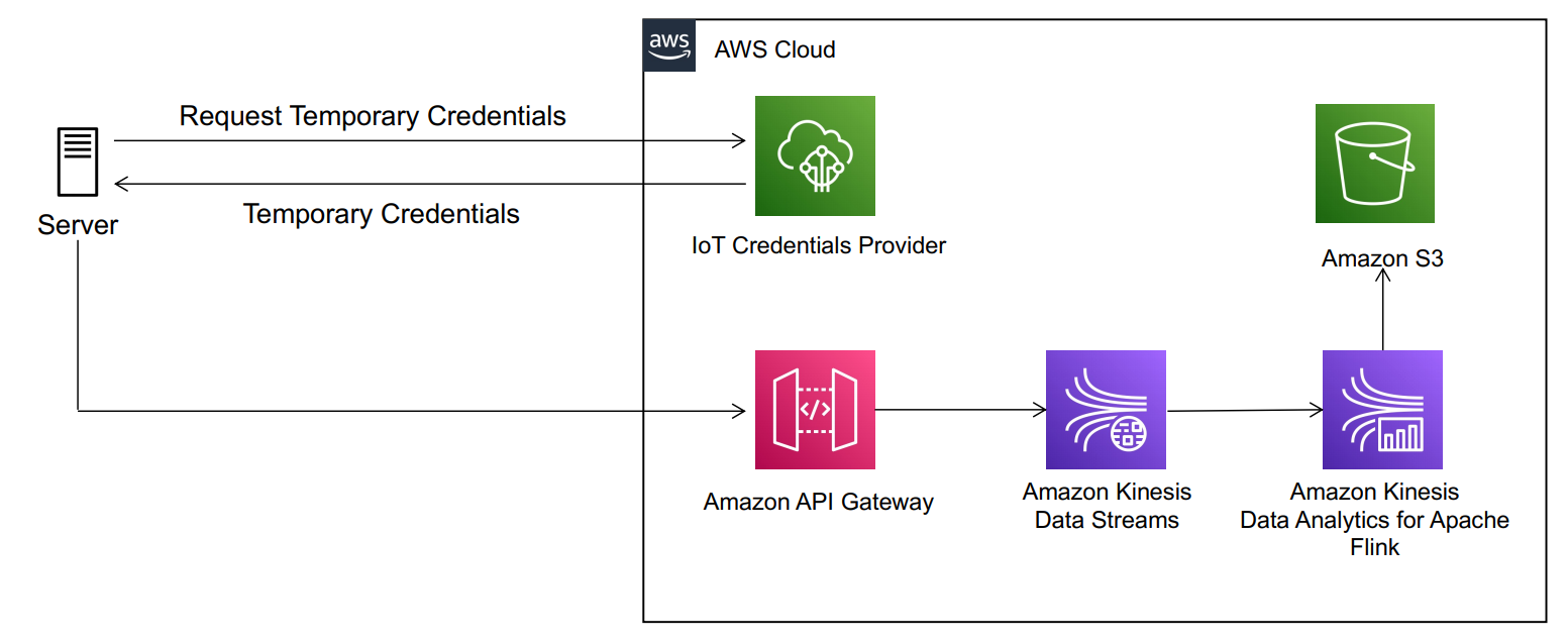
The following architecture diagram illustrates the data ingestion pipeline.

In this architecture, authorized servers from one or multiple third-party companies send messages to an API Gateway endpoint. The endpoint puts messages into the proper partition of a shared Kinesis data stream. Finally, a Kinesis Data Analytics consumer application aggregates, compresses, and writes data into the proper partition of an S3 data lake.

The following sections describe in more detail the multi-tenant architecture considerations and implementation details for this architecture.

Authentication

First, you need to decide on the desired authentication mechanisms. To simplify onboarding new customers and eliminate the need for hardcoded credentials on customers servers, we recommend looking into the credentials provider feature of AWS IoT. Each tenant can use a provisioned x.509 certificate to securely retrieve temporary credentials and authenticate against AWS services using an AWS Identity and Access Management (IAM) role. For more information on how this works, see How to Eliminate the Need for Hardcoded AWS Credentials in Devices by Using the AWS IoT Credentials Provider.

For additional authentication mechanisms directly with API Gateway, see Controlling and managing access to a REST API in API Gateway.

Authorization

After you’re authenticated with IAM, the next step is authorization. Simply put, make sure each tenant can only write to their respective data lake partition. One of the key risks to mitigate in a multi-tenant steaming ingestion workflow is the scenario where a tenant server is compromised and it attempts to impersonate other tenants sending bogus data. To guarantee isolation of data ingest and reduce the blast radius of bad data, you could consider the following options:

  • Use a silo model and provision one Kinesis data stream per tenant – Kinesis Data Streams provides access control at the stream level. This approach provides you with complete isolation and the ability to scale your stream capacity up or down on a per-tenant basis. However, there is operational overhead in maintaining multiple streams, and optimizing for cost has limitations. Each data stream is provisioned by increments of one shard or 1 MB/sec of ingestion capacity with up to 1,000 PUT records per second. Pricing is based on shards per hour. One shard could be well beyond your tenant requirements and tenant onboarding costs could scale rapidly.
  • Use AWS IoT Core with one topic per tenant using topic filters and an AWS IoT rule to push data into a shared data streamAWS IoT Core gives access control at the topic level. Each tenant can send data to only their respective topic (for example, tenantID topic) based on their IAM credentials. We can then use an AWS IoT rule to extract the tenantID from the topic and push data into a shared data stream using tenantID as the partition key.
  • Use API Gateway as a proxy with mapping templates and a shared data stream – Kinesis Data Streams doesn’t provide access control at the data partition level. However, API Gateway provides access control at the method and path level. With API Gateway as a proxy, you can use mapping templates to programmatically fetch the tenant UUID from the path and set it as the partition key before pushing the data to Kinesis Data Streams.

Optimize for costs

The last two preceding options use a pool model and share a single Kinesis data stream to reduce operational overhead and costs. To optimize costs even further, you need to consider the pricing model of each of these services (API Gateway vs. AWS IoT Core) and three factors in your use case: the average size for each message, the rate at which the data is being ingested, and the data latency requirements.

Consider an example where you have 1,000 tenants (devices) and each produces data at the rate of one request per second with an average payload of 8 KB. AWS IoT Core is priced per million messages and per million rules. Each message is metered at 5 KB increments, so you’re charged for two messages per payload. If you have small payloads and very low latency requirements, AWS IoT Core is likely your best choice. If you can introduce some latency and buffer your messages at each tenant, then API Gateway is your best option because the pricing model for REST APIs requests is on a per-API call basis and not metered by KB. You can use the AWS Pricing Calculator to quickly decide which option offers the best price for your use case.

For example, with API Gateway, you can optimize your cost even further by reducing the number of API requests. Instead of each tenant sending 8 KB of data per second, you can send 240 KB every 30 seconds and reduce costs considerably. We can explore a sample cost calculation for API Gateway considering this scenario: average size of message: 240 KB, REST API request units per month: 2 request per minute x 60 min x 24 hrs. x 30 days = 86,400 requests x 1,000 tenants = 86,400,000.

The following sections walk you through the configuration of API Gateway and Kinesis to prevent cross-data access when you support a multi-tenant streaming ingestion pipeline architecture.

Enable API Gateway as a Kinesis Data Streams proxy

API Gateway is a fully managed service that makes it easy for developers to publish, maintain, monitor, and secure APIs at any scale. You can create an API Gateway endpoint to expose other AWS services, such as Amazon Simple Notification Service (Amazon SNS), Amazon S3, Kinesis, and even AWS Lambda. All AWS services support dedicated APIs to expose their features. However, the application protocols or programming interfaces are likely to differ from service to service. An API Gateway API with the AWS integration has the advantage of providing a consistent application protocol for your client to access different AWS services. In our use case, we use API Gateway as a proxy to Kinesis in order to handle IAM authentication and authorize clients to invoke URL paths with their unique tenant ID. API Gateway has additional features that are beneficial for multi-tenant applications, like rate limiting API calls per tenant, requests and response transformations, logging and monitoring, and more.

When you configure API Gateway with IAM resource-level permissions, you can make sure each tenant can only make requests to a unique URL path. For example, if the tenant invokes the API Gateway URL with their tenant ID in the path (for example, https://api-id.execute-api.us-east-2.amazonaws.com/{tenantId}), IAM validates that the tenant is authorized to invoke this URL only. For more details on how to set up an IAM policy to a specific API Gateway URL path, see Control access for invoking an API.

Then, to ensure no authorized customer can impersonate other tenant by sending bogus data, API Gateway extracts the tenant ID from the URL path programmatically using the API Gateway mapping template feature. API Gateway allows developers to transform payloads before passing it to backend resources using mapping templates written with JSONPath expressions. With this feature, we can extract the tenant ID from the URL and pass it as the partition key of the shared data stream. The following is a sample mapping template:

{
    "StreamName": "$input.params('stream-name')",
    "Data": "$util.base64Encode($input.json('$.Data'))",
    "PartitionKey": "$input.params('partition')"
}

In the preceding code, partition is the parameter name you specify in your API Gateway resource path. The following screenshot shows what the configuration looks like on the API Gateway console.

After messages in the data stream use the proper partition, the next step is to transform, enrich, and aggregate messages before writing them into an S3 data lake. For this workflow, we use Kinesis Data Analytics for Apache Flink to have full control of the data lake partition configuration. The following section describes the approach to ensure data is written in the proper partition.

Use Kinesis Data Analytics for Apache Flink to process and write data into an S3 data lake

After we guarantee that messages within the data stream have the right tenant ID as the partition key, we can use Kinesis Data Analytics for Apache Flink to continuously process messages in near-real time and store them in Amazon S3. Kinesis Data Analytics for Apache Flink is an easy way to transform and analyze streaming data in real time. Apache Flink is an open-source framework and engine for processing data streams. Kinesis Data Analytics reduces the complexity of building, managing, and integrating Apache Flink applications with other AWS services. Because this solution is also serverless, there are no servers to manage, it scales automatically to match the volume and throughput of your incoming data, and you only pay for the resources your streaming applications consume.

In this scenario, we want to extract the partition key (tenantId) from each Kinesis data stream message, then process all messages within a time window and use the tenant ID as the file prefix of the files we write into the destination S3 bucket. In other words, we write the data into the proper tenant partition. The result writes data in files that look like the following:

s3://mybucket/year=2020/month=1/day=1/tenant=A01/part-0-0
s3://mybucket/year=2020/month=1/day=1/tenant=A02/part-0-1
s3://mybucket/year=2020/month=1/day=1/tenant=A03/part-0-3

To achieve this, we need to implement two custom classes within the Apache Flink application code.

First, we use a custom deserializer class to extract the partition key from the data stream and append it to the body of the message. We can achieve this by overriding the deserialize method of the KinesisDeserializationSchema class:

class CustomKinesisDeserializer implements  KinesisDeserializationSchema<String> {
    private static final Logger log = LogManager.getLogger(CustomKinesisDeserializer.class);
   @Override
    public String deserialize(byte[] bytes, String partitionKey, String seqNum,
                              long approxArrivalTimeStamp, String stream, String shardId) throws IOException {
        log.debug("deserialize - enter");
        String s = new String(bytes);
        JSONObject json = new JSONObject(s);
        json.put("tenantid", partitionKey);
        return json.toString();
    }
    @Override
    public TypeInformation<String> getProducedType() {
        return BasicTypeInfo.STRING_TYPE_INFO;
    }
}

Next, we use a customBucketAssignerclass to use the partition key in the body of the message (in our case, the tenant ID) as the bucket prefix:

private static final BucketAssigner<String, String> assigner = new BucketAssigner<String, String> () {

        @Override
        public String getBucketId(String element, BucketAssigner.Context context) {
            log.debug("getBucketId - enter");
            JSONObject json = new JSONObject(element);
            if (json.has("tenantid")) {
                String tenantId = json.getString("tenantid");
                return "tenantid=" + tenantId;
            }
            return "tenantid=unknown";
        }

        @Override
        public SimpleVersionedSerializer<String> getSerializer() {
            return SimpleVersionedStringSerializer.INSTANCE;
        }
};

The following code is the full sample class for the Kinesis Data Analytics with Apache Flink application. The purpose of the sample code is to illustrate how you can obtain the partition key from the data stream and use it as your bucket prefix via the BucketAssigner class. Your implementation might require additional windowing logic to enrich, aggregate, and transform your data before writing it into an S3 bucket. In this post, we write data into a tenantId partition, but your code might require additional partition fields (such as by date). For additional code examples, see Kinesis Data Analytics for Apache Flink: Examples.

package com.amazonaws.services.kinesisanalytics;

import com.amazonaws.services.kinesisanalytics.runtime.KinesisAnalyticsRuntime;
import org.apache.flink.api.common.serialization.SimpleStringEncoder;
import org.apache.flink.api.common.typeinfo.TypeInformation;
import org.apache.flink.core.fs.Path;
import org.apache.flink.core.io.SimpleVersionedSerializer;
import org.apache.flink.streaming.api.datastream.DataStream;
import org.apache.flink.streaming.api.environment.StreamExecutionEnvironment;
import org.apache.flink.streaming.api.functions.sink.filesystem.BucketAssigner;
import org.apache.flink.streaming.api.functions.sink.filesystem.StreamingFileSink;
import org.apache.flink.streaming.api.functions.sink.filesystem.bucketassigners.SimpleVersionedStringSerializer;
import org.apache.flink.streaming.connectors.kinesis.FlinkKinesisConsumer;
import org.apache.flink.streaming.connectors.kinesis.config.ConsumerConfigConstants;
import org.apache.flink.streaming.connectors.kinesis.serialization.KinesisDeserializationSchema;
import org.apache.logging.log4j.LogManager;
import org.apache.logging.log4j.Logger;
import org.json.JSONObject;

import java.io.IOException;
import java.util.Map;
import java.util.Properties;

public class S3StreamingSinkWithPartitionsJob {

    private static final Logger log = LogManager.getLogger(S3StreamingSinkWithPartitionsJob.class);
    private static String s3SinkPath;
    private static String inputStreamName;
    private static String region;

    /**
     * Custom BucketAssigner to specify the bucket path/prefix with the Kinesis Stream partitionKey.
     *
     * Sample code. Running application with debug mode with this implementation will expose data into log files
     */
    private static final BucketAssigner<String, String> assigner = new BucketAssigner<String, String> () {

        @Override
        public String getBucketId(String element, BucketAssigner.Context context) {
            log.debug("getBucketId - enter");
            JSONObject json = new JSONObject(element);
            if (json.has("tenantid")) {
                String tenantId = json.getString("tenantid");
                return "tenantid=" + tenantId;
            }
            return "tenantid=unknown";
        }

        @Override
        public SimpleVersionedSerializer<String> getSerializer() {
            return SimpleVersionedStringSerializer.INSTANCE;
        }
    };


    private static DataStream<String> createSourceFromStaticConfig(StreamExecutionEnvironment env) throws IOException {
        log.debug("createSourceFromStaticConfig - enter - variables: {region:" + region +
                ", inputStreamName:" + inputStreamName + "}");
        Properties inputProperties = new Properties();
        inputProperties.setProperty(ConsumerConfigConstants.AWS_REGION, region);
        inputProperties.setProperty(ConsumerConfigConstants.STREAM_INITIAL_POSITION, "LATEST");

        /*
         * Implementinga custom serializer class that extends KinesisDeserializationSchema interface
         * to get additional values from partition keys.
         */
        return env.addSource(new FlinkKinesisConsumer<>(inputStreamName,
                new CustomKinesisDeserializer(),
                inputProperties
        ));
    }

    private static StreamingFileSink<String> createS3SinkFromStaticConfig() {
        log.debug("createS3SinkFromStaticConfig - enter - variables: { s3SinkPath:" + s3SinkPath + "}");
        final StreamingFileSink<String> sink = StreamingFileSink
                .forRowFormat(new Path(s3SinkPath), new SimpleStringEncoder<String>("UTF-8"))
                .withBucketAssigner(assigner)
                .build();
        return sink;
    }

    public static void main(String[] args) throws Exception {

        Map<String, Properties> applicationProperties = KinesisAnalyticsRuntime.getApplicationProperties();
        Properties consumerProperties = applicationProperties.get("ConsumerConfigProperties");
        region = consumerProperties.getProperty("Region","us-west-2");
        inputStreamName = consumerProperties.getProperty("InputStreamName");
        s3SinkPath = "s3a://" + consumerProperties.getProperty("S3SinkPath") + "/data";

        final StreamExecutionEnvironment env = StreamExecutionEnvironment.getExecutionEnvironment();
        DataStream<String> input = createSourceFromStaticConfig(env);
        input.addSink(createS3SinkFromStaticConfig());
        env.execute("Flink S3 Streaming with Partitions Sink Job");
    }

}

/**
 * Custom deserializer to pass partitionKey from KDS into the record value. The partition key can be used
 * by the bucket assigner to leverage it as the s3 path/prefix/partition.
 *
 * Sample code. Running application with debug mode with this implementation will expose data into log files
 */

class CustomKinesisDeserializer implements  KinesisDeserializationSchema<String> {

    private static final Logger log = LogManager.getLogger(CustomKinesisDeserializer.class);

    @Override
    public String deserialize(byte[] bytes, String partitionKey, String seqNum,
                              long approxArrivalTimeStamp, String stream, String shardId) throws IOException {
        log.debug("deserialize - enter");
        String s = new String(bytes);
        JSONObject json = new JSONObject(s);
        json.put("tenantid", partitionKey);
        return json.toString();
    }

    @Override
    public TypeInformation<String> getProducedType() {
        return TypeInformation.of(String.class);
    }

}

To test and build this multi-tenant stream ingestion pipeline, you can deploy an AWS CloudFormation template in your AWS environment. The following section provides step-by-step instructions on how to deploy and test the sample template.

Deploy a sample multi-tenant streaming ingestion pipeline

AWS CloudFormation simplifies provisioning and managing infrastructure and services on AWS via JSON or .yaml templates. Follow these instructions to deploy and test the sample workflow described in this post. The instructions assume a basic understanding of AWS Cloud concepts, the AWS Management Console, and working with REST APIs.

  1. Create a destination S3 bucket.
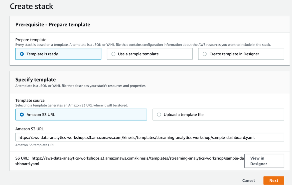
  2. Deploy the CloudFormation template.

The template has only been tested in the us-west-2 Region, and creates IAM roles and users with limited access scope. This template doesn’t register CA certificates or implement the AWS IoT credentials provider feature for authentication. To test the pipeline, the template creates an IAM user for authentication with API Gateway. If you want to test the AWS IoT credentials provider feature with this implementation, follow the instructions in How to Eliminate the Need for Hardcoded AWS Credentials in Devices by Using the AWS IoT Credentials Provider.

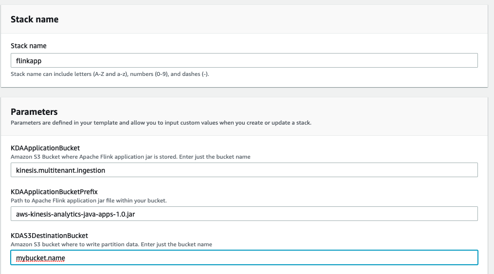
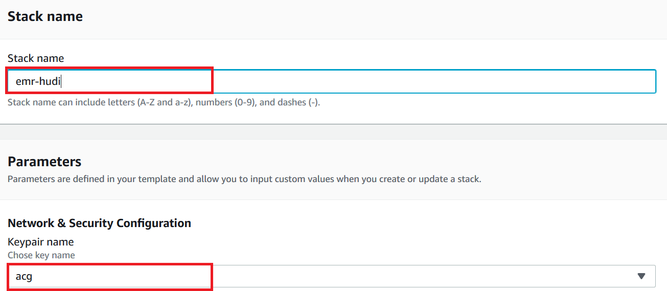
  1. For Stack name¸ enter a name (for example, flinkapp).
  2. For KDAS3DestinationBucket, enter the name of the S3 bucket you created.
  3. Leave the other parameters as default.

  1. Accept all other options, including acknowledging the template will create IAM principals on your behalf.
  2. Wait until the stack shows the status CREATE_COMPLETE.

Now you can start your Kinesis Data Analytics for Apache Flink application.

  1. On the Kinesis Data Analytics console, choose Analytics applications.
  2. Select the application that starts with KinesisAnalyticsFI_*.
  3. Choose Run.

  1. Choose Run without snapshot.
  2. Wait for the application to show the status Running.

Now you can test sending messages to your API Gateway endpoint. Remember requests should be authenticated. The CloudFormation template created an IAM test user for this purpose. We recommend using a development API tool for this step. For this post, we use Postman.

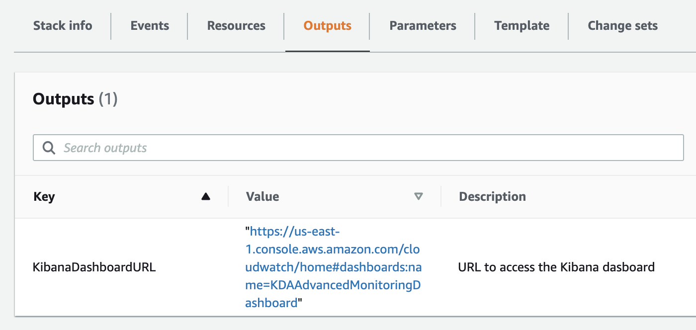
  1. On the AWS CloudFormation console, navigate to the Outputs tab of your stack.
  2. Note the API Gateway endpoint (InvokeURL) and the name of the IAM test user.

  1. Create and retrieve the access key and secret key of your test user. For instructions, see Programmatic access.

AWS recommends using temporary keys when authenticating requests to AWS services. For testing purposes, we use a long-lived access key from this limited scope test user.

  1. Use your API development tool to build a POST request to your API Gateway endpoint using your IAM test user secrets.

The following screenshot shows the Authorization tab of the request using Postman.

The following screenshot shows the Body tab of the request using Postman.

  1. For the body of the request, you can use the following payload:
{
    Data: {
        "key1": "value1",
        "key2": "value2",
        "key3": "value3"
    }
}

You should get a response from the data stream that looks as follows:

{
 "EncryptionType": "KMS",
 "SequenceNumber": "49619151594519161991565402527623825830782609999622307842",
 "ShardId": "shardId-000000000000"
}

  1. Try to make a request to a different tenant by changing the path from /prod/T001 to /prod/T002.

Because the user isn’t authorized to send data to this endpoint, you get the following error message:

{
    "Message": "User: arn:aws:iam::*******4205:user/flinkapp-MultiTenantStreamTestUser-EWUSMWR0T5I5 is not authorized to perform: execute-api:Invoke on resource: arn:aws:execute-api:us-west-2:********4205:fktw02penb/prod/POST/T002"
}

  1. Browse to your destination S3 bucket.

You should be able to see a new file within your T001 tenant’s folder or partition.

  1. Download and open your file (part-*-*).

The content should look like the following data (in this scenario, we made six requests to the tenant’s API Gateway endpoint):

{"key1":"value1","key2":"value2","key3":"value3","tenantid":"T001"}

Clean up

After you finalize your testing, delete the CloudFormation stack and any data written into your destination S3 bucket to prevent incurring unnecessary charges.

Conclusion

Sharing resources in multi-tenant architectures allows organizations to optimize for costs while providing controls for proper tenant isolation and security. In this post, we showed you how to use API Gateway as a proxy to authorize tenants to a specific partition in your shared Kinesis data stream and prevent cross-tenant data access when performing data ingestion from semi-trusted servers. We also showed you how buffering data and sharing a single data stream with multiple tenants reduces operational overhead and optimizes for costs by taking advantage of better resource utilization. Check out the Kinesis Data Streams and Kinesis Data Analytics quick starts to evaluate them for your multi-tenant ingestion use case.


About the Authors

Abhinav Krishna Vadlapatla is a Solutions Architect with Amazon Web Services. He supports startups and small businesses with their cloud adoption to build scalable and secure solutions using AWS. In his free time, he likes to cook and travel.


Pablo Redondo Sanchez is a Senior Solutions Architect at Amazon Web Services. He is a data enthusiast and works with customers to help them achieve better insights and faster outcomes from their data analytics workflows. In his spare time, Pablo enjoys woodworking and spending time outdoor with his family in Northern California.

Query a Teradata database using Amazon Athena Federated Query and join with data in your Amazon S3 data lake

Post Syndicated from Navnit Shukla original https://aws.amazon.com/blogs/big-data/query-a-teradata-database-using-amazon-athena-federated-query-and-join-with-data-in-your-amazon-s3-data-lake/

If you use data lakes in Amazon Simple Storage Service (Amazon S3) and use Teradata as your transactional data store, you may need to join the data in your data lake with Teradata in the cloud, Teradata running on Amazon Elastic Compute Cloud (Amazon EC2), or with an on-premises Teradata database, for example to build a dashboard or create consolidated reporting.

In these use cases, the Amazon Athena Federated Query feature allows you to seamlessly access the data from Teradata database without having to move the data to your S3 data lake. This removes the overhead in managing such jobs.

In this post, we will walk you through a step-by-step configuration to set up Athena Federated Query using AWS Lambda to access data in a Teradata database running on premises.

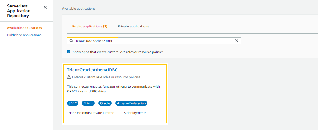
For this post, we will be using the Oracle Athena Federated Query connector developed by Trianz. The runtime includes a Teradata instance on premises. Your Teradata instance can be on the cloud, on Amazon EC2, or on premises. You can deploy the Trianz Oracle Athena Federated Query connector from the AWS Serverless Application Repository.

Let’s start with discussing the solution and then detailing the steps involved.

Solution overview

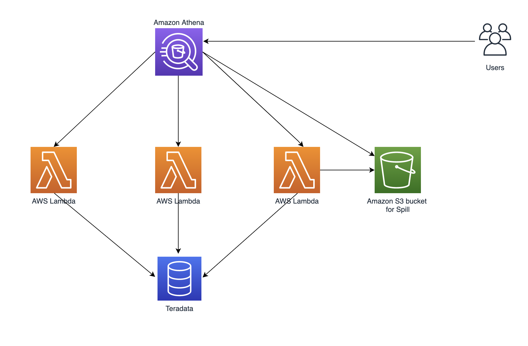
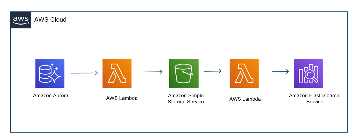
Data federation is the capability to integrate data in another data store using a single interface (Athena). The following diagram depicts how Athena Federated Query works by using Lambda to integrate with a federated data source.

Athena is an interactive query service that makes it easy to analyze data in Amazon S3 using standard SQL. If you have data in sources other than Amazon S3, you can use Athena Federated Query to query the data in place or build pipelines to extract data from multiple data sources and store them in Amazon S3. With Athena Federated Query, you can run SQL queries across data stored in relational, non-relational, object, and custom data sources.

When a federated query is run, Athena identifies the parts of the query that should be routed to the data source connector and executes them with Lambda. The data source connector makes the connection to the source, runs the query, and returns the results to Athena. If the data doesn’t fit into Lambda RAM runtime memory, it spills the data to Amazon S3 and is later accessed by Athena.

Athena uses data source connectors which internally use Lambda to run federated queries. Data source connectors are pre-built and can be deployed from the Athena console or from the Serverless Application Repository. Based on the user submitting the query, connectors can provide or restrict access to specific data elements.

To implement this solution, we complete the following steps:

  1. Create a secret for the Teradata instance using AWS Secrets Manager.
  2. Create an S3 bucket and subfolder for Lambda to use.
  3. Configure Athena federation with the Teradata instance.
  4. Run federated queries with Athena.

Prerequisite

Before you start this walkthrough, make sure your Teradata database is up and running.

Create a secret for the Teradata instance

Our first step is to create a secret for the Teradata instance with a username and password using Secrets Manager.

  1. On the Secrets Manager console, choose Secrets.
  2. Choose Store a new secret.
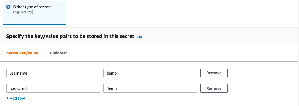
  3. Select Other types of secrets.
  4. Set the credentials as key-value pairs (username, password) for your Teradata instance.

  1. For Secret name, enter a name for your secret. Use the prefix TeradataAFQ so it’s easy to find.
  2. Leave the remaining fields at their defaults and choose Next.
  3. Complete your secret creation.

Set up your S3 bucket for Lambda

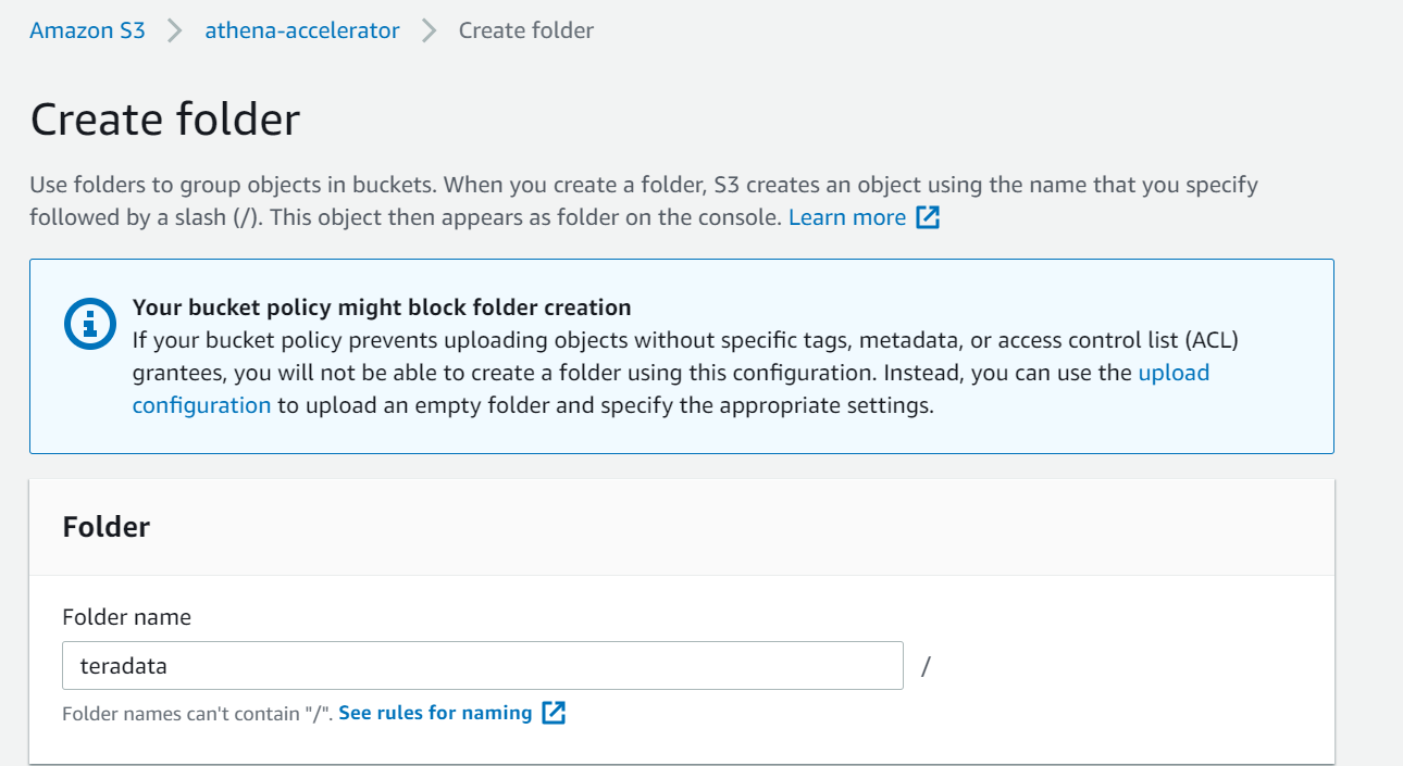
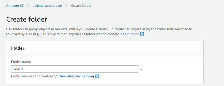
On the Amazon S3 console, create a new S3 bucket and subfolder for Lambda to use. For this post, we create athena-accelerator/teradata.

Configure Athena federation with the Teradata instance

To configure Athena federation with Teradata instance, complete the following steps:

  1. On the AWS Serverless Application Repository console, choose Available applications.
  2. Select Show apps that create custom IAM roles or resource policies.
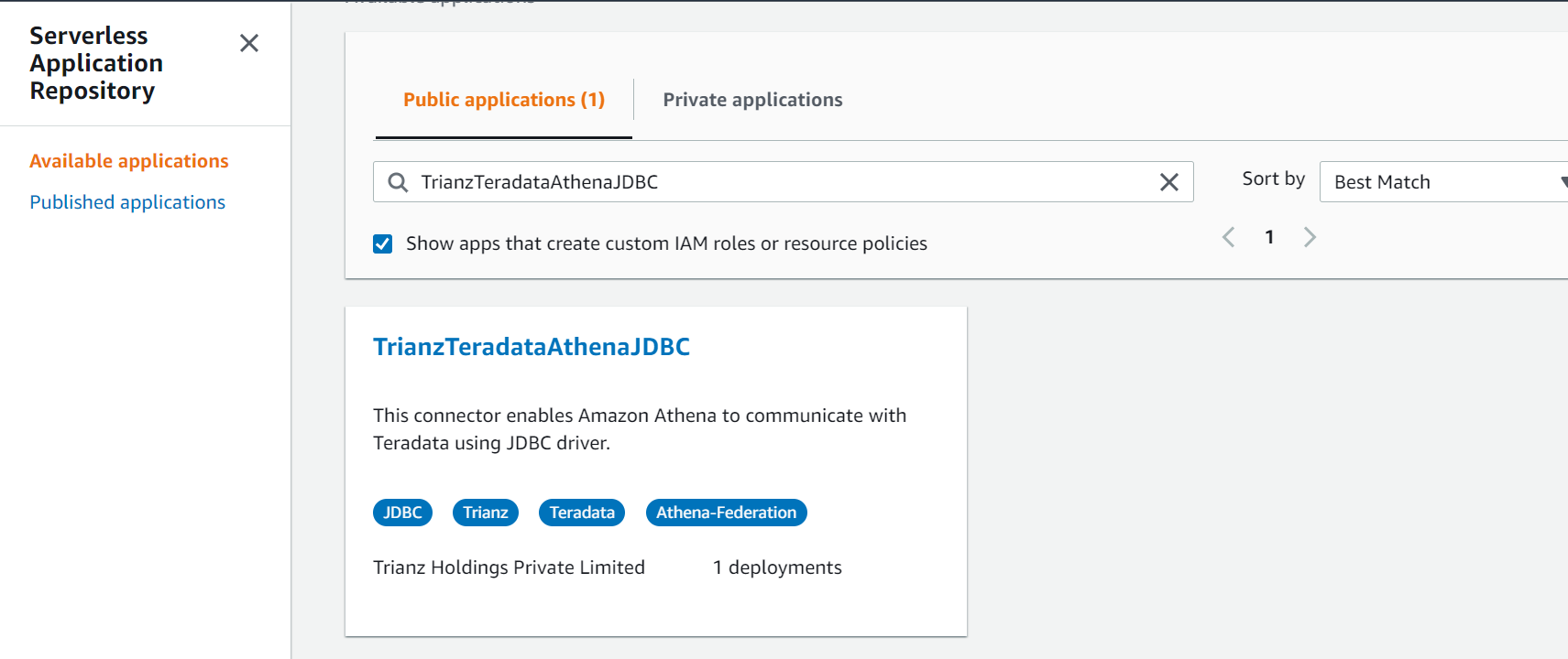
  3. In the search field, enter TrianzTeradataAthenaJDBC.
  4. Choose the application.

  1. For SecretNamePrefix, enter TeradataAFQ.
  2. For SpillBucket, enter Athena-accelerator/teradata.
  3. For JDBCConnectorConfig, use the format teradata://jdbc:teradata://hostname/user=testUser&password=testPassword.
  4. For DisableSpillEncryption, enter false.
  5. For LambdaFunctionName, enter teradataconnector.
  6. For SecurityGroupID, enter the security group ID where the Teradata instance is deployed.

Make sure to apply valid inbound and outbound rules based on your connection.

  1. For SpillPrefix, create a folder under the S3 bucket you created and specify the name (for example, athena-spill).
  2. For Subnetids, use the subnets where the Teradata instance is running with comma separation.

Make sure the subnet is in a VPC and has NAT gateway and internet gateway attached.

  1. Select the I acknowledge check box.
  2. Choose Deploy.

Make sure that the AWS Identity and Access Management (IAM) roles have permissions to access AWS Serverless Application Repository, AWS CloudFormation, Amazon S3, Amazon CloudWatch, Amazon CloudTrail, Secrets Manager, Lambda, and Athena. For more information about Athena IAM access, see Example IAM Permissions Policies to Allow Athena Federated Query.

Run federated queries with Athena

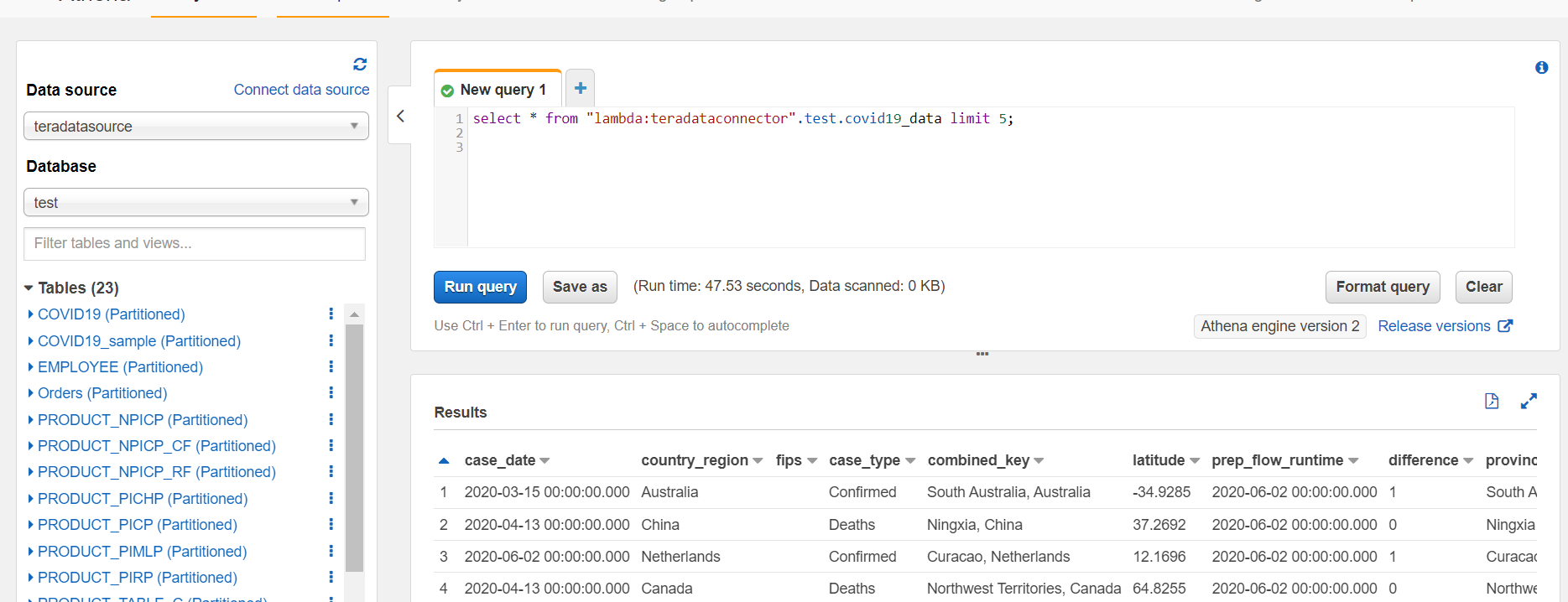
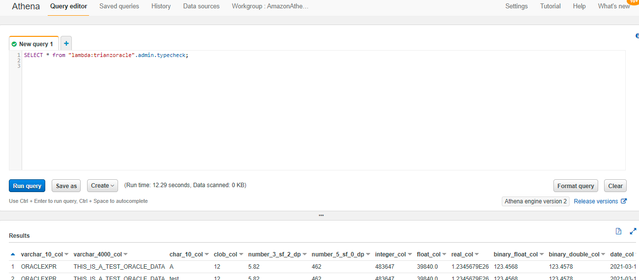
Run your queries using lambda:teradataconnector to run against tables in the Teradata database. teradataconnector is the name of lambda function which we have created in step 7 of previous section of this blog.

lambda:teradataconnector references a data source connector Lambda function using the format lambda:MyLambdaFunctionName. For more information, see Writing Federated Queries.

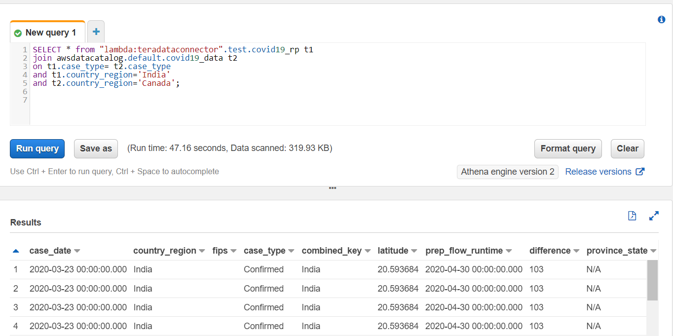
The following screenshot shows the query that joins the dataset between Teradata and the S3 data lake.

Key performance best practices

If you’re considering Athena Federated Query with Teradata, we recommend the following best practices:

  • Athena Federated query works great for queries with predicate filtering because the predicates are pushed down to the Teradata database. Use filter and limited-range scans in your queries to avoid full table scans.
  • If your SQL query requires returning a large volume of data from the Teradata database to Athena (which could lead to query timeouts or slow performance), you may consider moving data from Teradata to your S3 data lake.
  • The star schema is a commonly used data model in Teradata. In the star schema model, unload your large fact tables into your S3 data lake and leave the dimension tables in Teradata. If large dimension tables are contributing to slow performance or query timeouts, unload those tables to your S3 data lake.
  • When you run federated queries, Athena spins up multiple Lambda functions, which causes a spike in database connections. It’s important to monitor the Teradata database WLM queue slots to ensure there is no queuing. Additionally, you can use concurrency scaling on your Teradata database cluster to benefit from concurrent connections to queue up.

Conclusion

In this post, you learned how to configure and use Athena Federated Query with Teradata. Now you don’t need to wait for all the data in your Teradata data warehouse to be unloaded to Amazon S3 and maintained on a day-to-day basis to run your queries.

You can use the best practices outlined in the post to help minimize the data transferred from Teradata for better performance. When queries are well written for Athena Federated Query, the performance penalties are negligible.

For more information, see the Athena User Guide and Using Amazon Athena Federated Query.


About the Author

Navnit Shukla is an AWS Specialist Solution Architect in Analytics. He is passionate about helping customers uncover insights from their data. He has been building solutions to help organizations make data-driven decisions.

Query an Apache Hudi dataset in an Amazon S3 data lake with Amazon Athena part 1: Read-optimized queries

Post Syndicated from Dhiraj Thakur original https://aws.amazon.com/blogs/big-data/part-1-query-an-apache-hudi-dataset-in-an-amazon-s3-data-lake-with-amazon-athena-part-1-read-optimized-queries/

On July 16, 2021, Amazon Athena upgraded its Apache Hudi integration with new features and support for Hudi’s latest 0.8.0 release. Hudi is an open-source storage management framework that provides incremental data processing primitives for Hadoop-compatible data lakes. This upgraded integration adds the latest community improvements to Hudi along with important new features including snapshot queries, which provide near real-time views of table data, and reading bootstrapped tables which provide efficient migration of existing table data.

In this series of posts on Athena and Hudi, we will provide a short overview of key Hudi capabilities along with detailed procedures for using read-optimized queries, snapshot queries, and bootstrapped tables.

Overview

With Apache Hudi, you can perform record-level inserts, updates, and deletes on Amazon S3, allowing you to comply with data privacy laws, consume real-time streams and change data captures, reinstate late-arriving data, and track history and rollbacks in an open, vendor neutral format. Apache Hudi uses Apache Parquet and Apache Avro storage formats for data storage, and includes built-in integrations with Apache Spark, Apache Hive, and Apache Presto, which enables you to query Apache Hudi datasets using the same tools that you use today with near-real-time access to fresh data.

An Apache Hudi dataset can be one of the following table types:

  • Copy on Write (CoW) – Data is stored in columnar format (Parquet), and each update creates a new version of the base file on a write commit. A CoW table type typically lends itself to read-heavy workloads on data that changes less frequently.
  • Merge on Read (MoR) – Data is stored using a combination of columnar (Parquet) and row-based (Avro) formats. Updates are logged to row-based delta files and are compacted as needed to create new versions of the columnar files. A MoR table type is typically suited for write-heavy or change-heavy workloads with fewer reads.

Apache Hudi provides three logical views for accessing data:

  • Read-optimized – Provides the latest committed dataset from CoW tables and the latest compacted dataset from MoR tables
  • Incremental – Provides a change stream between two actions out of a CoW dataset to feed downstream jobs and extract, transform, load (ETL) workflows
  • Real-time – Provides the latest committed data from a MoR table by merging the columnar and row-based files inline

As of this writing, Athena supports read-optimized and real-time views.

Using read-optimized queries

In this post, you will use Athena to query an Apache Hudi read-optimized view on data residing in Amazon S3. The walkthrough includes the following high-level steps:

  1. Store raw data in an S3 data lake.
  2. Transform the raw data to Apache Hudi CoW and MoR tables using Apache Spark on Amazon EMR.
  3. Query and analyze the tables on Amazon S3 with Athena on a read-optimized view.
  4. Perform an update to a row in the Apache Hudi dataset.
  5. Query and analyze the updated dataset using Athena.

Architecture

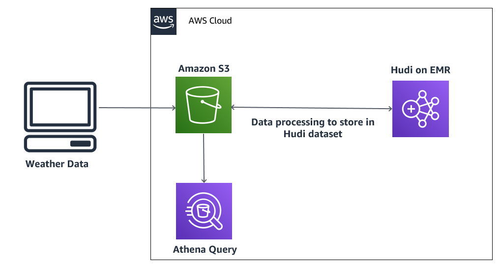
The following diagram illustrates our solution architecture.

In this architecture, you have high-velocity weather data stored in an S3 data lake. This raw dataset is processed on Amazon EMR and stored in an Apache Hudi dataset in Amazon S3 for further analysis by Athena. If the data is updated, Apache Hudi performs an update on the existing record, and these updates are reflected in the results fetched by the Athena query.

Let’s build this architecture.

Prerequisites

Before getting started, we set up our resources. For this post, we use the us-east-1 Region.

  1. Create an Amazon Elastic Compute Cloud (Amazon EC2) key pair. For instructions, see Create a key pair using Amazon EC2.
  2. Create a S3 bucket for storing the raw weather data (for this post, we call it weather-raw-bucket).
  3. Create two folders in the S3 bucket: parquet_file and delta_parquet.
  4. Download all the data files, Apache Scala scripts (data_insertion_cow_delta_script, data_insertion_cow_script, data_insertion_mor_delta_script, and data_insertion_mor_script), and Athena DDL code (athena_weather_hudi_cow.sql and athena_weather_hudi_mor.sql) from the GitHub repo.
  5. Upload the weather_oct_2020.parquet file to weather-raw-bucket/parquet_file.
  6. Upload the file weather_delta.parquet to weather-raw-bucket/delta_parquet. We update an existing weather record from a relative_humidity of 81 to 50 and a temperature of 6.4 to 10.
  7. Create another S3 bucket for storing the Apache Hudi dataset. For this post, we create a bucket with a corresponding subfolder named athena-hudi-bucket/hudi_weather.
  8. Deploy the EMR cluster using the provided AWS CloudFormation template:
  9. Enter a name for your stack.
  10. Choose a pre-created key pair name.

This is required to connect to the EMR cluster nodes. For more information, see Connect to the Master Node Using SSH.

  1. Accept all the defaults and choose Next.
  2. Acknowledge that AWS CloudFormation might create AWS Identity and Access Management (IAM) resources.
  3. Choose Create stack.

Use Apache Hudi with Amazon EMR

When the cluster is ready, you can use the provided key pair to SSH into the primary node.

  1. Use the following bash command to load the spark-shell to work with Apache Hudi:
    spark-shell --conf "spark.serializer=org.apache.spark.serializer.KryoSerializer" --conf "spark.sql.hive.convertMetastoreParquet=false" --jars /usr/lib/hudi/hudi-spark-bundle.jar,/usr/lib/spark/external/lib/spark-avro.jar

  2. On the spark-shell, run the following Scala code in the script data_insertion_cow_script to import weather data from the S3 data lake to an Apache Hudi dataset using the CoW storage type:
    import org.apache.spark.sql.SaveMode
    import org.apache.spark.sql.functions._
    import org.apache.hudi.DataSourceWriteOptions
    import org.apache.hudi.config.HoodieWriteConfig
    import org.apache.hudi.hive.MultiPartKeysValueExtractor
    
    //Set up various input values as variables
    val inputDataPath = "s3://weather-raw-bucket/parquet_file/"
    val hudiTableName = "weather_hudi_cow"
    val hudiTablePath = "s3://athena-hudi-bucket/hudi_weather/" + hudiTableName
    
    // Set up our Hudi Data Source Options
    val hudiOptions = Map[String,String](
        DataSourceWriteOptions.RECORDKEY_FIELD_OPT_KEY -> "city_id",
    	DataSourceWriteOptions.RECORDKEY_FIELD_OPT_KEY -> "timestamp",
        DataSourceWriteOptions.PARTITIONPATH_FIELD_OPT_KEY -> "date", 
        HoodieWriteConfig.TABLE_NAME -> hudiTableName, 
        DataSourceWriteOptions.OPERATION_OPT_KEY ->
            DataSourceWriteOptions.INSERT_OPERATION_OPT_VAL, 
        DataSourceWriteOptions.PRECOMBINE_FIELD_OPT_KEY -> "timestamp", 
        DataSourceWriteOptions.HIVE_SYNC_ENABLED_OPT_KEY -> "true", 
        DataSourceWriteOptions.HIVE_TABLE_OPT_KEY -> hudiTableName, 
        DataSourceWriteOptions.HIVE_PARTITION_FIELDS_OPT_KEY -> "date", 
        DataSourceWriteOptions.HIVE_PARTITION_EXTRACTOR_CLASS_OPT_KEY ->
            classOf[MultiPartKeysValueExtractor].getName)
    
    // Read data from S3 and create a DataFrame with Partition and Record Key
    val inputDF = spark.read.format("parquet").load(inputDataPath)
    
    // Write data into the Hudi dataset
    inputDF.write.format("org.apache.hudi").options(hudiOptions).mode(SaveMode.Append).save(hudiTablePath)

Replace the S3 bucket path for inputDataPath and hudiTablePath in the preceding code with your S3 bucket.

For more information about DataSourceWriteOptions, see Work with a Hudi Dataset.

  1. In the spark-shell, count the total number of records in the Apache Hudi dataset:
    scala> inputDF.count()
    res1: Long = 1000

  2. Repeat the same step for creating an MoR table using data_insertion_mor_script (the default is COPY_ON_WRITE).
  3. Run the spark.sql("show tables").show(); query to list three tables, one for CoW and two queries, _rt and _ro, for MoR.

The following screenshot shows our output.

Let’s check the processed Apache Hudi dataset in the S3 data lake.

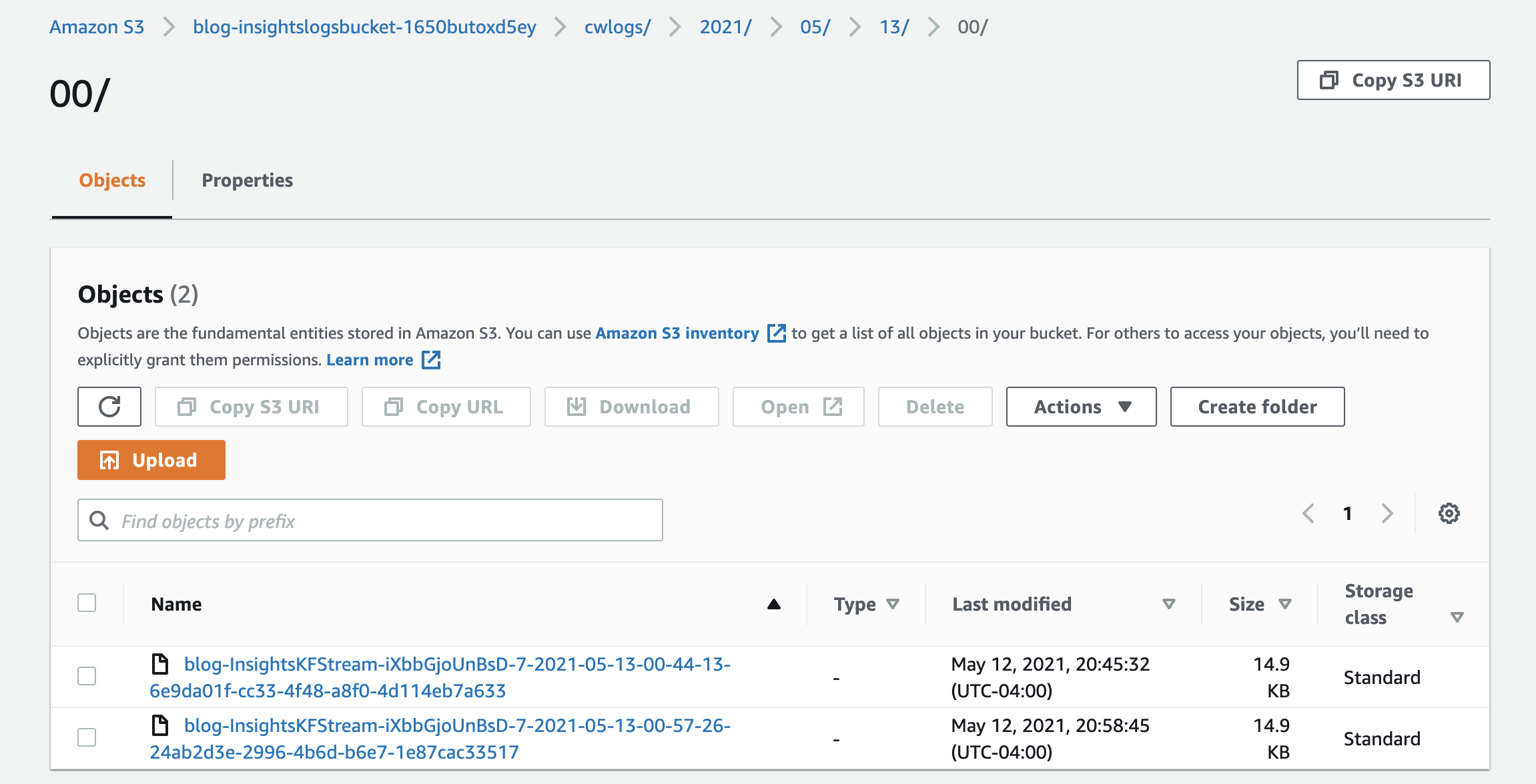
  1. On the Amazon S3 console, confirm the subfolders weather_hudi_cow and weather_hudi_mor are in athena-hudi-bucket.
  1. Navigate to the weather_hudi_cow subfolder to see the Apache Hudi dataset that is partitioned using the date key—one for each date in our dataset.
  2. On the Athena console, create a hudi_athena_test database using following command:
    create database hudi_athena_test;

You use this database to create all your tables.

  1. Create an Athena table using the athena_weather_hudi_cow.sql script:
    CREATE EXTERNAL TABLE weather_partition_cow(
      `_hoodie_commit_time` string,
      `_hoodie_commit_seqno` string,
      `_hoodie_record_key` string,
      `_hoodie_partition_path` string,
      `_hoodie_file_name` string,
      `city_id` string,
      `timestamp` string,
      `relative_humidity` decimal(3,1),
      `temperature` decimal(3,1),
      `absolute_humidity` decimal(5,4)
      )
      PARTITIONED BY ( 
      `date` string)
    ROW FORMAT SERDE
      'org.apache.hadoop.hive.ql.io.parquet.serde.ParquetHiveSerDe'
    STORED AS INPUTFORMAT
      'org.apache.hudi.hadoop.HoodieParquetInputFormat'
    OUTPUTFORMAT
      'org.apache.hadoop.hive.ql.io.parquet.MapredParquetOutputFormat'
    LOCATION
      's3://athena-hudi-bucket/hudi_weather/weather_hudi_cow'
    

Replace the S3 bucket path in the preceding code with your S3 bucket (Hudi table path) in LOCATION.

  1. Add partitions to the table by running the following query from the athena_weather_judi_cow.sql script on the Athena console:
    ALTER TABLE weather_partition_cow ADD
    PARTITION (date = '2020-10-01') LOCATION 's3://athena-hudi-bucket/hudi_weather/weather_hudi_cow/2020-10-01/'
    PARTITION (date = '2020-10-02') LOCATION 's3://athena-hudi-bucket/hudi_weather/weather_hudi_cow/2020-10-02/'
    PARTITION (date = '2020-10-03') LOCATION 's3://athena-hudi-bucket/hudi_weather/weather_hudi_cow/2020-10-03/'
    PARTITION (date = '2020-10-04') LOCATION 's3://athena-hudi-bucket/hudi_weather/weather_hudi_cow/2020-10-04/';

Replace the S3 bucket path in the preceding code with your S3 bucket (Hudi table path) in LOCATION.

  1. Confirm the total number of records in the Apache Hudi dataset with the following query:
    SELECT count(*) FROM "hudi_athena_test"."weather_partition_cow";

It should return a single row with a count of 1,000.

Now let’s check the record that we want to update.

  1. Run the following query on the Athena console:
    SELECT * FROM "hudi_athena_test"."weather_partition_cow"
    where city_id ='1'
    and date ='2020-10-04'
    and timestamp = '2020-10-04T07:19:12Z';

The output should look like the following screenshot. Note the value of relative_humidity and temperature.

  1. Return to the Amazon EMR primary node and run the following code in the data_insertion_cow_delta_script script on the spark-shell prompt to update the data:
    import org.apache.spark.sql.SaveMode
    import org.apache.spark.sql.functions._
    import org.apache.hudi.DataSourceWriteOptions
    import org.apache.hudi.config.HoodieWriteConfig
    import org.apache.hudi.hive.MultiPartKeysValueExtractor
    
    //Set up various input values as variables
    val inputDataPath = "s3://weather-raw-bucket/delta_parquet/"
    val hudiTableName = "weather_hudi_cow"
    val hudiTablePath = "s3://athena-hudi-bucket/hudi_weather/" + hudiTableName
    
    // Set up our Hudi Data Source Options
    val hudiOptions = Map[String,String](
        DataSourceWriteOptions.RECORDKEY_FIELD_OPT_KEY -> "city_id",
    	DataSourceWriteOptions.RECORDKEY_FIELD_OPT_KEY -> "timestamp",
        DataSourceWriteOptions.PARTITIONPATH_FIELD_OPT_KEY -> "date", 
        HoodieWriteConfig.TABLE_NAME -> hudiTableName, 
        DataSourceWriteOptions.OPERATION_OPT_KEY ->
            DataSourceWriteOptions.INSERT_OPERATION_OPT_VAL, 
        DataSourceWriteOptions.PRECOMBINE_FIELD_OPT_KEY -> "timestamp", 
        DataSourceWriteOptions.HIVE_SYNC_ENABLED_OPT_KEY -> "true", 
        DataSourceWriteOptions.HIVE_TABLE_OPT_KEY -> hudiTableName, 
        DataSourceWriteOptions.HIVE_PARTITION_FIELDS_OPT_KEY -> "date", 
        DataSourceWriteOptions.HIVE_PARTITION_EXTRACTOR_CLASS_OPT_KEY ->
            classOf[MultiPartKeysValueExtractor].getName)
    
    // Read data from S3 and create a DataFrame with Partition and Record Key
    val inputDF = spark.read.format("parquet").load(inputDataPath)
    
    // Write data into the Hudi dataset
    inputDF.write.format("org.apache.hudi").options(hudiOptions).mode(SaveMode.Append).save(hudiTablePath)
    

Replace the S3 bucket path for inputDataPath and hudiTablePath in the preceding code with your S3 bucket.

  1. Run the following query on the Athena console to confirm no change occurred to the total number of records:
SELECT count(*) FROM "hudi_athena_test"."weather_partition_cow";

The following screenshot shows our query results.

  1. Run the following query again on the Athena console to check for the update:
SELECT * FROM "hudi_athena_test"."weather_partition_cow"
where city_id ='1'
and date ='2020-10-04'
and timestamp = '2020-10-04T07:19:12Z'

The relative_humidity and temperature values for the relevant record are updated.

  1. Repeat similar steps for the MoR table.

Clean up the resources

You must clean up the resources you created earlier to avoid ongoing charges.

  1. On the AWS CloudFormation console, delete the stack you launched.
  2. On the Amazon S3 console, empty the buckets weather-raw-bucket and athena-hudi-bucket and delete the buckets.

Conclusion

As you have learned in this post, we used Apache Hudi support in Amazon EMR to develop a data pipeline to simplify incremental data management use cases that require record-level insert and update operations. We used Athena to read the read-optimized view of an Apache Hudi dataset in an S3 data lake.


About the Authors

Dhiraj Thakur is a Solutions Architect with Amazon Web Services. He works with AWS customers and partners to provide guidance on enterprise cloud adoption, migration and strategy. He is passionate about technology and enjoys building and experimenting in Analytics and AI/ML space.


Sameer Goel is a Solutions Architect in The Netherlands, who drives customer success by building prototypes on cutting-edge initiatives. Prior to joining AWS, Sameer graduated with a master’s degree from NEU Boston, with a Data Science concentration. He enjoys building and experimenting with creative projects and applications.


Imtiaz (Taz) Sayed is the WW Tech Master for Analytics at AWS. He enjoys engaging with the community on all things data and analytics.


How Jobcase is using Amazon Redshift ML to recommend job search content at scale

Post Syndicated from Clay Martin original https://aws.amazon.com/blogs/big-data/how-jobcase-is-using-amazon-redshift-ml-to-recommend-job-search-content-at-scale/

This post is co-written with Clay Martin and Ajay Joshi from Jobcase as the lead authors.

Jobcase is an online community dedicated to empowering and advocating for the world’s workers. We’re the third-largest destination for job search in the United States, and connect millions of Jobcasers to relevant job opportunities, companies, and other resources on a daily basis. Recommendation is central to everything we do.

In this post, Jobcase data scientists discuss how Amazon Redshift ML helped us generate billions of job search recommendations in record time and with improved relevance.

The challenge: Scaling job recommendations

At Jobcase, we have used Amazon Redshift as our primary data warehouse for 8 years. Over the years, we built up a significant amount of historical job seeker and job content interaction data, which is stored in highly optimized compressed tables.

Our recommender system applies machine learning (ML) models to these big datasets, which poses a familiar problem: the data and ML models aren’t colocated on the same compute clusters, which involves moving large amounts of data across networks. In many cases, at batch inference time, data must be shuttled out of—and eventually brought back into—a data warehouse, which can be a time-consuming, expensive, and sometimes error-prone process. This also requires data engineering resources to set up data pipelines, and often becomes a bottleneck for data scientists to perform quick experimentation and drive business value. Until now, this data/model colocation issue has proven to be a big obstacle to applying ML to batch recommendation at scale.

How Amazon Redshift ML helped solve this challenge

Amazon Redshift ML, powered by Amazon SageMaker Autopilot, makes it easy for data analysts and database developers to create, train, and apply ML models using familiar SQL commands in Amazon Redshift data warehouses.

Amazon Redshift ML has proven to be a great solution to some of these problems at Jobcase. With Amazon Redshift ML’s in-database local inference capability, we now perform model inference on billions of records in a matter of minutes, directly in our Amazon Redshift data warehouse. In this post, we talk about our journey to Amazon Redshift ML, our previous attempts to use ML for recommendations, and where we go from here.

What we’re trying to solve

Job search is a unique and challenging domain for recommender system design and implementation. There are extraordinary variables to consider. For instance, many job openings only last for days or weeks, and they must be within a reasonable commute for job seekers. Some jobs require skills that only a subset of our members possess. These constraints don’t necessarily apply to, say, movie recommendations. On the other hand, job preferences are relatively stable; if a member is interested in truck driver jobs on Monday, there’s a good chance they’re still interested on Tuesday.

The Jobcase recommender system is responsible for generating job search content for over 10 million active Jobcasers per day. On average, every day we have about 20–30 million unique job listings in the eligible pool for recommendations. The system runs overnight and generates predictions in batch mode, and is expected to be completed by early morning hours. These recommendations are used throughout the day to engage with Jobcase members through various communication channels like email, SMS, and push notifications.

Our recommendation system

Each communication channel has its own peculiarities and deliverability constraints. To handle these constraints, our recommender system is broken into multiple steps and phases, where the final step is used to fine-tune the model for a particular channel. All of this multi-channel job seeker interaction data resides in our Amazon Redshift cluster.

In phase one, we apply unsupervised learning techniques to reduce the candidate set of items per member. We calculate item-item similarity scores from members’ engagement histories, and use these scores to generate the N most similar items per user. This collaborative filtering phase poses an important design trade-off: filter out too many relevant candidate items, and member engagement drops; filter out too few, and downstream inference remains computationally infeasible.

The second phase is a channel-specific supervised learning phase. It uses the similarity score from the first phase along with other predicted metrics as features and attributes, and tries to directly predict member engagement for that channel. In this example, let’s assume email is the channel and member engagement is captured by the dependent variable email click-through rate (CTR) = email clicks/email sends.

Here we also include job seeker features, such as educational attainment, commute preferences, location, and so on, as well as item or job content features, such as channel-specific historical macro or local engagement rates. Generating predictions for over 10 million job seekers paired to 200–300 items per member requires 2–3 billion predictions for just one channel.

Simplifying ML from within Amazon Redshift without any data movement

Until now, our data/model colocation problem has been challenging to solve from a cost and performance perspective. This is where Amazon Redshift ML has been instrumental in significantly improving the recommender system by enabling billions of non-linear model predictions in just a few minutes.

Before Amazon Redshift ML, we needed to write custom data pipelines to get data out of the data warehouse to Amazon Simple Storage Service (Amazon S3), then to ML inference instances, and finally pipe predictions back into the data warehouse for consumption. This added additional time delays and cost. Historically, it has been a challenge to improve this phase, and we had to rely on relatively simple linear models, optimized via A/B testing and hard-coded into SQL statements.

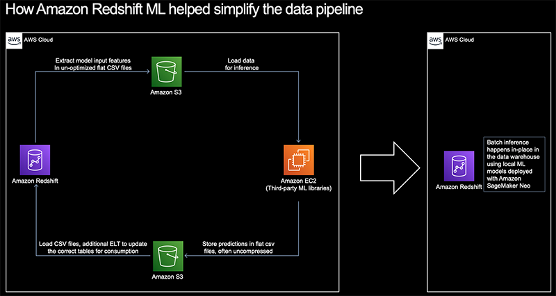
With Amazon Redshift ML, we were able to bring cutting-edge model classes with in-database local inference capabilities directly into our data warehouse. Therefore, the expressive power of the models that we could fit vastly increased. The following architecture diagram shows how we simplified our data pipeline with Amazon Redshift ML.

Our success story with Amazon Redshift ML

We have previously attempted to move one or both phases of our system out of Amazon Redshift. To improve our collaborative filtering phase, we tried using open-source libraries on Amazon Elastic Compute Cloud (Amazon EC2) instances that implement matrix factorization algorithms and natural language processing (NLP) inspired techniques such as Global Vectors (GloVe), which are distributed word representations. None of these solutions generated enough improvement in terms of member engagement to justify the increased data pipeline complexity, operational time delays, and operational expense. Pipelines to improve supervised user-item scoring had similar difficulties.

When Amazon Redshift ML was released in preview mode December 2020, we spun up a small Amazon Redshift cluster to test its capabilities against our use cases. We were immediately struck by the fact that Amazon Redshift ML makes fitting an XGBoost model or feed-forward neural network as easy as writing a SQL query. When Amazon Redshift ML became GA at the end of May 2021, we set it up in production within a day, and deployed a production model within a week. The following is a sample model that we trained and predicted with Amazon Redshift ML.

The following is the training code:

CREATE MODEL
f_ml_predict_email_content1_ctr
FROM (SELECT * FROM
Email_content1_click_history)
TARGET is_click
FUNCTION f_ml_predict_email_content1_ctr
PROBLEM_TYPE REGRESSION
OBJECTIVE 'MSE';

The following is the prediction code:

UPDATE email_content1_new_data
SET ctr_score = 
f_ml_predict_email_content1_ctr(
 feature1
,feature2,
 . . .
,feature_n)

Now we have several models in production, each performing billions of predictions in Amazon Redshift. The following are some of the key benefits we realized with Amazon Redshift ML:

  • Running model predictions at scale, performing billions of predictions in minutes, which we couldn’t achieve before implementing Amazon Redshift ML
  • Significant reduction in the model development cycle by eliminating the data pipelines
  • Significant reduction in model testing cycles by testing bigger cohort sizes, which helped reach our desired statistical significance quickly
  • Reduced cost by using Amazon Redshift ML’s local in-database inference capability, which saved cost on external ML frameworks and compute cost
  • 5–10% improvement in member engagement rates across several different email template types, resulting in increased revenue

Conclusion

In this post, we described how Amazon Redshift ML helped Jobcase effectively match millions of jobs to over 10 million active Jobcase members on a daily basis.

If you’re an Amazon Redshift user, Amazon Redshift ML provides an immediate and significant value add, with local in-database inference at no additional cost. It gives data scientists the ability to experiment quickly without data engineering dependencies. Amazon Redshift ML currently supports regression and classification model types, but is still able to achieve a great balance between speed, accuracy, complexity, and cost.


About Authors

Clay Martin is a Data Scientist at Jobcase Inc. He designs recommender systems to connect Jobcase members with the most relevant job content.


Ajay Joshi is Senior Software Engineer at Jobcase Inc. Ajay supports the data analytics and machine learning infrastructure at Jobcase and helps them design and maintain data warehouses powered by Amazon Redshift, Amazon SageMaker, and other AWS services.


Manash Deb is a Senior Analytics Specialist Solutions Architect at AWS. He has worked on building end-to-end data-driven solutions in different database and data warehousing technologies for over 15 years. He loves to learn new technologies and solving, automating, and simplifying customer problems with easy-to-use cloud data solutions on AWS.


Debu Panda, a Principal Product Manager at AWS, is an industry leader in analytics, application platform, and database technologies, and has more than 25 years of experience in the IT world.

Query Snowflake using Athena Federated Query and join with data in your Amazon S3 data lake

Post Syndicated from Navnit Shukla original https://aws.amazon.com/blogs/big-data/query-snowflake-using-athena-federated-query-and-join-with-data-in-your-amazon-s3-data-lake/

If you use data lakes in Amazon Simple Storage Service (Amazon S3) and use Snowflake as your data warehouse solution, you may need to join your data in your data lake with Snowflake. For example, you may want to build a dashboard by joining historical data in your Amazon S3 data lake and the latest data in your Snowflake data warehouse or create consolidated reporting.

In such use cases, Amazon Athena Federated Query allows you to seamlessly access the data from Snowflake without building ETL pipelines to copy or unload the data to the S3 data lake or Snowflake. This removes the overhead of creating additional extract, transform, and load (ETL) processes and shortens the development cycle.

In this post, we will walk you through a step-by-step configuration to set up Athena Federated Query using AWS Lambda to access data in a Snowflake data warehouse.

For this post, we are using the Snowflake connector for Amazon Athena developed by Trianz.

Let’s start with discussing the solution and then detailing the steps involved.

Solution overview

Data Federation refers to the capability to query data in another data store using a single interface (Amazon Athena). The following diagram depicts how a single Amazon Athena federated query uses Lambda to query the underlying data source and parallelizes execution across many workers.

Athena is an interactive query service that makes it easy to analyze data in Amazon S3 using standard SQL. If you have data in sources other than Amazon S3, you can use Athena Federated Query to query the data in place or build pipelines to extract data from multiple data sources and store them in Amazon S3. With Athena Federated Query, you can run SQL queries across data stored in relational, non-relational, object, and custom data sources.

When a federated query is run, Athena identifies the parts of the query that should be routed to the data source connector and executes them with Lambda. The data source connector makes the connection to the source, runs the query, and returns the results to Athena. If the data doesn’t fit into Lambda RAM runtime memory, it spills the data to Amazon S3 and is later accessed by Athena.

Athena uses data source connectors which internally use Lambda to run federated queries. Data source connectors are pre-built and can be deployed from the Athena console or from the Serverless Application Repository. Based on the user submitting the query, connectors can provide or restrict access to specific data elements.

To implement this solution, we complete the following steps:

  1. Create a secret for the Snowflake instance using AWS Secrets Manager.
  2. Create an S3 bucket and subfolder for Lambda to use.
  3. Configure Athena federation with the Snowflake instance.
  4. Run federated queries with Athena.

Prerequisites

Before getting started, make sure you have a Snowflake data warehouse up and running.

Create a secret for the Snowflake instance

Our first step is to create a secret for the Snowflake instance with a username and password using Secrets Manager.

  1. On the Secrets Manager console, choose Secrets.
  2. Choose Store a new secret.
  3. Select Other types of secrets.
  4. Enter the credentials as key-value pairs (username, password) for your Snowflake instance.
  5. For Secret name, enter a name for your secret. Use the prefix snowflake so it’s easy to find.

  1. Leave the remaining fields at their defaults and choose Next.
  2. Complete your secret creation.

Create an S3 bucket for Lambda

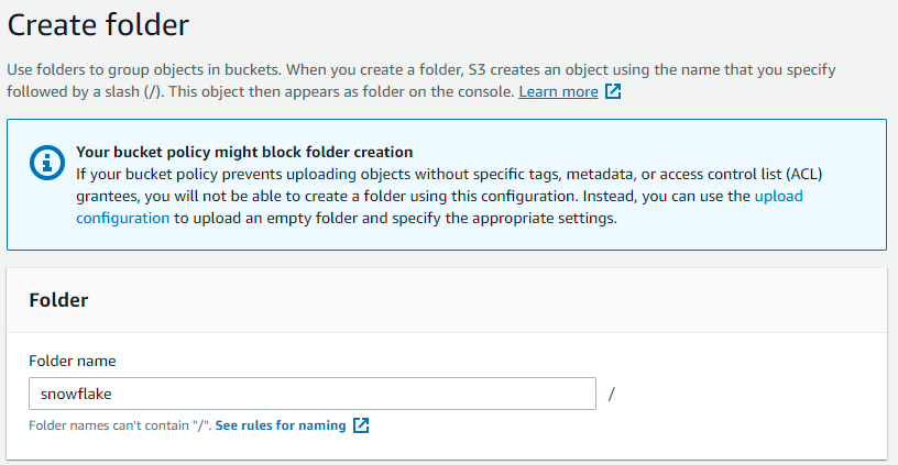
On the Amazon S3 console, create a new S3 bucket and subfolder for Lambda to use. For this post, we use athena-accelerator/snowflake.

Configure Athena federation with the Snowflake instance

To configure Athena data source connector for Snowflake with your Snowflake instance, complete the following steps:

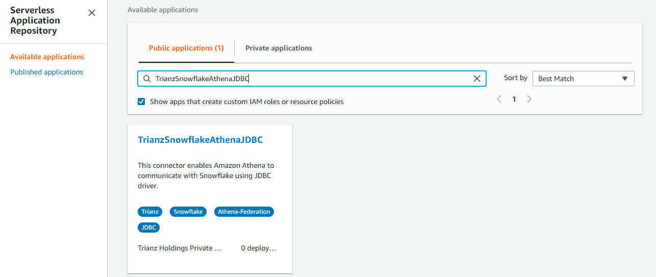
  1. On the AWS Serverless Application Repository console, choose Available applications.
  2. In the search field, enter TrianzSnowflakeAthenaJDBC.

  1. For Application name, enter TrianzSnowflakeAthenaJDBC.
  2. For SecretNamePrefix, enter trianz-snowflake-athena.
  3. For SpillBucket, enter Athena-accelerator/snowflake.
  4. For JDBCConnectorConfig, use the format snowflake://jdbc:snowflake://{snowflake_instance_url}/?warehouse={warehousename}&db={databasename}&schema={schemaname}&${secretname}

For example, we enter snowflake://jdbc:snowflake://trianz.snowflakecomputing.com/?warehouse=ATHENA_WH&db=ATHENA_DEV&schema=ATHENA&${trianz-snowflake-athena}DisableSpillEncyption – False

  1. For LambdaFunctionName, enter trsnowflake.
  2. For SecurityGroupID, enter the security group ID where the Snowflake instance is deployed.

Make sure to apply valid inbound and outbound rules based on your connection.

  1. For SpillPrefix, create a folder under the S3 bucket you created and specify the name (for example, athena-spill).
  2. For Subnetids, use the subnets where the Snowflake instance is running with comma separation.

Make sure the subnet is in a VPC and has NAT gateway and internet gateway attached.

  1. Select the I acknowledge check box.
  2. Choose Deploy.

Make sure that the AWS Identity and Access Management (IAM) roles have permissions to access AWS Serverless Application Repository, AWS CloudFormation, Amazon S3, Amazon CloudWatch, AWS CloudTrail, Secrets Manager, Lambda, and Athena. For more information, see Example IAM Permissions Policies to Allow Athena Federated Query.

Run federated queries with Athena

Before running your federated query, be sure that you have selected Athena engine version 2. The current Athena engine version for any workgroup can be found in the Athena console page.

Run your federated queries using lambda:trsnowflake to run against tables in the Snowflake database. This is the name of lambda function which we have created in step 7 of previous section of this blog.

lambda:trsnowflake is a reference data source connector Lambda function using the format lambda:MyLambdaFunctionName. For more information, see Writing Federated Queries.

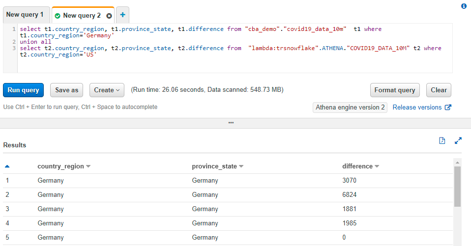
The following screenshot is a unionall query example of data in Amazon S3 with a table in the AWS Glue Data Catalog and a table in Snowflake.

Key performance best practices

If you’re considering Athena Federated Query with Snowflake, we recommend the following best practices:

  • Athena Federated query works great for queries with predicate filtering because the predicates are pushed down to the Snowflake database. Use filter and limited-range scans in your queries to avoid full table scans.
  • If your SQL query requires returning a large volume of data from Snowflake to Athena (which could lead to query timeouts or slow performance), you may consider copying data from Snowflake to your S3 data lake.
  • The Snowflake schema, which is an extension of the star schema, is used as a data model in Snowflake. In the Snowflake schema model, unload your large fact tables into your S3 data lake and leave the dimension tables in Snowflake. If large dimension tables are contributing to slow performance or query timeouts, unload those tables to your S3 data lake.
  • When you run federated queries, Athena spins up multiple Lambda functions, which causes a spike in database connections. It’s important to monitor the Snowflake database WLM queue slots to ensure there is no queuing. Additionally, you can use concurrency scaling on your Snowflake database cluster to benefit from concurrent connections to queue up.

Conclusion

In this post, you learned how to configure and use Athena federated with Snowflake using Lambda. With Athena Federated query user can leverage all of their data to produce analytics, derive business value without building ETL pipelines to bring data from different datastore such as Snowflake to Data Lake.

You can use the best practice considerations outlined in the post to help minimize the data transferred from Snowflake for better performance. When queries are well written for federation, the performance penalties are negligible.

For more information, see the Athena User Guide and Using Amazon Athena Federated Query.


About the Author

Navnit Shukla is AWS Specialist Solution Architect in Analytics. He is passionate about helping customers uncover insights from their data. He has been building solutions to help organizations make data-driven decisions.

Data Engineers of Netflix — Interview with Kevin Wylie

Post Syndicated from Netflix Technology Blog original https://netflixtechblog.com/data-engineers-of-netflix-interview-with-kevin-wylie-7fb9113a01ea

Data Engineers of Netflix — Interview with Kevin Wylie

This post is part of our “Data Engineers of Netflix” series, where our very own data engineers talk about their journeys to Data Engineering @ Netflix.

Kevin Wylie is a Data Engineer on the Content Data Science and Engineering team. In this post, Kevin talks about his extensive experience in content analytics at Netflix since joining more than 10 years ago.

Kevin grew up in the Washington, DC area, and received his undergraduate degree in Mathematics from Virginia Tech. Before joining Netflix, he worked at MySpace, helping implement page categorization, pathing analysis, sessionization, and more. In his free time he enjoys gardening and playing sports with his 4 kids.

His favorite TV shows: Ozark, Breaking Bad, Black Mirror, Barry, and Chernobyl

Since I joined Netflix back in 2011, my favorite project has been designing and building the first version of our entertainment knowledge graph. The knowledge graph enabled us to better understand the trends of movies, TV shows, talent, and books. Building the knowledge graph offered many interesting technical challenges such as entity resolution (e.g., are these two movie names in different languages really the same?), and distributed graph algorithms in Spark. After we launched the product, analysts and scientists began surfacing new insights that were previously hidden behind difficult-to-use data. The combination of overcoming technical hurdles and creating new opportunities for analysis was rewarding.

Kevin, what drew you to data engineering?

I stumbled into data engineering rather than making an intentional career move into the field. I started my career as an application developer with basic familiarity with SQL. I was later hired into my first purely data gig where I was able to deepen my knowledge of big data. After that, I joined MySpace back at its peak as a data engineer and got my first taste of data warehousing at internet-scale.

What keeps me engaged and enjoying data engineering is giving super-suits and adrenaline shots to analytics engineers and data scientists.

When I make something complex seem simple, or create a clean environment for my stakeholders to explore, research and test, I empower them to do more impactful business-facing work. I like that data engineering isn’t in the limelight, but instead can help create economies of scale for downstream analytics professionals.

What drew you to Netflix?

My wife came across the Netflix job posting in her effort to keep us in Los Angeles near her twin sister’s family. As a big data engineer, I found that there was an enormous amount of opportunity in the Bay Area, but opportunities were more limited in LA where we were based at the time. So the chance to work at Netflix was exciting because it allowed me to live closer to family, but also provided the kind of data scale that was most common for Bay Area companies.

The company was intriguing to begin with, but I knew nothing of the talent, culture, or leadership’s vision. I had been a happy subscriber of Netflix’s DVD-rental program (no late fees!) for years.

After interviewing, it became clear to me that this company culture was different than any I had experienced.

I was especially intrigued by the trust they put in each employee. Speaking with fellow employees allowed me to get a sense for the kinds of people Netflix hires. The interview panel’s humility, curiosity and business acumen was quite impressive and inspired me to join them.

I was also excited by the prospect of doing analytics on movies and TV shows, which was something I enjoyed exploring outside of work. It seemed fortuitous that the area of analytics that I’d be working in would align so well with my hobbies and interests!

Kevin, you’ve been at Netflix for over 10 years now, which is pretty incredible. Over the course of your time here, how has your role evolved?

When I joined Netflix back in 2011, our content analytics team was just 3 people. We had a small office in Los Angeles focused on content, and significantly more employees at the headquarters in Los Gatos. The company was primarily thought of as a tech company.

At the time, the data engineering team mainly used a data warehouse ETL tool called Ab Initio, and an MPP (Massively Parallel Processing) database for warehousing. Both were appliances located in our own data center. Hadoop was being lightly tested, but only in a few high-scale areas.

Fast forward 10 years, and Netflix is now the leading streaming entertainment service — serving members in over 190 countries. In the data engineering space, very little of the same technology remains. Our data centers are retired, Hadoop has been replaced by Spark, Ab Initio and our MPP database no longer fits our big data ecosystem.

In addition to the company and tech shifting, my role has evolved quite a bit as our company has grown. When we were a smaller company, the ability to span multiple functions was valued for agility and speed of delivery. The sooner we could ingest new data and create dashboards and reports for non-technical users to explore and analyze, the sooner we could deliver results. But now, we have a much more mature business, and many more analytics stakeholders that we serve.

For a few years, I was in a management role, leading a great team of people with diverse backgrounds and skill sets. However, I missed creating data products with my own hands so I wanted to step back into a hands-on engineering role. My boss was gracious enough to let me make this change and focus on impacting the business as an individual contributor.

As I think about my future at Netflix, what motivates me is largely the same as what I’ve always been passionate about. I want to make the lives of data consumers easier and to enable them to be more impactful. As the company scales and as we continue to invest in storytelling, the opportunity grows for me to influence these decisions through better access to information and insights. The biggest impact I can make as a data engineer is creating economies of scale by producing data products that will serve a diverse set of use cases and stakeholders.

If I can build beautifully simple data products for analytics engineers, data scientists, and analysts, we can all get better at Netflix’s goal: entertaining the world.

Learning more

Interested in learning more about data roles at Netflix? You’re in the right place! Keep an eye out for our open roles in Data Science and Engineering by visiting our jobs site here. Our culture is key to our impact and growth: read about it here. To learn more about our Data Engineers, check out our chats with Dhevi Rajendran and Samuel Setegne.


Data Engineers of Netflix — Interview with Kevin Wylie was originally published in Netflix TechBlog on Medium, where people are continuing the conversation by highlighting and responding to this story.

Build a serverless event-driven workflow with AWS Glue and Amazon EventBridge

Post Syndicated from Noritaka Sekiyama original https://aws.amazon.com/blogs/big-data/build-a-serverless-event-driven-workflow-with-aws-glue-and-amazon-eventbridge/

Customers are adopting event-driven-architectures to improve the agility and resiliency of their applications. As a result, data engineers are increasingly looking for simple-to-use yet powerful and feature-rich data processing tools to build pipelines that enrich data, move data in and out of their data lake and data warehouse, and analyze data. AWS Glue is a serverless data integration service that makes it easy to discover, prepare, and combine data for analytics, machine learning, and application development. AWS Glue provides all the capabilities needed for data integration so that you can start analyzing your data and putting it to use in minutes instead of months.

Data integration jobs have varying degrees of priority and time sensitivity. For example, you can use batch processing to process weekly sales data but in some cases, data needs to be processed immediately. Fraud detection applications, for example, require near-real-time processing of security logs. Or if a partner uploads product information to your Amazon Simple Storage Service (Amazon S3) bucket, it needs to be processed right away to ensure that your website has the latest product information.

This post discusses how to configure AWS Glue workflows to run based on real-time events. You no longer need to set schedules or build complex solutions to trigger jobs based on events; AWS Glue event-driven workflows manage it all for you.

Get started with AWS Glue event-driven workflows

As a business requirement, most companies need to hydrate their data lake and data warehouse with data in near-real time. They run their pipelines on a schedule (hourly, daily, or even weekly) or trigger the pipeline through an external system. It’s difficult to predict the frequency at which upstream systems generate data, which makes it difficult to plan and schedule ETL pipelines to run efficiently. Scheduling ETL pipelines to run too frequently can be expensive, whereas scheduling pipelines to run infrequently can lead to making decisions based on stale data. Similarly, triggering pipelines from an external process can increase complexity, cost, and job startup time.

AWS Glue now supports event-driven workflows, a capability that lets developers start AWS Glue workflows based on events delivered by Amazon EventBridge. With this new feature, you can trigger a data integration workflow from any events from AWS services, software as a service (SaaS) providers, and any custom applications. For example, you can react to an S3 event generated when new buckets are created and when new files are uploaded to a specific S3 location. In addition, if your environment generates many events, AWS Glue allows you to batch them either by time duration or by the number of events. Event-driven workflows make it easy to start an AWS Glue workflow based on real-time events.

To get started, you simply create a new AWS Glue trigger of type EVENT and place it as the first trigger in your workflow. You can optionally specify a batching condition. Without event batching, the AWS Glue workflow is triggered every time an EventBridge rule matches which may result in multiple concurrent workflow runs. In some environments, starting many concurrent workflow runs could lead to throttling, reaching service quota limits, and potential cost overruns. This can also result in workflow execution failures in case the concurrency limit specified on the workflow and the jobs within the workflow do not match. Event batching allows you to configure the number of events to buffer or the maximum elapsed time before firing the particular trigger. Once the batching condition is met, a workflow run is started. For example, you can trigger your workflow when 100 files are uploaded in S3 or 5 minutes after the first upload. We recommend configuring event batching to avoid too many concurrent workflow runs, and optimize resource usage and cost.

Overview of the solution

In this post, we walk through a solution to set up an AWS Glue workflow that listens to S3 PutObject data events captured by AWS CloudTrail. This workflow is configured to run when five new files are added or the batching window time of 900 seconds expires after first file is added. The following diagram illustrates the architecture.

The steps in this solution are as follows:

  1. Create an AWS Glue workflow with a starting trigger of EVENT type and configure the batch size on the trigger to be five and batch window to be 900 seconds.
  2. Configure Amazon S3 to log data events, such as PutObject API calls to CloudTrail.
  3. Create a rule in EventBridge to forward the PutObject API events to AWS Glue when they are emitted by CloudTrail.
  4. Add an AWS Glue event-driven workflow as a target to the EventBridge rule.
  5. To start the workflow, upload files to the S3 bucket. Remember you need to have at least five files before the workflow is triggered.

Deploy the solution with AWS CloudFormation

For a quick start of this solution, you can deploy the provided AWS CloudFormation stack. This creates all the required resources in your account.

The CloudFormation template generates the following resources:

  • S3 bucket – This is used to store data, CloudTrail logs, job scripts, and any temporary files generated during the AWS Glue ETL job run.
  • CloudTrail trail with S3 data events enabled – This enables EventBridge to receive PutObject API call data on specific bucket.
  • AWS Glue workflow – A data processing pipeline that is comprised of a crawler, jobs, and triggers. This workflow converts uploaded data files into Apache Parquet format.
  • AWS Glue database – The AWS Glue Data Catalog database that is used to hold the tables created in this walkthrough.
  • AWS Glue table – The Data Catalog table representing the Parquet files being converted by the workflow.
  • AWS Lambda function – This is used as an AWS CloudFormation custom resource to copy job scripts from an AWS Glue-managed GitHub repository and an AWS Big Data blog S3 bucket to your S3 bucket.
  • IAM roles and policies – We use the following AWS Identity and Access Management (IAM) roles:
    • LambdaExecutionRole – Runs the Lambda function that has permission to upload the job scripts to the S3 bucket.
    • GlueServiceRole – Runs the AWS Glue job that has permission to download the script, read data from the source, and write data to the destination after conversion.
    • EventBridgeGlueExecutionRole – Has permissions to invoke the NotifyEvent API for an AWS Glue workflow.

To launch the CloudFormation stack, complete the following steps:

  1. Sign in to the AWS CloudFormation console.
  2. Choose Launch Stack:

  1. Choose Next.
  2. For S3BucketName, enter the unique name of your new S3 bucket.
  3. For WorkflowName, DatabaseName, and TableName, leave as the default.
  4. Choose Next.

  1. On the next page, choose Next.
  2. Review the details on the final page and select I acknowledge that AWS CloudFormation might create IAM resources.
  3. Choose Create.

It takes a few minutes for the stack creation to complete; you can follow the progress on the Events tab.

By default, the workflow runs whenever a single file is uploaded to the S3 bucket, resulting in a PutObject API call. In the next section, we configure the event batching to change this behavior.

Review the AWS Glue trigger and add event batching conditions

The CloudFormation template provisioned an AWS Glue workflow including a crawler, jobs, and triggers. The first trigger in the workflow is configured as an event-based trigger. Next, we update this trigger to batch five events or wait for 900 seconds after the first event before it starts the workflow.

Before we make any changes, let’s review the trigger on the AWS Glue console:

  1. On the AWS Glue console, under ETL, choose Triggers.
  2. Choose <Workflow-name>_pre_job_trigger.
  3. Choose Edit.

We can see the trigger’s type is set to EventBridge event, which means it’s an event-based trigger. Let’s change the event batching condition to run the workflow after five files are uploaded to Amazon S3.

  1. For Number of events, enter 5.
  2. For Time delay (sec), enter 900.
  3. Choose Next.

  1. On the next screen, under Choose jobs to trigger, leave as the default and choose Next.
  2. Choose Finish.

Review the EventBridge rule

The CloudFormation template created an EventBridge rule to forward S3 PutObject API events to AWS Glue. Let’s review the configuration of the EventBridge rule:

  1. On the EventBridge console, under Events, choose Rules.
  2. Choose s3_file_upload_trigger_rule-<CloudFormation-stack-name>.
  3. Review the information in the Event pattern section.

The event pattern shows that this rule is triggered when an S3 object is uploaded to s3://<bucket_name>/data/products_raw/. CloudTrail captures the PutObject API calls made and relays them as events to EventBridge.

  1. In the Targets section, you can verify that this EventBridge rule is configured with an AWS Glue workflow as a target.

Trigger the AWS Glue workflow by uploading files to Amazon S3

To test your workflow, we upload files to Amazon S3 using the AWS Command Line Interface (AWS CLI). If you don’t have the AWS CLI, see Installing, updating, and uninstalling the AWS CLI.

Let’s upload some small files to your S3 bucket.

  1. Run the following command to upload the first file to your S3 bucket:
$ echo '{"product_id": "00001", "product_name": "Television", "created_at": "2021-06-01"}' > product_00001.json
$ aws s3 cp product_00001.json s3://<bucket-name>/data/products_raw/
  1. Run the following command to upload the second file:
$ echo '{"product_id": "00002", "product_name": "USB charger", "created_at": "2021-06-02"}' > product_00002.json
$ aws s3 cp product_00002.json s3://<bucket-name>/data/products_raw/
  1. Run the following command to upload the third file:
$ echo '{"product_id": "00003", "product_name": "USB charger", "created_at": "2021-06-03"}' &gt; product_00003.json<br />
$ aws s3 cp product_00003.json s3://<bucket-name>/data/products_raw/
  1. Run the following command to upload the fourth file:
$ echo '{"product_id": "00004", "product_name": "USB charger", "created_at": "2021-06-04"}' &gt; product_00004.json<br />
$ aws s3 cp product_00004.json s3://<bucket-name>/data/products_raw/

These events didn’t trigger the workflow because it didn’t meet the batch condition of five events.

  1. Run the following command to upload the fifth file:
$ echo '{"product_id": "00005", "product_name": "USB charger", "created_at": "2021-06-05"}' > product_00005.json
$ aws s3 cp product_00005.json s3://<bucket-name>/data/products_raw/

Now the five JSON files have been uploaded to Amazon S3.

Verify the AWS Glue workflow is triggered successfully

Now the workflow should be triggered. Open the AWS Glue console to validate that your workflow is in the RUNNING state.

To view the run details, complete the following steps:

  1. On the History tab of the workflow, choose the current or most recent workflow run.
  2. Choose View run details.

When the workflow run status changes to Completed, let’s see the converted files in your S3 bucket.

  1. Switch to the Amazon S3 console, and navigate to your bucket.

You can see the Parquet files under s3://<bucket-name>/data/products/.

Congratulations! Your workflow ran successfully based on S3 events triggered by uploading files to your bucket. You can verify everything works as expected by running a query against the generated table using Amazon Athena.

Verify the metrics for the EventBridge rule

Optionally, you can use Amazon CloudWatch metrics to validate the events were sent to the AWS Glue workflow.

  1. On the EventBridge console, in the navigation pane, choose Rules.
  2. Select your EventBridge rule s3_file_upload_trigger_rule-<Workflow-name> and choose Metrics for the rule.

When the target workflow is invoked by the rule, the metrics Invocations and TriggeredRules are published.

The metric FailedInvocations is published if the EventBridge rule is unable to trigger the AWS Glue workflow. In that case, we recommend you check the following configurations:

  • Verify the IAM role provided to the EventBridge rule allows the glue:NotifyEvent permission on the AWS Glue workflow.
  • Verify the trust relationship on the IAM role provides the events.amazonaws.com service principal the ability to assume the role.
  • Verify the starting trigger on your target AWS Glue workflow is an event-based trigger.

Clean up

Now to the final step, cleaning up the resources. Delete the CloudFormation stack to remove any resources you created as part of this walkthrough.

Conclusion

AWS Glue event-driven workflows enable data engineers to easily build event driven ETL pipelines that respond in near-real time, delivering fresh data to business users. In this post, we demonstrated how to configure a rule in EventBridge to forward events to AWS Glue. We also saw how to create an event-based trigger that either immediately, or after a set number of events or period of time, starts a Glue ETL workflow. Migrating your existing AWS Glue workflows to make them event-driven is easy. This can be simply done by replacing the first trigger in the workflow to be of type EVENT and adding this workflow as a target to an EventBridge rule that captures events of your interest.

For more information about event-driven AWS Glue workflows, see Starting an AWS Glue Workflow with an Amazon EventBridge Event.


About the Authors

Noritaka Sekiyama is a Senior Big Data Architect on the AWS Glue and AWS Lake Formation team. In his spare time, he enjoys playing with his children. They are addicted to grabbing crayfish and worms in the park, and putting them in the same jar to observe what happens.


Karan Vishwanathan is a Software Development Engineer on the AWS Glue team. He enjoys working on distributed systems problems and playing golf.


Keerthi Chadalavada is a Software Development Engineer on the AWS Glue team. She is passionate about building fault tolerant and reliable distributed systems at scale.

Auto scaling Amazon Kinesis Data Streams using Amazon CloudWatch and AWS Lambda

Post Syndicated from Matthew Nolan original https://aws.amazon.com/blogs/big-data/auto-scaling-amazon-kinesis-data-streams-using-amazon-cloudwatch-and-aws-lambda/

This post is co-written with Noah Mundahl, Director of Public Cloud Engineering at United Health Group.

In this post, we cover a solution to add auto scaling to Amazon Kinesis Data Streams. Whether you have one stream or many streams, you often need to scale them up when traffic increases and scale them down when traffic decreases. Scaling your streams manually can create a lot of operational overhead. If you leave your streams overprovisioned, costs can increase. If you want the best of both worlds—increased throughput and reduced costs—then auto scaling is a great option. This was the case for United Health Group. Their Director of Public Cloud Engineering, Noah Mundahl, joins us later in this post to talk about how adding this auto scaling solution impacted their business.

Overview of solution

In this post, we showcase a lightweight serverless architecture that can auto scale one or many Kinesis data streams based on throughput. It uses Amazon CloudWatch, Amazon Simple Notification Service (Amazon SNS), and AWS Lambda. A single SNS topic and Lambda function process the scaling of any number of streams. Each stream requires one scale-up and one scale-down CloudWatch alarm. For an architecture that uses Application Auto Scaling, see Scale Amazon Kinesis Data Streams with AWS Application Auto Scaling.

The workflow is as follows:

  1. Metrics flow from the Kinesis data stream into CloudWatch (bytes/second, records/second).
  2. Two CloudWatch alarms, scale-up and scale-down, evaluate those metrics and decide when to scale.
  3. When one of these scaling alarms triggers, it sends a message to the scaling SNS topic.
  4. The scaling Lambda function processes the SNS message:
    1. The function scales the data stream up or down using UpdateShardCount:
      1. Scale-up events double the number of shards in the stream
      2. Scale-down events halve the number of shards in the stream
    2. The function updates the metric math on the scale-up and scale-down alarms to reflect the new shard count.

Implementation

The scaling alarms rely on CloudWatch alarm metric math to calculate a stream’s maximum usage factor. This usage factor is a percentage calculation from 0.00–1.00, with 1.00 meaning the stream is 100% utilized in either bytes per second or records per second. We use the usage factor for triggering scale-up and scale-down events. Our alarms use the following usage factor thresholds to trigger scaling events: >= 0.75 for scale-up and < 0.25 for scale-down. We use 5-minute data points (period) on all alarms because they’re more resistant to Kinesis traffic micro spikes.

Scale-up usage factor

The following screenshot shows the metric math on a scale-up alarm.

The scale-up max usage factor for a stream is calculated as follows:

s1 = Current shard count of the stream
m1 = Incoming Bytes Per Period, directly from CloudWatch metrics
m2 = Incoming Records Per Period, directly from CloudWatch metrics
e1 = Incoming Bytes Per Period with missing data points filled by zeroes
e2 = Incoming Records Per Period with missing data points filled by zeroes
e3 = Incoming Bytes Usage Factor 
   = Incoming Bytes Per Period / Max Bytes Per Period
   = e1/(1024*1024*60*$kinesis_period_mins*s1)
e4 = Incoming Records Usage Factor  
   = Incoming Records Per Period / Max Records Per Period 
   = e2/(1000*60*$kinesis_period_mins*s1) 
e6 = Max Usage Factor: Incoming Bytes or Incoming Records 
   = MAX([e3,e4])

Scale-down usage factor

We calculate the scale-down usage factor the same as the scale-up usage factor with some additional metric math to (optionally) take into account the iterator age of the stream to block scale-downs when stream processing is falling behind. This is useful if you’re using Lambda functions per shard, known as the Parallelization Factor, to process your streams. If you have a backlog of data, scaling down reduces the number of Lambda functions you need to process that backlog.

The following screenshot shows the metric math on a scale-down alarm.

The scale-down max usage factor for a stream is calculated as follows:

s1 = Current shard count of the stream
s2 = Iterator Age (in minutes) after which we begin blocking scale downs	
m1 = Incoming Bytes Per Period, directly from CloudWatch metrics
m2 = Incoming Records Per Period, directly from CloudWatch metrics
e1 = Incoming Bytes Per Period with missing data points filled by zeroes
e2 = Incoming Records Per Period with missing data points filled by zeroes
e3 = Incoming Bytes Usage Factor 
   = Incoming Bytes Per Period / Max Bytes Per Period
   = e1/(1024*1024*60*$kinesis_period_mins*s1)
e4 = Incoming Records Usage Factor  
   = Incoming Records Per Period / Max Records Per Period 
   = e2/(1000*60*$kinesis_period_mins*s1)
e5 = Iterator Age Adjusted Factor 
   = Scale Down Threshold * (Iterator Age Minutes / Iterator Age Minutes to Block Scale Down)
   = $kinesis_scale_down_threshold * ((FILL(m3,0)*1000/60)/s2)
e6 = Max Usage Factor: Incoming Bytes, Incoming Records, or Iterator Age Adjusted Factor
   = MAX([e3,e4,e5])

Deployment

You can deploy this solution via AWS CloudFormation. For more information, see the GitHub repo.

If you need to generate traffic on your streams for testing, consider using the Amazon Kinesis Data Generator. For more information, see Test Your Streaming Data Solution with the New Amazon Kinesis Data Generator.

Optum’s story

As the health services innovation arm of UnitedHealth Group, Optum has been on a multi-year journey towards advancing maturity and capabilities in the public cloud. Our multi-cloud strategy includes using many cloud-native services offered by AWS. The elasticity and self-healing features of the public cloud are among of its many strengths, and we use the automation provided natively by AWS through auto scaling capabilities. However, some services don’t natively provide those capabilities, such as Kinesis Data Streams. That doesn’t mean that we’re complacent and accept inelasticity.

Reducing operational toil

At the scale Optum operates at in the public cloud, monitoring for errors or latency related to our Kinesis data stream shard count and manually adjusting those values in response could become a significant source of toil for our public cloud platform engineering teams. Rather than engaging in that toil, we prefer to engineer automated solutions that respond much faster than humans and help us maintain performance, data resilience, and cost-efficiency.

Serving our mission through engineering

Optum is a large organization with thousands of software engineers. Our mission is to help people live healthier lives and help make the health system work better for everyone. To accomplish that mission, our public cloud platform engineers must act as force multipliers across the organization. With solutions such as this, we ensure that our engineers can focus on building and not on responding to needless alerts.

Conclusion

In this post, we presented a lightweight auto scaling solution for Kinesis Data Streams. Whether you have one stream or many streams, this solution can handle scaling for you. The benefits include less operational overhead, increased throughput, and reduced costs. Everything you need to get started is available on the Kinesis Auto Scaling GitHub repo.


About the authors

Matthew NolanMatthew Nolan is a Senior Cloud Application Architect at Amazon Web Services. He has over 20 years of industry experience and over 10 years of cloud experience. At AWS he helps customers rearchitect and reimagine their applications to take full advantage of the cloud. Matthew lives in New England and enjoys skiing, snowboarding, and hiking.


Paritosh Walvekar Paritosh Walvekar is a Cloud Application Architect with AWS Professional Services, where he helps customers build cloud native applications. He has a Master’s degree in Computer Science from University at Buffalo. In his free time, he enjoys watching movies and is learning to play the piano.


Noah Mundahl Noah Mundahl is Director of Public Cloud Engineering at United Health Group.

Data preparation using an Amazon RDS for MySQL database with AWS Glue DataBrew

Post Syndicated from Dhiraj Thakur original https://aws.amazon.com/blogs/big-data/data-preparation-using-an-amazon-rds-for-mysql-database-with-aws-glue-databrew/

With AWS Glue DataBrew, data analysts and data scientists can easily access and visually explore any amount of data across their organization directly from their Amazon Simple Storage Service (Amazon S3) data lake, Amazon Redshift data warehouse, or Amazon Aurora and Amazon Relational Database Service (Amazon RDS) databases. You can choose from over 250 built-in functions to merge, pivot, and transpose the data without writing code.

Now, with added support for JDBC-accessible databases, DataBrew also supports additional data stores, including PostgreSQL, MySQL, Oracle, and Microsoft SQL Server. In this post, we use DataBrew to clean data from an RDS database, store the cleaned data in an S3 data lake, and build a business intelligence (BI) report.

Use case overview

For our use case, we use three datasets:

  • A school dataset that contains school details like school ID and school name
  • A student dataset that contains student details like student ID, name, and age
  • A student study details dataset that contains student study time, health, country, and more

The following diagram shows the relation of these tables.

For our use case, this data is collected by a survey organization after an annual exam, and updates are made in Amazon RDS for MySQL using a Java script-based frontend application. We join the tables to create a single view and create aggregated data through a series of data preparation steps, and the business team uses the output data to create BI reports.

Solution overview

The following diagram illustrates our solution architecture. We use Amazon RDS to store data, DataBrew for data preparation, Amazon Athena for data analysis with standard SQL, and Amazon QuickSight for business reporting.

The workflow includes the following steps:
  1. Create a JDBC connection for RDS and a DataBrew project. DataBrew does the transformation to find the top performing students across all the schools considered for analysis.
  2. The DataBrew job writes the final output to our S3 output bucket.
  3. After the output data is written, we can create external tables on top of it with Athena create table statements and load partitions with MCSK REPAIR commands.
  4. Business users can use QuickSight for BI reporting, which fetches data through Athena. Data analysts can also use Athena to analyze the complete refreshed dataset.

Prerequisites

To complete this solution, you should have an AWS account.

Prelab setup

Before beginning this tutorial, make sure you have the required permissions to create the resources required as part of the solution.

For our use case, we use three mock datasets. You can download the DDL code and data files from GitHub.

  1. Create the RDS for MySQL instance to capture the student health data.
  2. Make sure you have set up the correct security group for Amazon RDS. For more information, see Setting Up a VPC to Connect to JDBC Data Stores.
  3. Create three tables: student_tbl, study_details_tbl, and school_tbl. You can use DDLsql to create the database objects.
  4. Upload the student.csv, study_details.csv, and school.csv files in their respective tables. You can use student.sql, study_details.sql, and school.sql to insert the data in the tables.

Create an Amazon RDS connection

To create your Amazon RDS connection, complete the following steps:

  1. On the DataBrew console, choose Datasets.
  2. On the Connections tab, choose Create connection.

  1. For Connection name, enter a name (for example, student_db-conn).
  2. For Connection type, select JDBC.
  3. For Database type, choose MySQL.

  1. Provide other parameters like RDS endpoint, port, database name, and database login credentials.

  1. In the Network options section, choose the VPC, subnet, and security group of your RDS instance.
  2. Choose Create connection.

Create your datasets

We have three tables in Amazon RDS: school_tbl, student_tbl, and study_details_tbl. To use these tables, we first need to create a dataset for each table.

To create the datasets, complete the following steps (we walk you through creating the school dataset):

  1. On the Datasets page of the DataBrew console, choose Connect new dataset.

  1. For Dataset name, enter school-dataset.
  2. Choose the connection you created (AwsGlueDatabrew-student-db-conn).
  3. For Table name, enter school_tbl.
  4. Choose Create dataset.

  1. Repeat these steps for the student_tbl and study_details_tbl tables, and name the new datasets student-dataset and study-detail-dataset, respectively.

All three datasets are available to use on the Datasets page.

Create a project using the datasets

To create your DataBrew project, complete the following steps:

  1. On the DataBrew console, choose Projects.
  2. Choose Create project.
  3. For Project Name, enter my-rds-proj.
  4. For Attached recipe, choose Create new recipe.

The recipe name is populated automatically.

  1. For Select a dataset, select My datasets.
  2. For Dataset name, select study-detail-dataset.

  1. For Role name, choose your AWS Identity and Access management (IAM) role to use with DataBrew.
  2. Choose Create project.

You can see a success message along with our RDS study_details_tbl table with 500 rows.

After the project is opened, a DataBrew interactive session is created. DataBrew retrieves sample data based on your sampling configuration selection.

Open an Amazon RDS project and build a transformation recipe

In a DataBrew interactive session, you can cleanse and normalize your data using over 250 built-in transforms. In this post, we use DataBrew to identify top performing students by performing a few transforms and finding students who got marks greater than or equal to 60 in the last annual exam.

First, we use DataBrew to join all three RDS tables. To do this, we perform the following steps:

  1. Navigate to the project you created.
  2. Choose Join.

  1. For Select dataset, choose student-dataset.
  2. Choose Next.

  1. For Select join type, select Left join.
  2. For Join keys, choose student_id for Table A and deselect student_id for Table B.
  3. Choose Finish.

Repeat the steps for school-dataset based on the school_id key.

  1. Choose MERGE to merge first_name and last_name.
  2. Enter a space as a separator.
  3. Choose Apply.

We now filter the rows based on marks value greater than or equal to 60 and add the condition as a recipe step.

  1. Choose FILTER.

  1. Provide the source column and filter condition and choose Apply.

The final data shows the top performing students’ data who had marks greater than or equal to 60.

Run the DataBrew recipe job on the full data

Now that we have built the recipe, we can create and run a DataBrew recipe job.

  1. On the project details page, choose Create job.
  2. For Job name¸ enter top-performer-student.

For this post, we use Parquet as the output format.

  1. For File type, choose PARQUET.
  2. For S3 location, enter the S3 path of the output folder.

  1. For Role name, choose an existing role or create a new one.
  2. Choose Create and run job.

  1. Navigate to the Jobs page and wait for the top-performer-student job to complete.

  1. Choose the Destination link to navigate to Amazon S3 to access the job output.

Run an Athena query

Let’s validate the aggregated table output in Athena by running a simple SELECT query. The following screenshot shows the output.

Create reports in QuickSight

Now let’s do our final step of the architecture, which is creating BI reports through QuickSight by connecting to the Athena aggregated table.

  1. On the QuickSight console, choose Athena as your data source.

  1. Choose the database and catalog you have in Athena.
  2. Select your table.
  3. Choose Select.

Now you can create a quick report to visualize your output, as shown in the following screenshot.

If QuickSight is using SPICE storage, you need to refresh the dataset in QuickSight after you receive notification about the completion of the data refresh. We recommend using SPICE storage to get better performance.

Clean up

Delete the following resources that might accrue cost over time:

  • The RDS instance
  • The recipe job top-performer-student
  • The job output stored in your S3 bucket
  • The IAM roles created as part of projects and jobs
  • The DataBrew project my-rds-proj and its associated recipe my-rds-proj-recipe
  • The DataBrew datasets

Conclusion

In this post, we saw how to create a JDBC connection for an RDS database. We learned how to use this connection to create a DataBrew dataset for each table, and how to reuse this connection multiple times. We also saw how we can bring data from Amazon RDS into DataBrew and seamlessly apply transformations and run recipe jobs that refresh transformed data for BI reporting.


About the Author

Dhiraj Thakur is a Solutions Architect with Amazon Web Services. He works with AWS customers and partners to provide guidance on enterprise cloud adoption, migration, and strategy. He is passionate about technology and enjoys building and experimenting in the analytics and AI/ML space.

Incremental data matching using AWS Lake Formation and AWS Glue

Post Syndicated from Shehzad Qureshi original https://aws.amazon.com/blogs/big-data/incremental-data-matching-using-aws-lake-formation/

AWS Lake Formation provides a machine learning (ML) capability (FindMatches transform) to identify duplicate or matching records in your dataset, even when the records don’t have a common unique identifier and no fields match exactly. Customers across many industries have come to rely on this feature for linking datasets like patient records, customer databases, and TV shows. The initial release of the FindMatches transform identified matching records within a single dataset. When you had a new dataset, you had to merge it with the existing clean dataset and rerun matching against the complete merged dataset.

We’re excited to announce the Lake Formation FindMatches incremental matching feature (Find Incremental Matches), which enables you to effortlessly match to incremental records against existing matched datasets.

In this post, you learn how to use the Find Incremental Matches capability to match prospects data with existing customer datasets for the marketing department of a fictional company. The dataset used for this post is synthetically generated.

Overview of solution

The marketing department of our fictional company is responsible for organizing promotion campaigns every month and developing communications content to promote services and product to prospects (potential new customers). A list of prospects is generated by multiple internal business processes and also from multiple third-party services.

At end of each month, the marketing team ends up with hundreds of thousands of prospects. Now the team has the herculean task of identifying unique prospects by removing duplicates and existing customers from the list.

The prospect list purchased from the third-party service doesn’t have any common unique identifiers like Social Security number (SSN) or driver’s license, which makes these tasks arduous to do manually.

You can use the ML capabilities of Lake Formation to address this challenge. The Find Incremental Matches transform enables you to identify duplicate or matching records in your dataset, even when the records don’t have a common unique identifier and no fields match exactly.

Specifically, the new incremental match capability provides the flexibility to match hundreds of thousands of new prospects with the existing database of prospects and customers without merging the two databases. Moreover, by conducting matches only between the new and existing datasets, the Find Incremental Matches optimization reduces computation time, which also reduces cost.

The following screenshot shows a sample of the existing customers dataset.

The following screenshot shows a sample of the incremental prospect dataset.

In this post, you perform the following steps for incremental matching:

  1. Run an AWS Glue extract, transform, and load (ETL) job for initial matching.
  2. Run an AWS Glue ETL job for incremental matching.
  3. Verify output data from Amazon Simple Storage Service (Amazon S3) with Amazon Athena.

The first step of initial matching is mandatory in order to perform incremental matching.

Prerequisites

To create resources for incremental matching in AWS Glue, launch the following AWS CloudFormation stack in the us-east-1 Region:

This stack creates the following resources:

  • A S3 bucket that stores the input and outputs of matching
  • The AWS Glue database marketing-demo
  • AWS Glue tables for existing and incremental customers:
    • existing_customers – Raw customer data
    • cleaned_existing_customers – Matched and cleaned customer data. This is the output generated by InitialMatching job.
    • incremental_prospects – New incremental prospects data for matching
    • unique_prospects – Final output of unique prospects as required by this post’s use case
  • The AWS Glue ML transform incremental-match-blog-transform
  • AWS Glue Jobs for initial matching and incremental matching:
    • InitialMatching – For matching and transforming existing_customers to cleaned_existing_customers
    • IncrementalMatching – For incrementally matching new prospects data with cleaned_existing_customers and identifying unique prospects
  • IAM roles

Run an AWS Glue ETL job for initial matching

Before we perform the incremental matching, we need to clean the existing customer datasets by running an AWS Glue ETL job:

  1. On the AWS Glue console, choose Jobs in the navigation pane.
  2. Select the job InitialMatching.
  3. On the Action menu, choose Run job.

This job uses the FindMatches transformation to identify unique and matched customers from the existing_customers table and writes it to the cleaned_existing_customers table. The transform adds another column named match_id to identify matching records in the output. Rows with the same match_id are considered matching records.

The cleaned_existing_customers table becomes the primary customer data table and incremental customer data is matched against this table.

Run an AWS Glue ETL job for incremental matching

To perform the incremental matching, complete the following steps:

  1. On the AWS Glue console, choose Jobs in the navigation pane.
  2. Select the job IncrementalMatching.
  3. On the Action menu, choose Run job.

In comparison to the initial FindMatches scripts, the following changes are added to read data from the incremental customers table (lines 24 and 27) and call the incremental matching API (line 30):

L6
import com.amazonaws.services.glue.ml.FindIncrementalMatches

L22
val existingCustomersSource = glueContext.getCatalogSource(database = "marketing-demo", 
							   tableName = "cleaned_existing_customers", 
							   redshiftTmpDir = "", 
							   transformationContext = "existingCustomersSource").getDynamicFrame()

L24
val incrementalProspectsSource = glueContext.getCatalogSource(database = "marketing-demo", 
							      tableName = "incremental_prospects", 
							      redshiftTmpDir = "", 
							      transformationContext = "incrementalProspectsSource").getDynamicFrame()

L26
val existingCustomers = existingCustomersSource.resolveChoice(choiceOption = Some(ChoiceOption("MATCH_CATALOG")), 
							      database = Some("marketing-demo"), 
							      tableName = Some("cleaned_existing_customers"), 
							      transformationContext = "existingCustomers")

L27
val incrementalProspects = incrementalProspectsSource.resolveChoice(choiceOption = Some(ChoiceOption("MATCH_CATALOG")), 
								    database = Some("marketing-demo"), 
								    tableName = Some("incremental_prospects"), 
								    transformationContext = "incrementalProspects")

L30
val incrementalMatchesResult = FindIncrementalMatches.apply(existingFrame = existingCustomers, 
					   		    incrementalFrame = incrementalProspects, 
					   		    transformId = args("tansform_id"), 
					   		    transformationContext = "findIncrementalMatches")

The DynamicFrame incrementalMatchesResult contains both matched and unmatched records from the incremental prospects dataset. Matching is done both within the prospects dataset and against the existing customer dataset. In the script, the DynamicFrame incrementalMatchesResult is further processed to filter and store the unique prospects from the incremental dataset (lines 37–53).

The job takes a few minutes to complete with 10 worker nodes. When the job is complete, you can find the matched records in the target S3 path specified in the script.

Create an AWS Glue job bookmark

Because the incremental matching targets the datasets that are received at certain intervals and joins with the existing dataset to generate output, we highly recommend you enable AWS Glue job bookmarks when you create the job. This way, when the new incremental dataset is available, you can schedule the job to run and don’t need to make any change in the ETL script.

  1. On the AWS Glue console, choose Jobs in the navigation pane.
  2. Select the job IncrementalMatching.
  3. On the Action menu, choose Edit job.
  4. Under Advanced properties, for Job bookmark, choose Enable.
  5. Choose Save.

When a new prospect dataset arrives, you only need to upload it to the bucket of incremental dataset and run the incremental matching job you have created. AWS Glue job bookmarks track both the existing and incremental data that has already been processed during your previous job run, so the job automatically reads the cleaned customer dataset generated by the previous job and the newly added incremental prospect dataset. The incremental matching job writes the output to the same target S3 path.

Verify the output

To review the unique prospects identified by the IncrementalMatching job, complete the following steps:

  1. On the Athena console, make sure you’re in the correct Region.
  2. Choose AwsGlueDataCatalog as your data source and marketing_demo as the database.
  3. Create the following query:
    SELECT * FROM "marketing_demo"."unique_prospects";

  4. Choose Run query.

The Results window shows all the unique customers from the incremental customer dataset.

Pricing

In Region us-east-1, the total runtime is approximately 7 minutes for both the jobs. We configured these jobs to run with 10 workers with the standard worker type, resulting in a total cost of $1.47. Pricing can vary by region. For more information, see AWS Glue pricing.

Conclusion

This post showed how you can incrementally match a new prospect dataset against an existing customer dataset using the Lake Formation FindMatches transform in order to identify unique prospects. You can use a similar process to identify duplicates and matched records from the incremental dataset, and it’s especially useful in the use case of product matching and fraud detection.

To learn more, see the AWS Glue PySpark or Scala documentation. Please send any feedback to the AWS Glue Discussion Forums or through your usual AWS Support contacts.


About the Authors

Shehzad Qureshi is a Senior Software Engineer at Amazon Web Services.


Bin Pang is a software development engineer at Amazon Web Services.


Deenbandhu Prasad is a Senior Analytics Specialist at AWS, specializing in big data services. He is passionate about helping customers build modern data platforms on the AWS Cloud. He has helped customers of all sizes implement data management, data warehouse, and data lake solutions.

Query your Oracle database using Athena Federated Query and join with data in your Amazon S3 data lake

Post Syndicated from Navnit Shukla original https://aws.amazon.com/blogs/big-data/query-your-oracle-database-using-athena-federated-query-and-join-with-data-in-your-amazon-s3-data-lake/

If you use data lakes in Amazon Simple Storage Service (Amazon S3) and use Oracle as your transactional data store, you may need to join the data in your data lake with Oracle on Amazon Relational Database Service (Amazon RDS), Oracle running on Amazon Elastic Compute Cloud (Amazon EC2), or an on-premises Oracle database, for example to build a dashboard or create consolidated reporting.

In these use cases, Amazon Athena Federated Query allows you to seamlessly access the data you’re your Oracle database without having to move the data to the S3 data lake. This removes the overhead in managing such jobs.

In this post, we walk you through a step-by-step configuration to set up Athena Federated query using AWS Lambda to access data in Oracle on Amazon RDS.

For this post, we will be using the Oracle Athena Federated query connector developed by Trianz. The runtime includes Oracle XE running on Amazon EC2 and Amazon RDS. Your Oracle instance can be on Amazon RDS, Amazon EC2, or on premises. You can deploy the Trianz Oracle AFQ connector available in the AWS Serverless Application Repository.

Let’s start with discussing the solution and then detailing the steps involved.

Solution overview

Data federation is the capability to integrate data in another data store using a single interface (Amazon Athena). The following diagram depicts how Athena federation works by using Lambda to integrate with a federated data source.

Athena is an interactive query service that makes it easy to analyze data in Amazon S3 using standard SQL. If you have data in sources other than Amazon S3, you can use Athena Federated Query to query the data in place or build pipelines to extract data from multiple data sources and store them in Amazon S3. With Athena Federated Query, you can run SQL queries across data stored in relational, non-relational, object, and custom data sources.

When a federated query is run, Athena identifies the parts of the query that should be routed to the data source connector and executes them with Lambda. The data source connector makes the connection to the source, runs the query, and returns the results to Athena. If the data doesn’t fit into Lambda RAM runtime memory, it spills the data to Amazon S3 and is later accessed by Athena.

Athena uses data source connectors which internally use Lambda to run federated queries. Data source connectors are pre-built and can be deployed from the Athena console or from the Serverless Application Repository. Based on the user submitting the query, connectors can provide or restrict access to specific data elements.

To implement this solution, we complete the following steps:

  1. Create a secret for the Oracle instance using AWS Secrets Manager.
  2. Create an S3 bucket and subfolder for Lambda to use.
  3. Configure Athena federation with the Oracle XE instance.
  4. Run federated queries with Athena.

Prerequisites

Before getting started, make sure you have an Oracle database up and running.

Create a secret for the Oracle instance

Our first step is to create a secret for the Oracle instance with a username and password using Secrets Manager.

  1. On the Secrets Manager console, choose Secrets.
  2. Choose Store a new secret.
  3. Select Other types of secrets.
  4. Enter the credentials as key-value pairs (username, password) for your Oracle XE instance.

  1. For Secret name, enter a name for your secret. Use the prefix OracleAFQ so it’s easy to find.
  2. Leave the remaining fields at their defaults and choose Next.
  3. Complete your secret creation.

Create an S3 bucket for Lambda

On the Amazon S3 console, create a new S3 bucket and subfolder for Lambda to use. For this post, I use athena-accelerator/oracle.

Configure Athena federation with the Oracle XE instance

To configure Athena federation with your Oracle instance, complete the following steps:

  1. On the AWS Serverless Application Repository console, choose Available applications.
  2. In the search field, enter TrianzOracleAthenaJDBC.

  1. For Application name, enter TrianzOracleAthenaJDBC.
  2. For SecretNamePrefix, enter OracleAFQ_XE.
  3. For SpillBucket, enter Athena-accelerator/oracle.
  4. For JDBCConnectorConfig, use the format oracle://jdbc:oracle:thin:${secretname}@//hostname:port/servicename.

For example, we enter oracle://jdbc:oracle:thin:${OracleAFQ_XE}@//12.345.67.89:1521/xe.

  1. For DisableSpillEncryption, enter false.
  2. For LambdaFunctionName, enter oracleconnector.
  3. For SecurityGroupID, enter the security group ID where the Oracle instance is deployed.

Make sure to apply valid inbound and outbound rules based on your connection.

  1. For SpillPrefix, create a folder under the S3 bucket you created and specify the name (for example, athena-spill).
  2. For Subnetids, use the subnets where the Oracle instance is running with comma separation.

Make sure the subnet is in a VPC and has NAT gateway and internet gateway attached.

  1. Select the I acknowledge check box.
  2. Choose Deploy.

Make sure that the AWS Identity and Access Management (IAM) roles have permissions to access AWS Serverless Application Repository, AWS CloudFormation, Amazon S3, Amazon CloudWatch, AWS CloudTrail, Secrets Manager, Lambda, and Athena. For more information, see Example IAM Permissions Policies to Allow Athena Federated Query.

Run federated queries with Athena

Run your federated queries using lambda:trianzoracle against tables in the Oracle database. trianzoracle is the name of lambda function which we have created in step 7 of previous section of this blog

lambda:trianzoracle is a reference data source connector Lambda function using the format lambda:MyLambdaFunctionName. For more information, see Writing Federated Queries.

The following query joins the dataset between Oracle and the S3 data lake.

Key performance best practices

If you’re considering Athena Federated query with Oracle, we recommend the following best practices:

  • Athena Federated query works great for queries with predicate filtering because the predicates are pushed down to the Oracle database. Use filter and limited-range scans in your queries to avoid full table scans.
  • If your SQL query requires returning a large volume of data from the Oracle database to Athena (which could lead to query timeouts or slow performance), unload the large tables in your query from Oracle to your S3 data lake.
  • The star schema is a commonly used data model in Oracle. In the star schema model, unload your large fact tables into your S3 data lake and leave the dimension tables in Oracle. If large dimension tables are contributing to slow performance or query timeouts, unload those tables to your S3 data lake.
  • When you run federated queries, Athena spins up multiple Lambda functions, which causes a spike in database connections. It’s important to monitor the Oracle database WLM queue slots to ensure there is no queuing. Additionally, you can use concurrency scaling on your Oracle database cluster to benefit from concurrent connections to queue up.

Conclusion

In this post, you learned how to configure and use Athena Federated query with Oracle. Now you don’t need to wait for all the data in your Oracle data warehouse to be unloaded to Amazon S3 and maintained on a day-to-day basis to run your queries.

You can use the best practice considerations outlined in the post to help minimize the data transferred from Oracle for better performance. When queries are well written for Federated query, the performance penalties are negligible.

For more information, see the Athena User Guide and Using Amazon Athena Federated Query.


About the Author

Navnit Shukla is AWS Specialist Solution Architect in Analytics. He is passionate about helping customers uncover insights from their data. He has been building solutions to help organizations make data-driven decisions.

Enable federation to multiple Amazon QuickSight accounts with Microsoft Azure Active Directory

Post Syndicated from Srikanth Baheti original https://aws.amazon.com/blogs/big-data/enable-federation-to-multiple-amazon-quicksight-accounts-with-microsoft-azure-active-directory/

Amazon QuickSight is a scalable, serverless, embeddable, machine learning (ML)-powered business intelligence (BI) service built for the cloud that supports identity federation in both Standard and Enterprise editions. Organizations are working towards centralizing their identity and access strategy across all of their applications, including on-premises, third-party, and applications on AWS. Many organizations use Microsoft Azure Active Directory (Azure AD) to control and manage user authentication and authorization centrally. If your organization uses Azure AD for cloud applications and multiple QuickSight accounts, you can enable federation to all of your QuickSight accounts without needing to create and manage users multiple times. This authorizes users to access QuickSight assets—analyses, dashboards, folders, and datasets—through centrally managed Azure AD.

In this post, we go through the steps to configure federated single sign-on (SSO) between a single Azure AD instance and multiple QuickSight accounts. We demonstrate registering an SSO application in Azure AD, creating roles in Azure AD, and assigning these roles to map to QuickSight roles (admin, author, and reader) These QuickSight roles represent three different personas supported in QuickSight. Administrators can publish the QuickSight app in the Azure App portal to enable users to SSO to QuickSight using their Azure AD credentials.

Prerequisites

To complete this walkthrough, you must have the following prerequisites:

  • An Azure AD subscription
  • One or more QuickSight account subscriptions

Solution overview

The walkthrough includes the following steps:

  1. Register an AWS Single Sign-On (AWS SSO) application in Azure AD.
  2. Configure the application in Azure AD.
  3. Add Azure AD as your SAML identity provider (IdP) in AWS.
  4. Configure AWS Identity and Access Management (IAM) policies.
  5. Configure IAM roles.
  6. Create roles in Microsoft Graph Explorer.
  7. Assign the newly created roles through Graph Explorer to users in Azure AD.
  8. Test the application from Azure AD.

Register an AWS SSO application in Azure AD

To configure the integration of an AWS SSO application in Azure AD, you need to add AWS SSO to your list of managed software as a service (SaaS) apps.

  1. Sign in to the Azure portal using a Microsoft account.
  2. Under Azure services, choose Azure Active Directory.

  1. In the navigation pane, under Manage, choose Enterprise Applications.

  1. Choose All applications.
  2. Choose New application.

  1. In the Browse Azure AD Gallery section, search for AWS Single Sign-On.
  2. Choose AWS Single Sign-On from the results panel and add the application.

  1. For Name, enter Amazon QuickSight.
  2. After the application is created, copy the Object ID value from the application overview.

You need this object ID in the later steps.

Configure an AWS SSO application in Azure AD

Follow these steps to enable Azure AD SSO in the Azure portal.

  1. In the Azure portal, on the AWS SSO application registered in first step, in the Manage section, choose single sign-on.
  2. On the Select a single sign-on method page, choose SAML.
  3. Choose the pencil icon.
  4. For Identifier (Entity ID), enter URN:AMAZON:WEBSERVICES.
  5. For Reply URL, enter https://signin.aws.amazon.com/saml.
  6. Leave Sign on URL blank
  7. For Relay State, enter https://quicksight.aws.amazon.com.
  8. Leave Logout URL blank.
  9. Choose Save.

  1. On the Set up Single Sign-On with SAML page, under User Attributes & Claims, choose Edit.

  1. In the Additional Claims section, configure SAML token attributes by using the values in the following table.
Name Source attribute Namespace
RoleSessionName user.userprincipalname https://aws.amazon.com/SAML/Attributes
Role user.assignedroles https://aws.amazon.com/SAML/Attributes
SessionDuration Provide a value from 900 seconds (15 minutes) to 43,200 seconds (12 hours) https://aws.amazon.com/SAML/Attributes
  1. In the SAML Signing Certificate section, choose Download to download the federation metadata XML file.

You this XML document later when setting up the SAML provider in IAM.

Add Azure AD as your SAML IdP in AWS

To configure Azure AD as your SAML IdP, complete the following steps:

  1. Open a new tab in your browser.
  2. Sign in to the IAM console in your AWS account with admin permissions.
  3. On the IAM console, under Access Management in the navigation pane, choose Identity providers.
  4. Choose Add provider.

  1. For Provider name, enter AzureActiveDirectory.
  2. Choose Choose file to upload the metadata document you downloaded in the earlier step.
  3. Choose Add provider.

  1. In the banner message that appears, choose View provider.

  1. Copy the ARN to use in a later step.

  1. Repeat these steps in other accounts where you want to enable SSO.

Configure IAM policies

In this step, you create three IAM policies for mapping to three different roles with permissions in QuickSight (admin, author, and reader).

Use the following steps to set up the QuickSight-Admin-Account1 policy. This policy grants admin privileges in QuickSight to the federated user.

  1. On the IAM console, choose Policies.
  2. Choose Create policy.
  3. Choose JSON and replace the existing text with the code from the following table for QuickSight-Admin-Account1.
Policy Name JSON Text
QuickSight-Admin-Account1
{
"Version": "2012-10-17",
"Statement": [
{
"Effect": "Allow",
"Action": "quicksight:CreateAdmin",
"Resource": "*"
}
]
}

QuickSight-Author-Account1
{
"Version": "2012-10-17",
"Statement": [
{
"Effect": "Allow",
"Action": "quicksight:CreateUser",
"Resource": "*"
}
]
}

QuickSight-Reader-Account1
{
"Version": "2012-10-17",
"Statement": [
{
"Effect": "Allow",
"Action": " quicksight:CreateReader",
"Resource": "*"
}
]
}

  1. Choose Review policy
  2. For Name, enter QuickSight-Admin-Account1.
  3. Choose Create policy.
  4. Repeat the steps for QuickSight-Author-Account1 and QuickSight-Reader-Account1.
  5. Repeat these steps in other accounts where you want to enable SSO.

Configure IAM roles

Next, create the roles that your Azure AD users assume when federating into QuickSight. Use the following steps to set up the admin role:

  1. On the IAM console, choose Roles.
  2. Choose Create role.
  3. For Select type of trusted entity, choose SAML 2.0 federation.
  4. For SAML provider, choose the provider you created earlier (AzureActiveDirectory).
  5. Select Allow programmatic and AWS Management Console access.
  6. For Attribute, choose SAML:aud.
  7. For Value, enter https://signin.aws.amazon.com/saml.

  1. Choose Next: Permissions.
  2. Choose the QuickSight-Admin-Account1 IAM policy you created in the previous step.
  3. Choose Next: Tags.
  4. Choose Next: Review
  5. For Role name, enter QuickSight-Admin-Role.
  6. For Role description, enter a description.
  7. Choose Create role.

  1. On the IAM console, in the navigation pane, choose Roles.
  2. Choose the QuickSight-Admin-Role role you created to open the role’s properties.
  3. Copy the role ARN to the notepad.
  4. On the Trust Relationships tab, choose Edit Trust Relationship.
  5. Under Trusted Entities, verify that the IdP you created is listed.
  6. Under Conditions, verify that SAML:aud with a value of https://signin.aws.amazon.com/saml is present.

  1. Repeat these steps to create your author and reader roles and attach the appropriate policies:
    1. For QuickSight-Author-Role, use the policy QuickSight-Author-Account1.
    2. For QuickSight-Reader-Role, use the policy QuickSight-Reader-Account1.
  2. Repeat these steps in other accounts where you want to enable SSO.

Create roles in Microsoft Graph Explorer

Optionally, you can create roles within Azure AD with paid subscriptions. Open Microsoft Graph Explorer, and then do the following:

  1. Sign in to the Microsoft Graph Explorer site with the domain account for your tenant.

You need sufficient permissions to create the roles.

  1. To grant permissions, choose the ellipsis (three dots) next to your name and choose Select permissions.

  1. On the Permission list, expand Directory.
  2. Select the three directory-level permissions as shown in the following screenshot and choose Consent.

  1. Sign in to Graph Explorer again, and accept the site usage conditions.
  2. Choose GET for the method, and 0 for the version.
  3. In the query box, enter https://graph.microsoft.com/v1.0/servicePrincipals/<objectId> (use the object ID you saved earlier).
  4. In the Response preview pane, copy the response to an editor of your choice to modify.

  1. Extract the appRoles property from the service principal object.

Now you generate new roles for your application. These roles must match the IAM roles in AWS that you created earlier.

  1. From the notepad, use the format <Role ARN>, <IdP ARN> to create your roles:
    1. arn:aws:iam::5xxxxxxxxxx9:role/QuickSight-Admin-Role,arn:aws:iam::5xxxxxxxxxx9:saml-provider/AzureActiveDirectory
    2. arn:aws:iam::5xxxxxxxxxx9:role/QuickSight-Author-Role,arn:aws:iam::5xxxxxxxxxx9:saml-provider/AzureActiveDirectory
    3. arn:aws:iam::5xxxxxxxxxx9:role/QuickSight-Reader-Role,arn:aws:iam::5xxxxxxxxxx9:saml-provider/AzureActiveDirectory
    4. arn:aws:iam::0xxxxxxxxxx2:role/QS-Admin-AZAd-Role,arn:aws:iam::0xxxxxxxxxx2:saml-provider/AzureAd-Acct2
    5. arn:aws:iam::0xxxxxxxxxx2:role/QS-Author-AZAd-Role,arn:aws:iam::0xxxxxxxxxx2:saml-provider/AzureAd-Acct2
    6. arn:aws:iam::0xxxxxxxxxx2:role/QS-Reader-AZAd-Role,arn:aws:iam::0xxxxxxxxxx2:saml-provider/AzureAd-Acct2
  2. The following JSON code is an example of the appRoles Create a similar object to add the roles for your application:
            "appRoles": [
                {
                    "allowedMemberTypes": [
                        "User"
                    ],
                    "description": "User",
                    "displayName": "User",
                    "id": "8774f594-1d59-4279-b9d9-59ef09a23530",
                    "isEnabled": true,
                    "origin": "Application",
                    "value": null
                },
                {
                    "allowedMemberTypes": [
                        "User"
                    ],
                    "description": "msiam_access",
                    "displayName": "msiam_access",
                    "id": "e7f1a7f3-9eda-48e0-9963-bd67bf531afd",
                    "isEnabled": true,
                    "origin": "Application",
                    "value": null
                },
                {
                    "allowedMemberTypes": [
                        "User"
                    ],
                    "description": "Raji Quicksight Admin",
                    "displayName": "RajiQSAdmin",
                    "id": "9a07d03d-667f-405d-b5d7-68bec5b64584",
                    "isEnabled": true,
                    "origin": "ServicePrincipal",
                    "value": "arn:aws:iam::0xxxxxxxxxx2:role/QS-Admin-AZAd-Role,arn:aws:iam::0xxxxxxxxxx2:saml-provider/AzureAd-Acct2"
                },
                {
                    "allowedMemberTypes": [
                        "User"
                    ],
                    "description": "Sri Quicksight Admin",
                    "displayName": "SriQSAdmin",
                    "id": "77dd76d1-f897-4093-bf9a-8f3aaf25f30e",
                    "isEnabled": true,
                    "origin": "ServicePrincipal",
                    "value": "arn:aws:iam::5xxxxxxxxxx9:role/QuickSight-Admin-Role,arn:aws:iam::5xxxxxxxxxx9:saml-provider/AzureActiveDirectory"
                }
            ]

New roles must be followed by msiam_access for the patch operation. You can also add multiple roles, depending on your organization’s needs. Azure AD sends the value of these roles as the claim value in the SAML response.

When adding new roles, you must provide a new GUID for each ID attribute in the JSON payload. You can use online GUID generation tool for generating a new unique GUID per role.

  1. In Microsoft Graph Explorer, change the method from GET to PATCH.
  2. Patch the service principal object with the roles you want by updating the appRoles property, like the one shown in the preceding example.
  3. Choose Run Query to run the patch operation. A success message confirms the creation of the role for your AWS application.

After the service principal is patched with new roles, you can assign users and groups to their respective roles.

  1. In the Azure portal, go to the QuickSight application you created and choose Users and Groups.
  2. Create your groups.

We recommend creating a new group for every AWS role in order to assign a particular role to the group. This one-to-one mapping means that one group is assigned to one role. You can then add members to the group.

  1. After you create the groups, choose the group and assign it to the application.

Nested groups are not allowed.

  1. To assign the role to the group, choose the role, then choose Assign.

Test the application

In this section, you test your Azure AD SSO configuration by using Microsoft Applications.

  1. Navigate to Microsoft Applications.
  2. On the My Apps page, choose AWS Single Sign-On.

  1. Choose a specific role for the QuickSight account you want to use.

You’re redirected to the QuickSight console.

Summary

This post provided step-by-step instructions to configure federated SSO between a single Azure AD instance and multiple QuickSight accounts. We also discussed how to create new roles and map users and groups in Azure AD to IAM for secure access into multiple QuickSight accounts.

For information about federating from Azure AD to a single QuickSight account, see Enabling Amazon QuickSight federation with Azure AD.


About the Authors


Srikanth Baheti is a Specialized World Wide Sr. Solution Architect for Amazon QuickSight. He started his career as a consultant and worked for multiple private and government organizations. Later he worked for PerkinElmer Health and Sciences & eResearch Technology Inc, where he was responsible for designing and developing high traffic web applications, highly scalable and maintainable data pipelines for reporting platforms using AWS services and Serverless computing.


Raji Sivasubramaniam is a Specialist Solutions Architect at AWS, focusing on Analytics. Raji has 20 years of experience in architecting end-to-end Enterprise Data Management, Business Intelligence and Analytics solutions for Fortune 500 and Fortune 100 companies across the globe. She has in-depth experience in integrated healthcare data and analytics with wide variety of healthcare datasets including managed market, physician targeting and patient analytics. In her spare time, Raji enjoys hiking, yoga and gardening.


Padmaja Suren is a Senior Solutions Architect specialized in QuickSight. She has 20+ years of experience in building scalable data platforms for Reporting, Analytics and AI/ML using a variety of technologies. Prior to AWS, in her role as BI Architect at ERT, she designed, engineered and cloud-enabled the BI and Analytics platform for the management of large scale clinical trial data conducted across the world. She dedicates her free time on her passion project SanghWE which helps sexual trauma survivors in developing nations heal and recover.

Create a secure data lake by masking, encrypting data, and enabling fine-grained access with AWS Lake Formation

Post Syndicated from Shekar Tippur original https://aws.amazon.com/blogs/big-data/create-a-secure-data-lake-by-masking-encrypting-data-and-enabling-fine-grained-access-with-aws-lake-formation/

You can build data lakes with millions of objects on Amazon Simple Storage Service (Amazon S3) and use AWS native analytics and machine learning (ML) services to process, analyze, and extract business insights. You can use a combination of our purpose-built databases and analytics services like Amazon EMR, Amazon Elasticsearch Service (Amazon ES), and Amazon Redshift as the right tool for your specific job and benefit from optimal performance, scale, and cost.

In this post, you learn how to create a secure data lake using AWS Lake Formation for processing sensitive data. The data (simulated patient metrics) is ingested through a serverless pipeline to identify, mask, and encrypt sensitive data before storing it securely in Amazon S3. After the data has been processed and stored, you use Lake Formation to define and enforce fine-grained access permissions to provide secure access for data analysts and data scientists.

Target personas

The proposed solution focuses on the following personas, with each one having different level of access:

  • Cloud engineer – As the cloud infrastructure engineer, you implement the architecture but may not have access to the data itself or to define access permissions
  • secure-lf-admin – As a data lake administrator, you configure the data lake setting and assign data stewards
  • secure-lf-business-analyst – As a business analyst, you shouldn’t be able to access sensitive information
  • secure-lf-data-scientist – As a data scientist, you shouldn’t be able to access sensitive information

Solution overview

We use the following AWS services for ingesting, processing, and analyzing the data:

  • Amazon Athena is an interactive query service that can query data in Amazon S3 using standard SQL queries using tables in an AWS Glue Data Catalog. The data can be accessed via JDBC for further processing such as displaying in business intelligence (BI) dashboards.
  • Amazon CloudWatch is a monitoring and observability service that provides you with data and actionable insights to monitor your applications, respond to system-wide performance changes, and more. The logs from AWS Glue jobs and AWS Lambda functions are saved in CloudWatch logs.
  • Amazon Comprehend is a natural language processing (NLP) service that uses ML to uncover information in unstructured data.
  • Amazon DynamoDB is a NoSQL database that delivers single-digit millisecond performance at any scale and is used to avoid processing duplicates files.
  • AWS Glue is a serverless data preparation service that makes it easy to extract, transform, and load (ETL) data. An AWS Glue job encapsulates a script that reads, processes, and writes data to a new schema. This solution uses Python3.6 AWS Glue jobs for ETL processing.
  • AWS IoT provides the cloud services that connect your internet of things (IoT) devices to other devices and AWS Cloud services.
  • Amazon Kinesis Data Firehose is the easiest way to reliably load streaming data into data lakes, data stores, and analytics services.
  • AWS Lake Formation makes it easy to set up, secure, and manage your data lake. With Lake Formation, you can discover, cleanse, transform, and ingest data into your data lake from various sources; define fine-grained permissions at the database, table, or column level; and share controlled access across analytic, ML, and ETL services.
  • Amazon S3 is a scalable object storage service that hosts the raw data files and processed files in the data lake for millisecond access.

You can enhance the security of your sensitive data with the following methods:

  • Implement encryption at rest using AWS Key Management Service (AWS KMS) and customer managed encryption keys
  • Instrument AWS CloudTrail and audit logging
  • Restrict access to AWS resources based on the least privilege principle

Architecture overview

The solution emulates diagnostic devices sending Message Queuing Telemetry Transport (MQTT) messages onto an AWS IoT Core topic. We use Kinesis Data Firehose to preprocess and stage the raw data in Amazon S3. We then use AWS Glue for ETL to further process the data by calling Amazon Comprehend to identify any sensitive information. Finally, we use Lake Formation to define fine-grained permissions that restrict access to business analysts and data scientists who use Athena to query the data.

The following diagram illustrates the architecture for our solution.

Prerequisites

To follow the deployment walkthrough, you need an AWS account. Use us-east-1 or us-west-2 as your Region.

For this post, make sure you don’t have Lake Formation enabled in your AWS account.

Stage the data

Download the zipped archive file to use for this solution and unzip the files locally. patient.csv file is dummy data created to help demonstrate masking, encryption, and granting fine-grained access. The send-messages.sh script randomly generates simulated diagnostic data to represent body vitals. AWS Glue job uses glue-script.py script to perform ETL that detects sensitive information, masks/encrypt data, and populates curated table in AWS Glue catalog.

Create an S3 bucket called secure-datalake-scripts-<ACCOUNT_ID> via the Amazon S3 console. Upload the scripts and CSV files to this location.

Deploy your resources

For this post, we use AWS CloudFormation to create our data lake infrastructure.

  1. Choose Launch Stack:
  2. Select I acknowledge that AWS CloudFormation might create IAM resources with custom names before deploying.

The stack takes approximately 5 minutes to complete.

The following screenshot shows the key-values the stack created. We use the TestUserPassword parameter for the Lake Formation personas to sign in to the AWS Management Console.

Load the simulation data

Sign in to the AWS CloudShell console and wait for the terminal to start.

Stage the send-messages.sh script by running the Amazon S3 copy command:

aws s3 cp s3://secure-datalake-scripts-<ACCOUNT_ID>/send-messages.sh

Run your script by using the following command:

sh send-messages.sh.

The script runs for a few minutes and emits 300 messages. This sends MQTT messages to the secure_iot_device_analytics topic, filtered using IoT rules, processed using Kinesis Data Firehose, and converted to Parquet format. After a minute, data starts showing up in the raw bucket.

Run the AWS Glue ETL pipeline

Run AWS Glue workflow (secureGlueWorkflow) from the AWS Glue console; you can also schedule to run this using CloudWatch. It takes approximately 10 minutes to complete.

The AWS Glue job that is triggered as part of the workflow (ProcessSecureData) joins the patient metadata and patient metrics data. See the following code:

# Join Patient metadata and patient metrics dataframe
combined_df=Join.apply(patient_metadata, patient_metrics, 'PatientId', 'pid', transformation_ctx = "combined_df")

The ensuing dataframe contains sensitive information like FirstName, LastName, DOB, Address1, Address2, and AboutYourself. AboutYourself is freeform text entered by the patient during registration. In the following code snippet, the detect_sensitive_info function calls the Amazon Comprehend API to identify personally identifiable information (PII):

# Apply groupBy to get unique  AboutYourself records
group=combined_df.toDF().groupBy("pid","DOB", "FirstName", "LastName", "Address1", "Address2", "AboutYourself").count()
# Apply detect_sensitive_info to get the redacted string after masking  PII data
df_with_about_yourself = Map.apply(frame = group_df, f = detect_sensitive_info)
# Apply encryption to the identified fields
df_with_about_yourself_encrypted = Map.apply(frame = group_df, f = encrypt_rows)

Amazon Comprehend returns an object that has information about the entity name and entity type. Based on your needs, you can filter the entity types that need to be masked.

These fields are masked, encrypted, and written to their respective S3 buckets where fine-grained access controls are applied via Lake Formation:

  • Masked datas3://secure-data-lake-masked-<ACCOUNT_ID>
    secure-dl-masked-data/
  • Encrypted datas3://secure-data-lake-masked-<ACCOUNT_ID>
    secure-dl-encrypted-data/
  • Curated datas3://secure-data-lake-<ACCOUNT_ID>
    secure-dl-curated-data/

Now that the tables have been defined, we review permissions using Lake Formation.

Enable Lake Formation fine-grained access

To enable fine-grained access, we first add a Lake Formation admin user.

  1. On the Lake Formation console, select Add other AWS users or roles.
  2. On the drop-down menu, choose secure-lf-admin.
  3. Choose Get started.
  4. In the navigation pane, choose Settings.
  5. On the Data Catalog Settings page, deselect Use only IAM access control for new databases and Use only IAM access control for new tables in new databases.
  6. Choose Save.

Grant access to different personas

Before we grant permissions to different user personas, let’s register the S3 locations in Lake Formation so these personas can access S3 data without granting access through AWS Identity and Access Management (IAM).

  1. On the Lake Formation console, choose Register and ingest in the navigation pane.
  2. Choose Data lake locations.
  3. Choose Register location.
  4. Find and select each of the following S3 buckets and choose Register location:
    1. s3://secure-raw-bucket-<ACCOUNT_ID>/temp-raw-table
    2. s3://secure-data-lake-masked-<ACCOUNT_ID>/secure-dl-encrypted-data
    3. s3://secure-data-lake-<ACCOUNT_ID>/secure-dl-curated-data
    4. s3://secure-data-lake-masked-<ACCOUNT_ID>/secure-dl-masked-data

We’re now ready to grant access to our different users.

Grant read-only access to all the tables to secure-lf-admin

First, we grant read-only access to all the tables for the user secure-lf-admin.

  1. Sign in to the console with secure-lf-admin (use the password value for TestUserPassword from the CloudFormation stack) and make sure you’re in the same Region.
  2. Navigate to AWS Lake Formation console
  3. Under Data Catalog, choose Databases.
  4. Select the database secure-db.
  5. On the Actions drop-down menu, choose Grant.
  6. Select IAM users and roles.
  7. Choose the role secure-lf-admin.
  8. Under Policy tags or catalog resources, select Named data catalog resources.
  9. For Database, choose the database secure-db.
  10. For Tables, choose All tables.
  11. Under Permissions, select Table permissions.
  12. For Table permissions, select Super.
  13. Choose Grant.
  14. Choosesecure_dl_curated_data table.
  15. On the Actions drop-down menu, chose View permissions.
  16. Check IAMAllowedPrincipals and select Revoke and click on Revoke button.

You can confirm your user permissions on the Data Permissions page.

Grant read-only access to secure-lf-business-analyst

Now we grant read-only access to certain encrypted columns to the user secure-lf-business-analyst.

  1. On the Lake Formation console, under Data Catalog, choose Databases.
  2. Select the database secure-db and choose View tables.
  3. Select the table secure_dl_encrypted_data.
  4. On the Actions drop-down menu, choose Grant.
  5. Select IAM users and roles.
  6. Choose the role secure-lf-business-analyst.
  7. Under Permissions, select Column-based permissions.
  8. Choose the following columns:
    1. count
    2. address1_encrypted
    3. firstname_encrypted
    4. address2_encrypted
    5. dob_encrypted
    6. lastname_encrypted
  9. For Grantable permissions, select Select.
  10. Choose Grant.
  11. Chose secure_dl_encrypted_data table.
  12. On the Actions drop-down menu, chose View permissions.
  13. Check IAMAllowedPrincipals and select Revoke and click on Revoke button.

You can confirm your user permissions on the Data Permissions page.

Grant read-only access to secure-lf-data-scientist

Lastly, we grant read-only access to masked data to the user secure-lf-data-scientist.

  1. On the Lake Formation console, under Data Catalog, choose Databases.
  2. Select the database secure-db and choose View tables.
  3. Select the table secure_dl_masked_data.
  4. On the Actions drop-down menu, choose Grant.
  5. Select IAM users and roles.
  6. Choose the role secure-lf-data-scientist.
  7. Under Permissions, select Table permissions.
  8. For Table permissions, select Select.
  9. Choose Grant.
  10. Under Data Catalog, chose Tables.
  11. Chose secure_dl_masked_data table.
  12. On the Actions drop-down menu, chose View permissions.
  13. Check IAMAllowedPrincipals and select Revoke and click on Revoke button.

You can confirm your user permissions on the Data Permissions page.

Query the data lake using Athena from different personas

To validate the permissions of different personas, we use Athena to query against the S3 data lake.

Make sure you set the query result location to the location created as part of the CloudFormation stack (secure-athena-query-<ACCOUNT_ID>). The following screenshot shows the location information in the Settings section on the Athena console.

You can see all the tables listed under secure-db.

  1. Sign in to the console with secure-lf-admin (use the password value for TestUserPassword from the CloudFormation stack) and make sure you’re in the same Region.
  2. Navigate to Athena Console.
  3. Run a SELECT query against the secure_dl_curated_data

The user secure-lf-admin should see all the columns with encryption or masking.

Now let’s validate the permissions of secure-lf-business-analyst user.

  1. Sign in to the console with secure-lf-business-analyst.
  2. Navigate to Athena console.
  3. Run a SELECT query against the secure_dl_encrypted_data table.

The secure-lf-business-analyst user can only view the selected encrypted columns.

Lastly, let’s validate the permissions of secure-lf-data-scientist.

  1. Sign in to the console with secure-lf-data-scientist.
  2. Run a SELECT query against the secure_dl_masked_data table.

The secure-lf-data-scientist user can only view the selected masked columns.

If you try to run a query on different tables, such as secure_dl_curated_data, you get an error message for insufficient permissions.

Clean up

To avoid unexpected future charges, delete the CloudFormation stack.

Conclusion

In this post, we presented a potential solution for processing and storing sensitive data workloads in an S3 data lake. We demonstrated how to build a data lake on AWS to ingest, transform, aggregate, and analyze data from IoT devices in near-real time. This solution also demonstrates how you can mask and encrypt sensitive data, and use fine-grained column-level security controls with Lake Formation, which benefits those with a higher level of security needs.

Lake Formation recently announced the preview for row-level access; and you can sign up for the preview now!


About the Authors

Shekar Tippur is an AWS Partner Solutions Architect. He specializes in machine learning and analytics workloads. He has been helping partners and customers adopt best practices and discover insights from data.


Ramakant Joshi is an AWS Solution Architect, specializing in the analytics and serverless domain. He has over 20 years of software development and architecture experience, and is passionate about helping customers in their cloud journey.


Navnit Shukla is AWS Specialist Solution Architect, Analytics, and is passionate about helping customers uncover insights from their data. He has been building solutions to help organizations make data-driven decisions.

Case-insensitive collation support for string processing in Amazon Redshift

Post Syndicated from Mengchu Cai original https://aws.amazon.com/blogs/big-data/case-insensitive-collation-support-for-string-processing-in-amazon-redshift/

Amazon Redshift is a fast, fully managed, cloud-native data warehouse. Tens of thousands of customers have successfully migrated their workloads to Amazon Redshift. We hear from customers that they need case-insensitive collation for strings in Amazon Redshift in order to maintain the same functionality and meet their performance goals when they migrate their existing workloads from legacy, on-premises data warehouses like Teradata, Oracle, or IBM. With that goal in mind, AWS provides an option to create case-insensitive and case-sensitive collation.

In this post, we discuss how to use case-insensitive collation and how to override the default collation. Also, we specifically explain the process to migrate your existing Teradata database using the native Amazon Redshift collation capability.

What is collation?

Collation is a set of rules that tells a database engine how to compare and sort the CHAR and VARCHAR columns data in SQL. A case-insensitive collation ignores the differences between uppercase and lowercase letters for string comparison and sorting, whereas a case-sensitive collation does not. For example, in case-insensitive collation, “A” and “a” are equal. Different operations such as LIKE predicates, group by, order by, Regex, similar to behave based on the collation defined while the stored data keeps its original case.

We can define collation at three levels:

  • Database
  • Column
  • Expression

Database-level collation

You can specify collation when creating a new database. All VARCHAR and CHAR columns in the current database pick up the database-level collation as default if no column-level override exists. If you don’t specify collation for a new database, the default collation continues to be the current semantic of case-sensitive.

To create a database with collation in Amazon Redshift, use the following syntax:

CREATE DATABASE database_name [ WITH ]
[ COLLATE CASE_SENSITIVE | COLLATE CASE_INSENSITIVE ]

To alter a database with collation in Amazon Redshift, use the following syntax:

ALTER DATABASE database_name
COLLATE CASE_SENSITIVE | COLLATE CASE_INSENSITIVE

This action only works when the database is empty. Therefore, it’s important to use collation as a first step before any database objects are created.

To find the collation of an existing database, use the following query.

select db_collation();

This provides output as case_sensitive or case_insensitive.

Column-level collation

You can specify collation for a VARCHAR or CHAR column when creating a new table. This overrides the database-level collation.

To define a table with column-level collation in Amazon Redshift, use the following syntax:

create table T1 (
col1 varchar(20) collate case_sensitive encode zstd,
col2 char(20) collate case_insensitive encode zstd,
col3 varchar(20) encode zstd /* not specified, use collation of current database */
);

To find the collation defined at the individual column level, use the following query:

 SELECT TABLE_NAME, COLUMN_NAME, data_type, COLLATION_NAME
FROM svv_columns WHERE TABLE_NAME = 't1' ORDER BY COLUMN_NAME;

Expression-level collation

You can use the collate function in a SQL query to override collation at the column level and database level.

To use the collate function in Amazon Redshift, use the following syntax. This example code converts col1 to case-insensitive and compares with the value john:

select * from T1 where collate(col1, 'case_insensitive') = 'john';

Solution overview

In the following use case, we discuss how to convert a legacy Teradata database’s collation syntax to Amazon Redshift syntax. In Teradata, based on the session mode, the default CHAR and VARCHAR columns collation changes. We can override this default collation at the column and expression level. In Amazon Redshift, we can define collation at the database, column, and expression levels.

In this use case, let’s consider the migration of two tables, invoice and customer, and the corresponding queries built using these two tables from the Teradata database ci_db. Make sure that ci_db is not an existing database in Amazon Redshift. We perform the following steps to walk through the migration process:

  1. Identify the collation in Teradata.
  2. Set up the Amazon Redshift database and schema.
  3. Set up the Amazon Redshift DDL.
  4. Load sample data.
  5. Test the Reporting queries for collation syntax.

Identify the collation in Teradata

In Teradata, based on the session mode, the default CHAR and VARCHAR column collation changes. If the Teradata session mode is in ANSI mode, the default is case-sensitive; if it’s in Teradata mode, it’s dependent on the DefaultCaseSpec parameter at cluster level. If DefaultCaseSpec parameter is TRUE, the default is case sensitive; if it’s FALSE, it’s case insensitive. By default, DefaultCaseSpec parameter is set to FALSE. We can override this default collation at the column and expression level.

SELECT transaction_mode FROM dbc.sessioninfo
   	WHERE sessionno = SESSION;

If the output is A, it’s in ANSI mode; if its T, it’s in Teradata mode. For this use case, let’s assume that the session is in Teradata mode.

To identify the collation override at the column level, run the following commands on the Teradata environment:

show table ci_db.invoice;
show table ci_db.customer;

We receive the following outputs:

CREATE MULTISET TABLE ci_db.invoice ,FALLBACK ,
     NO BEFORE JOURNAL,
     NO AFTER JOURNAL,
     CHECKSUM = DEFAULT,
     DEFAULT MERGEBLOCKRATIO,
     MAP = TD_MAP1
     (
      invoice_id VARCHAR(100) CHARACTER SET LATIN NOT CASESPECIFIC,
      cust_nbr VARCHAR(100) CHARACTER SET LATIN NOT CASESPECIFIC
      )
PRIMARY INDEX ( invoice_id );


CREATE MULTISET TABLE ci_db.customer ,FALLBACK ,
     NO BEFORE JOURNAL,
     NO AFTER JOURNAL,
     CHECKSUM = DEFAULT,
     DEFAULT MERGEBLOCKRATIO,
     MAP = TD_MAP1
     (
      cust_nbr VARCHAR(100) CHARACTER SET LATIN CASESPECIFIC,
      cust_name VARCHAR(100) CHARACTER SET LATIN NOT CASESPECIFIC)
PRIMARY INDEX ( cust_nbr );

Set up the Amazon Redshift database and schema

In Amazon Redshift a database contains one or more named schemas. Each schema in a database contains tables and other kinds of named objects. By default, a database has a single schema, which is named PUBLIC. In general, we recommend to create each Teradata database as a schema in Amazon Redshift.

To create similar functionality of case insensitivity at the database level in Amazon Redshift, we create a new database ci_database with CASE_INSENSITIVE collation:

create database ci_database WITH COLLATE CASE_INSENSITIVE; 

After the database is created in Amazon Redshift, connect to the database by altering the database name from the default database to ci_database in the connection details. Let’s create the schema ci_db in the current database ci_database.

The following code creates the schema in Amazon Redshift and sets it as the default schema for the session:

create schema ci_db;
set search_path to ci_db;

Set up Amazon Redshift DDL

Based on the Teradata DDL output from earlier, we can observe the following:

  • The ci_db.invoice table has all the fields as case-insensitive.
  • The ci_db.customer table has cust_nbr as case-sensitive and cust_name as case-insensitive.

Because we created the case-insensitive database in Amazon Redshift, we need to mention the collation override at the column level for the case-sensitive columns only.

To attain similar collation logic in Amazon Redshift, create the tables with the following syntax:

create table ci_db.invoice 
(
invoice_id VARCHAR(100) ENCODE ZSTD
,cust_nbr VARCHAR(100) ENCODE ZSTD
)
DISTKEY ( invoice_id );


create table ci_db.customer 
(
cust_nbr VARCHAR(100) collate case_sensitive ENCODE ZSTD
,cust_name VARCHAR(100) ENCODE ZSTD 
)
DISTKEY ( cust_nbr );

Load sample data

In general, we recommend using the AWS SCT agent tool to migrate the data from Teradata to Amazon Redshift. For this post, let’s load the following sample data into the tables invoice and customer on Amazon Redshift. Run the following insert statements:

insert into ci_db.invoice (invoice_id ,cust_nbr) values ('inv1','a1');
insert into ci_db.invoice (invoice_id ,cust_nbr) values ('INV1','A1');
insert into ci_db.invoice (invoice_id ,cust_nbr) values ('inv2','b1');
insert into ci_db.invoice (invoice_id ,cust_nbr) values ('INV2','B1');

insert into ci_db.customer (cust_nbr,cust_name) values ( 'a1','John');
insert into ci_db.customer (cust_nbr,cust_name) values ( 'A1','David');
insert into ci_db.customer (cust_nbr,cust_name) values ( 'b1','Bob');
insert into ci_db.customer (cust_nbr,cust_name) values ( 'B1','Mary');

Test the Reporting queries for collation syntax

Let’s review the data that we loaded into both the tables:

select * from ci_db.invoice;

invoice_id | cust_nbr 
------------+----------
 inv1       | a1
 INV1       | A1
 inv2       | b1
 INV2       | B1
(4 rows)

select * from ci_db.customer;

cust_nbr | cust_name 
----------+-----------
 a1       | John 
 A1       | David
 b1       | Bob
 B1       | Mary
(4 rows)

Default collation column query

Run the following query on both environments and observe that both inv1 and INV1 invoices are returned because the invoice_id column has the default database collation (case-insensitive):

select * from ci_db.invoice where invoice_id ='inv1';

invoice_id | cust_nbr 
------------+----------
 inv1       | a1
 INV1       | A1
(2 rows)

Case-sensitive collation column query

Run the following query on both environments and observe that only the customer a1 is returned; the customer A1 is ignored because the cust_nbr field collation is case-sensitive:

select * from ci_db.customer where cust_nbr ='a1';

cust_nbr | cust_name 
----------+-----------
 a1       | John
(1 row)

Case-insensitive expression override collation query

Run the following query and observe that by performing an expression-level override to case-insensitive for the case-sensitive column cust_nbr it returns both customers a1 and A1.

The following is the Teradata syntax:

select * from ci_db.customer where cust_nbr (not casespecific) ='a1';
cust_nbr | cust_name 
----------+-----------
 a1       | John
 A1       | David
(2 rows)

The following is the Amazon Redshift syntax:

select * from ci_db.customer where collate(cust_nbr ,'case_insensitive') ='a1';

cust_nbr | cust_name 
----------+-----------
 a1       | John
 A1       | David
(2 rows)

Expression-level override in join condition query

When different collation columns are joined, in Teradata by default it performs a case-sensitive join. To achieve similar functionality in Amazon Redshift, we have to perform a case-sensitive expression-level override for the case-insensitive column. In the following example, the cust_nbr column is case-insensitive in the invoice table, whereas it’s case-sensitive in the customer table.

The following is the Teradata syntax:

select 
 inv.invoice_id
,inv.cust_nbr as cust_nbr_from_invoice
,cust.cust_nbr as cust_nbr_from_customer
,cust.cust_name  

from ci_db.invoice inv
inner join ci_db.customer cust 
on inv.cust_nbr = cust.cust_nbr
where cust.cust_nbr = 'a1'
order by inv.invoice_id;

invoice_id | cust_nbr_from_invoice | cust_nbr_from_customer | cust_name 
------------+-----------------------+------------------------+-----------
 inv1       | a1                    | a1                     | John
(1 row)

The following is the Amazon Redshift syntax:

select 
 inv.invoice_id
,inv.cust_nbr as cust_nbr_from_invoice
,cust.cust_nbr as cust_nbr_from_customer
,cust.cust_name  

from ci_db.invoice inv
inner join ci_db.customer cust 
on collate (inv.cust_nbr , 'case_sensitive') = cust.cust_nbr
where cust.cust_nbr = 'a1'
order by inv.invoice_id;

invoice_id | cust_nbr_from_invoice | cust_nbr_from_customer | cust_name 
------------+-----------------------+------------------------+-----------
 inv1       | a1                    | a1                     | John
(1 row)

Materialized views with column-level override:

To perform complex queries on large tables in Amazon Redshift, we can create materialized views to reduce the time it takes to compute the results. We can create materialized views on top of the Amazon Redshift tables and the column-level collations defined are honored. 

The following code creates a materialized view in Amazon Redshift:

create materialized view customer_mv AS
select collate(cust_nbr,'case_insensitive') as cust_nbr_ci  ,cust_name from ci_db.customer;

Run the following query and observe that both customers a1 and A1 are returned because the materialized view has the case-insensitive override at the materialized view level even though in the base table it’s a case-sensitive override:

SELECT * FROM customer_mv WHERE cust_nbr_ci ='a1';

cust_nbr_ci | cust_name 
------------+-----------
 a1         | John
 A1         | David
(2 rows)

Identify the column-level collations in Teradata

For Teradata to Amazon Redshift migrations, it’s important to identify the list of all columns with column-level override collation logic in Teradata. You can use the following query to identify the collation override at each column level:

select databasename,tablename,columnname,uppercaseflag from dbc.columns where databasename ='ci_db';

If Uppercaseflag shows as C, it’s a case-sensitive column; N means not case-sensitive.

Things to consider

  • All string comparison operators, like, order by and group by clauses, aggregate functions, window functions, and scalar functions, follow the database and column collation
  • If a function or an operation returns the VARCHAR or CHAR type and takes multiple inputs with different collation types (case-sensitive and case-insensitive), you should use the expression-level override
  • For external queries, including Amazon Redshift Spectrum and Amazon Aurora PostgreSQL, federated queries use database-level collation only.

For other details and limitations, see Amazon Redshift Database Collation documentation.

We recommend using AWS SCT to accelerate your Teradata migration to Amazon Redshift. Refer to this blog for more details.

Conclusion

This post demonstrated how to use collation for string processing at the database, column, and expression level in Amazon Redshift. We also walked through migrating existing Teradata database collations to Amazon Redshift syntax.

The Amazon Redshift collation feature for string processing reduces the effort required when migrating from traditional on-premises MPP data warehouses such as Teradata to Amazon Redshift without refactoring your application code. This feature also helps you achieve your performance goals using Amazon Redshift by keeping the on-premises default case-insensitive feature.

We hope you can take advantage of this new Amazon Redshift feature to migrate to the AWS Cloud for database freedom.


About the authors

Mengchu Cai is a principal engineer at AWS. He works on redshift query optimization, query performance and SQL functionality challenges.


Vamsi Bhadriraju is a Data Architect at AWS. He works closely with enterprise customers to build data lakes and analytical applications on the AWS Cloud.


Yichao Xue is a Software Engineer with Amazon Redshift Query Processing team. He enjoys solving challenging problems for different components of Redshift, including workload management, Redshift Spectrum, federated queries, and recently case-insensitive collation. Outside work, he likes reading, watching movies, listening to music and traveling around the world.

Migrate Amazon QuickSight across AWS accounts

Post Syndicated from Abhinav Sarin original https://aws.amazon.com/blogs/big-data/migrate-amazon-quicksight-across-aws-accounts/

This blog post is co-written by Glen Douglas and Alex Savchenko from Integrationworx.

Enterprises that follow an Agile software development lifecycle (SDLC) process for their dashboard development and deployment typically have distinct environments for development, staging, QA and test, and production. One recommended approach when developing using AWS is to create multiple AWS accounts corresponding to the various environments. Amazon QuickSight is a fully managed, serverless business intelligence service offered by AWS for building interactive dashboards. With QuickSight, you can share dashboards with your internal users, or embed dashboards into your applications for external users or customers, scaling to 100s of 1000s of users with no servers or infrastructure to maintain. When an account is created on QuickSight, it corresponds to the underlying AWS account. So, when dashboards are created in the development environment, you need to migrate these assets to a higher environment to be in alignment with current DevOps practices. This requires cross-account dashboard migration. This post outlines the steps involved in migrating dashboards from one account to another.

Solution overview

The following diagram shows the architecture of how QuickSight accounts are mapped to AWS accounts. In this post, we outline the steps involved in migrating QuickSight assets in the dev account to the prod account.

Migrating QuickSight dashboards from a dev account to a prod account involves converting the underlying dev dashboard assets into JSON and then recreating them in prod. QuickSight provides a robust set of APIs to create QuickSight assets, such as dashboards, analysis, datasets, and themes. You can run these APIs via the AWS Command Line Interface (AWS CLI) or through SDKs available for various programming languages. For this post, we use the AWS CLI for illustration; for regular usage, we recommend you implement this with the AWS SDK.

To set up the AWS CLI, see Developing Applications with the QuickSight API.

The following diagram illustrates the high-level steps to migrate QuickSight assets from one account to another. First, we need prepare the dataset and data sources, and create the analysis, template, and dashboards in the dev account.

 Next, we use the dev template with the test dataset and data sources to promote the dashboards.

You can create any QuickSight entity programmatically using APIs (for example, create-dataset and create-datasources). Another API allows generating a JSON representation of the entity that was created (such as describe-dataset and describe-datasource). Analysis entity is an exception—as of this writing, there are no APIs for creating or generating a JSON representation. All analysis entities must be created using the AWS Management Console for the first time. From that point on, you can programmatically manage analysis using templates.

Definitions

The following table defines the parameters used in this post.

Environment Name Demo Reference AWS Account ID QuickSight Account Name
Source (Dev) Source account


31********64


QS-Dev
Target (Test) Target account


86********55


QS-Test

The following figure summarizes the QuickSight objects and AWS Identity and Access Management (IAM) resources that are referenced in the migration between accounts. The QuickSight objects from the source account are referenced and recreated in the target account.

The following table summarizes the QuickSight objects used in this post for migration from the source account (dev) to the target account (test). As part of the migration, the name of the data source is changed in order to denote the change in underlying data used in the target environment. As we demonstrate in this post, a QuickSight template is created in the source account only. This template contains the information about the source dashboard that is to be created in the target account.

QuickSight Object Type Object Name (Source) Object Name (Target)
Data Source QS_Dev QS_Test
Dataset sporting_event_ticket_info sporting_event_ticket_info
Dashboard

Sporting_event_ticket_info_dashboard


Sporting_event_ticket_info_dashboard


Template sporting_event_ticket_info_template

For this post, we use an Amazon RDS for PostgreSQL database as the dataset and create a QuickSight visualization using the database table sporting_event_ticket_info. You can use any of the data sources that QuickSight supports or easily test this process using a spreadsheet. The dashboard to be migrated from the development environment shows data from the corresponding dev database (QS_Dev).

Prerequisites

Consider the situation in which you need to migrate a QuickSight dashboard from a source (or dev) environment to a target (or test) environment. The migration requires the following prerequisites:

Step 1: Enable permissions to migrate QuickSight objects

To facilitate using AWS CLI commands and sharing QuickSight templates from the source account to the target account, we perform the following actions in the source environment:

1a) Create an IAM policy.

1b) Create a new IAM group and attach the policy.

1c) Create a new IAM user and assign it to the group.

1d) Invite the IAM user created to the QuickSight (dev) account.

1e) Create another reader policy in the source (dev) account to grant access to the target (test) account.

1f) Create a deployer role in the source account.

Step 1a: Create an IAM policy

You start by creating IAM resources. For this post, we create an IAM policy called Dev-QuickSightAdmin, which is used by IAM users and roles in the source account. The purpose of this policy is to allow a user in the source account to perform various actions on QuickSight objects.

  1. To get started, as the admin user, sign in to the IAM console.
  2. In the navigation pane, choose Policies.
  3. Choose Create policy.
  4. In the Service section, select Choose a service and choose QuickSight.
  5. Under Actions, select the following permissions:
    1. List – ListAnalysis, ListDashboards, ListDataSets, ListDataSources, ListTemplates
    2. Read – DescribeAnalysis, DescribeDashboard, DescribeDataSet, DescribeDataSource, DescribeTemplate
    3. Write – CreateTemplate, UpdateTemplate
    4. Permissions management – DescribeTemplatePermissions, UpdateTemplatePermissions
  6. Select the appropriate resources.

You can restrict the resources and Region based on your requirement. We allow all resources for this post.

  1. Review and create the policy.

Step 1b: Create a new IAM group

Create a new IAM group Dev-grp-QuickSightAdmin and assign the Dev-QuickSightAdmin policy (from Step 1a) to the group in the source account.

Step 1c: Create a new IAM user

Create a new IAM user called Dev-qs-admin-user and assign it to the Dev-grp-QuickSightAdmin group. You use this user later to run the AWS CLI commands in the source account. Alternately, you can use an existing IAM user for this purpose.

Step 1d: Invite the IAM user to the QuickSight (dev) account

Sign in to QuickSight in the source (dev) account and invite the user from Step 1c to QuickSight. Assign the role of ADMIN and for IAM user, choose Yes to indicate that this is an IAM user.

Step 1e: Create another reader policy in the source (dev) account

In the source (dev) account, create another IAM policy, called Dev-QuickSightReader, to grant access to the target (test) account. The purpose of this policy is to allow the target account to perform list and read actions on QuickSight objects in the source account.

  1. On the IAM console, choose Policies in the navigation pane.
  2. Choose Create policy.
  3. In the Service section, select Choose a service and choose QuickSight.
  4. Under Actions, make sure that All QuickSight actions is not selected.
  5. Under Access level, select List and Read.
  6. Select the following permissions:
    1. List – ListAnalysis, ListDashboards, ListDataSets, ListDataSources, ListTemplates
    2. Read – DescribeAnalysis, DescribeDashboard, DescribeDataSet, DescribeDataSource, DescribeTemplate
  7. Review and create the policy.

Verify the reader IAM policy Dev-QuickSightReader shows only the list and read access level for QuickSight services when complete.

Step 1f: Create a deployer role in the source account (dev)

You now create an IAM role called Dev-QuickSight-Deployer in the source account (dev). This role is specifically assigned to the target account ID and assigned the QuickSightReader policy, as noted in the previous step. This allows the external AWS target (test) account to read the QuickSight template contained in the source (dev) account.

  1. On the IAM console, choose Roles in the navigation pane.
  2. Choose Create role.
  3. Select Another AWS account and provide the account ID of the target account.
  4. In the Attach permissions policies section, attach the Dev-QuickSightReader
  5. In the Add tags section, add any tags (optional).
  6. Choose Next.
  7. In the Review section, assign a role name (we use Dev-QuickSight-Deployer).
  8. Enter a role description.
  9. Choose Create role.

You have completed the creation of the policy, group, and user in the source account. The next step is to configure the permissions in the target account.

  1. Switch from the source account to the target account.
  2. In the target account, sign in to the IAM console and repeat the steps in this section to create the Test-QuickSightAdmin policy and Test-grp-QuickSightAdmin group, and assign the policy to the group. Test-QuicksightAdmin should have following permissions:
    1. List – ListAnalysis, ListDashboards, ListDataSets, ListDataSources, ListTemplates
    2. Read – DescribeAnalysis, DescribeDashboard, DescribeDataSet, DescribeDataSource, DescribeTemplate
    3. Write – CreateTemplate, UpdateTemplate, Createdatasource, CreateDashboard, UpdateDataSet
    4. Permissions management – DescribeTemplatePermissions, UpdateTemplatePermissions
    5. Tag: TagResource, UntagResource
  1. Create the IAM user Test-qs-admin-user and add it to the Test-grp-QuickSightAdmin group
  2. Sign in to QuickSight and invite the test user.

One final step is to add Test-qs-admin-user as a trusted entity in the Dev-QuickSight-Deployer role. The reason is the target account needs cross-account access. We use the IAM user Test-qs-admin-user to create the dashboard in the test account.

  1. Switch back to the source (dev) account.
  2. Select role and search for the Dev-QuickSight-Deployer role.
  3. Choose Trust relationships.
  4. Edit the trust relationship and add the following ARN in the Principal section of the policy: arn:aws:iam::86XXXXX55:user/Test-qs-admin-user.

Step 2: Prepare QuickSight objects in the source account

To migrate QuickSight objects to a target environment, we perform the following actions in the source environment:

2a) Prepare the data source file.

2b) Prepare the dataset file.

2c) Create a dashboard template.

Step 2a: Prepare the data source file

Data sources represent connections to specific sources of data and are made available within a QuickSight account. Multiple data source types are supported within QuickSight, including a variety of relational databases, flat files, JSON semi-structured data files, and software as a service (SaaS) data providers.

Any QuickSight dashboards and datasets to be migrated to the target environment must have their corresponding data sources also migrated within the target environment.

In this step, you create a JSON file with the data source information from the source environment. Then you use the create-data-source AWS CLI command in the target environment with the JSON file as input. 

  1. First, identify the data source for your implementation by running the list-data-sources command in the source (dev) account: 
aws quicksight list-data-sources --aws-account-id 31********64

The following code shows the top portion of the command output:

{
    "Status": 200,
    "DataSources": [
        {
            "Arn": "arn:aws:quicksight:us-east-1:31********64:datasource/4b98fee7-4df1-4dc2-8ca3-115c1c1839ab"",
            "DataSourceId": "4b98fee7-4df1-4dc2-8ca3-115c1c1839ab",
            "Name": "QS_Dev",
            "Type": "POSTGRESQL",
            "Status": "CREATION_SUCCESSFUL",
            "CreatedTime": "2020-12-16T20:42:37.280000-08:00",
            "LastUpdatedTime": "2020-12-16T20:42:37.280000-08:00",
            "DataSourceParameters": {
                "RdsParameters": {
                    "InstanceId": "dmslabinstance",
                    "Database": "sportstickets"
                }
            },
            "SslProperties": {
                "DisableSsl": false
            }
        },

  1. Run the describe-data-source command, using the DataSourceId from the previous list-data-source command output.

This command provides details about the data source, which we use to create the data source in the target account.

aws quicksight describe-data-source --aws-account-id 31********64 --data-source-id "4b98fee7-4df1-4dc2-8ca3-115c1c1839ab "

The following is the resulting output:

{
    "Status": 200,
    "DataSource": {
        "Arn": "arn:aws:quicksight:us-east-1:31*******64:datasource/4b98fee7-4df1-4dc2-8ca3-115c1c1839ab",
        "DataSourceId": "4b98fee7-4df1-4dc2-8ca3-115c1c1839ab",
        "Name": "QS_Dev",
        "Type": "POSTGRESQL",
        "Status": "CREATION_SUCCESSFUL",
        "CreatedTime": "2020-12-16T20:42:37.280000-08:00",
        "LastUpdatedTime": "2020-12-16T20:42:37.280000-08:00",
        "DataSourceParameters": {
            "RdsParameters": {
                "InstanceId": "dmslabinstance",
                "Database": "sportstickets"
            }
        },
        "SslProperties": {
            "DisableSsl": false
        }
    },
    "RequestId": "c2455720-118c-442d-9ba3-4f446cb543f1"
}

If you’re migrating more than one data source, you need to repeat the step for each data source.

  1. Use the output from the describe-data-source command to create a JSON file called create-data-source-cli-input.json, which represents the data source that is being migrated.

The contents of the following JSON file reference the data source information (name, host, credentials) for the target environment:

{
    "AwsAccountId": "86********55",
    "DataSourceId": "QS_Test",
    "Name": "QS_Test",
    "Type": "POSTGRESQL",
    "DataSourceParameters": {
        "PostgreSqlParameters": {
            "Host": "dmslabinstance.***********.us-east-1.rds.amazonaws.com",
            "Port": 5432,
            "Database": "sportstickets"
        }
    },
    "Credentials": {
        "CredentialPair": {
            "Username": "xxxxxxx",
            "Password": "yyyyyyy"
        }
    },
    "Permissions": [
        {
            "Principal": "arn:aws:quicksight:us-east-1:86********55:user/default/Test-qs-admin-user",
            "Actions": [
                "quicksight:UpdateDataSourcePermissions",
                "quicksight:DescribeDataSource",
                "quicksight:DescribeDataSourcePermissions",
                "quicksight:PassDataSource",
                "quicksight:UpdateDataSource",
                "quicksight:DeleteDataSource"
            ]
        }
    ],
    "Tags": [
        {
            "Key": "Name",
            "Value": "QS_Test"
        }
    ]
}

For this post, because the target environment is connecting to the same data source as the source environment, the values in the JSON can simply be provided from the previous describe-data-source command output.

Step 2b: Prepare the dataset file

Datasets provide an abstraction layer in QuickSight, which represents prepared data from a data source in the QuickSight account. The intent of prepared datasets is to enable reuse in multiple analyses and sharing amongst QuickSight users. A dataset can include calculated fields, filters, and changed file names or data types. When based on a relational database, datasets can join tables within QuickSight, or as part of the underlying SQL query used to define the dataset.

The sample dataset sporting_event_ticket_info represents a single table; however, in a relational database, datasets can join tables within QuickSight, or as part of the underlying SQL query used to define the dataset.

Similar to the process used for data sources, you create a JSON file representing the datasets from the source account.

  1. Run the list-data-sets command to get all datasets from the source account:
aws quicksight list-data-sets --aws-account-id 31********64

The following code is the output:

{
            "Arn": "arn:aws:quicksight:us-east-1:31********64:dataset/24b1b03a-86ce-41c7-9df7-5be5343ff9d9",
            "DataSetId": "24b1b03a-86ce-41c7-9df7-5be5343ff9d9",
            "Name": "sporting_event_ticket_info",
            "CreatedTime": "2020-12-16T20:45:36.672000-08:00",
            "LastUpdatedTime": "2020-12-16T20:45:36.835000-08:00",
            "ImportMode": "SPICE"
}

  1. Run the describe-data-set command, specifying the DataSetId from the previous command’s response:
aws quicksight describe-data-set --aws-account-id 31********64 --data-set-id "24b1b03a-86ce-41c7-9df7-5be5343ff9d9"

The following code shows the output:

{
    "Status": 200,
    "DataSet": {
        "Arn": "arn:aws:quicksight:us-east-1:31********64:dataset/24b1b03a-86ce-41c7-9df7-5be5343ff9d9",
        "DataSetId": "24b1b03a-86ce-41c7-9df7-5be5343ff9d9",
        "Name": "sporting_event_ticket_info",
        "CreatedTime": "2020-12-16T20:45:36.672000-08:00",
        "LastUpdatedTime": "2020-12-16T20:45:36.835000-08:00",
        "PhysicalTableMap": {
            "d7ec8dff-c136-4c9a-a338-7017a95a4473": {
                "RelationalTable": {
                    "DataSourceArn": "arn:aws:quicksight:us-east-1:31********64:datasource/f72f8c2a-f9e2-4c3c-8221-0b1853e920b2",
                    "Schema": "dms_sample",
                    "Name": "sporting_event_ticket_info",
                    "InputColumns": [
                        {
                            "Name": "ticket_id",
                            "Type": "DECIMAL"
                        },
                        {
                            "Name": "event_id",
                            "Type": "INTEGER"
                        },
                        {
                            "Name": "sport",
                            "Type": "STRING"
                        },
                        {
                            "Name": "event_date_time",
                            "Type": "DATETIME"
                        },
                        {
                            "Name": "home_team",
                            "Type": "STRING"
                        },
                        {
                            "Name": "away_team",
                            "Type": "STRING"
                        },
                        {
                            "Name": "location",
                            "Type": "STRING"
                        },
                        {
                            "Name": "city",
                            "Type": "STRING"
                        },
                        {
                            "Name": "seat_level",
                            "Type": "DECIMAL"
                        },
                        {
                            "Name": "seat_section",
                            "Type": "STRING"
                        },
                        {
                            "Name": "seat_row",
                            "Type": "STRING"
                        },
                        {
                            "Name": "seat",
                            "Type": "STRING"
                        },
                        {
                            "Name": "ticket_price",
                            "Type": "DECIMAL"
                        },
                        {
                            "Name": "ticketholder",
                            "Type": "STRING"
                        }
                    ]
                }
            }
        },
        "LogicalTableMap": {
            "d7ec8dff-c136-4c9a-a338-7017a95a4473": {
                "Alias": "sporting_event_ticket_info",
                "DataTransforms": [
                    {
                        "TagColumnOperation": {
                            "ColumnName": "city",
                            "Tags": [
                                {
                                    "ColumnGeographicRole": "CITY"
                                }
                            ]
                        }
                    }
                ],
                "Source": {
                    "PhysicalTableId": "d7ec8dff-c136-4c9a-a338-7017a95a4473"
                }
            }
        },
        "OutputColumns": [
            {
                "Name": "ticket_id",
                "Type": "DECIMAL"
            },
            {
                "Name": "event_id",
                "Type": "INTEGER"
            },
            {
                "Name": "sport",
                "Type": "STRING"
            },
            {
                "Name": "event_date_time",
                "Type": "DATETIME"
            },
            {
                "Name": "home_team",
                "Type": "STRING"
            },
            {
                "Name": "away_team",
                "Type": "STRING"
            },
            {
                "Name": "location",
                "Type": "STRING"
            },
            {
                "Name": "city",
                "Type": "STRING"
            },
            {
                "Name": "seat_level",
                "Type": "DECIMAL"
            },
            {
                "Name": "seat_section",
                "Type": "STRING"
            },
            {
                "Name": "seat_row",
                "Type": "STRING"
            },
            {
                "Name": "seat",
                "Type": "STRING"
            },
            {
                "Name": "ticket_price",
                "Type": "DECIMAL"
            },
            {
                "Name": "ticketholder",
                "Type": "STRING"
            }
        ],
        "ImportMode": "SPICE",
        "ConsumedSpiceCapacityInBytes": 318386511
    },
    "RequestId": "8c6cabb4-5b9d-4607-922c-1916acc9da1a"
}
  1. Based on the dataset description, create a JSON file based on the template file (create-data-set-cli-input-sql.json) with the details listed in the describe-data-set command output:
{

    "AwsAccountId": "86********55",
    "DataSetId": "24b1b03a-86ce-41c7-9df7-5be5343ff9d9",
    "Name": "person",
    "PhysicalTableMap": {
        "23fb761f-df37-4242-9f23-ba61be20a0df": {
            "RelationalTable": {
                "DataSourceArn": "arn:aws:quicksight:us-east-1: 86********55:datasource/QS_Test",
                "Schema": "dms_sample",
                "Name": " sporting_event_ticket_info ",
                "InputColumns": [

                        {
                            "Name": "ticket_id",
                            "Type": "DECIMAL"
                        },
                        {
                            "Name": "event_id",
                            "Type": "INTEGER"
                        },
                        {
                            "Name": "sport",
                            "Type": "STRING"
                        },
                        {
                            "Name": "event_date_time",
                            "Type": "DATETIME"
                        },
                        {
                            "Name": "home_team",
                            "Type": "STRING"
                        },
                        {
                            "Name": "away_team",
                            "Type": "STRING"
                        },
                        {
                            "Name": "location",
                            "Type": "STRING"
                        },
                        {
                            "Name": "city",
                            "Type": "STRING"
                        },
                        {
                            "Name": "seat_level",
                            "Type": "DECIMAL"
                        },
                        {
                            "Name": "seat_section",
                            "Type": "STRING"
                        },
                        {
                            "Name": "seat_row",
                            "Type": "STRING"
                        },
                        {
                            "Name": "seat",
                            "Type": "STRING"
                        },
                        {
                            "Name": "ticket_price",
                            "Type": "DECIMAL"
                        },
                        {
                            "Name": "ticketholder",
                            "Type": "STRING"
                        }
                    ]
                }
            }
        },
        "LogicalTableMap": {
            "23fb761f-df37-4242-9f23-ba61be20a0df": {
                "Alias": "person",
                "Source": {
                    "PhysicalTableId": "23fb761f-df37-4242-9f23-ba61be20a0df"
                }
            }
        },
    "ImportMode": "SPICE",
    "Permissions": [
        {
            "Principal": "arn:aws:quicksight:us-east-1: 86********55:user/default/Test-qs-admin-user",
            "Actions": [
                "quicksight:UpdateDataSetPermissions",
                "quicksight:DescribeDataSet",
                "quicksight:DescribeDataSetPermissions",
                "quicksight:PassDataSet",
                "quicksight:DescribeIngestion",
                "quicksight:ListIngestions",
                "quicksight:UpdateDataSet",
                "quicksight:DeleteDataSet",
                "quicksight:CreateIngestion",
                "quicksight:CancelIngestion"
            ]
        }
    ],
    "Tags": [
        {
            "Key": "Name",
            "Value": "QS_Test"
        }
    ]
}

The DataSource Arn should reference the ARN of the existing data source (in this case, the source created in the previous step).

Step 2c: Create a QuickSight template

A template in QuickSight is an entity that encapsulates the metadata that describes an analysis. A template provides a layer of abstraction from a specific analysis by using placeholders for the underlying datasets used to create the analysis. When we replace dataset placeholders in a template, we can recreate an analysis for a different dataset that follows the same schema as the original analysis.

You can also share templates across accounts. This feature, combined with the dataset placeholders in a template, provides the means to migrate a dashboard from one account to another.

  1. To create a template, begin by using the list-dashboards command to get list of available dashboards in the source environment:
aws quicksight list-dashboards --aws-account-id 31********64

The command output can be lengthy, depending on the number of dashboards in the source environment.

  1. Search for the “Name” of the desired dashboard in the output file and copy the corresponding DashboardId to use in the next step:
{
            "Arn": "arn:aws:quicksight:us-east-1:31********64:dashboard/c5345f81-e79d-4a46-8203-2763738489d1",
            "DashboardId": "c5345f81-e79d-4a46-8203-2763738489d1",
            "Name": "Sportinng_event_ticket_info_dashboard",
            "CreatedTime": "2020-12-18T01:30:41.209000-08:00",
            "LastUpdatedTime": "2020-12-18T01:30:41.203000-08:00",
            "PublishedVersionNumber": 1,
            "LastPublishedTime": "2020-12-18T01:30:41.209000-08:00"
        }
  1. Run the describe-dashboard command for the DashboardId copied in the preceding step:
aws quicksight describe-dashboard --aws-account-id 31********64 --dashboard-id "c5345f81-e79d-4a46-8203-2763738489d1"

The response should look like the following code:

{
    "Status": 200,
    "Dashboard": {
        "DashboardId": "c5345f81-e79d-4a46-8203-2763738489d1",
        "Arn": "arn:aws:quicksight:us-east-1:31********64:dashboard/c5345f81-e79d-4a46-8203-2763738489d1",
        "Name": "Sportinng_event_ticket_info_dashboard",
        "Version": {
            "CreatedTime": "2020-12-18T01:30:41.203000-08:00",
            "Errors": [],
            "VersionNumber": 1,
            "SourceEntityArn": "arn:aws:quicksight:us-east-1:31*******64:analysis/daddefc4-c97c-4460-86e0-5b488ec29cdb",
            "DataSetArns": [
                "arn:aws:quicksight:us-east-1:31********64:dataset/24b1b03a-86ce-41c7-9df7-5be5343ff9d9"
            ]
        },
        "CreatedTime": "2020-12-18T01:30:41.209000-08:00",
        "LastPublishedTime": "2020-12-18T01:30:41.209000-08:00",
        "LastUpdatedTime": "2020-12-18T01:30:41.203000-08:00"
    },
    "RequestId": "be9e60a6-d271-4aaf-ab6b-67f2ba5c1c20"
}
  1. Use the details obtained from the describe-dashboard command to create a JSON file based on the file create-template-cli-input.json.

The following code represents the input for creating a QuickSight template:

 {
    "AwsAccountId": "31********64",
    "TemplateId": "Sporting_event_ticket_info_template",
    "Name": "Sporting event ticket info template",
    "SourceEntity": {
        "SourceAnalysis": {
            "Arn": "arn:aws:quicksight:us-east-1:31********64:analysis/daddefc4-c97c-4460-86e0-5b488ec29cdb",
            "DataSetReferences": [
                {
                    "DataSetPlaceholder": "TicketInfo",
                    "DataSetArn": "arn:aws:quicksight:us-east-1:31********64:dataset/24b1b03a-86ce-41c7-9df7-5be5343ff9d9"
                }
            ]
        }
    },
    "VersionDescription": "1"
}
  1. Run the create-template command to create a template object based on the file you created.

For example, the JSON file named create-template-cli-input.json would be run as follows:

aws quicksight create-template --cli-input-json file://./create-template-cli-input.json

The following is the expected response for the create-template command:

{
    "Status": 202,
    "Arn": "arn:aws:quicksight:us-east-1:31********64:template/Sporting_event_ticket_info_template",
    "VersionArn": "arn:aws:quicksight:us-east-1:31********64:template/Sporting_event_ticket_info_template/version/1",
    "TemplateId": "Sporting_event_ticket_info_template",
    "CreationStatus": "CREATION_IN_PROGRESS",
    "RequestId": "c32e4eb1-ecb6-40fd-a2da-cce86e15660a" 
}

The template is created in the background, as noted by the CreationStatus. Templates aren’t visible within the QuickSight UI; they’re a developer-managed or admin-managed asset that is only accessible via the APIs.

  1. To check status of the template, run the describe-template command:
aws quicksight describe-template --aws-account-id 31********64 --template-id "Sporting_event_ticket_info_template"

The expected response for the describe-template command should indicate a Status of CREATION_SUCCESSFUL:

{
    "Status": 200,
    "Template": {
        "Arn": "arn:aws:quicksight:us-east-1:31********64:template/Sporting_event_ticket_info_template",
        "Name": "Sporting event ticket info template",
        "Version": {
            "CreatedTime": "2020-12-18T01:56:49.135000-08:00",
            "VersionNumber": 1,
            "Status": "CREATION_SUCCESSFUL",
            "DataSetConfigurations": [
                {
                    "Placeholder": "TicketInfo",
                    "DataSetSchema": {
                        "ColumnSchemaList": [
                            [
                        {
                            "Name": "ticket_id",
                            "Type": "DECIMAL"
                        },
                        {
                            "Name": "event_id",
                            "Type": "INTEGER"
                        },
                        {
                            "Name": "sport",
                            "Type": "STRING"
                        },
                        {
                            "Name": "event_date_time",
                            "Type": "DATETIME"
                        },
                        {
                            "Name": "home_team",
                            "Type": "STRING"
                        },
                        {
                            "Name": "away_team",
                            "Type": "STRING"
                        },
                        {
                            "Name": "location",
                            "Type": "STRING"
                        },
                        {
                            "Name": "city",
                            "Type": "STRING"
                        },
                        {
                            "Name": "seat_level",
                            "Type": "DECIMAL"
                        },
                        {
                            "Name": "seat_section",
                            "Type": "STRING"
                        },
                        {
                            "Name": "seat_row",
                            "Type": "STRING"
                        },
                        {
                            "Name": "seat",
                            "Type": "STRING"
                        },
                        {
                            "Name": "ticket_price",
                            "Type": "DECIMAL"
                        },
                        {
                            "Name": "ticketholder",
                            "Type": "STRING"
                        }
                        ]
                    },
                    "ColumnGroupSchemaList": []
                }
            ],
            "Description": "1",
            "SourceEntityArn": "arn:aws:quicksight:us-east-1:31********64:analysis/daddefc4-c97c-4460-86e0-5b488ec29cdb"
        },
        "TemplateId": "Sporting_event_ticket_info_template",
        "LastUpdatedTime": "2020-12-18T01:56:49.125000-08:00",
        "CreatedTime": "2020-12-18T01:56:49.125000-08:00"
    },
    "RequestId": "06c61098-2a7e-4b0c-a27b-1d7fc1742e06"
}
  1. Take note of the TemplateArn value in the output to use in subsequent steps.
  2. After you verify the template has been created, create a second JSON file (TemplatePermissions.json) and replace the Principal value with the ARN for the target account:
[
{
"Principal": "arn:aws:iam::86*******55:root",
"Actions": ["quicksight:UpdateTemplatePermissions","quicksight:DescribeTemplate"]
}
]
  1. Use this JSON file as the input for the update-template-permissions command, which allows cross-account read access from the source template (source account) to the target account:
aws quicksight update-template-permissions --aws-account-id 31********64 --template-id "Sporting_event_ticket_info_template" --grant-permissions file://./TemplatePermission.json --profile default

This command permits the target account to view the template in the source account. The expected response for the update-template-permissions command should look like the following code:

{
    "Status": 200,
    "TemplateId": "Sporting_event_ticket_info_template",
    "TemplateArn": "arn:aws:quicksight:us-east-1:31********64:template/Sporting_event_ticket_info_template",
    "Permissions": [
        {
            "Principal": "arn:aws:iam::86********55:root",
            "Actions": [
                "quicksight:UpdateTemplatePermissions",
                "quicksight:DescribeTemplate"
            ]
        }
    ],
    "RequestId": "fa153511-5674-4891-9018-a8409ad5b8b2"
}

At this point, all the required work in the source account is complete. The next steps use the AWS CLI configured for the target account.

Step 3: Create QuickSight resources in the target account

To create the data sources and data templates in the target account, you perform the following actions in the target environment using Test-qs-admin-user:

3a) Create a data source in the target account.

3b) Create datasets in the target account.

3c) Create dashboards in the target account.

Step 3a: Create a data source in the target account

To create a data source in your target account, complete the following steps:

  1. Use the data source file created in Step 2a to run the create-data-source command in the target environment:
aws quicksight create-data-source --cli-input-json file://./create-data-source-cli-input.json

The response from the command should indicate the creation is in progress:

{
    "Status": 202,
    "Arn": "arn:aws:quicksight:us-east-1:86********55:datasource/QS_Test",
    "DataSourceId": "QS_Test",
    "CreationStatus": "CREATION_IN_PROGRESS",
    "RequestId": "3bf160e2-a5b5-4c74-8c67-f651bef9b729"
}
  1. Use the describe-data-source command to validate that the data source was created successfully:
aws quicksight describe-data-source --aws-account-id 86********55 --data-source-id "QS_Test"

The following code shows the response:

{
    "Status": 200,
    "DataSource": {
        "Arn": "arn:aws:quicksight:us-east-1:86********55:datasource/QS_Test",
        "DataSourceId": "QS_Test",
        "Name": "QS_Test",
        "Type": "POSTGRESQL",
        "Status": "CREATION_SUCCESSFUL",
        "CreatedTime": "2020-12-21T12:11:30.734000-08:00",
        "LastUpdatedTime": "2020-12-21T12:11:31.236000-08:00",
        "DataSourceParameters": {
            "PostgreSqlParameters": {
                "Host": "dmslabinstance.*************.us-east-1.rds.amazonaws.com",
                "Port": 5432,
                "Database": "sportstickets"
            }
        },
        "SslProperties": {
            "DisableSsl": false
        }
    },
    "RequestId": "fbb72f11-1f84-4c57-90d2-60e3cbd20454"}
  1. Take note of the DataSourceArn value to reference later when creating the dataset.

The data source should now be available within QuickSight. Keep in mind that the data source is visible to the Test-qs-admin-user user, so you must sign in as Test-qs-admin-user and open QuickSight. For this post, the input JSON file renamed the data source to reflect the test environment. Alternatively, sign in to the target QuickSight account and choose Create new dataset to view the available data source.

Step 3b: Create datasets in the target account

Now that the data source is in the target environment, you’re ready to create your datasets.

  1. Use the create-data-set command to create the dataset using the create-data-set-cli-input-sql.json created in Step 2b.

Make sure to replace the DataSourceARN in create-data-set-cli-input-sql.json with the Data SourceArn value shown in the describe-data-source command in Step 3a.

aws quicksight create-data-set --cli-input-json file://./create-data-set-cli-input-sql.json

The following code shows our results:

{
    "Status": 201,
    "Arn": "arn:aws:quicksight:us-east-1:86********55:dataset/24b1b03a-86ce-41c7-9df7-5be5343ff9d9",
    "DataSetId": "24b1b03a-86ce-41c7-9df7-5be5343ff9d9",
    "IngestionArn": "arn:aws:quicksight:us-east-1:86********55:dataset/24b1b03a-86ce-41c7-9df7-5be5343ff9d9/ingestion/d819678e-89da-4392-b550-04221a0e4c11",
    "IngestionId": "d819678e-89da-4392-b550-04221a0e4c11",
    "RequestId": "d82caa28-ca43-4c18-86ab-5a92b6b5aa0c"
}
  1. Make note of the ARN of the dataset to use in a later step.
  2. Validate that the dataset was created using the describe-data-set command:
aws quicksight describe-data-set --aws-account-id 86********55 --data-set-id "24b1b03a-86ce-41c7-9df7-5be5343ff9d9"

Alternately, sign in to QuickSight to see new the new datasets on the list.

Step 3c: Create dashboards in the target account

Now that you shared the template with the target account in Step 2c, the final step is to create a JSON file that contains details about the dashboard to migrate to the target account.

  1. Create a JSON file (create-dashboard-cli-input.json) based on the following sample code, and provide the target account and the source account that contains the template:
{
    "AwsAccountId": "86********55",
    "DashboardId": "TicketanalysisTest",
    "Name": "Sportinng_event_ticket_info_dashboard",
    "Permissions": [
        {
            "Principal": "arn:aws:quicksight:us-east-1:86********55:user/default/Test-qs-admin-user",
            "Actions": [
                "quicksight:DescribeDashboard",
                "quicksight:ListDashboardVersions",
                "quicksight:UpdateDashboardPermissions",
                "quicksight:QueryDashboard",
                "quicksight:UpdateDashboard",
                "quicksight:DeleteDashboard",
                "quicksight:DescribeDashboardPermissions",
                "quicksight:UpdateDashboardPublishedVersion"
            ]
        }
    ],
    "SourceEntity": {
        "SourceTemplate": {
            "DataSetReferences": [
                {
                   "DataSetPlaceholder": "TicketInfo",
                    "DataSetArn": "arn:aws:quicksight:us-east-1:86********55:dataset/24b1b03a-86ce-41c7-9df7-5be5343ff9d9"
                }
            ],
            "Arn": "arn:aws:quicksight:us-east-1:31********64:template/Sporting_event_ticket_info_template"
        }
    },
    "VersionDescription": "1",
    "DashboardPublishOptions": {
        "AdHocFilteringOption": {
            "AvailabilityStatus": "DISABLED"
        },
        "ExportToCSVOption": {
            "AvailabilityStatus": "ENABLED"
        },
        "SheetControlsOption": {
            "VisibilityState": "EXPANDED"
        }
    }
}

The preceding JSON file has a few important values:

  • The Principal value in the Permissions section references a QuickSight user (Test-qs-admin-user) in the target QuickSight account, which is assigned various actions on the new dashboard to be created.
  • The DataSetPlaceholder in the SourceTemplate must use the same name as specified in the template created in Step 2c. This applies to all DataSetPlaceholder values if more than one is referenced in the dashboard.
  • The DataSetArn value is the ARN of the dataset created in Step 3b.
  • The ARN value in the SourceTemplate section references the ARN of the template created in the source account in Step 2c.
  1. After you create the file, run the create-dashboard command to create the dashboard in the target QuickSight account:
aws quicksight create-dashboard --cli-input-json file://./create-dashboard-cli-input.json

The following code shows the response:

{
    "Status": 202,
    "Arn": "arn:aws:quicksight:us-east-1:86********55:dashboard/TicketanalysisTest",
    "VersionArn": "arn:aws:quicksight:us-east-1:86********55:dashboard/TicketanalysisTest/version/1",
    "DashboardId": "TicketanalysisTest",
    "CreationStatus": "CREATION_IN_PROGRESS",
    "RequestId": "d57fa0fb-4736-441d-9e74-c5d64b3e4024"
}
  1. Open QuickSight for the target account to see the newly created dashboard.

Use the same Test-qs-admin-user to sign in to QuickSight. The following screenshot shows that the provided DashboardId is part of the URL.

Like any QuickSight dashboard, you can share the dashboard with users and groups within the target QuickSight account.

The QuickSight CLI includes additional commands for performing operations to update existing datasets and dashboards in a QuickSight account. You can use these commands to promote new versions of existing dashboards.

Clean up your resources

As a matter of good practice, when migration is complete, you should revoke the cross-account role created in Step 1 that allows trusted account access. Similarly, you should disable or remove any other user accounts and permissions created as part of this process.

 Conclusion

This post demonstrated an approach to migrate QuickSight objects from one QuickSight account to another. You can use this solution as a general-purpose method to move QuickSight objects between any two accounts or as a way to support SDLC practices for managing and releasing versions of QuickSight solutions in operational environments.

For more information about automating dashboard deployment, customizing access to the QuickSight console, configuring for team collaboration, and implementing multi-tenancy and client user segregation, check out the video Admin Level-Up Virtual Workshop, V2 on YouTube.


About the authors

Abhinav Sarin is a senior partner solutions architect at Amazon Web Services, his core interests include databases, data analytics and machine learning. He works with AWS customers/partners to provide guidance and technical assistance on database projects, helping them improve the value of their solutions when using AWS.


Michael Heyd is a Solutions Architect with Amazon Web Services and is based in Vancouver, Canada. Michael works with enterprise AWS customers to transform their business through innovative use of cloud technologies. Outside work he enjoys board games and biking.


Glen Douglas is an Enterprise Architect with over 25 years IT experience and is a Managing Partner at Integrationworx. He works with clients to solve challenges with data integration, master data management, analytics and data engineering, in a variety of industries and computing platforms. Glen is involved in all aspects of client solution definition through project delivery and has been TOGAF 8 & 9 certified since 2008.


Alex Savchenko is a Senior Data Specialist with Integrationworx. He is TOGAF 9 certified and has over 22 years experience applying deep knowledge in data movement, processing, and analytics in a variety of industries and platforms.

Get started with Flink SQL APIs in Amazon Kinesis Data Analytics Studio

Post Syndicated from Sam Mokhtari original https://aws.amazon.com/blogs/big-data/get-started-with-flink-sql-apis-in-amazon-kinesis-data-analytics-studio/

Before the release of Amazon Kinesis Data Analytics Studio, customers relied on Amazon Kinesis Data Analytics for SQL on Amazon Kinesis Data Streams. With the release of Kinesis Data Analytics Studio, data engineers and analysts can use an Apache Zeppelin notebook within Studio to query streaming data interactively from a variety of sources, like Kinesis Data Streams, Amazon Managed Streaming for Apache Kafka (Amazon MSK), Amazon Simple Storage Service (Amazon S3), and other sources using custom connectors.

In this post, we cover some of the most common query patterns to run on streaming data using Apache Flink relational APIs. Out of the two relational API types supported by Apache Flink, SQL and Table APIs, our focus is on SQL APIs. We expect readers to have knowledge of Kinesis Data Streams, AWS Glue, and AWS Identity and Access Management (IAM). In this post, we use a sales transaction use case to walk you through the examples of tumbling, sliding, session and windows, group by, and joins query operations. We expect readers to have a basic knowledge of SQL queries and streaming window concepts.

Solution architecture

To show the working solution of interactive analytics on streaming data, we use a Kinesis Data Generator UI application to generate the stream of data, which continuously writes to Kinesis Data Streams. For the interactive analytics on Kinesis Data Streams, we use Kinesis Data Analytics Studio that uses Apache Flink as the processing engine, and notebooks powered by Apache Zeppelin. These notebooks come with preconfigured Apache Flink, which allows you to query data from Kinesis Data Streams interactively using SQL APIs. To use SQL queries in the Apache Zeppelin notebook, we configure an AWS Glue Data Catalog table, which is configured to use Kinesis Data Streams as a source. This configuration allows you to query the data stream by referring to the AWS Glue table in SQL queries.

We use an AWS CloudFormation template to create the AWS resources shown in the following diagram.

Set up the environment

After you sign in to your AWS account, launch the CloudFormation template by choosing Launch Stack:


The CloudFormation template configures the following resources in your account:

  • Two Kinesis data streams, one for sales transactions and one for card data
  • A Kinesis Data Analytics Studio application
  • An IAM role (service execution role) for Kinesis Data Analytics Studio
  • Two AWS Glue Data Catalog tables: sales and card

After you complete the setup, sign in to the Kinesis Data Analytics console. On the Kinesis Data Analytics applications page, choose the Studio tab, where you can see the Studio notebook in ready status. Select the Studio notebook, choose Run, and wait until the notebook is in running status. It can take a couple of minutes for the notebook to get into running status.

To run the analysis on streaming data, select the Apache Zeppelin notebook environment and open it. You have the option to create a new note in the notebook.

Run stream analytics in an interactive application

Before you start running interactive analytics with a Studio notebook, you need to start streaming data into your Kinesis data stream, which you created earlier using the CloudFormation stack. To generate streaming data into the data stream, we use a hosted Kinesis Data Generator UI application.

  1. Create an Amazon Cognito user pool in your account and user in that pool. For instructions, see the GitHub repo.
  2. Log in to the Kinesis Data Generator application.
  3. Choose the Region where the CloudFormation template was run to create the Kinesis data stream.
  4. Choose the data stream from the drop-down menu and select the data stream for sales.
  5. Set records per second to 10.
  6. Use the following code for the record template:
{
    "customer_card_id": {{random.number({
            "min":1,
            "max":99
        })}},
    "customer_id": {{random.number({
            "min":100,
            "max":110
        })}},
    "price": {{random.number(
        {
            "min":10,
            "max":500
        }
    )}},
    "product_id": "{{random.arrayElement(
        ["4E5750DC2A1D","E6DA5387367B","B552B4B940D0"]
    )}}"
}
  1. Choose Send Data.

To run the table join queries in the example section, you need to stream sample card data to a separate data stream.

  1. Choose the Region where you created the data stream.
  2. Choose the data stream from the drop-down menu.
  3. Select the data stream for card.
  4. Set records per second to 5.
  5. Use the following code for the record template:
{
    "card_id": {{random.number({
            "min":75,
            "max":99
        })}},
    "card_number": {{random.number({
            "min":23274397,
            "max":47547920
        })}},
    "card_zip": "{{random.arrayElement(
        ["07422","23738","03863"]
    )}}",
    "card_name": "{{random.arrayElement(
        ["Laura Perez","Peter Han","Karla Johnson"]
    )}}"
}
  1. Choose Send Data.
  2. Go back to the notebook note and specify the language Studio uses to run the application.

You need to specify Flink interpreter supported by Apache Zeppelin notebook, like Python, IPython, stream SQL, or batch SQL. Because we use Python Flink streaming SQL APIs in this post, we use the stream SQL interpreter ssql as the first statement:

%flink.ssql(type=update)

Common query patterns with Flink SQL

In this section, we walk you through examples of common query patterns using Flink SQL APIs. In all the examples, we refer to the sales table, which is the AWS Glue table created by the CloudFormation template that has Kinesis Data Streams as a source. It’s the same data stream where you publish the sales data using the Kinesis Data Generator application.

Windows and aggregation

In this section, we cover examples of windowed and aggregate queries: tumbling, sliding, and session window operations.

Tumbling window

In the following example, we use SUM aggregation on a tumbling window. The query emits the total spend for every customer every 30-second window interval.

The following table shows our input data.

proctime customer_id customer_card_id product_id price
2021-04-20 21:31:01.10 75 101 4E5750DC2A1D 110
2021-04-20 21:31:01.115 78 118 B552B4B940D0 80
2021-04-20 21:31:01.328 75 101 E6DA5387367B 60
2021-04-20 21:31:01.504 78 101 4E5750DC2A1D 110
2021-04-20 21:31:01.678 75 148 4E5750DC2A1D 110
2021-04-20 21:31:01.960 78 118 B552B4B940D0 80

We use the following code for our query:

%flink.ssql(type=update)
SELECT TUMBLE_END(proctime, INTERVAL '30' SECOND) as window_end_time, customer_id
, SUM(price) as tumbling_30_seconds_sum
FROM sales
GROUP BY TUMBLE(proctime, INTERVAL '30' SECOND), customer_id

The following table shows our results.

windown_end_time customer_id tumbling_30_seconds_sum
2021-04-20 21:31:01.0 75 170
2021-04-20 21:31:01.0 78 80
2021-04-20 21:31:30.0 75 110
2021-04-20 21:31:30.0 78 190

Sliding window

In this sliding window example, we run a SUM aggregate query that emits the total spend for every customer every 10 seconds for the 30-second window.

The following table shows our input data.

proctime customer_id customer_card_id product_id price
2021-04-20 21:31:01.10 75 101 4E5750DC2A1D 110
2021-04-20 21:31:01.20 78 118 B552B4B940D0 80
2021-04-20 21:31:01.28 75 101 E6DA5387367B 60
2021-04-20 21:31:01.30 78 101 4E5750DC2A1D 110
2021-04-20 21:31:01.36 75 148 4E5750DC2A1D 110
2021-04-20 21:31:01.40 78 118 B552B4B940D0 80

We use the following code for our query:

%flink.ssql(type=update)
SELECT HOP_END(proctime, INTERVAL '10' SECOND, INTERVAL '30' SECOND) AS window_end_time
, customer_id, SUM(price) AS sliding_30_seconds_sum
FROM sales
GROUP BY HOP(proctime, INTERVAL '10' SECOND, INTERVAL '30' SECOND), customer_id

The following table shows our results.

window_end_time customer_id sliding_30_seconds_sum
2021-04-20 21:31:01.10 75 110
2021-04-20 21:31:01.20 75 110
2021-04-20 21:31:01.20 78 80
2021-04-20 21:31:30.30 75 170
2021-04-20 21:31:30.30 78 190
2021-04-20 21:31:30.40 75 280
2021-04-20 21:31:30.40 78 270

Session window

The following example of a session window query finds the total spend per session for a 1-minute gap of inactivity. To generate the result, we stream the data from the Kinesis Data Generator application and stop streaming for more than a minute to create a 1-minute gap of inactivity.

The following table shows our input data.

proctime customer_id customer_card_id product_id price
2021-04-20 21:31:01.10 75 101 4E5750DC2A1D 110
2021-04-20 21:31:01.20 78 118 B552B4B940D0 80
2021-04-20 21:31:01.28 75 101 E6DA5387367B 60
2021-04-20 21:32:50.30 78 101 4E5750DC2A1D 110
2021-04-20 21:32:50.36 75 148 4E5750DC2A1D 110

We use the following code for our query:

%flink.ssql(type=update)
SELECT customer_id, SESSION_START(proctime, INTERVAL '1' MINUTE) AS session_start_time
, SESSION_PROCTIME(proctime, INTERVAL '1' MINUTE) AS session_end_time, SUM(price) AS total_spend
FROM sales
GROUP BY SESSION(proctime, INTERVAL '1' MINUTE), customer_id

The following table shows our results.

session_start_time session_end_time total_spend
2021-04-20 21:31:01.10 2021-04-20 21:32:01.28 250
2021-04-20 21:32:50.30 2021-04-20 21:32:50.36 220

Data filter and consolidation

To show an example of a filter and union operation, we create two separate datasets using the filter condition and combine them using the UNION operation.

The following table shows our input data.

proctime customer_id customer_card_id product_id price
2021-04-20 21:31:01.10 75 101 4E5750DC2A1D 110
2021-04-20 21:31:01.20 78 118 B552B4B940D0 80
2021-04-20 21:31:01.28 75 101 E6DA5387367B 60
2021-04-20 21:32:50.30 78 101 4E5750DC2A1D 110
2021-04-20 21:32:50.36 75 148 4E5750DC2A1D 110

We use the following code for our query:

%flink.ssql(type=update)
SELECT * FROM (
(SELECT customer_id, product_id, price FROM sales WHERE price > 100 AND  product_id <> '4E5750DC2A1D')
UNION
(SELECT customer_id, product_id, price FROM sales WHERE product_id = '4E5750DC2A1D' AND price > 250)
)

The following table shows our results.

customer_id product_id price
78 4E5750DC2A1D 300
75 B552B4B940D0 170
78 B552B4B940D0 110
75 4E5750DC2A1D 260

Table joins

Flink SQL APIs support different types of join conditions, like inner join, outer join, and interval join. You want to limit the resource utilization from growing indefinitely, and run joins effectively. For that reason, in our example, we use table joins using an interval join. An interval join requires one equi-join predicate and a join condition that bounds the time on both sides. In this example, we join the dataset of two Kinesis Data Streams tables based on the card ID, which is a common field between the two stream datasets. The filter condition in the query is based on a time constraint, which restricts resource utilization from growing.

The following table shows our sales input data.

proctime customer_id customer_card_id product_id price
2021-04-20 21:31:01.10 75 101 4E5750DC2A1D 110
2021-04-20 21:31:01.20 78 118 B552B4B940D0 80
2021-04-20 21:31:01.28 75 101 E6DA5387367B 60
2021-04-20 21:32:50.30 78 101 4E5750DC2A1D 110
2021-04-20 21:32:50.36 75 148 4E5750DC2A1D 110

The following table shows our cards input data.

card_id card_number card_zip card_name
101 23274397 23738 Laura Perez
118 54093472 7422 Karla Johnson
101 23274397 23738 Laura Perez
148 91368810 7422 Peter Han

We use the following code for our query:

%flink.ssql(type=update)
SELECT sales.proctime, customer_card_id, card_zip, product_id, price
FROM card INNER JOIN sales ON card.card_id = sales.customer_card_id
WHERE sales.proctime BETWEEN card.proctime - INTERVAL '5' MINUTE AND card.proctime;

The following table shows our results.

proctime customer_card_id card_zip product_id price
2021-04-20 21:31:01.10 101 23738 4E5750DC2A1D 110
2021-04-20 21:31:01.20 118 7422 B552B4B940D0 80
2021-04-20 21:31:01.28 101 23738 E6DA5387367B 60
2021-04-20 21:32:50.30 101 23738 4E5750DC2A1D 110
2021-04-20 21:32:50.36 148 7422 4E5750DC2A1D 110

 Data partitioning and ranking

To show the example of Top-N records, we use the same input dataset as in the previous join example. In this example, we run a query to find the top sales records by sales price in each zip code. We use the OVER window clause to rank sales in each zip code using a PARTITION BY clause. Next, we order the records in each zip code with an ORDER BY clause on the price field in descending order. The result of this operation is a ranking of each record based on the OVER clause condition. We use the external block of the query to filter the result on ranking so that we get the top sales in each zip code.

We use the following code for our query:

%flink.ssql(type=update)
SELECT card_zip, customer_card_id, product_id, price FROM (
SELECT *,
ROW_NUMBER() OVER (PARTITION BY card_zip ORDER BY price DESC) as row_num
FROM card INNER JOIN sales ON card.card_id = sales.customer_card_id
WHERE sales.proctime BETWEEN card.proctime - INTERVAL '5' MINUTE AND card.proctime
)
WHERE row_num = 1

The following table shows our results.

card_zip customer_card_id product_id price
23738 101 4E5750DC2A1D 110
7422 148 4E5750DC2A1D 110

Data transformation

There are times when you want to transform incoming data. The Flink SQL API has many built-in functions to support a wide range of data transformation requirements, including string functions, date functions, arithmetic functions, and so on. For the complete list, see System (Built-in) Functions.

Extract a portion of a string

In this example, we use the SUBSTR string function to subtract the first four digits and only return the last four digits of the card number.

The following table shows our sales input data.

proctime customer_id customer_card_id product_id price
2021-04-20 21:31:01.10 75 101 4E5750DC2A1D 110
2021-04-20 21:31:01.20 78 118 B552B4B940D0 80
2021-04-20 21:31:01.28 75 101 E6DA5387367B 60
2021-04-20 21:32:50.30 78 101 4E5750DC2A1D 110
2021-04-20 21:32:50.36 75 148 4E5750DC2A1D 110

The following table shows our cards input data.

card_id card_number card_zip card_name
101 23274397 23738 Laura Perez
118 54093472 7422 Karla Johnson
101 23274397 23738 Laura Perez
148 91368810 7422 Peter Han

We use the following code for our query:

%flink.ssql(type=update)
SELECT proctime, SUBSTR(card_number,5) AS partial_card_number,    card_zip, product_id, price
FROM card INNER JOIN sales ON card.card_id = sales.customer_card_id

The following table shows our results.

proctime partial_card_number card_zip product_id price
2021-04-20 21:31:01.10 4397 23738 4E5750DC2A1D 110
2021-04-20 21:31:01.20 3472 7422 B552B4B940D0 80
2021-04-20 21:31:01.28 4397 23738 E6DA5387367B 60
2021-04-20 21:32:50.30 4397 23738 4E5750DC2A1D 110
2021-04-20 21:32:50.36 8810 7422 4E5750DC2A1D 110

Replace a substring

In this example, we use the REGEXP_REPLACE string function to remove all the characters after the space from the card_name field. Assuming that the first name and last name are separated by a space, the query returns the first name only.

The following table shows our cards input data.

card_id card_number card_zip card_name
101 23274397 23738 Laura Perez
118 54093472 7422 Karla Johnson
101 23274397 23738 Laura Perez
148 91368810 7422 Peter Han

We use the following code for our query:

%flink.ssql(type=update)
SELECT card_id, REGEXP_REPLACE(card_name,' .*','') card_name
FROM card

The following table shows our results.

card_id card_name
101 Laura
118 Karla
101 Laura
101 Laura
148 Jason

Split the string field into multiple fields

In this example, we use the SPLIT_INDEX string function to split the card_name field into first_name and last_name, assuming the card_name field is a full name separated by space.

The following table shows our cards input data.

card_id card_number card_zip card_name
101 23274397 23738 Laura Perez
118 54093472 7422 Karla Johnson
101 23274397 23738 Laura Perez
148 91368810 7422 Peter Han

We use the following code for our query:

%flink.ssql(type=update)
SELECT card_id, SPLIT_INDEX(card_name,' ',0) first_name, SPLIT_INDEX(card_name,' ',1) last_name
FROM card

The following table shows our results.

card_id first_name last_name
101 Laura Perez
118 Karla Johnson
101 Laura Perez
101 Laura Perez
148 Peter Han

Transform data using a CASE statement

There are times when you want to transform the result value and apply labels to get insights. For our example, we label the risk level as high, medium, or low for every customer (who is purchasing in the window) based on the number of purchases in the last 5-minute sliding window that emits results every 30 seconds.

The following table shows our input data.

proctime customer_id customer_card_id product_id price
2021-04-20 21:31:30.10 75 101 4E5750DC2A1D 110
2021-04-20 21:31:38.20 78 118 B552B4B940D0 80
2021-04-20 21:31:42.28 75 101 E6DA5387367B 60
2021-04-20 21:31:50.30 78 101 4E5750DC2A1D 110
2021-04-20 21:31:50.36 75 148 4E5750DC2A1D 110

We use the following code for our query:

%flink.ssql(type=update)
SELECT customer_id, CASE
WHEN total_purchases BETWEEN 1 AND 2 THEN 'LOW'
WHEN total_purchases BETWEEN 3 AND 10 THEN 'MEDIUM'
ELSE 'HIGH'
END as risk
FROM (
SELECT HOP_END(proctime, INTERVAL '30' SECOND, INTERVAL '5' MINUTE) AS winend
, customer_id, COUNT(1) AS total_purchases
FROM sales
GROUP BY HOP(proctime, INTERVAL '30' SECOND, INTERVAL '5' MINUTE), customer_id
)

The following table shows our results.

customer_id risk
78 LOW
75 HIGH

DateTime data transformation

The Flink SQL API has a wide range of built-in functions to operate on the date timestamp field, like extracting the day, month, week, hour, minute, day of the month, and so on. There are functions to convert the date timestamp field. In this example, we use the MINUTE and HOUR functions to extract the minute of an hour and the hour from the timestamp field.

The following table shows our sales input data.

proctime customer_id customer_card_id product_id price
2021-04-20 21:31:01.10 75 101 4E5750DC2A1D 110
2021-04-20 21:31:01.20 78 118 B552B4B940D0 80
2021-04-20 21:31:01.28 75 101 E6DA5387367B 60
2021-04-20 21:32:50.30 78 101 4E5750DC2A1D 110
2021-04-20 21:32:50.36 75 148 4E5750DC2A1D 110

We use the following code for our query:

%flink.ssql(type=update)
SELECT HOUR(TIMESTAMP proctime) AS transaction_hour, MINUTE(TIMESTAMP proctime) AS transaction_min,customer_id, product_id, price
FROM sales

The following table shows our results.

transaction_hour transaction_min customer_id product_id price
21 31 75 4E5750DC2A1D 110
21 31 78 B552B4B940D0 80
21 31 75 E6DA5387367B 60
21 32 78 4E5750DC2A1D 110
21 32 75 4E5750DC2A1D 110

Conclusion

In this post, we used sales and card examples to demonstrate different query patterns to get insight from streaming data using Apache Flink SQL APIs. We walked you through examples of Flink SQL queries that you can run within Kinesis Data Analytics Studio. In just a few minutes, you can start running interactive analytics with the examples in this post.

You can quickly start developing a stream processing application using Studio from the supported languages like SQL, Python, and Scala. If you want to generate continuous actionable insights, you can easily build and deploy your code as an Apache Flink application with durable state from the notebook within Studio. For more information, see Deploying as an application with durable state.

For further reading on Flink SQL queries that you can use in Kinesis Data Analytics Studio, visit the official page at Apache Flink 1.11 SQL Queries.


About the Authors

Dr. Sam Mokhtari is a Senior Solutions Architect at AWS. His main area of depth is “Data & Analytics” and he published more than 30 influential articles in this field. He is also a respected data & analytics advisor who led several large-scale implementation projects across different industries including energy, health, telecom and transport.


Mitesh Patel is a Senior Solutions Architect at AWS. He works with customers in SMB to help them develop scalable, secure and cost effective solutions in AWS. He enjoys helping customers in modernizing applications using microservices and implementing serverless analytics platform.

Power operational insights with Amazon QuickSight

Post Syndicated from Luis Gerardo Baeza original https://aws.amazon.com/blogs/big-data/power-operational-insights-with-amazon-quicksight/

Organizations need a consolidated view of their applications, but typically application health status is siloed: end-users complain on social media platforms, operational data coming from application logs is stored on complex monitoring tools, formal ticketing systems track reported issues, and synthetic monitoring data is only available for the tool administrators.

In this post, we show how to use Amazon QuickSight, AWS’ fully managed, cloud-native Business Intelligence service to quickly build a dashboard that consolidates:

  • Operational data from application logs coming from Amazon CloudWatch.
  • Issues reported on Jira software as a service (SaaS) edition.
  • Public posts on Twitter.
  • Synthetic monitoring performed using a CloudWatch Synthetics canary.

This dashboard can provide a holistic view of the health status of a workload, for example, you can:

  • Trace end-users complaining on Twitter or creating issues on Jira back to the application logs where the error occurred.
  • Identify when customers are complaining about system performance or availability on social media.
  • Corelate reports with monitoring metrics (such as availability and latency).
  • Track down errors in application code using log information.
  • Prioritize issues already being addressed based on Jira information.

Solution overview

The following architecture for the solution consists of a subscription filter for CloudWatch Logs to continuously send the application logs to an Amazon Simple Storage Service (Amazon S3) bucket, an AWS Glue crawler to update Amazon S3 log table metadata, a view on Amazon Athena that formats the data on the bucket, and three QuickSight datasets: Athena, Jira, and Twitter.

To implement this solution, complete the following steps:

  1. Set up CloudWatch and AWS Glue resources.
  2. Set up a QuickSight dataset for Athena.
  3. Set up a QuickSight dataset for CloudWatch Synthetics.
  4. Set up a QuickSight dataset for Twitter.
  5. Set up a QuickSight dataset for Jira.
  6. Create a QuickSight overview analysis.
  7. Create a QuickSight detailed analysis.
  8. Publish your QuickSight dashboard.

Prerequisites

To get started, make sure you make the following prerequisites:

  • An AWS account.
  • Previous experience working with the AWS Management Console.
  • A Twitter account.
  • A Jira SaaS account. Make sure that the DNS name of your Jira Cloud is accessible to QuickSight.
  • Access to the Athena engine v2.

Set up CloudWatch and AWS Glue resources

Start by deploying a Lambda transformation function to use with your Amazon Kinesis Data Firehose delivery stream:

  1. On the Lambda console, launch a new function using the kinesis-firehose-cloudwatch-logs-processor blueprint.
  2. Enter a function name and choose Create function.
  3. Modify the transformLogEvent function in the Lambda code:
function transformLogEvent(logEvent) {
return Promise.resolve(`${logEvent.timestamp},${logEvent.message}\n`);
}
  1. Choose Deploy to update the function.

As part of these steps, you create a new AWS Identity and Access Management (IAM) role with basic permissions and will attach an IAM policy created by AWS CloudFormation later.

  1. Choose Copy ARN and save the ARN temporarily for later use.

To create the sample resources, complete the following steps:

  1. Choose Launch Stack:

  1. Choose Next.
  2. Enter a stack name.
  3. For TransformationLambdaArn, enter the function ARN you copied earlier.
  4. Choose Next twice, then acknowledge the message about IAM capabilities.
  5. Choose Create stack.

By default, when you launch the template, you’re taken to the AWS CloudFormation Events page. After 5 minutes, the stack launch is complete.

Test the Lambda function

We can test the function to write sample logs into the log group.

  1. On the Resources page of the AWS CloudFormation console search for LogGenerator.
  2. Choose the physical ID of the Lambda function.
  3. On the Lambda console, choose the function you created.
  4. Choose Test, enter sample for the Event name and leave the other configurations at their default.
  5. Choose Create.
  6. Choose Test again and you should receive the message “Logs generated.”
  7. On the Functions page of the Lambda console, choose the transformation function you created.

Change the AWS Lambda function configuration

  1. On the Configuration tab, choose General configuration.
  2. Choose Edit.
  3. For Memory, set to 256 MB.
  4. For Timeout, increase to 5 minutes.
  5. Choose Save.
  6. Choose Permissions, then choose the role name ID to open the IAM console.
  7. Choose Attach policies.
  8. Search for and select InsightsTransformationFunctionPolicy.
  9. Choose Attach policy.

The policy you attached allows your Lambda transformation function to put records into your Kinesis Data Firehose delivery stream.

Partitioning has emerged as an important technique for organizing datasets so that they can be queried efficiently by a variety of big data systems. Data is organized in a hierarchical directory structure based on the distinct values of one or more columns. The Firehose delivery stream automatically partitions data by date.

  1. On the Amazon S3 console, locate and choose the bucket insightlogsbucket.
  2. Choose the cwlogs prefix and navigate through the partitions created by Kinesis Data Firehose (year/month/day/hour).

Make sure the bucket contains at least one file. (It may take up to 5 minutes to show because Kinesis Data Firehose buffers the data by default.)

To optimize the log storage, you can later enable record transformation to Parquet, a columnar data format. For more information, see Converting Input Record Format (Console).

Run the AWS Glue crawler

To complete this section, run the AWS Glue crawler to discover bucket metadata:

  1. On the AWS Glue console, choose Crawlers.
  2. Select the crawler InsightsLogCrawler and choose Run crawler.

  1. Wait for the crawler to complete, then choose Tables.
  2. Choose the filter bar and choose the resource attribute Database.
  3. Enter insightsdb and choose Enter.
  4. You should see a table with a CSV classification.
  5. On the Athena console, enter the following into the query editor:
select * from cwlogs limit 5;
  1. Choose Run query.

You should see a table like the following screenshot.

Set up a QuickSight dataset for Athena

If you haven’t signed up for a QuickSight subscription, do so before creating your dataset.

To use the table created in the AWS Glue Data Catalog, you have to authorize connections to Athena.

  1. On the QuickSight console, choose your QuickSight username and choose Manage QuickSight.
  2. Choose Security & permissions in the navigation pane.
  3. Choose Add or remove to set up access to Amazon S3.

  1. Choose your S3 bucket insightslosbucket created by the CloudFormation template to allow QuickSight to access it.
  2. Choose the QuickSight logo to exit the management screen.

Add the Athena dataset

Now we can set up the Athena dataset.

  1. On the QuickSight console, choose Datasets in the navigation pane, then choose New dataset.
  2. Choose Athena from the available options.
  3. For Data source name, enter cwlogs.
  4. Leave the default workgroup selected (primary).
  5. Choose Create data source.
  6. Open the list of databases and choose insightsdb.
  7. Choose the cwlogs table and choose Use custom SQL.
  8. Replace New custom SQL with cwlogs and enter the following SQL code:
SELECT col1 as logmessage, col0 as datetime FROM "insightsdb"."cwlogs"
  1. Choose Confirm query.

You receive a confirmation of the dataset creation.

  1. Choose Edit/Preview Data.
  2. For Dataset name, enter cwlogs.

Separate severity levels

The logs contain a severity level (INFO, WARN, ERRR) embedded into the message, to enable analysis of the logs based on this value, you separate the severity level from the message using QuickSight calculated fields.

  1. Choose Dataset below the query editor and choose the datetime
  2. Change the type to Date

  1. Open the Fields panel on the left and choose Add calculated field.
  2. For Add name, enter level.
  3. Enter the following code:
substring(logmessage,1,4)
  1. Choose Save.
  2. Choose Add calculated field.
  3. For Add name, enter message.
  4. Enter the following code:
replace(logmessage,concat(level," - "),"")
  1. Choose Save.
  2. Choose the options icon (three dots) next to the logmessage field and choose Exclude field.

The final dataset should be similar to the following screenshot.

  1. Choose Save.

Set up a QuickSight dataset for CloudWatch Synthetics

You add Synthetics monitoring metrics to our QuickSight dashboard to have visibility into the availability of your website. For this, you use the Athena CloudWatch connector.

Create a CloudWatch Synthetics canary

To create a CloudWatch Synthetics canary that monitors your website using heartbeats (sample requests) to test availability, complete the following steps:

  1. On the CloudWatch Synthetics console, choose Create canary.
  2. Make sure the blueprint Heartbeat monitoring is selected.
  3. For Name, enter webstatus.
  4. For Application or endpoint URL, enter your website’s URL.
  5. Under Schedule, enter a frequency that works best for you (1–60 minutes).

The default setup is every 5 minutes.

  1. Enter an S3 location to store artifacts.
  2. Choose Create canary.

Set up the Athena CloudWatch connector

CloudWatch Synthetics sends availability data from the canary to CloudWatch Metrics. To query the metrics, you can use the Athena CloudWatch Metrics connector.

  1. On the Athena console, choose Data sources.
  2. Choose Connect data source and choose Query a data source.
  3. Choose Amazon CloudWatch Metrics and choose Next.
  4. Choose Configure new AWS Lambda function.

 A new tab opens in the browser, which you return to after deploying the Lambda function.

  1. For SpillBucket, enter the name of your S3 bucket insightslobsbucket created by the CloudFormation template you deployed.
  2. For AthenaCatalogName, enter cwmetrics.
  3. Select I acknowledge that this app creates custom IAM roles.
  4. Choose Deploy.
  5. Close the browser tab and go to the Athena tab you were on before.
  6. Refresh the list of Lambda functions by choosing the refresh icon.
  7. Under Lambda function, choose the Lambda function you just created.
  8. For Catalog name, enter cwmetrics.
  9. Choose Connect.

Set up permissions for QuickSight to use the connector

The CloudWatch connector runs on Lambda, which uses a spill bucket to handle large queries, so QuickSight needs permission to invoke the Lambda function and write to the spill bucket. For more information, see the GitHub repo. Let’s set up permission to allow QuickSight use the CloudWatch connector.

  1. On the QuickSight console admin page, choose Security & permissions.
  2. Choose Add or remove.
  3. Choose Athena.
  4. On the S3 tab, specify write permissions for your insightslogsbucket S3 bucket
  5. On the Lambda tab, choose your Lambda function cwmetrics.

Create the new QuickSight dataset

Now we set up the QuickSight dataset for CloudWatch Synthetics.

  1. On the QuickSight console, choose Datasets.
  2. Choose New dataset and choose Athena.
  3. For Data source name, enter cwmetrics.
  4. Choose Create data source.
  5. Open the list of catalogs and choose cwmetrics.
  6. Choose the metric_samples table and choose Use custom SQL.
  7. For New custom SQL field, enter cwmetrics.
  8. Enter the following SQL code:
SELECT timestamp, value, dimension.dim_name, dimension.dim_value
    FROM cwmetrics.default.metric_samples CROSS JOIN UNNEST(dimensions) as  t(dimension)
    WHERE namespace='CloudWatchSynthetics' AND metric_name='SuccessPercent'
        AND statistic='Average' and dim_name='StepName' 
        AND dimension.dim_name='CanaryName' AND dimension.dim_value='webstatus'
        AND timestamp BETWEEN To_unixtime(Now() - INTERVAL '7' DAY) 
        AND To_unixtime(Now())
  1. Choose Confirm query.

You receive a confirmation of the dataset creation.

  1. Choose Edit/Preview data.
  2. Choose Dataset below the query editor and choose the timestamp field.
  3. Change the type to Date.
  4. Choose Save.

Set up a QuickSight dataset for Twitter

To set up the Twitter dataset, complete the following steps:

  1. On the QuickSight console, create a new dataset with Twitter as the source.
  2. For Data source name, enter twitterds.
  3. For Query, enter a hashtag or keyword to analyze from Twitter posts.
  4. Choose Create data source.

A new window opens requesting you to give QuickSight OAuth authorization for Twitter.

  1. Sign in to Twitter and choose Authorize application.

  1. Choose the table Twitt, then choose Edit/Preview data.

It might take a couple of minutes for the records to be imported into SPICE, the QuickSight Super-fast, Parallel, In-memory Calculation Engine. It’s engineered to rapidly perform advanced calculations and serve data. You can continue with the tutorial while SPICE finishes in the background.

Let’s create a calculated field that classifies tweets as a Good experience or Bad experience by searching for the words “error,” “problem,” or “expensive.” You can choose other words that fit your use case.

  1. For Dataset name, enter twitterds.
  2. Choose Add calculated field.
  3. For Add name, enter Experience.
  4. Enter the following code:
ifelse(locate(toLower({Text}),"error")<>0,"BAD",locate(toLower({Text}),"problem")<>0,"BAD",locate(toLower({Text}),"expensive")<>0,"BAD","GOOD")
  1. Choose Save and then choose Save & visualize.

The Twitter Standard Search API returns data for 7 days only. For more information, see Supported Data Sources.

Set up a QuickSight dataset for Jira Cloud

QuickSight can connect to SaaS data sources, including Jira Cloud. To set up the Jira dataset, complete the following steps:

  1. To create an API token, open the Jira website within an authenticated browser.
  2. Choose Create API token.
  3. For Label, enter QuickSight.
  4. Choose Create.

  1. Create a new dataset in QuickSight and choose Jira as the data source.
  2. For Data source name, enter jirads.
  3. For Site base URL, enter the URL you use to access Jira.
  4. For Username, enter your Jira username.
  5. For API token or password, enter the token you created.
  6. Choose Create and choose the Issues  table.
  7. Choose Select and then choose Visualize.

You’re redirected to a newly created QuickSight analysis.

Create a QuickSight overview analysis

We use the previously created analysis as a starting point for our overview analysis.

  1. Choose the Edit data icon (pencil).

  1. Choose Add dataset.
  2. Choose the Issues dataset and choose Select.
  3. Repeat the steps for the twitterds, cwlogs and cwmetrics

You should see the four datasets added to the QuickSight visual.

In the navigation pane, you can find the available fields for the selected dataset and on the right, the visuals. Each visual is tied to a particular dataset. When the tutorial instructs you to create a new visual from a dataset, you must choose the dataset from the list first, then choose + Add.

  1. Choose the visual, then the options icon (three dots).
  2. Choose Delete.

  1. Update the QuickSight analysis name to Operational Dashboard.

Add a visual for the Twitter dataset

To add your first visual, complete the following steps:

  1. Add a new visual from the Twitter dataset.
  2. Change the visual type to KPI.
  3. Choose the field RetweetCount.
  4. Name the visual Bad experience retweet count.
  5. Use the resize button to set the size to a fourth of the screen width.

  1. In the navigation pane, choose Filter and then choose Create one.
  2. Choose the Created field and then choose the filter.
  3. Change the filter type to relative dates and choose
  4. Choose Last N hours and enter 24 for Number of hours.
  5. Choose

This filter allows us to see only the most up-to-date information from the last 24 hours.

  1. Add a second filter and choose the Experience
  2. Leave BAD selected marked and choose Apply.

Now you only see information about Twitter customers with a bad experience.

Add a visual for CloudWatch metrics

Next, we add a new visual for our CloudWatch metrics.

  1. Choose Visualize and then choose the cwmetrics
  2. Add a new gauge chart.
  3. Choose Field wells to open the visual field configuration.
  4. Choose Value and change Aggregate to Average.

  1. Drag and drop the value field from the field list into Target value and change the aggregate to
  2. Name the visual System health status.

  1. Similar to what you did on the previous visual, add a filter to include only the last 24 hours based on the timestamp field.

Add a visual for CloudWatch error logs

Next, we create a visual for our CloudWatch logs dataset.

  1. Choose the cwlogs dataset and add a new KPI visual.
  2. Drag and drop the message field into the Value
  3. Name the visual Error log count.
  4. Create a filter using the level field and from the list of values.
  5. Deselect all but ERRR.
  6. Choose Apply.

This filters only logs where there was an error found.

  1. Create a filter for the last 24 hours.

Add a visual for Jira issues

Now we add a visual for open Jira issues.

  1. Choose the Issues dataset.
  2. Create a KPI visual using the Id field for Value.
  3. Add a filter for issues of type bug.
    1. Use the IssueType_Name field and select only the records with value Error.
  4. Add a filter for issues open.
    1. Use the Status_Name field and select only the records with the value On-going or To-do.
  5. Add a filter for the last 24 hours using the Date_Created
  6. Name the filter Bug Issues open.
  7. Resize the visuals and organize them as needed.

Complete the oversight dashboard

We’re almost done with our oversight dashboard.

  1. Create four new visuals as specified in the following table.
Dataset Visual type Field on X-axis Field on Value Field on Color
twitterds Stacked line chart Created (aggregate: hour) RetweetCount (aggregate: sum)
cwmetrics Stacked line chart timestamp (aggregate: hour) Value (aggregate: avg)
cwlogs Stacked line chart datetime (aggregate: hour) message (aggregate: count)
Issues Vertical stacked bar Date_Created (aggregate: hour) Id (aggregate: count) Status_Name
  1. Modify every filter you created to apply them to all the visuals.

  1. Choose the tab Sheet 1 twice to edit it.
  2. Enter Overview.
  3. Choose Enter.

The overview analysis of our application health dashboard is complete.

QuickSight provides a drill-up and drill-down feature to view data at different levels of a hierarchy; the feature is added automatically for date fields. For more information, see Adding Drill-Downs to Visual Data in Amazon QuickSight.

In the previous step, you applied a drill-down when you changed the aggregation to hour.

Create a QuickSight detailed analysis

To create a detailed analysis, we create new tabs for CloudWatch logs, Tweets, and Jira issues.

Create a tab for CloudWatch logs

To create a tab to analyze our CloudWatch logs, complete the following steps:

  1. Choose the add icon next to the Overview tab and name it Logs.
  2. Create three visuals from the cwlogs dataset :
    1. Donut chart with the level field for Group/Color and message (count) for Value.
    2. Stacked combo bar with the datetime (aggregate: hour) field for X axis box, level (count) for Bars, and level for Group/Color for bars.
    3. Table with the fields level, message, and datetime for Value.

To improve the analysis of log data, format the level field based on its content using QuickSight conditional formatting: red for ERRR and Green for DEBG.

  1. Choose the table visual and choose on the visual options icon (three dots), then choose Conditional formatting.
  2. Choose the add icon and select the level field, then choose Add Text color.
  3. For Value, enter ERRR.
  4. For Color, choose red.
  5. Choose Add condition.
  6. For Value, enter DEBG.
  7. For Color, choose green.

  1. Choose Apply.
  2. Resize the visuals and update their titles as needed.

To enable data exploration, let’s set up an action on the Logs tab.

  1. Choose the Top Logs visual and choose Actions.
  2. Choose Filter same-sheet visuals.
  3. Choose ERRR on the donut chart.

The Latest Logs table filters only the DEBG level rows.

  1. Create a filter for the last 24 hours applicable to all visuals from the dataset.

Create a tab for Tweets

To create a tab for Twitter analysis and add visuals, complete the following steps:

  1. Choose the add icon next to the Logs tab and name the new tab Tweets.
  2. Delete the visual added and create a new donut chart from the twitterds dataset.
  3. Choose the field Source and name the visual Twit Source.
  4. Create a new word cloud visual and choose the Username

With QuickSight, you can exclude visual elements to focus the analysis on certain data. If you see a big “Other” username on the word cloud, choose it and then choose Hide “other” categories.

  1. To narrow down the elements on the word cloud to the top 50, choose the mesh icon.
  2. Under the Group by panel, enter 50 for Number of words.
  3. Choose the mesh icon again and choose Allow vertical words.
  4. Name the visual Top 50 Users.

Let’s create a table with the Twitter details.

  1. Add a new table visual.
  2. Drag and drop the field Text into the Group by box and RetweetCount into Value.
  3. Name the visual Top Retweet.
  4. Resize the columns on the table using the headers border as needed.
  5. To sort the table from the top retweeted posts, choose the header of the field RetweetCount and choose the sort descending icon.

Let’s add a color and an icon based on number of retweets.

  1. Choose the configuration icon (three dots) and choose conditional formatting.
  2. Choose the RetweetCount field, then choose the add icon and choose the three bars icon set.

  1. Choose the Custom conditions option and enter the Value field as follows:
    1. Condition #1 – Value: 10000; color: red
    2. Condition #2 – Start Value: 2000; End Value: 10000; color: orange
    3. Condition #3 – Value: 2000; color: keep the default

Now you can see the field RetweetCount formatted with an icon and color based on the value.

Now we add the user location to the analysis.

  1. Add a new horizontal bar chart visual.
  2. Use the UserLocation field for Y axis and the RetweetCount as Value.
  3. Sort descending by RetweetCount.
  4. Choose the mesh icon to expand the Y-axis panel and enter 10 for Number of data points to show.
  5. If you see an empty country, choose it and choose Exclude empty.
  6. Name the visual Top 10 Locations.

To complete this tab of your analysis, resize the visuals and organize them as follows.

  1. Similarly, as you did before, choose every visual and add the action Filter same-sheet visuals, which allows you to explore your data.

For example, you can choose one location or source and the Top users and Retweet tables are filtered.

  1. Create a filter for the last 24 hours applicable to all visuals from the dataset.

Create a tab for Jira issues

Finally, we create a tab for Jira issue analysis.

  1. Choose the add icon next to the Tweets tab and name the new tab Issues.
  2. Delete the visual created and create a new horizontal stacked 100% bar chart visual from the Issues dataset.
  3. Drag and drop the fields as follows (because this dataset has many fields, you can find them using the Field list search bar):
    1. Y-axisStatus_Name
    2. ValueId (count)
    3. Group/ColorAssigne_DisplayName

This visual shows you how issues have progressed among assignee name.

  1. Add a new area line chart visual with the field Date_Updated for X axis and TimeEstimate for Value.
  2. Add another word cloud visual to find out who the top issue reporters are; use Reporter_DisplayName for Group by and Id (count) for Size.
  3. The last visual you add for this tab is a table, include all the necessary fields on the Value box to be able to investigate. I suggest you include Id, Key, Summary, Votes, WatchCount, Priority, and Reporter_DisplayName.
  4. Resize and rearrange the visuals as needed.

  1. As you did before, choose every visual and add the action Filter same-sheet visuals, which allows you to explore your data.

For example, you can choose one reporter display name or a status and the other visuals are filtered.

  1. Create the filter for the last 24 hours applicable to all visuals from the dataset.

Publish your QuickSight dashboard

The analysis that you’ve been working on is automatically saved. To enable other people to view your findings with read-only capabilities, publish your analysis as a dashboard.

  1. Choose Share and choose Publish dashboard.
  2. Enter a name for your dashboard, such as holistic health status, and choose Publish dashboard.
  3. Optionally, select a person or group to share the dashboard with by entering a name in the search bar.
  4. Choose Share.

Your dashboard is now published and ready to use. You can easily correlate errors in application logs with posts on Twitter and availability data from your website, and quickly identify which errors are being already addressed based on Jira bug issues open.

By default, this dashboard can only be accessed by you, but you can share your dashboard with other people in your QuickSight account.

When you created the QuickSight datasets for Twitter and Jira, the data was automatically imported into SPICE, accelerating the time to query. You can also set up SPICE for other dataset types. Remember that data is imported into SPICE and must be refreshed.

Conclusion

In this post, you created a dashboard with a holistic view of your workload health status, including application logs, issue tracking on Jira, social media comments on Twitter, and monitoring data from CloudWatch Synthetics. To expand on this solution, you can  include data from Amazon CloudFront logs or Application Load Balancer access logs so you can have a complete view of your application. Also, you could easily embed your dashboard into a custom application.

You can also use machine learning to discover hidden data trends, saving hours of manual analysis with QuickSight ML Insights, or use QuickSight Q to power data discovery using natural language questions on your dashboards. Both features are ready to use in QuickSight without machine learning experience required.


About the author

Luis Gerardo Baeza is an Amazon Web Services solutions architect with 10 years of experience in business process transformation, enterprise architecture, agile methodologies adoption, and cloud technologies integration. Luis has worked with education, healthcare, and financial companies in México and Chile.

Automate Amazon ES synonym file updates

Post Syndicated from Ashwini Rudra original https://aws.amazon.com/blogs/big-data/automate-amazon-es-synonym-file-updates/

Search engines provide the means to retrieve relevant content from a collection of content. However, this can be challenging if certain exact words aren’t entered. You need to find the right item from a catalog of products, or the correct provider from a list of service providers, for example. The most common method of specifying your query is through a text box. If you enter the wrong terms, you won’t match the right items, and won’t get the best results.

Synonyms enable better search results by matching words that all match to a single indexable term. In Amazon Elasticsearch Service (Amazon ES), you can provide synonyms for keywords that your application’s users may look for. For example, your website may provide medical practitioner searches, and your users may search for “child’s doctor” instead of “pediatrician.” Mapping the two words together enables either search term to match documents that contain the term “pediatrician.” You can achieve similar search results by using synonym files. Amazon ES custom packages allow you to upload synonym files that define the synonyms in your catalog. One best practice is to manage the synonyms in Amazon Relational Database Service (Amazon RDS). You then need to deploy the synonyms to your Amazon ES domain. You can do this with AWS Lambda and Amazon Simple Storage Service (Amazon S3).

In this post, we discuss an approach using Amazon Aurora and Lambda functions to automate updating synonym files for improved search results.

Overview of solution

Amazon ES is a fully managed service that makes it easy to deploy, secure, and run Elasticsearch cost-effectively and at scale. You can build, monitor, and troubleshoot your applications using the tools you love, at the scale you need. The service supports open-source Elasticsearch API operations, managed Kibana, integration with Logstash, and many AWS services with built-in alerting and SQL querying.

The following diagram shows the solution architecture. One Lambda function pushes files to Amazon S3, and another function distributes the updates to Amazon ES.

Walkthrough overview

For search engineers, the synonym file’s content is usually stored within a database or in a data lake. You may have data in tabular format in Amazon RDS (in this case, we use Amazon Aurora MySQL). When updates to the synonym data table occur, the change triggers a Lambda function that pushes data to Amazon S3. The S3 event triggers a second function, which pushes the synonym file from Amazon S3 to Amazon ES. This architecture automates the entire synonym file update process.

To achieve this architecture, we complete the following high-level steps:

  1. Create a stored procedure to trigger the Lambda function.
  2. Write a Lambda function to verify data changes and push them to Amazon S3.
  3. Write a Lambda function to update the synonym file in Amazon ES.
  4. Test the data flow.

We discuss each step in detail in the next sections.

Prerequisites

Make sure you complete the following prerequisites:

  1. Configure an Amazon ES domain. We use a domain running Elasticsearch version 7.9 for this architecture.
  2. Set up an Aurora MySQL database. For more information, see Configuring your Amazon Aurora DB cluster.

Create a stored procedure to trigger a Lambda function

You can invoke a Lambda function from an Aurora MySQL database cluster using a native function or a stored procedure.

The following script creates an example synonym data table:

CREATE TABLE SynonymsTable (
SynID int NOT NULL AUTO_INCREMENT,
Base_Term varchar(255),
Synonym_1 varchar(255),
Synonym_2 varchar(255),
PRIMARY KEY (SynID)
)

You can now populate the table with sample data. To generate sample data in your table, run the following script:

INSERT INTO SynonymsTable(Base_Term, Synonym_1, Synonym_2)
VALUES ( 'danish', 'croissant', 'pastry')

Create a Lambda function

You can use two different methods to send data from Aurora to Amazon S3: a Lambda function or SELECT INTO OUTFILE S3.

To demonstrate the ease of setting up integration between multiple AWS services, we use a Lambda function that is called every time a change occurs that must be tracked in the database table. This function passes the data to Amazon S3. First create an S3 bucket where you store the synonym file using the Lambda function.

When you create your function, make sure you give the right permissions using an AWS Identity and Access Management (IAM) role for the S3 bucket. These permissions are for the Lambda execution role and S3 bucket where you store the synonyms.txt file. By default, Lambda creates an execution role with minimal permissions when you create a function on the Lambda console. The following is the Python code to create the synonyms.txt file in S3:

import boto3
import json
import botocore
from botocore.exceptions import ClientError

s3_resource = boto3.resource('s3')

filename = 'synonyms.txt'
BucketName = '<<provide your bucket name>>
local_file = '/tmp/test.txt'

def lambda_handler(event, context):
    S3_data = (("%s,%s,%s \n") %(event['Base_Term'], event['Synonym_1'], event['Synonym_2']))
    # open  a file and append new line
    try:
        obj=s3_resource.Bucket(BucketName).download_file(local_file,filename)
    except ClientError as e:
        if e.response['Error']['Code'] == "404":
            # create a new file if file does not exits 
            s3_resource.meta.client.put_object(Body=S3_data, Bucket= BucketName,Key=filename)
        else:
            # append file
            raise
    with open('/tmp/test.txt', 'a') as fd:
        fd.write(S3_data)
        
    s3_resource.meta.client.upload_file('/tmp/test.txt', BucketName, filename)

Note the Amazon Resource Name (ARN) of this Lambda function to use in a later step.

Give Aurora permissions to invoke a Lambda function

To give Aurora permissions to invoke your function, you must attach an IAM role with the appropriate permissions to the cluster. For more information, see Invoking a Lambda function from an Amazon Aurora DB cluster.

When you’re finished, the Aurora database has access to invoke a Lambda function.

Create a stored procedure and a trigger in Aurora

To create a new stored procedure, return to MySQL Workbench. Change the ARN in the following code to your Lambda function’s ARN before running the procedure:

DROP PROCEDURE IF EXISTS Syn_TO_S3;
DELIMITER ;;
CREATE PROCEDURE Syn_TO_S3 (IN SysID INT,IN Base_Term varchar(255),IN Synonym_1 varchar(255),IN Synonym_2 varchar(255)) LANGUAGE SQL
BEGIN
   CALL mysql.lambda_async('<<Lambda-Funtion-ARN>>,
    CONCAT('{ "SysID ": "', SysID,
    '", "Base_Term" : "', Base_Term,
    '", "Synonym_1" : "', Synonym_1,
    '", "Synonym_2" : "', Synonym_2,'"}')
    );
END
;;
DELIMITER

When this stored procedure is called, it invokes the Lambda function you created.

Create a trigger TR_SynonymTable_CDC on the table SynonymTable. When a new record is inserted, this trigger calls the Syn_TO_S3 stored procedure. See the following code:

DROP TRIGGER IF EXISTS TR_Synonym_CDC;
 
DELIMITER ;;
CREATE TRIGGER TR_Synonym_CDC
  AFTER INSERT ON SynonymsTable
  FOR EACH ROW
BEGIN
  SELECT  NEW.SynID, NEW.Base_Term, New.Synonym_1, New.Synonym_2 
  INTO @SynID, @Base_Term, @Synonym_1, @Synonym_2;
  CALL  Syn_TO_S3(@SynID, @Base_Term, @Synonym_1, @Synonym_2);
END
;;
DELIMITER ;

If a new row is inserted in SynonymsTable, the Lambda function that is mentioned in the stored procedure is invoked.

Verify that data is being sent from the function to Amazon S3 successfully. You may have to insert a few records, depending on the size of your data, before new records appear in Amazon S3.

Update synonyms in Amazon ES when a new synonym file becomes available

Amazon ES lets you upload custom dictionary files (for example, stopwords and synonyms) for use with your cluster. The generic term for these types of files is packages. Before you can associate a package with your domain, you must upload it to an S3 bucket. For instructions on uploading a synonym file for the first time and associating it to an Amazon ES domain, see Uploading packages to Amazon S3 and Importing and Associating packages.

To update the synonyms (package) when a new version of the synonym file becomes available, we complete the following steps:

  1. Create a Lambda function to update the existing package.
  2. Set up an S3 event notification to trigger the function.

Create a Lambda function to update the existing package

We use a Python-based Lambda function that uses the Boto3 AWS SDK for updating the Elasticsearch package. For more information about how to create a Python-based Lambda function, see Building Lambda functions with Python. You need the following information before we start coding for the function:

  • The S3 bucket ARN where the new synonym file is written
  • The Amazon ES domain name (available on the Amazon ES console)

  • The package ID of the Elasticsearch package we’re updating (available on the Amazon ES console)

You can use the following code for the Lambda function:

import logging
import boto3
import os

# Elasticsearch client
client = boto3.client('es')
# set up logging
logger = logging.getLogger('boto3')
logger.setLevel(logging.INFO)
# fetch from Environment Variable
package_id = os.environ['PACKAGE_ID']
es_domain_nm = os.environ['ES_DOMAIN_NAME']

def lambda_handler(event, context):
    s3_bucket = event["Records"][0]["s3"]["bucket"]["name"]
    s3_key = event["Records"][0]["s3"]["object"]["key"]
    logger.info("bucket: {}, key: {}".format(s3_bucket, s3_key))
    # update package with the new Synonym file.
    up_response = client.update_package(
        PackageID=package_id,
        PackageSource={
            'S3BucketName': s3_bucket,
            'S3Key': s3_key
        },
        CommitMessage='New Version: ' + s3_key
    )
    logger.info('Response from Update_Package: {}'.format(up_response))
    # check if the package update is completed
    finished = False
    while finished == False:
        # describe the package by ID
        desc_response = client.describe_packages(
            Filters=[{
                    'Name': 'PackageID',
                    'Value': [package_id]
                }],
            MaxResults=1
        )
        status = desc_response['PackageDetailsList'][0]['PackageStatus']
        logger.info('Package Status: {}'.format(status))
        # check if the Package status is back to available or not.
        if status == 'AVAILABLE':
            finished = True
            logger.info('Package status is now Available. Exiting loop.')
        else:
            finished = False
    logger.info('Package: {} update is now Complete. Proceed to Associating to ES Domain'.format(package_id))
    # once the package update is completed, re-associate with the ES domain
    # so that the new version is applied to the nodes.
    ap_response = client.associate_package(
        PackageID=package_id,
        DomainName=es_domain_nm
    )
    logger.info('Response from Associate_Package: {}'.format(ap_response))
    return {
        'statusCode': 200,
        'body': 'Custom Package Updated.'
    }

The preceding code requires environment variables to be set to the appropriate values and the IAM execution role assigned to the Lambda function.

Set up an S3 event notification to trigger the Lambda function

Now we set up event notification (all object create events) for the S3 bucket in which the updated synonym file is uploaded. For more information about how to set up S3 event notifications with Lambda, see Using AWS Lambda with Amazon S3.

Test the solution

To test our solution, let’s consider an Elasticsearch index (es-blog-index-01) that consists of the following documents:

  • tennis shoe
  • hightop
  • croissant
  • ice cream

A synonym file is already associated with the Amazon ES domain via Amazon ES custom packages and the index (es-blog-index-01) has the synonym file in the settings (analyzer, filter, mappings). For more information about how to associate a file to an Amazon ES domain and use it with the index settings, see Importing and associating packages and Using custom packages with Elasticsearch. The synonym file contains the following data:

danish, croissant, pastry

Test 1: Search with a word present in the synonym file

For our first search, we use a word that is present in the synonym file. The following screenshot shows that searching for “danish” brings up the document croissant based on a synonym match.

Test 2: Search with a synonym not present in the synonym file

Next, we search using a synonym that’s not in the synonym file. In the following screenshot, our search for “gelato” yields no result. The word “gelato” doesn’t match with the document ice cream because no synonym mapping is present for it.

In the next test, we add synonyms for “ice cream” and perform the search again.

Test 3: Add synonyms for “ice cream” and redo the search

To add the synonyms, let’s insert a new record into our database. We can use the following SQL statement:

INSERT INTO SynonymsTable(Base_Term, Synonym_1, Synonym_2)
VALUES ('frozen custard', 'gelato', 'ice cream')

When we search with the word “gelato” again, we get the ice cream document.

This confirms that the synonym addition is applied to the Amazon ES index.

Clean up resources

To avoid ongoing charges to your AWS account, remove the resources you created:

  1. Delete the Amazon ES domain.
  2. Delete the RDS DB instance.
  3. Delete the S3 bucket.
  4. Delete the Lambda functions.

Conclusion

In this post, we implemented a solution using Aurora, Lambda, Amazon S3, and Amazon ES that enables you to update synonyms automatically in Amazon ES. This provides central management for synonyms and ensures your users can obtain accurate search results when synonyms are changed in your source database.


About the Authors

Ashwini Rudra is a Solutions Architect at AWS. He has more than 10 years of experience architecting Windows workloads in on-premises and cloud environments. He is also an AI/ML enthusiast. He helps AWS customers, namely major sports leagues, define their cloud-first digital innovation strategy.


Arnab Ghosh is a Solutions Architect for AWS in North America helping enterprise customers build resilient and cost-efficient architectures. He has over 13 years of experience in architecting, designing, and developing enterprise applications solving complex business problems.


Jennifer Ng is an AWS Solutions Architect working with enterprise customers to understand their business requirements and provide solutions that align with their objectives. Her background is in enterprise architecture and web infrastructure, where she has held various implementation and architect roles in the financial services industry.

Build and optimize real-time stream processing pipeline with Amazon Kinesis Data Analytics for Apache Flink, Part 2

Post Syndicated from Amit Chowdhury original https://aws.amazon.com/blogs/big-data/part2-build-and-optimize-real-time-stream-processing-pipeline-with-amazon-kinesis-data-analytics-for-apache-flink/

In Part 1 of this series, you learned how to calibrate Amazon Kinesis Data Streams stream and Apache Flink application deployed in Amazon Kinesis Data Analytics for tuning Kinesis Processing Units (KPUs) to achieve higher performance. Although the collection, processing, and analysis of spiky data stream in real time is crucial, reacting to the spiky data is equally important in many real-life situations as derived insights diminish with time.

In order to build a highly responsive scalable streaming application, we need to auto-scale both Kinesis Data Streams and Kinesis Data Analytics application based on incoming data streams. Refer this blog to know how to  easily monitor and automatically scale your Apache Flink application with Amazon Kinesis Data Analytics. Use Kinesis Scaling Utility, which is designed to give you the ability to scale Amazon Kinesis Streams in the same way that you scale EC2 Auto Scaling groups – up or down by a count or as a percentage of the total fleet. You can simply scale to an exact number of Shards.

In this post, we dive deep into important metrics to generate meaningful insights about the health and performance of the Amazon Kinesis Data Analytics for Apache Flink application. We will also walk you through steps to build a fully automated, scalable, and highly available pipeline to handle streaming data scaling in and out for both the Kinesis data stream (based on incoming records) and Kinesis data analytics application (by calibrating KPUs and parallelism). You use AWS Managed Services to reduce operational overhead compared to the manual approach of scaling the streaming application. Because this is a continuation of the previous post, make sure to walk through Part 1 as a prerequisite before deploying the automated pipeline code in this post.

Deploy the advanced monitoring and scaling architecture

This section uses an AWS CloudFormation template to build an advanced monitoring dashboard to capture vital metrics data. You also create an advanced scaling environment to auto scale the Kinesis data stream and Kinesis data analytics application, which scales both services in and out depending on the volume of spiky data. Furthermore, we use managed services for better operational efficiency. The template builds the following architecture.

The CloudFormation template includes the following components:

  • An advanced Amazon CloudWatch dashboard
  • Two CloudWatch alarms for scaling your Kinesis Data Analytics for Apache Flink application
  • Two CloudWatch alarms for scaling your Kinesis Data Streams
  • Accompanying auto scaling policy actions in these alarms
  • An Amazon API Gateway endpoint for triggering AWS Lambda
  • A Lambda function responsible for handling the scale-in and scale-out functions

These components work in tandem to monitor the metrics configured in the CloudWatch alarm and respond to metrics accordingly.

To provision your resources, complete the following steps:

  1. Choose Launch Stack (right-click) to open a new tab to run the CloudFormation template. Make sure to choose us-east-1 (N. Virginia) region.
  2. Choose Next.

  1. For FlinkApplicationName, enter the name of your application.
  2. For KinesisStreamName, enter the name of your data stream.
  3. Make sure ShardCount is same as the current shard count of Kinesis Data Streams created in Part 1.

This information is available on the Outputs tab of the CloudFormation stack detailed in Part 1.

  1. Choose Next.

  1. Follow the remaining instructions and choose Create stack.

This dashboard should take a few minutes to launch.


  1. When the stack is complete, go to the Outputs tab of the stack on the AWS CloudFormation console and choose the dashboard link.

Metrics deep dive

There are many critical operational metrics to measure when assessing the performance of a running Apache Flink application. This section looks at the essential CloudWatch metrics for Kinesis Data Analytics for Apache Flink applications, what they mean, and what appropriate alarms might be vital indicators for each. Let’s dive into how to monitor your application.

First, let’s look at the running application using our CloudWatch dashboard and point out potential issues with a given Apache Flink application indicated by our CloudWatch metrics.

The Application Health section of this dashboard can help identify fundamental issues with your application that are causing it to be inoperable. Let’s start with the first two cells: Uptime and Downtime. In an ideal state, this is precisely how your application should look—uptime measures the cumulative time in milliseconds that the application has been running without interruption, and downtime measures the time elapsed during an outage.

In an ideal state, your lastCheckpointSize and lastCheckpointDuration metrics should remain relatively stable over time. If you observe an increasing checkpoint size, this can indicate a state not being cleared within your application or a memory leak. Similarly, a longer and unexpected spike in checkpoint duration can cause backpressure of your application. Monitor these metrics for stability over time.

The resource utilization metrics section gives a glimpse into the resource usage of the running Flink application. In a healthy application, try to keep this metric under 75% usage. This is also the same metric that Kinesis Data Analytics for Apache Flink uses to auto scale your application if you have auto scaling enabled. Also, it’s normal to see CPU spikes during application startup or restart. HeapMemoryUtilization measures the memory taken up by the application, on-heap state, and any other operations that may take up memory space.

Let’s now evaluate our Flink application progress. Incoming and outgoing records per second are measured on an application level in this image. You can also measure them on a task or subtask level for finer granularity and visibility into the operators of your application. The ideal state for these depends on the use case, but if it’s a straight read, process, and write action without filtering the records, you can expect to see an equal amount of records in and out per second. If a deviation occurs on either end of these metrics, it’s a good indicator of where the bottleneck is. If numRecordsInPerSecond is lower, the source might be configured to read in less data, or it could be indicative of backpressure on the sink causing a slowdown. If numRecordsOutPerSecond is lower, it could be identifying a slow operator process in the middle of your application.

Next, let’s look at InputandOutputWatermark and EventTimeLatency. The watermarks indicate the eventTime with which data is arriving into the data stream. A large difference between these two values could indicate significantly late-arriving data into the stream. Your stream should handle this according to your use case, and EventTimeLatency measures the total latency, or OutputWatermark and InputWatermark, of the streaming workload.

The LateRecordsDropped metric measures the number of records dropped due to arriving late. If this number is spiking, there is an issue with data arriving late to the Flink application.

Now let’s dive into Kinesis source and sink metrics. The millisBehindLatest metric shows the time the consumer is behind the head of the stream, which is a good indicator of how far behind the consumer’s current time is. You can measure this metric on an application or a parallelism level—a value of 0 shows that the application is completely caught up with processing records. This is ideal; a higher value means that the application is falling behind. It could indicate that the consumer isn’t tuned to read records efficiently, backpressure, or some slowness in processing. Scale the application accordingly.

The RetriesPerRecord, UserRecordsPending, and BufferingTime metrics come from the Kinesis Producer Library (KPL), and in this case, is referring to our terminal script, which is writing to the Kinesis data stream. All applications that use the KPL report this metric, and it’s important to monitor in case of frequent retries or timeouts. The other metrics can grow exceedingly large if the data stream is under-provisioned.

Advanced scaling

Let’s dive deep into how to scale your Kinesis data analytics application based on the previously discussed metrics. The only way to scale a Kinesis data analytics application automatically is to use the built-in auto scale feature. This feature monitors your application’s CPU usage over time, and if it remains at 75% or above for 15 minutes, it increases your application’s overall parallelism. You experience some downtime during this scale-up, and an application developer should take this into account when using the auto scaling feature. It’s an excellent and helpful feature of Kinesis Data Analytics for Apache Flink. However, some applications need to scale based on other factors, not just CPU usage. In this section, we look at an external way to scale your application based on IncomingRecords or millisBehindLatest metrics on the source Kinesis data stream.

To add the functionality of scaling based on other metrics, we utilize Application Auto Scaling to specify our scaling policy and other attributes, such as cooldown periods. We can also take advantage of any auto scaling types—step scaling, target tracking scaling, and schedule-based scaling. The CloudFormation template we launched already created the necessary resources covering step scaling. For a more detailed list, view the Resources tab on the AWS CloudFormation console or view the designer before launching.

Currently, the settings are tuned to the max throughput per KPU, which is ideal for a production workload. Let’s tune this setting down to a lower value to more quickly see results.

  1. On the CloudWatch console, choose Alarms in the navigation pane.
  2. Choose the alarm KDAScaleOutAlam.

The alarm has been preconfigured for you in CloudWatch to listen for specific metrics breaching a threshold. Optionally, you can adjust the alarm to trigger scale-out or scale-in events as needed.

  1. On the Actions menu, choose Edit.

  1. In the Conditions section, adjust the threshold value as needed.
  2. Choose Update alarm.

You can also use the speedup value in the ProducerCommand found in the outputs of the CloudFormation stack from Part 1 to increase and decrease data volume per second, replicating real-life scenarios of spiky data. Observe the CloudWatch alarms changing states between OK and In alarm. When in alarm, it triggers auto scaling of the Kinesis data stream scaling in or out many shards. Alarms also scale KPUs allocated to the Kinesis data analytics application.

  1. Navigate back to your Kinesis data analytics application.
  2. On the Details tab, see in the Scaling section if this alarm has impacted the parallelism.

  1. Alternatively, stop the producer in the terminal.

Turning off the producer should show an inverse effect, causing the application to trigger the KDAScaleInAlarm, and the application parallelism should scale back down in a few minutes.

  1. On the Configuration tab of your data stream, observe the scaling operation of allocated shards.

You can open the Apache Flink dashboard from your Kinesis data analytics application, analyze the application performance, and troubleshoot by looking at Flink job-level insights, Flink task-level insights, Flink exceptions, and checkpoints. You can also calibrate your application by looking at the Flink dashboard metrics, which gives you additional granularity out of the box, and using the metrics for debugging purposes.

Conclusion

In this post, you built a reliable, scalable, and highly available advanced scaling mechanism for streaming applications based on Kinesis Data Analytics for Apache Flink and Kinesis Data Streams. The post also discussed how to auto scale your applications based on a metric other than CPU utilization and explored ways to extend observability of the application with advanced monitoring and error handling. This solution was largely enabled by using managed services, so you didn’t need to spend time provisioning and configuring the underlying infrastructure. The sources of the AWS CloudFormation templates used in this post are available from GitHub for your reference.

You should now have a good understanding of how to build, monitor and auto scale a real-time streaming application using Amazon Kinesis. You can also calibrate various components based on your application needs and volume of data by applying advanced monitoring and scaling techniques.


About the Authors

 Amit Chowdhury is a Partner Solutions Architect in the Global System Integrator (GSI) team at Amazon Web Services. He helps AWS GSI partners migrate customer workloads to the AWS Cloud, and provides guidance to build, design, and architect scalable, highly available, and secure solutions on AWS by applying AWS recommended best practices. He enjoys spending time with his family, outdoor adventures and traveling.


Saurabh Shrivastava is a solutions architect leader and analytics specialist working with global systems integrators. He works with AWS Partners and customers to provide them with architectural guidance for building scalable architecture in hybrid and AWS environments. He enjoys spending time with his family outdoors and traveling to new destinations to discover new cultures.

Build and optimize a real-time stream processing pipeline with Amazon Kinesis Data Analytics for Apache Flink, Part 1

Post Syndicated from Amit Chowdhury original https://aws.amazon.com/blogs/big-data/part1-build-and-optimize-a-real-time-stream-processing-pipeline-with-amazon-kinesis-data-analytics-for-apache-flink/

In real-time stream processing, it becomes critical to collect, process, and analyze high-velocity real-time data to provide timely insights and react quickly to new information. Streaming data velocity could be unpredictable, and volume could spike based on user demand at a given time of day. Real-time analysis needs to handle the data spike, because any delay in processing streaming data can cause a significant impact on the desired outcome. The value of insights and actions reduces over time, whereas real-time analysis can substantially improve the effectiveness of the analytics application.

A widespread use case is fleet management for vehicles, especially in the autonomous car industry. It’s essential to collect, process, and analyze high-velocity traffic data and react in real time to control and reroute traffic. Real-time stream processing is crucial in many other use cases, such as manufacturing production lines, robotics automation, analyzing high-volume web and application logs, website clickstreams or database event streams, aggregating social media feeds, and tracking financial transactions.

Amazon Kinesis Data Analytics reduces the complexity of building, managing, and integrating Apache Flink applications with other AWS services. Kinesis Data Analytics takes care of everything required to run streaming applications continuously and scales automatically to match your incoming data volume and throughput in a serverless manner.

In this post, you learn the required concepts to implement robust, scalable, and flexible real-time streaming extract, transform, and load (ETL) pipelines with Apache Flink and Kinesis Data Analytics. We demonstrate how to calibrate the Kinesis streaming analytics pipeline to achieve higher performance efficiency and better cost optimization with the right amount of Kinesis Processing Units (KPUs). Estimating the optimal number of KPUs to handle your streaming workload depends on several factors, including the type of stream processing involved. For instance, if you’re performing CPU-intensive statistical calculations, your application might need more CPU or memory. On the other hand, if your application is simply enriching records via external API calls as they flow through, you might be I/O bound. In Part 1 of this series, you learn various parameters such as Parallelism and ParallelismPerKPU for KPU calibration. In Part 2, you learn about applying auto scaling to add the right amount of KPUs based streaming data spike.

For this post, we analyze the telemetry data of a taxi fleet in New York City in real time to optimize fleet operation using Amazon Kinesis Data Analytics for Apache Flink. Kinesis Data Analytics helps process and analyze the data in real time to identify areas currently requesting a high number of taxi rides. The derived insights are visualized on a dashboard for operational teams to inspect.

Architecture

As shown in the following architecture diagram, every taxi in the fleet is capturing information about completed trips. The tracked information includes the pickup and drop-off locations, number of passengers, and generated revenue. This information is ingested into Amazon Kinesis Data Streams as a simple JSON blob. The application reads the timestamp attribute of the stored events and replays them as if they occurred in real time. From there, the data is processed and analyzed by a Flink application, which is deployed to Kinesis Data Analytics for Apache Flink.

The application  identifies areas that are currently requesting a high number of taxi rides. The derived insights are finally persisted into Amazon Elasticsearch Service, where they can be accessed and visualized using Kibana.

In this post, you build a fully managed infrastructure that can analyze the data in near-real time—within seconds—while being scalable and highly available. The architecture uses Kinesis Data Streams as a streaming store, Kinesis Data Analytics to run an Apache Flink application in a fully managed environment, and Amazon Elasticsearch Service (Amazon ES) and Kibana for visualization.

Additionally, we discuss basic Apache Flink concepts and common patterns for streaming analytics. We also cover how Kinesis Data Analytics for Apache Flink is different from a self-managed environment and how to effectively operate and monitor streaming architectures. You also calibrate KPUs in Kinesis Data Analytics to improve performance efficiency and cost optimization.

Deploy the real-time streaming and analysis workload

To replicate the real-life scenario, you connect to a preconfigured Amazon Elastic Compute Cloud (Amazon EC2) instance running Linux over SSH. Then you use a Java application to replay a historic set of taxi trips made in NYC stored in objects in Amazon Simple Storage Service (Amazon S3) into the data stream. The Java application is compiled and loaded onto the EC2 instance.

This section uses an AWS CloudFormation template to build a producer client program that sends NYC taxi trip data to our Kinesis data stream. The template creates the following resources:

  • An S3 bucket to house the data resources.
  • A new Kinesis data stream that we use to stream a dataset of NYC taxi trips.
  • Amazon ElasticSearch cluster with Kibana integration for displaying dashboard information.
  • A build pipeline and AWS CodeBuild project along with sources for a Flink Kinesis connector application.
  • An EC2 instance for running a Flink application to replay data onto the data stream. An Elastic IP is provisioned for the EC2 instance to allow SSH access.
  • A Java application hosted on the EC2 instance, which loads data from the EC2 instance.
  • A Kinesis data analytics application to continuously monitor and analyze data from the connected data stream and run the Apache Flink 1.11 application.
  • The necessary AWS Identity and Access Management (IAM) service roles, security groups, and policies to run and communicate between the resources you create.
  • An Amazon CloudWatch alarm when the application falls behind based on the millisBehindLatest metric.

To provision these resources, complete the following steps:

  1. Choose Launch Stack (right click) and open a new tab to run the CloudFormation template. Make sure to choose us-east-1 ( N. Virginia) region.
  2. Choose Next.

  1. For Stack name, enter a name.
  2. For ClientipAddressRange, enter the IP address from which the Kibana dashboard is accessed.

Use https://checkup.amazon.com to find IP and add /32 at the end.

  1. For SshKeyName¸ enter the SSH key name for the Linux-based EC2 instance you created.
  2. Choose Next.

  1. Select I acknowledge that AWS CloudFormation might create IAM resources with custom names and I acknowledge that AWS CloudFormation might require the following capability: CAPABILITY_AUTO_EXPAND.
  2. Choose Create stack.
  3. Wait until the CloudFormation template has been successfully created.

Connect to the new EC2 instance and run the producer client program

In this section, we connect to our new EC2 instance and run the producer client program.

  1. On the AWS CloudFormation console, choose the parent in which the stack was deployed.
  2. In the Outputs section, locate the AWS Systems Manager Session Manager URL for KinesisReplayInstance.
  3. Choose the Session Manager URL to connect to the EC2 instance.

  1. After the connection has been established, start ingesting events into the Kinesis data stream by running the JAR file that was downloaded to the EC2 instance.

The command with pre-populated parameters is available in the Outputs section of the CloudFormation template for ProducerCommand.

You have now successfully created the basic infrastructure and are ingesting data into the data stream.

  1. On the Kinesis Data Streams console, go to your data stream.
  2. On the Monitoring tab, locate the Incoming Data – Sum

You may need to wait 2–3 minutes and use the refresh button for the monitoring charts to see the metrics.

Visualize the data

To visualize the data, navigate to the Kibana dashboard. The dashboard URL is in the Outputs section of the CloudFormation stack for KibanaDashboard. You can inspect the preloaded dashboard or even create your visualizations. If no data shows up, choose the clock icon and change the timeframe to January 2010 – December 2011.

AWS CloudFormation automatically grants access to the IP address provided during stack creation. However, if you encounter access issues in the Kibana dashboard, modify your Amazon ES domain’s access policy and change your local IP address on the Amazon ES console.

To change your IP address, find and choose the Amazon ES domain that you provisioned. On the Actions menu, choose Modify access policy.

Replace the IP address (for example, 123.123.123.123) with your local IP. If you don’t know your local IP, use http://checkip.amazonaws.com.

Scale the Kinesis data stream to adapt to a spiky data stream

Now that the Kinesis Data Analytics for Apache Flink application is running and sending results to Amazon ES, we can look at operational aspects, such as monitoring and scaling. When you closely inspect the output of the producer application, you can observe that it’s experiencing write provisioned throughput that has exceeded exceptions and it can’t send data fast enough. If the resources of the Apache Flink application aren’t adapted accordingly, particularly for a spiky data stream, the application may fall substantially behind. It may then generate results that are no longer relevant because they’re already too old when the overloaded application can eventually produce them.

The Kinesis data stream was deliberately under-provisioned so that the Kinesis Replay Java application is completely saturating the data stream. When you closely inspect the output of the Java application, you can notice that the replay lag is continuously increasing. This means that the producer can’t ingest events as quickly as required according to the specified speedup parameter.

In this section, we scale the Kinesis data stream to accommodate the throughput generated by the Java application ingesting events into the data stream. We then observe how the Kinesis Data Analytics for Apache Flink application automatically scales to adapt to the increased throughput.

  1. On the Kinesis Data Streams console, navigate to the stream you created.
  2. In the Shards section, choose Edit.
  3. Double the throughput of the Kinesis stream by changing the number of open shards to 16.
  4. Choose Save changes to confirm the changes.

  1. While the service doubles the number of shards and therefore the throughput of the stream, examine the metrics of the data stream on the Monitoring

After few minutes, you should notice the effect of the scaling operation as the throughput of the stream substantially increases.

While we have scaled Kinesis Data Steams manually, Kinesis Scaling Utility is designed to give you the ability to auto-scale Amazon Kinesis Streams in the same way that you scale EC2 Auto Scaling groups – up or down by a count or as a percentage of the total fleet. You can simply scale to an exact number of Shards. In Part 2, you will learn more about auto-scaling Kinesis Data Streams based on incoming data stream.

Calibrate KPUs

Currently, Kinesis Data Analytics scales your application solely based on the underlying CPU usage. However, because not all applications are CPU bound, depending on your needs, you may want to use a different mechanism for sizing your application. In this section, we demonstrate how you can use the millisBehindLatest metric (available when consuming data from a Kinesis data stream) to responsively size your Kinesis data analytics application.

Kinesis Data Analytics provisions capacity in the form of Amazon Kinesis Processing Units (KPUs). One KPU provides you with 1 vCPU and 4 GB memory. The default limit for KPUs for your application is 32. You can also request an increase to this limit in AWS Service Limits.

We recommend that you test your application with production loads to get an accurate estimate of the number of KPUs required for your application. KPUs usage can vary considerably based on your data volume and velocity, code complexity, integrations, and more. This is especially true when using the Apache Flink runtime in Kinesis Data Analytics.
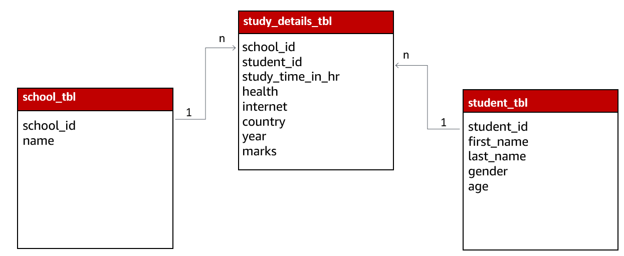
You can configure the parallel run of tasks and allocate resources for Kinesis Data Analytics for Apache Flink to implement scaling. We use the following properties:

  • Parallelism – Use this property to set the default Apache Flink application parallelism. All operators, sources, and sinks run with this parallelism unless overridden in the application code. The default is 1, and the default maximum is 256.
  • ParallelismPerKPU – Use this property to set the number of parallel tasks that can be scheduled per the of your application. The default is 1, and the maximum is 8. For applications that have blocking operations (for example, I/O), a higher value of ParallelismPerKPU leads to full utilization of KPU resources.

Kinesis Data Analytics calculates the KPUs needed to run your application as Parallelism/ParallelismPerKPU.

The following example request for the CreateApplication action sets parallelism when you create an application.

{
   "ApplicationName": "string",
   "RuntimeEnvironment":"FLINK-1_11",
   "ServiceExecutionRole":"arn:aws:iam::123456789123:role/myrole",
   "ApplicationConfiguration": { 
      "ApplicationCodeConfiguration":{
      "CodeContent":{
         "S3ContentLocation":{
            "BucketARN":"arn:aws:s3:::mybucket",
            "FileKey":"myflink.jar",
            "ObjectVersion":"AbCdEfGhIjKlMnOpQrStUvWxYz12345"
            }
         },
      "CodeContentType":"ZIPFILE"
   },   
      "FlinkApplicationConfiguration": { 
         "ParallelismConfiguration": { 
            "AutoScalingEnabled": "true",
            "ConfigurationType": "CUSTOM",
            "Parallelism": 4,
            "ParallelismPerKPU": 4
         }
      }
   }
}


For more examples and instructions for using request blocks with API actions, see Kinesis Data Analytics API Example Code.

The following example request for the UpdateApplication action sets parallelism for an existing application:

{
   "ApplicationName": "MyApplication",
   "CurrentApplicationVersionId": 4,
   "ApplicationConfigurationUpdate": { 
      "FlinkApplicationConfigurationUpdate": { 
         "ParallelismConfigurationUpdate": { 
            "AutoScalingEnabledUpdate": "true",
            "ConfigurationTypeUpdate": "CUSTOM",
            "ParallelismPerKPUUpdate": 4,
            "ParallelismUpdate": 4
         }
      }
   }
}

Scale the Kinesis Data Analytics for Apache Flink application

Because you increased the throughput of the Kinesis data stream by doubling the number of shards, more events are sent into the stream. However, as a direct result, more events need to be processed. Now the Kinesis data analytics application becomes overloaded and can no longer keep up with the increased number of incoming events. You can observe this through the millisBehindLatest metric, which is published to CloudWatch.

Kinesis Data Analytics natively supports auto scaling. After few minutes, you can see the effect of the auto scaling activities in the metrics. The millisBehindLatest metric starts to decrease until it reaches zero when the processing has caught up with the tip of the Kinesis data stream.

You can calibrate the scaling operation based on your application needs by adjusting the KPU.

  1. On the Kinesis Data Analytics console, navigate to your application.
  2. Under Scaling, choose Configure.
  3. Adjust Parallelism to 6 and Parallelism per KPU to 2.
  4. Choose Update.

The other method that you can apply to improve throughput is the AsyncIO function. You can make AsyncIO calls asynchronously to improve throughput while other requests are in progress. The two essential parameters when defining an AsyncFunction are Capacity (how many requests are in-flight concurrently per parallel sub-task) and Timeout (the timeout duration of an individual request to the external data source). It helps if you allocate enough capacity to account for the throughput, but not more than the external data source can handle. For example, application with a parallelism of 5 and a capacity of 10 sends 50 concurrent requests to your external data source. You can learn more about using the AsyncIO function with Kinesis Data Analytics for Apache Flink on the GitHub repo.

Conclusion

In this post, you built a reliable, scalable, and highly available streaming application based on Apache Flink and Kinesis Data Analytics. You also scaled the different components while ingesting and analyzing thousands of events per second in near-real time. The solution utilizes managed services without having to provision and configure underlying infrastructure. The post also discussed what it takes to auto scale your application based on metrics such as CPU utilization and millisBehindLatest. The sources of the AWS CloudFormation templates used in this post are available from GitHub for your reference.
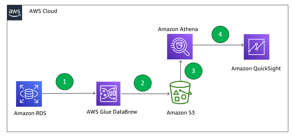
You now know how to build a real-time streaming application using Kinesis Data Analytics on AWS. You can also calibrate KPUs based on your application needs and volume of data. Check out Part 2 of this post to explore advanced monitoring techniques and auto scale your real-time streaming application, adapting with streaming data.


About the Author

Amit Chowdhury is a Partner Solutions Architect in the Global System Integrator (GSI) team at Amazon Web Services. He helps AWS GSI partners migrate customer workloads to AWS, and provides guidance to build, design, and architect scalable, highly available, and secure solutions on AWS by applying AWS recommended best practices. He enjoys spending time with his family, outdoor adventures and traveling.
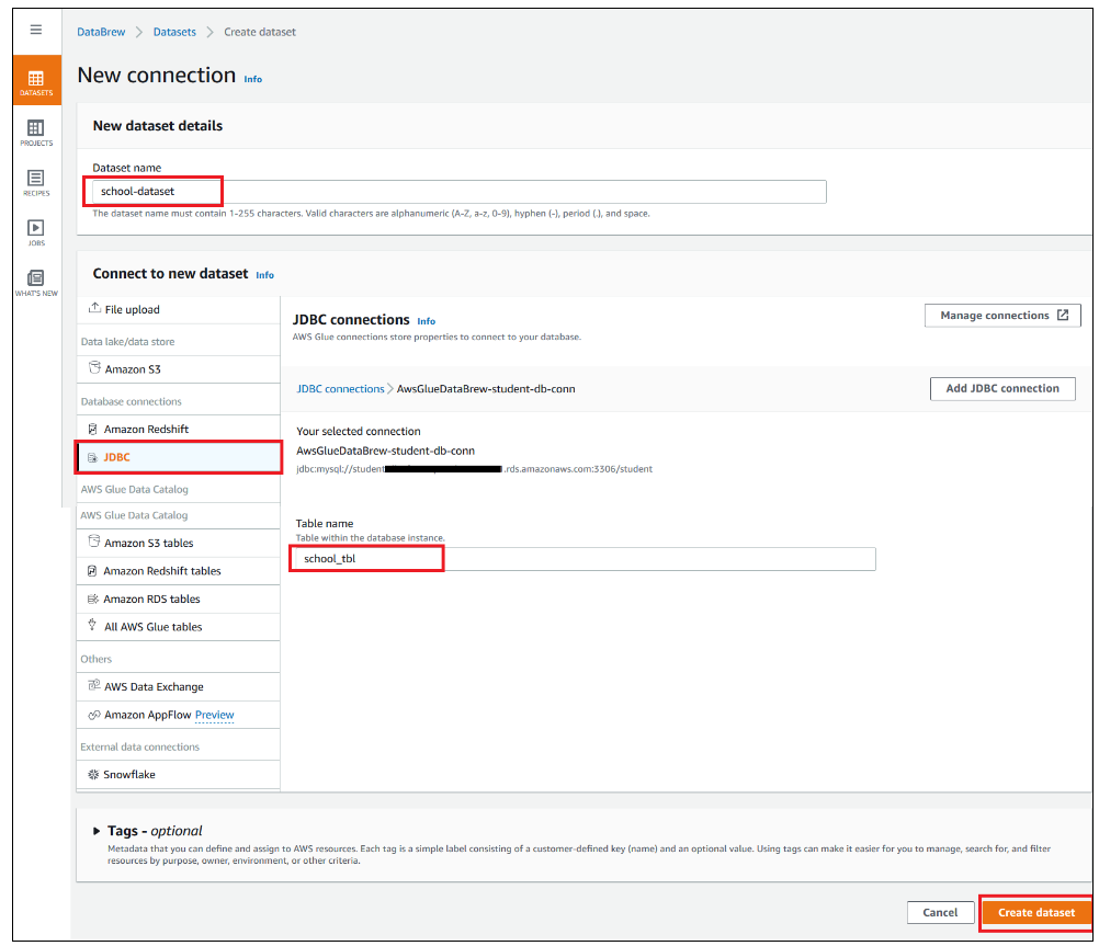
 

Saurabh Shrivastava is a solutions architect leader and analytics specialist working with global systems integrators. He works with AWS Partners and customers to provide them with architectural guidance for building scalable architecture in hybrid and AWS environments. He enjoys spending time with his family outdoors and traveling to new destinations to discover new cultures.