Tag Archives: Analytics

How Hudl built a cost-optimized AWS Glue pipeline with Apache Hudi datasets

Post Syndicated from Indira Balakrishnan original https://aws.amazon.com/blogs/big-data/how-hudl-built-a-cost-optimized-aws-glue-pipeline-with-apache-hudi-datasets/

This is a guest blog post co-written with Addison Higley and Ramzi Yassine from Hudl.

Hudl Agile Sports Technologies, Inc. is a Lincoln, Nebraska based company that provides tools for coaches and athletes to review game footage and improve individual and team play. Its initial product line served college and professional American football teams. Today, the company provides video services to youth, amateur, and professional teams in American football as well as other sports, including soccer, basketball, volleyball, and lacrosse. It now serves 170,000 teams in 50 different sports around the world. Hudl’s overall goal is to capture and bring value to every moment in sports.

Hudl’s mission is to make every moment in sports count. Hudl does this by expanding access to more moments through video and data and putting those moments in context. Our goal is to increase access by different people and increase context with more data points for every customer we serve. Using data to generate analytics, Hudl is able to turn data into actionable insights, telling powerful stories with video and data.

To best serve our customers and provide the most powerful insights possible, we need to be able to compare large sets of data between different sources. For example, enriching our MongoDB and Amazon DocumentDB (with MongoDB compatibility) data with our application logging data leads to new insights. This requires resilient data pipelines.

In this post, we discuss how Hudl has iterated on one such data pipeline using AWS Glue to improve performance and scalability. We talk about the initial architecture of this pipeline, and some of the limitations associated with this approach. We also discuss how we iterated on that design using Apache Hudi to dramatically improve performance.

Problem statement

A data pipeline that ensures high-quality MongoDB and Amazon DocumentDB statistics data is available in our central data lake, and is a requirement for Hudl to be able to deliver sports analytics. It’s important to maintain the integrity of the data between MongoDB and Amazon DocumentDB transactional data with the data lake capturing changes in near-real time along with upserts to records in the data lake. Because Hudl statistics are backed by MongoDB and Amazon DocumentDB databases, in addition to a broad range of other data sources, it’s important that relevant MongoDB and Amazon DocumentDB data is available in a central data lake where we can run analytics queries to compare statistics data between sources.

Initial design

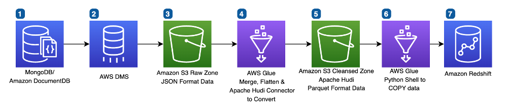
The following diagram demonstrates the architecture of our initial design.

Intial Ingestion Pipeline Design

Let’s discuss the key AWS services of this architecture:

  • AWS Data Migration Service (AWS DMS) allowed our team to move quickly in delivering this pipeline. AWS DMS gives our team a full snapshot of the data, and also offers ongoing change data capture (CDC). By combining these two datasets, we can ensure our pipeline delivers the latest data.
  • Amazon Simple Storage Service (Amazon S3) is the backbone of Hudl’s data lake because of its durability, scalability, and industry-leading performance.
  • AWS Glue allows us to run our Spark workloads in a serverless fashion, with minimal setup. We chose AWS Glue for its ease of use and speed of development. Additionally, features such as AWS Glue bookmarking simplified our file management logic.
  • Amazon Redshift offers petabyte-scale data warehousing. Amazon Redshift provides consistently fast performance, and easy integrations with our S3 data lake.

The data processing flow includes the following steps:

  1. Amazon DocumentDB holds the Hudl statistics data.
  2. AWS DMS gives us a full export of statistics data from Amazon DocumentDB, and ongoing changes in the same data.
  3. In the S3 Raw Zone, the data is stored in JSON format.
  4. An AWS Glue job merges the initial load of statistics data with the changed statistics data to give a snapshot of statistics data in JSON format for reference, eliminating duplicates.
  5. In the S3 Cleansed Zone, the JSON data is normalized and converted to Parquet format.
  6. AWS Glue uses a COPY command to insert Parquet data into Amazon Redshift consumption base tables.
  7. Amazon Redshift stores the final table for consumption.

The following is a sample code snippet from the AWS Glue job in the initial data pipeline:

from awsglue.context import GlueContext 
from pyspark.sql.session import SparkSession

spark = SparkSession.builder.getOrCreate() 
spark_context = spark.sparkContext 
gc = GlueContext(spark_context)
   full_df = read_full_data()#Load entire dataset from S3 Cleansed Zone


cdc_df = read_cdc_data() # Read new CDC data which represents delta in the source MongoDB/DocumentDB


joined_df = full_df.join(cdc_df, '_id', 'full_outer') #Calculate final snapshot by joining the existing data with delta


result = joined_df.filter((joined_df.Op != 'D') | (joined_df.Op.isNull())) .select(coalesce(cdc_df._doc, full_df._doc).alias('_doc'))

gc.write_dynamic_frame.from_options(frame=DynamicFrame.fromDF(result, gc) , connection_type = "s3", connection_options = {"path": output_path}, format = "parquet", transformation_ctx = "ctx4")

Challenges

Although this initial solution met our need for data quality, we felt there was room for improvement:

  • The pipeline was slow – The pipeline ran slowly (over 2 hours) because for each batch, the whole dataset was compared. Every record had to be compared, flattened, and converted to Parquet, even when only a few records were changed from the previous daily run.
  • The pipeline was expensive – As the data size grew daily, the job duration also grew significantly (especially in step 4). To mitigate the impact, we needed to allocate more AWS Glue DPUs (Data Processing Units) to scale the job, which led to higher cost.
  • The pipeline limited our ability to scale – Hudl’s data has a long history of rapid growth with increasing customers and sporting events. Given this trend, our pipeline needed to run as efficiently as possible to handle only changing datasets to have predictable performance.

New design

The following diagram illustrates our updated pipeline architecture.

Although the overall architecture looks roughly the same, the internal logic in AWS Glue was significantly changed, along with addition of Apache Hudi datasets.

In step 4, AWS Glue now interacts with Apache HUDI datasets in the S3 Cleansed Zone to upsert or delete changed records as identified by AWS DMS CDC. The AWS Glue to Apache Hudi connector helps convert JSON data to Parquet format and upserts into the Apache HUDI dataset. Retaining the full documents in our Apache HUDI dataset allows us to easily make schema changes to our final Amazon Redshift tables without needing to re-export data from our source systems.

The following is a sample code snippet from the new AWS Glue pipeline:

from awsglue.context import GlueContext 
from pyspark.sql.session import SparkSession

spark = SparkSession.builder.getOrCreate() 
spark_context = spark.sparkContext 
gc = GlueContext(spark_context)

upsert_conf = {'className': 'org.apache.hudi', '
hoodie.datasource.hive_sync.use_jdbc': 'false', 
'hoodie.datasource.write.precombine.field': 'write_ts', 
'hoodie.datasource.write.recordkey.field': '_id', 
'hoodie.table.name': 'glue_table', 
'hoodie.consistency.check.enabled': 'true', 
'hoodie.datasource.hive_sync.database': 'glue_database', 'hoodie.datasource.hive_sync.table': 'glue_table', 'hoodie.datasource.hive_sync.enable': 'true', 'hoodie.datasource.hive_sync.support_timestamp': 'true', 'hoodie.datasource.hive_sync.sync_as_datasource': 'false', 
'path': 's3://bucket/prefix/', 'hoodie.compact.inline': 'false', 'hoodie.datasource.hive_sync.partition_extractor_class':'org.apache.hudi.hive.NonPartitionedExtractor, 'hoodie.datasource.write.keygenerator.class': 'org.apache.hudi.keygen.NonpartitionedKeyGenerator', 'hoodie.upsert.shuffle.parallelism': 200, 
'hoodie.datasource.write.operation': 'upsert', 
'hoodie.cleaner.policy': 'KEEP_LATEST_COMMITS', 
'hoodie.cleaner.commits.retained': 10 }

gc.write_dynamic_frame.from_options(frame=DynamicFrame.fromDF(cdc_upserts_df, gc, "cdc_upserts_df"), connection_type="marketplace.spark", connection_options=upsert_conf)

Results

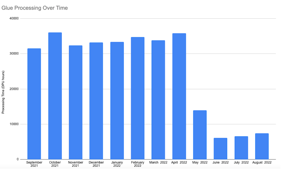
With this new approach using Apache Hudi datasets with AWS Glue deployed after May 2022, the pipeline runtime was predictable and less expensive than the initial approach. Because we only handled new or modified records by eliminating the full outer join over the entire dataset, we saw an 80–90% reduction in runtime for this pipeline, thereby reducing costs by 80–90% compared to the initial approach. The following diagram illustrates our processing time before and after implementing the new pipeline.

Conclusion

With Apache Hudi’s open-source data management framework, we simplified incremental data processing in our AWS Glue data pipeline to manage data changes at the record level in our S3 data lake with CDC from Amazon DocumentDB.

We hope that this post will inspire your organization to build AWS Glue pipelines with Apache Hudi datasets that reduce cost and bring performance improvements using serverless technologies to achieve your business goals.


About the authors

Addison Higley is a Senior Data Engineer at Hudl. He manages over 20 data pipelines to help ensure data is available for analytics so Hudl can deliver insights to customers.

Ramzi Yassine is a Lead Data Engineer at Hudl. He leads the architecture, implementation of Hudl’s data pipelines and data applications, and ensures that our data empowers internal and external analytics.

Swagat Kulkarni is a Senior Solutions Architect at AWS and an AI/ML enthusiast. He is passionate about solving real-world problems for customers with cloud-native services and machine learning. Swagat has over 15 years of experience delivering several digital transformation initiatives for customers across multiple domains, including retail, travel and hospitality, and healthcare. Outside of work, Swagat enjoys travel, reading, and meditating.

Indira Balakrishnan is a Principal Solutions Architect in the AWS Analytics Specialist SA Team. She is passionate about helping customers build cloud-based analytics solutions to solve their business problems using data-driven decisions. Outside of work, she volunteers at her kids’ activities and spends time with her family.

How SOCAR built a streaming data pipeline to process IoT data for real-time analytics and control

Post Syndicated from DoYeun Kim original https://aws.amazon.com/blogs/big-data/how-socar-built-a-streaming-data-pipeline-to-process-iot-data-for-real-time-analytics-and-control/

SOCAR is the leading Korean mobility company with strong competitiveness in car-sharing. SOCAR has become a comprehensive mobility platform in collaboration with Nine2One, an e-bike sharing service, and Modu Company, an online parking platform. Backed by advanced technology and data, SOCAR solves mobility-related social problems, such as parking difficulties and traffic congestion, and changes the car ownership-oriented mobility habits in Korea.

SOCAR is building a new fleet management system to manage the many actions and processes that must occur in order for fleet vehicles to run on time, within budget, and at maximum efficiency. To achieve this, SOCAR is looking to build a highly scalable data platform using AWS services to collect, process, store, and analyze internet of things (IoT) streaming data from various vehicle devices and historical operational data.

This in-car device data, combined with operational data such as car details and reservation details, will provide a foundation for analytics use cases. For example, SOCAR will be able to notify customers if they have forgotten to turn their headlights off or to schedule a service if a battery is running low. Unfortunately, the previous architecture didn’t enable the enrichment of IoT data with operational data and couldn’t support streaming analytics use cases.

AWS Data Lab offers accelerated, joint-engineering engagements between customers and AWS technical resources to create tangible deliverables that accelerate data and analytics modernization initiatives. The Build Lab is a 2–5-day intensive build with a technical customer team.

In this post, we share how SOCAR engaged the Data Lab program to assist them in building a prototype solution to overcome these challenges, and to build the basis for accelerating their data project.

Use case 1: Streaming data analytics and real-time control

SOCAR wanted to utilize IoT data for a new business initiative. A fleet management system, where data comes from IoT devices in the vehicles, is a key input to drive business decisions and derive insights. This data is captured by AWS IoT and sent to Amazon Managed Streaming for Apache Kafka (Amazon MSK). By joining the IoT data to other operational datasets, including reservations, car information, device information, and others, the solution can support a number of functions across SOCAR’s business.

An example of real-time monitoring is when a customer turns off the car engine and closes the car door, but the headlights are still on. By using IoT data related to the car light, door, and engine, a notification is sent to the customer to inform them that the car headlights should be turned off.

Although this real-time control is important, they also want to collect historical data—both raw and curated data—in Amazon Simple Storage Service (Amazon S3) to support historical analytics and visualizations by using Amazon QuickSight.

Use case 2: Detect table schema change

The first challenge SOCAR faced was existing batch ingestion pipelines that were prone to breaking when schema changes occurred in the source systems. Additionally, these pipelines didn’t deliver data in a way that was easy for business analysts to consume. In order to meet the future data volumes and business requirements, they needed a pattern for the automated monitoring of batch pipelines with notification of schema changes and the ability to continue processing.

The second challenge was related to the complexity of the JSON files being ingested. The existing batch pipelines weren’t flattening the five-level nested structure, which made it difficult for business users and analysts to gain business insights without any effort on their end.

Overview of solution

In this solution, we followed the serverless data architecture to establish a data platform for SOCAR. This serverless architecture allowed SOCAR to run data pipelines continuously and scale automatically with no setup cost and without managing servers.

AWS Glue is used for both the streaming and batch data pipelines. Amazon Kinesis Data Analytics is used to deliver streaming data with subsecond latencies. In terms of storage, data is stored in Amazon S3 for historical data analysis, auditing, and backup. However, when frequent reading of the latest snapshot data is required by multiple users and applications concurrently, the data is stored and read from Amazon DynamoDB tables. DynamoDB is a key-value and document database that can support tables of virtually any size with horizontal scaling.

Let’s discuss the components of the solution in detail before walking through the steps of the entire data flow.

Component 1: Processing IoT streaming data with business data

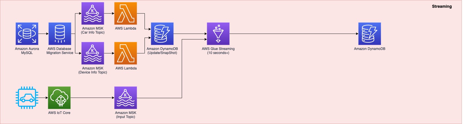
The first data pipeline (see the following diagram) processes IoT streaming data with business data from an Amazon Aurora MySQL-Compatible Edition database.

Whenever a transaction occurs in two tables in the Aurora MySQL database, this transaction is captured as data and then loaded into two MSK topics via AWS Database Management (AWS DMS) tasks. One topic conveys the car information table, and the other topic is for the device information table. This data is loaded into a single DynamoDB table that contains all the attributes (or columns) that exist in the two tables in the Aurora MySQL database, along with a primary key. This single DynamoDB table contains the latest snapshot data from the two DB tables, and is important because it contains the latest information of all the cars and devices for the lookup against the streaming IoT data. If the lookup were done on the database directly with the streaming data, it would impact the production database performance.

When the snapshot is available in DynamoDB, an AWS Glue streaming job runs continuously to collect the IoT data and join it with the latest snapshot data in the DynamoDB table to produce the up-to-date output, which is written into another DynamoDB table.

The up-to-date data in DynamoDB is used for real-time monitoring and control that SOCAR’s Data Analytics team performs for safety maintenance and fleet management. This data is ultimately consumed by a number of apps to perform various business activities, including route optimization, real-time monitoring for oil consumption and temperature, and to identify a driver’s driving pattern, tire wear and defect detection, and real-time car crash notifications.

Component 2: Processing IoT data and visualizing the data in dashboards

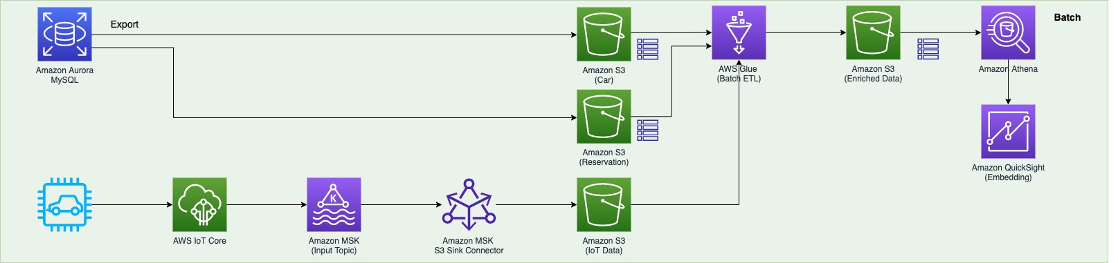
The second data pipeline (see the following diagram) batch processes the IoT data and visualizes it in QuickSight dashboards.

There are two data sources. The first is the Aurora MySQL database. The two database tables are exported into Amazon S3 from the Aurora MySQL cluster and registered in the AWS Glue Data Catalog as tables. The second data source is Amazon MSK, which receives streaming data from AWS IoT Core. This requires you to create a secure AWS Glue connection for an Apache Kafka data stream. SOCAR’s MSK cluster requires SASL_SSL as a security protocol (for more information, refer to Authentication and authorization for Apache Kafka APIs). To create an MSK connection in AWS Glue and set up connectivity, we use the following CLI command:

aws glue create-connection —connection-input
'{"Name":"kafka-connection","Description":"kafka connection example",
"ConnectionType":"KAFKA",
"ConnectionProperties":{
"KAFKA_BOOTSTRAP_SERVERS":"<server-ip-addresses>",
"KAFKA_SSL_ENABLED":"true",
// "KAFKA_CUSTOM_CERT": "s3://bucket/prefix/cert.pem",
"KAFKA_SECURITY_PROTOCOL" : "SASL_SSL",
"KAFKA_SKIP_CUSTOM_CERT_VALIDATION":"false",
"KAFKA_SASL_MECHANISM": "SCRAM-SHA-512",
"KAFKA_SASL_SCRAM_USERNAME": "<username>",
"KAFKA_SASL_SCRAM_PASSWORD: "<password>"
},
"PhysicalConnectionRequirements":
{"SubnetId":"subnet-xxx","SecurityGroupIdList":["sg-xxx"],"AvailabilityZone":"us-east-1a"}}'

Component 3: Real-time control

The third data pipeline processes the streaming IoT data in millisecond latency from Amazon MSK to produce the output in DynamoDB, and sends a notification in real time if any records are identified as an outlier based on business rules.

AWS IoT Core provides integrations with Amazon MSK to set up real-time streaming data pipelines. To do so, complete the following steps:

  1. On the AWS IoT Core console, choose Act in the navigation pane.
  2. Choose Rules, and create a new rule.
  3. For Actions, choose Add action and choose Kafka.
  4. Choose the VPC destination if required.
  5. Specify the Kafka topic.
  6. Specify the TLS bootstrap servers of your Amazon MSK cluster.

You can view the bootstrap server URLs in the client information of your MSK cluster details. The AWS IoT rule was created with the Kafka topic as an action to provide data from AWS IoT Core to Kafka topics.

SOCAR used Amazon Kinesis Data Analytics Studio to analyze streaming data in real time and build stream-processing applications using standard SQL and Python. We created one table from the Kafka topic using the following code:

CREATE TABLE table_name (
column_name1 VARCHAR,
column_name2 VARCHAR(100),
column_name3 VARCHAR,
column_name4 as TO_TIMESTAMP (`time_column`, 'EEE MMM dd HH:mm:ss z yyyy'),
 WATERMARK FOR column AS column -INTERVAL '5' SECOND
)
PARTITIONED BY (column_name5)
WITH (
'connector'= 'kafka',
'topic' = 'topic_name',
'properties.bootstrap.servers' = '<bootstrap servers shown in the MSK client info dialog>',
'format' = 'json',
'properties.group.id' = 'testGroup1',
'scan.startup.mode'= 'earliest-offset'
);

Then we applied a query with business logic to identify a particular set of records that need to be alerted. When this data is loaded back into another Kafka topic, AWS Lambda functions trigger the downstream action: either load the data into a DynamoDB table or send an email notification.

Component 4: Flattening the nested structure JSON and monitoring schema changes

The final data pipeline (see the following diagram) processes complex, semi-structured, and nested JSON files.

This step uses an AWS Glue DynamicFrame to flatten the nested structure and then land the output in Amazon S3. After the data is loaded, it’s scanned by an AWS Glue crawler to update the Data Catalog table and detect any changes in the schema.

Data flow: Putting it all together

The following diagram illustrates our complete data flow with each component.

Let’s walk through the steps of each pipeline.

The first data pipeline (in red) processes the IoT streaming data with the Aurora MySQL business data:

  1. AWS DMS is used for ongoing replication to continuously apply source changes to the target with minimal latency. The source includes two tables in the Aurora MySQL database tables (carinfo and deviceinfo), and each is linked to two MSK topics via AWS DMS tasks.
  2. Amazon MSK triggers a Lambda function, so whenever a topic receives data, a Lambda function runs to load data into DynamoDB table.
  3. There is a single DynamoDB table with columns that exist from the carinfo table and the deviceinfo table of the Aurora MySQL database. This table consists of all the data from two tables and stores the latest data by performing an upsert operation.
  4. An AWS Glue job continuously receives the IoT data and joins it with data in the DynamoDB table to produce the output into another DynamoDB target table.
  5. This target table contains the final data, which includes all the device and car status information from the IoT devices as well as metadata from the Aurora MySQL table.

The second data pipeline (in green) batch processes IoT data to use in dashboards and for visualization:

  1. The car and reservation data (in two DB tables) is exported via a SQL command from the Aurora MySQL database with the output data available in an S3 bucket. The folders that contain data are registered as an S3 location for the AWS Glue crawler and become available via the AWS Glue Data Catalog.
  2. The MSK input topic continuously receives data from AWS IoT. Each car has a number of IoT devices, and each device captures data and sends it to an MSK input topic. The Amazon MSK S3 sink connector is configured to export data from Kafka topics to Amazon S3 in JSON formats. In addition, the S3 connector exports data by guaranteeing exactly-once delivery semantics to consumers of the S3 objects it produces.
  3. The AWS Glue job runs in a daily batch to load the historical IoT data into Amazon S3 and into two tables (refer to step 1) to produce the output data in an Enriched folder in Amazon S3.
  4. Amazon Athena is used to query data from Amazon S3 and make it available as a dataset in QuickSight for visualizing historical data.

The third data pipeline (in blue) processes streaming IoT data from Amazon MSK with millisecond latency to produce the output in DynamoDB and send a notification:

  1. An Amazon Kinesis Data Analytics Studio notebook powered by Apache Zeppelin and Apache Flink is used to build and deploy its output as a Kinesis Data Analytics application. This application loads data from Amazon MSK in real time, and users can apply business logic to select particular events coming from the IoT real-time data, for example, the car engine is off and the doors are closed, but the headlights are still on. The particular event that users want to capture can be sent to another MSK topic (Outlier) via the Kinesis Data Analytics application.
  2. Amazon MSK triggers a Lambda function, so whenever a topic receives data, a Lambda function runs to send an email notification to users that are subscribed to an Amazon Simple Notification Service (Amazon SNS) topic. An email is published using an SNS notification.
  3. The Kinesis Data Analytics application loads data from AWS IoT, applies business logic, and then loads it into another MSK topic (output). Amazon MSK triggers a Lambda function when data is received, which loads data into a DynamoDB Append table.
  4. Amazon Kinesis Data Analytics Studio is used to run SQL commands for ad hoc interactive analysis on streaming data.

The final data pipeline (in yellow) processes complex, semi-structured, and nested JSON files, and sends a notification when a schema evolves.

  1. An AWS Glue job runs and reads the JSON data from Amazon S3 (as a source), applies logic to flatten the nested schema using a DynamicFrame, and pivots out array columns from the flattened frame.
  2. The output is stored in Amazon S3 and is automatically registered to the AWS Glue Data Catalog table.
  3. Whenever there is a new attribute or change in the JSON input data at any level in the nested structure, the new attribute and change are captured in Amazon EventBridge as an event from the AWS Glue Data Catalog. An email notification is published using Amazon SNS.

Conclusion

As a result of the four-day Build Lab, the SOCAR team left with a working prototype that is custom fit to their needs, gaining a clear path to production. The Data Lab allowed the SOCAR team to build a new streaming data pipeline, enrich IoT data with operational data, and enhance the existing data pipeline to process complex nested JSON data. This establishes a baseline architecture to support the new fleet management system beyond the car-sharing business.


About the Authors

DoYeun Kim is the Head of Data Engineering at SOCAR. He is a passionate software engineering professional with 19+ years experience. He leads a team of 10+ engineers who are responsible for the data platform, data warehouse and MLOps engineering, as well as building in-house data products.

SangSu Park is a Lead Data Architect in SOCAR’s cloud DB team. His passion is to keep learning, embrace challenges, and strive for mutual growth through communication. He loves to travel in search of new cities and places.

YoungMin Park is a Lead Architect in SOCAR’s cloud infrastructure team. His philosophy in life is-whatever it may be-to challenge, fail, learn, and share such experiences to build a better tomorrow for the world. He enjoys building expertise in various fields and basketball.

Younggu Yun is a Senior Data Lab Architect at AWS. He works with customers around the APAC region to help them achieve business goals and solve technical problems by providing prescriptive architectural guidance, sharing best practices, and building innovative solutions together. In his free time, his son and he are obsessed with Lego blocks to build creative models.

Vicky Falconer leads the AWS Data Lab program across APAC, offering accelerated joint engineering engagements between teams of customer builders and AWS technical resources to create tangible deliverables that accelerate data analytics modernization and machine learning initiatives.

Learn more about Apache Flink and Amazon Kinesis Data Analytics with three new videos

Post Syndicated from Deepthi Mohan original https://aws.amazon.com/blogs/big-data/learn-more-about-apache-flink-and-amazon-kinesis-data-analytics-with-three-new-videos/

Amazon Kinesis Data Analytics is a fully managed service for Apache Flink that reduces the complexity of building, managing, and integrating Apache Flink applications with other AWS services. Apache Flink is an open-source framework and engine for stateful processing of data streams. It’s highly available and scalable, delivering high throughput and low latency for the most demanding stream-processing applications.

In this post, we highlight three new videos for you to learn more about Apache Flink and Kinesis Data Analytics, including open-source contributions to Apache Flink, our learnings from running thousands of Flink jobs on a managed service, and how we use Kinesis Data Analytics and Apache Flink to enable machine learning (ML) in Alexa.

In Introducing the new Async Sink, we present the new Async Sink framework, an open-source contribution to make it easier than ever to build sink connectors for Apache Flink. You can learn about the need for the Async Sink framework and how we built it, followed by a demo of building a new sink to Amazon CloudWatch to deliver CloudWatch metrics, in under 20 minutes! The Async Sink framework bootstraps development of Flink sinks, is compatible with Apache Flink 1.15 and above, and has already seen usage by the community beyond building new sinks to AWS services.

The video Practical learnings from running thousands of Flink jobs shares insight from running Kinesis Data Analytics, a managed service for Apache Flink that runs tens of thousands of Flink jobs. You can learn lessons based on our experience of operating Apache Flink at very large scale, touching on issues such as out-of-memory errors, timeouts, and stability challenges. The video also covers improving application performance with memory tuning and configuration changes and the approaches to automating job health monitoring and management of Flink jobs at scale.

“Alexa, be quiet!” End-to-end near-real time model building and evaluation in Amazon Alexa discusses how Alexa has built an automated end-to-end solution for incremental model building or fine-tuning ML models through continuous learning, continual learning, or semi-supervised active learning. Alexa uses Apache Flink to transform and discover metrics in real time. In this video, you learn about how Alexa scales infrastructure to meet the needs of ML teams across Alexa, and explore specific use cases that use Apache Flink and Kinesis Data Analytics to improve Alexa experiences to delight customers.

To learn more about Kinesis Data Analytics for Apache Flink, visit our product page.


About the author

Deepthi Mohan is a Principal Product Manager on the Kinesis Data Analytics team.

How Kyligence Cloud uses Amazon EMR Serverless to simplify OLAP

Post Syndicated from Daniel Gu original https://aws.amazon.com/blogs/big-data/how-kyligence-cloud-uses-amazon-emr-serverless-to-simplify-olap/

This post was co-written with Daniel Gu and Yolanda Wang, from Kyligence.

Today, more than ever, organizations realize that modern business runs on data—almost all our interactions with business are based on data, and organizations must use analytics to understand, plan, and improve their operations. That is where Online Analytical Processing (OLAP) comes in. OLAP is designed to manage and analyze big data, enabling organizations to use their data to extract business insights in multiple dimensions.

Kyligence Cloud OLAP solution offers an Intelligent OLAP Platform to simplify multi-dimensional analytics for cloud data lakes. In the past, Kyligence used to deploy and maintain its own Spark clusters based on Amazon Elastic Compute Cloud (Amazon EC2) to handle the multi-dimensional model pre-computing process that required users to build their monitoring and alerting systems to improve the observability and reliability of the Spark cluster. In this post, we present how Kyligence built and end-to-end Kyligence Cloud OLAP solution with Amazon EMR Serverless to simplify deployment and operations, reduce costs, and accelerate time-to-value over the data lake.

What is Amazon EMR Serverless?

Amazon EMR Serverless is a big data cloud platform for running large-scale distributed data processing jobs, and machine learning (ML) applications using open-source analytics frameworks like Apache Spark and Apache Hive. Amazon EMR Serverless makes it easy and cost-effective for data engineers and analysts to run applications without having to tune, operate, optimize, secure, or manage clusters.

What is OLAP?

OLAP is an approach to quickly answer analytics queries at high speeds on large volumes of data, providing capabilities for precomputation, sophisticated data modeling, and multi-dimensional analytics by rolling up large, sometimes separate datasets into a multi-dimensional database known as an OLAP Cube that enables “slicing and dicing” of data from different viewpoints for a streamlined query experience. Apache Kylin, Apache Druid, and ClickHouse are some of the popular OLAP tools.

Although OLAP tools have been successfully used in various industries, they still face many challenges:

  • Dependence on IT organizations – Traditional OLAP tools require complex infrastructure to run large-scale data computing. It requires a large team of IT professionals to operate and maintain this infrastructure, resulting in high costs.
  • Need for large compute resources – Traditional OLAP tools need huge amount of computing resources for processing, and transforming data through a series of specific steps toward a concrete goal. Lack of computational capabilities leads to longer response times, limits the amount of data that can be processed, and impedes the flexibility of the OLAP tool greatly . As a result, data analysts are often confined to narrow datasets, incapable of analyzing all the data freely.
  • Inefficient usage of resources in the cloud – When a large-scale data modeling calculation is performed in the cloud, the cost estimation tools estimate and deploy the corresponding computing resources. However, the utilization rate of resources is often not very high, resulting in inefficient usage of resources.

With OLAP integrated with Amazon EMR Serverless, OLAP tools can use Amazon EMR Serverless as a serverless computing resource pool to complete data processing jobs, which simplifies and enhances user experience.

Kyligence approach to OLAP using Amazon EMR Serverless

Kyligence is an AWS ISV partner that offers an Intelligent OLAP Platform to simplify multi-dimensional analytics for cloud data lakes. As a cloud-native OLAP platform, Kyligence Cloud now integrates with Amazon EMR Serverless to automatically provision Spark to run indexing and building jobs. This empowers you to use all the features and benefits of Kyligence’s OLAP with Amazon EMR Serverless.

Kyligence seamlessly connects to major AWS-native data sources including Amazon Simple Storage Service (Amazon S3), Amazon Redshift, and Amazon Relational Database Service (Amazon RDS) to get the most out of your data on AWS, building a comprehensive AWS big data solution. During data modeling, Kyligence uses Amazon S3 to store the pre-computed data, and serves it for high concurrency queries. Kyligence also seamlessly interfaces with popular business intelligence (BI) tools such as Tableau, Microsoft Power BI, and Microsoft Excel to provide rich, built-in data visualization and self-service tools.

The following diagram illustrates the Kyligence Cloud architecture on AWS.

What you can expect from Kyligence Cloud on AWS

This solution offers the following benefits:

  • High performance – With AWS’s global infrastructure and the distributed computing capabilities of Amazon EMR, Kyligence offers a scalable, cost-effective, high-performance OLAP engine for multi-dimensional analytics. It enables critical data applications and large-scale interactive analytics, and helps you achieve sub-second query response times and high concurrency on PB-scale data.
  • Auto-scaling – Kyligence Cloud’s computing resources can be expanded with one click, and as load decreases, cluster size can be automatically reduced. This auto-scaling capability provides optimized costs with service stability.
  • High compatibility – Kyligence Cloud provides a rich set of APIs (ODBC, JDBC, Rest API, Python Client) and standard ANSI-SQL and XMLA/MDX interface, which can be easily integrated with popular analytics tools like Tableau, Microsoft Excel, Microsoft Power BI, and data science tools like Python.
  • Security and reliability – With Amazon S3, Amazon RDS, Kyligence enterprise-level security features, and AWS Identity and Access Management (IAM) support, Kyligence Cloud safely manages access to the services and resources deployed on AWS while supporting multi-level access control of data models, tables, and cells to ensure data security and privacy protection.
  • One-click deployment on AWS – Kyligence Cloud is available in AWS Marketplace. The deployment is completed automatically based on an AWS CloudFormation template and parameter settings. Kyligence performs automated cluster operation and maintenance, and elastic rule-based cluster scaling, which lightens the workload for IT administrators and cloud infrastructure teams. Kyligence also offers a quick deployment method in the Kyligence Cloud Portal.

How Amazon EMR Serverless integrates with OLAP

With Amazon EMR Serverless, Kyligence Cloud provides out-of-the-box managed Apache Spark services. The Kyligence engine can distribute the compute job to Apache Spark in Amazon EMR Serverless. With the automatic on-demand provisioning and scaling capabilities of Amazon EMR Serverless, Kyligence can quickly meet changing processing requirements at any data volume.

The following diagram illustrates Kyligence Cloud integrated with Amazon EMR Serverless.

Benefits of using Kyligence Cloud with Amazon EMR Serverless

In the past, Kyligence used to deploy and maintain its own Spark clusters based on Amazon Elastic Compute Cloud (Amazon EC2) to handle the multi-dimensional model pre-computing process that required Kyligence users to build their monitoring and alerting systems to improve the observability and reliability of the Spark clusters.

Now, running Kyligence on Amazon EMR Serverless offers a more cost-effective, and high-performance way to run cloud analytics on AWS:

  • Simplified deployment on the cloud – With managed services, you don’t need to consider the lifecycle of the underlying infrastructure and resources. This greatly reduces application complexity and simplifies the deployment of Kyligence Cloud.
  • Improve performance on the cloud – With the help of Amazon EMR Serverless, it provides a refined scaling strategy, which can help Kyligence Cloud spin up and recycle resources faster. In Kyligence performance benchmark testing, we observed 15–20% faster performance compared to open-source Spark cluster for index building.
  • Reduce the difficulty of operation and maintenance – With the help of Amazon EMR Serverless capabilities, operation and maintenance personnel can easily maintain the capacity and running status of computing resources without having to understand the underlying analysis framework.
  • Cost-optimization on the cloud – Amazon EMR Serverless provides a refined scaling strategy that can automatically determine the resources that the application needs, acquires these resources to process your jobs, and releases the resources when the jobs complete. You only pay for the resources used by the application, which helps reduce the Total Cost of Operations (TCO) on the cloud.

Get started with Kyligence Cloud on Amazon EMR Serverless

You can get started with the full potential of Kyligence Cloud on the AWS Marketplace or quickly test drive Kyligence.

To use Amazon EMR Serverless, you just need to select Serverless Spark on the Build Cluster tab during deployment.

Conclusion

Using managed and scalable services like Amazon EMR Serverless allows Kyligence users to speed up self-service analytics on large volumes of data, and maintain a relatively simplified architecture. With this solution, you can now concentrate on business demands instead of technical issues.

About Kyligence

Kyligence was founded in 2016 by the original creators of Apache Kylin™, the leading open-source OLAP for big data. Kyligence offers an Intelligent OLAP Platform to simplify multi-dimensional analytics for cloud data lakes.

For more information, visit Kyligence.


About the authors

Daniel Gu is a senior product manager on the Kyligence Cloud Team, who manages products and services and conducts research to determine the viability of products in the cloud.

Yolanda Wang is a senior product marketing manager at Kyligence, who owns the positioning, messaging, and branding of Kyligence products and works with various teams to drive go-to-market strategies.

Kiran Guduguntla is a WW Go-to-Market Specialist for Amazon EMR at AWS. He works with AWS customers across the globe to strategize, build, develop, and deploy modern data analytics solutions.

Field-level security in Amazon OpenSearch Service

Post Syndicated from Satyanarayana Adimula original https://aws.amazon.com/blogs/big-data/field-level-security-in-amazon-opensearch-service/

Amazon OpenSearch Service is fully open-source search and analytics engine that securely unlocks real-time search, monitoring, and analysis of business and operational data for use cases like application monitoring, log analytics, observability, and website search.

But what if you have personal identifiable information (PII) data in your log data? How do you control and audit access to that data? For example, what if you need to exclude fields from log search results or anonymize them? Fine-grained access control can manage access to your data depending on the use case—to return results from only one index, hide certain fields in your documents, or exclude certain documents altogether.

Let’s say you have users that work on the logistics of online orders placed on Sunday. The users must not have the access to a customer’s PII data and must be restricted from seeing the customer’s email. Additionally, the customer’s full name and first name must be anonymized. The post demonstrates implementing this field-level security with OpenSearch Service security controls.

Solution overview

The solution has the following steps to provision OpenSearch Service with Amazon Cognito federation within Amazon Virtual Private Cloud (Amazon VPC), use a proxy server to sign in to OpenSearch Dashboards, and demonstrate the field-level security:

  1. Create an OpenSearch Service domain with VPC access and fine-grained access enabled.
  2. Access OpenSearch Service from outside the VPC and load the sample data.
  3. Create an OpenSearch Service role for field-level security and map it to a backend role.

OpenSearch Service security has three main layers:

  • Network – Determines whether a request can reach an OpenSearch Service domain. Placing an OpenSearch Service domain within a VPC enables secure communication between OpenSearch Service and other services within the VPC without the need for an internet gateway, NAT device, or VPN connection. The associated security groups must permit clients to reach the OpenSearch Service endpoint.
  • Domain access policy – After a request reaches a domain endpoint, the domain access policy allows or denies the request access to a given URI at the edge of the domain. The domain access policy specifies which actions a principal can perform on the domain’s sub-resources, which include OpenSearch Service indexes and APIs. If a domain access policy contains AWS Identity and Access Management (IAM) users or roles, clients must send signed requests using AWS Signature Version 4.
  • Fine-grained access control – After the domain access policy allows a request to reach a domain endpoint, fine-grained access control evaluates the user credentials and either authenticates the user or denies the request. If fine-grained access control authenticates the user, the request is handled based on the OpenSearch Service roles mapped to the user. Additional security levels include:
    • Cluster-level security – To make broad requests such as _mget, _msearch, and _bulk, monitor health, take snapshots, and more. For details, see Cluster permissions.
    • Index-level security – To create new indexes, search indexes, read and write documents, delete documents, manage aliases, and more. For details, see Index permissions.
    • Document-level security – To restrict the documents in an index that a user can see. For details, see Document-level security.
    • Field-level security – To control the document fields a user can see. When creating a role, add a list of fields to either include or exclude. If you include fields, any users you map to that role can see only those fields. If you exclude fields, they can see all fields except the excluded ones. Field-level security affects the number of fields included in hits when you search. For details, see Field-level security.
    • Field masking – To anonymize the data in a field. If you apply the standard masking to a field, OpenSearch Service uses a secure, random hash that can cause inaccurate aggregation results. To perform aggregations on masked fields, use pattern-based masking instead. For details, see Field masking.

The following figure illustrates these layers.

Prerequisites

For this walkthrough, you should have the following prerequisites:

  • An AWS account
  • An Amazon Cognito user pool and identity pool

Create an OpenSearch Service domain with VPC access

You first create an OpenSearch Service domain with VPC access, enabling fine-grained access control and choosing the IAM ARN as the master user.

When you use IAM for the master user, all requests to the cluster must be signed using AWS Signature Version 4. For sample code, see Signing HTTP requests to Amazon OpenSearch Service. IAM is recommended if you want to use the same users on multiple clusters, to use Amazon Cognito to access OpenSearch Dashboards, or if you have OpenSearch Service clients that support Signature Version 4 signing.

Fine-grained access control requires HTTPS, node-to-node encryption, and encryption at rest. Node-to-node encryption enables TLS 1.2 encryption for all communications within the VPC. If you send data to OpenSearch Service over HTTPS, node-to-node encryption helps ensure that your data remains encrypted as OpenSearch Service distributes (and redistributes) it throughout the cluster.

Add a domain access policy to allow the specified IAM ARNs to the URI at the edge of the domain.

Set up Amazon Cognito to federate into OpenSearch Service

You can authenticate and protect your OpenSearch Service default installation of OpenSearch Dashboards using Amazon Cognito. If you don’t configure Amazon Cognito authentication, you can still protect Dashboards using an IP-based access policy and a proxy server, HTTP basic authentication, or SAML. For more details, see Amazon Cognito authentication for OpenSearch Dashboards.

Create a user called masteruser in the Amazon Cognito user pool that was configured for the OpenSearch Service domain and associate the user with the IAM role Cognito_<Cognito User Pool>Auth_Role, which is a master user in OpenSearch Service. Create another user called ecomuser1 and associate it with a different IAM role, for example OpenSearchFineGrainedAccessRole. Note that ecomuser1 doesn’t have any access by default.

If you want to configure SAML authentication, see SAML authentication for OpenSearch Dashboards.

Access OpenSearch Service from outside the VPC

When you place your OpenSearch Service domain within a VPC, your computer must be able to connect to the VPC. This connection can be VPN, transit gateway, managed network, or proxy server.

Fine-grained access control has an OpenSearch Dashboards plugin that simplifies management tasks. You can use Dashboards to manage users, roles, mappings, action groups, and tenants. The Dashboards sign-in page and underlying authentication method differs depending on how you manage users and configured your domain.

Load sample data into OpenSearch

Sign in as masteruser to access OpenSearch Dashboards and load the sample data for ecommerce orders, flight data, and web logs.

Create an OpenSearch Service role and user mapping

OpenSearch Service roles are the core ways of controlling access to your cluster. Roles contain any combination of cluster-wide permissions, index-specific permissions, document-level and field-level security, and tenants.

You can create new roles for fine-grained access control and map roles to users using OpenSearch Dashboards or the _plugins/_security operation in the REST API. For more information, see Create roles and Map users to roles. Fine-grained access control also includes a number of predefined roles.

Backend roles offer another way of mapping OpenSearch Service roles to users. Rather than mapping the same role to dozens of different users, you can map the role to a single backend role, and then make sure that all users have that backend role. Note that the master user ARN is mapped to the all_access and security_manager roles by default to give the user full access to the data.

Create an OpenSearch Service role for field-level security

For our use case, an ecommerce company has requirements for certain users to see the online orders placed on Sunday. The users need to look at the order fulfilment logistics for only those orders. They don’t need to see customer’s email. They also don’t have to know the actual first name and last name of the customer; the customer’s first name and last name must be anonymized when displayed to the user.

Create a role in OpenSearch Service with the following steps:

  1. Log in to OpenSearch Dashboards as masteruser.
  2. Choose Security, Roles, and Create role.
  3. Name the role Orders-placed-on-Sunday.
  4. For Index permissions, specify opensearch_dashboards_sample_data_ecommerce.
  5. For the action group, choose read.
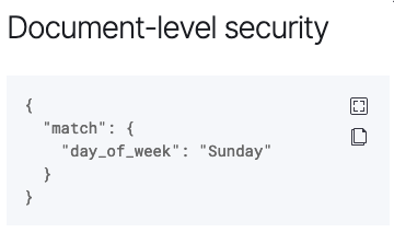
  6. For Document-level security, specify the following query:
    {
      "match": {
        "day_of_week" : "Sunday"
      }
    }

  7. For Field-level security, choose Exclude and specify email.
  8. For Anonymization, specify customer_first_name and customer_full_name.
  9. Choose Create.

You can see the following permissions to the role Orders-placed-on-Sunday.

Choose View expression to see the document-level security.

Map the OpenSearch Service role to the backend role of the Amazon Cognito group

To perform user mapping, complete the following steps:

  1. Go to the OpenSearch Service role Orders-placed-on-Sunday.
  2. Choose Mapped users, Manage mapping.
  3. For Backend roles, enter arn:aws:iam::<account-id>:role/OpenSearchFineGrainedAccessRole.
  4. Choose Map.
  5. Return to the list of roles and choose the predefined role opensearch_dashboards_user, which includes the permissions a user needs to work with index patterns, visualizations, dashboards, and tenants.
  6. Map the opensearch_dashboards_user role to arn:aws:iam::<account-id>:role/OpenSearchFineGrainedAccessRole.

Test the solution

To test your fine-grained access control, complete the following steps:

  1. Log in to the OpenSearch Dashboards URL as ecomuser1.
  2. Go to OpenSearch Plugins and choose Query Workbench.
  3. Run the following SQL queries in OpenSearch Workbench to verify the fine-grained access applied to ecomuser1 as compared to the same queries run by masteruser.
SQL Results when signed-in as masteruser
SHOW tables LIKE %sample%; opensearch_dashboards_sample_data_ecommerce
opensearch_dashboards_sample_data_flights
opensearch_dashboards_sample_data_logs
SELECT COUNT(*) FROM opensearch_dashboards_sample_data_flights ; 13059
SELECT day_of_week, count(*) AS total_records FROM opensearch_dashboards_sample_data_ecommerce GROUP BY day_of_week_i,day_of_week ORDER BY day_of_week_i;
day_of_week total_records
Monday 579
Tuesday 609
Wednesday 592
Thursday 775
Friday 770
Saturday 736
Sunday 614
SELECT customer_last_name AS last_name, customer_full_name AS full_name, email FROM opensearch_dashboards_sample_data_ecommerce WHERE day_of_week = ‘Sunday’ AND order_id = ‘582936’;
last_name full_name email
Miller Gwen Miller [email protected]

..

SQL Results when signed-in as ecomuser1 Observations
SHOW tables LIKE %sample%; no permissions for [indices:admin/get] and User [name=Cognito/<cognito pool-id>/ecomuser1, backend_roles=[arn:aws:iam::<account-id>:role/OpenSearchFineGrainedAccessRole] ecomuser1 can’t list tables.
SELECT COUNT(*) FROM opensearch_dashboards_sample_data_flights ; no permissions for [indices:data/read/search] and User [name=Cognito/<cognito pool-id>/ecomuser1, backend_roles=[arn:aws:iam::<account-id>:role/OpenSearchFineGrainedAccessRole] ecomuser1 can’t see flights data.
SELECT day_of_week, count(*) AS total_records  FROM opensearch_dashboards_sample_data_ecommerce GROUP BY day_of_week_i,day_of_week ORDER BY day_of_week_i;
day_of_week total_records
Sunday 614
ecomuser1 can see ecommerce orders placed on Sunday only.
SELECT customer_last_name AS last_name, customer_full_name AS full_name, email FROM opensearch_dashboards_sample_data_ecommerce WHERE day_of_week = ‘Sunday’ AND order_id = ‘582936’;
last_name full_name email
Miller f1493b0f9039531ed02c9b1b7855707116beca01c6c0d42cf7398b8d880d555f .
For ecomuser1, customer’s email is excluded and customer_full_name is anonymized.

From these results, you can see OpenSearch Service field-level access controls were applied to ecomuser1, restricting the user from seeing the customer’s email. Additionally, the customer’s full name and first name were anonymized when displayed to the user.

Conclusion

When OpenSearch Service fine-grained access control authenticates a user, the request is handled based on the OpenSearch Service roles mapped to the user. This post demonstrated fine-grained access control restricting a user from seeing a customer’s PII data, as per the business requirements.

Role-based fine-grained access control enables you to control access to your data on OpenSearch Service at the index level, document level, and field level. When your logs or applications data has sensitive data, the field-level security permissions can help you provision the right level of access for your users.


About the author

Satya Adimula is a Senior Data Architect at AWS based in Boston. With extensive experience in data and analytics, Satya helps organizations derive their business insights from the data at scale.

Reduce cost and improve query performance with Amazon Athena Query Result Reuse

Post Syndicated from Theo Tolv original https://aws.amazon.com/blogs/big-data/reduce-cost-and-improve-query-performance-with-amazon-athena-query-result-reuse/

Amazon Athena is an interactive query service that makes it easy to analyze data in Amazon Simple Storage Service (Amazon S3) using standard SQL. Athena is serverless, so there is no infrastructure to manage, and you pay only for the queries that you run on datasets at petabyte scale. You can use Athena to query your S3 data lake for use cases such as data exploration for machine learning (ML) and AI, business intelligence (BI) reporting, and ad hoc querying.

It’s not uncommon for datasets in data lakes to update only daily, or at most a few times per day, yet queries running on these datasets may be repeated more frequently. Previously, all queries resulted in a data scan, even if the same query was repeated again. When the source data hasn’t changed, repeat queries run needlessly, leading to the same results with higher data scan costs and query latency. Wouldn’t it be better if the results of a recent query could be reused instead?

Query Result Reuse is a new feature available in Athena engine version 3 that makes it possible to reuse the results of a previous query. This can improve performance and reduce cost for frequently run queries, by skipping scanning the source data and instead returning a previously calculated result directly. With Query Result Reuse, you can tell Athena that you want to reuse results of a previous query run, with a maximum age setting that controls how recent a previous result has to be.

Athena automatically reuses any previous results that match your query and maximum age setting, or transparently runs the query again if no match is found. If you know that a dataset changes a few times per day, you can, for example, tell Athena to reuse results that are up to an hour old to avoid rerunning most queries, but still get new results when you run a query soon after new data has become available.

In this post, we demonstrate how to reduce cost and improve query performance with the new Query Result Reuse feature.

When should you use Query Result Reuse?

We recommend using Query Result Reuse for every query where the source data doesn’t change frequently. You can configure the maximum age of results to reuse per query, or use the default, which is 60 minutes. In certain cases where queries include non-deterministic functions such as RAND(), the query fetches fresh data from the input source even if the Query Result Reuse feature is enabled.

Query Result Reuse allows results to be shared among users in a workgroup, as long as they have access to the tables and data. This means Query Result Reuse can benefit not only a single user, but also other users in the workgroup who might be running the same queries. One example where this may be especially beneficial is when you have dashboards that are viewed by many users. The dashboard widgets run the same queries for all users, and are therefore accelerated by Query Result Reuse, when enabled.

Another example is if you have a dataset that is updated daily, and many users who all query the most recent data to create reports. Different people might run the same queries as part of their work; with Query Result Reuse, they can collectively avoid running the same query more than once, making everyone more productive and lowering overall cost by avoiding repeated scans of the same data.

Finally, if you have a historical dataset that is frequently queried, but never or very rarely updated, you can configure queries to reuse results that are up to 7 days old to maximize the chances of reusing results and avoid unnecessary costs.

How does Query Result Reuse work?

Query Result Reuse takes advantage of the fact that Athena writes query results to Amazon S3 as a CSV file. Before the introduction of Query Result Reuse, it was possible to reuse query results by reading these files directly. You could also use the ClientRequestToken parameter of the StartQueryExecution API to ensure queries are run only once, and subsequent runs return the same results. With Query Result Reuse, the process of reusing query results is easier and more versatile.

When Athena receives a query with Query Result Reuse enabled, it looks for a result for a query with the same query string that was run in the same workgroup. The query string has to be identical in order to match.

Query Result Reuse is enabled on a per query basis. When you run a query, you specify how old a result can be for it to be reused, from 1 minute up to 7 days. If the query has been run before, and a result exists that matches the request, it’s returned, otherwise the query is run and a new result is calculated. This new result is then available to be reused by subsequent queries.

You can run the query multiple times with different settings for how old a result you can accept. Results can be reused within the same workgroup, even if a different user ran the query previously.

Before a query result is reused, Athena does a few checks to make sure that the user is still allowed to see the results. It checks that the user has access to the tables involved in the query and permission to read the result file on Amazon S3.

There are some situations where query results can’t be reused, for example if the query uses non-deterministic functions, or has AWS Lake Form ation fine-grained access controls enabled. These limitations are described in more detail later in this post.

Run queries with Query Result Reuse

In this section, we demonstrate how to run queries with the Query Result Reuse feature via the Athena API, the Athena console, and the JDBC and ODBC drivers.

Run queries using the Athena API

For applications that use the Athena API through the AWS Command Line Interface (AWS CLI) or the AWS SDKs, the StartQueryExecution API call now has the additional parameter ResultReuseConfiguration, where you can enable Query Result Reuse and specify the maximum age of results. For example, when using the AWS CLI, you can run a query with Query Result Reuse enabled as follows:

aws athena start-query-execution \
  --work-group "my_work_group" \
  --query-string "SELECT * FROM my_table LIMIT 10" \
  --result-reuse-configuration \
    "ResultReuseByAgeConfiguration={Enabled=true,MaxAgeInMinutes=60}"

The following code shows how to do this with the AWS SDK for Python:

import boto3

client = boto3.client('athena')
response = client.start_query_execution(
    WorkGroup='my_work_group',
    QueryString='SELECT * FROM my_table LIMIT 10',
    ResultReuseConfiguration={
        'ResultReuseByAgeConfiguration': {
   	    	'Enabled': True,
     		'MaxAgeInSeconds': 60
        }
    }
)

These examples assume that my_work_group uses Athena engine v3, that the workgroup has an output location configured, and that the AWS Region has been set in the AWS CLI configuration.

When a query result is reused, you can see in the statistics section of the response from the GetQueryExecution API call that no data was scanned and that results were reused:

{
    "QueryExecution": {
        …
        "Statistics": {
            "EngineExecutionTimeInMillis": 272,
            "DataScannedInBytes": 0,
            "TotalExecutionTimeInMillis": 445,
            "QueryQueueTimeInMillis": 143,
            "ServiceProcessingTimeInMillis": 30,
            "ResultReuseInformation": {
               	"ReusedPreviousResult": true
           	}
        }
    }
}

Run queries using the Athena console

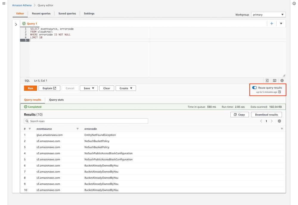
When you run queries on the Athena console, Query Result Reuse is now enabled by default. You can enable and disable Query Result Reuse in the query editor. You can also choose the pen icon to change the maximum age of results. This setting applies to all queries run on the Athena console.

The following screenshot shows an example query run against AWS CloudTrail logs with Query Result Reuse enabled.

When we ran the query again, the results showed up immediately, and we could see the message “using reused query results” in the Query results pane as a confirmation that the results of our first query had been reused. The Data scanned statistic also showed “-” to indicate that no data was scanned.

Run queries using the JDBC and ODBC drivers

If you use the JDBC or ODBC driver to query Athena, you can now add enableResultReuse=1 to your connection parameters to enable Query Result Reuse, and use ageforResultReuse=60 to set the maximum age to 60 minutes. The drivers automatically apply the setting to all queries running in the context of the connection.

For more information on how to connect to Athena via JDBC and ODBC, refer to Connecting to Amazon Athena with ODBC and JDBC drivers.

Limitations and considerations

Query Result Reuse is supported for most Athena queries, but there are some limitations. We want to ensure that reusing results doesn’t create surprising situations, or expose results that a user shouldn’t have access to. For that reason, Athena always runs a fresh query in the following situations:

  • Non-deterministic functions – Some functions and expressions produce different results from query to query, such as CURRENT_TIME and RAND(). Results for queries that use temporal and non-deterministic expressions and functions aren’t reusable because that could create surprising and inconsistent results.
  • Fine-grained access controls – Row-level and column-level permissions are configured in Lake Formation, and Athena can’t know if these have changed since a previous query result was created. Users using the same workgroup can also have different permissions, and checking all permissions would undo many of the cost and performance savings you get from Query Result Reuse.
  • Federated queries, user-defined functions (UDFs), and external Hive metastores – Users using the same workgroup can have different permissions to invoke the AWS Lambda functions that these features rely on. Athena isn’t able to check that a user that wants to reuse a result has permission to invoke these Lambda functions without running the query, which would negate the cost and performance savings.

Athena detects these conditions automatically and runs the query as if Query Result Reuse wasn’t enabled. You won’t get errors, but you can determine that Query Result Reuse wasn’t in effect by inspecting the query status (see our earlier examples).

Query Result Reuse is available in Athena engine version 3 only.

Conclusion

Query Result Reuse is a new feature in Athena that aims to reduce cost and query response times for datasets that change less frequently than they are queried. For teams that often run the same query, or have dashboards that are used more often than the data changes, Query Result Reuse can result in lower costs and faster results. It’s easy to get started with Query Result Reuse via the Athena console, API, and JDBC/ODBC; all you have to do is set the maximum age of results, and run your queries as usual.

We hope that you will like this new feature, and that it will save cost and improve performance for you and your team!


About the authors

Theo Tolv is a Senior Big Data Architect in the Athena team. He’s worked with small and big data for most of his career and often hangs out on Stack Overflow answering questions about Athena.

Vijay Jain is a Senior Product Manager in Amazon Web Services (AWS) Athena team. He is passionate about building scalable analytics technologies and products working closely with enterprise customers. Outside of work, Vijay likes running and spending time with his family.

What’s new with Amazon QuickSight at AWS re:Invent 2022

Post Syndicated from Mia Heard original https://aws.amazon.com/blogs/big-data/whats-new-with-amazon-quicksight-at-aws-reinvent-2022/

AWS re:Invent is a learning conference hosted by AWS for the global cloud computing community. This year’s re:Invent will be held in Las Vegas, Nevada, from November 28 to December 2.

Amazon QuickSight is the most popular cloud-native serverless BI service. This post walks you through the details of all QuickSight-related sessions and activities to help you plan your conference week accordingly. These sessions should appeal to data and analytics teams, product and engineering teams, and line of business and technology leaders interested in modernizing their BI capabilities to transform data into actionable insights for all.

To access the session catalog and reserve your seat for one of our BI sessions, you must be registered for re:Invent. Register now!

Keynotes

Adam Selipsky, Chief Executive Officer of Amazon Web Services – Keynote

Tuesday November 29 | 8:30 AM – 10:30 AM PST | The Venetian

Join Adam Selipsky, Chief Executive Officer of Amazon Web Services, as he looks at the ways that forward-thinking builders are transforming industries and even our future, powered by AWS. He highlights innovations in data, infrastructure, and more that are helping customers achieve their goals faster, take advantage of untapped potential, and create a better future with AWS.

Swami Sivasubramanian, Vice President of AWS Data and Machine Learning – Keynote

Wednesday November 30 | 8:30 AM – 10:30 AM PST | The Venetian

Join Swami Sivasubramanian, Vice President of AWS Data and Machine Learning, as he reveals the latest AWS innovations that can help you transform your company’s data into meaningful insights and actions for your business. In this keynote, several speakers discuss the key components of a future-proof data strategy and how to empower your organization to drive the next wave of modern invention with data. Hear from leading AWS customers who are using data to bring new experiences to life for their customers.

Leadership sessions

ANT203-L (LVL 200) Unlock the value of your data with AWS analytics

Wednesday November 30 | 2:30 – 3:30 PM PST | The Venetian

Data fuels digital transformation and drives effective business decisions. To survive in an ever-changing world, organizations are turning to data to derive insights, create new experiences, and reinvent themselves so they can remain relevant today and in the future. AWS offers analytics services that allow organizations to gain faster and deeper insights from all their data. In this session, G2 Krishnamoorthy, VP of AWS Analytics, addresses the current state of analytics on AWS, covers the latest service innovations around data, and highlights customer successes with AWS analytics. Also, learn from organizations like FINRA and more who have turned to AWS for their digital transformation journey.
Reserve your seat now!

BSI201 (LVL 200) Reinvent how you derive value from your data with Amazon QuickSight

Tuesday November 29 | 2:00 PM – 3:00 PM PST | Mandalay Bay

In this session, learn how you can use AWS-native business analytics to provide your users with machine learning-powered interactive dashboards, natural language query (NLQ), and embedded analytics to provide insights to users at scale, when and where they need it. Join this session to also learn more about how Amazon uses QuickSight internally.
Reserve your seat now!

Breakout sessions

BSI202 (LVL 200) Migrate to cloud-native business analytics with Amazon QuickSight

Wednesday November 30 | 2:30 PM – 3:30 PM PST | Encore

Legacy BI systems can hurt agile decision-making in the modern organization, with expensive licensing, outdated capabilities, and expensive infrastructure management. In this session, discover how migrating your BI to the cloud with cloud-native, fully managed business analytics capabilities from QuickSight can help you overcome these challenges. Learn how you can use QuickSight’s interactive dashboards and reporting capabilities to provide insights to every user in the organization, lowering your costs and enabling better decision-making. Join this session to also learn more about Siemens QuickSight use case.
Reserve your seat now!

BSI207 (LVL 200) Get clarity on your data in seconds with Amazon QuickSight Q

Wednesday November 30 | 4:45 PM – 5:45 PM PST | MGM Grand

Amazon QuickSight Q is a machine learning–powered natural language capability that empowers business users to ask questions about all of their data using everyday business language and get answers in seconds. Q interprets questions to understand their intent and generates an answer instantly in the form of a visual without requiring authors to create graphics, dashboards, or analyses. In this session, the QuickSight Q team provides an overview and demonstration of Q in action. Join this session to also learn more about NASDAQ’s QuickSight use case.
Reserve your seat now!

BSI203 (LVL 200) Differentiate your apps with Amazon QuickSight embedded analytics

Thursday December 1 | 12:30 PM – 1:30 PM PST | Caesars Forum

In this session, learn how to enable new monetization opportunities and grow your business with QuickSight embedded analytics. Discover how you can differentiate your end-user experience by embedding data visualizations, dashboards, and ML-powered natural language query into your applications at scale with no infrastructure to manage. Join this session to also learn more about Guardian Life and Showpad’s QuickSight use case.
Reserve your seat now!

BSI304 (LVL 300) Optimize your AWS cost and usage with Cloud Intelligence Dashboards

Thursday December 1 | 3:30 PM – 4:30 PM PST | Encore

Do your engineers know how much they’re spending? Do you have insight into the details of your cost and usage on AWS? Are you taking advantage of all your cost optimization opportunities? Attend this session to learn how organizations are using the Cloud Intelligence Dashboards to start their FinOps journeys and create cost-aware cultures within their organizations. Dive deep into specific use cases and learn how you can use these insights to drive and measure your cost optimization efforts. Discover how unit economics, resource-level visibility, and periodic spend updates make it possible for FinOps practitioners, developers, and business executives to come together to make smarter decisions. Join this session to also learn more about Dolby laboratories’ QuickSight use case.
Reserve your seat now!

Chalk talks

BSI302 (LVL 300) Deploy your BI assets at scale to thousands with Amazon QuickSight

Tuesday November 29 | 11:45 AM – 12:45 AM PST | Wynn
As your user bases grow to hundreds or thousands of users, managing assets and user permissions at scale becomes increasingly important. In this chalk talk, learn about best practices for content development, promotion, authorization, organization, and cleanup to help ensure that your users are developing and sharing content in a safe and scalable manner.
Reserve your seat now!

BSI301 (LVL 300) Architecting multi-tenancy for your apps with Amazon QuickSight

Tuesday November 29 | 2:45 PM – 3:45 PM PST | Caesars Forum

Whether you are deploying QuickSight internally in a centrally managed single account or developing a SaaS application with multiple external tenants, it is paramount to focus on security and governance and to isolate tenants from each other. In this chalk talk, learn about different architectures and security frameworks that you can use to deploy QuickSight to thousands of departments or clients in a scalable and controlled manner.
Reserve your seat now!

*This session will also be repeated Wednesday November 30 | 7:45 PM – 8:45 PM PST | Wynn

BSI401 (LVL 400) Insightful dashboards through advanced calculations with QuickSight

Monday November 28 | 12:15 PM – 1:15 PM PST | MGM Grand
Loading data into various charting types is very rarely the end goal for your users. When they find interesting patterns or trends, they tend to dig deeper into their data and use calculations to surface more underlying insights. In this chalk talk, learn about various ways to build insightful and creative dashboards using QuickSight’s new advanced calculation capabilities, such as level-aware calculation and period functions.
Reserve your seat now!

Workshops

BSI205 (LVL 200) Build stunning customized dashboards with Amazon QuickSight

Monday November 28 | 10:45 AM – 12:45 PM PST | Wynn

Want to grow your dashboard building skills? In this workshop, the QuickSight team demonstrates the latest authoring functionality designed to empower you to build beautiful layouts and robust interactive experiences with other applications, right from within your dashboard. You must bring your laptop to participate.
Reserve your seat now!

*This session will be also be repeated Thursday December 1 | 11:45 AM – 1:45 PM PST | Caesars Forum

BSI303 (LVL 300) Seamlessly embed analytics into your apps with Amazon QuickSight
Wednesday November 30 | 5:30 PM – 7:30 PM PST | Wynn

In this workshop, learn how you can bring data insights to your internal teams and end customers by simply and seamlessly embedding rich, interactive data visualizations and dashboards into your web applications and portals. You must bring your laptop to participate.
Reserve your seat now!

Partner session

PEX307 (LVL 300) Migrating business intelligence systems to Amazon QuickSight

Wednesday November 30 | 9:15 AM – 10:15 AM PST | Encore

QuickSight is a scalable, serverless, embeddable, machine learning–powered BI tool built for the cloud. If you’re building a cloud-native BI solution and are unsure how to migrate on AWS, this session is for you. Dive deep into BI best practices, tools, and methodologies for migrating BI dashboards to QuickSight, and learn how to use APIs and the AWS CLI to automate common migration tasks required to perform BI dashboard migration. This session is intended for AWS Partners.
Reserve your seat now!

Additional activities

Business Intelligence kiosk in the AWS Village

Visit the Business Intelligence kiosk within the AWS Village to meet with experts to dive deeper into QuickSight capabilities such as Q and embedded analytics. You will be able to ask our experts questions and experience live demos for our newly launched capabilities.

Free QuickSight swag

Make sure to stop by the swag distribution table to grab free QuickSight swag if you have attended either the Business Intelligence kiosk or one of our breakout sessions, chalk talks, or workshops.

Useful resources

Whether you plan on attending re:Invent in person or view available content virtually, you can always learn more about QuickSight through these helpful resources:

QuickSight Community Hub – Ask, answer, and learn with others in the QuickSight Community.

QuickSight YouTube channel – Subscribe to stay up to date on the latest QuickSight workshops, how tos, and demo videos.

QuickSight DemoCentral – Experience QuickSight first-hand through interactive dashboards and demos


About the authors

Mia Heard is a Product Marketing Manager for Amazon QuickSight, AWS’ cloud-native, fully managed BI service.

California State University Chancellor’s Office reduces cost and improves efficiency using Amazon QuickSight for streamlined HR reporting in higher education

Post Syndicated from Madi Hsieh original https://aws.amazon.com/blogs/big-data/california-state-university-chancellors-office-reduces-cost-and-improves-efficiency-using-amazon-quicksight-for-streamlined-hr-reporting-in-higher-education/

The California State University Chancellor’s Office (CSUCO) sits at the center of America’s most significant and diverse 4-year universities. The California State University (CSU) serves approximately 477,000 students and employs more than 55,000 staff and faculty members across 23 universities and 7 off-campus centers. The CSU provides students with opportunities to develop intellectually and personally, and to contribute back to the communities throughout California. For this large organization, managing a wide system of campuses while maintaining the decentralized autonomy of each is crucial. In 2019, they needed a highly secure tool to streamline the process of pulling HR data. The CSU had been using a legacy central data warehouse based on data from their financial system, but it lacked the robustness to keep up with modern technology. This wasn’t going to work for their HR reporting needs.

Looking for a tool to match the cloud-based infrastructure of their other operations, the Business Intelligence and Data Operations (BI/DO) team within the Chancellor’s Office chose Amazon QuickSight, a fast, easy-to-use, cloud-powered business analytics service that makes it easy for all employees within an organization to build visualizations, perform ad hoc analysis, and quickly get business insights from their data, any time, on any device. The team uses QuickSight to organize HR information across the CSU, implementing a centralized security system.

“It’s easy to use, very straightforward, and relatively intuitive. When you couple the experience of using QuickSight, with a huge cost difference to [the BI platform we had been using], to me, it’s a simple choice,”

– Andy Sydnor, Director Business Intelligence and Data Operations at the CSUCO.

With QuickSight, the team has the capability to harness security measures and deliver data insights efficiently across their campuses.

In this post, we share how the CSUCO uses QuickSight to reduce cost and improve efficiency in their HR reporting.

Delivering BI insights across the CSU’s 23 universities

The CSUCO serves the university system’s faculty, students, and staff by overseeing operations in several areas, including finance, HR, student information, and space and facilities. Since migrating to QuickSight in 2019, the team has built dashboards to support these operations. Dashboards include COVID-related leaves of absence, historical financial reports, and employee training data, along with a large selection of dashboards to track employee data at an individual campus level or from a system-wide perspective.

The team created a process for reading security roles from the ERP system and then translating them using QuickSight groups for internal HR reporting. QuickSight allowed them to match security measures with the benefits of low maintenance and familiarity to their end-users.

With QuickSight, the CSUCO is able to run a decentralized security process where campus security teams can provision access directly and users can get to their data faster. Before transitioning to QuickSight, the BI/DO team spent hours trying to get to specific individual-level data, but with QuickSight, the retrieval time was shortened to just minutes. For the first time, Sydnor and his team were able to pinpoint a specific employee’s work history without having to take additional actions to find the exact data they needed.

Cost savings compared to other BI tools

Sydnor shares that, for a public organization, one of the most attractive qualities of QuickSight is the immense cost savings. The BI/DO team at the Chancellor’s Office estimates that they’re saving roughly 40% on costs since switching from their previous BI platform, which is a huge benefit for a public organization of this scale. Their previous BI tool was costing them extensive amounts of money on licensing for features they didn’t require; the CSUCO felt they weren’t getting the best use of their investment.

The functionality of QuickSight to meet their reporting needs at an affordable price point is what makes QuickSight the CSUCO’s preferred BI reporting tool. Sydnor likes that with QuickSight, “we don’t have to go out and buy a subscription or a license for somebody, we can just provision access. It’s much easier to distribute the product.” QuickSight allows the CSUCO to focus their budget in other areas rather than having to pay for charges by infrequent users.

Simple and intuitive interface

Getting started in QuickSight was a no-brainer for Sydnor and his team. As a public organization, the procurement process can be cumbersome, thereby slowing down valuable time for putting their data to action. As an existing AWS customer, the CSUCO could seamlessly integrate QuickSight into their package of AWS services. An issue they were running into with other BI tools was encountering roadblocks to setting up the system, which wasn’t an issue with QuickSight, because it’s a fully managed service that doesn’t require deploying any servers.

The following screenshot shows an example of the CSUCO security audit dashboard.

example of the CSUCO security audit dashboard.

Sydnor tells us, “Our previous BI tool had a huge library of visualization, but we don’t need 95% of those. Our presentations look great with the breadth of visuals QuickSight provides. Most people just want the data and ultimately, need a robust vehicle to get data out of a database and onto a table or visualization.”

Converting from their original BI tool to QuickSight was painless for his team. Sydnor tells us that he has “yet to see something we can’t do with QuickSight.” One of Sydnor’s employees who was a user of the previous tool learned QuickSight in just 30 minutes. Now, they conduct QuickSight demos all the time.

Looking to the future: Expanding BI integration and adopting Amazon QuickSight Q

With QuickSight, the Chancellor’s Office aims to roll out more HR dashboards across its campuses and extend the tool for faculty use in the classroom. In the upcoming year, two campuses are joining CSUCO in building their own HR reporting dashboards through QuickSight. The organization is also making plans to use QuickSight to report on student data and implement external-facing dashboards. Some of the data points they’re excited to explore are insights into at-risk students and classroom scheduling on campus.

Thinking ahead, CSUCO is considering Amazon QuickSight Q, a machine learning-powered natural language capability that gives anyone in an organization the ability to ask business questions in natural language and receive accurate answers with relevant visualizations. Sydnor says, “How cool would that be if professors could go in and ask simple, straightforward questions like, ‘How many of my department’s students are taking full course loads this semester?’ It has a lot of potential.”

Summary

The CSUCO is excited to be a champion of QuickSight in the CSU, and are looking for ways to increase its implementation across their organization in the future.

To learn more, visit the website for the California State University Chancellor’s Office. For more on QuickSight, visit the Amazon QuickSight product page, or browse other Big Data Blog posts featuring QuickSight.


About the authors

Madi Hsieh, AWS 2022 Summer Intern, UCLA.

Tina Kelleher, Program Manager at AWS.

Build the next generation, cross-account, event-driven data pipeline orchestration product

Post Syndicated from Maria Guerra original https://aws.amazon.com/blogs/big-data/build-the-next-generation-cross-account-event-driven-data-pipeline-orchestration-product/

This is a guest post by Mehdi Bendriss, Mohamad Shaker, and Arvid Reiche from Scout24.

At Scout24 SE, we love data pipelines, with over 700 pipelines running daily in production, spread across over 100 AWS accounts. As we democratize data and our data platform tooling, each team can create, maintain, and run their own data pipelines in their own AWS account. This freedom and flexibility is required to build scalable organizations. However, it’s full of pitfalls. With no rules in place, chaos is inevitable.

We took a long road to get here. We’ve been developing our own custom data platform since 2015, developing most tools ourselves. Since 2016, we have our self-developed legacy data pipeline orchestration tool.

The motivation to invest a year of work into a new solution was driven by two factors:

  • Lack of transparency on data lineage, especially dependency and availability of data
  • Little room to implement governance

As a technical platform, our target user base for our tooling includes data engineers, data analysts, data scientists, and software engineers. We share the vision that anyone with relevant business context and minimal technical skills can create, deploy, and maintain a data pipeline.

In this context, in 2015 we created the predecessor of our new tool, which allows users to describe their pipeline in a YAML file as a list of steps. It worked well for a while, but we faced many problems along the way, notably:

  • Our product didn’t support pipelines to be triggered by the status of other pipelines, but based on the presence of _SUCCESS files in Amazon Simple Storage Service (Amazon S3). Here we relied on periodic pulls. In complex organizations, data jobs often have strong dependencies to other work streams.
  • Given the previous point, most pipelines could only be scheduled based on a rough estimate of when their parent pipelines might finish. This led to cascaded failures when the parents failed or didn’t finish on time.
  • When a pipeline fails and gets fixed, then manually redeployed, all its dependent pipelines must be rerun manually. This means that the data producer bears the responsibility of notifying every single team downstream.

Having data and tooling democratized without the ability to provide insights into which jobs, data, and dependencies exist diminishes synergies within the company, leading to silos and problems in resource allocation. It became clear that we needed a successor for this product that would give more flexibility to the end-user, less computing costs, and no infrastructure management overhead.

In this post, we describe, through a hypothetical case study, the constraints under which the new solution should perform, the end-user experience, and the detailed architecture of the solution.

Case study

Our case study looks at the following teams:

  • The core-data-availability team has a data pipeline named listings that runs every day at 3:00 AM on the AWS account Account A, and produces on Amazon S3 an aggregate of the listings events published on the platform on the previous day.
  • The search team has a data pipeline named searches that runs every day at 5:00 AM on the AWS account Account B, and exports to Amazon S3 the list of search events that happened on the previous day.
  • The rent-journey team wants to measure a metric referred to as X; they create a pipeline named pipeline-X that runs daily on the AWS account Account C, and relies on the data of both previous pipelines. pipeline-X should only run daily, and only after both the listings and searches pipelines succeed.

User experience

We provide users with a CLI tool that we call DataMario (relating to its predecessor DataWario), and which allows users to do the following:

  • Set up their AWS account with the necessary infrastructure needed to run our solution
  • Bootstrap and manage their data pipeline projects (creating, deploying, deleting, and so on)

When creating a new project with the CLI, we generate (and require) every project to have a pipeline.yaml file. This file describes the pipeline steps and the way they should be triggered, alerting, type of instances and clusters in which the pipeline will be running, and more.

In addition to the pipeline.yaml file, we allow advanced users with very niche and custom needs to create their pipeline definition entirely using a TypeScript API we provide them, which allows them to use the whole collection of constructs in the AWS Cloud Development Kit (AWS CDK) library.

For the sake of simplicity, we focus on the triggering of pipelines and the alerting in this post, along with the definition of pipelines through pipeline.yaml.

The listings and searches pipelines are triggered as per a scheduling rule, which the team defines in the pipeline.yaml file as follows:

trigger: 
    schedule: 
        hour: 3

pipeline-x is triggered depending on the success of both the listings and searches pipelines. The team defines this dependency relationship in the project’s pipeline.yaml file as follows:

trigger: 
    executions: 
        allOf: 
            - name: listings 
              account: Account_A_ID 
              status: 
                  - SUCCESS 
            - name: searches 
              account: Account_B_ID 
              status: 
                  - SUCCESS

The executions block can define a complex set of relationships by combining the allOf and anyOf blocks, along with a logical operator operator: OR / AND, which allows mixing the allOf and anyOf blocks. We focus on the most basic use case in this post.

Accounts setup

To support alerting, logging, and dependencies management, our solution has components that must be pre-deployed in two types of accounts:

  • A central AWS account – This is managed by the Data Platform team and contains the following:
    • A central data pipeline Amazon EventBridge bus receiving all the run status changes of AWS Step Functions workflows running in user accounts
    • An AWS Lambda function logging the Step Functions workflow run changes in an Amazon DynamoDB table to verify if any downstream pipelines should be triggered based on the current event and previous run status changes log
    • A Slack alerting service to send alerts to the Slack channels specified by users
    • A trigger management service that broadcasts triggering events to the downstream buses in the user accounts
  • All AWS user accounts using the service – These accounts contain the following:
    • A data pipeline EventBridge bus that receives Step Functions workflow run status changes forwarded from the central EventBridge bus
    • An S3 bucket to store data pipelines artifacts, along their logs
    • Resources needed to run Amazon EMR clusters, like security groups, AWS Identity and Access Management (IAM) roles, and more

With the provided CLI, users can set up their account by running the following code:

$ dpc setup-user-account

Solution overview

The following diagram illustrates the architecture of the cross-account, event-driven pipeline orchestration product.

In this post, we refer to the different colored and numbered squares to reference a component in the architecture diagram. For example, the green square with label 3 refers to the EventBridge bus default component.

Deployment flow

This section is illustrated with the orange squares in the architecture diagram.

A user can create a project consisting of a data pipeline or more using our CLI tool as follows:

$ dpc create-project -n 'project-name'

The created project contains several components that allow the user to create and deploy data pipelines, which are defined in .yaml files (as explained earlier in the User experience section).

The workflow of deploying a data pipeline such as listings in Account A is as follows:

  • Deploy listings by running the command dpc deploy in the root folder of the project. An AWS CDK stack with all required resources is automatically generated.
  • The previous stack is deployed as an AWS CloudFormation template.
  • The stack uses custom resources to perform some actions, such as storing information needed for alerting and pipeline dependency management.
  • Two Lambda functions are triggered, one to store the mapping pipeline-X/slack-channels used for alerting in a DynamoDB table, and another one to store the mapping between the deployed pipeline and its triggers (other pipelines that should result in triggering the current one).
  • To decouple alerting and dependency management services from the other components of the solution, we use Amazon API Gateway for two components:
    • The Slack API.
    • The dependency management API.
  • All calls for both APIs are traced in Amazon CloudWatch log groups and two Lambda functions:
    • The Slack channel publisher Lambda function, used to store the mapping pipeline_name/slack_channels in a DynamoDB table.
    • The dependencies publisher Lambda function, used to store the pipelines dependencies (the mapping pipeline_name/parents) in a DynamoDB table.

Pipeline trigger flow

This is an event-driven mechanism that ensures that data pipelines are triggered as requested by the user, either following a schedule or a list of fulfilled upstream conditions, such as a group of pipelines succeeding or failing.

This flow relies heavily on EventBridge buses and rules, specifically two types of rules:

  • Scheduling rules.
  • Step Functions event-based rules, with a payload matching the set of statuses of all the parents of a given pipeline. The rules indicate for which set of statuses all the parents of pipeline-X should be triggered.

Scheduling

This section is illustrated with the black squares in the architecture diagram.

The listings pipeline running on Account A is set to run every day at 3:00 AM. The deployment of this pipeline creates an EventBridge rule and a Step Functions workflow for running the pipeline:

  • The EventBridge rule is of type schedule and is created on the default bus (this is the EventBridge bus responsible for listening to native AWS events—this distinction is important to avoid confusion when introducing the other buses). This rule has two main components:
    • A cron-like notation to describe the frequency at which it runs: 0 3 * * ? *.
    • The target, which is the Step Functions workflow describing the workflow of the listings pipeline.
  • The listings Step Function workflow describes and runs immediately when the rule gets triggered. (The same happens to the searches pipeline.)

Each user account has a default EventBridge bus, which listens to the default AWS events (such as the run of any Lambda function) and scheduled rules.

Dependency management

This section is illustrated with the green squares in the architecture diagram. The current flow starts after the Step Functions workflow (black square 2) starts, as explained in the previous section.

As a reminder, pipeline-X is triggered when both the listings and searches pipelines are successful. We focus on the listings pipeline for this post, but the same applies to the searches pipeline.

The overall idea is to notify all downstream pipelines that depend on it, in every AWS account, passing by and going through the central orchestration account, of the change of status of the listings pipeline.

It’s then logical that the following flow gets triggered multiple times per pipeline (Step Functions workflow) run as its status changes from RUNNING to either SUCCEEDED, FAILED, TIMED_OUT, or ABORTED. The reason being that there could be pipelines downstream potentially listening on any of those status change events. The steps are as follows:

  • The event of the Step Functions workflow starting is listened to by the default bus of Account A.
  • The rule export-events-to-central-bus, which specifically listens to the Step Function workflow run status change events, is then triggered.
  • The rule forwards the event to the central bus on the central account.
  • The event is then caught by the rule trigger-events-manager.
  • This rule triggers a Lambda function.
  • The function gets the list of all children pipelines that depend on the current run status of listings.
  • The current run is inserted in the run log Amazon Relational Database Service (Amazon RDS) table, following the schema sfn-listings, time (timestamp), status (SUCCEEDED, FAILED, and so on). You can query the run log RDS table to evaluate the running preconditions of all children pipelines and get all those that qualify for triggering.
  • A triggering event is broadcast in the central bus for each of those eligible children.
  • Those events get broadcast to all accounts through the export rules—including Account C, which is of interest in our case.
  • The default EventBridge bus on Account C receives the broadcasted event.
  • The EventBridge rule gets triggered if the event content matches the expected payload of the rule (notably that both pipelines have a SUCCEEDED status).
  • If the payload is valid, the rule triggers the Step Functions workflow pipeline-X and triggers the workflow to provision resources (which we discuss later in this post).

Alerting

This section is illustrated with the gray squares in the architecture diagram.

Many teams handle alerting differently across the organization, such as Slack alerting messages, email alerts, and OpsGenie alerts.

We decided to allow users to choose their preferred methods of alerting, giving them the flexibility to choose what kind of alerts to receive:

  • At the step level – Tracking the entire run of the pipeline
  • At the pipeline level – When it fails, or when it finishes with a SUCCESS or FAILED status

During the deployment of the pipeline, a new Amazon Simple Notification Service (Amazon SNS) topic gets created with the subscriptions matching the targets specified by the user (URL for OpsGenie, Lambda for Slack or email).

The following code is an example of what it looks like in the user’s pipeline.yaml:

notifications:
    type: FULL_EXECUTION
    targets:
        - channel: SLACK
          addresses:
               - data-pipeline-alerts
        - channel: EMAIL
          addresses:
               - [email protected]

The alerting flow includes the following steps:

  1. As the pipeline (Step Functions workflow) starts (black square 2 in the diagram), the run gets logged into CloudWatch Logs in a log group corresponding to the name of the pipeline (for example, listings).
  2. Depending on the user preference, all the run steps or events may get logged or not thanks to a subscription filter whose target is the execution-tracker-lambda Lambda function. The function gets called anytime a new event gets published in CloudWatch.
  3. This Lambda function parses and formats the message, then publishes it to the SNS topic.
  4. For the email and OpsGenie flows, the flow stops here. For posting the alert message on Slack, the Slack API caller Lambda function gets called with the formatted event payload.
  5. The function then publishes the message to the /messages endpoint of the Slack API Gateway.
  6. The Lambda function behind this endpoint runs, and posts the message in the corresponding Slack channel and under the right Slack thread (if applicable).
  7. The function retrieves the secret Slack REST API key from AWS Secrets Manager.
  8. It retrieves the Slack channels in which the alert should be posted.
  9. It retrieves the root message of the run, if any, so that subsequent messages get posted under the current run thread on Slack.
  10. It posts the message on Slack.
  11. If this is the first message for this run, it stores the mapping with the DB schema execution/slack_message_id to initiate a thread for future messages related to the same run.

Resource provisioning

This section is illustrated with the light blue squares in the architecture diagram.

To run a data pipeline, we need to provision an EMR cluster, which in turn requires some information like Hive metastore credentials, as shown in the workflow. The workflow steps are as follows:

  • Trigger the Step Functions workflow listings on schedule.
  • Run the listings workflow.
  • Provision an EMR cluster.
  • Use a custom resource to decrypt the Hive metastore password to be used in Spark jobs relying on central Hive tables or views.

End-user experience

After all preconditions are fulfilled (both the listings and searches pipelines succeeded), the pipeline-X workflow runs as shown in the following diagram.

As shown in the diagram, the pipeline description (as a sequence of steps) defined by the user in the pipeline.yaml is represented by the orange block.

The steps before and after this orange section are automatically generated by our product, so users don’t have to take care of provisioning and freeing compute resources. In short, the CLI tool we provide our users synthesizes the user’s pipeline definition in the pipeline.yaml and generates the corresponding DAG.

Additional considerations and next steps

We tried to stay consistent and stick to one programming language for the creation of this product. We chose TypeScript, which played well with AWS CDK, the infrastructure as code (IaC) framework that we used to build the infrastructure of the product.

Similarly, we chose TypeScript for building the business logic of our Lambda functions, and of the CLI tool (using Oclif) we provide for our users.

As demonstrated in this post, EventBridge is a powerful service for event-driven architectures, and it plays a central and important role in our products. As for its limitations, we found that pairing Lambda and EventBridge could fulfill all our current needs and granted a high level of customization that allowed us to be creative in the features we wanted to serve our users.

Needless to say, we plan to keep developing the product, and have a multitude of ideas, notably:

  • Extend the list of core resources on which workloads run (currently only Amazon EMR) by adding other compute services, such Amazon Elastic Compute Cloud (Amazon EC2)
  • Use the Constructs Hub to allow users in the organization to develop custom steps to be used in all data pipelines (we currently only offer Spark and shell steps, which suffice in most cases)
  • Use the stored metadata regarding pipeline dependencies for data lineage, to have an overview of the overall health of the data pipelines in the organization, and more

Conclusion

This architecture and product brought many benefits. It allows us to:

  • Have a more robust and clear dependency management of data pipelines at Scout24.
  • Save on compute costs by avoiding scheduling pipelines based approximately on when its predecessors are usually triggered. By shifting to an event-driven paradigm, no pipeline gets started unless all its prerequisites are fulfilled.
  • Track our pipelines granularly and in real time on a step level.
  • Provide more flexible and alternative business logic by exposing multiple event types that downstream pipelines can listen to. For example, a fallback downstream pipeline might be run in case of a parent pipeline failure.
  • Reduce the cross-team communication overhead in case of failures or stopped runs by increasing the transparency of the whole pipelines’ dependency landscape.
  • Avoid manually restarting pipelines after an upstream pipeline is fixed.
  • Have an overview of all jobs that run.
  • Support the creation of a performance culture characterized by accountability.

We have big plans for this product. We will use DataMario to implement granular data lineage, observability, and governance. It’s a key piece of infrastructure in our strategy to scale data engineering and analytics at Scout24.

We will make DataMario open source towards the end of 2022. This is in line with our strategy to promote our approach to a solution on a self-built, scalable data platform. And with our next steps, we hope to extend this list of benefits and ease the pain in other companies solving similar challenges.

Thank you for reading.


About the authors

Mehdi Bendriss is a Senior Data / Data Platform Engineer, MSc in Computer Science and over 9 years of experience in software, ML, and data and data platform engineering, designing and building large-scale data and data platform products.

Mohamad Shaker is a Senior Data / Data Platform Engineer, with over 9 years of experience in software and data engineering, designing and building large-scale data and data platform products that enable users to access, explore, and utilize their data to build great data products.

Arvid Reiche is a Data Platform Leader, with over 9 years of experience in data, building a data platform that scales and serves the needs of the users.

Marco Salazar is a Solutions Architect working with Digital Native customers in the DACH region with over 5 years of experience building and delivering end-to-end, high-impact, cloud native solutions on AWS for Enterprise and Sports customers across EMEA. He currently focuses on enabling customers to define technology strategies on AWS for the short- and long-term that allow them achieve their desired business objectives, specializing on Data and Analytics engagements. In his free time, Marco enjoys building side-projects involving mobile/web apps, microcontrollers & IoT, and most recently wearable technologies.

Your guide to AWS Analytics at re:Invent 2022

Post Syndicated from Imtiaz Sayed original https://aws.amazon.com/blogs/big-data/your-guide-to-aws-analytics-at-reinvent-2022/

Join the global cloud community at AWS re:Invent this year to meet, get inspired, and rethink what’s possible!

Reserved seating is available for registered attendees to secure seats in the sessions of their choice. You can reserve a seat in your favorite sessions by signing in to the attendee portal and navigating to Event > Sessions. For those who can’t make it in person, you can get your free online pass to watch live keynotes and leadership sessions by registering for a virtual-only access. This curated attendee guide helps data and analytics enthusiasts manage their schedule*, as well as navigate the AWS analytics and business intelligence tracks to get the best out of re:Invent.

For additional session details, visit the AWS Analytics splash page.

#AWSanalytics, #awsfordata, #reinvent22

Keynotes

KEY002 | Adam Selipsky (CEO, Amazon Web Services) | Tuesday, November 29 | 8:30 AM – 10:30 AM

Join Adam Selipsky, CEO of Amazon Web Services, as he looks at the ways that forward-thinking builders are transforming industries and even our future, powered by AWS.

KEY003 | Swami Sivasubramanian (Vice President, AWS Data and Machine Learning) | Wednesday, November 30 | 8:30 AM – 10:30 AM

Join Swami Sivasubramanian, Vice President of AWS Data and Machine Learning, as he reveals the latest AWS innovations that can help you transform your company’s data into meaningful insights and actions for your business.

Leadership sessions

ANT203-L | Unlock the value of your data with AWS analytics | G2 Krishnamoorthy, VP of AWS Analytics | Wednesday, November 30 | 2:30 PM – 3:30 PM

G2 addresses the current state of analytics on AWS, covers the latest service innovations around data, and highlights customer successes with AWS analytics. Also, learn from organizations like FINRA and more who have turned to AWS for their digital transformation journey.

Breakout sessions

AWS re:Invent breakout sessions are lecture-style and one hour long sessions delivered by AWS experts, customers, and partners.

Monday, Nov 28 Tuesday, Nov 29 Wednesday, Nov 30 Thursday, Dec 1 Friday, Dec 2

10:00 AM – 11:00 AM

ANT326 | How BMW, Intuit, and Morningstar are transforming with AWS and Amazon Athena

11:00 AM – 12:00 PM

ANT301 | Democratizing your organization’s data analytics experience

10:00 AM – 11:00 AM

ANT212 | How JPMC and LexisNexis modernize analytics with Amazon Redshift

12:30 PM – 1:30 PM

ANT207 | What’s new in AWS streaming

8:30 AM – 9:30 AM

ANT311 | Building security operations with Amazon OpenSearch Service

11:30 AM – 12:30 PM

ANT206 | What’s new in Amazon OpenSearch Service

12:15 PM – 1:15 PM

ANT334 | Simplify and accelerate data integration and ETL modernization with AWS Glue

10:00 AM – 11:00 AM

ANT209 | Build interactive analytics applications

12:30 PM – 1:30 PM

BSI203 | Differentiate your apps with Amazon QuickSight embedded analytics

.

12:15 PM – 1:15 PM

ANT337 | Migrating to Amazon EMR to reduce costs and simplify operations

1:15 PM – 2:15 PM

ANT205 | Achieving your modern data architecture

10:45 AM – 11:45 AM

ANT218 | Leveling up computer vision and artificial intelligence development

1:15 PM – 2:15 PM

ANT336 | Building data mesh architectures on AWS

.

1:00 PM – 2:00 PM

ANT341 | How Riot Games processes 20 TB of analytics data daily on AWS

2:00 PM – 3:00 PM

BSI201 | Reinvent how you derive value from your data with Amazon QuickSight

11:30 AM – 12:30 PM

ANT340 | How Sony Orchard accelerated innovation with Amazon MSK

2:00 PM – 3:00 PM

ANT342 | How Poshmark accelerates growth via real-time analytics and personalization

.

1:45 PM – 2:45 PM

BSI207 | Get clarity on your data in seconds with Amazon QuickSight Q

2:45 PM – 3:45 PM

ANT339 | How Samsung modernized architecture for real-time analytics

1:00 PM – 2:00 PM

ANT201 | What’s new with Amazon Redshift

3:30 PM – 4:30 PM

ANT219 | Dow Jones and 3M: Observability with Amazon OpenSearch Service

.

3:15 PM – 4:15 PM

ANT302 | What’s new with Amazon EMR

3:30 PM – 4:30 PM

ANT204 | Enabling agility with data governance on AWS

2:30 PM – 3:30 PM

BSI202 | Migrate to cloud-native business analytics with Amazon QuickSight

. .

4:45 PM – 5:45 PM

ANT335 | How Disney Parks uses AWS Glue to replace thousands of Hadoop jobs

5:00 PM – 6:00 PM

ANT338 | Scaling data processing with Amazon EMR at the speed of market volatility

4:45 PM – 5:45 PM

ANT324 | Modernize your data warehouse

. .

5:30 PM – 6:30 PM

ANT220 | Using Amazon AppFlow to break down data silos for analytics and ML

5:45 PM – 6:45 PM

ANT325 | Simplify running Apache Spark and Hive apps with Amazon EMR Serverless

5:30 PM – 6:30 PM

ANT317 | Self-service analytics with Amazon Redshift Serverless

. .

Chalk talks

Chalk talks are an hour long, highly interactive content format with a small audience. Each begins with a short lecture delivered by an AWS expert, followed by a Q&A session with the audience.

Monday, Nov 28 Tuesday, Nov 29 Wednesday, Nov 30 Thursday, Dec 1 Friday, Dec 2

12:15 PM – 1:15 PM

ANT303 | Security and data access controls in Amazon EMR

11:00 AM – 12:00 PM

ANT318 [Repeat] | Build event-based microservices with AWS streaming services

9:15 AM – 10:15 AM

ANT320 [Repeat] | Get better price performance in cloud data warehousing with Amazon Redshift

11:45 AM – 12:45 PM

ANT329 | Turn data to insights in seconds with secure and reliable Amazon Redshift

9:15 AM – 10:15 AM

ANT314 [Repeat] | Why and how to migrate to Amazon OpenSearch Service

12:15 PM – 1:15 PM

BSI401 | Insightful dashboards through advanced calculations with QuickSight

11:45 AM – 12:45 PM

BSI302 | Deploy your BI assets at scale to thousands with Amazon QuickSight

10:45 AM – 11:45 AM

ANT330 [Repeat] | Run Apache Spark on Kubernetes with Amazon EMR on Amazon EKS

1:15 PM – 2:15 PM

ANT401 | Ingest machine-generated data at scale with Amazon OpenSearch Service

10:00 AM – 11:00 AM

ANT322 [Repeat] | Simplifying ETL migration and data integration with AWS Glue

1:00 PM – 2:00 PM

ANT323 [Repeat] | Break through data silos with Amazon Redshift

1:15 PM – 2:15 PM

ANT327 | Modernize your analytics architecture with Amazon Athena

12:15 PM – 1:15 PM

ANT323 [Repeat] | Break through data silos with Amazon Redshift

2:00 PM – 3:00 PM

ANT333 [Repeat] | Build a serverless data streaming workload with Amazon Kinesis

..

1:45 PM – 2:45 PM

ANT319 | Democratizing ML for data analysts

2:45 PM – 3:45 PM

ANT320 [Repeat] | Get better price performance in cloud data warehousing with Amazon Redshift

4:00 PM – 5:00 PM

ANT314 [Repeat] | Why and how to migrate to Amazon OpenSearch Service

.2:00 AM – 3:00 PM

ANT330 [Repeat] | Run Apache Spark on Kubernetes with Amazon EMR on Amazon EKS

.

1:45 PM – 2:45 PM

ANT322 [Repeat] | Simplifying ETL migration and data integration with AWS Glue

2:45 PM – 3:45 PM

BSI301 | Architecting multi-tenancy for your apps with Amazon QuickSight

4:45 PM – 5:45 PM

ANT333 [Repeat] | Build a serverless data streaming workload with Amazon Kinesis

. .

5:30 PM – 6:30 PM

ANT315 | Optimizing Amazon OpenSearch Service domains for scale and cost

4:15 PM – 5:15 PM

ANT304 | Run serverless Spark workloads with AWS analytics

4:45 PM – 5:45 PM

ANT331 | Understanding TCO for different Amazon EMR deployment models

. .
.

5:00 PM – 6:00 PM

ANT328 | Build transactional data lakes using open-table formats in Amazon Athena

4:45 PM – 5:45 PM

ANT321 | What’s new in AWS Lake Formation

. .
. .

7:00 PM – 8:00 PM

ANT318 [Repeat] | Build event-based microservices with AWS streaming services

. .

Builders’ sessions

These are one-hour small-group sessions with up to nine attendees per table and one AWS expert. Each builders’ session begins with a short explanation or demonstration of what you’re going to build. Once the demonstration is complete, bring your laptop to experiment and build with the AWS expert.

Monday, Nov 28 Tuesday, Nov 29 Wednesday, Nov 30 Thursday, Dec 1 Friday, Dec 2
………………………….

11:00 AM – 12:00 PM

ANT402 | Human vs. machine: Amazon Redshift ML inferences

1:00 PM – 2:00 PM

ANT332 | Build a data pipeline using Apache Airflow and Amazon EMR Serverless

11:00 AM – 12:00 PM

ANT316 [Repeat] | How to build dashboards for machine-generated data

………………………
. .

7:00 PM – 8:00 PM

ANT316 [Repeat] | How to build dashboards for machine-generated data

. .

Workshops

Workshops are two-hour interactive sessions where you work in teams or individually to solve problems using AWS services. Each workshop starts with a short lecture, and the rest of the time is spent working the problem. Bring your laptop to build along with AWS experts.

Monday, Nov 28 Tuesday, Nov 29 Wednesday, Nov 30 Thursday, Dec 1 Friday, Dec 2

10:00 AM – 12:00 PM

ANT306 [Repeat] | Beyond monitoring: Observability with operational analytics

11:45 AM – 1:45 PM

ANT313 | Using Apache Spark for data science and ML workflows with Amazon EMR

8:30 AM – 10:30 AM

ANT307 | Improve search relevance with ML in Amazon OpenSearch Service

11:00 AM – 1:00 PM

ANT403 | Event detection with Amazon MSK and Amazon Kinesis Data Analytics

8:30 AM – 10:30 AM

ANT309 [Repeat]| Build analytics applications using Apache Spark with Amazon EMR Serverless

4:00 PM – 6:00 PM

ANT309 [Repeat]| Build analytics applications using Apache Spark with Amazon EMR Serverless

2:45 PM – 4:45 PM

ANT310 [Repeat] | Build a data mesh with AWS Lake Formation and AWS Glue

12:15 PM – 2:15 PM

ANT306 [Repeat] | Beyond monitoring: Observability with operational analytics

11:45 AM – 1:45 PM

BSI205 | Build stunning customized dashboards with Amazon QuickSight

.
. .

12:15 PM – 2:15 PM

ANT312 | Near real-time ML inferences with Amazon Redshift

2:45 PM – 4:45 PM

ANT308 | Seamless data sharing using Amazon

.
. .

5:30 PM – 7:30 PM

ANT310 [Repeat] | Build a data mesh with AWS Lake Formation and AWS Glue

. .
. .

5:30 PM – 7:30 PM

BSI303 | Seamlessly embed analytics into your apps with Amazon QuickSight

. .

* All schedules are in PDT time zone.

AWS Analytics & Business Intelligence kiosks

Join us at the AWS Analytics Kiosk in the AWS Village at the Expo. Dive deep into AWS Analytics with AWS subject matter experts, see the latest demos, ask questions, or just drop by to socially connect with your peers.


About the author

Imtiaz (Taz) Sayed is the WW Tech Leader for Analytics at AWS. He enjoys engaging with the community on all things data and analytics. He can be reached via
LinkedIn.

Retain more for less with tiered storage for Amazon MSK

Post Syndicated from Masudur Rahaman Sayem original https://aws.amazon.com/blogs/big-data/retain-more-for-less-with-tiered-storage-for-amazon-msk/

Organizations are adopting Apache Kafka and Amazon Managed Streaming for Apache Kafka (Amazon MSK) to capture and analyze data in real-time. Amazon MSK allows you to build and run production applications on Apache Kafka without needing Kafka infrastructure management expertise or having to deal with the complex overheads associated with running Apache Kafka on your own. With increasing maturity, customers seek to build sophisticated use cases that combine aspects of real time and batch processing. For instance, you may want to train machine learning (ML) models based on historic data and then use these models to do real time inferencing. Or you may want to be able to recompute previous results when the application logic changed, e.g., when a new KPI is added to a streaming analytics application or when a bug was fixed that caused incorrect output. These use cases often require storing data for several weeks, months, or even years.

Apache Kafka is well positioned to support these kind of use cases. Data is retained in the Kafka cluster as long as required by configuring the retention policy. In this way, the most recent data can be processed in real time for low-latency use cases while historic data remains accessible in the cluster and can be processed in a batch fashion.

However, retaining data in a Kafka cluster can become expensive because storage and compute are tightly coupled in a cluster. To scale storage, you need to add more brokers. But adding more brokers with the sole purpose of increasing the storage squanders the rest of the compute resources like CPU and memory. Also, a large cluster with more nodes adds operational complexity with a longer time to recover and rebalance when a broker fails. To avoid that operational complexity and higher cost, you can move your data to Amazon Simple Storage Service (Amazon S3) for long-term access and with cost-effective storage classes in Amazon S3 you can optimize your overall storage cost. This solves cost challenges, but now you have to build and maintain that part of the architecture for data movement to a different data store. You also need to build different data processing logic using different APIs for consuming data (Kafka API for streaming, Amazon S3 API for historic reads).

Today, we’re announcing Amazon MSK tiered storage, which brings a virtually unlimited and low-cost storage tier for Amazon MSK, making it simpler and cost-effective for developers to build streaming data applications. Since the launch of Amazon MSK in 2019, we have enabled capabilities such as vertical scaling and automatic scaling of broker storage so you can operate your Kafka workloads in a cost-effective way. Earlier this year, we launched provisioned throughput which enables seamlessly scaling I/O without having to provision additional brokers. Tiered storage makes it even more cost-effective for you to run Kafka workloads. You can now store data in Apache Kafka without worrying about limits. You can effectively balance your performance and costs by using the performance-optimized primary storage for real-time data and the new low-cost tier for the historical data. With a few clicks, you can move streaming data into a lower-cost tier to store data and only pay for what you use.

Tiered storage frees you from making hard trade-offs between supporting the data retention needs of your application teams and the operational complexity that comes with it. This enables you to use the same code to process both real-time and historical data to minimize redundant workflows and simplify architectures. With Amazon MSK tiered storage, you can implement a Kappa architecture – a streaming-first software architecture deployment pattern – to use the same data processing pipeline for correctness and completeness of data over a much longer time horizon for business analysis.

How Amazon MSK tiered storage works

Let’s look at how tiered storage works for Amazon MSK. Apache Kafka stores data in files called log segments. As each segment completes, based on the segment size configured at cluster or topic level, it’s copied to the low-cost storage tier. Data is held in performance-optimized storage for a specified retention time, or up to a specified size, and then deleted. There is a separate time and size limit setting for the low-cost storage, which must be longer than the performance-optimized storage tier. If clients request data from segments stored in the low-cost tier, the broker reads the data from it and serves the data in the same way as if it were being served from the performance-optimized storage. The APIs and existing clients work with minimal changes. When your application starts reading data from the low-cost tier, you can expect an increase in read latency for the first few bytes. As you start reading the remaining data sequentially from the low-cost tier, you can expect latencies that are similar to the primary storage tier. With tiered storage, you pay for the amount of data you store and the amount of data you retrieve.

For a pricing example, let’s consider a workload where your ingestion rate is 15 MB/s, with a replication factor of 3, and you want to retain data in your Kafka cluster for 7 days. For such a workload, it requires 6x m5.large brokers, with 32.4 TB EBS storage, which costs $4,755. But if you use tiered storage for the same workload with local retention of 4 hours and overall data retention of 7 days, it requires 3x m5.large brokers, with 0.8 TB EBS storage and 9 TB of tiered storage, which costs $1,584. If you want to read all the historic data at once, it costs $13 ($0.0015 per GB retrieval cost). In this example with tiered storage, you save around 66% of your overall cost.

Get started using Amazon MSK tiered storage

To enable tiered storage on your existing cluster, upgrade your MSK cluster to Kafka version 2.8.2.tiered and then choose Tiered storage and EBS storage as your cluster storage mode on the Amazon MSK console.

After tiered storage is enabled on the cluster level, run the following command to enable tiered storage on an existing topic. In this example, you’re enabling tiered storage on a topic called msk-ts-topic with 7 days’ retention (local.retention.ms=604800000) for a local high-performance storage tier, setting 180 days’ retention (retention.ms=15550000000) to retain the data in the low-cost storage tier, and updating the log segment size to 48 MB:

bin/kafka-configs.sh --bootstrap-server $bsrv --alter --entity-type topics --entity-name msk-ts-topic --add-config 'remote.storage.enable=true, local.retention.ms=604800000, retention.ms=15550000000, segment.bytes=50331648'

Availability and pricing

Amazon MSK tiered storage is available in all AWS regions where Amazon MSK is available excluding the AWS China, AWS GovCloud regions. This low-cost storage tier scales to virtually unlimited storage and requires no upfront provisioning. You pay only for the volume of data retained and retrieved in the low-cost tier.

For more information about this feature and its pricing, see the Amazon MSK developer guide and Amazon MSK pricing page. For finding the right sizing for your cluster, see the best practices page.

Summary

With Amazon MSK tiered storage you don’t need to provision storage for the low-cost tier or manage the infrastructure. Tiered storage enables you to scale to virtually unlimited storage. You can access data in the low-cost tier using the same clients you currently use to read data from the high-performance primary storage tier. Apache Kafka’s consumer API, streams API, and connectors consume data from both tiers without changes. You can modify the retention limits on the low-cost storage tier similarly as to how you can modify the retention limits on the high-performance storage.

Enable tiered storage on your MSK clusters today to retain data longer at a lower cost.


About the Author

Masudur Rahaman Sayem is a Streaming Architect at AWS. He works with AWS customers globally to design and build data streaming architecture to solve real-world business problems. He is passionate about distributed systems. He also likes to read, especially classic comic books.

Measure the adoption of your Amazon QuickSight dashboards and view your BI portfolio in a single pane of glass

Post Syndicated from Maitri Brahmbhatt original https://aws.amazon.com/blogs/big-data/measure-the-adoption-of-your-amazon-quicksight-dashboards-and-view-your-bi-portfolio-in-a-single-pane-of-glass/

Amazon QuickSight is a fully managed, cloud-native business intelligence (BI) service. If you plan to deploy enterprise-grade QuickSight dashboards, measuring user adoption and usage patterns is an important ingredient for the success of your BI investment. For example, knowing the usage patterns like geo location, department, and job role can help you fine-tune your dashboards to the right audience. Furthermore, to return the investment of your BI portfolio, with dashboard usage, you can reduce license costs by identifying inactive QuickSight authors.

In this post, we introduce the latest Admin Console, an AWS packaged solution that you can easily deploy and use to create a usage and inventory dashboard for your QuickSight assets. The Admin Console helps identify usage patterns of an individual user and dashboards. It can also help you track which dashboards and groups you have or need access to, and what you can do with that access, by providing more details on QuickSight group and user permissions and activities and QuickSight asset (dashboards, analyses, and datasets) permissions. With timely access to interactive usage metrics, the Admin Console can help BI leaders and administrators make a cost-efficient plan for dashboard improvements. Another common use case of this dashboard is to provide a centralized repository of the QuickSight assets. QuickSight artifacts consists of multiple types of assets (dashboards, analyses, datasets, and more) with dependencies between them. Having a single repository to view all assets and their dependencies can be an important element in your enterprise data dictionary.

This post demonstrates how to build the Admin Console using a serverless data pipeline. With basic AWS knowledge, you can create this solution in your own environment within an hour. Alternatively, you can dive deep into the source code to meet your specific needs.

Admin Console dashboard

The following animation displays the contents of our demo dashboard.

The Admin Console dashboard includes six sheets:

  • Landing Page – Provides drill-down into each detailed tabs.
  • User Analysis – Provides detailed analysis of the user behavior and identifies active and inactive users and authors.
  • Dashboard Analysis – Shows the most commonly viewed dashboards.
  • Assets Access Permissions – Provides information on permissions applied to each asset, such as dashboard, analysis, datasets, data source, and themes.
  • Data Dictionary – Provides information on the relationships between each of your assets, such as which analysis was used to build each dashboard, and which datasets and data sources are being used in each analysis. It also provides details on each dataset, including schema name, table name, columns, and more.
  • Overview – Provides instructions on how to use the dashboard.

You can interactively play with the sample dashboard in the following Interactive Dashboard Demo.

Let’s look at Forwood Safety, an innovative, values-driven company with a laser focus on fatality prevention. An early adopter of QuickSight, they collaborated with AWS to deploy this solution to collect BI application usage insights.

“Our engineers love this admin console solution,” says Faye Crompton, Leader of Analytics and Benchmarking at Forwood. “It helps us to understand how users analyze critical control learnings by helping us to quickly identify the most frequently visited dashboards in Forwood’s self-service analytics and reporting tool, FAST.”

Solution overview

The following diagram illustrates the workflow of the solution.

The workflow involves the following steps:

  1. The AWS Lambda function Data_Prepare is scheduled to run hourly. This function calls QuickSight APIs to get the QuickSight namespace, group, user, and asset access permissions information.
  2. The Lambda function Dataset_Info is scheduled to run hourly. This function calls QuickSight APIs to get dashboard, analysis, dataset, and data source information.
  3. Both the functions save the results to an Amazon Simple Storage Service (Amazon S3) bucket.
  4. AWS CloudTrail logs are stored in an S3 bucket.
  5. Based on the file in Amazon S3 that contains user-group information, dataset information, QuickSight assets access permissions information, as well as dashboard views and user login events from the CloudTrail logs, five Amazon Athena tables are created. Optionally, the BI engineer can combine these tables with employee information tables to display human resource information of the users.
  6. Four QuickSight datasets fetch the data from the Athena tables created in Step 5 and import them into SPICE. Then, based on these datasets, a QuickSight dashboard is created.

Prerequisites

For this walkthrough, you should have the following prerequisites:

Create solution resources

We can create all the resources needed for this dashboard using three CloudFormation templates: one for Lambda functions, one for Athena tables, and one for QuickSight objects.

CloudFormation template for Lambda functions

This template creates the Lambda functions data_prepare and dataset_info.

  • Choose Launch Stack and follow the steps to create these resources.

After the stack creation is successful, you have two Lambda functions, data_prepare and dataset_info, and one S3 bucket named admin-console[AWS-account-ID]. You can verify if the Lambda function can run successfully and if the group_membership, object_access, datasets_info, and data_dictionary folders are created in the S3 bucket under admin-console[AWS-account-ID]/monitoring/quicksight/, as shown in the following screenshots.

The Data_Prepare Lambda function is scheduled to run hourly with the CloudWatch Events rule admin-console-every-hour. This function calls the QuickSight Assets APIs to get QuickSight users, assets, and the access permissions information. Finally, this function creates two files, group_membership.csv and object_access.csv, and saves these files to an S3 bucket.

The Dataset_Info Lambda function is scheduled to run hourly and calls the QuickSight Assets APIs to get datasets, schemas, tables, and fields (columns) information. Then this function creates two files, datasets_info.csv and data_dictionary.csv, and saves these files to an S3 bucket.

  •  Create a CloudTrail log if you don’t already have one and note down the S3 bucket name of the log files for future use.
  •  Note down all the resources created from the previous steps. If the S3 bucket name for the CloudTrail log from step 2 is different from the one in step 1’s output, use the S3 bucket from step 2.

The following table summarizes the keys and values you use when creating the Athena tables with the next CloudFormation stack.

Key Value Description
cloudtraillog s3://cloudtrail-awslogs-[aws-account-id]-do-not-delete/AWSLogs/[aws-account-id]/CloudTrail The Amazon S3 location of the CloudTrail log
cloudtraillogtablename cloudtrail_logs The table name of CloudTrail log
groupmembership s3://admin-console[aws-account-id]/monitoring/quicksight/group_membership The Amazon S3 location of group_membership.csv
objectaccess s3://admin-console[aws-account-id]/monitoring/quicksight/object_access The Amazon S3 location of object_access.csv
dataset info s3://admin-console[aws-account-id]/monitoring/quicksight/datsets_info The Amazon S3 location of datsets_info.csv
datadict s3://admin-console[aws-account-id]/monitoring/quicksight/data_dictionary The Amazon S3 location of data_dictionary.csv

CloudFormation template for Athena tables

To create your Athena tables, complete the following steps:

  • Download the following JSON file.
  • Edit the file and replace the corresponding fields with the keys and values you noted in the previous section.

For example, search for the groupmembership keyword.

Then replace the location value with the Amazon S3 location for the groupmembership folder.

  • Create Athena tables by deploying this edited file as a CloudFormation template. For instructions, refer to Get started.

After a successful deployment, you have a database called admin-console created in AwsDataCatalog in Athena and three tables in the database: cloudtrail_logs, group_membership, object_access, datasets_info and data_dict

  • Confirm the tables via the Athena console.

The following screenshot shows sample data of the group_membership table.

The following screenshot shows sample data of the object_access table.

For instructions on building an Athena table with CloudTrail events, see Amazon QuickSight Now Supports Audit Logging with AWS CloudTrail. For this post, we create the table cloudtrail_logs in the default database.

  • After all five tables are created in Athena, go to the security permissions on the QuickSight console to enable bucket access for s3://admin-console[AWS-account-ID] and s3://cloudtrail-awslogs-[aws-account-id]-do-not-delete.
  • Enable Athena access under Security & Permissions.

Now QuickSight can access all five tables through Athena.

CloudFormation template for QuickSight objects

To create the QuickSight objects, complete the following steps:

  • Get the QuickSight admin user’s ARN by running following command in the AWS Command Line Interface (AWS CLI):
    aws quicksight describe-user --aws-account-id [aws-account-id] --namespace default --user-name [admin-user-name]

    For example: arn:aws:quicksight:us-east-1:12345678910:user/default/admin/xyz.

  • Choose Launch Stack to create the QuickSight datasets and dashboard:

  • Provide the ARN you noted earlier.

After a successful deployment, four datasets named Admin-Console-Group-Membership, Admin-Console-dataset-info, Admin-Console-Object-Access, and Admin-Console-CFN-Main are created and you have the dashboard named admin-console-dashboard. If modifying the dashboard is preferred, use the dashboard save-as option, then recreate the analysis, make modifications, and publish a new dashboard.

  • Set your preferred SPICE refresh schedule for the four SPICE datasets, and share the dashboard in your organization as needed.

Dashboard demo

The following screenshot shows the Admin Console Landing page.

The following screenshot shows the User Analysis sheet.

The following screenshot shows the Dashboards Analysis sheet.

The following screenshot shows the Access Permissions sheet.

The following screenshot shows the Data Dictionary sheet.

The following screenshot shows the Overview sheet.

You can interactively play with the sample dashboard in the following Interactive Dashboard Demo.

You can reference the public template of the preceding dashboard in create-template, create-analysis, and create-dashboard API calls to create this dashboard and analysis in your account. The public template of this dashboard with the template ARN is 'TemplateArn': 'arn:aws:quicksight:us-east-1:889399602426:template/admin-console'.

Tips and tricks

Here are some advanced tips and tricks to build the dashboard as the Admin Console to analyze usage metrics. The following steps are based on the dataset admin_console. You can apply the same logic to create the calculated fields to analyze user login activities.

  • Create parameters – For example, we can create a parameter called InActivityMonths, as in the following screenshot. Similarly, we can create other parameters such as InActivityDays, Start Date, and End Date.

  • Create controls based on the parameters – In the following screenshot, we create controls based on the start and end date.

  • Create calculated fields – For instance, we can create a calculated field to detect the active or inactive status of QuickSight authors. If the time span between the latest view dashboard activity and now is larger or equal to the number defined in the Inactivity Months control, the author status is Inactive. The following screenshot shows the relevant code. According to the end-user’s requirements, we can define several calculated fields to perform the analysis.

  • Create visuals – For example, we create an insight to display the top three dashboard views by reader and a visual to display the authors of these dashboards.

  • Add URL actions – You can add an URL action to define some extra features to email inactive authors or check details of users.

The following sample code defines the action to email inactive authors:

mailto:<<email>>?subject=Alert to inactive author! &body=Hi, <<username>>, any author without activity for more than a month will be deleted. Please log in to your QuickSight account to continue accessing and building analyses and dashboards!

Clean up

To avoid incurring future charges, delete all the resources you created with the CloudFormation templates.

Conclusion

This post discussed how BI administrators can use QuickSight, CloudTrail, and other AWS services to create a centralized view to analyze QuickSight usage metrics. We also presented a serverless data pipeline to support the Admin Console dashboard.

If you would like to have a demo, please email us.

Appendix

We can perform some additional sophisticated analysis to collect advanced usage metrics. For example, Forwood Safety raised a unique request to analyze the readers who log in but don’t view any dashboard actions (see the following code). This helps their clients identify and prevent any wasting of reader sessions fees. Leadership teams value the ability to minimize uneconomical user activity.

CREATE OR REPLACE VIEW "loginwithoutviewdashboard" AS
with login as
(SELECT COALESCE("useridentity"."username", "split_part"("useridentity"."arn", '/', 3)) AS "user_name", awsregion,
date_parse(eventtime, '%Y-%m-%dT%H:%i:%sZ') AS event_time
FROM cloudtrail_logs
WHERE
eventname = 'AssumeRoleWithSAML'
GROUP BY  1,2,3),
dashboard as
(SELECT COALESCE("useridentity"."username", "split_part"("useridentity"."arn", '/', 3)) AS "user_name", awsregion,
date_parse(eventtime, '%Y-%m-%dT%H:%i:%sZ') AS event_time
FROM cloudtrail_logs
WHERE
eventsource = 'quicksight.amazonaws.com'
AND
eventname = 'GetDashboard'
GROUP BY  1,2,3),
users as 
(select Namespace,
Group,
User,
(case
when Group in (‘quicksight-fed-bi-developer’, ‘quicksight-fed-bi-admin’)
then ‘Author’
else ‘Reader’
end)
as author_status
from "group_membership" )
select l.* 
from login as l 
join dashboard as d 
join users as u 
on l.user_name=d.user_name 
and 
l.awsregion=d.awsregion 
and 
l.user_name=u.user_name
where d.event_time>(l.event_time + interval '30' minute ) 
and 
d.event_time<l.event_time 
and 
u.author_status='Reader'

About the Authors

Ying Wang is a Manager of Software Development Engineer. She has 12 years of expertise in data analytics and science. She assisted customers with enterprise data architecture solutions to scale their data analytics in the cloud during her time as a data architect. Currently, she helps customer to unlock the power of Data with QuickSight from engineering by delivering new features.

Ian Liao is a Senior Data Visualization Architect at AWS Professional Services. Before AWS, Ian spent years building startups in data and analytics. Now he enjoys helping customer to scale their data application on the cloud.

Maitri Brahmbhatt is a Business Intelligence Engineer at AWS. She helps customers and partners leverage their data to gain insights into their business and make data driven decisions by developing QuickSight dashboards.

Simplify data analysis and collaboration with SQL Notebooks in Amazon Redshift Query Editor V2.0

Post Syndicated from Ranjan Burman original https://aws.amazon.com/blogs/big-data/simplify-data-analysis-and-collaboration-with-sql-notebooks-in-amazon-redshift-query-editor-v2-0/

Amazon Redshift Query Editor V2.0 is a web-based analyst workbench that you can use to author and run queries on your Amazon Redshift data warehouse. You can visualize query results with charts, and explore, share, and collaborate on data with your teams in SQL through a common interface.

With SQL Notebooks, Amazon Redshift Query Editor V2.0 simplifies organizing, documenting, and sharing of data analysis with SQL queries. The notebook interface enables users such as data analysts, data scientists, and data engineers to author SQL code more easily, organizing multiple SQL queries and annotations on a single document. You can also collaborate with your team members by sharing notebooks. With SQL Notebooks, you can visualize the query results using charts. SQL Notebooks support provides an alternative way to embed all queries required for a complete data analysis in a single document using SQL cells. Query Editor V2.0 simplifies development of SQL notebooks with query versioning and export/import features. You can use the built-in version history feature to track changes in your SQL and markdown cells. With the export/import feature, you can easily move your notebooks from development to production accounts or share with team members cross-Region and cross-account.

In this post, we demonstrate how to use SQL Notebooks using Query Editor V2.0 and walk you through some of the new features.

Use cases for SQL Notebooks

Customers want to use SQL notebooks when they want reusable SQL code with multiple SQL statements and annotations or documentations. For example:

  • A data analyst might have several SQL queries to analyze data that create temporary tables, and runs multiple SQL queries in sequence to derive insights. They might also perform visual analysis of the results.
  • A data scientist might create a notebook that creates some training data, creates a model, tests the model, and runs sample predictions.
  • A data engineer might have a script to create schema and tables, load sample data, and run test queries.

Solution overview

For this post, we use the Global Database of Events, Language, and Tone (GDELT) dataset, which monitors news across the world, and the data is stored for every second of every day. This information is freely available as part of the Registry of Open Data on AWS.

For our use case, a data scientist wants to perform unsupervised learning with Amazon Redshift ML by creating a machine learning (ML) model, and then generate insights from the dataset, create multiple versions of the notebook, visualize using charts, and share the notebook with other team members.

Prerequisites

To use the SQL Notebooks feature, you must add a policy for SQL Notebooks to a principal—an AWS Identity and Access Management (IAM) user or role—that already has one of the Query Editor V2.0 managed policies. For more information, see Accessing the query editor V2.0.

Import the sample notebook

To import the sample SQL notebook in Query Editor V2.0, complete the following steps:

  1. Download the sample SQL notebook.
  2. On the Amazon Redshift console, choose Query Editor V2 in the navigation pane. Query Editor V2.0 opens in a new browser tab.
  3. To connect to a database, choose the cluster or workgroup name.
  4. If prompted, enter your connection parameters.  For more information about different authentication methods, refer to Connecting to an Amazon Redshift database.
  5. When you’re connected to the database, choose Notebooks in the navigation pane.
  6. Choose Import to use the SQL notebook downloaded in the first step.
    After the notebook is imported successfully, it will be available under My notebooks.
  7. To open the notebook, right-click on the notebook and choose Open notebook, or double-click on the notebook.

Perform data analysis

Let’s explore how you can run different queries from the SQL notebook cells for your data analysis.

  1. Let’s start by creating the table.
  2. Next, we load data into the table using COPY command. Before running the COPY command in the notebook, you need to have a default IAM role attached to your Amazon Redshift cluster, or replace the default keyword with the IAM role ARN attached to the Amazon Redshift cluster:
    COPY gdelt_data FROM 's3://gdelt-open-data/events/1979.csv'
    region 'us-east-1' iam_role 'arn:aws:iam::<account-id>:role/<role-name>' csv delimiter '\t';

    For more information, refer to Creating an IAM role as default in Amazon Redshift.

    Before we create the ML model, let’s examine the training data.

  3. Before you run the cell to create the ML model, replace the <your-amazon-s3-bucket-name> with the S3 bucket of your account to store intermediate results.
  4. Create the ML model.
  5. To check the status of the model, run the notebook cell Show status of the model.  The model is ready when the Model State key value is READY.
  6. Let’s identify the clusters associated with each GlobalEventId.
  7. Let’s get insights into the data points assigned to one of the clusters.

In the preceding screenshot, we can observe the data points assigned to the clusters. We see clusters of events corresponding to interactions between the US and China (probably due to the establishment of diplomatic relations), between the US and RUS (probably corresponding to the SALT II Treaty), and those involving Iran (probably corresponding to the Iranian Revolution).

To add text and format the appearance to provide context and additional information for your data analysis tasks, you can add a markdown cell. For example, in our sample notebook, we have provided a description about the query in the markdown cells to make it simpler to understand. For more information on markdown cells, refer to Markdown Cells.

To run all the queries in the SQL notebook at once, choose Run all.

Add new SQL and markdown cells

To add new SQL queries or markdown cells, complete the following steps:

  1. After you open the SQL notebook, hover over the cell and choose Insert SQL to add a SQL cell or Insert markdown to add a markdown cell.
  2. The new cell is added before the cell you selected.
  3. You can also move the new cell after a specific cell by choosing the up or down icon.

Visualize notebook results using charts

Now that you can run the SQL notebook cell and get the results, you can display a graphic visualization of the results by using the chart option in Query Editor V2.0.

Let’s run the following query to get more insights into the data points assigned to one of the cluster’s results and visualize using charts.

To visualize the query results, configure a chart on the Results tab. Choose actor2name for the X-axis and totalarticles for the Y-axis dropdown. By default, the graph type is a bar chart.

Charts can be plotted in every cell, and each cell can have multiple result tables, but only one of them can have a chart. For more information about working with charts in Query Editor V2.0, refer to Visualizing query results.

Versioning in SQL Notebooks

Version control enables easier collaboration with your peers and reduces the risks of any mistakes. You can create multiple versions of the same SQL notebook by using the Save version option in Query Editor V2.0.

  1. In the navigation pane, choose Notebooks.
  2. Choose the SQL notebook that you want to open.
  3. Choose the options menu (three dots) and choose Save version.

    SQL Notebooks creates the new version and displays a message that the version has been created successfully.

    Now we can view the version history of the notebook.
  4. Choose the SQL notebook for which you created the version (right-click) and choose Version history.

    You can see a list of all the versions of the SQL notebook.
  5. To revert to a specific version of the notebook, choose the version you want and choose Revert to version.
  6. To create a new notebook from a version, choose the version you want and choose Create a new notebook from the version.

Duplicate the SQL notebook

While working with your peers, you might need to share your notebook, but you also need to continue making changes in your notebook. To avoid any impact with the shared version, you can duplicate the notebook and keep working on your changes in the duplicate copy of the notebook.

  1. In the navigation pane, choose Notebooks.
  2. Open the SQL notebook.
  3. Choose the options menu (three dots) and choose Duplicate.
  4. Provide the duplicate notebook name.
  5. Choose Duplicate.

Share notebooks

You often need to collaborate with other teams, for example to share the queries for integration testing, deploy the queries from dev to the production account, and more. You can achieve this by sharing the notebook with your team.

A team is defined for a set of users who collaborate and share Query Editor V2.0 resources. An administrator can create a team by adding a tag to an IAM role.

Before you start sharing your notebook with your team, make sure that you have the principal tag sqlworkbench-team set to the same value as the rest of your team members in your account. For example, an administrator might set the value to accounting-team for everyone in the accounting department. To create a team and tag, refer to Permissions required to use the query editor v2.0.

To share a SQL notebook with a team in the same account, complete the following steps:

  1. Open the SQL notebook you want to share.
  2. Choose the options menu (three dots) and choose Share with my team.Notebooks that are shared to the team can be seen in the notebooks panel’s Shared to my team tab, and the notebooks that are shared by the user can be seen in Shared by me tab.You can also use the export/import feature for other use cases. For example, developers can deploy notebooks from lower environments to production, or customers can provide a SAAS solution sharing notebook with their end-users in different accounts or Regions. Complete the following steps to export and import SQL notebooks:
  3. Open the SQL notebook you want to share.
  4. Choose the options menu (three dots) and choose Export. SQL Notebooks saves the notebook in your local desktop as a .ipynb file.
  5. Import the notebook into another account or Region.

Run parameterized queries in a SQL notebook

Database users often need to pass parameters to the queries with different values at runtime. You can achieve this in SQL Notebooks by using parameterized queries. It can be defined in the query as ${parameter_name}, and when the query is run, it prompts to set a value for the parameter.

Let’s look at the following example, in which we pass the events_cluster parameter.

  1. Insert a SQL cell in the SQL notebook and add the following SQL query:
    select news_monitoring_cluster ( AvgTone, EventCode, NumArticles, Actor1Geo_Lat, Actor1Geo_Long, Actor2Geo_Lat, Actor2Geo_Long ) as events_cluster, eventcode, actor1name, actor2name, sum(numarticles) as totalarticles
    from gdelt_data
    where events_cluster = ${events_cluster}
    and actor1name <> ' 'and actor2name <> ' '
    group by 1,2,3,4
    order by 5 desc

  2. When prompted, input the value of the parameter events_cluster, (for this post, we set the value as 4).
  3. Choose Run now to run the query.

The following screenshot shows the query results with the events_cluster parameter value set to 4.

Conclusion

In this post, we introduced SQL Notebooks using the Amazon Redshift Query Editor V2.0. We used a sample notebook to demonstrate how it simplifies data analysis tasks for a data scientist and how you can collaborate using notebooks with your team.


About the Authors

Ranjan Burman is an Analytics Specialist Solutions Architect at AWS. He specializes in Amazon Redshift and helps customers build scalable analytical solutions. He has more than 15 years of experience in different database and data warehousing technologies. He is passionate about automating and solving customer problems with the use of cloud solutions.

Erol Murtezaoglu, a Technical Product Manager at AWS, is an inquisitive and enthusiastic thinker with a drive for self-improvement and learning. He has a strong and proven technical background in software development and architecture, balanced with a drive to deliver commercially successful products. Erol highly values the process of understanding customer needs and problems in order to deliver solutions that exceed expectations.

Cansu Aksu is a Frontend Engineer at AWS. She has several years of experience in building user interfaces that simplify complex actions and contribute to a seamless customer experience. In her career in AWS, she has worked on different aspects of web application development, including front end, backend, and application security.

Andrei Marchenko is a Full Stack Software Development Engineer at AWS. He works to bring notebooks to life on all fronts—from the initial requirements to code deployment, from the database design to the end-user experience. He uses a holistic approach to deliver the best experience to customers.

Debu-PandaDebu Panda is a Senior Manager, Product Management at AWS. He is an industry leader in analytics, application platform, and database technologies, and has more than 25 years of experience in the IT world. Debu has published numerous articles on analytics, enterprise Java, and databases and has presented at multiple conferences such as re:Invent, Oracle Open World, and Java One. He is lead author of the EJB 3 in Action (Manning Publications 2007, 2014) and Middleware Management (Packt, 2009)

How The Mill Adventure enabled data-driven decision-making in iGaming using Amazon QuickSight

Post Syndicated from Deepak Singh original https://aws.amazon.com/blogs/big-data/how-the-mill-adventure-enabled-data-driven-decision-making-in-igaming-using-amazon-quicksight/

This post is co-written with Darren Demicoli from The Mill Adventure.

The Mill Adventure is an iGaming industry enabler offering customizable turnkey solutions to B2B partners and custom branding enablement for its B2C partners. They provide a complete gaming platform, including licenses and operations, for rapid deployment and success in iGaming, and are committed to improving the iGaming experience by being a differentiator through innovation. The Mill Adventure already provides its services to a number of iGaming brands and seeks to continuously grow through the ranks of the industry.

In this post, we show how The Mill Adventure is helping its partners answer business-critical iGaming questions by building a data analytics application using modern data strategy using AWS. This modern data strategy approach has led to high velocity innovation while lowering the total operating cost.

With a gross market revenue exceeding $70 billion and a global player base of around 3 billion players (per a recent imarc Market Overview 2022-2027), the iGaming industry has, without a doubt, been booming over the past few years. This presents a lucrative opportunity to an ever-growing list of businesses seeking to tap into the market and attract a bigger share as their audience. Needless to say, staying competitive in this somewhat saturated market is extremely challenging. Making data-driven decisions is critical to the growth and success of iGaming businesses.

Business challenges

Gaming companies typically generate a massive amount of data, which could potentially enable meaningful insights and answer business-critical questions. Some of the critical and common business challenges in iGaming industry are:

  • What impacts the brand’s turnover—its new players, retained players, or a mix of both?
  • How to assess the effectiveness of a marketing campaign? Should a campaign be reinstated? Which games to promote via campaigns?
  • Which affiliates drive quality players that have better conversion rates? Which paid traffic channels should be discontinued?
  • For how long does the typical player stay active within a brand? What is the lifetime deposit from a player?
  • How to improve the registration to first deposit processes? What are the most pressing issues impacting player conversion?

Though sufficient data was captured, The Mill Adventure found two key challenges in their ability to generate actionable insights:

  • Lack of analysis-ready datasets (not raw and unusable data formats)
  • Lack of timely access to business-critical data

For example, The Mill Adventure generates over 50 GB of data daily. Its partners have access to this data. However, due to the data being in a raw form, they find it of little value in answering their business-critical questions. This affects their decision-making processes.

To address these challenges, The Mill Adventure chose to build a modern data platform on AWS that was not only capable of providing timely and meaningful business insights for the iGaming industry, but also efficiently manageable, low-cost, scalable, and secure.

Modern data architecture

The Mill Adventure wanted to build a data analytics platform using a modern data strategy that would grow as the company grows. Key tenets of this modern data strategy are:

  • Build a modern business application and store data in the cloud
  • Unify data from different application sources into a common data lake, preferably in its native format or in an open file format
  • Innovate using analytics and machine learning, with an overarching need to meet security and governance compliance requirements

A modern data architecture on AWS applies these tenets. Two key features that form the basic foundation of a modern data architecture on AWS are serverless and microservices.

The Mill Adventure solution

The Mill Adventure built a serverless iGaming data analytics platform that allows its partners to have quick and easy access to a dashboard with data visualizations driven by the varied sources of gaming data, including real-time streaming data. With this platform, stakeholders can use data to devise strategies and plan for future growth based on past performance, evaluate outcomes, and respond to market events with more agility. Having the capability to access insightful information in a timely manner and respond promptly has substantial impact on the turnover and revenue of the business.

A serverless iGaming platform on AWS

In building the iGaming platform, The Mill Adventure was quick to recognize the benefits of having a serverless microservice infrastructure. We wanted to spend time on innovating and building new applications, not managing infrastructure. AWS services such as Amazon API Gateway, AWS Lambda, Amazon DynamoDB, Amazon Kinesis Data Streams, Amazon Simple Storage Service (Amazon S3), Amazon Athena, and Amazon QuickSight are at the core of this data platform solution. Moving to AWS serverless services has saved time, reduced cost, and improved productivity. A microservice architecture has enabled us to accelerate time to value, increase innovation speed, and reduce the need to re-platform, refactor, and rearchitect in the future.

The following diagram illustrates the data flow from the gaming platform to QuickSight.

The data flow includes the following steps:

  1. As players access the gaming portal, associated business functions such as gaming activity, payment, bonus, accounts management, and session management capture the relevant player actions.
  2. Each business function has a corresponding Lambda-based microservice that handles the ingestion of the data from that business function. For example, the Session service handles player session management. The Payment service handles player funds, including deposits and withdrawals from player wallets. Each microservice stores data locally in DynamoDB and manages the create, read, update, and delete (CRUD) tasks for the data. For event sourcing implementation details, see How The Mill Adventure Implemented Event Sourcing at Scale Using DynamoDB.
  3. Data records resulting from the CRUD outputs are written in real time to Kinesis Data Streams, which forms the primary data source for the analytics dashboards of the platform.
  4. Amazon S3 forms the underlying storage for data in Kinesis Data Streams and forms the internal real-time data lake containing raw data.
  5. The raw data is transformed and optimized through custom-built extract, transform, and load (ETL) pipelines and stored in a different S3 bucket in the data lake.
  6. Both raw and processed data are immediately available for querying via Athena and QuickSight.

Raw data is transformed, optimized, and stored as processed data using an hourly data pipeline to meet analytics and business intelligence needs. The following figure shows an example of record counts and the size of the data being written into Kinesis Data Streams, which eventually needs to be processed from the data lake.

These data pipeline jobs can be broadly classified into six main stages:

  • Cleanup – Filtering out invalid records
  • Deduplicate – Removing duplicate data records
  • Aggregate at various levels – Grouping data at various aggregation levels of interest (such as per player, per session, or per hour or day)
  • Optimize – Writing files to Amazon S3 in optimized Parquet format
  • Report – Triggering connectors with updated data (such as updates to affiliate providers and compliance)
  • Ingest – Triggering an event to ingest data in QuickSight for analytics and visualizations

The output of this data pipeline is two-fold:

  • A transformed data lake that is designed and optimized for fast query performance
  • A refreshed view of data for all QuickSight dashboards and analyses

Cultivating a data-driven mindset with QuickSight

The Mill Adventure’s partners access their data securely via QuickSight datasets. These datasets are purposefully curated views on top of the transformed data lake. Each partner can access and visualize their data immediately. With QuickSight, partners can build useful dashboards without having deep technical knowledge or familiarity with the internal structure of the data. This approach significantly reduces the time and effort required and speeds up access to valuable gaming insights for business decision-making.

The Mill Adventure also provides each partner with a set of readily available dashboards. These dashboards are built on the years of experience that The Mill Adventure has in the iGaming industry, cover the most common business intelligence requirements, and jumpstart a data-driven mindset.

In the following sections, we provide a high-level overview of some of The Mill Adventure iGaming dashboard features and how these are used to meet the iGaming business analytics needs.

Key performance indicators

This analysis provides a comprehensive set of iGaming key performance indicators (KPIs) across different functional areas, including but not limited to payment activity (deposits and withdrawals), game activity (bets, gross game wins, return to player) and conversion metrics (active customers, active players, unique depositing customers, newly registered customers, new depositing customers, first-time depositors). These are presented concisely in both a quantitative view and in more visual forms.

In the following example KPI report, we can see how by presenting different iGaming metrics for key periods and lifetime, we can identify the overall performance of the brand.

Affiliates analysis

This analysis presents metrics related to the activity generated by players acquired through affiliates. Affiliates usually account for a large share of the traffic driven to gaming sites, and such a report helps identify the most effective affiliates. It informs performance trends per affiliate and compares across different affiliates. By combining data from multiple sources via QuickSight cross-data source joins, affiliate provider-related data such as earnings and clicks can be presented together with other key gaming platform metrics. By having these metrics broken down by affiliate, we can determine which affiliates contribute the most to the brand, as shown in the following example figure.

Cohort analysis

Cohort analyses track the progression of KPIs (such as average deposits) over a period of time for groups of players after their first deposit day. In the following figure, the average deposits per user (ADPU) is presented for players registering in different quarters within the last 2 years. By moving horizontally along each row on the graph, we can see how the ADPU changes for successive quarters for the same group of players. In the following example, the ADPU decreases substantially, indicating higher player churn.

We can use cohort analyses to calculate the churn rate (rate of players who become inactive). Additionally, by averaging the ADPU figures from this analysis, you can extract the lifetime value (LTV) of the ADPU. This shows the average deposit that can be expected to be deposited by players over their lifetime with the brand.

Player onboarding journey

Player onboarding is not a single-step process. In particular, jurisdictional requirements impose a number of compliance checks that need to be fulfilled along various stages during registration flow. All these, plus other steps along the registration (such as email verification), could pose potential pitfalls for players, leading them to fail to complete registration. Showing these steps in QuickSight funnel visuals helps identify such issues and pinpoint any bottlenecks in such flows, as shown in the following example. Additionally, Sankey visuals are used to monitor player movement across registration steps, identifying steps that need to be optimized.

Campaign outcome analysis

Bonus campaigns are a valuable promotional technique used to reward players and boost engagement. Campaigns can drive turnover and revenue, but there is always an inherent cost associated. It’s critical to assess the performance of campaigns and determine the net outcome. We have built a specific analysis to simplify the task of evaluating these promotions. A number of key metrics related to players activated by campaigns are available. These include both monetary incentives for game activity and deposits and other details related to player demographics (such as country, age group, gender, and channel). Individual campaign performance is analyzed and high-performance ones are identified.

In the following example, the figure on the left shows a time series distribution of deposits coming from campaigns in comparison to the global ones. The figure on the right shows a geographic plot of players activated from selected campaigns.

Demographics distribution analysis

Brands may seek to improve player engagement and retention by tailoring their content for their player base. They need to collect and understand information about their players’ demographics. Players’ demographic distribution varies from brand to brand, and the outcome of actions taken on different brands will vary due to this distribution. Keeping an eye on this demographic (age, country, gender) distribution helps shape a brand strategy in the best way that suits the player base and helps choose the right promotions that appeal most to its audience.

Through visuals such as the following example, it’s possible to quickly analyze the distribution of the selected metric along different demographic categories.

In addition, grouping players by the number of days since registration indicates which players are making a higher contribution to revenue, whether it is existing players or newly registered players. In the following figure, we can see that players who registered in the last 3 months continually account for the highest contribution to deposits. In addition, the proportion of deposits coming from the other two bands of players isn’t increasing, indicating an issue with player retention.

Compliance and responsible gaming

The Mill Adventure treats player protection with the utmost priority. Each iGaming regulated market has its own rules that need to be followed by the gaming operators. These include a number of compliance reports that need to be regularly sent to authorities in the respective jurisdictions. This process was simplified for new brands by creating a common reports template and automating the report creation in QuickSight. This helps new B2B brands meet these reporting requirements quickly and with minimal effort.

In addition, a number of control reports highlighting different areas of player protection are in place. As shown in the following example, responsible gaming reports such as those outlining player behavior deviations help identify accounts with problematic gambling patterns.

Players whose gaming pattern varies from the identified norm are flagged for inspection. This is useful to identify players who may need intervention.

Assessing game play and releases

It’s important to measure the performance and popularity of new games post release. Metrics such as unique player participation and player stakes are monitored during the initial days after the release, as shown in the following figures.

Not only does this help evaluate the overall player engagement, but it can also give a clear indication of how these games will perform in the future. By identifying popular games, a brand may choose to focus marketing campaigns on those games, and therefore ensure that it’s promoting games that appeal to its player base.

As shown in these example dashboards, we can use QuickSight to design and create business analytics insights of the iGaming data. This helps us answer real-life business-critical questions and take measurable actions using these insights.

Conclusion

In the iGaming industry, decisions not backed up by data are like an attempt to hit the bullseye blindfolded. With QuickSight, The Mill Adventure empowers its B2B partners and customers to harness data in a timely and convenient manner and support decision-making with winning strategies. Ultimately, in addition to gaining a competitive edge in maximizing revenue opportunities, improved decision-making will also lead to enhanced player experiences.

Reach out to The Mill Adventure and kick-start your iGaming journey today.

Explore rich set of out-of-the-box Amazon QuickSight ML Insights. Amazon QuickSight Q enables dashboards with natural language querying capabilities. For more information and resources on how to get started with free trial, visit Amazon QuickSight.


About the authors

Darren Demicoli is a Senior Devops and Business Intelligence Engineer at The Mill Adventure. He has worked in different roles in technical infrastructure, software development and database administration and has been building solutions for the iGaming sector for the past few years. Outside work, he enjoys travelling, exploring good food and spending time with his family.

Padmaja Suren is a Technical Business Development Manager serving the Public Sector Field Community in Market Intelligence on Analytics. She has 20+ years of experience in building scalable data platforms using a variety of technologies. At AWS she has served as Specialist Solution Architect on services such as Database, Analytics and QuickSight. Prior to AWS, she has implemented successful data and BI initiatives for diverse industry sectors in her capacity as Datawarehouse and BI Architect. She dedicates her free time on her passion project SanghWE which delivers psychosocial education for sexual trauma survivors to heal and recover.

Deepak Singh is a Solution Architect at AWS with specialization in business intelligence and analytics. Deepak has worked across a number of industry verticals such as Finance, Healthcare, Utilities, Retail, and High Tech. Throughout his career, he has focused on solving complex business problems to help customers achieve impactful business outcomes using applied intelligence solutions and services.

Using mobile sensor data to encourage safer driving

Post Syndicated from Grab Tech original https://engineering.grab.com/using-mobile-sensor-data-to-encourage-safer-driving

“Telematics”, a cross between the words telecommunications and informatics, was coined in the late 1970s to refer to the use of communication technologies in facilitating exchange of information. In the modern day, such technologies may include cloud platforms, mobile networks, and wireless transmissions (e.g., Bluetooth). Although the initial intention is for a more general scope, telematics is now specifically used to refer to vehicle telematics where details of vehicle movements are tracked for use cases such as driving safety, driver profiling, fleet optimisation, and productivity improvements.

We’ve previously published this article to share how Grab uses telematics to improve driver safety. In this blog post, we dive deeper into how telematics technology is used at Grab to encourage safer driving for our driver and delivery partners.

Background

At Grab, the safety of our users and their experience on our platform is our highest priority. By encouraging safer driving habits from our driver and delivery partners, road traffic accidents can be minimised, potentially reducing property damage, injuries, and even fatalities. Safe driving also helps ensure smoother rides and a more pleasant experience for consumers using our platform.

To encourage safer driving, we should:

  1. Have a data-driven approach to understand how our driver and delivery partners are driving.
  2. Help partners better understand how to improve their driving by summarising key driving history into a personalised Driving Safety Report.

Understanding driving behaviour

One of the most direct forms of driving assessment is consumer feedback or complaints. However, the frequency and coverage of this feedback is not very high as they are only applicable to transport verticals like JustGrab or GrabBike and not delivery verticals like GrabFood or GrabExpress. Plus, most driver partners tend not to receive any driving-related feedback (whether positive or negative), even for the transport verticals.

A more comprehensive method of assessing driving behaviour is to use the driving data collected during Grab bookings. To make sense of these data, we focus on selected driving manoeuvres (e.g., braking, acceleration, cornering, speeding) and detect the number of instances where our data shows unsafe driving in each of these areas.

We acknowledge that the detected instances may be subjected to errors and may not provide the complete picture of what’s happening on the ground (e.g., partners may be forced to do an emergency brake due to someone swerving into their lane).

To address this, we have incorporated several fail-safe checks into our detection logic to minimise erroneous detection. Also, any assessment of driving behaviour will be based on an aggregation of these unsafe driving instances over a large amount of driving data. For example, individual harsh braking instances may be inconclusive but if a driver partner displays multiple counts consistently across many bookings, it is likely that the partner may be used to unsafe driving practices like tailgating or is distracted while driving.

Telematics for detecting unsafe driving

For Grab to consistently ensure our consumers’ safety, we need to proactively detect unsafe driving behaviour before an accident occurs. However, it is not feasible for someone to be with our driver and delivery partners all the time to observe their driving behaviour. We should leverage sensor data to monitor these driving behaviour at scale.

Traditionally, a specialised “black box” inertial measurement unit (IMU) equipped with sensors such as accelerometers, gyroscopes, and GPS needs to be installed in alignment with the vehicle to directly measure vehicular acceleration and speed. In this manner, it would be straightforward to detect unsafe driving instances using this data. Unfortunately, the cost of purchasing and installing such devices for all our partners is prohibitively high and it would be hard to scale.

Instead, we can leverage a device that all partners already have: their mobile phone. Modern smartphones already contain similar sensors to those in IMUs and data can be collected through the telematics SDK. More details on telematics data collection can be found in a recently published Grab tech blog article1.

It’s important to note that telematics data are collected at a sufficiently high sampling frequency (much more than 1 Hz) to minimise inaccuracies in detecting unsafe driving instances characterised by sharp acceleration impulses.

Processing mobile sensor data to detect unsafe driving

Unlike specialised IMUs installed in vehicles, mobile sensor data have added challenges to detecting unsafe driving.

Accounting for orientation: Phone vs. vehicle

The phone is usually in a different orientation compared to the vehicle. Strictly speaking, the phone accelerometer sensor measures the accelerations of the phone and not the vehicle acceleration. To infer vehicle acceleration from phone sensor data, we developed a customised processing algorithm optimised specifically for Grab’s data.

First, the orientation offset of the phone with respect to the vehicle is defined using Euler angles: roll, pitch and yaw. In data windows with no net acceleration of the vehicle (e.g., no braking, turning motion), the only acceleration measured by the accelerometer is gravitational acceleration. Roll and pitch angles can then be determined through trigonometric manipulation. The complete triaxial accelerations of the phone are then rotated to the horizontal plane and the yaw angle is determined by principal component analysis (PCA).

An assumption here is that there will be sufficient braking and acceleration manoeuvring for PCA to determine the correct forward direction. This Euler angles determination is done periodically to account for any movement of phones during the trip. Finally, the raw phone accelerations are rotated to the vehicle orientation through a matrix multiplication with the rotation matrix derived from the Euler angles (see Figure 1).

Figure 1: Inference of vehicle acceleration from the phone sensor data. Smartphone and car images modified from designs found in Freepik.com.

Handling variations in data quality

Our processing algorithm is optimised to be highly robust and handle large variations in data quality that is expected from bookings on the Grab platform. There are many reported methods for processing mobile data to reorientate telematics data for four wheel vehicles23.

However, with the prevalent use of motorcycles on our platform, especially for delivery verticals, we observed that data collected from two wheel vehicles tend to be noisier due to differences in phone stability and vehicular vibrations. Data noise can be exacerbated if partners hold the phone in their hand or place it in their pockets while driving.

In addition, we also expect a wide variation in data quality and sensor availability from different phone models, such as older, low-end models to the newest, flagship models. A good example to illustrate the robustness of our algorithm is having different strategies to handle different degrees of data noise. For example, a simple low-pass filter is used for low noise data, while more complex variational decomposition and Kalman filter approaches are used for high noise data.

Detecting behaviour anomalies with thresholds

Once the vehicular accelerations are inferred, we can use a thresholding approach (see Figure 2) to detect unsafe driving instances.

For unsafe acceleration and braking, a peak finding algorithm is used to detect acceleration peaks beyond a threshold in the longitudinal (forward/backward) direction. For unsafe cornering, older and lower end phones are usually not equipped with gyroscope sensors, so we should look for peaks of lateral (sidewards) acceleration (which constitutes the centripetal acceleration during the turn) beyond a threshold. GPS bearing data that coarsely measures the orientation of the vehicle is then used to confirm that a cornering and not lane change instance is being detected. The thresholds selected are fine-tuned on Grab’s data using initial values based on published literature4 and other sources.

To reduce false positive detection, no unsafe driving instances will be flagged when:

  1. Large discrepancies are observed between speeds derived from integrating the longitudinal (forward/backward) acceleration and speeds directly measured by the GPS sensor.
  2. Large phone motions are detected. For example, when the phone falls to the seat from the dashboard, accelerations recorded on the phone sensor will deviate significantly from the vehicle accelerations.
  3. GPS speed is very low before and after the unsafe driving instance is detected. This is limited to data collected from motorcycles which is usually used by delivery partners. It implies that the partner is walking and not in a vehicle. For example, a GrabFood delivery partner may be collecting the food from the merchant partner on foot, so no unsafe driving instances should be detected.
Figure 2: Animation showing unsafe driving detection by thresholding. Dotted lines in acceleration charts indicate selected thresholds. Map tiles by stamen design.

Detecting speeding instances from GPS speeds and map data

To define speeding along a stretch of road, we used a rule-based method by comparing raw speeds from GPS pings with speeding thresholds for that road. Although GPS speeds are generally accurate (subjected to minimal GPS errors), we need to take more precautions to ensure the right speeding thresholds are determined.

These thresholds are set using known speed limits from available map data or hourly aggregated speed statistics where speed limits are not available. The coverage and accuracy of known speed limits is continuously being improved by our in-house mapping initiatives and validated comprehensively by the respective local ground teams in selected cities.

Aggregating GPS pings from Grab driver and delivery partners can be a helpful proxy to actual speed limits by defining speeding violations as outliers from socially acceptable speeds derived from partners collectively. To reliably compute aggregated speed statistics, a representative speed profile for each stretch of road must first be inferred from raw GPS pings (see Figure 3).

As ping sampling intervals are fixed, more pings tend to be recorded for slower speeds. To correct the bias in the speed profile, we reweigh ping counts by using speed values as weights. Furthermore, to minimise distortions in the speed profile from vehicles driving at lower-than-expected speeds due to high traffic volumes, only pings from free-flowing traffic are used when inferring the speed profile.

Free-flowing traffic is defined by speeds higher than the median speed on each defined road category (e.g., small residential roads, normal primary roads, large expressways). To ensure extremely high speeds are flagged regardless of the speed of other drivers, maximum threshold values for aggregated speeds are set for each road category using heuristics based on the maximum known speed limit of that road category.

Figure 3: Steps to infer a representative speed profile for computing aggregated speed statistics.

Besides a representative speed profile, hourly aggregation should also include data from a sufficient number of unique drivers depending on speed variability. To obtain enough data, hourly aggregations are performed on the same day of the week over multiple weeks. This way, we have a comprehensive time-specific speed profile that accounts for traffic quality (e.g., peak hour traffic, traffic differences between weekdays/weekends) and driving conditions (e.g., visibility difference between day/night).

When detecting speeding violations, the GPS pings used are snapped-to-road and stationary pings, pings with unrealistic speeds, while pings with low GPS accuracy (e.g., when the vehicle is in a tunnel) are excluded. A speeding violation is defined as a sequence of consecutive GPS pings that exceed the speeding threshold. The following checks were put in place to minimise erroneous flagging of speeding violations:

  1. Removal of duplicated (or stale) GPS pings.
  2. Sufficient speed buffer given to take into account GPS errors.
  3. Sustained speeding for a prolonged period of time is required to exclude transient speeding events (e.g., during lane change).

Driving safety report

The driving safety report is a platform safety product that driver and delivery partners can access via their driver profile page on the Grab Driver Application (see Figure 4). It is updated daily and aims to create awareness regarding driving habits by summarising key information from the processed data into a personalised report that can be easily consumed.

Individual reports of each driving manoeuvre (e.g., braking, acceleration, cornering and speeding) are available for daily and weekly views. Partners can also get more detailed information of each individual instance such as when these unsafe driving instances were detected.

Figure 4: Driving safety report for driver and delivery partners using four wheel vehicles. a) Actionable insights feature circled by red dotted lines. b) Daily view of various unsafe driving instances where more details of each instance can be viewed by tapping on “See details”.

Actionable insights

Besides compiling the instances of unsafe driving in a report to create awareness, we are also using these data to provide some actionable recommendations for our partners to improve their driving.

With unsafe driving feedback from consumers and reported road traffic accident data from our platform, we also train machine learning models to identify patterns in the detected unsafe driving instances and estimate the likelihood of partners receiving unsafe driving feedback or getting into accidents. One use case is to compute a safe driving score that equates a four-wheel partner’s driving behaviour to a numerical value where a higher score indicates a safer driver.

Additionally, we use Shapley additive explanation (SHAP) approaches to determine which driving manoeuvre contributes the most to increasing the likelihood of partners receiving unsafe driving feedback or getting into accidents. This information is included as an actionable insight in the driving safety report and helps partners to identify the key area to improve their driving.

What’s next?

At the moment, Grab performs telematics processing and unsafe driving detections after the trip and updates the report the next day. One of the biggest improvements would be to share this information with partners faster. We are actively working on developing a real-time processing algorithm that addresses this and also, satisfies the robustness requirements such that partners are immediately aware after an unsafe driving instance is detected.

Besides detecting typical unsafe driving manoeuvres, we are also exploring other use cases for mobile sensor data in road safety such as detection of poor road conditions, counterflow driving against traffic, and phone usage leading to distracted driving.

Join us

Grab is the leading superapp platform in Southeast Asia, providing everyday services that matter to consumers. More than just a ride-hailing and food delivery app, Grab offers a wide range of on-demand services in the region, including mobility, food, package and grocery delivery services, mobile payments, and financial services across 428 cities in eight countries.

Powered by technology and driven by heart, our mission is to drive Southeast Asia forward by creating economic empowerment for everyone. If this mission speaks to you, join our team today!

References

  1. Burhan, W. (2022). How telematics helps Grab to improve safety. Grab Tech Blog. https://engineering.grab.com/telematics-at-grab ↩

  2. Mohan, P., Padmanabhan, V.N. and Ramjee, R. (2008).Nericell: rich monitoring of road and traffic conditions using mobile smartphones. SenSys ‘08: Proceedings of the 6th ACM conference on Embedded network sensor systems, 312-336. https://doi.org/10.1145/1460412.1460444 ↩

  3. Sentiance (2016). Driving behavior modeling using smart phone sensor data. Sentiance Blog. https://sentiance.com/2016/02/11/driving-behavior-modeling-using-smart-phone-sensor-data/ ↩

  4. Yarlagadda, J. and Pawar, D.S. (2022). Heterogeneity in the Driver Behavior: An Exploratory Study Using Real-Time Driving Data. Journal of Advanced Transportation. vol. 2022, Article ID 4509071. https://doi.org/10.1155/2022/4509071 ↩

Doing data preparation using on-premises PostgreSQL databases with AWS Glue DataBrew

Post Syndicated from John Espenhahn original https://aws.amazon.com/blogs/big-data/doing-data-preparation-using-on-premises-postgresql-databases-with-aws-glue-databrew/

Today, with AWS Glue DataBrew, data analysts and data scientists can easily access and visually explore any amount of data across their organization directly from their Amazon Simple Storage Service (Amazon S3) data lake, Amazon Redshift data warehouse, and Amazon Aurora and Amazon Relational Database Service (Amazon RDS) databases. Customers can choose from over 250 built-in functions to combine, pivot, and transpose the data without writing code.

Now, with added support for JDBC-accessible databases, DataBrew also supports additional data stores including PostgreSQL, MySQL, Oracle, and Microsoft SQL Server. In this blog post, we will be using DataBrew to clean data from an on-premise database, and storing the cleaned data in an Amazon S3 data lake.

Solution Overview

I will be configuring an existing subnet in an Amazon VPC for use with DataBrew. Then configuring DataBrew to securely connect to an existing on-premise database and executing a data preparation job.

Components

  1. You should have an AWS account with a Virtual Private Cloud (Amazon VPC). DataBrew will connect to your database from this VPC.
  2. You should have a subnet within your Amazon VPC. In this blog, this subnet will be configured for use with DataBrew.
  3. You should have an on-premise database with data to be cleaned with DataBrew.
  4. I assume you have a VPN connection between your Amazon VPC and on premise network to enable secure connections between them. I’ve implemented a VPN tunnel using AWS Site-to-Site VPN. You may choose to  Simulate Site-to-Site VPN Customer Gateways Using strongSwan.
  5. This guide will walk through creation of a DataBrew dataset, project, and job.
  6. DataBrew requires access to Amazon S3 and AWS Glue. This guide will walk through creating VPC endpoints to enable private connections between your VPC and these AWS services for DataBrew to use.
  7. To establish network connectivity, DataBrew will provision an Amazon VPC elastic network interface in the VPC you specify. This blog will cover securing this network interface with a security group.

Prerequisites

To complete this blog, you should have the following prerequisites:

Additionally, you will need to have enabled access to your on-premise network from the subnet in the Amazon VPC. If you haven’t enabled it already, you can Simulate Site-to-Site VPN Customer Gateways Using strongSwan, or you can enable access by completing the AWS Site-to-Site VPN getting started guide.

If you are unsure if you have enabled access from your VPC subnet to your on-premise database, you can test access by running the AWS Systems Manager automation AWSSupport-SetupIPMonitoringFromVPC. From the User Guide, choose Run this Automation. In the Systems Manager console, under Input Parameters, you will need to enter the Amazon VPC subnet ID for SubnetId and the IP address of your on-premise host for TargetIPs. Then choose Execute. Once the automation completes, locate the Outputs section and open the URL linked under createCloudWatchDashboard.Output. From that dashboard, confirm from the Ping log group that pings are successful. If they are not, you will need to investigate. A useful resource for this is How do I troubleshoot instance connection timeout errors in Amazon VPC.

Step 1: Configure the Amazon VPC

Ensure your Amazon VPC has DNS Support and DNS Hostnames enabled. You can verify this by selecting your VPC in the Amazon VPC console and checking the details for DNS hostnames and DNS resolution. If they are disabled, they can be enabled by choosing Actions then the corresponding Edit option.

On-premise or hybrid DNS are also supported, but requires additional setup. See Other Considerations at the end of this post for more.

Step 2: Configure the Amazon VPC Subnet

Your subnet must have access to Amazon S3 and AWS Glue services. I will add VPC endpoints for Amazon S3 and AWS Glue services to keep my traffic within the AWS network.

  1. To add the VPC endpoint for Amazon S3, open the Amazon VPC console at https://console.aws.amazon.com/vpc/.
  2. In the navigation pane, choose Endpoints, Create Endpoint.
  3. Filter by “s3”.
  4. Choose the service where the Type column indicates Gateway.
  5. Select the route tables associated with the subnet to be used with DataBrew.
  6. Choose Create endpoint.
  7. To add the VPC endpoint for AWS Glue, again choose Create Endpoint.
  8. Filter by “glue”.
  9. Choose the service where the Type column indicates Interface.
  10. Select the route tables associated with the subnet to be used with DataBrew.
  11. Choose Create endpoint.

Step 3 : Configure Network ACL

By default Network ACLs allow all inbound and outbound traffic. If you have customized your network ACL, ensure inbound return traffic from and outbound traffic to your on-premise network, Amazon S3, and AWS Glue are allowed.

  1. From the Amazon VPC console, choose Subnets.
  2. Choose the subnet you are using with DataBrew.
  3. From the Details tab, choose the Network ACL link.
  4. Validate your inbound and outbound rules, updating your rules to allow the required traffic if needed. The screenshot below shows the default rules I am using.

Step 4: Configure the VPC security group

To provide connectivity to your VPC, DataBrew will create an Elastic Network Interface (ENI) in the VPC subnet you specify. DataBrew attaches the security group you specify to the ENI to limit network access. This security group must have a self-referential rule to allow all inbound TCP traffic from itself. This will block access from unspecified sources. I will be using the default security group, which has the following configuration.

Your security group must allow outbound traffic to itself, Amazon S3, AWS Glue, and your on-premise network. I’ll be using the default security group, which allows all outbound traffic.

Optionally, you may wish to explicitly restrict outbound traffic to only your on-premise network, Amazon S3, and AWS Glue. To do so, remove the All TPC outbound rule. Ensure your security group has a self-referential rule to allow all outbound TCP traffic to itself. Allow traffic to your on-premise network by specifying the CIDR block associated with your network. In my case, it is 10.196.0.0/16. Allow traffic to Amazon S3 with the AWS-managed S3 prefix list, which includes the set of CIDR blocks for Amazon S3. Allow traffic to the AWS Glue VPC endpoint by associating the same security group with the AWS Glue VPC endpoint created above from the Amazon VPC console.

An example of what these scoped-down outbound rules may look like:

Ensure your on-premise network security rules allow traffic from your Amazon VPC subnet’s CIDR block.

Step 5 : Create database credentials

Following best practices, I will be creating a database user with scoped down permissions for use with DataBrew.

  1. Connect to your database. In my case with psql -h 10.196.0.20
  2. Create a user, which I’ll call postgresql, with readonly access to the table that will be used with DataBrew. My table is called demo in database postgres. I’ll do this by executing the following queries:
    CREATE USER postgresql WITH PASSWORD ‘****’;
    GRANT CONNECT ON DATABASE postgres TO postgresql;
    GRANT USAGE ON SCHEMA public TO postgresql;
    REVOKE CREATE ON SCHEMA public FROM postgresql;
    GRANT SELECT ON demo TO postgresql;

Step 6 : Create DataBrew project

  1. From the AWS DataBrew console, choose Create project.
  2. Enter a Project name.
  3. Under Select a dataset choose New dataset.
  4. Enter a Dataset name.
  5. Under Connect to new dataset choose JDBC.
  6. Choose Add JDBC connection.
  7. Enter a Connection name, I use my-connection.
  8. Choose Enter JDBC details.
  9. Choose Database type, in my case PostgreSQL.
  10. For Host/endpoint, enter your host’s private IP address.
  11. Enter your Database name, Database user, and Database password.
  12. Choose your VPC, and the Subnet and Security Group you configured above.
  13. Review “Additional configurations”, where you can optionally configure the following:

    1. If you are using a recent database version, such as MySQL 8, you may need to provide a custom JDBC driver. For more information, see the Developer Guide.
    2. DataBrew can be set to fail the connection to your database if it is unable to connect over SSL. Additionally, DataBrew provides default certificates for establishing SSL connections. If you obtained a certificate from a third-party issuer, or the default certificates provided by DataBrew do not meet your requirements, you can provide your own. DataBrew handles only X.509 certificates. The certificate must be DER-encoded and supplied in base64 encoding PEM format.
  14. Choose Create connection at the bottom of the modal.
  15. Choose the newly created connection by clicking on its name.
  16. Enter the name of the table within your database you want to bring into DataBrew.
  17. Under the Permissions header, choose Create new IAM role from the dropdown and enter a role suffix.
  18. Choose Create project, this will open the project view. After one to two minutes you will be able to work with your data. If the connection fails, see How do I troubleshoot instance connection timeout errors in Amazon VPC.
  19. Start by applying some simple transforms, I’m dropping some columns that are not needed in my data lake. To do so, from the action bar I choose COLUMN, then Delete.
  20. This opens the side-bar where I choose the column to delete, and choose Apply.

Step 7 : Create DataBrew job

Once I’ve got a few transforms added to my project’s recipe, I will run a job to execute the recipe against my full dataset, and store the result in my Amazon S3 bucket.

  1. Choose Create job from the top of the project grid view.
  2. On the job page, provide a Job name and S3 output location.
  3. Under the header Permissions, choose Create new IAM role. This will create a new scoped down IAM role with the permissions required to execute your job.
  4. Finally, choose Create and run job. Once the job completes, you can view the output in Amazon S3.

Cleanup

From the DataBrew console, delete your Job, Project, Recipe, and Dataset.

If you executed the Systems Manager automation to test access, under the Systems Manager console, choose CloudWatch Dashboard. Select the dashboard created by the automation. Choose Terminate test. Then choose Execute.

Other considerations

AWS Glue DataBrew’s networking requirements are similar to that of AWS Glue ETL jobs. Below summarizes some of those advanced networking conditions. For more details on AWS Glue ETL, see How to access and analyze on-premises data stores using AWS Glue by Rajeev Meharwal.

DNS

If you are using AWS VPC provided DNS, ensure you have enabled DnsHostnames and DnsSupport for your VPC. For more information, see DNS support in your VPC.

If you have configured a custom DNS server with your AWS VPC, you must implement forward and reverse lookups for Amazon EC2 private DNS hostnames. For more information, see Amazon DNS server. Alternatively, setup hybrid DNS resolution to resolve both on-premise DNS servers and the VPC provided DNS. For implementation details, see the following AWS Security Blog posts:

Joining or unioning multiple databases

If you are joining a database dataset into your project, the database must be accessible from the project dataset’s subnet.

For example, if you have completed the setup above using Private Subnet 1, and you have another Amazon RDS database in Private Subnet 2 in the same VPC, as shown below. You will want a local route for the route table associated with Subnet 1. You will also need to ensure the security group attached to your Amazon RDS database allows inbound traffic from your DataBrew security group.

If your Amazon RDS database is in a different AWS VPC than you are using with DataBrew, you will need to setup VPC peering.


About the Authors

John Espenhahn is a Software Engineer working on AWS Glue DataBrew service. He has also worked on Amazon Kendra user experience as a part of Database, Analytics & AI AWS consoles. He is passionate about technology and building in the analytics space.


Nitya Sheth is a Software Engineer working on AWS Glue DataBrew service. He has also worked on AWS Synthetics service as well as on user experience implementations for Database, Analytics & AI AWS consoles. In his free time, he divides his time between exploring new hiking places and new books.


Simplify semi-structured nested JSON data analysis with AWS Glue DataBrew and Amazon QuickSight

Post Syndicated from Sriharsh Adari original https://aws.amazon.com/blogs/big-data/simplify-semi-structured-nested-json-data-analysis-with-aws-glue-databrew-and-amazon-quicksight/

As the industry grows with more data volume, big data analytics is becoming a common requirement in data analytics and machine learning (ML) use cases. Data comes from many different sources in structured, semi-structured, and unstructured formats. For semi-structured data, one of the most common lightweight file formats is JSON. However, due to the complex nature of data, JSON often includes nested key-value structures. Analysts may want a simpler graphical user interface to conduct data analysis and profiling.

To support these requirements, AWS Glue DataBrew offers an easy visual data preparation tool with over 350 pre-built transformations. You can use DataBrew to analyze complex nested JSON files that would otherwise require days or weeks writing hand-coded transformations. You can then use Amazon QuickSight for data analysis and visualization.

In this post, we demonstrate how to configure DataBrew to work with nested JSON objects and use QuickSight for data visualization.

Solution overview

To implement our solution, we create a DataBrew project and DataBrew job for unnesting data. We profile the unested data in DataBrew and analyze data in QuickSight. The following diagram illustrates the architecture of this solution.
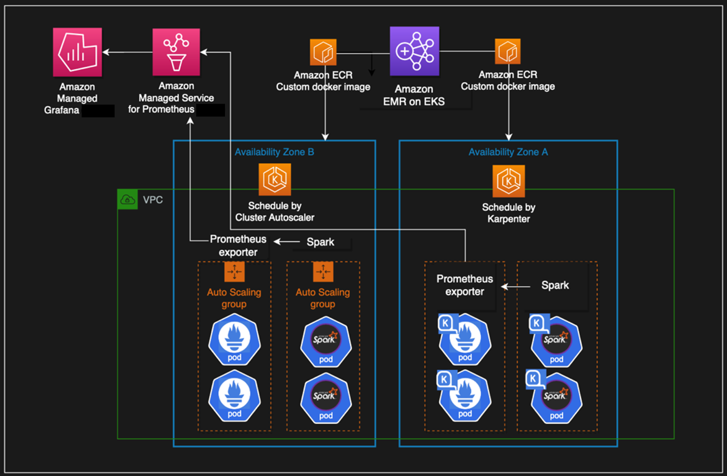
Prerequisites

Before you get started, make sure you have the following prerequisites:

Prepare the data

To illustrate the DataBrew functionality to support data analysis for nested JSON files, we use a publicly available sample customer order details nested JSON dataset.

Complete the following steps to prepare your data:

  1. Sign in to the AWS Management Console.
  2. Browse to the publicly available datasets on the Amazon S3 console.
  3. Select the first dataset (customer_1.json) and choose Download to save the files on your local machine.
  4. Repeat this step to download all three JSON files.

    You can view the sample data from your local machine using any text editor, as shown in the following screenshot.
  5. Create input and output S3 buckets with subfolders nestedjson and outputjson to capture data.
  6. Choose Upload and upload the three JSON files to the nestedjson folder.

Create a DataBrew project

To create your Amazon S3 connection, complete the following steps:

  1. On the DataBrew console, choose Projects in the navigation pane.
  2. Choose Create project.
  3. For Project name, enter Glue-DataBew-NestedJSON-Blog.
  4. Select New dataset.
  5. For Dataset name, enter Glue-DataBew-NestedJSON-Dataset.
  6. For Enter your source from S3, enter the path to the nestedjson folder.
  7. Choose Select the entire folder to select all the files.
  8. Under Additional configurations, select JSON as the file type, then select JSON document.
  9. In the Permissions section, choose Choose existing IAM role if you have one available, or choose Create new IAM role.
  10. Choose Create project.
  11. Skip the preview steps and wait for the project to be ready.
    As shown in the following screenshot, the three JSON files were uploaded to the S3 bucket, so three rows of customer order details are loaded.
    The orders column contains nested files. We can use DataBrew to unnest or nest transform to flatten the columns and rows.
  12. Choose the menu icon (three dots) and choose Nest-unnest.
  13. Depending on the nesting, either choose Unnest to columns or Unnest to rows. In this blog post, we choose Unnest to columns to flatten example JSON file.

    Repeat this step until you get a flattened json for all the nested json data and this will create the AWS Glue Databrew recipe as shown below.
  14. Choose Apply.

    DataBrew automatically creates the required recipe steps with updated column values.
  15. Choose Create job.
  16. For Job name, enter Glue-DataBew-NestedJSON-job.
  17. For S3 location, enter the path to the outputjson folder.
  18. In the Permissions section, for Role name, choose the role you created earlier.
  19. Choose Create and run job.

On the Jobs page, you can choose the job to view its run history, details, and data lineage.

Profile the metadata with DataBrew

After you have a flattened file in the S3 output bucket, you can use DataBrew to carry out the data analysis and profiling for the flattened file. Complete the following steps:

  1. On the Datasets page, choose Connect new datasets.
  2. Provide your dataset details and choose Create dataset.
  3. Choose the newly added data source, then choose the Data profile overview tab.
  4. Enter the name of the job and the S3 path to save the output.
  5. Choose Create and run job.

The job takes around two minutes to complete and display all the updated information. You can explore the data further on the Data profile overview and Column statistics tabs.

Visualize the data in QuickSight

After you have the output file generated by DataBrew in the S3 output bucket, you can use QuickSight to query the JSON data. QuickSight is a scalable, serverless, embeddable, ML-powered business intelligence (BI) service built for the cloud. QuickSight lets you easily create and publish interactive BI dashboards that include ML-powered insights. QuickSight dashboards can be accessed from any device, and seamlessly embedded into your applications, portals, and websites.

Launch QuickSight

On the console, enter quicksight into the search bar and choose QuickSight.

You’re presented with the QuickSight welcome page. If you haven’t signed up for QuickSight, you may have to complete the signup wizard. For more information, refer to Signing up for an Amazon QuickSight subscription.

After you have signed up, QuickSight presents a “Welcome wizard.” You can view the short tutorial, or you can close it.

Grant Amazon S3 access

To grant Amazon S3 access, complete the following steps:

  1. On the QuickSight console, choose your user name, choose Manage QuickSight, then choose Security & permissions.
  2. Choose Add or remove.
  3. Locate Amazon S3 in the list. Choose one of the following:
    1. If the check box is clear, select Amazon S3.
    2. If the check box is already selected, choose Details, then choose Select S3 buckets.
  4. Choose the buckets that you want to access from QuickSight, then choose Select.
  5. Choose Update.
  6. If you changed your Region during the first step of this process, change it back to the Region that you want to use.

Create a dataset

Now that you have QuickSight up and running, you can create your dataset. Complete the following steps:

  1. On the QuickSight console, choose Datasets in the navigation pane.
  2. Choose New dataset.

    QuickSight supports several data sources. For a complete list, refer to Supported data sources.
  3. For your data source, choose S3.

    The S3 import requires a data source name and a manifest file.
  4. On your machine, use a text editor to create a manifest file called BlogGlueDataBrew.manifest using the following structure (provide the name of the your output bucket):
    {
        "fileLocations": [
            {
                "URIPrefixes": [
                "https://s3.amazonaws.com/ s3://<output bucket>/outputjson/"
                ]
            }
        ],
        "globalUploadSettings": {
            "format": "CSV",
            "delimiter": ","
        }
    }

    The manifest file points to the folder that you created earlier as part of your DataBrew project. For more information, refer to Supported formats for Amazon S3 manifest files.

  5. Select Upload and navigate to the manifest file to upload it.
  6. Choose Connect to upload data into SPICE, which is an in-memory database built into QuickSight to achieve fast performance.
  7. Choose Visualize.

You can now create visuals by adding different fields.

To learn more about authoring dashboards in QuickSight, check out the QuickSight Author Workshop.

Clean up

Complete the following steps to avoid incurring future charges:

  1. On the DataBrew console, choose Projects in the navigation pane.
  2. Select the project you created and on the Actions menu, choose Delete.
  3. Choose Jobs in the navigation pane.
  4. Select the job you created and on the Actions menu, choose Delete.
  5. Choose Recipes in the navigation pane.
  6. Select the recipe you created and on the Actions menu, choose Delete.
  7. On the QuickSight dashboard, choose your user name on the application bar, then choose Manage QuickSight.
  8. Choose Account settings, then choose Delete account.
  9. Choose Delete account.
  10. Enter confirm and choose Delete account.

Conclusion

This post walked you through the steps to configure DataBrew to work with nested JSON objects and use QuickSight for data visualization. We used Glue DataBrew to unnest our JSON file and profile the data, and then used QuickSight to create dashboards and visualizations for further analysis.

You can use this solution for your own use cases when you need to unnest complex semi-structured JSON files without writing code. If you have comments or feedback, please leave them in the comments section.


About the authors

Sriharsh Adari is a Senior Solutions Architect at Amazon Web Services (AWS), where he helps customers work backwards from business outcomes to develop innovative solutions on AWS. Over the years, he has helped multiple customers on data platform transformations across industry verticals. His core area of expertise include Technology Strategy, Data Analytics, and Data Science. In his spare time, he enjoys playing sports, binge-watching TV shows, and playing Tabla.

Rahul Sonawane is a Principal Analytics Solutions Architect at AWS with AI/ML and Analytics as his area of specialty.

Amogh Gaikwad is a Solutions Developer at Amazon Web Services. He helps global customers build and deploy AI/ML solutions. His work is mainly focused on computer vision, and NLP uses-cases and helping customers optimize their AI/ML workloads for sustainability. Amogh has received his master’s in Computer Science specializing in Machine Learning.

Ingest VPC flow logs into Splunk using Amazon Kinesis Data Firehose

Post Syndicated from Ranjit Kalidasan original https://aws.amazon.com/blogs/big-data/ingest-vpc-flow-logs-into-splunk-using-amazon-kinesis-data-firehose/

In September 2017, during the annual Splunk.conf, Splunk and AWS jointly announced Amazon Kinesis Data Firehose integration to support Splunk Enterprise and Splunk Cloud as a delivery destination. This native integration between Splunk Enterprise, Splunk Cloud, and Kinesis Data Firehose is designed to make AWS data ingestion setup seamless, while offering a secure and fault-tolerant delivery mechanism. We want to enable you to monitor and analyze machine data from any source and use it to deliver operational intelligence and optimize IT, security, and business performance.

With Kinesis Data Firehose, you can use a fully managed, reliable, and scalable data streaming solution to Splunk. In September 2022, AWS announced a new Amazon Virtual Private Cloud (Amazon VPC) feature that enables you to create VPC flow logs to send the flow log data directly into Kinesis Data Firehose as a destination. Previously, you could send VPC flow logs to either Amazon CloudWatch Logs or Amazon Simple Storage Service (Amazon S3) before it was ingested by other AWS or Partner tools. In this post, we show you how to use this feature to set up VPC flow logs for ingesting into Splunk using Kinesis Data Firehose.

Overview of solution

We deploy the following architecture to ingest data into Splunk.

We create a VPC flow log in an existing VPC to send the flow log data to a Kinesis Data Firehose delivery stream. This delivery stream has an AWS Lambda function enabled for data transformation and has destination settings to point to the Splunk endpoint along with an HTTP Event Collector (HEC) token.

Prerequisites

Before you begin, ensure that you have the following prerequisites:

  • AWS account – If you don’t have an AWS account, you can create one. For more information, see Setting Up for Amazon Kinesis Data Firehose.
  • Splunk AWS Add-on – Ensure you install the Splunk AWS Add-on app from Splunkbase in your Splunk deployment. This app provides the required source types and event types mapping to AWS machine data.
  • HEC token – In your Splunk deployment, set up an HEC token with the source type aws:cloudwatchlogs:vpcflow.

Create the transformation Lambda function

Integrating VPC flow logs with Kinesis Data Firehose requires a Lambda function to transform the flow log records. The data that VPC flow logs sends to the delivery stream is encoded as JSON records. However, Splunk expects this as raw flow log data. Therefore, when you create the delivery stream, you enable data transformation and configure a Lambda function to transform the flow log data to raw format. Kinesis Data Firehose then sends the data in raw format to Splunk.
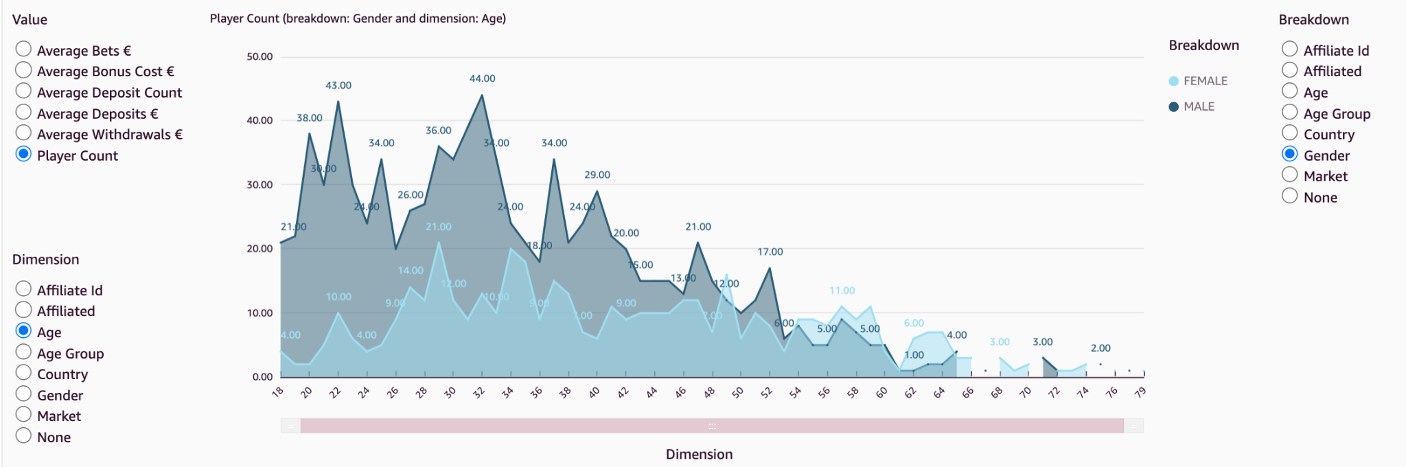
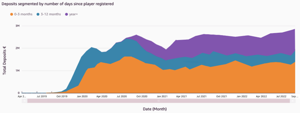
You can deploy this transformation Lambda function as a serverless application from the Lambda serverless app repository on the Lambda console. The name of this application is splunk-firehose-flowlogs-processor.

After it’s deployed, you can see a Lambda function and an AWS Identity and Access Management (IAM) role getting deployed on the console. Note the physical ID of the Lambda function; you use this when you create the Firehose delivery stream in the next step.

Create a Kinesis Data Firehose delivery stream

In this step, you create a Kinesis Data Firehose delivery stream to receive the VPC flow log data and deliver that data to Splunk.

  1. On the Kinesis Data Firehose console, create a new delivery stream.
  2. For Source, choose Direct PUT.
  3. For Destination, choose Splunk.
  4. For Delivery stream name, enter a name (for example, VPCtoSplunkStream).
  5. In the Transform records section, for Data transformation, select Enabled.
  6. For AWS Lambda function, choose Browse.
  7. Select the function you created earlier by looking for the physical ID.
  8. Choose Choose.
  9. In the Destination settings section, for Splunk cluster endpoint, enter your endpoint.If you’re using a Splunk Cloud endpoint, refer to Configure Amazon Kinesis Firehose to send data to the Splunk platform for different Splunk cluster endpoint values.
  10. For Splunk endpoint type, select Raw endpoint.
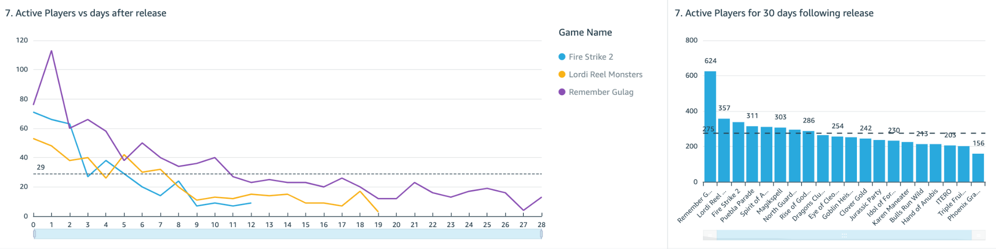
  11. For Authentication token, enter the value of your Splunk HEC that you created as a prerequisite.
  12. In the Backup settings section, for Source record backup in Amazon S3, select Failed events only so you only save the data that fails to be ingested into Splunk.
  13. For S3 backup bucket, enter the path to an S3 bucket.
  14. Complete creating your delivery stream.

The creation process may take a few minutes to complete.

Create a VPC flow log

In this final step, you create a VPC flow log with Kinesis Data Firehose as destination type.

  1. On the Amazon VPC console, choose Your VPCs.
  2. Select the VPC for which to create the flow log.
  3. On the Actions menu, choose Create flow log.
  4. Provide the required settings for Filter:
    1. If you want to filter the flow logs, select Accept traffic or Reject traffic.
    2. Select All if you need all the information sent to Splunk.
  5. For Maximum aggregation interval, select a suitable interval for your use case.Select the minimum setting of 1 minute interval if you need the flow log data to be available for near-real-time analysis in Splunk.
  6. For Destination, select Send to Kinesis Firehose in the same account if the delivery stream is set up on the same account where you create the VPC flow logs.If you want to send the data to a different account, refer to Publish flow logs to Kinesis Data Firehose.
  7. For Log record format, if you leave it at AWS default format, the flow logs are sent as version 2 format. Alternatively, you can specify which fields you need to be captured and sent to Splunk.For more information on log format and available fields, refer to Flow log records.
  8. Review all the parameters and create the flow log.Within a few minutes, you should be able to see the data in Splunk.
  9. Open your Splunk console and navigate to the Search tab of the Search & Reporting app.
  10. Run the following SPL query to look at sample VPC flow log records:
    index=<index name> sourcetype="aws:cloudwatchlogs:vpcflow"

Clean up

To avoid incurring future charges, delete the resources you created in the following order:

  1. Delete the VPC flow log.
  2. Delete the Kinesis Data Firehose delivery stream.
  3. Delete the serverless application to delete the transformation Lambda function.
  4. If you created a new VPC and new resources in the VPC, then delete the resources and VPC.

Conclusion

You can use VPC flow log data in multiple Splunk solutions, like the Splunk App for AWS Security Dashboards for traffic analysis or Splunk Security Essentials, which uses the data to provide deeper insights into the security posture of your AWS environment. Using Kinesis Data Firehose to send VPC flow log data into Splunk provides many benefits. This managed service can automatically scale to meet the data demand and provide near-real-time data analysis. Try out this new quick and hassle-free way of sending your VPC flow logs to Splunk Enterprise or Splunk Cloud Platform using Kinesis Data Firehose.

You can deploy this solution today on your AWS account by following the Kinesis Data Firehose Immersion Day Lab for Splunk


About the authors

Ranjit Kalidasan is a Senior Solutions Architect with Amazon Web Services based in Boston, Massachusetts. He is Partner Solutions Architect helping security ISV partners to co-build and co-market solutions with AWS. He brings over 20 years of experience in Information technology helping global customers implement complex solutions for Security & Analytics. You can connect with Ranjit in Linkedin.