Tag Archives: Analytics

Scale AWS SDK for pandas workloads with AWS Glue for Ray

2022-11-28 Abdel Jaidi

Post Syndicated from Abdel Jaidi original https://aws.amazon.com/blogs/big-data/scale-aws-sdk-for-pandas-workloads-with-aws-glue-for-ray/

AWS SDK for pandas is an open-source library that extends the popular Python pandas library, enabling you to connect to AWS data and analytics services using pandas data frames. We’ve seen customers use the library in combination with pandas for both data engineering and AI workloads. Although pandas data frames are simple to use, they have a limitation on the size of data that can be processed. Because pandas is single-threaded, jobs are bounded by the available resources. If the data you need to process is small, this won’t be a problem, and pandas makes analysis and manipulation simple, as well as interactions with many other tools that support machine learning (ML) and visualization. However, as your data size scales, you may run into problems. This can be especially frustrating if you’ve created a promising prototype that can’t be moved to production. In our work with customers, we’ve seen many projects, both in data science and data engineering, that are stuck while they wait for someone to rewrite using a big data framework such as Apache Spark.

We are excited to announce that AWS SDK for pandas now supports Ray and Modin, enabling you to scale your pandas workflows from a single machine to a multi-node environment, with no code changes. The simplest way to do this is to use AWS Glue with Ray, the new serverless option to run distributed Python code announced at AWS re:Invent 2022. AWS SDK for pandas also supports self-managed Ray on Amazon Elastic Compute Cloud (Amazon EC2).

In this post, we show you how you can use pandas to connect to AWS data and analytics services and manipulate data at scale by running on an AWS Glue with Ray job.

Overview of solution

Ray is a unified framework that enables you to scale AI and Python applications. The goal of the project is to take any Python code that’s written on a laptop and scale the workload on a cluster. This innovative framework opens the door to big data processing to a new audience. Previously, the only way to process large datasets on a cluster was to use tools such as Apache Hadoop, Apache Spark, or Apache Flink. These frameworks require additional skills because they provide their own programming model and often require languages such as Scala or Java to fully take advantage of the advanced capabilities. With Ray, you can just use Python to parallelize your code with few modifications.

Although Ray opens the door to big data processing, it’s not enough on its own to distribute pandas-specific methods. That task falls to Modin, a drop-in replacement of pandas, optimized to run in a distributed environment, such as Ray. Modin has the same API as pandas, so you can keep your code the same, but it parallelizes workloads to improve performance.

With today’s announcement, AWS SDK for pandas customers can use both Ray and Modin for their workloads. You have the option of loading data into Modin data frames, instead of regular pandas data frames. By configuring the library to use Ray and Modin, your existing data processing scripts can distribute operations end-to-end, with no code changes. AWS SDK for pandas takes care of parallelizing the read and write operations for your files across the compute cluster.

To use this feature, you can install the release candidate version of awswrangler with the ray and modin extras:

pip install "awswrangler[modin,ray]==3.0.0rc2"

Once installed, you can use the library in your code by importing it with the following statement:

import awswrangler as wr

When you run this code, the SDK for pandas looks for an environmental variable called WR_ADDRESS. If it finds it, it uses this value to send the commands to a remote cluster. If it doesn’t find it, it starts a local Ray runtime on your machine.

The following diagram shows what is happening when you run code that uses AWS SDK for pandas to read data from Amazon Simple Storage Service (Amazon S3) into a Modin data frame, perform a filtering operation, and write the data back to Amazon S3, using a multi-node cluster.

In the first phase, each node reads one or more input files and stores them in memory as blocks. During this phase, the head node builds a mapping reference that tracks the location of each block on the worker nodes. In the second phase, a filter operation is submitted to each node, creating a subset of the data. Finally, each worker node writes its blocks to Amazon S3.

It’s important to note that certain data frame operations (for example groupby or join) may result in the data being shuffled across nodes. Shuffling will also happen if you do partitioned or bucketed writes. This tends to slow down the job because data needs to move between nodes.

If you want to create your own Ray cluster on Amazon EC2, refer to the tutorial Distributing Calls on Ray Remote Cluster. The rest of this post shows you how to run AWS SDK for pandas and Modin on an AWS Glue with Ray job.

Use AWS Glue with Ray

Because AWS Glue with Ray is a fully managed environment, it’s a simple way to run jobs. Both AWS SDK for pandas and Modin are pre-loaded, you don’t need to worry about cluster management or installing the right set of dependencies, and the job auto scales with your workload. To get started, complete the following steps:

Choose Launch Stack to provision an AWS CloudFormation stack in your AWS account:

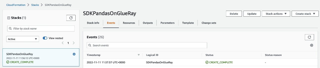
Note that while in preview, AWS Glue with Ray is available in a limited set of AWS Regions.The stack takes about 3 minutes to complete. You can verify that everything was successfully deployed by checking that the CloudFormation stack shows the status CREATE_COMPLETE.
Navigate to AWS Glue Studio to find an AWS Glue job named GlueRayJob with the following script.
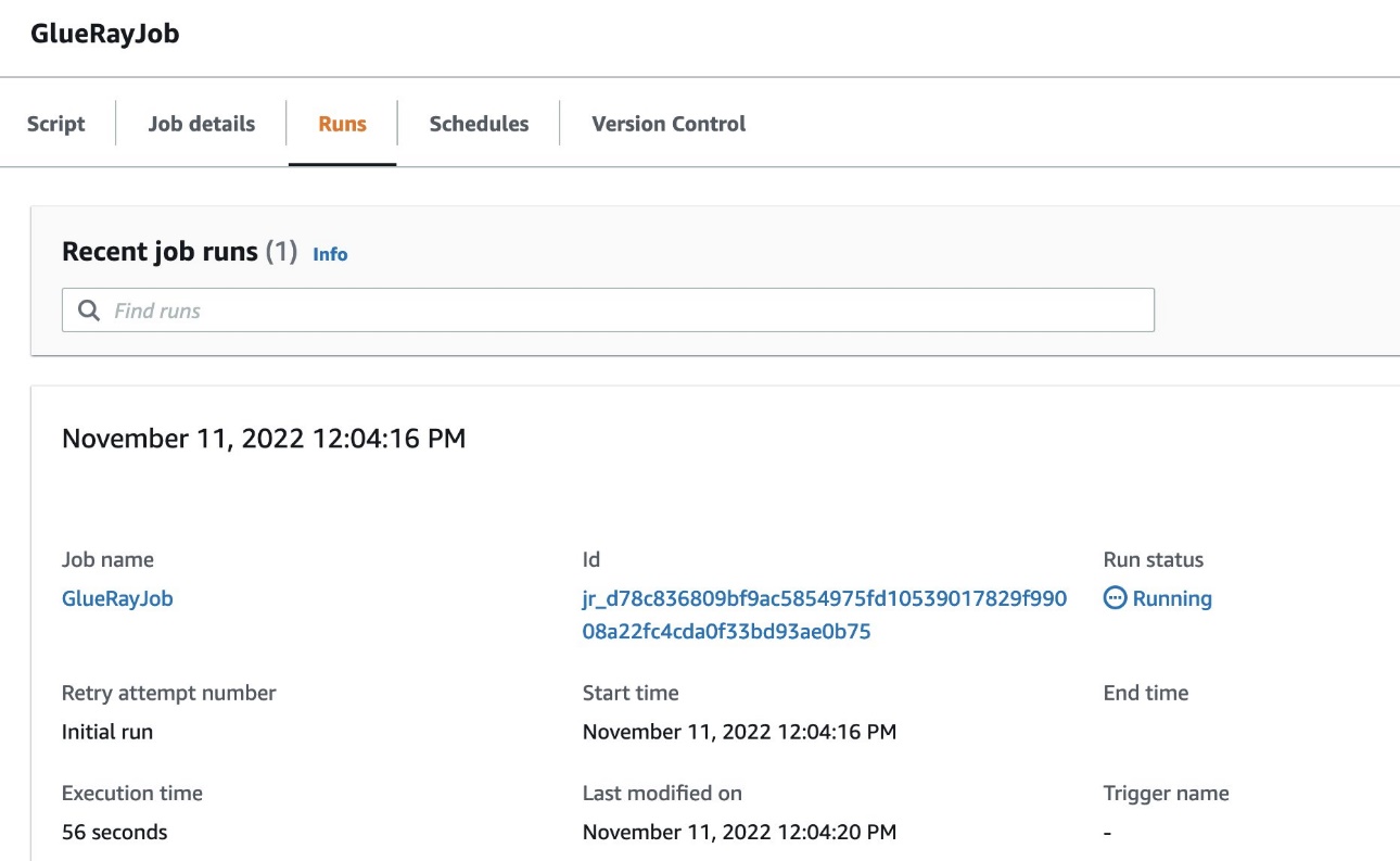
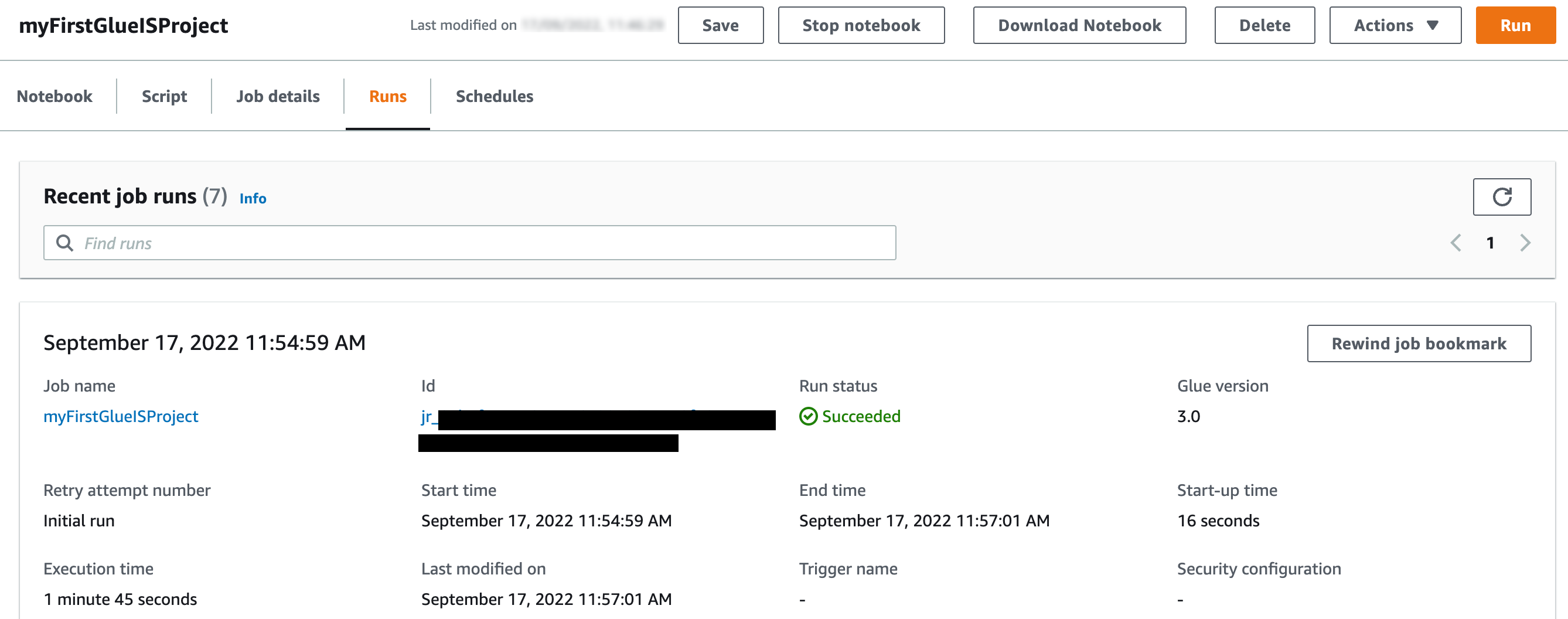
Choose Run to start the job and navigate to the Runs tab to monitor progress.

Here, we break down the script and show you what happens at each stage when we run this code on AWS Glue with Ray. First, we import the library:

import awswrangler as wr

At import, AWS SDK for pandas detects if the runtime supports Ray, and automatically initializes a Ray cluster with the default parameters. In this case, because we’re running on AWS Glue with Ray, AWS SDK for pandas automatically uses the Ray cluster with no extra configuration needed. Advanced users can override this process, however, by starting the Ray runtime before the import command.

Next, we read Amazon product data in Parquet format from Amazon S3 and load it into a distributed Modin data frame:

# Read Parquet data (1.2 Gb Parquet compressed)
df = wr.s3.read_parquet(
    path=f"s3://amazon-reviews-pds/parquet/product_category={category.title()}/",
)

Simple data transformations on the data frame are applied next. Modin data frames implement the same interface as pandas data frames, allowing you to perform familiar pandas operations at scale. First, we drop the customer_id column, then we filter for a subset of the reviews that received five-star ratings:

# Drop the customer_id column
df.drop("customer_id", axis=1, inplace=True)

# Filter reviews with 5-star rating
df5 = df[df["star_rating"] == 5]

The data is written back to Amazon S3 in Parquet format, partitioned by year and marketplace. The dataset=True argument ensures that an associated Hive table is also created in the AWS Glue metadata catalog:

# Write partitioned five-star reviews to S3 in Parquet format
wr.s3.to_parquet(
    df5,
    path=f"s3://{bucket_name}/{category}/",
    partition_cols=["year", "marketplace"],
    dataset=True, 
    database=glue_database,
    table=glue_table, 
)

Finally, a query is run in Amazon Athena, and the S3 objects resulting from this operation are read in parallel into a Modin data frame:

# Read the data back to a Modin df via Athena
df5_athena = wr.athena.read_sql_query(
    f"SELECT * FROM {glue_table}",
    database=glue_database,
    ctas_approach=False, 
    unload_approach=True, 
    workgroup=workgroup_name,
    s3_output=f"s3://{bucket_name}/unload/{category}/",
)

The Amazon CloudWatch logs of the job provide insights into the performance achieved from reading blocks in parallel in a multi-node Ray cluster.

For simplicity, this example showcased Amazon S3 and Athena APIs only, but AWS SDK for pandas supports other services, including Amazon Timestream and Amazon Redshift. For a full list of the APIs that support distribution, refer to Supported APIs.

Clean up AWS resources

To prevent unwanted charges to your AWS account, you can delete the AWS resources that you used for this example:

On the Amazon S3 console, empty data from both buckets with prefix glue-ray-.
On the AWS CloudFormation console, delete the SDKPandasOnGlueRay stack.

The resources created as part of the stack are automatically deleted with it.

Conclusion

In this post, we demonstrated how you can run your workloads at scale using AWS SDK for pandas. When used in combination with AWS Glue with Ray, this gives you access to a fully managed environment to distribute your Python scripts. We hope this solution can help with migrating your existing pandas jobs to achieve higher performance and speedups across multiple data stores on AWS.

For more examples, check out the tutorials in the AWS SDK for pandas documentation.

About the Authors

Abdel Jaidi is a Senior Cloud Engineer for AWS Professional Services. He works on open-source projects focused on AWS Data & Analytics services. In his spare time, he enjoys playing tennis and hiking.

Anton Kukushkin is a Data Engineer for AWS Professional Services based in London, United Kingdom. He works with AWS customers, helping them build and scale their data and analytics.

Leon Luttenberger is a Data Engineer for AWS Professional Services based in Austin, Texas. He works on AWS open-source solutions that help our customers analyze their data at scale.

Lucas Hanson is Senior Cloud Engineer for AWS Professional Services. He focuses on helping customers with infrastructure management and DevOps processes for data management solutions. Outside of work, he enjoys music production and practicing yoga.

Introducing AWS Glue for Ray: Scaling your data integration workloads using Python

2022-11-28 Zach Mitchell

Post Syndicated from Zach Mitchell original https://aws.amazon.com/blogs/big-data/introducing-aws-glue-for-ray-scaling-your-data-integration-workloads-using-python/

AWS Glue is a serverless data integration service that makes it simple to discover, prepare, move, and integrate data from multiple sources for analytics, machine learning (ML), and application development. Today, AWS Glue processes customer jobs using either Apache Spark’s distributed processing engine for large workloads or Python’s single-node processing engine for smaller workloads. Customers like Python for its ease of use and rich collection of built-in data-processing libraries but might find it difficult for customers to scale Python beyond a single compute node. This limitation makes it difficult for customers to process large datasets. Customers want a solution that allows them to continue using familiar Python tools and AWS Glue jobs on data sets of all sizes, even those that can’t fit on a single instance.

We are happy to announce the release of a new AWS Glue job type: Ray. Ray is an open-source unified compute framework that makes it simple to scale AI and Python workloads. Ray started as an open-source project at RISELab in UC Berkeley. If your application is written in Python, you can scale it with Ray in a distributed cluster in a multi-node environment. Ray is Python native and you can combine it with the AWS SDK for pandas to prepare, integrate and transform your data for running your data analytics and ML workloads in combination.

This post provides an introduction to AWS Glue for Ray and shows you how to start using Ray to distribute your Python workloads.

What is AWS Glue for Ray?

Customers like the serverless experience and fast start time offered by AWS Glue. With the introduction of Ray, we have ensured that you get the same experience. We have also ensured that you can use the AWS Glue job and AWS Glue interactive session primitives to access the Ray engine. AWS Glue jobs are fire-and-forget systems where customer submit their Ray code to the AWS Glue jobs API and AWS Glue automatically provisions the required compute resources and runs the job. AWS Glue interactive session APIs allow interactive exploration of the data for the purpose of job development. Regardless of the option used, you are only billed for the duration of the compute used. With AWS Glue for Ray, we are also introducing a new Graviton2 based worker (Z.2x) which offers 8 virtual CPUs and 64 GB of RAM.

AWS Glue for Ray consists of two major components:

Ray Core – The distributed computing framework
Ray Dataset – The distributed data framework based on Apache Arrow

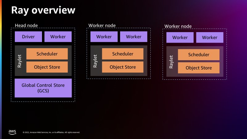
When running a Ray job, AWS Glue provisions the Ray cluster for you and runs these distributed Python jobs on a serverless auto-scaling infrastructure. The cluster in AWS Glue for Ray will consists of exactly one head node and one or more worker nodes.

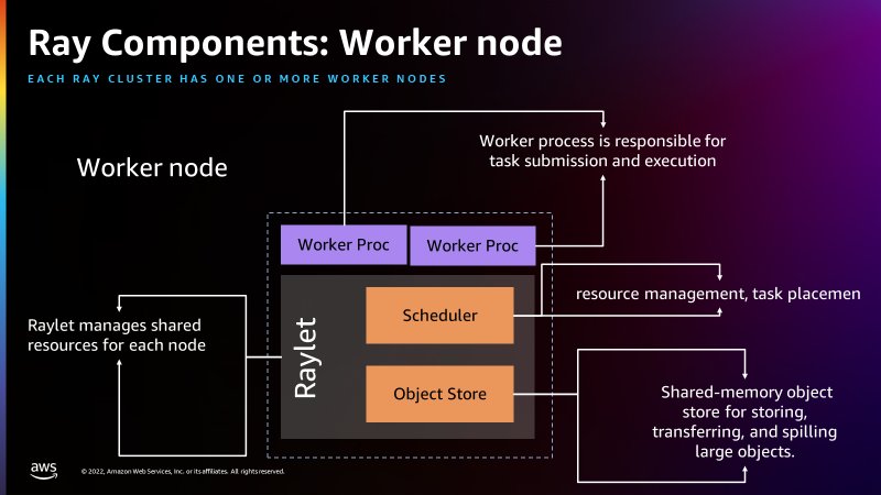
The head node is identical to the other worker nodes with the exception that it runs singleton processes for cluster management and the Ray driver process. The driver is a special worker process in the head node that runs the top-level application in Python that starts the Ray job. The worker node has processes that are responsible for submitting and running tasks.

The following figure provides a simple introduction to the Ray architecture. The architecture illustrates how Ray is able to schedule jobs through processes called Raylets. The Raylet manages the shared resources on each node and is shared between the concurrently running jobs. For more information on how Ray works, see Ray.io.

The following figure shows the components of the worker node and the shared-memory object store:

There is a Global Control Store in the head node that can treat each separate machine as nodes, similar to how Apache Spark treats workers as nodes. The following figure shows the components of the head node and the Global Control Store managing the cluster-level metadata.

AWS Glue for Ray comes included with Ray Core, Ray Dataset, Modin (distributed pandas) and the AWS SDK for pandas (on Modin) for seamless distributed integration into other AWS services. Ray Core is the foundation of Ray and the basic framework for distributing Python functions and classes. Ray Dataset is a distributed data framework based on Apache Arrow and is most closely analogous to a dataframe in Apache Spark. Modin is a library designed to distribute pandas applications across a Ray cluster without any modification and is compatible with data in Ray Datasets. The included AWS SDK for pandas (formerly AWS Data Wrangler) is an abstraction layer on top of Modin to allow for the creation of pandas dataframes from (and writing to) many AWS sources such as Amazon Simple Storage Service (Amazon S3), Amazon Redshift, Amazon DynamoDB, Amazon OpenSearch Service, and others.

You can also install your own ARM compatible Python libraries via pip, either through Ray’s environmental configuration in @ray.remote or via --additional-python-modules.

To learn more about Ray, please visit the GitHub repo.

Why use AWS Glue for Ray?

Many of us start our data journey on AWS with Python, looking to prepare data for ML and data science, and move data at scale with AWS APIs and Boto3. Ray allows you to bring those familiar skills, paradigms, frameworks and libraries to AWS Glue and make them scale to handle massive datasets with minimal code changes. You can use the same data processing tools you currently have (such as Python libraries for data cleansing, computation, and ML) on datasets of all sizes. AWS Glue for Ray enables the distributed run of your Python scripts over multi-node clusters.

AWS Glue for Ray is designed for the following:

Task parallel applications (for example, when you want to apply multiple transforms in parallel)
Speeding up your Python workload as well as using Python native libraries.
Running the same workload across hundreds of data sources.
ML ingestion and parallel batch inference on data

Solution overview

For this post, you will use the Parquet Amazon Customer Reviews Dataset stored in the public S3 bucket. The objective is to perform transformations using the Ray dataset and then write it back to Amazon S3 in the Parquet file format.

Configure Amazon S3

The first step is to create an Amazon S3 bucket to store the transformed Parquet dataset as the end result.

On the Amazon S3 console, choose Buckets in the navigation pane.
Choose Create bucket.
For Bucket name, enter a name for your Amazon S3 bucket.
Choose Create.

Set up a Jupyter notebook with an AWS Glue interactive session

For our development environment, we use a Jupyter notebook to run the code.

You’re required to install the AWS Glue interactive sessions locally or run interactive sessions with an AWS Glue Studio notebook. Using AWS Glue Interactive sessions will help you follow and run the series of demonstration steps.

Refer to Getting started with AWS Glue interactive sessions for instructions to spin up a notebook on an AWS Glue interactive session.

Run your code using Ray in a Jupyter notebook

This section walks you through several notebook paragraphs on how to use AWS Glue for Ray. In this exercise, we look at the customer reviews from the Amazon Customer Review Parquet dataset, perform some Ray transformations, and write the results to Amazon S3 in a Parquet format.

On Jupyter console, under New, choose Glue Python.
Signify you want to use Ray as the engine by using the %glue_ray magic.

Import the Ray library along with additional Python libraries:

%glue_ray

import ray
import pandas
import pyarrow
from ray import data
import time
from ray.data import ActorPoolStrategy

Initialize a Ray Cluster with AWS Glue.
```
ray.init('auto')
```

Next, we read a single partition from the dataset, which is Parquet file format:

start = time.time()
ds = ray.data.read_parquet("s3://amazon-reviews-pds/parquet/product_category=Wireless/")
end = time.time()
print(f"Reading the data to dataframe: {end - start} seconds")

Parquet files store the number of rows per file in the metadata, so we can get the total number of records in ds without performing a full data read:
```
ds.count()
```
Next , we can check the schema of this dataset. We don’t have to read the actual data to get the schema; we can read it from the metadata:
```
ds.schema()
```

We can check the total size in bytes for the full Ray dataset:

#calculate the size in bytes of the full dataset,  Note that for Parquet files, this size-in-bytes will be pulled from the Parquet
#  metadata (not triggering a data read).
ds.size_bytes()

We can see a sample record from the Ray dataset:

#Show sample records from the underlying Parquet dataset  
start = time.time()
ds.show(1)
end = time.time()
print(f"Time taken to show the data from dataframe : {end - start} seconds")

Applying dataset transformations with Ray

There are primarily two types of transformations that can be applied to Ray datasets:

One-to-One transformations – Each input block will contributes to only one output block, such as add_column(), map_batches() and drop_column() , and so on.
All-to-All transformations – Input blocks can contribute to multiple output blocks such as sort() and groupby(), and so on.

In the next series of steps we will apply some of these transformations on our resultant Ray datasets from the previous section.

We can add a new column and check the schema to verify the newly added column, followed by retrieving a sample record. This transformation is only available for the datasets that can be converted to pandas format.

# Add the given new column to the dataset and show the sample record after adding a new column

start = time.time()
ds = ds.add_column( "helpful_votes_ratio", lambda df: df["helpful_votes"] / df["total_votes"])
end = time.time()
print(f"Time taken to Add a new columns : {end - start} seconds")
ds.show(1)

Let’s drop a few columns we don’t need using a drop_columns transformation and then check the schema to verify if those columns are dropped from the Ray dataset:
```
# Dropping few columns from the underlying Dataset 
start = time.time()
ds = ds.drop_columns(["review_body", "vine", "product_parent", "verified_purchase", "review_headline"])
end = time.time()
print(f"Time taken to drop a few columns : {end - start} seconds")
ds.schema()
```
Ray datasets have built-in transformations such as sorting the dataset by the specified key column or key function.

Next, we apply the sort transformation using one of the columns present in the dataset (total_votes):

#Sort the dataset by total votes
start = time.time()
ds =ds.sort("total_votes")
end = time.time()
print(f"Time taken for sort operation  : {end - start} seconds")
ds.show(3)

Next, we will create a Python UDF function that allows you to write customized business logic in transformations. In our UDF we have written a logic to find out the products that are rated low (i.e. total votes less than 100).We create a UDF as a function on pandas DataFrame batches. For the supported input batch formats, see the UDF Input Batch Format. We also demonstrate using map_batches() which applies the given function to the batches of records of this dataset. Map_batches() uses the default compute strategy (tasks), which helps distribute the data processing to multiple Ray workers, which are used to run tasks. For more information on a map_batches() transformation, please see the following documentation.
```
# UDF as a function on pandas DataFrame - To Find products with total_votes < 100 
def low_rated_products(df: pandas.DataFrame) -> pandas.DataFrame:
    return df[(df["total_votes"] < 100)]
    
#Calculate the number of products which are rated low in terms of low votes i.e. less than 100
# This technique is called Batch inference processing with Ray tasks (the default compute strategy).
ds = ds.map_batches(low_rated_products)

#See sample records for the products which are rated low in terms of low votes i.e. less than 100
ds.show(1)
```
```
#Count total number of products which are rated low 
ds.count()
```

If you have complex transformations that require more resources for data processing, we recommend utilizing Ray actors using additional configurations with applicable transformations. We have demonstrated with map_batches() below:

# Batch inference processing with Ray actors. Autoscale the actors between 2 and 4.

class LowRatedProducts:
    def __init__(self):
        self._model = low_rated_products

    def __call__(self, batch: pandas.DataFrame) -> pandas.DataFrame:
        return self._model(batch)

start = time.time()
predicted = ds.map_batches(
    LowRatedProducts, compute=ActorPoolStrategy(2, 4), batch_size=4)
end = time.time()

Next, before writing the final resultant Ray dataset we will apply map_batches() transformations to filter out the customer reviews data where the total votes for a given product is greater than 0 and the reviews belongs to the “US” marketplace only. Using map_batches() for the filter operation is better in terms of performance in comparison to filter() transformation.
```
# Filter our records with total_votes == 0
ds = ds.map_batches(lambda df: df[df["total_votes"] > 0])

# Filter and select records with marketplace equals US only
ds = ds.map_batches(lambda df: df[df["marketplace"] == 'US'])

ds.count()
```
Finally, we write the resultant data to the S3 bucket you created in a Parquet file format. You can use different dataset APIs available, such as write_csv() or write_json() for different file formats. Additionally, you can convert the resultant dataset to another DataFrame type such as Mars, Modin or pandas.
```
ds.write_parquet("s3://<your-own-s3-bucket>/manta/Output/Raydemo/")
```

Clean up

To avoid incurring future charges, delete the Amazon S3 bucket and Jupyter notebook.

On the Amazon S3 console, choose Buckets.
Choose the bucket you created.
Choose Empty and enter your bucket name.
Choose Confirm.
Choose Delete and enter your bucket name.
Choose Delete bucket.
On the AWS Glue console, choose Interactive Sessions
Choose the interactive session you created.
Choose Delete to remove the interactive session.

Conclusion

In this post, we demonstrated how you can use AWS Glue for Ray to run your Python code in a distributed environment. You can now run your data and ML applications in a multi-node environment.

Refer to the Ray documentation for additional information and use cases.

About the authors

Zach Mitchell is a Sr. Big Data Architect. He works within the product team to enhance understanding between product engineers and their customers while guiding customers through their journey to develop data lakes and other data solutions on AWS analytics services.

Ishan Gaur works as Sr. Big Data Cloud Engineer ( ETL ) specialized in AWS Glue. He’s passionate about helping customers build out scalable distributed ETL workloads and implement scalable data processing and analytics pipelines on AWS. When not at work, Ishan likes to cook, travel with his family, or listen to music.

Derek Liu is a Solutions Architect on the Enterprise team based out of Vancouver, BC. He is part of the AWS Analytics field community and enjoys helping customers solve big data challenges through AWS analytic services.

Kinshuk Pahare is a Principal Product Manager on AWS Glue.

New – Amazon Redshift Support in AWS Backup

2022-11-28 Danilo Poccia

Post Syndicated from Danilo Poccia original https://aws.amazon.com/blogs/aws/new-amazon-redshift-support-in-aws-backup/

With Amazon Redshift, you can analyze data in the cloud at any scale. Amazon Redshift offers native data protection capabilities to protect your data using automatic and manual snapshots. This works great by itself, but when you’re using other AWS services, you have to configure more than one tool to manage your data protection policies.

To make this easier, I am happy to share that we added support for Amazon Redshift in AWS Backup. AWS Backup allows you to define a central backup policy to manage data protection of your applications and can now also protect your Amazon Redshift clusters. In this way, you have a consistent experience when managing data protection across all supported services. If you have a multi-account setup, the centralized policies in AWS Backup let you define your data protection policies across all your accounts within your AWS Organizations. To help you meet your regulatory compliance needs, AWS Backup now includes Amazon Redshift in its auditor-ready reports. You also have the option to use AWS Backup Vault Lock to have immutable backups and prevent malicious or inadvertent changes.

Let’s see how this works in practice.

Using AWS Backup with Amazon Redshift
The first step is to turn on the Redshift resource type for AWS Backup. In the AWS Backup console, I choose Settings in the navigation pane and then, in the Service opt-in section, Configure resources. There, I toggle the Redshift resource type on and choose Confirm.

Now, I can create or update a backup plan to include the backup of all, or some, of my Redshift clusters. In the backup plan, I can define how often these backups should be taken and for how long they should be kept. For example, I can have daily backups with one week of retention, weekly backups with one month of retention, and monthly backups with one year of retention.

I can also create on-demand backups. Let’s see this with more details. I choose Protected resources in the navigation pane and then Create on-demand backup.

I select Redshift in the Resource type dropdown. In the Cluster identifier, I select one of my clusters. For this workload, I need two weeks of retention. Then, I choose Create on-demand backup.

My data warehouse is not huge, so after a few minutes, the backup job has completed.

I now see my Redshift cluster in the list of the resources protected by AWS Backup.

In the Protected resources list, I choose the Redshift cluster to see the list of the available recovery points.

When I choose one of the recovery points, I have the option to restore the full data warehouse or just a table into a new Redshift cluster.

I now have the possibility to edit the cluster and database configuration, including security and networking settings. I just update the cluster identifier, otherwise the restore would fail because it must be unique. Then, I choose Restore backup to start the restore job.

After some time, the restore job has completed, and I see the old and the new clusters in the Amazon Redshift console. Using AWS Backup gives me a simple centralized way to manage data protection for Redshift clusters as well as many other resources in my AWS accounts.

Availability and Pricing
Amazon Redshift support in AWS Backup is available today in the AWS Regions where both AWS Backup and Amazon Redshift are offered, with the exception of the Regions based in China. You can use this capability via the AWS Management Console, AWS Command Line Interface (CLI), and AWS SDKs.

There is no additional cost for using AWS Backup compared to the native snapshot capability of Amazon Redshift. Your overall costs depend on the amount of storage and retention you need. For more information, see AWS Backup pricing.

— Danilo

New for Amazon Transcribe – Real-Time Analytics During Live Calls

2022-11-28 Danilo Poccia

Post Syndicated from Danilo Poccia original https://aws.amazon.com/blogs/aws/new-for-amazon-transcribe-real-time-analytics-during-live-calls/

The experience customers have when interacting with a contact center can have a profound impact on them. For this reason, we launched Amazon Transcribe Call Analytics last year to help you analyze customer call recordings and get insights into issues and trends related to customer satisfaction and agent performance.

To assist agents in resolving live calls faster, we are introducing today real-time call analytics in Amazon Transcribe Call Analytics. Real-time call analytics provides APIs for developers to accurately transcribe live calls and at the same time identify customer experience issues and sentiment in real time. Transcribe Call Analytics uses state-of-the-art machine learning capabilities to automatically assess thousands of in-progress calls and detect customer experience issues, such as repeated requests to speak to a manager or cancel a subscription.

With a few clicks, supervisors and analysts can create categories in the AWS console to identify customer experience issues using criteria such as specific terms such as “not happy,” “poor quality,” and “cancel my subscription.” Transcribe Call Analytics analyzes in-progress calls in real time to detect when a category is met. Developers can use those signals, along with sentiment trends from the API, to build a proactive system that alerts supervisors about emerging issues or assists agents with relevant information to solve customer issues.

Transcribe Call Analytics also provides a real-time transcript of the live conversation that supervisors can use to quickly get up to speed on the customer interaction and assess the appropriate action. The in-call transcript also eliminates the need for customers to repeat themselves if the call is transferred to another agent. Agents can focus all their attention on the customer during the call instead of taking notes for entry in a CRM system because Transcribe Call Analytics includes an automated call summarization capability, which identifies the issue, outcome, and action item associated with a call.

Transcribe Call Analytics is a foundational API for AWS Contact Center Intelligence solutions such as post-call analytics and the updated real-time call analytics with agent assist solution using the new real-time capabilities.

Let’s see how this works in practice.

Exploring Real-Time Call Analytics in the Console
To see how this works visually, I use the Amazon Transcribe console. First, I create a category to be notified if some terms are used in the call that would require an escalation. I choose Category Management from the navigation pane and then Create category.

I enter Escalation as the name for the category. I select REAL_TIME in the Category type dropdown. Then, I choose Create from scratch.

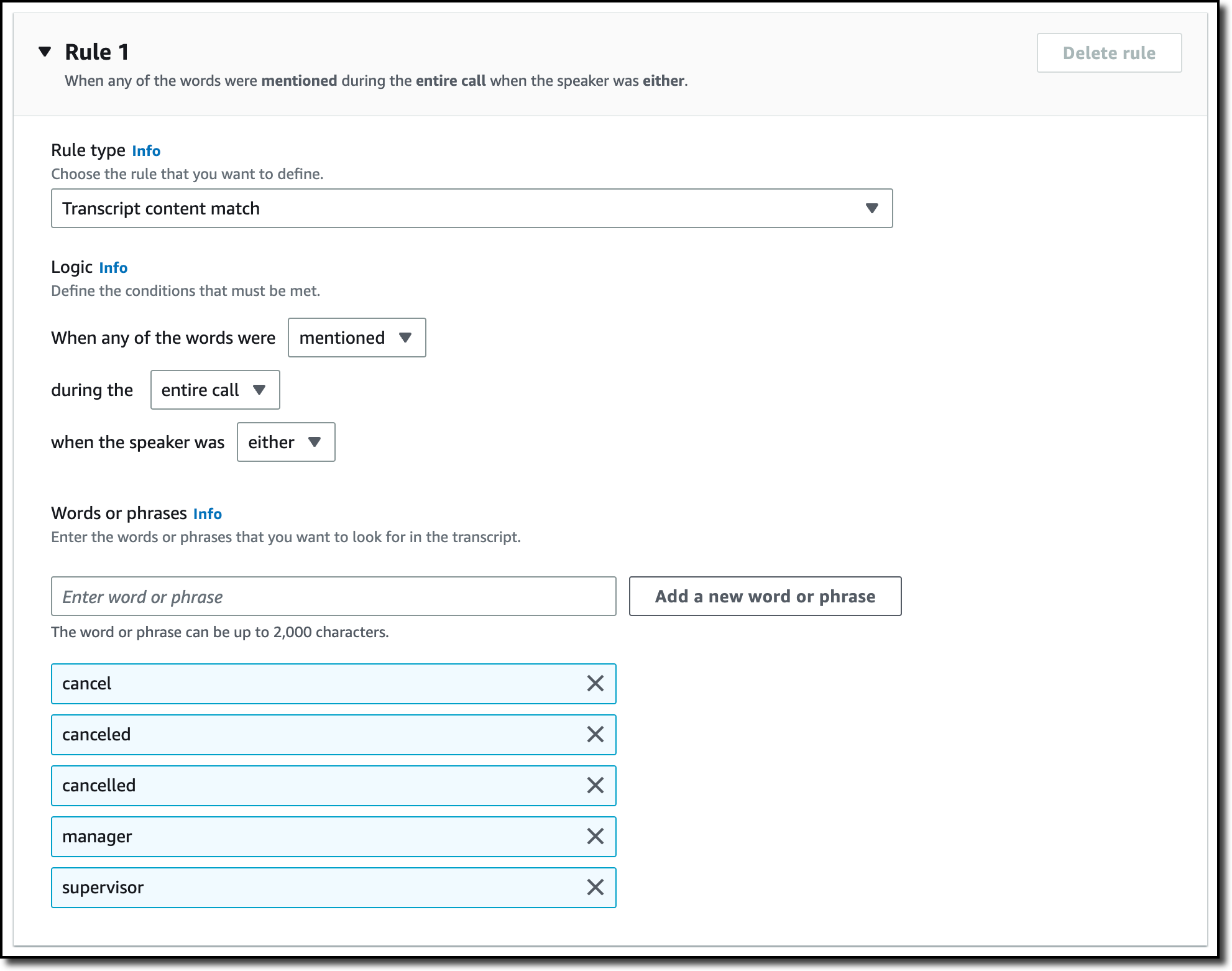
I only need one rule for this category. In the Rule type dropdown, I select Transcript content match. In the next three options, I choose to trigger the rule when any of the words are mentioned during the entire call, and the speaker is either the customer or the agent. Now, I can enter the words or phrases to look for in the transcript. In this case, I enter cancel, canceled, cancelled, manager, and supervisor. In your case, you might be more specific depending on your business. For example, if subscriptions are your business, you can look for the phrase cancel my subscription.

Now that the category has been created, I use one of the sample calls in the console to test it. I choose Real-Time Analytics in the navigation pane. By choosing Configure advanced settings, I can configure the personally identifiable information (PII) identification and redaction settings. For example, I can choose to identify personal data such as email addresses or redact financial data like bank account numbers.

With no additional charge, I can enable Post-call Analytics so that, at the end of the call, I receive the output of the transcription job in an Amazon Simple Storage Service (Amazon S3) bucket. This output is in a similar format to what I’d receive if I were analyzing a call recording with Transcribe Call Analytics. In this way, I can use the post-call analytics output derived from the audio stream in any process I already have in place for output of analytics generated from call recordings, for example, to update dashboards or generate periodic reports.

With Insurance complaints in Step 1: Specify input audio selected, I choose Start streaming. In the Transcription output section of the console, I receive in real-time the transcription of the call. The words of the customer and agent appear as they are pronounced. Each sentence is flagged with its recognized sentiment (positive, neutral, or negative). The Escalation category that I just configured is found in two sentences, first, when the customer mentions that their insurance has been canceled, and then when the agent mentions their manager. Also, part of a sentence is underlined because an issue has been detected.

Using the Download dropdown, I download the full JSON transcript. If I am only interested in the transcription, I can download the text transcript. The JSON transcript contains an array where each item is similar to what I’d get in real time when using the real-time call analytics API.

Using the Live Call Analytics With Agent Assist (LCA) Solution
You can use the open-source real-time call analytics with agent assist solution for your contact center or as an inspiration of what Amazon Transcribe enables for developers. Let’s look at a couple of screenshots to understand how it works.

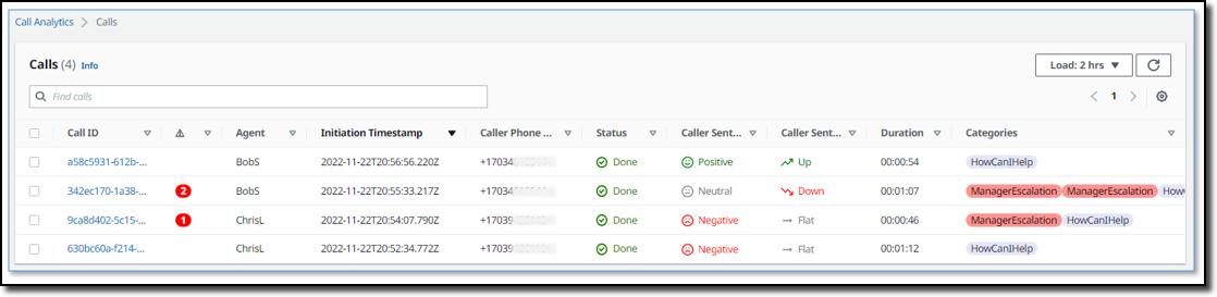
Here there is a list of on-going calls with the overall sentiment, the sentiment trend (is it improving or not?), and the categories found in real-time during the call that can be used for specific activities.

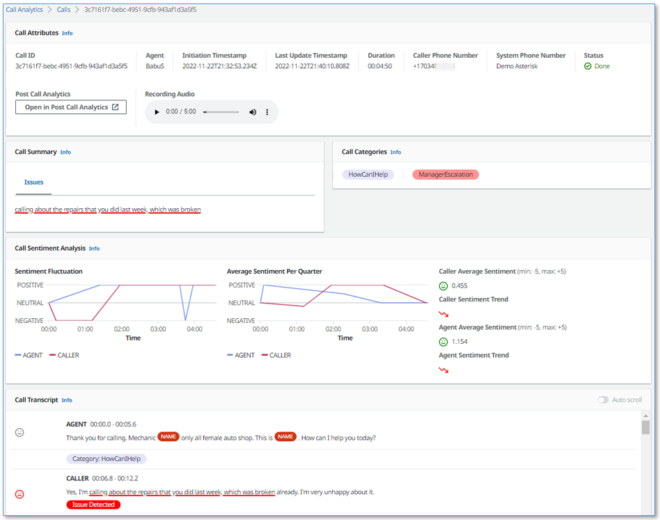
When selecting a call from the list, you have access to more in-depth information, including the call transcript and the issues found during the on-going call. This allows to take action quickly to help resolve the call.

Availability and Pricing
Amazon Transcribe Call Analytics with real-time capabilities is available today in US (N. Virginia, Oregon), Canada (Central), Europe (Frankfurt, London), and Asia Pacific (Seoul, Sydney, Tokyo) and supports US English, British English, Australian English, US Spanish, Canadian French, French, German, Italian, and Brazilian Portuguese.

With Amazon Transcribe Call Analytics, you pay as you go and are billed monthly based on tiered pricing. For more information, see Amazon Transcribe pricing.

As part of the AWS Free Tier, you can get started with Amazon Transcribe Call Analytics for free, including the new real-time call analytics API. You can analyze up to 60 minutes of call audio monthly for free for the first 12 months. For more information, see the AWS Free Tier page.

If you’re at re:Invent, you can learn more about this new capability in session AIM307 – JPMorganChase real-time agent assist for contact center productivity. I will update this post when the recording of the session is publicly available.

Start analyzing contact center conversations in real-time to improve your customers’ experience.

— Danilo

Graph for fraud detection

2022-11-24 Grab Tech

Post Syndicated from Grab Tech original https://engineering.grab.com/graph-for-fraud-detection

Grab has grown rapidly in the past few years. It has expanded its business from ride hailing to food and grocery delivery, financial services, and more. Fraud detection is challenging in Grab, because new fraud patterns always arise whenever we introduce a new business product. We cannot afford to develop a new model whenever a new fraud pattern appears as it is time consuming and introduces a cold start problem, that is no protection at the early stage. We need a general fraud detection framework to better protect Grab from various unknown fraud risks.

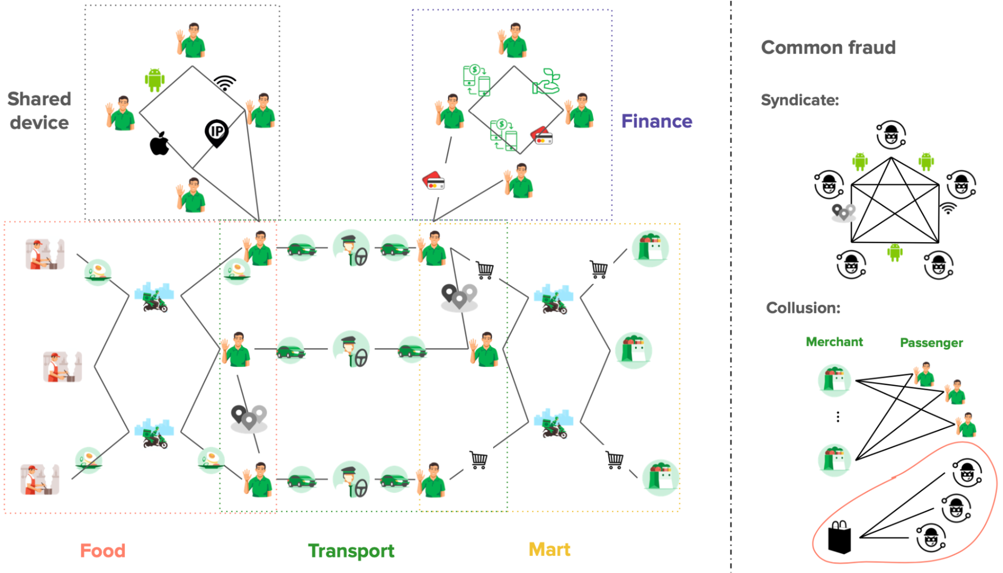
Our key observation is that although Grab has many different business verticals, the entities within those businesses are connected to each other (Figure 1. Left), for example, two passengers may be connected by a Wi-Fi router or phone device, a merchant may be connected to a passenger by a food order, and so on. A graph provides an elegant way to capture the spatial correlation among different entities in the Grab ecosystem. A common fraud shows clear patterns on a graph, for example, a fraud syndicate tends to share physical devices, and collusion happens between a merchant and an isolated set of passengers (Figure 1. Right).

Figure 1. Left: The graph captures different correlations in the Grab ecosystem.
Right: The graph shows that common fraud has clear patterns.

We believe graphs can help us discover subtle traces and complicated fraud patterns more effectively. Graph-based solutions will be a sustainable foundation for us to fight against known and unknown fraud risks.

Why graph?

The most common fraud detection methods include the rule engine and the decision tree-based models, for example, boosted tree, random forest, and so on. Rules are a set of simple logical expressions designed by human experts to target a particular fraud problem. They are good for simple fraud detection, but they usually do not work well in complicated fraud or unknown fraud cases.

Fraud detection methods	Utilises correlations (Higher is better)	Detects unknown fraud (Higher is better)	Requires feature engineering (Lower is better)	Depends on labels (Lower is better)
Rule engine	Low	N/A	N/A	Low
Decision tree	Low	Low	High	High
Graph model	High	High	Low	Low

Table 1. Graph vs. common fraud detection methods.

Decision tree-based models have been dominating fraud detection and Kaggle competitions for structured or tabular data in the past few years. With that said, the performance of a tree-based model is highly dependent on the quality of labels and feature engineering, which is often hard to obtain in real life. In addition, it usually does not work well in unknown fraud which has not been seen in the labels.

On the other hand, a graph-based model requires little amount of feature engineering and it is applicable to unknown fraud detection with less dependence on labels, because it utilises the structural correlations on the graph.

In particular, fraudsters tend to show strong correlations on a graph, because they have to share physical properties such as personal identities, phone devices, Wi-Fi routers, delivery addresses, and so on, to reduce cost and maximise revenue as shown in Figure 2 (left). An example of such strong correlations is shown in Figure 2 (right), where the entities on the graph are densely connected, and the known fraudsters are highlighted in red. Those strong correlations on the graph are the key reasons that make the graph based approach a sustainable foundation for various fraud detection tasks.

Figure 2. Fraudsters tend to share physical properties to reduce cost (left), and they are densely connected as shown on a graph (right).

Semi-supervised graph learning

Unlike traditional decision tree-based models, the graph-based machine learning model can utilise the graph’s correlations and achieve great performance even with few labels. The semi-supervised Graph Convolutional Network model has been extremely popular in recent years ¹. It has proven its success in many fraud detection tasks across industries, for example, e-commerce fraud, financial fraud, internet traffic fraud, etc.
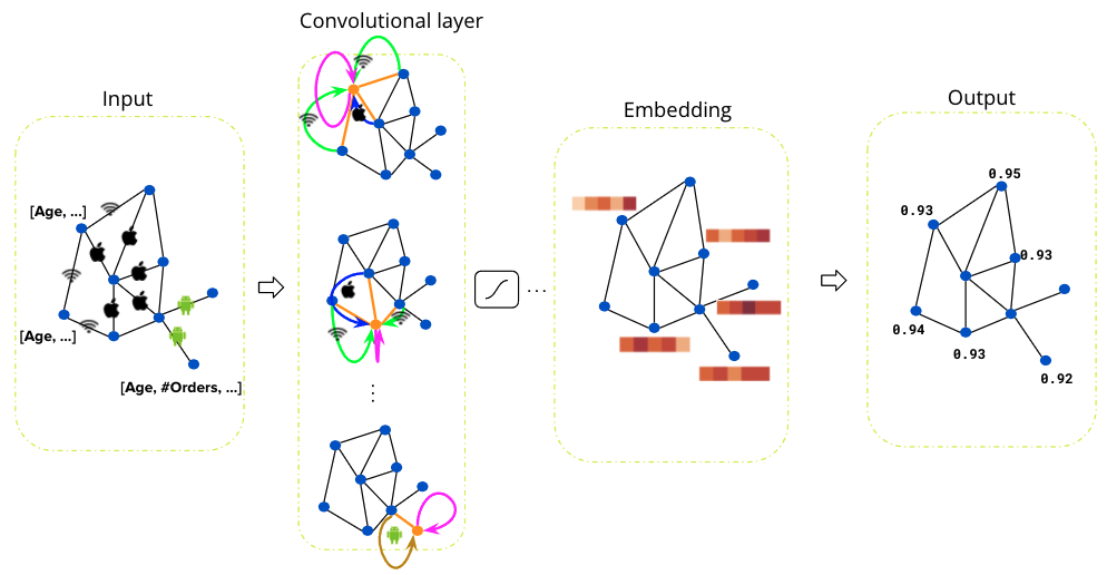
We apply the Relational Graph Convolutional Network (RGCN) ² for fraud detection in Grab’s ecosystem. Figure 3 shows the overall architecture of RGCN. It takes a graph as input, and the graph passes through several graph convolutional layers to get node embeddings. The final layer outputs a fraud probability for each node. At each graph convolutional layer, the information is propagated along the neighbourhood nodes within the graph, that is nodes that are close on the graph are similar to each other.

Fig 3. A semi-supervised Relational Graph Convolutional Network model.

We train the RGCN model on a graph with millions of nodes and edges, where only a few percentages of the nodes on the graph have labels. The semi-supervised graph model has little dependency on the labels, which makes it a robust model for tackling various types of unknown fraud.

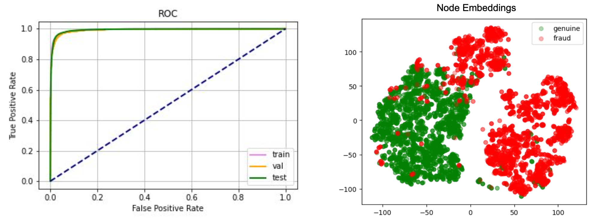
Figure 4 shows the overall performance of the RGCN model. On the left is the Receiver Operating Characteristic (ROC) curve on the label dataset, in particular, the Area Under the Receiver Operating Characteristic (AUROC) value is close to 1, which means the RGCN model can fit the label data quite well. The right column shows the low dimensional projections of the node embeddings on the label dataset. It is clear that the embeddings of the genuine passenger are well separated from the embeddings of the fraud passenger. The model can distinguish between a fraud and a genuine passenger quite well.

Fig 4. Left: ROC curve of the RGCN model on the label dataset.
Right: Low dimensional projections of the graph node embeddings.

Finally, we would like to share a few tips that will make the RGCN model work well in practice.

Use less than three convolutional layers: The node feature will be over-smoothed if there are many convolutional layers, that is all the nodes on the graph look similar.
Node features are important: Domain knowledge of the node can be formulated as node features for the graph model, and rich node features are likely to boost the model performance.

Graph explainability

Unlike other deep network models, graph neural network models usually come with great explainability, that is why a user is classified as fraudulent. For example, fraudulent accounts are likely to share hardware devices and form dense clusters on the graph, and those fraud clusters can be easily spotted on a graph visualiser ³.

Figure 5 shows an example where graph visualisation helps to explain the model prediction scores. The genuine passenger with a low RGCN score does not share devices with other passengers, while the fraudulent passenger with a high RGCN score shares devices with many other passengers, that is, dense clusters.

Figure 5. Upper left: A genuine passenger with a low RGCN score has no device sharing with other passengers. Bottom right: A fraudulent user with a high RGCN score shares devices with many other passengers.

Closing thoughts

Graphs provide a sustainable foundation for combating many different types of fraud risks. Fraudsters are evolving very fast these days, and the best traditional rules or models can do is to chase after those fraudsters given that a fraud pattern has already been discovered. This is suboptimal as the damage has already been done on the platform. With the help of graph models, we can potentially detect those fraudsters before any fraudulent activity has been conducted, thus reducing the fraud cost.

The graph structural information can significantly boost the model performance without much dependence on labels, which is often hard to get and might have a large bias in fraud detection tasks. We have shown that with only a small percentage of labelled nodes on the graph, our model can already achieve great performance.

With that said, there are also many challenges to making a graph model work well in practice. We are working towards solving the following challenges we are facing.

Feature initialisation: Sometimes, it is hard to initialise the node feature, for example, a device node does not carry many semantic meanings. We have explored self-supervised pre-training ⁴ to help the feature initialisation, and the preliminary results are promising.
Real-time model prediction: Realtime graph model prediction is challenging because real-time graph updating is a heavy operation in most cases. One possible solution is to do batch real-time prediction to reduce the overhead.
Noisy connections: Some connections on the graph are inherently noisy on the graph, for example, two users sharing the same IP address does not necessarily mean they are physically connected. The IP might come from a mobile network. One possible solution is to use the attention mechanism in the graph convolutional kernel and control the message passing based on the type of connection and node profiles.

Join us

Grab is the leading superapp platform in Southeast Asia, providing everyday services that matter to consumers. More than just a ride-hailing and food delivery app, Grab offers a wide range of on-demand services in the region, including mobility, food, package and grocery delivery services, mobile payments, and financial services across 428 cities in eight countries.

Powered by technology and driven by heart, our mission is to drive Southeast Asia forward by creating economic empowerment for everyone. If this mission speaks to you, join our team today!

References

T. Kipf and M. Welling, “Semi-supervised classification with graph convolutional networks,” in ICLR, 2017 ↩
Schlichtkrull, Michael, et al. “Modeling relational data with graph convolutional networks.” European semantic web conference. Springer, Cham, 2018. ↩
Fujiao Liu, Shuqi Wang, et al.. “Graph Networks – 10X investigation with Graph Visualisations”. Grab Tech Blog. ↩
Wang, Chen, et al.. “Deep Fraud Detection on Non-attributed Graph.” IEEE Big Data conference, PSBD, 2021. ↩

Implement row-level access control in a multi-tenant environment with Amazon Redshift

2022-11-23 Siva Bangaru

Post Syndicated from Siva Bangaru original https://aws.amazon.com/blogs/big-data/implement-row-level-access-control-in-a-multi-tenant-environment-with-amazon-redshift/

This is a guest post co-written with Siva Bangaru and Leon Liu from ADP.

ADP helps organizations of all types and sizes by providing human capital management (HCM) solutions that unite HR, payroll, talent, time, tax, and benefits administration. ADP is a leader in business outsourcing services, analytics, and compliance expertise. ADP’s unmatched experience, deep insights, and cutting-edge technology have transformed human resources from a back-office administrative function to a strategic business advantage.

People Analytics powered by ADP DataCloud is an application that provides analytics and enhanced insights to ADP’s clients. It delivers a guided analytics experience that make it easy for you to create, use, and distribute tailored analytics for your organization. ADP People Analytics’s streamlined, configurable dashboards can help you identify potential issues in key areas, like overtime, turnover, compensation, and much more.

ADP provides this analytics experience to thousands of clients today. Securing customers’ data is a top priority for ADP. The company requires the highest security standards when implementing a multi-tenant analytics platform on Amazon Redshift.

ADP DataCloud integrates with Amazon Redshift row-level security (RLS) to implement granular data entitlements and enforce the access restrictions on their tables in Amazon Redshift.

In this post, we discuss how the ADP DataCloud team implemented Amazon Redshift RLS on the foundation of role-based access control (RBAC) to simplify managing privileges required in a multi-tenant environment, and also enabled and enforced access to granular data entitlements in business terms.

The ADP DataCloud team had the following key requirements and challenges:

Support a multi-tenant application to enforce a logical separation of each tenant’s data rows
Support dynamic provisioning of new tenants
Minimal impact on performance

Row-level security in Amazon Redshift

Amazon Redshift is a fully managed, petabyte-scale data warehouse service in the cloud. One of the challenges with security is that enterprises want to provide fine-grained access control at the row level for sensitive data. This can be done by creating views or using different databases and schemas for different users. However, this approach isn’t scalable and becomes complex to maintain over time, especially when supporting multi-tenant environments.

In early 2022, Amazon Redshift released row-level security, which is built on the foundation of role-based access control. RLS allows you to control which users or roles can access specific records of data within tables, based on security policies that are defined at the database object level. This new RLS capability in Amazon Redshift enables you to dynamically filter existing rows of data in a table along with session context variable setting capabilities to dynamically assign the appropriate tenant configuration. This is in addition to column-level access control, where you can grant users permissions to a subset of columns. Now you can combine column-level access control with RLS policies to further restrict access to particular rows of visible columns. Refer to Achieve fine-grained data security with row-level access control in Amazon Redshift for additional details.

Solution overview

As part of ADP’s key requirements to support a multi-tenant data store wherein a single table holds data of multiple tenants, enforcement of security policies to ensure no cross-tenant data access is of paramount importance. One obvious way to ensure this is by creating database users for each tenant and implementing RLS policies to filter a single tenant’s data as per the logged-in user. But this can be tedious and become cumbersome to maintain as the number of tenants grow by the thousands.

This post presents another way to handle this use case by combining session context variables and RLS policies on tables to filter a single tenant’s data, thereby easing the burden of creating and maintaining thousands of database users. In fact, a single database user is all that is needed to connect and query different tenant’s data in different sessions from a multi-tenant table by setting different values to a session context variable in each session, as shown in the following diagram.

Let’s start by covering the high-level implementation steps. Consider there is a database user in Amazon Redshift app_user (which is neither a super user, nor has the sys:secadmin role granted, nor has the IGNORE RLS system privilege granted via another role). The user app_user owns a schema with the same name and all objects in it. The following is a typical multi-tenant table employee in the app_user schema with some sample records shown in the table:

CREATE TABLE app_user.employee (
    tenant_id varchar(50) not null,
    id varchar(50) not null,
    name varchar(200),
    email varchar(200),
    ssn char(9),
    constraint employee_pkey primary key (tenant_id,id)	
);

TENANT_ID	ID	NAME	EMAIL	SSN
T0001	E4646	Andy	.	XXXXXXXXX
T0001	E4689	Bob	.	XXXXXXXXX
T0001	E4691	Christina	.	XXXXXXXXX
T0002	E4733	Peter	.	XXXXXXXXX
T0002	E4788	Quan	.	XXXXXXXXX
T0002	E4701	Rose	.	XXXXXXXXX
T0003	E5699	Diana	.	XXXXXXXXX
T0003	E5608	Emily	.	XXXXXXXXX
T0003	E5645	Florence	.	XXXXXXXXX

To implement that, the following steps are required:

Create a RLS policy on a column using a predicate that is set using a session context variable.
Enable RLS at the table level and attach the RLS policy on the table.
Create a stored procedure that sets the session context variable used in the RLS policy predicate.
Connect and call the stored procedure to set the session context variable and query the table.

Now RLS can be enabled on this table in such a way that whenever app_user queries the employee table, the user will either see no rows or retrieve only rows specific to single tenant despite being the owner of the table.

An administrator, such as app_admin, either a super user or a user that has the sys:secadmin role, can enforce this as follows:

Create a RLS policy that attaches a tenant_id predicate using a session context variable:

create rls policy tenant_policy
with (tenant_id varchar(50))
using (tenant_id = current_setting('app_context.tenant_id'));

Enable RLS and attach the policy on the employee table:

alter table app_user.employee row level security on;

attach rls policy tenant_policy on app_user.employee to public;

Create a stored procedure to set the tenant_id in a session variable and grant access to app_user:

create or replace procedure app_admin.set_app_context
(p_tenant_id in varchar)
	language plpgsql
as $$ 	
declare
		v_tenant_id  varchar(50);
begin
    reset all;   
	v_tenant_id := set_config('app_context.tenant_id',p_tenant_id,false);	
end;
 $$
;

grant execute on app_admin. set_app_context(varchar) to app_user;

Connect to app_user and call the stored procedure to set the session context variable:
```
call app_admin.set_app_context('T0001');
```

When this setup is complete, whenever tenants are connecting to ADP Analytics dashboards, it connects as app_user and runs stored procedures by passing tenant_id, which sets the session context variable using the tenant ID. In this case, when requests come to connect and query the employee table, the user will experience the following scenarios:

No data is retrieved if current_setting('app_context.tenant_id') is not set or is null
Data is retrieved if current_setting('app_context.tenant_id') is set by calling the app_admin.set_app_context(varchar) procedure to a value that exists in the employee table (for example, app_admin.set_app_context(‘T0001’))

No data is retrieved if current_setting('app_context.tenant_id') is set to a value that doesn’t exist in the employee table (for example, app_admin.set_app_context(‘T9999’))

Validate RLS by examining query plans

Now let’s review the preceding scenarios by running an explain plan and observing how RLS works for the test setup. If a query contains a table that is subject to RLS policies, EXPLAIN displays a special RLS SecureScan node. Amazon Redshift also logs the same node type to the STL_EXPLAIN system table. EXPLAIN doesn’t reveal the RLS predicate that applies to the employee table. To view an explain plan with RLS predicate details, the EXPLAIN RLS system privilege is granted to app_user via a role.

In this first scenario, tenant_id wasn’t set by the stored procedure and was passed as a null value, therefore below select statement returns no rows .

=> select count(1),tenant_id from employee group by 2;

count | tenant_id

-------+-------------

(0 rows)

Explain plan output shows the filter as NULL:

=> explain select count(1),tenant_id from employee group by 2;

QUERY PLAN

--------------------------------------------------------------------------------

XN HashAggregate (cost=0.10..0.11 rows=4 width=20)

-> XN RLS SecureScan employee (cost=0.00..0.08 rows=4 width=20)

-> XN Result (cost=0.00..0.04 rows=4 width=20)

One-Time Filter: NULL::boolean

-> XN Seq Scan on employee (cost=0.00..0.04 rows=4 width=20)

(5 rows)

In the second scenario, tenant_id was set by the stored procedure and passed as a value of T0001, therefore returning only corresponding rows as shown in the explain plan output:

Call stored procedure to set the session context variable as ‘T0001’ and then run the select :

=> call app_admin.set_app_context('T0001');

=> select count(1),tenant_id from employee group by 2;
 count |   tenant_id
-------+------------------
     3 | T0001
(1 row)

Explain plan output shows the filter on tenant_id as ‘T0001’

=> explain select count(1),tenant_id from employee group by 2;
                                QUERY PLAN
--------------------------------------------------------------------------
 XN HashAggregate  (cost=0.07..0.07 rows=1 width=20)
   ->  XN RLS SecureScan employee  (cost=0.00..0.06 rows=1 width=20)
         ->  XN Seq Scan on employee  (cost=0.00..0.05 rows=1 width=20)
               Filter: ((tenant_id)::text = 'T0001'::text)
(4 rows)

In the third scenario, a non-existing tenant_id was set by the stored procedure, therefore returning no rows:

=> call app_admin.set_app_context('T9999');

=> select count(1),tenant_id from employee group by 2;
 count | tenant_id
-------+-------------
(0 rows)


=> explain select count(1),tenant_id from employee group by 2;
                                QUERY PLAN
--------------------------------------------------------------------------
 XN HashAggregate  (cost=0.07..0.07 rows=1 width=20)
   ->  XN RLS SecureScan employee  (cost=0.00..0.06 rows=1 width=20)
         ->  XN Seq Scan on employee  (cost=0.00..0.05 rows=1 width=20)
               Filter: ((tenant_id)::text = 'T9999'::text)
(4 rows)

Another key point is that you can apply the same policy to multiple tables as long as they have the column (tenant_id varchar(50)) defined with the same data type, because RLS polices are strongly typed in Amazon Redshift. Similarly, you can combine multiple RLS policies defined using different session context variables or other relevant column predicates and attach them to a single table.

Also, this RLS implementation doesn’t need any changes when a new tenant’s data is added to the table, because it can be queried by simply setting the new tenant’s identifier in the session context variable that is used to define the filter predicate inside the RLS policy. A tenant to its corresponding identifier mapping is typically done during an application’s tenant onboarding process and is generally maintained in a separate metastore, which is also referred to during each tenant’s login to get the tenant’s identifier. With that, thousands of tenants could be provisioned without needing to change any policy in Amazon Redshift. In our testing, we found no performance impact by tenants after RLS was implemented.

Conclusion

In this post, we demonstrated how the ADP DataCloud team implemented row-level security in a multi-tenant environment for thousands of customers using Amazon Redshift RLS and session context variables. For more information about RLS best practices, refer to Amazon Redshift security overview.

Try out RLS for your future Amazon Redshift implementations, and feel free to leave a comment about your use cases and experience.

About the authors

Siva Bangaru is a Database Architect at ADP. He has more than 13 years of experience with technical expertise on design, development, administration, and performance tuning of database solutions for a variety of OLAP and OLTP use cases on multiple database engines like Oracle, Amazon Aurora PostgreSQL, and Amazon Redshift.

Leon Liu is a Chief Architect at ADP. He has over 20 years of experience with enterprise application framework, architecture, data warehouses, and big data real-time processing.

Neha Daudani is a Solutions Architect at AWS. She has 15 years of experience in the data and analytics space. She has enabled clients on various projects on enterprise data warehouses, data governance, data visualization, master data management, data modeling, and data migration for clients to use business intelligence and analytics in business growth and operational efficiency.

Rohit Bansal is an Analytics Specialist Solutions Architect at AWS. He specializes in Amazon Redshift and works with customers to build next-generation analytics solutions using other AWS Analytics services.

Build your Apache Hudi data lake on AWS using Amazon EMR – Part 1

2022-11-22 Suthan Phillips

Post Syndicated from Suthan Phillips original https://aws.amazon.com/blogs/big-data/part-1-build-your-apache-hudi-data-lake-on-aws-using-amazon-emr/

Apache Hudi is an open-source transactional data lake framework that greatly simplifies incremental data processing and data pipeline development. It does this by bringing core warehouse and database functionality directly to a data lake on Amazon Simple Storage Service (Amazon S3) or Apache HDFS. Hudi provides table management, instantaneous views, efficient upserts/deletes, advanced indexes, streaming ingestion services, data and file layout optimizations (through clustering and compaction), and concurrency control, all while keeping your data in open-source file formats such as Apache Parquet and Apache Avro. Furthermore, Apache Hudi is integrated with open-source big data analytics frameworks, such as Apache Spark, Apache Hive, Apache Flink, Presto, and Trino.

In this post, we cover best practices when building Hudi data lakes on AWS using Amazon EMR. This post assumes that you have the understanding of Hudi data layout, file layout, and table and query types. The configuration and features can change with new Hudi versions; the concept of this post applies to Hudi versions of 0.11.0 (Amazon EMR release 6.7), 0.11.1 (Amazon EMR release 6.8) and 0.12.1 (Amazon EMR release 6.9).

Specify the table type: Copy on Write Vs. Merge on Read

When we write data into Hudi, we have the option to specify the table type: Copy on Write (CoW) or Merge on Read (MoR). This decision has to be made at the initial setup, and the table type can’t be changed after the table has been created. These two table types offer different trade-offs between ingest and query performance, and the data files are stored differently based on the chosen table type. If you don’t specify it, the default storage type CoW is used.

The following table summarizes the feature comparison of the two storage types.

CoW	MoR
Data is stored in base files (columnar Parquet format).	Data is stored as a combination of base files (columnar Parquet format) and log files with incremental changes (row-based Avro format).
COMMIT: Each new write creates a new version of the base files, which contain merged records from older base files and newer incoming records. Each write adds a commit action to the timeline, and each write atomically adds a commit action to the timeline, guaranteeing a write (and all its changes) entirely succeed or get entirely rolled back.	DELTA_COMMIT: Each new write creates incremental log files for updates, which are associated with the base Parquet files. For inserts, it creates a new version of the base file similar to CoW. Each write adds a delta commit action to the timeline.
Write
In case of updates, write latency is higher than MoR due to the merge cost because it needs to rewrite the entire affected Parquet files with the merged updates. Additionally, writing in the columnar Parquet format (for CoW updates) is more latent in comparison to the row-based Avro format (for MoR updates).	No merge cost for updates during write time, and the write operation is faster because it just appends the data changes to the new log file corresponding to the base file each time.
Compaction isn’t needed because all data is directly written to Parquet files.	Compaction is required to merge the base and log files to create a new version of the base file.
Higher write amplification because new versions of base files are created for every write. Write cost will be O(number of files in storage modified by the write).	Lower write amplification because updates go to log files. Write cost will be O(1) for update-only datasets and can get higher when there are new inserts.
Read
CoW table supports snapshot query and incremental queries.	MoR offers two ways to query the same underlying storage: ReadOptimized tables and Near-Realtime tables (snapshot queries). ReadOptimized tables support read-optimized queries, and Near-Realtime tables support snapshot queries and incremental queries.
Read-optimized queries aren’t applicable for CoW because data is already merged to base files while writing.	Read-optimized queries show the latest compacted data, which doesn’t include the freshest updates in the not yet compacted log files.
Snapshot queries have no merge cost during read.	Snapshot queries merge data while reading if not compacted and therefore can be slower than CoW while querying the latest data.

CoW is the default storage type and is preferred for simple read-heavy use cases. Use cases with the following characteristics are recommended for CoW:

Tables with a lower ingestion rate and use cases without real-time ingestion
Use cases requiring the freshest data with minimal read latency because merging cost is taken care of at the write phase
Append-only workloads where existing data is immutable

MoR is recommended for tables with write-heavy and update-heavy use cases. Use cases with the following characteristics are recommended for MoR:

Faster ingestion requirements and real-time ingestion use cases.
Varying or bursty write patterns (for example, ingesting bulk random deletes in an upstream database) due to the zero-merge cost for updates during write time
Streaming use cases
Mix of downstream consumers, where some are looking for fresher data by paying some additional read cost, and others need faster reads with some trade-off in data freshness

For streaming use cases demanding strict ingestion performance with MoR tables, we suggest running the table services (for example, compaction and cleaning) asynchronously, which is discussed in the upcoming Part 3 of this series.

For more details on table types and use cases, refer to How do I choose a storage type for my workload?

Select the record key, key generator, preCombine field, and record payload

This section discusses the basic configurations for the record key, key generator, preCombine field, and record payload.

Record key

Every record in Hudi is uniquely identified by a Hoodie key (similar to primary keys in databases), which is usually a pair of record key and partition path. With Hoodie keys, you can enable efficient updates and deletes on records, as well as avoid duplicate records. Hudi partitions have multiple file groups, and each file group is identified by a file ID. Hudi maps Hoodie keys to file IDs, using an indexing mechanism.

A record key that you select from your data can be unique within a partition or across partitions. If the selected record key is unique within a partition, it can be uniquely identified in the Hudi dataset using the combination of the record key and partition path. You can also combine multiple fields from your dataset into a compound record key. Record keys cannot be null.

Key generator

Key generators are different implementations to generate record keys and partition paths based on the values specified for these fields in the Hudi configuration. The right key generator has to be configured depending on the type of key (simple or composite key) and the column data type used in the record key and partition path columns (for example, TimestampBasedKeyGenerator is used for timestamp data type partition path). Hudi provides several key generators out of the box, which you can specify in your job using the following configuration.

Configuration Parameter	Description	Value
`hoodie.datasource.write.keygenerator.class`	Key generator class, which generates the record key and partition path	Default value is SimpleKeyGenerator

The following table describes the different types of key generators in Hudi.

Key Generators	Use-case
`SimpleKeyGenerator`	Use this key generator if your record key refers to a single column by name and similarly your partition path also refers to a single column by name.
`ComplexKeyGenerator`	Use this key generator when record key and partition paths comprise multiple columns. Columns are expected to be comma-separated in the config value (for example, `"hoodie.datasource.write.recordkey.field" : “col1,col4”`).
`GlobalDeleteKeyGenerator`	Use this key generator when you can’t determine the partition of incoming records to be deleted and need to delete only based on record key. This key generator ignores the partition path while generating keys to uniquely identify Hudi records. When using this key generator, set the config hoodie.`[bloom\|simple\|hbase].index.update.partition.path` to false in order to avoid redundant data written to the storage.
`NonPartitionedKeyGenerator`	Use this key generator for non-partitioned datasets because it returns an empty partition for all records.
`TimestampBasedKeyGenerator`	Use this key generator for a timestamp data type partition path. With this key generator, the partition path column values are interpreted as timestamps. The record key is the same as before, which is a single column converted to string. If using TimestampBasedKeyGenerator, a few more configs need to be set.
`CustomKeyGenerator`	Use this key generator to take advantage of the benefits of SimpleKeyGenerator, ComplexKeyGenerator, and TimestampBasedKeyGenerator all at the same time. With this you can configure record key and partition paths as a single field or a combination of fields. This is helpful if you want to generate nested partitions with each partition key of different types (for example, `field_3:simple,field_5:timestamp`). For more information, refer to CustomKeyGenerator.

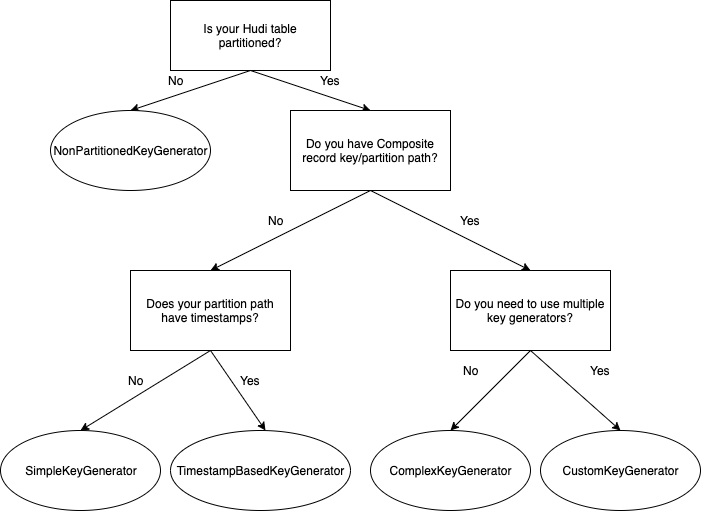
The key generator class can be automatically inferred by Hudi if the specified record key and partition path require a SimpleKeyGenerator or ComplexKeyGenerator, depending on whether there are single or multiple record key or partition path columns. For all other cases, you need to specify the key generator.

The following flow chart explains how to select the right key generator for your use case.

PreCombine field

This is a mandatory field that Hudi uses to deduplicate the records within the same batch before writing them. When two records have the same record key, they go through the preCombine process, and the record with the largest value for the preCombine key is picked by default. This behavior can be customized through custom implementation of the Hudi payload class, which we describe in the next section.

The following table summarizes the configurations related to preCombine.

Configuration Parameter	Description	Value
`hoodie.datasource.write.precombine.field`	The field used in preCombining before the actual write. It helps select the latest record whenever there are multiple updates to the same record in a single incoming data batch.	The default value is ts. You can configure it to any column in your dataset that you want Hudi to use to deduplicate the records whenever there are multiple records with the same record key in the same batch. Currently, you can only pick one field as the preCombine field. Select a column with the timestamp data type or any column that can determine which record holds the latest version, like a monotonically increasing number.
`hoodie.combine.before.upsert`	During upsert, this configuration controls whether deduplication should be done for the incoming batch before ingesting into Hudi. This is applicable only for upsert operations.	The default value is true. We recommend keeping it at the default to avoid duplicates.
`hoodie.combine.before.delete`	Same as the preceding config, but applicable only for delete operations.	The default value is true. We recommend keeping it at the default to avoid duplicates.
`hoodie.combine.before.insert`	When inserted records share the same key, the configuration controls whether they should be first combined (deduplicated) before writing to storage.	The default value is false. We recommend setting it to true if the incoming inserts or bulk inserts can have duplicates.

Record payload

Record payload defines how to merge new incoming records against old stored records for upserts.

The default OverwriteWithLatestAvroPayload payload class always overwrites the stored record with the latest incoming record. This works fine for batch jobs and most use cases. But let’s say you have a streaming job and want to prevent the late-arriving data from overwriting the latest record in storage. You need to use a different payload class implementation (DefaultHoodieRecordPayload) to determine the latest record in storage based on an ordering field, which you provide.

For example, in the following example, Commit 1 has HoodieKey 1, Val 1, preCombine10, and in-flight Commit 2 has HoodieKey 1, Val 2, preCombine 5.

If using the default OverwriteWithLatestAvroPayload, the Val 2 version of the record will be the final version of the record in storage (Amazon S3) because it’s the latest version of the record.

If using DefaultHoodieRecordPayload, it will honor Val 1 because the Val 2’s record version has a lower preCombine value (preCombine 5) compared to Val 1’s record version, while merging multiple versions of the record.

You can select a payload class while writing to the Hudi table using the configuration hoodie.datasource.write.payload.class.

Some useful in-built payload class implementations are described in the following table.

Payload Class	Description
OverwriteWithLatestAvroPayload (`org.apache.hudi.common.model.OverwriteWithLatestAvroPayload`)	Chooses the latest incoming record to overwrite any previous version of the records. Default payload class.
DefaultHoodieRecordPayload (`org.apache.hudi.common.model.DefaultHoodieRecordPayload`)	Uses `hoodie.payload.ordering.field` to determine the final record version while writing to storage.
EmptyHoodieRecordPayload (`org.apache.hudi.common.model.EmptyHoodieRecordPayload`)	Use this as payload class to delete all the records in the dataset.
AWSDmsAvroPayload (`org.apache.hudi.common.model.AWSDmsAvroPayload`)	Use this as payload class if AWS DMS is used as source. It provides support for seamlessly applying changes captured via AWS DMS. This payload implementation performs insert, delete, and update operations on the Hudi table based on the operation type for the CDC record obtained from AWS DMS.

Partitioning

Partitioning is the physical organization of files within a table. They act as virtual columns and can impact the max parallelism we can use on writing.

Extremely fine-grained partitioning (for example, over 20,000 partitions) can create excessive overhead for the Spark engine managing all the small tasks, and can degrade query performance by reducing file sizes. Also, an overly coarse-grained partition strategy, without clustering and data skipping, can negatively impact both read and upsert performance with the need to scan more files in each partition.

Right partitioning helps improve read performance by reducing the amount of data scanned per query. It also improves upsert performance by limiting the number of files scanned to find the file group in which a specific record exists during ingest. A column frequently used in query filters would be a good candidate for partitioning.

For large-scale use cases with evolving query patterns, we suggest coarse-grained partitioning (such as date), while using fine-grained data layout optimization techniques (clustering) within each partition. This opens the possibility of data layout evolution.

By default, Hudi creates the partition folders with just the partition values. We recommend using Hive style partitioning, in which the name of the partition columns is prefixed to the partition values in the path (for example, year=2022/month=07 as opposed to 2022/07). This enables better integration with Hive metastores, such as using msck repair to fix partition paths.

To support Apache Hive style partitions in Hudi, we have to enable it in the config hoodie.datasource.write.hive_style_partitioning.

The following table summarizes the key configurations related to Hudi partitioning.

Configuration Parameter	Description	Value
`hoodie.datasource.write.partitionpath.field`	Partition path field. This is a required configuration that you need to pass while writing the Hudi dataset.	There is no default value set for this. Set it to the column that you have determined for partitioning the data. We recommend that it doesn’t cause extremely fine-grained partitions.
`hoodie.datasource.write.hive_style_partitioning`	Determines whether to use Hive style partitioning. If set to true, the names of partition folders follow `<partition_column_name>=<partition_value>` format.	Default value is false. Set it to true to use Hive style partitioning.
`hoodie.datasource.write.partitionpath.urlencode`	Indicates if we should URL encode the partition path value before creating the folder structure.	Default value is false. Set it to true if you want to URL encode the partition path value. For example, if you’re using the data format “`yyyy-MM-dd HH:mm:ss`“, the URL encode needs to be set to true because it will result in an invalid path due to :.

Note that if the data isn’t partitioned, you need to specifically use NonPartitionedKeyGenerator for the record key, which is explained in the previous section. Additionally, Hudi doesn’t allow partition columns to be changed or evolved.

Choose the right index

After we select the storage type in Hudi and determine the record key and partition path, we need to choose the right index for upsert performance. Apache Hudi employs an index to locate the file group that an update/delete belongs to. This enables efficient upsert and delete operations and enforces uniqueness based on the record keys.

Global index vs. non-global index

When picking the right indexing strategy, the first decision is whether to use a global (table level) or non-global (partition level) index. The main difference between global vs. non-global indexes is the scope of key uniqueness constraints. Global indexes enforce uniqueness of the keys across all partitions of a table. The non-global index implementations enforce this constraint only within a specific partition. Global indexes offer stronger uniqueness guarantees, but they come with a higher update/delete cost, for example global deletes with just the record key need to scan the entire dataset. HBase indexes are an exception here, but come with an operational overhead.

For large-scale global index use cases, use an HBase index or record-level index (available in Hudi 0.13) because for all other global indexes, the update/delete cost grows with the size of the table, O(size of the table).

When using a global index, be aware of the configuration hoodie[bloom|simple|hbase].index.update.partition.path, which is already set to true by default. For existing records getting upserted to a new partition, enabling this configuration will help delete the old record in the old partition and insert it in the new partition.

Hudi index options

After picking the scope of the index, the next step is to decide which indexing option best fits your workload. The following table explains the indexing options available in Hudi as of 0.11.0.

Indexing Option	How It Works	Characteristic	Scope
Simple Index	Performs a join of the incoming upsert/delete records against keys extracted from the involved partition in case of non-global datasets and the entire dataset in case of global or non-partitioned datasets.	Easiest to configure. Suitable for basic use cases like small tables with evenly spread updates. Even for larger tables where updates are very random to all partitions, a simple index is the right choice because it directly joins with interested fields from every data file without any initial pruning, as compared to Bloom, which in the case of random upserts adds additional overhead and doesn’t give enough pruning benefits because the Bloom filters could indicate true positive for most of the files and end up comparing ranges and filters against all these files.	Global/Non-global
Bloom Index (default index in EMR Hudi)	Employs Bloom filters built out of the record keys, optionally also pruning candidate files using record key ranges. Bloom filter is stored in the data file footer while writing the data.	More efficient filter compared to simple index for use cases like late-arriving updates to fact tables and deduplication in event tables with ordered record keys such as timestamp. Hudi implements a dynamic Bloom filter mechanism to reduce false positives provided by Bloom filters. In general, the probability of false positives increases with the number of records in a given file. Check the Hudi FAQ for Bloom filter configuration best practices.	Global/Non-global
Bucket Index	It distributes records to buckets using a hash function based on the record keys or subset of it. It uses the same hash function to determine which file group to match with incoming records. New indexing option since hudi 0.11.0.	Simple to configure. It has better upsert throughput performance compared to the Bloom filter. As of Hudi 0.11.1, only fixed bucket number is supported. This will no longer be an issue with the upcoming consistent hashing bucket index feature, which can dynamically change bucket numbers.	Non-global
HBase Index	The index mapping is managed in an external HBase table.	Best lookup time, especially for large numbers of partitions and files. It comes with additional operational overhead because you need to manage an external HBase table.	Global

Use cases suitable for simple index

Simple indexes are most suitable for workloads with evenly spread updates over partitions and files on small tables, and also for larger tables with dimension kind of workloads because updates are random to all partitions. A common example is a CDC pipeline for a dimension table. In this case, updates end up touching a large number of files and partitions. Therefore, a join with no other pruning is most efficient.

Use cases suitable for Bloom index

Bloom indexes are suitable for most production workloads with uneven update distribution across partitions. For workloads with most updates to recent data like fact tables, Bloom filter rightly fits the bill. It can be clickstream data collected from an ecommerce site, bank transactions in a FinTech application, or CDC logs for a fact table.

When using a Bloom index, be aware of the following configurations:

hoodie.bloom.index.use.metadata – By default, it is set to false. When this flag is on, the Hudi writer gets the index metadata information from the metadata table and doesn’t need to open Parquet file footers to get the Bloom filters and stats. You prune out the files by just using the metadata table and therefore have improved performance for larger tables.
hoodie.bloom.index.prune.by.ranges– Enable or disable range pruning based on use case. By default, it’s already set to true. When this flag is on, range information from files is used to speed up index lookups. This is helpful if the selected record key is monotonously increasing. You can set any record key to be monotonically increasing by adding a timestamp prefix. If the record key is completely random and has no natural ordering (such as UUIDs), it’s better to turn this off, because range pruning will only add extra overhead to the index lookup.

Use cases suitable for bucket index

Bucket indexes are suitable for upsert use cases on huge datasets with a large number of file groups within partitions, relatively even data distribution across partitions, and can achieve relatively even data distribution on the bucket hash field column. It can have better upsert performance in these cases due to no index lookup involved as file groups are located based on a hashing mechanism, which is very fast. This is totally different from both simple and Bloom indexes, where an explicit index lookup step is involved during write. The buckets here has one-one mapping with the hudi file group and since the total number of buckets (defined by hoodie.bucket.index.num.buckets(default – 4)) is fixed here, it can potentially lead to skewed data (data distributed unevenly across buckets) and scalability (buckets can grow over time) issues over time. These issues will be addressed in the upcoming consistent hashing bucket index, which is going to be a special type of bucket index.

Use cases suitable for HBase index

HBase indexes are suitable for use cases where ingestion performance can’t be met using the other index types. These are mostly use cases with global indexes and large numbers of files and partitions. HBase indexes provide the best lookup time but come with large operational overheads if you’re already using HBase for other workloads.

For more information on choosing the right index and indexing strategies for common use cases, refer to Employing the right indexes for fast updates, deletes in Apache Hudi. As you have already seen, Hudi index performance depends heavily on the actual workload. We encourage you to evaluate different indexes for your workload and choose the one which is best suited for your use case.

Migration guidance

With Apache Hudi growing in popularity, one of the fundamental challenges is to efficiently migrate existing datasets to Apache Hudi. Apache Hudi maintains record-level metadata to perform core operations such as upserts and incremental pulls. To take advantage of Hudi’s upsert and incremental processing support, you need to add Hudi record-level metadata to your original dataset.

Using bulk_insert

The recommended way for data migration to Hudi is to perform a full rewrite using bulk_insert. There is no look-up for existing records in bulk_insert and writer optimizations like small file handling. Performing a one-time full rewrite is a good opportunity to write your data in Hudi format with all the metadata and indexes generated and also potentially control file size and sort data by record keys.

You can set the sort mode in a bulk_insert operation using the configuration hoodie.bulkinsert.sort.mode. bulk_insert offers the following sort modes to configure.

Sort Modes	Description
`NONE`	No sorting is done to the records. You can get the fastest performance (comparable to writing parquet files with spark) for initial load with this mode.
`GLOBAL_SORT`	Use this to sort records globally across Spark partitions. It is less performant in initial load than other modes as it repartitions data by partition path and sorts it by record key within each partition. This helps in controlling the number of files generated in the target thereby controlling the target file size. Also, the generated target files will not have overlapping min-max values for record keys which will further help speed up index look-ups during upserts/deletes by pruning out files based on record key ranges in bloom index.
`PARTITION_SORT`	Use this to sort records within Spark partitions. It is more performant for initial load than `Global_Sort` and if your Spark partitions in the data frame are already fairly mapped to the Hudi partitions (dataframe is already repartitioned by partition column), using this mode would be preferred as you can obtain records sorted by record key within each partition.

We recommend to use Global_Sort mode if you can handle the one-time cost. The default sort mode is changed from Global_Sort to None from EMR 6.9 (Hudi 0.12.1). During bulk_insert with Global_Sort, two configurations control the sizes of target files generated by Hudi.

Configuration Parameter	Description	Value
`hoodie.bulkinsert.shuffle.parallelism`	The number of files generated from the bulk insert is determined by this configuration. The higher the parallelism, the more Spark tasks processing the data.	Default value is 200. To control file size and achieve maximum performance (more parallelism), we recommend setting this to a value such that the files generated are equal to the `hoodie.parquet.max.file.size`. If you make parallelism really high, the max file size can’t be honored because the Spark tasks are working on smaller amounts of data.
`hoodie.parquet.max.file.size`	Target size for Parquet files produced by Hudi write phases.	Default value is 120 MB. If the Spark partitions generated with `hoodie.bulkinsert.shuffle.parallelism` are larger than this size, it splits it and generates multiple files to not exceed the max file size.

Let’s say we have a 100 GB Parquet source dataset and we’re bulk inserting with Global_Sort into a partitioned Hudi table with 10 evenly distributed Hudi partitions. We want to have the preferred target file size of 120 MB (default value for hoodie.parquet.max.file.size). The Hudi bulk insert shuffle parallelism should be calculated as follows:

The total data size in MB is 100 * 1024 = 102400 MB
hoodie.bulkinsert.shuffle.parallelism should be set to 102400/120 = ~854

Please note that in reality even with Global_Sort, each spark partition can be mapped to more than one hudi partition and this calculation should only be used as a rough estimate and can potentially end up with more files than the parallelism specified.

Using bootstrapping

For customers operating at scale on hundreds of terabytes or petabytes of data, migrating your datasets to start using Apache Hudi can be time-consuming. Apache Hudi provides a feature called bootstrap to help with this challenge.

The bootstrap operation contains two modes: METADATA_ONLY and FULL_RECORD.

FULL_RECORD is the same as full rewrite, where the original data is copied and rewritten with the metadata as Hudi files.

The METADATA_ONLY mode is the key to accelerating the migration progress. The conceptual idea is to decouple the record-level metadata from the actual data by writing only the metadata columns in the Hudi files generated while the data isn’t copied over and stays in its original location. This significantly reduces the amount of data written, thereby improving the time to migrate and get started with Hudi. However, this comes at the expense of read performance, which involves the overhead merging Hudi files and original data files to get the complete record. Therefore, you may not want to use it for frequently queried partitions.

You can pick and choose these modes at partition level. One common strategy is to tier your data. Use FULL_RECORD mode for a small set of hot partitions, which are accessed frequently, and METADATA_ONLY for a larger set of cold partitions.

Consider the following:

There is some read performance penalty for the METADATA_ONLY partitions, and it should only be used for archived partitions. For more details, refer to Efficient Migration of Large Parquet Tables to Apache Hudi.
The original dataset needs to be in Parquet format to use bootstrap.

Catalog sync

Hudi supports syncing Hudi table partitions and columns to a catalog. On AWS, you can either use the AWS Glue Data Catalog or Hive metastore as the metadata store for your Hudi tables. To register and synchronize the metadata with your regular write pipeline, you need to either enable hive sync or run the hive_sync_tool or AwsGlueCatalogSyncTool command line utility.

We recommend enabling the hive sync feature with your regular write pipeline to make sure the catalog is up to date. If you don’t expect a new partition to be added or the schema changed as part of each batch, then we recommend enabling hoodie.datasource.meta_sync.condition.sync as well so that it allows Hudi to determine if hive sync is necessary for the job.

If you have frequent ingestion jobs and need to maximize ingestion performance, you can disable hive sync and run the hive_sync_tool asynchronously.

If you have the timestamp data type in your Hudi data, we recommend setting hoodie.datasource.hive_sync.support_timestamp to true to convert the int64 (timestamp_micros) to the hive type timestamp. Otherwise, you will see the values in bigint while querying data.

The following table summarizes the configurations related to hive_sync.

Configuration Parameter	Description	Value
`hoodie.datasource.hive_sync.enable`	To register or sync the table to a Hive metastore or the AWS Glue Data Catalog.	Default value is false. We recommend setting the value to true to make sure the catalog is up to date, and it needs to be enabled in every single write to avoid an out-of-sync metastore.
`hoodie.datasource.hive_sync.mode`	This configuration sets the mode for HiveSynctool to connect to the Hive metastore server. For more information, refer to Sync modes.	Valid values are hms, jdbc, and hiveql. If the mode isn’t specified, it defaults to jdbc. Hms and jdbc both talk to the underlying thrift server, but jdbc needs a separate jdbc driver. We recommend setting it to ‘hms’, which uses the Hive metastore client to sync Hudi tables using thrift APIs directly. This helps when using the AWS Glue Data Catalog because you don’t need to install Hive as an application on the EMR cluster (because it doesn’t need the server).
`hoodie.datasource.hive_sync.database`	Name of the destination database that we should sync the Hudi table to.	Default value is default. Set this to the database name of your catalog.
`hoodie.datasource.hive_sync.table`	Name of the destination table that we should sync the Hudi table to.	In Amazon EMR, the value is inferred from the Hudi table name. You can set this config if you need a different table name.
`hoodie.datasource.hive_sync.support_timestamp`	To convert logical type `TIMESTAMP_MICROS` as hive type timestamp.	Default value is false. Set it to true to convert to hive type timestamp.
`hoodie.datasource.meta_sync.condition.sync`	If true, only sync on conditions like schema change or partition change.	Default value is false.

Writing and reading Hudi datasets, and its integration with other AWS services

There are different ways you can write the data to Hudi using Amazon EMR, as explained in the following table.

Hudi Write Options	Description
Spark DataSource	You can use this option to do upsert, insert, or bulk insert for the write operation. Refer to Work with a Hudi dataset for an example of how to write data using DataSourceWrite.
Spark SQL	You can easily write data to Hudi with SQL statements. It eliminates the need to write Scala or PySpark code and adopt a low-code paradigm.
Flink SQL, Flink DataStream API	If you’re using Flink for real-time streaming ingestion, you can use the high-level Flink SQL or Flink DataStream API to write the data to Hudi.
DeltaStreamer	DeltaStreamer is a self-managed tool that supports standard data sources like Apache Kafka, Amazon S3 events, DFS, AWS DMS, JDBC, and SQL sources, built-in checkpoint management, schema validations, as well as lightweight transformations. It can also operate in a continuous mode, in which a single self-contained Spark job can pull data from source, write it out to Hudi tables, and asynchronously perform cleaning, clustering, compactions, and catalog syncing, relying on Spark’s job pools for resource management. It’s easy to use and we recommend using it for all the streaming and ingestion use cases where a low-code approach is preferred. For more information, refer to Streaming Ingestion.
Spark structured streaming	For use cases that require complex data transformations of the source data frame written in Spark DataFrame APIs or advanced SQL, we recommend the structured streaming sink. The streaming source can be used to obtain change feeds out of Hudi tables for streaming or incremental processing use cases.
Kafka Connect Sink	If you standardize on the Apache Kafka Connect framework for your ingestion needs, you can also use the Hudi Connect Sink.

Refer to the following support matrix for query support on specific query engines. The following table explains the different options to read the Hudi dataset using Amazon EMR.

Hudi Read options	Description
Spark DataSource	You can read Hudi datasets directly from Amazon S3 using this option. The tables don’t need to be registered with Hive metastore or the AWS Glue Data Catalog for this option. You can use this option if your use case doesn’t require a metadata catalog. Refer to Work with a Hudi dataset for example of how to read data using DataSourceReadOptions.
Spark SQL	You can query Hudi tables with DML/DDL statements. The tables need to be registered with Hive metastore or the AWS Glue Data Catalog for this option.
Flink SQL	After the Flink Hudi tables have been registered to the Flink catalog, they can be queried using the Flink SQL.
PrestoDB/Trino	The tables need to be registered with Hive metastore or the AWS Glue Data Catalog for this option. This engine is preferred for interactive queries. There is a new Trino connector in upcoming Hudi 0.13, and we recommend reading datasets through this connector when using Trino for performance benefits.
Hive	The tables need to be registered with Hive metastore or the AWS Glue Data Catalog for this option.

Apache Hudi is well integrated with AWS services, and these integrations work when AWS Glue Data Catalog is used, with the exception of Athena, where you can also use a data source connector to an external Hive metastore. The following table summarizes the service integrations.

AWS Service	Description
Amazon Athena	You can use Athena for a serverless option to query a Hudi dataset on Amazon S3. Currently, it supports snapshot queries and read-optimized queries, but not incremental queries. For more details, refer to Using Athena to query Apache Hudi datasets.
Amazon Redshift Spectrum	You can use Amazon Redshift Spectrum to run analytic queries against tables in your Amazon S3 data lake with Hudi format. Currently, it supports only CoW tables. For more details, refer to Creating external tables for data managed in Apache Hudi.
AWS Lake Formation	AWS Lake Formation is used to secure data lakes and define fine-grained access control on the database and table level. Hudi is not currently supported with Amazon EMR Lake Formation integration.
AWS DMS	You can use AWS DMS to ingest data from upstream relational databases to your S3 data lakes into an Hudi dataset. For more details, refer to Apply record level changes from relational databases to Amazon S3 data lake using Apache Hudi on Amazon EMR and AWS Database Migration Service.

Conclusion

This post covered best practices for configuring Apache Hudi data lakes using Amazon EMR. We discussed the key configurations in migrating your existing dataset to Hudi and shared guidance on how to determine the right options for different use cases when setting up Hudi tables.

The upcoming Part 2 of this series focuses on optimizations that can be done on this setup, along with monitoring using Amazon CloudWatch.

About the Authors

Suthan Phillips is a Big Data Architect for Amazon EMR at AWS. He works with customers to provide best practice and technical guidance and helps them achieve highly scalable, reliable and secure solutions for complex applications on Amazon EMR. In his spare time, he enjoys hiking and exploring the Pacific Northwest.

Dylan Qu is an AWS solutions architect responsible for providing architectural guidance across the full AWS stack with a focus on Data Analytics, AI/ML and DevOps.

Automate your Amazon QuickSight deployment with the new API-based account creation and deletion

2022-11-21 Srikanth Baheti

Post Syndicated from Srikanth Baheti original https://aws.amazon.com/blogs/big-data/automate-your-amazon-quicksight-deployment-with-the-new-api-based-account-creation-and-deletion/

Amazon QuickSight is a fully managed, cloud-native business intelligence (BI) service that makes it easy to connect to your data, create interactive dashboards, and share these with tens of thousands of users, either within the QuickSight interface, or embedded in software as a service (SaaS) applications or web portals.

We’re excited to announce the availability of QuickSight APIs that enable administrators and developers to programmatically create and delete accounts with QuickSight Enterprise and Enterprise + Q editions. This allows developers and administrators to automate the deployment and teardown of QuickSight accounts in their organization at scale.

Feature overview

To create and delete QuickSight accounts programmatically, you can use the following APIs:

You need to have the correct AWS Identity and Access Management (IAM) permissions to sign up for QuickSight. For more information, see IAM policy examples for Amazon QuickSight. If your IAM policy includes both the Subscribe and CreateAccountSubscription actions, make sure that both actions are set to Allow. If either action is set to Deny, the Deny action prevails and your API call fails.

Create a QuickSight account

Use the CreateAccountSubscription API to create a QuickSight account:

POST /account/AwsAccountId HTTP/1.1 
Content-type: application/json 
{ 
    "AccountName": "string", 
    "ActiveDirectoryName": "string", 
    "AdminGroup": [ "string" ], 
    "AuthenticationMethod": "string", 
    "AuthorGroup": [ "string" ], 
    "ContactNumber": "string", 
    "DirectoryId": "string", 
    "Edition": "string", 
    "EmailAddress": "string", 
    "FirstName": "string", 
    "LastName": "string", 
    "NotificationEmail": "string", 
    "ReaderGroup": [ "string" ], 
    "Realm": "string" 
}

You can choose to subscribe to Enterprise or Enterprise + Q edition of QuickSight. You can choose the user authentication method: IAM only, IAM and QuickSight, or Active Directory. If you choose Active Directory, you need to provide an Active Directory name and an admin group associated with your Active Directory. Provide the notification email address that you want QuickSight to send notifications to regarding your QuickSight account or QuickSight subscription.

The following code shows the response for CreateAccountSubscription:

HTTP/1.1 Status
Content-type: application/json
{
   "RequestId": "string",
   "SignupResponse": { 
      "accountName": "string",
      "directoryType": "string",
      "IAMUser": boolean,
      "userLoginName": "string"
   }
}

Describe a QuickSight account

Use the DescribeAccountSubscription API to receive a description of a QuickSight account’s subscription:

GET /account/AwsAccountId HTTP/1.1

A successful API call returns an AccountInfo object that includes an account’s name, subscription status, authentication type, edition, and notification email address:

HTTP/1.1 Status 
Content-type: application/json 
{ 
    "AccountInfo": { 
        "AccountName": "string", 
        "AccountSubscriptionStatus": "string", 
        "AuthenticationType": "string", 
        "Edition": "string", 
        "NotificationEmail": "string" 
    },
    "RequestId": "string" 
}

Update and delete a QuickSight account

To avoid accidental deletion, a termination protection flag has been introduced. When a new QuickSight account is provisioned through the CreateAccountSubscription API or user interface, the termination protection flag is set to True by default. You can use the existing DescribeAccountSettings API to inquire the current value of the termination protection flag:

GET /account/AwsAccountId HTTP/1.1

The following code shows the response for DescribeAccountSettings:

HTTP/1.1 Status 
Content-type: application/json
{ 
    "AccountSettings": { 
        "AccountName": "string", 
        "Edition": "string", 
        "DefaultNamespace": "string", 
        "PublicSharingEnabled": "boolean", 
        "NotificationEmail": "string",
        "TerminationProtectionEnabled": "boolean"
    },
    "RequestId": "string" 
}

Use the UpdateAccountSettings API to disable the termination protection flag before proceeding with deleting the account. Optionally, this API can be used to update notification email:

PUT /accounts/{AwsAccountId}/settings HTTP/1.1 
Content-type: application/json 
{ 
    "AwsAccountId": "string", 
    "DefaultNamespace": "string", //Currently only supports default namespace: default 
    "TerminationProtectionEnabled": "boolean",
     "NotificationEmail": "string"
}

After the termination protection has been set to False, use the DeleteAccountSubscription API to delete the QuickSight account:

DELETE /account/{AwsAccountId} HTTP/1.1 
Content-type: application/json

Sample use case

Let’s consider a fictional company, AnyCompany, which owns healthcare facilities across the country. The central IT team of AnyCompany is responsible for setting up and maintaining the IT infrastructure and services for all the facilities in each state. Because AnyCompany is scaling their business, they want to automate the onboarding and maintenance of the IT infrastructure as much as possible. QuickSight is one of the services used by AnyCompany sites, and central IT needs to be able to set up and tear down QuickSight accounts automatically.

The following code shows their sample CreateAccountSubscription API call for setting up a QuickSight Enterprise account:

aws quicksight create-account-subscription --edition ENTERPRISE 
--authentication-method IAM_AND_QUICKSIGHT --aws-account-id XXXXXXXXXXXX 
--account-name quicksight-enterprise-reporting --notification-email XXXXXXXXXX 
--region us-west-2

The following screenshot shows the response.

They use the DescribeAccountSubscription API to monitor the status of new QuickSight account’s subscription:

aws quicksight describe-account-subscription --aws-account-id XXXXXXXXXXX

The following screenshot shows the response.

In case of a site closing event, the following code turns off the account protection using the UpdateAccountSettings API call:

 aws quicksight update-account-settings --aws-account-id XXXXXXXXXXXX 
 --default-namespace default --no-termination-protection-enabled 
 --region us-west-2

The following screenshot shows the response.

The following code deletes the QuickSight account using the DeleteAccountSubscription API call:

aws quicksight delete-account-subscription --aws-account-id XXXXXXXXXXXX 
--region us-west-2

The following screenshot shows the response.

Conclusion

Provisioning and deleting QuickSight accounts enables IT teams to automate their deployments of QuickSight instances across their organization. You can scale and keep up with the rapidly growing business, and minimize human error such as choosing the wrong authentication method. For more information, refer to Amazon QuickSight and What’s New in the Amazon QuickSight User Guide.

Try out QuickSight account provisioning and deletion APIs to automate your QuickSight deployments, and share your feedback and questions in the comments.

About the authors

Srikanth Baheti is a Specialized World Wide Sr. Solution Architect for Amazon QuickSight. He started his career as a consultant and worked for multiple private and government organizations. Later he worked for PerkinElmer Health and Sciences & eResearch Technology Inc, where he was responsible for designing and developing high traffic web applications, highly scalable and maintainable data pipelines for reporting platforms using AWS services and Serverless computing.

Raji Sivasubramaniam is a Sr. Solutions Architect at AWS, focusing on Analytics. Raji is specialized in architecting end-to-end Enterprise Data Management, Business Intelligence and Analytics solutions for Fortune 500 and Fortune 100 companies across the globe. She has in-depth experience in integrated healthcare data and analytics with wide variety of healthcare datasets including managed market, physician targeting and patient analytics.

Mayank Agarwal is a product manager for Amazon QuickSight, AWS’ cloud-native, fully managed BI service. He focuses on account administration, governance and developer experience. He started his career as an embedded software engineer developing handheld devices. Prior to QuickSight he was leading engineering teams at Credence ID, developing custom mobile embedded device and web solutions using AWS services that make biometric enrollment and identification fast, intuitive, and cost-effective for Government sector, healthcare and transaction security applications.

How GoDaddy built a data mesh to decentralize data ownership using AWS Lake Formation

2022-11-21 Ankit Jhalaria

Post Syndicated from Ankit Jhalaria original https://aws.amazon.com/blogs/big-data/how-godaddy-built-a-data-mesh-to-decentralize-data-ownership-using-aws-lake-formation/

This is a guest post co-written with Ankit Jhalaria from GoDaddy.

GoDaddy is empowering everyday entrepreneurs by providing all the help and tools to succeed online. With more than 20 million customers worldwide, GoDaddy is the place people come to name their idea, build a professional website, attract customers, and manage their work.

GoDaddy is a data-driven company, and getting meaningful insights from data helps them drive business decisions to delight their customers. In 2018, GoDaddy began a large infrastructure revamp and partnered with AWS to innovate faster than ever before to meet the needs of its customer growth around the world. As part of this revamp, the GoDaddy Data Platform team wanted to set the company up for long-term success by creating a well-defined data strategy and setting goals to decentralize the ownership and processing of data.

In this post, we discuss how GoDaddy uses AWS Lake Formation to simplify security management and data governance at scale, and enable data as a service (DaaS) supporting organization-wide data accessibility with cross-account data sharing using a data mesh architecture.

The challenge

In the vast ocean of data, deriving useful insights is an art. Prior to the AWS partnership, GoDaddy had a shared Hadoop cluster on premises that various teams used to create and share datasets with other analysts for collaboration. As the teams grew, copies of data started to grow in the Hadoop Distributed File System (HDFS). Several teams started to build tooling to manage this challenge independently, duplicating efforts. Managing permissions on these data assets became harder. Making data discoverable across a growing number of data catalogs and systems is something that had started to become a big challenge. Although the cost of storage these days is relatively inexpensive, when there are several copies of the same data asset available, it makes it harder for analysts to efficiently and reliably use the data available to them. Business analysts need robust pipelines on key datasets that they rely upon to make business decisions.

Solution overview

In GoDaddy’s data mesh hub and spoke model, a central data catalog contains information about all the data products that exist in the company. In AWS terminology, this is the AWS Glue Data Catalog. The data platform team provides APIs, SDKs, and Airflow Operators as components that different teams use to interact with the catalog. Activities such as updating the metastore to reflect a new partition for a given data product, and occasionally running MSCK repair operations, are all handled in the central governance account, and Lake Formation is used to secure access to the Data Catalog.

The data platform team introduced a layer of data governance that ensures best practices for building data products are followed throughout the company. We provide the tooling to support data engineers and business analysts while leaving the domain experts to run their data pipelines. With this approach, we have well-curated data products that are intuitive and easy to understand for our business analysts.

A data product refers to an entity that powers insights for analytical purposes. In simple terms, this could refer to an actual dataset pointing to a location in Amazon Simple Storage Service (Amazon S3). Data producers are responsible for the processing of data and creating new snapshots or partitions depending on the business needs. In some cases, data is refreshed every 24 hours, and other cases, every hour. Data consumers come to the data mesh to consume data, and permissions are managed in the central governance account through Lake Formation. Lake Formation uses AWS Resource Access Manager (AWS RAM) to send resource shares to different consumer accounts to be able to access the data from the central governance account. We go into details about this functionality later in the post.

The following diagram illustrates the solution architecture.

Defining metadata with the central schema repository

Data is only useful if end-users can derive meaningful insights from it—otherwise, it’s just noise. As part of onboarding with the data platform, a data producer registers their schema with the data platform along with relevant metadata. This is reviewed by the data governance team that ensures best practices for creating datasets are followed. We have automated some of the most common data governance review items. This is also the place where producers define a contract about reliable data deliveries, often referred to as Service Level Objective (SLO). After a contract is in place, the data platform team’s background processes monitor and send out alerts when data producers fail to meet their contract or SLO.

When managing permissions with Lake Formation, you register the Amazon S3 location of different S3 buckets. Lake Formation uses AWS RAM to share the named resource.

When managing resources with AWS RAM, the central governance account creates AWS RAM shares. The data platform provides a custom AWS Service Catalog product to accept AWS RAM shares in consumer accounts.

Having consistent schemas with meaningful names and descriptions makes the discovery of datasets easy. Every data producer who is a domain expert is responsible for creating well-defined schemas that business users use to generate insights to make key business decisions. Data producers register their schemas along with additional metadata with the data lake repository. Metadata includes information about the team responsible for the dataset, such as their SLO contract, description, and contact information. This information gets checked into a Git repository where automation kicks in and validates the request to make sure it conforms to standards and best practices. We use AWS CloudFormation templates to provision resources. The following code is a sample of what the registration metadata looks like.

As part of the registration process, automation steps run in the background to take care of the following on behalf of the data producer:

Register the producer’s Amazon S3 location of the data with Lake Formation – This allows us to use Lake Formation for fine-grained access to control the table in the AWS Glue Data Catalog that refers to this location as well as to the underlying data.
Create the underlying AWS Glue database and table – Based on the schema specified by the data producer along with the metadata, we create the underlying AWS Glue database and table in the central governance account. As part of this, we also use table properties of AWS Glue to store additional metadata to use later for analysis.
Define the SLO contract – Any business-critical dataset needs to have a well-defined SLO contract. As part of dataset registration, the data producer defines a contract with a cron expression that gets used by the data platform to create an event rule in Amazon EventBridge. This rule triggers an AWS Lambda function to watch for deliveries of the data and triggers an alert to the data producer’s Slack channel if they breach the contract.

Consuming data from the data mesh catalog

When a data consumer belonging to a given line of business (LOB) identifies the data product that they’re interested in, they submit a request to the central governance team containing their AWS account ID that they use to query the data. The data platform provides a portal to discover datasets across the company. After the request is approved, automation runs to create an AWS RAM share with the consumer account covering the AWS Glue database and tables mapped to the data product registered in the AWS Glue Data Catalog of the central governance account.

The following screenshot shows an example of a resource share.

The consumer data lake admin needs to accept the AWS RAM share and create a resource link in Lake Formation to start querying the shared dataset within their account. We automated this process by building an AWS Service Catalog product that runs in the consumer’s account as a Lambda function that accepts shares on behalf of consumers.

When the resource linked datasets are available in the consumer account, the consumer data lake admin provides grants to IAM users and roles mapping to data consumers within the account. These consumers (application or user persona) can now query the datasets using AWS analytics services of their choice like Amazon Athena and Amazon EMR based on the access privileges granted by the consumer data lake admin.

Day-to-day operations and metrics

Managing permissions using Lake Formation is one part of the overall ecosystem. After permissions have been granted, data producers create new snapshots of the data at a certain cadence that can vary from every 15 minutes to a day. Data producers are integrated with the data platform APIs that informs the platform about any new refreshes of the data. The data platform automatically writes a 0-byte _SUCCESS file for every dataset that gets refreshed, and notifies the subscribed consumer account via an Amazon Simple Notification Service (Amazon SNS) topic in the central governance account. Consumers use this as a signal to trigger their data pipelines and processes to start processing newer version of the data utilizing an event-driven approach.

There are over 2,000 data products built on the GoDaddy data mesh on AWS. Every day, there are thousands of updates to the AWS Glue metastore in the central data governance account. There are hundreds of data producers generating data every hour in a wide array of S3 buckets, and thousands of data consumers consuming data across a wide array of tools, including Athena, Amazon EMR, and Tableau from different AWS accounts.

Business outcomes

With the move to AWS, GoDaddy’s Data Platform team laid the foundations to build a modern data platform that has increased our velocity of building data products and delighting our customers. The data platform has successfully transitioned from a monolithic platform to a model where ownership of data has been decentralized. We accelerated the data platform adoption to over 10 lines of business and over 300 teams globally, and are successfully managing multiple petabytes of data spread across hundreds of accounts to help our business derive insights faster.

Conclusion

GoDaddy’s hub and spoke data mesh architecture built using Lake Formation simplifies security management and data governance at scale, to deliver data as a service supporting company-wide data accessibility. Our data mesh manages multiple petabytes of data across hundreds of accounts, enabling decentralized ownership of well-defined datasets with automation in place, which helps the business discover data assets quicker and derive business insights faster.

This post illustrates the use of Lake Formation to build a data mesh architecture that enables a DaaS model for a modernized enterprise data platform. For more information, see Design a data mesh architecture using AWS Lake Formation and AWS Glue.

About the Authors

Ankit Jhalaria is the Director Of Engineering on the Data Platform at GoDaddy. He has over 10 years of experience working in big data technologies. Outside of work, Ankit loves hiking, playing board games, building IoT projects, and contributing to open-source projects.

Harsh Vardhan is an AWS Solutions Architect, specializing in Analytics. He has over 6 years of experience working in the field of big data and data science. He is passionate about helping customers adopt best practices and discover insights from their data.

Kyle Tedeschi is a Principal Solutions Architect at AWS. He enjoys helping customers innovate, transform, and become leaders in their respective domains. Outside of work, Kyle is an avid snowboarder, car enthusiast, and traveler.

Get started with data integration from Amazon S3 to Amazon Redshift using AWS Glue interactive sessions

2022-11-21 Vikas Omer

Post Syndicated from Vikas Omer original https://aws.amazon.com/blogs/big-data/get-started-with-data-integration-from-amazon-s3-to-amazon-redshift-using-aws-glue-interactive-sessions/

Organizations are placing a high priority on data integration, especially to support analytics, machine learning (ML), business intelligence (BI), and application development initiatives. Data is growing exponentially and is generated by increasingly diverse data sources. Data integration becomes challenging when processing data at scale and the inherent heavy lifting associated with infrastructure required to manage it. This is one of the key reasons why organizations are constantly looking for easy-to-use and low maintenance data integration solutions to move data from one location to another or to consolidate their business data from several sources into a centralized location to make strategic business decisions.

Most organizations use Spark for their big data processing needs. If you’re looking to simplify data integration, and don’t want the hassle of spinning up servers, managing resources, or setting up Spark clusters, we have the solution for you.

AWS Glue is a serverless data integration service that makes it easy to discover, prepare, and combine data for analytics, ML, and application development. AWS Glue provides both visual and code-based interfaces to make data integration simple and accessible for everyone.

If you prefer a code-based experience and want to interactively author data integration jobs, we recommend interactive sessions. Interactive sessions is a recently launched AWS Glue feature that allows you to interactively develop AWS Glue processes, run and test each step, and view the results.

There are different options to use interactive sessions. You can create and work with interactive sessions through the AWS Command Line Interface (AWS CLI) and API. You can also use Jupyter-compatible notebooks to visually author and test your notebook scripts. Interactive sessions provide a Jupyter kernel that integrates almost anywhere that Jupyter does, including integrating with IDEs such as PyCharm, IntelliJ, and Visual Studio Code. This enables you to author code in your local environment and run it seamlessly on the interactive session backend. You can also start a notebook through AWS Glue Studio; all the configuration steps are done for you so that you can explore your data and start developing your job script after only a few seconds. When the code is ready, you can configure, schedule, and monitor job notebooks as AWS Glue jobs.

If you haven’t tried AWS Glue interactive sessions before, this post is highly recommended. We work through a simple scenario where you might need to incrementally load data from Amazon Simple Storage Service (Amazon S3) into Amazon Redshift or transform and enrich your data before loading into Amazon Redshift. In this post, we use interactive sessions within an AWS Glue Studio notebook to load the NYC Taxi dataset into an Amazon Redshift Serverless cluster, query the loaded dataset, save our Jupyter notebook as a job, and schedule it to run using a cron expression. Let’s get started.

Solution overview

We walk you through the following steps:

Set up an AWS Glue Jupyter notebook with interactive sessions.
Use notebook’s magics, including AWS Glue connection and bookmarks.
Read data from Amazon S3, and transform and load it into Redshift Serverless.
Save the notebook as an AWS Glue job and schedule it to run.

Prerequisites

For this walkthrough, we must complete the following prerequisites:

Upload Yellow Taxi Trip Records data and the taxi zone lookup table datasets into Amazon S3. Steps to do that are listed in the next section.
Prepare the necessary AWS Identity and Access Management (IAM) policies and roles to work with AWS Glue Studio Jupyter notebooks, interactive sessions, and AWS Glue.
Create the AWS Glue connection for Redshift Serverless.

Upload datasets into Amazon S3

Download Yellow Taxi Trip Records data and taxi zone lookup table data to your local environment. For this post, we download the January 2022 data for yellow taxi trip records data in Parquet format. The taxi zone lookup data is in CSV format. You can also download the data dictionary for the trip record dataset.

On the Amazon S3 console, create a bucket called my-first-aws-glue-is-project-<random number> in the us-east-1 Region to store the data.S3 bucket names must be unique across all AWS accounts in all the Regions.
Create folders nyc_yellow_taxi and taxi_zone_lookup in the bucket you just created and upload the files you downloaded.
Your folder structures should look like the following screenshots.

Prepare IAM policies and role

Let’s prepare the necessary IAM policies and role to work with AWS Glue Studio Jupyter notebooks and interactive sessions. To get started with notebooks in AWS Glue Studio, refer to Getting started with notebooks in AWS Glue Studio.

Create IAM policies for the AWS Glue notebook role

Create the policy AWSGlueInteractiveSessionPassRolePolicy with the following permissions:

{
    "Version": "2012-10-17",
    "Statement": [
        {
        "Effect": "Allow",
        "Action": "iam:PassRole",
        "Resource":"arn:aws:iam::<AWS account ID>:role/AWSGlueServiceRole-GlueIS"
        }
    ]
}

This policy allows the AWS Glue notebook role to pass to interactive sessions so that the same role can be used in both places. Note that AWSGlueServiceRole-GlueIS is the role that we create for the AWS Glue Studio Jupyter notebook in a later step. Next, create the policy AmazonS3Access-MyFirstGlueISProject with the following permissions:

{
    "Version": "2012-10-17",
    "Statement": [
        {
            "Effect": "Allow",
            "Action": [
                "s3:GetObject",
                "s3:ListBucket"
            ],
            "Resource": [
                "arn:aws:s3:::<your s3 bucket name>",
                "arn:aws:s3:::<your s3 bucket name>/*"
            ]
        }
    ]
}

This policy allows the AWS Glue notebook role to access data in the S3 bucket.

Create an IAM role for the AWS Glue notebook

Create a new AWS Glue role called AWSGlueServiceRole-GlueIS with the following policies attached to it:

Create the AWS Glue connection for Redshift Serverless

Now we’re ready to configure a Redshift Serverless security group to connect with AWS Glue components.

On the Redshift Serverless console, open the workgroup you’re using.
You can find all the namespaces and workgroups on the Redshift Serverless dashboard.
Under Data access, choose Network and security.
Choose the link for the Redshift Serverless VPC security group.You’re redirected to the Amazon Elastic Compute Cloud (Amazon EC2) console.
In the Redshift Serverless security group details, under Inbound rules, choose Edit inbound rules.
Add a self-referencing rule to allow AWS Glue components to communicate:
1. For Type, choose All TCP.
2. For Protocol, choose TCP.
3. For Port range, include all ports.
4. For Source, use the same security group as the group ID.
Similarly, add the following outbound rules:
1. A self-referencing rule with Type as All TCP, Protocol as TCP, Port range including all ports, and Destination as the same security group as the group ID.
2. An HTTPS rule for Amazon S3 access. The s3-prefix-list-id value is required in the security group rule to allow traffic from the VPC to the Amazon S3 VPC endpoint.

If you don’t have an Amazon S3 VPC endpoint, you can create one on the Amazon Virtual Private Cloud (Amazon VPC) console.

You can check the value for s3-prefix-list-id on the Managed prefix lists page on the Amazon VPC console.

Next, go to the Connectors page on AWS Glue Studio and create a new JDBC connection called redshiftServerless to your Redshift Serverless cluster (unless one already exists). You can find the Redshift Serverless endpoint details under your workgroup’s General Information section. The connection setting looks like the following screenshot.

Write interactive code on an AWS Glue Studio Jupyter notebook powered by interactive sessions

Now you can get started with writing interactive code using AWS Glue Studio Jupyter notebook powered by interactive sessions. Note that it’s a good practice to keep saving the notebook at regular intervals while you work through it.

On the AWS Glue Studio console, create a new job.
Select Jupyter Notebook and select Create a new notebook from scratch.
Choose Create.
For Job name, enter a name (for example, myFirstGlueISProject).
For IAM Role, choose the role you created (AWSGlueServiceRole-GlueIS).
Choose Start notebook job.
After the notebook is initialized, you can see some of the available magics and a cell with boilerplate code. To view all the magics of interactive sessions, run %help in a cell to print a full list. With the exception of %%sql, running a cell of only magics doesn’t start a session, but sets the configuration for the session that starts when you run your first cell of code.For this post, we configure AWS Glue with version 3.0, three G.1X workers, idle timeout, and an Amazon Redshift connection with the help of available magics.

Let’s enter the following magics into our first cell and run it:

%glue_version 3.0
%number_of_workers 3
%worker_type G.1X
%idle_timeout 60
%connections redshiftServerless

We get the following response:

Welcome to the Glue Interactive Sessions Kernel
For more information on available magic commands, please type %help in any new cell.

Please view our Getting Started page to access the most up-to-date information on the Interactive Sessions kernel: https://docs.aws.amazon.com/glue/latest/dg/interactive-sessions.html
Installed kernel version: 0.35 
Setting Glue version to: 3.0
Previous number of workers: 5
Setting new number of workers to: 3
Previous worker type: G.1X
Setting new worker type to: G.1X
Current idle_timeout is 2880 minutes.
idle_timeout has been set to 60 minutes.
Connections to be included:
redshiftServerless

Let’s run our first code cell (boilerplate code) to start an interactive notebook session within a few seconds:

import sys
from awsglue.transforms import *
from awsglue.utils import getResolvedOptions
from pyspark.context import SparkContext
from awsglue.context import GlueContext
from awsglue.job import Job
  
sc = SparkContext.getOrCreate()
glueContext = GlueContext(sc)
spark = glueContext.spark_session
job = Job(glueContext)

We get the following response:

Authenticating with environment variables and user-defined glue_role_arn:arn:aws:iam::xxxxxxxxxxxx:role/AWSGlueServiceRole-GlueIS
Attempting to use existing AssumeRole session credentials.
Trying to create a Glue session for the kernel.
Worker Type: G.1X
Number of Workers: 3
Session ID: 7c9eadb1-9f9b-424f-9fba-d0abc57e610d
Applying the following default arguments:
--glue_kernel_version 0.35
--enable-glue-datacatalog true
--job-bookmark-option job-bookmark-enable
Waiting for session 7c9eadb1-9f9b-424f-9fba-d0abc57e610d to get into ready status...
Session 7c9eadb1-9f9b-424f-9fba-d0abc57e610d has been created

Next, read the NYC yellow taxi data from the S3 bucket into an AWS Glue dynamic frame:

nyc_taxi_trip_input_dyf = glueContext.create_dynamic_frame.from_options(
    connection_type = "s3", 
    connection_options = {
        "paths": ["s3://<your-s3-bucket-name>/nyc_yellow_taxi/"]
    }, 
    format = "parquet",
    transformation_ctx = "nyc_taxi_trip_input_dyf"
)

Let’s count the number of rows, look at the schema and a few rows of the dataset.

Count the rows with the following code:

nyc_taxi_trip_input_df = nyc_taxi_trip_input_dyf.toDF()
nyc_taxi_trip_input_df.count()

We get the following response:

View the schema with the following code:

nyc_taxi_trip_input_df.printSchema()

We get the following response:

root
 |-- VendorID: long (nullable = true)
 |-- tpep_pickup_datetime: timestamp (nullable = true)
 |-- tpep_dropoff_datetime: timestamp (nullable = true)
 |-- passenger_count: double (nullable = true)
 |-- trip_distance: double (nullable = true)
 |-- RatecodeID: double (nullable = true)
 |-- store_and_fwd_flag: string (nullable = true)
 |-- PULocationID: long (nullable = true)
 |-- DOLocationID: long (nullable = true)
 |-- payment_type: long (nullable = true)
 |-- fare_amount: double (nullable = true)
 |-- extra: double (nullable = true)
 |-- mta_tax: double (nullable = true)
 |-- tip_amount: double (nullable = true)
 |-- tolls_amount: double (nullable = true)
 |-- improvement_surcharge: double (nullable = true)
 |-- total_amount: double (nullable = true)
 |-- congestion_surcharge: double (nullable = true)
 |-- airport_fee: double (nullable = true)

View a few rows of the dataset with the following code:

nyc_taxi_trip_input_df.show(5)

We get the following response:

+--------+--------------------+---------------------+---------------+-------------+----------+------------------+------------+------------+------------+-----------+-----+-------+----------+------------+---------------------+------------+--------------------+-----------+
|VendorID|tpep_pickup_datetime|tpep_dropoff_datetime|passenger_count|trip_distance|RatecodeID|store_and_fwd_flag|PULocationID|DOLocationID|payment_type|fare_amount|extra|mta_tax|tip_amount|tolls_amount|improvement_surcharge|total_amount|congestion_surcharge|airport_fee|
+--------+--------------------+---------------------+---------------+-------------+----------+------------------+------------+------------+------------+-----------+-----+-------+----------+------------+---------------------+------------+--------------------+-----------+
|       2| 2022-01-18 15:04:43|  2022-01-18 15:12:51|            1.0|         1.13|       1.0|                 N|         141|         229|           2|        7.0|  0.0|    0.5|       0.0|         0.0|                  0.3|        10.3|                 2.5|        0.0|
|       2| 2022-01-18 15:03:28|  2022-01-18 15:15:52|            2.0|         1.36|       1.0|                 N|         237|         142|           1|        9.5|  0.0|    0.5|      2.56|         0.0|                  0.3|       15.36|                 2.5|        0.0|
|       1| 2022-01-06 17:49:22|  2022-01-06 17:57:03|            1.0|          1.1|       1.0|                 N|         161|         229|           2|        7.0|  3.5|    0.5|       0.0|         0.0|                  0.3|        11.3|                 2.5|        0.0|
|       2| 2022-01-09 20:00:55|  2022-01-09 20:04:14|            1.0|         0.56|       1.0|                 N|         230|         230|           1|        4.5|  0.5|    0.5|      1.66|         0.0|                  0.3|        9.96|                 2.5|        0.0|
|       2| 2022-01-24 16:16:53|  2022-01-24 16:31:36|            1.0|         2.02|       1.0|                 N|         163|         234|           1|       10.5|  1.0|    0.5|       3.7|         0.0|                  0.3|        18.5|                 2.5|        0.0|
+--------+--------------------+---------------------+---------------+-------------+----------+------------------+------------+------------+------------+-----------+-----+-------+----------+------------+---------------------+------------+--------------------+-----------+
only showing top 5 rows

Now, read the taxi zone lookup data from the S3 bucket into an AWS Glue dynamic frame:

nyc_taxi_zone_lookup_dyf = glueContext.create_dynamic_frame.from_options(
    connection_type = "s3", 
    connection_options = {
        "paths": ["s3://<your-s3-bucket-name>/taxi_zone_lookup/"]
    }, 
    format = "csv",
    format_options= {
        'withHeader': True
    },
    transformation_ctx = "nyc_taxi_zone_lookup_dyf"
)

Let’s count the number of rows, look at the schema and a few rows of the dataset.

Count the rows with the following code:

nyc_taxi_zone_lookup_df = nyc_taxi_zone_lookup_dyf.toDF()
nyc_taxi_zone_lookup_df.count()

We get the following response:

View the schema with the following code:

nyc_taxi_zone_lookup_apply_mapping_dyf.toDF().printSchema()

We get the following response:

root
 |-- LocationID: string (nullable = true)
 |-- Borough: string (nullable = true)
 |-- Zone: string (nullable = true)
 |-- service_zone: string (nullable = true)

View a few rows with the following code:

nyc_taxi_zone_lookup_df.show(5)

We get the following response:

+----------+-------------+--------------------+------------+
|LocationID|      Borough|                Zone|service_zone|
+----------+-------------+--------------------+------------+
|         1|          EWR|      Newark Airport|         EWR|
|         2|       Queens|         Jamaica Bay|   Boro Zone|
|         3|        Bronx|Allerton/Pelham G...|   Boro Zone|
|         4|    Manhattan|       Alphabet City| Yellow Zone|
|         5|Staten Island|       Arden Heights|   Boro Zone|
+----------+-------------+--------------------+------------+
only showing top 5 rows

Based on the data dictionary, lets recalibrate the data types of attributes in dynamic frames corresponding to both dynamic frames:

nyc_taxi_trip_apply_mapping_dyf = ApplyMapping.apply(
    frame = nyc_taxi_trip_input_dyf, 
    mappings = [
        ("VendorID","Long","VendorID","Integer"), 
        ("tpep_pickup_datetime","Timestamp","tpep_pickup_datetime","Timestamp"), 
        ("tpep_dropoff_datetime","Timestamp","tpep_dropoff_datetime","Timestamp"), 
        ("passenger_count","Double","passenger_count","Integer"), 
        ("trip_distance","Double","trip_distance","Double"),
        ("RatecodeID","Double","RatecodeID","Integer"), 
        ("store_and_fwd_flag","String","store_and_fwd_flag","String"), 
        ("PULocationID","Long","PULocationID","Integer"), 
        ("DOLocationID","Long","DOLocationID","Integer"),
        ("payment_type","Long","payment_type","Integer"), 
        ("fare_amount","Double","fare_amount","Double"),
        ("extra","Double","extra","Double"), 
        ("mta_tax","Double","mta_tax","Double"),
        ("tip_amount","Double","tip_amount","Double"), 
        ("tolls_amount","Double","tolls_amount","Double"), 
        ("improvement_surcharge","Double","improvement_surcharge","Double"), 
        ("total_amount","Double","total_amount","Double"), 
        ("congestion_surcharge","Double","congestion_surcharge","Double"), 
        ("airport_fee","Double","airport_fee","Double")
    ],
    transformation_ctx = "nyc_taxi_trip_apply_mapping_dyf"
)

nyc_taxi_zone_lookup_apply_mapping_dyf = ApplyMapping.apply(
    frame = nyc_taxi_zone_lookup_dyf, 
    mappings = [ 
        ("LocationID","String","LocationID","Integer"), 
        ("Borough","String","Borough","String"), 
        ("Zone","String","Zone","String"), 
        ("service_zone","String", "service_zone","String")
    ],
    transformation_ctx = "nyc_taxi_zone_lookup_apply_mapping_dyf"
)

Now let’s check their schema:

nyc_taxi_trip_apply_mapping_dyf.toDF().printSchema()

We get the following response:

root
 |-- VendorID: integer (nullable = true)
 |-- tpep_pickup_datetime: timestamp (nullable = true)
 |-- tpep_dropoff_datetime: timestamp (nullable = true)
 |-- passenger_count: integer (nullable = true)
 |-- trip_distance: double (nullable = true)
 |-- RatecodeID: integer (nullable = true)
 |-- store_and_fwd_flag: string (nullable = true)
 |-- PULocationID: integer (nullable = true)
 |-- DOLocationID: integer (nullable = true)
 |-- payment_type: integer (nullable = true)
 |-- fare_amount: double (nullable = true)
 |-- extra: double (nullable = true)
 |-- mta_tax: double (nullable = true)
 |-- tip_amount: double (nullable = true)
 |-- tolls_amount: double (nullable = true)
 |-- improvement_surcharge: double (nullable = true)
 |-- total_amount: double (nullable = true)
 |-- congestion_surcharge: double (nullable = true)
 |-- airport_fee: double (nullable = true)

nyc_taxi_zone_lookup_apply_mapping_dyf.toDF().printSchema()

We get the following response:

root
 |-- LocationID: integer (nullable = true)
 |-- Borough: string (nullable = true)
 |-- Zone: string (nullable = true)
 |-- service_zone: string (nullable = true)

Let’s add the column trip_duration to calculate the duration of each trip in minutes to the taxi trip dynamic frame:

# Function to calculate trip duration in minutes
def trip_duration(start_timestamp,end_timestamp):
    minutes_diff = (end_timestamp - start_timestamp).total_seconds() / 60.0
    return(minutes_diff)

# Transformation function for each record
def transformRecord(rec):
    rec["trip_duration"] = trip_duration(rec["tpep_pickup_datetime"], rec["tpep_dropoff_datetime"])
    return rec
nyc_taxi_trip_final_dyf = Map.apply(
    frame = nyc_taxi_trip_apply_mapping_dyf, 
    f = transformRecord, 
    transformation_ctx = "nyc_taxi_trip_final_dyf"
)

Let’s count the number of rows, look at the schema and a few rows of the dataset after applying the above transformation.

Get a record count with the following code:

nyc_taxi_trip_final_df = nyc_taxi_trip_final_dyf.toDF()
nyc_taxi_trip_final_df.count()

We get the following response:

View the schema with the following code:

nyc_taxi_trip_final_df.printSchema()

We get the following response:

root
 |-- extra: double (nullable = true)
 |-- tpep_dropoff_datetime: timestamp (nullable = true)
 |-- trip_duration: double (nullable = true)
 |-- trip_distance: double (nullable = true)
 |-- mta_tax: double (nullable = true)
 |-- improvement_surcharge: double (nullable = true)
 |-- DOLocationID: integer (nullable = true)
 |-- congestion_surcharge: double (nullable = true)
 |-- total_amount: double (nullable = true)
 |-- airport_fee: double (nullable = true)
 |-- payment_type: integer (nullable = true)
 |-- fare_amount: double (nullable = true)
 |-- RatecodeID: integer (nullable = true)
 |-- tpep_pickup_datetime: timestamp (nullable = true)
 |-- VendorID: integer (nullable = true)
 |-- PULocationID: integer (nullable = true)
 |-- tip_amount: double (nullable = true)
 |-- tolls_amount: double (nullable = true)
 |-- store_and_fwd_flag: string (nullable = true)
 |-- passenger_count: integer (nullable = true)

View a few rows with the following code:

nyc_taxi_trip_final_df.show(5)

We get the following response:

+-----+---------------------+------------------+-------------+-------+---------------------+------------+--------------------+------------+-----------+------------+-----------+----------+--------------------+--------+------------+----------+------------+------------------+---------------+
|extra|tpep_dropoff_datetime|     trip_duration|trip_distance|mta_tax|improvement_surcharge|DOLocationID|congestion_surcharge|total_amount|airport_fee|payment_type|fare_amount|RatecodeID|tpep_pickup_datetime|VendorID|PULocationID|tip_amount|tolls_amount|store_and_fwd_flag|passenger_count|
+-----+---------------------+------------------+-------------+-------+---------------------+------------+--------------------+------------+-----------+------------+-----------+----------+--------------------+--------+------------+----------+------------+------------------+---------------+
|  0.0|  2022-01-18 15:12:51| 8.133333333333333|         1.13|    0.5|                  0.3|         229|                 2.5|        10.3|        0.0|           2|        7.0|         1| 2022-01-18 15:04:43|       2|         141|       0.0|         0.0|                 N|              1|
|  0.0|  2022-01-18 15:15:52|              12.4|         1.36|    0.5|                  0.3|         142|                 2.5|       15.36|        0.0|           1|        9.5|         1| 2022-01-18 15:03:28|       2|         237|      2.56|         0.0|                 N|              2|
|  3.5|  2022-01-06 17:57:03| 7.683333333333334|          1.1|    0.5|                  0.3|         229|                 2.5|        11.3|        0.0|           2|        7.0|         1| 2022-01-06 17:49:22|       1|         161|       0.0|         0.0|                 N|              1|
|  0.5|  2022-01-09 20:04:14| 3.316666666666667|         0.56|    0.5|                  0.3|         230|                 2.5|        9.96|        0.0|           1|        4.5|         1| 2022-01-09 20:00:55|       2|         230|      1.66|         0.0|                 N|              1|
|  1.0|  2022-01-24 16:31:36|14.716666666666667|         2.02|    0.5|                  0.3|         234|                 2.5|        18.5|        0.0|           1|       10.5|         1| 2022-01-24 16:16:53|       2|         163|       3.7|         0.0|                 N|              1|
+-----+---------------------+------------------+-------------+-------+---------------------+------------+--------------------+------------+-----------+------------+-----------+----------+--------------------+--------+------------+----------+------------+------------------+---------------+
only showing top 5 rows

Next, load both the dynamic frames into our Amazon Redshift Serverless cluster:

nyc_taxi_trip_sink_dyf = glueContext.write_dynamic_frame.from_jdbc_conf(
    frame = nyc_taxi_trip_final_dyf, 
    catalog_connection = "redshiftServerless", 
    connection_options =  {"dbtable": "public.f_nyc_yellow_taxi_trip","database": "dev"}, 
    redshift_tmp_dir = "s3://aws-glue-assets-<AWS-account-ID>-us-east-1/temporary/", 
    transformation_ctx = "nyc_taxi_trip_sink_dyf"
)

nyc_taxi_zone_lookup_sink_dyf = glueContext.write_dynamic_frame.from_jdbc_conf(
    frame = nyc_taxi_zone_lookup_apply_mapping_dyf, 
    catalog_connection = "redshiftServerless", 
    connection_options = {"dbtable": "public.d_nyc_taxi_zone_lookup", "database": "dev"}, 
    redshift_tmp_dir = "s3://aws-glue-assets-<AWS-account-ID>-us-east-1/temporary/", 
    transformation_ctx = "nyc_taxi_zone_lookup_sink_dyf"
)

Now let’s validate the data loaded in Amazon Redshift Serverless cluster by running a few queries in Amazon Redshift query editor v2. You can also use your preferred query editor.

First, we count the number of records and select a few rows in both the target tables (f_nyc_yellow_taxi_trip and d_nyc_taxi_zone_lookup):
```
SELECT 'f_nyc_yellow_taxi_trip' AS table_name, COUNT(1) FROM "public"."f_nyc_yellow_taxi_trip"
UNION ALL
SELECT 'd_nyc_taxi_zone_lookup' AS table_name, COUNT(1) FROM "public"."d_nyc_taxi_zone_lookup";
```
The number of records in f_nyc_yellow_taxi_trip (2,463,931) and d_nyc_taxi_zone_lookup (265) match the number of records in our input dynamic frame. This validates that all records from files in Amazon S3 have been successfully loaded into Amazon Redshift.

You can view some of the records for each table with the following commands:
```
SELECT * FROM public.f_nyc_yellow_taxi_trip LIMIT 10;
```
```
SELECT * FROM public.d_nyc_taxi_zone_lookup LIMIT 10;
```

One of the insights that we want to generate from the datasets is to get the top five routes with their trip duration. Let’s run the SQL for that on Amazon Redshift:

SELECT 
    CASE WHEN putzl.zone >= dotzl.zone 
        THEN putzl.zone || ' - ' || dotzl.zone 
        ELSE  dotzl.zone || ' - ' || putzl.zone 
    END AS "Route",
    COUNT(1) AS "Frequency",
    ROUND(SUM(trip_duration),1) AS "Total Trip Duration (mins)"
FROM 
    public.f_nyc_yellow_taxi_trip ytt
INNER JOIN 
    public.d_nyc_taxi_zone_lookup putzl ON ytt.pulocationid = putzl.locationid
INNER JOIN 
    public.d_nyc_taxi_zone_lookup dotzl ON ytt.dolocationid = dotzl.locationid
GROUP BY 
    "Route"
ORDER BY 
    "Frequency" DESC, "Total Trip Duration (mins)" DESC
LIMIT 5;

Transform the notebook into an AWS Glue job and schedule it

Now that we have authored the code and tested its functionality, let’s save it as a job and schedule it.

Let’s first enable job bookmarks. Job bookmarks help AWS Glue maintain state information and prevent the reprocessing of old data. With job bookmarks, you can process new data when rerunning on a scheduled interval.

Add the following magic command after the first cell that contains other magic commands initialized during authoring the code:
```
%%configure
{
    "--job-bookmark-option": "job-bookmark-enable"
}
```
To initialize job bookmarks, we run the following code with the name of the job as the default argument (myFirstGlueISProject for this post). Job bookmarks store the states for a job. You should always have job.init() in the beginning of the script and the job.commit() at the end of the script. These two functions are used to initialize the bookmark service and update the state change to the service. Bookmarks won’t work without calling them.

Add the following piece of code after the boilerplate code:

params = []
if '--JOB_NAME' in sys.argv:
    params.append('JOB_NAME')
args = getResolvedOptions(sys.argv, params)
if 'JOB_NAME' in args:
    jobname = args['JOB_NAME']
else:
    jobname = "myFirstGlueISProject"
job.init(jobname, args)

Then comment out all the lines of code that were authored to verify the desired outcome and aren’t necessary for the job to deliver its purpose:

#nyc_taxi_trip_input_df = nyc_taxi_trip_input_dyf.toDF()
#nyc_taxi_trip_input_df.count()
#nyc_taxi_trip_input_df.printSchema()
#nyc_taxi_trip_input_df.show(5)

#nyc_taxi_zone_lookup_df = nyc_taxi_zone_lookup_dyf.toDF()
#nyc_taxi_zone_lookup_df.count()
#nyc_taxi_zone_lookup_df.printSchema()
#nyc_taxi_zone_lookup_df.show(5)

#nyc_taxi_trip_apply_mapping_dyf.toDF().printSchema()
#nyc_taxi_zone_lookup_apply_mapping_dyf.toDF().printSchema()

#nyc_taxi_trip_final_df = nyc_taxi_trip_final_dyf.toDF()
#nyc_taxi_trip_final_df.count()
#nyc_taxi_trip_final_df.printSchema()
#nyc_taxi_trip_final_df.show(5)

Save the notebook.

You can check the corresponding script on the Script tab.Note that job.commit() is automatically added at the end of the script.Let’s run the notebook as a job.
First, truncate f_nyc_yellow_taxi_trip and d_nyc_taxi_zone_lookup tables in Amazon Redshift using the query editor v2 so that we don’t have duplicates in both the tables:
```
truncate "public"."f_nyc_yellow_taxi_trip";
truncate "public"."d_nyc_taxi_zone_lookup";
```
Choose Run to run the job.
You can check its status on the Runs tab.The job completed in less than 5 minutes with G1.x 3 DPUs.
Let’s check the count of records in f_nyc_yellow_taxi_trip and d_nyc_taxi_zone_lookup tables in Amazon Redshift:
```
SELECT 'f_nyc_yellow_taxi_trip' AS table_name, COUNT(1) FROM "public"."f_nyc_yellow_taxi_trip"
UNION ALL
SELECT 'd_nyc_taxi_zone_lookup' AS table_name, COUNT(1) FROM "public"."d_nyc_taxi_zone_lookup";
```
With job bookmarks enabled, even if you run the job again with no new files in corresponding folders in the S3 bucket, it doesn’t process the same files again. The following screenshot shows a subsequent job run in my environment, which completed in less than 2 minutes because there were no new files to process.

Now let’s schedule the job.
On the Schedules tab, choose Create schedule.
For Name¸ enter a name (for example, myFirstGlueISProject-testSchedule).
For Frequency, choose Custom.
Enter a cron expression so the job runs every Monday at 6:00 AM.
Add an optional description.
Choose Create schedule.

The schedule has been saved and activated. You can edit, pause, resume, or delete the schedule from the Actions menu.

Clean up

To avoid incurring future charges, delete the AWS resources you created.

Delete the AWS Glue job (myFirstGlueISProject for this post).
Delete the Amazon S3 objects and bucket (my-first-aws-glue-is-project-<random number> for this post).
Delete the AWS IAM policies and roles (AWSGlueInteractiveSessionPassRolePolicy, AmazonS3Access-MyFirstGlueISProject and AWSGlueServiceRole-GlueIS).
Delete the Amazon Redshift tables (f_nyc_yellow_taxi_trip and d_nyc_taxi_zone_lookup).
Delete the AWS Glue JDBC Connection (redshiftServerless).
Also delete the self-referencing Redshift Serverless security group, and Amazon S3 endpoint (if you created it while following the steps for this post).

Conclusion

In this post, we demonstrated how to do the following:

Set up an AWS Glue Jupyter notebook with interactive sessions
Use the notebook’s magics, including the AWS Glue connection onboarding and bookmarks
Read the data from Amazon S3, and transform and load it into Amazon Redshift Serverless
Configure magics to enable job bookmarks, save the notebook as an AWS Glue job, and schedule it using a cron expression

The goal of this post is to give you step-by-step fundamentals to get you going with AWS Glue Studio Jupyter notebooks and interactive sessions. You can set up an AWS Glue Jupyter notebook in minutes, start an interactive session in seconds, and greatly improve the development experience with AWS Glue jobs. Interactive sessions have a 1-minute billing minimum with cost control features that reduce the cost of developing data preparation applications. You can build and test applications from the environment of your choice, even on your local environment, using the interactive sessions backend.

Interactive sessions provide a faster, cheaper, and more flexible way to build and run data preparation and analytics applications. To learn more about interactive sessions, refer to Job development (interactive sessions), and start exploring a whole new development experience with AWS Glue. Additionally, check out the following posts to walk through more examples of using interactive sessions with different options:

About the Authors

Vikas Omer is a principal analytics specialist solutions architect at Amazon Web Services. Vikas has a strong background in analytics, customer experience management (CEM), and data monetization, with over 13 years of experience in the industry globally. With six AWS Certifications, including Analytics Specialty, he is a trusted analytics advocate to AWS customers and partners. He loves traveling, meeting customers, and helping them become successful in what they do.

Noritaka Sekiyama is a Principal Big Data Architect on the AWS Glue team. He enjoys collaborating with different teams to deliver results like this post. In his spare time, he enjoys playing video games with his family.

Gal Heyne is a Product Manager for AWS Glue and has over 15 years of experience as a product manager, data engineer and data architect. She is passionate about developing a deep understanding of customers’ business needs and collaborating with engineers to design elegant, powerful and easy to use data products. Gal has a Master’s degree in Data Science from UC Berkeley and she enjoys traveling, playing board games and going to music concerts.

Introducing ACK controller for Amazon EMR on EKS

2022-11-19 Peter Dalbhanjan

Post Syndicated from Peter Dalbhanjan original https://aws.amazon.com/blogs/big-data/introducing-ack-controller-for-amazon-emr-on-eks/

AWS Controllers for Kubernetes (ACK) was announced in August, 2020, and now supports 14 AWS service controllers as generally available with an additional 12 in preview. The vision behind this initiative was simple: allow Kubernetes users to use the Kubernetes API to manage the lifecycle of AWS resources such as Amazon Simple Storage Service (Amazon S3) buckets or Amazon Relational Database Service (Amazon RDS) DB instances. For example, you can define an S3 bucket as a custom resource, create this bucket as part of your application deployment, and delete it when your application is retired.

Amazon EMR on EKS is a deployment option for EMR that allows organizations to run Apache Spark on Amazon Elastic Kubernetes Service (Amazon EKS) clusters. With EMR on EKS, the Spark jobs run using the Amazon EMR runtime for Apache Spark. This increases the performance of your Spark jobs so that they run faster and cost less than open source Apache Spark. Also, you can run Amazon EMR-based Apache Spark applications with other types of applications on the same EKS cluster to improve resource utilization and simplify infrastructure management.

Today, we’re excited to announce the ACK controller for Amazon EMR on EKS is generally available. Customers have told us that they like the declarative way of managing Apache Spark applications on EKS clusters. With the ACK controller for EMR on EKS, you can now define and run Amazon EMR jobs directly using the Kubernetes API. This lets you manage EMR on EKS resources directly using Kubernetes-native tools such as kubectl.

The controller pattern has been widely adopted by the Kubernetes community to manage the lifecycle of resources. In fact, Kubernetes has built-in controllers for built-in resources like Jobs or Deployment. These controllers continuously ensure that the observed state of a resource matches the desired state of the resource stored in Kubernetes. For example, if you define a deployment that has NGINX using three replicas, the deployment controller continuously watches and tries to maintain three replicas of NGINX pods. Using the same pattern, the ACK controller for EMR on EKS installs two custom resource definitions (CRDs): VirtualCluster and JobRun. When you create EMR virtual clusters, the controller tracks these as Kubernetes custom resources and calls the EMR on EKS service API (also known as emr-containers) to create and manage these resources. If you want to get a deeper understanding of how ACK works with AWS service APIs, and learn how ACK generates Kubernetes resources like CRDs, see blog post.

If you need a simple getting started tutorial, refer to Run Spark jobs using the ACK EMR on EKS controller. Typically, customers who run Apache Spark jobs on EKS clusters use higher level abstraction such as Argo Workflows, Apache Airflow, or AWS Step Functions, and use workflow-based orchestration in order to run their extract, transform, and load (ETL) jobs. This gives you a consistent experience running jobs while defining job pipelines using Directed Acyclic Graphs (DAGs). DAGs allow you organize your job steps with dependencies and relationships to say how they should run. Argo Workflows is a container-native workflow engine for orchestrating parallel jobs on Kubernetes.

In this post, we show you how to use Argo Workflows with the ACK controller for EMR on EKS to run Apache Spark jobs on EKS clusters.

Solution overview

In the following diagram, we show Argo Workflows submitting a request to the Kubernetes API using its orchestration mechanism.

We’re using Argo to showcase the possibilities with workflow orchestration in this post, but you can also submit jobs directly using kubectl (the Kubernetes command line tool). When Argo Workflows submits these requests to the Kubernetes API, the ACK controller for EMR on EKS reconciles VirtualCluster custom resources by invoking the EMR on EKS APIs.

Let’s go through an exercise of creating custom resources using the ACK controller for EMR on EKS and Argo Workflows.

Prerequisites

Your environment needs the following tools installed:

The AWS Command Line Interface (AWS CLI). For instructions, refer to Installing or updating the latest version of the AWS CLI. The AWS CLI also needs sufficient AWS Identity and Access Management (IAM) permissions to create an EKS cluster.
kubectl, the Kubernetes CLI. For instructions, refer to Install and Set Up kubectl on Linux.
eksctl, the CLI for Amazon EKS. For instructions, see Installing or updating eksctl.
yq, the YAML processor. For more information, refer to the GitHub repo.
Helm 3.7+, the package manager for Kubernetes. For instructions, see Installing Helm.

Install the ACK controller for EMR on EKS

You can either create an EKS cluster or re-use an existing one. We refer to the instructions in Run Spark jobs using the ACK EMR on EKS controller to set up our environment. Complete the following steps:

At this stage, you should have an EKS cluster with proper role-based access control (RBAC) permissions so that Amazon EMR can run its jobs. You should also have the ACK controller for EMR on EKS installed and the EMR job execution role with IAM Roles for Service Account (IRSA) configurations so that they have the correct permissions to call EMR APIs.

Please note, we’re skipping the step to create an EMR virtual cluster because we want to create a custom resource using Argo Workflows. If you created this resource using the getting started tutorial, you can either delete the virtual cluster or create new IAM identity mapping using a different namespace.

Let’s validate the annotation for the EMR on EKS controller service account before proceeding:

# validate annotation
kubectl get pods -n $ACK_SYSTEM_NAMESPACE
CONTROLLER_POD_NAME=$(kubectl get pods -n $ACK_SYSTEM_NAMESPACE --selector=app.kubernetes.io/name=emrcontainers-chart -o jsonpath='{.items..metadata.name}')
kubectl describe pod -n $ACK_SYSTEM_NAMESPACE $CONTROLLER_POD_NAME | grep "^\s*AWS_"

The following code shows the expected results:

AWS_REGION:                      us-west-2
AWS_ENDPOINT_URL:
AWS_ROLE_ARN:                    arn:aws:iam::012345678910:role/ack-emrcontainers-controller
AWS_WEB_IDENTITY_TOKEN_FILE:     /var/run/secrets/eks.amazonaws.com/serviceaccount/token (http://eks.amazonaws.com/serviceaccount/token)

Check the logs of the controller:

kubectl logs ${CONTROLLER_POD_NAME} -n ${ACK_SYSTEM_NAMESPACE}

The following code is the expected outcome:

2022-11-02T18:52:33.588Z    INFO    controller.virtualcluster    Starting Controller    {"reconciler group": "emrcontainers.services.k8s.aws", "reconciler kind": "VirtualCluster"}
2022-11-02T18:52:33.588Z    INFO    controller.virtualcluster    Starting EventSource    {"reconciler group": "emrcontainers.services.k8s.aws", "reconciler kind": "VirtualCluster", "source": "kind source: *v1alpha1.VirtualCluster"}
2022-11-02T18:52:33.589Z    INFO    controller.virtualcluster    Starting Controller    {"reconciler group": "emrcontainers.services.k8s.aws", "reconciler kind": "VirtualCluster"}
2022-11-02T18:52:33.589Z    INFO    controller.jobrun    Starting EventSource    {"reconciler group": "emrcontainers.services.k8s.aws", "reconciler kind": "JobRun", "source": "kind source: *v1alpha1.JobRun"}
2022-11-02T18:52:33.589Z    INFO    controller.jobrun    Starting Controller    {"reconciler group": "emrcontainers.services.k8s.aws", "reconciler kind": "JobRun"}
...
2022-11-02T18:52:33.689Z    INFO    controller.jobrun    Starting workers    {"reconciler group": "emrcontainers.services.k8s.aws", "reconciler kind": "JobRun", "worker count": 1}
2022-11-02T18:52:33.689Z    INFO    controller.virtualcluster    Starting workers    {"reconciler group": "emrcontainers.services.k8s.aws", "reconciler kind": "VirtualCluster", "worker count": 1}

Now we’re ready to install Argo Workflows and use workflow orchestration to create EMR on EKS virtual clusters and submit jobs.

Install Argo Workflows

The following steps are meant for quick installation with a proof of concept in mind. This is not meant for a production install. We recommend reviewing the Argo documentation, security guidelines, and other considerations for a production install.

We install the argo CLI first. We have provided instructions to install the argo CLI using brew, which is compatible with the Mac operating system. If you use Linux or another OS, refer to Quick Start for installation steps.

brew install argo

Let’s create a namespace and install Argo Workflows on your EMR on EKS cluster:

kubectl create namespace argo
kubectl apply -n argo -f https://github.com/argoproj/argo-workflows/releases/download/v3.4.3/install.yaml

You can access the Argo UI locally by port-forwarding the argo-server deployment:

kubectl -n argo port-forward deploy/argo-server 2746:2746

You can access the web UI at https://localhost:2746. You will get a notice that “Your connection is not private” because Argo is using a self-signed certificate. It’s okay to choose Advanced and then Proceed to localhost.

Please note, you get an Access Denied error because we haven’t configured permissions yet. Let’s set up RBAC so that Argo Workflows has permissions to communicate with the Kubernetes API. We give admin permissions to argo serviceaccount in the argo and emr-ns namespaces.

Open another terminal window and run these commands:

# setup rbac 
kubectl create rolebinding default-admin --clusterrole=admin --serviceaccount=argo:default --namespace=argo
kubectl create rolebinding default-admin --clusterrole=admin --serviceaccount=argo:default --namespace=emr-ns

# extract bearer token to login into UI
SECRET=$(kubectl get sa default -n argo -o=jsonpath='{.secrets[0].name}')
ARGO_TOKEN="Bearer $(kubectl get secret $SECRET -n argo -o=jsonpath='{.data.token}' | base64 --decode)"
echo $ARGO_TOKEN

You now have a bearer token that we need to enter for client authentication.

You can now navigate to the Workflows tab and change the namespace to emr-ns to see the workflows under this namespace.

Let’s set up RBAC permissions and create a workflow that creates an EMR on EKS virtual cluster:

cat << EOF > argo-emrcontainers-vc-role.yaml
apiVersion: rbac.authorization.k8s.io/v1
kind: ClusterRole
metadata:
  name: argo-emrcontainers-virtualcluster
rules:
  - apiGroups:
      - emrcontainers.services.k8s.aws
    resources:
      - virtualclusters
    verbs:
      - '*'
EOF

cat << EOF > argo-emrcontainers-jr-role.yaml
apiVersion: rbac.authorization.k8s.io/v1
kind: ClusterRole
metadata:
  name: argo-emrcontainers-jobrun
rules:
  - apiGroups:
      - emrcontainers.services.k8s.aws
    resources:
      - jobruns
    verbs:
      - '*'
EOF

Let’s create these roles and a role binding:

# create argo clusterrole with permissions to emrcontainers.services.k8s.aws
kubectl apply -f argo-emrcontainers-vc-role.yaml
kubectl apply -f argo-emrcontainers-jr-role.yaml

# Give permissions for argo to use emr-containers clusterrole
kubectl create rolebinding argo-emrcontainers-virtualcluster --clusterrole=argo-emrcontainers-virtualcluster --serviceaccount=emr-ns:default -n emr-ns
kubectl create rolebinding argo-emrcontainers-jobrun --clusterrole=argo-emrcontainers-jobrun --serviceaccount=emr-ns:default -n emr-ns

Let’s recap what we have done so far. We created an EMR on EKS cluster, installed the ACK controller for EMR on EKS using Helm, installed the Argo CLI, installed Argo Workflows, gained access to the Argo UI, and set up RBAC permissions for Argo. RBAC permissions are required so that the default service account in the Argo namespace can use VirtualCluster and JobRun custom resources via the emrcontainers.services.k8s.aws API.

It’s time to create the EMR virtual cluster. The environment variables used in the following code are from the getting started guide, but you can change these to meet your environment:

export EKS_CLUSTER_NAME=ack-emr-eks
export EMR_NAMESPACE=emr-ns

cat << EOF > argo-emr-virtualcluster.yaml
apiVersion: argoproj.io/v1alpha1
kind: Workflow
metadata:
  name: emr-virtualcluster
spec:
  arguments: {}
  entrypoint: emr-virtualcluster
  templates:
  - name: emr-virtualcluster
    resource:
      action: create
      manifest: |
        apiVersion: emrcontainers.services.k8s.aws/v1alpha1
        kind: VirtualCluster
        metadata:
          name: my-ack-vc
        spec:
          name: my-ack-vc
          containerProvider:
            id: ${EKS_CLUSTER_NAME}
            type_: EKS
            info:
              eksInfo:
                namespace: ${EMR_NAMESPACE}
EOF

Use the following command to create an Argo Workflow for virtual cluster creation:

kubectl apply -f argo-emr-virtualcluster.yaml -n emr-ns
argo list -n emr-ns

The following code is the expected result from the Argo CLI:

NAME                 STATUS      AGE   DURATION   PRIORITY   MESSAGE
emr-virtualcluster   Succeeded   12m   11s        0

Check the status of virtualcluster:

kubectl describe virtualcluster/my-ack-vc -n emr-ns

The following code is the expected result from the preceding command:

Name:         my-ack-vc
Namespace:    default
Labels:       <none>
Annotations:  <none>
API Version:  emrcontainers.services.k8s.aws/v1alpha1
Kind:         VirtualCluster
...
Status:
  Ack Resource Metadata:
    Arn:               arn:aws:emr-containers:us-west-2:012345678910:/virtualclusters/dxnqujbxexzri28ph1wspbxo0
    Owner Account ID:  012345678910
    Region:            us-west-2
  Conditions:
    Last Transition Time:  2022-11-03T15:34:10Z
    Message:               Resource synced successfully
    Reason:                
    Status:                True
    Type:                  ACK.ResourceSynced
  Id:                      dxnqujbxexzri28ph1wspbxo0
Events:                    <none>

If you run into issues, you can check Argo logs using the following command or through the console:

argo logs emr-virtualcluster -n emr-ns

You can also check controller logs as mentioned in the troubleshooting guide.

Because we have an EMR virtual cluster ready to accept jobs, we can start working on the prerequisites for job submission.

Create an S3 bucket and Amazon CloudWatch Logs group that are needed for the job (see the following code). If you already created these resources from the getting started tutorial, you can skip this step.

export RANDOM_ID1=$(LC_ALL=C tr -dc a-z0-9 </dev/urandom | head -c 8)

aws logs create-log-group --log-group-name=/emr-on-eks-logs/$EKS_CLUSTER_NAME
aws s3 mb s3://$EKS_CLUSTER_NAME-$RANDOM_ID1

We use the New York Citi Bike dataset, which has rider demographics and trip data information. Run the following command to copy the dataset into your S3 bucket:

export S3BUCKET=$EKS_CLUSTER_NAME-$RANDOM_ID1
aws s3 sync s3://tripdata/ s3://${S3BUCKET}/citibike/csv/

Copy the sample Spark application code to your S3 bucket:

aws s3 cp s3://aws-blogs-artifacts-public/artifacts/BDB-2782/citibike-convert-csv-to-parquet.py s3://${S3BUCKET}/application/
aws s3 cp s3://aws-blogs-artifacts-public/artifacts/BDB-2782/citibike-ridership.py s3://${S3BUCKET}/application/
aws s3 cp s3://aws-blogs-artifacts-public/artifacts/BDB-2782/citibike-popular-stations.py s3://${S3BUCKET}/application/
aws s3 cp s3://aws-blogs-artifacts-public/artifacts/BDB-2782/citibike-trips-by-age.py s3://${S3BUCKET}/application/

Now, it’s time to run sample Spark job. Run the following to generate an Argo workflow submission template:

export RANDOM_ID2=$(LC_ALL=C tr -dc a-z0-9 </dev/urandom | head -c 8)

cat << EOF > argo-citibike-steps-jobrun.yaml
apiVersion: argoproj.io/v1alpha1
kind: Workflow
metadata:
  name: emr-citibike-${RANDOM_ID2}
spec:
  entrypoint: emr-citibike
  templates:
  - name: emr-citibike
    steps:
    - - name: emr-citibike-csv-parquet
        template: emr-citibike-csv-parquet
    - - name: emr-citibike-ridership
        template: emr-citibike-ridership
      - name: emr-citibike-popular-stations
        template: emr-citibike-popular-stations
      - name: emr-citibike-trips-by-age
        template: emr-citibike-trips-by-age

  # This is parent job that converts csv data to parquet
  - name: emr-citibike-csv-parquet
    resource:
      action: create
      successCondition: status.state == COMPLETED
      failureCondition: status.state == FAILED      
      manifest: |
        apiVersion: emrcontainers.services.k8s.aws/v1alpha1
        kind: JobRun
        metadata:
          name: my-ack-jobrun-csv-parquet-${RANDOM_ID2}
        spec:
          name: my-ack-jobrun-csv-parquet-${RANDOM_ID2}
          virtualClusterRef:
            from:
              name: my-ack-vc
          executionRoleARN: "${ACK_JOB_EXECUTION_ROLE_ARN}"
          releaseLabel: "emr-6.7.0-latest"
          jobDriver:
            sparkSubmitJobDriver:
              entryPoint: "s3://${S3BUCKET}/application/citibike-convert-csv-to-parquet.py"
              entryPointArguments: [${S3BUCKET}]
              sparkSubmitParameters: "--conf spark.executor.instances=2 --conf spark.executor.memory=1G --conf spark.executor.cores=1 --conf spark.driver.cores=1 --conf spark.sql.shuffle.partitions=60 --conf spark.dynamicAllocation.enabled=false"
          configurationOverrides: |
            ApplicationConfiguration: null
            MonitoringConfiguration:
              CloudWatchMonitoringConfiguration:
                LogGroupName: /emr-on-eks-logs/${EKS_CLUSTER_NAME}
                LogStreamNamePrefix: citibike
              S3MonitoringConfiguration:
                LogUri: s3://${S3BUCKET}/logs

  # This is a child job which runs after csv-parquet jobs is complete
  - name: emr-citibike-ridership
    resource:
      action: create
      manifest: |
        apiVersion: emrcontainers.services.k8s.aws/v1alpha1
        kind: JobRun
        metadata:
          name: my-ack-jobrun-ridership-${RANDOM_ID2}
        spec:
          name: my-ack-jobrun-ridership-${RANDOM_ID2}
          virtualClusterRef:
            from:
              name: my-ack-vc
          executionRoleARN: "${ACK_JOB_EXECUTION_ROLE_ARN}"
          releaseLabel: "emr-6.7.0-latest"
          jobDriver:
            sparkSubmitJobDriver:
              entryPoint: "s3://${S3BUCKET}/application/citibike-ridership.py"
              entryPointArguments: [${S3BUCKET}]
              sparkSubmitParameters: "--conf spark.executor.instances=2 --conf spark.executor.memory=1G --conf spark.executor.cores=1 --conf spark.driver.cores=1 --conf spark.sql.shuffle.partitions=60 --conf spark.dynamicAllocation.enabled=false"
          configurationOverrides: |
            ApplicationConfiguration: null
            MonitoringConfiguration:
              CloudWatchMonitoringConfiguration:
                LogGroupName: /emr-on-eks-logs/${EKS_CLUSTER_NAME}
                LogStreamNamePrefix: citibike
              S3MonitoringConfiguration:
                LogUri: s3://${S3BUCKET}/logs   

  # This is a child job which runs after csv-parquet jobs is complete
  - name: emr-citibike-popular-stations
    resource:
      action: create
      manifest: |
        apiVersion: emrcontainers.services.k8s.aws/v1alpha1
        kind: JobRun
        metadata:
          name: my-ack-jobrun-popular-stations-${RANDOM_ID2}
        spec:
          name: my-ack-jobrun-popular-stations-${RANDOM_ID2}
          virtualClusterRef:
            from:
              name: my-ack-vc
          executionRoleARN: "${ACK_JOB_EXECUTION_ROLE_ARN}"
          releaseLabel: "emr-6.7.0-latest"
          jobDriver:
            sparkSubmitJobDriver:
              entryPoint: "s3://${S3BUCKET}/application/citibike-popular-stations.py"
              entryPointArguments: [${S3BUCKET}]
              sparkSubmitParameters: "--conf spark.executor.instances=2 --conf spark.executor.memory=1G --conf spark.executor.cores=1 --conf spark.driver.cores=1 --conf spark.sql.shuffle.partitions=60 --conf spark.dynamicAllocation.enabled=false"
          configurationOverrides: |
            ApplicationConfiguration: null
            MonitoringConfiguration:
              CloudWatchMonitoringConfiguration:
                LogGroupName: /emr-on-eks-logs/${EKS_CLUSTER_NAME}
                LogStreamNamePrefix: citibike
              S3MonitoringConfiguration:
                LogUri: s3://${S3BUCKET}/logs             

  # This is a child job which runs after csv-parquet jobs is complete
  - name: emr-citibike-trips-by-age
    resource:
      action: create
      manifest: |
        apiVersion: emrcontainers.services.k8s.aws/v1alpha1
        kind: JobRun
        metadata:
          name: my-ack-jobrun-trips-by-age-${RANDOM_ID2}
        spec:
          name: my-ack-jobrun-trips-by-age-${RANDOM_ID2}
          virtualClusterRef:
            from:
              name: my-ack-vc
          executionRoleARN: "${ACK_JOB_EXECUTION_ROLE_ARN}"
          releaseLabel: "emr-6.7.0-latest"
          jobDriver:
            sparkSubmitJobDriver:
              entryPoint: "s3://${S3BUCKET}/application/citibike-trips-by-age.py"
              entryPointArguments: [${S3BUCKET}]
              sparkSubmitParameters: "--conf spark.executor.instances=2 --conf spark.executor.memory=1G --conf spark.executor.cores=1 --conf spark.driver.cores=1 --conf spark.sql.shuffle.partitions=60 --conf spark.dynamicAllocation.enabled=false"
          configurationOverrides: |
            ApplicationConfiguration: null
            MonitoringConfiguration:
              CloudWatchMonitoringConfiguration:
                LogGroupName: /emr-on-eks-logs/${EKS_CLUSTER_NAME}
                LogStreamNamePrefix: citibike
              S3MonitoringConfiguration:
                LogUri: s3://${S3BUCKET}/logs                        
EOF

Let’s run this job:

argo -n emr-ns submit --watch argo-citibike-steps-jobrun.yaml

The following code is the expected result:

Name:                emr-citibike-tp8dlo6c
Namespace:           emr-ns
ServiceAccount:      unset (will run with the default ServiceAccount)
Status:              Succeeded
Conditions:          
 PodRunning          False
 Completed           True
Created:             Mon Nov 07 15:29:34 -0500 (20 seconds ago)
Started:             Mon Nov 07 15:29:34 -0500 (20 seconds ago)
Finished:            Mon Nov 07 15:29:54 -0500 (now)
Duration:            20 seconds
Progress:            4/4
ResourcesDuration:   4s*(1 cpu),4s*(100Mi memory)
STEP                                  TEMPLATE                       PODNAME                                                         DURATION  MESSAGE
 ✔ emr-citibike-if32fvjd              emr-citibike                                                                                               
 ├───✔ emr-citibike-csv-parquet       emr-citibike-csv-parquet       emr-citibike-if32fvjd-emr-citibike-csv-parquet-140307921        2m          
 └─┬─✔ emr-citibike-popular-stations  emr-citibike-popular-stations  emr-citibike-if32fvjd-emr-citibike-popular-stations-1670101609  4s          
   ├─✔ emr-citibike-ridership         emr-citibike-ridership         emr-citibike-if32fvjd-emr-citibike-ridership-2463339702         4s          
   └─✔ emr-citibike-trips-by-age      emr-citibike-trips-by-age      emr-citibike-if32fvjd-emr-citibike-trips-by-age-3778285872      4s

You can open another terminal and run the following command to check on the job status as well:

kubectl -n emr-ns get jobruns -w

You can also check the UI and look at the Argo logs, as shown in the following screenshot.

Clean up

Follow the instructions from the getting started tutorial to clean up the ACK controller for EMR on EKS and its resources. To delete Argo resources, use the following code:

kubectl delete -n argo -f https://github.com/argoproj/argo-workflows/releases/download/v3.4.3/install.yaml
kubectl delete -f argo-emrcontainers-vc-role.yaml
kubectl delete -f argo-emrcontainers-jr-role.yaml
kubectl delete rolebinding argo-emrcontainers-virtualcluster -n emr-ns
kubectl delete rolebinding argo-emrcontainers-jobrun -n emr-ns
kubectl delete ns argo

Conclusion

In this post, we went through how to manage your Spark jobs on EKS clusters using the ACK controller for EMR on EKS. You can define Spark jobs in a declarative fashion and manage these resources using Kubernetes custom resources. We also reviewed how to use Argo Workflows to orchestrate these jobs to get a consistent job submission experience. You can take advantage of the rich features from Argo Workflows such as using DAGs to define multi-step workflows and specify dependencies within job steps, using the UI to visualize and manage the jobs, and defining retries and timeouts at the workflow or task level.

You can get started today by installing the ACK controller for EMR on EKS and start managing your Amazon EMR resources using Kubernetes-native methods.

About the authors

Peter Dalbhanjan is a Solutions Architect for AWS based in Herndon, VA. Peter is passionate about evangelizing and solving complex business problems using combination of AWS services and open source solutions. At AWS, Peter helps with designing and architecting variety of customer workloads.

Amine Hilaly is a Software Development Engineer at Amazon Web Services working on the Kubernetes and Open source related projects for about two years. Amine is a Go, open-source, and Kubernetes fanatic.

Announcing AWS Glue crawler support for Snowflake

2022-11-19 Leonardo Gomez

Post Syndicated from Leonardo Gomez original https://aws.amazon.com/blogs/big-data/announcing-aws-glue-crawler-support-for-snowflake/

For data lake customers who need to discover petabytes of data, AWS Glue crawlers are a popular way to scan data in the background, so you can focus on using the data to make better intelligent decisions. You may also have data in data warehouses such as Snowflake and want the ability to discover the data in the warehouse and combine with data from data lakes to derive insights. AWS Glue crawlers now support Snowflake, making it easier for you to understand updates to Snowflake schema and extract meaningful insights.

To crawl a Snowflake database, you can create and schedule an AWS Glue crawler with an JDBC URL with credential information from AWS Secrets Manager. A configuration option allows you to specify if you want the crawler to crawl the entire database or limit the tables by including the schema or table path and exclude patterns to reduce crawl time. With each run of the crawler, the crawler inspects and catalogs information, such as updates or deletes to Snowflake tables, external tables, views, and materialized views in the AWS Glue Data Catalog. For Snowflake columns with non-Hive compatible types, such as geography or geometry, the crawler extracts that information as a raw data type and makes it available in the Data Catalog.

In this post, we set up an AWS Glue crawler to crawl the OpenStreetMap geospatial dataset, which is freely available through Snowflake Marketplace. This dataset includes all of the OpenStreetMap location data for New York. OpenStreetMap maintains data about businesses, roads, trails, cafes, railway stations, and much more, from all over the world.

Overview of solution

Snowflake is a cloud data platform that provides data solutions from data warehousing to data science. Snowflake Computing is an AWS Advanced Technology Partner with AWS Competencies in Data & Analytics, Machine Learning, and Retail, as well as an AWS service validation for AWS PrivateLink.

In this solution, we use a sample use case involving points of interest in New York City, based on the following Snowflake quick start. Follow sections 1 and 2 to get access to sample geospatial data from Snowflake Marketplace. We show how to interpret the geography data type and understand the different formats. We use the AWS Glue crawler to crawl this OpenStreetMap geospatial dataset and make it available in the Data Catalog with the geography data type maintained where appropriate.

Prerequisites

To follow along, you need the following:

An AWS account.
An AWS Identity and Access Management (IAM) user with access to the following services:
- Amazon Simple Storage Service (Amazon S3)
- AWS Glue
An IAM role with access to run AWS Glue crawlers.
If the AWS account you use to follow this post uses AWS Lake Formation to manage permissions on the AWS Glue Data Catalog, make sure that you log in as a user with access to create databases and tables. For more information, refer to Implicit Lake Formation permissions.
A Snowflake Enterprise Edition account with permission to create storage integrations, ideally in the AWS us-east-1 Region or closest available trial Region, like us-east-2. If necessary, you can subscribe to a Snowflake trial account on AWS Marketplace.
- On the Marketplace listing page, choose Continue to Subscribe, and then choose Accept Terms. You’re redirected to the Snowflake website to begin using the software. To complete your registration, choose Set Up Your Account.
- If you’re new to Snowflake, consider completing the Snowflake in 20 Minutes tutorial. By the end of the tutorial, you should know how to create required Snowflake objects, including warehouses, databases, and tables for storing and querying data.
A Snowflake worksheet (query editor) and associated access to a Snowflake virtual warehouse (compute) and database (storage).
Access to an existing Snowflake account with the ACCOUNTADMIN role or the IMPORT SHARE privilege.

Create an AWS Glue connection to Snowflake

For this post, an AWS Glue connection to your Snowflake cluster is necessary. For more details about how to create it, follow the steps in Performing data transformations using Snowflake and AWS Glue. The following screenshot shows the configuration used to create a connection to the Snowflake cluster for this post.

Create an AWS Glue crawler

To create your crawler, complete the following steps:

On the AWS Glue console, choose Crawlers in the navigation pane.
Choose Create crawler.
For Name, enter a name (for example, glue-blog-snowflake-crawler).
Choose Next.
For Is your data already mapped to Glue tables, select Not yet.
In the Data sources section, choose Add a data source.

For this post, you use a JDBC dataset as a source.

For Data source, choose JDBC.
For Connection, select the connection that you created earlier (for this post, SA-snowflake-connection).
For Include path, enter the path to the Snowflake database you created as a prerequisite (OSM_NEWYORK/NEW_YORK/%).
For Additional metadata, choose COMMENTS and RAWTYPE.

This allows the crawler to harvest metadata related to comments and raw types like geospatial columns.

Choose Add a JDBC data source.

Choose Next.
For Existing IAM role¸ choose the role you created as a prerequisite (for this post, we use AWSGlueServiceRole-DefualtRole).
Choose Next.

Now let’s create an AWS Glue database.

Under Target database, choose Add database.
For Name, enter gluesnowdb.
Choose Create database.
On the Set output and scheduling page, for Target database, choose the database you just created (gluesnowdb).
For Table name prefix, enter blog_.
For Frequency, choose On demand.
Choose Next.
Review the configuration and choose Create crawler.

Run the AWS Glue crawler

To run the crawler, complete the following steps:

On the AWS Glue console, choose Crawlers in the navigation pane.
Choose the crawler you created.
Choose Run crawler.

On the Crawler runs tab, you can see the current run of the crawler.

Wait until the crawler run is complete.

As shown in the following screenshot, 27 tables were added.

Now let’s see how these tables look in the AWS Glue Data Catalog.

Explore the AWS Glue tables

Let’s explore the tables created by the crawler.

On the AWS Glue console, chose Databases in the navigation pane.
Search for and choose the gluesnowdb database.

Now you can see the list of the tables created by the crawler.

Choose the blog_osm_newyork_new_york_v_osm_ny_amenity table.

In the Schema section, you can see that the raw type was also harvested from the source Snowflake database.

Choose the Advanced properties tab.
In the Table properties section, you can see that the classification is snowflake and the typeOfData is view.

Clean up

To avoid incurring future charges, and to clean up unused roles and policies, delete the resources you created: the CloudFormation stack, S3 bucket, AWS Glue crawler, AWS Glue database, and AWS Glue table.

Conclusion

AWS Glue crawlers now support Snowflake tables, views, and materialized views. Offering more options to integrate Snowflake databases to your AWS Glue Data Catalog. You can use AWS Glue crawlers to discover Snowflake datasets, extract schema information, and populate the Data Catalog.

In this post, we provided a procedure to set up AWS Glue crawlers to discover Snowflake tables, which reduces the time and cost needed to incrementally process Snowflake table data updates in the Data Catalog. To learn more about this feature, refer to the docs.

Special thanks to everyone who contributed to this crawler feature launch: Theo Xu, Hunny Vankawala, and Jessica Cheng.

Happy crawling!

Attribution

OpenStreetMap data by OpenStreetMap Foundation is licensed under Open Data Commons Open Database License (ODbL)

About the authors

Leonardo Gómez is a Senior Analytics Specialist Solutions Architect at AWS. Based in Toronto, Canada, he has over a decade of experience in data management, helping customers around the globe address their business and technical needs.

Bosco Albuquerque is a Sr. Partner Solutions Architect at AWS and has over 20 years of experience working with database and analytics products from enterprise database vendors and cloud providers. He has helped technology companies design and implement data analytics solutions and products.

Sandeep Adwankar is a Senior Technical Product Manager at AWS. Based in the California Bay Area, he works with customers around the globe to translate business and technical requirements into products that enable customers to improve how they manage, secure, and access data.

How Cloudflare instruments services using Workers Analytics Engine

2022-11-18 Jen Sells

Post Syndicated from Jen Sells original https://blog.cloudflare.com/using-analytics-engine-to-improve-analytics-engine/

How Cloudflare instruments services using Workers Analytics Engine

Workers Analytics Engine is a new tool, announced earlier this year, that enables developers and product teams to build time series analytics about anything, with high dimensionality, high cardinality, and effortless scaling. We built Analytics Engine for teams to gain insights into their code running in Workers, provide analytics to end customers, or even build usage based billing.

In this blog post we’re going to tell you about how we use Analytics Engine to build Analytics Engine. We’ve instrumented our own Analytics Engine SQL API using Analytics Engine itself and use this data to find bugs and prioritize new product features. We hope this serves as inspiration for other teams who are looking for ways to instrument their own products and gather feedback.

Why do we need Analytics Engine?

Analytics Engine enables you to generate events (or “data points”) from Workers with just a few lines of code. Using the GraphQL or SQL API, you can query these events and create useful insights about the business or technology stack. For more about how to get started using Analytics Engine, check out our developer docs.

Since we released the Analytics Engine open beta in September, we’ve been adding new features at a rapid clip based on feedback from developers. However, we’ve had two big gaps in our visibility into the product.

First, our engineering team needs to answer classic observability questions, such as: how many requests are we getting, how many of those requests result in errors, what are the nature of these errors, etc. They need to be able to view both aggregated data (like average error rate, or p99 response time) and drill into individual events.

Second, because this is a newly launched product, we are looking for product insights. By instrumenting the SQL API, we can understand the queries our customers write, and the errors they see, which helps us prioritize missing features.

We realized that Analytics Engine would be an amazing tool for both answering our technical observability questions, and also gathering product insight. That’s because we can log an event for every query to our SQL API, and then query for both aggregated performance issues as well as individual errors and queries that our customers run.

In the next section, we’re going to walk you through how we use Analytics Engine to monitor that API.

Adding instrumentation to our SQL API

The Analytics Engine SQL API lets you query events data in the same way you would an ordinary database. For decades, SQL has been the most common language for querying data. We wanted to provide an interface that allows you to immediately start asking questions about your data without having to learn a new query language.

Our SQL API parses user SQL queries, transforms and validates them, and then executes them against backend database servers. We then write information about the query back into Analytics Engine so that we can run our own analytics.
Writing data into Analytics Engine from a Cloudflare Worker is very simple and explained in our documentation. We instrument our SQL API in the same way our users do, and this code excerpt shows the data we write into Analytics Engine:

With that data now being stored in Analytics Engine, we can then pull out insights about every field we’re reporting.

Querying for insights

Having our analytics in an SQL database gives you the freedom to write any query you might want. Compared to using something like metrics which are often predefined and purpose specific, you can define any custom dataset desired, and interrogate your data to ask new questions with ease.

We need to support datasets comprising trillions of data points. In order to accomplish this, we have implemented a sampling method called Adaptive Bit Rate (ABR). With ABR, if you have large amounts of data, your queries may be returned sampled events in order to respond in reasonable time. If you have more typical amounts of data, Analytics Engine will query all your data. This allows you to run any query you like and still get responses in a short length of time. Right now, you have to account for sampling in how you make your queries, but we are exploring making it automatic.

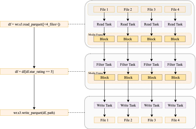
Any data visualization tool can be used to visualize your analytics. At Cloudflare, we heavily use Grafana (and you can too!). This is particularly useful for observability use cases.

Observing query response times

One query we pay attention to gives us information about the performance of our backend database clusters:

As you can see, the 99% percentile (corresponding to the 1% most complex queries to execute) sometimes spikes up to about 300ms. But on average our backend responds to queries within 100ms.

This visualization is itself generated from an SQL query:

Customer insights from high-cardinality data

Another use of Analytics Engine is to draw insights out of customer behavior. Our SQL API is particularly well-suited for this, as you can take full advantage of the power of SQL. Thanks to our ABR technology, even expensive queries can be carried out against huge datasets.

We use this ability to help prioritize improvements to Analytics Engine. Our SQL API supports a fairly standard dialect of SQL but isn’t feature-complete yet. If a user tries to do something unsupported in an SQL query, they get back a structured error message. Those error messages are reported into Analytics Engine. We’re able to aggregate the kinds of errors that our customers encounter, which helps inform which features to prioritize next.

The SQL API returns errors in the format of type of error: more details, and so we can take the first portion before the colon to give us the type of error. We group by that, and get a count of how many times that error happened and how many users it affected:

To perform the above query using an ordinary metrics system, we would need to represent each error type with a different metric. Reporting that many metrics from each microservice creates scalability challenges. That problem doesn’t happen with Analytics Engine, because it’s designed to handle high-cardinality data.

Another big advantage of a high-cardinality store like Analytics Engine is that you can dig into specifics. If there’s a large spike in SQL errors, we may want to find which customers are having a problem in order to help them or identify what function they want to use. That’s easy to do with another SQL query:

Inside Cloudflare, we have historically relied on querying our backend database servers for this type of information. Analytics Engine’s SQL API now enables us to open up our technology to our customers, so they can easily gather insights about their services at any scale!

Conclusion and what’s next

The insights we gathered about usage of the SQL API are a super helpful input to our product prioritization decisions. We already added support for substring and position functions which were used in the visualizations above.

Looking at the top SQL errors, we see numerous errors related to selecting columns. These errors are mostly coming from some usability issues related to the Grafana plugin. Adding support for the DESCRIBE function should alleviate this because without this, the Grafana plugin doesn’t understand the table structure. This, as well as other improvements to our Grafana plugin, is on our roadmap.

We also can see that users are trying to query time ranges for older data that no longer exists. This suggests that our customers would appreciate having extended data retention. We’ve recently extended our retention from 31 to 92 days, and we will keep an eye on this to see if we should offer further extension.

We saw lots of errors related to common mistakes or misunderstandings of proper SQL syntax. This indicates that we could provide better examples or error explanations in our documentation to assist users with troubleshooting their queries.

Stay tuned into our developer docs to be informed as we continue to iterate and add more features!

You can start using Workers Analytics Engine Now! Analytics Engine is now in open beta with free 90-day retention. Start using it today or join our Discord community to talk with the team.

Announcing the AWS Well-Architected Data Analytics Lens

2022-11-17 Dhiraj Thakur

Post Syndicated from Dhiraj Thakur original https://aws.amazon.com/blogs/big-data/announcing-the-aws-well-architected-data-analytics-lens/

We are delighted to announce the release of the Data Analytics Lens. The lens consists of a lens whitepaper and an AWS-created lens available in the Lens Catalog of the AWS Well-Architected Tool. The AWS Well-Architected Framework provides a consistent approach to evaluate architectures and implement scalable designs. With the AWS Well-Architected Framework, cloud architects, system architects, engineers, and developers can build secure, high-performance, resilient, and efficient infrastructure for their applications and workloads.

Using the Lens in the Tool’s Lens Catalog, you can directly assess your Analytics workload in the console, and produce a set of actionable results for customized improvement plans recommended by the Tool.

The updated Data Analytics Lens outlines the most up-to-date steps for performing an AWS Well-Architected review that empowers you to assess and identify technical risks of your data analytics platforms. The new whitepaper and Lens cover multiple analytics use cases and scenarios, and provide comprehensive guidance to help you design your analytics applications in accordance with AWS best practices.

The new Data Analytics Lens offers implementation guidance you can use to deliver secure, high performance and reliable workloads, all with an eye toward maintaining cost-effectiveness and sustainability.

For more information on AWS Well-Architected Lenses, refer to AWS Well-Architected.

What’s new in the Data Analytics Lens?

The Data Analytics Lens is a collection of customer-proven design principles, best practices, and prescriptive guidance to help you adopt a cloud-centered approach to running analytics on AWS. These recommendations are based on insights that AWS has gathered from customers, AWS Partners, the field, and our own analytics technical specialist communities.

This version covers the following topics:

New Lens for the Well-Architected Tool in the Lens Catalog
New Data Mesh analytics user scenario
Included guidance on building ACID compliant data lakes using Iceberg
Included guidance on adding business context to your data catalog to improve searchability and access
How best to leverage Serverless to build sustainable data pipelines
Expanded advanced performance tuning techniques
Additional content for analytics scenario use cases
Links to updated blogs and product documentation, partner solutions, training content, and how-to videos

The lens highlights some of the most common areas for assessment and improvement. It’s designed to align with and provide insights across the six pillars of the AWS Well-Architected Framework:

Operational excellence – Includes the ability to support development and run workloads effectively, gain insight into your operations, and continually improve supporting processes and procedures to deliver business value.
Security – Includes the ability to protect data, systems, and assets to take advantage of cloud technologies to improve your security.
Reliability – Includes the ability of a system to automatically recover from infrastructure or service disruptions, dynamically acquire computing resources to meet demand, and mitigate disruptions such as misconfiguration or transient network issues.
Performance efficiency – Includes the efficient use of computing resources to meet requirements and the maintenance of that efficiency as demand changes and technologies evolve.
Cost optimization – Includes the continual process of system refinement and improvement over the entire lifecycle to optimize cost, from the initial design of your first proof of concept to the ongoing operation of production workloads.
Sustainability – Includes minimizing the environmental impacts of running cloud workloads. Topics including benchmarking, trading data accuracy for carbon, encouraging a data minimization culture, implementing data retention processes, optimizing data modeling, preventing unnecessary data movement, and efficiently managing analytics infrastructure.

The new Data Analytics Lens provides guidance that can help you make appropriate design decisions in line with your business requirements. By applying the techniques detailed in this lens to your architecture, you can validate the resiliency and efficiency of your design. This lens also provides recommendations to address any gaps you may identify.

Who should use the Data Analytics Lens?

The Data Analytics Lens is intended for all AWS customers who use analytics processes to run their workloads.

We believe that the lens will be valuable regardless of your stage of cloud adoption: whether you’re launching your first analytics workloads on AWS, migrating existing services to the cloud, or working to extend and improve existing AWS analytics workloads.

The material is intended to support customers in roles such as architects, developers, and operations team members.

Conclusion

Applying the Data Analytics Lens to your existing architectures can validate the stability and efficiency of your design and provide recommendations to address identified gaps.

For more information about building your own Well-Architected systems using the Data Analytics Lens, see the Data Analytics Lens whitepaper. For information about on the new Lens, please see the Well Architected Tool and Lens Catalog briefs. If you require additional expert guidance, contact your AWS account team to engage a Specialist Solutions Architect.

To learn more about supported analytics solutions, customer case studies, and additional resources, refer to Architecture Best Practices for Analytics & Big Data.

About the authors

Russell Jackson is a Senior Solutions Architect at AWS based in the UK. Russell has over 15 years of analytics experience and is passionate about Big Data, event driven-architectures and building environmentally sustainable data pipelines. Outside of work, Russell enjoys road cycling, wild swimming and traveling.

Theo Tolv is a Senior Analytics Architect based in Stockholm, Sweden. He’s worked with small and big data for most of his career, and has built applications running on AWS since 2008. In his spare time he likes to tinker with electronics and read space opera.

Bruce Ross is a Senior Solutions Architect at AWS in the New York Area. Bruce is the Lens Leader for the Well-Architected Framework. He has been involved in IT and Content Development for over 20 years. He is an avid sailor and angler, and enjoys R&B, jazz, and classical music.

Dhiraj Thakur is a Solutions Architect with Amazon Web Services. He works with AWS customers and partners to provide guidance on enterprise cloud adoption, migration, and strategy. He is passionate about technology and enjoys building and experimenting in the analytics and AI/ML space.

Pragnesh Shah is a Solutions Architect in the Partner Organisation. He is specialist in migration, modernisation, Cloud strategy, designing and delivering data and analytics capabilities. Outside of work, he spends time with family and nature. He likes to record nature sound and practice Zen meditation.

Share and publish your Snowflake data to AWS Data Exchange using Amazon Redshift data sharing

2022-11-17 Raks Khare

Post Syndicated from Raks Khare original https://aws.amazon.com/blogs/big-data/share-and-publish-your-snowflake-data-to-aws-data-exchange-using-amazon-redshift-data-sharing/

Amazon Redshift is a fully managed, petabyte-scale data warehouse service in the cloud. You can start with just a few hundred gigabytes of data and scale to a petabyte or more. Today, tens of thousands of AWS customers—from Fortune 500 companies, startups, and everything in between—use Amazon Redshift to run mission-critical business intelligence (BI) dashboards, analyze real-time streaming data, and run predictive analytics. With the constant increase in generated data, Amazon Redshift customers continue to achieve successes in delivering better service to their end-users, improving their products, and running an efficient and effective business.

In this post, we discuss a customer who is currently using Snowflake to store analytics data. The customer needs to offer this data to clients who are using Amazon Redshift via AWS Data Exchange, the world’s most comprehensive service for third-party datasets. We explain in detail how to implement a fully integrated process that will automatically ingest data from Snowflake into Amazon Redshift and offer it to clients via AWS Data Exchange.

Overview of the solution

The solution consists of four high-level steps:

Configure Snowflake to push the changed data for identified tables into an Amazon Simple Storage Service (Amazon S3) bucket.
Use a custom-built Redshift Auto Loader to load this Amazon S3 landed data to Amazon Redshift.
Merge the data from the change data capture (CDC) S3 staging tables to Amazon Redshift tables.
Use Amazon Redshift data sharing to license the data to customers via AWS Data Exchange as a public or private offering.

The following diagram illustrates this workflow.

Prerequisites

To get started, you need the following prerequisites:

A Snowflake account in the same Region as your Amazon Redshift cluster.
An S3 bucket. Refer to Create your first S3 bucket for more details.
An Amazon Redshift cluster with encryption enabled and an AWS Identity and Access Management (IAM) role with permission to the S3 bucket. See Create a sample Amazon Redshift cluster and Create an IAM role for Amazon Redshift for more details.
A database schema from Snowflake to Amazon Redshift that is migrated using the AWS Schema Conversion Tool (AWS SCT). For more information, refer to Accelerate Snowflake to Amazon Redshift migration using AWS Schema Conversion Tool.
An IAM role and external Amazon S3 stage for Snowflake access to the S3 bucket you created earlier. For instructions, refer to Configuring Secure Access to Amazon S3. Name this external stage unload_to_s3, pointing to the s3-redshift-loader-source folder of the target S3 bucket. It will be referenced in COPY commands later in this post for offloading the data to Amazon S3. Once created, you should see an external stage created as shown in the following screenshot.
You must be a registered provider on AWS Data Exchange. For more information, see Providing data products on AWS Data Exchange.

Configure Snowflake to track the changed data and unload it to Amazon S3

In Snowflake, identify the tables that you need to replicate to Amazon Redshift. For the purpose of this demo, we use the data in the TPCH_SF1 schema’s Customer, LineItem, and Orders tables of the SNOWFLAKE_SAMPLE_DATA database, which comes out of the box with your Snowflake account.

Make sure that the Snowflake external stage name unload_to_s3 created in the prerequisites is pointing to the S3 prefix s3-redshift-loader-sourcecreated in the previous step.
Create a new schema BLOG_DEMO in the DEMO_DB database:CREATE SCHEMA demo_db.blog_demo;

Duplicate the Customer, LineItem, and Orders tables in the TPCH_SF1 schema to the BLOG_DEMO schema:

CREATE TABLE CUSTOMER AS 
SELECT * FROM snowflake_sample_data.tpch_sf1.CUSTOMER;
CREATE TABLE ORDERS AS
SELECT * FROM snowflake_sample_data.tpch_sf1.ORDERS;
CREATE TABLE LINEITEM AS 
SELECT * FROM snowflake_sample_data.tpch_sf1.LINEITEM;

Verify that the tables have been duplicated successfully:

SELECT table_catalog, table_schema, table_name, row_count, bytes
FROM INFORMATION_SCHEMA.TABLES
WHERE TABLE_SCHEMA = 'BLOG_DEMO'
ORDER BY ROW_COUNT;

unload-step-4

Create table streams to track data manipulation language (DML) changes made to the tables, including inserts, updates, and deletes:

CREATE OR REPLACE STREAM CUSTOMER_CHECK ON TABLE CUSTOMER;
CREATE OR REPLACE STREAM ORDERS_CHECK ON TABLE ORDERS;
CREATE OR REPLACE STREAM LINEITEM_CHECK ON TABLE LINEITEM;

Perform DML changes to the tables (for this post, we run UPDATE on all tables and MERGE on the customer table):

UPDATE customer 
SET c_comment = 'Sample comment for blog demo' 
WHERE c_custkey between 0 and 10; 
UPDATE orders 
SET o_comment = 'Sample comment for blog demo' 
WHERE o_orderkey between 1800001 and 1800010; 
UPDATE lineitem 
SET l_comment = 'Sample comment for blog demo' 
WHERE l_orderkey between 3600001 and 3600010;

MERGE INTO customer c 
USING 
( 
SELECT n_nationkey 
FROM snowflake_sample_data.tpch_sf1.nation s 
WHERE n_name = 'UNITED STATES') n 
ON n.n_nationkey = c.c_nationkey 
WHEN MATCHED THEN UPDATE SET c.c_comment = 'This is US based customer1';

Validate that the stream tables have recorded all changes:
```
SELECT * FROM CUSTOMER_CHECK; 
SELECT * FROM ORDERS_CHECK; 
SELECT * FROM LINEITEM_CHECK;
```
For example, we can query the following customer key value to verify how the events were recorded for the MERGE statement on the customer table:

SELECT * FROM CUSTOMER_CHECK where c_custkey = 60027;

We can see the METADATA$ISUPDATE column as TRUE, and we see DELETE followed by INSERT in the METADATA$ACTION column.

Run the COPY command to offload the CDC from the stream tables to the S3 bucket using the external stage name unload_to_s3.In the following code, we’re also copying the data to S3 folders ending with _stg to ensure that when Redshift Auto Loader automatically creates these tables in Amazon Redshift, they get created and marked as staging tables:

COPY INTO @unload_to_s3/customer_stg/
FROM (select *, sysdate() as LAST_UPDATED_TS from demo_db.blog_demo.customer_check)
FILE_FORMAT = (TYPE = PARQUET)
OVERWRITE = TRUE HEADER = TRUE;

COPY INTO @unload_to_s3/customer_stg/
FROM (select *, sysdate() as LAST_UPDATED_TS from demo_db.blog_demo.customer_check)
FILE_FORMAT = (TYPE = PARQUET)
OVERWRITE = TRUE HEADER = TRUE;

COPY INTO @unload_to_s3/lineitem_stg/ 
FROM (select *, sysdate() as LAST_UPDATED_TS from demo_db.blog_demo.lineitem_check) 
FILE_FORMAT = (TYPE = PARQUET) 
OVERWRITE = TRUE HEADER = TRUE;

Verify the data in the S3 bucket. There will be three sub-folders created in the s3-redshift-loader-source folder of the S3 bucket, and each will have .parquet data files.You can also automate the preceding COPY commands using tasks, which can be scheduled to run at a set frequency for automatic copy of CDC data from Snowflake to Amazon S3.
Use the ACCOUNTADMIN role to assign the EXECUTE TASK privilege. In this scenario, we’re assigning the privileges to the SYSADMIN role:
```
USE ROLE accountadmin;
GRANT EXECUTE TASK, EXECUTE MANAGED TASK ON ACCOUNT TO ROLE sysadmin;
```

Use the SYSADMIN role to create three separate tasks to run three COPY commands every 5 minutes: USE ROLE sysadmin;

/* Task to offload Customer CDC table */ 
CREATE TASK sf_rs_customer_cdc 
WAREHOUSE = SMALL 
SCHEDULE = 'USING CRON 5 * * * * UTC' 
AS 
COPY INTO @unload_to_s3/customer_stg/ 
FROM (select *, sysdate() as LAST_UPDATED_TS from demo_db.blog_demo.customer_check) 
FILE_FORMAT = (TYPE = PARQUET) 
OVERWRITE = TRUE 
HEADER = TRUE;

/*Task to offload Orders CDC table */ 
CREATE TASK sf_rs_orders_cdc 
WAREHOUSE = SMALL 
SCHEDULE = 'USING CRON 5 * * * * UTC' 
AS 
COPY INTO @unload_to_s3/orders_stg/ 
FROM (select *, sysdate() as LAST_UPDATED_TS from demo_db.blog_demo.orders_check)
FILE_FORMAT = (TYPE = PARQUET)
OVERWRITE = TRUE HEADER = TRUE;

/* Task to offload Lineitem CDC table */ 
CREATE TASK sf_rs_lineitem_cdc 
WAREHOUSE = SMALL 
SCHEDULE = 'USING CRON 5 * * * * UTC' 
AS 
COPY INTO @unload_to_s3/lineitem_stg/ 
FROM (select *, sysdate() as LAST_UPDATED_TS from demo_db.blog_demo.lineitem_check)
FILE_FORMAT = (TYPE = PARQUET)
OVERWRITE = TRUE HEADER = TRUE;

When the tasks are first created, they’re in a SUSPENDED state.

Alter the three tasks and set them to RESUME state:

ALTER TASK sf_rs_customer_cdc RESUME;
ALTER TASK sf_rs_orders_cdc RESUME;
ALTER TASK sf_rs_lineitem_cdc RESUME;

Validate that all three tasks have been resumed successfully: SHOW TASKS;Now the tasks will run every 5 minutes and look for new data in the stream tables to offload to Amazon S3.As soon as data is migrated from Snowflake to Amazon S3, Redshift Auto Loader automatically infers the schema and instantly creates corresponding tables in Amazon Redshift. Then, by default, it starts loading data from Amazon S3 to Amazon Redshift every 5 minutes. You can also change the default setting of 5 minutes.
On the Amazon Redshift console, launch the query editor v2 and connect to your Amazon Redshift cluster.
Browse to the dev database, public schema, and expand Tables.
You can see three staging tables created with the same name as the corresponding folders in Amazon S3.
Validate the data in one of the tables by running the following query:SELECT * FROM "dev"."public"."customer_stg";

Configure the Redshift Auto Loader utility

The Redshift Auto Loader makes data ingestion to Amazon Redshift significantly easier because it automatically loads data files from Amazon S3 to Amazon Redshift. The files are mapped to the respective tables by simply dropping files into preconfigured locations on Amazon S3. For more details about the architecture and internal workflow, refer to the GitHub repo.

We use an AWS CloudFormation template to set up Redshift Auto Loader. Complete the following steps:

Launch the CloudFormation template.
Choose Next.
For Stack name, enter a name.

Provide the parameters listed in the following table.

CloudFormation Template Parameter	Allowed Values	Description
`RedshiftClusterIdentifier`	Amazon Redshift cluster identifier	Enter the Amazon Redshift cluster identifier.
`DatabaseUserName`	Database user name in the Amazon Redshift cluster	The Amazon Redshift database user name that has access to run the SQL script.
`DatabaseName`	S3 bucket name	The name of the Amazon Redshift primary database where the SQL script is run.
`DatabaseSchemaName`	Database name in Amazon Redshift	The Amazon Redshift schema name where the tables are created.
`RedshiftIAMRoleARN`	Default or the valid IAM role ARN attached to the Amazon Redshift cluster	The IAM role ARN associated with the Amazon Redshift cluster. Your default IAM role is set for the cluster and has access to your S3 bucket, leave it at the default.
`CopyCommandOptions`	Copy option; default is delimiter ‘\|’ gzip	Provide the additional COPY command data format parameters. If InitiateSchemaDetection = Yes, then the process attempts to detect the schema and automatically set the suitable copy command options. In the event of failure on schema detection or when InitiateSchemaDetection = No, then this value is used as the default COPY command options to load data.
`SourceS3Bucket`	S3 bucket name	The S3 bucket where the data is stored. Make sure the IAM role that is associated to the Amazon Redshift cluster has access to this bucket.
`InitiateSchemaDetection`	Yes/No	Set to Yes to dynamically detect the schema prior to file load and create a table in Amazon Redshift if it doesn’t exist already. If a table already exists, then it won’t drop or recreate the table in Amazon Redshift. If schema detection fails, the process uses the default COPY options as specified in `CopyCommandOptions`.

The Redshift Auto Loader uses the COPY command to load data into Amazon Redshift. For this post, set CopyCommandOptions as follows, and configure any supported COPY command options:

delimiter '|' dateformat 'auto' TIMEFORMAT 'auto'

autoloader-input-parameters

Choose Next.
Accept the default values on the next page and choose Next.
Select the acknowledgement check box and choose Create stack.
Monitor the progress of the Stack creation and wait until it is complete.
To verify the Redshift Auto Loader configuration, sign in to the Amazon S3 console and navigate to the S3 bucket you provided.
You should see a new directory s3-redshift-loader-source is created.

Copy all the data files exported from Snowflake under s3-redshift-loader-source.

Merge the data from the CDC S3 staging tables to Amazon Redshift tables

To merge your data from Amazon S3 to Amazon Redshift, complete the following steps:

Create a temporary staging table merge_stg and insert all the rows from the S3 staging table that have metadata_action as INSERT, using the following code. This includes all the new inserts as well as the update.
```
CREATE TEMP TABLE merge_stg 
AS
SELECT * FROM
(
SELECT *, DENSE_RANK() OVER (PARTITION BY c_custkey ORDER BY last_updated_ts DESC
) AS rnk
FROM customer_stg WHERE rnk = 1 AND metadata$action = 'INSERT'
```
The preceding code uses a window function DENSE_RANK() to select the latest entries for a given c_custkey by assigning a rank to each row for a given c_custkey and arrange the data in descending order using last_updated_ts. We then select the rows with rnk=1 and metadata$action = ‘INSERT’ to capture all the inserts.
Use the S3 staging table customer_stg to delete the records from the base table customer, which are marked as deletes or updates:
```
DELETE FROM customer 
USING customer_stg 
WHERE customer.c_custkey = customer_stg.c_custkey;
```
This deletes all the rows that are present in the CDC S3 staging table, which takes care of rows marked for deletion and updates.

Use the temporary staging table merge_stg to insert the records marked for updates or inserts:

INSERT INTO customer 
SELECT c_custkey, c_name, c_address, c_nationkey, c_phone, c_acctbal, c_mktsegment, c_comment 
FROM merge_stg;

Truncate the staging table, because we have already updated the target table:truncate customer_stg;

You can also run the preceding steps as a stored procedure:

CREATE OR REPLACE PROCEDURE merge_customer()
AS $$
BEGIN
/*CREATING TEMP TABLE TO GET THE MOST LATEST RECORDS FOR UPDATES/NEW INSERTS*/
CREATE TEMP TABLE merge_stg AS
SELECT * FROM
(
SELECT *, DENSE_RANK() OVER (PARTITION BY c_custkey ORDER BY last_updated_ts DESC ) AS rnk
FROM customer_stg
)
WHERE rnk = 1 AND metadata$action = 'INSERT';
/* DELETING FROM THE BASE TABLE USING THE CDC STAGING TABLE ALL THE RECORDS MARKED AS DELETES OR UPDATES*/
DELETE FROM customer
USING customer_stg
WHERE customer.c_custkey = customer_stg.c_custkey;
/*INSERTING NEW/UPDATED RECORDS IN THE BASE TABLE*/ 
INSERT INTO customer
SELECT c_custkey, c_name, c_address, c_nationkey, c_phone, c_acctbal, c_mktsegment, c_comment
FROM merge_stg;
truncate customer_stg;
END;
$$ LANGUAGE plpgsql;

For example, let’s look at the before and after states of the customer table when there’s been a change in data for a particular customer.

The following screenshot shows the new changes recorded in the customer_stg table for c_custkey = 74360.
merge-process-new-changes
We can see two records for a customer with c_custkey=74360 one with metadata$action as DELETE and one with metadata$action as INSERT. That means the record with c_custkey was updated at the source and these changes need to be applied to the target customer table in Amazon Redshift.

The following screenshot shows the current state of the customer table before these changes have been merged using the preceding stored procedure:
merge-process-current-state

Now, to update the target table, we can run the stored procedure as follows: CALL merge_customer()The following screenshot shows the final state of the target table after the stored procedure is complete.

Run the stored procedure on a schedule

You can also run the stored procedure on a schedule via Amazon EventBridge. The scheduling steps are as follows:

On the EventBridge console, choose Create rule.
For Name, enter a meaningful name, for example, Trigger-Snowflake-Redshift-CDC-Merge.
For Event bus, choose default.
For Rule Type, select Schedule.
Choose Next.
For Schedule pattern, select A schedule that runs at a regular rate, such as every 10 minutes.
For Rate expression, enter Value as 5 and choose Unit as Minutes.
Choose Next.
For Target types, choose AWS service.
For Select a Target, choose Redshift cluster.
For Cluster, choose the Amazon Redshift cluster identifier.
For Database name, choose dev.
For Database user, enter a user name with access to run the stored procedure. It uses temporary credentials to authenticate.
Optionally, you can also use AWS Secrets Manager for authentication.
For SQL statement, enter CALL merge_customer().
For Execution role, select Create a new role for this specific resource.
Choose Next.
Review the rule parameters and choose Create rule.

After the rule has been created, it automatically triggers the stored procedure in Amazon Redshift every 5 minutes to merge the CDC data into the target table.

Configure Amazon Redshift to share the identified data with AWS Data Exchange

Now that you have the data stored inside Amazon Redshift, you can publish it to customers using AWS Data Exchange.

In Amazon Redshift, using any query editor, create the data share and add the tables to be shared:

CREATE DATASHARE salesshare MANAGEDBY ADX;
ALTER DATASHARE salesshare ADD SCHEMA tpch_sf1;
ALTER DATASHARE salesshare ADD TABLE tpch_sf1.customer;

ADX-step1

On the AWS Data Exchange console, create your dataset.
Select Amazon Redshift datashare.
Create a revision in the dataset.
Add assets to the revision (in this case, the Amazon Redshift data share).
Finalize the revision.

After you create the dataset, you can publish it to the public catalog or directly to customers as a private product. For instructions on how to create and publish products, refer to NEW – AWS Data Exchange for Amazon Redshift

Clean up

To avoid incurring future charges, complete the following steps:

Delete the CloudFormation stack used to create the Redshift Auto Loader.
Delete the Amazon Redshift cluster created for this demonstration.
If you were using an existing cluster, drop the created external table and external schema.
Delete the S3 bucket you created.
Delete the Snowflake objects you created.

Conclusion

In this post, we demonstrated how you can set up a fully integrated process that continuously replicates data from Snowflake to Amazon Redshift and then uses Amazon Redshift to offer data to downstream clients over AWS Data Exchange. You can use the same architecture for other purposes, such as sharing data with other Amazon Redshift clusters within the same account, cross-accounts, or even cross-Regions if needed.

About the Authors

Raks Khare is an Analytics Specialist Solutions Architect at AWS based out of Pennsylvania. He helps customers architect data analytics solutions at scale on the AWS platform.

Ekta Ahuja is a Senior Analytics Specialist Solutions Architect at AWS. She is passionate about helping customers build scalable and robust data and analytics solutions. Before AWS, she worked in several different data engineering and analytics roles. Outside of work, she enjoys baking, traveling, and board games.

Tahir Aziz is an Analytics Solution Architect at AWS. He has worked with building data warehouses and big data solutions for over 13 years. He loves to help customers design end-to-end analytics solutions on AWS. Outside of work, he enjoys traveling
and cooking.

Ahmed Shehata is a Senior Analytics Specialist Solutions Architect at AWS based on Toronto. He has more than two decades of experience helping customers modernize their data platforms, Ahmed is passionate about helping customers build efficient, performant and scalable Analytic solutions.

Use Karpenter to speed up Amazon EMR on EKS autoscaling

2022-11-17 Changbin Gong

Post Syndicated from Changbin Gong original https://aws.amazon.com/blogs/big-data/use-karpenter-to-speed-up-amazon-emr-on-eks-autoscaling/

Amazon EMR on Amazon EKS is a deployment option for Amazon EMR that allows organizations to run Apache Spark on Amazon Elastic Kubernetes Service (Amazon EKS). With EMR on EKS, the Spark jobs run on the Amazon EMR runtime for Apache Spark. This increases the performance of your Spark jobs so that they run faster and cost less than open source Apache Spark. Also, you can run Amazon EMR-based Apache Spark applications with other types of applications on the same EKS cluster to improve resource utilization and simplify infrastructure management.

Karpenter was introduced at AWS re:Invent 2021 to provide a dynamic, high performance, open-source cluster auto scaling solution for Kubernetes. It automatically provisions new nodes in response to unschedulable pods. It observes the aggregate resource requests of unscheduled pods and makes decisions to launch new nodes and terminate stop them to reduce scheduling latencies as well as infrastructure costs.

To configure Karpenter, you create provisioners that define how Karpenter manages the pods that are pending and expires nodes. Although most use cases are addressed with a single provisioner, multiple provisioners are useful in multi-tenant use cases such as isolating nodes for billing, using different node constraints (such as no GPUs for a team), or using different deprovisioning settings. Karpenter launches nodes with minimal compute resources to fit un-schedulable pods for efficient binpacking. It works in tandem with the Kubernetes scheduler to bind un-schedulable pods to the new nodes that are provisioned. The following diagram illustrates how it works.

This post shows how to integrate Karpenter into your EMR on EKS architecture to achieve faster and capacity-aware auto scaling capabilities to speed up your big data and machine learning (ML) workloads while reducing costs. We run the same workload using both Cluster Autoscaler and Karpenter, to see some of the improvements we discuss in the next section.

Improvements compared to Cluster Autoscaler

Like Karpenter, Kubernetes Cluster Autoscaler (CAS) is designed to add nodes when requests come in to run pods that can’t be met by current capacity. Cluster Autoscaler is part of the Kubernetes project, with implementations by major Kubernetes cloud providers. By taking a fresh look at provisioning, Karpenter offers the following improvements:

No node group management overhead – Because you have different resource requirements for different Spark workloads along with other workloads in your EKS cluster, you need to create separate node groups that can meet your requirements, like instance sizes, Availability Zones, and purchase options. This can quickly grow to tens and hundreds of node groups, which adds additional management overhead. Karpenter manages each instance directly, without the use of additional orchestration mechanisms like node groups, taking a group-less approach by calling the EC2 Fleet API directly to provision nodes. This allows Karpenter to use diverse instance types, Availability Zones, and purchase options by simply creating a single provisioner, as shown in the following figure.
Quick retries – If the Amazon Elastic Compute Cloud (Amazon EC2) capacity isn’t available, Karpenter can retry in milliseconds instead of minutes. This is can be a really useful if you’re using EC2 Spot Instances and you’re unable to get capacity to specific instance types.
Designed to handle full flexibility of the cloud – Karpenter has the ability to efficiently address the full range of instance types available through AWS. Cluster Autoscaler wasn’t originally built with the flexibility to handle hundreds of instance types, Availability Zones, and purchase options. We recommend being as flexible as you can be to enable Karpenter get the just-in-time capacity you need.
Improves the overall node utilization by binpacking – Karpenter batches pending pods and then binpacks them based on CPU, memory, and GPUs required, taking into account node overhead (for example, daemon set resources required). After the pods are binpacked on the most efficient instance type, Karpenter takes other instance types that are similar or larger than the most efficient packing, and passes the instance type options to an API called EC2 Fleet, following some of the best practices of instance diversification to improve the chances of getting the request capacity.

Best practices using Karpenter with EMR on EKS

For general best practices with Karpenter, refer to Karpenter Best Practices. The following are additional things to consider with EMR on EKS:

Avoid inter-AZ data transfer cost by either configuring the Karpenter provisioner to launch in a single Availability Zone or use node selector or affinity and anti-affinity to schedule the driver and the executors of the same job to a single Availability Zone. See the following code:
```
nodeSelector:
  topology.kubernetes.io/zone: us-east-1a
```
Cost optimize Spark workloads using EC2 Spot Instances for executors and On-Demand Instances for the driver by using the node selector with the label karpenter.sh/capacity-type in the pod templates. We recommend using pod templates to specify driver pods to run on On-Demand Instances and executor pods to run on Spot Instances. This allows you to consolidate provisioner specs because you don’t need two specs per job type. It also follows the best practice of using customization defined on workload types and to keep provisioner specs to support a broader number of use cases.
When using EC2 Spot Instances, maximize the instance diversification in the provisioner configuration to adhere to the best practices. To select suitable instance types, you can use the ec2-instance-selector, a CLI tool and go library that recommends instance types based on resource criteria like vCPUs and memory.

Solution overview

This post provides an example of how to set up both Cluster Autoscaler and Karpenter in an EKS cluster and compare the auto scaling improvements by running a sample EMR on EKS workload.

The following diagram illustrates the architecture of this solution.

We use the Transaction Processing Performance Council-Decision Support (TPC-DS), a decision support benchmark to sequentially run three Spark SQL queries (q70-v2.4, q82-v2.4, q64-v2.4) with a fixed number of 50 executors, against 17.7 billion records, approximately 924 GB compressed data in Parquet file format. For more details on TPC-DS, refer to the eks-spark-benchmark GitHub repo.

We submit the same job with different Spark driver and executor specs to mimic different jobs solely to observe the auto scaling behavior and binpacking. We recommend you right-size your Spark executors based on the workload characteristics for production workloads.

The following code is an example Spark configuration that results in pod spec requests of 4 vCPU and 15 GB:

--conf spark.executor.instances=50 --conf spark.driver.cores=4 --conf spark.driver.memory=10g --conf spark.driver.memoryOverhead=5g --conf spark.executor.cores=4 --conf spark.executor.memory=10g  --conf spark.executor.memoryOverhead=5g

We use pod templates to schedule Spark drivers on On-Demand Instances and executors on EC2 Spot Instances (which can save up to 90% over On-Demand Instance prices). Spark’s inherent resiliency has the driver launch new executors to replace the ones that fail due to Spot interruptions. See the following code:

apiVersion: v1
kind: Pod
spec:
  nodeSelector:
    karpenter.sh/capacity-type: spot
  containers:
  - name: spark-kubernetes-executor


apiVersion: v1
kind: Pod
spec:
  nodeSelector:
    karpenter.sh/capacity-type: on-demand
  containers:
  - name: spark-kubernetes-driver

Prerequisites

We use an AWS Cloud9 IDE to run all the instructions throughout this post.

To create your IDE, run the following commands in AWS CloudShell. The default Region is us-east-1, but you can change it if needed.

# clone the repo
git clone https://github.com/black-mirror-1/karpenter-for-emr-on-eks.git
cd karpenter-for-emr-on-eks
./setup/create-cloud9-ide.sh

Navigate to the AWS Cloud9 IDE using the URL from the output of the script.

Install tools on the AWS Cloud9 IDE

Install the following tools required on the AWS Cloud9 environment by the running a script:

Run the following instructions in your AWS Cloud9 environment and not CloudShell.

Clone the GitHub repository:

cd ~/environment
git clone https://github.com/black-mirror-1/karpenter-for-emr-on-eks.git
cd ~/environment/karpenter-for-emr-on-eks

Set up the required environment variables. Feel free to adjust the following code according to your needs:

# Install envsubst (from GNU gettext utilities) and bash-completion
sudo yum -y install jq gettext bash-completion moreutils

# Setup env variables required
export EKSCLUSTER_NAME=aws-blog
export EKS_VERSION="1.23"
# get the link to the same version as EKS from here https://docs.aws.amazon.com/eks/latest/userguide/install-kubectl.html
export KUBECTL_URL="https://s3.us-west-2.amazonaws.com/amazon-eks/1.23.7/2022-06-29/bin/linux/amd64/kubectl"
export HELM_VERSION="v3.9.4"
export KARPENTER_VERSION="v0.18.1"
# get the most recent matching version of the Cluster Autoscaler from here https://github.com/kubernetes/autoscaler/releases
export CAS_VERSION="v1.23.1"

Install the AWS Cloud9 CLI tools:

cd ~/environment/karpenter-for-emr-on-eks
./setup/c9-install-tools.sh

Provision the infrastructure

We set up the following resources using the provision infrastructure script:

A new EKS cluster
EMR on EKS enabler
The required AWS Identity and Access Management (IAM) roles
An Amazon Simple Storage Service (Amazon S3) bucket to store results and pod templates
Karpenter set up to scale in Availability Zone {AWS_REGION}a
Optionally, Cluster Autoscaler set up to scale multiple node groups in Availability Zone {AWS_REGION}b
Prometheus to ship metrics to Amazon Managed Service for Prometheus

Create the EMR on EKS and Karpenter infrastructure:

cd ~/environment/karpenter-for-emr-on-eks
./setup/create-eks-emr-infra.sh

Validate the setup:

# Should have results that are running
kubectl get nodes
kubectl get pods -n karpenter
kubectl get po -n kube-system -l app.kubernetes.io/instance=cluster-autoscaler
kubectl get po -n prometheus

Understanding Karpenter configurations

Because the sample workload has driver and executor specs that are of different sizes, we have identified the instances from c5, c5a, c5d, c5ad, c6a, m4, m5, m5a, m5d, m5ad, and m6a families of sizes 2xlarge, 4xlarge, 8xlarge, and 9xlarge for our workload using the amazon-ec2-instance-selector CLI. With CAS, we need to create a total of 12 node groups, as shown in eksctl-config.yaml, but can define the same constraints in Karpenter with a single provisioner, as shown in the following code:

apiVersion: karpenter.sh/v1alpha5
kind: Provisioner
metadata:
  name: default
spec:
  provider:
    launchTemplate: {EKSCLUSTER_NAME}-karpenter-launchtemplate
    subnetSelector:
      karpenter.sh/discovery: {EKSCLUSTER_NAME}
  labels:
    app: kspark
  requirements:
    - key: "karpenter.sh/capacity-type"
      operator: In
      values: ["on-demand","spot"]
    - key: "kubernetes.io/arch" 
      operator: In
      values: ["amd64"]
    - key: karpenter.k8s.aws/instance-family
      operator: In
      values: [c5, c5a, c5d, c5ad, m5, c6a]
    - key: karpenter.k8s.aws/instance-size
      operator: In
      values: [2xlarge, 4xlarge, 8xlarge, 9xlarge]
    - key: "topology.kubernetes.io/zone"
      operator: In
      values: ["{AWS_REGION}a"]

  limits:
    resources:
      cpu: "2000"

  ttlSecondsAfterEmpty: 30

We have set up both auto scalers to scale down nodes that are empty for 30 seconds using ttlSecondsAfterEmpty in Karpenter and --scale-down-unneeded-time in CAS.

Karpenter by design will try to achieve the most efficient packing of the pods on a node based on CPU, memory, and GPUs required.

Run a sample workload

To run a sample workload, complete the following steps:

Lets review the AWS Command Line Interface (AWS CLI) command to submit a sample job:

aws emr-containers start-job-run \
  --virtual-cluster-id $VIRTUAL_CLUSTER_ID \
  --name karpenter-benchmark-${CORES}vcpu-${MEMORY}gb  \
  --execution-role-arn $EMR_ROLE_ARN \
  --release-label emr-6.5.0-latest \
  --job-driver '{
  "sparkSubmitJobDriver": {
      "entryPoint": "local:///usr/lib/spark/examples/jars/eks-spark-benchmark-assembly-1.0.jar",
      "entryPointArguments":["s3://blogpost-sparkoneks-us-east-1/blog/BLOG_TPCDS-TEST-3T-partitioned","s3://'$S3BUCKET'/EMRONEKS_TPCDS-TEST-3T-RESULT-KA","/opt/tpcds-kit/tools","parquet","3000","1","false","q70-v2.4,q82-v2.4,q64-v2.4","true"],
      "sparkSubmitParameters": "--class com.amazonaws.eks.tpcds.BenchmarkSQL --conf spark.executor.instances=50 --conf spark.driver.cores='$CORES' --conf spark.driver.memory='$EXEC_MEMORY'g --conf spark.executor.cores='$CORES' --conf spark.executor.memory='$EXEC_MEMORY'g"}}' \
  --configuration-overrides '{
    "applicationConfiguration": [
      {
        "classification": "spark-defaults", 
        "properties": {
          "spark.kubernetes.node.selector.app": "kspark",
          "spark.kubernetes.node.selector.topology.kubernetes.io/zone": "'${AWS_REGION}'a",

          "spark.kubernetes.container.image":  "'$ECR_URL'/eks-spark-benchmark:emr6.5",
          "spark.kubernetes.driver.podTemplateFile": "s3://'$S3BUCKET'/pod-template/karpenter-driver-pod-template.yaml",
          "spark.kubernetes.executor.podTemplateFile": "s3://'$S3BUCKET'/pod-template/karpenter-executor-pod-template.yaml",
          "spark.network.timeout": "2000s",
          "spark.executor.heartbeatInterval": "300s",
          "spark.kubernetes.executor.limit.cores": "'$CORES'",
          "spark.executor.memoryOverhead": "'$MEMORY_OVERHEAD'G",
          "spark.driver.memoryOverhead": "'$MEMORY_OVERHEAD'G",
          "spark.kubernetes.executor.podNamePrefix": "karpenter-'$CORES'vcpu-'$MEMORY'gb",
          "spark.executor.defaultJavaOptions": "-verbose:gc -XX:+UseG1GC",
          "spark.driver.defaultJavaOptions": "-verbose:gc -XX:+UseG1GC",

          "spark.ui.prometheus.enabled":"true",
          "spark.executor.processTreeMetrics.enabled":"true",
          "spark.kubernetes.driver.annotation.prometheus.io/scrape":"true",
          "spark.kubernetes.driver.annotation.prometheus.io/path":"/metrics/executors/prometheus/",
          "spark.kubernetes.driver.annotation.prometheus.io/port":"4040",
          "spark.kubernetes.driver.service.annotation.prometheus.io/scrape":"true",
          "spark.kubernetes.driver.service.annotation.prometheus.io/path":"/metrics/driver/prometheus/",
          "spark.kubernetes.driver.service.annotation.prometheus.io/port":"4040",
          "spark.metrics.conf.*.sink.prometheusServlet.class":"org.apache.spark.metrics.sink.PrometheusServlet",
          "spark.metrics.conf.*.sink.prometheusServlet.path":"/metrics/driver/prometheus/",
          "spark.metrics.conf.master.sink.prometheusServlet.path":"/metrics/master/prometheus/",
          "spark.metrics.conf.applications.sink.prometheusServlet.path":"/metrics/applications/prometheus/"
         }}
    ]}'

Submit four jobs with different driver and executor vCPUs and memory sizes on Karpenter:

# the arguments are vcpus and memory
export EMRCLUSTER_NAME=${EKSCLUSTER_NAME}-emr
./sample-workloads/emr6.5-tpcds-karpenter.sh 4 7
./sample-workloads/emr6.5-tpcds-karpenter.sh 8 15
./sample-workloads/emr6.5-tpcds-karpenter.sh 4 15
./sample-workloads/emr6.5-tpcds-karpenter.sh 8 31

To monitor the pods’s autoscaling status in real time, open a new terminal in Cloud9 IDE and run the following command (nothing is returned at the start):
```
watch -n1 "kubectl get pod -n emr-karpenter"
```
Observe the EC2 instance and node auto scaling status in a second terminal tab by running the following command (by design, Karpenter schedules in Availability Zone a):
```
watch -n1 "kubectl get node --label-columns=node.kubernetes.io/instance-type,karpenter.sh/capacity-type,topology.kubernetes.io/zone,app -l app=kspark"
```

Compare with Cluster Autoscaler (Optional)

We have set up Cluster Autoscaler during the infrastructure setup step with the following configuration:

Launch EC2 nodes in Availability Zone b
Contain 12 node groups (6 each for On-Demand and Spot)
Scale down unneeded nodes after 30 seconds with --scale-down-unneeded-time
Use the least-waste expander on CAS, which can select the node group that will have the least idle CPU for binpacking efficiency

Submit four jobs with different driver and executor vCPUs and memory sizes on CAS:

# the arguments are vcpus and memory
./sample-workloads/emr6.5-tpcds-ca.sh 4 7
./sample-workloads/emr6.5-tpcds-ca.sh 8 15
./sample-workloads/emr6.5-tpcds-ca.sh 4 15
./sample-workloads/emr6.5-tpcds-ca.sh 8 31

To monitor the pods’s autoscaling status in real time, open a new terminal in Cloud9 IDE and run the following command (nothing is returned at the start):
```
watch -n1 "kubectl get pod -n emr-ca"
```
Observe the EC2 instance and node auto scaling status in a second terminal tab by running the following command (by design, CAS schedules in Availability Zone b):
```
watch -n1 "kubectl get node --label-columns=node.kubernetes.io/instance-type,eks.amazonaws.com/capacityType,topology.kubernetes.io/zone,app -l app=caspark"
```

Observations

The time from pod creation to being scheduled on average is less with Karpenter than CAS, as shown in the following figure; you can see a noticeable difference when you run large scale workloads.

As shown in the following figures, as the jobs were completed, Karpenter was able to scale down the nodes that aren’t needed within seconds. In contrast, CAS takes minutes, because it sends a signal to the node groups, adding additional latency. This in turn helps reduce overall costs by reducing the number of seconds unneeded EC2 instances are running.

Clean up

To clean up your environment, delete all the resources created in reverse order by running the cleanup script:

export EKSCLUSTER_NAME=aws-blog
cd ~/environment/karpenter-for-emr-on-eks
./setup/cleanup.sh

Conclusion

In this post, we showed you how to use Karpenter to simplify EKS node provisioning, and speed up auto scaling of EMR on EKS workloads. We encourage you to try Karpenter and provide any feedback by creating a GitHub issue.

Query expansion based on user behaviour

2022-11-16 Grab Tech

Post Syndicated from Grab Tech original https://engineering.grab.com/query-expansion-based-on-user-behaviour

Introduction

Our consumers used to face a few common pain points while searching for food with the Grab app. Sometimes, the results would include merchants that were not yet operational or locations that were out of the delivery radius. Other times, no alternatives were provided. The search system would also have difficulties handling typos, keywords in different languages, synonyms, and even word spacing issues, resulting in a suboptimal user experience.

Over the past few months, our search team has been building a query expansion framework that can solve these issues. When a user query comes in, it expands the query to a few related keywords based on semantic relevance and user intention. These expanded words are then searched with the original query to recall more results that are high-quality and diversified. Now let’s take a deeper look at how it works.

Query expansion framework

Building the query expansion corpus

We used two different approaches to produce query expansion candidates: manual annotation for top keywords and data mining based on user rewrites.

Manual annotation for top keywords

Search has a pronounced fat head phenomenon. The most frequent thousand of keywords account for more than 70% of the total search traffic. Therefore, handling these keywords well can improve the overall search quality a lot. We manually annotated the possible expansion candidates for these common keywords to cover the most popular merchants, items and alternatives. For instance, “McDonald’s” is annotated with {“burger”, “western”}.

Data mining based on user rewrites

We observed that sometimes users tend to rewrite their queries if they are not satisfied with the search result. As a pilot study, we checked the user rewrite records within some user search sessions and found several interesting samples:

{Ya Kun Kaya Toast,Starbucks}
{healthy,Subway}
{Muni,Muji}
{奶茶,koi}
{Roti,Indian}

We can see that besides spelling corrections, users’ rewrite behaviour also reveals deep semantic relations between these pairs that cannot be easily captured by lexical similarity, such as similar merchants, merchant attributes, language differences, cuisine types, and so on. We can leverage the user’s knowledge to build a query expansion corpus to improve the diversity of the search result and user experience. Furthermore, we can use the wisdom of the crowd to find some common patterns with higher confidence.

Based on this intuition, we leveraged the high volume of search click data available in Grab to generate high-quality expansion pairs at the user session level. To augment the original queries, we collected rewrite pairs that happened to multiple users and multiple times in a time period. Specifically, we used the heuristic rules below to collect the rewrite pairs:

Select the sessions where there are at least two distinct queries (rewrite session)
Collect adjacent query pairs in the search session where the second query leads to a click but the first does not (effective rewrite)
Filter out the sample pairs with time interval longer than 30 seconds in between, as users are more likely to change their mind on what to look for in these pairs (single intention)
Count the occurrences and filter out the low-frequency pairs (confidence management)

After we have the mining pairs, we categorised and annotated the rewrite types to gain a deeper understanding of the user’s rewrite behaviour. A few samples mined from the Singapore area data are shown in the table below.

Original query	Rewrite query	Frequency in a month	Distinct user count	Type
playmade by 丸作	playmade	697	666	Drop keywords
mcdonald’s	burger	573	535	Merchant -> Food
Bubble tea	koi	293	287	Food -> Merchant
Kfc	McDonald’s	238	234	Merchant -> Merchant
cake	birthday cake	206	205	Add words
麦当劳	mcdonald’s	205	199	Locale change
4 fingers	4fingers	165	162	Space correction
krc	kfc	126	124	Spelling correction
5 guys	five guys	120	120	Number synonym
koi the	koi thé	45	44	Tone change

We further computed the percentages of some categories, as shown in the figure below.

Figure 1. The donut chart illustrates the percentages of the distinct user counts for different types of rewrites.

Apart from adding words, dropping words and spelling corrections, a significant portion of the rewrites are in the category of Other. It is more semantic driven, such as merchant to merchant, or merchant to cuisine. Those rewrites are useful for capturing deeper connections between queries and can be a powerful diversifier to query expansion.

Grouping

After all the rewrite pairs were discovered offline through data mining, we grouped the query pairs by the original query to get the expansion candidates of each query. For serving efficiency, we limited the max number of expansion candidates to three.

Query expansion serving

Expansion matching architecture

The expansion matching architecture benefits from the recent search architecture upgrade, where the system flow is changed to a query understanding, multi-recall and result fusion flow. In particular, a query goes through the query understanding module and gets augmented with additional information. In this case, the query understanding module takes in the keyword and expands it to multiple synonyms, for example, KFC will be expanded to fried chicken. The original query together with its expansions are sent together to the search engine under the multi-recall framework. After that, results from multiple recallers with different keywords are fused together.

Continuous monitoring and feedback loop

It’s important to make sure the expansion pairs are relevant and up-to-date. We run the data mining pipeline periodically to capture the new user rewrite behaviours. Meanwhile, we also monitor the expansion pairs’ contribution to the search result by measuring the net contribution of recall or user interaction that the particular query brings, and eliminate the obsolete pairs in an automatic way. This reflects our effort to build an adaptive system.

Results

We conducted online A/B experiments across 6 countries in Southeast Asia to evaluate the expanded queries generated by our system. We set up 3 groups:

Control group, where no query is expanded.
Treatment group 1, where we expanded the queries based on manual annotations only.
Treatment group 2, where we expanded the queries using the data mining approach.

We observed decent uplift in click-through rate and conversion rate from both treatment groups. Furthermore, in treatment group 2, the data mining approach produced even better results.

Future work

Data mining enhancement

Currently, the data mining approach can only identify the pairs from the same search session by one user. This limits the number of linked pairs. Some potential enhancements include:

Augment expansion pairs by associating queries from different users who click on the same merchant/item, for example, using a click graph. This can capture relevant queries across user sessions.
Build a probabilistic model on top of the current transition pairs. Currently, all the transition pairs are equally weighted but apparently, the transitions that happen more often should carry higher probability/weights.

Ads application

Query expansion can be applied to advertising and would increase ads fill rate. With “KFC” expanded to “fried chicken”, the sponsored merchants who buy the keyword “fried chicken” would be eligible to show up when the user searches “KFC”. This would enable Grab to provide more relevant sponsored content to our users, which helps not only the consumers but also the merchants.

Special thanks to Zhengmin Xu and Daniel Ng for proofreading this article.

Join us

Powered by technology and driven by heart, our mission is to drive Southeast Asia forward by creating economic empowerment for everyone. If this mission speaks to you, join our team today!

Your guide to streaming data & real-time analytics at re:Invent 2022

2022-11-16 Anna Montalat

Post Syndicated from Anna Montalat original https://aws.amazon.com/blogs/big-data/your-guide-to-streaming-data-real-time-analytics-at-reinvent-2022/

Mark your calendars for November 28 through December 2, 2022 to attend AWS re:Invent in Las Vegas – a learning conference hosted by AWS for the global cloud computing community.

To maximize the value of your data, you need to act upon it in real time, instead of waiting for hours, days, or week. AWS streaming data services offer unmatched, end to end capabilities to build real-time streaming data pipelines and applications to maximize the value of your data and act upon it in real time. You can leverage Kinesis Data Streams, Kinesis Video Streams and Amazon Managed Streaming for Apache Kafka (MSK) to collect and store data streams at scale; Kinesis Data Firehose to load real-time streams into data lakes, warehouses, and analytics services; and Kinesis Data Analytics to analyze streaming data in real time using Apache Flink. With streaming data architectures, customers can analyze data as soon as it is produced, get timely insights and make real-time decisions to capitalize on opportunities, enhance customer experiences, prevent networking failures, or update critical business metrics in real-time, just to name a few. This post walks you through the key sessions on streaming data and analytics that you cannot miss this year at reInvent to help you plan your conference week accordingly.

To access the session catalog and reserve your seat for one of our streaming data and analytics sessions, you must be registered for re:Invent. Register now!

Keynotes and leadership sessions you cannot miss!

Speakers have always been a key piece of the re:Invent puzzle. This year is no different, and you’ll have the chance to hear from some of the leading voices at AWS.

Adam Selipsky, Chief Executive Officer of Amazon Web Services – Keynote

Tuesday November 29 | 8:30 AM – 10:30 AM PST | The Venetian

Join Adam Selipsky, CEO of Amazon Web Services, as he looks at the ways that forward-thinking builders are transforming industries and even our future, powered by AWS. He highlights innovations in data, infrastructure, security, and more that are helping customers achieve their goals faster, take advantage of untapped potential, and create a better future with AWS.

Reserve your seat now!

Swami Sivasubramanian, Vice President of AWS Data and Machine Learning – Keynote

Wednesday November 30 | 8:30 AM – 10:30 AM PST | The Venetian

Join Swami Sivasubramanian, Vice President of AWS Data and Machine Learning, as he unveils some of the latest AWS innovations, designed to help you transform data into meaningful insights. Hear from leading AWS customers who are using data to bring new experiences to life for their customers.

Reserve your seat now!

AWS storage innovations at exabyte scale – Leadership session

Tuesday November 29 | 11:00 – 12:00 PM PST | The Venetian

Data is the change agent driving digital transformation. In this session, Mai-Lan Tomsen Bukovec, AWS Tech VP, and Andy Warfield, AWS Distinguished Engineer, share the latest AWS storage innovations and an inside look at how customers drive modern business on data lakes and with high-performance data.

Reserve your seat now!

Unlock the value of your data with AWS analytics – Leadership session

Wednesday November 30 | 2:30 – 3:30 PM PST | The Venetian

Data fuels digital transformation and drives effective business decisions. In this session, G2 Krishnamoorthy, VP of AWS Analytics, addresses the current state of analytics on AWS, covers the latest service innovations around data, and highlights customer successes with AWS analytics.

Reserve your seat now!

Customer sessions

Join our customer sessions to learn first-hand how other organizations are maximizing the value of their data with real-time streaming data architectures, enabling them to untap new business opportunities, enhance processes, and deliver delightful customer experiences.

How Riot Games processes 20 TB of analytics data daily on AWS – Riot Games ingests about 20 TB of data every day on AWS. This data powers a wide range of services, including game matchmaking, in-game personalization, analytics, security, and player behavior management. Join this session to learn how Riot Games transformed their data ingestion pipeline to query data from 6 hours after it was produced down to just 5 minutes. Reserve your seat now!
How Samsung modernized architecture for real-time analytics – In this session, Samsung SmartThings shares how they modernized their streaming data analytics architecture for real-time analytics. Originally, Samsung developers spent most of their time managing infrastructure. After migrating to Amazon Kinesis Data Analytics, developers were able to focus on delivering business value without needing to worry about infrastructure management. Reserve your seat now!
Leveling up computer vision and artificial intelligence development – Seeing is believing, and Kami Vision is proof! In this session, Kami Vision speaks to how they utilized Amazon Kinesis Video Streams to do the undifferentiated video lifting so that they could develop KamiCare fall detection—an accurate way to monitor if a person has fallen to the floor and cannot get up. Reserve your seat now!
How Sony Orchard accelerated innovation with Amazon MSK – The Orchard, a subsidiary of Sony Music Entertainment, built a high-performing data synchronization solution using Amazon Managed Streaming for Apache Kafka (Amazon MSK). Learn how their data synchronization and search capabilities improved using this solution. Reserve your seat now!
How Poshmark accelerates growth via real-time analytics & personalization – Find out how Poshmark designed real-time personalization using real-time event capture to deliver tailored customer experiences, reduce security risks, and enable end-users to more confidently interact with the Poshmark app. Reserve your seat now!
Building and operating at scale with feature management (sponsored by LaunchDarkly) – LaunchDarkly customers deliver software applications that support millions of end-users at any given time. They rely on LaunchDarkly to launch, control, and measure those applications in real time without negative customer impact. In this session, we’ll discuss key architecture decisions and LaunchDarkly best practices. Reserve your seat now!

Breakout sessions

AWS re:Invent breakout sessions are lecture-style and one hour long. These sessions take place across the re:Invent campus and cover all topics at all levels.

What’s new in AWS streaming – Streaming data and analytics help your business make real-time contextual decisions, deliver personalized customer experiences, and untap new opportunities in real time. Join us to find out about the latest innovations in the AWS streaming portfolio. Reserve your seat now!
Build a managed analytics platform for your ecommerce business – With the increase in popularity of online shopping, building an analytics platform for ecommerce is important for any organization because it provides insights about the business, trends, and customer behavior. Join us to learn how to build a complete analytics platform in batch and real-time mode. Reserve your seat now!
Publishing real-time financial data feeds using Kafka – This session describes how to offer a real-time financial data feed as a service on AWS. With Amazon MSK, you can use Kafka to allow your customers to subscribe to message topics containing the financial data of interest. We will cover connectivity best practices for scalability, security options for a secure architecture, and lessons learned from customers that are using AWS to distribute financial data on AWS. Reserve your seat now!
Interact with streaming data using Amazon Kinesis Data Analytics Studio – Join us in this theater session to learn how analyzing streaming data provides the timely, actionable insights a business needs to grow. Reserve your seat now!

Chalk talks

Chalk talks are a highly interactive content format with a small audience. Each begins with a short lecture delivered by an AWS expert followed by a Q&A session with the audience.

Modern data exchange using AWS data streaming – We’ll explore how different systems sync low-latency data changes using Apache Hudi backed by Amazon Simple Storage Service (Amazon S3) in a data mesh architecture. This modern architecture allows developers to build streaming jobs that read, join, and aggregate data from multiple datasets and sync data changes to downstream data stores. Reserve your seat now!
Build a serverless streaming workload with Amazon Kinesis – Collecting, processing, and analyzing streaming data is easy with Amazon Kinesis services. Make plans for this chalk talk that will take your streaming capabilities to the next level. Reserve your seat now!

Workshops

Workshops are two-hour hands-on sessions where you work in teams to solve problems using AWS services. Workshops organize attendees into small groups and provide scenarios to encourage interaction, giving you the opportunity to learn from and teach each other. Don’t forget to bring your laptop!

Building a serverless Apache Kafka data pipeline – Serverless means “focus on what matters”! In this workshop, we’ll show how you can build a serverless data pipeline using Amazon MSK Serverless, deploy a Kafka client container-based AWS Lambda function, and much more! Reserve your seat now!
Event detection with Amazon MSK and Amazon Kinesis Data Analytics – When in Las Vegas, you do as Las Vegans do! In this workshop, you’ll see how casinos use Amazon MSK, Amazon Kinesis Data Analytics Studio, and AWS Lambda to enhance customer experiences. Reserve your seat now!
Build smart camera applications using Amazon Kinesis Video Streams WebRTC – Amazon Kinesis Video Streams WebRTC helps users to easily build low-latency video solutions such as smart doorbells, connected vehicles, surveillance cameras, and more. Join this workshop for hands-on experience building a complete real-world video solution, including setting up a device with a camera to transmit video. Reserve your seat now!

Fun, fun, and more fun!

All work and no play … not at re:Invent! Sure, we’ll work hard and learn a lot, but we also plan to have a great time while we’re together. Our gamified learning sessions will give you real-life learning opportunities through interactive events that promise to be fun and entertaining!

The fun continues with AWS Builder Labs, where you’ll have the opportunity to test your skills in sandbox settings while working alongside some of the leading minds from AWS!

And don’t forget to visit the Analytics kiosk within the AWS Village to meet with experts to dive deeper into AWS streaming data services such as Kinesis Data Streams, Kinesis Data Firehose, Kinesis Data Analytics and Amazon MSK. You will be able to ask our experts questions and experience live demos for our newly launched capabilities. Make sure to stop by the swag distribution table to grab free Analytics swag if you have attended either the Analytics kiosk or one of our breakout sessions, chalk talks, or workshops.

Register today

Keep your eyes on this post for more updates and exciting news. It’s going to be a simply amazing event and we can’t wait to see you at re:Invent 2022, the world’s premier tech event! Register now to secure your spot!

About the author

Anna Montalat is a Senior Product Marketing Manager for AWS streaming data services which includes Amazon Managed Streaming for Apache Kafka (MSK), Kinesis Data Streams, Kinesis Video Streams, Kinesis Data Firehose, and Kinesis Data Analytics. She is passionate about bringing new and emerging technologies to market, working closely with service teams and enterprise customers. Outside of work, Anna skis through winter time and sails through summer.

Use an event-driven architecture to build a data mesh on AWS

2022-11-15 Jan Michael Go Tan

Post Syndicated from Jan Michael Go Tan original https://aws.amazon.com/blogs/big-data/use-an-event-driven-architecture-to-build-a-data-mesh-on-aws/

In this post, we take the data mesh design discussed in Design a data mesh architecture using AWS Lake Formation and AWS Glue, and demonstrate how to initialize data domain accounts to enable managed sharing; we also go through how we can use an event-driven approach to automate processes between the central governance account and data domain accounts (producers and consumers). We build a data mesh pattern from scratch as Infrastructure as Code (IaC) using AWS CDK and use an open-source self-service data platform UI to share and discover data between business units.

The key advantage of this approach is being able to add actions in response to data mesh events such as permission management, tag propagation, search index management, and to automate different processes.

Before we dive into it, let’s look at AWS Analytics Reference Architecture, an open-source library that we use to build our solution.

AWS Analytics Reference Architecture

AWS Analytics Reference Architecture (ARA) is a set of analytics solutions put together as end-to-end examples. It regroups AWS best practices for designing, implementing, and operating analytics platforms through different purpose-built patterns, handling common requirements, and solving customers’ challenges.

ARA exposes reusable core components in an AWS CDK library, currently available in Typescript and Python. This library contains AWS CDK constructs (L3) that can be used to quickly provision analytics solutions in demos, prototypes, proofs of concept, and end-to-end reference architectures.

The following table lists data mesh specific constructs in the AWS Analytics Reference Architecture library.

Construct Name	Purpose
CentralGovernance	Creates an Amazon EventBridge event bus for central governance account that is used to communicate with data domain accounts (producer/consumer). Creates workflows to automate data product registration and sharing.
DataDomain	Creates an Amazon EventBridge event bus for data domain account (producer/consumer) to communicate with central governance account. It creates data lake storage (Amazon S3), and workflow to automate data product registration. It also creates a workflow to populate AWS Glue Catalog metadata for newly registered data product.

You can find AWS CDK constructs for the AWS Analytics Reference Architecture on Construct Hub.

In addition to ARA constructs, we also use an open-source Self-service data platform (User Interface). It is built using AWS Amplify, Amazon DynamoDB, AWS Step Functions, AWS Lambda, Amazon API Gateway, Amazon EventBridge, Amazon Cognito, and Amazon OpenSearch. The frontend is built with React. Through the self-service data platform you can: 1) manage data domains and data products, and 2) discover and request access to data products.

Central Governance and data sharing

For the governance of our data mesh, we will use AWS Lake Formation. AWS Lake Formation is a fully managed service that simplifies data lake setup, supports centralized security management, and provides transactional access on top of your data lake. Moreover, it enables data sharing across accounts and organizations. This centralized approach has a number of key benefits, such as: centralized audit; centralized permission management; and centralized data discovery. More importantly, this allows organizations to gain the benefits of centralized governance while taking advantage of the inherent scaling characteristics of decentralized data product management.

There are two ways to share data resources in Lake Formation: 1) Named Based Access Control (NRAC), and 2) Tag-Based Access Control (LF-TBAC). NRAC uses AWS Resource Access Manager (AWS RAM) to share data resources across accounts. Those are consumed via resource links that are based on created resource shares. Tag-Based Access Control (LF-TBAC) is another approach to share data resources in AWS Lake Formation, that defines permissions based on attributes. These attributes are called LF-tags. You can read this blog to learn about LF-TBAC in the context of data mesh.

The following diagram shows how NRAC and LF-TBAC data sharing works. In this example, data domain is registered as a node on mesh and therefore we create two databases in the central governance account. NRAC database is shared with data domain via AWS RAM. Access to data products that we register in this database will be handled through NRAC. LF-TBAC database is tagged with data domain N line of business (LOB) LF-tag: <LOB:N>. LOB tag is automatically shared with data domain N account and therefore database is available in that account. Access to Data Products in this database will be handled through LF-TBAC.

In our solution we will demonstrate both NRAC and LF-TBAC approaches. With the NRAC approach, we will build up an event-based workflow that would automatically accept RAM share in the data domain accounts and automate the creation of the necessary metadata objects (eg. local database, resource links, etc). While with the LF-TBAC approach, we rely on permissions associated with the shared LF-Tags to allow producer data domains to manage their data products, and consumer data domains read access to the relevant data products associated with the LF-Tags that they requested access to.

We use CentralGovernance construct from ARA library to build a central governance account. It creates an EventBridge event bus to enable communication with data domain accounts that register as nodes on mesh. For each registered data domain, specific event bus rules are created that route events towards that account. Central governance account has a central metadata catalog that allows for data to be stored in different data domains, as opposed to a single central lake. For each registered data domain, we create two separate databases in central governance catalog to demonstrate both NRAC and LF-TBAC data sharing. CentralGovernance construct creates workflows for data product registration and data product sharing. We also deploy a self-service data platform UI to enable good user experience to manage data domains, data products, and to simplify data discovery and sharing.

A data domain: producer and consumer

We use DataDomain construct from ARA library to build a data domain account that can be either producer, consumer, or both. Producers manage the lifecycle of their respective data products in their own AWS accounts. Typically, this data is stored in Amazon Simple Storage Service (Amazon S3). DataDomain construct creates a data lake storage with cross-account bucket policy that enables central governance account to access the data. Data is encrypted using AWS KMS, and central governance account has a permission to use the key. Config secret in AWS Secrets Manager contains all the necessary information to register data domain as a node on mesh in central governance. It includes: 1) data domain name, 2) S3 location that holds data products, and 3) encryption key ARN. DataDomain construct also creates data domain and crawler workflows to automate data product registration.

Creating an event-driven data mesh

Data mesh architectures typically require some level of communication and trust policy management to maintain least privileges of the relevant principals between the different accounts (for example, central governance to producer, central governance to consumer). We use event-driven approach via EventBridge to securely forward events from one event bus to event bus in another account while maintaining the least privilege access. When we register data domain to central governance account through the self-service data platform UI, we establish bi-directional communication between the accounts via EventBridge. Domain registration process also creates database in the central governance catalog to hold data products for that particular domain. Registered data domain is now a node on mesh and we can register new data products.

The following diagram shows data product registration process:

Starts Register Data Product workflow that creates an empty table (the schema is managed by the producers in their respective producer account). This workflow also grants a cross-account permission to the producer account that allows producer to manage the schema of the table.
When complete, this emits an event into the central event bus.
The central event bus contains a rule that forwards the event to the producer’s event bus. This rule was created during the data domain registration process.
When the producer’s event bus receives the event, it triggers the Data Domain workflow, which creates resource-links and grants permissions.
Still in the producer account, Crawler workflow gets triggered when the Data Domain workflow state changes to Successful. This creates the crawler, runs it, waits and checks if the crawler is done, and deletes the crawler when it’s complete. This workflow is responsible for populating tables’ schemas.

Now other data domains can find newly registered data products using the self-service data platform UI and request access. The sharing process works in the same way as product registration by sending events from the central governance account to consumer data domain, and triggering specific workflows.

Solution Overview

The following high-level solution diagram shows how everything fits together and how event-driven architecture enables multiple accounts to form a data mesh. You can follow the workshop that we released to deploy the solution that we covered in this blog post. You can deploy multiple data domains and test both data registration and data sharing. You can also use self-service data platform UI to search through data products and request access using both LF-TBAC and NRAC approaches.

Conclusion

Implementing a data mesh on top of an event-driven architecture provides both flexibility and extensibility. A data mesh by itself has several moving parts to support various functionalities, such as onboarding, search, access management and sharing, and more. With an event-driven architecture, we can implement these functionalities in smaller components to make them easier to test, operate, and maintain. Future requirements and applications can use the event stream to provide their own functionality, making the entire mesh much more valuable to your organization.

To learn more how to design and build applications based on event-driven architecture, see the AWS Event-Driven Architecture page. To dive deeper into data mesh concepts, see the Design a Data Mesh Architecture using AWS Lake Formation and AWS Glue blog.

If you’d like our team to run data mesh workshop with you, please reach out to your AWS team.

About the authors

Jan Michael Go Tan is a Principal Solutions Architect for Amazon Web Services. He helps customers design scalable and innovative solutions with the AWS Cloud.

Dzenan Softic is a Senior Solutions Architect at AWS. He works with startups to help them define and execute their ideas. His main focus is in data engineering and infrastructure.

David Greenshtein is a Specialist Solutions Architect for Analytics at AWS with a passion for ETL and automation. He works with AWS customers to design and build analytics solutions enabling business to make data-driven decisions. In his free time, he likes jogging and riding bikes with his son.

Vincent Gromakowski is an Analytics Specialist Solutions Architect at AWS where he enjoys solving customers’ analytics, NoSQL, and streaming challenges. He has a strong expertise on distributed data processing engines and resource orchestration platform.

Build an optimized self-service interactive analytics platform with Amazon EMR Studio

2022-11-14 Pablo Redondo Sanchez

Post Syndicated from Pablo Redondo Sanchez original https://aws.amazon.com/blogs/big-data/build-an-optimized-self-service-interactive-analytics-platform-with-amazon-emr-studio/

Data engineers and data scientists are dependent on distributed data processing infrastructure like Amazon EMR to perform data processing and advanced analytics jobs on large volumes of data. In most mid-size and enterprise organizations, cloud operations teams own procuring, provisioning, and maintaining the IT infrastructures, and their objectives and best practices differ from the data engineering and data science teams. Enforcing infrastructure best practices and governance controls present interesting challenges for analytics teams:

Limited agility – Designing and deploying a cluster with the required networking, security, and monitoring configuration requires significant expertise in cloud infrastructure. This results in high dependency on operations teams to perform simple experimentation and development tasks. This typically results in weeks or months to deploy an environment.
Security and performance risks – Experimentation and development activities typically require sharing existing environments with other teams, which presents security and performance risks due to lack of workload isolation.
Limited collaboration – The security complexity of running shared environments and the lack of a shared web UI limits the analytics team’s ability to share and collaborate during development tasks.

To promote experimentation and solve the agility challenge, organizations need to reduce deployment complexity and remove dependencies to cloud operations teams while maintaining guardrails to optimize cost, security, and resource utilization. In this post, we walk you through how to implement a self-service analytics platform with Amazon EMR and Amazon EMR Studio to improve the agility of your data science and data engineering teams without compromising on the security, scalability, resiliency, and cost efficiency of your big data workloads.

Solution overview

A self-service data analytics platform with Amazon EMR and Amazon EMR Studio provides the following advantages:

It’s simple to launch and access for data engineers and data scientists.
The robust integrated development environment (IDE) is interactive, makes data easy to explore, and provides all the tooling necessary to debug, build, and schedule data pipelines.
It enables collaboration for analytics teams with the right level of workload isolation for added security.
It removes dependency from cloud operations teams by allowing administrators within each analytics organization to self-provision, scale, and de-provision resources from within the same UI, without exposing the complexities of the EMR cluster infrastructure and without compromising on security, governance, and costs.
It simplifies moving from prototyping into a production environment.
Cloud operations teams can independently manage EMR cluster configurations as products and continuously optimize for cost and improve the security, reliability, and performance of their EMR clusters.

Amazon EMR Studio is a web-based IDE that provides fully managed Jupyter notebooks where teams can develop, visualize, and debug applications written in R, Python, Scala, and PySpark, and tools such as Spark UI to provide an interactive development experience and simplify debugging of jobs. Data scientists and data engineers can directly access Amazon EMR Studio through a single sign-on enabled URL and collaborate with peers using these notebooks within the concept of an Amazon EMR Studio Workspace, version code with repositories such as GitHub and Bitbucket, or run parameterized notebooks as part of scheduled workflows using orchestration services. Amazon EMR Studio notebook applications run on EMR clusters, so you get the benefit of a highly scalable data processing engine using the performance optimized Amazon EMR runtime for Apache Spark.

The following diagram illustrates the architecture of the self-service analytics platform with Amazon EMR and Amazon EMR Studio.

Self Service Analytics Architecture

Cloud operations teams can assign one Amazon EMR Studio environment to each team for isolation and provision Amazon EMR Studio developer and administrator users within each team. Cloud operations teams have full control on the permissions each Amazon EMR Studio user has via Amazon EMR Studio permissions policies and control the EMR cluster configurations that Amazon EMR Studio administrators can deploy via cluster templates. Amazon EMR Studio administrators within each team can assign workspaces to each developer and attached to existing EMR clusters or, if allowed, self-provision EMR clusters from predefined templates. Each workspace is a serverless Jupyter instance with notebook files backed up continuously into an Amazon Simple Storage Service (Amazon S3) bucket. Users can attach or detach to provisioned EMR clusters and you only pay for the EMR cluster compute capacity used.

Cloud operations teams organize EMR cluster configurations as products within the AWS Service Catalog. In AWS Service Catalog, EMR cluster templates are organized as products in a portfolio that you share with Amazon EMR Studio users. Templates hide the complexities of the infrastructure configuration and can have custom parameters to allow for further optimization based on the workload requirement. After you publish a cluster template, Amazon EMR Studio administrators can launch new clusters and attach to new or existing workspaces within an Amazon EMR Studio without dependency to cloud operations teams. This makes it easier for teams to test upgrades, share predefined templates across teams, and allow analytics users to focus on achieving business outcomes.

The following diagram illustrates the decoupling architecture.

Decoupling Architecture

You can decouple the definition of the EMR clusters configurations as products and enable independent teams to deploy serverless workspaces and attach self-provisioned EMR clusters within Amazon EMR Studio in minutes. This enables organizations to create an agile and self-service environment for data processing and data science at scale while maintaining the proper level of security and governance.

As a cloud operations engineer, the main task is making sure your templates follow proper cluster configurations that are secure, run at optimal cost, and are easy to use. The following sections discuss key recommendations for security, cost optimization, and ease of use when defining EMR cluster templates for use within Amazon EMR Studio. For additional Amazon EMR best practices, refer to the EMR Best Practices Guide.

Security

Security is mission critical for any data science and data prep workload. Ensure you follow these recommendations:

Team-based isolation – Maintain workload isolation by provisioning an Amazon EMR Studio environment per team and a workspace per user.
Authentication – Use AWS IAM Identity Center (successor for AWS Single Sign-On) or federated access with AWS Identity and Access Management (IAM) to centralize user management.
Authorization – Set fine-grained permissions within your Amazon EMR Studio environment. Set limited (1–2) users with the Amazon EMR Studio admin role to allow workspace and cluster provisioning. Most data engineers and data scientists will have a developer role. For more information on how to define permissions, refer to Configure EMR Studio user permissions.
Encryption – When defining your cluster configuration templates, ensure encryption is enforced both in transit and at rest. For example, traffic between data lakes should use the latest version of TLS, data is encrypted with AWS Key Management Service (AWS KMS) at rest for Amazon S3, Amazon Elastic Block Store (Amazon EBS), and Amazon Relational Database Service (Amazon RDS).

Cost

To optimize cost of your running EMR cluster, consider the following cost-optimization options in your cluster templates:

Use EC2 Spot Instances – Spot Instances let you take advantage of unused Amazon Elastic Compute Cloud (Amazon EC2) capacity in the AWS Cloud and offer up to a 90% discount compared to On-Demand prices. Spot is best suited for workloads that can be interrupted or have flexible SLAs, like testing and development workloads.
Use instance fleets – Use instance fleets when using EC2 Spot to increase the likelihood of Spot availability. An instance fleet is a group of EC2 instances that host a particular node type (primary, core, or task) in an EMR cluster. Because instance fleets can consist of a mix of instance types, both On-Demand and Spot, this will increase the likelihood of Spot Instance availability when reaching your target capacity. Consider at least 10 instance types across all Availability Zones.
Use Spark cluster mode and ensure that application masters run on On-Demand nodes – The application master (AM) is the main container launching and monitoring the application executors. Therefore, it’s important to ensure the AM is as resilient as possible. In an Amazon EMR Studio environment, you can expect users running multiple applications concurrently. In cluster mode, your Spark applications can run as independent sets of processes spread across your worker nodes within the AMs. By default, an AM can run on any of the worker nodes. Modify the behavior to ensure AMs run only in On-Demand nodes. For details on this setup, see Spot Usage.
Use Amazon EMR managed scaling – This avoids overprovisioning clusters and automatically scales your clusters up or down based on resource utilization. With Amazon EMR managed scaling, AWS manages the automatic scaling activity by continuously evaluating cluster metrics and making optimized scaling decisions.
Implement an auto-termination policy – This avoids idle clusters or the need to manually monitor and stop unused EMR clusters. When you set an auto-termination policy, you specify the amount of idle time after which the cluster should automatically shut down.
Provide visibility and monitor usage costs – You can provide visibility of EMR clusters to Amazon EMR Studio administrators and cloud operations teams by configuring user-defined cost allocation tags. These tags help create detailed cost and usage reports in AWS Cost Explorer for EMR clusters across multiple dimensions.

Ease of use

With Amazon EMR Studio, administrators within data science and data engineering teams can self-provision EMR clusters from templates pre-built with AWS CloudFormation. Templates can be parameterized to optimize cluster configuration according to each team’s workload requirements. For ease of use and to avoid dependencies to cloud operations teams, the parameters should avoid requesting unnecessary details or expose infrastructure complexities. Here are some tips to abstract the input values:

Maintain the number of questions to a minimum (less than 5).
Hide network and security configurations. Be opinionated when defining your cluster according to your security and network requirements following Amazon EMR best practices.
Avoid input values that require knowledge of AWS Cloud-specific terminology, such as EC2 instance types, Spot vs. On-Demand Instances, and so on.
Abstract input parameters considering information available to data engineering and data science teams. Focus on parameters that will help further optimize the size and costs of your EMR clusters.

The following screenshot is an example of input values you can request from a data science team and how to resolve them via CloudFormation template features.

EMR Studio IDE

The input parameters are as follows:

User concurrency – Knowing how many users are expected to run jobs simultaneously will help determine the number of executors to provision
Optimized for cost or reliability – Use Spot Instances to optimize for cost; for SLA sensitive workloads, use only On-Demand nodes
Workload memory requirements (small, medium, large) – Determine the ratio of memory per Spark executor in your EMR cluster

The following sections describe how to resolve the EMR cluster configurations from these input parameters and what features to use in your CloudFormation templates.

User concurrency: How many concurrent users do you need?

Knowing the expected user concurrency will help determine the target node capacity of your cluster or the min/max capacity when using the Amazon EMR auto scaling feature. Consider how much capacity (CPU cores and memory) each data scientist needs to run their average workload.

For example, let’s say you want to provision 10 executors to each data scientist in the team. If the expected concurrency is set to 7, then you need to provision 70 executors. An r5.2xlarge instance type has 8 cores and 64 Gib of RAM. With the default configuration, the core count (spark.executor.cores) is set to 1 and memory (spark.executor.memory) is set to 6 Gib. One core will be reserved for running the Spark application, therefore leaving seven executors per node. You will need a total of 10 r5.2xlarge nodes to meet the demand. The target capacity can dynamically resolve to 10 from the user concurrency input, and the capacity weights in your fleet make sure the same capacity is met if different instance sizes are provisioned to meet the expected capacity.

Using an CloudFormation transform allows you to resolve the target capacity based on a numeric input value. A transform passes your template script to a custom AWS Lambda function so you can replace any placeholder in your CloudFormation template with values resolved from your input parameters.

The following CloudFormation script calls the emr-size-macro transform that replaces the custom::Target placeholder in the TargetSpotCapacity object based on the UserConcurrency input value:

Parameters:
...
 UserConcurrency: 
  Description: "How many users you expect to run jobs simultaneously" 
  Type: "Number" 
  Default: "5"
...
Resources
   EMRClusterTaskSpot: 
    'Fn::Transform': 
      Name: emr-size-macro Parameters: 
      FleetType: task 
      InputSize: !Ref TeamSize
    Type: AWS::EMR::InstanceFleetConfig
    Condition: UseSpot
    Properties:
      ClusterId: !Ref EMRCluster
      Name: cfnTask
      InstanceFleetType: TASK
      TargetOnDemandCapacity: 0
      TargetSpotCapacity: "custom::Target"
      LaunchSpecifications:
        OnDemandSpecification:
          AllocationStrategy: lowest-price
        SpotSpecification:
          AllocationStrategy: capacity-optimized
          TimeoutAction: SWITCH_TO_ON_DEMAND
          TimeoutDurationMinutes: 5
     InstanceTypeConfigs: !FindInMap [ InstanceTypes, !Ref MemoryProfile, taskfleet]

Optimized for cost or reliability: How do you optimize your EMR cluster?

This parameter determines if the cluster should use Spot Instances for task nodes to optimize cost or provision only On-Demand nodes for SLA sensitive workloads that need to be optimized for reliability.

You can use the CloudFormation Conditions feature in your template to resolve your desired instance fleet configurations. The following code shows how the Conditions feature looks in a sample EMR template:

Parameters:
  ...
  Optimization: 
    Description: "Choose reliability if your jobs need to meet specific SLAs" 
    Type: "String" 
    Default: "cost" 
    AllowedValues: [ 'cost', 'reliability']
...
Conditions: 
  UseSpot: !Equals 
    - !Ref Optimization 
    - cost 
  UseOnDemand: !Equals 
    - !Ref Optimization 
    - reliability
Resources:
...
EMRClusterTaskSpot:
    Type: AWS::EMR::InstanceFleetConfig
    Condition: UseSpot
    Properties:
      ClusterId: !Ref EMRCluster
      Name: cfnTask
      InstanceFleetType: TASK
      TargetOnDemandCapacity: 0
      TargetSpotCapacity: 6
      LaunchSpecifications:
        OnDemandSpecification:
          AllocationStrategy: lowest-price
        SpotSpecification:
          AllocationStrategy: capacity-optimized
          TimeoutAction: SWITCH_TO_ON_DEMAND
          TimeoutDurationMinutes: 5
      InstanceTypeConfigs:
        - InstanceType: !FindInMap [ InstanceTypes, !Ref ClusterSize, taskfleet]
          WeightedCapacity: 1
 EMRClusterTaskOnDemand:
    Type: AWS::EMR::InstanceFleetConfig
    Condition: UseOnDemand
    Properties:
      ClusterId: !Ref EMRCluster
      Name: cfnTask
      InstanceFleetType: TASK
      TargetOnDemandCapacity: 6
      TargetSpotCapacity: 0
 ...

Workload memory requirements: How big a cluster do you need?

This parameter helps determine the amount of memory and CPUs to allocate to each Spark executor. The specific memory to CPU ratio allocated to each executor should be set appropriately to avoid out of memory errors. You can map the input parameter (small, medium, large) to specific instance types to select the CPU/memory ratio. Amazon EMR has default configurations (spark.executor.cores, spark.executor.memory) based on each instance type. For example, a small size cluster request could resolve to general purpose instances like m5 (default: 2 cores and 4 gb per executor), whereas a medium workflow can resolve to an R type (default: 1 core and 6 gb per executor). You can further tune the default Amazon EMR memory and CPU core allocation to each instance type by following the best practices outlined in the Spark section of the EMR Best Practices Guides.

Use the CloudFormation Mappings section to resolve the cluster configuration in your template:

Parameters:
…
   MemoryProfile: 
    Description: "What is the memory profile you expect in your workload." 
    Type: "String" 
    Default: "small" 
    AllowedValues: ['small', 'medium', 'large']
…
Mappings:
  InstanceTypes: small:
      master: "m5.xlarge"
      core: "m5.xlarge"
      taskfleet:
        - InstanceType: m5.2xlarge
          WeightedCapacity: 1
        - InstanceType: m5.4xlarge
          WeightedCapacity: 2
        - InstanceType: m5.8xlarge
          WeightedCapacity: 3
          ...
    medium:
      master: "m5.xlarge"
      core: "r5.2xlarge"
      taskfleet:
        - InstanceType: r5.2xlarge
          WeightedCapacity: 1
        - InstanceType: r5.4xlarge
          WeightedCapacity: 2
        - InstanceType: r5.8xlarge
          WeightedCapacity: 3
...
Resources:
...
  EMRClusterTaskSpot:
    Type: AWS::EMR::InstanceFleetConfig
    Properties:
      ClusterId: !Ref EMRCluster
      InstanceFleetType: TASK    
      InstanceTypeConfigs: !FindInMap [InstanceTypes, !Ref MemoryProfile, taskfleet]
      ...

Conclusion

In this post, we showed how to create a self-service analytics platform with Amazon EMR and Amazon EMR Studio to take full advantage of the agility the AWS Cloud provides by considerably reducing deployment times without compromising governance. We also walked you through best practices in security, cost, and ease of use when defining your Amazon EMR Studio environment so data engineering and data science teams can speed up their development cycles by removing dependencies from Cloud Operations teams when provisioning their data processing platforms.

If this is your first time exploring Amazon EMR Studio, we recommend checking out the Amazon EMR workshops and referring to Create an EMR Studio. Continue referencing the Amazon EMR Best Practices Guide when defining your templates and check out the Amazon EMR Studio sample repo for EMR cluster template references.

About the Authors

Pablo Redondo is a Principal Solutions Architect at Amazon Web Services. He is a data enthusiast with over 16 years of fintech and healthcare industry experience and is a member of the AWS Analytics Technical Field Community (TFC). Pablo has been leading the AWS Gain Insights Program to help AWS customers achieve better insights and tangible business value from their data analytics initiatives.

Malini Chatterjee is a Senior Solutions Architect at AWS. She provides guidance to AWS customers on their workloads across a variety of AWS technologies with a breadth of expertise in data and analytics. She is very passionate about semi-classical dancing and performs in community events. She loves traveling and spending time with her family.

Avijit Goswami is a Principal Solutions Architect at AWS, specialized in data and analytics. He supports AWS strategic customers in building high-performing, secure, and scalable data lake solutions on AWS using AWS-managed services and open-source solutions. Outside of his work, Avijit likes to travel, hike San Francisco Bay Area trails, watch sports, and listen to music.