Tag Archives: Analytics

Work with semistructured data using Amazon Redshift SUPER

Post Syndicated from Satish Sathiya original https://aws.amazon.com/blogs/big-data/work-with-semistructured-data-using-amazon-redshift-super/

With the new SUPER data type and the PartiQL language, Amazon Redshift expands data warehouse capabilities to natively ingest, store, transform, and analyze semi-structured data. Semi-structured data (such as weblogs and sensor data) fall under the category of data that doesn’t conform to a rigid schema expected in relational databases. It often contain complex values such as arrays and nested structures that are associated with serialization formats, such as JSON.

The schema of the JSON can evolve over time according to the business use case. Traditional SQL users who are experienced in handling structured data often find it challenging to deal with semi-structured data sources such as nested JSON documents due to lack of SQL support, the need to learn multiple complex functions, and the need to use third-party tools.

This post is part of a series that talks about ingesting and querying semi-structured data in Amazon Redshift using the SUPER data type.

With the introduction of the SUPER data type, Amazon Redshift provides a rapid and flexible way to ingest JSON data and query it without the need to impose a schema. This means that you don’t need to worry about the schema of the incoming document, and can load it directly into Amazon Redshift without any ETL to flatten the data. The SUPER data type is stored in an efficient binary encoded Amazon Redshift native format.

The SUPER data type can represent the following types of data:

  • An Amazon Redshift scalar value:
    • A null
    • A Boolean
    • Amazon Redshift numbers, such as SMALLINT, INTEGER, BIGINT, DECIMAL, or floating point (such as FLOAT4 or FLOAT8)
    • Amazon Redshift string values, such as VARCHAR and CHAR
  • Complex values:
    • An array of values, including scalar or complex
    • A structure, also known as tuple or object, that is a map of attribute names and values (scalar or complex)

For more information about the SUPER type, see Ingesting and querying semistructured data in Amazon Redshift.

After the semi-structured and nested data is loaded into the SUPER data type, you can run queries on it by using the PartiQL extension of SQL. PartiQL is backward-compatible to SQL. It enables seamless querying of semi-structured and structured data and is used by multiple AWS services, such as Amazon DynamoDB, Amazon Quantum Ledger Database (Amazon QLDB), and AWS Glue Elastic Views. With PartiQL, the query engine can work with schema-less SUPER data that originated in serialization formats, such as JSON. With the use of PartiQL, familiar SQL constructs seamlessly combine access to both the classic, tabular SQL data and the semi-structured data in SUPER. You can perform object and array navigation and also unnesting with simple and intuitive extensions to SQL semantics.

For more information about PartiQL, see Announcing PartiQL: One query language for all your data.

Use cases

The SUPER data type is useful when processing and querying semi-structured or nested data such as web logs, data from industrial Internet of Things (IoT) machines and equipment, sensors, genomics, and so on. To explain the different features and functionalities of SUPER, we use sample industrial IoT data from manufacturing.

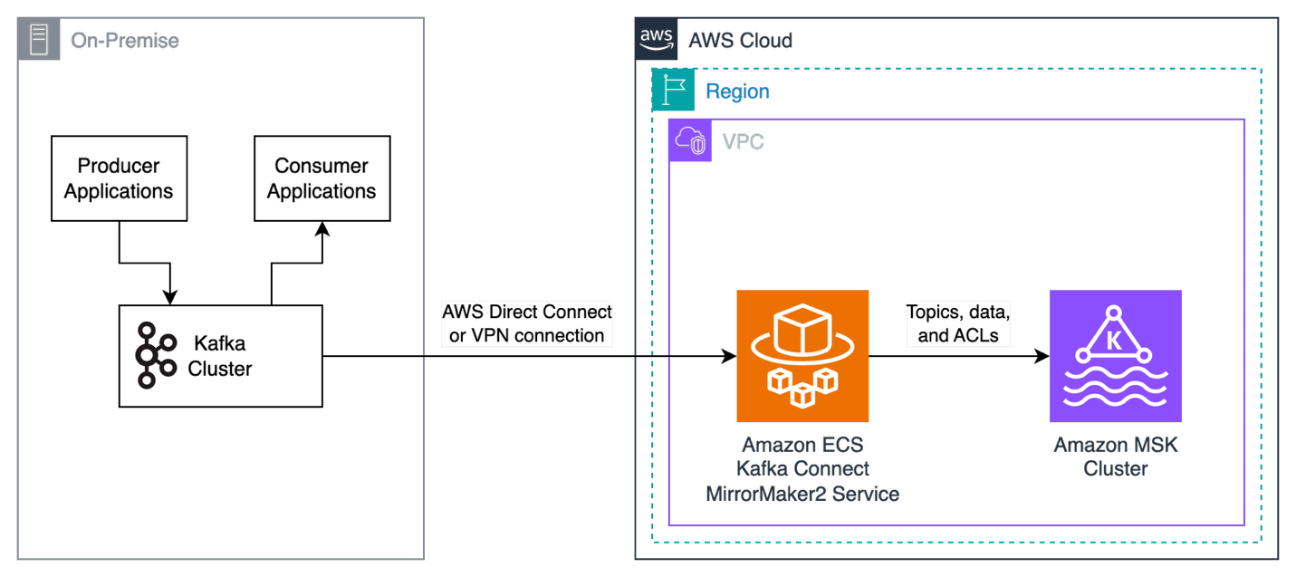
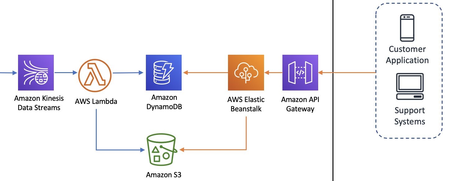
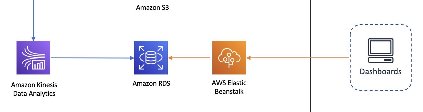
The following diagram shows the sequence of events in which the data is generated, collected, and finally stored in Amazon Redshift as the SUPER data type.

Manufacturers are embracing the cloud solutions with connected machines and factories to transform and use data to make data-driven decisions so they can optimize operations, increase productivity, and improve availability while reducing costs.

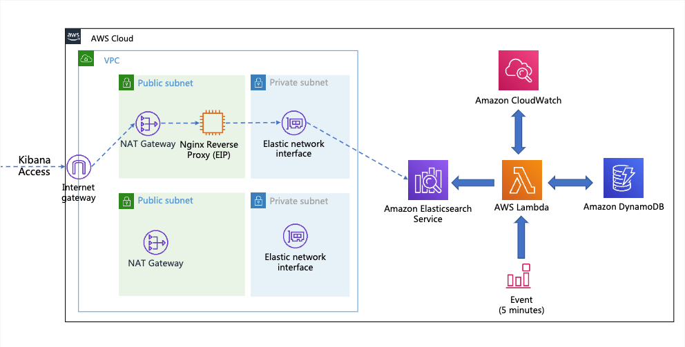
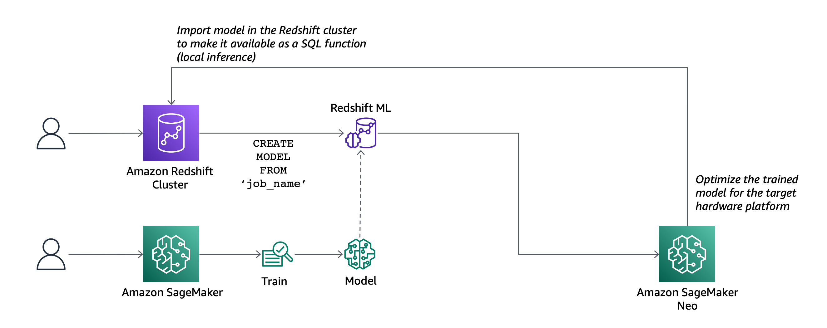
As an example, the following diagram depicts a common asset hierarchy of a fictional smart manufacturing company.

This data is typically semi-structured and hierarchical in nature. To find insights from this data using traditional methods and tools, you need to extract, preprocess, load, and transform it into the proper structured format to run typical analytical queries using a data warehouse. The time to insight is delayed because of the initial steps required for data cleansing and transformation typically performed using third-party tools or other AWS services.

Amazon Redshift SUPER handles these use cases by helping manufacturers extract, load, and query (without any transformation) a variety of data sources collected from edge computing and industrial IoT devices. Let’s use this sample dataset to drive our examples to explain the capabilities of Amazon Redshift SUPER.

The following is an example subscription dataset for assets (such as crowder, gauge, and pneumatic cylinder) in the workshop, which collects metrics on different properties (such as air pressure, machine state, finished parts count, and failures). Data on these metrics is generated continuously in a time series fashion and pushed to the AWS Cloud using the AWS IoT SiteWise connector. This specific example collects the Machine State property for an asset. The following sample data called subscriptions.json has scalar columns like topicId and qos, and a nested array called messages, which has metrics on the assets.

The following is another dataset called asset_metadata.json, which describes different assets and their properties, more like a dimension table. In this example, the asset_name is IAH10 Line 1, which is a processing plant line for a specific site.

Load data into SUPER columns

Now that we covered the basics behind Amazon Redshift SUPER and the industrial IoT use case, let’s look at different ways to load this dataset.

Copy the JSON document into multiple SUPER data columns

In this use case for handling semi-structured data, the user knows the incoming data’s top-level schema and structure, but some of the columns are semi-structured and nested in structures or arrays. You can choose to shred a JSON document into multiple columns that can be a combination of the SUPER data type and Amazon Redshift scalar types. The following code shows what the table DDL looks like if we translate the subscriptions.json semi-structured schema into a SUPER equivalent:

CREATE TABLE subscription_auto (
topicId INT
,topicFilter VARCHAR
,qos INT
,messages SUPER
);

To load data into this table, specify the auto option along with FORMAT JSON in the COPY command to split the JSON values across multiple columns. The COPY matches the JSON attributes with column names and allows nested values, such as JSON arrays and objects, to be ingested as SUPER values. Run the following command to ingest data into the subscription_auto table. Replace the AWS Identity and Access Management (IAM) role with your own credentials. The ignorecase option passed along with auto is required only if your JSON attribute names are in CamelCase. In our case, our columns topicId and topicFilter scalar columns are in CamelCase.

COPY subscription_auto FROM 's3://redshift-downloads/semistructured/super-blog/subscriptions/' 
IAM_ROLE '<< your IAM role >>' 
FORMAT JSON 'auto ignorecase';

A select * from subscription_auto command looks like the following code. The messages SUPER column holds the entire array in this case.

-- A sample output
SELECT * FROM subscription_auto;
[ RECORD 1 ]
topicid     | 1001
topicfilter | $aws/sitewise/asset-models/+/assets/+/properties/+
qos         | 0
messages    | [{"format":"json","topic":"$aws\/sitewise\/asset-models\/8926cf44-14ea-4cd8-a7c6-e61af641dbeb\/assets\/0aaf2aa2-0299-442a-b2ea-ecf3d62f2a2c\/properties\/3ff67d41-bf69-4d57-b461-6f1513e127a4","timestamp":1616381297183,"payload":{"type":"PropertyValueUpdate","payload":{"assetId":"0aaf2aa2-0299-442a-b2ea-ecf3d62f2a2c","propertyId":"3ff67d41-bf69-4d57-b461-6f1513e127a4","values":[{"timestamp":{"timeInSeconds":1616381289,"offsetInNanos":425000000},"quality":"GOOD","value":{"doubleValue":0}},{"timestamp":{"timeInSeconds":1616381292,"offsetInNanos":425000000},"quality":"FAIR","value":{"doubleValue":0}},{"timestamp":{"timeInSeconds":1616381286,"offsetInNanos":425000000},"quality":"GOOD","value":{"doubleValue":0}},{"timestamp":{"timeInSeconds":1616381293,"offsetInNanos":425000000},"quality":"GOOD","value":{"doubleValue":0}},{"timestamp":{"timeInSeconds":1616381287,"offsetInNanos":425000000},"quality":"GOOD","value":{"doubleValue":0}},{"timestamp":{"timeInSeconds":1616381290,"offsetInNanos":425000000},"quality":"GOOD","value":{"doubleValue":0}},{"timestamp":{"timeInSeconds":1616381290,"offsetInNanos":925000000},"quality":"GOOD","value":{"doubleValue":0}},{"timestamp":{"timeInSeconds":1616381294,"offsetInNanos":425000000},"quality":"FAIR","value":{"doubleValue":0}},{"timestamp":{"timeInSeconds":1616381285,"offsetInNanos":425000000},"quality":"GOOD","value":{"doubleValue":0}},{"timestamp":{"timeInSeconds":1616381288,"offsetInNanos":425000000},"quality":"GOOD","value":{"doubleValue":0}}]}}}]

Alternatively, you can specify jsonpaths to load the same data, as in the following code. The jsonpaths option is helpful if you want to load only selective columns from your JSON document. For more information, see COPY from JSON format.

COPY subscription_auto FROM 's3://redshift-downloads/semistructured/super-blog/subscriptions/' 
IAM_ROLE '<< your IAM role >>' 
FORMAT JSON 's3://redshift-downloads/semistructured/super-blog/jsonpaths/subscription_jsonpaths.json';

subscription_jsonpaths.json looks like the following:

{"jsonpaths": [
    "$.topicId",
    "$.topicFilter",
    "$.qos",
    "$.messages"
   ]
}

While we’re in the section about loading, let’s also create the asset_metadata table and load it with relevant data, which we need in our later examples. The asset_metadata table has more information about industry shop floor assets and their properties like asset_name, property_name, and model_id.

CREATE TABLE asset_metadata (
asset_id VARCHAR
,asset_name VARCHAR
,asset_model_id VARCHAR
,asset_property_id VARCHAR
,asset_property_name VARCHAR
,asset_property_data_type VARCHAR
,asset_property_unit VARCHAR
,asset_property_alias VARCHAR
);

COPY asset_metadata FROM 's3://redshift-downloads/semistructured/super-blog/asset_metadata/' 
IAM_ROLE '<< your IAM role >>' 
FORMAT JSON 'auto';

Copy the JSON document into a single SUPER column

You can also load a JSON document into a single SUPER data column. This is typical when the schema of the incoming JSON is unknown and evolving. SUPER’s schema-less ingestion comes to the forefront here, letting you load the data in a flexible fashion.

For this use case, assume that we don’t know the names of the columns in subscription.json and want to load it into Amazon Redshift. It’s as simple as the following code:

CREATE TABLE subscription_noshred (s super);

After the table is created, we can use the COPY command to ingest data from Amazon Simple Storage Service (Amazon S3) into the single SUPER column. The noshred is a required option to go along with FORMAT JSON, which tells the COPY parser not to shred the document but load it into a single column.

COPY subscription_noshred FROM 's3://redshift-downloads/semistructured/super-blog/subscriptions/' 
IAM_ROLE '<< your IAM role >>' 
FORMAT JSON 'noshred';

After the COPY has successfully ingested the JSON, the subscription_noshred table has a SUPER column s that contains the data of the entire JSON object. The ingested data maintains all the properties of the JSON nested structure but in a SUPER data type.

The following code shows how select star (*) into subscription_noshred looks; the entire JSON structure is in SUPER column s:

--A sample output
SELECT * FROM subscription_noshred;
[ RECORD 1 ]
s | {"topicId":1001,"topicFilter":"$aws\/sitewise\/asset-models\/+\/assets\/+\/properties\/+","qos":0,"messages":[{"format":"json","topic":"$aws\/sitewise\/asset-models\/8926cf44-14ea-4cd8-a7c6-e61af641dbeb\/assets\/0aaf2aa2-0299-442a-b2ea-ecf3d62f2a2c\/properties\/3ff67d41-bf69-4d57-b461-6f1513e127a4","timestamp":1616381297183,"payload":{"type":"PropertyValueUpdate","payload":{"assetId":"0aaf2aa2-0299-442a-b2ea-ecf3d62f2a2c","propertyId":"3ff67d41-bf69-4d57-b461-6f1513e127a4","values":[{"timestamp":{"timeInSeconds":1616381289,"offsetInNanos":425000000},"quality":"GOOD","value":{"doubleValue":0}},{"timestamp":{"timeInSeconds":1616381292,"offsetInNanos":425000000},"quality":"FAIR","value":{"doubleValue":0}},{"timestamp":{"timeInSeconds":1616381286,"offsetInNanos":425000000},"quality":"GOOD","value":{"doubleValue":0}},{"timestamp":{"timeInSeconds":1616381293,"offsetInNanos":425000000},"quality":"GOOD","value":{"doubleValue":0}},{"timestamp":{"timeInSeconds":1616381287,"offsetInNanos":425000000},"quality":"GOOD","value":{"doubleValue":0}},{"timestamp":{"timeInSeconds":1616381290,"offsetInNanos":425000000},"quality":"GOOD","value":{"doubleValue":0}},{"timestamp":{"timeInSeconds":1616381290,"offsetInNanos":925000000},"quality":"GOOD","value":{"doubleValue":0}},{"timestamp":{"timeInSeconds":1616381294,"offsetInNanos":425000000},"quality":"FAIR","value":{"doubleValue":0}},{"timestamp":{"timeInSeconds":1616381285,"offsetInNanos":425000000},"quality":"GOOD","value":{"doubleValue":0}},{"timestamp":{"timeInSeconds":1616381288,"offsetInNanos":425000000},"quality":"GOOD","value":{"doubleValue":0}}]}}}]}

Similar to the noshred option, we can also use jsonpaths to load complete documents. This can be useful in cases where we want to extract additional columns, such as distribution and sort keys, while still loading the complete document as a SUPER column. In the following example, we map our first column to the root JSON object, while also mapping a distribution key to the second column, and a sort key to the third column.

subscription_sorted_jsonpaths.json looks like the following:

{"jsonpaths": [
"$",
"$.topicId",
"$.topicFilter"
]
}

CREATE TABLE subscription_sorted (
s super
,topicId INT
,topicFilter VARCHAR
) DISTKEY(topicFilter) SORTKEY(topicId);

COPY subscription_sorted FROM 's3://redshift-downloads/semistructured/super-blog/subscriptions/' 
IAM_ROLE '<< your IAM role >>' 
FORMAT JSON 's3://redshift-downloads/semistructured/superblog/jsonpaths/subscription_sorted_jsonpaths.json';

Copy data from columnar formats like Parquet and ORC

If your semi-structured or nested data is already available in either Apache Parquet or Apache ORC formats, you can use the COPY command with the SERIALIZETOJSON option to ingest data into Amazon Redshift. The Amazon Redshift table structure should match the number of columns and the column data types of the Parquet or ORC files. Amazon Redshift can replace any Parquet or ORC column, including structure and array types, with SUPER data columns. The following are the COPY examples to load from Parquet and ORC format:

--Parquet 
COPY subscription_auto FROM 's3://redshift-downloads/semistructured/super-blog/subscriptions_parquet/' 
IAM_ROLE '<< your IAM role >>' FORMAT PARQUET SERIALIZETOJSON;

--ORC 
COPY subscription_auto FROM 's3://redshift-downloads/semistructured/super-blog/subscriptions_orc/' 
IAM_ROLE '<< your IAM role >>' FORMAT ORC SERIALIZETOJSON;

Apart from COPY, you can load the same data in columnar format in Amazon S3 using Amazon Redshift Spectrum and the INSERT command. The following example assumes the Redshift Spectrum external schema super_workshop and the external table subscription_parquet is already created and available in the database.

We need to set an important session-level configuration parameter for this to work: SET json_serialization_enable TO true. For more information, see Serializing complex nested JSON. This session-level parameter allows you to query top-level nested collection columns as serialized JSON.

/* -- Set the GUC for JSON serialization -- */ 
SET json_serialization_enable TO true;

INSERT INTO subscription_parquet 
SELECT topicId
,topicFilter
,qos
,JSON_PARSE(messages) FROM super_workshop.subscription_parquet;

As of this writing, we can’t use the SUPER column as such as a distribution or sort key, but if we need to use one of the attributes in a SUPER column as a distribution a sort key and keep the entire SUPER column intact as a separate column, we can use the following code as a workaround (apart from the jsonpaths example described earlier). For example, let’s assume the column format within the array messages needs to be used a distribution key for the Amazon Redshift table:

SET json_serialization_enable TO true;

DROP TABLEIF EXISTS subscription_messages;

CREATE TABLE subscription_messages (
m_format VARCHAR
,m_messages super
) distkey (m_format);

--'format' scalar column is extracted from 'messages' super column 
INSERT INTO subscription_messages 
SELECT element.format::VARCHAR
,supercol FROM (
SELECT JSON_PARSE(messages) AS supercol FROM super_workshop.subscription_parquet
) AS tbl,tbl.supercol element;

Apart from using the Amazon Redshift COPY command, we can also ingest JSON-formatted data into Amazon Redshift using the traditional SQL INSERT command:

--Insert example 
INSERT INTO subscription_auto VALUES (
0000
,'topicFiltervalue'
,0000
,JSON_PARSE('[{"format":"json"},{"topic": "sample topic"},[1,2,3]]')
); 

The JSON_PARSE() function parses the incoming data in proper JSON format and helps convert it into the SUPER data type. Without the JSON_PARSE() function, Amazon Redshift treats and ingests the value as a single string into SUPER instead of a JSON-formatted value.

Query SUPER columns

Amazon Redshift uses the PartiQL language to offer SQL-compatible access to relational, semi-structured, and nested data. PartiQL’s extensions to SQL are straightforward to understand, treat nested data as first-class citizens, and seamlessly integrate with SQL. The PartiQL syntax uses dot notation and array subscript for path navigation when accessing nested data.

The Amazon Redshift implementation of PartiQL supports dynamic typing for querying semi-structured data. This enables automatic filtering, joining, and aggregation on the combination of structured, semi-structured, and nested datasets. PartiQL allows the FROM clause items to iterate over arrays and use unnest operations.

The following sections focus on different query access patterns that involve navigating the SUPER data type with path and array navigation, unnest, or joins.

Navigation

We may want to find an array element by its index, or we may want to find the positions of certain elements in their arrays, such as the first element or the last element. We can reference a specific element simply by using the index of the element within square brackets (the index is 0-based) and within that element we can reference an object or struct by using the dot notation.

Let’s use our subscription_auto table to demonstrate the examples. We want to access the first element of the array, and within that we want to know the value of the attribute format:

SELECT messages[0].format FROM subscription_auto ;
--A sample output
 format
--------
 "json"
 "json"
 "json"
(3 rows)

Amazon Redshift can also use a table alias as a prefix to the notation. The following example is the same query as the previous example:

SELECT sub.messages[0].format FROM subscription_auto AS sub;
--A sample output
 format
--------
 "json"
 "json"
 "json"
(3 rows)

You can use the dot and bracket notations in all types of queries, such as filtering, join, and aggregation. You can use them in a query in which there are normally column references. The following example uses a SELECT statement that filters results:

SELECT COUNT(*) FROM subscription_auto WHERE messages[0].format IS NOT NULL;
-- A sample output
 count
-------
    11
(1 row)

Unnesting and flattening

To unnest or flatten an array, Amazon Redshift uses the PartiQL syntax to iterate over SUPER arrays by using the FROM clause of a query. We continue with the previous example in the following code, which iterates over the array attribute messages values:

SELECT c.*, o FROM subscription_auto c, c.messages AS o WHERE o.topic='sample topic';
-- A sample output
                             messages                 |        o
------------------------------------------------------+--------------------------
[{"format":"json"},{"topic":"sample topic"},[1,2,3]]  | {"topic":"sample topic"}
(1 row)

The preceding query has one extension over standard SQL: the c.messages AS o, where o is the alias for the SUPER array messages and serves to iterate over it. In standard SQL, the FROM clause x (AS) y means “for each tuple y in table x.” Similarly, the FROM clause x (AS) y, if x is a SUPER value, translates to “for each (SUPER) value y in (SUPER) array value x.” The projection list can also use the dot and bracket notation for regular navigation.

When unnesting an array, if we want to get the array subscripts (starting from 0) as well, we can specify AT some_index right after unnest. The following examples iterates over both the array values and array subscripts:

SELECT o, index FROM subscription_auto c, c.messages AS o AT index 
WHERE o.topic='sample topic';

-- A sample output 
       o                  | index
--------------------------+-------
{"topic":"sample topic"}  | 1
(1 row)

If we have an array of arrays, we can do multiple unnestings to iterate into the inner arrays. The following example shows how we do it. Note that unnesting non-array expressions (the objects inside c.messages) are ignored, only the arrays are unnested.

SELECT messages, array, inner_array_element FROM subscription_auto c, c.messages AS array, array AS inner_array_element WHERE array = json_parse('[1,2,3]');

-- A sample output 
    messages                                          | array   | inner_array_element
------------------------------------------------------+---------+---------------------
[{"format":"json"},{"topic":"sample topic"},[1,2,3]]  | [1,2,3] | 1
[{"format":"json"},{"topic":"sample topic"},[1,2,3]]  | [1,2,3] | 2
[{"format":"json"},{"topic":"sample topic"},[1,2,3]]  | [1,2,3] | 3
(3 rows)

Dynamic typing

With the schema-less nature of semi-structured data, the same attributes within the JSON might have values of different types. For example, asset_id from our example might have initially started with integers and then because of a business decision changed into alphanumeric (string) values before finally settling on array type. Amazon Redshift SUPER handles this situation by using dynamic typing. Schema-less SUPER data is processed without the need to statically declare the data types before using them in a query. Dynamic typing is most useful in joins and GROUP BY clauses. Although deep comparing of SUPER column is possible, we recommend restricting the joins and aggregations to use the leaf-level scalar attribute for optimal performance. The following example uses a SELECT statement that requires no explicit casting of the dot and bracket expressions to the usual Amazon Redshift types:

SELECT messages[0].format,
        messages[0].topic
FROM subscription_auto
WHERE messages[0].payload.payload."assetId" > 0;
 
--A sample output
 format | topic
--------+-------
"json"  | "sample topic" 
(1 rows)

When your JSON attribute names are in mixed case or CamelCase, the following session parameter is required to query the data. In the preceding query, assetId is in mixed case. For more information, see SUPER configurations.

SET enable_case_sensitive_identifier to TRUE;

The greater than (>) sign in this query evaluates to true when messages[0].payload.payload."assetId" is greater than 0. In all other cases, the equality sign evaluates to false, including the cases where the arguments of the equality are different types. The messages[0].payload.payload."assetId" attribute can potentially contain a string, integer, array, or structure, and Amazon Redshift only knows that it is a SUPER data type. This is where dynamic typing helps in processing the schemaless data by evaluating the types at runtime based on the query. For example, processing the first record of “assetId” may result in an integer, whereas the second record can be a string, and so on. When using an SQL operator or function with dot and bracket expressions that have dynamic types, Amazon Redshift produces results similar to using a standard SQL operator or function with the respective static types. In this example, when the dynamic type of the path expression is an integer, the comparison with the integer 0 is meaningful. Whenever the dynamic type of “assetId” is any other data type except being an integer, the equality returns false.

For queries with joins and aggregations, dynamic typing automatically matches values with different dynamic types without performing a long CASE WHEN analysis to find out what data types may appear. The following code is an example of an aggregation query in which we count the number of topics:

SELECT messages[0].format,
count(messages[0].topic)
FROM subscription_auto WHERE messages[0].payload.payload."assetId" > 'abc' GROUP BY 1;

-- a sample output
 format | count
--------+-------
"json"  |   2
(1 row)

For the next join query example, we unnest and flatten the messages array from subscription_auto and join with the asset_metadata table to get the asset_name and property_name based on the asset_id and property_id, which we use as join keys.

Joins on SUPER should preferably be on an extracted path and avoid deep compare of the entire nested field for performance. In the following examples, the join keys used are on extracted path keys and not on the whole array:

SELECT c.topicId
,c.qos
,a.asset_name
,o.payload.payload."assetId"
,a.asset_property_name
,o.payload.payload."propertyId"
FROM subscription_auto AS c
,c.messages AS o -- o is the alias for messages array
,asset_metadata AS a
WHERE o.payload.payload."assetId" = a.asset_id AND o.payload.payload."propertyId" = a.asset_property_id AND o.payload.type = 'PropertyValueUpdate';
 
--A sample output 
 topicid | qos |  asset_name  |                assetId                 | asset_property_name |               propertyId
---------+-----+--------------+----------------------------------------+---------------------+----------------------------------------
    1001 |   0 | IAH10 Line 1 | "0aaf2aa2-0299-442a-b2ea-ecf3d62f2a2c" | stop                | "3ff67d41-bf69-4d57-b461-6f1513e127a4"
(1 row)

The following code is another join query that is looking for a count on the quality of the metrics collected for a specific asset (in this case IAH10 Line) and it is property (Machine State) and categorizes it based on the quality:

SELECT v.quality::VARCHAR
,count(*)
FROM subscription_auto AS c
,c.messages AS o -- o is the alias for messages array
,o.payload.payload.VALUES AS v -- v is the alias for values array 
,asset_metadata AS a 
WHERE o."assetId" = a.asset_name 
AND o."propertyId" = a.asset_property_name 
AND a.asset_name = 'IAH10 Line 1' 
AND a.asset_property_name = 'Machine State' 
GROUP BY v.quality;

-- A sample output 
quality   | count
----------+-------
CRITICAL  | 152 
GOOD      | 2926 
FAIR      | 722

Summary

This post discussed the benefits of the new SUPER data type and use cases in which nested data types can help improve storage efficiency, performance, or simplify analysis. Amazon Redshift SUPER along with PartiQL enables you to write queries over relational and hierarchical data model with ease. The next post in this series will focus on how to speed up frequent queries on SUPER columns using materialized views. Try it out and share your experience!


About the Authors

Satish Sathiya is a Senior Product Engineer at Amazon Redshift. He is an avid big data enthusiast who collaborates with customers around the globe to achieve success and meet their data warehousing and data lake architecture needs.


Runyao Chen is a Software Development Engineer at Amazon Redshift. He is passionate about MPP databases and has worked on SQL language features such as querying semistructured data using SUPER. In his spare time, he enjoys reading and exploring new restaurants.


Cody Cunningham is a Software Development Engineer at Amazon Redshift. He works on Redshift’s data ingestion, implementing new features and performance improvements, and recently worked on the ingestion support for SUPER.

Design patterns for an enterprise data lake using AWS Lake Formation cross-account access

Post Syndicated from Satish Sarapuri original https://aws.amazon.com/blogs/big-data/design-patterns-for-an-enterprise-data-lake-using-aws-lake-formation-cross-account-access/

In this post, we briefly walk through the most common design patterns adapted by enterprises to build lake house solutions to support their business agility in a multi-tenant model using the AWS Lake Formation cross-account feature to enable a multi-account strategy for line of business (LOB) accounts to produce and consume data from your data lake.

A modern data platform enables a community-driven approach for customers across various industries, such as manufacturing, retail, insurance, healthcare, and many more, through a flexible, scalable solution to ingest, store, and analyze customer domain-specific data to generate the valuable insights they need to differentiate themselves. Building a data lake on Amazon Simple Storage Service (Amazon S3), together with AWS analytic services, sets you on a path to become a data-driven organization.

Overview of Lake House Architecture on AWS

You can deploy data lakes on AWS to ingest, process, transform, catalog, and consume analytic insights using the AWS suite of analytics services, including Amazon EMR, AWS Glue, Lake Formation, Amazon Athena, Amazon QuickSight, Amazon Redshift, Amazon Elasticsearch Service (Amazon ES), Amazon Relational Database Service (Amazon RDS), Amazon SageMaker, and Amazon S3. These services provide the foundational capabilities to realize your data vision, in support of your business outcomes. You can deploy a common data access and governance framework across your platform stack, which aligns perfectly with our own Lake House Architecture.

Large enterprise customers require a scalable data lake with a unified access enforcement mechanism to support their analytics workload. For this, you want to use a single set of single sign-on (SSO) and AWS Identity and Access Management (IAM) mappings to attest individual users, and define a single set of fine-grained access controls across various services. The AWS Lake House Architecture encompasses a single management framework; however, the current platform stack requires that you implement workarounds to meet your security policies without compromising on the ability to drive automation, data proliferation, or scale.

The following diagram illustrates the Lake House architecture.

Lake Formation serves as the central point of enforcement for entitlements, consumption, and governing user access. Furthermore, you may want to minimize data movements (copy) across LOBs and evolve on data mesh methodologies, which is becoming more and more prominent.

Most typical architectures consist of Amazon S3 for primary storage; AWS Glue and Amazon EMR for data validation, transformation, cataloging, and curation; and Athena, Amazon Redshift, QuickSight, and SageMaker for end users to get insight.

Introduction to Lake Formation

Lake Formation is a fully managed service that makes it easy to build, secure, and manage data lakes. Lake Formation simplifies and automates many of the complex manual steps that are usually required to create data lakes. These steps include collecting, cleansing, moving, and cataloging data, and securely making that data available for analytics and ML.

Lake Formation provides its own permissions model that augments the IAM permissions model. This centrally defined permissions model enables fine-grained access to data stored in data lakes through a simple grant or revoke mechanism, much like a relational database management system (RDBMS). Lake Formation permissions are enforced at the table and column level (row level in preview) across the full portfolio of AWS analytics and ML services, including Athena and Amazon Redshift.

With the new cross-account feature of Lake Formation, you can grant access to other AWS accounts to write and share data to or from the data lake to other LOB producers and consumers with fine-grained access. Data lake data (S3 buckets) and the AWS Glue Data Catalog are encrypted with AWS Key Management Service (AWS KMS) customer master keys (CMKs) for security purposes.

Common lake house design patterns using Lake Formation

A typical lake house infrastructure has three major components:

  • Data producer – Publishes the data into the data lake
  • Data consumer – Consumes that data out from the data lake and runs predictive and business intelligence (BI) insights
  • Data platform – Provides infrastructure and an environment to store data assets in the form of a layer cake such as landing, raw, and curated (conformance) data, and establishes security controls between producers and consumers

Although you can construct a data platform in multiple ways, the most common pattern is a single-account strategy, in which the data producer, data consumer, and data lake infrastructure are all in the same AWS account. There is no consensus if using a single account or multiple accounts most of the time is better, but because of the regulatory, security, performance trade-off, we have seen customers adapting to a multi-account strategy in which data producers and data consumers are in different accounts and the data lake is operated from a central, shared account.

This raised the concern of how to manage the data access controls across multiple accounts that are part of the data analytics platform to enable seamless ingestion for producers as well as improved business autonomy and agility for the needs of consumers.

With the general availability of the Lake Formation cross-account feature, the ability to manage data-driven access controls is simplified and offers an RDBMS style of managing data lake assets for producers and consumers.

You can drive your enterprise data platform management using Lake Formation as the central location of control for data access management by following various design patterns that balance your company’s regulatory needs and align with your LOB expectation. The following table summarizes different design patterns.

Design Type Lake Formation Glue Data Catalog Storage (Amazon S3) Compute
Centralized Centralized Centralized Centralized De-Centralized
De-Centralized De-Centralized Centralized De- Centralized De-Centralized

We explain each design pattern in more detail, with examples, in the following sections.\

Terminology

We use the following terms throughout this post when discussing data lake design patterns:

  • LOB – The line of business, such as inventory, marketing, or manufacturing
  • Enterprise data lake account (EDLA) – A centralized AWS account for data lake storage with a centralized AWS Glue Data Catalog and Lake Formation
  • Producer – The process or application producing data for its LOB
  • Consumer – The consumer of the LOB data via AWS services (such as Athena, AWS Glue, Amazon EMR, Amazon Redshift Spectrum, AWS Lambda, and QuickSight)

Centralized data lake design

In a centralized data lake design pattern, the EDLA is a central place to store all the data in S3 buckets along with a central (enterprise) Data Catalog and Lake Formation. The respective LOB producer and consumer accounts have all the required compute to write and read data in and from the central EDLA data, and required fine-grained access is performed using the Lake Formation cross-account feature. That’s why this architecture pattern (see the following diagram) is called a centralized data lake design pattern.

For this post, we use one LOB as an example, which has an AWS account as a producer account that generates data, which can be from on-premises applications or within an AWS environment. This account uses its compute (in this case, AWS Glue) to write data into its respective AWS Glue database. The database is created in the central EDLA where all S3 data is stored using the database link created with the Lake Formation cross-account feature. The same LOB consumer account consumes data from the central EDLA via Lake Formation to perform advanced analytics using services like AWS Glue, Amazon EMR, Redshift Spectrum, Athena, and QuickSight, using the consumer AWS account compute. The following section provides an example.

Create your database, tables and register S3 locations

In the EDLA, complete the following steps:

  1. Register the EDLA S3 bucket path in Lake Formation.
  2. Create a database called edla_lob_a, which points to the EDLA S3 bucket for LOB-A.

  3. Create a customer table in this edla_lob_a database , which points to the EDLA S3 bucket.

The LOB-A producer account can directly write or update data into tables, and create, update, or delete partitions using the LOB-A producer account compute via the Lake Formation cross-account feature.

You can trigger the table creation process from the LOB-A producer AWS account via Lambda cross-account access.

Grant Lake Formation cross-account access

Grant full access to the LOB-A producer account to write, update, and delete data into the EDLA S3 bucket via AWS Glue tables.

If your EDLA and producer accounts are part of same AWS organization, you should see the accounts on the list. If not, you need to enter the AWS account number manually as an external AWS account.

The following screenshot shows the granted permissions in the EDLA for the LOB-A producer account.


When you grant permissions to another account, Lake Formation creates resource shares in AWS Resource Access Manager (AWS RAM) to authorize all the required IAM layers between the accounts. To validate a share, sign in to the AWS RAM console as the EDLA and verify the resources are shared.

The first time you create a share, you see three resources:

  • The AWS Glue Data Catalog in the EDLA
  • The database containing the tables you shared
  • The table resource itself

You only need one share per resource, so multiple database shares only require a single Data Catalog share, and multiple table shares within the same database only require a single database share.

For the share to appear in the catalog of the receiving account (in our case the LOB-A account), the AWS RAM admin must accept the share by opening the share on the Shared With Me page and accepting it.

If both accounts are part of the same AWS organization and the organization admin has enabled automatic acceptance on the Settings page of the AWS Organizations console, then this step is unnecessary.

If your EDLA Data Catalog is encrypted with a KMS CMK, make sure to add your LOB-A producer account root user as the user for this key, so the LOB-A producer account can easily access the EDLA Data Catalog for read and write permissions with its local IAM KMS policy. Data encryption keys don’t need any additional permissions, because the LOB accounts use the Lake Formation role associated with the registration to access objects in Amazon S3.

When you sign in with the LOB-A producer account to the AWS RAM console, you should see the EDLA shared database details, as in the following screenshot.

Create a database resource link in the LOB-A producer account

Resource links are pointers to the original resource that allow the consuming account to reference the shared resource as if it were local to the account. As a pointer, resource links mean that any changes are instantly reflected in all accounts because they all point to the same resource. No sync is necessary for any of this and no latency occurs between an update and its reflection in any other accounts.

  1. Create a resource link to the shared Data Catalog database from the EDLA called shared_edla_lob_a.
  2. Grant full access to the AWS Glue role in the LOB-A producer account for this newly created shared database link from the EDLA so a producer AWS Glue job can create, update, and delete tables and partitions.

You need to perform two grants: one on the database shared link and one on the target to the AWS Glue job role. Granting on the link allows it to be visible to end-users. Data-level permissions are granted on the target itself.

  1. Create an AWS Glue job using this role to create and write data into the EDLA database and S3 bucket location.

The AWS Glue table and S3 data are in a centralized location for this architecture, using the Lake Formation cross-account feature.

This completes the configuration of the LOB-A producer account remotely writing data into the EDLA Data Catalog and S3 bucket. You can create and share the rest of the required tables for this LOB using the Lake Formation cross-account feature.

Because your LOB-A producer created an AWS Glue table and wrote data into the Amazon S3 location of your EDLA, the EDLA admin can access this data and share the LOB-A database and tables to the LOB-A consumer account for further analysis, aggregation, ML, dashboards, and end-user access.

Share the database to the LOB-A consumer account

In the EDLA, you can share the LOB-A AWS Glue database and tables (edla_lob_a, which contains tables created from the LOB-A producer account) to the LOB-A consumer account (in this case, the entire database is shared).

Next, go to the LOB-A consumer account to accept the resource share in AWS RAM.

Accepting the shared database in AWS RAM of the LOB-A consumer account

Sign in with the LOB-A consumer account to the AWS RAM console. You should see the EDLA shared database details.

Accept this resource share request so you can create a resource link in the LOB-A consumer account.

Create a database resource link in the LOB-A consumer account

Create a resource link to a shared Data Catalog database from the EDLA as consumer_edla_lob_a.

Now, grant full access to the AWS Glue role in the LOB-A consumer account for this newly created shared database link from the EDLA so the consumer account AWS Glue job can perform SELECT data queries from those tables. You need to perform two grants: one on the database shared link and one on the target to the AWS Glue job role.

A grant on the resource link allows a user to describe (or see) the resource link, which allows them to point engines such as Athena at it for queries. A grant on the target grants permissions to local users on the original resource, which allows them to interact with the metadata of the table and the data behind it. Permissions of DESCRIBE on the resource link and SELECT on the target are the minimum permissions necessary to query and interact with a table in most engines.

Create an AWS Glue job using this role to read tables from the consumer database that is shared from the EDLA and for which S3 data is also stored in the EDLA as a central data lake store. This data is accessed via AWS Glue tables with fine-grained access using the Lake Formation cross-account feature.

This completes the process of granting the LOB-A consumer account remote access to data for further analysis.

This data can be accessed via Athena in the LOB-A consumer account. LOB-A consumers can also access this data using QuickSight, Amazon EMR, and Redshift Spectrum for other use cases.


De-centralized data lake design

In the de-centralized design pattern, each LOB AWS account has local compute, an AWS Glue Data Catalog, and a Lake Formation along with its local S3 buckets for its LOB dataset and a central Data Catalog for all LOB-related databases and tables, which also has a central Lake Formation where all LOB-related S3 buckets are registered in EDLA.

EDLA manages all data access (read and write) permissions for AWS Glue databases or tables that are managed in EDLA. It grants the LOB producer account write, update, and delete permissions on the LOB database via the Lake Formation cross-account share. It also grants read permissions to the LOB consumer account. The respective LOB’s local data lake admins grant required access to their local IAM principals.

Refer to the earlier details on how to share database, tables, and table columns from EDLA to the producer and consumer accounts via Lake Formation cross-account sharing via AWS RAM and resource links.

Each LOB account (producer or consumer) also has its own local storage, which is registered in the local Lake Formation along with its local Data Catalog, which has a set of databases and tables, which are managed locally in that LOB account by its Lake Formation admins.

Clean up

To avoid incurring future charges, delete the resources that were created as part of this exercise.

Delete the S3 buckets in the following accounts:

  • Producer account
  • EDLA account
  • Consumer account (if any)

Delete the AWS Glue jobs in the following accounts:

  • Producer account
  • Consumer account (if any)

Lake Formation limitations

This solution has the following limitations:

  • The spark-submit action on Amazon EMR is not currently supported
  • AWS Glue Context does not yet support column-level fine-grained permissions granted via the Lake Formation

Conclusion

This post describes how you can design enterprise-level data lakes with a multi-account strategy and control fine-grained access to its data using the Lake Formation cross-account feature. This can help your organization build highly scalable, high-performance, and secure data lakes with easy maintenance of its related LOBs’ data in a single AWS account with all access logs and grant details.


About the Authors

Satish Sarapuri is a Data Architect, Data Lake at AWS. He helps enterprise-level customers build high-performance, highly available, cost-effective, resilient, and secure data lakes and analytics platform solutions, which includes streaming and batch ingestions into the data lake. In his spare time, he enjoys spending time with his family and playing tennis.


UmaMaheswari Elangovan is a Principal Data Lake Architect at AWS. She helps enterprise and startup customers adopt AWS data lake and analytic services, and increases awareness on building a data-driven community through scalable, distributed, and reliable data lake infrastructure to serve a wide range of data users, including but not limited to data scientists, data analysts, and business analysts. She also enjoys mentoring young girls and youth in technology by volunteering through nonprofit organizations such as High Tech Kids, Girls Who Code, and many more.


Zach Mitchell is a Sr. Big Data Architect. He works within the product team to enhance understanding between product engineers and their customers while guiding customers through their journey to develop data lakes and other data solutions on AWS analytics services.


Field Notes: Accelerating Data Science with RStudio and Shiny Server on AWS Fargate

Post Syndicated from Chayan Panda original https://aws.amazon.com/blogs/architecture/field-notes-accelerating-data-science-with-rstudio-and-shiny-server-on-aws-fargate/

Data scientists continuously look for ways to accelerate time to value for analytics projects.  RStudio Server is a popular Integrated Development Environment (IDE) for R, which is used to render analytics visualizations for faster decision making. These visualizations are traditionally hosted on legacy unix servers along with Shiny Server to support analytics. In this previous blog, we provided a solution architecture to run Data Science use cases for medium to large enterprises across industry verticals.

In this post, we describe and deliver the infrastructure code to run a secure, scalable and highly available RStudio and Shiny Server installation on AWS. We use these services: AWS Fargate, Amazon Elastic Container Service (Amazon ECS), Amazon Elastic File System (Amazon EFS), AWS DataSync, and Amazon Simple Storage Service (Amazon S3). We will then demonstrate a Data Science use case in RStudio and create an application on Shiny. The use case discussed involves pre-processing a dataset, and training a machine learning model in RStudio. The goal is to build a shiny application to surface breast cancer prediction insights against a set of parameters to users.

Overview of solution

We show how to deploy a Open Source RStudio Server and a Shiny Server in a serverless architecture from an automated deployment pipeline built with AWS Developer Tools. This is illustrated in the diagram that follows. The deployment adheres to best practices for following an AWS Multi-Account strategy using AWS Organizations.

Figure 1. RStudio/Shiny Open Source Deployment Pipeline on AWS Serverless Infrastructure

Figure 1. RStudio/Shiny Open Source Deployment Pipeline on AWS Serverless Infrastructure

Multi-Account Setup

In the preceding architecture, a central development account hosts the development resources. From this account, the deployment pipeline creates AWS services for RStudio and Shiny along with the integrated services into another AWS account. There can be multiple RStudio/Shiny accounts and instances to suit your requirements. You can also host multiple non-production instances of RStudio/Shiny in a single account.

Public URL Domain and Data Feed

The RStudio/Shiny deployment accounts obtain the networking information for the publicly resolvable domain from a central networking account. The data feed for the containers comes from a central data repository account. Users upload data to the S3 buckets in the central data account or configure an automated service like AWS Transfer Family to programmatically upload files. AWS DataSync transfers the uploaded files from Amazon S3 and stores the files on Amazon EFS mount points on the containers. Amazon EFS provides shared, persistent, and elastic storage for the containers.

Security Footprint

We recommend that you configure AWS Shield or AWS Shield Advanced for the networking account and enable Amazon GuardDuty in all accounts. You can also use AWS Config and AWS CloudTrail for monitoring and alerting on security events before deploying the infrastructure code. You should use an outbound filter such as AWS Network Firewall for network traffic destined for the internet. AWS Web Application Firewall (AWS WAF) protects the Amazon Elastic Load Balancers (Amazon ELB). You can restrict access to RStudio and Shiny from only allowed IP ranges using the automated pipeline.

High Availability

You deploy all AWS services in this architecture in one particular AWS Region. The AWS services used are managed services and configured for high availability. Should a service become unavailable, it automatically launches in the same Availability Zone (AZ) or in a different AZ within the same AWS Region. This means if Amazon ECS restarts the container in another AZ, following a failover, the files and data for the container will not be lost as these are stored on Amazon EFS.

Deployment

The infrastructure code provided in this blog creates all resources described in the preceding architecture. The following numbered items refer to Figure 1.

1. We used AWS Cloud Development Kit (AWS CDK) for Python to develop the infrastructure code and stored the code in an AWS CodeCommit repository.
2. AWS CodePipeline integrates the AWS CDK stacks for automated builds. The stacks are divided into four different stages and are organized by AWS service.
3. AWS CodePipeline fetches the container images from public Docker Hub and stores the images into Amazon Elastic Container Registry (Amazon ECR) repositories for cross-account access. The deployment pipeline accesses these images to create the Amazon ECS container on AWS Fargate in the deployment accounts.
4. The build script uses a key from AWS Key Management Service (AWS KMS) to create secrets. These include a RStudio front-end password, public key for bastion containers, and central data account access keys in AWS Secrets Manager. The deployment pipeline uses these secrets to configure the cross-account containers.
5. The central networking account Amazon Route 53 has the pre-configured base public domain. This is done outside the automated pipeline and the base domain info is passed on as a parameter to the deployment pipeline.
6. The central networking account delegates the base public domain to the RStudio deployment accounts via AWS Systems Manager (SSM) Parameter Store.
7. An AWS Lambda function retrieves the delegated Route 53 zone for configuring the RStudio and Shiny sub-domains.
8. AWS Certificate Manager configures encryption in transit by applying HTTPS certificates on the RStudio and Shiny sub-domains.
9. The pipeline configures an Amazon ECS cluster to control the RStudio, Shiny and Bastion containers and to scale up and down the number of containers as needed.
10. The pipeline creates RStudio container for the instance in a private subnet. RStudio container is not horizontally scalable for the Open Source version of RStudio.
– If you create only one container, the container will be configured for multiple front-end users. You need to specify the user names as email ids in cdk.json.
– Users receive their passwords and Rstudio/Shiny URLs via emails using Amazon Simple Email Service (SES).
– You can also create one RStudio container for each Data Scientist depending on your compute requirements by setting the cdk.json parameter individual_containers to true. You can also control the container memory/vCPU using cdk.json.
– Further details are provided in the readme. If your compute requirements exceed Fargate container compute limits, consider using EC2 launch type of Amazon ECS which offers a range of Amazon EC2 servers to fit your compute requirement. You can specify your installation type in cdk.json and choose either Fargate or EC2 launcg type for your RStudio containers.
11. To help you SSH to RStudio and Shiny containers for administration tasks, the pipeline creates a Bastion container in the public subnet. A Security Group restricts access to the bastion container and you can only access it from the IP range you provide in the cdk.json.
12. Shiny containers are horizontally scalable and the pipeline creates the Shiny containers in the private subnet using Fargate launch type of Amazon ECS. You can specify the number of containers you need for Shiny Server in cdk.json.
13. Application Load Balancers route traffic to the containers and perform health checks. The pipeline registers the RStudio and Shiny load balancers with the respective Amazon ECS services.
14. AWS WAF rules are built to provide additional security to RStudio and Shiny endpoints. You can specify approved IPs to restrict access to RStudio and Shiny from only allowed IPs.
15. Users upload files to be analysed to a central data lake account either with manual S3 upload or programmatically using AWS Transfer for SFTP.
16. AWS DataSync transfers files from Amazon S3 to cross-account Amazon EFS on an hourly interval schedule.
17. An AWS Lambda initiates DataSync transfer on demand outside of the hourly schedule for files that require urgent analysis. It is expected that bulk of the data transfer will happen on the hourly schedule and on-demand trigger will only be used when necessary.
18. Amazon EFS file systems provide shared, persistent and elastic storage for the containers. This is to facilitate deployment of Shiny Apps from RStudio containers using shared file system. The EFS file systems will live through container recycles.
19. You can create Amazon Athena tables on the central data account S3 buckets for direct interaction using JDBC from the RStudio container. Access keys for cross account operation are stored in the RStudio container R environment.

Note: It is recommended that you implement short term credential vending for this operation.

The source code for this deployment can be found in the aws-samples GitHub repository.

Prerequisites

To deploy the cdk stacks from the source code, you should have the following prerequisites:

1. Access to four AWS accounts (minimum three) for a basic multi-account deployment.
2. Permission to deploy all AWS services mentioned in the solution overview.
3. Review RStudio and Shiny Open Source Licensing: AGPL v3 (https://www.gnu.org/licenses/agpl-3.0-standalone.html)
4. Basic knowledge of R, RStudio Server, Shiny Server, Linux, AWS Developer Tools (AWS CDK in Python, AWS CodePipeline, AWS CodeCommit), AWS CLI and, the AWS services mentioned in the solution overview
5. Ensure you have a Docker hub login account, otherwise you might get an error while pulling the container images from Docker Hub with the pipeline – You have reached your pull rate limit. You may increase the limit by authenticating and upgrading: https://www.docker.com/increase-rate-limits.
6. Review the readmes delivered with the code and ensure you understand how the parameters in cdk.json control the deployment and how to prepare your environment to deploy the cdk stacks via the pipeline detailed below.

Installation

Create the AWS accounts to be used for deployment and ensure you have admin permissions access to each account. Typically, the following accounts are required:

Central Development account – this is the account where the AWS Secret Manager parameters, AWS CodeCommit repository, Amazon ECR repositories, and AWS CodePipeline will be created.
Central Network account – the Route53 base public domain will be hosted in this account
Rstudio instance account – You can use as many of these accounts as required, this account will deploy RStudio and Shiny containers for an instance (dev, test, uat, prod) along with a bastion container and associated  services as described in the solution architecture.
Central Data account – this is the account to be used for deploying the data lake resources – such as S3 bucket for selecting up ingested source files.

1. Install AWS CLI and create an AWS CLI profile for each account (pipeline, rstudio, network, datalake ) so that AWS CDK can be used.
2. Install AWS CDK in Python and bootstrap each account and allow the Central Development account to perform cross-account deployment to all the other accounts.

export CDK_NEW_BOOTSTRAP=1
npx cdk bootstrap --profile <AWS CLI profile of central development account> --cloudformation-execution-policies arn:aws:iam::aws:policy/AdministratorAccess aws://<Central Development Account>/<Region>

cdk bootstrap \
--profile <AWS CLI profile of rstudio deployment account> \
--trust <Central Development Account> \
--cloudformation-execution-policies arn:aws:iam::aws:policy/AdministratorAccess \
aws://<RStudio Deployment Account>/<Region>

cdk bootstrap \
--profile <AWS CLI profile of central network account> \
--trust <Central Development Account> \
--cloudformation-execution-policies arn:aws:iam::aws:policy/AdministratorAccess \
aws://<Central Network Account>/<Region>

cdk bootstrap \
--profile <AWS CLI profile of central data account> \
--trust <Central Development Account> \
--cloudformation-execution-policies arn:aws:iam::aws:policy/AdministratorAccess \
aws://<Central Data Account>/<Region>

3. Build the Docker container images in Amazon ECR in the central development account by running the image build pipeline as instructed in the readme.
a. Using the AWS console, create an AWS CodeCommit repository to hold the source code for building the images – for example, rstudio_docker_images.
b. Clone the GitHub repository and move into the image-build folder.
c. Using the CLI – Create a secret to store your DockerHub login details as follows:

aws secretsmanager create-secret --profile <AWS CLI profile of central development account> --name ImportedDockerId --secret-string '{"username":"<dockerhub username>", "password":"<dockerhub password>"}'

d. Create an AWS CodeCommit repository to hold the source code for building the images – e.g. rstudio_docker_images and pass the repository name to the name parameter in cdk.json for the image build pipeline
e. Pass the account numbers (comma separated) where rstudio instances will be deployed in the cdk.json paramter rstudio_account_ids
f. Synthesize the image build stack

cdk synth --profile <AWS CLi profile of central development account>

g. Commit the changes into the AWS CodeCommit repo you created using GitHub.
h. Deploy the pipeline stack for container image build.

cdk deploy --profile <AWS CLI profile of central development account>

i. Log into AWS console in the central development account and navigate to CodePipeline service. Monitor the pipeline (pipeline name is the name you provided in the name parameter in cdk.json) and confirm the docker images build successfully.

4. Move into the rstudio-fargate folder. Provide the comma separated accounts where rstudio/shiny will be deployed in the cdk.json against the parameter rstudio_account_ids.

5. Synthesize the stack Rstudio-Configuration-Stack in the Central Development account.

cdk synth Rstudio-Configuration-Stack --profile <AWS CLI profile of central development account> 

6. Deploy the Rstudio-Configuration-Stack. This stack should create a new CMK KMS Key to use for creating the secrets with AWS Secrets Maanger. The stack will output the AWS ARN for the KMS key. Note down the ARN. Set the parameter “encryption_key_arn” inside cdk.json to the above ARN.

cdk deploy Rstudio-Configuration-Stack --profile <AWS CLI profile of rstudio deployment account>

7. Run the script rstudio_config.sh after setting the required cdk.json parameters. Refer readme.

sh ./rstudio_config.sh <AWS CLI profile of the central development account> "arn:aws:kms:<region>:<AWS CLI profile of central development account>:key/<key hash>" <AWS CLI profile of central data account> <comma separated AWS CLI profiles of the rstudio deployment accounts>

8. Run the script check_ses_email.sh with comma separated profiles for rstudio deployment accounts. This will check whether all user emails have been registed with Amazon SES for all the rstudio deployment accounts in the region, before you can deploy rstudio/shiny.

sh ./check_ses_email.sh <comma separated AWS CLI profiles of the rstudio deployment accounts>

9. Before committing the code into the AWS CodeCommit repository, synthesize the pipeline stack against all the accounts involved in this deployment. This ensures all the necessary context values are populated into cdk.context.json file and to avoid the DUMMY values being mapped.

cdk synth --profile <AWS CLI profile of the central development account>
cdk synth --profile <AWS CLI profile of the central network account>
cdk synth --profile <AWS CLIrepeat for each profile of the RStudio deplyment account>

10. Deploy the Rstudio Fargate pipeline stack.

cdk deploy --profile <AWS CLI profile of the central development account> Rstudio-Piplenine-Stack

Data Science use case

Now the installation is completed. We can demonstrate a typical data science use case:

  1. Explore, and pre-process a dataset, and train a machine learning model in RStudio,
  2. Build a Shiny application that makes prediction against the trained model to surface insight to dashboard users.

This showcases how to publish a Shiny application from RStudio containers to Shiny containers via a common EFS filesystem.

First, we log on to the RStudio container with the URL from the deployment and clone the accompanying repository using the command line terminal. The ML example is in ml_example directory. We use the UCI Breast Cancer Wisconsin (Diagnostic) dataset from mlbench library. Refer to the ml_example/breast_cancer_modeling.r.

$ git clone https://github.com/aws-samples/aws-fargate-with-rstudio-open-source.git
Figure 2. Use the terminal to clone the repository in RStudio IDE.

Figure 2 – Use the terminal to clone the repository in RStudio IDE.

Let’s open the ml_example/breast_cancer_modeling.r script in the RStudio IDE. The script does the following:

  1. Install and import the required libraries, mainly caret, a popular machine learning library, and mlbench, a collection of ML datasets;
  2. Import the UCI breast cancer dataset, create an 80/20 split for training and testing (in shiny app) purposes;
  3. Perform preprocessing to impute the missing values (shown as NA) in the dataframe and standardize the numeric columns;
  4. Train a stochastic gradient boosting model with cross-validation with the area under the ROC curve (AUC) as the tuning metric;
  5. Save the testing split, preprocessing object and the trained model into the directory where shiny app script is located/breast-cancer-prediction.

You can execute the whole script with this command in the console.

> source('~/aws-fargate-with-rstudio-open-source/ml_example/breast_cancer_modeling.r')

We can then inspect the model evaluation in the model object gbmFit.

> gbmFit
Stochastic Gradient Boosting 

560 samples
  9 predictor
  2 classes: 'benign', 'malignant' 

No pre-processing
Resampling: Cross-Validated (10 fold, repeated 10 times) 
Summary of sample sizes: 504, 505, 503, 504, 504, 504, ... 
Resampling results across tuning parameters:

  interaction.depth  n.trees  ROC        Sens       Spec     
  1                   50      0.9916391  0.9716967  0.9304474
  1                  100      0.9917702  0.9700676  0.9330789
  1                  150      0.9911656  0.9689790  0.9305000
  2                   50      0.9922102  0.9708859  0.9351316
  2                  100      0.9917640  0.9681682  0.9346053
  2                  150      0.9910501  0.9662613  0.9361842
  3                   50      0.9922109  0.9689865  0.9381316
  3                  100      0.9919198  0.9684384  0.9360789
  3                  150      0.9912103  0.9673348  0.9345263

If the results are as expected, move on to developing a dashboard and publishing the model for business users to consume the machine learning insights.

In the repository, ml_example/breast-cancer-prediction/app.R has a Shiny application that displays a summary statistics and distribution of the testing data, and an interactive dashboard. This allows users to select data points on the chart and understand get the machine learning model inference as needed. Users can also modify the threshold to alter the specificity and sensitivity of the prediction. Thanks to the shared EFS filesystem across the RStudio and Shiny containers, we can publish the Shiny application with the following shell command to /srv/shiny-server.

$ cp ~/aws-fargate-with-rstudio-open-source/ml_example/breast-cancer-prediction/ \ /srv/shiny-server/ -rfv

That’s it. The Shiny application is now on the Shiny containers accessible from the Shiny URL, load balanced by Application Load Balancer. You can slide over the Probability Threshold to test how it changes the total count in the prediction, change the variables for the scatter plot and select data points to test the individual predictions.

shiny-dashboard-breast-cancer

Figure 3 – The Shiny Application

Cleaning up

Please follow the readme in the repository to delete the stacks created.

Conclusion

In this blog, we demonstrated how a serverless architecture can be deployed, walked through a data science use case in RStudio server and deployed an interactive dashboard in Shiny server. The solution creates a scalable, secure, and serverless data science environment for the R community that accelerates the data science process. The infrastructure and data science code is available in the github repository.

Field Notes provides hands-on technical guidance from AWS Solutions Architects, consultants, and technical account managers, based on their experiences in the field solving real-world business problems for customers.


Streaming Amazon DynamoDB data into a centralized data lake

Post Syndicated from Praveen Krishnamoorthy Ravikumar original https://aws.amazon.com/blogs/big-data/streaming-amazon-dynamodb-data-into-a-centralized-data-lake/

For organizations moving towards a serverless microservice approach, Amazon DynamoDB has become a preferred backend database due to its fully managed, multi-Region, multi-active durability with built-in security controls, backup and restore, and in-memory caching for internet-scale application. , which you can then use to derive near-real-time business insights. The data lake provides capabilities to business teams to plug in BI tools for analysis, and to data science teams to train models. .

This post demonstrates two common use cases of streaming a DynamoDB table into an Amazon Simple Storage Service (Amazon S3) bucket using Amazon Kinesis Data Streams, AWS Lambda, and Amazon Kinesis Data Firehose via Amazon Virtual Private Cloud (Amazon VPC) endpoints in the same AWS Region. We explore two use cases based on account configurations:

  • DynamoDB and Amazon S3 in same AWS account
  • DynamoDB and Amazon S3 in different AWS accounts

We use the following AWS services:

  • Kinesis Data Streams for DynamoDBKinesis Data Streams for DynamoDB captures item-level modifications in any DynamoDB table and replicates them to a Kinesis data stream of your choice. Your applications can access the data stream and view the item-level changes in near-real time. Streaming your DynamoDB data to a data stream enables you to continuously capture and store terabytes of data per hour. Kinesis Data Streams enables you to take advantage of longer data retention time, enhanced fan-out capability to more than two simultaneous consumer applications, and additional audit and security transparency. Kinesis Data Streams also gives you access to other Kinesis services such as Kinesis Data Firehose and Amazon Kinesis Data Analytics. This enables you to build applications to power real-time dashboards, generate alerts, implement dynamic pricing and advertising, and perform sophisticated data analytics, such as applying machine learning (ML) algorithms.
  • Lambda – Lambda lets you run code without provisioning or managing servers. It provides the capability to run code for virtually any type of application or backend service without managing servers or infrastructure. You can set up your code to automatically trigger from other AWS services or call it directly from any web or mobile app.
  • Kinesis Data Firehose – Kinesis Data Firehose helps to reliably load streaming data into data lakes, data stores, and analytics services. It can capture, transform, and deliver streaming data to Amazon S3 and other destinations. It’s a fully managed service that automatically scales to match the throughput of your data and requires no ongoing administration. It can also batch, compress, transform, and encrypt your data streams before loading, which minimizes the amount of storage used and increases security.

Security is the primary focus of our use cases, so the services used in both use server-side encryption at rest and VPC endpoints for securing the data in transit.

Use case 1: DynamoDB and Amazon S3 in same AWS account

In our first use case, our DynamoDB table and S3 bucket are in the same account. We have the following resources:

  • A Kinesis data stream is configured to use 10 shards, but you can change this as needed.
  • A DynamoDB table with Kinesis streaming enabled is a source to the Kinesis data stream, which is configured as a source to a Firehose delivery stream.
  • The Firehose delivery stream is configured to use a Lambda function for record transformation along with data delivery into an S3 bucket. The Firehose delivery stream is configured to batch records for 2 minutes or 1 MiB, whichever occurs first, before delivering the data to Amazon S3. The batch window is configurable for your use case. For more information, see Configure settings.
  • The Lambda function used for this solution transforms the DynamoDB item’s multi-level JSON structure to a single-level JSON structure. It’s configured to run in a private subnet of an Amazon VPC, with no internet access. You can extend the function to support more complex business transformations.

The following diagram illustrates the architecture of the solution.

The architecture uses the DynamoDB feature to capture item-level changes in DynamoDB tables using Kinesis Data Streams. This feature provides capabilities to securely stream incremental updates without any custom code or components.

Prerequisites

To implement this architecture, you need the following:

  • An AWS account
  • Admin access to deploy the needed resources

Deploy the solution

In this step, we create a new Amazon VPC along with the rest of the components.

We also create an S3 bucket with the following features:

You can extend the template to enable additional S3 bucket features as per your requirements.

For this post, we use an AWS CloudFormation template to deploy the resources. As part of best practices, consider organizing resources by lifecycle and ownership as needed.

We use an AWS Key Management Service (AWS KMS) key for server-side encryption to encrypt the data in Kinesis Data Streams, Kinesis Data Firehose, Amazon S3, and DynamoDB.

The Amazon CloudWatch log group data is always encrypted in CloudWatch Logs. If required, you can extend this stack to encrypt log groups using KMS CMKs.

  1. Click on Launch Stack button below to create a CloudFormation :
  2. On the CloudFormation console, accept default values for the parameters.
  3. Select I acknowledge that AWS CloudFormation might create IAM resources with custom names.
  4. Choose Create stack.

After stack creation is complete, note the value of the BucketName output variable from the stack’s Outputs tab. This is the S3 bucket name that is created as part of the stack. We use this value later to test the solution.

Test the solution

To test the solution, we insert a new item and then update the item in the DynamoDB table using AWS CloudShell and the AWS Command Line Interface (AWS CLI). We will also use the AWS Management Console to monitor and verify the solution.

  1. On the CloudShell console, verify that you’re in the same Region as the DynamoDB table (the default is us-east-1).
  2. Enter the following AWS CLI command to insert an item:
    aws dynamodb put-item \ 
    --table-name blog-srsa-ddb-table \ 
    --item '{ "id": {"S": "864732"}, "name": {"S": "Adam"} , "Designation": {"S": "Architect"} }' \ 
    --return-consumed-capacity TOTAL

  3. Enter the following command to update the item: We are updating the Designation from “Architect” to ” Senior Architect
    aws dynamodb put-item \ 
    --table-name blog-srsa-ddb-table \ 
    --item '{ "id": {"S": "864732"}, "name": {"S": "Adam"} , "Designation": {"S": "Senior Architect"} }' \ 
    --return-consumed-capacity TOTAL

All item-level modifications from the DynamoDB table are sent to a Kinesis data stream (blog-srsa-ddb-table-data-stream), which delivers the data to a Firehose delivery stream (blog-srsa-ddb-table-delivery-stream).

You can monitor the processing of updated records in the Firehose delivery stream on the Monitoring tab of the delivery stream.

You can verify the delivery of the updates to the data lake by checking the objects in the S3 bucket (BucketName value from the stack Outputs tab).

The Firehose delivery stream is configured to write records to Amazon S3 using a custom prefix which is based on the date the records are delivered to the delivery stream. This partitions the delivered records by date which helps improve query performance by limiting the amount of data that query engines need to scan in order to return the results for a specific query. For more information, see Custom Prefixes for Amazon S3 Objects.

The file is in JSON format. You can verify the data in the following ways:

Use case 2: DynamoDB and Amazon S3 in different AWS accounts

The solution for this use case uses two CloudFormation stacks: the producer stack (deployed in Account A) and the consumer stack (deployed in Account B).

The producer stack (Account A) deploys the following:

  • A Kinesis data stream is configured to use 10 shards, but you can change this as needed.
  • A DynamoDB table with Kinesis streaming is enabled as a source to the Kinesis data stream, and the data stream is configured as a source to a Firehose delivery stream.
  • The Firehose delivery stream is configured to use a Lambda function for record transformation along with data delivery into an S3 bucket in Account B. The delivery stream is configured to batch records for 2 minutes or 1 MiB, whichever occurs first, before delivering the data to Amazon S3. The batch window is configurable for your use case.
  • The Lambda function is configured to run in a private subnet of an Amazon VPC, with no internet access. For this solution, the function transforms the multi-level JSON structure to a single-level JSON structure. You can extend the function to support more complex business transformations.

The consumer stack (Account B) deploys an S3 bucket configured to receive the data from the Firehose delivery stream in Account A.

The following diagram illustrates the architecture of the solution.

The architecture uses the DynamoDB feature to capture item-level changes in DynamoDB tables using Kinesis Data Streams. This feature provides capabilities to securely stream incremental updates without any custom code or components. 

Prerequisites

For this use case, you need the following:

  • Two AWS accounts (for the producer and consumer)
    • If you already deployed the architecture for the first use case and want to use the same account, delete the stack from the previous use case before proceeding with this section
  • Admin access to deploy needed resources

Deploy the components in Account B (consumer)

This step creates an S3 bucket with the following features:

  • Encryption at rest using CMKs
  • Block Public Access
  • Bucket versioning

You can extend the template to enable additional S3 bucket features as needed.

We deploy the resources with a CloudFormation template. As part of best practices, consider organizing resources by lifecycle and ownership as needed.

We use the KMS key for server-side encryption to encrypt the data in Amazon S3.

The CloudWatch log group data is always encrypted in CloudWatch Logs. If required, you can extend the stack to encrypt log group data using KMS CMKs.

  1. Choose Launch Stack to create a CloudFormation stack in your account:
  2. For DDBProducerAccountID, enter Account A’s account ID.
  3. For KMSKeyAlias, the KMS key used for server-side encryption to encrypt the data in Amazon S3 is populated by default.
  4. Choose Create stack.

After stack creation is complete, note the value of the BucketName output variable. We use this value later to test the solution.

Deploy the components in Account A (producer)

In this step, we sign in to the AWS Management Console with Account A to deploy the producer stack. We use the KMS key for server-side encryption to encrypt the data in Kinesis Data Streams, Kinesis Data Firehose, Amazon S3, and DynamoDB. As with other stacks, the CloudWatch log group data is always encrypted in CloudWatch Logs, but you can extend the stack to encrypt log group data using KMS CMKs.

  1. Choose Launch Stack to create a CloudFormation stack in your account:
  2. For ConsumerAccountID, enter the ID of Account B.
  3. For CrossAccountDatalakeBucket, enter the bucket name for Account B, which you created in the previous step.
  4. For ArtifactBucket, the S3 bucket containing the artifacts required for deployment is populated by default.
  5. For KMSKeyAlias, the KMS key used for server-side encryption to encrypt the data in Amazon S3 is populated by default.
  6. For BlogTransformationLambdaFile, the Amazon S3 key for the Lambda function code to perform Amazon Firehose Data transformation is populated by default.
  7. Select I acknowledge that AWS CloudFormation might create IAM resources with custom names.
  8. Choose Create stack.

Test the solution

To test the solution, we sign in as Account A, insert a new item in the DynamoDB table, and then update that item. Make sure you’re in the same Region as your table.

  1. On the CloudShell console, enter the following AWS CLI command to insert an item:
    aws dynamodb put-item \ 
    --table-name blog-srca-ddb-table \ 
    --item '{ "id": {"S": "864732"}, "name": {"S": "Chris"} , "Designation": {"S": "Senior Consultant"} }' \ 
    --return-consumed-capacity TOTAL

  2. Update the existing item with the following code:
    aws dynamodb put-item \ 
    --table-name blog-srca-ddb-table \ 
    --item '{ "id": {"S": "864732"}, "name": {"S": "Chris"} , "Designation": {"S": "Principal Consultant"} }' \ 
    --return-consumed-capacity TOTAL

  3. Sign out of Account A and sign in as Account B to verify the delivery of records into the data lake.

All item-level modifications from an DynamoDB table are sent to a Kinesis data stream (blog-srca-ddb-table-data-stream), which delivers the data to a Firehose delivery stream (blog-srca-ddb-table-delivery-stream) in Account A.

You can monitor the processing of the updated records on the Monitoring tab of the Firehose delivery stream.

You can verify the delivery of updates to the data lake by checking the objects in the S3 bucket that you created in Account B.

The Firehose delivery stream is configured similarly to the previous use case.

You can verify the data (in JSON format) in the same ways:

  • Download the files
  • Run an AWS Glue crawler to create a table to query in Athena
  • Query the data using Amazon S3 Select

Clean up

To avoid incurring future charges, clean up all the AWS resources that you created using AWS CloudFormation. You can delete these resources on the console or via the AWS CLI. For this post, we walk through the steps using the console.

Clean up resources from use case 1

To clean up the DynamoDB and Amazon S3 resources in the same account, complete the following steps:

  1. On the Amazon S3 console, empty the S3 bucket and remove any previous versions of S3 objects.
  2. On the AWS CloudFormation console, delete the stack bdb1040-ddb-lake-single-account-stack.

You must delete the Amazon S3 resources before deleting the stack, or the deletion fails.

Clean up resources from use case 2

To clean up the DynamoDB and Amazon S3 resources in different accounts, complete the following steps:

  1. Sign in to Account A.
  2. On the AWS CloudFormation console, delete the stack bdb1040-ddb-lake-multi-account-stack.
  3. Sign in to Account B.
  4. On the Amazon S3 console, empty the S3 bucket and remove any pervious versions of S3 objects.
  5. On the AWS CloudFormation console, delete the stack bdb1040-ddb-lake-multi-account-stack.

Extend the solution

You can extend this solution to stream DynamoDB table data into cross-Region S3 buckets by setting up cross-Region replication (using the Amazon secured private channel) on the bucket where Kinesis Data Firehose delivers the data.

You can also perform a point-in-time initial load of the DynamoDB table into the data lake before setting up DynamoDB Kinesis streams. DynamoDB provides a no-coding required feature to achieve this. For more information, see Export Amazon DynamoDB Table Data to Your Data Lake in Amazon S3, No Code Writing Required.

To extend the usability scope of DynamoDB data in S3 buckets, you can crawl the location to create AWS Glue Data Catalog database tables. Registering the locations with AWS Lake Formation helps simplify permission management and allows you to implement fine-grained access control. You can also use Athena, Amazon Redshift, Amazon SageMaker, and Amazon QuickSight for data analysis, ML, and reporting services.

Conclusion

In this post, we demonstrated two solutions for streaming DynamoDB table data into Amazon S3 to build a data lake using a secured Amazon private channel.

The CloudFormation template gives you an easy way to set up the process, which you can be further modify to meet your specific use case needs.

Please let us know if you have comments about this post!


About the Authors

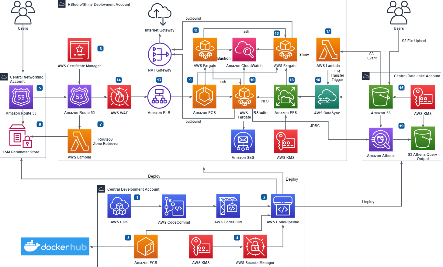
Praveen Krishnamoorthy Ravikumar is a Data Architect with AWS Professional Services Intelligence Practice. He helps customers implement big data and analytics platform and solutions.


Abhishek Gupta is a Data and ML Engineer with AWS Professional Services Practice.


Ashok Yoganand Sridharan is a Big Data Consultant with AWS Professional Services Intelligence Practice. He helps customers implement big data and analytics platform and solutions


Amazon MSK Replicator and MirrorMaker2: Choosing the right replication strategy for Apache Kafka disaster recovery and migrations

Post Syndicated from Anusha Dharmalingam original https://aws.amazon.com/blogs/big-data/amazon-msk-replicator-and-mirrormaker2-choosing-the-right-replication-strategy-for-apache-kafka-disaster-recovery-and-migrations/

Customers need to replicate their Apache Kafka for a variety of reasons, such as compliance requirements, cluster migrations, and disaster recovery (DR) implementations. However, the right replication strategy can vary depending on the application context. In this post, we walk through the different considerations for using Amazon MSK Replicator over Apache Kafka’s MirrorMaker 2, and help you choose the right replication solution for your use case. We also discuss how to make applications using Amazon Managed Streaming for Apache Kafka (Amazon MSK) resilient to disasters using a multi-Region Kafka architecture using MSK Replicator.

Challenges with choosing DR strategies

Customers create business continuity plans and DR strategies to maximize resiliency for their applications, because downtime or data loss can result in losing revenue or halting operations. DR planning helps the business continue running in the event of a disaster impacting a subset of their application architecture. For customers using Kafka as a core streaming and messaging service in their applications, planning for DR for their Kafka infrastructure is an essential part of meeting goals for their application Recovery Time Objective (RTO) and Recovery Point Objective (RPO).

Amazon MSK is a fully managed service that makes it straightforward to build and run Kafka to process streaming data. Amazon MSK provides high availability by offering multi-AZ configurations to distribute brokers across multiple Availability Zones within an AWS Region. A single MSK cluster deployment provides message durability through intra-cluster data replication. Data replication with a replication factor of 3 and min-ISR value of 2 along with the producer setting acks=all provides the strongest availability guarantees, because it makes sure other brokers in the cluster acknowledge receiving the data before the leader broker responds to the producer. This design provides robust protection against single broker failure as well as single-AZ failure.

For enhanced resilience within a single Region, Amazon MSK also offers Express brokers, which significantly improve Kafka cluster reliability, throughput, recovery times. Express brokers include pay-as-you-go storage, automatic best-practice reliability configurations, no maintenance windows, and faster broker scaling and recovery times. This architecture reduces recovery time, minimizes the chance of errors with misconfigurations, and increases throughput, making your Kafka clusters more resilient across Availability Zones.

However, if an unlikely issue is impacting your applications or infrastructure across more than one Availability Zone, the architecture outlined in this post can help you prepare, respond, and recover from it.

For companies that can withstand a longer RTO but require a lower RPO on Amazon MSK, backing up data to Amazon Simple Storage Service (Amazon S3) is sufficient as a DR plan. This approach requires you to think through how to handle restarting the application after a DR failover. In this approach, you build a system to recover the data from Amazon S3 to Kafka topics (as described in Back up and restore Kafka topic data using Amazon MSK Connect). Depending on the volume of data being restored, it might take a long time to recover in this scenario. Additionally, you must consider how to handle consumer group offsets, and whether to allow applications to consume from the latest offset in the restored Kafka topics. Due to the high RTO, as well as the complexity and challenges associated with this approach, most streaming use cases rely on the availability of the MSK cluster itself for their business continuity plan. In these cases, setting up MSK clusters in multiple Regions and configuring data replication between clusters provides the required business resilience and continuity.

Choosing the right replication solution: MSK Replicator vs MirrorMaker 2

AWS recommends two primary solutions for cross-Region Kafka replication: MSK Replicator and MirrorMaker 2. Understanding when to use each solution is crucial for designing an effective DR strategy.

MSK Replicator: For most MSK cluster replications in the same account

MSK Replicator is a fully managed, serverless Kafka replication service that makes it straightforward to reliably replicate data across MSK clusters in different Regions or within the same Region. MSK Replicator is the recommended solution for application scenarios replicating data within the same AWS account. MSK Replicator has the following benefits:

  • Replication between MSK clusters – It supports replicating between MSK clusters in the same AWS account (including active-active or active-passive DR architectures for Amazon MSK)
  • No infrastructure management – It’s fully serverless with automatic scaling and straightforward setup through the AWS Management Console, AWS Command Line Interface (AWS CLI), or APIs
  • Built-in monitoring – It’s integrated with Amazon CloudWatch metrics and logging
  • Built-in high availability – As a managed service, it offers built-in fault tolerance across Availability Zones

MirrorMaker 2: For migrations and complex and hybrid scenarios

MirrorMaker 2 (MM2) remains the preferred solution for specific use cases that require more flexibility or involve non-Amazon MSK environments. MM2 is a utility bundled as part of Kafka that helps replicate data between Kafka clusters using the Kafka Connect framework.

We recommend MirrorMaker 2 for the following use cases:

  • Cross-account replication – Replicating data between MSK clusters in different AWS accounts
  • Migrations to Amazon MSK – Migrating from existing Kafka clusters on premises, in other clouds, or on self-managed Amazon Elastic Compute Cloud (Amazon EC2) deployments
  • Cross-cloud or hybrid cloud scenarios – Replicating between Kafka running on-premises or on different cloud providers and Amazon MSK for disaster recovery or data analytics use cases
  • Using mTLS or SASL/SCRAM authentication – When you need mutual TLS certificate-based or SASL/SCRAM authentication and can’t enable AWS Identity and Access Management (IAM) authentication in your MSK cluster (for replication from one MSK cluster to another in these scenarios, you can still use MSK Replicator by enabling IAM authentication in addition to existing authentication methods)
  • Custom replication policies – Advanced topic naming or transformation requirements

In the following sections, we discuss the architecture and deployment approaches for use cases where MSK Replicator and MirrorMaker 2 are the appropriate choices.

MSK Replicator solution overview

The following diagram illustrates the architecture for using MSK Replicator.

We create two MSK clusters – one in the primary Region, the other in the secondary Region as a standby cluster for disaster recovery. We deploy MSK Replicator in the secondary region to replicate topics, ACLs, data, and consumer group offsets from the primary cluster. In this solution, we showcase a single-direction replication for active-passive disaster recovery. This solution can also be extended for active-active disaster recovery scenarios. Our Kafka clients connect to the primary cluster and can be configured to connect to the secondary cluster in the event of a disaster recovery failover.

For details on implementation steps, refer to Introducing Amazon MSK Replicator – Fully Managed Replication across MSK Clusters in Same or Different AWS Regions. For details on disaster recovery scenarios, refer to Use replication to increase the resiliency of a Kafka streaming application across Regions. These resources provide the following benefits:

  • Full deployment steps – Step by step deployment process for MSK Replicator between regions
  • Comprehensive examples – Multiple deployment scenarios and configurations
  • Failover process – Key steps in executing a disaster recovery failover when using MSK Replicator

MirrorMaker2 solution overview

The following diagram illustrates the architecture for using MirrorMaker 2.

We create an MSK cluster in the primary Region, with the existing Kafka cluster on premises. This Kafka cluster is analogous to Kafka clusters running in other clouds, or in self-managed Kafka clusters on Amazon EC2. In this solution, we showcase a single-direction replication for cluster migration scenarios. Our Kafka clients interact with the on-premises Kafka cluster and can be migrated to run on AWS to interact with the MSK cluster.

Rather than manually configuring each component, we recommend using the automated deployment resources available in the following GitHub repository. For a step-by-step walkthrough of deploying MirrorMaker 2 on Amazon ECS with Fargate using auto scaling, refer to Amazon MSK Migration Workshop: Modernizing with Express Brokers. These resources provide the following benefits:

  • Infrastructure as code – Terraform for MSK clusters and supporting infrastructure
  • Containerized Kafka Connect – Docker images optimized for AWS
  • Amazon ECS with AWS Fargate deployment – Scalable, serverless container deployment using Amazon Elastic Container Service (Amazon ECS) with AWS Fargate
  • Auto scaling configuration – Automatic scaling based on workload demands
  • Comprehensive examples – Multiple deployment scenarios and configurations
  • Migration process – Key steps in executing a Kafka migration using MM2

Conclusion

Choosing the right replication solution depends on your specific requirements. We recommend using MSK Replicator when replicating from one MSK cluster to another and you want a fully managed solution for disaster recovery. MirrorMaker 2 is recommended for migrations to Amazon MSK, hybrid environments, or when you need complex custom replication policies.

For MSK Replicator deployments, refer to Introducing Amazon MSK Replicator – Fully Managed Replication across MSK Clusters in Same or Different AWS Regions and Use replication to increase the resiliency of a Kafka streaming application across Regions.

For MirrorMaker 2 deployments, refer to the GitHub repository and Amazon MSK Migration Workshop to implement production-ready solutions with automated deployment, monitoring, and scaling capabilities.

These approaches provide a customizable set of options for data redundancy and business continuity capabilities needed to meet regulatory compliance and disaster recovery requirements, while minimizing operational overhead through automation and best practices.


About the Author

Mazrim Mehrtens

Mazrim Mehrtens

Mazrim is a Sr. Specialist Solutions Architect for messaging and streaming workloads. Mazrim works with customers to build and support systems that process and analyze terabytes of streaming data in real time, run enterprise Machine Learning pipelines, and create systems to share data across teams seamlessly with varying data toolsets and software stacks.

Preprocess logs for anomaly detection in Amazon ES

Post Syndicated from Kapil Pendse original https://aws.amazon.com/blogs/big-data/preprocess-logs-for-anomaly-detection-in-amazon-es/

Amazon Elasticsearch Service (Amazon ES) supports real-time anomaly detection, which uses machine learning (ML) to proactively detect anomalies in real-time streaming data. When used to analyze application logs, it can detect anomalies such as unusually high error rates or sudden changes in the number of requests. For example, a sudden increase in the number of food delivery orders from a particular area could be due to weather changes or due to a technical glitch experienced by users from that area. The detection of such an anomaly can facilitate quick investigation and remediation of the situation.

The anomaly detection feature of Amazon ES uses the Random Cut Forest algorithm. This is an unsupervised algorithm that constructs decision trees from numeric input data points in order to detect outliers in the data. These outliers are regarded as anomalies. To detect anomalies in logs, we have to convert the text-based log files into numeric values so that they can be interpreted by this algorithm. In ML terminology, such conversion is commonly referred to as data preprocessing. There are several methods of data preprocessing. In this post, I explain some of these methods that are appropriate for logs.

To implement the methods described in this post, you need a log aggregation pipeline that ingests log files into an Amazon ES domain. For information about ingesting Apache web logs, see Send Apache Web Logs to Amazon Elasticsearch Service with Kinesis Firehose. For a similar method for ingesting and analyzing Amazon Simple Storage Service (Amazon S3) server access logs, see Analyzing Amazon S3 server access logs using Amazon ES.

Now, let’s discuss some data preprocessing methods that we can use when dealing with complex structures within log files.

Log lines to JSON documents

Although they’re text files, usually log files have some structure to the log messages, with one log entry per line. As shown in the following image, a single line in a log file can be parsed and stored in an Amazon ES index as a document with multiple fields. This image is an example of how an entry in an Amazon S3 access log can be converted into a JSON document.

Although you can ingest JSON documents such as the preceding image as is into Amazon ES, some of the text fields require further preprocessing before you can use them for anomaly detection.

Text fields with nominal values

Let’s assume your application receives mostly GET requests and a much smaller number of POST requests. According to an OWASP security recommendation, it’s also advisable to disable TRACE and TRACK request methods because these can be misused for cross-site tracing. If you want to detect when unusual HTTP requests appear in your server logs, or when there is a sudden spike in the number of HTTP requests with methods that are normally a minority, you could do so by using the request_uri or operation fields in the preceding JSON document. These fields contain the HTTP request method, but you have to extract that and convert that into a numeric format that can be used for anomaly detection.

These are fields that have only a handful of different values, and those values don’t have any particular sequential order. If we simply convert HTTP methods to an ordered list of numbers, like GET = 1, POST = 2, and so on, we might confuse the anomaly detection algorithm into thinking that POST is somehow greater than GET, or that GET + GET equals POST. A better way to preprocess such fields is one-hot encoding. The idea is to convert the single text field into multiple binary fields, one for every possible value of the original text field. In our example, the result of this one-hot encoding is a set of nine binary fields. If the value of the field in the original log is HEAD, only the HEAD field in the preprocessed data has value 1, and all other fields are zero. The following table shows some examples.

Original Log Message Preprocessed into multiple one-hot encoded fields

HTTP Request Method

GET HEAD POST PUT DELETE CONNECT OPTIONS TRACE PATCH
GET 1 0 0 0 0 0 0 0 0
POST 0 0 1 0 0 0 0 0 0
OPTIONS 0 0 0 0 0 0 1 0 0

These generated fields data can be then processed by the Amazon ES anomaly detection feature to detect anomalies when there is a change in the pattern of HTTP requests received by your application, for example an unusually high number of DELETE requests.

Text fields with a large number of nominal values

Many log files contain HTTP response codes, error codes, or some other type of numeric codes. These codes don’t have any particular order, but the number of possible values is quite large. In such cases, one-hot encoding alone isn’t suitable because it can cause an explosion in the number of fields in the preprocessed data.

Take for example the HTTP response codes. The values are unordered, meaning that there is no particular reason for 200 being OK and 400 being Bad Request. 200 + 200 != 400 as far as HTTP response codes go. However, the number of possible values is quite large—more than 60. If we use the one-hot encoding technique, we end up creating more than 60 fields out of this 1 field, and it quickly becomes unmanageable.

However, based on our knowledge of HTTP status codes, we know that these codes are by definition binned into five ranges. Codes in the range 100–199 are informational responses, codes 200–299 indicate successful completion of the request, 300–399 are redirections, 400–499 are client errors, and 500–599 are server errors. We can take advantage of this knowledge and reduce the original values to five values, one for each range (1xx, 2xx, 3xx, 4xx and 5xx). Now this set of five possible values is easier to deal with. The values are purely nominal. Therefore, we can additionally one-hot encode these values as described in the previous section. The result after this binning and one-hot encoding process is something like the following table.

Original Log Message Preprocessed into multiple fields after binning and one-hot encoding
HTTP Response Status Code 1xx 2xx 3xx 4xx 5xx
100 (Continue) 1 0 0 0 0
101 (Switching Protocols) 1 0 0 0 0
200 (OK) 0 1 0 0 0
202 (Accepted) 0 1 0 0 0
301 (Moved Permanently) 0 0 1 0 0
304 (Not Modified) 0 0 1 0 0
400 (Bad Request) 0 0 0 1 0
401 (Unauthorized) 0 0 0 1 0
404 (Not Found) 0 0 0 1 0
500 (Internal Server Error) 0 0 0 0 1
502 (Bad Gateway) 0 0 0 0 1
503 (Service Unavailable) 0 0 0 0 1

This preprocessed data is now suitable for use in anomaly detection. Spikes in 4xx errors or drops in 2xx responses might be especially important to detect.

The following Python code snippet shows how you can bin and one-hot encode HTTP response status codes:

def http_status_bin_one_hot_encoding(http_status):
    # returns one hot encoding based on http response status bin
    # bins are: 1xx, 2xx, 3xx, 4xx, 5xx
    if 100 <= http_status <= 199: # informational responses
        return (1, 0, 0, 0, 0)
    elif 200 <= http_status < 299: # successful responses
        return (0, 1, 0, 0, 0)
    elif 300 <= http_status < 399: # redirects
        return (0, 0, 1, 0, 0)
    elif 400 <= http_status < 499: # client errors
        return (0, 0, 0, 1, 0)
    elif 500 <= http_status < 599: # server errors
        return (0, 0, 0, 0, 1)

http_1xx, http_2xx, http_3xx, http_4xx, http_5xx = http_status_bin_one_hot_encoding(status)

log_entry = {
    'timestamp': timestamp,
    'bucket': "somebucket",
    'key': "somekey",
    'operation': "REST.GET.VERSIONING",
    'request_uri': "GET /awsexamplebucket1?versioning HTTP/1.1",
    'status_code': status,
    'http_1xx': http_1xx,
    'http_2xx': http_2xx,
    'http_3xx': http_3xx,
    'http_4xx': http_4xx,
    'http_5xx': http_5xx,
    'error_code': "-",
    'bytes_sent': 113,
    'object_size': 0
}

Text fields with ordinal values

Some text fields in log files contain values that have a relative sequence. For example, a log level field might contain values like TRACE, DEBUG, INFO, WARN, ERROR, and FATAL. This is a sequence of increasing severity of the log message. As shown in the following table, these string values can be converted to numeric values in a way that retains this relative sequence.

Log Level (Original Log Message)

Preprocessed Log Level

TRACE

1

DEBUG

2

INFO

3

WARN

4

ERROR

5

FATAL

6

IP addresses

Log files often have IP addresses that can contain a large number of values, and it doesn’t make sense to bin these values together using the method described in the previous section. However, these IP addresses might be of interest from a geolocation perspective. It might be important to detect an anomaly if an application starts getting accessed from an unusual geographic location. If geographic information like country or city code isn’t directly available in the logs, you can get this information by geolocating the IP addresses using third-party services. Effectively, this is a process of binning the large number of IP addresses into a considerably smaller number of country or city codes. Although these country and city codes are still nominal values, they can be used with the cardinality aggregation of Amazon ES.

After we apply these preprocessing techniques to our example Amazon S3 server access logs, we get the resulting JSON log data:

{
    "bucket_owner": "", //string
    "bucket": "awsexamplebucket1", //string
    "timestamp": "06/Feb/2019:00:00:38 +0000",
    "remote_ip": "192.0.2.3", //string
    "country_code": 100, //numeric field generated during pre-processing
    "requester": "", //string
    "request_id": "3E57427F3EXAMPLE",
    "operation": "REST.GET.VERSIONING",
    "key": "-",
    "request_uri": "GET /awsexamplebucket1?versioning HTTP/1.1",
    "http_method_get": 1, //nine one-hot encoded fields generated during pre-processing
    "http_method_post": 0,
    "http_method_put": 0,
    "http_method_delete": 0,
    "http_method_head": 0,
    "http_method_connect": 0,
    "http_method_options": 0,
    "http_method_trace": 0,
    "http_method_patch": 0,
    "http_status": 200,
    "http_1xx": 0, //five one-hot encoded fields generated during pre-processing
    "http_2xx": 1,
    "http_3xx": 0,
    "http_4xx": 0,
    "http_5xx": 0,
    "error_code": "-",
    "bytes_sent": 113,
    "object_size": "-",
    "total_time": 7,
    "turn_around_time": "-",
    "referer": "-",
    "user_agent": "S3Console/0.4",
    "version_id": "-",
    "host_id": "", //string
    "signature_version": "SigV2",
    "cipher_suite": "ECDHE-RSA-AES128-GCM-SHA256",
    "authentication_type": "AuthHeader",
    "host_header": "awsexamplebucket1.s3.us-west-1.amazonaws.com",
    "tls_version": "TLSV1.1"
}

This data can now be ingested and indexed into an Amazon ES domain. After you set up the log preprocessing pipeline, the next thing to configure is an anomaly detector. Amazon ES anomaly detection allows you to specify up to five features (fields in your data) in a single anomaly detector. This means the anomaly detector can learn patterns in data based on the values of up to five fields.

Aggregations

You must specify an appropriate aggregation function for each feature. This is because the anomaly detector aggregates the values of all documents ingested in each detector interval to produce a single aggregate value, and then that value is used as the input to the algorithm that automatically learns the patterns in data. The following diagram depicts this process.

After you configure the right features and corresponding aggregation functions, the anomaly detector starts to initialize. After processing a sufficient amount of data, the detector enters the running state.

To help you get started with anomaly detection on your own logs, the following table shows the preprocessing techniques and aggregation functions that might make sense for some common log fields.

Log Field Name Preprocessing Aggregation
HTTP response status code One-hot encoding sum
Client IP address IP geolocation to a country or city code cardinality
Log Message Level (INFO, WARN, ERR, FATAL etc.) One-hot encoding sum
Error or Exception names Map to numeric codes, additional binning and one-hot encoding if there are large number of possible values cardinality if using single numeric code field; sum if using one-hot encodings
Object Size / Bytes Sent / Content-Length None, use numeric value itself min, max, average
To monitor general traffic levels, you can use any numeric field like response code or bytes sent to count the number of log entries per detector interval None, use numeric value itself count (value_count) – simply counts the number of documents that have a value for this field

Conclusion

IT teams can use the anomaly detection feature of Amazon ES to implement proactive monitoring and alerting for applications and infrastructure logs. Anyone with basic scripting or programming skills should be able to implement the log preprocessing techniques discussed in this post—you don’t need to have in-depth knowledge of ML or data science. The anomaly detection feature is available in Amazon ES domains running Elasticsearch version 7.4 or later. To get started, see Anomaly detection in Amazon Elasticsearch Service.


About the Author

Kapil Pendse is a Senior Solutions Architect with Amazon Web Services (Singapore) and has over 15 years of experience building technology solutions across multiple domains such as cloud computing, embedded systems, and machine learning. In his free time, Kapil likes to bike along Singapore’s coastal parks and enjoys the occasional company of otters.

DOCOMO empowers business units with self-service knowledge access thanks to agile AWS QuickSight business intelligence

Post Syndicated from Daiki Itoh original https://aws.amazon.com/blogs/big-data/docomo-empowers-business-units-with-self-service-knowledge-access-thanks-to-agile-aws-quicksight-business-intelligence/

NTT DOCOMO is the largest telecom company in Japan. It provides innovative, convenient, and secure mobile services that enable customers to realize smarter lives. More than 73 million customers in Japan connect through its advanced wireless networks, including a nationwide LTE network and one of the world’s most progressive LTE Advanced networks. In addition to a wide range of communications-related services, DOCOMO offers value-added Smart Life offerings, including those under its +d initiative. These include the d POINT CLUB customer loyalty point program and d Payment, which enables customers to shop online and make electronic payments using their mobile devices.

All of these services create tremendous amounts of data, providing an opportunity of the company to extract insights that drive business value. To accomplish this goal, the company uses Amazon QuickSight and AWS data technologies to help better understand customers and support sales teams.

Many products, one data team

The company’s data team manages the marketing platform, which includes capturing, analyzing, and reporting on data for DOCOMO Smart Life businesses. For data collection and aggregation, it uses Amazon Redshift as a data warehouse. Amazon Redshift is ideal for storing and querying large amounts of structured data with high performance and reliability.

“With millions of connected customers, we need a highly capable data platform,” says Issei Nishimura, Manager, Marketing Platform Planning Department at DOCOMO. “AWS delivers the right levels of performance.”

In addition to regular reporting from the data warehouse, the company’s business leadership is interested in real-time key performance indicators (KPIs). For d Payment, these include metrics such as active users on a monthly and daily basis. Based on these analyses, leadership can decide how to improve the usage or the sales of each service.

Helping business users access analytics

However, when non-technical decision-makers requested self-service access, the data team had no easy way to provide it—until it decided to adopt QuickSight. QuickSight is a fast, cloud-powered business intelligence service that was easy to deploy and required no on-premises infrastructure.

“Because of native integration with existing AWS services, especially Amazon Redshift, we were able to roll out Amazon QuickSight quickly and easily,” Nishimura says. “In fact, it only took one day to build our first QuickSight dashboards.”

The automated data pipeline starts with Amazon Elastic Compute Cloud (Amazon EC2) to perform extract, transform, and load (ETL) on data, which is then pushed to Amazon Redshift. Amazon SageMaker aggregates and exports it to Amazon Simple Storage Service (Amazon S3), from which QuickSight accesses data for dashboards.

The following is a sample dashboard from NTT DOCOMO. For every marketing campaign, NTT DOCOMO analyzes the number of new unique users of d Payment relative to the number of registrations to the campaign. This allows them to understand how much effect the campaign had on each user category.

With pay-per-session pricing, the company can provide ad hoc data access for line of business decision-makers without capital investment and at low total cost. At the same time, QuickSight can scale to support as many users as needed.

The dashboards can be accessed from any device, providing convenience to the product management teams. It’s easy and intuitive enough for non-technical users—there’s no need for them to write SQL or scripts.

Faster insights to compete in an accelerated marketplace

Previously, it would take a few days to meet requests for ad hoc reports. Now, when people want to check a KPI, they can do it instantly.

“Our team can focus on managing the data warehouse and the regular reporting cadence because the volume of out-of-band requests has been reduced,” Nishimura says.

The solution has had immediate benefits for d Payment sales representatives, who work closely with retailers that use the payment service. These sales representatives want to be able to present relevant KPIs and demographics to the retailers to show trends and improve the services. With QuickSight, the sales team can generate appealing, up-to-date visualizations of the relevant information. They no longer have to spend time building graphics because the QuickSight visualizations are ready to use right away.

Summary

DOCOMO is a data-driven company, using insights to continuously improve its services. AWS enables them to run an enterprise data warehouse that ingests millions of data points with unlimited scale—and provides services such as QuickSight that give non-technical users rapid access to the real-time information they need.

“With these solutions, DOCOMO is breaking down barriers to enable greater use of analytics across the organization,” Nishimura says.


About the Authors

Daiki Itoh is a Business Development Manager for Amazon QuickSight in Japan.


Chirag Dhull is a Principal Product Marketing Manager for Amazon QuickSight.


Amazon Redshift identity federation with multi-factor authentication

Post Syndicated from Manash Deb original https://aws.amazon.com/blogs/big-data/amazon-redshift-identity-federation-with-multi-factor-authentication/

Password-based access control alone is not considered secure enough, and many organizations are adopting multi-factor authentication (MFA) and single sign-on (SSO) as a de facto standard to prevent unauthorized access to systems and data. SSO frees up time and resources for both administrators and end users from the painful process of password-based credential management. MFA capability adds an extra layer of protection, improving organizational security and confidence.

Amazon Redshift is a fast, fully-managed cloud data warehouse that provides browser-based plugins for JDBC/ODBC drivers, which helps you easily implement SSO capabilities added with MFA to secure your data warehouse, and also helps automation and enforcement of data access policies across the organization through directory federation.

You can integrate Amazon Redshift with different identity providers (IdPs) like Microsoft Azure Active Directory, Ping, Okta, OneLogin, and more. For more information, see Using a credentials provider plugin. You may already have pre-existing integrations for federating to AWS using industry standard Security Assertion Markup Language (SAML) with these IdPs. In this post, we explain the steps to integrate the Amazon Redshift browser-based SAML plugin to add SSO and MFA capability with your federation IdP.

Solution overview

With this integration, users get authenticated to Amazon Redshift using the SSO and MFA credentials of the IdP application, which uses SAML tokens to map the IdP user identity (like login name or email address) as the database user in Amazon Redshift. It can also map users’ directory group memberships to corresponding database groups in Amazon Redshift, which allows you to control authorization grants for database objects in Amazon Redshift.

The following diagram illustrates our solution architecture.

High-level steps for SSO-MFA integration

The following diagram illustrates the authentication flow with the browser SAML plugin.

We complete the following high-level steps to set up the SSO and MFA authentication capability to an Amazon Redshift data warehouse using a browser-based SAML plugin with our IdP:

  1. Create a custom SAML 2.0 application with the IdP with the following configurations:
    1. A redirect URI (for example, http://localhost:7890/redshift/).
    2. MFA capability enabled.
    3. Relevant SAML claim attributes.
    4. Appropriate directory groups and users with the IdP.
  2. Add appropriate AWS Identity and Access Management (IAM) permissions:
    1. Add an IdP.
    2. Add appropriate IAM roles for the IdP.
    3. Use IAM policies to add appropriate permissions to the roles to access the Amazon Redshift cluster.
  3. Set up Amazon Redshift with group-level access control:
    1. Connect to Amazon Redshift using superuser credentials.
    2. Set up appropriate database groups in Amazon Redshift.
    3. Grant access permissions appropriate to relevant groups.
  4. Connect to Amazon Redshift with your JDBC/ODBC SQL client:
    1. Configure connection attributes for the IdP.
    2. Enable browser-based MFA.
    3. Connect to Amazon Redshift.

Create a custom SAML 2.0 application with the IdP

The first step of this setup is to create a SAML 2.0 application with your IdP. The various directory groups and users that need to log in to the Amazon Redshift cluster should have access to this SAML application. Provide an appropriate redirect_uri (for example, http://localhost:7890/redshift/) in the SAML application configuration, so that the IdP can seamlessly redirect SAML responses over HTTPS to this URI, which then allows the Amazon Redshift JDBC/ODBC driver to authenticate and authorize the user.

The following screenshot shows a SAML application configuration with PingOne as the IdP (for more details on PingOne Amazon Redshift SSO federation, see Federating single sign-on access to your Amazon Redshift cluster with PingIdentity).

You need to download the metadata XML file from the provider (as shown in the preceding screenshot) and use it in a later step to create a SAML IdP in IAM.

Next, you can enable MFA for this application so that users are authorized to access Amazon Redshift only after they pass the two-factor authentication with MFA.

The following screenshot shows the MFA configuration settings with PingOne as the IdP.

As part of the IdP application setup, map the following claim attributes so that Amazon Redshift can access them using the SAML response.

Claim Attribute Namespace Description Example Value
Role https://aws.amazon.com/SAML/Attributes/Role aws_iam_role_arn_for_identity_provider, aws_identity_provider_arn arn:aws:iam::<account>:role/PingOne_Redshift_SSO_Role,arn:aws:iam::<account>:saml-provider/PingOne
RoleSessionName https://aws.amazon.com/SAML/Attributes/RoleSessionName Identification for the user session, which in most cases is the email_id of the user. email
AutoCreate https://redshift.amazon.com/SAML/Attributes/AutoCreate If this parameter is set, new users authenticated by the IdP are automatically created in Amazon Redshift. "true"
DbUser https://redshift.amazon.com/SAML/Attributes/DbUser Identification for the user session, which in most cases is the email_id of the user. email
DbGroups https://redshift.amazon.com/SAML/Attributes/DbGroups Amazon Redshift database group names for the user, which in most cases is the same as the directory groups the user belongs to. data_scientist

The following screenshot is an example of these claim attributes set up for PingOne as IdP.

Apart from setting up the SAML application, you also need to set up appropriate directory groups and users with your IdP, which you will use to grant SSO and MFA access to users for different applications like AWS Single Sign-On and Amazon Redshift application single sign-on.

The following screenshot is an example of this user group set up for PingOne as IdP.

Add appropriate permissions using IAM

After you complete the configuration settings with the IdP, the next step is to configure appropriate permissions in IAM in your AWS account for identity federation using IAM.

The first step is to add an IdP using the SAML metadata XML file downloaded from the IdP’s SAML application you created in the previous step.

After you add the IdP, you need to create an IAM role with that IdP as a trusted entity.

Set the value of the SAML:aud attribute to the same redirect URI defined in your IdP’s SAML application setup (for example, http://localhost:7890/redshift/).

Create a new IAM policy with the necessary permissions needed by the users to access Amazon Redshift, and attach it to the IAM role you created earlier. See the following sample policy:

{
    "Version": "2012-10-17",
    "Statement": [
        {
            "Effect": "Allow",
            "Action": [
                "redshift:CreateClusterUser",
                "redshift:JoinGroup",
                "redshift:GetClusterCredentials",
                "redshift:ListSchemas",
                "redshift:ListTables",
                "redshift:ListDatabases",
                "redshift:ExecuteQuery",
                "redshift:FetchResults",
                "redshift:CancelQuery",
                "redshift:DescribeClusters",
                "redshift:DescribeQuery",
                "redshift:DescribeTable"
            ],
            "Resource": [
                "arn:aws:redshift:<region>:<account>:cluster:<clusterName>",
                "arn:aws:redshift:<region>:<account>:dbuser:<clusterName>/${redshift:DbUser}",
                "arn:aws:redshift:<region>:<account>:dbname:<clusterName>/${redshift:DbName}",
                "arn:aws:redshift:<region>:<account>:dbgroup:<clusterName>/bi_users_group",
                "arn:aws:redshift:<region>:<account>:dbgroup:<clusterName>/etl_users_group",
                "arn:aws:redshift:<region>:<account>:dbgroup:<clusterName>/analysts_group"
            ]
        }
    ]
}

You can also use an AWS CloudFormation template to automate this IAM setup by uploading the IdP- specific SAML metadata XML file from the SAML application you created.

The following template takes care of creating the IAM resources required for this setup. You need to enter the following parameters to the template:

  • FederationProviderName – Enter a suitable name for the IAM IdP.
  • FederationXmlS3Location – Enter the Amazon Simple Storage Service (Amazon S3) URI where you uploaded the SAML metadata XML file from your IdP’s SAML application.
  • RedshiftClusterEndpoint – Enter the endpoint URI of your Amazon Redshift cluster. You can get this URI via the Amazon Redshift console. If you have multiple Amazon Redshift clusters, you may need to modify this CloudFormation template to add permissions for all the clusters in your account.

Grant group-level access control with Amazon Redshift

If you haven’t set up an Amazon Redshift cluster yet, see Getting started with Amazon Redshift for a step-by-step guide to create a new cluster in your AWS account.

If you already have an Amazon Redshift cluster, note the primary user credentials for that cluster and refer to the following resources to connect to that cluster using a SQL client like SQL Workbench/J and the latest Amazon Redshift JDBC driver with AWS SDK:

When you’re logged in, you need to set up the appropriate groups in Amazon Redshift. The following example code sets up three database groups for business intelligence (BI) users, analysts, and a cross-user group in Amazon Redshift:

CREATE GROUP bi_users_group;
CREATE GROUP analysts_group;
CREATE GROUP cross_user_group;

You can then set up database objects and appropriate access permissions for them. In the following code, we set up two schemas for analysts and BI users and then grant access on them to the relevant groups:

CREATE SCHEMA IF NOT EXISTS bi_schema;
CREATE SCHEMA IF NOT EXISTS analysts_schema;

GRANT SELECT ON ALL TABLES IN SCHEMA bi_schema TO GROUP bi_users_group, GROUP cross_user_group;
ALTER DEFAULT PRIVILEGES IN SCHEMA bi_schema GRANT SELECT ON TABLES TO GROUP bi_users_group, GROUP cross_user_group;

GRANT SELECT ON ALL TABLES IN SCHEMA analysts_schema TO GROUP analysts_group, GROUP cross_user_group;
ALTER DEFAULT PRIVILEGES IN SCHEMA analysts_schema GRANT SELECT ON TABLES TO GROUP analysts_group, GROUP cross_user_group;

These group-level grants allow federated users to access Amazon Redshift objects based on their associated permissions. As explained earlier in this post, you can map your IdP directory groups to their respective database groups in Amazon Redshift, which allows you to control both authentication and authorization to Amazon Redshift based on the IdP credentials.

However, you may choose to control the authorization part within the database itself instead of relying on IdP directory groups. In this case, you use the IdP only to facilitate system authentication to Amazon Redshift, but for data authorization, you map the users and groups manually using alter group statements, as in the following code:

CREATE USER "[email protected]" PASSWORD DISABLE;
ALTER GROUP bi_users_group ADD USER "[email protected]";
ALTER GROUP cross_user_group ADD USER "[email protected]";

In the preceding example, we create a new user, exampleuser, with password disabled. We can use the IdP credentials for this user to authenticate and therefore it doesn’t need a password. But to provide authorization, we added this user to the bi_user and cross_user groups, so that it can inherit the permissions granted to these groups and can work seamlessly with SSO and MFA federation.

Configure your JDBC/ODBC SQL client to use the browser-based plugin to connect to Amazon Redshift

In this step, you can test Amazon Redshift connectivity through your IdP using a SQL client like SQL Workbench/J.

You need to provide the following configurations in the SQL client.

Property Value
Driver Amazon Redshift
URL jdbc:redshift:iam://<your-redshift-cluster-endpoint>

Additionally, you need to set up the following extended properties.

Property Value
login_url This is the SAML application’s login page
plugin_name com.amazon.redshift.plugin.BrowserSamlCredentialsProvider
idp_response_timeout Number of seconds to allow for SSO authentication to complete before timing out

The following screenshot shows the configurations to connect SQLWorkbench/J client with PingOne as IdP.

The following table summarizes our property values.

Property Value
login_url https://sso.connect.pingidentity.com/sso/sp/initsso?saasid=<your_saas_id>&idpid=<your_idp_id> (This is the SAML application’s SSO URL from your IDP)
plugin_name com.amazon.redshift.plugin.BrowserSamlCredentialsProvider
idp_response_timeout 120

When you choose Test or OK, a new web browser window opens that shows the SAML application’s login page.

If this is the first time you’re logging in to PingOne, and haven’t set up MFA before, you can download and pair the PingID mobile app on iOS or Android.

After the PingID app is installed and paired, it pushes a notification to your phone to approve or deny the MFA authorization. When the MFA succeeds, the browser displays a success message on the redirect page.

After the connection is successful, let’s run a SQL query to confirm that the correct user identification was passed and also confirm that the correct database group was mapped for this SQL user session, based on the user’s directory group. In this case, the user manish was mapped to the bi_users_group directory group in PingOne. We should see the SQL session reflect the corresponding database group in Amazon Redshift.

We were able to successfully accomplish MFA-based SSO identity federation with PingOne using the browser-based plugin that Amazon Redshift provides.

IdP-specific configurations

As mentioned earlier, the first step of this process is to set up SSO for Amazon Redshift with your IdP. The setup steps for that may vary depending on the provider. For more information, see the following resources:

The following videos also cover these details if you want to view them in action:

Conclusion

Amazon Redshift makes it easy to integrate identity federation with your existing third-party identity providers, allowing you to centralize user and access management in a single corporate directory. In this post, we showed how the Amazon Redshift browser-based plugin works with popular SAML-based IdPs to provide an additional security layer with MFA authentication. You can also use the instructions in this post to set up various SAML-based IdPs (like Ping, Okta, JumpCloud, and OneLogin) to implement SSO and MFA with Amazon Redshift.


About the Authors

Manash Deb is a Senior Analytics Specialist Solutions Architect at AWS. He has worked on building end-to-end data driven solutions in different database and data warehousing technologies for over fifteen years. He loves to learn new technologies and solving, automating and simplifying customer problems with easy-to-use cloud data solutions on AWS.


Manish Vazirani is an Analytics Specialist Solutions Architect at Amazon Web Services.


Monitor your Amazon ES domains with Amazon Elasticsearch Service Monitor

Post Syndicated from Jon Handler original https://aws.amazon.com/blogs/big-data/monitor-your-amazon-es-domains-with-amazon-elasticsearch-service-monitor/

Amazon Elasticsearch Service (Amazon ES) is a fully managed service that you can use to deploy, secure, and run Elasticsearch cost-effectively at scale. The service provides support for open-source Elasticsearch APIs, managed Kibana, and integration with Logstash and other AWS services.

Amazon ES provides a wealth of information about your domain, surfaced through Amazon CloudWatch metrics (for more information, see Instance metrics). Your domain’s dashboard on the AWS Management Console collects key metrics and provides a view of what’s going on with that domain. This view is limited to that single domain, and for a subset of the available metrics. What if you’re running many domains? How can you see all their metrics in one place? You can set CloudWatch alarms at the single domain level, but what about anomaly detection and centralized alerting?

In this post, we detail Amazon Elasticsearch Service Monitor, an open-source monitoring solution for all the domains in your account, across all Regions, backed by a set of AWS CloudFormation templates delivered through the AWS Cloud Development Kit (AWS CDK). The templates deploy an Amazon ES domain in a VPC, an Nginx proxy for Kibana access, and an AWS Lambda function. The function is invoked by CloudWatch Events to pull metrics from all your Amazon ES domains and send them to the previously created monitoring domain for your review.

Your Amazon ES monitoring domain is an ideal way to monitor your Amazon ES infrastructure. We provide dashboards at the account and individual domain level. We also provide basic alerts that you can use as a template to build your own alerting solution.

Prerequisites

To bootstrap the solution, you need a few tools in your development environment:

Create and deploy the AWS CDK monitoring tool

Complete the following steps to set up the AWS CDK monitoring tool in your environment. Depending on your operating system, the commands may differ. This walkthrough uses Linux and bash.

Clone the code from the GitHub repo:

# clone the repo
$ git clone https://github.com/aws-samples/amazon-elasticsearch-service-monitor.git
# move to directory
$ cd amazon-elasticsearch-service-monitor

We provide a bash bootstrap script to prepare your environment for running the AWS CDK and deploying the architecture. The bootstrap.sh script is in the amazon-elasticsearch-service-monitor directory. The script creates a Python virtual environment and downloads some further dependencies. It creates an Amazon Elastic Compute Cloud (Amazon EC2) key pair to facilitate accessing Kibana, then adds that key pair to your local SSH setup. Finally, it prompts for an email address where the stack sends alerts. You can edit email_default in the script or enter it at the command line when you run the script. See the following code:

$ bash bootstrap.sh
Collecting astroid==2.4.2
  Using cached astroid-2.4.2-py3-none-any.whl (213 kB)
Collecting attrs==20.3.0
  Using cached attrs-20.3.0-py2.py3-none-any.whl (49 kB)

After the script is complete, enter the Python virtual environment:

$ source .env/bin/activate
(.env) $

Bootstrap the AWS CDK

The AWS CDK creates resources in your AWS account to enable it to track your deployments. You bootstrap the AWS CDK with the bootstrap command:

# bootstrap the cdk
(.env) $ cdk bootstrap aws://yourAccountID/yourRegion

Deploy the architecture

The monitoring_cdk directory collects all the components that enable the AWS CDK to deploy the following architecture.

You can review amazon-elasticsearch-service-monitor/monitoring_cdk/monitoring_cdk_stack.py for further details.

The architecture has the following components:

  • An Amazon Virtual Private Cloud (Amazon VPC) spanning two Amazon EC2 Availability Zones.
  • An Amazon ES cluster with two t3.medium data nodes, one in each Availability Zone, with 100 GB of EBS storage.
  • An Amazon DynamoDB table for tracking the timestamp for the last pull from CloudWatch.
  • A Lambda function to fetch CloudWatch metrics across all Regions and all domains. By default, it fetches the data every 5 minutes, which you can change if needed.
  • An EC2 instance that acts as an SSH tunnel to access Kibana, because our setup is secured and in a VPC.
  • A default Kibana dashboard to visualize metrics across all domains.
  • Default email alerts to the newly launched Amazon ES cluster.
  • An index template and Index State Management (ISM) policy to delete indexes older than 366 days. (You can change this to a different retention period if needed.)
  • A monitoring stack with the option to enable UltraWarm (UW), which is disabled by default. You can change the settings in the monitoring_cdk_stack.py file to enable UW.

The monitoring_cdk_stack.py file contains several constants at the top that let you control the domain configuration, its sizing, and the Regions to monitor. It also specifies the username and password for the admin user of your domain. You should edit and replace those constants with your own values.

For example, the following code indicates which Regions to monitor:

REGIONS_TO_MONITOR='["us-east-1", "us-east-2", "us-west-1", "us-west-2", "af-south-1", "ap-east-1", "ap-south-1", "ap-northeast-1", "ap-northeast-2", "ap-southeast-1", "ap-southeast-2", "ca-central-1", "eu-central-1", "eu-west-1", "eu-west-2", "eu-west-3", "eu-north-1", "eu-south-1", "me-south-1",   "sa-east-1"]'

Run the following command:

(.env)$ cdk deploy

The AWS CDK prompts you to apply security changes; enter y for yes.

After the app is deployed, you get the Kibana URL, user, and password to access Kibana. After you log in, use the following sections to navigate around dashboards and alerts.

After the stack is deployed, you receive an email to confirm the subscription; make sure to confirm the email to start getting the alerts.

Pre-built monitoring dashboards

The monitoring tool comes with pre-built dashboards. To access them, complete the following steps:

  1. Navigate to the IP obtained after deployment.
  2. Log in to Kibana.
    Be sure to use the endpoint you received, provided as an output from the cdk deploy command
  3. In the navigation pane, choose Dashboard.

The Dashboards page displays the default dashboards.

The Domain Metrics At A glance dashboard gives a 360-degree view of all Amazon ES domains across Regions.

The Domain Overview dashboard gives more detailed metrics for a particular domain, to help you deep dive into issues in a specific domain.

Pre-built alerts

The monitoring framework comes with pre-built alerts, as summarized in the following table. These alerts notify you on key resources like CPU, disk space, and JVM. We also provide alerts for cluster status, snapshot failures, and more. You can use the following alerts as a template to create your own alerts and monitoring for search and indexing latencies and volumes, for example.

Alert Type Frequency
Cluster Health – Red 5 Min
Cluster Index Writes Blocked 5 Min
Automated Snapshot Failure 5 Min
JVM Memory Pressure > 80% 5 Min
CPU Utilization > 80% 15 Min
No Kibana Healthy Nodes 15 Min
Invalid Host Header Requests 15 Min
Cluster Health – Yellow 30 Min

Clean up

To clean up the stacks, destroy the monitoring-cdk stack; all other stacks are torn down due to dependencies:

# Enter into python virtual environment
$ source .env/bin/activate
(.env)$ cdk destroy

CloudWatch logs need to be removed separately.

Pricing

Running this solution incurs charges of less than $10 per day for one domain, with an additional $2 per day for each additional domain.

Conclusion

In this post, we discussed Amazon Elasticsearch Service Monitor, an open-source monitoring solution for all the domains in your account, across all Regions. Amazon ES monitoring domains are an ideal way to monitor your Amazon ES infrastructure. Try it out and leave your thoughts in the comments.


About the Authors

Jon Handler (@_searchgeek) is a Principal Solutions Architect at Amazon Web Services based in Palo Alto, CA. Jon works closely with the CloudSearch and Elasticsearch teams, providing help and guidance to a broad range of customers who have search workloads that they want to move to the AWS Cloud. Prior to joining AWS, Jon’s career as a software developer included four years of coding a large-scale, eCommerce search engine.


Prashant Agrawal is a Specialist Solutions Architect at Amazon Web Services based in Seattle, WA.. Prashant works closely with Amazon Elasticsearch team, helping customers migrate their workloads to the AWS Cloud. Before joining AWS, Prashant helped various customers use Elasticsearch for their search and analytics use cases.

Hydrate your data lake with SaaS application data using Amazon AppFlow

Post Syndicated from Ninad Phatak original https://aws.amazon.com/blogs/big-data/hydrate-your-data-lake-with-saas-application-data-using-amazon-appflow/

Organizations today want to make data-driven decisions. The data could lie in multiple source systems, such as line of business applications, log files, connected devices, social media, and many more. As organizations adopt software as a service (SaaS) applications, data becomes increasingly fragmented and trapped in different “data islands.” To make decision-making easier, organizations are building data lakes, which is a centralized repository that allows you to store all your structured and unstructured data at any scale. You can store your data as is, without having to first structure the data, and run different types of analytics—from dashboards and visualizations to big data processing, ad hoc analytics, and machine learning (ML) to guide better decisions.

AWS provides services such as AWS Glue, AWS Lake Formation, Amazon Database Migration Service (AWS DMS), and many third-party solutions on AWS Marketplace to integrate data from various source systems into the Amazon Simple Storage Service (Amazon S3) data lake. If you’re using SaaS applications like Salesforce, Marketo, Slack, and ServiceNow to run your business, you may need to integrate data from these sources into your data lake. You likely also want to easily integrate these data sources without writing or managing any code. This is precisely where you can use Amazon AppFlow.

Amazon AppFlow is a fully managed integration service that enables you to securely transfer data between SaaS applications like Salesforce, Marketo, Slack, and ServiceNow and AWS services like Amazon S3 and Amazon Redshift. With Amazon AppFlow, you can run data flows at nearly any scale at the frequency you choose—on a schedule, in response to a business event in real time, or on demand. You can configure data transformations such as data masking and concatenation of fields as well as validate and filter data (omitting records that don’t fit a criteria) to generate rich, ready-to-use data as part of the flow itself, without additional steps. Amazon AppFlow automatically encrypts data in motion, and optionally allows you to restrict data from flowing over the public internet for SaaS applications that are integrated with AWS PrivateLink, reducing exposure to security threats. For a complete list of all the SaaS applications that can be integrated with Amazon AppFlow, see Amazon AppFlow integrations.

In this post, we look at how to integrate data from Salesforce into a data lake and query the data via Amazon Athena. Amazon AppFlow recently announced multiple new capabilities such as availability of APIs and integration with AWS CloudFormation. We take advantage of these new capabilities and deploy the solution using a CloudFormation template.

Solution architecture

The following diagram depicts the architecture of the solution that we deploy using AWS CloudFormation.

As seen in the diagram, we use Amazon AppFlow to integrate data from Salesforce into a data lake on Amazon S3. We then use Athena to query this data with the table definitions residing in the AWS Glue Data Catalog.

Deploy the solution with AWS CloudFormation

We use AWS CloudFormation to deploy the solution components in your AWS account. Choose an AWS Region for deployment where the following services are available:

  • Amazon AppFlow
  • AWS Glue
  • Amazon S3
  • Athena

You need to meet the following prerequisites before deploying the solution:

  • Have a Salesforce account with credentials authorized to pull data using APIs.
  • If you’re deploying the stack in an account using the Lake Formation permission model, validate the following settings:
    • The AWS Identity and Access Management (IAM) user used to deploy the stack is added as a data lake administrator under Lake Formation, or the IAM user used to deploy the stack has IAM privileges to create databases in the AWS Glue Data Catalog.
    • The Data Catalog settings under Lake Formation are configured to use only IAM access control for new databases and new tables in new databases. This makes sure that all access to the newly created databases and tables in the Data Catalog are controlled solely using IAM permissions. The following screenshot shows the Data catalog settings page on the Lake Formation console, where you can set these permissions.

These Lake Formation settings are required so that all permissions to the Data Catalog objects are controlled using IAM only.

Although you need these Lake Formation settings for the CloudFormation stack to deploy properly, in a production setting we recommend you use Lake Formation to govern access to the data in the data lake. For more information about Lake Formation, see What Is AWS Lake Formation?

We now deploy the solution and the following components:

  • An Amazon AppFlow flow to integrate Salesforce account data into Amazon S3
  • An AWS Glue Data Catalog database
  • An AWS Glue crawler to crawl the data pulled into Amazon S3 so that it can be queried using Athena.
  1. On the Amazon AppFlow console, on the Connections page, choose Create connection.
  2. For Connection name, enter a name for your connection.
  3. Choose Continue.

You’re redirected to the Salesforce login page, where you enter your Salesforce account credentials.

  1. Enter the appropriate credentials and grant OAuth2 access to the Amazon AppFlow client in the next step, after which a new connector profile is set up in your AWS account.
  2. To deploy the remaining solution components, choose Launch Stack:
  3. For Stack name, enter an appropriate name for the CloudFormation stack.
  4. For Parameters, enter the name of the Salesforce connection you created.
  5. Choose Next.
  6. Follow through the CloudFormation stack creation wizard, leaving rest of the default values unchanged.
  7. On the final page, select I acknowledge that AWS CloudFormation might create IAM resources with custom names.
  8. Choose Create stack.
  9. Wait for the stack status to change to CREATE_COMPLETE.
  10. On the Outputs tab of the stack, record the name of the S3 bucket.

Run the flow

The CloudFormation stack has deployed a flow named SFDCAccount. Open the flow to see the configuration. The flow has been configured to do the following:

  • Pull the account object from your Salesforce account into a S3 bucket. The flow pulls certain attributes from the object in Parquet format.
  • Mask the last five digits of the phone number associated with the Salesforce account.
  • Build a validation on the Account ID field that ignores the record if the value is NULL.

Make sure that all these attributes pulled by the flow are part of your account object in Salesforce. Make any additional changes that you may want to the flow and save the flow.

  1. Run the flow by choosing Run flow.
  2. When the flow is complete, navigate to the S3 bucket created by the CloudFormation stack to confirm its contents.

The Salesforce account data is stored in Parquet format in the SFDCData/SFDCAccount/ folder in the S3 bucket.

  1. On the AWS Glue console, run the crawler AppFlowGlueCrawler.

This crawler has been created by the CloudFormation stack and is configured to crawl the S3 bucket and create a table in the appflowblogdb database in the Data Catalog.

When the crawler is complete, a table named SFDCAccount exists in the appflowblogdb database.

  1. On the Athena console, run the following query:
    Select * from appflowblogdb.SFDCAccount limit 10;

The output shows the data pulled by the Amazon AppFlow flow into the S3 bucket.

Clean up

When you’re done exploring the solution, complete the following steps to clean up the resources deployed by AWS CloudFormation:

  1. Empty the S3 bucket created by the CloudFormation stack.
  2. Delete the CloudFormation stack.

Conclusion

In this post, we saw how you can easily set up an Amazon AppFlow flow to integrate data from Salesforce into your data lake. Amazon Appflow allows you to integrate data from many other SaaS applications into your data lake. After the data lands in Amazon S3, you can take it further for downstream processing using services like Amazon EMR and AWS Glue. You can then use the data in the data lake for multiple analytics use cases ranging from dashboards to ad hoc analytics and ML.


About the Authors

Ninad Phatak is a Principal Data Architect at Amazon Development Center India. He specializes in data engineering and datawarehousing technologies and helps customers architect their analytics use cases and platforms on AWS.


Vinay Kondapi is Head of product for Amazon AppFlow. He specializes in Application and data integration with SaaS products at AWS.


Build secure encrypted data lakes with AWS Lake Formation

Post Syndicated from Daniela Dorneanu original https://aws.amazon.com/blogs/big-data/build-secure-encrypted-data-lakes-with-aws-lake-formation/

Maintaining customer data privacy, protection against intellectual property loss, and compliance with data protection laws are essential objectives of today’s organizations. To protect data against security threats, vulnerabilities within the organization, malicious software, or cyber criminality, organizations are increasingly encrypting their data. Although you can enable server-side encryption in Amazon Simple Storage Service (Amazon S3), you may prefer to manage your own encryption keys. Amazon Key Management Service (AWS KMS) makes it easy to create, rotate, and disable cryptographic keys across a wide range of AWS services, including over your data lake in Amazon S3.

AWS Lake Formation is a one-stop service to build and manage your data lake. Among its many features, it allows discovering and cataloging data sources, setting up transformation jobs, configuring fine-grained data access and security policies, and auditing and controlling access from data lake consumers. You can also provide column-level security, which is an imperative feature when you want to protect personal identifiable information (PII).

Using AWS KMS with Lake Formation requires several steps, which we discuss in this post. We create a complete solution for processing encrypted data using customer managed keys with Lake Formation, Amazon Athena, AWS Glue, and AWS KMS. We use an S3 bucket registered through Lake Formation, which only accepts encrypted data with customer managed keys. Additionally, we demonstrate how to easily restrict access to PII data for data analysis stakeholders.

To demonstrate the solution, we upload an encrypted document into the S3 bucket and run data transformations using AWS Glue. The processed data is stored back in an encrypted way to Amazon S3. We automated this solution using AWS CloudFormation to have an end-to-end deployment of data lakes supporting encryption.

Solution overview

We use AWS CloudFormation to deploy the data transformation pipeline and explain all the configurations necessary to achieve end-to-end encryption of your data into a data lake.

The following diagram shows a generic infrastructure of a serverless data lake enhanced by encryption. Transformations such as removing duplicated or bad data are required. Afterward, we want to automatically catalog the data to use it with our consumers (through SQL querying, analytics dashboards, or machine learning services).

The reproducible pattern to support customer managed key encryption requires the following steps:

  1. Configure the S3 bucket to use server-side encryption.
  2. Set up a KMS key policy to allow the AWS Identity and Access Management (IAM) role for Lake Formation to use the key for encryption.
  3. Create the AWS Glue security configuration to specify the keys to use for encryption with AWS Glue.

Prerequisites

Before getting started, complete the following prerequisites:

  1. Sign in to the AWS Management Console and choose the US East (N. Virginia) Region for this sample deployment.
  2. Ensure that Lake Formation has the administrators set up, and the default permissions go through Lake Formation for all newly created databases and tables.

Deploy the solution

To deploy the solution, complete the following steps:

  1. On the Lake Formation console, choose Add administrators.
  2. Add your current role and user as an administrator.
  3. In the navigation pane, under Data catalog, select Settings.
  4. Deselect Use only IAM access for new databases and Use only IAM access control for new tables in new databases.

This makes sure that both IAM and Lake Formation permission modules are used.

  1. Choose Save.
  2. Download the content from the following GitHub repository. The repo should contain the following files:
    • The raw data sample file data.json
    • The AWS Glue script sample script.py
    • The CloudFormation template lakeformation_encryption_demo.yaml
  3. Create an S3 bucket in us-east-1 and upload the AWS Glue script.
  4. Record the script path to use as a parameter for the CloudFormation stack.

You now deploy the CloudFormation stack.

  1. Choose Launch Stack:
  2. Leave the default location for the template and choose Next.
  3. On the Specify stack details page, enter a stack name.
  4. For GlueJobScriptBucketPath, enter the bucket containing the AWS Glue script.
  5. For DataLakeBucket, enter the name of the bucket that the stack creates.
  6. On the Configure stack options page, choose Next.
  7. On the Review page, select the check boxes.
  8. Choose Create stack.

At this point, you have successfully created the resources for the Data Lake solution supporting end-to-end encryption.

The stack deploys an S3 bucket in which you upload the file, and registers that bucket within Lake Formation. An AWS Glue job transforms the data into Parquet format, and an AWS Glue crawler detects the schema of the processed data. Additionally, the stack deploys all the AWS KMS resources, which we describe in detail in the next section.

What is happening in the background?

In this section, we describe in more detail the encryption/decryption process. Namely we talk about how encrypted data is uploaded to the S3 bucket, and the role the AWS Glue security configuration is playing to configure Glue jobs and crawlers to use a particular KMS key.

KMS key

As shown in the following screenshot, the KMS key policy enables access for several IAM roles.

lake-formation-demo-role: Lake Formation is the central service managing access to the data. To enable the Lake Formation service to use the KMS key, we add the IAM role used to register the S3 bucket to Lake Formation to the key policy used within this solution.

demo-lake-formation-glue-job-role: The AWS Glue job role also needs to use the KMS key to encrypt the output data after running the ETL job.

demo-lake-formation-glue-crawler-role: Lastly, the AWS Glue crawler uses the KMS key to decrypt the data and infer the schema of the data.

Learn more about registering an S3 location to Lake Formation in the AWS documentation.

Amazon S3 storage uploads only encrypted data

The data lake S3 bucket has a bucket policy enforcing encryption on all the data uploaded to the bucket with the KMS key. This also allows any user to use their own KMS keys to encrypt the data. Additionally, teams within an organization can use different keys when uploading the data, supporting separation of access within an organization.

The following screenshot shows the S3 bucket policy implemented through the CloudFormation stack. The policy denies Amazon S3 Put API calls for objects that aren’t AWS KMS encrypted.

AWS Glue security configuration

An AWS Glue security configuration contains the properties needed when you read and write encrypted data. To create and view all AWS security configurations, on the AWS Glue console, choose Security configurations in the navigation pane.

A security configuration was added to the AWS Glue job and the crawler to configure what encryption key AWS Glue should use when running a job or a crawler.

Test the solution

In this section, we walk through the steps of the end-to-end encryption pipeline:

  1. Upload sample data to Amazon S3.
  2. Run the AWS Glue job.
  3. Give permissions to the AWS Glue crawler to the Amazon S3 location and run the crawler.
  4. Set up permissions for the new role to query the new table.
  5. Run an Athena query.

Upload sample data to Amazon S3

Use the following command to upload a sample file to Amazon S3:

aws s3 cp data.json s3://<DATA_LAKE_BUCKET_NAME>/raw/ --sse aws:kms --sse-kms-key-id  <LAKE_FORMATION_KMS_DATA_KEY>

For <LAKE_FORMATION_KMS_DATA_KEY> value, you need to enter the Key ID of the kms key with the alias lakeformation-kms-data-key, which you can find in the AWS KMS service console.

In the preceding command, data.json is the file that we upload to Amazon S3, and we specify the prefix raw. While uploading, we provide the KMS key to encrypt the file with this encryption key.

Run the AWS Glue job

We’re now ready to run our AWS Glue job.

  1. On the AWS Glue console, choose Jobs in the navigation pane.
  2. Select the job lake-formation-demo-glue-job.
  3. On the Action menu, choose Run job.

When the job is complete, we should see the processed data in the S3 bucket you configured under the prefix processed. When we check the properties of the output file, we should see that the data is encrypted using the KMS key lakeformation-kms-data-key.

Give permissions to the AWS Glue crawler and run the crawler

We now give permissions to the AWS Glue crawler to access Amazon S3, and then run the crawler.

  1. On the Lake Formation console, under Permissions, choose Data locations.
  2. Choose Grant.
  3. Select My account.
  4. For IAM users and roles, choose demo-lake-formation-glue-crawler-role.
  5. For Storage locations, choose the S3 bucket where your data is stored.
  6. For Registered account location, enter the current account number.
  7. Choose Grant.

This step is required for the crawler to have permissions to the Amazon S3 location where the data to be crawled is stored.

  1. On the AWS Glue console, choose Crawlers.
  2. Select the configured crawler and choose Run crawler.

The crawler infers the schema of the processed data, and a new table is now visible within the database: lakeformation-glue-catalog-db.

This table is also visible on the Lake Formation console.

Set up permissions for the current role to query the table

Next, we configure Athena to have the proper rights to query this newly created table over the encrypted data.

One advantage of using Lake Formation to set up permissions is the ability to restrict access to PII in order to stay compliant and protect the privacy of your customers. For this post, we restrict access to all columns in the processed database that aren’t symbol.

  1. On the Lake Formation console, under Data catalog¸ choose Tables.
  2. Select the processed
  3. Click on Actions and select Grant.
  4. Select My account.
  5. For IAM users and roles, choose the current user/role.
  6. For Column-based permissions, choose Include columns.
  7. For Include columns, choose the column symbol.
  8. For Table permissions, select Select.
  9. Choose Grant.

Run an Athena query

We can now query the database with Athena.

  1. On the Athena console, choose the database lakeformation-glue-catalog-db.
  2. Choose the options icon next to the processed table and choose Preview table.
  3. Enter the following query:
    SELECT *
    FROM "lakeformation-glue-catalog-db"."processed" limit 10;

  4. Choose Run query.

The following screenshot shows our output, in which we can see the value of the symbol column. The other columns aren’t visible due to the column-level security configuration.

Further steps

We can also enable encryption at rest for the Athena results, meaning that Athena encrypts the query results in Amazon S3. For more information, see Encrypting Query Results Stored in Amazon S3.

Summary

In this post, we addressed the use case of customers with strict regulatory restrictions that require end-to-end data encryption to comply with their country regulations. Additionally, we set up a data lake to support column-level security to restrict access to PII within tables. We included a step-by-step guide and automated the solution with AWS CloudFormation to deploy it promptly.

If you need any help in building data lakes, please reach out to AWS Professional Services. If you have questions about this post, let us know in the comments section, or start a new thread on the Lake Formation forum.


About the Authors

Daniela Dorneanu is a Data Lake Architect at AWS. As part of Professional Services, Daniela supports customers hands-on to get more value out of their data. Daniela advocates for inclusive and diverse work environments, and she is co-chairing the Software Engineering conference track at the Grace Hopper Celebration, the largest gathering of women in Computing.


Muhammad Shahzad is a Professional Services consultant who enables customers to implement DevOps by explaining principles, delivering automated solutions and integrating best practices in their journey to the cloud.

Improve query performance using AWS Glue partition indexes

Post Syndicated from Noritaka Sekiyama original https://aws.amazon.com/blogs/big-data/improve-query-performance-using-aws-glue-partition-indexes/

While creating data lakes on the cloud, the data catalog is crucial to centralize metadata and make the data visible, searchable, and queryable for users. With the recent exponential growth of data volume, it becomes much more important to optimize data layout and maintain the metadata on cloud storage to keep the value of data lakes.

Partitioning has emerged as an important technique for optimizing data layout so that the data can be queried efficiently by a variety of analytic engines. Data is organized in a hierarchical directory structure based on the distinct values of one or more columns. Over time, hundreds of thousands of partitions get added to a table, resulting in slow queries. To speed up query processing of highly partitioned tables cataloged in AWS Glue Data Catalog, you can take advantage of AWS Glue partition indexes.

Partition indexes are available for queries in Amazon EMRAmazon Redshift Spectrum, and AWS Glue extract, transform, and load (ETL) jobs (Spark DataFrame). When partition indexes are enabled on the heavily partitioned AWS Glue Data Catalog tables, all these query engines are accelerated. You can add partition indexes to both new tables and existing tables. This post demonstrates how to utilize partition indexes, and discusses the benefit you can get with partition indexes when working with highly partitioned data.

Partition indexes

AWS Glue partition indexes are an important configuration to reduce overall data transfers and processing, and reduce query processing time. In the AWS Glue Data Catalog, the GetPartitions API is used to fetch the partitions in the table. The API returns partitions that match the expression provided in the request. If no partition indexes are present on the table, all the partitions of the table are loaded, and then filtered using the query expression provided by the user in the GetPartitions request. The query takes more time to run as the number of partitions increase on a table with no indexes. With an index, the GetPartitions request tries to fetch a subset of the partitions instead of loading all the partitions in the table.

The following are key benefits of partition indexes:

  • Increased query performance
  • Increased concurrency as a result of fewer GetPartitions API calls
  • Cost savings:
    • Analytic engine cost (query performance is related to the charges in Amazon EMR and AWS Glue ETL)
    • AWS Glue Data Catalog API request cost

Setting up resources with AWS CloudFormation

This post provides an AWS CloudFormation template for a quick setup. You can review and customize it to suit your needs. Some of the resources that this stack deploys incur costs when in use.

The CloudFormation template generates the following resources:

If you’re using AWS Lake Formation permissions, you need to ensure that the IAM user or role running AWS CloudFormation has the required permissions (to create a database on the Data Catalog).

The tables use sample data located in an Amazon Simple Storage Service (Amazon S3) public bucket. Initially, no partition indexes are configured in these AWS Glue Data Catalog tables.

To create your resources, complete the following steps:

  1. Sign in to the CloudFormation console.
  2. Choose Launch Stack:
  3. Choose Next.
  4. For DatabaseName, leave as the default.
  5. Choose Next.
  6. On the next page, choose Next.
  7. Review the details on the final page and select I acknowledge that AWS CloudFormation might create IAM resources.
  8. Choose Create.

Stack creation can take up to 5 minutes. When the stack is completed, you have two Data Catalog tables: table_with_index and table_without_index. Both tables point to the same S3 bucket, and the data is highly partitioned based on yearmonthday, and hour columns for more than 42 years (1980-2021). In total, there are 367,920 partitions, and each partition has one JSON file, data.json. In the following sections, you see how the partition indexes work with these sample tables.

Setting up a partition index on the AWS Glue console

You can create partition indexes at any time. If you want to create a new table with partition indexes, you can make the CreateTable API call with a list of PartitionIndex objects. If you want to add a partition index to an existing table, make the CreatePartitionIndex API call. You can also perform these actions on the AWS Glue console. You can create up to three partition indexes on a table.

Let’s configure a new partition index for the table table_with_index we created with the CloudFormation template.

  1. On the AWS Glue console, choose Tables.
  2. Choose the table table_with_index.
  3. Choose Partitions and indices.
  4. Choose Add new index.
  5. For Index name, enter year-month-day-hour.
  6. For Selected keys from schema, select year, month, day, and hour.
  7. Choose Add index.

The Status column of the newly created partition index shows the status as Creating. Wait for the partition index to be Active. The process takes about 1 hour because more number of partitions longer it takes for index creation and we have 367,920 partitions on this table.

Now the partition index is ready for the table table_with_index. You can use this index from various analytic engines when you query against the table. You see default behavior in the table table_without_index because no partition indexes are configured for this table.

You can follow (or skip) any of the following sections based on your interest.

Making a GetPartitions API call with an expression

Before we use the partition index from various query engines, let’s try making the GetPartitions API call using AWS Command Line Interface (AWS CLI) to see the difference. The AWS CLI get-partitions command makes multiple GetPartitions API calls if needed. In this section, we simply use the time command to compare the duration for each table, and use the debug logging to compare the number of API calls for each table.

  1. Run the get-partitions command against the table table_without_index with the expression year='2021' and month='04' and day='01':
    $ time aws glue get-partitions --database-name partition_index --table-name table_without_index --expression "year='2021' and month='04' and day='01'"
    ...
    real    3m57.438s
    user    0m2.872s
    sys    0m0.248s
    

The command took about 4 minutes. Note that you used only three partition columns out of four.

  1. Run the same command with debug logging to get the number of the GetPartitionsAPI calls:
    $ aws glue get-partitions --database-name partition_index --table-name table_without_index --expression "year='2021' and month='04' and day='01'" --debug 2>get-partitions-without-index.log
    $ cat get-partitions-without-index.log | grep x-amz-target:AWSGlue.GetPartitions | wc -l
         737

There were 737 GetPartitions API calls when the partition indexes aren’t used.

  1. Next, run the get-partitions command against table_with_index with the same expression:
    $ time aws glue get-partitions --database-name partition_index --table-name table_with_index --expression "year='2020' and month='07' and day='01' and hour='09'"
    ...
    real    0m2.697s
    user    0m0.442s
    sys    0m0.163s

The command took just 2.7 seconds. You can see how quickly the required partitions were returned.

  1. Run the same command with debug logging to get the number of the GetPartitionsAPI calls:
    $ aws glue get-partitions --database-name partition_index --table-name table_with_index --expression "year='2021' and month='04' and day='01'" --debug 2>get-partitions-with-index.log
    $ cat get-partitions-with-index.log | grep x-amz-target:AWSGlue.GetPartitions | wc -l
           4
    

There were only four GetPartitions API calls when the partition indexes are used.

Querying a table using Apache Spark on Amazon EMR

In this section, we explore querying a table using Apache Spark on Amazon EMR.

  1. Launch a new EMR cluster with Apache Spark.

For instructions, see Setting Up Amazon EMR. You need to specify the AWS Glue Data Catalog as the metastore. In this example, we use the default EMR cluster (release: emr-6.2.0, three m5.xlarge nodes).

  1. Connect to the EMR node using SSH.
  2. Run the spark-sql command on the EMR node to start an interactive shell for Spark SQL:
    $ spark-sql

  3. Run the following SQL against partition_index.table_without_index:
    spark-sql> SELECT count(*), sum(value) FROM partition_index.table_without_index WHERE year='2021' AND month='04' AND day='01';
    24    13840.894731640636
    Time taken: 35.518 seconds, Fetched 1 row(s)

The query took 35 seconds. Even though you aggregated records only in the specific partition, the query took so long because there are many partitions and the GetPartitions API call takes time.

Now let’s run the same query against table_with_index to see how much benefit the partition index introduces.

  1. Run the following SQL against partition_index.table_with_index:
    spark-sql> SELECT count(*), sum(value) FROM partition_index.table_with_index WHERE year='2021' AND month='04' AND day='01';
    24    13840.894731640636
    Time taken: 2.247 seconds, Fetched 1 row(s)

The query took just 2 seconds. The reason for the difference in query duration is because the number of GetPartitions calls is smaller because of the partition index.

The following chart shows the granular metrics for query planning time without and with the partition index. The query planning time with the index is far less than that without the index.

For more information about comparing metrics in Apache Spark, see Appendix 2 at the end of this post.

Querying a table using Redshift Spectrum

To query with Redshift Spectrum, complete the following steps:

  1. Launch a new Redshift cluster.

You need to configure an IAM role for the cluster to utilize Redshift Spectrum and the Amazon Redshift query editor. Choose dc2.large, 1 node in this example. You need to launch the cluster in the us-east-1 Region because you need to place your cluster in the same Region as the bucket location.

  1. Connect with the Redshift query editor. For instructions, see Querying a database using the query editor.
  2. Create an external schema for the partition_index database to use it in Redshift Spectrum: (replace <your IAM role ARN> with your IAM role ARN).
    create external schema spectrum from data catalog 
    database 'partition_index' 
    iam_role '<your IAM role ARN>'
    create external database if not exists;

  3. Run the following SQL against spectrum_schema.table_without_index:
    SELECT count(*), sum(value) FROM spectrum.table_without_index WHERE year='2021' AND month='04' AND day='01'

The following screenshot shows our output.

The query took more than 3 minutes.

  1. Run the following SQL against spectrum_schema.table_with_index:
    SELECT count(*), sum(value) FROM spectrum.table_with_index WHERE year='2021' AND month='04' AND day='01'

The following screenshot shows our output.

The query for the table using indexes took just 8 seconds, which is much faster than the table without indexes.

Querying a table using AWS Glue ETL

Let’s launch an AWS Glue development endpoint and an Amazon SageMaker notebook.

  1. Open the AWS Glue console, choose Dev endpoints.
  2. Choose Add endpoint.
  3. For Development endpoint name, enter partition-index.
  4. For IAM role, choose your IAM role.

For more information about roles, see Managing Access Permissions for AWS Glue Resources.

  1. For Worker type under Security configuration, script libraries, and job parameters (optional), choose 1X.
  2. For Number of workers, enter 4.
  3. For Dependent jar path, enter s3://crawler-public/json/serde/json-serde.jar.
  4. Select Use Glue data catalog as the Hive metastore under Catalog options (optional).
  5. Choose Next.
  6. For Networking, leave as is (by default, Skip networking configuration is selected), and choose Next.
  7. For Add an SSH public key (Optional), leave it blank, and choose Next.
  8. Choose Finish.
  9. Wait for the development endpoint partition-index to show as READY.

The endpoint may take up to 10 minutes to be ready.

  1. Select the development endpoint partition-index, and choose Create SageMaker notebook on the Actions
  2. For Notebook name, enter partition-index.
  3. Select Create an IAM role.
  4. For IAM role, enter partition-index.
  5. Choose Create notebook.
  6. Wait for the notebook aws-glue-partition-index to show the status as Ready.

The notebook may take up to 3 minutes to be ready.

  1. Select the notebook aws-glue-partition-index, and choose Open notebook.
  2. Choose Sparkmagic (PySpark)on the New
  3. Enter the following code snippet against table_without_index, and run the cell:
    %%time
    %%sql
    SELECT count(*), sum(value) FROM partition_index.table_without_index WHERE year='2021' AND month='04' AND day='01'

The following screenshot shows our output.

The query took 3 minutes.

  1. Enter the following code snippet against partition_index.table_with_index, and run the cell:
    %%time
    %%sql
    SELECT count(*), sum(value) FROM partition_index.table_with_index WHERE year='2021' AND month='04' AND day='01'

The following screenshot shows our output.

The cell took just 7 seconds. The query for the table using indexes is faster than the table without indexes.

Cleaning up

Now to the final step, cleaning up the resources:

  1. Delete the CloudFormation stack. 
  2. Delete the EMR cluster.
  3. Delete the Amazon Redshift cluster.
  4. Delete the AWS Glue development endpoint and SageMaker notebook.

Conclusion

In this post, we explained how to use partition indexes and how they accelerate queries in various query engines. If you have several millions of partitions, the performance benefit is significantly more. You can learn about partition indexes more deeply in Working with Partition Indexes.


Appendix 1: Setting up a partition index using AWS CLI

If you prefer using the AWS CLI, run the following create-partition-index command to set up a partition index:

$ aws glue create-partition-index --database-name partition_index --table-name table_with_index --partition-index Keys=year,month,day,hour,IndexName=year-month-day-hour

To get the status of the partition index, run the following get-partition-indexes command:

$ aws glue get-partition-indexes --database-name partition_index --table-name table_with_index
{
    "PartitionIndexDescriptorList": [
        {
            "IndexName": "year-month-day-hour",
            "Keys": [
                {
                    "Name": "year",
                    "Type": "string"
                },
                {
                    "Name": "month",
                    "Type": "string"
                },
                {
                    "Name": "day",
                    "Type": "string"
                },
                {
                    "Name": "hour",
                    "Type": "string"
                }
            ],
            "IndexStatus": "CREATING"
        }
    ]
}

Appendix 2: Comparing breakdown metrics in Apache Spark

If you’re interested in comparing the breakdown metrics for query planning time, you can register a SQL listener with the following Scala code snippet:

spark.listenerManager.register(new org.apache.spark.sql.util.QueryExecutionListener {
  override def onSuccess(funcName: String, qe: org.apache.spark.sql.execution.QueryExecution, durationNs: Long): Unit = {
    val metricMap = qe.tracker.phases.mapValues { ps => ps.endTimeMs - ps.startTimeMs }
    println(metricMap.toSeq)
  }
  override def onFailure(funcName: String, qe: org.apache.spark.sql.execution.QueryExecution, exception: Exception): Unit = {}
})

If you use spark-shell, you can register the listener as follows:

$ spark-shell
...
scala> spark.listenerManager.register(new org.apache.spark.sql.util.QueryExecutionListener {
     |   override def onSuccess(funcName: String, qe: org.apache.spark.sql.execution.QueryExecution, durationNs: Long): Unit = {
     |     val metricMap = qe.tracker.phases.mapValues { ps => ps.endTimeMs - ps.startTimeMs }
     |     println(metricMap.toSeq)
     |   }
     |   override def onFailure(funcName: String, qe: org.apache.spark.sql.execution.QueryExecution, exception: Exception): Unit = {}
     | })

Then run the same query without using the index to get the breakdown metrics:

scala> spark.sql("SELECT count(*), sum(value) FROM partition_index.table_without_index WHERE year='2021' AND month='04' AND day='01'").show()
Vector((planning,208), (optimization,29002), (analysis,4))
+--------+------------------+
|count(1)|        sum(value)|
+--------+------------------+
|      24|13840.894731640632|
+--------+------------------+

In this example, we use the same setup for the EMR cluster (release: emr-6.2.0, three m5.xlarge nodes). The console has additional line:

Vector((planning,208), (optimization,29002), (analysis,4)) 

Apache Spark’s query planning mechanism has three phases: analysis, optimization, and physical planning (shown as just planning). This line means that the query planning took 4 milliseconds in analysis, 29,002 milliseconds in optimization, and 208 milliseconds in physical planning.

Let’s try running the same query using the index:

scala> spark.sql("SELECT count(*), sum(value) FROM partition_index.table_with_index WHERE year='2021' AND month='04' AND day='01'").show()
Vector((planning,7), (optimization,608), (analysis,2))                          
+--------+------------------+
|count(1)|        sum(value)|
+--------+------------------+
|      24|13840.894731640634|
+--------+------------------+

The query planning took 2 milliseconds in analysis, 608 milliseconds in optimization, and 7 milliseconds in physical planning.


About the Authors

Noritaka Sekiyama is a Senior Big Data Architect at AWS Glue and AWS Lake Formation. He is passionate about big data technology and open source software, and enjoys building and experimenting in the analytics area.


Sachet Saurabh is a Senior Software Development Engineer at AWS Glue and AWS Lake Formation. He is passionate about building fault tolerant and reliable distributed systems at scale.


Vikas Malik is a Software Development Manager at AWS Glue. He enjoys building solutions that solve business problems at scale. In his free time, he likes playing and gardening with his kids and exploring local areas with family.


Build a data quality score card using AWS Glue DataBrew, Amazon Athena, and Amazon QuickSight

Post Syndicated from Nitin Aggarwal original https://aws.amazon.com/blogs/big-data/build-a-data-quality-score-card-using-aws-glue-databrew-amazon-athena-and-amazon-quicksight/

Data quality plays an important role while building an extract, transform, and load (ETL) pipeline for sending data to downstream analytical applications and machine learning (ML) models. The analogy “garbage in, garbage out” is apt at describing why it’s important to filter out bad data before further processing. Continuously monitoring data quality and comparing it with predefined target metrics helps you comply with your governance frameworks.

In November 2020, AWS announced the general availability of AWS Glue DataBrew, a new visual data preparation tool that helps you clean and normalize data without writing code. This reduces the time it takes to prepare data for analytics and ML by up to 80% compared to traditional approaches to data preparation.

In this post, we walk through a solution in which we apply various business rules to determine the quality of incoming data and separate good and bad records. Furthermore, we publish a data quality score card using Amazon QuickSight and make records available for further analysis.

Use case overview

For our use case, we use a public dataset that is available for download at Synthetic Patient Records with COVID-19. It contains 100,000 synthetic patient records in CSV format. Data hosted within SyntheticMass has been generated by SyntheaTM, an open-source patient population simulation made available by The MITRE Corporation.

When we unzip the 100k_synthea_covid19_csv.zip file, we see the following CSV files:

  • Allergies.csv
  • Careplans.csv
  • Conditions.csv
  • Devices.csv
  • Encounters.csv
  • Imaging_studies.csv
  • Immunizations.csv
  • Medications.csv
  • Observations.csv
  • Organizations.csv
  • Patients.csv
  • Payer_transitions.csv
  • Payers.csv
  • Procedures.csv
  • Providers.csv
  • Supplies.csv

We perform the data quality checks categorized by the following data quality dimensions:

  • Completeness
  • Consistency
  • Integrity

For our use case, these CSV files are maintained by your organization’s data ingestion team, which uploads the updated CSV file to Amazon Simple Storage Service (Amazon S3) every week. The good and bad records are separated through a series of data preparation steps, and the business team uses the output data to create business intelligence (BI) reports.

Architecture overview

The following architecture uses DataBrew for data preparation and building key KPIs, Amazon Athena for data analysis with standard SQL, and QuickSight for building the data quality score card.

The workflow includes the following steps:

  1. The ingestion team receives CSV files in an S3 input bucket every week.
  2. The DataBrew job scheduled to run every week triggers the recipe job.
  3. DataBrew processes the input files and generates output files that contain additional fields depending on the recipe job logic.
  4. After the output data is written, we create external table on top of it by creating and running an AWS Glue crawler.
  5. The good and bad records are separated by creating views on top of the external table.
  6. Data analysts can use Athena to analyze good and bad records.
  7. The records can also be separated directly using QuickSight calculated fields.
  8. We use QuickSight to create the data quality score card in the form of a dashboard, which fetches data through Athena.

Prerequisites

Before beginning this tutorial, make sure you have the required permissions to create the resources required as part of the solution.

Additionally, create the S3 input and output buckets to capture the data, and upload the input data into the input bucket.

Create DataBrew datasets

To create a DataBrew dataset for the patient data, complete the following steps:

  1. On the DataBrew console, choose Datasets.
  2. Choose Connect new dataset.
  3. For Dataset name, enter a name (for this post, Patients).
  4. For Enter your source from S3, enter the S3 path of the patients input CSV.
  5. Choose Create Dataset.

Repeat these steps to create datasets for other CSV files, such as encounters, conditions, and so on.

Create a DataBrew project

To create a DataBrew project for marketing data, complete the following steps:

  1. On the DataBrew console, choose Projects.
  2. Choose Create a project.
  3. For Project name, enter a name (for this post, patients-data-quality).
  4. For Select a dataset, select My datasets.
  5. Select the patients dataset.
  6. Under Permissions, for Role name, choose an AWS Identity and Access Management (IAM) role that allows DataBrew to read from your Amazon S3 input location.

You can choose a role if you already created one, or create a new one. For more information, see Adding an IAM role with data resource permissions.

  1. Wait till the dataset is loaded (about 1–2 minutes).
  2. To make a consistency check, choose Birthdate.
  3. On the Create menu, choose Flag column.
  4. Under Create column, for Values to flag, select Custom value.
  5. For Source column, choose BIRTHDATE.
  6. For Values to flag, enter the regular expression (?:(?:18|19|20)[0-9]{2}).
  7. For Flag values as, choose Yes or no.
  8. For Destination column, enter BIRTHDATE_flagged.

The new column BIRTHDATE_FLAGGED now displays Yes for a valid four-digit year within BIRTHDATE.

  1. To create a completeness check, repeat the preceding steps to create a DRIVERS_FLAGGED column by choosing the DRIVERS column to mark missing values.
  2. To create an integrity check, choose the JOIN transformation.
  3. Choose the encounters dataset and choose Next.
  4. For Select join type, select Left join.
  5. For Join keys, choose Id for Table A and Patient for Table B.
  6. Under Column list, unselect all columns from Table B except for Patient.
  7. Choose Finish.
  8. Choose the Patient column and create another flag column PATIENTS_FLAG to mark missing values from the Patient column.

For our use case, we created three new columns to demonstrate data quality checks for data quality dimensions in scope (consistency, completeness, and integrity), but you can integrate additional transformations on the same or additional columns as needed.

  1. After you finish applying all your transformations, choose Publish on the recipe.
  2. Enter a description of the recipe version and choose Publish.

Create a DataBrew job

Now that our recipe is ready, we can create a job for it, which gets invoked through our AWS Lambda functions.

  1. On the DataBrew console, choose Jobs.
  2. Choose Create a job.
  3. For Job name¸ enter a name (for example, patient-data-quality).

Your recipe is already linked to the job.

  1. Under Job output settings¸ for File type, choose your final storage format (for this post, we choose CSV).
  2. For S3 location, enter your final S3 output bucket path.
  3. For Compression, choose the compression type you want to apply (for this post, we choose None).
  4. For File output storage, select Replace output files for each job run.

We choose this option because our use case is to publish a data quality score card for every new set of data files.

  1. Under Permissions, for Role name¸ choose your IAM role.
  2. Choose Create and run job.

Create an Athena table

If you’re familiar with Apache Hive, you may find creating tables on Athena to be familiar. You can create tables by writing the DDL statement on the query editor, or by using the wizard or JDBC driver. To use the query editor, enter the following DDL statement to create a table:

CREATE EXTERNAL TABLE `blog_output`(
  `id` string, 
  `birthdate` string, 
  `birthdate_flagged` string, 
  `deathdate` string, 
  `ssn` string, 
  `drivers` string, 
  `drivers_flagged` string, 
  `passport` string, 
  `prefix` string, 
  `first` string, 
  `last` string, 
  `suffix` string, 
  `maiden` string, 
  `marital` string, 
  `race` string, 
  `ethnicity` string, 
  `gender` string, 
  `birthplace` string, 
  `address` string, 
  `city` string, 
  `state` string, 
  `county` string, 
  `zip` bigint, 
  `lat` double, 
  `lon` double, 
  `healthcare_expenses` double, 
  `healthcare_coverage` double, 
  `patient` string, 
  `patient_flagged` string)
ROW FORMAT DELIMITED 
  FIELDS TERMINATED BY ',' 
STORED AS INPUTFORMAT 
  'org.apache.hadoop.mapred.TextInputFormat' 
OUTPUTFORMAT 
  'org.apache.hadoop.hive.ql.io.HiveIgnoreKeyTextOutputFormat'
LOCATION
  's3://<your-bucket>/blog_output/';

Let’s validate the table output in Athena by running a simple SELECT query. The following screenshot shows the output.

Create views to filter good and bad records (optional)

To create a good records view, enter the following code:

CREATE OR REPLACE VIEW good_records AS
SELECT * FROM "databrew_blog"."blog_output"
where 
birthdate_flagged = 'Yes' AND
drivers_flagged = 'No' AND
patient_flagged = 'No'

To create a bad records view, enter the following code:

CREATE OR REPLACE VIEW bad_records AS
SELECT * FROM "databrew_blog"."blog_output"
where 
birthdate_flagged = 'No' OR
drivers_flagged = 'Yes' OR 
patient_flagged = 'Yes'

Now you have the ability to query the good and bad records in Athena using these views.

Create a score card using QuickSight

Now let’s complete our final step of the architecture, which is creating a data quality score card through QuickSight by connecting to the Athena table.

  1. On the QuickSight console, choose Athena as your data source.
  2. For Data source name, enter a name.
  3. Choose Create data source.
  4. Choose your catalog and database.
  5. Select the table you have in Athena.
  6. Choose Select.

Now you have created a dataset.

To build the score card, you add calculated fields by editing the dataset blog_output.

  1. Locate your dataset.
  2. Choose Edit dataset.
  3. Choose Add calculated field.
  4. Add the field DQ_Flag with value ifelse({birthdate_flagged} = 'No' OR {drivers_flagged} = 'Yes' OR {patient_flagged} = 'Yes' , 'Invalid', 'Valid').

Similarly, add other calculated fields.

  1. Add the field % Birthdate Invalid Year with value countIf({birthdate_flagged}, {birthdate_flagged} = 'No')/count({birthdate_flagged}).
  2. Add the field % Drivers Missing with value countIf({drivers_flagged}, {drivers_flagged} = 'Yes')/count({drivers_flagged}).
  3. Add the field % Patients missing encounters with value countIf({patient_flagged}, {patient_flagged} = 'Yes')/count({patient_flagged}).
  4. Add the field % Bad records with the value countIf({DQ_Flag}, {DQ_Flag} = 'Invalid')/count({DQ_Flag}).

Now we create the analysis blog_output_analysis.

  1. Change the format of the calculated fields to display the Percent format.
  2. Start adding visuals by choosing Add visual on the + Add menu.

Now you can create a quick report to visualize your data quality score card, as shown in the following screenshot.

If QuickSight is using SPICE storage, you need to refresh the dataset in QuickSight after you receive notification about the completion of the data refresh. If the QuickSight report is running an Athena query for every request, you might see a “table not found” error when data refresh is in progress. We recommend using SPICE storage to get better performance.

Cleaning up

To avoid incurring future charges, delete the resources created during this walkthrough.

Conclusion

This post explains how to create a data quality score card using DataBrew, Athena queries, and QuickSight.

This gives you a great starting point for using this solution with your datasets and applying business rules to build a complete data quality framework to monitor issues within your datasets. We encourage you to use various built-in transformations to get the maximum value for your project.


About the Authors

Nitin Aggarwal is a Senior Solutions Architect at AWS, where helps digital native customers with architecting data analytics solutions and providing technical guidance on various AWS services. He brings more than 16 years of experience in software engineering and architecture roles for various large-scale enterprises.


Gaurav Sharma is a Solutions Architect at AWS. He works with digital native business customers providing architectural guidance on AWS services.


Vivek Kumar is a Solutions Architect at AWS. He works with digital native business customers providing architectural guidance on AWS services.

How Optus improves broadband and mobile customer experience using the Network Data Analytics platform on AWS

Post Syndicated from Rajagopal Mahendran original https://aws.amazon.com/blogs/big-data/how-optus-improves-broadband-and-mobile-customer-experience-using-the-network-data-analytics-platform-on-aws/

This is a guest blog post co-written by Rajagopal Mahendran, Development Manager at the Optus IT Innovation Team.


Optus is part of The Singtel group, which operates in one of the world’s fastest growing and most dynamic regions, with a presence in 21 countries. Optus provides not only core telecom services, but also an extensive range of digital solutions, including cloud, cybersecurity, and digital advertising to enterprises, as well as entertainment and mobile financial services to millions of consumers. Optus provides mobile communication services to over 10.4 million customers and broadband services to over 1.1 million homes and businesses. In addition, Optus Sport connects close to 1 million fans to Premier League, international football, and fitness content.

In this post, we look at how Optus used Amazon Kinesis to ingest and analyze network related data in a data lake on AWS and improve customer experience and the service planning process.

The challenge

A common challenge for telecommunication providers is to form an accurate, real-time view of quality of service and issues experienced by their customers. Home network and broadband connectivity quality has a significant impact on customer productivity and satisfaction, especially considering the increased reliance on home networks for work, connecting with family and friends, and entertainment during the COVID-19 pandemic.

Additionally, network operations and planning teams often don’t have access to the right data and insights to plan new rollouts and manage their current fleet of devices.

The network analytics platform provides troubleshooting and planning data and insights to Optus teams and their customers in near-real time, which helps reduce mean time to rectify and enhance the customer experience. With the right data and insights, customers have a better experience because instead of starting a support call with a lot of questions, the support staff and the customer have a current and accurate view of the services and the customer’s home network.

Service owner teams within Optus can also use the insights and trends derived from this platform to better plan for the future and provide higher-quality service to customers.

Design considerations

To address this challenge and its requirements, we embarked on a project to transform our current batch collection and processing system to a stream-based, near-real-time processing system, and introduce APIs for insights so that support systems and customer applications can show the latest snapshot of the network and service status.

We had the following functional and non-functional requirements:

  • The new platform must be capable of supporting data capture from future types of customer equipment as well as new ways of ingestion (new protocols and frequency) and new formats of data.
  • It should support multiple consumers (a near-real-time API for support staff and customer applications and operational and business reporting) to consume data and generate insights. The aim is for the platform to proactively detect issues and generate appropriate alerting to support staff as well as customers.
  • After the data arrives, insights from the data should be ready in the form of an API in a few seconds (5 seconds maximum).
  • The new platform should be resilient enough to continue processing when parts of the infrastructure fail, such as nodes or Availability Zones.
  • It can support an increased number of devices and services as well as more frequent collection from the devices.
  • A small cross-functional team across business and technology will build and run this platform. We need to ensure minimal infrastructure and operational overhead in the long run.
  • The pipeline should be highly available and allow for new deployments with no downtime.

Solution overview

With the goal of the platform and design considerations in mind, we decided to use higher-order services and serverless services from AWS where possible, to avoid unnecessary operational overhead for our team and focus on the core business needs. This includes using the Kinesis family of services for stream ingestion and processing; AWS Lambda for processing; Amazon DynamoDB, Amazon Relational Database Service (Amazon RDS), and Amazon Simple Storage Service (Amazon S3) for data persistence; and AWS Elastic Beanstalk and Amazon API Gateway for application and API serving. The following diagram shows the overall solution.


The solution ingests log files from thousands of customer network equipment (home routers) in predefined periods. The customer equipment is only capable of sending simple HTTP PUT and POST requests to transfer log files. To receive these files, we use a Java application running in an Auto Scaling group of Amazon Elastic Compute Cloud (Amazon EC2) instances. After some initial checks, the receiver application performs cleansing and formatting, then it streams the log files to Amazon Kinesis Data Streams.

We intentionally use a custom receiver application in the ingestion layer to provide flexibility in supporting different devices and file formats.

To understand the rest of the architecture, let’s take a look at the expected insights. The platform produces two types of insights:

  • Individual insights – Questions answered in this category include:
    • How many errors has a particular customer device experienced in the last 15 minutes?
    • What was the last error?
    • How many devices are currently connected at a particular customer home?
    • What’s the transfer/receive rate as captured by a particular customer device?
  • Base insights – Pertaining to a group or the whole user base, questions in this category include:
    • How many customer devices reported service disruption in the past 24 hours?
    • Which device types (models) have experienced the highest number of errors in the past 6 months?
    • After last night’s patch update on a group of devices, have they reported any errors? Was the maintenance successful?

The top lane in the architecture shows the pipeline that generates the individual insights.


The event source mapping of the Lambda function is configured to consume records from the Kinesis data stream. This function reads the records, formats, and prepares them based on the insights required. Finally, it stores the results in the Amazon S3 location and also updates a DynamoDB table that maintains a summary and the metadata of the actual data stored in Amazon S3.

To optimize performance, we configured two metrics in the Lambda event source mapping:

  • Batch size – Shows the number of records to send to the function in each batch, which helps achieve higher throughput
  • Concurrent batches per shard – Processes multiple batches from the same shard concurrently, which helps with faster processing

Finally, the API is provided via API Gateway and runs on a Spring Boot application that is hosted on Elastic Beanstalk. In the future, we may need to keep state between API calls, which is why we use Elastic Beanstalk instead of a serverless application.

The bottom lane in the architecture is the pipeline that generates base reports.


We use Amazon Kinesis Data Analytics, running stateful computation on streaming data, to summarize certain metrics like transfer rates or error rates in given time windows. These summaries are then pushed to an Amazon Aurora database with a data model that’s suitable for dashboarding and reporting purposes.

The insights are then presented in dashboards using a web application running on Elastic Beanstalk.

Lessons learned

Using serverless patterns and higher-order services, in particular Lambda, Kinesis Data Streams, Kinesis Data Analytics, and DynamoDB, provided a lot of flexibility in our architecture and helped us move more towards microservices rather than big monolith batch jobs.

This shift also helped us dramatically decrease our operational and service management overhead. For example, over the last several months since the launch, customers of this platform didn’t experience any service disruption.

This solution also enabled us to adopt more DevOps and agile ways of working, in the sense that a single small team develops and runs the system. This in turn enabled the organization to be more agile and innovative in this domain.

We also discovered some technical tips through the course of development and production that are worth sharing:

Outcomes and benefits

We now have near-real-time visibility of our fixed and mobile networks performance as experienced by our customers. In the past, we only had data that came in batch mode with a delay and also only from our own network probes and equipment.

With the near-real-time view of the network when changes occur, our operational teams can also carry out upgrades and maintenance across the fleet of customer devices with higher confidence and frequency.

Lastly, our planning teams use these insights to form an accurate, up-to-date performance view of various equipment and services. This leads to higher-quality service for our customers at better prices because our service planning teams are enabled to optimize cost, better negotiate with vendors and service providers, and plan for the future.

Looking ahead

With the network analytics platform in production for several months and stable now, there is demand for more insights and new use cases. For example, we’re looking into a mobile use case to better manage capacity at large-scale events (such as sporting events). The aim is for our teams to be data driven and able to react in near-real time to capacity needs in these events.

Another area of demand is around predictive maintenance: we are looking to introduce machine learning into these pipelines to help drive insights faster and more accurately by using the AWS Machine Learning portfolio of services.


About the authors

Rajagopal Mahendran is a Development Manager at the Optus IT Innovation Team. Mahendran has over 14 years of experience in various organizations delivering enterprise applications from medium-scale to very large-scale using proven to cutting-edge technologies in big data, streaming data applications, mobile, and cloud native applications. His passion is to power innovative ideas using technology for better living. In his spare time, he loves bush walking and swimming.


Mostafa Safipour is a Solutions Architect at AWS based out of Sydney. He works with customers to realize business outcomes using technology and AWS. Over the past decade he has helped many large organizations in the ANZ region build their data, digital, and enterprise workloads on AWS.


Masudur Rahaman Sayem is a Specialist Solution Architect for Analytics at AWS. He works with AWS customers to provide guidance and technical assistance on data and analytics projects, helping them improve the value of their solutions when using AWS. He is passionate about distributed systems. He also likes to read, especially classic comic books.

My (Seemingly) Random Walk to Netflix

Post Syndicated from Netflix Technology Blog original https://netflixtechblog.com/my-seemingly-random-walk-to-netflix-293d952953fa

Part of our series on who works in Analytics at Netflix — and what the role entails

By Sean Barnes, Studio Production Data Science & Engineering

I am going to tell you a story about a person that works for Netflix. That person grew up dreaming of working in the entertainment industry. They attended the University of Southern California, double majored in data science and television & film production, and graduated summa cum laude. Upon graduation, they received an offer from Netflix to become an analytics engineer, and pursue their lifelong dream of orchestrating the beautiful synergy of analytics and entertainment. Pretty straightforward, right?!

Such a linear trajectory would make for a compelling candidate, but in reality, many of us encounter a few twists and turns along the way. I am here to tell you that these twists and turns are OK, and in many cases, they make you better off in the long run. Whether they worked at a manufacturer for very large industrial ventilation systems, or in finance, healthcare, or elsewhere in tech (big or small), most people on my team have unique paths to their current positions at Netflix. I am going to tell you my story, but I will also tell you about how bringing together people with diverse backgrounds can have unexpected benefits.

When I was growing up, I developed a strong interest in the space program. I went to space camp (nerd alert!), loved space movies (still do!), loved all things astronomy (still do!), and even recall watching a launch or two at school (yes, on those roll-out TV carts). Like any rational person, I set out on a course to pursue a career that would either put me in space or help to put others up there. I decided to attend the Georgia Institute of Technology (Go Jackets!!) and to major in aerospace engineering. I would eventually enroll in the combined BS/MS program, committing to aerospace long-term and to participating in undergraduate and graduate research. In parallel, I also began working as an intern for the U.S. Federal Government as an engineering analyst, which eventually converted into a full-time position. Along the way, I discovered three things that would have a significant impact on my future trajectory:

  1. No lab for me: I did not like being in a lab, and I did not like the idea of spending a ton of time trying to improve the efficiency of some engineering part/system.
  2. Searching for (and not finding) a specialty: There was not an aerospace engineering discipline that I was really interested in, and trust me, I really tried because I didn’t want to deviate from my linear career trajectory. Structures, dynamics, control systems, fluids, design…pass, pass, pass, pass, and pass!
  3. Programming joy: I discovered an aptitude and joy for programming, and in particular, I really liked developing simulation models that could provide meaningful insights and support decision-making without actually building anything or conducting a real-life experiment.

Given these signals, I made the decision to pivot on my initial plan to work for NASA and designed a new plan more in line with my growing interests. That plan consisted of modifying my MS curriculum to support my newly found enthusiasm for simulation modeling, and transitioning to the Applied Mathematics and Scientific Computation doctoral program at the University of Maryland, College Park. This program was perfect for my interests, and allowed me to develop the interdisciplinary mathematical and computation skills that I have been using ever since. I connected with two advisors who were beginning to explore use cases for operations research in healthcare, which was the perfect opportunity to put my interdisciplinary training to work on meaningful real-world applications. I wrote my dissertation on simulation modeling of infectious disease transmission in healthcare facilities and community populations.

BOOM, I finally figured out what I was supposed to be doing. End of story, right?!

Almost! Hang with me just a smidge longer. After defending my dissertation, I left my position with the U.S. Federal Government to become a tenure-track faculty in the Robert H. Smith School of Business at the University of Maryland, College Park. Yep, I stayed close to home, and worked there for 7 years. I grew a lot during this experience, and really enjoyed working with students and research collaborators. This is also the key period when most of my data science growth occurred, as I was developing my healthcare analytics research program and teaching analytics courses to MS and undergraduate students. Throughout this process, I developed skills in Python programming, data visualization, statistical analysis, machine learning, and optimization, both by doing and by teaching. However, in 2019, I explored several data science opportunities in the tech industry, and I was completely won over by the opportunity to join the Studio Production Data Science & Engineering team at Netflix.

There is a mathematical concept called a random walk, which is essentially a path that is generated via a sequence of (seemingly) random steps. Those steps can be generated in any number of ways (e.g., by flipping a coin, observing changes in the stock market, or using a computer-generated sequence of random numbers), and there are numerous ways to adapt this concept to different applications (e.g., computer science, physics, finance, economics, and more). My (seemingly) random walk to Netflix looks a little something like this:

Acknowledgment to Ritchie King for graphic design

Why is my walk only seemingly random? These steps may appear to be random, but what I now realize is that there are some common themes in my experience that align well with core components of Netflix culture. For instance, I am passionate about using data and models to inform decision-making, whether the application is in aerospace, healthcare, or entertainment. I really enjoy building relationships and collaborating with others. I also enjoy bringing analytics and modeling into new spaces for which these practices are relatively new, such as in healthcare and entertainment. Lastly, I’m a learner and an educator, so I love learning new things and helping others learn as well.

The next observation is also a newly gained perspective. I have recently been reading the book Algorithms to Live By, written by Brian Christian and Tom Griffiths. In the second chapter of the book, the authors describe how the algorithmic tradeoff between exploration and exploitation plays out in real life. Exploration means to seek out new options so that you can learn more about the possibilities, whereas exploitation means to focus on the best option(s) that you have discovered thus far. They provide examples of this tradeoff within the context of how one evaluates which restaurants to visit or which candidate to hire. A lot of my experiences before coming to Netflix were part of my exploration phase, which I now realize is totally OK. I believe this exploration is what is needed to find what truly brings joy, and also eliminate things that do not. And now, I have entered the exploitation phase of my career, where I am fully committed to bringing data science into interdisciplinary spaces.

OK, I know, it’s time to wrap this up.

Let me conclude by sharing a quick story about the unexpected benefits of hiring an infectious disease modeler to help accelerate the use of analytics in studio production. According to the U.S. Centers for Disease Control & Prevention, the first known case of COVID-19 was identified in December 2019, which was less than 6 months after my first day at Netflix. By March 2020 — less than 9 months into my tenure — cases of the virus were prevalent across the U.S. and the nation was beginning to shut down.

At studios across Hollywood, production was halted while executives and frontline workers alike scrambled to learn what they could about the virus and the risks associated with restarting production. Given my background, I emailed the vice president of my group (who hired me), and offered to help in any way that I could. He forwarded my email directly to our CFO [1], which initiated a series of events that included the establishment of a medical advisory board [2], development of a simulation model and risk-scoring framework to help support decisions regarding our safe return to production [3], close collaboration with a truly amazing set of individuals and teams across the company, and even a feature article in The Hollywood Reporter. Most of this work continues to this day, as we hopefully approach better times ahead. I never could have imagined such a sequence of events when I first arrived in Los Angeles.

So for those of you out there who feel like you’re on a (seemingly) random walk…YOU ARE NOT ALONE! Many of us have to do the exploration before we find something that we’re willing to exploit over the long-term, and that process does not always follow the linear trajectory that we imagine when we are taking the first steps away from our origins. Try to find the common themes and skills that you have developed across your diverse experiences, and craft that story for potential employers.

And to the potential employers out there, TAKE SOME RISKS! Think more deeply about what the ‘non-traditional’ candidate may bring to your organization. You never know, some circumstances may arise for which those (seemingly) less-relevant skills and experiences may become more useful than you imagined. By doing so, you’ll be facilitating exploration as an organization, and learning about how to build teams that are truly innovative. So together, employers and employees alike, let’s take our (seemingly) random walks, and explore the possibilities until we find those pockets in space where we can exploit the opportunities and accomplish our greatest goals.

Me (several years ago)

Footnotes

  1. Which, by the way, is a very Netflix thing to do
  2. Featuring one of my long-time infectious disease research collaborators and mentors
  3. Embarrassingly named the Barnes Model and the Barnes Scale, respectively, by one of my stunning colleagues

If this post resonates with you and you’d like to explore opportunities with Netflix, check out our analytics site, search open roles, and learn about our culture. You can also find more stories like this here.


My (Seemingly) Random Walk to Netflix was originally published in Netflix TechBlog on Medium, where people are continuing the conversation by highlighting and responding to this story.

Amazon Redshift ML Is Now Generally Available – Use SQL to Create Machine Learning Models and Make Predictions from Your Data

Post Syndicated from Danilo Poccia original https://aws.amazon.com/blogs/aws/amazon-redshift-ml-is-now-generally-available-use-sql-to-create-machine-learning-models-and-make-predictions-from-your-data/

With Amazon Redshift, you can use SQL to query and combine exabytes of structured and semi-structured data across your data warehouse, operational databases, and data lake. Now that AQUA (Advanced Query Accelerator) is generally available, you can improve the performance of your queries by up to 10 times with no additional costs and no code changes. In fact, Amazon Redshift provides up to three times better price/performance than other cloud data warehouses.

But what if you want to go a step further and process this data to train machine learning (ML) models and use these models to generate insights from data in your warehouse? For example, to implement use cases such as forecasting revenue, predicting customer churn, and detecting anomalies? In the past, you would need to export the training data from Amazon Redshift to an Amazon Simple Storage Service (Amazon S3) bucket, and then configure and start a machine learning training process (for example, using Amazon SageMaker). This process required many different skills and usually more than one person to complete. Can we make it easier?

Today, Amazon Redshift ML is generally available to help you create, train, and deploy machine learning models directly from your Amazon Redshift cluster. To create a machine learning model, you use a simple SQL query to specify the data you want to use to train your model, and the output value you want to predict. For example, to create a model that predicts the success rate for your marketing activities, you define your inputs by selecting the columns (in one or more tables) that include customer profiles and results from previous marketing campaigns, and the output column you want to predict. In this example, the output column could be one that shows whether a customer has shown interest in a campaign.

After you run the SQL command to create the model, Redshift ML securely exports the specified data from Amazon Redshift to your S3 bucket and calls Amazon SageMaker Autopilot to prepare the data (pre-processing and feature engineering), select the appropriate pre-built algorithm, and apply the algorithm for model training. You can optionally specify the algorithm to use, for example XGBoost.

Architectural diagram.

Redshift ML handles all of the interactions between Amazon Redshift, S3, and SageMaker, including all the steps involved in training and compilation. When the model has been trained, Redshift ML uses Amazon SageMaker Neo to optimize the model for deployment and makes it available as a SQL function. You can use the SQL function to apply the machine learning model to your data in queries, reports, and dashboards.

Redshift ML now includes many new features that were not available during the preview, including Amazon Virtual Private Cloud (VPC) support. For example:

Architectural diagram.

  • You can also create SQL functions that use existing SageMaker endpoints to make predictions (remote inference). In this case, Redshift ML is batching calls to the endpoint to speed up processing.

Before looking into how to use these new capabilities in practice, let’s see the difference between Redshift ML and similar features in AWS databases and analytics services.

ML Feature Data Training
from SQL
Predictions
using SQL Functions
Amazon Redshift ML

Data warehouse

Federated relational databases

S3 data lake (with Redshift Spectrum)

Yes, using
Amazon SageMaker Autopilot
Yes, a model can be imported and executed inside the Amazon Redshift cluster, or invoked using a SageMaker endpoint.
Amazon Aurora ML Relational database
(compatible with MySQL or PostgreSQL)
No

Yes, using a SageMaker endpoint.

A native integration with Amazon Comprehend for sentiment analysis is also available.

Amazon Athena ML

S3 data lake

Other data sources can be used through Athena Federated Query.

No Yes, using a SageMaker endpoint.

Building a Machine Learning Model with Redshift ML
Let’s build a model that predicts if customers will accept or decline a marketing offer.

To manage the interactions with S3 and SageMaker, Redshift ML needs permissions to access those resources. I create an AWS Identity and Access Management (IAM) role as described in the documentation. I use RedshiftML for the role name. Note that the trust policy of the role allows both Amazon Redshift and SageMaker to assume the role to interact with other AWS services.

From the Amazon Redshift console, I create a cluster. In the cluster permissions, I associate the RedshiftML IAM role. When the cluster is available, I load the same dataset used in this super interesting blog post that my colleague Julien wrote when SageMaker Autopilot was announced.

The file I am using (bank-additional-full.csv) is in CSV format. Each line describes a direct marketing activity with a customer. The last column (y) describes the outcome of the activity (if the customer subscribed to a service that was marketed to them).

Here are the first few lines of the file. The first line contains the headers.

age,job,marital,education,default,housing,loan,contact,month,day_of_week,duration,campaign,pdays,previous,poutcome,emp.var.rate,cons.price.idx,cons.conf.idx,euribor3m,nr.employed,y 56,housemaid,married,basic.4y,no,no,no,telephone,may,mon,261,1,999,0,nonexistent,1.1,93.994,-36.4,4.857,5191.0,no
57,services,married,high.school,unknown,no,no,telephone,may,mon,149,1,999,0,nonexistent,1.1,93.994,-36.4,4.857,5191.0,no
37,services,married,high.school,no,yes,no,telephone,may,mon,226,1,999,0,nonexistent,1.1,93.994,-36.4,4.857,5191.0,no
40,admin.,married,basic.6y,no,no,no,telephone,may,mon,151,1,999,0,nonexistent,1.1,93.994,-36.4,4.857,5191.0,no

I store the file in one of my S3 buckets. The S3 bucket is used to unload data and store SageMaker training artifacts.

Then, using the Amazon Redshift query editor in the console, I create a table to load the data.

CREATE TABLE direct_marketing (
	age DECIMAL NOT NULL, 
	job VARCHAR NOT NULL, 
	marital VARCHAR NOT NULL, 
	education VARCHAR NOT NULL, 
	credit_default VARCHAR NOT NULL, 
	housing VARCHAR NOT NULL, 
	loan VARCHAR NOT NULL, 
	contact VARCHAR NOT NULL, 
	month VARCHAR NOT NULL, 
	day_of_week VARCHAR NOT NULL, 
	duration DECIMAL NOT NULL, 
	campaign DECIMAL NOT NULL, 
	pdays DECIMAL NOT NULL, 
	previous DECIMAL NOT NULL, 
	poutcome VARCHAR NOT NULL, 
	emp_var_rate DECIMAL NOT NULL, 
	cons_price_idx DECIMAL NOT NULL, 
	cons_conf_idx DECIMAL NOT NULL, 
	euribor3m DECIMAL NOT NULL, 
	nr_employed DECIMAL NOT NULL, 
	y BOOLEAN NOT NULL
);

I load the data into the table using the COPY command. I can use the same IAM role I created earlier (RedshiftML) because I am using the same S3 bucket to import and export the data.

COPY direct_marketing 
FROM 's3://my-bucket/direct_marketing/bank-additional-full.csv' 
DELIMITER ',' IGNOREHEADER 1
IAM_ROLE 'arn:aws:iam::123412341234:role/RedshiftML'
REGION 'us-east-1';

Now, I create the model straight form the SQL interface using the new CREATE MODEL statement:

CREATE MODEL direct_marketing
FROM direct_marketing
TARGET y
FUNCTION predict_direct_marketing
IAM_ROLE 'arn:aws:iam::123412341234:role/RedshiftML'
SETTINGS (
  S3_BUCKET 'my-bucket'
);

In this SQL command, I specify the parameters required to create the model:

  • FROM – I select all the rows in the direct_marketing table, but I can replace the name of the table with a nested query (see example below).
  • TARGET – This is the column that I want to predict (in this case, y).
  • FUNCTION – The name of the SQL function to make predictions.
  • IAM_ROLE – The IAM role assumed by Amazon Redshift and SageMaker to create, train, and deploy the model.
  • S3_BUCKET – The S3 bucket where the training data is temporarily stored, and where model artifacts are stored if you choose to retain a copy of them.

Here I am using a simple syntax for the CREATE MODEL statement. For more advanced users, other options are available, such as:

  • MODEL_TYPE – To use a specific model type for training, such as XGBoost or multilayer perceptron (MLP). If I don’t specify this parameter, SageMaker Autopilot selects the appropriate model class to use.
  • PROBLEM_TYPE – To define the type of problem to solve: regression, binary classification, or multiclass classification. If I don’t specify this parameter, the problem type is discovered during training, based on my data.
  • OBJECTIVE – The objective metric used to measure the quality of the model. This metric is optimized during training to provide the best estimate from data. If I don’t specify a metric, the default behavior is to use mean squared error (MSE) for regression, the F1 score for binary classification, and accuracy for multiclass classification. Other available options are F1Macro (to apply F1 scoring to multiclass classification) and area under the curve (AUC). More information on objective metrics is available in the SageMaker documentation.

Depending on the complexity of the model and the amount of data, it can take some time for the model to be available. I use the SHOW MODEL command to see when it is available:

SHOW MODEL direct_marketing

When I execute this command using the query editor in the console, I get the following output:

Console screenshot.

As expected, the model is currently in the TRAINING state.

When I created this model, I selected all the columns in the table as input parameters. I wonder what happens if I create a model that uses fewer input parameters? I am in the cloud and I am not slowed down by limited resources, so I create another model using a subset of the columns in the table:

CREATE MODEL simple_direct_marketing
FROM (
        SELECT age, job, marital, education, housing, contact, month, day_of_week, y
 	  FROM direct_marketing
)
TARGET y
FUNCTION predict_simple_direct_marketing
IAM_ROLE 'arn:aws:iam::123412341234:role/RedshiftML'
SETTINGS (
  S3_BUCKET 'my-bucket'
);

After some time, my first model is ready, and I get this output from SHOW MODEL. The actual output in the console is in multiple pages, I merged the results here to make it easier to follow:

Console screenshot.

From the output, I see that the model has been correctly recognized as BinaryClassification, and F1 has been selected as the objective. The F1 score is a metrics that considers both precision and recall. It returns a value between 1 (perfect precision and recall) and 0 (lowest possible score). The final score for the model (validation:f1) is 0.79. In this table I also find the name of the SQL function (predict_direct_marketing) that has been created for the model, its parameters and their types, and an estimation of the training costs.

When the second model is ready, I compare the F1 scores. The F1 score of the second model is lower (0.66) than the first one. However, with fewer parameters the SQL function is easier to apply to new data. As is often the case with machine learning, I have to find the right balance between complexity and usability.

Using Redshift ML to Make Predictions
Now that the two models are ready, I can make predictions using SQL functions. Using the first model, I check how many false positives (wrong positive predictions) and false negatives (wrong negative predictions) I get when applying the model on the same data used for training:

SELECT predict_direct_marketing, y, COUNT(*)
  FROM (SELECT predict_direct_marketing(
                   age, job, marital, education, credit_default, housing,
                   loan, contact, month, day_of_week, duration, campaign,
                   pdays, previous, poutcome, emp_var_rate, cons_price_idx,
                   cons_conf_idx, euribor3m, nr_employed), y
          FROM direct_marketing)
 GROUP BY predict_direct_marketing, y;

The result of the query shows that the model is better at predicting negative rather than positive outcomes. In fact, even if the number of true negatives is much bigger than true positives, there are much more false positives than false negatives. I added some comments in green and red to the following screenshot to clarify the meaning of the results.

Console screenshot.

Using the second model, I see how many customers might be interested in a marketing campaign. Ideally, I should run this query on new customer data, not the same data I used for training.

SELECT COUNT(*)
  FROM direct_marketing
 WHERE predict_simple_direct_marketing(
           age, job, marital, education, housing,
           contact, month, day_of_week) = true;

Wow, looking at the results, there are more than 7,000 prospects!

Console screenshot.

Availability and Pricing
Redshift ML is available today in the following AWS Regions: US East (Ohio), US East (N Virginia), US West (Oregon), US West (San Francisco), Canada (Central), Europe (Frankfurt), Europe (Ireland), Europe (Paris), Europe (Stockholm), Asia Pacific (Hong Kong) Asia Pacific (Tokyo), Asia Pacific (Singapore), Asia Pacific (Sydney), and South America (São Paulo). For more information, see the AWS Regional Services list.

With Redshift ML, you pay only for what you use. When training a new model, you pay for the Amazon SageMaker Autopilot and S3 resources used by Redshift ML. When making predictions, there is no additional cost for models imported into your Amazon Redshift cluster, as in the example I used in this post.

Redshift ML also allows you to use existing Amazon SageMaker endpoints for inference. In that case, the usual SageMaker pricing for real-time inference applies. Here you can find a few tips on how to control your costs with Redshift ML.

To learn more, you can see this blog post from when Redshift ML was announced in preview and the documentation.

Start getting better insights from your data with Redshift ML.

Danilo

Introducing Amazon Kinesis Data Analytics Studio – Quickly Interact with Streaming Data Using SQL, Python, or Scala

Post Syndicated from Danilo Poccia original https://aws.amazon.com/blogs/aws/introducing-amazon-kinesis-data-analytics-studio-quickly-interact-with-streaming-data-using-sql-python-or-scala/

The best way to get timely insights and react quickly to new information you receive from your business and your applications is to analyze streaming data. This is data that must usually be processed sequentially and incrementally on a record-by-record basis or over sliding time windows, and can be used for a variety of analytics including correlations, aggregations, filtering, and sampling.

To make it easier to analyze streaming data, today we are pleased to introduce Amazon Kinesis Data Analytics Studio.

Now, from the Amazon Kinesis console you can select a Kinesis data stream and with a single click start a Kinesis Data Analytics Studio notebook powered by Apache Zeppelin and Apache Flink to interactively analyze data in the stream. Similarly, you can select a cluster in the Amazon Managed Streaming for Apache Kafka console to start a notebook to analyze data in Apache Kafka streams. You can also start a notebook from the Kinesis Data Analytics Studio console and connect to custom sources.

Architectural diagram.

In the notebook, you can interact with streaming data and get results in seconds using SQL queries and Python or Scala programs. When you are satisfied with your results, with a few clicks you can promote your code to a production stream processing application that runs reliably at scale with no additional development effort.

For new projects, we recommend that you use the new Kinesis Data Analytics Studio over Kinesis Data Analytics for SQL Applications. Kinesis Data Analytics Studio combines ease of use with advanced analytical capabilities, which makes it possible to build sophisticated stream processing applications in minutes. Let’s see how that works in practice.

Using Kinesis Data Analytics Studio to Analyze Streaming Data
I want to get a better understanding of the data sent by some sensors to a Kinesis data stream.

To simulate the workload, I use this random_data_generator.py Python script. You don’t need to know Python to use Kinesis Data Analytics Studio. In fact, I am going to use SQL in the following steps. Also, you can avoid any coding and use the Amazon Kinesis Data Generator user interface (UI) to send test data to Kinesis Data Streams or Kinesis Data Firehose. I am using a Python script to have finer control over the data that is being sent.

import datetime
import json
import random
import boto3

STREAM_NAME = "my-input-stream"


def get_random_data():
    current_temperature = round(10 + random.random() * 170, 2)
    if current_temperature > 160:
        status = "ERROR"
    elif current_temperature > 140 or random.randrange(1, 100) > 80:
        status = random.choice(["WARNING","ERROR"])
    else:
        status = "OK"
    return {
        'sensor_id': random.randrange(1, 100),
        'current_temperature': current_temperature,
        'status': status,
        'event_time': datetime.datetime.now().isoformat()
    }


def send_data(stream_name, kinesis_client):
    while True:
        data = get_random_data()
        partition_key = str(data["sensor_id"])
        print(data)
        kinesis_client.put_record(
            StreamName=stream_name,
            Data=json.dumps(data),
            PartitionKey=partition_key)


if __name__ == '__main__':
    kinesis_client = boto3.client('kinesis')
    send_data(STREAM_NAME, kinesis_client)

This script sends random records to my Kinesis data stream using JSON syntax. For example:

{'sensor_id': 77, 'current_temperature': 93.11, 'status': 'OK', 'event_time': '2021-05-19T11:20:00.978328'}
{'sensor_id': 47, 'current_temperature': 168.32, 'status': 'ERROR', 'event_time': '2021-05-19T11:20:01.110236'}
{'sensor_id': 9, 'current_temperature': 140.93, 'status': 'WARNING', 'event_time': '2021-05-19T11:20:01.243881'}
{'sensor_id': 27, 'current_temperature': 130.41, 'status': 'OK', 'event_time': '2021-05-19T11:20:01.371191'}

From the Kinesis console, I select a Kinesis data stream (my-input-stream) and choose Process data in real time from the Process drop-down. In this way, the stream is configured as a source for the notebook.

Console screenshot.

Then, in the following dialog box, I create an Apache Flink – Studio notebook.

I enter a name (my-notebook) and a description for the notebook. The AWS Identity and Access Management (IAM) permissions to read from the Kinesis data stream I selected earlier (my-input-stream) are automatically attached to the IAM role assumed by the notebook.

Console screenshot.

I choose Create to open the AWS Glue console and create an empty database. Back in the Kinesis Data Analytics Studio console, I refresh the list and select the new database. It will define the metadata for my sources and destinations. From here, I can also review the default Studio notebook settings. Then, I choose Create Studio notebook.

Console screenshot.

Now that the notebook has been created, I choose Run.

Console screenshot.

When the notebook is running, I choose Open in Apache Zeppelin to get access to the notebook and write code in SQL, Python, or Scala to interact with my streaming data and get insights in real time.

In the notebook, I create a new note and call it Sensors. Then, I create a sensor_data table describing the format of the data in the stream:

%flink.ssql

CREATE TABLE sensor_data (
    sensor_id INTEGER,
    current_temperature DOUBLE,
    status VARCHAR(6),
    event_time TIMESTAMP(3),
    WATERMARK FOR event_time AS event_time - INTERVAL '5' SECOND
)
PARTITIONED BY (sensor_id)
WITH (
    'connector' = 'kinesis',
    'stream' = 'my-input-stream',
    'aws.region' = 'us-east-1',
    'scan.stream.initpos' = 'LATEST',
    'format' = 'json',
    'json.timestamp-format.standard' = 'ISO-8601'
)

The first line in the previous command tells to Apache Zeppelin to provide a stream SQL environment (%flink.ssql) for the Apache Flink interpreter. I can also interact with the streaming data using a batch SQL environment (%flink.bsql), or Python (%flink.pyflink) or Scala (%flink) code.

The first part of the CREATE TABLE statement is familiar to anyone who has used SQL with a database. A table is created to store the sensor data in the stream. The WATERMARK option is used to measure progress in the event time, as described in the Event Time and Watermarks section of the Apache Flink documentation.

The second part of the CREATE TABLE statement describes the connector used to receive data in the table (for example, kinesis or kafka), the name of the stream, the AWS Region, the overall data format of the stream (such as json or csv), and the syntax used for timestamps (in this case, ISO 8601). I can also choose the starting position to process the stream, I am using LATEST to read the most recent data first.

When the table is ready, I find it in the AWS Glue Data Catalog database I selected when I created the notebook:

Console screenshot.

Now I can run SQL queries on the sensor_data table and use sliding or tumbling windows to get a better understanding of what is happening with my sensors.

For an overview of the data in the stream, I start with a simple SELECT to get all the content of the sensor_data table:

%flink.ssql(type=update)

SELECT * FROM sensor_data;

This time the first line of the command has a parameter (type=update) so that the output of the SELECT, which is more than one row, is continuously updated when new data arrives.

On the terminal of my laptop, I start the random_data_generator.py script:

$ python3 random_data_generator.py

At first I see a table that contains the data as it comes. To get a better understanding, I select a bar graph view. Then, I group the results by status to see their average current_temperature, as shown here:

Notebook screenshot.

As expected by the way I am generating these results, I have different average temperatures depending on the status (OK, WARNING, or ERROR). The higher the temperature, the greater the probability that something is not working correctly with my sensors.

I can run the aggregated query explicitly using a SQL syntax. This time, I want the result computed on a sliding window of 1 minute with results updated every 10 seconds. To do so, I am using the HOP function in the GROUP BY section of the SELECT statement. To add the time to the output of the select, I use the HOP_ROWTIME function. For more information, see how group window aggregations work in the Apache Flink documentation.

%flink.ssql(type=update)

SELECT sensor_data.status,
       COUNT(*) AS num,
       AVG(sensor_data.current_temperature) AS avg_current_temperature,
       HOP_ROWTIME(event_time, INTERVAL '10' second, INTERVAL '1' minute) as hop_time
  FROM sensor_data
 GROUP BY HOP(event_time, INTERVAL '10' second, INTERVAL '1' minute), sensor_data.status;

This time, I look at the results in table format:

Notebook screenshot.

To send the result of the query to a destination stream, I create a table and connect the table to the stream. First, I need to give permissions to the notebook to write into the stream.

In the Kinesis Data Analytics Studio console, I select my-notebook. Then, in the Studio notebooks details section, I choose Edit IAM permissions. Here, I can configure the sources and destinations used by the notebook and the IAM role permissions are updated automatically.

Console screenshot.

In the Included destinations in IAM policy section, I choose the destination and select my-output-stream. I save changes and wait for the notebook to be updated. I am now ready to use the destination stream.

In the notebook, I create a sensor_state table connected to my-output-stream.

%flink.ssql

CREATE TABLE sensor_state (
    status VARCHAR(6),
    num INTEGER,
    avg_current_temperature DOUBLE,
    hop_time TIMESTAMP(3)
)
WITH (
'connector' = 'kinesis',
'stream' = 'my-output-stream',
'aws.region' = 'us-east-1',
'scan.stream.initpos' = 'LATEST',
'format' = 'json',
'json.timestamp-format.standard' = 'ISO-8601');

I now use this INSERT INTO statement to continuously insert the result of the select into the sensor_state table.

%flink.ssql(type=update)

INSERT INTO sensor_state
SELECT sensor_data.status,
    COUNT(*) AS num,
    AVG(sensor_data.current_temperature) AS avg_current_temperature,
    HOP_ROWTIME(event_time, INTERVAL '10' second, INTERVAL '1' minute) as hop_time
FROM sensor_data
GROUP BY HOP(event_time, INTERVAL '10' second, INTERVAL '1' minute), sensor_data.status;

The data is also sent to the destination Kinesis data stream (my-output-stream) so that it can be used by other applications. For example, the data in the destination stream can be used to update a real-time dashboard, or to monitor the behavior of my sensors after a software update.

I am satisfied with the result. I want to deploy this query and its output as a Kinesis Analytics application. To do so, I need to provide an S3 location to store the application executable.

In the configuration section of the console, I edit the Deploy as application configuration settings. There, I choose a destination bucket in the same region and save changes.

Console screenshot.

I wait for the notebook to be ready after the update. Then, I create a SensorsApp note in my notebook and copy the statements that I want to execute as part of the application. The tables have already been created, so I just copy the INSERT INTO statement above.

From the menu at the top right of my notebook, I choose Build SensorsApp and export to Amazon S3 and confirm the application name.

Notebook screenshot.

When the export is ready, I choose Deploy SensorsApp as Kinesis Analytics application in the same menu. After that, I fine-tune the configuration of the application. I set parallelism to 1 because I have only one shard in my input Kinesis data stream and not a lot of traffic. Then, I run the application, without having to write any code.

From the Kinesis Data Analytics applications console, I choose Open Apache Flink dashboard to get more information about the execution of my application.

Apache Flink console screenshot.

Availability and Pricing
You can use Amazon Kinesis Data Analytics Studio today in all AWS Regions where Kinesis Data Analytics is generally available. For more information, see the AWS Regional Services List.

In Kinesis Data Analytics Studio, we run the open-source versions of Apache Zeppelin and Apache Flink, and we contribute changes upstream. For example, we have contributed bug fixes for Apache Zeppelin, and we have contributed to AWS connectors for Apache Flink, such as those for Kinesis Data Streams and Kinesis Data Firehose. Also, we are working with the Apache Flink community to contribute availability improvements, including automatic classification of errors at runtime to understand whether errors are in user code or in application infrastructure.

With Kinesis Data Analytics Studio, you pay based on the average number of Kinesis Processing Units (KPU) per hour, including those used by your running notebooks. One KPU comprises 1 vCPU of compute, 4 GB of memory, and associated networking. You also pay for running application storage and durable application storage. For more information, see the Kinesis Data Analytics pricing page.

Start using Kinesis Data Analytics Studio today to get better insights from your streaming data.

Danilo

Create threshold-based alerts in Amazon QuickSight

Post Syndicated from Lillie Atkins original https://aws.amazon.com/blogs/big-data/create-threshold-based-alerts-in-amazon-quicksight/

Every business has a set of key metrics that stakeholders focus on to make the most accurate, data-driven decisions, such as sales per week, inventory turnover rate, daily website visitors, and so on. With threshold-based alerts in Amazon QuickSight, we’re making it simpler than ever for consumers of QuickSight dashboards to stay informed about their key metrics. This blog post walks you through the process of setting up threshold-based alerts to track important metrics on QuickSight dashboards.

Set up an alert

Threshold alerts are set up on dashboards and can be created from KPIs or gauge charts. To set a threshold alert, choose the visual and then choose the alert icon. The alert takes into account all of the filters currently applied to the visual and creates a new alert rule.

The following two screenshots show first a KPI visual and then a gauge visual as well as where to locate the alert icon:

You can set up multiple alerts from a visual, which lets you monitor the data for different sets of changes or conditions.

After you choose the alert icon, you must provide a few configuration details. The alert name auto-fills to the name of the visual. The Alert value is the value in the data that the threshold is checked against based on your rule; this defaults to the primary value of the visual. For the gauge, this means the percent of the goal already achieved (currently 79.81%). In the following screenshot, we see for the KPI it means the week over week difference in the forecasted revenue (currently -$367,456).

Let’s say you want to be alerted whenever the forecasted new monthly revenue dips below $300,000—even if that is multiple times a day. To configure this alert, complete the following steps:

  1. For Alert value¸ choose the actual value rather than the difference value (which was the default).
  2. For Condition, choose Is below.
  3. Enter the value 300,000.
  4. For Notification preference, choose As frequently as possible.
  5. Choose Save.

Let’s now say you change your mind and only want to get notified once a week at most when this alert is going off. This is controlled through the notification preference. To make changes to the alert, you go to the management portal, which can be found by choosing Alerts on the navigation bar.

Here is where you can edit, delete, enable, or disable the alert. When the alert has triggered, you will be able to see a list along with other historical (90-day) alerts. This alert doesn’t have any history, because it hasn’t been triggered yet.

To update your notification preference, choose Edit, under Notification Preference pick Weekly at most, then hit Save.

When an alert is triggered, you receive an email notification customized to what Alert Value you have the alert configured for. You can quickly get to the dashboard by choosing View Dashboard.

Alerts are created based on the visual at that point in time and don’t update with changes to the visual in the future. This means the visual can change or be deleted and the alert continues to work as long as the data in the dataset remains valid.

The evaluation schedule for threshold alerts is based on the dataset. For SPICE datasets alert rules are checked against the data after a successful data refresh. With datasets querying your data sources directly, alerts are evaluated daily at a random time between 6PM to 8AM based on the region of the dataset. We’re working on a control for direct query dataset owners to be able to set up their own schedules for checking alerts and increase the frequency up to hourly.

The admin for the QuickSight account can restrict who has access to set threshold alerts through custom permissions. For more information, see Customizing user permissions in Embed multi-tenant analytics in applications with Amazon QuickSight.

Pricing and availability

Threshold alerts are billed for each evaluation, and follow the familiar pricing used for anomaly detection, starting at $0.50 per 1,000 evaluations. For example, if you set up an alert on a SPICE dataset that refreshes daily, you have 30 evaluations of the alert rule in a month, which costs 30 * $0.5/1000 = $0.015 in a month. For more information, see Amazon QuickSight Pricing.

Threshold alerts are a QuickSight Enterprise Edition feature and available for dashboards consumed in the QuickSight website. Threshold alerts aren’t yet available in embedded QuickSight dashboards or on the mobile app.

Conclusion

In this post, we demonstrated how to set up threshold-based alerts to track important metrics on QuickSight dashboards. This makes it even easier for consumers of QuickSight dashboards to stay up to date on their key metrics. For more information see, Amazon QuickSight Documentation.


About the Author

Lillie Atkins is a Product Manager for Amazon QuickSight, Amazon Web Service’s cloud-native, fully managed BI service.


Securely analyze your data with AWS Lake Formation and Amazon QuickSight

Post Syndicated from Julia Soscia original https://aws.amazon.com/blogs/big-data/securely-analyze-your-data-with-aws-lake-formation-and-amazon-quicksight/

Many useful business insights can arise from analyzing customer preferences, behavior, and usage patterns. With this information, businesses can innovate faster and improve the customer experience, leading to better engagement and accelerating product adoption. More and more businesses are looking for ways to securely store and restrict access to customer data, which may include personally identifiable information (PII) and other sensitive information. Accessing customer data for use cases such as analytics and Machine Learning requires careful management of access permissions and the ability to audit usage.

This post explores the ways in which you can securely store, analyze, and visualize sensitive customer data. We start by storing encrypted sample test data in our Amazon Simple Storage Service (Amazon S3) based data lake. We use AWS Lake Formation to configure fine-grained permissions to restrict user access, and finally analyze the data and visualize business insights using Amazon QuickSight.

Prerequisites

For this post, you should be familiar with the following:

The AWS CloudFormation template associated with this post automatically sets up the different architecture components. You then need to take additional steps to configure user permissions directly in Lake Formation. If you already manage access using AWS Glue resource permissions and IAM, launching this CloudFormation template in the same account could result in access being denied to existing users. We recommend launching this template in a new AWS account or one not running business-critical workloads.

Architecture overview

The following diagram illustrates our solution’s architecture.

The workflow includes the following steps:

  1. Use Lake Formation to create a data lake on Amazon S3 that is protected with IAM and encrypted with AWS Key Management Service (AWS KMS).
  2. AWS Glue crawlers scan your datasets and populate the Data Catalog.
  3. The Data Catalog serves as a central repository to store the metadata of the datasets.
  4. Athena accesses the data for ad hoc queries, using the Data Catalog.
  5. You can securely visualize your data with QuickSight.

Use case and business value

The following use case helps illustrate the challenge we’re trying to solve.

Assume you run an ecommerce company and to help improve the customer experience, you need to collect and store customers’ purchasing history. It’s common for the credit card holder to be different than the individual purchasing a product. If you can identify the relationship between the account holder and the cardholder, you may be able to create targeted recommendations.

For example, the account holder and cardholder share the same last name and home address but have a different first name, and the cardholder’s age is greater. You can use this information to deduce with high certainty that the account holder is using the credit card of a family member. You could analyze the account holder’s purchasing history and correlate it with third-party information collected on the cardholder to create a holistic view of the customer and their circle of close family influencers.

With this new information, you can now make personal product recommendations to improve the customer experience. In the following sections, we demonstrate how to accomplish this by setting up a secure data lake, encrypting data at rest, masking sensitive fields, and restricting access to data using fine-grained permissions.

For similar customer use cases related to security and data analytics on AWS, see AWS Cloud Security.

Set up the environment

After you sign in to your test AWS account, launch the CloudFormation template by choosing Launch Stack:  

This template configures the following resources:

  • An encrypted S3 bucket representing the data lake that is registered with Lake Formation
  • Two IAM groups that represent the data lake admin and analyst
  • Two IAM users ([email protected] and [email protected])
  • IAM roles and policies that go along with these services
  • An AWS Glue crawler to populate the Data Catalog with tables
  • An AWS Glue role for running within the data lake
  • An AWS Glue extract, transform, and load (ETL) job to mask the credit card information
  • A KMS customer master key (CMK) for the Amazon S3 server-side encryption (SSE)

When you launch the template, enter values for the following parameters:

  • AdminPassword – An initial password for the [email protected] user
  • AnalystPassword – An initial password for the [email protected] user
  • BucketNameParam – A unique name to be used for the data lake bucket
  • CFNExecRoleOrUserArnParam – An ARN of principal (user or role) executing CloudFormation stack. You can find ARN of logged in user from IAM

The passwords you provide must comply to your account’s password policy. When you later log in as those users, you’re asked to reset these passwords. Make note of the passwords you choose.

Configure your data lake’s security

This section doesn’t cover all the available security offerings in AWS, but rather focuses on restricting user access and protecting data at rest. You should always start by securing all access to your data and resources. It’s important to create policies that use least privilege from the start, even before any data lands in the data lake. You can do this with IAM and AWS KMS.

Set up IAM access policies for your users

First, consider the types of users that access the AWS account that hosts a data lake and use analytic services to access the data assets in the data lake. For this post, we discuss two types of AWS users:

  • Data lake administrator – Responsible for configuring the data lake and managing Lake Formation permissions to the data lake users
  • Data analyst – Responsible for data visualization

When you work in your production account (not the test account), you consider a third user type: the data engineer. The data engineer is responsible for data transformation, loading data into Amazon S3, and making the necessary changes to the data structures so the analysts don’t have access to sensitive data directly. For this post, the data lake administrator acts as the data engineer.

On the IAM console, on the Users page, you can see the following users created by the CloudFormation template.

The recommended best practice is to provide your users with the least access privileges.

For the central access control for data in data lake, we use the Lake Formation permission model. This requires us to create a data lake administrator who can grant any principal (including self) any permission on any Data Catalog resource and data location. The designated data lake administrator user can then grant more granular permissions of resources to other principals. The permission scope of the data lake administrator should be to only have the ability to manage the data lake within the Lake Formation and AWS Glue Data Catalog. The data lake administrator should have the ability to add existing IAM users and roles to data lake, but not actually create the IAM users. The permissions scope of the data engineer user should be limited to the IAM policies required for them to successfully do their job, following the principle of least privilege. Specifically, this means running ETL jobs to mask sensitive information from the data records prior to analysis. Also, because the aim of the use case is to maintain compliance, it’s imperative that no individual users have access to cardholder data either visually or programmatically.

It’s considered a best practice to use AWS managed policies whenever possible to reduce the operational overhead of maintaining your own policies. The data lake admin group role should be granted the AWSLakeFormationDataAdmin, AWSGlueConsoleFullAccess, and AmazonS3ReadOnlyAccess managed policies to administer data pipelines with AWS Glue, configure Lake Formation permissions, run AWS Glue crawlers, and store data on Amazon S3. For more information about IAM managed permissions, see Data Lake Administrator Permissions.

Encryption at rest within the data lake

In addition to using IAM to delegate permissions to your data lake, we recommend encrypting the data at rest. In this post, Amazon S3 acts as the basis for storage of our data lake. Amazon S3 offers several options for encryption based on your preference and compliance requirements. For more information, see Protecting data using encryption.

In this post, we use server-side encryption using CMK because it provides low operational overhead. AWS KMS (SSE-KMS) uses CMK stored in KMS to protect customer data. AWS KMS provides fine-grained audit and access control over requests for encryption keys. SSE-KMS and AWS Glue both use data keys protected by your CMK. You can view the default encryption details by navigating to the Amazon S3 console, choosing the bucket created as part of the CloudFormation template, and viewing its properties.

Encryption in transit within the data lake

After you secure the data at rest, let’s make sure that the S3 service endpoints are protected with SSL. By default, public S3 service endpoints can be accessed via HTTPS or HTTP. Therefore, to ensure that traffic is encrypted in transit, use the default HTTPS endpoint for the Amazon S3 API. To ensure that data in Amazon S3 is protected with SSL, you must force SSL on the bucket using a bucket policy. This policy is enforced on all of your buckets where encryption is required to meet your security needs. For details on encrypting your data in transit as you move your data into your data lake in the AWS Well-Architected Framework, see How do you anticipate, respond to, and recover from incidents?

Preprocess data to restrict access to sensitive data

Not all consumers of the data are allowed to see sensitive information, so we need to split the data in a way that gives us more control over how data is exposed to users. To do that, we transform it using PySpark running in AWS Glue. This allows us to aggregate the data for our analysts and mask the sensitive information before saving it back to Amazon S3 for analysis.

Configure Lake Formation

First, we use Lake Formation to create a central data lake repository on Amazon S3 to store and analyze your data.

  1. On the Lake Formation console, under Data Catalog, choose Settings.
  2. Deselect the two check boxes associated with the Data Catalog using only IAM permissions.

To maintain backward compatibility with AWS Glue, these settings are enabled by default for new Data Catalog resources. These settings effectively cause access to Data Catalog resources to be controlled solely by IAM policies. Deselect the permissions so that you can give individual permissions to Data Catalog resources from Lake Formation.

  1. Choose Save.

Next, we revoke generic IAM principal access to tables in our database. This makes sure that only permissions applied using Lake Formation will apply.

  1. On the Lake Formation console, choose Administrative roles and tasks.
  2. Under Database Creators¸ select IAMAllowedPrincipals.
  3. Choose Revoke.
  4. For Catalog permissions, select Create database.
  5. Leave all other settings at their default and choose Revoke.

We now need to revoke permissions for IAMAllowedPrincipals.

  1. On the Data permissions page, revoke all grants to the group IAMAllowedPrincipals.

Lake Formation is now the single pane of glass for data governance within your data lake. To configure user permissions in Lake Formation, you must be a data lake admin. The CloudFormation template already created [email protected] as our data lake admin. When you’re logged in as the admin, you need to grant them the ability to manage permissions for users.

  1. On the IAM console, choose Users.
  2. Choose the [email protected] user.
  3. On the Security Credentials tab, copy the link for that user to log in.
  4. Open the link in a new browser or private browser window.
  5. Reset the password (on your first login).
  6. On the Lake Formation console, choose Data permissions.
  7. Choose Grant.
  8. Make sure the admin user has both database and grantable Super permissions on the db1 database.
  9. On the Databases page, select the db1 database.
  10. On the Actions menu, choose Edit.
  11. Choose the S3 bucket created as part of the CloudFormation stack as the database location.

The naming convention of the S3 bucket is <account_number><region_name><bucket_name>. For example, it should appear as similar to 111122223333virginiamybucketname. Do not choose the bucket name ending with athenaoutput.

  1. Deselect Use only IAM access control for new tables in this database.
  2. Choose Save.

After this step, if you see IAMAllowedPrincpals under Data permissions, follow the steps as explained before to revoke the permissions.

The next permission we want to grant is the ability for our AWS Glue execution role to create new tables in our db1 database.

  1. On the Data permissions page, choose Grant.
  2. For IAM users and roles, choose the AWS Glue role created as part of the CloudFormation stack.
  3. For Database, choose the db1 database.
  4. For Database permissions, select Create table.
  5. Make sure that no options are selected for Grantable permissions.
  6. Choose Grant.

Now that data lake admin is set up and Lake Formation is managing permissions, we can work on creating table definitions of cards, customers, and sales data into the Lake Formation Data Catalog. Let’s verify the files created by the CloudFormation template into S3 bucket folders.

  1. On the Amazon S3 console, choose the bucket that you chose for the db1 location.

The following CSV files are in their respective folders cards, customers, and sales:

  • cards.csv
  • customers.csv
  • sales.csv

Now that we’ve verified the files, let’s catalog it in the Lake Formation Data Catalog using AWS Glue crawlers.

  1. On the AWS Glue console, choose Crawlers.
  2. Select the crawler security-blog-crawler and choose Run crawler.

This crawler was created by the CloudFormation template. It can crawl multiple data stores like cards, customers, and sales to populate the Data Catalog.

After you run the crawler, you should see the tables in the Data Catalog. To view the tables, switch to the Lake Formation console, choose Databases, select the db1 database, and choose View tables.

Configure data access controls

Now that our datasets are cataloged, it’s important to define access controls to ensure only authorized users are allowed to see sensitive information. We use Lake Formation to define these fine-grained controls for users who need access to data in the data lake.

Configure data encryption for AWS Glue

We use AWS Glue security configuration to secure data when being accessed by AWS Glue crawlers and ETL jobs. The data being written by the ETL jobs to Amazon S3 targets and logs to Amazon CloudWatch. The security settings were automatically configured by the CloudFormation template and can be viewed on the AWS Glue console.

Process the result set

Our dataset includes information about our customer demographics and references between customers that share credit cards when making purchases. We develop a simple job using PySpark to combine the purchasing user’s information with the cardholder. You can perform other transformations and enrichment such as masking sensitive fields or looking up additional details in external systems. When the job is complete, it outputs the data in columnar format to give us better performance and reduce cost when we later analyze it. For more information on how this process works and the tools required, see How to extract, transform, and load data for analytic processing using AWS Glue (Part 2).

To demonstrate this capability in action, you run the AWS Glue ETL jobs created by CloudFormation template. To run the script, you log in as an admin user, but ideally, you should have a data engineer managing the ETL at this point. For the sake of simplicity, we configured the data lake administrator to have these permissions.

Let’s run the ETL jobs to clean the cards and sales data. They create new files under the clean_cards and clean_sales S3 folders with the modifications. We start with cleaning the card data. The job replaces full card numbers with the last four digits of the card numbers and create a new file in the clean_cards folder.

  1. Make sure you’re signed in as the data lake admin with username [email protected].
  2. On the AWS Glue console, choose Jobs.
  3. Select the job clean_cards_data and on the Action menu, choose Run job.
  4. Expand Security configuration, script libraries, and job parameters.
  5. Under Job parameters, add the key --output_s3_bucket_name and the value as the bucket name that contains the CSV files.
  6. Choose Run job.

Next, we clean up our sales data. The dollar amounts for the purchase prices are casted as strings with a dollar sign ($) in them. To make analytics easier downstream, we want to have those casted as decimals without the dollar signs.

  1. Follow the same procedure to run the clean_sales_data

Now that we have generated our clean cards and clean sales data in the S3 bucket, we run security-blog-crawler to add the clean cards and clean sales tables to our Data Catalog.

  1. In the navigation pane, choose Crawlers.
  2. Select the crawler called security-blog-crawler and choose Run crawler.

Now that we have our new tables with masked card data and cleaned sales data, you grant the analyst user permission to access it in Lake Formation.

  1. On the Lake Formation console, grant the Select permission to the clean_cards and clean_sales tables for the user [email protected].

This completes the permissions scope for the analyst user.

Query and visualize data with QuickSight

Now that our data is ready, we use QuickSight to visualize the data. We first add [email protected] to QuickSight as an author who can create different analysis for viewers. We use Lake Formation fine-grained permissions to grant secure access to the analyst user, who can prepare analysis in QuickSight.

You need to be logged in as your account administrator, not the analyst or data lake admin. Your account must be subscribed to QuickSight as an Enterprise user to enable integration with Lake Formation fine-grained access control.

Enable fine-grained permission for QuickSight users

Fine-grained permissions defined in Lake Formation are mapped to QuickSight authors or a group of viewers. To enable fine-grained permissions for viewers, you must first add them to a QuickSight group that can be configured in Lake Formation with fine-grained permissions. For this post, we create the QuickSight user [email protected].

  1. Sign in to your AWS account with the admin user (not the Lake Formation admin user).
  2. In a new tab, open the QuickSight console.
  3. Choose the logged-in user and choose Manage QuickSight.
  4. Add the user [email protected] with the author role.

Now we create the QuickSight group Analyst and add the QuickSight user [email protected] to the group. We use the AWS Command Line Interface (AWS CLI) for this purpose.

  1. Run the following command to create the group (provide your account ID):
    aws quicksight create-group --aws-account-id=<account_id> --namespace=default --group-name="Analyst" --description="Data Analyst Group"

  2. Run the following command to add the user to the group:
    aws quicksight create-group-membership --group-name 'Analyst' --aws-account-id <account_id> --namespace default [email protected]

  3. Run the following command to get the ARN of the QuickSight group:
    aws quicksight describe-group --group-name=Analyst --aws-account-id <account_id> --namespace=default

  4. Make a note of this ARN.

We use this ARN to configure access permissions to this QuickSight group in Lake Formation.

Because we configured the data lake bucket and Athena output bucket with CMKs, we need to grant the following key operations to the QuickSight role.

  1. Enter the following AWS CLI command to create the QuickSight role when you subscribe to QuickSight (also provide the KMS key ID, created by the CloudFormation stack):
    aws kms create-grant --key-id <kms-key> --grantee-principal arn:aws:iam::<accountid>:role/service-role/aws-quicksight-s3-consumers-role-v0 --operations Decrypt Encrypt DescribeKey GenerateDataKey GenerateDataKeyPair

  2. Sign in with the [email protected]
  3. On the Lake Formation console, choose Data permissions.
  4. Choose Grant.
  5. For SAML and Amazon QuickSight users and groups, enter the Analyst group ARN you copied earlier.
  6. For Database, choose db1.
  7. For Tables, choose clean_cards and clean_sales.
  8. For Table permissions, select Select.
  9. Choose Grant.

Now let’s grant permissions to the customers table by excluding the address and email fields.

  1. On the Data permissions page, choose Grant.
  2. For SAML and Amazon QuickSight users and groups, enter the Analyst group ARN you copied earlier.
  3. For Database, choose db1.
  4. For Tables, choose customers.
  5. For Columns, choose Exclude columns.
  6. For Exclude columns, choose address and email.
  7. For Table permissions, select Select.
  8. Choose Grant.

Now the Analyst group has the Lake Formation permission for the proper datasets.

Additional security measures

In addition to configuring permissions for QuickSight, you can implement security measures to ensure that you’re visualizing sensitive data properly.

  1. On the QuickSight console, choose Security & permissions.

Because we’re using Athena to connect to source data in data lake, we grant write permissions to the S3 bucket for the Athena query result output. The naming convention of the Athena S3 bucket is <account_number><region_name><bucket_name>. For example, it should appear similar to 111122223333virginiamybucketname.

Visualize the user data

This post would be incomplete without some data science that demonstrates how we can create correlations between users. We have secured our infrastructure, scrubbed our sensitive data in preprocessing, output the results to a columnar tables in our AWS Glue Data Catalog managed by Lake Formation, and configured security settings in QuickSight. The next step is to import the dataset into QuickSight to analyze the data. For more information, see Working with Datasets.

In our use case, we logically grouped our users and cardholders into a columnar format in preprocessing, which we can now use to sort through and derive value. In QuickSight, we use the heat map visualization to map the buyer to the number of times they used someone else’s credit card. This gives us a visual of which users used different credit cards the most.

  1. Sign in using [email protected].
  2. On the QuickSight console, choose New analysis.
  3. Choose New datasets.
  4. For Create a Dataset, choose Athena.
  5. Enter ABCCompany Analysis as the data source.
  6. Choose Create data source.
  7. Choose the database db1.

As shown in the following screenshot, you’re only shown the table permissions granted to the QuickSight Analyst group.

  1. Choose Use custom SQL.
  2. Enter the query name as Sales-Cards-Query.

We now run queries to verify that the analyst user doesn’t have access to the cards and sales tables.

  1. Enter the following query for the cards table:
    SELECT * from "db1"."cards"

The following screenshot shows that we get a permission error.

  1. Similarly, you can verify the permissions for sales table by running following query. You should see the same permission error as for the cards table.
    SELECT * from "db1"."sales"

  2. Enter the following query for the customers
    SELECT * from "db1"."customers"

The following screenshot shows that the analyst only has access to customer fields other than address and email.

The analyst only has access to the clean_sales, clean_cards, and customers tables (excluding the address and email fields).

  1. Enter the following SQL and choose Edit/Preview Data:
    SELECT "db1"."clean_sales"."customer_id", COUNT("db1"."clean_sales"."customer_id") as num_diff_card_used FROM "db1"."clean_sales" JOIN "db1"."customers" ON "db1"."clean_sales"."customer_id"="db1"."customers"."customer_id" AND "db1"."clean_sales"."card_id" != "db1"."customers"."card_id" GROUP BY "db1"."clean_sales"."customer_id" ORDER BY num_diff_card_used DESC

The following screenshot shows our query results.

  1. Choose Save & visualize to create a visualization.
  2. Choose + Add and choose Add visual.
  3. Choose the heat map visual type.
  4. Set Rows to customer_id.
  5. Set Columns and Values to num_diff_card.
  6. On the Values drop-down menu, choose Aggregate sum.

The following screenshot shows our QuickSight analysis. You can change the color by choosing Format visual.

From this visualization, we can see that several customers are making purchases with more than one card that they don’t own. We can also add further visualizations that add more context to our data like customer IDs and the total number of purchases made with cards that customers don’t own.

The following are some of the additional datasets and visualizations that you can add to your analysis.

This data may provide valuable insights into the relationships between users and also provide a starting point for forensic investigations into customers that may be making fraudulent purchases.

For instructions on creating a similar dataset, see Creating a Dataset Using Amazon Athena Data. For instructions on creating visualizations with your datasets, see Creating an Amazon QuickSight Visual.

Clean up

When you’re done with this exercise, complete the following steps to delete your resources and stop incurring costs:

  1. On the Amazon S3 console, delete the objects in the buckets created by the CloudFormation stack.
  2. On the CloudFormation console, select your stack and choose Delete.

This cleans up all the resources created by the stack.

  1. Cancel your QuickSight account.

Conclusion

In this post, we used an example of credit card purchases to discuss different ways to protect sensitive data, based on separation of responsibilities with least privileges, encryption, and fine-grained access control. With AWS, you gain the control and confidence you need to securely run your business with the most flexible and secure cloud computing environment available today. To show this in action, we created separate IAM users and granted permissions based on the principle of least privilege to allow users to perform their duties. We reviewed the required AWS KMS configuration to protect data at rest using server-side encryption. We used AWS Glue to prepare the data, remove sensitive information, and further protect data access using Lake Formation’s fine-grained access controls. After we applied the security controls, we showed you how the analyst user can safely create different analyses using QuickSight for visualization.


References

For more information about the steps in this solution, see the following:


About the Authors

Julia Soscia is a Solutions Architect Manager with Amazon Web Services on the Startup team, based out of New York City. Her main focus is to help startups create well-architected environments on the AWS cloud platform and build their business. She enjoys skiing on the weekends in Vermont and visiting the many art museums across New York City.


Mitesh Patel is a Senior Solutions Architect at AWS. He works with customers in SMB to help them develop scalable, secure and cost effective solutions in AWS. He enjoys helping customers in modernizing applications using microservices and implementing serverless analytics platform.

Build a data lake using Amazon Kinesis Data Streams for Amazon DynamoDB and Apache Hudi

Post Syndicated from Dhiraj Thakur original https://aws.amazon.com/blogs/big-data/build-a-data-lake-using-amazon-kinesis-data-streams-for-amazon-dynamodb-and-apache-hudi/

Amazon DynamoDB helps you capture high-velocity data such as clickstream data to form customized user profiles and online order transaction data to develop customer order fulfillment applications, improve customer satisfaction, and get insights into sales revenue to create a promotional offer for the customer. It’s essential to store these data points in a centralized data lake, which can be transformed, analyzed, and combined with diverse organizational datasets to derive meaningful insights and make predictions.

A popular use case in order management is receiving, tracking, and fulfilling customer orders. The order management process begins when an order is placed and ends when the customer receives their package. When storing high-velocity order transaction data in DynamoDB, you can use Amazon Kinesis streaming to extract data and store it in a centralized data lake built on Amazon Simple Storage Service (Amazon S3).

Amazon Kinesis Data Streams for DynamoDB helps you to publish item-level changes in any DynamoDB table to a Kinesis data stream of your choice. Additionally, you can take advantage of this feature for use cases that require longer data retention on the stream and fan out to multiple concurrent stream readers. You also can integrate with Amazon Kinesis Data Analytics or Amazon Kinesis Data Firehose to publish data to downstream destinations such as Amazon Elasticsearch Service (Amazon ES), Amazon Redshift, or Amazon S3.

In this post, you use Kinesis Data Streams for DynamoDB and take advantage of managed streaming delivery of DynamoDB data to other Kinesis Data Stream by simply enabling Kinesis streaming connection from Amazon DynamoDB console. To process DynamoDB events from Kinesis, you have multiple options: Amazon Kinesis Client Library (KCL) applications, Lambda, Kinesis Data Analytics for Apache Flink, and Kinesis Data Firehose. In this post, you use Kinesis Data Firehose to save the raw data in the S3 data lake and Apache Hudi to batch process the data.

Architecture

The following diagram illustrates the order processing system architecture.

In this architecture, users buy products in online retail shops and internally create an order transaction stored in DynamoDB. The order transaction data is ingested to the data lake and stored in the raw data layer. To achieve this, you enable Kinesis Data Streams for DynamoDB and use Kinesis Data Firehose to store data in Amazon S3. You use Lambda to transform the data from the delivery stream to remove unwanted data and finally store it in Parquet format. Next, you batch process the raw data and store it back in the Hudi dataset in the S3 data lake. You can then use Amazon Athena to do sales analysis. You build this entire data pipeline in a serverless manner.

Prerequisites

Complete the following steps to create AWS resources to build a data pipeline as mentioned in the architecture. For this post, we use the AWS Region us-west-1.

  1. On the Amazon Elastic Compute Cloud (Amazon EC2) console, create a keypair.
  2. Download the data files, Amazon EMR cluster, and Athena DDL code from GitHub.
  3. Deploy the necessary Amazon resources using the provided AWS CloudFormation template.
  4. For Stack name, enter a stack name of your choice.
  5. For Keypair name, choose a key pair.

A key pair is required to connect to the EMR cluster nodes. For more information, see Use an Amazon EC2 Key Pair for SSH Credentials.

  1. Keep the remaining default parameters.
  2. Acknowledge that AWS CloudFormation might create AWS Identity and Access Management (IAM) resources.

For more information about IAM, see Resources to learn more about IAM.

  1. Choose Create stack.

You can check the Resources tab for the stack after the stack is created.

The following table summarizes the resources that you created, which you use to build the data pipeline and analysis.

Logical ID Physical ID Type
DeliveryPolicy kines-Deli-* AWS::IAM::Policy
DeliveryRole kinesis-hudi-DeliveryRole-* AWS::IAM::Role
Deliverystream kinesis-hudi-Deliverystream-* AWS::KinesisFirehose::DeliveryStream
DynamoDBTable order_transaction_* AWS::DynamoDB::Table
EMRClusterServiceRole kinesis-hudi-EMRClusterServiceRole-* AWS::IAM::Role
EmrInstanceProfile kinesis-hudi-EmrInstanceProfile-* AWS::IAM::InstanceProfile
EmrInstanceRole kinesis-hudi-EmrInstanceRole-* AWS::IAM::Role
GlueDatabase gluedatabase-* AWS::Glue::Database
GlueTable gluetable-* AWS::Glue::Table
InputKinesisStream order-data-stream-* AWS::Kinesis::Stream
InternetGateway igw-* AWS::EC2::InternetGateway
InternetGatewayAttachment kines-Inter-* AWS::EC2::VPCGatewayAttachment
MyEmrCluster AWS::EMR::Cluster
ProcessLambdaExecutionRole kinesis-hudi-ProcessLambdaExecutionRole-* AWS::IAM::Role
ProcessLambdaFunction kinesis-hudi-ProcessLambdaFunction-* AWS::Lambda::Function
ProcessedS3Bucket kinesis-hudi-processeds3bucket-* AWS::S3::Bucket
PublicRouteTable AWS::EC2::RouteTable
PublicSubnet1 AWS::EC2::Subnet
PublicSubnet1RouteTableAssociation AWS::EC2::SubnetRouteTableAssociation
PublicSubnet2 AWS::EC2::Subnet
PublicSubnet2RouteTableAssociation AWS::EC2::SubnetRouteTableAssociation
RawS3Bucket kinesis-hudi-raws3bucket-* AWS::S3::Bucket
S3Bucket kinesis-hudi-s3bucket-* AWS::S3::Bucket
SourceS3Bucket kinesis-hudi-sources3bucket-* AWS::S3::Bucket
VPC vpc-* AWS::EC2::VPC

Enable Kinesis streaming for DynamoDB

AWS recently launched Kinesis Data Streams for DynamoDB so you can send data from DynamoDB to Kinesis data streams. You can use the AWS Command Line Interface (AWS CLI) or the AWS Management Console to enable this feature.

To enable this feature from the console, complete the following steps:

  1. On the DynamoDB console, choose the table you created in the CloudFormation stack earlier (it begins with the prefix order_transaction_).
  2. On the Overview tab, choose Manage streaming to Kinesis.
  3. Choose your input stream (it starts with order-data-stream-).
  4. Choose Enable.
  5. Choose Close.
  6. Make sure that stream enabled is set to Yes.

Populate the sales order transaction dataset

To replicate a real-life use case, you need an online retail application. For this post, you upload raw data files in the S3 bucket and use a Lambda function to upload the data in DynamoDB. You can download the order data CSV files from the AWS Sample GitHub repository. Complete the following steps to upload the data in DynamoDB:

  1. On the Amazon S3 console, choose the bucket <stack-name>-sourcess3bucket-*.
  2. Choose Upload.
  3. Choose Add files.
  4. Choose the order_data_09_02_2020.csv and order_data_10_02_2020.csv files.
  5. Choose Upload.
  6. On the Lambda console, choose the function <stack-name>-CsvToDDBLambdaFunction-*.
  7. Choose Test.
  8. For Event template, enter an event name.
  9. Choose Create.
  10. Choose Test.

This runs the Lambda function and loads the CSV file order_data_09_02_2020.csv to the DynamoDB table.

  1. Wait until the message appears that the function ran successfully.

You can now view the data on the DynamoDB console, in the details page for your table.

Because you enabled the Kinesis data stream in the DynamoDB table, it starts streaming the data to Amazon S3. You can check the data by viewing the bucket on the Amazon S3 console. The following screenshot shows that a Parquet file is under the prefix in the bucket.

Use Apache Hudi with Amazon EMR

Now it’s time to process the streaming data using Hudi.

  1. Log in to the Amazon EMR leader node.

You can use the key pair you chose in the security options to SSH into the leader node.

  1. Use the following bash command to start the Spark shell to use it with Apache Hudi:
spark-shell --conf "spark.serializer=org.apache.spark.serializer.KryoSerializer" --conf "spark.sql.hive.convertMetastoreParquet=false" --jars /usr/lib/hudi/hudi-spark-bundle.jar,/usr/lib/spark/external/lib/spark-avro.jar

The Amazon EMR instance looks like the following screenshot.

  1. You can use the following Scala code to import the order transaction data from the S3 data lake to a Hudi dataset using the copy-on-write storage type. Change inputDataPath as per file path in <stack-name>-raws3bucket-* in your environment, and replace the bucket name in hudiTablePath as <stack-name>- processeds3bucket-*.
import org.apache.spark.sql.SaveMode
import org.apache.spark.sql.functions._
import org.apache.hudi.DataSourceWriteOptions
import org.apache.hudi.config.HoodieWriteConfig
import org.apache.hudi.hive.MultiPartKeysValueExtractor

//Set up various input values as variables
val inputDataPath = "s3://kinesis-hudi-raws3bucket-1p6nszvqd9awz/2021/02/01/15/"
val hudiTableName = "order_hudi_cow"
val hudiTablePath = "s3://kinesis-hudi-processeds3bucket-yfc6843vmq1o/" + hudiTableName

// Set up our Hudi Data Source Options
val hudiOptions = Map[String,String](
    DataSourceWriteOptions.RECORDKEY_FIELD_OPT_KEY -> "order_id",
	DataSourceWriteOptions.RECORDKEY_FIELD_OPT_KEY -> "time_stamp",
    DataSourceWriteOptions.PARTITIONPATH_FIELD_OPT_KEY -> "transaction_date", 
    HoodieWriteConfig.TABLE_NAME -> hudiTableName, 
    DataSourceWriteOptions.OPERATION_OPT_KEY ->
        DataSourceWriteOptions.INSERT_OPERATION_OPT_VAL, 
    DataSourceWriteOptions.PRECOMBINE_FIELD_OPT_KEY -> "time_stamp", 
    DataSourceWriteOptions.HIVE_SYNC_ENABLED_OPT_KEY -> "true", 
    DataSourceWriteOptions.HIVE_TABLE_OPT_KEY -> hudiTableName, 
    DataSourceWriteOptions.HIVE_PARTITION_FIELDS_OPT_KEY -> "transaction_date", 
    DataSourceWriteOptions.HIVE_PARTITION_EXTRACTOR_CLASS_OPT_KEY ->
        classOf[MultiPartKeysValueExtractor].getName)

// Read data from S3 and create a DataFrame with Partition and Record Key
val inputDF = spark.read.format("parquet").load(inputDataPath)

// Write data into the Hudi dataset
inputDF.write.format("org.apache.hudi").options(hudiOptions).mode(SaveMode.Append).save(hudiTablePath)

For more information about DataSourceWriteOptions, see Work with a Hudi Dataset.

  1. In the Spark shell, you can now count the total number of records in the Apache Hudi dataset:
scala> inputDF.count()
res1: Long = 1000

You can check the processed Apache Hudi dataset in the S3 data lake via the Amazon S3 console. The following screenshot shows the prefix order_hudi_cow is in <stack-name>- processeds3bucket-*.

When navigating into the order_hudi_cow prefix, you can find a list of Hudi datasets that are partitioned using the transaction_date key—one for each date in our dataset.

Let’s analyze the data stored in Amazon S3 using Athena.

Analyze the data with Athena

To analyze your data, complete the following steps:

  1. On the Athena console, create the database order_db using the following command:
create database order_db;

You use this database to create all the Athena tables.

  1. Create your table using the following command (replace the S3 bucket name with <stack-name>- processeds3bucket* created in your environment):
    CREATE EXTERNAL TABLE order_transaction_cow (
      `_hoodie_commit_time` string,
      `_hoodie_commit_seqno` string,
      `_hoodie_record_key` string,
      `_hoodie_partition_path` string,
      `_hoodie_file_name` string,
      `order_id` string,
      `item_id` string,
      `customer_id` string,
      `product` string,
      `amount` decimal(3,1),
      `currency` string,
      `time_stamp` string
      )
      PARTITIONED BY ( 
      `transaction_date` string)
    ROW FORMAT SERDE
      'org.apache.hadoop.hive.ql.io.parquet.serde.ParquetHiveSerDe'
    STORED AS INPUTFORMAT
      'org.apache.hudi.hadoop.HoodieParquetInputFormat'
    OUTPUTFORMAT
      'org.apache.hadoop.hive.ql.io.parquet.MapredParquetOutputFormat'
    LOCATION
      's3://kinesis-hudi-processeds3bucket-yfc6843vmq1o/order_hudi_cow'

  2. Add partitions by running the following query on the Athena console:
    ALTER TABLE order_transaction_cow ADD
    PARTITION (transaction_date = '2020-09-02') LOCATION 's3://kinesis-hudi-processeds3bucket-yfc6843vmq1o/order_hudi_cow/2020-09-02/';

  3. Check the total number of records in the Hudi dataset with the following query:
    SELECT count(*) FROM "order_db"."order_transaction_cow";

It should return a single row with a count of 1,000.

Now check the record that you want to update.


  1. Run the following query on the Athena console:
SELECT * FROM "order_db"."order_transaction_cow"
where order_id ='3801'
and item_id ='23'
and transaction_date ='2020-09-02';

The output should look like the following screenshot. Note down the value of product and amount.

Analyze the change data capture

Now let’s test the change data capture (CDC) in streaming. Let’s take an example where the customer changed an existing order. We load the order_data_10_02_2020.csv file, where order_id 3801 has a different product and amount.

To test the CDC feature, complete the following steps:

  1. On the Lambda console, choose the stack <stack-name>-CsvToDDBLambdaFunction-*.
  2. In the Environment variables section, choose Edit.
  3. For key, enter order_data_10_02_2020.csv.
  4. Choose Save.

You can see another prefix has been created in <stack-name>-raws3bucket-*.

  1. In Amazon EMR, run the following code in the Scala shell prompt to update the data (change inputDataPath to the file path in <stack-name>-raws3bucket-* and hudiTablePath to <stack-name>- processeds3bucket-*):
    import org.apache.spark.sql.SaveMode
    import org.apache.spark.sql.functions._
    import org.apache.hudi.DataSourceWriteOptions
    import org.apache.hudi.config.HoodieWriteConfig
    import org.apache.hudi.hive.MultiPartKeysValueExtractor
    
    //Set up various input values as variables
    val inputDataPath = "s3://kinesis-hudi-raws3bucket-1p6nszvqd9awz/2021/02/01/18/"
    val hudiTableName = "order_hudi_cow"
    val hudiTablePath = "s3://kinesis-hudi-processeds3bucket-yfc6843vmq1o/" + hudiTableName
    
    // Set up our Hudi Data Source Options
    val hudiOptions = Map[String,String](
        DataSourceWriteOptions.RECORDKEY_FIELD_OPT_KEY -> "order_id",
    	DataSourceWriteOptions.RECORDKEY_FIELD_OPT_KEY -> "time_stamp",
        DataSourceWriteOptions.PARTITIONPATH_FIELD_OPT_KEY -> "transaction_date", 
        HoodieWriteConfig.TABLE_NAME -> hudiTableName, 
        DataSourceWriteOptions.OPERATION_OPT_KEY ->
            DataSourceWriteOptions.INSERT_OPERATION_OPT_VAL, 
        DataSourceWriteOptions.PRECOMBINE_FIELD_OPT_KEY -> "time_stamp", 
        DataSourceWriteOptions.HIVE_SYNC_ENABLED_OPT_KEY -> "true", 
        DataSourceWriteOptions.HIVE_TABLE_OPT_KEY -> hudiTableName, 
        DataSourceWriteOptions.HIVE_PARTITION_FIELDS_OPT_KEY -> "transaction_date", 
        DataSourceWriteOptions.HIVE_PARTITION_EXTRACTOR_CLASS_OPT_KEY ->
            classOf[MultiPartKeysValueExtractor].getName)
    
    // Read data from S3 and create a DataFrame with Partition and Record Key
    val inputDF = spark.read.format("parquet").load(inputDataPath)
    
    // Write data into the Hudi dataset
    inputDF.write.format("org.apache.hudi").options(hudiOptions).mode(SaveMode.Append).save(hudiTablePath
    

  2. Run the following query on the Athena console to check for the change to the total number of records as 1,000:
    SELECT count(*) FROM "order_db"."order_transaction_cow";

  3. Run the following query on the Athena console to test for the update:
SELECT * FROM "order_db"."order_transaction_cow"
where order_id ='3801'
and item_id ='23'
and transaction_date ='2020-09-02';

The following screenshot shows that the product and amount values for the same order are updated.

In a production workload, you can trigger the updates on a schedule or by S3 modification events. A fully automated data lake makes sure your business analysts are always viewing the latest available data.

Clean up the resources

To avoid incurring future charges, follow these steps to remove the example resources:

  1. Delete the resources you created earlier in the pre-requisite section by deleting the stack instances from your stack set, if you created the EMR cluster with the CloudFormation template,.
  2. Stop the cluster via the Amazon EMR console, if you launched the EMR cluster manually.
  3. Empty all the relevant buckets via the Amazon S3 console.

Conclusion

You can build an end-to-end serverless data lake to get real-time insights from DynamoDB by using Kinesis Data Streams—all without writing any complex code. It allows your team to focus on solving business problems by getting useful insights immediately. Application developers have various use cases for moving data quickly through an analytics pipeline, and you can make this happen by enabling Kinesis Data Streams for DynamoDB.

If this post helps you or inspires you to solve a problem, we would love to hear about it! The code for this solution is available in the GitHub repository for you to use and extend. Contributions are always welcome!


About the Authors

Dhiraj Thakur is a Solutions Architect with Amazon Web Services. He works with AWS customers and partners to guide enterprise cloud adoption, migration, and strategy. He is passionate about technology and enjoys building and experimenting in the analytics and AI/ML space.


Saurabh Shrivastava is a solutions architect leader and analytics/ML specialist working with global systems integrators. He works with AWS Partners and customers to provide them with architectural guidance for building scalable architecture in hybrid and AWS environments. He enjoys spending time with his family outdoors and traveling to new destinations to discover new cultures.


Dylan Qu is an AWS solutions architect responsible for providing architectural guidance across the full AWS stack with a focus on data analytics, AI/ML, and DevOps.