Post Syndicated from Praful Kava original https://aws.amazon.com/blogs/big-data/aws-serverless-data-analytics-pipeline-reference-architecture/
Onboarding new data or building new analytics pipelines in traditional analytics architectures typically requires extensive coordination across business, data engineering, and data science and analytics teams to first negotiate requirements, schema, infrastructure capacity needs, and workload management.
For a large number of use cases today however, business users, data scientists, and analysts are demanding easy, frictionless, self-service options to build end-to-end data pipelines because it’s hard and inefficient to predefine constantly changing schemas and spend time negotiating capacity slots on shared infrastructure. The exploratory nature of machine learning (ML) and many analytics tasks means you need to rapidly ingest new datasets and clean, normalize, and feature engineer them without worrying about operational overhead when you have to think about the infrastructure that runs data pipelines.
A serverless data lake architecture enables agile and self-service data onboarding and analytics for all data consumer roles across a company. By using AWS serverless technologies as building blocks, you can rapidly and interactively build data lakes and data processing pipelines to ingest, store, transform, and analyze petabytes of structured and unstructured data from batch and streaming sources, all without needing to manage any storage or compute infrastructure.
In this post, we first discuss a layered, component-oriented logical architecture of modern analytics platforms and then present a reference architecture for building a serverless data platform that includes a data lake, data processing pipelines, and a consumption layer that enables several ways to analyze the data in the data lake without moving it (including business intelligence (BI) dashboarding, exploratory interactive SQL, big data processing, predictive analytics, and ML).
Logical architecture of modern data lake centric analytics platforms
The following diagram illustrates the architecture of a data lake centric analytics platform.

You can envision a data lake centric analytics architecture as a stack of six logical layers, where each layer is composed of multiple components. A layered, component-oriented architecture promotes separation of concerns, decoupling of tasks, and flexibility. These in turn provide the agility needed to quickly integrate new data sources, support new analytics methods, and add tools required to keep up with the accelerating pace of changes in the analytics landscape. In the following sections, we look at the key responsibilities, capabilities, and integrations of each logical layer.
Ingestion layer
The ingestion layer is responsible for bringing data into the data lake. It provides the ability to connect to internal and external data sources over a variety of protocols. It can ingest batch and streaming data into the storage layer. The ingestion layer is also responsible for delivering ingested data to a diverse set of targets in the data storage layer (including the object store, databases, and warehouses).
Storage layer
The storage layer is responsible for providing durable, scalable, secure, and cost-effective components to store vast quantities of data. It supports storing unstructured data and datasets of a variety of structures and formats. It supports storing source data as-is without first needing to structure it to conform to a target schema or format. Components from all other layers provide easy and native integration with the storage layer. To store data based on its consumption readiness for different personas across organization, the storage layer is organized into the following zones:
- Landing zone – The storage area where components from the ingestion layer land data. This is a transient area where data is ingested from sources as-is. Typically, data engineering personas interact with the data stored in this zone.
- Raw zone – After the preliminary quality checks, the data from the landing zone is moved to the raw zone for permanent storage. Here, data is stored in its original format. Having all data from all sources permanently stored in the raw zone provides the ability to “replay” downstream data processing in case of errors or data loss in downstream storage zones. Typically, data engineering and data science personas interact with the data stored in this zone.
- Curated zone – This zone hosts data that is in the most consumption-ready state and conforms to organizational standards and data models. Datasets in the curated zone are typically partitioned, cataloged, and stored in formats that support performant and cost-effective access by the consumption layer. The processing layer creates datasets in the curated zone after cleaning, normalizing, standardizing, and enriching data from the raw zone. All personas across organizations use the data stored in this zone to drive business decisions.
Cataloging and search layer
The cataloging and search layer is responsible for storing business and technical metadata about datasets hosted in the storage layer. It provides the ability to track schema and the granular partitioning of dataset information in the lake. It also supports mechanisms to track versions to keep track of changes to the metadata. As the number of datasets in the data lake grows, this layer makes datasets in the data lake discoverable by providing search capabilities.
Processing layer
The processing layer is responsible for transforming data into a consumable state through data validation, cleanup, normalization, transformation, and enrichment. It’s responsible for advancing the consumption readiness of datasets along the landing, raw, and curated zones and registering metadata for the raw and transformed data into the cataloging layer. The processing layer is composed of purpose-built data-processing components to match the right dataset characteristic and processing task at hand. The processing layer can handle large data volumes and support schema-on-read, partitioned data, and diverse data formats. The processing layer also provides the ability to build and orchestrate multi-step data processing pipelines that use purpose-built components for each step.
Consumption layer
The consumption layer is responsible for providing scalable and performant tools to gain insights from the vast amount of data in the data lake. It democratizes analytics across all personas across the organization through several purpose-built analytics tools that support analysis methods, including SQL, batch analytics, BI dashboards, reporting, and ML. The consumption layer natively integrates with the data lake’s storage, cataloging, and security layers. Components in the consumption layer support schema-on-read, a variety of data structures and formats, and use data partitioning for cost and performance optimization.
Security and governance layer
The security and governance layer is responsible for protecting the data in the storage layer and processing resources in all other layers. It provides mechanisms for access control, encryption, network protection, usage monitoring, and auditing. The security layer also monitors activities of all components in other layers and generates a detailed audit trail. Components of all other layers provide native integration with the security and governance layer.
Serverless data lake centric analytics architecture
To compose the layers described in our logical architecture, we introduce a reference architecture that uses AWS serverless and managed services. In this approach, AWS services take over the heavy lifting of the following:
- Providing and managing scalable, resilient, secure, and cost-effective infrastructural components
- Ensuring infrastructural components natively integrate with each other
This reference architecture allows you to focus more time on rapidly building data and analytics pipelines. It significantly accelerates new data onboarding and driving insights from your data. The AWS serverless and managed components enable self-service across all data consumer roles by providing the following key benefits:
- Easy configuration-driven use
- Freedom from infrastructure management
- Pay-per-use pricing model
The following diagram illustrates this architecture.
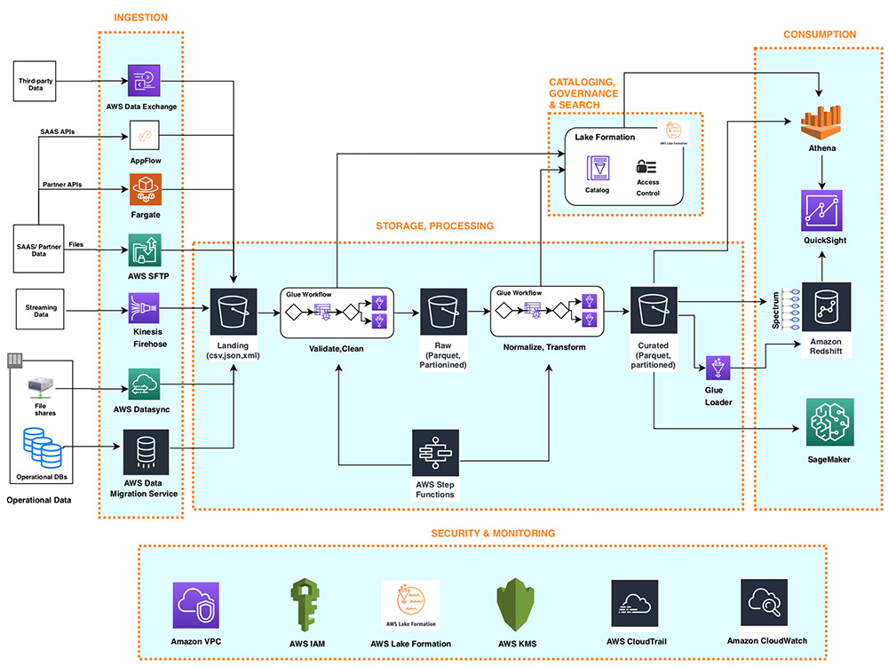
Ingestion layer
The ingestion layer in our serverless architecture is composed of a set of purpose-built AWS services to enable data ingestion from a variety of sources. Each of these services enables simple self-service data ingestion into the data lake landing zone and provides integration with other AWS services in the storage and security layers. Individual purpose-built AWS services match the unique connectivity, data format, data structure, and data velocity requirements of operational database sources, streaming data sources, and file sources.
Operational database sources
Typically, organizations store their operational data in various relational and NoSQL databases. AWS Data Migration Service (AWS DMS) can connect to a variety of operational RDBMS and NoSQL databases and ingest their data into Amazon Simple Storage Service (Amazon S3) buckets in the data lake landing zone. With AWS DMS, you can first perform a one-time import of the source data into the data lake and replicate ongoing changes happening in the source database. AWS DMS encrypts S3 objects using AWS Key Management Service (AWS KMS) keys as it stores them in the data lake. AWS DMS is a fully managed, resilient service and provides a wide choice of instance sizes to host database replication tasks.
AWS Lake Formation provides a scalable, serverless alternative, called blueprints, to ingest data from AWS native or on-premises database sources into the landing zone in the data lake. A Lake Formation blueprint is a predefined template that generates a data ingestion AWS Glue workflow based on input parameters such as source database, target Amazon S3 location, target dataset format, target dataset partitioning columns, and schedule. A blueprint-generated AWS Glue workflow implements an optimized and parallelized data ingestion pipeline consisting of crawlers, multiple parallel jobs, and triggers connecting them based on conditions. For more information, see Integrating AWS Lake Formation with Amazon RDS for SQL Server.
Streaming data sources
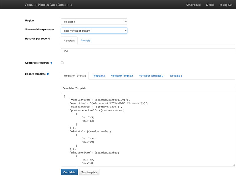
The ingestion layer uses Amazon Kinesis Data Firehose to receive streaming data from internal and external sources. With a few clicks, you can configure a Kinesis Data Firehose API endpoint where sources can send streaming data such as clickstreams, application and infrastructure logs and monitoring metrics, and IoT data such as devices telemetry and sensor readings. Kinesis Data Firehose does the following:
- Buffers incoming streams
- Batches, compresses, transforms, and encrypts the streams
- Stores the streams as S3 objects in the landing zone in the data lake
Kinesis Data Firehose natively integrates with the security and storage layers and can deliver data to Amazon S3, Amazon Redshift, and Amazon Elasticsearch Service (Amazon ES) for real-time analytics use cases. Kinesis Data Firehose is serverless, requires no administration, and has a cost model where you pay only for the volume of data you transmit and process through the service. Kinesis Data Firehose automatically scales to adjust to the volume and throughput of incoming data.
File sources
Many applications store structured and unstructured data in files that are hosted on Network Attached Storage (NAS) arrays. Organizations also receive data files from partners and third-party vendors. Analyzing data from these file sources can provide valuable business insights.
Internal file shares
AWS DataSync can ingest hundreds of terabytes and millions of files from NFS and SMB enabled NAS devices into the data lake landing zone. DataSync automatically handles scripting of copy jobs, scheduling and monitoring transfers, validating data integrity, and optimizing network utilization. DataSync can perform one-time file transfers and monitor and sync changed files into the data lake. DataSync is fully managed and can be set up in minutes.
Partner data files
FTP is most common method for exchanging data files with partners. The AWS Transfer Family is a serverless, highly available, and scalable service that supports secure FTP endpoints and natively integrates with Amazon S3. Partners and vendors transmit files using SFTP protocol, and the AWS Transfer Family stores them as S3 objects in the landing zone in the data lake. The AWS Transfer Family supports encryption using AWS KMS and common authentication methods including AWS Identity and Access Management (IAM) and Active Directory.
Data APIs
Organizations today use SaaS and partner applications such as Salesforce, Marketo, and Google Analytics to support their business operations. Analyzing SaaS and partner data in combination with internal operational application data is critical to gaining 360-degree business insights. Partner and SaaS applications often provide API endpoints to share data.
SaaS APIs
The ingestion layer uses AWS AppFlow to easily ingest SaaS applications data into the data lake. With a few clicks, you can set up serverless data ingestion flows in AppFlow. Your flows can connect to SaaS applications (such as SalesForce, Marketo, and Google Analytics), ingest data, and store it in the data lake. You can schedule AppFlow data ingestion flows or trigger them by events in the SaaS application. Ingested data can be validated, filtered, mapped and masked before storing in the data lake. AppFlow natively integrates with authentication, authorization, and encryption services in the security and governance layer.
Partner APIs
To ingest data from partner and third-party APIs, organizations build or purchase custom applications that connect to APIs, fetch data, and create S3 objects in the landing zone by using AWS SDKs. These applications and their dependencies can be packaged into Docker containers and hosted on AWS Fargate. Fargate is a serverless compute engine for hosting Docker containers without having to provision, manage, and scale servers. Fargate natively integrates with AWS security and monitoring services to provide encryption, authorization, network isolation, logging, and monitoring to the application containers.
AWS Glue Python shell jobs also provide serverless alternative to build and schedule data ingestion jobs that can interact with partner APIs by using native, open-source, or partner-provided Python libraries. AWS Glue provides out-of-the-box capabilities to schedule singular Python shell jobs or include them as part of a more complex data ingestion workflow built on AWS Glue workflows.
Third-party data sources
Your organization can gain a business edge by combining your internal data with third-party datasets such as historical demographics, weather data, and consumer behavior data. AWS Data Exchange provides a serverless way to find, subscribe to, and ingest third-party data directly into S3 buckets in the data lake landing zone. You can ingest a full third-party dataset and then automate detecting and ingesting revisions to that dataset. AWS Data Exchange is serverless and lets you find and ingest third-party datasets with a few clicks.
Storage layer
Amazon S3 provides the foundation for the storage layer in our architecture. Amazon S3 provides virtually unlimited scalability at low cost for our serverless data lake. Data is stored as S3 objects organized into landing, raw, and curated zone buckets and prefixes. Amazon S3 encrypts data using keys managed in AWS KMS. IAM policies control granular zone-level and dataset-level access to various users and roles. Amazon S3 provides 99.99 % of availability and 99.999999999 % of durability, and charges only for the data it stores. To significantly reduce costs, Amazon S3 provides colder tier storage options called Amazon S3 Glacier and S3 Glacier Deep Archive. To automate cost optimizations, Amazon S3 provides configurable lifecycle policies and intelligent tiering options to automate moving older data to colder tiers. AWS services in our ingestion, cataloging, processing, and consumption layers can natively read and write S3 objects. Additionally, hundreds of third-party vendor and open-source products and services provide the ability to read and write S3 objects.
Data of any structure (including unstructured data) and any format can be stored as S3 objects without needing to predefine any schema. This enables services in the ingestion layer to quickly land a variety of source data into the data lake in its original source format. After the data is ingested into the data lake, components in the processing layer can define schema on top of S3 datasets and register them in the cataloging layer. Services in the processing and consumption layers can then use schema-on-read to apply the required structure to data read from S3 objects. Datasets stored in Amazon S3 are often partitioned to enable efficient filtering by services in the processing and consumption layers.
Cataloging and search layer
A data lake typically hosts a large number of datasets, and many of these datasets have evolving schema and new data partitions. A central Data Catalog that manages metadata for all the datasets in the data lake is crucial to enabling self-service discovery of data in the data lake. Additionally, separating metadata from data into a central schema enables schema-on-read for the processing and consumption layer components.
In our architecture, Lake Formation provides the central catalog to store and manage metadata for all datasets hosted in the data lake. Organizations manage both technical metadata (such as versioned table schemas, partitioning information, physical data location, and update timestamps) and business attributes (such as data owner, data steward, column business definition, and column information sensitivity) of all their datasets in Lake Formation. Services such as AWS Glue, Amazon EMR, and Amazon Athena natively integrate with Lake Formation and automate discovering and registering dataset metadata into the Lake Formation catalog. Additionally, Lake Formation provides APIs to enable metadata registration and management using custom scripts and third-party products. AWS Glue crawlers in the processing layer can track evolving schemas and newly added partitions of datasets in the data lake, and add new versions of corresponding metadata in the Lake Formation catalog.
Lake Formation provides the data lake administrator a central place to set up granular table- and column-level permissions for databases and tables hosted in the data lake. After Lake Formation permissions are set up, users and groups can access only authorized tables and columns using multiple processing and consumption layer services such as Athena, Amazon EMR, AWS Glue, and Amazon Redshift Spectrum.
Processing layer
The processing layer in our architecture is composed of two types of components:
- Components used to create multi-step data processing pipelines
- Components to orchestrate data processing pipelines on schedule or in response to event triggers (such as ingestion of new data into the landing zone)
AWS Glue and AWS Step Functions provide serverless components to build, orchestrate, and run pipelines that can easily scale to process large data volumes. Multi-step workflows built using AWS Glue and Step Functions can catalog, validate, clean, transform, and enrich individual datasets and advance them from landing to raw and raw to curated zones in the storage layer.
AWS Glue is a serverless, pay-per-use ETL service for building and running Python or Spark jobs (written in Scala or Python) without requiring you to deploy or manage clusters. AWS Glue automatically generates the code to accelerate your data transformations and loading processes. AWS Glue ETL builds on top of Apache Spark and provides commonly used out-of-the-box data source connectors, data structures, and ETL transformations to validate, clean, transform, and flatten data stored in many open-source formats such as CSV, JSON, Parquet, and Avro. AWS Glue ETL also provides capabilities to incrementally process partitioned data.
Additionally, you can use AWS Glue to define and run crawlers that can crawl folders in the data lake, discover datasets and their partitions, infer schema, and define tables in the Lake Formation catalog. AWS Glue provides more than a dozen built-in classifiers that can parse a variety of data structures stored in open-source formats. AWS Glue also provides triggers and workflow capabilities that you can use to build multi-step end-to-end data processing pipelines that include job dependencies and running parallel steps. You can schedule AWS Glue jobs and workflows or run them on demand. AWS Glue natively integrates with AWS services in storage, catalog, and security layers.
Step Functions is a serverless engine that you can use to build and orchestrate scheduled or event-driven data processing workflows. You use Step Functions to build complex data processing pipelines that involve orchestrating steps implemented by using multiple AWS services such as AWS Glue, AWS Lambda, Amazon Elastic Container Service (Amazon ECS) containers, and more. Step Functions provides visual representations of complex workflows and their running state to make them easy to understand. It manages state, checkpoints, and restarts of the workflow for you to make sure that the steps in your data pipeline run in order and as expected. Built-in try/catch, retry, and rollback capabilities deal with errors and exceptions automatically.
Consumption layer
The consumption layer in our architecture is composed using fully managed, purpose-built, analytics services that enable interactive SQL, BI dashboarding, batch processing, and ML.
Interactive SQL
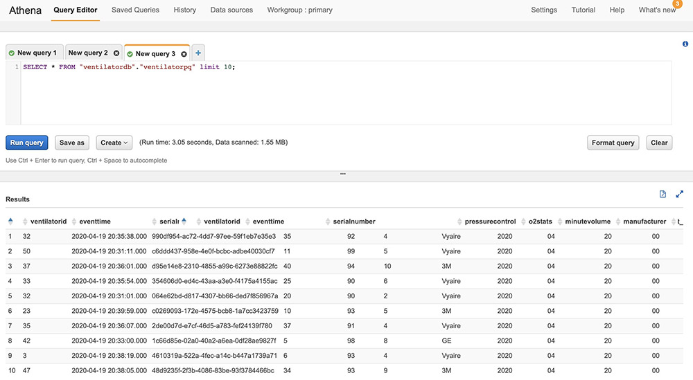
Athena is an interactive query service that enables you to run complex ANSI SQL against terabytes of data stored in Amazon S3 without needing to first load it into a database. Athena queries can analyze structured, semi-structured, and columnar data stored in open-source formats such as CSV, JSON, XML Avro, Parquet, and ORC. Athena uses table definitions from Lake Formation to apply schema-on-read to data read from Amazon S3.
Athena is serverless, so there is no infrastructure to set up or manage, and you pay only for the amount of data scanned by the queries you run. Athena provides faster results and lower costs by reducing the amount of data it scans by using dataset partitioning information stored in the Lake Formation catalog. You can run queries directly on the Athena console of submit them using Athena JDBC or ODBC endpoints.
Athena natively integrates with AWS services in the security and monitoring layer to support authentication, authorization, encryption, logging, and monitoring. It supports table- and column-level access controls defined in the Lake Formation catalog.
Data warehousing and batch analytics
Amazon Redshift is a fully managed data warehouse service that can host and process petabytes of data and run thousands highly performant queries in parallel. Amazon Redshift uses a cluster of compute nodes to run very low-latency queries to power interactive dashboards and high-throughput batch analytics to drive business decisions. You can run Amazon Redshift queries directly on the Amazon Redshift console or submit them using the JDBC/ODBC endpoints provided by Amazon Redshift.
Amazon Redshift provides the capability, called Amazon Redshift Spectrum, to perform in-place queries on structured and semi-structured datasets in Amazon S3 without needing to load it into the cluster. Amazon Redshift Spectrum can spin up thousands of query-specific temporary nodes to scan exabytes of data to deliver fast results. Organizations typically load most frequently accessed dimension and fact data into an Amazon Redshift cluster and keep up to exabytes of structured, semi-structured, and unstructured historical data in Amazon S3. Amazon Redshift Spectrum enables running complex queries that combine data in a cluster with data on Amazon S3 in the same query.
Amazon Redshift provides native integration with Amazon S3 in the storage layer, Lake Formation catalog, and AWS services in the security and monitoring layer.
Business intelligence
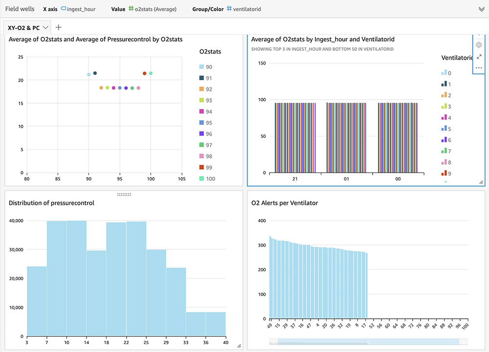
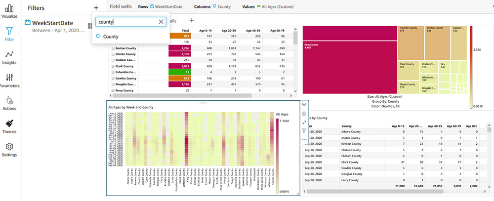
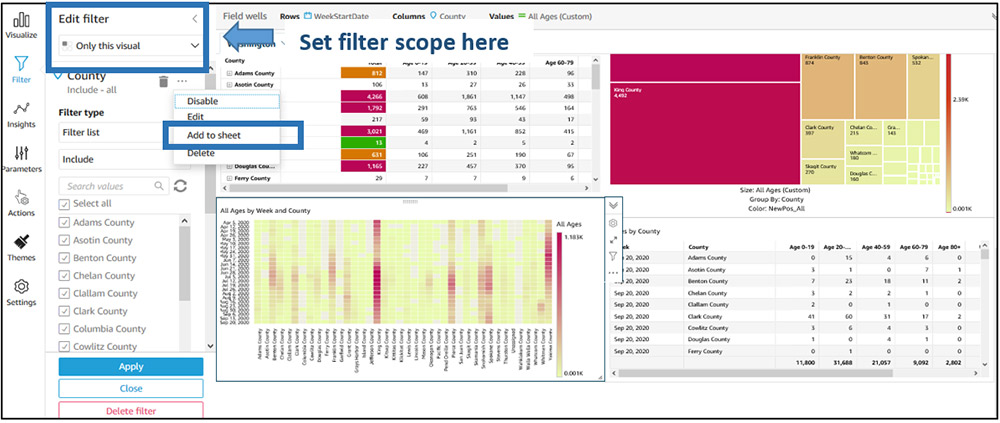
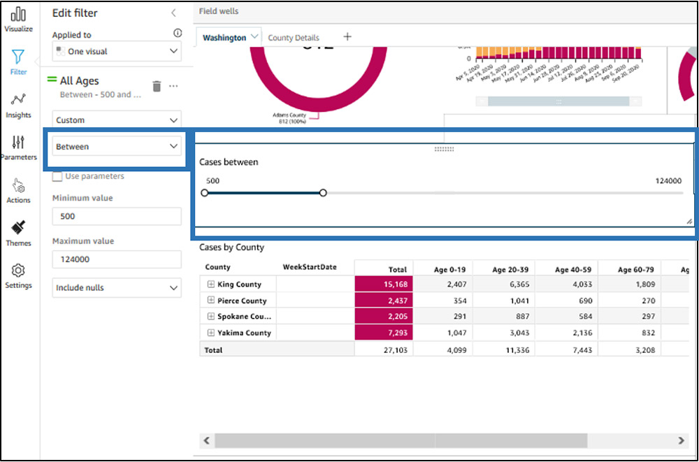
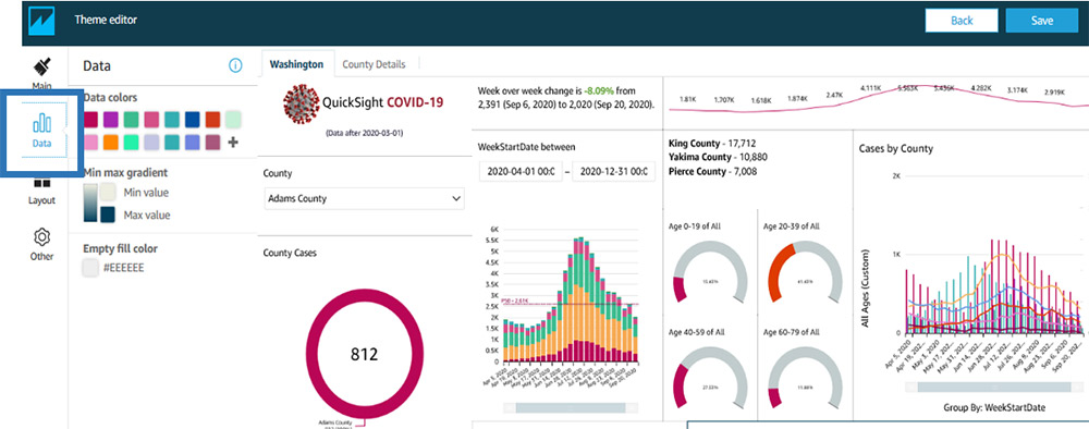
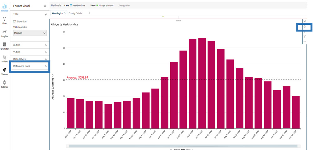
Amazon QuickSight provides a serverless BI capability to easily create and publish rich, interactive dashboards. QuickSight enriches dashboards and visuals with out-of-the-box, automatically generated ML insights such as forecasting, anomaly detection, and narrative highlights. QuickSight natively integrates with Amazon SageMaker to enable additional custom ML model-based insights to your BI dashboards. You can access QuickSight dashboards from any device using a QuickSight app, or you can embed the dashboard into web applications, portals, and websites.
QuickSight allows you to directly connect to and import data from a wide variety of cloud and on-premises data sources. These include SaaS applications such as Salesforce, Square, ServiceNow, Twitter, GitHub, and JIRA; third-party databases such as Teradata, MySQL, Postgres, and SQL Server; native AWS services such as Amazon Redshift, Athena, Amazon S3, Amazon Relational Database Service (Amazon RDS), and Amazon Aurora; and private VPC subnets. You can also upload a variety of file types including XLS, CSV, JSON, and Presto.
To achieve blazing fast performance for dashboards, QuickSight provides an in-memory caching and calculation engine called SPICE. SPICE automatically replicates data for high availability and enables thousands of users to simultaneously perform fast, interactive analysis while shielding your underlying data infrastructure. QuickSight automatically scales to tens of thousands of users and provides a cost-effective, pay-per-session pricing model.
QuickSight allows you to securely manage your users and content via a comprehensive set of security features, including role-based access control, active directory integration, AWS CloudTrail auditing, single sign-on (IAM or third-party), private VPC subnets, and data backup.
Predictive analytics and ML
Amazon SageMaker is a fully managed service that provides components to build, train, and deploy ML models using an interactive development environment (IDE) called Amazon SageMaker Studio. In Amazon SageMaker Studio, you can upload data, create new notebooks, train and tune models, move back and forth between steps to adjust experiments, compare results, and deploy models to production, all in one place by using a unified visual interface. Amazon SageMaker also provides managed Jupyter notebooks that you can spin up with just a few clicks. Amazon SageMaker notebooks provide elastic compute resources, git integration, easy sharing, pre-configured ML algorithms, dozens of out-of-the-box ML examples, and AWS Marketplace integration, which enables easy deployment of hundreds of pre-trained algorithms. Amazon SageMaker notebooks are preconfigured with all major deep learning frameworks, including TensorFlow, PyTorch, Apache MXNet, Chainer, Keras, Gluon, Horovod, Scikit-learn, and Deep Graph Library.
ML models are trained on Amazon SageMaker managed compute instances, including highly cost-effective Amazon Elastic Compute Cloud (Amazon EC2) Spot Instances. You can organize multiple training jobs by using Amazon SageMaker Experiments. You can build training jobs using Amazon SageMaker built-in algorithms, your custom algorithms, or hundreds of algorithms you can deploy from AWS Marketplace. Amazon SageMaker Debugger provides full visibility into model training jobs. Amazon SageMaker also provides automatic hyperparameter tuning for ML training jobs.
You can deploy Amazon SageMaker trained models into production with a few clicks and easily scale them across a fleet of fully managed EC2 instances. You can choose from multiple EC2 instance types and attach cost-effective GPU-powered inference acceleration. After the models are deployed, Amazon SageMaker can monitor key model metrics for inference accuracy and detect any concept drift.
Amazon SageMaker provides native integrations with AWS services in the storage and security layers.
Security and governance layer
Components across all layers of our architecture protect data, identities, and processing resources by natively using the following capabilities provided by the security and governance layer.
Authentication and authorization
IAM provides user-, group-, and role-level identity to users and the ability to configure fine-grained access control for resources managed by AWS services in all layers of our architecture. IAM supports multi-factor authentication and single sign-on through integrations with corporate directories and open identity providers such as Google, Facebook, and Amazon.
Lake Formation provides a simple and centralized authorization model for tables hosted in the data lake. After implemented in Lake Formation, authorization policies for databases and tables are enforced by other AWS services such as Athena, Amazon EMR, QuickSight, and Amazon Redshift Spectrum. In Lake Formation, you can grant or revoke database-, table-, or column-level access for IAM users, groups, or roles defined in the same account hosting the Lake Formation catalog or another AWS account. The simple grant/revoke-based authorization model of Lake Formation considerably simplifies the previous IAM-based authorization model that relied on separately securing S3 data objects and metadata objects in the AWS Glue Data Catalog.
Encryption
AWS KMS provides the capability to create and manage symmetric and asymmetric customer-managed encryption keys. AWS services in all layers of our architecture natively integrate with AWS KMS to encrypt data in the data lake. It supports both creating new keys and importing existing customer keys. Access to the encryption keys is controlled using IAM and is monitored through detailed audit trails in CloudTrail.
Network protection
Our architecture uses Amazon Virtual Private Cloud (Amazon VPC) to provision a logically isolated section of the AWS Cloud (called VPC) that is isolated from the internet and other AWS customers. AWS VPC provides the ability to choose your own IP address range, create subnets, and configure route tables and network gateways. AWS services from other layers in our architecture launch resources in this private VPC to protect all traffic to and from these resources.
Monitoring and logging
AWS services in all layers of our architecture store detailed logs and monitoring metrics in AWS CloudWatch. CloudWatch provides the ability to analyze logs, visualize monitored metrics, define monitoring thresholds, and send alerts when thresholds are crossed.
All AWS services in our architecture also store extensive audit trails of user and service actions in CloudTrail. CloudTrail provides event history of your AWS account activity, including actions taken through the AWS Management Console, AWS SDKs, command line tools, and other AWS services. This event history simplifies security analysis, resource change tracking, and troubleshooting. In addition, you can use CloudTrail to detect unusual activity in your AWS accounts. These capabilities help simplify operational analysis and troubleshooting.
Additional considerations
In this post, we talked about ingesting data from diverse sources and storing it as S3 objects in the data lake and then using AWS Glue to process ingested datasets until they’re in a consumable state. This architecture enables use cases needing source-to-consumption latency of a few minutes to hours. In a future post, we will evolve our serverless analytics architecture to add a speed layer to enable use cases that require source-to-consumption latency in seconds, all while aligning with the layered logical architecture we introduced.
Conclusion
With AWS serverless and managed services, you can build a modern, low-cost data lake centric analytics architecture in days. A decoupled, component-driven architecture allows you to start small and quickly add new purpose-built components to one of six architecture layers to address new requirements and data sources.
We invite you to read the following posts that contain detailed walkthroughs and sample code for building the components of the serverless data lake centric analytics architecture:
- Load ongoing data lake changes with AWS DMS and AWS Glue
- Discover metadata with AWS Lake Formation: Part 1 and Part 2
- Build a Data Lake Foundation with AWS Glue and Amazon S3
- Process data with varying data ingestion frequencies using AWS Glue job bookmarks
- Orchestrate Amazon Redshift-Based ETL workflows with AWS Step Functions and AWS Glue
- Analyze your Amazon S3 spend using AWS Glue and Amazon Redshift
- From Data Lake to Data Warehouse: Enhancing Customer 360 with Amazon Redshift Spectrum
- Extract, Transform and Load data into S3 data lake using CTAS and INSERT INTO statements in Amazon Athena
- Derive Insights from IoT in Minutes using AWS IoT, Amazon Kinesis Firehose, Amazon Athena, and Amazon QuickSight
- Our data lake story: How Woot.com built a serverless data lake on AWS
- Predicting all-cause patient readmission risk using AWS data lake and machine learning
About the Authors
 Praful Kava is a Sr. Specialist Solutions Architect at AWS. He guides customers to design and engineer Cloud scale Analytics pipelines on AWS. Outside work, he enjoys travelling with his family and exploring new hiking trails.
 Changbin Gong is a Senior Solutions Architect at Amazon Web Services (AWS). He engages with customers to create innovative solutions that address customer business problems and accelerate the adoption of AWS services. In his spare time, Changbin enjoys reading, running, and traveling.
 Kaushik Krishnamurthi is a Senior Data Engineer at Amazon Web Services (AWS), where he focuses on building scalable platforms for business analytics and machine learning. Prior to AWS, he worked in several business intelligence and data engineering roles for many years.
 Gagan Brahmi is a Specialist Solutions Architect focused on Big Data & Analytics at Amazon Web Services. Gagan has over 15 years of experience in information technology. He helps customers architect and build highly scalable, performant, and secure cloud-based solutions on AWS.
 Juan Yu is a Data Warehouse Specialist Solutions Architect at Amazon Web Services, where she helps customers adopt cloud data warehouses and solve analytic challenges at scale. Prior to AWS, she had fun building and enhancing MPP query engines to improve customer experience on Big Data workloads.
 Ran Sheinberg is a principal solutions architect in the EC2 Spot team with Amazon Web Services. He works with AWS customers on cost optimizing their compute spend by utilizing Spot Instances across different types of workloads: stateless web applications, queue workers, containerized workloads, analytics, HPC and others.


 Neeraja Rentachintala is a Principal Product Manager with Amazon Redshift. Neeraja is a seasoned Product Management and GTM leader, bringing over 20 years of experience in product vision, strategy and leadership roles in data products and platforms. Neeraja delivered products in analytics, databases, data Integration, application integration, AI/Machine Learning, large scale distributed systems across On-Premise and Cloud, serving Fortune 500 companies as part of ventures including MapR (acquired by HPE), Microsoft SQL Server, Oracle, Informatica and Expedia.com.
 Jenny Chen is a senior database engineer at Amazon Redshift focusing on all aspects of Redshift performance, like Query Processing, Concurrency, Distributed system, Storage, OS and many more. She works together with development team to ensure of delivering highest performance, scalable and easy-of-use database for customer. Prior to her career in cloud data warehouse, she has 10-year of experience in enterprise database DB2 for z/OS in IBM with focus on query optimization, query performance and system performance.
 Suzhen Lin is a senior software development engineer on the Amazon Redshift transaction processing and storage team. Suzhen Lin has over 15 years of experiences in industry leading analytical database products including AWS Redshift, Gauss MPPDB, Azure SQL Data Warehouse and Teradata as senior architect and developer. Her experiences cover storage, transaction processing, query processing, memory/disk caching and etc in on-premise/cloud database management systems.


 Amir Bar Or is a Principal Data Architect at AWS Professional Services. After 20 years leading software organizations and developing data analytics platforms and products, he is now sharing his experience with large enterprise customers and helping them scale their data analytics in the cloud.
 Dr. Aaron Friedman a Principal Solutions Architect at Amazon Web Services working with healthcare and life sciences startups to accelerate science and improve patient care. His passion is working at the intersection of science, big data, and software. Outside of work, he’s with his family outdoors or learning a new thing to cook.


 Mohammed “Afsar ” Jahangir Ali is a Senior Big Data Consultant with Amazon since January 2018. He is a data enthusiast helping customers shape their data lakes and analytic journeys on AWS.In his spare time, he enjoys taking pictures, listening to music, and spend time with family.
 Wendy Neu has worked as a Data Architect with Amazon since January 2015. Prior to joining Amazon, she worked as a consultant in Cincinnati, OH helping customers integrate and manage their data from different unrelated data sources.


 Rob Craig is a Senior Solutions Architect with AWS. He supports customers in the UK with their cloud journey, providing them with architectural advice and guidance to help them achieve their business outcomes.
 Dylan Qu is an AWS solutions architect responsible for providing architectural guidance across the full AWS stack with a focus on Data Analytics, AI/ML and DevOps.


 Ying Wang is a Data Visualization Engineer with the Data & Analytics Global Specialty Practice in AWS Professional Services.


 Satya Vajrapu is a DevOps Consultant with Amazon Web Services. He works with AWS customers to help design and develop various practices and tools in the DevOps toolchain.
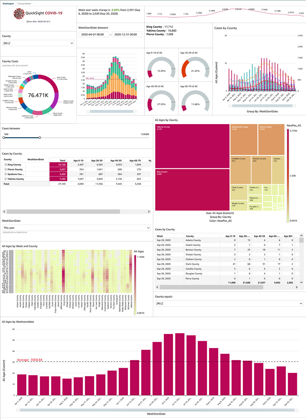


 Jose Kunnackal John is a principal product manager for Amazon QuickSight.
 Sahitya Pandiri is a technical program manager with Amazon Web Services. Sahitya has been in product/program management for 6 years now, and has built multiple products in the retail, healthcare, and analytics space.
 Chirag Dhull is a Principal Product Marketing Manager for Amazon QuickSight.
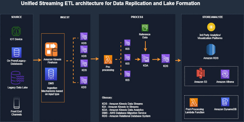
 Ram Vittal is an enterprise solutions architect at AWS. His current focus is to help enterprise customers with their cloud adoption and optimization journey to improve their business outcomes. In his spare time, he enjoys tennis, photography, and movies.
 Akash Bhatia is a Sr. solutions architect at AWS. His current focus is helping customers achieve their business outcomes through architecting and implementing innovative and resilient solutions at scale.

 Vijay Injam is a Data Architect with Amazon Web Services.
  Kevin Fallis is an AWS specialist search solutions architect. His passion at AWS is to help customers leverage the correct mix of AWS services to achieve success for their business goals. His after-work activities include family, DIY projects, carpentry, playing drums, and all things music.


 Adnan Hasan is a Global GTM Analytics Specialist at Amazon Web Services, helping customers transform their business using data, machine learning and advanced analytics.