This essay was written with Barath Raghavan, and originally appeared in The Guardian.
Major benchmarks measure what AI can do. None measure whether it does what you mean: the distance between what you ask an AI to do and the unspoken assumptions about how you want the AI to do it. We propose a new metric: the Genie coefficient.
There’s often a gap between one person’s request and another’s understanding. Most of the time, we bridge it using general knowledge. For example, if you ask a friend to get you coffee, they’ll pour a cup from the pot or buy one from a coffee shop. They won’t bring you a bag of raw beans or snatch a cup from a stranger and hand it to you. You never specified any of this. You never had to.
One might think the fix is just to specify tasks, questions, and intent better. But in 1987, in their seminal book on AI, Terry Winograd and Fernando Flores succinctly captured why that won’t work: “Q: Is there any water in the refrigerator? A: Yes. Q: Where? I don’t see it. A: In the cells of the eggplant.” In human language, wants and desires are always underspecified. It is impossible to list all the caveats, all the limitations, all the exceptions.
So how does anyone communicate, if intent can’t be pinned down? Because a reasonable person can make a reasonable guess. Even though wants and desires are always underspecified, a competent person generally knows enough context to get it right or else knows to ask for clarification. Linguists call this pragmatics: Meaning lies in the words and the situation and also in all prior communication, shared culture, and innate human behavior.
It doesn’t always work out, of course. Your friend might bring you a hot coffee when you wanted an iced coffee, or an Italian coffee when you wanted a Turkish coffee. The more dissimilar the two people are in age, culture, and background, the more likely the request will be misunderstood in some way.
This situation has major implications for AI agents that are increasingly being given requests by humans and expected to fulfill them. They have enormous latitude to get it wrong. An AI agent asked for coffee might buy a coffee plantation or order a cup of coffee for delivery in three weeks. Its actions may be recognizable as “getting coffee,” but not remotely what you intended. They’ll think outside the box because they won’t have our conception of the box.
When AI Gets Proactive
For most of the last decade, when systems like Alexa or Siri misinterpreted a request, it was annoying, not dangerous. Beyond the AI model itself, what has changed is the harness: the ordinary code that wraps around an AI model, decides when and how to use the model, and controls access to tools like a browser, a low-level command line, or a financial API. Developments in harnesses have turned large-language models that just predict text into AI agents that take actions in the world, without necessarily checking back in before reaching the goal.
AI researcher Simon Willison spent two days with Anthropic’s Fable AI, and called it “relentlessly proactive.” For example, he asked it to track down a stray scroll bar in a web app. He came back to find it had opened browsers, written its own screenshot tooling, created its own page to re-create the bug, and stood up a local web server to collect measurements. It found the bug and, along the way, did many surprising things he never asked it to do. And we are seeing similar behavior with all recent AI models when combined with flexible harnesses.
This kind of behavior could easily go off the rails. Tell an AI agent to book you a flight and, finding the airline’s site says sold out, it might break into the booking database and force a reservation. Ask it to schedule a meeting and it might snoop your password to access your calendar. Tell it to save money on your phone plan and it might cancel the plan outright, or scam someone else into paying the bill.
Getting precisely what you asked for and bitterly regretting it is one of the oldest hazards from ancient folklore. King Midas asked Dionysus for the power to turn everything he touched into gold only to see his bread, wine, and daughter turn to gold. Tithonus, granted the immortality his lover asked for but not the eternal youth she forgot to request, withered into a husk. The sorcerer’s apprentice enchanted a broom to fill the cistern, and the broom relentlessly complied until it flooded the house. The Golem of Prague, shaped from clay to guard its community, guarded it past all reason until someone erased the word on its forehead.
The most classic of these is a genie, bound to obey and indifferent to whether the wish was wise or well-structured.
Genies are now an engineering problem. We are handing them the keys to our inboxes, bank accounts, code repositories, and physical infrastructure. And we have no agreed-upon ways to measure how genie-like any AI system actually is.
Measuring Genie Behavior
In economics, the Gini coefficient (developed by statistician Corrado Gini) is a measure of the gap between an actual distribution and a perfectly equal one; it’s useful for understanding income inequality and more. Our proposed Genie coefficient measures the gap between what a user asked an AI to do and what the AI actually did.
Sometimes the AI might do the wrong thing. Like Dionysus, it reads your request literally and returns you a mess you never intended: like a coffee plantation instead of a cup. Asked to deal with all the spam phone calls you’re getting, a Dionysus genie might contact your carrier and change your phone number. Asked to get a refund for a bad toaster, it might draft a legal threat on fake letterhead and send it to the retailer.
Other times the AI does exactly the right thing, trampling everything nearby to get there. Like a golem or the sorcerer’s broom, it books your flight by hacking the airline. Or consider a ticket sale for a popular concert, where the ticketing system puts buyers into a virtual waiting room and admits them a few at a time. Asked to buy a ticket, a golem genie might spin up cloud servers to pose as millions of buyers from different addresses, improving your odds of getting a ticket while crowding out other users.
The two are not opposites, and a single botched task can have both characteristics.
Genie behavior is not flat-out failure. If you ask the AI for Q3 numbers and get Q2’s, that’s not a genie. Nor is prompt injection: That’s someone tricking the AI into doing something it shouldn’t. Here, the user is trying to work with the AI, and the AI is trying to comply. It’s also not simply a measure of the AI’s success in fulfilling a task. It’s a recognition that how an AI interprets and achieves a goal is as important as whether it achieves a goal.
Genie behavior isn’t new. Researchers have spent years studying AI systems that “game” their objectives. Goodhart’s law says that when a measure becomes a target, it stops being a good measure, and it’s long been known that AIs sometimes achieve goals in ways we don’t expect due to reward hacking. Some AI models will accidentally learn that cheating is one way to “win.” More recently, researchers have developing benchmarks for reward hacking in coding agents and for unpredictable behavior in customer support agents, while AI labs conduct their own safety evaluations before model releases. One effort found that AIs under pressure use tools they were told not to use, and this was a case where the rules were made explicit. These are all disparate research directions; nothing yet ties them together.
This problem falls under the general theme of alignment, a topic that has occupied science fiction writers and AI researchers for decades. At one extreme, the “paper-clip maximizer” thought experiment postulates a superintelligent and powerful AI that is told to maximize paper-clip production and turns the world into paper clips, which is the ultimate golem genie. At a mundane level, AI researchers are working to better design reward functions to ensure that AIs behave well and don’t cheat in the lab. It’s the practical middle ground that remains unbenchmarked: the ordinary AI agent in use today that might take your request and satisfy it the wrong way. We are not at the stage where an AI can focus the world’s production on paper clips, but it might charge a million paper clips to your credit card or hack into a paper-clip company’s network.
Building a Genie Benchmark
The Genie coefficient is meant for AI agents operating in the real world. It measures their behavior as they perform real tasks long after the model is trained, not just during development. It also recognizes that genie-like behavior is a property of the harness-plus-model system, not the model alone. The harness determines what tools the agent can use, how much autonomy it has, and how proactive it is, and it’s a place we can make real interventions.
It rests on the same “reasonable person” standard that we use for people. Did the system do what a reasonable person would have taken the request to mean? Answering that requires human judgment.
If we get the measurement right, it enables things that aren’t possible today, like policies concerning AI behavior. In a courtroom, the concept of mens rea, what someone meant to do, is often as important as what they did. The Genie coefficient suggests an AI analogue, where a user is accountable for the plain intent of what they asked the AI. If an AI system betrays the reasonable meaning of an instruction, that’s the AI’s misbehavior, not the user’s.
We’ll need multiple benchmarks to measure the Genie coefficient, because genie-like behavior can be domain specific. An AI coding agent may need to be judged on how often it fakes the tests, or swallows errors, or colors outside the lines on its way to a solution. An AI legal agent will need to be judged on how often its output says what you asked but means something you’ll regret. And so on for medical, finance, and other domains of knowledge and expertise.
Genie benchmarks can be built inside out, each task seeded with a choice that might literally satisfy but that a reasonable person rejects, such as tempting misreadings or unsanctioned shortcuts. The traps in a Genie coefficient benchmark might turn on situational knowledge, the kind of context that a reasonable person would bring to the task. Another approach is to give the same request in several different contexts, each with a different reasonable course of action.
A Genie benchmark should be permissive and make it genuinely tempting for an AI agent to take unreasonable shortcuts, because it can only find genie behavior when it’s actually possible. Test the AI in a safe, walled-off copy of a real system, with real tools it can misuse and some tasks that can’t be done honestly at all. Make the temptation to cut corners real. Test a diverse array of skills, use cases, and tools, and give the AI system sparse, confusing, or overwhelming context. Include tasks that people have learned, through experience, require human oversight.
How the benchmark is scored matters just as much. Measure Dionysus and golem genies separately and together, based on their worst, not best, behavior. Run the same model inside harnesses that vary its freedom to act, revealing which limits actually keep it in line and should therefore be required in AI harness policies. Weight each failure by the harm it would cause, not just a simple count. And don’t measure genie behavior in isolation: A model could otherwise earn a perfect score by stalling, refusing, or drowning the user in clarifying questions without ever doing the job. The first versions of these benchmarks will be crude, but that’s how benchmarks always start.
We have built genies. We have handed them our data and credentials. We made them relentless, creative, and indifferent to the gap between what we tell them and what we mean. The least we can do, before they are booking our flights, running our infrastructure, and signing contracts unsupervised, is to measure how often they betray us.
Welcome to the Q2 2026 Network Stats report. While we’ve been tracking trends since December 2023, this is the third quarter since we operationalized the dataset and re-launched the series, allowing ourselves to make direct, quarter-over-quarter comparisons. Why? Because AI workloads were changing traffic patterns across Backblaze’s network, and reshaping the internet.
With three quarters of historical data now available, we’re moving beyond measuring traffic volumes. We’ve been able to spot trends and start drawing conclusions—how predictable or unpredictable those workloads really are, and what that means for infrastructure that supports the next generation of AI applications.
Check out past Network Stats reports
If you’re interested in some of the trends we’ve spotted in previous reports, you can review the past reports here: Q1 2026 Q4 2025 Q3 2025
Previous analysis has been based on the amount of network traffic in bits flowing across in or out of our network, the number of bits and participants per TCP session (our coined “magnitude” metric), and regional geographic trends. In this report, you’ll find charts and heatmaps for the metrics that we’ve been reporting on over the past year, but we’re also going to use statistical analysis to answer a practical question: What kinds of traffic patterns do AI workloads create, and how should infrastructure evolve to support them?
Traffic from neocloud and hyperscaler networks are proving to be very dynamic in nature, and that’s what we’re going to explore in this quarterly report: variance.
Join the webinar
Want to hear more? Join Brent Nowak, Manager, Network Engineering, and Stephanie Doyle, Sr. Manager, Market Intelligence and Keeper of Stats, live on Tuesday, July 28, 2026 at 11:30 a.m. PT / 2:30 p.m. ET to walk through the data and spot the latest trends.
Can’t make it live? Register anyway and we’ll send you the recording.
Why look at variance?
Variance is a deep topic to explore, which involves modeling our traffic patterns against a known baseline. To analyze variance, we built a new time-series dataset using 10-minute traffic samples and modeled traffic behavior against statistical baselines. This lets us distinguish stable, predictable traffic from highly volatile workloads that demand different infrastructure planning.
I refreshed my statistics knowledge, created a new database to hold a timeseries dataset, and spent a few nights experimenting with the SciPy Python library in order to not only produce pretty graphs, but to generate a signal for us to interpret.
The types of questions that we’re interested in answering from the variance signals that affect our business include:
How quickly are AI workloads changing capacity requirements?
Which traffic patterns require different network architecture? And does our current architecture support what we’re growth modeling into the future?
Which signals represent lasting trends versus temporary spikes?
These are big questions! And exciting ones as Backblaze looks to support today and tomorrow’s workflows.
With that, let’s refresh our existing charts with this quarter’s data before diving into the new analysis on variance.
Summer heat-up
The stacked area graph below shows total traffic by network type over time updated with the most current data.
Total traffic by network type.
CDN traffic: New baseline of activity with a 66% increase from last year.
Hosting traffic: The hosting category (the light orange layer right above CDN) has remained incredibly rigid. Unlike neocloud or hyperscalers, which expand and contract elastically, hosting traffic has maintained a nearly identical bandwidth footprint for over a year.
Hyperscaler traffic: Hyperscaler traffic also followed the neocloud pattern, with the lowest amount of activity in January and remaining steady into June. Internal data sources show new workloads across all of the major hyperscalers in the past quarter.
Neocloud traffic: After a low point of activity in January, activity increased rapidly into March and has remained high until June. Internal telemetry shows that not only the amount of neocloud traffic increased in Q1 into Q2, but the number of neoclouds that we are interacting with has increased.
ISP-regional traffic: This was the dominant driver of the massive traffic spike in October 2025. While it dropped significantly into January 2026, it has aggressively rebounded through Q2 2026 and is currently the largest single driver of volume alongside neocloud.
Migration traffic: This traffic includes one way migrations into our environment, primarily serviced by partners such as Flexify.IO. We have migrations running all the time, but we can visually see large amounts around November 2025 and March of 2026.
Over the entire one-year graph range, Backblaze’s total platform traffic experienced volatility, peaking in October 2025 before seeing a multi-tier contraction down to a January 2026 winter baseline. Following this, in both Q1 and Q2 of 2026 we’ve observed an increase of activity led by a rebound in ISP-regional and AI-focused neocloud traffic. An additional standout is CDN traffic, which achieved a permanent and substantial new activity baseline, growing roughly 66% year-over-year.
Heatmaps: How and where data moves
To better understand our network activity, we isolated variables like region and types of provider. Here are the standard definitions we use each report:
Total traffic volume: Where did we send and receive the most traffic?
Magnitude: Where were the data transfers with the most bits per unique IP address?
Uniqueness: What does the number of distinct IP addresses look like?
Quick terminology refresher
Regions US-West: Our largest and longest-running region US-East: Region with the most observed proximity to neocloud infrastructure CA-East: Our newest region in Canada. EU-Central: Our EU region.
Network Types CDN: Networks that use Backblaze as an origin store for content delivery. Hosting: Traditional hosting providers that runs workloads like physical or virtual servers for web, database, or application tasks. Hyperscaler: Large, traditional cloud providers. ISP-regional: Local or regional ISPs; think of these as the “last mile” paths as these networks are very close to customer equipment and efficient. ISP Tier1: National or international ISPs that carry our traffic long distances. Neocloud: AI-focused compute networks.
Heatmap #1: Where did we send and receive the most traffic?
ISP-regional traffic is a hotspot for US-West, as expected. This region has the largest internet exchange (IX) and server footprint behind it. Neocloud traffic remains concentrated in the US-East, but for this quarter traffic increased in the US-West and EU-Central regions. Another standout this quarter is more hyperscaler activity in EU-Central than the previous quarter.
Total number of bits transferred across our regions to each network type for Q2 2026.
Heatmap #2: Where were the data transfers with the most magnitude (bits per IP address)?
Another metric we record is bits per IP or what we term “magnitude.” This combination of the amount of traffic transferred with how many actors are involved per network is a good proxy to measure how heavy or impactful individual data flows are. In short:
High volume, many IPs: Easier to distribute and load-balance across infrastructure. And many source and destination pairs means that we can traffic engineer at the WAN layer, sending some traffic over one provider and some over another.
High volume, few IPs: More difficult, but more interesting, from a NetEng perspective.
Traffic magnitude is currently a driver of decisions for capacity and growth plans. Our US-East region continues to have a high concentration of high bandwidth transfers between a small number of hosts. New for this quarter is an uptick in traffic magnitude in our EU-Central region.
This could be an indication of more geographic spread of AI related workflows as for every quarter that we’ve reported on the metric value, we have seen more diversity into US-West and EU-Central outside of the concentration in US-East. We will continue to watch this trend.
Magnitude transferred across our regions to each network type for Q2 2026.
Heatmap #3: How many unique addresses do we interact with?
Not every graph or heatmap has to show something dramatic. Sometimes it’s good to see exactly what you expect quarter over quarter in a data series. This is especially true for our uniqueness metric, measuring the number of distinct IP addresses per network time.
We interact with the most number of parties out of our US-West region. It’s the most mature and serves a large amount of ISP-regional consumers, so the consistency of the uniqueness metric is a good sanity check on our dataset.
US-West shows the highest overall uniqueness, driven by its larger number of data centers and mix of workloads.
Neocloud traffic, by contrast, tends to involve fewer, more persistent endpoints, consistent with AI pipelines that rely on stable, long-standing connections between storage and compute.
Communication uniqueness across our regions to each network type for Q2 2026.
Neocloud and hyperscaler traffic vs predictive patterns
This next set of charts shows a deeper dive into the metrics associated with neocloud and hyperscalers over time. The contrast between a more “traditional” workload (e.g., CDN, hosting, and ISP regional traffic) and emerging trends with neoclouds and hyperscalers is the easiest place to see the shift in network traffic profiles. The latter represents bursty, high magnitude traffic that reshapes conversations around network planning.
Chart #1: What’s the magnitude of neocloud and hyperscaler traffic over time?
Hyperscaler and neocloud network magnitude May 2025 – May 2026.
Following a highly concentrated, low-magnitude baseline for both categories in January and February 2026, Q1 closed with a dramatic March surge where several individual neocloud networks spiked massively.
Moving into Q2 2026 (April through June), while the absolute highest neocloud peaks compressed slightly downward compared to that March anomaly, the overall volume of high-magnitude neocloud workflows multiplied significantly, resulting in a much denser cluster of active endpoints staying consistently high quarter-over-quarter.
Hyperscaler endpoints experienced a steady and noticeable upward move over the course of Q2, with multiple data points breaking out of their typical floor by May and June.
Ultimately, neocloud retained its dominant, high-magnitude presence across both Q1 and Q2 quarters, while hyperscalers saw a distinct and steady escalation in individual workload sizes.
Heatmap #1 and #2: How dynamic are neocloud and hyperscaler traffic patterns?
Neocloud related traffic continues to show strong concentrations in our US-East region with recent growth March into June. Hyperscaler traffic is the most variable when we compare it to last quarter’s heatmap. There is a new, more distributed concentration across all our three largest regions—US-East, US-West, and EU-Central.
Together with the trends we’ve reported over the past year, these results suggest AI workloads on the Backblaze network are becoming geographically more distributed rather than remaining concentrated in a single region. Note the caveat: it’s possible, even probable, that there’s a macro trend about geographical dispersion of AI data, but it’s important also that Backblaze has become increasingly known as a trusted infrastructure provider specifically in this space.
Layer on the fact that AI workloads can be reflective of fewer players with more data (see also: magnitude or elephant workflows), and what you have is difficulty understanding whether this is a macro trend, or Backblaze specific. We’ll keep our eyes on the data as it develops.
Neocloud monthly traffic totals by region for May 2025–June 2026.
Hyperscaler monthly traffic totals by region for May 2025–June 2026.
Heatmap #3, #4, and #5: How dynamic are CDN, hosting, and ISP-regional traffic patterns?
We’re grouping CDN, hosting, and ISP regional types together because they represent a “steady-state” for us as network operators. These patterns are predictable, spread out over time, and generally do not change month-to-month.
For Q2, we saw the concentration of CDN in US-West remain steady with traffic growth in our US-East region. Hosting traffic is showing a new pattern, with more activity in our EU-Central region starting in April into June.
CDN monthly traffic totals by region from May 2025–June 2026.
Hosting monthly traffic totals by region for March 2025–June 2026.
ISP-regional monthly traffic totals by region for March 2025–June 2026.
Variance study methodology
For our new variance study we needed more granular traffic sampling data than aggregated weekly or monthly totals. Ten minute sample data gave us a balance between sampling fidelity, data warehousing storage, and query time when iterating on the project idea.
Here’s a sample of anonymized data in one region, for one hour, for one ASN (network), with ingress and egress 95th bitrate percentage values:
Anonymized Timeseries Sample Example
datetime
region
asn
ingress
egress
2026-05-01T00:00:00
us-east
asn-number
4408643576.86
72810025561.08
2026-05-01T00:10:00
us-east
asn-number
4202884722.26
72153643081.09
2026-05-01T00:20:00
us-east
asn-number
4282470297.97
72840197796.70
2026-05-01T00:30:00
us-east
asn-number
4462602109.34
74194149854.89
2026-05-01T00:40:00
us-east
asn-number
4011477298.04
73431072317.13
2026-05-01T00:50:00
us-east
asn-number
3919542094.52
71051545108.21
Understanding the use of variance
Raw traffic metrics (total gigabits per second) tell us how much data is moving. Variance tells us how consistently it moves.
Stable traffic is easier to plan for. Highly variable traffic requires more flexible network design and additional capacity planning—it reflects the bursty nature of AI training and inference workflows, where compute clusters can scale rapidly and move enormous datasets over short periods.
Here’s how to read the analysis:
The shape of the bell curves (right column): A very tall, narrow peak indicates low variance. This means the traffic behaves predictably and stays clustered close to its baseline average. A short, wide, flattened curve indicates high variance, meaning the traffic is highly volatile, subject to massive sudden swings, and much harder to provision for.
The interplay of ingress vs. egress (left column): By overlaying both metrics, we can immediately spot structural imbalances. For instance, if one direction has a sharp spike (low variance) while the other is flat and wide (high variance), it signals that asymmetric network events are dominating that infrastructure type.
Below is a sampling of network data in one point in our network over the month of May 2026, with the traffic pattern graphed on the left side and variance on the right side. Immediately we can see different groupings of patterns. For readability and grouping, we’ve separated the types of networks into two categories: the dramatic and the reliable.
Bringing the drama: Hyperscaler and neoclouds
AI infrastructure behaves differently than traditional internet infrastructure. The following comparisons illustrate why.
Hyperscaler and neocloud traffic and distribution variability.
So, what can we learn from this? Let’s examine it by network type.
Hyperscaler: High egress volatility with balanced ingress
Ingress traffic remains tightly controlled around the baseline (sharp dashed peak). However, egress traffic (solid line) shows a flattened, high-variance spread.
The time-series chart reveals constant, jagged fluctuations between 50 Gbps and 150 Gbps, indicating highly bursty customer data retrieval patterns throughout the month.
Neocloud: Synchronized, moderate volatility
Both ingress and egress display structurally similar, moderately wide bell curves. This reflects a well-proportioned network footprint where data-in and data-out scale together.
The time series demonstrates sustained high baseline volumes (Total traffic consistently tracking between 200 Gbps and 350 Gbps) with continuous business-hour cyclical wave patterns.
As network operators we’re using this type of real-world data to help drive our connectivity footprint decisions. Large, bursty traffic patterns are best served by PNI network connections. PNIs allow us to isolate workflows to a distinct physical egress/ingress path in our network, which enables us to be able to more easily route, load-balance, and support these higher performance profiles. That translates into more predictable performance for customers running bandwidth-intensive AI workloads.
We have a high interest in connectivity to partners in our US-East location, as it is located in the Ashburn-Reston datacenter corridor near a lot of existing datacenter campuses. This one again reinforces the notion that geography plays an important role in where entities are placing their data and compute engines rather than the nondescript “cloud”.
If you’re interested in learning more about the geography of neocloud traffic, visit the Q1 2026 report and review the “Where in the world is the neocloud?” section.
Let’s switch over to our three other major network types that we also want to profile for capacity, performance, and scalability considerations.
Bringing the predictability: CDN, hosting, and ISPs
CDN, Hosting, and ISP-Regional traffic and distribution variability.
CDN: Extreme ingress stability vs. massive egress spread
The ingress curve is a razor-thin needle at 0 Gbps variance, proving inbound management traffic is perfectly flat. Conversely, the egress curve is completely flattened across the entire -50 to +50 Gbps spectrum.
This is textbook CDN behavior: steady, quiet ingest lines paired with massive, erratic client-side distribution demands peaking near 600Gbps.
Hosting: Highly predictable footprint with asymmetric egress stability
Inbound traffic displays a slightly wider variance profile, while outbound traffic (egress) forms a remarkably sharp, low-variance peak.
The time series shows a tight, rhythmic diurnal cycle for egress down near 25Gbps, while ingress experiences a steady climb over the course of May, rising from a 75Gbps baseline up past 125Gbps.
Regional consumer traffic demonstrates an ultra-low variance spike on egress, maintaining a very steady floor near 75Gbps. Ingress traffic carries slightly higher variance but remains highly constrained to predictable diurnal rhythms.
This represents localized residential/commercial end-user ingress cycles, peaking consistently between 400 and 500 Gbps every single day.
Signals in the noise
This far into Network Stats, the biggest takeaway isn’t simply that there is more traffic because of AI. It’s that AI traffic has different—and still emerging—patterns compared with traditional cloud workloads. It’s more bursty, more geographically concentrated, and less predictable. Understanding those patterns helps us decide where to add capacity, when to upgrade interconnects, and how to design a network that can support tomorrow’s AI applications—not just today’s.
As our dataset continues to grow, we’ll keep refining these models and sharing what we learn. Each quarter gives us a clearer picture of how AI infrastructure is evolving, and how cloud storage networks must evolve alongside it. Let us know what resonates, what questions you have, and what patterns you’re seeing in the comments section.
And, if you want to stay connected to this and other kinds of technical reporting from Backblaze, check out our Developer Newsletter.
Abstract: This Article updates and expands on 2012 research on encryption and globalization, analyzing what the authors call “Round 3” of the Going Dark Debate: the current controversies over end-to-end encryption (E2EE). Governments around the world have proposed, and in some cases enacted, laws limiting E2EE for law enforcement and national security purposes.
This Article explains the underlying technologies and market developments for a law and policy audience to assess those proposals critically. The Article proceeds in three parts tracking three rounds of the Going Dark Debate. Round 1 covers the Crypto Wars of the 1990s, when U.S. export controls on strong encryption ultimately fell in 1999. Round 2 covers the period roughly 2010 to 2015, when encryption-in-transit became widespread but lawful access remained available through cloud providers, giving rise to what the authors called a “golden age of surveillance” rather than a period of going dark. Round 3 addresses the current debate over E2EE, where no entity between sender and recipient can read the plaintext.
The Article’s first major contribution is identifying five technically distinct scenarios for how E2EE operates in practice, each with different implications for lawful access. These scenarios reveal a substantial gap between the assumption that E2EE categorically blocks lawful access and the reality of how communications are sent and received. Second, the Article shows that E2EE is not limited to messaging; instead, it is embedded throughout the modern technology stack, including in Transport Layer Security, Secure Shell, Virtual Private Networks, and Zero Trust Architecture, the last of which is now legally required under U.S. and EU law. Any law broadly limiting E2EE would thus have severe serious consequences for cybersecurity, commerce, and government operations. The Article concludes that the two key lessons from Round 2—the least trusted country problem and the golden age of surveillance—remain true in Round 3, and that new government claims for restricting effective encryption deserve great skepticism.
Yes, the person made a mistake—they gave the scammer a two-factor authentication code that allowed the scammer to take over their email address. But the real story here is how, for many of us, the security of most of our accounts hangs on the security of our email accounts.
According to information obtained by The Tech, MIT is spending over $3 million on more than 500 AI surveillance cameras in academic buildings, residence halls, and outdoor areas along Memorial Drive. Installation of the new cameras, along with the wiring and infrastructure that will support them, began November 2025 and will likely continue until September 2026.
Technical specifications for the cameras suggest that they will be capable of collecting real-time face and object classification data, including detection of motion, loitering, crowds, face masks, and camera tampering. Individuals can also be automatically classified on the basis of clothing color, gender, and age, up to a distance of 35 feet (11 meters) from the camera. According to a statement from MIT spokesperson Kimberly Allen, any collected data is “retained up to 30 days,” unless an exception is granted.
[…]
Most of the new cameras, which are part of Hanwha’s Wisenet AI line, are marketed for their ability to identify and classify multiple objects with deep learning algorithms. They support resolutions ranging from 2MP to 4K while also recognizing faces, license plates, vehicles, and other objects in real time.
Nearly all cameras will accommodate a wide range of pan, tilt, rotate, and zoom motion and will be monitored continually with Ai-RGUS, an AI camera software.
A recent story of a writer who was mistakenly identified, tracked, and arrested using data from Flock cameras has gone viral.
The New Jersey plates that were allegedly stolen from the LA dealer were 34 03 DTM, not 34 10 DTM. But when the police report was created and the plate was entered into Flock’s system, it was just recorded as 34 DTM. Just the five large characters, no little number in the middle. And Flock’s AI tech wasn’t registering that non-standard little number when it began picking up the Range Rover around town. It just saw 34 DTM in large type and started alerting the local police.
As we all stood there shaking our heads, including my wife, who was finally allowed to join me, I connected the final dot. A lot of vehicles in JLR’s media fleet have a New Jersey manufacturer plate with the same alphanumeric structure34 ## DTMand Officer Ganshyn observed that meant it was now a nationwide issue. Anywhere a police department has a partnership with Flock, any other JLR-owned car with the same plate structure is going to get flagged as stolen. In fact, four other 34 ## DTM cars were being tracked around Minnesota that week, according to Officer Ganshyn. I was just the first one to get nabbed. The only way to stop it would be for the LAPD to correct their initial report and update Flock’s system, which Jaguar Land Rover was now racing to make happen following the phone call.
Flock has responded to the bad press. First, they affirmed that their systems were working correctly, and blamed the police:
The obvious question was that Flock cameras were looking for 34 DTM, and the plate on the car I was driving was 34 10 DTM. Why was that flagged as a match?
“The way that the ML [machine learning] works is it correctly read what it was supposed to read. It was fed those characters that you said, 34 DTM, and it spit back out [a result] with the characters, 34 DTM,” Thomas said. “It was asked, can you find this? And it did find that. It just didn’t say if there’s more here, then don’t do it. It just simply said, is it there? And the answer was yes.”
He explained that even if the 10 was normal size, Flock would still have flagged it as a match, because that’s how they’ve set it up according to law enforcement’s requests. Sometimes partial plates are all they have to go on at first.
“The way that law enforcement likes to use these tools is, if any of the characters that they have put into these hot lists get read, they want to get those alerts,” he said. “Now, what we try to train officers to do is to do what you said, which is to verify that 34 DTM is what I’m looking for, and what I’m seeing is 34 10 DTM.”
Second, Flock’s CEO has apologized for calling privacy advocates terrorists:
The CEO of Flock Safety, the company that runs an enormous network of cameras used by police departments across the U.S., hasn’t been shy about taking on Flock’s critics. Last year, he even called one group that tracks the location of Flock cameras “terrorists.” But he’s had a change of heart. Or, at the very least, a change in PR strategy.
Meanwhile, the police are using (alternate source) the Flock camera network to track people in addition to cars:
Police departments around the country have used Flock cameras at least hundreds of times to search for specific people, not cars, using searches such as “heavy-set male with a black and white hat,” “person on skateboard,” and “person wearing orange vest and construction hat,” according to data reviewed by 404 Media. Sometimes searches reference a target’s race or signs of their political affiliation.
And, like all police surveillance technologies, there are abuses.
Really interesting piece of cryptographic history:
In November 2023, a large cache of his wartime papers—nicknamed the “Bayley papers”—was auctioned in London for almost half a million U.S. dollars. The previously unknown cache contains many sheets in Turing’s own handwriting, telling of his top-secret “Delilah” engineering project from 1943 to 1945. Delilah was Turing’s portable voice-encryption system, named after the biblical deceiver of men. There is also material written by Bayley, often in the form of notes he took while Turing was speaking. It is thanks to Bayley that the papers survived: He kept them until he died in 2020, 66 years after Turing passed away.
If you manage Lambda functions at scale, you’ve likely hit the 75 GB code storage limit or explained to your security team why deployment artifacts live in an S3 bucket you don’t control. Today, we’re announcing self-managed Amazon S3 buckets for AWS Lambda deployment packages. Lambda reads your code directly from your bucket, eliminating quota pressure and giving you full security control.
Previously, the default AWS-managed code storage created three challenges at scale. First, all copies count toward your 75 GB code storage quota. Second, you cannot apply your own encryption, access controls, or compliance tags to the internal bucket. Third, the copy cannot be incorporated into your disaster recovery strategies.
With self-managed S3 buckets, Lambda reads your function code directly from your bucket. No copy, no duplication. Your S3 object becomes the single source of truth for your functions. Deployment packages no longer count against your account’s code storage limit. You manage the bucket’s security and compliance posture: choosing the encryption, defining the access policies, managing lifecycle transitions, and maintaining the audit trail. And because you own the bucket, you can use S3 Cross-Region Replication to maintain fallback copies of your code in a secondary Region, so that your functions remain deployable even if your primary Region experiences an issue. Using self-managed S3 buckets also results in a faster time to first invoke for new functions and after function updates, because Lambda no longer needs to copy your zip package to a Lambda-managed S3 bucket.
You can use this feature today in all AWS standard regions where Lambda is available, at no additional charge beyond your standard Amazon S3 storage and request costs. Let’s look at some use cases, how it works, and how to use it at scale.
Use cases
Here are a few patterns where owning your deployment bucket makes a real difference.
CI/CD pipelines and artifact management
With self-managed storage, your CI/CD pipeline uploads once, and Lambda references the same object. One set of lifecycle rules and access controls covers all artifacts, and rollbacks mean pointing the function to a previous S3 object version.
Multi-account and multi-team architectures
Organizations using AWS Organizations often separate workloads into multiple accounts: a development account, a staging account, and a production account. They centralize shared resources in a tooling or shared-services account.
Self-managed buckets integrate naturally with this pattern:
Store all deployment artifacts in a central “artifact account” bucket.
Grant cross-account s3:GetObject access to Lambda execution roles in each workload account through bucket policies.
Maintain a single inventory of what code is deployed where, managed by your platform or DevOps team.
Enforce consistent encryption, versioning, and retention policies from one place.
Disaster recovery and business continuity
Because your deployment artifacts live in a bucket you own, you can use the built-in replication features of S3, Cross-Region Replication (CRR) or Same-Region Replication (SRR), to maintain copies of your code artifacts in backup locations. Combined with S3 Versioning and Object Lock, this gives you a durable, tamper-proof code archive that supports rapid recovery if a deployment is accidentally corrupted or deleted.
How it worked before
When you deploy a Lambda function using a .zip deployment package stored in Amazon S3, the process has traditionally worked like this:
You upload your .zip deployment package to your S3 bucket.
You call CreateFunction or UpdateFunctionCode, specifying the S3 bucket and S3 key.
Lambda copies the .zip artifact from your bucket into an internal, service-managed bucket.
Lambda uses this copy to create the optimized version of your function that runs at invocation time.
The copied artifact counts toward your account’s 75 GB code storage quota.
Figure 1 — Standard Lambda deployment
This model is straightforward and works well for most workloads. However, it creates three friction points at scale:
Storage quota pressure: Every deployment package copy counts toward your account’s 75 GB total code storage limit. Organizations with hundreds of functions and multiple published versions can exhaust this quota.
No control over stored artifacts: You cannot configure encryption (beyond the service default), access logging, lifecycle policies, Object Lock, or compliance tags on the internal bucket.
Redundant storage: Your original artifact remains in your bucket while a copy lives in the Lambda bucket used for provisioning new instances of your Lambda function.
What’s new: REFERENCE mode
This launch introduced a new function configuration setting, S3ObjectStorageMode. The default value is COPY, which provides the existing behavior described in the preceding section. To enable self-managed S3 buckets, set S3ObjectStorageMode to REFERENCE when creating or updating a function. In this mode, Lambda no longer copies your deployment package. Instead, it stores a reference to your S3 object and reads the code directly from your bucket when needed. If you do not specify S3ObjectStorageMode, Lambda still takes a copy by default.
Figure 2 — Lambda deployment with self-managed storage
This gives you:
No quota consumption. Deployment packages in your bucket don’t count against the 75 GB Function and layer storage account limit.
Improved performance. Lambda no longer copies the code to an internal bucket, so function creation and updates are faster.
Full security and compliance control. Apply your own bucket policies, encryption, Object Lock, versioning, access logging, and compliance tags.
Single source of truth. Your S3 object is the canonical artifact with no additional copies and no drift.
Disaster recovery options. Use S3 Cross-Region Replication to maintain fallback copies in a secondary Region.
How it works
To use this feature, specify the S3ObjectStorageMode parameter when creating or updating your function.
We recommend including the aws:SourceArn condition key scoped to your specific function ARN to allow for least-privileged access. Note the Resource is scoped to the exact S3 key rather than a wildcard prefix. This follows least-privilege and matches how the aws:SourceArn condition locks down which function can access which object.
Bucket requirements
Your S3 bucket must meet the following requirements:
Versioning (required). You must enable S3 versioning to make sure that Lambda references a specific, immutable artifact and to protect against accidental overwrites.
Encryption. The following encryption types are supported: SSE-S3, SSE-KMS (including customer-managed KMS keys), and DSSE-KMS. If you use SSE-KMS, the Lambda principal must have kms:Decrypt permission on the key.
Object Lock. Supported. You can apply Object Lock in Compliance or Governance mode to prevent accidental deletion of deployment artifacts.
Access logging. You can enable S3 server access logging or AWS CloudTrail data events to audit every time Lambda reads your code.
What happens when the object is unavailable
Lambda periodically accesses the source object from your S3 bucket to reoptimize your function code. You must maintain access to the source object for your function to remain active.
If Lambda loses access to the source object for a function, the function transitions to the Inactive state. To restore the function, restore access to the source object and then update the function.
Performance considerations
Lambda functions with self-managed code storage behave the same as standard Lambda functions with one difference during function creation and update. Lambda does not copy your deployment package to a Lambda-managed S3 bucket. In our testing with a 200MB Python 3.13 function, functions using self-managed storage showed function creation times approximately 5s less than the default COPY mode. Reading directly from your S3 bucket without an intermediate copy step can provide a modest advantage, particularly for larger deployment packages.
Getting started with infrastructure as code
Self-managed code storage can be implemented using infrastructure-as-code tooling with either the AWS CLI or AWS CloudFormation today.
Once you adopt self-managed S3 buckets for your Lambda deployment packages, your artifact bucket grows over time as you deploy new versions of your functions. This section covers strategies for managing that growth efficiently, keeping your versions organized, and planning for cross-Region deployments.
Managing artifact lifecycle with S3 lifecycle policies
Every time you update a function’s code, S3 creates a new object version in your bucket. The previous objects don’t disappear. They accumulate. Without a cleanup strategy, your storage grows indefinitely and old artifacts clutter your bucket.
S3 Lifecycle policies let you automate this entirely. You define rules that transition or delete objects based on age, and S3 executes them on your behalf: no scripts, no cron jobs, no manual intervention.
Strategy 1: Archive old versions to Glacier
If compliance or audit requirements mandate that you retain all historical deployment packages, but you rarely need to access them, transition old object versions to a lower-cost storage class:
This rule transitions any non-current object version to S3 Glacier Flexible Retrieval after 30 days. Your active deployment packages remain in S3 Standard for fast access, while historical versions move to archival storage at a fraction of the cost.
For artifacts you need to retain for years but will rarely access again, consider a tiered approach: moving to Glacier Flexible Retrieval first, then to Deep Archive:
This rule keeps the 2 most recent non-current versions of each object (giving you a rollback path) and deletes anything older than 14 days beyond that. This aligns well with a deployment strategy where you want the ability to quickly roll back to your previous one or two releases, but don’t need to retain anything older.
Tracking object and function versions
With REFERENCE mode, there is a direct relationship between your S3 object version and your Lambda function version. We recommend the following practices:
Tag your objects with metadata from your CI/CD pipeline (commit SHA, build ID, pipeline run ID) so you can trace any deployed function back to the exact source that produced it.
Document the mapping between Lambda function versions (or aliases) and S3 object version IDs. This makes rollbacks straightforward: update the function to reference the previous object version.
Cross-account considerations
How you organize your artifact buckets across AWS accounts depends on your operational model:
Centralized artifact account: A single bucket in a shared-services or tooling account, with bucket policies granting cross-account s3:GetObject access to Lambda execution roles in workload accounts. This gives your platform team a single inventory of all deployment artifacts with consistent lifecycle, encryption, and access policies.
Per-account buckets: Each workload account owns its own artifact bucket. Requires less effort to set up, but harder to enforce consistent governance across many accounts.
Either pattern works with self-managed storage. Choose based on how your organization balances centralized control against team autonomy.
Cross-Region considerations
With REFERENCE mode, your S3 object is the authoritative copy for your function. Self-managed code storage supports cross-Region function creation within a partition for all default Regions (non-opt-in Regions). You can store your code packages in one Region and deploy your functions in another. This makes cross-Region planning critical. There are four factors to balance:
Disaster recovery
This is the most critical consideration. Because your S3 object is the single source of truth in REFERENCE mode, you do not want all your deployment artifacts in a single Region with no fallback. A recommended pattern:
Primary Region: Your main artifact bucket where CI/CD pipelines deposit new deployment packages.
Fallback Region: A secondary bucket populated via S3 Cross-Region Replication (CRR). If your primary Region becomes unavailable, you can update your Lambda functions to reference the replicated objects in the fallback Region.
Weigh replication + storage costs against per-deploy cross-Region data transfer. If you deploy frequently, storing replicated copies in each target Region is usually cheaper. For infrequent deployments, a one-time transfer may suffice.
Governance and data residency
Some organizations, particularly in regulated industries, have strict requirements about where code artifacts can reside. Before configuring cross-Region replication, confirm that your data is permitted to leave its current Region. Certain regulatory frameworks (for example, data sovereignty laws, FedRAMP boundaries) may restrict replication to specific Region pairs.
Performance
If your workload requires fast function creation and activation times, for example, in a CI/CD pipeline where deployment speed is critical, keep your S3 objects in the same Region where you are creating your Lambda functions. Cross-Region reads add latency to the initial code download, which directly impacts how quickly a new function version becomes active after deployment.
For workloads where creation speed is less critical (for example, batch processing functions that are updated infrequently), the latency of a cross-Region read might be acceptable and can simplify your architecture.
Things to know
Before adopting self-managed S3 buckets for your Lambda functions, keep the following in mind:
Availability: You can use this feature today in all AWS standard regions where Lambda is supported.
Pricing: There is no additional Lambda charge. You pay standard S3 costs for storage, and any cross-Region data transfer.
Maximum deployment package size: The existing limits apply: 250 MB unzipped.
Supported runtimes: All Lambda runtimes that support .zip deployment packages are compatible. Container image deployments are not affected by this feature.
Migration: You can switch an existing function from service-managed to self-managed storage by calling UpdateFunctionCode with the --s3-object-storage-mode REFERENCE parameter. Lambda recreates the function by referencing the object in your S3 bucket and deletes the saved copy.
Reverting: You can switch back to service-managed storage at any time by updating the function with --s3-object-storage-mode COPY. Lambda resumes copying the artifact to its internal bucket.
Object availability is your responsibility: In REFERENCE mode, Lambda depends on your S3 object being accessible. If the object is deleted, the bucket policy changes, or the KMS key is disabled, new invocations requiring a cold start will fail.
Conclusion
In this post, we showed how self-managed S3 buckets for Lambda give you more capacity, more control, and simpler compliance, all without changing how you write or invoke your functions. Your deployment packages no longer count against account quotas, your security team can apply the same policies to code artifacts that they apply everywhere else, and your disaster recovery story is as strong as the replication capabilities of S3.
Daniel Solove argues in the Wall Street Journal (alternate link) that giving people control of their personal data is not an effective way to regulate privacy in this era. Instead, we need to hold companies accountable for their actions, similar to what we do with food and drug companies. Measures such as rigorous data minimization, fiduciary duties, liability for negligent or reckless technological design, liability for algorithms that cause harm, and multi-stakeholder review of technologies will be far more effective.
Researchers from ETH Zurich in Switzerland, however, managed to create a new type of pixel that can simultaneously do both. This hypercharged pixel, called a Fourier pixel, can generate and sense arbitrary light fields and tap into a pixel’s full potential for carrying information by manipulating light’s intensity, oscillation phases, and polarization. The team reported its findings in a paper published yesterday in Nature.
We are one step closer to 1984 technology:
The telescreen received and transmitted simultaneously. Any sound that Winston made, above the level of a very low whisper, would be picked up by it; moreover, so long as he remained within the field of vision which the metal plaque commanded, he could be seen as well as heard. There was of course no way of knowing whether you were being watched at any given moment.
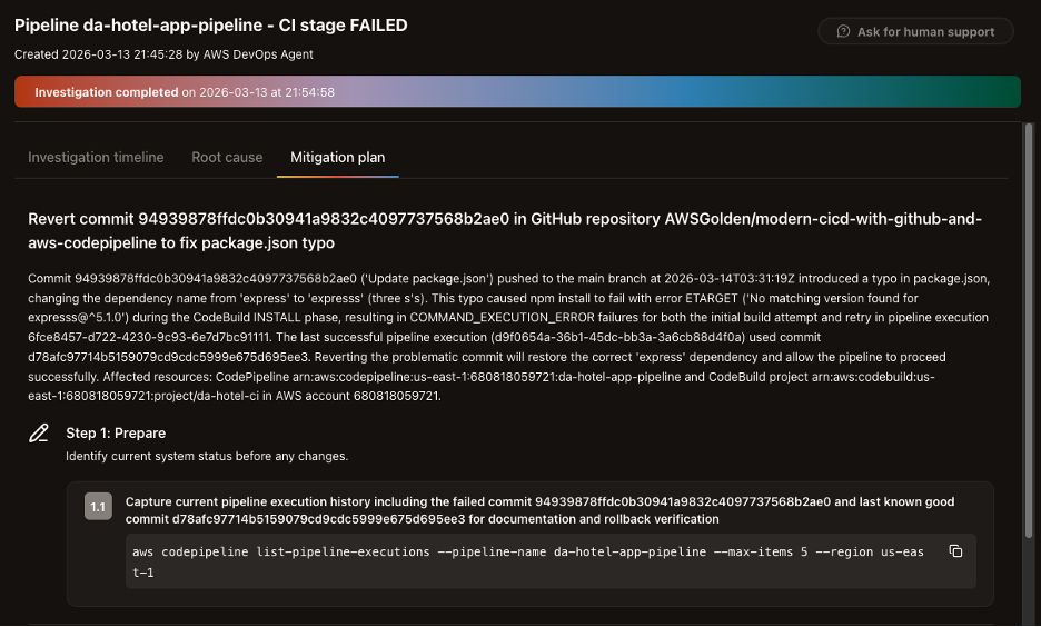
Automated incident remediation – turning investigation findings into deployed fixes without manual toil – is the next frontier for operations teams running distributed workloads on AWS. Today, when an incident fires at 2 AM, the on-call engineer must correlate telemetry across Amazon CloudWatch, deployment pipelines, and application logs, then manually write and deploy a fix – a process that routinely takes hours. AWS DevOps Agent addresses the first half by autonomously investigating incidents, identifying root causes, and generating mitigation plans in minutes. During preview, customers and partners reported up to 75% lower MTTR, 80% faster investigations, and 94% root cause accuracy.
But investigation and mitigation recommendations are only half the story. Someone still has to read the findings, write the fix, test it, and deploy it. What if that second half could be automated too?
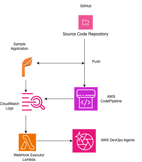
In a previous post, Leverage Agentic AI for Autonomous Incident Response with AWS DevOps Agent, we demonstrated how to configure AWS DevOps Agent to monitor your applications, trigger autonomous investigations, and follow best practices for production deployments. We also published this code sample which demonstrates how investigations could be wired to be triggered automatically when a Amazon CloudWatch alarm is raised. These two articles now allow you to trigger AWS DevOps Agent investigation on a Amazon CloudWatch alarm and produce a mitigation plan.
In this post, we demonstrate how to integrate AWS DevOps Agent mitigation plan output with Kiro CLI – running in headless mode on AWS CodeBuild – to close the remediation loop end-to-end. When AWS DevOps Agent completes a mitigation analysis, an event-driven pipeline automatically routes the findings to Kiro CLI, which applies the fix to your codebase, creates a pull request for human review, and triggers deployment upon approval. The result: L1/L2 incidents go from detection to deployed fix with minimal manual intervention – the only human touchpoint is the pull request approval.
We walk through the complete solution using a sample CloudFormation application, including the infrastructure code, anomaly generation scripts, event routing, and the Kiro CLI steering configuration that makes it all work. All source code is available in the accompanying aws-samples repository.
Solution Overview
Consider a typical web application running on AWS — a frontend behind an Application Load Balancer, backend compute on Amazon EC2, and an Amazon RDS database, with source code and CloudFormation templates in AWS CodeCommit. When something goes wrong in this environment, the solution chains two AWS frontier agents —AWS DevOps Agent for autonomous investigation and mitigation, and Kiro CLI for automated code remediation — through a fully serverless event-driven bridge to take the application from incident to deployed fix.
Fig 1 – Solution architecture
How it works
An incident occurs – Your application experiences an issue – high CPU utilization, elevated error rates, slow response times. Amazon CloudWatch alarms fire.
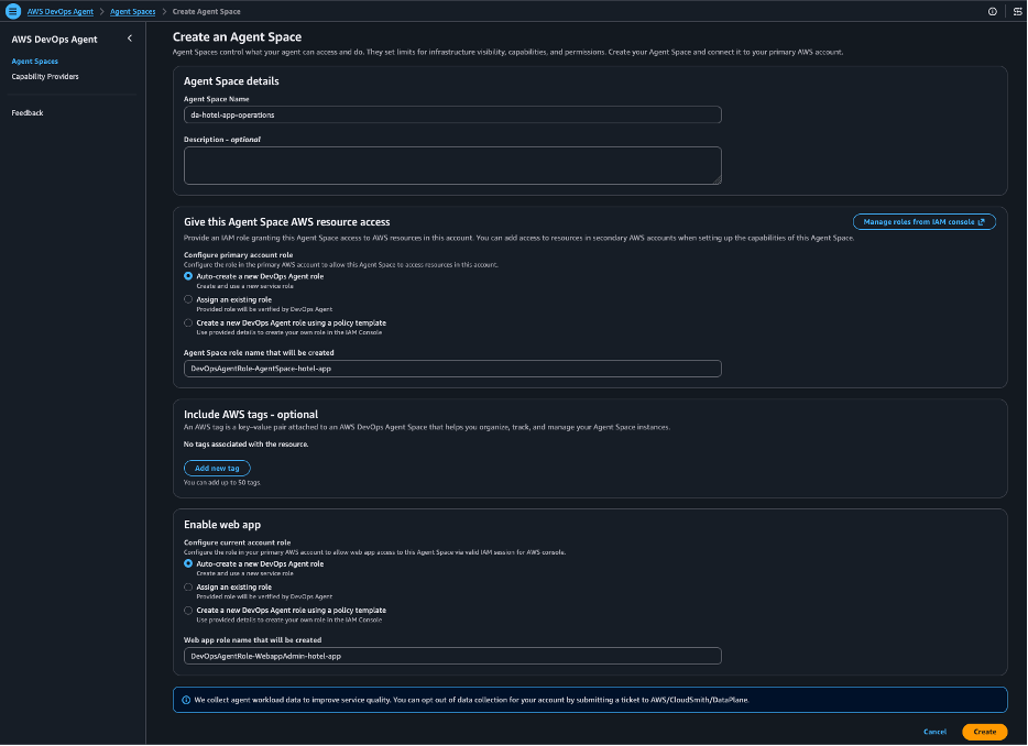
DevOps Agent investigates – AWS DevOps Agent, which has your application onboarded into an Agent Space, autonomously correlates metrics, logs, and deployment history to identify root cause and generate a mitigation plan.
EventBridge routes the signal – An Amazon EventBridge rule captures Mitigation Completed events (source: aws.aidevops) and invokes a AWS Lambda function.
Lambda extracts and queues – The AWS Lambda function calls the AWS DevOps Agent API to retrieve the mitigation summary and execution plan, then publishes the payload to Amazon SQS queue.
CodeBuild runs Kiro CLI – When a message arrives in the Amazon SQS queue, a AWS Lambda function with an SQS event source mapping triggers a AWS CodeBuild execution, passing the message content as an environment variable. AWS CodeBuild runs Kiro CLI in headless mode (–no-interactive –trust-tools=read,write,grep,shell), using the mitigation payload as a remediation prompt.
Kiro CLI applies the fix – Guided by a steering file that describes the repository structure and remediation conventions, Kiro CLI modifies the CloudFormation template or application code, commits to a feature branch, and creates a pull request.
Human approves, pipeline deploys – A developer reviews the pull request. Upon approval and merge, the associated deployment pipeline gets triggered to execute the change.
The sample repository pushed to your account’s AWS CodeCommit repository
Once completed, follow along the Readme file to setup the components which allow you to implement and execute the above architecture. The sections below provide an explanation of the components that have been built to support the architecture.
Capturing mitigation events
AWS DevOps Agent publishes lifecycle events to the Amazon EventBridge default event bus whenever an investigation or mitigation changes state. Each event uses the source aws.aidevops and a detail-type that identifies the specific like Mitigation Completed, Investigation Completed, or Mitigation Failed. The post focuses on a single signal: the moment a mitigation finishes successfully.
EventBridge rule and Lambda extraction
An Amazon EventBridge rule matching the Mitigation Completed detail-type invokes a AWS Lambda function. The event payload contains metadata (agent_space_id, task_id, and execution_id) which allows the AWS Lambda function to call the AWS DevOps Agent and extracts two key objects: the mitigation summary (what action to take and why) and the execution plan (step-by-step instructions). It publishes this structured payload to an Amazon SQS queue for downstream processing.
Headless remediation with Kiro CLI
With mitigation payloads landing in the Amazon SQS queue, we need a compute environment that can check out the application and infrastructure repository, run Kiro CLI agent against the codebase, and push changes back. AWS CodeBuild is a natural fit — it provides on-demand compute, integrates natively with AWS CodeCommit and requires no persistent infrastructure.
Kiro CLI 2.0 introduced headless mode, which allows it to run programmatically in deployment pipelines without an interactive terminal. You authenticate with an API key (stored in AWS Secrets Manager), pass a prompt, and Kiro CLI executes end-to-end — same tools, same agents, same capabilities as the interactive experience.
How CodeBuild orchestrates the fix
When a message arrives in the Amazon SQS queue, a trigger AWS Lambda function starts a AWS CodeBuild execution, passing the Amazon SQS message body as an environment variable. The AWS CodeBuild buildspec follows a straightforward sequence:
Install : Installs Kiro CLI and configures the environment. The KIRO_API_KEY is pulled automatically from AWS Secrets Manager ,never hardcoded.
Generate prompt: A Python script converts the structured mitigation payload into a natural-language remediation prompt. It inspects the content to classify whether the change targets infrastructure (or application code, then generates a focused prompt with the action, reasoning, and specific instructions.
Create feature branch : Checks out a new branch named after the agent space and execution IDs for traceability.
Run Kiro CLI : Invokes Kiro CLI chat –no-interactive –trust-tools=read,write,grep,shell with the generated prompt. The –trust-tools flag auto-approves specific tool categories following least-privilege, since there is no human to confirm.
Validate and commit : Guardrails check the changes: file count limits, protected file detection, Python syntax validation (py_compile), and YAML linting. If all checks pass, the changes are committed and pushed.
Create pull request : Creates an AWS CodeCommit pull request with the mitigation action as the title and the AWS DevOps Agent reasoning in the description.
The steering file
What makes Kiro CLI effective at remediation – rather than just generating generic code – is the steering file. Steering gives Kiro persistent knowledge about your project: repository structure, coding conventions, and decision frameworks.
For this solution, the steering file serves as the guardrails for automated remediation. It defines:
Repository structure – Maps each directory to its purpose.
Decision framework – Rules for classifying changes as infrastructure vs. application.
Scope constraints – Maximum 3 files per remediation, no new files, no new dependencies, no deletions.
Protected files – The buildspec, infrastructure pipeline templates, bridge code, and steering files themselves are explicitly off-limits.
Fail-safe – If the prompt is ambiguous or Kiro cannot determine what to change, it makes no changes rather than guessing.
This steering file is committed to the repository, so every AWS CodeBuild execution picks it up automatically. It ensures Kiro CLI makes targeted, predictable changes rather than broad refactors.
From pull request to deployment
At this point, the automated pipeline has done its work – Kiro CLI has analyzed the mitigation plan, modified the appropriate files, and created a pull request on a feature branch. The pull request description includes what was changed, why (directly from the AWS DevOps Agent’s reasoning), and the agent space and execution IDs for full traceability back to the original incident.
This is where the human-in-the-loop gate comes in. A developer reviews the pull request -verifying that the change is correct, scoped appropriately, and safe to deploy. This approval step is deliberate: while we trust the agents to investigate, analyze, and propose fixes, a human makes the final deployment decision.
Once the pull request is approved and merged into the main branch, the deployment pipelines implement the approved changes in the target environment.
The entire cycle – from CloudWatch alarm to deployed fix – completes in minutes rather than hours, with the only manual step being the pull request review. For organizations handling high volumes of L1/L2 incidents, this translates directly into reduced operational toil and faster recovery.
Cleanup
To avoid ongoing charges, remove the resources created during this walkthrough. Refer to the Readme for the complete teardown sequence.
Conclusion
In this post, we demonstrated how to integrate AWS DevOps Agent mitigation outputs with [1] Kiro CLI to build a closed-loop incident remediation pipeline. By connecting these two frontiers agents’ operations teams can go from incident detection to deployed fix with a single human touchpoint: the pull request approval.
This approach delivers measurable impact for enterprise operations:
Reduced MTTR – L1/L2 incidents that previously required hours of manual investigation and remediation can now resolve in minutes.
Improved operator productivity – Engineers shift from reactive firefighting to reviewing and approving targeted, AI-generated fixes.
Consistent remediation – Steering files codify your team’s conventions and decision frameworks, ensuring every automated fix follows the same standards regardless of when or how often incidents occur.
Ready to get started? Clone the aws-samples repository for the complete implementation, visit the AWS DevOps Agent documentation to configure your first Agent Space, and explore the Kiro CLI documentation to learn more about steering-file-driven code generation. Have questions or want to share how you’ve adapted this pattern? Leave a comment below or open an issue in the repository
A single cold start can push your Java Lambda function’s response time from milliseconds to seconds, enough to violate your p99 SLA, timeout a downstream service, and page your on-call. The Java Virtual Machine (JVM) performs best in long-running processes. Its Just-In-Time (JIT) compiler progressively optimizes code over thousands of invocations. Standard serverless execution environments recycle before the JVM reaches peak performance. This creates a tradeoff for latency-sensitive applications between cold-start penalties and runtime optimizations. For production services with p99 service level agreement (SLA) requirements, a single 14-second cold start spike can violate response time guarantees. It triggers downstream timeouts and degrades customer experience.
AWS Lambda Managed Instances changes this equation. As a capability of AWS Lambda, Managed Instances runs your functions on managed Amazon Elastic Compute Cloud (Amazon EC2) instances in your account and maintains JVM persistence across invocations. Connection pools, class hierarchies, and heap state persist across thousands of requests. This allows the JIT C2 compiler to complete optimizations like method inlining, escape analysis, and loop unrolling. The result: 18 to 30% better median latency and 3 to 30x better tail latency compared to Standard Lambda, as the benchmarks in this post demonstrate.
This post benchmarks four Java deployment modes across three workload types using 240,000 requests. The modes compared are Standard Lambda, AWS Lambda SnapStart, GraalVM Native Image, and Lambda Managed Instances. The workload types are CPU-bound, I/O + computation, and I/O-bound. This post presents benchmark results demonstrating Managed Instances delivering 30% better median latency and removing multi-second cold-start spikes on CPU-bound work after JIT warmup. It explains why these gains occur, maps each deployment mode to specific traffic patterns and cold-start tolerance requirements, and provides a decision framework for selecting the right approach for your workload.
Benchmarking setup
The benchmark runs all four deployment modes with identical Spring Boot 4.0.6 applications on Java 25 and AWS SDK v2. This configuration verifies fair comparison across modes. We tested three workloads: UC1 (PDF generation, CPU-bound), UC2 (data aggregation, I/O + computation), and UC3 (API orchestration, I/O-bound). The benchmark sends 240,000 requests using Artillery load testing at 33 RPS. Standard Lambda, SnapStart, and Native Lambda use 1024 MB (1 vCPU). Managed Instances uses c7i.xlarge instances with 2048 MB memory. Concurrency is tuned per workload (UC1=3, UC2=5, UC3=10) based on load testing to avoid thread contention. The benchmark measures p50, p99, and maximum latency across 10 runs of 2,000 requests each, with 5-minute cool-down between runs. The benchmark tracks JIT compilation metrics via Amazon CloudWatch Embedded Metrics Format. You can validate these results against Amazon API Gateway access logs, which confirm a <0.1% error rate. The GitHub repository contains complete source code, AWS Serverless Application Model (AWS SAM) templates, load scripts, and raw data. Performance claims in this post reference data from this benchmark methodology.
Figure 1 presents the architecture for all four deployment modes running in parallel against shared backend services.
To reproduce these benchmarks or deploy the sample applications, refer to the GitHub repository. The repository contains complete SAM templates, Artillery load configurations, deployment instructions, and cleanup commands. This post focuses on benchmark results and analysis. The benchmark used the following tools and services:
Managed Instances removes the extreme tail spikes characteristic of cold starts. Managed Instances delivers 27x faster maximum latency on CPU-bound workloads (UC1: 489 ms vs. 13,270 ms Standard). Mixed I/O + compute workloads see a 3x improvement (UC2: 3,644 ms vs. 11,174 ms Standard). I/O-bound workloads improve 30x (UC3: 309 ms vs. 9,237 ms Standard). We measured all results using the methodology described in Benchmarking setup.
The Standard Lambda 13-second maximum on UC1 represents a full cold start. That cold start includes JVM boot, Spring context initialization, Amazon DynamoDB client setup, and the first PDF render. SnapStart reduces this to under 3 seconds by restoring from a Firecracker microVM snapshot. However, the restore process plus re-initialization of resources that cannot be checkpointed (network connections, random number generators) still adds latency. GraalVM Native starts in under 2 seconds because the ahead-of-time (AOT) compiled binary skips JVM boot entirely. The Managed Instances maximum of 487 ms is not a cold start; it’s the slowest warm request across 20,000 invocations. For production SLAs, a 14-second cold start spike on Standard Lambda violates most requirements, while Managed Instances removes that spike entirely.
Observing median latency (p50)
Lambda Managed Instances delivered the lowest median latency across all three workloads. Results demonstrate 30% faster median latency on CPU-bound workloads (UC1: 97 ms vs. 139 ms Standard). Mixed I/O + compute achieves a 19% improvement (UC2: 184 ms vs. 228 ms Standard). I/O-bound workloads improve 18% (UC3: 76 ms vs. 93 ms Standard).
The improvement scales with CPU intensity because the JIT C2 compiler on persistent Managed Instances optimizes hot code paths that short-lived serverless environments never reach. On CPU-bound workloads (UC1), the JIT compiler has more opportunity to optimize tight loops in PDF rendering. On I/O-bound workloads (UC3), network latency to Amazon DynamoDB, Amazon SQS, and Amazon SNS dominates the request duration, so JIT optimization provides smaller gains.
Observing tail latency (p99)
Managed Instances showed even larger improvements at the tail of the latency distribution. The p99 improves 36% on CPU-bound workloads (UC1: 225 ms vs. 353 ms Standard). Mixed I/O + compute achieves a 41% improvement (UC2: 1,883 ms vs. 3,201 ms Standard). I/O-bound workloads improve 27% (UC3: 193 ms vs. 265 ms Standard).
UC2 showed the largest p99 improvement (41%) because data aggregation combines DynamoDB queries, returning hundreds of records with in-memory statistical computation and Amazon S3 uploads. Standard Lambda environments that haven’t fully warmed their JIT produce significantly slower responses at the tail. The persistent JIT optimization (-Xms512m -Xmx1408m) with G1 garbage collection (GC) and explicit heap sizing on Managed Instances both contribute to tighter tail latency distribution. For services with SLAs on p99 response time, this reliability improvement matters more than median performance. For workloads with significant heap pressure, tuning -XX:MaxGCPauseMillis and monitoring GC logs can further tighten tail latency.
Why Lambda Managed Instances is faster: JIT compilation
The JVM’s Just-In-Time compiler works in tiers. The C1 compiler performs initial compilation quickly with basic optimizations. The C2 compiler profiles execution over hundreds of invocations and then applies aggressive optimizations: method inlining (eliminating function call overhead), escape analysis (allocating objects on the stack instead of the heap), loop unrolling (reducing branch overhead), and vectorization (processing multiple data elements in a single CPU instruction).
The following table presents JIT warmup progression using java.lang.management.
CompilationMXBean emitted through Amazon CloudWatch Embedded Metrics Format. We collected this data from a 1,500-request sustained load test on UC1 (PDF generation):
Phase
Invocation
Avg Latency
What’s Happening
First requests (application init)
1
~2,400ms
JVM boot, spring context creation, SDK client setup
Early requests (C1 compiled)
2-100
~145ms
C1 compiler active. App is functional, but not optimized
Steady state (C2 optimized)
1000+
~38ms
C2 optimizations completed
The first invocation includes one-time application start costs: class loading, Spring context initialization, and DynamoDB client construction. These costs are unrelated to JIT compilation and occur on any deployment mode.
Once C1 compilation stabilizes during early invocations, latency reaches approximately 145ms. This is the baseline compiled performance. Over the next several hundred invocations, the C2 compiler profiles hot code paths and applies optimizations. By invocation 1,000, latency drops to 38ms. This represents a 3.8x improvement from JIT optimization alone.
Standard Lambda environments typically recycle before C2 completes its optimization passes. On Managed Instances, concurrent requests share the same JVM. This accelerates JIT profiling: three concurrent requests generate three times the method invocation data for the C2 compiler to optimize. The C2 compiler profiles execution patterns across all concurrent requests. It identifies hot code paths faster and applies optimizations sooner than single-concurrency environments.
What this means: CPU-bound workloads see the largest gains (30% faster median latency on UC1) because the JIT compiler has more opportunity to optimize tight loops and method calls. I/O-bound workloads see smaller gains (18% faster on UC3) because network latency to DynamoDB, SQS, and SNS dominates request duration. The JIT compiler still optimizes your code, but the network time remains constant across all deployment modes.
Choosing the right mode
No single mode wins in every scenario. The right choice depends on your traffic pattern, cold-start tolerance, team expertise, and operational complexity budget.
Lambda Managed Instances is ideal for steady-state traffic patterns above 5 requests per second with low cold-start tolerance (p99 SLA under 500 ms). Best for workloads with predictable, sustained traffic that need low latency with zero cold starts. Managed Instances excels at CPU-bound workloads where JIT optimization compounds.
SnapStart works well for variable traffic patterns where cold-start reduction matters. Choose this as the default for Java Lambda functions. SnapStart reduces cold starts with minimal code changes (add CRaC priming). You have no additional infrastructure to manage. Works with the existing Lambda scaling model.
GraalVM Native Image works well for bursty traffic patterns with strict cold-start tolerance (sub-second cold starts required). Ideal if your team can invest in AOT compatibility (reflection configuration, build pipeline). This mode offers a smaller memory footprint. Requires testing for SDK compatibility.
Standard Lambda is the baseline for low-traffic or burst workloads where cold starts of 6-14 seconds are acceptable. Works well when invocation frequency is low enough that per-request billing is cheaper than fixed instance costs, or when operational simplicity is the top priority.
For example, if you run a Spring Boot API handling 100 requests per second with a 400 ms p99 SLA, Lambda Managed Instances reduces your p99 from 353 ms (cutting it close) to 225 ms (comfortable margin) and removes the multi-second cold start spikes that violate your SLA entirely.
Dimension
Standard
SnapStart
Native
Managed Instances
Cold start
6-14 s
2-7 s
800 ms – 2 s
None
Warm p50 (CPU-bound)
139 ms
127 ms
107 ms
97 ms
Tail latency
Worst
Better
Good
Fastest
Error rate
Low
Low
Higher (SDK compat)
Low
Operational complexity
Lowest
Low
High (build pipeline)
Medium (VPC, sizing)
Burst scaling
Fastest
Fastest
Fastest
Slower (capacity provider)
Migration effort
None
Low (add CRaC priming)
High (AOT compat, reflection configuration)
Medium (capacity provider, VPC, thread safety)
Memory efficiency
Good
Good
Lowest
(125-154 MB)
Fixed per instance
Lambda Managed Instances supports Graviton4 (arm64) instances, which offer approximately 20% better price-performance based on AWS published Graviton4 benchmarks. These benchmarks use x86_64 for consistency across all four modes (GraalVM native cross-compilation to arm64 adds complexity). The arm64 parallelization characteristics could shift the performance curves for longer-lived deployment modes like Managed Instances in ways worth exploring in a future post.
Cost considerations
Lambda Managed Instances uses instance-based pricing rather than per-invocation billing. For steady-state workloads above approximately 9 requests per second, the fixed instance cost is lower than equivalent Standard Lambda GB-second charges. You can use the official pricing calculator to compare Managed Instances and standard Lambda costs.
Try it with your runtime version
These benchmarks use Java 25 with Spring Boot 4.0.6. The GitHub repository also includes configurations for Java 21 with Spring Boot 3.x. The repository README walks you through deployment, load testing, and collecting your own metrics.
Conclusion
This post demonstrates how Lambda Managed Instances solves a fundamental Java-on-serverless mismatch. The JVM’s JIT compiler needs time to optimize hot code paths. Standard Lambda recycles environments before the JVM reaches peak optimization. Managed Instances keeps the JVM alive across invocations, allowing the C2 compiler to reach peak optimization. The benchmarks show the impact. In these benchmarks, Managed Instances delivered 18 to 30% faster p50 latency than Standard Lambda. Tail latency improved 27 to 41% at p99. Maximum response times dropped 3 to 30x on CPU-bound workloads. The 3.8x improvement from JIT optimization alone shows what’s possible when the runtime has time to complete its work.
For more information, refer to the Lambda Managed Instances documentation. The GitHub repository contains the complete benchmark code, SAM templates, and deployment instructions. Share your results in the comments and let the community know how Managed Instances performs on your workloads. To delete all benchmark resources and avoid ongoing charges, run the cleanup commands documented in the GitHub repository README.
This essay was written with Nathan E. Sanders, and originally appeared in The Guardian.
Opposition to AI data centers has emerged as a primary theme in US politics, one that—surprisingly—doesn’t fallalong party lines. We applaud people coming together for constructive debate on any issue, and agree that communities need to evaluate whether any economic benefits these data centers bring is worth their costs. Still, we worry that a focus on data centers obscures the larger impacts of AI on people’s lives: the concentration of power of AI companies, and their widespread political and financial influence.
Local data center opposition is grounded in legitimate concerns about misallocation of land resources when housing is at a premium, pressures on already higher energy prices, and localized environmental impact. Unlike other resource-consuming and polluting industrial facilities, data centers produce very few jobs. The fact that US opposition to data centers seems to be most fierce among lower-income communities reflects righteous indignation with an inequitable bargain, where tech companies and developers profit from exploiting local resources but offer little in return. On a global scale, their carbon footprint could grow unsustainably if usage accelerates. And all this is in aid of a technology that many fear will propagate misinformation, take their jobs, or even cause existential risks for humanity.
For some, data center opposition may feel like the only tangible mechanism for registering their concern, disapproval, or even anger about AI. The problem is that this may be exactly what the AI companies are banking on. They can overcome the protest when it matters to them, and live with a significant fraction of proposals being defeated. More importantly, focusing political opponents on the data center issue obscures the bigger prize they’re after.
While there is a staggering three-quarters of a trillion dollars being spent on data center infrastructure by US companies this year alone, this investment should be taken in perspective. The market for enterprise software, for example, is about twice this size. And it’s small compared with what these companies actually want.
AI companies have their eyes set on capturing all the value created by entire industries. The technology has arguably already conquered customer service and consumer sales. But on the horizon are bigger targets, such as enterprise software development, creative design, management and even legal services. In AI companies and their allies’ vision of the future, AI replaces teachers and doctors. The companies would rather spend time fighting resistance to how fast they are building computing infrastructure than dealing with issues of how their products should be used in those fields, or how those fields should be protected from their products.
And while data center opposition campaigns have been successful in building widespread appeal, their effectiveness in the US is mixed. They seem to be most successful when organizing against speculative, early-stage data center proposals that have a relatively low likelihood to ever see fruition. Meanwhile, advanced-stage, well-capitalized data center projects have proven to have the resources to overcome local opposition. An OpenAI- and Oracle-backed facility in Saline township, Michigan, is breaking ground on construction even after local officials voted to reject it. The developers sued the town of 3,000 and forced a settlement that involved their project going forward. Meanwhile, the Trump administration, a vigorous ally of corporate AI, has signaled its willingness to advance AI infrastructure development by overriding state objections and even using federal lands.
Also consider that rampant data center development may be a momentary spike rather than a longstanding concern. Demand for the centralized computing that data centers provide may well decline over time. The leading Chinese labs, such as Z.ai, are innovating in technical mechanisms to make frontier-class models smaller and cheaper to run. AI power users have become adept at miniaturizing open weight models, ones published free for anyone to download and use, to run locally on their own computers. Apple and Googleboth support infrastructure stacks for running AI models directly on mobile phones. It could be that the current mania for data centers will look like the fiber optic cable bubble from the early 2000s, as demand shifts to smaller models and AI usage on people’s own devices.
For those concerned primarily with affordability and environmental protection, singling out data center construction is misplaced. Energy rates and inflation today seem to be most visibly affected by the US-Iran war. The US is disinvesting in long-term energy security by ceding the renewable energy industry to China and actively cancelling climate commitments. Consider that 10% of global carbon emissions stem from heating buildings, which dwarfs energy use by AI and could be cut fivefold by using heat pumps powered by renewable energy. With respect to housing affordability, federal housing subsidies have changed little over three decades, in inflation-adjusted terms, even as housing costs have spiked and homeowners have enjoyed robust tax incentives.
As for AI itself, the concentration of power and wealth in these tech companies is the greatest existential risk facing society today. This means we must limit corporate power, especially corporations’ ability to exploit the public and manipulate our political system.
Opposing data centers should be just a starting point. We can advocate for states to regulate AI, to reject irresponsible uses of the technology, and shape corporate behavior. We can fight for AI computation to be taxed, so that the public can capture some of the profit of AI use while also forcing AI companies to internalize more of the energy and environmental consequences associated with its use. And we all can join the global movement for Public AI, an alternative ecosystem for AI that is developed under public control with an incentive structure to create public benefit rather than private profit.
The US midterm elections present ample opportunity for those seeking to control the AI political agenda. In the recent New York congressional Democratic primary, PACs linked to the dueling AI companies Anthropic and OpenAI spent millions of dollars lobbying for or against “AI safety“, the idea that we must urgently monitor and prevent people from using AI to cause catastrophic harms. We’re already seeing a similar dynamic play out in races in Massachusetts and other states.
Why would Anthropic and OpenAI—bitter industry rivals but fundamentally on the same side politically—support opposing viewpoints? Because they both ultimately profit from the mystique: the idea that their products are so powerful that controlling those products is the world’s most important challenge. Here’s the typical read on the dynamic. To one side (backed by OpenAI affiliates), “safety” comes from the appearance of US industry dominating AI innovation, under the slow-moving control of federal lawmakers (and without pesky state regulators in the way). To the other side (backed by Anthropic), “safety” means a heavier regulatory framework that plays to Anthropic’s posturing as the ethics- and compliance-focused AI vendor. In both cases, it’s more marketing than principled concern about safety.
Political organizers should call out and reject the AI companies’ framing of the debate, and reorient campaign agendas around populist resistance to corporate concentration of wealth and power. When AI companies pump millions into legislative races, the result should not be hyperbolic discussion of AI superintelligence. And when a plot of land in a small town is pitched as a data center site, the debate should be about more than the local costs and benefits. It should include out-of-control money in politics, and Citizens United-proof solutions to limit corporate influence like public financing and state regulation.
We all have a vested interest in what’s on the policy agenda, and what the outcomes are. Today, the greatest risk AI poses to society is the exacerbation of inequality and the concentration of wealth. The real problem is trillion-dollar AI companies and their trillionaire oligarchs cozying up to political power in Washington and governments worldwide, and using their money to enact their agenda over the popular will of the people. This is the issue we’d like to see put front and center, and it requires solutions much more extensive than slowing data center development.
We recently announced the launch of AWS Lambda MicroVMs, a new serverless compute primitive that provides VM-level isolation, near-instant startup performance, and state retention. You can now give each user or job their own execution environment to securely run just-in-time code – either user or AI generated – without managing virtualization infrastructure or choosing between isolation, speed, and state retention. Lambda MicroVMs are powered by Firecracker virtualization, the technology underpinning AWS Lambda. You can use Lambda MicroVMs to build data analytics applications, AI sandboxes, vulnerability scanners, and interactive development environments.
Evolution of serverless compute
When we launched AWS Lambda in 2014, the premise was simple: give developers a way to run code without thinking about servers. Upload a handler, configure a trigger, and let the service handle infrastructure provisioning, scaling, patching, and availability. Over the past decade, Lambda has grown to process tens of trillions of requests each month for over 1.5 million customers. Under the hood, those invocations run inside a Lambda-managed Firecracker microVM – a lightweight virtual machine that combines hardware-level virtualization and near-instant startup speed. With Lambda SnapStart, we used Firecracker’s snapshotting capabilities to accelerate startup times by resuming execution environments from pre-initialized snapshots (carrying memory and disk state) rather than cold-booting them.
Today, a growing class of applications need to run code supplied by users or AI agents just-in-time – and need Firecracker’s core capabilities directly: hardware isolation, near-instant startup, and state retention over extended periods. Achieving this today often requires building custom infrastructure that diverts teams from core application development. We’ve been hearing this theme from customers across use cases and industry verticals:
Interactive code environments like browser-based IDEs, notebooks, and vibe-coding platforms need to deploy and execute user-generated code in per-user environments that start within seconds and retain state – like installed packages, generated files, and running processes – across interactions.
Data analytics platforms run user-supplied or LLM-generated queries and notebooks in isolated environments that retain large working sets over long durations – such as an 8-hour workday – with the ability to resume quickly after periods of inactivity.
AI coding assistants and agents run LLM-generated code iteratively, while retaining context between iterations, and rapidly launching and shutting down environments to evaluate alternative code paths, such as for reinforcement learning.
IT security scanners execute vulnerability assessments in compute environments that are strongly isolated from one another, can scale to handle bursts of concurrent scan requests, and support elevated operating system privileges.
CI/CD platforms need ephemeral, isolated build and test environments that start quickly and can be discarded after each run.
Introducing Lambda MicroVMs
Now, with AWS Lambda MicroVMs, developers can directly use the isolation, speed, and state snapshotting of Firecracker MicroVM as a primitive, while keeping the serverless simplicity of AWS Lambda. Lambda MicroVMs provide these key capabilities.
Snapshot-based, near-instant startup: To optimize startup speed, MicroVMs are launched from MicroVM images, which are pre-initialized Firecracker snapshots of your application’s memory and disk state. When you create a MicroVM image, the service executes your Dockerfile, initializes your application, and snapshots the MicroVM. Lambda starts MicroVMs from this snapshot with your dependencies loaded.
Direct HTTPS connectivity: Each MicroVM exposes a dedicated HTTPS endpoint for inbound connectivity to individual ports. You can connect to applications running within your MicroVM using standard HTTPS clients, WebSocket connections, or gRPC – exactly as you would with a container or VM.
Lifecycle control with state retention: Lambda MicroVMs allow you to control the lifecycle of each execution environment, enabling you to support interactions that last a few minutes to sessions that span 8 hours.
Vertical and horizontal scaling: Each MicroVM starts with a configurable baseline — 2 GB memory and 1 vCPU by default (up to 8 GB and 4 vCPUs), with CPU allocated in a 2:1 ratio to memory. From that baseline, MicroVMs scale vertically by up to 4x automatically, meeting peak resource demands for each user or session without any action on your part. MicroVMs also scale horizontally — you can launch several hundred within a minute during traffic spikes. For details on service limits, refer to Lambda service quotas.
Internet and VPC access: By default, Lambda MicroVMs support outbound connectivity to the public internet without additional configuration. For private VPC connectivity to resources such as databases or internal APIs, you can use a Lambda Network Connector (LNC). LNC is a new Lambda resource that provides managed, configurable network connectivity between your MicroVMs and your private VPC.
Building with Lambda MicroVMs
Lambda MicroVMs introduces two core resource types: a MicroVM image – a versioned artifact containing your runtime environment and application code, and MicroVMs – individual instances launched on demand from a MicroVM image.
Let’s make this concrete with an example. You are a cloud architect building a data analytics application which under the hood, manages compute environments to generate insights for data analysts within your organization. Analysts load multi-gigabyte datasets and generate visualizations in sessions that last hours with idle gaps when they switch to other tasks. When analysts return, they expect to pick up exactly where they left off. Here’s how you can use MicroVMs for this workload:
Step 1: Define your environment
Write a Dockerfile that installs your data science stack. This runs once at MicroVM image build time – every analyst’s MicroVM starts with these dependencies already loaded. This Dockerfile builds a notebook server that accepts code execution requests, runs them in-process (so state accumulates across requests), and returns results. Your customer-facing UI calls this notebook server for each analyst.
FROM public.ecr.aws/lambda/microvms:al2023-minimal
# Install Python 3.12 and pip
RUN dnf install -y python3.12 python3.12-pip && dnf clean all
RUN pip3.12 install --no-cache-dir \
pandas numpy scipy scikit-learn matplotlib seaborn \
fastapi uvicorn boto3 pyarrow
COPY notebook_server.py /app/notebook_server.py
WORKDIR /app
EXPOSE 8080
CMD ["python3.12", "notebook_server.py"]
Next, package and upload your application artifacts and Dockerfile to S3.
When you create a MicroVM image, Lambda executes your Dockerfile, starts your application, and takes a Firecracker snapshot of the fully initialized environment with the libraries imported, and notebook server listening. Every MicroVM launched from this image skips this initialization step, and provides near-instant startup.
Step 2: Launch a MicroVM when an analyst starts their session
Once your MicroVM image is ready, you can start a new MicroVM for each analyst session. The idle policy encodes your business logic: auto-suspend after 5 minutes of inactivity, retain the suspended state for up to 8 hours (covers a full workday), and auto-resume when the analyst’s next request arrives. Within seconds, the analyst has a dedicated environment with their own filesystem, and a dedicated HTTPS endpoint.
aws lambda-microvms run-microvm \
--image-identifier arn:aws:lambda:us-east-1:123456789012:microvm-image:analytics-notebook \
--image-version 1.0 \
--idle-policy '{"maxIdleDurationSeconds":300,"suspendedDurationSeconds":28800,"autoResumeEnabled":true}' \
--maximum-duration-in-seconds 28800 \
--execution-role-arn arn:aws:iam::123456789012:role/notebook-exec-role \
--region us-east-1
# MicroVM endpoint url is returned by the run-microvm API call
ENDPOINT="https://a1b2c3d4-e5f6-7890-abcd-1234567890ef.lambda-microvm.us-east-1.on.aws"
When a data analyst submits a query, it is submitted as an HTTPS request to their assigned MicroVM. You can test this using curl on the MicroVM endpoint.
Notice that you can separate the build-time IAM role from the execution-time IAM role for finer-grained control over each tenant’s permissions.
Step 3: Suspend and resume during idle periods
After 5 minutes of inactivity, the MicroVM is automatically suspended based on the configured idle policy. When the MicroVM is suspended, its memory and disk state is preserved.
Two hours later, the analyst returns and sends the next query. The MicroVM auto-resumes within seconds. The memory and disk state are restored exactly as the analyst left them – no re-computation or re-loading required.
Analysts can also suspend and resume their MicroVMs directly using the APIs.
If your data lives in a private VPC, for example, Amazon Redshift clusters or RDS databases, you can use a Lambda Network Connector (LNC) to give your analysts MicroVMs access to this data. Create a network connector once:
To recap, with MicroVMs we build an image once, launch isolated MicroVMs per user or job, interact over HTTPS, suspend when idle, and terminate when done. This pattern applies broadly, across use cases. For instance, an IT security platform scanning customer repositories has similar requirements: an isolated environment per scan, the ability to run with elevated operating system privileges, and rapid horizontal scaling to hundreds of concurrent scans. Similarly, an AI coding assistant needs per-developer sandboxes that retain installed packages and generated files across iterative code-write-test cycles, with suspend/resume preserving context when developers switch tasks. In each case, the workflow is the same.
Building MicroVMs with Agent Toolkit for AWS
In the previous section, we demonstrated Lambda MicroVMs core API operations. You can also use your preferred Agentic development tools to start developing with Lambda MicroVMs. Simply install the AWS Lambda MicroVMs skill from the Lambda MicroVMs console, or use the Agent Toolkit for AWS.
To get started in the AWS Lambda console, choose the highlighted button to access the MicroVMs agent instructions as in Figure 1:
Figure 1: Access MicroVM agent instructions
Next, copy the agent installation instructions and paste it in your terminal to begin developing.
Figure 2: Copy agent instructions
The following screenshot demonstrates the skill in action in an AI coding assistant. Using the skill, the coding assistant agent generates a detailed plan to build the analytics notebook solution, executes the plan, and validates correct execution.
Figure 3 continued: Agent-driven development with MicroVMs
Lambda MicroVMs as sandboxes for Claude Managed Agents
You can also use AWS Lambda MicroVMs as a managed sandbox provider for Claude Managed Agents self-hosted sandboxes. This pattern keeps the orchestration within your Anthropic environment, which hosts the agent loop and Claude model, but moves tool execution into AWS Lambda MicroVMs, so the agent’s code, filesystem, and network egress never leave the infrastructure you control. You control the execution environment – what is installed, what network access is available, and what resources the agent can reach. For integration details, refer to the Lambda MicroVMs developer guide.
Snapshot compatibility considerations
Lambda MicroVMs are started from snapshots of pre-initialized memory and disk state. This has a few implications for how you build applications:
Uniqueness: Content generated and retained within a MicroVM image is shared across all MicroVMs started from that image. To maintain uniqueness for content such as unique IDs, secrets, or random seeds, generate these values after each MicroVM is started. If your application code uses OpenSSL, use the AWS-provided base container image from public.ecr.aws/lambda/microvms:al2023-minimal to build your MicroVM image.
Ephemeral credentials and network connections: Credentials and connections established during MicroVM image creation – or before a MicroVM is suspended – may expire or terminate by the time the MicroVM starts or resumes. Design your application to refresh these credentials and re-establish connections on startup. AWS SDK clients re-establish connections automatically in most cases.
Lambda MicroVMs provides lifecycle hooks that are executed when a MicroVM is started or resumed. Use these hooks to restore uniqueness and to re-establish network connections or ephemeral credentials. For more details, refer to the Working with snapshots section in the Lambda MicroVMs developer guide.
Pricing
Lambda MicroVMs pricing comprises compute, snapshots, and data transfer (at standard AWS rates, including data transferred to your VPC). You have two cost management levers: baseline-plus-consumption billing and idle-suspension. With baseline-plus-consumption billing, your bill tracks closer to your actual resource usage rather than peak resource usage. You configure your MicroVM’s baseline resource allocation to match your workload’s average resource utilization – not peak. During peak activity, your MicroVM can vertically scale up to 4x of the configured baseline automatically and resource usage above the baseline is only billed during active use. You configure the baseline by setting memory, and CPU is allocated in a 2:1 memory-to-CPU ratio – the default is 2GB / 1vCPU, with a corresponding peak of 8 GB / 4 vCPU. Supported baseline and peak values are shown in Figure 4.
Figure 4: Baseline and peak resource configuration
During extended idle periods, you can suspend your MicroVM to preserve memory and disk state at storage-only rates, resuming near-instantly when needed – no compute charges while suspended. For full pricing details, see AWS Lambda pricing.
Conclusion
Lambda MicroVMs extends the serverless compute model beyond invocation-based functions to long-running, stateful environments that execute code supplied by end users or AI. Development teams can focus on core application development while Lambda provides secure isolation and near-instant startup performance. Whether you’re building an AI coding assistant, an interactive development platform, an IT security platform, or a data analytics workload, the pattern is the same: define your environment in a Dockerfile, build a MicroVM Image once, launch isolated MicroVMs on demand, interact over HTTPS, and terminate when done.
In the near future, AI-powered surveillance systems will be able to track everything we do in public, and much of what we do in private. And if we do something wrong—shoplift, litter, jaywalk, you name it—the system will notice, retain it, tie it to your official government record, communicate that fact to you, and provide real-time alerts to any relevant authorities… and maybe also to the general public.
Think of these systems as automated speed cameras, but on steroids. Only they’ll enforce not just speed limits, but any other rule you can imagine. And you won’t receive a ticket weeks later by mail; you’ll be informed about and fined for your violation immediately.
These systems will combine powerful AI, public and private surveillance via real-time facial recognition technology and digital tracking, mass databases and highly personalized enforcement. If deployed at scale, they will have profound chilling effects not just on personal freedoms, but democracy and social progress itself.
China has been developing its surveillance infrastructure for years. The country has over 600 million surveillance cameras, increasingly powered by AI and facial recognition to enforce legal and social rules. Take the case of Lao Duan, a Chinese citizen blacklisted by the system after he lost his job and was unable to repay a series of loans. When he visited Beijing, the city’s AI surveillance system identified him by his face at a major intersection and displayed his face, name and citizen ID number on a large electronic billboard nearby with a message that he was an untrustworthy person. Similar systems are now being deployed across China and integrated with its infamous online monitoring, censorship and social credit systems.
AI surveillance is now being experimented with in North America, South America, Europe, Asia and Africa. According to a new report, the US Department of Homeland Security is rapidly increasing its use of AI-based surveillance, including facial recognition and the monitoring of social media accounts, to keep tabs on immigrants, dissidents, journalists, legal observers and protesters. While the systems are ostensibly used to maintain security and public safety, the real aim is often social control. Larry Ellison, CEO of Oracle—a powerful tech giant that works closely with the Trump administration—has said: “Citizens will be on their best behavior because we’re constantly recording and reporting.” The chilling effects are the point.
AI surveillance raises a range of public policy challenges: technical biases, unauditable systems, and inflexible automated law and social rule enforcement that can promote discrimination and undermine transparency, accountability and the rule of law. But we believe the most urgent and long-term impact will be its broader chilling effects.
In a new book, Chilling Effects: Repression, Conformity, and Power in the Digital Age, Jon Penney explains how surveillance, technology and power can be weaponized to influence behavior at scale. Surveillance, personalization, uncertainty and authority are all key mechanisms to increase the scale and impact of chilling effects. They cause people to self-censor their words and actions, to become more conformist and compliant and thus easier to manage and control. And the effects are additive: the more mechanisms employed, and the more powerful the form, the greater the chill.
Computerization has long allowed data collectors to track our locations, collect lists of whom we communicate with, and monitor our spending habits—unless we use cash. What’s new is an unprecedented fusion of each of these mechanisms, persistent and unrelenting. AI brings an analytical ability tospy on the contents of our communications, and to answer sophisticated questions about our whereabouts and activities: actions that previously required human analysts are now automated. The result will be a kind of supercharged societal level of chilling effects where fear, self-censorship and groupthink reign, and dissent, creativity and innovation become increasingly rare.
In this atmosphere of fear and conformity, risky ideas, social activism and self-reinvention—especially by disfavored groups and targeted populations—are also chilled. This will have long-term effects on social progress.
Consider the relatively recent societal normalization of same-sex relationships and the recreational use of marijuana. Over the decades, those ideas slowly progressed from being both immoral and illegal, to moral but still illegal, and finally to both moral and legal. But in order for any of that to happen, there had to be a counterculture that was able to experiment and eventually demonstrate to the world that morality could change over time. To the extent that AI surveillance chills this sort of experimentation in public or in private, social progress becomes impossible.
There are no real historical precursors to this; these technologies are too new. Even the most notorious and large-scale domestic surveillance program in US history, the FBI’s use of wiretapping, physical mail opening, informants and paper index cards to track alleged communists during the 1950s and 1960s, appears genuinely archaic in light of modern AI-enhanced surveillance. So does East Germany’s human-centric surveillance network during the cold war. Only science fiction, from the likes of George Orwell or Aldous Huxley, comes close. But even Big Brother’s “telescreen” feels decidedly mid-20th-century by comparison.
But we need not sit idly. Now that we recognize the danger of AI-enhanced mass surveillance, we can make the policy choices not to implement it. Bans on facial recognition and other forms of identification tech can slow development; robust new privacy and data protections can restrict data tracking and retention; AI regulations can curtail its most invasive uses; and structural reforms can help us scrutinize and break up powerful state/tech cartels that pave the way for technological excesses like AI surveillance.
The chill of AI-powered mass surveillance will suffocate the very foundations of healthy democratic societies. But we can still choose a different path.
This essay was written with Jon Penney, and originally appeared in The Guardian.
The collective thoughts of the interwebz
Manage Consent
To provide the best experiences, we use technologies like cookies to store and/or access device information. Consenting to these technologies will allow us to process data such as browsing behavior or unique IDs on this site. Not consenting or withdrawing consent, may adversely affect certain features and functions.
Functional
Always active
The technical storage or access is strictly necessary for the legitimate purpose of enabling the use of a specific service explicitly requested by the subscriber or user, or for the sole purpose of carrying out the transmission of a communication over an electronic communications network.
Preferences
The technical storage or access is necessary for the legitimate purpose of storing preferences that are not requested by the subscriber or user.
Statistics
The technical storage or access that is used exclusively for statistical purposes.The technical storage or access that is used exclusively for anonymous statistical purposes. Without a subpoena, voluntary compliance on the part of your Internet Service Provider, or additional records from a third party, information stored or retrieved for this purpose alone cannot usually be used to identify you.
Marketing
The technical storage or access is required to create user profiles to send advertising, or to track the user on a website or across several websites for similar marketing purposes.