Ivanti Connect Secure zero-day exploited in the wild (CVE-2026-104935)

Post Syndicated from Rapid7 original https://www.rapid7.com/blog/post/etr-ivanti-connect-secure-zero-day-exploited-in-the-wild-cve-2026-104935

Overview

On October 13, 2026, Ivanti published a security advisory for CVE-2026-104935, a high-severity authentication bypass by spoofing (CWE-290) affecting Ivanti Connect Secure (ICS). The vulnerability has a CVSSv3.0 score of 8.6 and allows a remote, unauthenticated attacker to execute arbitrary commands.

Ivanti reports that exploitation in the wild has already occurred prior to disclosure, affecting a limited number of customers. This indicates that exploitation has been occurring as a zero-day vulnerability. The U.S. Cybersecurity and Infrastructure Security Agency (CISA) confirms exploitation in the wild, and added CVE-2026-104935 to its Known Exploited Vulnerabilities (KEV) catalog on the same day as the vendor’s public disclosure. The digital forensics firm Volexity has published a detailed blog post describing the threat actor activity, which was detected in early October 2026. Volexity notes that in addition to leveraging CVE-2026-104935 as a zero-day, the threat actor also leveraged an as-yet unpatched privilege escalation vulnerability which Ivanti are planning to patch at a later date.

According to the vendor, a portion of the vulnerability was initially discovered through its product security program and patched in the July 2026 release of 25.1.3.0. Exploitation occurred while Ivanti was working to backport the fix to the remaining supported versions.

Ivanti Connect Secure is a popular enterprise VPN solution and naturally sits on the edge of a corporate environment. The product has a history of being targeted by attackers, with zero-day exploitation of other vulnerabilities occurring back in both 2024 and 2025.

Given the confirmed exploitation, the ability to execute commands without authentication, along with the history of the product, Rapid7 recommends that organizations running affected versions apply the appropriate update on an emergency basis outside of normal patching cycles.

Mitigation guidance

Vendor-supplied updates are available to remediate CVE-2026-104935. Ivanti lists the following affected and resolved versions:

Ivanti Connect Secure affected versions

Resolved versions

25.1.1.1 and prior in the applicable code line

25.1.1.2

25.1.2.2 and prior in the applicable code line

25.1.3.0, 25.1.3.1

22.8R2.4 and prior in the applicable code line

22.8R2.5

Note that the vendor advisory confirms that versions 22.7.x and below are unaffected.

At the time of the advisory, Ivanti states that reliable indicators of compromise are not available, however Volexity have published several here. Rapid7 strongly recommends looking for signs of compromise even after the patch has been applied. Customers who suspect exploitation should follow the vendor’s recovery steps.

For the latest mitigation guidance, please refer to the vendor’s security advisory.

Rapid7 customers

Exposure Command, Vulnerability Management, and Nexpose

Exposure Command, Vulnerability Management, and Nexpose customers can assess exposure to CVE-2026-104935 with a vulnerability check expected to be available in the October 14 content release.

Updates

  • October 13, 2026: Initial publication.

Under the hood, off the hot path: How D1 scales to millions of databases

Post Syndicated from David Laban original https://blog.cloudflare.com/d1-control-plane/

Traditional database architecture assumes you have one or two big database clusters per application, usually accompanied by a connection pooling solution. AI-assisted development and vibe coding platforms turn this model inside out and are driving applications toward many small databases: one per user, application, preview environment, or tenant.

That model fits D1 particularly well. D1 is Cloudflare's managed, serverless database based on SQLite. It allows you to create millions of databases and only pay for what you use.

The question becomes: how do you scale the control plane for millions of databases without making every query slower by sending it through centralized bottlenecks?

We made a lot of architectural changes to scale out D1 to support platforms with millions of created databases, hundreds of thousands of which are active at any point.

This post is a behind-the-scenes deep dive into how the D1 control plane works. Many of the architectural patterns we will describe can be used by anyone building on top of Cloudflare’s Developer Platform. The post also gives a glimpse into how we build our own control planes.

Growth in numbers

There was already a steady growth in D1 usage when we started planning these changes, but we knew we would need to support a much bigger scale once large platforms started building with D1.

Here is how things have played out so far.

D1 has seen a 15x growth in the number of live non-deleted databases over the past one year, and a 65x growth over the past 2 years (as of October 8, 2026).

We have also seen 18x growth in the number of daily active databases over the past year (as of October 8, 2026). A database is considered active if it executed at least one query during that day.

Established and successful platforms are already building with D1, using the same tools available to all Cloudflare users.

"ChatGPT Sites lets anyone turn ideas into shareable experiences. D1 gives our users a simple, scalable way to add features like custom metrics, leaderboards, and comments to their dashboards, games, and tools."

– Jon Abrams, ChatGPT Sites @ OpenAI

While we were making the changes described in this blog post, we periodically load-tested against a target well above our expected growth. This guided where to focus our optimization efforts.

Guiding engineering principles

Applications built on the Cloudflare Developer Platform range from full-stack applications to service APIs, from internal single-user portals to massive multi-tenant vibe coding platforms, and everything in between.

While building out the D1 control plane to support millions of databases, the following tenets and principles were guiding our architecture decisions and are useful for anyone building their control and data planes on our platform.

  1. Design all processes with failure and idempotency in mind. Failures will happen, so the system needs to self-correct where possible and continue making progress.
  2. Avoid centralized single-region components in any hot path for data plane operations (in our case all query requests).
  3. Use Workers KV, a globally distributed KV store, for critical routing metadata so that cache misses only rarely need to query central databases.
  4. Use Hyperdrive to access central Postgres databases for efficient connection pooling and optimized routing and caching, using read replicas wherever possible.
  5. Periodically precompute aggregations in the database to avoid scan queries during user request processing.
  6. Use eventual consistency and queuing between components that don’t need strong consistency to increase reliability and availability.
  7. Load-test the application with realistic workloads to discover bottlenecks and inefficiencies, and focus on optimizing those first.

There are more engineering principles we follow internally to build our systems, but the above are generic enough and apply to anyone building on Cloudflare.

The following sections will dive into the main system components and processes of the D1 control plane regarding the lifecycle of a D1 database, and showcase how to put these principles into practice with a real-world system.

High-level architecture

Let’s start off by introducing the main components of D1.

There are a few more arrows and boxes missing from the diagram for secondary processes supporting D1, but these are the ones providing D1’s public feature set. We will explore the rest in dedicated sections in the rest of the blog post.

First of all, each D1 database is backed by one SQLite Durable Object, which makes it very easy to create millions of them.

The “HTTP API” shape represents all our API surfaces including the Cloudflare dashboard, Wrangler, and Cloudflare CLI. All API requests go through Cloudflare’s edge gateway and are served by the D1 Edge API Worker.

The diagram shows the HTTP endpoints that allow users to execute SQL queries against their databases as the “Query endpoints”. The remaining endpoints include the usual database operations like creating, deleting, and listing databases, along with import/export and time travel features. These are shown as the “CRUD endpoints”.

The CRUD endpoints use Hyperdrive to query a Postgres cluster in our central data centers (referred to as “Core”). There are two configurations. One configuration has caching enabled and targets the Postgres read replicas. The other configuration has caching disabled and targets the Postgres primary.

The Edge API Worker might invoke the D1 Eyeball Worker (depending on the type of request). The Eyeball Worker is our proxy for all requests that need to be handled by the underlying D1 Durable Objects (DO). This allows us to put all query handling inside the Eyeball Worker, including observability, automatic retries, error handling, and other query-specific behaviors.

Workers KV acts as our caching layer at the edge for read-heavy metadata and can be read by all the D1 Workers.

The “Worker Binding” shape represents all users’ Workers with a D1 Worker binding. Requests from the D1 Binding go directly to the D1 Eyeball Worker, which in turn forwards the request to the Durable Object backing the database and proxies the response back to the User Worker.

We have two methods for users to execute queries in their databases. One is over the HTTP API query endpoints, and the other is through a Worker they deploy in their accounts with a D1 Binding.

In terms of operations, we fold each operation into one of the following categories:

  1. Data plane: any database query related request; should be as fast as possible and always at the edge.
  2. Control plane: any HTTP API operation or internal flows that run in response to a non-query user request; they can depend on central single-region components.
  3. Background asynchronous plane: any analytical and billing-related workflow; can be eventually consistent and runs anywhere.

There is a lot more under the hood, so let’s dive into the key flows.

Fast on-demand database creation close to the user

Multi-tenant platforms and AI agent-driven development require creating a lot of database instances in a fast, cost-efficient, and reliable way.

The following is an example Wrangler command to create a D1 database:

% time wrangler d1 create "demo-01"

✅ Successfully created DB 'demo-01' in region WEUR
...
0.56s user 0.13s system 42% cpu 1.614 total

When a user creates a D1 database, several things need to happen before the database is ready to receive queries.

  • Check that the account can create more databases against the free tier limit or its account limits.
  • Generate a unique D1 database UUID, a unique Durable Object ID (newUniqueId()), and initialize the underlying Durable Object (DO) with the account and database information.
  • Persist the newly created database’s information in Postgres (one row per database, including metadata and the mapping to the initialized Durable Object ID).
  • Write the mapping from a database ID to the Durable Object ID in Workers KV (later used by the data plane and the query endpoints).

Let’s examine the actual flow and how we recover from failures at each step.

Once a database creation request comes in, our Edge API Worker handler is invoked in the nearest Cloudflare location at the edge. Edge API queries our Postgres read replicas over Hyperdrive with caching enabled (with cache TTL of a few seconds) to get the number of non-deleted databases for the given account.

The Edge API Worker forwards control plane requests to data centers near our Postgres cluster for endpoints that do multiple round-trips to Postgres (step 2), and the “create database” endpoint is one of them. The reason is that a round-trip from afar can be hundreds of milliseconds, whereas being near Postgres can be a few milliseconds. For endpoints that do at most one Postgres query we don’t need to do this optimization since Hyperdrive already handles efficient routing through the Cloudflare network.

Creating a D1 database without any options places the database near the request’s location by default. You can influence the location of the database by providing an explicit location hint or a jurisdiction. The location hints and jurisdiction options are identical to what Durable Objects support, so when these are provided they are just passed straight through to the underlying Durable Object initialization.

With the default creation we want the D1 databases to be created near the original location of the request, close to the user. To achieve this, during step 4 of the diagram, we internally forward the request execution to a data center close to the original request’s location and invoke the underlying Durable Object from there. This ensures that the underlying Durable Object is placed near the user.

You can implement similar routing techniques by using explicit Worker placement hints and at runtime invoking the right Worker via Service Bindings.

The creation endpoint is a bit of a weird case in terms of placement because even though we query Postgres at least two times, we also do a long-distance call to the underlying Durable Objects, which differ per request, so running the request to either side of the world could be inefficient. That's why we leaned towards forwarding the initial request near Postgres.

The next step is to generate the database UUID along with a new unique Durable Object ID using the newUniqueId() API and invoke the init(options) RPC function on the new Durable Object’s stub. The Durable Object stores the information in its durable storage so that every incoming request from that point on has all the metadata for the linked database.

Once the Edge API Worker gets the initialization response, it persists the database metadata into our central Postgres primary database over Hyperdrive, one metadata row per database.

The steps above are wrapped in a retry loop (steps 5-7 in the diagram). When the DO initialization or the write to Postgres fails we retry with different IDs (this is important, as we will see in the next section).

The write to Postgres is the “creation checkpoint” where a database is considered created even if the final response fails to reach the user. The database from that point on is included in all the control plane operations and can be bound to a Worker to serve queries.

At this point the D1 database is ready to receive queries.

The final creation confirmation RPC to the Durable Object happens in a waitUntil() and is OK to fail. This call signals the DO that the database is now active, and the DO updates Workers KV with the database metadata so that any subsequent query can immediately read the information from Workers KV cache without needing to query Postgres.

A common question is why can’t the creation flow run entirely inside a Postgres transaction to simplify the process? The answer is simply that it cannot scale, since it leads to connections being held while the Durable Object is being initialized, which could be on the other side of the world.

Heartbeats for self-correcting databases

Each D1 Durable Object periodically heartbeats the control plane to get the latest database state (active or deleted) and account limits (more on this in the enforcement sections later). The interval is 30 seconds with a per-database jitter on top. We also have knobs to change the interval by database or account, or disable heartbeats entirely.

Heartbeats can tolerate slightly out-of-date data, meaning they can be served by Hyperdrive’s multiple caching layers or by a Postgres read replica. This heartbeat flow enables the Durable Object to self-correct to reflect the source of truth (Postgres) regarding the creation and deletion of databases.

One clarifying detail before we move on. The reason we use different database UUID and Durable Object IDs for each retry in the creation flow of the previous section (step 5) is that if we reused the database UUIDs with fresh Durable Object IDs, multiple Durable Objects would think they own the same database leading to difficult-to-debug situations. The periodic heartbeats also act as a cleanup for orphaned objects.

Also, it’s important that we first initialize the Durable Object before we persist the database mapping in Postgres, otherwise query requests could start to flow to the Durable Object and would be rejected due to uninitialized state.

For example, let’s assume the following failure scenario and why it is self-correcting:

  1. We executed everything from the previous section until we initialized Durable Object A, and then, the write to Postgres fails.
  2. The Worker retries the loop and initializes a new DO with a different ID B, and this time it persists to Postgres.
  3. We now have two Durable Objects initialized and running as part of this request, but only one of them is valid.
  4. The user can only query Durable Object B because that’s the only ID available in Postgres, which is our source of truth.
  5. Within 30 seconds, DO A sends its next heartbeat to the control plane and receives back a response that its database does not exist. This will trigger DO A to mark itself as deleted.

A similar flow happens for the deletion endpoint.

Another self-correcting behavior of the heartbeats is making sure the Workers KV data eventually reflects reality: whether a database is active or deleted.

The final step of the creation flow to update Workers KV is “best-effort” and can fail without causing problems. It’s eventually consistent, and the next time the Durable Object heartbeats it will ensure that the Workers KV item has been written with the correct value. Since Workers KV is eventually consistent without a way to do a consistent read, the Durable Object acts as the serialization point for the writes to the Workers KV items.

Deletion works the same way in reverse: the Durable Object owns writing its “deleted” state to Workers KV, again best-effort during the actual deletion operation, and if that fails the heartbeat will correct it eventually. The Durable Object stores the active or deleted state in its storage too, so it can reject or accept query requests immediately, even if Workers KV is stale and allows requests through.

Overall, the database heartbeats are the fallback mechanism for getting into a consistent state when operations need to write into an external datastore and also update the Durable Object itself.

Decoupling the hot path: keeping queries off the central database

The key principle for query endpoints is to avoid talking to Postgres or any other centralized single-region component. Each query request over HTTP executes our Edge API Worker close to the original user request location, and then goes straight to the D1 Durable Object via the Eyeball Worker.

The Edge API Worker is responsible for doing standard HTTP API authentication, resource-based authorization, rate limiting at the account and database level, request validation, checking the entitlements of the account, and other API-related functions before executing the actual business logic.

The Eyeball Worker, on the other hand, skips these extra checks (apart from its own dedicated rate limiting), since under the hood, a D1 Binding is a Service Binding to the D1 Eyeball Worker. Each user Worker’s D1 Binding carries encoded information that authorizes access to one specific D1 database that the D1 Eyeball Worker validates and allows the request through.

The following diagram shows the execution of a query through the HTTP API.

  1. A user sends a query request over the HTTP API.
  2. The Edge API Worker first tries to load the mapping from a D1 UUID to the database metadata from Workers KV.
  3. In rare cases, the item cannot be found in Workers KV, either because the write failed as described earlier or potentially due to an availability issue. We then fall back to reading the mapping from Hyperdrive targeting the Postgres replicas. Before querying the actual replicas, Hyperdrive first checks its cache in the caller location, then its cache near the Postgres cluster location, and only if both are cache misses queries the Postgres replicas for the mapping.
  4. Once we have the mapping, the Edge API Worker calls the Eyeball Worker over Worker Service Bindings passing the relevant IDs.
  5. The Eyeball Worker does its validation and forwards the query request to the D1 Durable Object.
  6. The D1 Durable Object executes the SQL query and returns the result through Eyeball Worker to the Edge API Worker, which returns it back to the user.
// Edge API Worker
const parsed = parseQueries(request);

const cachedDB = await withRetries(getCachedDatabase(parsed.dbUuid));

const response = await env.EYEBALL_WORKER.query({
  db: cachedDB,
  queries: parsed.queries,
});

return response;

If you are wondering why we use newUniqueId() during the database creation rather than addressing Durable Objects by “name” to eliminate steps 2 and 3 above, the answer is to avoid a lookup round-trip to a central mapping of “name” to “Durable Object ID” during query requests. The Durable Object ID alone would not be enough, since we also need other metadata to help us pick the right Durable Object Namespace to use in our Eyeball Worker. Hence, we would replace one lookup with two.

In most cases, even with many of our own applications, addressing Durable Objects by name works great, and it removes the need for a lookup from your own IDs to a Durable Object ID, so use that as a starting point and only move to unique DO IDs if you have to.

You might also wonder why we use Workers KV when we already have Hyperdrive Caching.

Workers KV is a durable datastore, not just a cache: if an item falls out of KV's edge cache, the read is served from KV's own storage rather than Postgres, keeping Postgres out of the data plane. In a catastrophic cache purge scenario, a million databases trying to fetch their routing information would lead to metastable failures.

As a reminder, query requests from a user Worker with a D1 Binding do not need to resolve the D1 UUID mapping metadata because the binding itself holds that information internally, so requests go straight to the Eyeball Worker and the Durable Object.

For the query execution itself and how Durable Objects are implemented under the hood, read our blog post about D1 read replication that dives into all the nitty-gritty details.

Next, let's look at the asynchronous processes that support D1.

Enforcing storage usage limits

All platforms that reach a certain scale eventually need to enforce billing and usage limits. At the time of writing, D1 has a 5 GB per-account storage limit on the Free plan and 1 TB on Workers Paid (can be raised on request).

In general, usage limit enforcement and billing systems are good candidates for eventual consistency and asynchronous processing, and in the following sections we will explore how D1 implements the enforcement of these limits.

Asynchronous update processing with queues

The first step of the journey is that each Durable Object publishes storage usage updates to a Kafka-like queue for batching and asynchronous processing. The control plane does not need to process every update synchronously: it is fine if a load spike is not reflected immediately and our usage information is stale. The important thing is that it cannot overload Postgres and impact users of D1. We ensure this by limiting the number of queue consumers, and therefore the write load on Postgres.

The queue consumer system runs inside Cloudflare’s central data centers (“Core”), whereas the Durable Objects themselves are spread everywhere in the world at the edge. The usage is aggregated locally per edge server and then published into the internal queue system.

The guiding principle here is that we use a queue to smooth out and batch writes to our central regional Postgres data store.

Batching usage deltas and pre-aggregations

The queue consumer writes the latest reported size for each database into a Postgres table. This isn’t what we need for enforcement decisions though. For enforcement decisions, we need the sum of all storage usage across the whole account. When we come to read the usage at enforcement time, we can’t afford to run SELECT sum(storage) FROM database_stats WHERE account_id = ?. The cost of this query scales linearly with the number of databases on each account. This doesn’t scale for accounts with millions of D1 databases, like some of the agentic coding platforms built with D1.

Ideally, we want a lookup table that will allow us to go directly from account ID to total database storage. The solution is to use incremental view maintenance to precompute the total, and keep it up to date when we have database storage changes.

Let’s call this table account_database_stats.

In theory, we could make the queue consumer update database_stats and account_database_stats itself for every update that comes in. In practice, this would end up with a lot of write lock contention on a single row for large accounts. Instead, we add a third table called account_database_stats_changes that acts like a queue of changes. This is a log of all changes, and can have multiple entries per account. We then periodically aggregate updates from that table into account_database_stats. The flow looks like this:

  • The queue consumer writes usage info to the database_stats table for a specific database.
  • A trigger calculates the difference in storage for that database and puts the delta in an account_database_stats_changes table (one row per delta).
  • A scheduled job runs every second to consume everything in account_database_stats_changes and update account_database_stats with the sum of those deltas.

Concretely, the scheduled job runs this query:

WITH updates AS MATERIALIZED (
  DELETE FROM account_database_stats_changes
  RETURNING *
),
changes AS MATERIALIZED (
  SELECT
    account_id,
    SUM(storage_change) AS storage
  FROM updates
  GROUP BY account_id
)
INSERT INTO account_database_stats (account_id, storage)
SELECT
  account_id,
  storage
FROM changes
ON CONFLICT (account_id) DO UPDATE
SET storage = account_database_stats.storage + EXCLUDED.storage;

It gets a list of updates from account_database_stats_changes, aggregates them by account, and then writes the deltas to the per-account table. This avoids write contention on any particular row, because we aggregate the changes before writing them.

The Common Table Expression (CTE) DELETE ... RETURNING atomically consumes the pending changes and passes the deleted rows to the next CTE. Postgres executes the data-modifying CTE exactly once and to completion. The query then groups those changes by account and applies one aggregated update per account, reducing write contention.

This schema design is a pattern used by many other Cloudflare teams, and it lets us scale to millions of resources per account without each additional resource making common operations more expensive.

It’s worth noting that the total is eventually consistent. It’s not like first-class incremental view maintenance that you find in some other databases. We are already using a queue to get the updates from the Durable Objects into Postgres, so we are already fine with eventual consistency.

Cached reads via Hyperdrive

We now have a lookup table for each account’s total storage. What next?

Each D1 Durable Object periodically retrieves the account’s usage through the periodic heartbeat we mentioned earlier. We query Postgres with  SELECT storage FROM account_database_stats WHERE account_id = ? and compare that to the account’s entitlement and tier limits. If the total is over the limit then we forbid all writes that would increase the database size.

The query goes to Postgres replicas through Hyperdrive, and uses Hyperdrive’s built-in cache. Hyperdrive’s cache key is made up of the query and all parameter values, with the expiration time-to-live being a few seconds. By using the account ID as the only parameter, every database on that account will share the same cached value, which is what we want.

Time for a neat cache trick. Cached reads via Hyperdrive by default have a 60s expiration, and the Hyperdrive cache configuration applies to all queries. For specific queries we want cached values with lower expiration time. By adding a dynamic_ttl parameter to the query we generate a different cache key every X seconds, therefore reading fresh values sooner.

-- $2 = Math.floor(Date.now() / (X * 1000))
SELECT storage, $2 as dynamic_ttl
FROM account_database_stats WHERE account_id = $1

It might be tempting to make a query that takes account ID and database ID as parameters. That would let you find the account total and subtract the total for the current database. That would get an exact answer to the question “how much storage is this database allowed to use before we start enforcing?”, which would allow the database to start enforcing limits earlier.

Doing this would mean that the database ID would be included in Hyperdrive’s cache key, which would make cache hit rates very poor. For accounts with millions of active databases, an account-based cache key means that most of the heartbeats use the same cached account information from Hyperdrive and never reach Postgres.

Limit enforcement is slightly slower than it could be in terms of reaction to usage changes, but this is acceptable.

Separately from the above flow, we have a process that periodically snapshots the storage usage information from Postgres into a ClickHouse cluster, so that we can get a historical view of storage over time. These ClickHouse events are also the source of truth for storage usage billing purposes.

Enforcing row usage limits at the edge

D1 also enforces daily execution usage limits for free tier customers. The pattern we use here is different, and is worth mentioning as well.

Whenever an SQL query is executed in a Durable Object, we track how many rows it reads and writes (including index updates if needed) to perform the query. When the query execution completes, we publish a usage event that ends up in another ClickHouse cluster. These events are what drive our row-based usage billing.

A central component, call it “Limiter”, runs in our Core data centers and periodically queries the usage events from ClickHouse since the start of the day:

SELECT account_id, sum(rows_read) as reads, sum(rows_written) as writes
FROM requests
WHERE timestamp > toStartOfDay(now())
GROUP BY account_id HAVING reads > ? or writes > ?

ClickHouse deals with this kind of query better than Postgres, and we also benefit from not overloading our Postgres cluster for analytical queries.

For every account that is over the limit, we check their entitlements and tier (this limit applies only to free tier users). If they are over a limit, we email them (deduplicated throughout the day), and set a key in Quicksilver, our internal globally distributed key-value store with fast sub-second replication, with an expiry date at the end of the day. If the account upgrades to the Workers Paid tier, we receive a message on a queue and clear the Quicksilver key.

Each D1 Durable Object periodically checks Quicksilver at the edge to find out whether its account has been limited, and in case it is, they reject any future query execution until the limit is lifted.

Someone building on the Developer Platform can use Workers KV Instant, which is built on top of Quicksilver.

This pattern avoids any load into the regional Postgres for the entire flow and uses the right tool for the right job. Doing analytics queries with ClickHouse is more efficient than doing them in Postgres.

This pattern is common across the company, but different from the approach we use for storage usage limit enforcement. In the future, we may migrate other limit enforcements to use this pattern instead.

Conclusion

The D1 architecture is designed around separating control plane concerns from hot-path query execution.

Each decision follows our guiding principles: reducing central regional bottlenecks, using caching and read replicas along with eventual consistency when possible to scale out read throughput, and choosing the right data store for each job: Postgres for transactional metadata, ClickHouse for analytics, and Workers KV for globally replicated routing data.

If you are building a vibe coding platform and want to offer your users managed SQLite databases in a fast, cost-efficient, and reliable way, consider using D1.

If you are building applications on Workers and the Developer Platform, the patterns and trade-offs covered here reflect real decisions made for D1. Use them as a foundation in your own applications.

Check out the D1 documentation, and let us know what you build in the D1 Discord channel!

Acknowledgements

Massive thanks to Cloudflare’s internal Databases and Hyperdrive teams, who helped us find problematic usage patterns and suggested improvements.

AWS Weekly Roundup: Prime Day 2026 by the numbers, Claude Haiku 5.5, Amazon Nova 2.5 Sonic, and more (October 13, 2026)

Post Syndicated from Daniel Abib original https://aws.amazon.com/blogs/aws/aws-weekly-roundup-prime-day-2026-by-the-numbers-claude-haiku-5-5-amazon-nova-2-5-sonic-and-more-october-13-2026/

Some numbers are hard to picture until you sit with them for a moment. Last week we published the Prime Day 2026 metrics, and the one that stuck with me is 2.3 quadrillion: the daily requests Amazon ElastiCache peaked at during the event. Prime Day ran back in June, so this post always lands as a retrospective, and that gap is part of what makes it worth reading. By the time the numbers reach you, the only evidence that any of it happened is that nothing went wrong.

The rest of the week pulled in a different direction: smaller, cheaper, and more constrained. Claude Haiku 5.5 arrived on Amazon Bedrock at roughly 75 percent less than Haiku 4.5, Amazon Nova 2.5 Sonic made voice agents quicker on their feet, and Strands Box showed up to put real boundaries around what an agent is allowed to do. Now, let’s get into this week’s AWS news…

Headlines

All the numbers: Amazon Prime Day 2026 powered by AWS is the latest entry in a tradition that goes back to 2016, and the scale is still difficult to hold in your head. Over the four days of Prime Day, Amazon DynamoDB processed more than 59 trillion requests while peaking at 192 million requests per second, and kept single-digit millisecond responses throughout. AWS Lambda handled over 2.3 trillion invocations per day. Amazon EBS peaked above 24.8 trillion I/O operations, moving more than an exabyte of data daily. Amazon ECS launched an average of 158.3 million tasks per day on AWS Fargate, a 47.7 percent jump over last year, and AWS Graviton powered up to 49 percent of the Amazon EC2 compute that Amazon.com used.

The number I keep coming back to, though, isn’t a throughput record. The team ran more than 44,000 AWS Fault Injection Service experiments ahead of the event, more than six times what they ran in 2025. Those are deliberate failures injected on purpose, months in advance, so that the trillions of requests above turn into an ordinary shopping afternoon. If you’re preparing for your own peak moment, AWS Countdown Premium is built for exactly that kind of planning.

Last week’s launches

Here are some launches and updates from this past week that caught my attention:

  • Claude Haiku 5.5 is now available on AWS – You can now use the fastest model in the Claude 5.5 family on Amazon Bedrock and Claude Platform on AWS, at around 75 percent less than Claude Haiku 4.5 for most tasks. It’s the first Haiku with effort controls, so you can tune cost against intelligence per task instead of fixing one setting for a whole workload. It pairs naturally with Claude Opus 5.5: Opus plans and makes the judgment calls, and because Haiku is fast and cheap, you can run many Haiku subagents in parallel for routing, classification, and small code changes across many files.
  • Amazon Nova 2.5 Sonic for voice agents – You can now build real-time voice agents on a speech-to-speech Amazon Nova model with better reasoning, instruction following, and tool-calling accuracy, plus lower latency. That combination matters for multi-step work: a support agent can look up an order, check return eligibility, and start the return inside one conversation. It keeps expressive voices in seven languages, controllable turn-taking, and a 256K context window, and pairs with Strands Bidi Agents, now generally available, to get a production voice agent going in a few lines of code.
  • Amazon GuardDuty RDS Protection now detects data exfiltration and destruction – Amazon GuardDuty now looks past login anomalies to the queries themselves on Amazon Aurora PostgreSQL and Amazon RDS for PostgreSQL. RDS Protection for data activity builds behavioral baselines and uses ML-based anomaly detection plus threat intelligence to flag unusual data access, with no agents, extra infrastructure, or database configuration changes. This closes a real gap: once an attacker has valid credentials from phishing or a misconfiguration, their queries can look indistinguishable from your application’s.
  • AWS Lambda supports OAuth for self-managed Apache Kafka event sources – You can now authenticate Lambda Kafka consumers through your enterprise identity provider, such as Amazon Cognito or Okta. Event source mappings previously supported only SASL/PLAIN, SASL/SCRAM, and mTLS, which left teams in regulated industries unable to use Kafka ESM at all. Now you get the automatic scaling, batching, error handling, and event filtering of Kafka ESM with the same identity governance you apply everywhere else. It works with self-hosted clusters and managed offerings including Confluent Cloud, Aiven, and Redpanda.

For a full list of AWS announcements, be sure to keep an eye on the What’s New with AWS page.

Other AWS news

Here are some additional posts and resources that you might find interesting:

  • Introducing Strands Box: AI agent sandboxes powered by Dogwood – As more of us let agents run shell commands and call APIs without approving every step, isolation alone stops being enough. Strands Box is an open source sandbox (Apache 2.0, developer preview) that combines OS-level containment with fine-grained policies written in Dogwood, so permissions can depend on what the agent has already done. You can say “let the agent post to the incident channel, but no more than three times every 10 minutes” and have that enforced from outside the agent’s process. It also keeps real credentials out of the agent’s environment by attaching them at an egress gateway.

Upcoming AWS events

Check your calendar and sign up for upcoming AWS events:

  • AWS re:Invent – re:Invent returns to Las Vegas from November 30 to December 4, and reserved seating is now open. The session catalog is live, so register and claim your spots in chalk talks, workshops, and builders’ sessions before they fill up.

Join the AWS Builder Center to connect with builders, share solutions, and access content that supports your development. Browse here for upcoming AWS-led in-person and virtual events and developer-focused events.

That’s all for this week. Check back next Monday for another Weekly Roundup!

– Daniel Abib

This post is part of our Weekly Roundup series. Check back each week for a quick roundup of interesting news and announcements from AWS!

Rewinding the exponential: How we keep hardware usage down

Post Syndicated from Cathy Chi original https://blog.cloudflare.com/rewinding-the-exponential/

More than 20% of the web sits behind Cloudflare’s network, and our team, the Data team, owns the data pipeline responsible for plumbing that data (and more) from our global network to applicable central data centers. The Cloudflare network is a globally distributed system supporting tens of thousands of servers. Data that power Cloudflare Logs, SQL API, observability, internal analytics, and more flow through this network and use our data pipeline to serve customers.

In May of this year, we were providing data delivery at roughly two billion events per second. This includes customer traffic as well as data sent from internal teams. Year after year, we tackle the same problem — exponential traffic growth against linear hardware growth. We have to react to this increase in order to keep resource costs under control. Over the past five years, we’ve made various improvements to compensate for the data volume increase in comparison to hardware allocation, equivalent to deferring two and a half years of hardware expansion. This post details those changes: breaking up our monolithic data schema in 2022, adjusting compression in 2024, rearchitecting pipeline replication in spring 2026, decentralizing sampling in summer 2026, and introducing aggregations into the pipeline in fall 2026.

Background

Our pipeline starts with an internal service called Logfwdr, where we collect from highly distributed data sources (think: Workers, FL). We then feed this data to a set of centralized receivers, which eventually push them onto our buffering system, Buftee. Consumers fetch data from Buftee and distribute data to their final destinations, like ClickHouse, which we rely on heavily.

Unpacking the monolith

In 2022, we dismantled our one and only schema. Previously, there was a single stream packed with every product's fields, forcing Cloudflare-internal consumers to ingest everything and demux or discard records via filters. At the time, most of Cloudflare’s data products were built on HTTP, Security and CDN metadata. In 2021, our message schema looked like this:

Some fields here belonged under the same product, but some were completely irrelevant to each other. The hypothesis was that none of these teams require 100% of fields in the monolithic schema. In other words, we can create small messages for each product’s required fields. Although we were going to duplicate fields, some of them in every message, replacing this firehose with product-specific schemas actually reduced the backbone bandwidth usage by 35-40%, knocking out roughly a year’s worth of compressed traffic growth.

Compression

By 2024, as traffic steadily grew, we were tackling network congestion issues on a daily basis. To react to this, we changed our compression algorithm from LZ4 to zstd. We had already experimented with zstd compression before, but we noticed a higher CPU usage at the time. Therefore, we were careful to track the metrics to ensure the trade-off was worth it.

Initially, we rolled this change out to a few servers. To our relief, we didn’t observe a noticeable difference in CPU usage.

With more confidence, we gradually rolled out to our entire fleet, which also showed little impact to CPUs. In the end, there was nearly a 40% reduction in compressed traffic throughput. The uncompressed bytes remained at the same growth, meaning we could support more than 1.5x the amount of traffic with the same size pipe. Or another way to put it, the estimated growth-equivalent reductions put us at about 10 months prior.

Now, in 2026, we attempted three strategies to reduce uncompressed bytes (and thus, compressed bytes).

Load balancing

To make analytics resilient against regional disasters, our systems require redundant data to be stored in multiple centralized regions (data subject to Customer Metadata Boundaries is stored strictly within its designated region). Historically, the simplest way to achieve disaster resilience was double-writing: Logfwdr transmitted two full copies of every non-regional analytics event — one to each centralized region. Each region then independently processed a complete copy through to ClickHouse. We also apply sampling in each region, an incredibly scalable technique that works for all volumes of data during any traffic conditions. We downsample high-volume traffic while rare events are preserved.

This infrastructure was manageable when only a handful of streams used secondary regions. However, as we expanded disaster resilience across almost all analytics streams, Logfwdr traffic doubled across the board. Sending every event, twice, over wide-area transit was unsustainable against our exponential traffic growth.

We had already tackled a similar challenge for Logpush. For Logpush, Logfwdr treats the centralized data centers as a unified, shared pool of receivers: each message is sent to only one region, failing over to another destination if a machine or facility is unreachable. That model had already proven its worth during large incidents, shifting traffic seamlessly from one location to another without human intervention. This automatic failover was possible because Logpush delivery is stateless, as customer destinations do not care which centralized data center pushes the logs.

Analytics was trickier. Unlike stateless logs, ClickHouse clusters in both regions still need a full copy of non-regional data to allow instant, independent query failover. The breakthrough was decoupling pipeline transit from database redundancy:

1. Shared Ingest Pool: We adopted Logpush’s model to the analytics streams. Logfwdr dispatches each event exactly once across wide-area transit to whichever centralized receiver is available.

2. Late Replication from centralized regions: Instead of replicating traffic at source, replication happens as late as possible in the pipeline. Data lands in our distributed buffering layer, Buftee, and remote inserters stream cross-data-center copies downstream.

3. Resilient Failure Handling: If a centralized region goes down, Logfwdrs immediately routes all non-regional traffic to the surviving region. If the inter-data center connection blips, each cluster continues ingesting its local share without backpressure; remote inserters catch up from Buftee's retention buffer once the backbone recovers.

For the datasets we migrated, the cutover eliminated approximately 43 GB/s of compressed transit traffic while adding only ~7 GB/s of cross-data-center replication on our pipeline. Two architectural factors explain this asymmetry:

1. Replication happens downstream of sampling: In the old model, Logfwdrs transmitted two copies of raw, unsampled events over wide-area transit. In the new model, Logfwdrs send a single copy to centralized receivers, which immediately apply sampling before buffering into Buftee, carrying only this already-compacted stream.

2. Better compression through uniform partitioning: Data at source is fragmented across thousands of individual servers. After centralization, streams are aggregated and partitioned into uniform batches over wider time windows. This structural uniformity allows compression algorithms to achieve dramatically higher compression ratios than Logfwdr transit batches ever could.

Overall, this was a net reduction of 36 GB/s across wide-area networks. We rolled this out initially to two datasets, HTTP analytics and Ready-Analytics, our in-house one-click analytics product.

We’ve been actively migrating more datasets to this load-balanced architecture since the spring.

Sampling from the get-go

Another strategy we employed was further expanding our sampling mechanism so that we pulled critical processing earlier into the pipeline. Sampling was already used in our centralized services, particularly the receivers, easing pressure on downstream systems. We can be more resource efficient if we send less data downstream (without sacrificing data quality).

The solution here was to simply sample in Logfwdr, in addition to maintaining the sampling in centralized receivers. How the sampling algorithm works here, in short, is each dataset has a key that producer teams have chosen to index and sample the data. When sampling, we first shuffle the records for each key to eliminate bias. Then, for each group of records, we select a sample size equal to the square root of the total count of the records. The result is a representative sample, whether sampled once or twice. To produce estimates, we scale calculations against the sample rate. For example, if we sample 10 out of 100 records, the sample rate would be 10/100, and the unbiased estimate of the original count would be 10*10 = 100.

To ensure this approach was working well, we compared the number of rows written to ClickHouse against the estimated sum for total count using a variety of keys across a variety of traffic footprints, so that “least seen” keys to “most seen” keys were captured across the spectrum.

The result is that for keys with more data, the sample rate decreases. However, keys with less data were sampled comparably. Thus, we still kept a representative sample while delivering and storing fewer events. We’re not compromising the quality of data delivered, even when we deliver less in quantity.

If we look at this more closely, using power laws, we can observe that the double-sampled (red) grows at roughly x0.319 v. sampled-once/control (blue) at x0.485. Another way to picture this is, a key that has 100x more data than another key would have stored roughly 10x the number of rows if single-sampled. Now, it will only store roughly 4x the number of rows. Concretely, a total of 11.6 million events is represented by 18k rows in ClickHouse as opposed to 79k. Double sampling attenuates storage of the “most seen” keys, while still retaining the same detail per event for “least seen” keys.

We initially implemented this strategy against three of our top datasets. Every single one at least halved the amount of compressed data we were originally sending on the wire to centralized receivers. That’s 25GB/s altogether, or over 2PB/day.

Aggregating

Cloudflare offers several analytics datasets built on rollups: aggregates of the raw events computed at ingest time. This makes the opposite tradeoff to sampling: rather than answering any question approximately, we answer a fixed set of questions exactly, provided we choose the dimensions and metrics up front.

For example, in the HTTP dataset, we measure the number of unique occurrences of IP addresses during a given minute rather than the individual IPs themselves. Another example is we sum the total number of GET, POST, PUT, etc. requests for a given domain, for that minute, grouped by the HTTP method. None of these computations actually necessitate waiting until the tail-end of the pipeline to start calculating.

Historically, this aggregation occurred towards the end of the pipeline, inside the inserters which read from Buftee and insert into ClickHouse. Decentralizing this aggregation was an opportunity to spread out load and reduce the amount of data we centralize.

Hence, we built an aggregation functionality that is utilized every step of the way, creating repeated opportunities to combine matching partial aggregates as data converges. Much like sampling, records are grouped by a key, which determines which records can be combined. We aggregate on each instance of Logfwdr. We aggregate again after the partially aggregated events reach the centralized receivers, which push these re-aggregated events onto dedicated partitioned buffers. Because these buffers bring together records from multiple receivers, we aggregate another time after they’ve been read in batches by the ClickHouse inserters. Finally, we aggregate in ClickHouse with aggregating table engines.

The first dataset we rolled this out to was for the HTTP traffic. In just this one dataset alone, we dropped from 9+ GB/s to <2 GB/s in compressed bytes traffic. Even though this is currently the highest cardinality dataset, the aggregations on it still gave us an approximate 80% reduction on the wire.

This aggregation feature is powerful for datasets that can collapse easily, especially for use cases like usage metrics where accuracy on the sums and counts is paramount. It also means we can offer producer teams another option to reduce resource usage besides sampling, which we did. Like Ready-Analytics, we created a generic in-house one-click aggregating analytics product, called Ready-Aggregates. As we continue to iterate on this new feature in the pipeline, we expect to see savings continue to mount.

Impact

The starkest proof of this exponential growth is how rapidly traffic growth consumes headroom.

Take Ready-Analytics for example, where two of the three mechanisms, load balancing and sampling techniques, were applied. In mid-May, load balancing dropped traffic by 50%, plunging from ~26 GB/s to ~13 GB/s. Two months later, traffic had already started surging back up to ~20 GB/s. That’s about half of the reduction, erased by organic traffic growth. We then created even more headroom by reducing this dataset’s throughput rate to the single digits, ~8GB/, when sampling rolled out.

Without both interventions, Ready-Analytics alone would have breached 60 GB/s by September. By processing less data in centralized data centers, we also save a significant amount of CPUs and memory. The following graphs show the impact of load-balancing and sampling in Logfwdr on the CPU and memory usage of just the Ready-Analytics receivers: a ~50% reduction, regaining ~750 CPUs and 3.5 TiB of memory.

Across the entire pipeline altogether, from spring to fall, load balancing (~38 GB/s saved), sampling (~25 GB/s saved across top datasets), and aggregating (~7+ GB/s so far), eliminated ~70 GB/s of compressed traffic from our backbone. These cliff drops provide immediate relief.

If we zoom out such that we look at five years from now, the changes made in this year alone have just as much impact as the short-term benefits. We’ve halved the amount of data we’d be processing in another half a decade’s time. The structural and algorithmic optimizations we have and will continue to make are essential to keep hardware demands sustainable.

If you’re interested in helping us solve these challenges at scale, we’re hiring!

Stopping business email compromise with AI-driven email security: How VIPRE protects modern enterprises on AWS

Post Syndicated from Pedram Jahangiri original https://aws.amazon.com/blogs/architecture/stopping-business-email-compromise-with-ai-driven-email-security-how-vipre-protects-modern-enterprises-on-aws/

If your organization has experienced sophisticated email impersonation attempts that bypass traditional security tools, you need advanced protection against business email compromise (BEC). This post shows you how VIPRE uses AI in its email security solution, deployed on AWS for enterprise customers. The solution identifies and stops these incidents before they reach end users, and it integrates directly with existing Microsoft 365 environments.

In this post, you will discover:

  • How AI-powered detection identifies and blocks BEC attempts.
  • Why cloud-native architecture on AWS provides stronger protection.
  • Steps to implement VIPRE IES without disrupting your email flow.

Email security challenges facing modern enterprises

BEC presents significant security challenges for your organization as you rely on email for critical business communications:

  • Sophisticated impersonation: Unlike traditional phishing that relies on fraudulent links or attachments, BEC incidents use social engineering and convincing impersonations to manipulate human behavior. According to data gathered by VIPRE Security Group, almost half of spam email messages (49 percent) are BEC scams, where criminals pretend to be someone important in a company. They usually target CEOs, HR staff, and IT departments.
  • Legacy protection gaps: Traditional Secure Email Gateways (SEGs) that rely on mail exchange (MX) record redirection are often blind to internal traffic, lateral movement, or thread hijacks. This creates security gaps that sophisticated actors can exploit.
  • Cloud collaboration issues: As you move toward zero trust architectures and cloud-native collaboration, email remains a weak link that can be exploited through various vectors.

VIPRE needed to develop a solution that could protect against these advanced incidents while integrating with modern cloud email environments such as Microsoft 365.

Solution overview

To address the challenges of sophisticated email risks, VIPRE developed Integrated Email Security (IES), a cloud-native solution built entirely on AWS. This solution uses AI-powered detection and native Microsoft 365 integration to protect against advanced BEC incidents.

The solution consists of two primary components:

  • Machine learning (ML) detection engine: VIPRE IES uses multiple ML layers that analyze the entire email structure to identify and stop sophisticated incidents. These layers include semantic similarity models that detect subtle impersonations, contextual language models that detect manipulation tactics, intent and topic analysis, and advanced dynamic behavioral analysis of embedded links and attachments.
  • Cloud-native architecture: Built on AWS services, VIPRE IES processes over half a million messages per day in production and is designed to scale to millions, with low latency and high reliability. The serverless architecture scales rapidly to meet demand fluctuations while maintaining security and performance.

This automated approach provides protection against BEC incidents without requiring MX record changes, making deployment straightforward and non-disruptive. Key features of the solution include:

  • Native integration: VIPRE IES integrates directly with Microsoft 365 through secure APIs, providing rapid, low-friction deployment.
  • Real-time analysis: Messages are analyzed in real time for impersonation attempts, unusual patterns, and deceptive content, with suspicious messages appropriately quarantined or flagged.
  • Detection capabilities: The solution looks beyond traditional indicators to catch subtle signs of manipulation, including urgency triggers, financial requests, and digital signature mismatches.
  • Unified management: A centralized dashboard provides visibility into risks, supports quarantine management, and delivers insights into incident patterns and trends.

VIPRE IES uses specific machine learning models on AWS infrastructure to identify BEC attempts while minimizing administrative overhead.

Architecture and implementation

The following diagram illustrates the solution architecture.

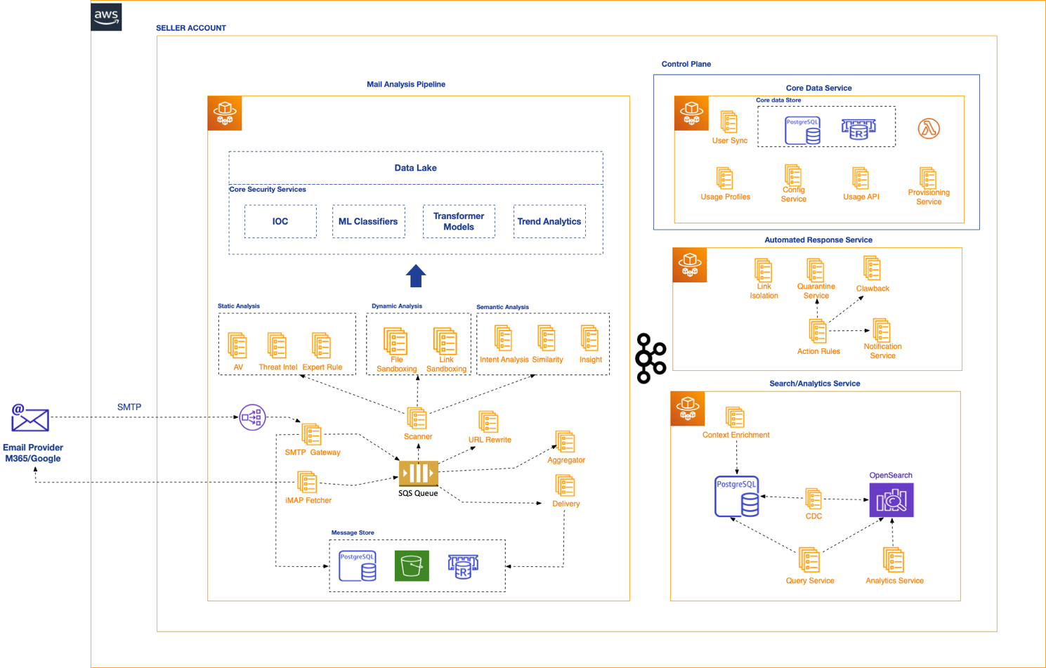
VIPRE IES architecture on AWS spanning data ingestion, AI and ML detection, response management, and search and analytics layers

Figure 1: VIPRE IES architecture on AWS

VIPRE IES uses a distributed, event-driven architecture specifically designed to identify and stop business email compromise and AI-generated phishing attempts. The system combines AI and ML technologies in a cost-effective manner to analyze and neutralize email-based risks. The architecture consists of four key layers:

Data ingestion

Processing millions of email messages reliably presents significant challenges, especially with unpredictable traffic spikes. VIPRE’s ingest mechanism uses AWS services to tackle this with a highly resilient system that maintains performance and availability regardless of volume.

  • Every incoming email stream is treated as a discrete job. The raw payload is immediately committed to Amazon S3 as an object. Amazon S3 delivers 99.999999999 percent (11 9s) durability, providing a reliable foundation for email payload storage.
  • The actual processing job (a lightweight reference pointing to the Amazon S3 object) is then queued in Amazon SQS, a fully managed message queuing service. This decoupling supports reliable message handling, buffers traffic spikes, and decouples ingestion from downstream processing.
  • Stateless microservices orchestrated by Amazon ECS with AWS Fargate for serverless container management, pull Amazon SQS jobs, fetch the Amazon S3 payload, and initiate the detection pipeline.

AI and ML detection with layered intelligence

After ingesting email data, the solution performs analysis using a multi-stage workflow where multiple engines are executed in parallel and phases are coordinated using fan-in and fan-out patterns. Based on how engines operate there are roughly four kinds of analysis done:

  1. Static analysis:
    • Engines in this category look at the email as passive data.
    • Definitions, rules, signatures, heuristics and classifiers are updated using hot reload.
  2. Behavioral analysis:
    • Various artifacts extracted from the email body (links, attachments) are opened in a controlled environment (also known as a sandbox) where the execution is monitored and passed through ML classifiers and other engines to identify unexpected behavior.
    • ML classifiers are versioned and shipped along with sandbox Docker images.
    • Heuristics and rule updates are done using Amazon S3 and Amazon S3 events.
  3. Semantic analysis:
    • Email text is passed through a pipeline for text understanding which uses multiple bi-directional transformer models to perform natural language processing (NLP) tasks such as named entity recognition and coreference, intent summarization, zero-shot classification, and semantic similarity matching.
    • The models used are strongly versioned, deployed in Docker images stored in Amazon Elastic Container Registry (Amazon ECR), using PyTorch and scheduled to execute on NVIDIA GPUs.
    • Heuristics and classified embedding datasets can be updated separately through packages stored in Apache Parquet format in Amazon S3, with Amazon Managed Workflows for Apache Airflow (Amazon MWAA) orchestrating data pipeline workflows.
  4. Apply contextual intelligence:
    • Global (customer independent) and local (customer dependent) data feeds are correlated and injected during analysis for context enrichment and detection.
      • Global: artifacts extracted from the email are checked against the latest emergent risks and IoCs, and verified against reputation and classification feeds.
      • Local: sender reputation, trust lists, roles, and similar signals are injected into the analysis context.
    • Intelligence collected by the system (discovered risks, regardless of the source) is fed back into the security data lake from where it’s available for rapid identification of emerging risks. Amazon CloudWatch provides centralized monitoring and governance across the entire detection pipeline.

Response management and remediation

This layer serves as the platform’s control plane, translating detection verdicts into automated actions based on customizable VIPRE IES Action Rule Definitions. Administrators can define specific match expressions against the aggregated threat model to trigger precise remediation workflows.

In inline mode, the service acts as a final gateway so that high-severity risks, such as confirmed malware or severe BEC, are quarantined and prevented from landing in the end-user’s mailbox. This immediate intervention keeps a risk’s dwell time minimal, neutralizing the concern instantly.

The service provides granular workflows for managing quarantined messages. These include:

  • Administrator release: Admins maintain full visibility, with the ability to review audit logs, engine scores, and raw payloads to safely release false positives.
  • End-user self-release: For lower-risk categories (for example, bulk mail), users receive a secure metadata digest so they can self-release items directly from a portal. This reduces administrative overhead while ensuring all user actions remain fully audited for review.

Post-delivery remediation (clawback)

Beyond inline blocking, the system uses native API integrations with mail providers to execute programmatic clawbacks. This allows the service to instantly retract malicious messages from user inboxes post-delivery, neutralizing “time-bomb” threats and preventing lateral movement.

By balancing immediate inline enforcement with flexible release workflows, the response and remediation service maximizes protection without disrupting legitimate business communication.

Search and analytics

This layer closes the loop, transforming the continuous stream of security telemetry into actionable, real-time intelligence for security operators.

  • Every state change and verdict across the entire system is published as an event to the Amazon MSK cluster. Amazon MSK provides the highly durable, ordered, and scalable event stream necessary to handle massive data velocity.
  • Events are consumed, contextually enriched with metadata (for example, user, group profile), and committed to Amazon Relational Database Service (Amazon RDS), which provides automated backups and high availability, to serve as the long-term, auditable system of record.
  • The system delivers instant search results by using change data capture (CDC) to stream updates from Amazon RDS in real time. This low-latency pipeline populates Amazon OpenSearch Service for sub-second analytical queries across security telemetry.
  • The search and analytics service exposes a powerful API that powers VIPRE’s dashboards and interactive reports. These perform sub-second, complex analytical queries that give security teams real-time visibility into their security posture and risk. Queries and results are strictly scoped by the client’s tenant ID, enforcing multi-tenant isolation and providing data separation assurance while supporting rapid incident response.

Real-world protection: how VIPRE IES stops advanced BEC incidents

VIPRE IES’s AI-powered detection successfully identifies and blocks sophisticated BEC and other evasive incidents that traditional email security would miss. Here’s how it works in real-world scenarios:

  • The “urgent wire transfer” incident: An employee in the accounting or finance department receives an email seemingly from their CEO or CFO. The email has a sense of urgency, stating a critical business deal requires an immediate wire transfer to a new vendor. VIPRE IES’s intent-aware AI classifies the email as a financial request, detects urgency triggers in language patterns, and identifies user impersonation along with other risk indicators to automatically quarantine the message.
  • The “confidential or legal matter” incident: An employee receives an email from what appears to be a senior leader or the legal department, with a subject line such as “Confidential Legal Matter – Attorney-Client Privilege.” The email asks the employee to provide sensitive information. VIPRE IES’s semantic analysis engine flags the use of emotionally charged, high-pressure language to create a false sense of urgency and secrecy.
  • The “thread hijacking” incident: When supply chain partners’ email accounts are compromised and actors insert fraudulent payment instructions into legitimate email threads, VIPRE’s conversation thread scoring and domain analysis immediately identify these sophisticated incidents, protecting against scenarios using fake message threads.
  • The “QR code (quishing)” scenario: A QR code incident (quishing) involves an actor embedding an image of a QR code into an email, often with a sense of urgency such as a “security update” or “password expiration,” to trick the recipient into scanning the code with their mobile device, which then directs them to a phishing site. VIPRE IES addresses this evasion by using multiple layers of advanced analysis including using image analysis to decode the URL and then perform real-time behavioral analysis of the URL in an isolated cloud sandbox.

These use cases demonstrate how VIPRE IES provides protection against the full spectrum of modern BEC incidents by applying multiple AI and ML detection layers to analyze message context, sender behavior, and communication patterns.

Results and impact

When you implement VIPRE IES, the combination of its advanced detection capabilities and its native AWS architecture provides a force-multiplier effect across three critical areas:

1. Neutralizing sophisticated BEC email

By using the elasticity of AWS compute to run deep AI and ML semantic analysis at scale, VIPRE IES successfully blocks sophisticated BEC incidents that bypass traditional security tools. This significantly reduces an organization’s exposure to financial fraud and wire transfer scams by identifying malicious intent in real time.

These capabilities are proven in production. In a sample 24-hour period across VIPRE’s Europe (EU) and North America (NA) production environments, VIPRE IES scanned 517,726 messages (376,847 in EU and 140,879 in NA) and detected 5,508 BEC attempts (3,853 in EU and 1,655 in NA). BEC attempts accounted for approximately 1 percent of all scanned messages. Each of those detections represents a potential fraud attempt identified by the system. This depth of analysis also operates at speed. P95 message-processing latency (hourly average) ranges from 1.4 to 15 seconds with dynamic sandboxing disabled, and from 39 to 78 seconds with full sandbox analysis enabled. This maintains real-time protection without disrupting legitimate mail flow.

2. Operational efficiency and reduced alert fatigue

The precision of the IES detection model, supported by the high-throughput processing of Amazon SQS, Amazon MSK, and Amazon ECS, means that security teams can focus on investigating genuine risks rather than managing false positives. This minimizes alert fatigue and supports a more proactive defense posture.

3. Accelerated time-to-protection

Because the platform is built on a cloud-native, API-driven framework, deployment is remarkably fast. Without the need for MX record changes, the solution can be deployed in minutes rather than days, accelerating protection while maintaining existing email infrastructure. This agility also provides immediate visibility into internal risks that traditional gateways often miss.

Beyond the immediate technical mitigation of BEC and zero-day threats, the platform’s native integration supports stringent enterprise compliance through robust encryption, granular role-based access control (RBAC), and comprehensive audit logging. These security improvements help rebuild trust in email communications across all levels of your organization, from end users to executive leadership.

Conclusion

Modern email threats outpace conventional security tools, creating dangerous blind spots in your defenses. Built on AWS services and using advanced AI and ML capabilities, VIPRE IES provides a cloud-native solution that protects against sophisticated BEC incidents. By offloading the “heavy lifting” of infrastructure to the global reach and elasticity of the AWS Cloud, VIPRE IES delivers a security fabric that is as resilient as it is precise.

VIPRE Security and AWS worked together to create a targeted solution that addresses specific email security challenges with precision and scalability. By removing the need for MX record changes and integrating directly with Microsoft 365, VIPRE IES offers a deployment path that accelerates time-to-value.

To get started with improving your email security:

  1. Review your current email security posture to identify gaps in BEC protection.
  2. Explore VIPRE IES in the AWS Marketplace to understand deployment options.
  3. Connect with AWS and VIPRE teams to discuss your specific security requirements.

Learn more about AWS security best practices and cloud-native email protection:

Learn more

VIPRE Security Group

VIPRE Security Group is a leading provider of internet security solutions that protect businesses and home users from cyber risks. For more than 25 years, VIPRE has provided one of the world’s largest intelligence clouds, delivering exceptional protection against today’s most aggressive online risks. The award-winning portfolio includes next-generation antivirus endpoint cloud and EDR solutions, MDR, pen-testing, advanced email security products, data loss awareness, intelligence for real-time malware analysis, and security awareness and compliance training.


About the authors

Bulk Executor for Amazon DynamoDB, Part 2: Lessons we learned the hard way

Post Syndicated from Jason Hunter original https://aws.amazon.com/blogs/architecture/bulk-executor-for-amazon-dynamodb-part-2-lessons-we-learned-the-hard-way/

In the Introducing open source Bulk Executor for Amazon DynamoDB blog post, you learned about the purpose and usage of the Bulk Executor tool. In this Part 2 post, we share the story of how we built it: the design tradeoffs, surprises, gotchas, and eventual workarounds. Think of it as your travel guide for working with Amazon DynamoDB and AWS Glue.

Design requirements

Bulk Executor is a project designed to run actions in bulk against many or all items in a table. For example you can mass delete old items or compare two tables for equality.

Three core requirements shaped most of the decisions that follow: running a bulk command should feel like a local script (real-time output, interruptible with ^C), it should scale to hundreds of parallel workers without the user managing infrastructure, and it should be straightforward to add new commands without tight coupling to the framework.

Selecting AWS Glue

We selected AWS Glue to drive the parallel execution. It’s a serverless service where you submit jobs that get distributed across workers (compute instances), each running tasks in parallel. For more information, see Key topics in Apache Spark. Our command-line client starts a job and AWS Glue handles distributing the work across potentially hundreds of workers.

We also considered Amazon Simple Queue Service (Amazon SQS) with AWS Lambda, AWS Fargate, Amazon EMR, and Ray. We decided to use AWS Glue because it gave us both serverless parallelism and a built-in DynamoDB connector, so we got much of the hard stuff at no cost. The following short code sample shows how to read or write items:

# Read from DynamoDB into a Spark DataFrame
dataframe = (
    spark.read
    .format("dynamodb")
    .option("dynamodb.input.tableName", "source")
    .option("dynamodb.throughput.read", "40000")
    .option("dynamodb.consistentRead", "false")
    .load()
)

# Write to DynamoDB from a Spark DataFrame
(
    dataframe.write
    .format("dynamodb")
    .option("dynamodb.output.tableName", "sink")
    .option("dynamodb.throughput.write", "40000")
    .option("dynamodb.item.size.check.enabled", "true")
    .save()
)

The Spark DataFrame gave us the built-in capabilities that we needed. Specifically:

  • A where/filter that accepts a Spark SQL condition to filter the data.
  • An orderBy that sorts the data.
  • A limit that controls the number of items.

On the back of these capabilities, we built the find command as our first command with its --where, --orderby, and --limit parameters requiring almost no coding on our part. If you want to print the 100 most recent undelivered orders, you can issue a bulk command like this:

./bulk find --table orders --where "status = 'undelivered'" --orderby timestamp desc --limit 100

The count command uses the same code but counts the items instead of printing them. The delete command does the same, but after finding the items runs parallel batch delete calls to remove them.

One downside of the Spark connector is that it doesn’t fully represent the source table data types. It simplifies the data and, for example, makes no distinction between a string set and a list of strings.

Estimating costs

When working against large tables, we wanted to give a cost estimate before starting the work. Predicting the future is always hard. Here’s how we did it.

For reads, we look at the table’s metadata (updated approximately every 6 hours, so beware a table that you recently loaded can read as smaller than it really is) to learn its recent size and calculate the read request units necessary for a full scan. For on-demand tables the math is straightforward: call the Pricing API to get the cost per million read request units for the region, multiply, done.

For provisioned mode, cost depends on the provisioned level, auto scaling headroom, and job duration, making estimation harder. Our heuristic is to take two-thirds of the on-demand price (divide by 1.5). The reasoning: a table provisioned at 100 percent utilization costs about 30 percent of the equivalent on-demand throughput. However, 100 percent is rarely achievable in practice. At 50 percent utilization, the cost is about 60 percent. We use 67 percent because it’s better to quote a little high.

For the delete command, write costs depend on how many items match, which we don’t know until after scanning. So delete calculates pricing in two phases: first the read cost estimate up front, then after finding the matches, the write cost based on the size of the deletion set.

For the fill command, which mass loads synthetic data according to a custom generator, we first generate some sample items to know the approximate size of the items, then price accordingly.

We don’t estimate AWS Glue Data Processing Unit (DPU) costs for two reasons. First, knowing how much compute will be required can’t be done simply. Second, we observed that for large jobs, DPU costs tend to be a small fraction of the DynamoDB costs. This makes sense, because an AWS Glue worker running at a small hourly cost can drive a huge amount of database activity. For small jobs, DPU is a larger fraction because of the overhead of getting things started, but the absolute dollars are low. You can specify --XWaitForDPU to see actual DPU costs reported after execution.

Every --X parameter is a parameter to the Bulk Executor itself, as opposed to the command being run. We modeled this after the Java Virtual Machine convention.

Job termination (^C)

We needed a way for the caller to terminate processing, for example if the pricing estimate comes back higher than expected. Pressing ^C stops the client Python script immediately but leaves the AWS Glue job running until its timeout.

We solved this by having the Python code catch the interrupt signal programmatically. An interrupt handler sees the ^C and sets an interrupted flag. This flag gets noticed by a watcher loop that’s always running. Usually it’s watching for things like AWS Glue state changes. But when it sees the interrupt, it actively directs the AWS Glue job to stop before proceeding with a clean exit of the client-side program. Now one ^C cleanly stops both sides.

Mandating point-in-time recovery (PITR)

A command like delete has the potential to delete more than anticipated. We made the design choice to require point-in-time recovery (PITR) to be enabled on any table receiving a mutating command. That way if your --where clause doesn’t do exactly what you wanted, you have a way to roll back.

This is one reason we built out the revert-export command to undo writes in place based on a PITR-driven incremental export. See our previous blog post “Recover from accidental DynamoDB changes using Bulk Executor”.

Watching execution (CloudWatch Live Tail)

In our first version, the client polled Amazon CloudWatch Logs for AWS Glue worker output. This was inefficient and meant output appeared delayed and in chunks. Switching to Amazon CloudWatch Live Tail let job output stream to the client in near real-time.

This introduced a problem: when find returned only a small number of matches things worked fine, but with large result sets we got incomplete output. The root cause: Live Tail displays at most 500 events per second. Beyond that, it streams only a sample of matching events.

Our solution was to write large output (from find or diff) to an Amazon Simple Storage Service (Amazon S3) bucket and only stream the first 10 results to the terminal, plus a link to the full data set.

Live Tail had two more surprises. Events can arrive out of order, so we built a reordering layer. Also, AWS Glue jobs can complete before their final log events appear in CloudWatch (there are a few seconds of propagation delay), so we couldn’t stop listening the moment the job stopped. We implemented a “microwave popcorn monitor”: stop listening only after a few seconds of silence.

Fast and useful error handling

When an AWS Glue task hits an error, it logs an exception and by default the stack trace goes into the logs for the client to see. If the error is in only one task, that’s manageable, if a bit verbose. But if it’s something that hits every task (like a bad --where clause), you get hundreds of identical stack traces flooding the terminal. We addressed this with four patterns.

On the client side, each command validates parameters before starting the AWS Glue job. A typo gets caught locally without AWS Glue ever spinning up.

Inside AWS Glue, we create an error_accumulator that’s a Spark accumulator. Instead of letting exceptions propagate up from tasks en masse, each task adds its exception to the accumulator. The Spark driver then extracts the first error and prints only that: one clean message instead of hundreds of duplicates, followed by a graceful job shutdown.

Continuously, on the client side, the Live Tail stream of events goes through a pattern matcher looking for error patterns that will never self-resolve (like AccessDeniedException, ModuleNotFoundError, OutOfMemoryError) and can trigger an immediate job stop rather than letting every task fail with the same error.

Also, to prevent “scary” stack traces for something as simple as a typo in a --where clause, we use a special app-specific exception type that a command can choose to throw when wanting to give an error and not a stack trace. Only developer-type errors should generate stack traces.

It took a while but we developed an approach to error handling that we liked: catch errors as quickly as possible, simplify them down to show the user only what’s necessary, and have the final line of each execution indicate if the job succeeded or failed (and why). We also added color coding (red for errors, yellow for warnings) to make issues easier to spot.

DynamoDB connector compared to direct access

The AWS Glue connector reads and writes DataFrames, but it has no way to delete items. For the delete command we had no choice but to make direct DynamoDB API calls. The command logic uses the connector to first find the matching items (giving a DataFrame), then iterates over the items to perform deletes using batch writes. Here’s a simplified version:

def delete_partition(partition, table_name, keys):
    table = dynamodb_resource.Table(table_name)
    with table.batch_writer() as batch:
        for record in partition:
            item = json.loads(record)
            key = {k: item[k] for k in keys}
            batch.delete_item(Key=key)

# Distribute deletes across workers
records.toJSON().foreachPartition(
    lambda partition: delete_partition(partition, table_name, keys)
)

Each Spark partition gets a slice of the matching items, and foreachPartition() runs the delete function in parallel across workers. The batch_writer() handles batching the individual deletes into efficient batch_write_item calls under the hood.

We built fill and load-export to write items directly by using batch_writer also, instead of constructing a DataFrame.

This pattern of going direct worked so well that it inspired us to rethink how we approached the first commands we wrote. We built a scancount command to explore whether counting could be faster without the connector.

The answer: consistently faster, because of less overhead. The connector-based count has to load every item into the AWS Glue context to then filter them and count what survived the filter. With scancount, we use DynamoDB segmented scan with push-down predicates and Select: COUNT so nothing comes out of the database except the count itself with the filter already having been applied. Each worker scans its own segment of the table in parallel:

def _count(table_name, index_name, filter_expression,
             segment, total_segments, total_matched_accumulator, error_accumulator):
    table = dynamodb_resource.Table(table_name)

    scan_kwargs = {
        "Select": "COUNT",
        "Segment": segment,
        "TotalSegments": total_segments
    }
    if index_name:
        scan_kwargs["IndexName"] = index_name
    if filter_expression:
        scan_kwargs["FilterExpression"] = filter_expression

    # Error handling code removed
    local_count = 0
    while True:
        response = table.scan(**scan_kwargs)
        local_count += response.get("Count", 0)
        if "LastEvaluatedKey" not in response:
            break
        scan_kwargs["ExclusiveStartKey"] = response["LastEvaluatedKey"]

    total_matched_accumulator.add(local_count)
    return local_count

parallelize_count = 100
rdd = spark_context.parallelize(range(parallelize_count), parallelize_count)
rdd.foreach(lambda worker_id: _count(table_name, index_name,
    filter_expression, worker_id, parallelize_count,
    total_matched_accumulator, error_accumulator))

The tradeoff: scancount accepts a raw --filter-expression instead of the higher-level --where Spark SQL syntax, since there’s no DataFrame involved.

The code for diff and copy also does direct reads instead of using the connector. With these commands, it wasn’t for speed but to make sure they keep perfect data type fidelity.

A side note on diff: it was important for each task to write its subset of output directly to its own Amazon S3 object, without ever centralizing the output back to the driver, which would not scale.

Rate limiting

The connector provides built-in rate limiting. However, for our commands making direct API calls (such as delete, fill, copy, and scancount), there’s no rate limiting. With enough AWS Glue workers running loops unconstrained, it usually generates unwanted throttles.

We built a distributed rate limiter that coordinates across all workers. The approach is described in detail in Rate-limiting calls to Amazon DynamoDB using Python Boto3, Part 1 and Part 2: Distributed Coordination.

Users control this with --XMaxReadRate and --XMaxWriteRate parameters. If unspecified, we investigate the environment to infer the appropriate rates based on account and table settings and quotas.

Recently, we added a feature to issue a (yellow) warning if the max read or write rate won’t allow the work to complete within the --XTimeout (which defaults to one hour). Better to warn the user early: if even the maximum rate can’t finish within the timeout, the user can restart with a higher rate or a longer timeout.

Building a library of commands

We started with the idea that commands should be straightforward to drop in, like new Unix commands. The loose coupling has paid off in contributions from outside the original core team. So far we’ve seen:

  • The diff command contributed by Chris Gillespie.
  • The sql command contributed by John Terhune.
  • The load command contributed by Arjan Schaaf.
  • The load-export and revert-export commands contributed by Ruskin Dantra.

Each command is its own Python module loaded by name. The contract is lightweight: export a run(job, spark_context, glue_context, parsed_args) function and use the shared conventions (the error_accumulator for exceptions, the distributed rate limiter for DynamoDB calls, and a shared library to help with cost estimates).

Upgrading to new AWS Glue versions, with the help of AI

A few months ago, we migrated from AWS Glue 4 to AWS Glue 5. The benefits: faster job startup and a new DynamoDB connector that loads directly into a DataFrame (the old connector required a DynamicFrame intermediate step, adding overhead and complexity).

The migration also gave us a chance to measure the new connector against the old one. We used AI tooling to generate a suite of stress tests comparing both connectors under AWS Glue 5, varying table sizes and read/write patterns. The AI ran these tests for hours, collected the results, and produced a comparison report that gave us the confidence the upgrade was worthwhile.

This migration had been on our backlog for a while and we kept postponing it. With AI handling the test generation and execution, we finished it in one interactive working session.

Since then we’ve upgraded to AWS Glue 6, this time to capture the 30 percent lower costs for DPU-hours.

Implementing an AI linter

We noticed some things are hard to test using either unit tests or end-to-end tests. For example, we have some data that exists in three places in three different formats, and we want to make sure those three definitions do not drift apart.

First, we have a README that explains some aspects of security. You can either let us generate a new AWS Glue job role for you, or you can pass in your own custom role by name. It explains, in English prose, the minimum AWS Identity and Access Management (IAM) permissions required by the AWS Glue job role if you create your own. That’s one definition.

The second definition is that when we create the role, we attach the right set of permissions on the role. The third definition is that when you provide the role we check the role’s effective permissions (partly through the IAM policy simulator and partly by reading its attached policies) to confirm that you’ve given the role the proper minimum. This follows the principle that we should error out early here if not, instead of on first execution.

It would be a bad and subtle bug if, as the permissions requirements change, any of the three differently-formatted statements of the same core facts diverge. It’s not easy to compare English prose with role-creating logic with IAM-checking logic.

Our solution was to create an AI linter. It’s a folder in the project with a README that defines the linter behavior and a subfolder with a set of rules each held as a markdown file. When desired, we can ask AI to run the linting. No coding required.

Other rules we have say that every command (including commands in the future) should impose rate limiting, whether through the connector or Python library. That’s not easy to test, but easy for AI to reason about. Another rule is every command with large output must write the output to Amazon S3 (following a particular location selection convention) and output to the terminal a bounded preview with a link.

Any false alarms are only informative to us as a development team, and we can refine the rules to remove them. Of course, AI authored the markdown files themselves too.

Conclusion

None of the problems we solved were individually massive. They were all little things: Live Tail sampling events, ^C not reaching the remote job, error messages repeating hundreds of times, not knowing costs in advance, unbounded read and write rates. But each one made the tool frustrating to use until we fixed it. If you’re building your own tooling on AWS Glue, we hope these solutions save you some discovery time. We also hope our experience using AI for long-running or hard-to-run tests gives you some ideas.

The project is open source on GitHub and we welcome contributions. Now that you’ve seen the internals, you have everything you need to write your own commands. Write the run() function and rely on the harness for the rest. If you think it’s generally useful, send us a pull request!


About the authors

[$] Owning C types from Rust code

Post Syndicated from daroc original https://lwn.net/Articles/1099015/

Rust’s system of ownership and borrowed references is convenient when it can
correctly model a program’s needs. The

Rust for Linux project
has worked to
provide adapters between Rust’s semantics and the existing C code
in the kernel. At Kangrejos 2026, Andreas Hindborg spoke about a

patch
series
implementing the next such adaptor: an Ownable trait for
representing objects that are allocated in C code, but which Rust code is responsible
for cleaning up (if not necessarily deallocating) when it is done with them.
He hoped to finally reach a consensus on the patch series, after months of
discussion on the mailing list.

Eisentraut: The reverts will continue until morale improves

Post Syndicated from jzb original https://lwn.net/Articles/1100182/

PostgreSQL core
team member
Peter Eisentraut has written a blog
post
reflecting on the “unusually high number of features” that have
been taken out of the upcoming PostgreSQL 19 release since the beta period
began.

Some of the reverted features had significant architectural defects that
would have been hard to fix quickly and during beta. But there was also a long
tail of relatively harmless issues involving various edge cases. In past times,
many of these would not have surfaced until much later and we would have fixed
them bit by bit over the subsequent five years. But with LLM-assisted code
review, these kinds of things can get found much faster, and then you’re staring
at a list of like forty defect reports. And even if each of them requires only a
three-line fix on average, there is a fixed overhead to dealing with each of
these, and then you run out of time. Most if not all of the affected reverted
features were written a long time ago when LLM-assisted code review was not as
useful as it is now, meaning that the effective quality bar has been raised
after the time the feature was written and committed. Unless the capabilities of
LLM-assisted code review keep improving at the current rate, this situation
should sort itself out for future development cycles.

A corollary of that is that, at least for the most part, as far as I can
tell, this situation is not due to “vibe coding”. This code was written well
before that was a possibility.

LWN covered the unusually
large number of bug fixes required for PostgreSQL 19 features in
September.

Security updates for Tuesday

Post Syndicated from jzb original https://lwn.net/Articles/1100181/

Security updates have been issued by AlmaLinux (cjose, curl, emacs, environment-modules, flatpak, flatpak-builder, gd, glibc, kernel, libxml2, pcre2, and rsyslog), Debian (chromium, keystone, libgit2, librsvg, nagios4, and ntfs-3g), Fedora (baresip, bcm283x-firmware, curl, flare-im, GitPython, iperf3, kernel, libebml, libmatroska, libre, mkvtoolnix, python-mkdocs-rss-plugin, radicale, uboot-tools, and xiphos), Mageia (antlr4-project, cjose, cups, firefox, nss, golang, libextractor, nginx, ntfs-3g, openvpn, perl-DBI, perl-Imager, polkit, rsync, strongswan, thunderbird, tor, ugrep, vlc, and wireshark), Oracle (bind, bind9.16, cjose, compat-openssl10, compat-openssl11, curl, dovecot, emacs, flatpak, jackson-core, jackson-databind, jackson-jaxrs-providers, and jackson-modules-base, kernel, mod_auth_openidc, nodejs:22, tftp, and thunderbird), SUSE (bind, gcc13, gcc48, ghostscript, go1.26, go1.27, helm, libpng16, librsvg, libsoup, libX11, libXi, python, python-anyio, python-Django, python-PyJWT, python-tornado6, python-urllib3, python310, python313-bugzilla, python313-cmarkgfm, python313-colander, python313-configobj, python313-confluent-kafka, python313-django-registration, python313-ecdsa, python313-httptools, python313-imagecodecs, python313-impacket, terraform-provider-aws, terraform-provider-azurerm, terraform-provider-external, terraform-provider-google, terraform-provider-helm, terraform-provider-kubernetes, terraform-provid, thunderbird, unbound, virtiofsd, and xorg-x11-server), and Ubuntu (ffmpeg, google-guest-agent, google-osconfig-agent, and libx11).

Признаване на имунизации от чужбина и опитът за промени в една наредба

Post Syndicated from Боян Юруков original https://yurukov.net/blog/2026/vaksini-chujbina/

Днес ми попадна обществено обсъждане на предложение за промени в наредба, които засягат имунизациите на деца в чужбина. Тъй като съм се сблъсквал с този проблем се зачетох. Наистина има нормативен вакум в това отношение и с връщането на все повече семейства в страната темата става все по-належаща.

Моят опит беше, че се върнахме малко преди началото на първи клас. Дъщеря ми имаше всички ваксини според тогавашния календар в Германия и няколко препоръчителни. Това означаваше, че имаше ваксина срещу менингококи B и рота вирус, когато още не бяха широко разпространени в България, но нямаше срещу туберкулоза, тъй като не се прилага в Германия. Всичко беше въведено в международната имунизационна книжка, която е стандартна там, както и в повечето държави по света. Когато трябваше да вадим бележка за училище, дадохме тази книжка на личния лекар. БЦЖ ваксината беше поставена като дойде време да правим манту.

Процес за това обаче няма. Няма и общи препоръки какво да се прави когато дете е имунизирано по чужд календар, който се различава от българския. Например, в Германия слагат МПР ваксините на 11 и 15 месеца заедно с ваксината за варицела. В България се слагат на 13 месеца и 11 или 12 години. Дъщеря ми имаше две дози и се допитахме до РЗИ дали има нужда да слагаме дозата на 12 години. чудиха се и в крайна сметка препоръчаха да я сложим, тъй като не пречи. Аз аналогично се реимунизирах на 30 години след серия от локални епидемии от морбили в Германия, защото моят като деца са ми сложили само една доза.

Какво предлагат МЗ?

Промените са всъщност в наредба за прием в детски градини. Това е първият им порок. Не решава генерално казуса с ваксини поставени в чужбина или липсата им при пренасяне в България. Аналогични проблеми има при прием в ясла и училище, последното от които се сблъсках аз. Тоест потенциално трябва да правят подобни предложения в други наредбаи, които вероятно да имат различен процес.

Вторият проблем е, че вменяват задължение на РЗИ-тата да решават случай по случай дали да се признят ваксини поставени в чужбина. Това е отчасти иронично предвид намеренията на сегашния кабинет да закрива РЗИ. В същото време предвиждат, че личният лекар може да направи такова становище, но само ако е поставил/а някаква ваксина от българския календар. Това като условие е повече от странно предвид, че личният лекар отговаря по начало за здравето на детето и изготвя служебни бележки за състоянието му независимо дали е поставял ваксина или не. Отделно, за да се приеме дете в градина, то трябва да има личен лекар така или иначе, защото само такъв може да издава бележка. Проблем е, че не дават и срок, в който РЗИ следва да вземе решение поставяйки в риск кандидатстването за общински заведения. Отчитат в мотивите, че вероятно РЗИ-тата нямат капацитет, но никъде не правят анализ колко такива случая се очакава да има на година и за какво натоварване следва да се готвят.

Проблем е и втората точка, в която изискват заклет превод с нотариална заверка на подписа на преводача. Първо, налагало ми се е да превеждам медицински документи и за целта трябва специализирани преводачи, които са малко, концентрирани в големите градове и услугите им струват значително повече. Второ, нотариалната заверка на превода и самият превод са напълно излишни. Не знам за лекар, който да не знае латинските или английските имена на болестите, срещу които се имунизираме, но най-вече важното в случая са имената на препаратите. Това всъщност споменават и в проекта. Имената не се превеждат също катко и датите на поставянето им. Приета практика почти навсякъде е да се лепят отрязък от етикета с името и сериен номер за проследяване в имунизационните картони. По имената се разбира за какво е ваксината, още повече, че са регистрирани централно. Това е напълно достатъчно да се разбере кога какви ваксини за какво са сложени. Нищо в превода, заклетия преводач или нотариалната заверка не предпазва от грешки при разчитане на книжката или от документални измами. Ако книжката няма лепенки от ваксините, а са написани на ръка, може би има смисъл от превод и разчитане, но отново нотариалната заверка не помага за някаква сигурност. Имам и съмнение, че никой лекар няма да приеме написан на ръка картон по този начин съдейки от разговорите ми днес.

Липсата на срокове и уточнение кога се прилага това изискване са огромна пречка. В предложението пише, че се отнася до първи прием в градина. Не става ясно дали се отнася до конкретна или градина като цяло. Смяната на градини не е рядка в големите градове и по мои наблюдения познавайки доста семейства върнали се от чужбина е дори по-често сред тях особено в началото. Така разписана точката може да се разчете от директорите на градините, че при всяка смяна трябва да се мине през РЗИ за становище. Това добавя към и без това излишната административна тежест за родители и администрация.

Предложнията не определеят и какво следва да се случи при установяване на пропуск в имунизациите – било то заради отказ от ваксини, липса на достъп до адекватно здравеопазване или в по-честия случай разминаване в календарите. Не е определено дали РЗИ със становището си следва да направи препоръка как да навакса. Не е вмемено задължение за указания или стандарти за личните лекари, когато те изготвят такива становища.

Този и други пропуски в процеса излизат от целта на наредбата, защото проблемът далеч не е само с приема в детска градина. Това предложение е единствено и само бюрократична кръпка за конкретен казус.

Алтернативно предложение

Когато минавах сам през тази ситуация питах лекари, РЗИ, НЗОК и НЗИС как може да се въведат тези ваксини в електронния картон. По онова време имаше три различни системи, в които се въвеждаха ваксини – НЗОК, НЗИС и една пилотна на НЦЗПБ, но сега вече всичко е в НЗИС. Беше ми отговорено, че там може да се въвеждат само тези поставени лично от лекар. В това има логика, но следва същият начин на мислене наследен от НЗОК, които проследяваха какво е платено, а не здравето на хората.

В случая може да се разшири системата да се въвеждат ваксини на база чуждестранни документи като се отбележи, че ваксината е поставена от друг лекар по чужд календар и се прикачи снимка на въпросния документ за справка на други лекари. Ще е буквално две полета в базата в повече. Това въвеждане може да се прави от личния лекар или РЗИ и ще следва логиката на становището за признаване на имунизации от чужбина, която е разписана в предложението на МЗ.

Това ще реши веднъж за винаги проблема с липсващите ваксини. Ще може служебно да се проверява дали детето отговаря на всички изисквания за превантивна грижа не само за градината, но и за ясла и училище. Ще се прави веднъж, а не да се рискува при всяка смята да искат ново становище. Най-вече ще може да се проследи колко деца имат ваксини поставени по различен календар и при промяна на препоръките – например, че е добра идея да се сложи МПР на 12 години, а някое от РЗИ-тата е решило различно – може да се свържат с родителите.

Вероятно ще има критика, че това може да доведе до злоупотреби, в които лични лекари да въвеждат служебно ваксини уж, че са поставени в чужбина. В действителност, сегашното предложение на МЗ носи именно такъв риск, тъй като всеки лекар може да сложи – включително фиктивно – една ваксина и да отпише другите. Всичко това остава на хартия и се използва единствено за прием в градината. При моя вариант се въвежда някаква проследимост, в която се вижда точно кой ги е признал и на база какви документи. При концентрация на такива случаи с анализ на данните може да се открият системни нарушители.

Ролята на РЗИ в този процес следва да бъде както и сега на надзор и препоръки. Вместо да разглеждат всеки отделен случай, следва личните лекари да се допитват при особени такива. В общия случай обаче следва да се издадат препоръки към лекарите на база сравнение на календарите поне в рамките на ЕС. При въвеждане на данните в НЗИС проверката може да става служебно и автоматично на база тези правила и препоръки дори. Няма нужда родителите да ходят изрично и да чакат становище. По-добре би било самите лекари да отбелязват на база изготвените препорък и при нужда допитвания до РЗИ, че ваксините въведени по описания горе начин се приемат за еквивалентни на календара в България.

Какво следва?

Предложението е на етап обществено обсъждане до 11-ти ноември. Описах критиките си към него и препоръките си в коментар към това обсъждане. Ако сте съгласни и/или имате какво да добавите, добра идея е да напишете своя обратна връзка там, за да се обърне внимание. Похвално е, че най-накрая е намерен капацитет да се обърне внимание на този нормативен пропуск. Решението на МЗ създава повече трудности от проблема прибягвайки към чисто бюрократични способи и мислене.

Ако се приеме в този си вид, рискуваме една от първите срещи на връщащите се в България семейства да е с процедуален абсурд, излишни разходи и загуба на време за нещо тривиално. Споменават същото, впрочем, в доводите си и фактът, че го приемат за нормално или неизбежно отговаря на въпроса защо виждаме всички недъзи описани до тук.

Тук трябва да се спомене, че нито предложението на МЗ, нито това, което аз предлагам засягат системен проблем с липса на имунизации и проследяване на здравното състояние на деца, които често се местят през граница. Проблемът засяга основно семейства в риск включително мигранти. Не е уникален до България, а централен проблем в Европа поради практическата липса на обмен на информация не само между държавите, а често и в тях. Наредба за прием в градина няма да обхване тези деца, защото немалко от тях няма да тръгнат на градина. Здравната система в другите държави не ги обхваща, защото понякога не знае, че са там. В България също нямаме инфорамция, че са извън страната докато не стане време да тръгнат на училище и учители или социални работници започват да ги издирват. Този проблем съществува включително в рамките на страната ни с ширещата се сегрегация в училищата, проблемите с достъпа до здравеопазване и най-вече наличието на лични лекари, проблемите с гражданската регистрация и здравното образование. Един регистър или наредба няма да оправят това, но е проблем, за който трябва да признаем и да започнем да говорим.


Повече по темата с българите в чужбина, градините и имунизациите:

CVE-2026-97229: Critical Unauthenticated Remote Code Execution in GitLab

Post Syndicated from Rapid7 original https://www.rapid7.com/blog/post/etr-cve-2026-97229-critical-unauthenticated-remote-code-execution-in-gitlab

Overview

On October 12, 2026, GitLab published a critical patch release for CVE-2026-97229, an integer overflow or wraparound (CWE-190) in the CI/CD regular expression compiler affecting GitLab Community Edition (CE) and Enterprise Edition (EE). GitLab assigned the vulnerability a CVSSv3.1 score of 10.0. Under certain conditions, a remote attacker can execute arbitrary code on an affected GitLab server through a specially crafted regular expression stored in a malicious CI/CD configuration. While the vendor supplied CVSS score indicates that exploitation is fully unauthenticated, in reproducing the exploit it was noted that an attacker must have a mechanism to plant a malicious CI/CD configuration to a repository prior to triggering the vulnerability. On GitLab instances where new users can self register and create projects, this constraint is removed.

The vulnerability affects self-managed GitLab instances across all deployment types. GitLab.com is already running a patched version, and GitLab Dedicated customers do not need to take action.

As of this writing, there is no confirmed in-the-wild exploitation of CVE-2026-97229. However, Rapid7 Intelligence has independently reproduced arbitrary code execution on an unpatched, official GitLab CE image. Given the vulnerability’s maximum CVSS score, network-accessible trigger, and code execution in a GitLab application worker, Rapid7 recommends upgrading affected self-managed instances on an urgent basis, outside of normal patch cycles.

Technical overview

Rapid7’s testing found that an attacker must first be able to commit a malicious CI/CD configuration file .gitlab-ci.yml, and a repository path containing UTF-8 characters to a branch in a public project. For example, an ordinary account can satisfy this prerequisite by creating a public project on a self-managed GitLab instance where that functionality is permitted. 

The crafted regular expression initially compiles in a compact US-ASCII representation and passes GitLab’s regular expression validation. When it is evaluated against a specially formed, valid UTF-8 repository path, Ruby’s Onigmo regular expression engine recompiles it for the new encoding after those checks have completed. An integer overflow in the compiler’s program-size calculation then causes invalid regular expression instructions to be generated. The resulting loss of control-flow integrity can be used to execute attacker-controlled Onigmo VM operations in the Ruby process and run an operating system command as the GitLab git user.

Rapid7 validated the complete chain against the official GitLab 19.4.1 CE Linux amd64 image with address space layout randomization enabled. The same input did not execute against the official patched 19.4.2 CE image. Further root cause and exploit-chain details will be included in a separate Rapid7 technical analysis.

Mitigation guidance

A vendor-provided patch is available to remediate CVE-2026-97229. Organizations running affected self-managed GitLab CE or EE instances should immediately upgrade to a fixed version, without waiting for a regular patch cycle:

Affected GitLab CE/EE versions

Fixed version

All versions from 19.2 before 19.2.8

19.2.8

All versions from 19.3 before 19.3.5

19.3.5

All versions from 19.4 before 19.4.2

19.4.2

GitLab.com has already been updated, and GitLab Dedicated customers do not need to take action. Until affected self-managed instances can be upgraded, restricting anonymous access to public projects and preventing untrusted users from creating or writing to public projects can reduce exposure to the exploit path demonstrated by Rapid7. These controls address only the demonstrated delivery path and do not remediate the vulnerable regular expression compiler.

For the latest mitigation guidance, please refer to GitLab’s security advisory.

Rapid7 customers

Exposure Command, Vulnerability Management, and Nexpose

Exposure Command, Vulnerability Management, and Nexpose customers can assess exposure to CVE-2026-97229 with an authenticated vulnerability check expected to be available in today’s (October 13) content release.

Updates

  • October 13, 2026: Initial publication.

GrabMart data for faster disease outbreak detection

Post Syndicated from Grab Tech original https://engineering.grab.com/grabmart-data-for-faster-disease-outbreak-detection

Abstract

Retail purchases can supplement clinical surveillance because changes in demand for some over-the-counter (OTC) products may appear before confirmed case reports. This article describes an early-stage concept for analysing aggregated GrabMart transaction data to identify unusual changes in product demand. The concept is not a deployed system, and it would require validation by public health experts, privacy review, and regulatory approval before any implementation.

Introduction

Public health agencies use sources such as clinical case reports, laboratory results, and hospital records to monitor disease activity. Retail data may offer an additional signal when demand changes across groups of symptom-related products. It cannot establish a diagnosis or replace clinical evidence.

When using indirect signals, we should assess whether they remain relevant to the outcome we want to measure. This includes considering how changes in user behaviour could affect their interpretation. A retail-based signal can experience similar drift, selection bias, and false alarms. Any useful design must therefore combine statistical validation with careful privacy and governance controls.

Background

Syndromic surveillance tracks patterns that may indicate emerging illness before diagnoses are confirmed. Retail surveillance applies this idea to changes in demand for products associated with symptoms, such as fever remedies or cough medicines.

The proposed method groups eligible products into broad symptom classes and measures changes in aggregate demand over time. An anomaly score can indicate that observed demand differs from an expected seasonal pattern. The score is a statistical signal, not an estimate of how many people have a disease.

The design uses the following terms:


Proposed solution

The proposed pipeline would process only transactions that meet documented eligibility rules. It would map eligible SKUs to symptom classes, aggregate counts across approved time periods and geographic areas, and compare each series with an appropriate baseline. Public health experts would review the resulting Early Outbreak Detection Index alongside independent evidence.

The method deliberately excludes identity linkage and individual-level health inference. It also avoids using a single purchase to classify a customer, target an advertisement, adjust an insurance decision, or change access to a product.

Conceptual data flow

Eligible transactions
        |
        v
Reviewed SKU-to-symptom mapping
        |
        v
Aggregate by approved time period and geographic area
        |
        v
Compare with seasonal and historical baselines
        |
        v
Privacy and quality checks
        |
        v
Aggregate signal for authorised public health evaluation

Analysis and validation

Several statistical methods could model expected demand, including seasonal time-series models and spatial scan statistics. Model selection should follow retrospective evaluation against approved public health data. Evaluation should measure sensitivity, false-alert rate, calibration, geographic stability, and performance during seasonal changes.

The system would also need ongoing monitoring. Product catalogues change, purchasing behaviour shifts, promotions affect demand, and access to GrabMart varies across populations and locations. These factors can produce anomalies unrelated to disease activity.

Privacy and governance

Privacy protection starts with data minimisation. The analysis should use only eligible product categories, coarse geographic areas, and aggregate time windows approved for the stated public health purpose. It should not expose raw transactions or personally identifiable information (PII).

The release process could apply minimum-count thresholds and differential privacy (DP), subject to a documented privacy analysis. Privacy specialists would need to set and review any privacy budget. Access controls, retention limits, audit logs, and contractual restrictions would govern any approved data exchange.

An independent review should cover privacy law, health-related inference, fairness, scientific validity, and the risk of harm from false alerts. An authorised public health body, rather than an automated model, should decide whether and how to communicate a possible outbreak.

Potential applications

If research validates the signal and the required approvals are in place, aggregate trends could support:

  • public health research alongside established surveillance sources;
  • operational planning for broad categories of health supplies; and
  • evaluation of whether retail demand contributes useful evidence during an emerging event.

These applications should use aggregate trends only. The signal should not drive personalised medical advice, individual targeting, insurance decisions, or automatic changes to medicine search rankings.

Limitations

Retail demand is an indirect and incomplete measure of illness. Purchases may reflect promotions, weather, media coverage, household stocking, or changes in product availability. GrabMart customers are not representative of the full population, and the available product mix differs by market.

Mapping a product to a symptom class is also uncertain because many products have several uses. Aggregation and privacy controls reduce disclosure risk but can weaken statistical utility. These limitations require local validation and documented thresholds before anyone interprets the index.

Conclusion

Aggregated retail transactions may add a timely signal to public health research, but they cannot replace clinical surveillance. A responsible design must minimise data, prohibit individual health inference, test the model against independent evidence, and place public health experts in control of interpretation and communication.

This concept remains in the early planning phase. No production deployment, measured performance result, or public health integration is claimed.

Join us

Grab is a leading superapp in Southeast Asia, operating across the deliveries, mobility, and digital financial services sectors. Serving over 900 cities in eight Southeast Asian countries: Cambodia, Indonesia, Malaysia, Myanmar, the Philippines, Singapore, Thailand, and Vietnam. Grab enables millions of people every day to order food or groceries, send packages, hail a ride or taxi, pay for online purchases or access services such as lending and insurance, all through a single app. We operate supermarkets in Malaysia under Jaya Grocer and Everrise, which enables us to bring the convenience of on-demand grocery delivery to more consumers in the country. As part of our financial services offerings, we also provide digital banking services through GXS Bank in Singapore and GXBank in Malaysia. Grab was founded in 2012 with the mission to drive Southeast Asia forward by creating economic empowerment for everyone. Grab strives to serve a triple bottom line. We aim to simultaneously deliver financial performance for our shareholders and have a positive social impact, which includes economic empowerment for millions of people in the region, while mitigating our environmental footprint.

Powered by technology and driven by heart, our mission is to drive Southeast Asia forward by creating economic empowerment for everyone. If this mission speaks to you, join our team today!

The collective thoughts of the interwebz