Use Amazon Redshift Spectrum with row-level and cell-level security policies defined in AWS Lake Formation

Post Syndicated from Anusha Challa original https://aws.amazon.com/blogs/big-data/use-amazon-redshift-spectrum-with-row-level-and-cell-level-security-policies-defined-in-aws-lake-formation/

Data warehouses and data lakes are key to an enterprise data management strategy. A data lake is a centralized repository that consolidates your data in any format at any scale and makes it available for different kinds of analytics. A data warehouse, on the other hand, has cleansed, enriched, and transformed data that is optimized for faster queries. Amazon Redshift is a cloud-based data warehouse that powers a lake house architecture, which enables you to query the data in a data warehouse and an Amazon Simple Storage Service (Amazon S3) data lake using familiar SQL statements and gain deeper insights.

Data lakes often contain data for multiple business units, users, locations, vendors, and tenants. Enterprises want to share their data while balancing compliance and security needs. To satisfy compliance requirements and to achieve data isolation, enterprises often need to control access at the row level and cell level. For example:

  • If you have a multi-tenant data lake, you may want each tenant to be able to view only those rows that are associated to their tenant ID
  • You may have data for multiple portfolios in the data lake and you need to control access for various portfolio managers
  • You may have sensitive information or personally identifiable information (PII) that can be viewed by users with elevated privileges only

AWS Lake Formation makes it easy to set up a secure data lake and access controls for these kinds of use cases. You can use Lake Formation to centrally define security, governance, and auditing policies, thereby achieving unified governance for your data lake. Lake Formation supports row-level security and cell-level security:

  • Row-level security allows you to specify filter expressions that limit access to specific rows of a table to a user
  • Cell-level security builds on row-level security by allowing you to apply filter expressions on each row to hide or show specific columns

Amazon Redshift is the fastest and most widely used cloud data warehouse. Amazon Redshift Spectrum is a feature of Amazon Redshift that enables you to query data from and write data back to Amazon S3 in open formats. You can query open file formats such as Parquet, ORC, JSON, Avro, CSV, and more directly in Amazon S3 using familiar ANSI SQL. This gives you the flexibility to store highly structured, frequently accessed data in an Amazon Redshift data warehouse, while also keeping up to exabytes of structured, semi-structured, and unstructured data in Amazon S3. Redshift Spectrum integrates with Lake Formation natively. This integration enables you to define data filters in Lake Formation that specify row-level and cell-level access control for users on your data and then query it using Redshift Spectrum.

In this post, we present a sample multi-tenant scenario and describe how to define row-level and cell-level security policies in Lake Formation. We also show how these policies are applied when querying the data using Redshift Spectrum.

Solution overview

In our use case, Example Corp has built an enterprise data lake on Amazon S3. They store data for multiple tenants in the data lake and query it using Redshift Spectrum. Example Corp maintains separate AWS Identity and Access Management (IAM) roles for each of their tenants and wants to control access to the multi-tenant dataset based on their IAM role.

Example Corp needs to ensure that the tenants can view only those rows that are associated to them. For example, Tenant1 should see only those rows where tenantid = 'Tenant1' and Tenant2 should see only those rows where tenantid = 'Tenant2'. Also, tenants can only view sensitive columns such as phone, email, and date of birth associated to specific countries.

The following is a screenshot of the multi-tenant dataset we use to demonstrate our solution. It has data for two tenants: Tenant1 and Tenant2. tenantid is the column that distinguishes data associated to each tenant.

To solve this use case, we implement row-level and cell-level security in Lake Formation by defining data filters. When Example Corp’s tenants query the data using Redshift Spectrum, the service checks filters defined in Lake Formation and returns only the data that the tenant has access to.

Lake Formation metadata tables contain information about data in the data lake, including schema information, partition information, and data location. You can use them to access underlying data in the data lake and manage that data with Lake Formation permissions. You can apply row-level and cell-level security to Lake Formation tables. In this post, we provide a walkthrough using a standard Lake Formation table.

The following diagram illustrates our solution architecture.

The solution workflow consists of the following steps:

  1. Create IAM roles for the tenants.
  2. Register an Amazon S3 location in Lake Formation.
  3. Create a database and use AWS Glue crawlers to create a table in Lake Formation.
  4. Create data filters in Lake Formation.
  5. Grant access to the IAM roles in Lake Formation.
  6. Attach the IAM roles to the Amazon Redshift cluster.
  7. Create an external schema in Amazon Redshift.
  8. Create Amazon Redshift users for each tenant and grant access to the external schema.
  9. Users Tenant1 and Tenant2 assume their respective IAM roles and query data using the SQL query editor or any SQL client to their external schemas inside Amazon Redshift.

Prerequisites

This walkthrough assumes that you have the following prerequisites:

Create IAM roles for the tenants

Create IAM roles Tenant1ReadRole and Tenant2ReadRole for users with elevated privileges for the two tenants, with Amazon Redshift as the trusted entity, and attach the following policy to both roles:

{
	"Version": "2012-10-17",
	"Statement": [{
		"Effect": "Allow",
		"Action": [
			"lakeformation:GetDataAccess",
			"glue:GetTable",
			"glue:GetTables",
			"glue:SearchTables",
			"glue:GetDatabase",
			"glue:GetDatabases",
			"glue:GetPartition",
			"glue:GetPartitions"
		],
		"Resource": "*"
	}]
}

Register an Amazon S3 location in Lake Formation

We use the sample multi-tenant dataset SpectrumRowLevelFiltering.csv. Complete the following steps to register the location of this dataset in Lake Formation:

  1. Download the dataset and upload it to the Amazon S3 path s3://<your_bucket>/order_details/SpectrumRowLevelFiltering.csv.
  2. On the Lake Formation console, choose Data lake locations in the navigation pane.
  3. Choose Register location.
  4. For Amazon S3 path, enter the S3 path of your dataset.
  5. For IAM role, choose either the AWSServiceRoleForLakeFormationDataAccess service-linked role (the default) or the Lake Formation administrator role mentioned in the prerequisites.
  6. Choose Register location.

Create a database and a table in Lake Formation

To create your database and table, complete the following steps:

  1. Sign in to the AWS Management Console as the data lake administrator.
  2. On the Lake Formation console, choose Databases in the navigation pane.
  3. Choose Create database.
  4. For Name, enter rs_spectrum_rls_blog.
  5. If Use only IAM access control for new tables in this database is selected, uncheck it.
  6. Choose Create database.Next, you create a new data lake table.
  7. On the AWS Glue console, choose Crawlers in navigation pane.
  8. Choose Add crawler.
  9. For Crawler name, enter order_details.
  10. For Specify crawler source type, keep the default selections.
  11. For Add data store, choose Include path, and choose the S3 path to the dataset (s3://<your_bucket>/order_details/).
  12. For Choose IAM Role, choose Create an IAM role, with the suffix rs_spectrum_rls_blog.
  13. For Frequency, choose Run on demand.
  14. For Database, choose database you just created (rs_spectrum_rls_blog).
  15. Choose Finish to create the crawler.
  16. Grant CREATE TABLE permissions and DESCRIBE/ALTER/DELETE database permissions to the IAM role you created in Step 12.
  17. To run the crawler, in the navigation pane, choose Crawlers.
  18. Select the crawler order_details and choose Run crawler.When the crawler is complete, you can find the table order_details created under the database rs_spectrum_rls_blog in the AWS Glue Data Catalog.
  19. On the AWS Glue console, in the navigation pane, choose Databases.
  20. Select the database rs_spectrum_rls_blog and choose View tables.
  21. Choose the table order_details.

The following screenshot is the schema of the order_details table.

Create data filters in Lake Formation

To implement row-level and cell-level security, first you create data filters. Then you choose that data filter while granting SELECT permission on the tables. For this use case, you create two data filters: one for Tenant1 and one for Tenant2.

  1. On the Lake Formation console, choose Data catalog in the navigation pane, then choose Data filters.
  2. Choose Create new filter.
    Let’s create the first data filter filter-tenant1-order-details restricting the rows Tenant1 is able to see in table order_details.
  3. For Data filter name, enter filter-tenant1-order-details.
  4. For Target database, choose rs_spectrum_rls_blog.
  5. For Target table, choose order_details.
  6. For Column-level access, select Include columns and then choose the following columns: c_emailaddress, c_phone, c_dob, c_firstname, c_address, c_country, c_lastname, and tenanted.
  7. For Row filter expression, enter tenantid = 'Tenant1' and c_country in  (‘USA’,‘Spain’).
  8. Choose Create filter.
  9. Repeat these steps to create another data filter filter-tenant2-order-details, with row filter expression tenantid = 'Tenant2' and c_country in (‘USA’,‘Canada’).

Grant access to IAM roles in Lake Formation

After you create the data filters, you need to attach them to the table to grant access to a principal. First let’s grant access to order_details to the IAM role Tenant1ReadRole using the data filter we created for Tenant1.

  1. On the Lake Formation console, in the navigation pane, under Permissions, choose Data Permissions.
  2. Choose Grant.
  3. In the Principals section, select IAM users and roles.
  4. For IAM users and roles, choose the role Tenant1ReadRole.
  5. In the LF-Tags or catalog resources section, choose Named data catalog resources.
  6. For Databases, choose rs_spectrum_rls_blog.
  7. For Tables, choose order_details.
  8. For Data filters, choose filter-tenant1-order-details.
  9. For Data filter permissions, choose Select.
  10. Choose Grant.
  11. Repeat these steps with the IAM role Tenant2ReadRole and data filter filter-tenant2-order-details.

Attach the IAM roles to the Amazon Redshift cluster

To attach your roles to the cluster, complete the following steps:

  1. On the Amazon Redshift console, in the navigation menu, choose CLUSTERS, then select the name of the cluster that you want to update.
  2. On the Actions menu, choose Manage IAM roles.The IAM roles page appears.
  3. Either choose Enter ARN and enter an ARN of the Tenant1ReadRole IAM role, or choose the Tenant1ReadRole IAM role from the list.
  4. Choose Add IAM role.
  5. Choose Done to associate the IAM role with the cluster.The cluster is modified to complete the change.
  6. Repeat these steps to add the Tenant2ReadRole IAM role to the Amazon Redshift cluster.

Amazon Redshift allows up to 50 IAM roles to attach to the cluster to access other AWS services.

Create an external schema in Amazon Redshift

Create an external schema on the Amazon Redshift cluster, one for each IAM role, using the following code:

CREATE EXTERNAL SCHEMA IF NOT EXISTS spectrum_tenant1
FROM DATA CATALOG DATABASE 'rs_spectrum_rls_blog'
IAM_ROLE '<<Tenant1ReadRole ARN>>'
REGION 'us-east-1';

CREATE EXTERNAL SCHEMA IF NOT EXISTS  spectrum_tenant2
FROM DATA CATALOG DATABASE  'rs_spectrum_rls_blog'
IAM_ROLE '<<Tenant2ReadRole ARN>>'
REGION 'us-east-1';

Create Amazon Redshift users for each tenant and grant access to the external schema

Complete the following steps:

  1. Create Amazon Redshift users to restrict access to the external schemas (connect to the cluster with a user that has permission to create users or superusers) using the following code:
    CREATE USER tenant1_user WITH PASSWORD '<password>';
    CREATE USER tenant2_user WITH PASSWORD '<password>';

  2. Let’s create the read-only role (tenant1_ro) to provide read-only access to the spectrum_tenant1 schema:
    create role tenant1_ro;

  3. Grant usage on spectrum_tenant1 schema to the read-only tenant1_ro role:
    grant usage on schema spectrum_tenant1 to role tenant1_ro;

  4. Now assign the user to the read-only tenant1_ro role:
    grant role tenant1_ro to tenant1_user;

  5. Repeat the same steps to grant permission to the user tenant2_user:
    create role tenant2_ro;
    grant usage on schema spectrum_tenant2 to role tenant2_ro;
    grant role tenant2_ro to tenant2_user;

Tenant1 and Tenant2 users run queries using the SQL editor or a SQL client

To test the permission levels for different users, connect to the database using the query editor with that user.

In the Query Editor in the Amazon Redshift console, connect to the cluster with tenant1_user and run the following query:

-- Query table 'order_details' in schema spectrum_tenant1 with role Tenant1ReadRole

SELECT * FROM spectrum_tenant1.order_details;

In the following screenshot, tenant1_user is only able to see records where the tenantid value is Tenant1 and only the customer PII fields specific to the US and Spain.

To validate the Lake Formation data filters, the following screenshot shows that Tenant1 can’t see any records for Tenant2.

Reconnect to the cluster using tenant2_user and run the following query:

-- Query table 'order_details' in schema spectrum_tenant2 with role Tenant2ReadRole

SELECT * FROM spectrum_tenant2.order_details;

In the following screenshot, tenant2_user is only able to see records where the tenantid value is Tenant2 and only the customer PII fields specific to the US and Canada.

To validate the Lake Formation data filters, the following screenshot shows that Tenant2 can’t see any records for Tenant1.

Conclusion

In this post, you learned how to implement row-level and cell-level security on an Amazon S3-based data lake using data filters and access control features in Lake Formation. You also learned how to use Redshift Spectrum to access the data from Amazon S3 while adhering to the row-level and cell-level security policies defined in Lake Formation.

You can further enhance your understanding of Lake Formation row-level and cell-level security by referring to Effective data lakes using AWS Lake Formation, Part 4: Implementing cell-level and row-level security.

To learn more about Redshift Spectrum, refer Amazon Redshift Spectrum Extends Data Warehousing Out to Exabytes—No Loading Required.

For more information about configuring row-level access control natively in Amazon Redshift, refer to Achieve fine-grained data security with row-level access control in Amazon Redshift.


About the authors

Anusha Challa is a Senior Analytics Specialist Solutions Architect at AWS. Her expertise is in building large-scale data warehouses, both on premises and in the cloud. She provides architectural guidance to our customers on end-to-end data warehousing implementations and migrations.

Ranjan Burman is an Analytics Specialist Solutions Architect at AWS.

[$] What’s in a (type) name?

Post Syndicated from original https://lwn.net/Articles/906496/

The kernel’s manual
pages
are in a bit of an interesting position. They
are managed as a separate project, distinct from the kernel’s
documentation, and have the task of documenting both the kernel’s
system-call interface and the wrappers for that interface provided by the C
library. Sometimes the two objectives come into conflict, as can be seen
in a discussion that has been playing out over the course of the last year
on whether to use C standard type names to describe kernel-defined
structures.

Montenegro Is the Victim of a Cyberattack

Post Syndicated from Bruce Schneier original https://www.schneier.com/blog/archives/2022/09/montenegro-is-the-victim-of-a-cyberattack.html

Details are few, but Montenegro has suffered a cyberattack:

A combination of ransomware and distributed denial-of-service attacks, the onslaught disrupted government services and prompted the country’s electrical utility to switch to manual control.

[…]

But the attack against Montenegro’s infrastructure seemed more sustained and extensive, with targets including water supply systems, transportation services and online government services, among many others.

Government officials in the country of just over 600,000 people said certain government services remained temporarily disabled for security reasons and that the data of citizens and businesses were not endangered.

The Director of the Directorate for Information Security, Dusan Polovic, said 150 computers were infected with malware at a dozen state institutions and that the data of the Ministry of Public Administration was not permanently damaged. Polovic said some retail tax collection was affected.

Russia is being blamed, but I haven’t seen any evidence other than “they’re the obvious perpetrator.”

EDITED TO ADD (9/12): The Montenegro government is hedging on that Russia attribution. It seems to be a regular criminal ransomware attack. The Cuba Ransomware gang has Russian members, but that’s not the same thing as the government.

Architecting for Extortion: Acting on the IST’s Blueprint for Ransomware Defense

Post Syndicated from Erick Galinkin original https://blog.rapid7.com/2022/09/02/architecting-for-extortion-acting-on-the-ists-blueprint-for-ransomware-defense/

Architecting for Extortion: Acting on the IST’s Blueprint for Ransomware Defense

Last month, the Institute for Security and Technology’s (IST) Ransomware Task Force (RTF) launched the Blueprint for Ransomware Defense, a mitigation, response, and recovery plan for small- and medium-sized enterprises. This action plan is a cross-industry document that targets business leaders and protectors to ensure that even resource-strapped organizations can defend against the continued threat of extortion attacks, including ransomware.

Crucially, the RTF understands that most teams are strapped for resources, including time. So while it can be incredibly insightful — and great fun — to sketch out taxonomies of ransomware actors and their TTPs, or do graph analysis on communications networks for cybercrime groups, the blueprint considers what they call “essential cyber hygiene,” the foundational capabilities needed to successfully combat ransomware and other extortion threats.

A note on terminology

The term “ransomware” refers to a type of malware that encrypts files and demands payment for the key necessary to decrypt the files. A trend pioneered by the Maze ransomware group in 2020, double extortion, adds a second layer to this by also exfiltrating files and threatening to leak them if the ransom is not paid. We’ve also begun to see a broader trend of hack-and-leak extortion operations typified by the now-defunct LAPSU$ group, where rather than performing double extortion, the attacker simply skips the ransomware step of the operation.

While the Ransomware Task Force — as its name suggests — has prioritized ransomware, and the blueprint is called the Blueprint for Ransomware Defense, the overwhelming majority of the safeguards are useful against a variety of attacks. Thus, when we say “ransomware,” we specifically mean “an attack in which your files are encrypted and a ransom is demanded” and “extortion” for the broader class of operations.

How to use the blueprint

The blueprint outlines 40 safeguards: 14 foundational and 26 actionable. The foundational safeguards are the well-trod security advice that protectors are familiar with: Have an asset inventory, have a vulnerability management process, establish a security awareness program, etc.

Readers who wish to review these safeguards should consult the RTF blueprint directly and particularly consider printing out Appendix A, which nicely lists the category and type of each safeguard while also mapping it to the National Institute of Standards and Technology (NIST) cybersecurity framework function and the Center for Internet Security (CIS) safeguard number. There is also a helpful tools and resources spreadsheet linked in the PDF.

Safeguards to start implementing today

All of the safeguards chosen by the RTF are designed to be easy to implement and offer good “bang for your buck.” The controls that RTF has identified as important have also been identified by CIS as crucial for stopping ransomware attacks. However, some items, such as having a detailed asset inventory, are easier said than done. Of these, a handful are uniquely impactful or easy to implement, so they offer a good starting point.

1. Require MFA for externally exposed applications, remote network access, and administrative access

OK, technically this recommendation is three safeguards, but since they’re related, we’re lumping them into one. Lumping these together does not mean that implementation is a one-stop shop. Indeed, each one of these will require its own configuration to get working. However, as our incident response analysts and pentesters can both attest, the number one headache for attackers is multi-factor authentication (MFA).

MFA may not be a panacea, but it can serve as a roadblock for initial access or lateral movement, and it can provide an early warning that someone is in your environment who does not belong. If your organization is not pushing MFA everywhere, they should be, as most enterprise applications today support it natively or via single sign-on. A variety of free and paid authenticators exist and can be implemented in a straightforward manner.

2. Restrict administrator privileges to dedicated administrator accounts

Separation of duties is a longstanding core tenet of information security, but between remote work, the increased speed of communications and development, and the general expectation that things Get Done Right Now, we have systematically over-privileged user accounts. Even if global administrators remain rare, users are often local administrators on their machines, permitting the installation of unauthorized software that can be used by attackers and access brokers to establish persistence. This persistence can be leveraged into higher-level access through the use of tools like Mimikatz or techniques like Kerberoasting, and that higher-level access exposes the enterprise to significant risk.

By restricting administrator privileges to dedicated accounts, we develop some very clear indicators that something is wrong – no administrator account should ever be logged in multiple places at the same time, and there are some functions that simply should never be performed from a dedicated administrator account. This may add some friction to your IT management, but it’s good friction.

3. Use DNS filtering services

Unlike the two previous suggestions, this is something that not only could you start implementing today – you could probably finish implementing it today. Domain Name System (DNS) filtering services replace the default DNS configuration in your environment. Free options like Quad9 and OpenDNS offer security-friendly domain name lookups, which can defeat phishing attempts, malvertising, and malware command and control beaconing.

CIS also offers malicious domain blocking and reporting to members of some organizations. In general, this is a simple configuration update that can be pushed to all computers and will instantly improve your security posture.

Safeguards for tomorrow

While the three action items for today will offer the greatest return on investment for your time, all of the safeguards in the guide are important. Many are well-understood but can take time to implement. For some controls that aren’t “table stakes” in the way that deploying anti-malware software, establishing a security awareness program, and collecting audit logs are, we offer a bit of advice.

1. Manage default accounts on enterprise assets and software

As Rapid7’s own Curt Barnard demonstrated with Defaultinator this year at Black Hat, applications and hardware are still rife with default credentials that never get changed. Defaultinator is one tool that can help evaluate devices that may have default credentials in use. Finding these default accounts can be challenging, but once you have a good asset inventory, managing these default accounts is important to keeping attackers out and your data in.

2. Use unique passwords

Continuing with the notion of credentials, using unique passwords is incredibly important. Password reuse is a common way for attackers to move from a single, potentially unrelated account to your crown jewels. Today, there are myriad password management tools that will even generate unique passwords for users and many of them offer enterprise subscriptions. Of these, nearly all allow for the secure sharing of passwords – if for some reason that is necessary. (Hint: It’s almost never actually necessary, but merely a bad habit.) Easily guessable (or easily shareable) passwords often fall victim to brute-force or password-spraying attacks, and with an enterprise password management tool, no user should need to use passwords that aren’t both strong and unique.

3. Establish and maintain a data management process

While we all know the power, benefit, and value of backups – especially when it comes to ransomware – data management is a bit more nuanced. We know that attackers in double extortion or leak-and-extort operations choose the files they steal and leak carefully to put maximum pressure on victims. Thus, the data management process is of increased importance for this category of attack. Categorizing and classifying your data will help inform the particular restrictions that need to be put around that data. Since attackers are targeting and leaking different sorts of data across industries, it’s imperative to know what data is most important to you and most likely to be targeted by attackers, and to have a plan to protect it.

While extortion attacks are on the rise and ransomware remains an expensive threat to organizations, action plans like the RTF’s Blueprint for Ransomware Defense serve as great tools to help decision makers, technical leaders, and other protectors mitigate extortion attacks. The safeguards in the report and the details in this blog post can help prioritize and contextualize what needs to be done. After all, we’re all targets, but we don’t all have to be victims.

Additional reading:

NEVER MISS A BLOG

Get the latest stories, expertise, and news about security today.

Git’s database internals V: scalability

Post Syndicated from Derrick Stolee original https://github.blog/2022-09-02-gits-database-internals-v-scalability/

This week, we are exploring Git’s internals with the following concept in mind:

Git is the distributed database at the core of your engineering system.

When the database at the core of an application approaches scale limits of a single database node, a common strategy is to shard the database. By splitting the database into multiple components, we can scale beyond the limits of a single node.

For Git, large repositories can have a similar feeling. While there exist some extremely large monorepos operating with success, they require careful attention and advanced features. For some, that effort is better spent sharding the repository. Just like sharding an application database, there are many ways to split a Git repository, with various trade-offs.

When sharding an application database, there are a number of factors to consider.

Some application databases include automatic horizontal sharding based on a shard key, which is usually a string literal that can be sorted lexicographically so related values appear in the same shard due to a common prefix in the shard key. There is no immediate way to shard Git’s object store in this way. The object IDs are hashes of the object contents and have essentially random prefixes.

Instead, we think of sharding strategies that split the repository by other structures, including logical components, paths in the worktree, and time periods in the commit history.

Component sharding: multi-repo

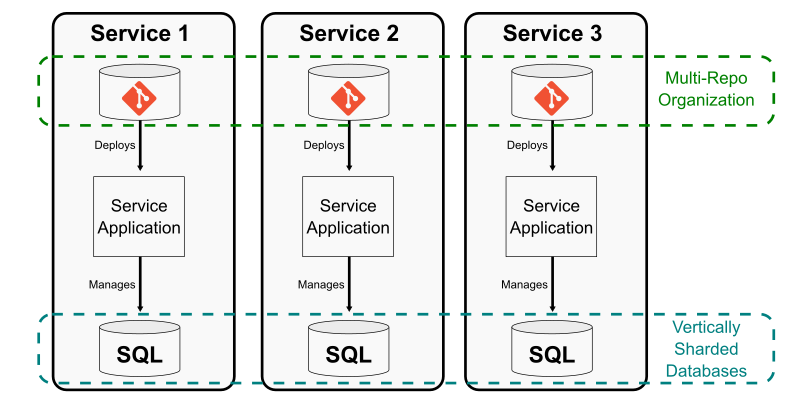
One way to shard an application database is to split out entire tables that can be operated independently and managed by independent services. The Git equivalent is to split a repository in to multiple smaller repositories with no concrete links between them. This creates a multi-repo sharding strategy.

The common approach to this strategy is to extract functionality out of a monolith into a microservice, but that microservice exists in its own Git repository that is not linked at all to the monolith’s repository. This effort might remove code from the monolith across multiple path prefixes due to the monolith’s architecture.

Multi-repo sharding strategy that extracts functionality out of a monolith into a microservice that exists in its own Git repository.

Using this strategy works best if each microservice is paired with a team that manages that repository, including full responsibility for developing, testing, deploying, and monitoring that service. This is very similar to the application database sharding strategy, where there is typically one application component connected to that database shard. There is no need for other components to be aware of that database since it is hidden by the component interface.

Multi-repo environments work best when there is a similar “human abstraction” where the team is autonomous as long as their service satisfies certain contracts that other teams depend on.

The tricky part of the multi-repo setup is that it requires human overhead to track where these component repositories live and how they link together. The only way to link the connections of the larger service ecosystem is through documentation and siloed experiential knowledge. System-wide efforts, such as security audits, become difficult to track to completion.

Another main downside to the multi-repo organization is that shared dependencies become difficult to manage. Common dependencies must be imported using package managers instead of using source control updates. This can make it difficult to track the consumers of those dependencies, leading to a lack of test coverage when updating those core components.

The next sharding strategy solves some of these multi-repo issues by collecting all of the smaller repositories into one larger super-repository.

Horizontal sharding: submodules

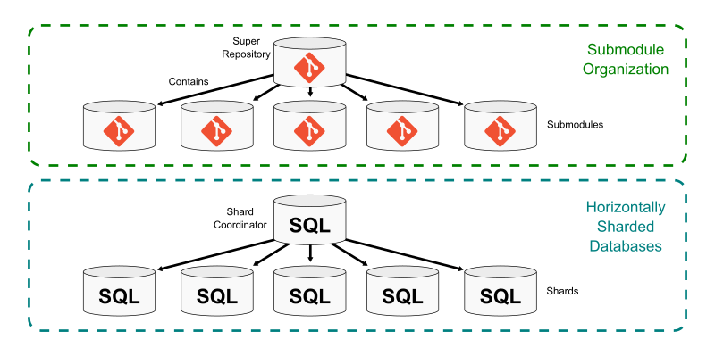
Git submodules allow a repository to include a link to another repository within its worktree. The super repository contains one or more submodules at specific paths in the worktree. The information for each submodule is stored in the .gitmodules file, but the tree entry for that submodule’s path points to a commit in the submodule repository.

Submodules create a way to stitch several smaller repositories into a single larger repository. Each has its own distinct commit history, ref store, and object store. Each has its own set of remotes to synchronize. When cloning the super repository, Git does not recursively clone the submodule by default, allowing the user to opt-in to the submodules they want to have locally.

One main benefit of using a super repository is that it becomes the central hub for finding any of the smaller repositories that form a multi-repo setup. This is similar to a horizontally sharded application database that uses a shard coordinator database to actively balance the shards and run queries on the correct shard.

Diagram showing how a Git super repository can become the central hub for finding any of the smaller repositories that form a multi-repo setup.

Further, certain global properties can be guaranteed via continuous integration builds such as cross-submodule source dependencies. In this setup, the super project creates requirements that it cannot advance a submodule unless all builds and tests in the super project pass. This creates some safety that a core component does not break any consumer in the super project.

This global structure has a cost. The submodule repositories become less independent. Since they have their own Git hosting location, users can update them by pushing changes. This can even be done with local builds that make sure that component is self-consistent. However, any update to the submodule repository is incomplete until the super project updates its path pointer to that commit. At the same time, should the submodule repository move forward before that change has been validated within the super repository?

This contention between the independence of the submodule repository and the inter-dependence of submodules in the super repository is a major hurdle. It is up to the architects of this arrangement to create policies and procedures to ensure that all of the components interact well with the entire system.

One common issue developers have in a submodule environment is when there is a source dependency across multiple submodules. If a breaking change is introduced in one submodule repository, the consumer repositories need to be updated to take advantage of those changes. However, this means that all of the submodules need to coordinate when they are updated into the super repository.

There are a lot of tools out there in the wild to help manage submodules, all built on top of the git submodule command. One famous example is Google’s repo tool that coordinates changes across multiple submodules.

If you are interested in submodules and super repository workflows, then you would likely benefit from coming to Git Merge 2022 (or, watching the videos afterward), especially Emily Shaffer’s talk, “An Improved Workflow for Submodules.”

Using a single worktree: Monorepos

The previous two examples focused on reducing the size of Git repositories by breaking them up based on the worktree. By having fewer files in each repository, fewer developers are interacting with each and the repositories grow more slowly. Each approach had its benefits and trade-offs, and one big issue with each was build-time source dependencies between components.

Another common way to avoid source dependencies across multiple repositories is to only have one repository: a monorepo. Here, I’m defining a monorepo as a repository containing all source code required to build and ship a large system. This does not mean that every single file written by an employee of the company must be tracked in “the monorepo.” Instead, monorepos are defined by their strategy for how they choose to include components in the same repository:

If it ships together, it merges together.

One pattern that is increasing in popularity is the service-oriented architecture (SOA) monorepo. In this environment, all of the code for the application is contained in the same repository, but each component deploys as an independent service. In this pattern, each component can be tested against the current version of all of the other services before it is deployed.

The monorepo pattern solves many of the coordination issues discussed in the previous sharding strategies. The biggest downside is that the repository itself grows very quickly. As discussed in the previous parts of this series, Git has many advanced features that improve performance even for large repositories. Monorepos more frequently need to enable those advanced Git features, even for client repositories.

One of the main costs of a monorepo is actually the build system. If every change to the monorepo requires passing builds across the entire system, then the build system needs to take advantage of incremental builds so updates to a single component do not require building the entire monorepo. Most groups using large monorepos have a team dedicated to the developer experience, including improving the build system. Frequently, these build improvements can also lead to being able to use advanced Git features such as sparse-checkout and partial clone, which can greatly reduce the amount of data necessary for client repositories to interact with the monorepo.

Even with a carefully designed architecture and the best Git features available, monorepos can still grow incredibly fast. It may be valuable to take a monorepo and find creative ways to split it and reset the size to something smaller.

Time-based sharding

One solution to a fast-growing monorepo is to consider it as if it was a time-series database: the changes over time are important, so what if it shards based on time instead of based on the worktree?

When performing a time-based shard, first determine a point in time where the existing monorepo can be paused and all movement on the trunk branch can be blocked. Pausing work on a monorepo is very unusual, so should be done with extreme care and preparation.

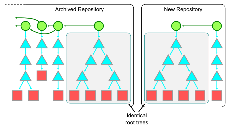
After pausing the changes to the monorepo’s trunk, create a new repository with the same root tree as the current trunk of the old monorepo, but with a brand new root commit. Be sure to reference the old monorepo and its tip commit somewhere in the message of that new root commit. This commit can be pushed to a new repository.

Diagram representing the time-based sharding strategy.

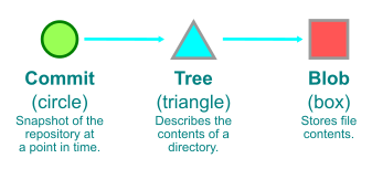
For a quick refresher on how we represent Git objects, see the key below.

Key to how Git objects are represented. A green circle represents a commit; a blue triangle represents a tree; and a red box represents a blob.

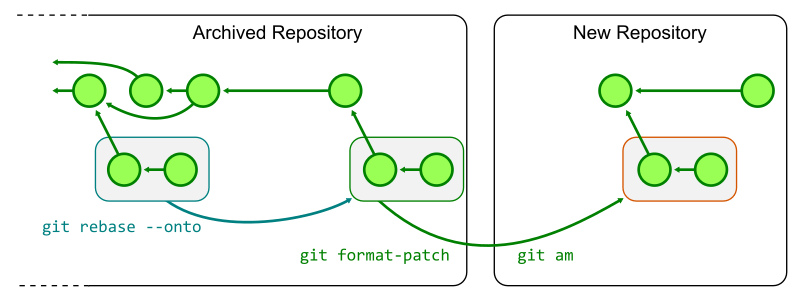
Any ongoing work in the old monorepo must be replayed on top of the new repository. One way to do this is to rebase each topic branch onto the final commit of the trunk branch, then generate patches with git format-patch and then apply those patches in the new repository with git am.

Diagram representing how ongoing work in the old monorepo is replayed on top of the new repository using rebasing and patches.

After the new monorepo shard is created, the old monorepo can be archived as a read-only repository as all new work continues in the new monorepo. There are likely many updates required to ensure that everyone knows the new monorepo location as well as repository secrets to update. If your repository uses infrastructure as code patterns, then almost all of the information for building, testing, and deploying the monorepo will automatically be ready in the new monorepo.

Even with all of these precautions, performing a time-based shard like this is disruptive and requires a timeframe where no new work is merging into the trunk. If you are considering doing this in your engineering system, then I highly recommend doing a few test runs to make sure you minimize the time between locking the old shard and deploying out of the new shard.

The biggest benefit of this approach is that it can be done at any time regardless of the shape of your worktree. The other sharding methods require some amount of architecture changes in order to split into multiple repos or submodules. This approach cuts out the potentially large commit history and all of the old versions of files without changing the repository structure at the tip.

A time-based shard might be particularly beneficial if your commit history includes some anti-patterns for Git repositories, such as large binary files. If you have done the hard work to clean up the worktree at the tip of your repository, you may still want to clear those old files. This sharding approach is similar to rewriting history, except that the new monorepo can have an even smaller size.

However, that commit history from the old monorepo is still important! We just discussed commit history and file history queries in this blog series. It is extremely important to be able to find the reasons why the code is in its current form. In the new monorepo shard, it will look like the entire codebase was created in a single commit!

To satisfy these history queries, Git can combine the two histories in a way that allows a seamless history query, though at some performance cost. The good news is that these history queries across the shard boundary may be common at first, but become less common as time goes on.

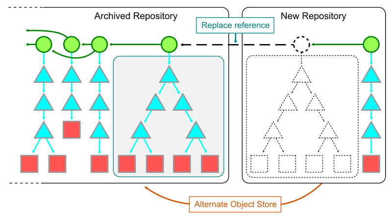
The first step to combining the two shards together is to have a local clone of each. In the new shard, add the object store of the old repository as a Git alternate. Add the full path to the .git/objects directory of the old repository into the .git/objects/info/alternates file in the new repository. While this file exists, it allows Git processes in the new repository to see the objects in the old one.

The second step is to use git replace to create a reference that tells Git to swap the contents of the new root commit with the tip of the old repository. Since those commits share the same root tree, the only change will be the message and commit parents at that point. This allows walking “through” the link into the previous commit history.

Strategy for combining two shards together by having a local clone of each.

It is important to note that operating with replace objects enabled comes at some performance cost. In addition to having the large commit history that existed before the split, some features like the commit-graph file discussed in part II are not compatible with replace objects. For this reason, operating in this combined mode should only be done when it is critical to do history queries across the shard boundary.

One way to guarantee that the combined history is quickly available, but does not affect normal Git operations is to “hide” the replace references using the GIT_REPLACE_REF_BASE environment variable. This writes the replace reference in a non-standard location, so the replacement is only effective when that environment variable is set to your custom value.

Using replace references to view a combined form of the history can also help transition ongoing work from the old repository to the new one. While in the combined mode, users can use git rebase to move their topics from the old history to the new history. They no longer need to use the git format-patch and git am transformation.

Here is a concrete example for how I created a time-based shard of the Git repository starting at the v2.37.0 tag:

$ git init
$ echo /home/stolee/_git/git/src/.git/objects >.git/objects/info/alternates

$ git commit-tree -m "new root commit" \
                  -m "Sharded from e4a4b31577c7419497ac30cebe30d755b97752c5" \
                  -m "Signed-off-by: Derrick Stolee <[email protected]>" \
                  a4a2aa60ab45e767b52a26fc80a0a576aef2a010
b49d35c8288501462ca1a008b3bb2efb9b4c4a9d

$ GIT_REPLACE_REF_BASE=refs/shard git replace \
                  b49d35c8288501462ca1a008b3bb2efb9b4c4a9d \
                  e4a4b31577c7419497ac30cebe30d755b97752c5

$ git log --oneline
b49d35c828 (HEAD -> master) new root commit

$ GIT_REPLACE_REF_BASE=refs/shard git log --oneline -n 5
b49d35c828 (HEAD -> master, replaced) Git 2.37
49c837424a Merge branch 'jc/revert-show-parent-info'
5dba4d6540 Merge tag 'l10n-2.37.0-rnd1' of https://github.com/git-l10n/git-po
fc0f8bcd64 revert: config documentation fixes
71e3a31e40 l10n: sv.po: Update Swedish translation (5367t0f0u)

You can follow the instructions in the sharded repository to experience cloning the two repositories and using the combined history as needed.

Time-based shards can be successful in reducing several dimensions of scale that cause friction in a large monorepo. However, the hurdle of transitioning work to a new repository location may be too disruptive for your group. There is one final sharding strategy I’ll discuss today, and it keeps the logistical structure of the monorepo in a single location while still improving how client repositories interact with the remote repository.

Data offloading

When a database grows, it may be beneficial to recognize that some data elements are infrequently accessed and to move that data to less expensive, but also lower performance storage mechanisms. It is possible to do this with Git repositories as well!

It is possible to think about partial clone as a way to offload data to secondary storage. A blobless clone (created by git clone --filter=blob:none) downloads the full commit history and all reachable trees from the origin server, but only downloads blob contents when necessary. In this way, the initial clone can be much faster and the amount of local storage greatly reduced. This comes at a cost that when Git needs a blob to satisfy a git checkout or git blame query, Git needs to communicate across the network to get that information. Frequently, that network hop requires going great distances across the internet and not just a local area network.

This idea of offloading data to secondary storage can work even better if there is a full clone of the remote repository available to add as an alternate. Perhaps the repository lives on a network fileshare that is accessible on the local network. Perhaps your IT department sets up new machines with a hard-disk drive containing a static copy of the repository from certain points in time. In either case, a blobless partial clone can add that static repository as an alternate, providing a faster lookup location for the blobs that do not exist in the local object store.

One major benefit of this kind of setup is that most custom query indexes, such as the commit-graph and changed-path Bloom filters, work automatically in this environment. This can be a great way to bootstrap local clones while minimizing the effect of missing blobs in a partial clone.

However, the current organization only helps at clone time. All fetches and future operations still grow the local repository size at the same rate, without ever reducing the size of the repository.

It is possible to take this idea of data offloading and use it to move data out of your local repository and into secondary storage, freeing up your expensive-but-fast storage for cheap-but-slower storage.

The key idea is again to use Git alternates, and create an alternate that points to some area of secondary storage. The second step is to discover objects in the repository history that are infrequently used, then copy them to that alternate and delete them from the local copy.

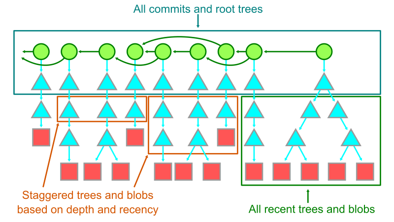
To decide what is an “infrequently used” object, we can use the commit history. The commits themselves are cheap and used for many commit history queries, so always keep those in the local storage. Similarly, keep each root tree. Also, objects reachable from recent root trees should be kept locally. (Feel free to be flexible to what you think “recent” means.)

After we know that we care about these objects, there are many ways we can decide what else should be kept. We could have a hard cutoff where we only keep root trees and no other objects older than that cutoff. We could also taper off the object list by first moving the blobs older than the cutoff, then slowly removing trees at certain depths, keeping fewer and fewer trees as the history gets older and older. There are a lot of possibilities to explore in this space.

Diagram representing secondary storage offloading based on recency.

I don’t know of any existing tool that does this kind of secondary storage offloading based on recency, but I think it could be really useful for some of these large monorepos. If this is something you think would work for your team, then try building it yourself tailored to your specific needs. Just promise that you’ll tell me if you do, because I want to see it!

Let’s keep the conversation going!

Thank you for reading this blog series! I had a lot of fun writing it and thinking about these advanced Git features and some potential extensions.

This may be the end of my prepared writing, but I will keep thinking of Git like a database for a very long time. If you have additional ideas to share, then please ping me on Twitter so we can keep the conversation going. I’ll also be speaking at Git Merge 2022 covering all five parts of this blog series, so I look forward to seeing you there!

A multi-dimensional approach helps you proactively prepare for failures, Part 3: Operations and process resiliency

Post Syndicated from Piyali Kamra original https://aws.amazon.com/blogs/architecture/a-multi-dimensional-approach-helps-you-proactively-prepare-for-failures-part-3-operations-and-process-resiliency/

In Part 1 and Part 2 of this series, we discussed how to build application layer and infrastructure layer resiliency.

In Part 3, we explore how to develop resilient applications, and the need to test and break our operational processes and run books. Processes are needed to capture baseline metrics and boundary conditions. Detecting deviations from accepted baselines requires logging, distributed tracing, monitoring, and alerting. Testing automation and rollback are part of continuous integration/continuous deployment (CI/CD) pipelines. Keeping track of network, application, and system health requires automation.

In order to meet recovery time and point objective (RTO and RPO, respectively) requirements of distributed applications, we need automation to implement failover operations across multiple layers. Let’s explore how a distributed system’s operational resiliency needs to be addressed before it goes into production, after it’s live in production, and when a failure happens.

Pattern 1: Standardize and automate AWS account setup

Create processes and automation for onboarding users and providing access to AWS accounts according to their role and business unit, as defined by the organization. Federated access to AWS accounts and organizations simplifies cost management, security implementation, and visibility. Having a strategy for a suitable AWS account structure can reduce the blast radius in case of a compromise.

  1. Have auditing mechanisms in place. AWS CloudTrail monitors compliance, improving security posture, and auditing all the activity records across AWS accounts.
  2. Practice the least privilege security model when setting up access to the CloudTrail audit logs plus network and applications logs. Follow best practices on service control policies and IAM boundaries to help ensure your AWS accounts stay within your organization’s access control policies.
  3. Explore AWS Budgets, AWS Cost Anomaly Detection, and AWS Cost Explorer for cost-optimizing techniques. The AWS Compute Optimizer and Instance Scheduler on AWS resource resizing and auto-shutdown for non-working hours. A Beginner’s Guide to AWS Cost Management explores multiple cost-optimization techniques.
  4. Use AWS CloudFormation and AWS Config to detect infrastructure drift and take corrective actions to make resources compliant, as demonstrated in Figure 1.
Compliance control and drift detection

Figure 1. Compliance control and drift detection

Pattern 2: Documenting knowledge about the distributed system

Document high-level infrastructure and dependency maps.

Define availability characteristics of distributed system. Systems have components with varying RTO and RPO needs. Document application component boundaries and capture dependencies with other infrastructure components, including Domain Name System (DNS), IAM permissions; and access patterns, secrets, and certificates. Discover dependencies through solutions, such as Workload Discovery on AWS, to plan resiliency methods and ensure the order of execution of various steps during failover are correct.

Capture non-functional requirements (NFRs), such as business key performance indicators (KPIs), RTO, and RPO, for your composing services. NFRs are quantifiable and define system availability, reliability, and recoverability requirements. They should include throughput, page-load, and response time requirements. Quantify the RTO and RPO of different components of the distributed system by defining them. The KPIs measure if you are meeting the business objectives. As mentioned in Part 2: Infrastructure layer, RTO and RPO help define the failover and data recovery procedures.

Pattern 3: Define CI/CD pipelines for application code and infrastructure components

Establish a branching strategy. Implement automated checks for version and tagging compliance in feature/sprint/bug fix/hot fix/release candidate branches, according to your organization’s policies. Define appropriate release management processes and responsibility matrices, as demonstrated in Figures 2 and 3.

Test at all levels as part of an automated pipeline. This includes security, unit, and system testing. Create a feedback loop that provides the ability to detect issues and automate rollback in case of production failures, which are indicated by business KPI negative impact and other technical metrics.

Define the release management process

Figure 2. Define the release management process

Sample roles and responsibility matrix

Figure 3. Sample roles and responsibility matrix

Pattern 4: Keep code in a source control repository, regardless of GitOps

Merge requests and configuration changes follow the same process as application software. Just like application code, manage infrastructure as code (IaC) by checking the code into a source control repository, submitting pull requests, scanning code for vulnerabilities, alerting and sending notifications, running validation tests on deployments, and having an approval process.

You can audit your infrastructure drift, design reusable and repeatable patterns, and adhere to your distributed application’s RTO objectives by building your IaC (Figure 4). IaC is crucial for operational resilience.

CI/CD pipeline for deploying IaC

Figure 4. CI/CD pipeline for deploying IaC

Pattern 5: Immutable infrastructure

An immutable deployment pipeline launches a set of new instances running the new application version. You can customize immutability at different levels of granularity depending on which infrastructure part is being rebuilt for new application versions, as in Figure 5.

The more immutable infrastructure components being rebuilt, the more expensive deployments are in both deployment time and actual operational costs. Immutable infrastructure also is easier to rollback.

Different granularity levels of immutable infrastructure

Figure 5. Different granularity levels of immutable infrastructure

Pattern 6: Test early, test often

In a shift-left testing approach, begin testing in the early stages, as demonstrated in Figure 6. This can surface defects that can be resolved in a more time- and cost-effective manner compared with after code is released to production.

Shift-left test strategy

Figure 6. Shift-left test strategy

Continuous testing is an essential part of CI/CD. CI/CD pipelines can implement various levels of testing to reduce the likelihood of defects entering production. Testing can include: unit, functional, regression, load, and chaos.

Continuous testing requires testing and breaking existing boundary conditions, and updating test cases if the boundaries have changed. Test cases should test distributed systems’ idempotency. Chaos testing benefits our incidence response mechanisms for distributed systems that have multiple integration points. By testing our auto scaling and failover mechanisms, chaos testing improves application performance and resiliency.

AWS Fault Injection Simulator (AWS FIS) is a service for chaos testing. An experiment template contains actions, such as StopInstance and StartInstance, along with targets on which the test will be performed. In addition, you can mention stop conditions and check if they triggered the required Amazon CloudWatch alarms, as demonstrated in Figure 7.

AWS Fault Injection Simulator architecture for chaos testing

Figure 7. AWS Fault Injection Simulator architecture for chaos testing

Pattern 7: Providing operational visibility

In production, operational visibility across multiple dimensions is necessary for distributed systems (Figure 8). To identify performance bottlenecks and failures, use AWS X-Ray and other open-source libraries for distributed tracing.

Write application, infrastructure, and security logs to CloudWatch. When metrics breach alarm thresholds, integrate the corresponding alarms with Amazon Simple Notification Service or a third-party incident management system for notification.

Monitoring services, such as Amazon GuardDuty, are used to analyze CloudTrail, virtual private cloud flow logs, DNS logs, and Amazon Elastic Kubernetes Service audit logs to detect security issues. Monitor AWS Health Dashboard for maintenance, end-of-life, and service-level events that could affect your workloads. Follow the AWS Trusted Advisor recommendations to ensure your accounts follow best practices.

Dimensions for operational visibility

Figure 8. Dimensions for operational visibility (click the image to enlarge)

Figure 9 explores various application and infrastructure components integrating with AWS logging and monitoring components for increased problem detection and resolution, which can provide operational visibility.

Tooling architecture to provide operational visibility

Figure 9. Tooling architecture to provide operational visibility

Having an incident response management plan is an important mechanism for providing operational visibility. Successful execution of this requires educating the stakeholders on the AWS shared responsibility model, simulation of anticipated and unanticipated failures, documentation of the distributed system’s KPIs, and continuous iteration. Figure 10 demonstrates the features of a successful incidence response management plan.

An incidence response management plan

Figure 10. An incidence response management plan (click the image to enlarge)

Conclusion

In Part 3, we discussed continuous improvement of our processes by testing and breaking them. In order to understand the baseline level metrics, service-level agreements, and boundary conditions of our system, we need to capture NFRs. Operational capabilities are required to capture deviations from baseline, which is where alerting, logging, and distributed tracing come in. Processes should be defined for automating frequent testing in CI/CD pipelines, detecting network issues, and deploying alternate infrastructure stacks in failover regions based on RTOs and RPOs. Automating failover steps depends on metrics and alarms, and by using chaos testing, we can simulate failover scenarios.

Prepare for failure, and learn from it. Working to maintain resilience is an ongoing task.

Want to learn more?

Security updates for Friday

Post Syndicated from original https://lwn.net/Articles/906973/

Security updates have been issued by CentOS (firefox, rsync, systemd, and thunderbird), Debian (chromium, dpdk, and sofia-sip), Fedora (kernel, thunderbird, and zlib), Red Hat (pcs and rh-mariadb103-galera and rh-mariadb103-mariadb), Slackware (poppler), SUSE (cifs-utils, curl, dwarves and elfutils, firefox, flatpak, gnutls, gpg2, harfbuzz, ignition, kernel, ldb, samba, libslirp, libsolv, libzypp, zypper, libtirpc, logrotate, mozilla-nss, ncurses, open-vm-tools, openssl-1_1, p11-kit, pcre, pcre2, podman, postgresql12, postgresql13, postgresql14, python-M2Crypto, python3, rsync, salt, spice, systemd-presets-common-SUSE, tiff, ucode-intel, xen, and zlib), and Ubuntu (curl, linux, linux-aws, linux-aws-5.15, linux-azure, linux-azure-5.15, linux-gcp, linux-gcp-5.15, linux-gke, linux-gke-5.15, linux-gkeop, linux-ibm, linux-kvm, linux-lowlatency, linux, linux-azure-4.15, linux-dell300x, linux-gcp-4.15, linux-kvm,
linux-snapdragon, linux-aws, linux-azure, linux-bluefield, linux-gcp, linux-gcp-5.4,
linux-gke, linux-gkeop, linux-ibm, linux-ibm-5.4, linux-kvm, linux-oracle,
linux-oracle-5.4, and linux-aws-hwe).

Електронно управление срещу корупцията

Post Syndicated from Bozho original https://blog.bozho.net/blog/3938

„Корупцията“ звучи абстрактно. И предвид, че на практика няма осъдени за корупция, можем да си вадим заключенията от слухове и от журналистически разследвания.

Много пъти съм казвал, че електронното управление е силен инструмент срещу корупцията. Но как?

Като не могат да се подменят документи (напр. страници в договори или букви в тефтерчета), защото електронният подпис защитава от промени.

Като не могат да се създават документи със задна дата, защото квалифицираните времеви печати защитават от антидатиране.

Като не могат да изчезват документи, защото ги има в деловодна система, която не позволява „хвърляне в кошчето“.

Като всяко плащане е регистрирано (в СЕБРА) и публично, за да има проследимост къде отиват парите ни.

Като човешкият фактор в много задачи е автоматизиран, за да премахнем възможността за корумпиране.

Като не може плик с оферта за поръчка или търг да бъде отворен преди крайния срок, за да няма предимство подставен кандидат.

Като връзките между фирми, поръчки, имоти и публични личности са в електронен вид, за да може разследващите органи и журналисти да откриват корупционни практики.

Като има проследимост и случайно разпределение за всяка проверка, за да не може контролните органи да рекетират бизнеса.

Електронното управление пречи на корупцията. И затова трябва да продължим с бързото му въвеждане навсякъде, за да имаме институции, чисти от корупция.

Материалът Електронно управление срещу корупцията е публикуван за пръв път на БЛОГодаря.

Interactively develop your AWS Glue streaming ETL jobs using AWS Glue Studio notebooks

Post Syndicated from Arun A K original https://aws.amazon.com/blogs/big-data/interactively-develop-your-aws-glue-streaming-etl-jobs-using-aws-glue-studio-notebooks/

Enterprise customers are modernizing their data warehouses and data lakes to provide real-time insights, because having the right insights at the right time is crucial for good business outcomes. To enable near-real-time decision-making, data pipelines need to process real-time or near-real-time data. This data is sourced from IoT devices, change data capture (CDC) services like AWS Data Migration Service (AWS DMS), and streaming services such as Amazon Kinesis, Apache Kafka, and others. These data pipelines need to be robust, able to scale, and able to process large data volumes in near-real time. AWS Glue streaming extract, transform, and load (ETL) jobs process data from data streams, including Kinesis and Apache Kafka, apply complex transformations in-flight, and load it into a target data stores for analytics and machine learning (ML).

Hundreds of customers are using AWS Glue streaming ETL for their near-real-time data processing requirements. These customers required an interactive capability to process streaming jobs. Previously, when developing and running a streaming job, you had to wait for the results to be available in the job logs or persisted into a target data warehouse or data lake to be able to view the results. With this approach, debugging and adjusting code is difficult, resulting in a longer development timeline.

Today, we are launching a new AWS Glue streaming ETL feature to interactively develop streaming ETL jobs in AWS Glue Studio notebooks and interactive sessions.

In this post, we provide a use case and step-by-step instructions to develop and debug your AWS Glue streaming ETL job using a notebook.

Solution overview

To demonstrate the streaming interactive sessions capability, we develop, test, and deploy an AWS Glue streaming ETL job to process Apache Webserver logs. The following high-level diagram represents the flow of events in our job.
BDB-2464 High Level Application Architecture
Apache Webserver logs are streamed to Amazon Kinesis Data Streams. An AWS Glue streaming ETL job consumes the data in near-real time and runs an aggregation that computes how many times a webpage has been unavailable (status code 500 and above) due to an internal error. The aggregate information is then published to a downstream Amazon DynamoDB table. As part of this post, we develop this job using AWS Glue Studio notebooks.

You can either work with the instructions provided in the notebook, which you download when instructed later in this post, or follow along with this post to author your first streaming interactive session job.

Prerequisites

To get started, click the Launch Stack button below, to run an AWS CloudFormation template on your AWS environment.

BDB-2063-launch-cloudformation-stack

The template provisions a Kinesis data stream, DynamoDB table, AWS Glue job to generate simulated log data, and the necessary AWS Identity and Access Management (IAM) role and polices. After you deploy your resources, you can review the Resources tab on the AWS CloudFormation console for detailed information.

Set up the AWS Glue streaming interactive session job

To set up your AWS Glue streaming job, complete the following steps:

  1. Download the notebook file and save it to a local directory on your computer.
  2. On the AWS Glue console, choose Jobs in the navigation pane.
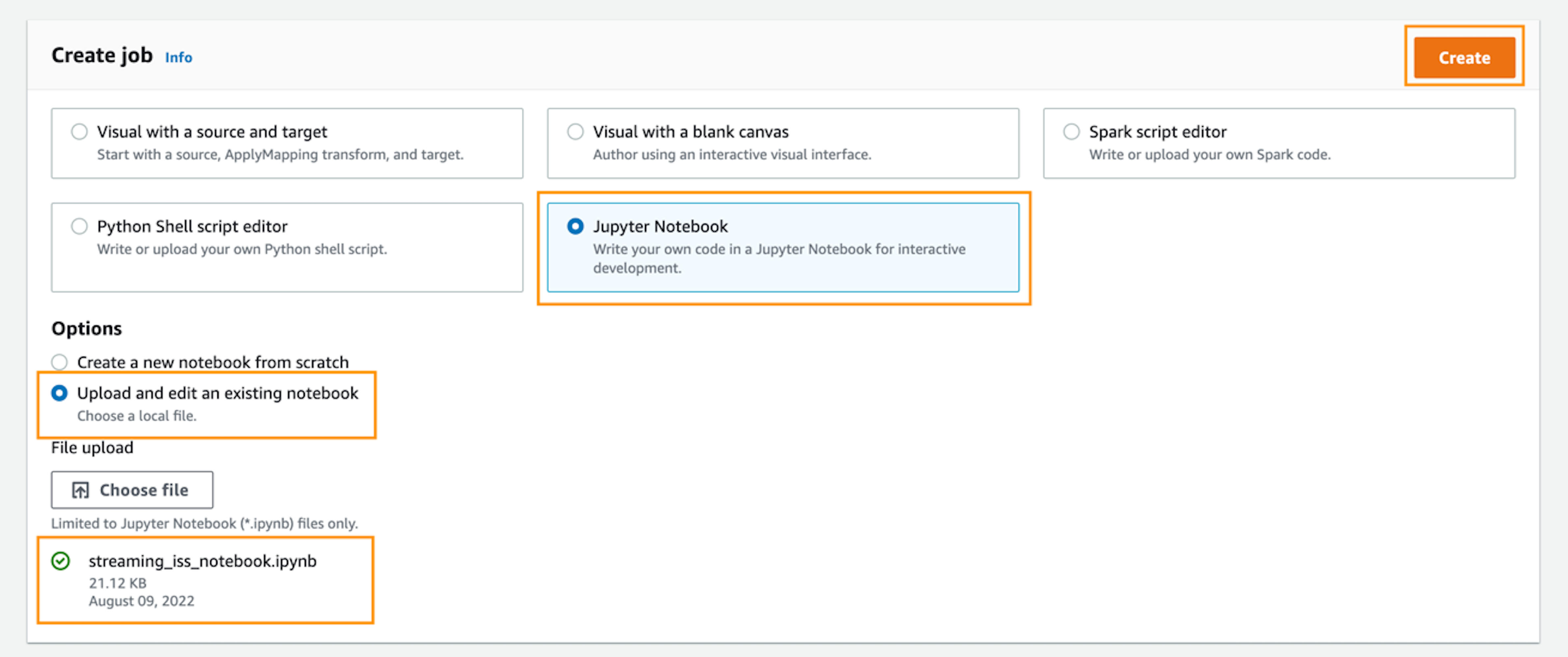
  3. Choose Create job.
  4. Select Jupyter Notebook.
  5. Under Options, select Upload and edit an existing notebook.
  6. Choose Choose file and browse to the notebook file you downloaded.
  7. Choose Create.
BDB-2464 Create Job
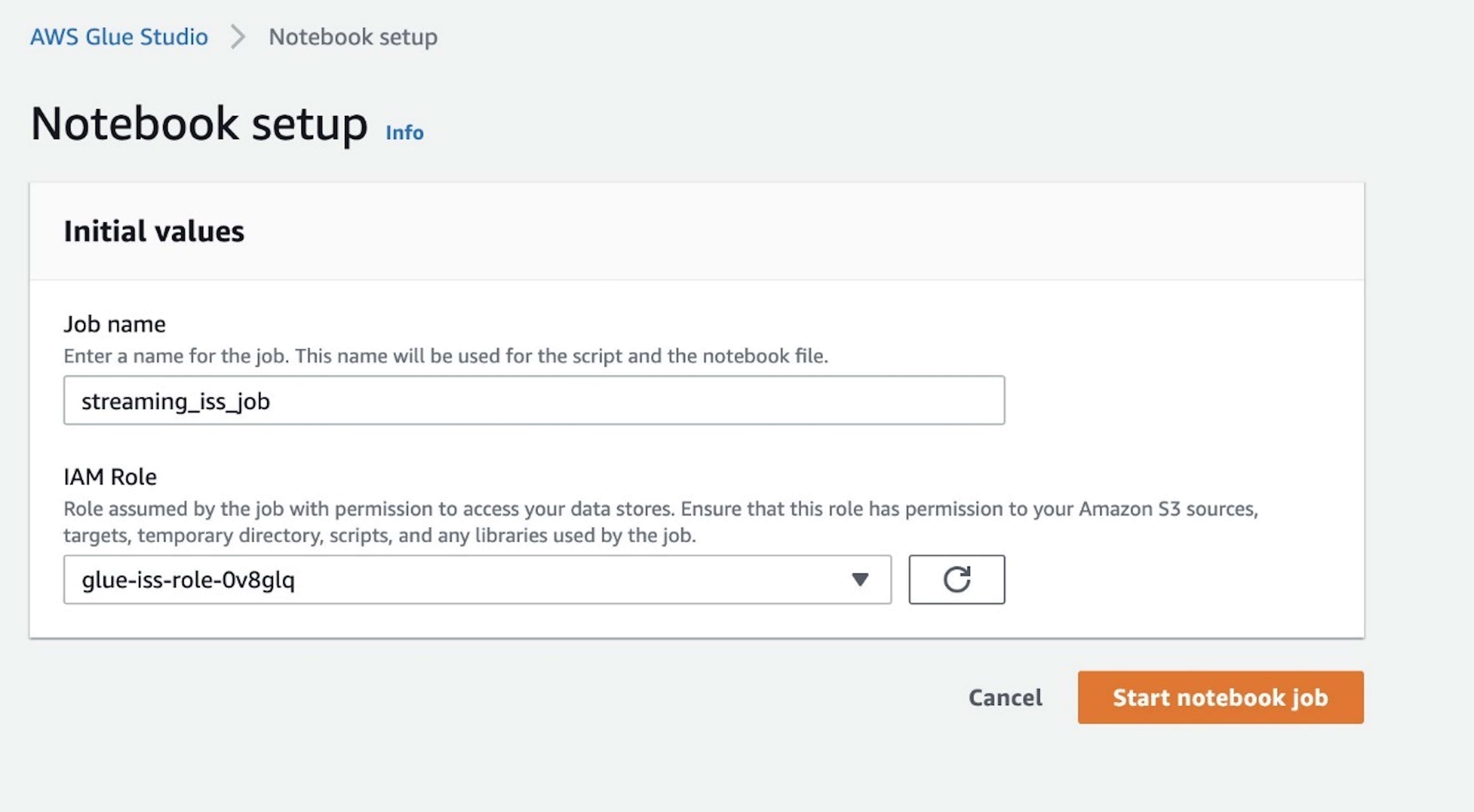
  1. For Job name¸ enter a name for the job.
  2. For IAM Role, use the role glue-iss-role-0v8glq, which is provisioned as part of the CloudFormation template.
  3. Choose Start notebook job.
BDB-2464 Start Notebook

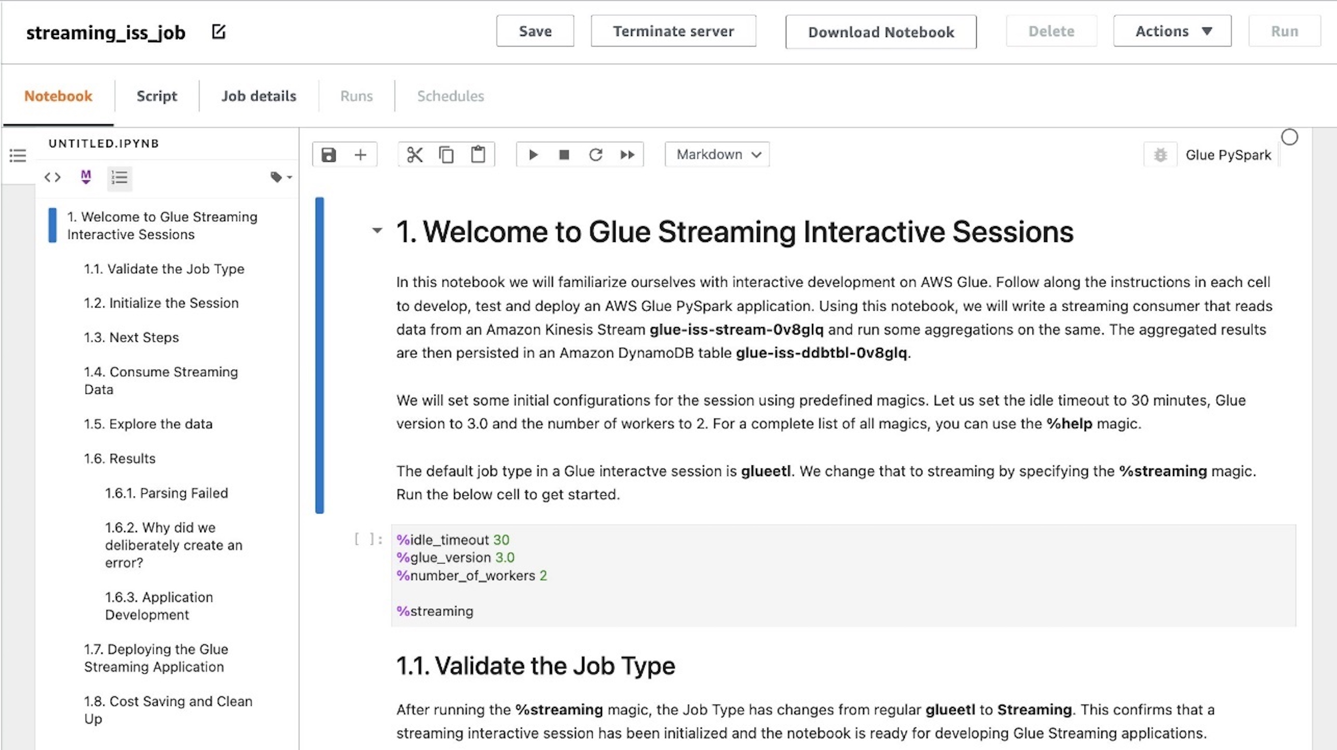
You can see that the notebook is loaded into the UI. There are markdown cells with instructions as well as code blocks that you can run sequentially. You can either run the instructions on the notebook or follow along with this post to continue with the job development.

BDB-2464 Explore Notebook

Run notebook cells

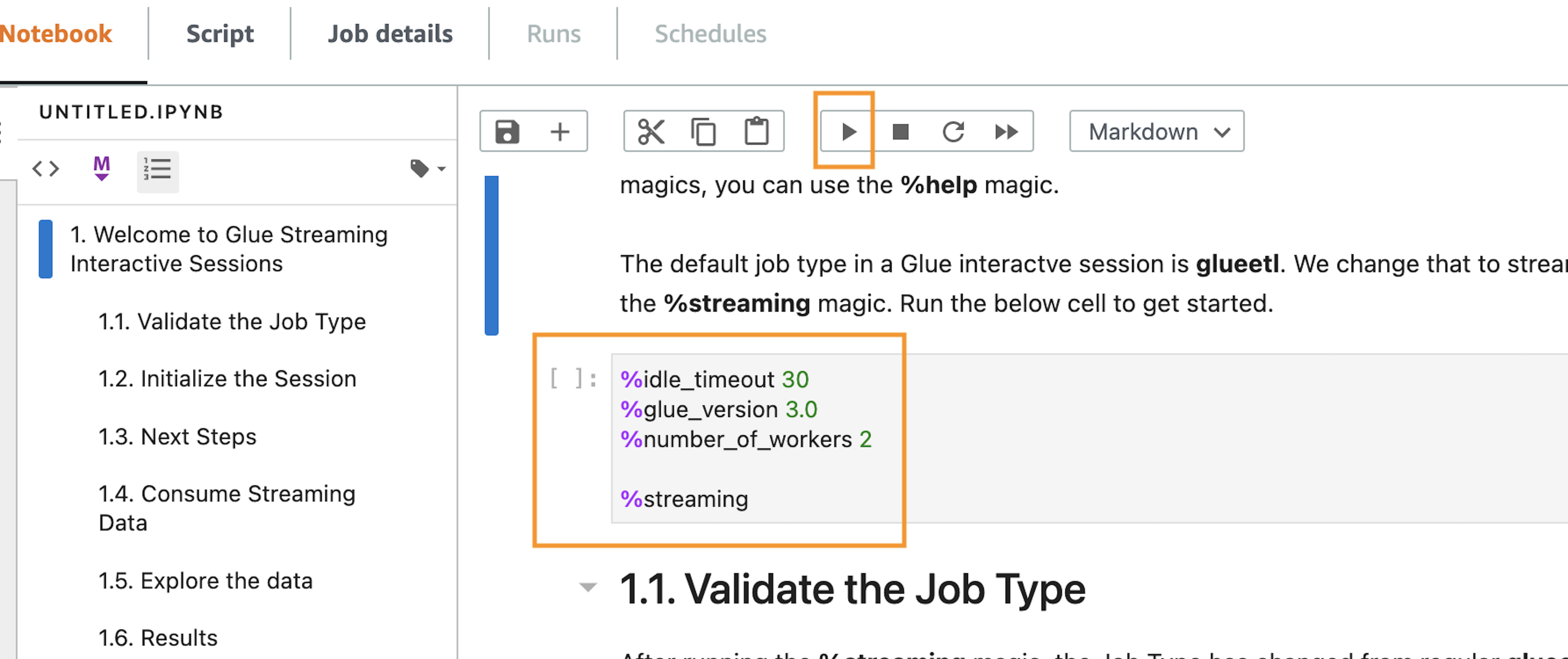
Let’s run the code block that has the magics. The notebook has notes on what each magic does.

  1. Run the first cell.
BDB-2464 Run First Cell

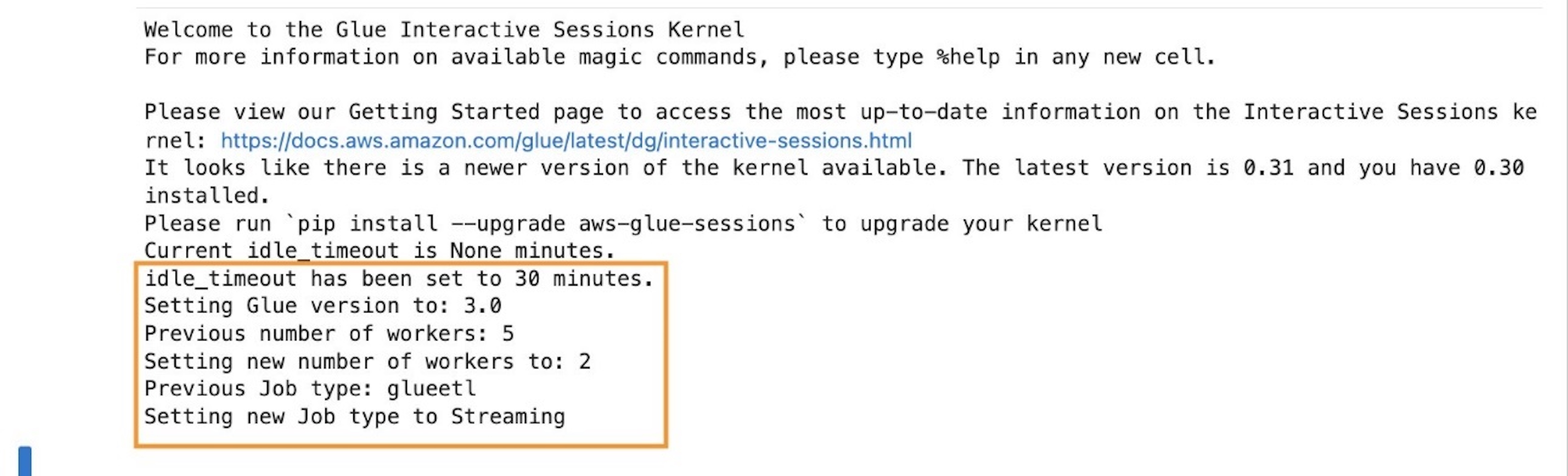
After running the cell, you can see in the output section that the defaults have been reconfigured.

BDB-2464 Configurations Set

In the context of streaming interactive sessions, an important configuration is job type, which is set to streaming. Additionally, to minimize costs, the number of workers is set to 2 (default 5), which is sufficient for our use case that deals with a low-volume simulated dataset.

Our next step is to initialize an AWS Glue streaming session.

  1. Run the next code cell.
BDB-2464 Initiate Session

After we run this cell, we can see that a session has been initialized and a session ID is created.

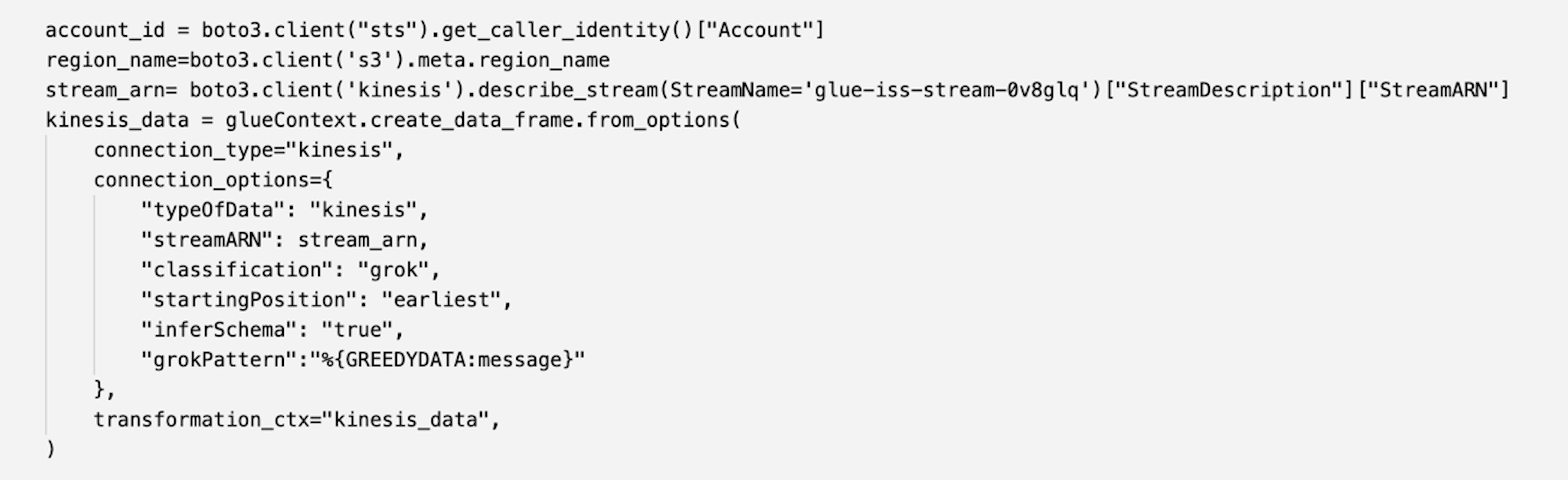
A Kinesis data stream and AWS Glue data generator job that feeds into this stream have already been provisioned and triggered by the CloudFormation template. With the next cell, we consume this data as an Apache Spark DataFrame.

  1. Run the next cell.
BDB-2464 Fetch From Kinesis

Because there are no print statements, the cells don’t show any output. You can proceed to run the following cells.

Explore the data stream

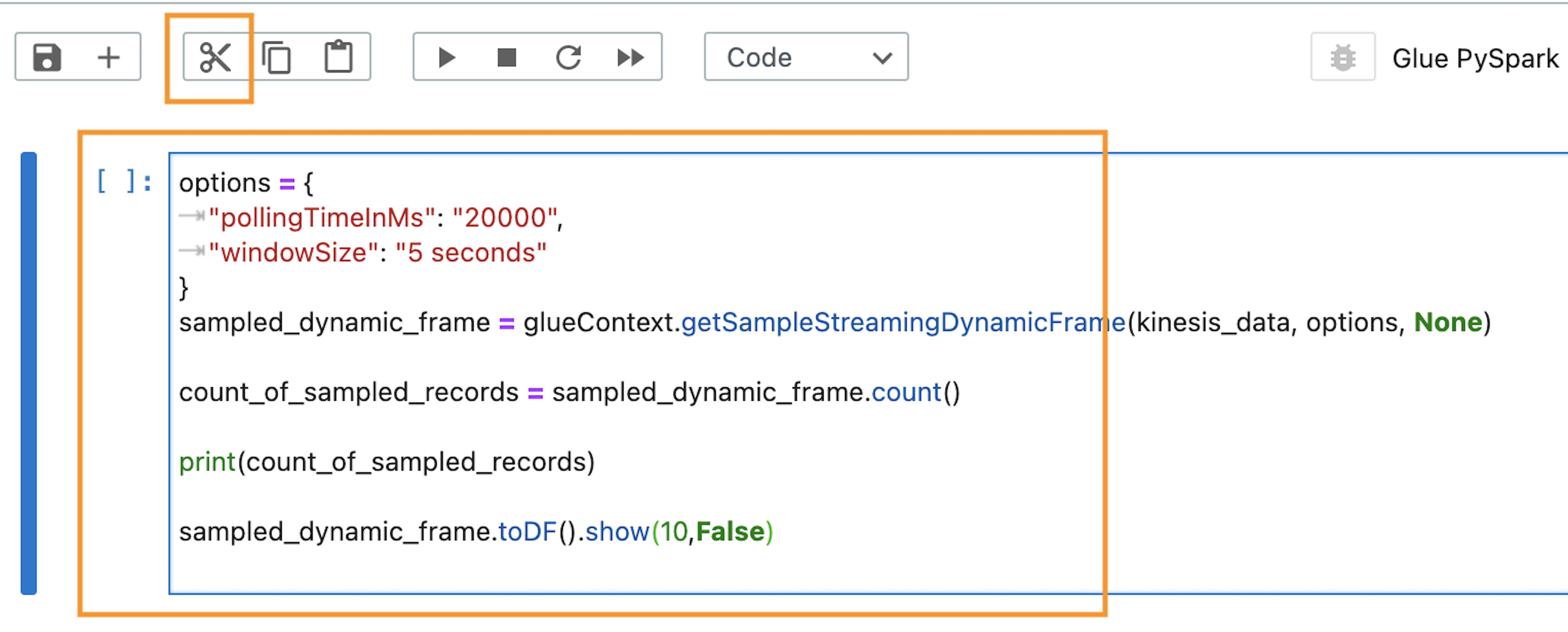
To help enhance the interactive experience in AWS Glue interactive sessions, GlueContext provides the method getSampleStreamingDynamicFrame. It provides a snapshot of the stream in a static DynamicFrame. It takes three arguments:

  • The Spark streaming DataFrame
  • An options map
  • A writeStreamFunction to apply a function to every sampled record

Available options are as follows:

  • windowSize – Also known as the micro-batch duration, this parameter determines how long a streaming query will wait after the previous batch was triggered.
  • pollingTimeInMs – This is the total length of time the method will run. It starts at least one micro-batch to obtain sample records from the input stream. The time unit is milliseconds, and the value should be greater than the windowSize.
  • recordPollingLimit – This is defaulted to 100, and helps you set an upper bound on the number of records that is retrieved from the stream.

Run the next code cell and explore the output.

BDB-2464 Sample Data

We see that the sample consists of 100 records (the default record limit), and we have successfully displayed the first 10 records from the sample.

Work with the data

Now that we know what our data looks like, we can write the logic to clean and format it for our analytics.

Run the code cell containing the reformat function.

Note that Python UDFs aren’t the recommended way to handle data transformations in a Spark application. We use reformat() to exemplify troubleshooting. When working with a real-world production application, we recommend using native APIs wherever possible.

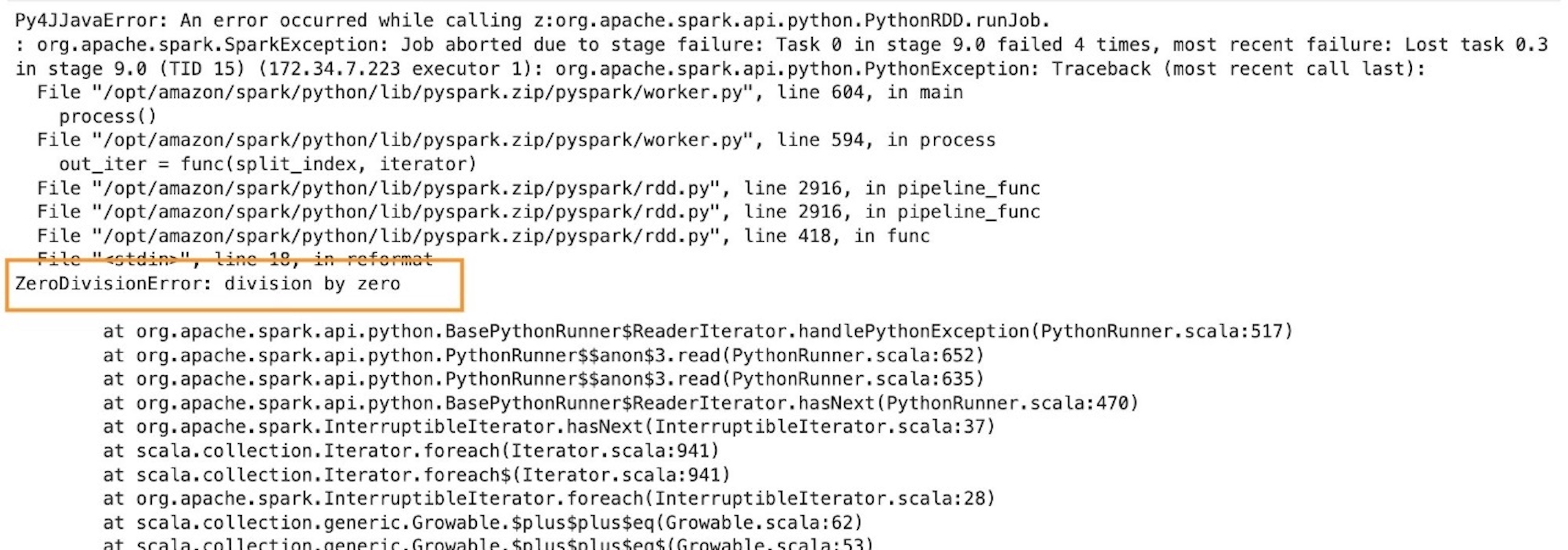
BDB-2464 Run The UDF

We see that the code cell failed to run. The failure was on purpose. We deliberately created a division by zero exception in our parser.

BDB-2464 Error Running The Code

Failure and recovery

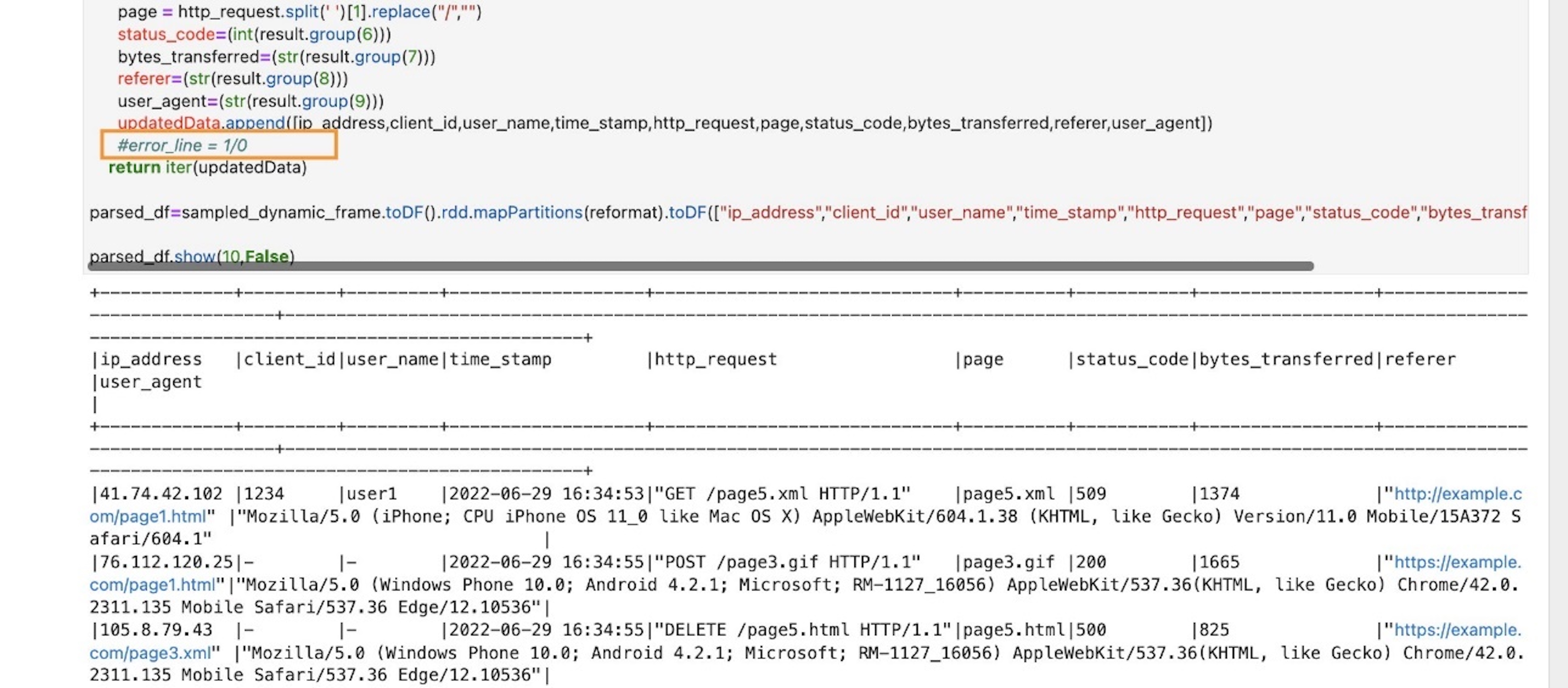
In case of a regular AWS Glue job, for any error, the whole application exits, and you have to make code changes and resubmit the application. However, in case of interactive sessions, the coding context and definitions are fully preserved and the session is still operational. There is no need to bootstrap a new cluster and rerun all the preceding transformation. This allows you to focus on quickly iterating your batch function implementation to obtain the desired outcome. You can fix the defects and run them in a matter of seconds.

To test this out, go back to the code and comment or delete the erroneous line error_line=1/0 and rerun the cell.

BDB-2464 Error Corrected

Implement business logic

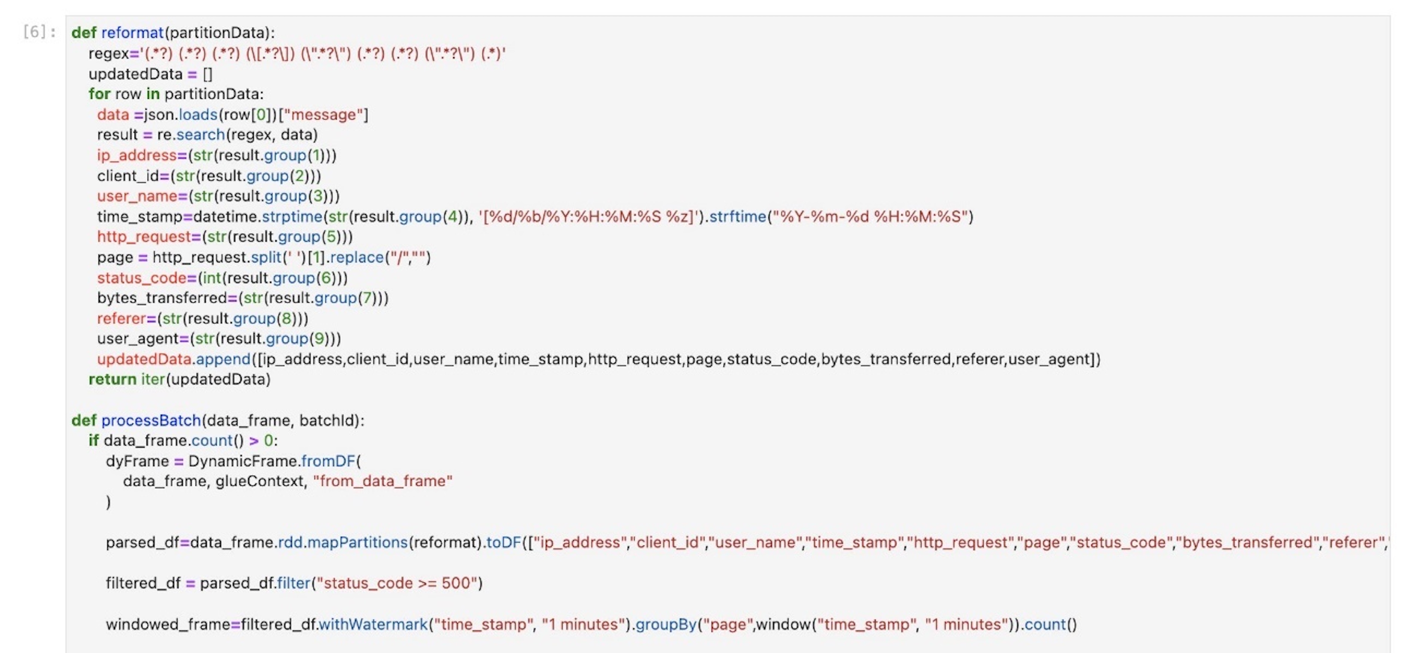
Now that we have successfully tested our parsing logic on the sample stream, let’s implement the actual business logic. The logics are implemented in the processBatch method within the next code cell. In this method, we do the following:

  • Pass the streaming DataFrame in micro-batches
  • Parse the input stream
  • Filter messages with status code >=500
  • Over a 1-minute interval, get the count of failures per webpage
  • Persist the preceding metric to a DynamoDB table (glue-iss-ddbtbl-0v8glq)
  1. Run the next code cell to trigger the stream processing.
BDB-2464 Trigger DDB Write
  1. Wait a few minutes for the cell to complete.
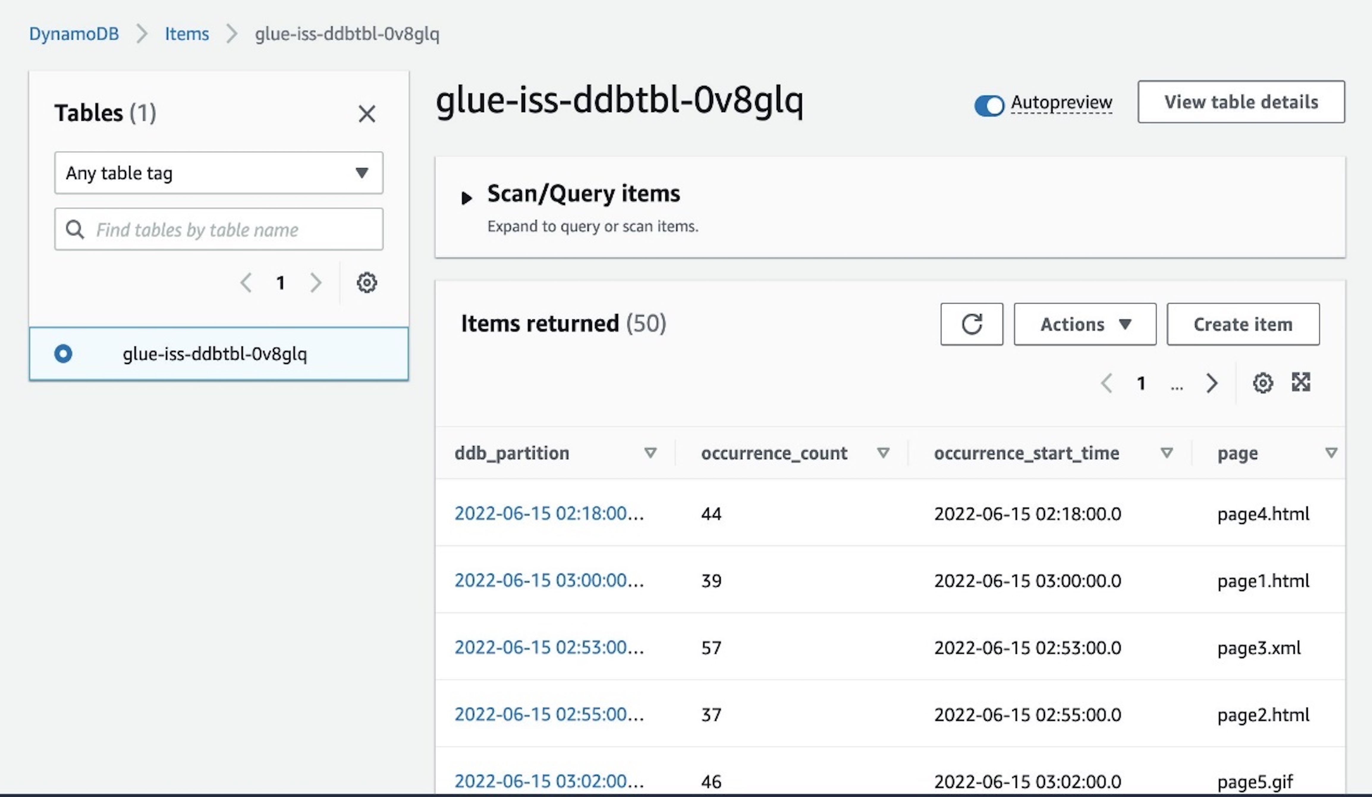
  2. On the DynamoDB console, navigate to the Items page and select the glue-iss-ddbtbl-0v8glq table.
BDB-2464 Explore DDB

The page displays the aggregated results that have been written by our interactive session job.

Deploy the streaming job

So far, we have been developing and testing our application using the streaming interactive sessions. Now that we’re confident of the job, let’s convert this into an AWS Glue job. We have seen that the majority of code cells are doing exploratory analysis and sampling, and aren’t required to be a part of the main job.

A commented code cell that represents the whole application is provided to you. You can uncomment the cell and delete all other cells. Another option would be to not use the commented cell, but delete just the two cells from the notebook that do the sampling or debugging and print statements.

To delete a cell, choose the cell and then choose the delete icon.

BDB-2464 Delete a Cell

Now that you have the final application code ready, save and deploy the AWS Glue job by choosing Save.

BDB-2464 Save Job

A banner message appears when the job is updated.

BDB-2464 Save Job Banner

Explore the AWS Glue job

After you save the notebook, you should be able to access the job like any regular AWS Glue job on the Jobs page of the AWS Glue console.

BDB-2464 Job Page

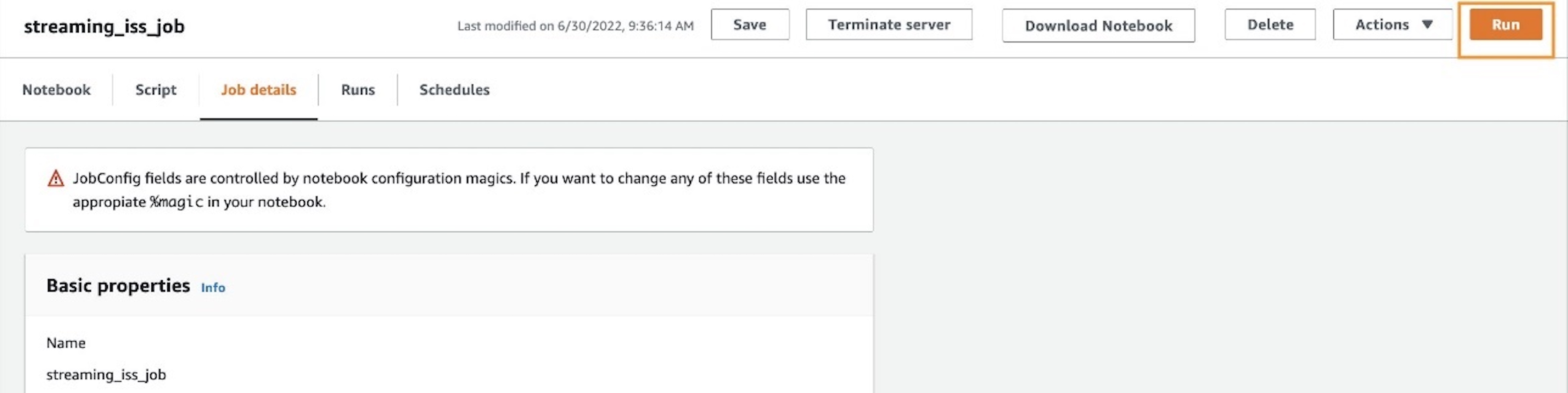
Additionally, you can look at the Job details tab to confirm the initial configurations, such as number of workers, have taken effect after deploying the job.

BDB-2464 Job Details Page

Run the AWS Glue job

If needed, you can choose Run to run the job as an AWS Glue streaming job.

BDB-2464 Job Run

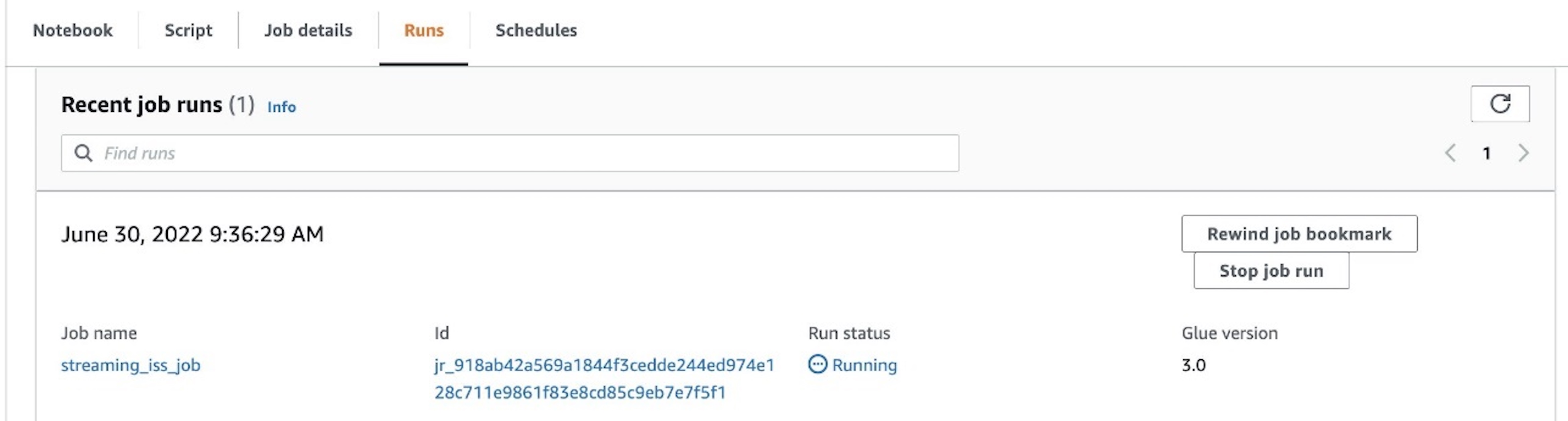
To track progress, you can access the run details on the Runs tab.

BDB-2464 Job Run Details

Clean up

To avoid incurring additional charges to your account, stop the streaming job that you started as part of the instructions. Also, on the AWS CloudFormation console, select the stack that you provisioned and delete it.

Conclusion

In this post, we demonstrated how to do the following:

  • Author a job using notebooks
  • Preview incoming data streams
  • Code and fix issues without having to publish AWS Glue jobs
  • Review the end-to-end working code, remove any debugging, and print statements or cells from the notebook
  • Publish the code as an AWS Glue job

We did all of this via a notebook interface.

With these improvements in the overall development timelines of AWS Glue jobs, it’s easier to author jobs using the streaming interactive sessions. We encourage you to use the prescribed use case, CloudFormation stack, and notebook to jumpstart your individual use cases to adopt AWS Glue streaming workloads.

The goal of this post was to give you hands-on experience working with AWS Glue streaming and interactive sessions. When onboarding a productionized workload onto your AWS environment, based on the data sensitivity and security requirements, ensure you implement and enforce tighter security controls.


About the authors

Arun A K is a Big Data Solutions Architect with AWS. He works with customers to provide architectural guidance for running analytics solutions on the cloud. In his free time, Arun loves to enjoy quality time with his family.
Linan Zheng is a Software Development Engineer at AWS Glue Streaming Team, helping building the serverless data platform. His works involve large scale optimization engine for transactional data formats and streaming interactive sessions.

Roman Gavrilov is an Engineering Manager at AWS Glue. He has over a decade of experience building scalable Big Data and Event-Driven solutions. His team works on Glue Streaming ETL to allow near real time data preparation and enrichment for machine learning and analytics.

Shiv Narayanan is a Senior Technical Product Manager on the AWS Glue team. He works with AWS customers across the globe to strategize, build, develop, and deploy modern data platforms.

How to automate updates for your domain list in Route 53 Resolver DNS Firewall

Post Syndicated from Guillaume Neau original https://aws.amazon.com/blogs/security/how-to-automate-updates-for-your-domain-list-in-route-53-resolver-dns-firewall/

Note: This post includes links to third-party websites. AWS is not responsible for the content on those websites.


Following the release of Amazon Route 53 Resolver DNS Firewall, Amazon Web Services (AWS) published several blog posts to help you protect your Amazon Virtual Private Cloud (Amazon VPC) DNS resolution, including How to Get Started with Amazon Route 53 Resolver DNS Firewall for Amazon VPC and Secure your Amazon VPC DNS resolution with Amazon Route 53 Resolver DNS Firewall. Route 53 Resolver DNS Firewall provides managed domain lists that are fully maintained and kept up-to-date by AWS and that directly benefit from the threat intelligence that we gather, but you might want to create or import your own list to have full control over the DNS filtering.

In this blog post, you will find a solution to automate the management of your domain list by using AWS Lambda, Amazon EventBridge, and Amazon Simple Storage Service (Amazon S3). The solution in this post uses, as an example, the URLhaus open Response Policy Zone (RPZ) list, which generates a new file every five minutes.

Architecture overview

The solution is made of the following four components, as shown in Figure 1.

  1. An EventBridge scheduled rule to invoke the Lambda function on a schedule.
  2. A Lambda function that uses the AWS SDK to perform the automation logic.
  3. An S3 bucket to temporarily store the list of domains retrieved.
  4. Amazon Route 53 Resolver DNS Firewall.
    Figure 1: Architecture overview

    Figure 1: Architecture overview

After the solution is deployed, it works as follows:

  1. The scheduled rule invokes the Lambda function every 5 minutes to fetch the latest domain list available.
  2. The Lambda function fetches the list from URLhaus, parses the data retrieved, formats the data, uploads the list of domains into the S3 bucket, and invokes the Route 53 Resolver DNS Firewall importFirewallDomains API action.
  3. The domain list is then updated.

Implementation steps

As a first step, create your own domain list on the Route 53 Resolver DNS Firewall. Having your own domain list allows you to have full control of the list of domains to which you want to apply actions, as defined within rule groups.

To create your own domain list

  1. In the Route 53 console, in the left menu, choose Domain lists in the DNS firewall section.
  2. Choose the Add domain list button, enter a name for your owned domain list, and then enter a placeholder domain to initialize the domain list.
  3. Choose Add domain list to finalize the creation of the domain list.
    Figure 2: Expected view of the console

    Figure 2: Expected view of the console

The list from URLhaus contains more than a thousand records. You will use the ImportFirewallDomains endpoint to upload this list to DNS Firewall. The use of the ImportFirewallDomains endpoint requires that you first upload the list of domains and make the list available in an S3 bucket that is located in the same AWS Region as the owned domain list that you just created.

To create the S3 bucket

  1. In the S3 console, choose Create bucket.
  2. Under General configuration, configure the AWS Region option to be the same as the Region in which you created your domain list.
  3. Finalize the configuration of your S3 bucket, and then choose Create bucket.

Because a new file is created every five minutes, we recommend setting a lifecycle rule to automatically expire and delete files after 24 hours to optimize for cost and only save the most recent lists.

To create the Lambda function

  1. Follow the steps in the topic Creating an execution role in the IAM console to create an execution role. After step 4, when you configure permissions, choose Create Policy, and then create and add an IAM policy similar to the following example. This policy needs to:
    • Allow the Lambda function to put logs in Amazon CloudWatch.
    • Allow the Lambda function to have read and write access to objects placed in the created S3 bucket.
    • Allow the Lambda function to update the firewall domain list.
    • {
          "Version": "2012-10-17",
          "Statement": [
              {
                  "Action": [
                      "logs:CreateLogGroup",
                      "logs:CreateLogStream",
                      "logs:PutLogEvents"
                  ],
                  "Resource": "arn:aws:logs:<region>:<accountId>:*",
                  "Effect": "Allow"
              },
              {
                  "Action": [
                      "s3:PutObject",
                      "s3:GetObject"
                  ],
                  "Resource": "arn:aws:s3:::<DNSFW-BUCKET-NAME>/*",
                  "Effect": "Allow"
              },
              {
                  "Action": [
                      "route53resolver:ImportFirewallDomains"
                  ],
                  "Resource": "arn:aws:route53resolver:<region>:<accountId>:firewall-domain-list/<domain-list-id>",
                  "Effect": "Allow"
              }
          ]
      }

  2. (Optional) If you decide to use the example provided by AWS:
    • After cloning the repository: Build the layer following the instruction included in the readme.md and the provided script.
    • Zip the lambda.
    • In the left menu, select Layers then Create Layer. Enter a name for the layer, then select Upload a .zip file. Choose to upload the layer (node-axios-layer.zip).
    • As a compatible runtime, select: Node.js 16.x.
    • Select Create
  3. In the Lambda console, in the same Region as your domain list, choose Create function, and then do the following:
    • Choose your desired runtime and architecture.
    • (Optional) To use the code provided by AWS: Select Node.js 16.x as the runtime.
    • Choose Change the default execution role.
    • Choose Use an existing role, and then pick the role that you just created.
  4. After the Lambda function is created, in the left menu of the Lambda console, choose Functions, and then select the function you created.
    • For Code source, you can either enter the code of the Lambda function or choose the Upload from button and then choose the source for the code. AWS provides an example of functioning code on GitHub under a MIT-0 license.

    (optional) To use the code provided by AWS:

    • Choose the Upload from button and upload the zipped code example.
    • After the code is uploaded, edit the default Runtime settings: Choose the Edit button and set the handler to be equal to: LambdaRpz.handler
    • Edit the default Layers configuration, choose the Add a layer button, select Specify an ARN and enter the ARN of the layer created during the optional step 2.
    • Edit the environment variables of the function: Select the Edit button and define the three following variables:
      1. Key : FirewallDomainListId | Value : <domain-list-id>
      2. Key : region | Value : <region>
      3. Key : s3Prefix | Value : <DNSFW-BUCKET-NAME>

The code that you place in the function will be able to fetch the list from URLhaus, upload the list as a file to S3, and start the import of domains.

For the Lambda function to be invoked every 5 minutes, next you will create a scheduled rule with Amazon EventBridge.

To automate the invoking of the Lambda function

  1. In the EventBridge console, in the same AWS Region as your domain list, choose Create rule.
  2. For Rule type, choose Schedule.
  3. For Schedule pattern, select the option A schedule that runs at a regular rate, such as every 10 minutes, and under Rate expression set a rate of 5 minutes.
    Figure 3: Console view when configuring a schedule

    Figure 3: Console view when configuring a schedule

  4. To select the target, choose AWS service, choose Lambda function, and then select the function that you previously created.

After the solution is deployed, your domain list will be updated every 5 minutes and look like the view in Figure 4.

Figure 4: Console view of the created domain list after it has been updated by the Lambda function

Figure 4: Console view of the created domain list after it has been updated by the Lambda function

Code samples

You can use the samples in the amazon-route-53-resolver-firewall-automation-examples-2 GitHub repository to ease the automation of your domain list, and the associated updates. The repository contains script files to help you with the deployment process of the AWS CloudFormation template. Note that you need to have the AWS Command Line Interface (AWS CLI) installed and properly configured in order to use the files.

To deploy the CloudFormation stack

  1. If you haven’t done so already, create an S3 bucket to store the artifacts in the Region where you wish to deploy. This name of this bucket will then be referenced as ParamS3ArtifactBucket with a value of <DOC-EXAMPLE-BUCKET-ARTIFACT>
  2. Clone the repository locally.
    git clone https://github.com/aws-samples/amazon-route-53-resolver-firewall-automation-examples-2
  3. Build the Lambda function layer. From the /layer folder, use the provided script.
    . ./build-layer.sh
  4. Zip and upload the artifact to the bucket created in step 1. From the root folder, use the provided script.
    . ./zipupload.sh <ParamS3ArtifactBucket>
  5. Deploy the AWS CloudFormation stack by using either the AWS CLI or the CloudFormation console.
    • To deploy by using the AWS CLI, from the root folder, type the following command, making sure to replace <region>, <DOC-EXAMPLE-BUCKET-ARTIFACT>, <DNSFW-BUCKET-NAME>, and <DomainListName>with your own values.
      aws --region <region> cloudformation create-stack --stack-name DNSFWStack --capabilities CAPABILITY_NAMED_IAM --template-body file://./DNSFWStack.cfn.yaml --parameters ParameterKey=ParamS3ArtifactBucket,ParameterValue=<DOC-EXAMPLE-BUCKET-ARTIFACT> ParameterKey=ParamS3RpzBucket,ParameterValue=<DNSFW-BUCKET-NAME> ParameterKey=ParamFirewallDomainListName,ParameterValue=<DomainListName>

    • To deploy by using the console, do the following:
      1. In the CloudFormation console, choose Create stack, and then choose With new resources (standard).
      2. On the creation screen, choose Template is ready, and upload the provided DNSFWStack.cfn.yaml file.
      3. Enter a stack name and configure the requested parameters with your desired configuration and outcomes. These parameters include the following:
        • The name of your firewall domain list.
        • The name of the S3 bucket that contains Lambda artifacts.
        • The name of the S3 bucket that will be created to contain the files with the domain information from URLhaus.
      4. Acknowledge that the template requires IAM permission because it will create the role for the Lambda function and manage its IAM policy, and then choose Create stack.

After a few minutes, all the resources should be created and the CloudFormation stack is now deployed. After 5 minutes, your domain list should be updated, as shown in Figure 5.

Figure 5: Console view of CloudFormation after the stack has been deployed

Figure 5: Console view of CloudFormation after the stack has been deployed

Conclusions and cost

In this blog post, you learned about creating and automating the update of a domain list that you fully control. To go further, you can extend and replicate the architecture pattern to fetch domain names from other sources by editing the source code of the Lambda function.

After the solution is in place, in order for the filtering to be effective, you need to create a rule group referencing the domain list and associate the rule group with some of your VPCs.

For cost information, see the AWS Pricing Calculator. This solution will be invoked 60 (minutes) * 24 (hours) * 30 (days) / 5 (minutes) = 8,640 times per month, invoking the Lambda function that will run for an average of 400 minutes, storing an average of 0.5 GB in Amazon S3, and creating a domain list that averages 1,500 domains. According to our public pricing, and without factoring in the AWS Free Tier, this will incur the estimated total cost of $1.43 per month for the filtering of 1 million DNS requests.

 
If you have feedback about this post, submit comments in the Comments section below. If you have questions about this post, contact AWS Support.

Want more AWS Security news? Follow us on Twitter.

Guillaume Neau

Guillaume Neau

Guillaume is a solutions architect of France with an expertise in information security that focus on building solutions that improve the life of citizens.

Packing Up and Backing Up: It’s Time for School

Post Syndicated from Josephine Quock original https://www.backblaze.com/blog/packing-up-and-backing-up-its-time-for-school/

Note from the Editor: When students head off to college, they take their data and computers with them. We wanted to dig into what students and other young tech users are doing to save and protect their data, so we invited our intern, Josephine, to develop some resources for you before she heads off to college.

Apart from discovering the outside world and learning more about who you are as a person, the university experience is, at its core, about the pursuit of knowledge. In years past, students would store that knowledge in spiral-bound notebooks or scattered sheets of loose leaf, but today it’s all digital. While there’s no doubt that computers have changed everything from how we research to how assignments are turned in, technology comes with its own set of challenges. I wondered: how much are students taught about how to keep their data safe? My experience at Backblaze has taught me a lot about the importance of backing up your data, and I want to share that with other college students.

Lesson One: Syncing is Not Backing Up

If students do think about how to preserve their data, most are content to let services like iCloud or OneDrive handle it. What they may not realize (and I didn’t) is that these sync services are completely different from a true backup. Before interning at Backblaze, I didn’t even think about backing up, let alone understand the importance of it or the best strategies to back up my data. I couldn’t tell you the difference between backup and sync services. Because my photos and contacts were synced on my iPhone, iPad, and even my MacBook, I assumed all this data was saved and in good hands. However, working at Backblaze taught me the importance of backing up to prevent losing my data.

For example, if I were to delete a photo on my iPhone, syncing means that it would also delete on my other devices. Backing up gives you an additional copy of the data that doesn’t follow the same rules as your syncing services. If I accidentally delete something or get a virus, a backup with version history means that I could restore an earlier version of my files or library. This is why ensuring the safety of your data is proactive, as backing up can provide security in the event of hardware failure, cyber attack, natural disaster, or even a careless mistake.

Lesson Two: You Might Need Your Old Data

Let me provide an example that we college students have experienced at least once throughout our time in university: the frustration and annoyance of endlessly searching through the deepest corners of our devices to find an important document, only to not find it in the end.

A few months ago, I was given the option to select a prompt for an essay of my choosing from a couple of short stories. “The Tell-Tale Heart” by Edgar Allen Poe immediately caught my eye because I had read it and written a paper on it in high school. I enjoyed the story in high school and liked the idea of comparing my new paper with my old to see how much I’d grown as a writer. I browsed and inspected every possible drive on multiple email accounts—no luck.

Looking back, I wished that I had saved all the files and emails from middle and high school. But since I didn’t, I wasn’t able to review what I had written and couldn’t see the progress and improvement in my writing. Had I backed up all the data of my high school years, I could have read my essay on “The Tell-Tale Heart” and expanded on my original ideas. I was warned many times that all my documents from my account would be deleted. I knew this information and yet I still didn’t do anything about it.

Lesson Three: There Are Easy Answers

As a college student, I need a backup service that’s easy to use and affordable. Since Backblaze first started offering consumer backup, they’ve prioritized both of those things. According to an internal Backblaze’s Customer Survey in 2022, users love using the service because of the price, unlimited data backup, and most importantly ease of use. Backups are automatic, and 45% of Backblaze users spend less than $100 per year on all their backup services (including Backblaze).

Now that I will be going into my fourth year in college, I will have other important documents beyond my school work since I am going to be applying for more internships and jobs when I graduate. My resume, job applications, school projects, and essays are all things that I can’t risk losing. Additionally, lots of my photos are saved to social media accounts, and I want to save them somewhere besides my phone or on those platforms.

Lesson Learned!

After college, I plan on purchasing a new computer and will need to back everything up on my current computer to transfer over to my new laptop. Not only will that make sure that I don’t lose data when I change devices, but (rather than buying an external drive that I need to keep track of) I can use my Backblaze account. I will be using multiple devices to access my single Backblaze account. Once I have my new laptop, I just have to log in from my new device and restore all my files. I won’t have to worry about losing an external hard drive or making sure the files on a hard drive are updated.

With school back in session and the end of my university experience approaching, my social media, school work, and job search exist on all my devices. I can’t imagine losing any of it. After interning at Backblaze and hearing so many disaster stories, I will definitely be backing up my data, and I recommend that other students do too. That’s why services like Backblaze are really helpful.

The post Packing Up and Backing Up: It’s Time for School appeared first on Backblaze Blog | Cloud Storage & Cloud Backup.

Announcing new AWS IAM Identity Center APIs to manage users and groups at scale

Post Syndicated from Sharanya Ramakrishnan original https://aws.amazon.com/blogs/security/announcing-new-aws-iam-identity-center-apis-to-manage-users-and-groups-at-scale/

If you use AWS IAM Identity Center (successor to AWS Single Sign-On) as your identity source, you create and manage your users and groups manually in the IAM Identity Center console. However, you may prefer to automate this process to save time, spend less administrative effort, and to scale effectively as your organization grows. If you use IAM Identity Center with a supported identity provider (IdP) or Microsoft Active Directory (AD), you may want to check if the right users and groups have synced into IAM Identity Center. You can do this manually, but now you can use the new APIs to make the process easier by setting up automated checks that query this information from IAM Identity Center and notify you only when you need to intervene.

This post explains how you can use IAM Identity Center APIs to automate managing users and groups in a scalable manner and gain better visibility into users and groups in the Identity Center directory. These automations can help you save time and reduce administrative effort. We will provide some background on how IAM Identity Center works and how you can use the new APIs to help simplify your workflows.

Background

IAM Identity Center allows you to centrally manage access to all of your AWS accounts within AWS Organizations or your applications. Using IAM Identity Center is the AWS recommendation for managing the workforce identities of the human users in your organization who access AWS resources. It provides you with the flexibility to create and manage users and groups in the Identity Center directory, or bring in your users and groups from a different identity source such as Active Directory or an external identity provider (IdP). After IAM Identity Center is configured, you can look up users or groups to grant them single sign-on access to AWS accounts, applications, or both. By signing-in once in the IAM Identity Center portal, your users can access their assigned AWS accounts, as well as Identity Center enabled applications such as Amazon SageMaker Studio or Amazon EMR Studio, as well as cloud applications such as Jira, Salesforce, and Tableau.

While IAM Identity Center simplifies user access, you may prefer to manage these users and groups at scale, and audit their access regularly to meet your security requirements. You may also want to automate the process of giving users access to AWS and the resources they need to do their job. Previously, you could only manage identities in the Identity Center directory manually by using the IAM Identity Center console. Now, you can use the new Identity Center APIs to build automation that manages the Identity Center directory users and groups for you.

With these Identity Center APIs, you can build automated workflows to do the following tasks:

  • Provision and de-provision users and groups.
  • Add new members to a group or remove them from a group.
  • Query information about users and groups in the Identity Center directory.
  • Update information about users and groups.
  • Find out which users are members of which groups.

You can create automated workflows using the APIs to define who has access to AWS accounts or applications through IAM Identity Center, and provide them with the right resources to do their job. Automating workflows can save you time and can reduce your administrative effort. With the new APIs, you can auto-generate reports about users and their IAM Identity Center access configurations. These automated reports can provide you with greater visibility to evaluate your security posture.

Provision, manage, and de-provision users and groups in IAM Identity Center

As your enterprise grows, you may want to automate your administrative tasks to reduce manual effort, save time, and scale efficiently. If you’re a cloud administrator or IT administrator who manages which employees in your organization need access to AWS as part of their job role, or what AWS resources they need so they can develop applications, now you can set up automated workflows that manage this for you.

Consider the following scenario. Your organization uses the Identity Center directory as the source for user information, and a new data scientist joins your company. You want them to be granted access to log in to AWS automatically based on their job role. After they log in, you want them to have access to the AWS resources and applications that you have approved for their job role, including Amazon SageMaker, AWS Managed Grafana, and multiple S3 buckets. Previously, you had to use the AWS Management Console to manually create a new user object and then add the new data scientist to the AWS_Data_Science group. With the new APIs, you can set up an automated workflow that creates a new user and adds the user to relevant groups in the Identity Center directory, as soon as the new data scientist is added to your human resources (HR) system.

A sample AWS Identity Store operations python script called identitystore_operations.py is available in the iam-identitycenter-identitystoreapi-operations GitHub repository. This sample program shows you how you can automate Identity Store operations to create a new user, add the user to a group, list group memberships, and update the user’s group memberships operations. This sample program requires the AWS SDK for Python (Boto3). For instructions to install the AWS SDK for Python, see the Boto3 Quickstart.

The following is an example to see all supported operations available in the sample script.

python identitystore_operations.py —h

The following is example output:

usage: identitystore_operations.py [-h]
{create_user,create_group,adduser_to_group,delete_group,list_members,list_membership}
...
positional arguments:
{create_user,create_group,adduser_to_group,delete_group,list_members,list_membership}

options:
-h, --help show this help message and exit

Next is an example of how you can create the new user John Doe in the Identity Center directory and add the user to an existing AWS_Data_Science group.

python identitystore_operations.py create_user --identitystoreid d-123456a7890 --username johndoe --givenname John --familyname Doe --groupname AWS_Data_Science

The following is example output:

User:johndoe with UserId:12345678-9012-3456-789a-bcdef021345a created successfully
User:johndoe added to Group:AWS_Data_Science successfully

To continue with this example, consider a scenario where the data scientist transitions to a role as an applied scientist, and needs access to additional AWS applications and resources. Rather than using the IAM Identity Center console to manually update the user’s information and add them to the AWS_Applied_Scientists group, you can now use automation to update the user and provide them with the access they need.

The following is an example of how the previously-created user johndoe can be added to the AWS_Applied_Scientists group.

python identitystore_operations.py adduser_to_group --identitystoreid d-123456a7890 --groupname AWS_Applied_Scientists --username johndoe

The following is example output:

User:johndoe added to Group:AWS_Applied_Scientists successfully

Finally for this scenario, consider that this employee leaves your company. Rather than using the IAM Identity Center console to manually delete their user object, now your automation can delete the user as soon as they are removed from your HR system.

Evaluate your security posture in IAM Identity Center

To maintain visibility across AWS, it is a best practice to regularly audit and evaluate the security controls for any service that you use. It’s also a best practice to identify the AWS accounts or applications that an employee can access. Having access to this information helps you maintain and improve your company’s security posture. As a cloud administrator, you may need to submit periodic reports to auditors enumerating the employees who have access to AWS. If you or your IT team manage users and groups in a different source system, you also need to track whether the right users and groups are synced into AWS.


The following is an example of how you can find the members of the AWS_Applied_Scientists group.

python identitystore_operations.py list_members --identitystoreid d-123456a7890 --groupname AWS_Applied_Scientists

The following is example output:

UserName:johndoe,Display Name: John Doe

For example, consider a scenario in which you use Active Directory as your identity source. You want to confirm that the right set of users and groups have been synced into the Identity Center directory. After the users and groups are confirmed, you are required to submit this list of users and groups with access to AWS to auditors every quarter. Rather than manually verifying which employees have access to AWS and manually creating a list for the auditors, now you can use the new APIs to create a workflow that automatically queries the users and groups in the Identity Center directory, compares it to your list of intended Active Directory users and groups who should have AWS access, and provides you the information about whether there are any users or groups who have access that was not intended. Additionally, you can set up a script to generate reports every quarter for the auditors.

The following is an example of how you can find the group memberships of the specific user johndoe.

python identitystore_operations.py list_membership --identitystoreid d-123456a7890 --username johndoe

The following is example output:

User :johndoe is a member of the following groups
AWS_Data_Science
AWS_Applied_Scientists

Conclusion

In this post, you learned how to use IAM Identity Center APIs to automate managing users and groups in a scalable manner and gain better visibility into users and groups in the Identity Center directory.

The IAM Identity Center APIs for user and group management expand the capabilities of existing Identity Store APIs, helping you build scalable workflows. They help your IT and cloud teams save time and reduce administrative effort through automation.

To learn more about using IAM Identity Center or the user and group management APIs, see the AWS IAM Identity Center User Guide or the Identity Store API Reference Guide.

If you have feedback about this post, submit comments in the Comments section below. If you have questions about this post, start a new thread on AWS IAM Identity Center re:Post or contact AWS Support.

Want more AWS Security news? Follow us on Twitter.

Author

Sharanya Ramakrishnan

Sharanya is a Senior Technical Product Manager in the AWS Identity team. She enjoys solving customer problems through meaningful products, particularly in the dynamic security and identity space. Outside of work, Sharanya likes to travel and enjoys hiking and reading.

Author

Siva Rajamani

Siva is a Boston-based Enterprise Solutions Architect. He enjoys working closely with customers and supporting their digital transformation and AWS adoption journey. His core areas of focus are Serverless, Application Integration, and Security.

Bala KP

Bala KP

Bala KP is a Sr Partner Solutions Architect at Amazon Web Services. He helps global system integrator partners and customers in the financial services and insurance domain to move their most sensitive workloads to AWS.
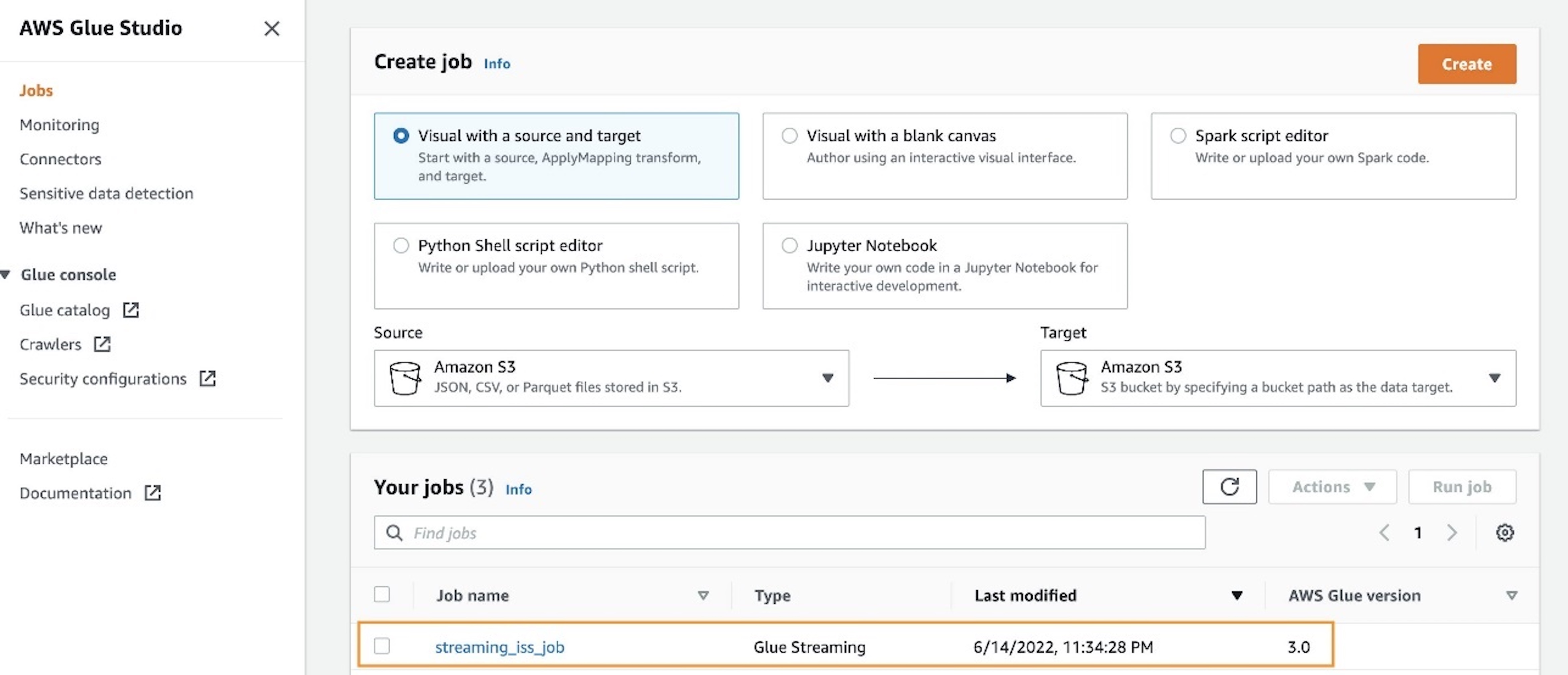
[$] A framework for code tagging

Post Syndicated from original https://lwn.net/Articles/906660/

Kernel code can, at times, be quite inward looking; it often refers to
itself. To enable this introspection, the kernel has evolved several
mechanisms for identifying specific locations in the code and carrying out
actions related to those locations. The code-tagging
framework
patch set, posted by Suren Baghdasaryan and Kent Overstreet,
is an attempt to replace various ad hoc implementations with a
single framework, and to add some new applications as well.

25 Years of Nmap: Happy Scan-iversary!

Post Syndicated from Tod Beardsley original https://blog.rapid7.com/2022/09/01/25-years-of-nmap-happy-scan-iversary/

25 Years of Nmap: Happy Scan-iversary!

I didn’t know it then, but on September 1, 1997, my life changed. That was the day that Fyodor’s Nmap was first released to the world, courtesy of the venerable Phrack magazine. (By the way, check out our recent podcast with Fyodor himself if you haven’t yet.) At the time, I had just started my legitimate IT career, but boy oh boy, I was in the thick of it when it came to hackery hijinks. I won’t admit to any crimes or anything in this, my now-very-legitimate company’s blog post, but let me tell you: 1997 was a truly magical time for the nascent field of what would eventually become known as information security.

At the risk of making this sound like a “kids-these-days/back-in-my-day” kind of blog post, let me just say that if you wanted to probe and profile computers — yes, even computers you owned, legitimately — your choices were simultaneously limited and practically unbounded. In order to conduct network scanning, you had a bunch of tools available to you, all of which worked a little differently, ranging from “completely broken” to “kind of okay for some users.” People who were into this sort of thing generally got frustrated with the tooling floating around and wrote their own, which meant that their tools tended to only work for them, since these projects were heavily dependent on that one person’s local operating system configuration.

Nmap changed all that.

Early infosec’s magic moment

From the outset, Nmap was a simple tool that literally fit in a magazine article about network scanning tactics and tricks. It was two files of about 2,100 lines of code, and unlike many hacker tools of the day, it actually compiled for me on the first try.

Most importantly, Fyodor’s code style was weirdly easy to read, even for a non-programmer hacker hobbyist like myself (I didn’t get my first “real” IT job until 1998, but I did spend quite a bit of time in university computer labs for… reasons).

25 Years of Nmap: Happy Scan-iversary!
A snippet of the original code published in Phrack 51

Smack in the middle, you can see elements like `send_tcp_raw()` (pictured above) that directly reflected the language in the TCP/IP standard, RFC 793, so the code was generally accessible to both hobbyists and professionals who had motivation to figure out how this TCP/IP stuff worked, really.

Incidentally, other projects were also popping off at the time, as well — l0phtcrack (a proprietary utility for recovering passwords) was released a few months before, and Nessus (a little open-source vulnerability scanner) was released a few months after, so there was definitely something in the ether during this 12-month period. Hacker tooling was transforming into infosec tooling, which meant more “luser n00bs,” like myself, could get themselves enmeshed and enamored of the occult magicks of internet technology. Nmap, at least for me, stood out as a true oracle to the weird ways of packet crafting and network sleight-of-hand you could use in fun, unexpected ways to learn about the world.

Happy Scan-iversary, Nmap. Thanks for the cool career.

Additional reading:

NEVER MISS A BLOG

Get the latest stories, expertise, and news about security today.

Security updates for Thursday

Post Syndicated from original https://lwn.net/Articles/906778/

Security updates have been issued by Fedora (pdns-recursor, thunderbird, and vim), Gentoo (firefox, thunderbird-bin, virtualbox, and webkit-gtk), Red Hat (convert2rhel), SUSE (gstreamer-plugins-good, open-vm-tools, postgresql12, rsync, and ucode-intel), and Ubuntu (linux-azure, linux-gcp, linux-hwe).

The collective thoughts of the interwebz