Git’s database internals IV: distributed synchronization

Post Syndicated from Derrick Stolee original https://github.blog/2022-09-01-gits-database-internals-iv-distributed-synchronization/

This week, we are exploring Git’s internals with the following concept in mind:

Git is the distributed database at the core of your engineering system.

Git’s distributed nature comes from its decentralized architecture. Each repository can act independently on its own without needing to connect to a central server. Repository hosting providers, such as GitHub, create a central place where contributors can collaborate on changes, but developers can work on their own and share their code with the “official” copy when they are ready. CI/CD systems like GitHub Actions help build farms get the latest changes then run builds and tests.

Instead of guaranteeing consistency across the entire repository, the git fetch and git push commands provide ways for repository owners to synchronize select portions of their repositories through reference updates and sharing Git objects. All of these operations require sharing just enough of the Git object data. Git uses several mechanisms to efficiently compute a small set of objects to share without requiring a full list of objects on each side of the exchange. Doing so requires taking advantage of the object store’s shape, including commit history, tree walking, and custom data structures.

Distributed in the most disconnected way

The first thing to consider about a distributed system is the CAP theorem, which states that the system cannot simultaneously be consistent, available, and resilient to partitions (network disconnections). For most distributed systems, network partitions are supposed to be rare and short, even if they are unavoidable.

With Git, partitions are the default state. Each user chooses when to synchronize information across these distributed copies. Even when they do connect, it can be only a partial update, such as when a user pushes one of their local branches to a remote server.

With this idea of being disconnected by default, Git needs to consider its synchronization mechanisms differently than other databases. Each copy can have an incredibly different state and each synchronization has a different goal state.

To start, let’s focus on the case of git fetch run on a client repository and trying to synchronize with a remote repository. Further, let’s assume that we are trying to get all objects reachable from the remote’s branches in refs/heads/ and we will write copies of those refs in refs/remotes/<remote>.

The first thing that happens in this process is called the ref advertisement where the client requests the list of references available on the remote. There are some subtleties about how this works, such as when using Git’s protocol v2. For our purposes, we can assume that the client sends a request and the server sends back a list of every branch in the refs/heads/ and refs/tags/ namespaces along with the current object ID at that branch. The client then filters from that list of references and continues the rest of the communication using object IDs.

You can test the ref advertisement directly using the git ls-remote command, which requests the ref advertisement but does not download any new objects.

$ git ls-remote --heads origin
4af7188bc97f70277d0f10d56d5373022b1fa385        refs/heads/main
00d12607a27e387ad78b5957afa05e89c87e83a5        refs/heads/maint
718a3a8f04800cd0805e8fba0be8862924e20718        refs/heads/next
b8d67d57febde72ace37d40301a429cd64f3593f        refs/heads/seen

Quick tip: synchronize more frequently

Since client repositories usually only synchronize with remotes when the user manually runs git fetch or git pull, it can be helpful to reduce the amount of object transfer required by synchronizing more frequently. When there are fewer “new” objects, less work is required for the synchronization.

The simplest way to do that is to use Git’s background maintenance feature. The git maintenance start command configures regularly-scheduled maintenance, including an hourly “prefetch” task that downloads the latest objects from all remotes. The remote refs are copied into the hidden refs/prefetch/ namespace instead of the usual refs/remotes/ namespace. This allows foreground git fetch commands to update the refs/remotes/ namespace only when requested manually.

This idea is very simple, since it speeds up foreground synchronizations by making sure there is less work to do. Frequently, it can mean that the only work to do is to update the refs in refs/remotes/ since all of the Git objects already exist in the client repository. Those background fetches are made more efficient by running frequently, but let’s discover exactly what happens during a fetch in order to understand how this is possible.

The ultimate question: Which objects are in one copy but not in another?

This synchronization boils down to a new type of query. In its simplest form, this query needs to find a set of objects that is in one repository but not in another. This is a set difference query. If we had the entire repository contents available, then we could list each object in one copy and check if that object exists in the other. Even if we were not working over a network connection, that algorithm takes time on the order of the number of objects in the repository, far more than the number of objects in the result set difference.

We also care about Git’s object graph. We only want objects that are reachable from some set of references and do not care about unreachable objects. Naively iterating over the object store will pick up objects that are not reachable from our chosen refs, adding wasted objects to the set.

Let’s modify our understanding of this query. Instead of being a simple set difference query where we want all objects that are in one repository but not in another, we actually want a reachable set difference query. We are looking for the set of objects that are reachable from a set of objects and not reachable from another set of objects.

Note that I am using objects as the starting point of the reachable set difference query. The Git client is asking to fetch a given set of objects based on the ref advertisement that is already complete. If the server updates a ref in between, the client will not see that change until the next time it fetches and gets a new copy of the ref advertisement.

Git uses the terms wants and haves to define the starting points of this reachable set difference query.

  • A want is an object that is in the serving repository and the client repository requests. These object IDs come from the server’s ref advertisement that do not exist on the client.
  • A have is an object that the client repository has in its object store. These object IDs come from the client’s references, both in refs/heads/ and in refs/remotes/<remote>/.

At this point, we can define the reachable set difference as the objects reachable from any of the wants but not reachable from any haves. In the most extreme case, the fetch operation done as part of git clone uses no haves and only lists a set of wants.

Given a set of wants and haves, we have an additional wrinkle: the remote might not contain the ‘have’ objects. Using tips of refs/remotes/<remote>/ is a good heuristic for finding objects that might exist on the server, but it is no guarantee.

For this reason, Git uses a fetch negotiation step where the client and server communicate back and forth about sets of wants and haves where they can communicate about whether each is known or not. This allows the server to request that the client looks deeper in its history for more ‘have’ objects that might be in common between the client and the server. After a few rounds of this, the two sides can agree that there is enough information to compute a reachable set difference.

Now that the client and server have agreed on a set of haves and wants, let’s dig into the algorithms for computing the object set.

Walking to discover reachable set differences

Let’s start by talking about the simplest way to compute a reachable set difference: use a graph walk to discover the objects reachable from the haves, then use a graph walk to discover the objects reachable from the wants that were not already discovered.

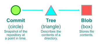
For a quick refresher on how we represent Git objects, see the key below.

Key to how Git objects are represented visually. A green circle represents a commit; a blue triangle represents a tree; and a red box represents a blob.

As discussed in part II, Git’s commit history can be stored in the commit-graph file for fast commit history queries. In this way, Git could walk all of the commits from the haves, then walk to their root trees, then recursively walk trees until finding all trees and blobs reachable from those commits. During this walk, Git can mark each object in-memory with a special flag indicating it is in this reachable set.

To find the reachable set difference, Git can walk from the want objects following each commit parent, root tree, and recursively through the trees. This second walk ignores the objects that were marked in the previous step so each visited object is part of the set difference.

In the figure below, the commit B is a have and the commit A is a want. Two sets are shown. First, everything reachable from B is grouped into a set. The second set is the reachable set difference containing everything reachable from A but not reachable from B.

Figure representing a walk through two commits: a "want" (commit A) and a "have" (commit B).

While this walking algorithm is a natural one to consider, it has a number of significant performance penalties.

First, we will spend a lot of time parsing trees in order to discover their tree entries. We noted in part III that tree parsing is expensive and that was when talking about file history where we only needed to parse trees along a single path. In addition, there are usually many tree entries that point to the same object. For example, an open source license file is usually added once and never modified in a repository. By contrast, almost every commit has a distinct root tree. Thus, each commit introduces a tree with a tree entry pointing to that license file. Git needs to test if the license file is already in the set each time it parses that tree entry. That’s a lot of work. We will revisit how to reduce the time spent parsing trees and following tree entries later, though it will require a new data structure.

The second performance penalty is that this walk requires visiting the entire commit history and likely walking a majority of the Git objects. That cost is paid even if the only objects in the reachable set difference is one commit that changes the README, resulting in a total of one commit, one tree, and one blob in the set difference. The fact that the cost does not scale with the expected output means that even frequent fetches will not reduce this cost.

Thankfully, there is a way to tweak this algorithm to reduce this second cost without needing any new data structures.

Discovering a frontier

If we think about the reachable set difference problem from the perspective of an arbitrary directed graph, then the full walk algorithm of the previous section is the best we can do. However, the Git object graph has additional structure, including different types of objects. Git uses the structure of the commit history to its advantage here, as well as some assumptions about how Git repositories are typically used.

If we think about Git repositories as storing source code, we can expect that code is mostly changed by creating new code. It is rare that we revert changes and reintroduce the exact copy of a code file that existed in the past. With that in mind, walking the full commit history to find every possible object that ever existed is unlikely to be helpful in determining the set of “new” objects.

Instead of walking every object in the full commit history, Git uses the commit history of the haves and wants to discover a frontier of commits. These commits are the commits that are reachable from the haves but are on the boundary between the reachable set difference and the common history. For a commit A to be in the frontier, there must be at least one commit B whose parent is A and B is reachable from the wants but not reachable from the haves.

This idea of a frontier can be visualized using the git log --boundary query with a commit range parameter. In the example below, we are exploring the commits reachable from d02cc45c7a but not reachable from 3d8e3dc4fc. The commits marked with o are on this boundary.

$ git log --graph --oneline --boundary 3d8e3dc4fc..d02cc45c7a
*   acdb1e1053 Merge branch 'mt/checkout-count-fix'
|\
| * 611c7785e8 checkout: fix two bugs on the final count of updated entries
| * 11d14dee43 checkout: show bug about failed entries being included in final report
| * ed602c3f44 checkout: document bug where delayed checkout counts entries twice
* |   f0f9a033ed Merge branch 'cl/rerere-train-with-no-sign'
|\ \
| * | cc391fc886 contrib/rerere-train: avoid useless gpg sign in training
| o | bbea4dcf42 Git 2.37.1
|  /
o / 3d8e3dc4fc Merge branch 'ds/rebase-update-ref'
 /
o e4a4b31577 Git 2.37

Once Git has determined the commit frontier, it can simplify the object walk somewhat. Starting at the frontier, Git walks those root trees and then recursively all of the reachable trees. These objects are marked as reachable from the wants. Then, the second walk from the haves continues as normal, stopping when it sees objects in this smaller set.

Image representing a simplified object walk starting from the the commit frontier. Git walks those root trees and then recursively all of the reachable trees.

With this new algorithm, we see that the cost of the object walk can be much smaller: we expect the algorithm to walk about as many objects as there exist from a few root trees, plus the new objects in the reachable set difference. This could still be a large set, but at least it does not visit every object in the full history. As part of this, we have many fewer repeated tree entries since they are rarely repeated within a walk from a few root trees.

There is an additional cost to this algorithm, though. We might increase the size of the resulting set! If some of the commits in the set difference really are reverts, then they could be “reintroducing” an older object into the resulting set. If this commit reverted the file at a given path, then every commit in the frontier must not have that version of the file at its root tree. This exact revert case is rare enough that these new objects do not account for a significant drawback, but it is worth mentioning.

We can still do better! In the case of a monorepo, that cost of walking all of the trees in the frontier can still be significant. Is there a way that we can compute a reachable set difference more quickly? Yes, but it requires new data structures!

Reachability bitmaps

When considering set arithmetic, such as set differences, a natural data structure to use is a bitmap. Bitmaps represent sets by associating every possible object with a position, and then using an array of bits over those positions to indicate if each object is in the set. Bitmaps are frequently used by application databases as a query index. A bitmap can store a precomputed set of rows in a table that satisfy some property, helping to speed up queries that request data in that set.

The figure below shows how the object graph from the previous figures is laid out so that every object is associated with a bit position. The bitmap at the top has a 1 in the positions corresponding to objects reachable from the commit A. The other positions have value 0 showing that A cannot reach that object.

Figure showing how the object graph from the previous figures is laid out so that every object is associated with a bit position.

Computing the set difference between two bitmaps requires iterating over the bit positions and reporting the positions that have a 1 in the first bitmap and a 0 in the second bitmap. This is identical to the logical operation of “A AND NOT B,” but applied to every bit position.

In this way, Git can represent the reachable sets using bitmaps and then perform the set difference. However, computing each bitmap is at least as expensive as walking all of the reachable objects. Further, as currently defined, bitmaps take at least one bit of memory per object in the repository, which can also become too expensive.

The critical thing that Git does to solve this cost of constructing the bitmaps is by precomputing the reachability bitmaps and storing them on disk. Recall from part I that Git uses compressed object storage files called packfiles to store the object contents. The git repack command takes all of the objects and creates a new packfile along with a pack-index.

The git repack --write-bitmap-index option computes reachability bitmaps at the same time as it repacks the Git object data into a new packfile. Each bit position is associated with an object in the packfile based on the order the objects appear in that packfile. In addition to the .pack and .idx files, a new .bitmap file stores these bitmaps. Git can also store reachability bitmaps across multiple packfiles using a multi-pack-index.

Each reachability bitmap is associated with a single Git commit. The bitmap stores the set of objects reachable from that commit. A .bitmap file can store reachability bitmaps corresponding to one or more commits.

If every commit had a reachability bitmap, then we could compute the reachable set difference from a set of haves and wants using the following process:

  1. Take the bitmap for each ‘have’ commit and merge them together into the union bitmap storing every object reachable from at least one ‘have’ commit.
  2. Take the bitmap for each ‘want’ commit and merge them together into the union bitmap storing every object reachable from at least one ‘want’ commit.
  3. Perform a set difference on the bitmaps created in the previous step.

The figure below shows this third step of performing the set difference on the two reachability bitmaps. The “A – B” bitmap is formed by including a 1 if and only if that position has a 1 in the A bitmap and a 0 in the B bitmap.

Figure showing third step of performing the set difference on the two reachability bitmaps.

Unfortunately, computing and storing a reachability bitmap for every commit in the entire repository is not realistic. First, consider that each bitmap can take up one bit per object in the repository, then multiply that by the number of commits in the repository to get quadratic growth! This isn’t exactly a lower bound on the size of these bitmaps since Git uses a compressed bitmap encoding as well as a form of delta compression between bitmaps. However, the cost of computing and storing each bitmap is still significant.

Even if we were able to store a reachability bitmap for every commit, it is possible that a new commit is pushed to the repository and then is requested by a fetch before a reachability bitmap could be computed for it. Thus, Git needs some way to compute the reachable set difference even when the requested haves and wants do not have pre-computed bitmaps.

Git solves this by using a commit history walk. Starting at the haves, Git walks the commit history until finding a commit that has a precomputed reachability bitmap. That bitmap is used as a starting point, and the commit walk halts when it finds another reachability bitmap or finds a commit that is already contained in the reachable set because its bit is 1 in the bitmap. After the commit set is explored, Git walks the trees starting at the root trees, ignoring any trees that already exist in the reachability bitmap.

In this way, Git can dynamically compute the reachability bitmap containing the full set of objects reachable from the haves. The process is repeated with the wants. Then, the set difference is computed from those two bitmaps.

If the set of precomputed bitmaps is chosen carefully enough and the object order is selected in such a way that the bitmaps compress efficiently, these operations can be done while walking an incredibly small number of objects and using significantly less memory.

With proper maintenance of the reachability bitmap index, these reachable set difference queries can be much faster than the previous frontier walking strategy while also computing the exact set difference. The extra objects that could appear using the frontier algorithm do not appear using the precomputed bitmaps.

If you want to read more about how commits are chosen for bitmaps or how the bitmaps are compressed, read the original announcement of reachability bitmaps which goes into even greater detail. In particular, that post goes very deep on the fact that the object data is sent over the wire using the same packfile format as the on-disk representation discussed in part I, except that Git allows reference deltas to refer to objects already on the client’s machine. The fact that the on-disk representation and the network transfer format use this common format is one of Git’s strengths.

Pushing to a remote

The previous algorithms were focused on computing the reachable set difference required during a git fetch command. After the client sends the list of haves and wants, the server computes the set difference and uses that to send the objects to the client. The natural opposite of this operation is the git push command where the client sends new objects to the server.

We could use the existing algorithm, but we need to flip around some meanings. The haves and wants become commits that “the server has” and “the client wants the server to have”. One caveat is that, by default, git push doesn’t do a negotiation at the start and instead thinks about the references in refs/remotes/<remote> as the set of haves. You can enable the push.negotiate config option if you find this negotiation to be valuable. This negotiation is important if you have not updated your refs/remotes/<remote> references through a git fetch in a while. The negotiation is more useful if you are using background maintenance because you are more likely to have most of the objects the remote will advertise in the negotiation.

Other than reversing the roles of the haves and wants, the goals of git push are exactly the same as git fetch. The command synchronizes objects from one repository to another. However, we can again think about the typical use of the commands to see that there are some asymmetries.

When a client runs git fetch, that command will typically download new objects from several other contributors to that repository, perhaps merged together by pull requests. These changes are likely to include changes to many files across several directories. When a client runs git push, the information that is new to the remote is typically a single topic branch created by a single contributor. The files modified by this effort are likely to be smaller in number than the git fetch case.

Git exploits this asymmetry using a custom reachable set difference algorithm tailored to these expectations.

Sparse reachable set difference

One major asymmetry with git push is that clients rarely find it worth the cost to precompute reachability bitmaps. That maintenance cost is too CPU intensive compared to the number of times git push is run by a typical user. For Git servers, reachability bitmaps are absolutely critical to efficient function, so that extra maintenance is easy to justify.

Without reachability bitmaps, Git falls back to the frontier algorithm when computing the reachable set difference. This works mostly fine for small projects, but when the client repository is very large, the cost of walking every object reachable from even a single root tree becomes too expensive.

This motivated the sparse reachable set difference algorithm. This algorithm is enabled by the pack.useSparse config option, which is now enabled by default. In addition to using the commit history to construct a frontier of commits, the sparse algorithm uses the structure of the trees themselves to compute the reachable set difference.

Just like the frontier algorithm, Git computes the commit frontier as a base of which objects are in common between the haves and wants. Then, instead of walking all the trees reachable from the root trees in the frontier and then walking the root trees from the wants, Git walks these trees in a single walk.

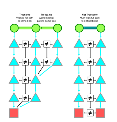
Instead of exploring the object graph directly by walking from tree to tree one at a time, Git changes the walk to do a breadth-first search on the paths available in these trees. Each node of this walk consists of a path and a set of trees. Each tree is marked as uninteresting or interesting, depending on whether they come from the commit frontier or not, respectively.

The walk is initialized with the empty path and the set of root trees from our commit frontier and the commits reachable from the wants. As Git explores a node, it iterates over each tree in the associated set. For each of those trees, it parses the tree entries and considers the path component from each. If the entry points to a blob, then those blobs are marked as interesting or uninteresting. If the entry points to a tree, then the path component leads to a new node and that tree is added to that node’s tree set.

During this walk, uninteresting trees mark their child trees as uninteresting. When visiting a node, Git skips the node if every contained tree is uninteresting.

These “all uninteresting” nodes represent directories where there are no new objects in the reference being pushed relative to the commit frontier. For a large repository and most changes, the vast majority of trees fit in this category. In this way, this sparse algorithm walks only the trees that are necessary to discover these new objects.

Figure representing a sparse algorithm that walks only the trees that are necessary to discover these new objects.

This sparse algorithm is discussed in more detail in the blog post announcing the option when it was available in Git 2.21.0, though the pack.useSparse option was enabled by default starting in Git 2.27.0.

Heuristics and query planning

In this blog series, we are exploring Git’s internals as if they were a database. This goes both directions: we can apply database concepts such as query indexes to frame these advanced Git features, but we can also think about database features that do not have counterparts in Git.

This area of synchronization is absolutely one area where database concepts could apply, but currently do not. The concept I’m talking about is query planning.

When an application database is satisfying a query, it looks at the query and the available query indexes, then constructs a plan for executing the query. Most query languages are declarative in that they define what output they want, but not how to do that operation. This gives the database engine flexibility in how to best use the given information to satisfy the query.

When Git is satisfying a reachable set difference query, it does the most basic level of query planning. It considers its available query indexes and makes a choice on which to use:

  1. If reachability bitmaps exist, then use the bitmap algorithm.
  2. Otherwise, if pack.useSparse is enabled, then use the sparse algorithm.
  3. If neither previous case holds, then use the frontier algorithm.

This is a simple, and possibly unsatisfying way to do query planning. It takes the available indexes into account, but does not check how well those indexes match with the input data.

What if the reachability bitmaps are stale? We might spend more time in the dynamic bitmap computation than we would in the frontier algorithm.

We can walk commits really quickly with the commit-graph. What if there are only a few commits reachable from the wants but not reachable from the frontier? The sparse algorithm might be more efficient than using reachability bitmaps.

This is an area where we could perform some experiments and create a new, dynamic query planning strategy that chooses the best algorithm based on some heuristics and the shape of the commit history.

Already there is some ability to customize this yourself. You can choose to precompute reachability bitmaps or not. You can modify pack.useSparse to opt out of the sparse algorithm.

A change was merged into the Git project that creates a push.useBitmaps config option so you can compute reachability bitmaps locally but also opt out of using them during git push. Reachability bitmaps are integrated with other parts of Git, so it can be helpful to have them around. However, due to the asymmetry of git fetch and git push, the sparse algorithm can still be faster than the bitmap algorithm. Thus, this config will allow you to have the benefits of precomputed reachability bitmaps while also having fast git push commands. Look forward to this config value being available soon in Git 2.38.0!

Come back tomorrow for the final installment!

Now that we’ve explored all of the different ways Git operates on a repository, we have a better grasp on how Git scales its algorithms with the size of the repository. When application databases grow too quickly, many groups resort to sharding their database. In the next (and final!) part of this blog series, we will consider the different ways to scale a Git repository, including by sharding it into smaller components.

I’ll also be speaking at Git Merge 2022 covering all five parts of this blog series, so I look forward to seeing you there!

Отново ще участвам в изборите

Post Syndicated from Bozho original https://blog.bozho.net/blog/3935

Листите за предстоящите избори са внесени и за мен е чест да бъда в два района:

Водач в Ловеч, където ще помогна коалицията да реализира мандат. Там съм по мое предложение – баба ми и нейният род са от Троян и околните махали. Имам ярки спомени от детството по баирите около Троян, а в мазето още има от сливовата ракия на прадядо ми. Там имаме силен местен кандидат на второ място – Свилен Андреев, с когото на практика сме съ-водачи на листата и който се надявам да влезе в парламента за втори път.

Също така съм в 23-ти район (София), плътно след две силни жени – Надежда Йорданова и Кристина Петкова. Изборът в 23-ти район ще е труден, но се радвам, че даваме на избирателите толкова добри опции, между които да се чудят. Преференциите винаги са били инструмент на демократичната общност.

Листите ни са обновени спрямо предните избори и смятам, че са добра отправна точка за силна кампания, в която да убедим повече хора, че системният ни опит да изградим силни институции, които да решават проблемите на хората, е най-важната задача.
Институции, които могат ефективно, а не ефектно да се борят с корупцията; институции, които повишават здравето, а не сметката за лекарства; които дават образование, а не просто диплома; които си вършат бюрократичната работа, а не я пренасят върху гражданите и бизнеса.

Кампанията започва на втори септември. Ще бъда на улицата, сред хората, в София, Ловеч, Троян, Луковит, Тетевен и другите населени места в района.

Материалът Отново ще участвам в изборите е публикуван за пръв път на БЛОГодаря.

Clever Phishing Scam Uses Legitimate PayPal Messages

Post Syndicated from Bruce Schneier original https://www.schneier.com/blog/archives/2022/09/clever-phishing-scam-uses-legitimate-paypal-messages.html

Brian Krebs is reporting on a clever PayPal phishing scam that uses legitimate PayPal messaging.

Basically, the scammers use the PayPal invoicing system to send the email. The email lists a phone number to dispute the charge, which is not PayPal and quickly turns into a request to download and install a remote-access tool.

[$] Python multi-level break and continue

Post Syndicated from original https://lwn.net/Articles/906512/

A fairly lengthy discussion of whether there should be a way to
break out of (or
continue) more than one level of nested loops in Python recently
took place in the Ideas
category
of the language’s discussion forum. The idea is
attractive, at least in an abstract sense—some other languages support
jumping out of
multiple loops at once—but it seems unlikely to go anywhere for Python.
The barrier to new features is fairly high, for sure, but there is also a
need for proponents to provide real-world examples that demonstrate their
advantages. That, too, is a difficult bar to clear, as was seen in the
discussion.

Amazon DevOps Guru increases Operational Efficiency for 605

Post Syndicated from Mohit Gadkari original https://aws.amazon.com/blogs/devops/amazon-devops-guru-increases-operational-efficiency-for-605/

605 is an independent TV measurement firm that offers advertising and content measurement, full-funnel attribution, media planning, optimization, and analytical solutions, all on top of their multi-source viewership data set covering over 21 million U.S. households. 605 has built their technology solutions on AWS with dozens of accounts and tens of thousands of resources to monitor.

As 605 continues to innovate and build new solutions, the size and complexity of their AWS deployment has also grown proportionally. Over time, managing their deployment has become an operational challenge for their current team. 605 has deployed different application performance monitoring (APM) tools and notification systems to help their observability staff scale and support their growing cloud environment. However, 605 realized that their continued growth on the cloud would necessitate either increasing their observability staff or assuming some risk of potential application performance issues or even outages.

Amazon DevOps Guru allowed 605 to find a third path forward. Rather than accepting the trade-off of hiring more staff or assuming more risk, 605 discovered that DevOps Guru provides an increase in operational efficiency using their existing staff resources by applying artificial intelligence (AI) to supplement their existing APM and notification platform. Layering DevOps Guru into their DevOps environment , 605 realized a 4-fold decrease in the number of alerts and notifications that proved to be false positives. In fact, 605 went from an environment where 76.2% of their alerts and notifications were false positives, to one with only 18.9% false positives simply by adding Amazon DevOps Guru. In the end, 605 can more effectively and efficiently manage their environment with existing resources and actually freeing-up DevOps brainpower to work on more strategically important initiatives than application management.

“Amazon DevOps Guru has provided insights that help us focus our infrastructure roadmap. Our current SIEM tools require building out alerting ahead of time, while DevOps Guru is constantly evolving, which prevents becoming stagnant in our monitoring. Reducing the risk of false positive alerts has saved countless engineering hours.”

Jared Williams, VP of Infrastructure and Architecture, 605

605 without DevOps Guru had their Amazon CloudWatch and Amazon Elastic Container Service for Kubernetes ( Amazon EKS) configured with different application performance monitoring and notification systems. They saw only 23.8 % legitimate alerts and notifications, where as with the integration with DevOps Guru the legitimate alerts and notifications went up to 81% for a 6-month time period.
605 are monitoring over 13+ AWS Accounts, 20+ Amazon EKS Clusters, 500+ Pods ,15000+ EC2 Instances, 500+ S3 Buckets and 55+ Application Load Balancers with DevOps Guru

605 without DevOps Guru had their Amazon CloudWatch and Amazon Elastic Container Service for Kubernetes ( Amazon EKS) configured with different application performance monitoring and notification systems. They saw only 23.8 % legitimate alerts and notifications, where as with the integration with DevOps Guru the legitimate alerts and notifications went up to 81% for a 6-month time period.

Figure 1. 605 are monitoring over 13+ AWS Accounts, 20+ Amazon EKS Clusters, 500+ Pods ,15000+ EC2 Instances, 500+ S3 Buckets and 55+ Application Load Balancers with DevOps Guru.

Amazon DevOps Guru is a service powered by applying artificial intelligence (AI) that’s designed to make it easy to improve an application’s operational performance and availability. DevOps Guru helps detect behaviors that deviate from normal operating patterns so that you can identify operational issues long before they impact your applications. DevOps Guru utilizes ML models informed by years of Amazon.com and AWS operational excellence to identify anomalous application behavior (for example, increased latency, error rates, resource constraints, and others). Furthermore, it helps surface critical issues that could cause potential outages or service disruptions. When DevOps Guru identifies a critical issue, it automatically sends an alert and provides a summary of related anomalies, the likely root cause, and context for when and where the issue occurred. When possible, DevOps Guru also helps provide recommendations regarding how to remediate the issue. DevOps Guru ingests operational data from your AWS applications and provides a single dashboard to visualize issues in your operational data. DevOps Guru can be enabled for all of the resources in your AWS account, resources in your AWS CloudFormation Stacks, or resources grouped together by AWS Tags, with no manual setup or ML expertise required.

The value of DevOps Guru for 605 goes beyond providing operational efficiency and avoiding the choice of adding DevOps resources or assuming more risk. DevOps Guru also discovered issues with application performance that their existing solutions weren’t trained to inspect.

This new data allowed 605 to avoid a potential problem that they didn’t otherwise know would occur. As DevOps Guru doesn’t require any set-up beyond enabling the service and choosing resources to monitor (it’s a managed service), the service can surface issues without any prior configuration.

In the end, the value of DevOps Guru for 605 surfaces in three ways. First, it increases operational efficiency by allowing their existing DevOps team to more effectively manage its AWS applications and resources, as well as the room to grow along with their business needs. Second, DevOps Guru reduces operational fatigue and allows their DevOps teams to focus on more strategic issues by significantly reducing false positives. Lastly, DevOps Guru can find operational issues to which existing APM tools may not be configured or able to detect.

Start monitoring your AWS applications with AWS DevOps Guru today using this link

About the authors:

Mohit Gadkari

Mohit Gadkari is a Solutions Architect at Amazon Web Services (AWS) supporting SMB customers. He has been professionally using AWS since 2015 specializing in DevOps and Cloud Security and currently he is using this experience to help customers navigate the cloud.

Pauly Longani

Pauly is an Enterprise Support Lead at AWS, USA. He is a customer advocate and supports his customers in their cloud journey. He is passionate about the cloud and how it can be leveraged to overcome challenges across industry verticals.

Jared Williams

Jared, VP of Infrastructure and Architecture at 605, is in his 15th year managing or working on teams with DevOps type focuses. He has been involved with AWS since 2009. He manages the multi-team DevOps department at 605 where he has been for more than three years. Jared also co-founded a 24,000+ person DevOps community.

[Security Nation] Gordon “Fyodor” Lyon on Nmap, the Open-Source Security Scanner

Post Syndicated from Rapid7 original https://blog.rapid7.com/2022/08/31/security-nation-gordon-fyodor-lyon-on-nmap-the-open-source-security-scanner/

[Security Nation] Gordon “Fyodor” Lyon on Nmap, the Open-Source Security Scanner

In this episode of Security Nation, Jen and Tod chat with Gordon “Fyodor” Lyon, author of the widely used open-source Nmap Security Scanner. On the doorstep of Nmap’s 25th anniversary, Gordon and our hosts talk about the tool’s impact on asset management, as well as the struggles and triumphs of creating and managing the solution. They even cover a few highlights from Hollywood films where Nmap makes a guest appearance.

Stick around for our Rapid Rundown, where Tod and Jen talk about a recent warning from the FBI that decentralized finance (DeFi) – i.e., cryptocurrency – poses some unique risks, which attackers are already exploiting.

Gordon “Fyodor” Lyon

[Security Nation] Gordon “Fyodor” Lyon on Nmap, the Open-Source Security Scanner

Gordon “Fyodor” Lyon authored the open-source Nmap Security Scanner in 1997 and continues to coordinate its development. His company also develops and sells Npcap, a raw networking library and driver for Windows. Npcap is now used in hundreds of other software projects, including Wireshark and Microsoft Defender for Identity. Gordon is a founding member of the Honeynet Project and served on the technical advisory boards for Qualys and AlienVault, as well as editorial boards for many conferences and journals. He authored or co-authored the books “Nmap Network Scanning,” “Know Your Enemy: Honeynets,” and “Stealing the Network: How to Own a Continent.” He runs the “Full Disclosure” mailing list, along with popular security resource sites such as SecLists.Org, SecTools.Org, and Insecure.Org.

Show notes

Interview links

  • Check out Nmap if, for some reason, you haven’t already.
  • Learn about Npcap, the packet capture library tool that Gordon and his company also offer.
  • Watch Gordon and HD Moore, the creator of Metasploit, chat about the evolution of network scanning on YouTube.

Rapid Rundown links

Like the show? Want to keep Jen and Tod in the podcasting business? Feel free to rate and review with your favorite podcast purveyor, like Apple Podcasts.

Want More Inspiring Stories From the Security Community?

Subscribe to Security Nation Today

Media Workflowing to Europe: IBC 2022 in Amsterdam Preview

Post Syndicated from Jeremy Milk original https://www.backblaze.com/blog/media-workflowing-to-europe-ibc-2022-in-amsterdam-preview/

You can send media in milliseconds to just about every corner of the earth with an origin store at your favorite cloud storage company and a snappy content delivery network (CDN). Sadly, delivering people to Europe is a touch more complicated and time intensive. Nevertheless, the Backblaze team is saddling up planes, trains, and automobiles to bring the latest on media workflows to the attendees of IBC 2022. Whether you’re there in person or virtually, we’ll be discussing and demo-ing all the newest Backblaze B2 Cloud Storage solutions that will ensure your data can travel with ease—no mass transit needed—everywhere you need it to be.

Learn More LIVE in Amsterdam

If you’re attending the IBC 2022 conference in Amsterdam, join us at stand 7.B06 to learn about integrating B2 Cloud Storage into your workflow. Stop by anytime or you can schedule a meeting here. We’d love to see you.

IBC 2022 Preview: What’s New for Backblaze B2 Media Workflow Solutions

Our stand will have all the usual goodness: partners, friendly faces, spots to take a load off and talk about making your data work harder, and, of course, some next-level SWAG. Let’s get into what you can expect.

New Pricing Models and Migration Tools

Our team is on hand to talk you through two new offerings that have been generating a lot of excitement among teams across media organizations:

  • Backblaze B2 Reserve: You can now purchase the Backblaze service many know and love in capacity-based bundles through resellers. If your team needs 100% budget predictability and would like waived transaction fees and premium support included as well, you should check out this new pricing model. Check it out here.
  • Universal Data Migration: This IBC 2022 Best of Show nominee makes it easy and FREE to move data into Backblaze from legacy cloud, on-premises, and LTO/tape origins. If your current data storage is holding your team or your budget back, we’ll pay to free your media and move it to B2 Cloud Storage. Learn more here.

Six Flavors of Media Workflow Deep Dives

We’ve gathered materials and expertise to discuss or demo our six most asked about workflow improvements. We’re happy to talk about many other tools and improvements, but here are the six areas we expect to talk about the most:

  1. Moving more (or all) media production to the cloud. Ensuring everyone—clients, collaborators, employers, everyone—has easy real-time access to content is essential for the inevitable geographical distribution of modern media workflows.
  2. Reducing costs. Cloud workflows don’t need to come with costly gotchas, minimum retention penalties, and/or high costs when you actually want to use your content. We’ll explain how the right partners will unlock your budget so you can save on cloud services and spend more on creative projects.
  3. Streamlining delivery. Pairing cloud storage with the right CDN is essential to make sure your media is consumable and monetizable at the edge. From streaming services to ecommerce outlets to legacy media outlets, we’ve helped every type of media organization do more with their content.
  4. Freeing storage. Empty your expensive on-prem storage and stop adding HDs and tapes to the pile by moving finished projects to always-hot cloud storage. This doesn’t just free up space and money: Instantly accessible archives means you can work with and monetize older content with little friction in your creative process.
  5. Safeguarding content. All those tapes or HDs on a shelf, in the closet, or wherever you keep them are hard to manage and harder to access and use. Parking everything safely and securely in the cloud means all that data is centrally accessible, protected, and available for more use.
  6. Backing up (better!). Yes, we’ve got roots in backup going back >15 years—so when it comes to making sure your precious media is protected with easy access for speedy recovery, we’ve got a few thoughts (and solutions).

Partners, Partners, and More Partners…

“The more we get together, the happier we’ll be,” might as well be the theme lyric of cloud workflows. Combining best of breed platforms unlocks better value and functionality, and offers you the ability to build your cloud stack exactly how you need it for your business. We’ve got a massive ecosystem of integration partners to bring to bear on your challenges, and we’re happy to share our IBC 2022 stand with two incredible members of that group: media management and collaboration company iconik and the cloud NAS platform LucidLink.

We’ll be demoing a brand new, free Backblaze B2 Storage Plug-in for iconik which enables users of Backblaze, iconik, and LucidLink to move files between services in just a click–we’d love to walk you through it.

Hoping We Can Help You Soon

Whether it’s in person at IBC 2022 or virtually when it works for you, we’d love to walk you through any of the solutions we can serve for hardworking media teams. If you will be in Amsterdam, schedule a meeting to ensure you’ll get the right expert on our team, then stick around for the swag and good times. If you’re not making the trip, please reach out to to us here where we can share all of the same information.

The post Media Workflowing to Europe: IBC 2022 in Amsterdam Preview appeared first on Backblaze Blog | Cloud Storage & Cloud Backup.

Learn more about the new allow list feature in Macie

Post Syndicated from Jonathan Nguyen original https://aws.amazon.com/blogs/security/learn-more-about-the-new-allow-list-feature-in-macie/

Amazon Macie is a fully managed data security and data privacy service that uses machine learning and pattern matching to discover and help you protect your sensitive data in Amazon Web Services (AWS). The data that is available within your AWS account can grow rapidly, which increases your need to verify that all sensitive data is identified and protected. Macie provides you with the ability to use both managed data identifiers and custom data identifiers, but enabling these identifiers for every job could result in a large number of security findings that might not take into account how data is used within your AWS account. So that you can tailor the detection and creation of findings within Macie, Macie now has an allow list feature available for use with your scanning jobs.

In this blog post, we show you how to set up an allow list in Macie and run a Macie scan that uses the allow list to ignore the specified values when creating sensitive data findings. The allow list feature can help your sensitive data management team by reducing false positives due to data text or formats in your environment that do not require action. This makes it easier for your team to focus on Macie findings that need to be reviewed and remediated. By increasing the overall confidence in findings presented by Macie, you can improve the performance of automated workflows and solutions.

Prerequisites

To get started, you’ll need the following prerequisites:

  1. An active AWS account
  2. Amazon Macie enabled within your AWS account
  3. (Optional) Member AWS accounts are enabled using AWS Organizations and a delegated Macie administrator account

Create an allow list in Macie

You can configure allow lists with either regular expressions (regex) or predefined text. Use a predefined text allow list if you have a list of specific values you want to exclude, like a list of example fake names or addresses that are used in test data sets. Alternatively, if you don’t have the exact values but know the pattern to exclude, you can use a regex allow list. Some use cases for a regex allow list could be to exclude tracking IDs or public reference numbers that could resemble a Macie managed data identifier or custom data identifier.

It is important to note that allow lists, and S3 objects if using predefined text, must be created in the same AWS account where the Macie job is created.

  1. If Macie jobs are created from the Macie delegated administrator AWS account to scan member AWS accounts, then the allow lists must be centrally configured in the Macie delegated administrator account.
  2. If Macie jobs are created from the member AWS account to scan buckets within the same AWS account, then the allow lists must be configured in the same AWS account where the Macie job is created.

To create an allow list by using the Amazon Macie Console

  1. In the Amazon Macie Console, navigate to Macie.
  2. Under Settings, choose Allow lists.
  3. Choose Create.
  4. Choose a list type.
    1. If you’re creating a regex allow list, choose Regular expression. For List settings, enter the following settings for the allow list.
      1. For Name, enter the name of the list.
      2. For Description, enter a description (optional).
      3. For Regular expression, enter the regular expression. Macie will not create findings for any matches on the allow list regex.
      4. Evaluate with sample data if needed to test your regex. Macie provides an Evaluate option so you can test your regex against sample data sets to make sure it’s working as expected.
    2. If you’re creating a predefined text allow list, choose Predefined text. For this option, you will need to create a plaintext file and upload the file to an Amazon Simple Storage Service (Amazon S3) bucket. Once you upload the file, you can then reference the Amazon S3 object in the allow list.
      1. Enter the name of the list.
      2. Enter a description for the list (optional).
      3. Enter the S3 bucket name.
      4. Enter the S3 object name of the plaintext file.

    Note: The Macie service-linked role must have the ability to read the S3 object for the predefined text. When you run Macie jobs that use allow lists with predefined text, the Macie service-linked role will read the S3 object. If there is any error reading the S3 object, the Macie job will continue to run without using the predefined text allow list. You will need to periodically check your allow lists to make sure they are in an OK status. You can check the status of each allow list in the Amazon Macie console or via the AWS CLI using the get-allow-list API.

    More information and explanation for status of allow list can be found in the Amazon Macie User Guide.

  5. Choose Create to create the allow list.

    Note: An allow list must be stored in an S3 bucket in the same AWS account and AWS Region as your Macie account. Macie cannot access an allow list if it is stored in a different Region or account.

You can also create and manage allow lists by using the Amazon Macie console, AWS Command Line Interface (AWS CLI) or AWS CloudFormation.

To create or manage an allow list by using the AWS CloudFormation

Below is an example enabling Amazon Macie for an account. The session resource configures Macie to publish updated policy findings for the account.

AWSTemplateFormatVersion: 2010-09-09
Description:<insert-template-description>
Resources:
  EnableMacieSession:
Type: AWS::Macie::Session
Properties:
    	    FindingPublishingFrequency: <insert-finding-publishing-frequency>
    Status: ENABLED

Below is an example of creating an allow list that uses a regular expression to specify a text pattern to ignore. Like other Macie resources, the DependsOn attribute is a required dependency for creating a Macie allow list.

AWSTemplateFormatVersion: 2010-09-09
Description:<insert-template-description>
Resources:
  RegularExpressionAllowList:
Type: AWS::Macie::AllowList
DependsOn: Session
Properties:
  Criteria:
    Regex: “<insert-regex-expression>”
  Description: <insert-allow-list-description>
  Name: <insert-allow-list-name>
  Tags:
    - Key: <insert-tag-key-name>
      Value: <insert-tag-key-value>

Below is an example creating an allow list that specifies a list of predefined text to ignore.

AWSTemplateFormatVersion: 2010-09-09
Description:<insert-template-description>
Resources:
PredefinedAllowList:
Type: AWS::Macie::AllowList
DependsOn: Session
Properties:
  Criteria:
    S3WordsList:
      BucketName: <DOC-EXAMPLE-BUCKET>
      ObjectKey: <OBJECT-EXAMPLE-KEY>
  Description: <insert-allow-list-description>
  Name: <insert-allow-list-name>
  Tags:
  - Key: <insert-tag-key-name>
    Value: <insert-tag-key-value>

To create or manage an allow list by using the AWS CLI

  1. In the AWS CLI, run the following commands to create an allow list with a regular expression.
    aws macie2 create-allow-list \
    --criteria '{"regex":"<insert-regex-expression>"}' \
    --name "<insert-allow-list-name>" \
    --description "<insert-allow-list-description>"
  2. In the AWS CLI, run the following commands to create an allow list with predefined text.
    aws macie2 create-allow-list \
    --criteria '{"s3WordsList":{"bucketName":"<DOC-EXAMPLE-BUCKET>","objectKey":"<OBJECT-EXAMPLE-KEY>"}}' \
    --name "<insert-allow-list-name>" \
    --description "<insert-allow-list-description>"
  3. In the AWS CLI, run the following commands to update an existing allow list.
    aws macie2 update-allow-list --id <GUID-for-Macie-allow-list> example --description <insert-new-description>
  4. In the AWS CLI, run the following commands to delete an existing allow list.
    aws macie2 delete-allow-list --id <GUID-for-Macie-allow-list> example --ignoreJobChecks false
  5. In the AWS CLI, run the following commands to get existing allow lists.
    aws macie2 get-allow-list –id <GUID-for-Macie-allow-list>

For a detailed list of available AWS CLI commands, refer to the AWS CLI documentation for Amazon Macie.

Use the allow list in a Macie scan

After you create allow lists, you can create and run sensitive data discovery jobs in Macie. This will enable you to review, analyze, and compare findings about the affected resources in Amazon S3 buckets with or without allow lists.

Option 1: Create a Macie job with the allow list by using the console

  1. Go to the Amazon Macie Console and navigate to Macie.
  2. In the navigation pane, choose Jobs, and then choose Create job.
  3. On the Choose Amazon S3 buckets page, choose Select specific buckets.

    Note: Macie displays a list of all the buckets managed by your AWS account, including members if configured, in the current Region.

    • Under Select Amazon S3 buckets, optionally choose Refresh to retrieve the latest bucket metadata from Amazon S3.
  4. In the table, select each bucket you want the job to analyze, and then choose Next.
  5. Review and optionally adjust the list of S3 buckets that you selected for the job, and then choose Next.
  6. Refine the scope of the job, if needed. Use these settings to specify how often you want the job to run and the depth and scope of the job’s analysis, and then choose Next.
  7. Select any managed data identifiers you want to use, and then choose Next.
  8. Select any custom data identifiers that you want to use, and then choose Next.
  9. Select the allow lists that you created to ignore either predefined text or regular expression patterns for any objects in the job, and then choose Next.

    Figure 1: Selecting allow lists for a Macie job

    Figure 1: Selecting allow lists for a Macie job

  10. In General settings, enter a name for the job. You can also enter a description and assign tags to the job. Choose Next.
  11. Review and create the job, and then choose Submit.

Option 2: Create a Macie job with the allow list by using the AWS CLI

  1. In the AWS CLI, run the following command.
    aws macie2 create-classification-job \
    --generate-cli-skeleton > <insert-macie-job-input-json>
  2. Input the GUID for the Macie allow list as part of the Macie job input in the JSON file.
  3. Run the following command.
    aws macie2 create-classification-job \
    --cli-input-json file://<insert-macie-job-input-json>

Review Macie findings before and after allow lists

It is important to note that for any existing jobs you configured in your AWS account or organization prior to the Macie allow list feature being released, you will need to recreate those Macie jobs and reference the allow lists you want the job to use. This is only required if you want to have existing jobs use allow lists.

Before you run a Macie job that uses predefined text allow lists, verify that existing Amazon Key Management Service (AWS KMS) keys that are used to encrypt buckets and S3 bucket policy grant the Macie service-linked role the necessary permissions to decrypt the S3 objects.

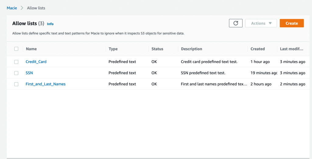
Figure 2 shows an example of predefined text allow lists for sensitive data discovery jobs, that include credit card numbers, Social Security Numbers (SSNs), and first and last names. The values in the S3 object allow lists will not create Macie findings when the sensitive data discovery job inspects S3 objects.

Figure 2: Example list of existing allow lists

Figure 2: Example list of existing allow lists

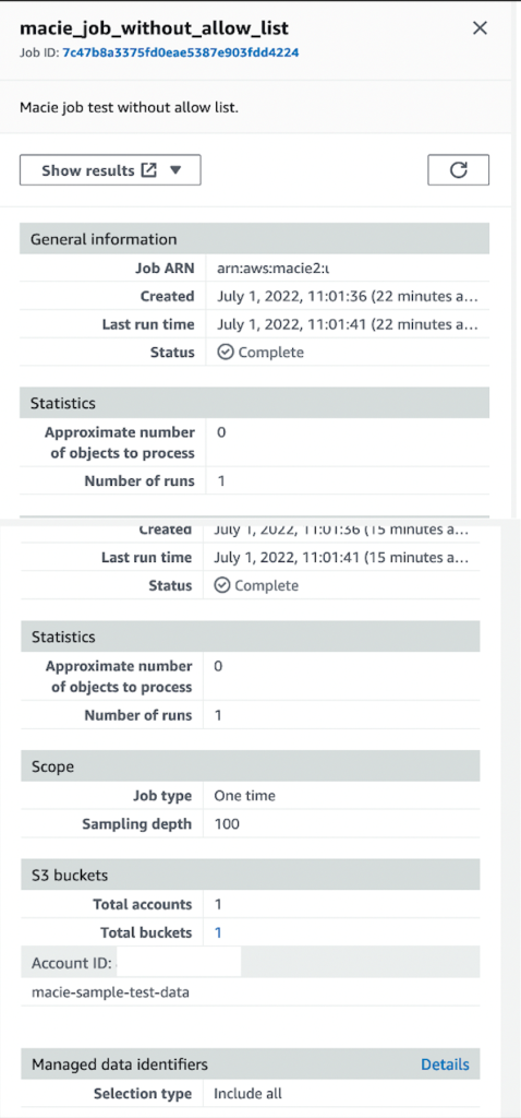
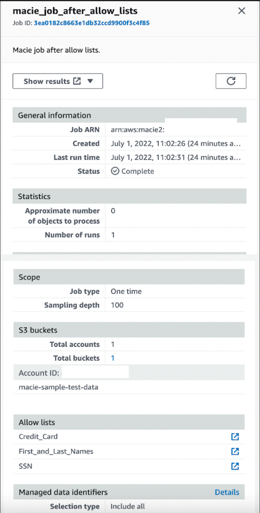
Figure 3 shows a sensitive data discovery job that does not include the predefined text allow lists.

Figure 3: Macie job example without allow list configured

Figure 3: Macie job example without allow list configured

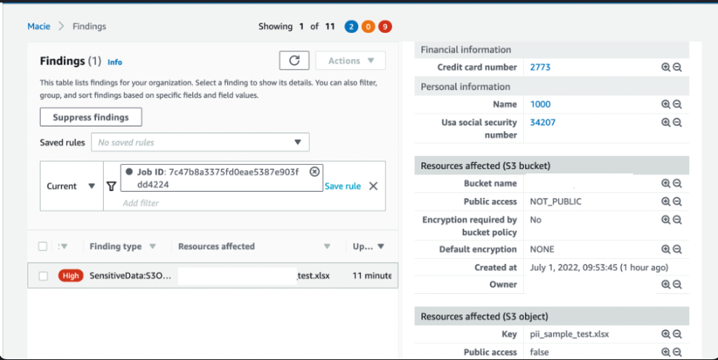
Since there are no allow lists configured, Macie creates findings for credit card numbers, United States SSNs, and names, as shown in Figure 4.

Figure 4: Macie job scan without allow list results

Figure 4: Macie job scan without allow list results

Figure 5 shows a sensitive data discovery job that does include the use of a predefined text allow lists.

Figure 5: Macie job example with allow list configured

Figure 5: Macie job example with allow list configured

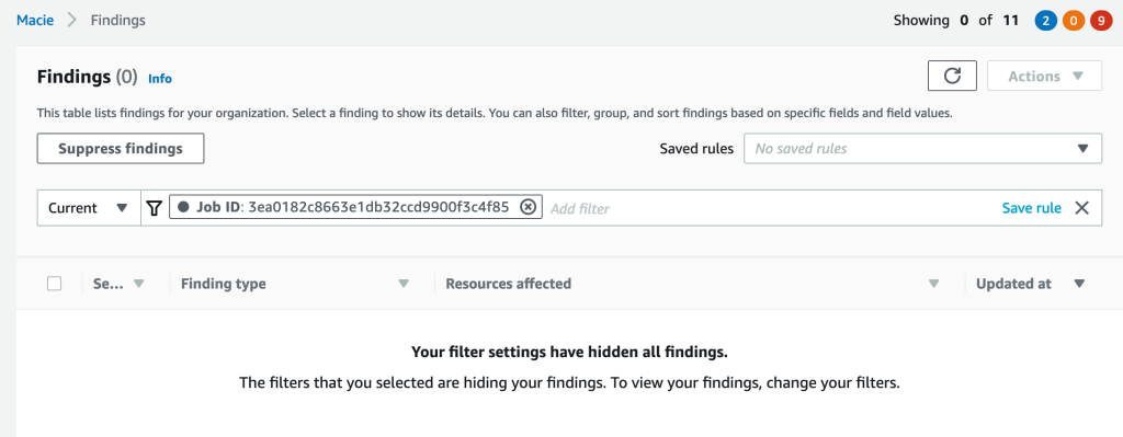
Because we have configured an allow list for this job, Macie creates no findings for credit card numbers, United States SSNs, and names. Figure 6 shows the lack of findings.

Figure 6: Macie job results with allow list configured

Figure 6: Macie job results with allow list configured

Conclusion

In this post, we walked through how to create, manage, and use Macie allow lists with your Macie jobs. Reducing Macie false-positive findings can help your security team to efficiently identify and protect sensitive data within your AWS environment.

Now that we’ve showed you how to create an allow list in Macie, you can use this feature to tailor Macie in your AWS environment, based on your use cases and workloads. After you’ve reduced the false positives in your environment, you can start looking at how to add in automation to respond to Macie findings with allow lists configured.

Try implementing the solution in this blog post for auto-remediation behavior based on finding type and finding severity. Alternatively, since Macie is automatically integrated with AWS Security Hub, you could implement this automated solution to respond to Macie findings by using by Security Hub custom actions.

If you have feedback about this post, submit comments in the Comments section below. If you have questions about this post, contact AWS Support.

Want more AWS Security news? Follow us on Twitter.

Jonathan Nguyen

Jonathan Nguyen

Jonathan is a Shared Delivery Team Senior Security Consultant at AWS. His background is in AWS Security with a focus on threat detection and incident response. Today, he helps enterprise customers develop a comprehensive security strategy and deploy security solutions at scale, and he trains customers on AWS Security best practices.

Ajay Rawat

Ajay Rawat

Ajay is a Security Consultant in a shared delivery team at AWS. He is a technology enthusiast who enjoys working with customers to solve their technical challenges and to improve their security posture in the cloud.

New row and column interactivity options for tables and pivot tables in Amazon QuickSight – Part 2

Post Syndicated from Bhupinder Chadha original https://aws.amazon.com/blogs/big-data/part-2-new-row-and-column-interactivity-options-for-tables-and-pivot-tables-in-amazon-quicksight/

Amazon QuickSight is a fully-managed, cloud-native business intelligence (BI) service that makes it easy to create and deliver insights to everyone in your organization or even with your customers and partners. You can make your data come to life with rich interactive charts and create beautiful dashboards to share with thousands of users, either directly within a QuickSight application or embedded in web apps and portals.

In the previous post in this two-part series, we discussed drag handlers to alter height and width for rows, columns, and table headers. Now, let’s look at some of the new interactivity options for rows and columns for tables and pivot tables.

Hide or show fields for authors

Previously, authors could only hide fields in tables. Now we’re extending this feature to pivot tables as well. Authors can hide rows, columns, and values from either the field wells or from the column or row field headers in pivot tables. For easier identification, hidden fields are indicated with a cross eye icon; you can revert them back to visible using the Show all hidden fields option.

Let’s look at some of the use cases where this could be helpful:

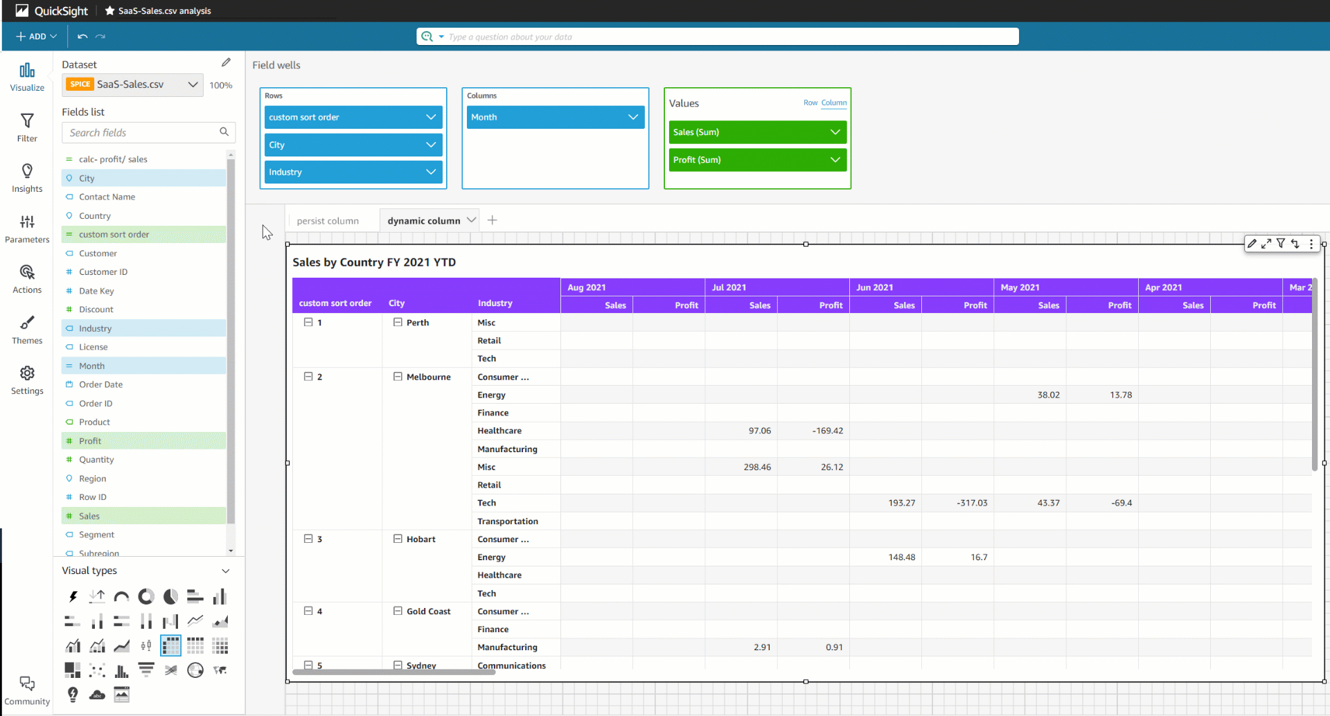
  • Define actions on a pivot table and hide fields to save real estate – Sometimes, you may want to hide fields in a pivot table whose sole purpose is to enable actions, like opening another webpage and pass this hidden field as a parameter.
  • Use hidden fields to define a custom sort order – You can define a custom sort order for your pivot table using hidden fields, for example, defining a specific order for your PNL reports.
  • Display two tables side by side as a single visual – In the following example, we show sales by country, where table 1 displays the last 4 weeks of data and table 2 displays monthly data from the last 4 weeks.
  • Create butterfly tables – Another variation of displaying tables side by side is to create butterfly tables where values are displayed on both sides of the dimension. This is a great way to compare two sets of values. For example, you can compare the current month vs. a full year of data.

Export hidden fields for authors and readers

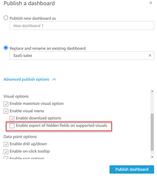
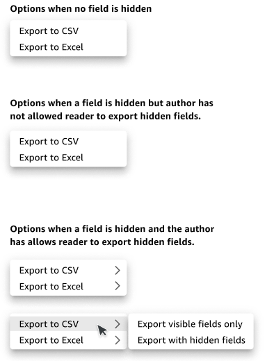
Not only can authors hide fields, they can also control the ability for readers to export data including the hidden fields or without them. When publishing the analysis, authors have the new option Enable export of hidden fields on supported visuals. When you select this option, readers are able to include hidden fields when exporting their data. The default setting is to keep this disabled and only allow readers to export visible data.

Based on the different scenarios, the following options show up for exporting data to CSV and Excel from tables and pivot tables.

Summary

In this post, we looked at the new capability of toggling row, column, and value field visibility on tables and pivot tables. We also discussed the various use cases for hiding fields and the new exporting options associated with field visibility, which can be controlled by authors. To learn more about table and pivot table formatting options, refer to Formatting tables and pivot tables in Amazon QuickSight.

Try out the new feature and share your feedback and questions in the comments section below.


About the author

Bhupinder Chadha is a senior product manager for Amazon QuickSight focused on visualization and front end experiences. He is passionate about BI, data visualization and low-code/no-code experiences. Prior to QuickSight he was the lead product manager for Inforiver, responsible for building a enterprise BI product from ground up. Bhupinder started his career in presales, followed by a small gig in consulting and then PM for xViz, an add on visualization product.

Store Amazon EMR in-transit data encryption certificates using AWS Secrets Manager

Post Syndicated from Hao Wang original https://aws.amazon.com/blogs/big-data/store-amazon-emr-in-transit-data-encryption-certificates-using-aws-secrets-manager/

With Amazon EMR, you can use a security configuration to specify settings for encrypting data in transit. When in-transit encryption is configured, you can enable application-specific encryption features, for example:

  • Hadoop HDFS NameNode or DataNode user interfaces use HTTPS
  • Hadoop MapReduce encrypted shuffle uses Transport Layer Security (TLS)
  • Presto nodes internal communication uses SSL/TLS (Amazon EMR version 5.6.0 and later only)
  • Spark component internal RPC communication, such as the block transfer service and the external shuffle service, is encrypted using the AES-256 cipher in Amazon EMR versions 5.9.0 and later
  • HTTP protocol communication with user interfaces such as Spark History Server and HTTPS-enabled file servers is encrypted using Spark’s SSL configuration

The security configuration of Amazon EMR allows you to set up TLS certificates to encrypt data in transit. A security configuration provides the following options to specify TLS certificates:

  • As a path to a .zip file in an Amazon Simple Storage Service (Amazon S3) bucket that contains all certificates
  • Through a custom certificate provider as a Java class

In many cases, company security policies prohibit storing any type of sensitive information in an S3 bucket, including certificate private keys. For that reason, the only remaining option to secure data in transit on Amazon EMR is to configure the custom certificate provider.

In this post, I guide you through the configuration process and provide Java code samples to secure data in transit on Amazon EMR by storing TLS custom certificates using AWS Secrets Manager.

Secrets Manager helps you protect secrets needed to access your applications, services, and IT resources. The service enables you to easily rotate, manage, and retrieve database credentials, API keys, and other secrets throughout their lifecycle. Users and applications retrieve secrets with a call to Secrets Manager APIs, eliminating the need to hardcode sensitive information in plain text.

Solution overview

The following diagram illustrates the solution architecture.

During an EMR cluster start, if a custom certificate provider is configured for in-transit encryption, the provider is called to get the certificates. A custom certificate provider is a Java class that implements the TLSArtifactsProvider interface.

To make this solution work, you need a secure place to store certificates that can also be accessed by Java code. This post uses Secrets Manager, which provides a mechanism for managing certificates, and encrypts them using AWS Key Management Service (AWS KMS) keys.

To implement this solution, you complete the following high-level steps:

  1. Create a certificate.
  2. Store your certificate to Secrets Manager.
    1. Create a secret for a private key.
    2. Create a secret for a public key.
  3. Implement TLSArtifactsProvider.
  4. Create the Amazon EMR security configuration.
  5. Modify the Amazon Elastic Compute Cloud (Amazon EC2) instance profile role to get the certificate from Secrets Manager.
  6. Start the Amazon EMR cluster.

Create a certificate

For demonstration purposes, this post uses OpenSSL to create a self-signed certificate. See the following code:

openssl req -x509 -newkey rsa:4096 -keyout privateKey.pem -out certificateChain.pem -days 365 -subj "/C=US/ST=MA/L=Boston/O=EMR/OU=EMR/CN=*.ec2.internal" -nodes

This command creates a self-signed, 4096-bit certificate. For production systems, we recommend using a trusted certificate authority (CA) to issue certificates.

The command above has the following parameters:

  • keyout – The output file in which to store the private key.
  • out – The output file in which to store the certificate.
  • days – The number of days for which to certify the certificate.
  • subj – The subject name for a new request. The common name (CN) must match the domain name specified in DHCP that is assigned to the virtual private cloud (VPC). The default is ec2.internal. The * prefix is the wildcard certificate.
  • nodes – Allows you to create a private key without a password, which is without encryption.

The output of OpenSSL includes a pair of keys—one private and one public:

  • privateKey.pem – SSL private key certificate
  • certificateChain.pem – SSL public key certificate

Store your certificate to Secrets Manager

In this section, we walk through the steps to create secrets for a private key and a public key.

Create a secret for a private key

To create a secret for a private key, complete the following steps:

  1. On the Secrets Manager console, choose Store a new secret.
  2. For the secret type, select Other type of secrets.
  3. On the Plaintext tab in the Key/value pairs section, copy the content from privateKey.pem.
  4. For Encryption key, choose DefaultEncryptionKey.
  5. Choose Next.
  6. For Secret name, enter emrprivate.
  7. For Resource permissions, optionally add or edit a resource policy to access secrets across AWS accounts. For more information, refer to Permissions policy examples.
  8. Choose Next.
  9. Choose Store.

Create a secret for a public key

To create a secret for a public key, complete the following steps:

  1. On the Secrets Manager console, choose Store a new secret.
  2. For the secret type, select Other type of secrets.
  3. On the Plaintext tab in the Key/value pairs section, copy the content from certificateChain.pem.
  4. For Encryption key, choose DefaultEncryptionKey.
  5. Choose Next.
  6. For Secret name, enter emrcert.
  7. For Resource permissions, optionally add or edit a resource policy to access secrets across AWS accounts.
  8. Choose Next.
  9. Choose Store.

Implement TLSArtifactsProvider

This section describes the flow in the Java code only. You can download the full code from GitHub.

The interface uses the getTlsArtifacts method, which expects certificates in return:

Java class EmrTlsFromSecretsManager implements following TLSArtifactsProvider interface

public abstract class TLSArtifactsProvider {

  public abstract TLSArtifacts getTlsArtifacts();
}

In the provided code example, we implement the following logic:

@Override
public TLSArtifacts getTlsArtifacts() {

   init();

   //Get private key from string
   PrivateKey privateKey = getPrivateKey(this.tlsPrivateKey);

   //Get certificate from string
   List<Certificate> certChain = getX509FromString(this.tlsCertificateChain);
   List<Certificate> certs = getX509FromString(this.tlsCertificate);

   return new TLSArtifacts(privateKey,certChain,certs);
}

The parameters are as follows:

  • init() – Includes the following:
    • readTags() – Reads the secret ARNs from the Amazon EMR tags
    • getCertificates() – Gets the certificates from Secrets Manager
  • getX509FromString() – Converts certificates to an X509 format
  • getPrivateKey() – Converts the private key to the correct format

Compile the Java project, and you will get the file emr-tls-provider-samples-0.1-jar-with-dependencies.jar. Alternatively you can download the JAR file from GitHub.

Create the Amazon EMR security configuration

To create the Amazon EMR security configuration, complete the following steps:

  1. Upload the emr-tls-provider-samples-0.1-jar-with-dependencies.jar file to an S3 bucket.
  2. On the Amazon EMR console, choose Security configurations, then choose Create.
  3. Enter a name for your new security configuration; for example, emr-tls-ssm.
  4. Select Enable in-transit encryption.
  5. For Certificate provider type, choose Custom.
  6. For Custom key provider location, enter the Amazon S3 path to the Java JAR file.
  7. For Certificate provider class, enter the name of the Java class. In the example code, the name is com.amazonaws.awssamples.EmrTlsFromSecretsManager.
  8. Configure the at-rest encryption as required.
  9. Choose Create.

Modify the EC2 instance profile role

Applications running on Amazon EMR assume and use the Amazon EMR role for Amazon EC2 to interact with other AWS services. To grant permissions to get certificates from Secrets Manager, add the following policy to your EC2 instance profile role:

{
    "Version": "2012-10-17",
    "Statement": [
        {
            "Effect": "Allow",
            "Action": [
                "secretsmanager:GetSecretValue"
            ],
            "Resource": [
                "arn:aws:secretsmanager:<region>:<account-id>:secret:emrprivate-*",
                "arn:aws:secretsmanager:<region>:<account-id>:secret:emrcert-*"
            ]
        }
    ]
}

Make sure you limit the scope of the Secrets Manager policy to only the certificates that are required for provisioning.

Start the cluster

To reuse the same Java JAR file with different certificates and configurations, you can provide secret ARNs to EmrTlsFromSecretsManager through Amazon EMR tags, rather than embedding them in Java code.

In this example, we use the following tags:

  • sm:ssl:emrcert – The ARN of the Secrets Manager parameter key storing the CA-signed certificate
  • sm:ssl:emrprivate – The ARN of the Secrets Manager parameter key storing the CA-signed certificate private key

Validation

After the cluster is started successfully, you are able to access the HDFS NameNode and DataNode UI via HTTPS. For more information, see View web interfaces hosted on Amazon EMR clusters.

Clean Up

If you don’t need the resources you created in the earlier steps, you can delete the Secrets Manager secrets and EMR cluster in order to avoid additional charges.

  1. On the Secrets Manager console, select the secrets you created.
  2. On the Actions menu, choose Delete secret.This doesn’t automatically delete the secrets, because you need to set a waiting period that allows for the secrets to be restored, if needed. The minimum time is 7 days.
  3. On the Amazon EMR console, select the cluster you created.
  4. Choose Terminate.

The process of deleting the EMR cluster takes a few minutes to complete.

Conclusion

In this post, we demonstrated how to create your custom Amazon EMR TLSArtifactsProvider interface and use Secrets Manager to store certificates. This allows you to define a more secure way to store and use certificates for Amazon EMR in-transit data encryption.


About the author

Hao Wang is a Senior Big Data Architect at AWS. Hao actively works with customers building large scale data platforms on AWS. He has a background as a software architect on implementing distributed software systems. In his spare time, he enjoys reading and outdoor activities with his family.

Integrating Salesforce with AWS DynamoDB using Amazon AppFlow bi-directionally

Post Syndicated from Abhijit Vaidya original https://aws.amazon.com/blogs/architecture/integrating-salesforce-with-aws-dynamodb-using-amazon-appflow-bi-directionally/

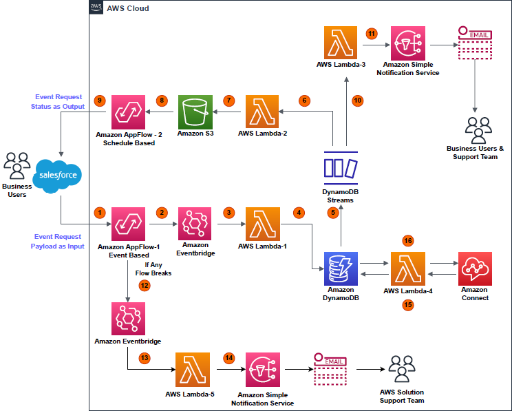
In this blog post, we demonstrate how to integrate Salesforce Lightning with Amazon DynamoDB by using Amazon AppFlow and Amazon EventBridge services bi-directionally. This is an event-driven, serverless-based microservice, allowing Salesforce users to update configuration data stored in DynamoDB tables without giving AWS account access from AWS Command Line Interface or AWS Management Console.

This architecture describes a contact center application that utilizes DynamoDB database to store configuration data, including holiday data, across different global regions. Updating this data in a table is a manual process, which includes creating a support ticket and waiting for completion of the support request. The architecture herein allows authorized business users to update the configuration data in DynamoDB directly from the Salesforce screen and not relying on manual update process.

Solution overview

As demonstrated in Figure 1, Amazon AppFlow consumes events payload from salesforce and Lambda updates the DynamoDB table after processing the payload. In parallel, a scheduled based flow sends response back to salesforce object as a notification and sends a SNS email notification to users. Contact center application (Amazon Connect) reads data from DynamoDB table.

Architecture overview

Figure 1. Architecture overview

  1. Event (data add or delete) occurring on a particular object in Salesforce is captured by Amazon AppFlow (event-based flow); event payload displays as “Input” in AWS environment.
  2. An EventBridge bus receives the “Input” payload.
  3. The EventBridge bus triggers the AWS Lambda (Lambda-1).
  4. Lambda-1 processes the “Input” payload, then performs a write operation (data add or delete) on a DynamoDB table.
  5. A write operation on the table triggers DynamoDB streams.
  6. DynamoDB stream triggers Lambda (Lambda-2).
  7. Lambda-2 processes the payload from DynamoDB streams. It saves the results in .csv file format, with a “Success” or “Fail” flag. This .csv file is uploaded to an S3 bucket.
  8. A second flow (schedule-based) is configured in Amazon AppFlow. This reads the S3 bucket at a regular interval of time to find new .csv files created by Lambda-2.
  9. A schedule-based flow transfers the .csv file data as an event-status output to the Salesforce object, notifying the user that their event has been successfully handled in DynamoDB table.
  10. In parallel, DynamoDB streams trigger Lambda (Lambda-3), which processes the payload and initiates an Amazon Simple Notification Service (Amazon SNS) notification based on the status of the event request.
  11. Amazon SNS sends an email to the user detailing that the event created in the Salesforce object was successfully completed in DynamoDB table.
  12. If any of the two flows break due to any unforeseen events, their statuses are instantly captured and streamed to an EventBridge bus.
  13. The EventBridge bus triggers Lambda (Lambda-5).
  14. Lambda-5 tries to analyze the error causing failure and tries to get the flow to a working state again. If Lambda-5 fails, it initiates an Amazon SNS email to the solution support team to manually fix the Amazon AppFlow error and get the solution active again.
  15. Meanwhile, whenever an Amazon Connect contact center receives a call, it triggers Lambda (Lambda-4), which holds read-only access to DynamoDB table.
  16. Lambda-4 fetches the data stored by Lambda-1 in DynamoDB table and provides that data to a contact center in Amazon Connect.

Prerequisites

  • An AWS account with permissions to access all the required
  • An active Salesforce account with administration-level permissions set
  • Python 3.X version setup for developing Lambda-1 to -5

Implementation and development

1. Development steps on the Salesforce end

Note: We recommend working with a Salesforce expert. These steps can help initiate the development from Salesforce end.

a. Use the Platform Event feature to allow the data flow from Salesforce environment to AWS environment and then back to Salesforce from AWS environment using Amazon AppFlow.
b. Salesforce Connected Apps and web server flow used for integrating Amazon AppFlow with Salesforce.
c. New permissions set and new integration users are created to restrict the access to custom object.

2. Development steps on the AWS end

a. Create a new connection in Amazon AppFlow with “Salesforce” as the source
The “Client ID” and “Client Secret” of Salesforce Managed Connected App are stored in AWS Secrets Manager, which is encrypted by custom keys generated in AWS Key Management Service.

To setup an Amazon AppFlow connection with Salesforce, a stand-alone Lambda function is created using Python Boto3 API. This creates a connection in Amazon AppFlow using the “Client ID” and “Client Secret” of Salesforce connected app.

For more details regarding setting up the Salesforce connection in Amazon AppFlow, refer to the Amazon AppFlow User Guide.

b. Create new event-based input flow in Amazon AppFlow, using Salesforce as the source with the newly created connection
Select the “Salesforce events” option as per the business use case. For representation in this blog, “Telephony” is chosen as salesforce events. Select Amazon EventBridge as the destination. Create new “partner event source” for successful creation of input flow, as in Figure 2.

Configure an event-based flow in Amazon AppFlow

Figure 2. Configure an event-based flow in Amazon AppFlow

c. Handling large size input flow event payloads
Post successful creation of “Partner event source”, specify the S3 bucket for events that are larger than 256 KB, Amazon AppFlow sends a URL of the S3 object to the event bus instead of the event payload.

d. Configuring details for input flow
Select trigger pattern of input flow as “Run flow on event”, as shown in Figure 3.

Trigger pattern for creating input flow

Figure 3. Trigger pattern for creating input flow

As displayed in Figure 4, we can configure data field mapping, validation rules, and filters with Amazon AppFlow. This enables us to enrich and modify event data before it is sent to the event bus. Post this, input flow create action is complete.

Mapping Salesforce object fields with Amazon EventBridge bus

Figure 4. Mapping Salesforce object fields with Amazon EventBridge bus

e. Associating Amazon AppFlow generated partner event source with the event bus in the Amazon EventBridge dashboard
Before activating the flow, access the Amazon EventBridge console to associate the AppFlow generated partner-event-source with the event bus (Figure 5).

Associating input flow partner event source with the Amazon EventBridge bus

Figure 5. Associating input flow partner event source with the Amazon EventBridge bus

f. Post Amazon EventBridge bus association, activate the input flow
After associating the bus with input flow, navigate back to Amazon AppFlow console and click the “Activate flow” button for the input flow. Once active, input flow is ready to consume the event payload from Salesforce.

g. Amazon EventBridge bus triggering Lambda function
The EventBridge bus receives an event payload from the input flow and triggers Lambda (Lambda-1) to process that raw event payload and write the output results in a designated DynamoDB table. A sample of event input payload is in Figure 6. This payload content depends on the use case for which developer is working.

Input event payload sample from Salesforce

Figure 6. Input event payload sample from Salesforce

Lambda-1 adds the record-ID in the DynamoDB table, which is a unique event ID for each Salesforce event as shown in Figure 7.

Data added in Amazon DynamoDB table by Lambda-1

Figure 7. Data added in Amazon DynamoDB table by Lambda-1

h. Configuring DynamoDB streams
Within “Export and Streams” option in the DynamoDB table, enable the “DynamoDB stream details” and in the trigger section click on “Create trigger” option and select  Lambda-2 and Lambda -3, as detailed in Figure 8.

Configuring Amazon DynamoDB streams

Figure 8. Configuring Amazon DynamoDB streams

Lambda-2 stores the event output results and a success flag value in a .csv file that is created for every unique event; the .csv file is uploaded to an S3 bucket with the file name structure “Salesforce event recorded-event action-timestamp.csv”. For example:

Example 1: “abcd1234-event-created- 2022-05-19-11_23_51.csv” (data added)
Example 2: “abcd1234-event-deleted- 2022-05-19-11_24_50.csv” (data deleted)

i. Create new schedule-based flow (output flow) in Amazon AppFlow
The source is the S3 bucket folder where the .csv file is uploaded by Lambda-2. Select the destination as “Salesforce”, and choose the Salesforce object that is used to create the input flow (Figure 9). Revisit Step b for reference.

Configuring a schedule-based output flow

Figure 9. Configuring a schedule-based output flow

Output flow sends a response back to the same Salesforce object from which data addition/deletion event request was made. This confirms to the user that a data addition/deletion event created in Salesforce was successfully invoked in Dynamo DB table as well.

j. Error handling in output flow
In case output flow fails to write the response back to the Salesforce object, choose the option “Stop the current flow run”.

k. Configuring output flow as a run-on schedule
Output flow is a schedule-based flow that runs at specific time. Within the flow trigger window, select “Run flow on schedule”. Update the other fields, such as “Repeats”, “Every”, “Start date”, and “Starting at” per your specific needs. Within “Transfer mode”, select “Incremental transfer”. Refer to Figure 10.

Trigger pattern for schedule-based output flow

Figure 10. Trigger pattern for schedule-based output flow

l. Amazon AppFlow to Salesforce object mapping for output flow
Select Mapping method as “Manually map fields” and Destination record preference as “Upsert records”, as in Figure 11.

Output Flow will update the event record status in the Salesforce object, with success status flag value in the .csv file based on the unique “Record ID” that every Salesforce event payload contains. Once the field mapping is completed, output flow is active.

Manually mapping data fields with Salesforce

Figure 11. Manually mapping data fields with Salesforce

m. Real-time monitoring and failure handling
In case input/output flow breaks for unforeseen reasons, a rule is configured in EventBridge bus console that invokes Lambda (Lambda-5). Lambda-5 tries to handle the error and reactivate the flow. In case this action fails, Lambda sends an Amazon SNS email to the solution support team informing of the failure in Amazon AppFlow and the cause.

n. Integrating DynamoDB with Amazon Connect
Lambda (Lambda-4) is configured with contact center in Amazon Connect. As the call comes to contact center, Lambda-4 fetches the relevant data from the DynamoDB table. Amazon Connect operates per this data.

Cleanup

To avoid incurring future charges, delete any AWS resources that are no longer needed.

Conclusion

This post demonstrates the approach for developing an event-driven, serverless application that integrates DynamoDB with Salesforce using Amazon AppFlow bi-directionally. The contact center is based in Amazon Connect and functions dependent on the real-time data in a DynamoDB table—without manual intervention. The manual process can take a minimum of 24 hours, but the same action can be automatically completed using a self-service, UI-based form in the user’s Salesforce account.

This solution can be tailored depending on the business or technical requirement, differing how the data is consumed by multiple AWS services.

Git’s Database Internals III: File History Queries (GitHub blog)

Post Syndicated from original https://lwn.net/Articles/906604/

The GitHub blog series on how the Git database works continues with this
look at file-history queries
.

If these history modes usually have the same output, then why
wouldn’t we always use --full-history
--simplify-merges? The reason is performance. Not only
does simplified history speed up the query by skipping a large
portion of commits, it also allows iterative output. The simplified
history can output portions of the history without walking the
entire history. By contrast, the --simplify-merges algorithm is
defined recursively starting at commits with no parents. Git cannot
output a single result until walking all reachable commits and
computing their diffs on the input path. This can be extremely slow
for large repositories.

High-School Graduation Prank Hack

Post Syndicated from Bruce Schneier original https://www.schneier.com/blog/archives/2022/08/high-school-graduation-prank-hack.html

This is a fun story, detailing the hack a group of high school students perpetrated against an Illinois school district, hacking 500 screens across a bunch of schools.

During the process, the group broke into the school’s IT systems; repurposed software used to monitor students’ computers; discovered a new vulnerability (and reported it); wrote their own scripts; secretly tested their system at night; and managed to avoid detection in the school’s network. Many of the techniques were not sophisticated, but they were pretty much all illegal.

It has a happy ending: no one was prosecuted.

A spokesperson for the D214 school district tells WIRED they can confirm the events in Duong’s blog post happened. They say the district does not condone hacking and the “incident highlights the importance of the extensive cybersecurity learning opportunities the District offers to students.”

“The District views this incident as a penetration test, and the students involved presented the data in a professional manner,” the spokesperson says, adding that its tech team has made changes to avoid anything similar happening again in the future.

The school also invited the students to a debrief, asking them to explain what they had done. “We were kind of scared at the idea of doing the debrief because we have to join a Zoom call, potentially with personally identifiable information,” Duong says. Eventually, he decided to use his real name, while other members created anonymous accounts. During the call, Duong says, they talked through the hack and he provided more details on ways the school could secure its system.

EDITED TO ADD (9/13): Here’s Minh Duong’s Defcon slides. You can see the table of contents of their report on page 59, and the school’s response on page 60.

Git’s database internals III: file history queries

Post Syndicated from Derrick Stolee original https://github.blog/2022-08-31-gits-database-internals-iii-file-history-queries/

This week, we are exploring Git’s internals with the following concept in mind:

Git is the distributed database at the core of your engineering system.

Before making a change to a large software system, it can be critical to understand the reasons why the code is in its current form. Looking at commit messages alone is insufficient for this discovery, and instead it is important to find the changes that modified a specific file or certain lines in that file. Git’s file history commands help users find these important points in time where changes were introduced.

Today, let’s dig into these different file history commands and consider them as a set of queries. We will learn how Git optimizes these queries based on the typical structure of file history and how merges work most of the time. Some additional history options may be required to discover what happened in certain special cases, such as using cherry-picks across multiple branches or mistakenly resolving merge conflicts incorrectly. Further, we will see some specialized data structures that accelerate these queries as repositories grow.

git log as file history

The primary way to discover which commits recently changed a file is to use git log -- <path>. This shows commits where their parent has a different Git object at <path>, but there are some subtleties as to which commits are shown, exactly.

One thing to keep in mind with file history queries is that the commit graph structure is still important. It is possible for two changes to happen in parallel and then be connected to the trunk through a merge. To help clarify what is happening with these queries, all examples in this section will assume that the --graph and --oneline options are also specified. The --graph option shows the relationships between commits and in particular will show when two commits are parallel to each other in the history. It also avoids interleaving two parallel sequences of commits that happen to have been created at the same time. I personally recommend that you use --graph whenever using these history walks.

The most important thing to remember is that commits are snapshots, not diffs. For a quick refresher on how we represent Git objects, see the key below.

A key to how different git objects are represented. A green circle represents a commit; a blue triangle represents a tree; and a red box represents a blob.

Git needs to dynamically compute the difference between two commits to see if <path> was changed. This means that Git loads the root trees for those two commits, then compares their tree entry for the first directory of <path> and compares the object ID found in each. This comparison is done recursively until equal object IDs are found (no difference) or all parts of <path> are walked and we find the two different objects at <path> for the two commits.

Image of two Git root trees, representing how Git dynamically computes the difference between two commits.

If we find equality during this process, we say that the two commits are treesame on this path.

For a commit with only one parent, we say that commit is interesting if it is not treesame. This is a natural idea, since this matches the only meaningful diff we could compute for that commit.

Similarly, a merge commit is considered interesting if it is not treesame to any of its parents. The figure below shows a number of interesting commits for a given path based on these treesame relationships.

Figure showing a number of interesting commits for a given path based on these treesame relationships.

In the case of an uninteresting merge commit where there is at least one treesame parent, Git makes different decisions based on the history query type.

Simplified history

By default, git log -- <path> shows the simplified history of <path>. This is defined in the git log documentation, but I’ll present an alternative definition here.

When the simplified history mode encounters a merge commit, it compares the merge commit to each parent in order. If Git finds a treesame parent, then it stops computing diffs at the current merge, marks the merge as uninteresting, and moves on to that parent. If all parents are not treesame, then Git marks the merge as interesting and adds all parents to the walk.

For a path that is not changed very often, almost every merge commit will be treesame to its first parent. This allows Git to skip checking all of the commits made reachable by merges that did not “introduce” a change to the trunk. When a topic branch is merged into the trunk, the new merge commit rarely has any merge conflicts, so it will be treesame to its second parent for all the files that were changed in that topic. The merge would then not be treesame to its first parent on any of these paths.

Figure representing how a merge commit is compared to each parent in order to determine whether it should be marked as interesting.

In the case that the merge commit is different from all of its parents on the path, then the merge is marked as interesting and all parents are added to the walk. This happens frequently when the path is a directory that has different sets of files change, but can also happen if the same file is modified by parallel changes and conflicts were resolved during the merge.

Here is an example query where two parallel topics both modified files inside the src/ directory:

$ git log --graph --oneline -- src/
*   80423fa Merge pull request #800 from ...
|\
| * 9313670 build(deps): bump Newtonsoft.Json in /src/shared/Core
* | 47ba58f diagnose: don't await Git exit on config list
|/
* 5637aa9 macos build: use runtime instead of osx-x64
* 7a99cc0 Fixes typo in Mac dist script

Note that the merge commits with a treesame parent are marked as uninteresting, even if they are different to their first parent. This means that the merge commit will not appear in the file history, even if it is responsible for introducing that change into the commit history. You can add the –show-pulls option to git log to make it output the merge commits that are different to their first parent. This can be particularly helpful if you are trying to also track which pull request was involved in that change.

Here is the output for the previous example, except that --show-pulls is added. Notice the additional “Merge pull request…” lines:

$ git log --graph --oneline --show-pulls -- src/
*   80423fa Merge pull request #800 from ...
|\
| * 9313670 build(deps): bump Newtonsoft.Json in /src/shared/Core
* | 77f7922 Merge pull request #804 from ...
* | 47ba58f diagnose: don't await Git exit on config list
|/
* b83bf02 Merge pull request #788 from ...
* 5637aa9 macos build: use runtime instead of osx-x64
* cf5a693 Merge pull request #778 from ...
* 7a99cc0 Fixes typo in Mac dist script

While this logic to skip huge chunks of history may seem confusing at first, it is a critical performance feature. It allows skipping commits that did not contribute to the latest version of the file. This works almost all of the time, but it is important to know some of the reasons why commits that might be interesting would be skipped by the simplified history mode.

Reverted Changes. Sometimes a pull request changes a file in its first version, but review feedback finds a different way to solve the problem without changing the file. The author might remove the changes to that file within their branch, but really has at least two commits editing the file. The end result makes no changes to the file since one commit reverts the previous changes. When that topic is merged, the merge commit is treesame to its first parent on that path and the topic branch is skipped.

Cherry-picks. Some bug fixes are critical to apply in multiple places, such as maintenance branches to solve security issues. If a commit is cherry-picked in multiple places, then it can look like “the same change” is happening in several parallel branches. If those branches eventually merge, they might merge automatically without conflict because all of the tips agree on the file contents. Thus, the simplified history walk will choose only one of these branches to walk and will discover one of the cherry-picks but not the others.

The previous two reasons are common but mostly harmless reasons why a commit could be skipped during simplified history. As someone who has worked on Git for several years, I can attest that the most common reason someone asks “what happened to my change?” is because of the more difficult third reason:

Merge conflict resolution. When resolving a merge, it is possible to make any number of mistakes. In particular, a common case is that someone gets confused and takes all of their changes and drops all changes from the other side of the merge. When this happens, simplified history works against us because Git sees a treesame parent and ignores the other side that had meaningful changes that were dropped by the merge conflict resolution.

These kinds of merge resolution issues are confusing on first glance, but we can use other history modes to discover what happened.

Full history

The --full-history mode changes from the simplified history mode by walking every commit in the history, regardless of treesame parents on merge commits. A merge commit is marked as interesting if there is at least one parent that is different at the path.

When used with --graph, Git performs parent rewriting to connect the parent links to the next interesting commit reachable from that parent. While the --full-history mode is sure to show all of the possible changes to the path, it is overly noisy. Here is the same repository used in the previous examples, but with --full-history we see many more merge commits:

$ git log --graph --oneline --full-history -- src/
*   5d869d9 Merge pull request #806 from ...
|\
* \   80423fa Merge pull request #800 from ...
|\ \
| |/
|/|
| * 9313670 build(deps): bump Newtonsoft.Json in /src/shared/Core
* |   77f7922 Merge pull request #804 from ...
|\ \
| * | 47ba58f diagnose: don't await Git exit on config list
* | | 162d657 Merge pull request #803 from ...
|/ /
* / 10935fb Merge pull request #700 from ...
|/
*   2d79a03 Merge pull request #797 from ...
|\
* | e209b3d Merge pull request #790 from ...
|/
*   b83bf02 Merge pull request #788 from ...
|\
| * 5637aa9 macos build: use runtime instead of osx-x64

Notice that these new merge commits have a second parent that wraps around and links back into the main history line. This is because that merge brought in a topic branch that did not change the src/ directory, but the first parent of the merge had some changes to the src/ directory relative to the base of the topic branch.

In this way, --full-history will show merges that bring in a topic branch whose history goes “around” meaningful changes. In a large repository, this noise can be so much that it is near impossible to find the important changes you are looking for.

The next history mode was invented to remove this extra noise.

Full history with simplified merges

In addition to --full-history, you can add the --simplify-merges option. This mode performs extra smoothing on the output of the --full-history mode, specifically dropping merge commits unless they actually are important for showing meaningful changes.

Recall from the --full-history example that some merge commits rewrote the second parent to be along the first-parent history. The --simplify-merges option starts by removing those parent connections and instead showing the merge as having a single parent. Then, Git inspects that commit as if it had a single parent from the beginning. If it is treesame to its only parent then that commit is removed. Git then rewrites any connections to that commit as going to its parent instead. This process continues until all simplifications are made, then the resulting history graph is shown.

$ git log --graph --oneline --full-history --simplify-merges -- src/
*   80423fa Merge pull request #800 from ...
|\
| * 9313670 build(deps): bump Newtonsoft.Json in /src/shared/Core
* | 47ba58f diagnose: don't await Git exit on config list
|/
* 5637aa9 macos build: use runtime instead of osx-x64
* 7a99cc0 Fixes typo in Mac dist script

Notice that this history is exactly the same as the simplified history example for this query. That is intentional: these should be the same results unless there really was an interesting change that was skipped.

If these history modes usually have the same output, then why wouldn’t we always use --full-history --simplify-merges? The reason is performance. Not only does simplified history speed up the query by skipping a large portion of commits, it also allows iterative output. The simplified history can output portions of the history without walking the entire history. By contrast, the --simplify-merges algorithm is defined recursively starting at commits with no parents. Git cannot output a single result until walking all reachable commits and computing their diffs on the input path. This can be extremely slow for large repositories.

One common complaint I have heard from Git users is “Git lost my change!” This typically takes the form where a developer knows that they merged in a commit that updated a file, but that change is no longer in the tip of that branch and running git log -- <path> does not show the commit they wrote! This kind of problem is due to file history simplification working as designed and skipping that commit, but it’s because someone created a faulty merge commit that is causing this unexpected behavior. If there is any chance that Git is skipping a commit that you know changed a file, then try to use --full-history with --simplify-merges.

To demonstrate, I took the previous example repository and created a branch that improperly resolved a merge to ignore valid changes that already existed in the trunk. Look carefully at the difference between the two history modes:

$ git log --graph --oneline -- src
* 5637aa9 macos build: use runtime instead of osx-x64
* 7a99cc0 Fixes typo in Mac dist script

$ git log --graph --oneline --full-history --simplify-merges -- src
*   7da271b Update with latest trunk
|\
| *   80423fa Merge pull request #800 from ...
| |\
| | * 9313670 build(deps): bump Newtonsoft.Json in /src/shared/Core
* | | 0b408b0 Resolve merge conflicts
|\| |
| |/
|/|
| * 47ba58f diagnose: don't await Git exit on config list
|/
* 5637aa9 macos build: use runtime instead of osx-x64
* 7a99cc0 Fixes typo in Mac dist script

When the actual history is shown, you can see that I created two “bad” merge commits: 7da271b Update with latest trunk and 0b408b0 Resolve merge conflicts. These both set the src directory equal to their first parents instead of allowing the merge to take the changes from both sides.

This history mode is a good tool to have in your arsenal.

Unfortunately, --full-history with --simplify-merges remains an expensive operation and I do not recommend using it by default. There remains no way to perform merge simplification without exploring the entire commit graph, even with the generation numbers discussed in part II. This remains an open problem, so if you have ideas about how to speed up this operation, then please bring those ideas to the Git developer community! I, for one, will be particularly interested!

Other history queries

Now that we’ve gone deep on the query modes for git log -- <path>, let’s consider a few other file history queries that shift the formula slightly in their own ways.

git log -L

The git log -L option allows specifying a portion of a file instead of an entire file. This helps you focus your history query to a specific function or set of lines. There are two main ways to use it:

  1. git log -L<from>,<to>:<path>: In the file at <path> show any changes in the lines between <from> and <to>.
  2. git log -L:<identifier>:<path>: In the file at <path>, find the code associated with <identifier> and show any changes to those lines. Usually, <identifier> is a function name, but it can also refer to a class or struct.

The -L mode modifies the definition of “treesame” to also consider two versions of the file to be the same if they have the same content at these lines. Importantly, Git will track how the line numbers change as the line content stays the same, but other changes to earlier lines might add or delete lines to the file outside of this range. After that definition of treesame is updated, the history walk is the same as in the simplified history mode.

In this way, the -L mode is more expensive because it needs to compute blob content diffs instead of only comparing object IDs. However, that performance difference can be worthwhile, as it reduces your time spent reading changes to the file that are not important to the section of the file you are reading.

git blame and git annotate

While git log will show all the commits that have changed a given file, the git blame and git annotate commands show the commits that most-recently changed each line of the file. The only difference between the commands is the output style.

To compute these most-recent changes, Git tracks each line in a similar way as it does for git log -L, but then drops the line from consideration once it has found a commit that changed that line.

Speeding up file history queries

The previous sections detailed the types of file history queries available in Git. These queries are similar to the commit history queries from part II in that it helps to walk the commits more quickly. However, file history queries spend a significant amount of time testing treesame relationships by computing diffs.

Recall from part I that we can navigate to the Git object specified by a path at a given commit by following a sequence of object links:

  • First, the commit has a root tree object ID that points to a tree object. The commit-graph file speeds this up slightly by including the root tree inside the commit-graph file instead of needing to parse the commit object directly.
  • Next, for each directory component in the path, Git parses a tree to find the matching tree entry and discovers the object ID of the next tree in the list.
  • Finally, the last tree entry points to the object ID for the object at the path. This could be a tree or a blob object.

The git log -L and git blame queries go an additional step further by computing a content diff of two blobs. We will not focus on this part right now, because this only happens if the blobs are already different.

Structuring repositories for fast history queries

Git spends most of its time parsing trees to satisfy these file history queries. There are a few different dimensions in the structure of the repository that can affect how much time is spent parsing trees:

  1. Tree depth: The number of directories required to reach the specified path means that more trees need to be parsed before finding the object ID for that path. For example, Java namespaces are tied to the directory structure of the source files, so the tree depth tends to be high in these repositories.
  2. Adjacent changes: When comparing two commits at a given path, Git can walk both sides of the comparison at the same time. If two tree entries point to the same object ID at any point along the list of trees, then Git can stop parsing trees and determine the commits are treesame at the path. This happens less frequently if the path is in a directory full of other files that are changed often. For example, a README file for a subproject might be rarely changed, but lives next to the code for that project that changes frequently.

If you are making choices to structure your repository, you might notice that these two dimensions are competing with each other. If you try to reduce the tree depth by using wider directory structures, then you will create more frequent adjacent changes. In reality, a middle ground is best between the two extremes of a very wide or very deep repository.

The other way your repository structure can change the performance of file history queries is actually in the commit history itself. Some repositories require a linear history through rebases or squash-merges. These repositories do not gain any performance benefits from the commit-skipping feature of simplified file history. On the other hand, a linear history will have the exact same history output for all of the history modes, so there is no need to use the advanced modes.

Luckily, Git has a feature that can speed up these file history queries regardless of the repository shape.

Changed-path Bloom filters

To speed up file history queries, Git has an optional query index that allows it to skip parsing trees in the vast majority of cases.

The changed path Bloom filters index stores a data structure called a Bloom filter for every commit. This index is stored in the commit-graph file, so you can compute it yourself using the git commit-graph write --reachable --changed-paths command. Once the changed-path Bloom filters are enabled in your commit-graph, all future writes will update them. This includes the commit-graph writes done by background maintenance enabled by git maintenance start.

A commit’s Bloom filter is a probabilistic set. It stores the information for each path changed between the first parent and that commit. Instead of storing those paths as a list, the Bloom filter uses hash algorithms to flip a set of bits that look random, but are predictable for each input path.

This Bloom filter allows us to ask the question: Is a given path treesame between the first parent and this commit? The answer can be one of two options:

  • Yes, probably different. In this case, we don’t know for sure that the path is different, so we need to parse trees to compute the diff.
  • No, definitely treesame. In this case, we can trust the filter and continue along the first-parent history without parsing any trees.

The parameters of the Bloom filter are configured in such a way that a random treesame path has a 98% likelihood of being reported as definitely treesame by the filter.

While running git log -- <path>, Git is in simplified history mode and checks the first parent of each commit to see if it is treesame. If the changed-path Bloom filter reports that the commit is treesame, then Git ignores the other parents and moves to the next commit without parsing any trees! If <path> is infrequently changed, then almost all commits will be treesame to their first parents for <path> and the Bloom filters can save 98% of the tree-parsing time!

It is reasonable to consider the overhead of checking the Bloom filters. Fortunately, the filters use hash algorithms in such a way that it is possible to hash the input <path> value into a short list of integers once at the start of the query. The remaining effort is to load the filter from the commit-graph file, modulo those integers based on the size of the filter, then check if certain bits are set in the filter. In this way, a single key is being tested against multiple filters, which is a bit unusual compared to the typical application of Bloom filters.

Git also takes advantage of the directory structure of <path>. For example, if the path is given as A/B/C/d.txt, then any commit that changed this path also changed A, A/B, and A/B/C. All of these strings are stored in the changed-path Bloom filter. Thus, we can reduce the number of false positives by testing all of these paths against each filter. If any of these paths is reported as treesame, then the full path must also be treesame.

To test the performance of these different modes, I found a deep path in the Linux kernel repository that was infrequently changed, but some adjacent files are frequently changed: drivers/gpu/drm/i915/TODO.txt.

Command No
commit-graph
No Bloom filters Bloom filters
git log -- <path> 1.03s 0.67s 0.18s
git log --full-history -- <path> 17.8s 11.0s 3.81s
git log --full-history --simplify-merges -- <path> 19.7s 13.3s 5.39s

For queries such as git log -L and git blame, the changed-path Bloom filters only prevent that initial treesame check. When there is a difference between two commits, the content-based diff algorithm still needs to do the same amount of work. This means the performance improvements are more modest for these queries.

For this example, I used a path that is changed slightly more frequently than the previous one, but in the same directory: drivers/gpu/drm/i915/Makefile.

Command No
commit-graph
No Bloom filters Bloom filters
git blame <path> 1.04s 0.82s 0.21s
git log -L100,110:<path> 9.67s 2.64s 1.38s

These performance gains are valuable for a normal user running Git commands in their terminal, but they are extremely important for Git hosting services such as GitHub that use these same Git history queries to power the web history interface. Computing the changed-path Bloom filters in advance can save thousands of CPU hours due to the frequency that users request this data from that centralized source.

Come back tomorrow for more!

Today, we went even deeper into Git’s internals and how its file history modes act as specialized queries into the commit history. Learning these advanced query types is similar to learning advanced language features of SQL such as different JOIN types. The commit-graph file again operated as a query index to accelerate these history queries.

In the next part of this blog series, we will explore how Git acts as a distributed database. Specifically, we will dig into how git fetch and git push help synchronize remote copies of a repository. The structure of the commit graph will be critical, but the cost of parsing trees will be even more immediate. We’ll talk about how reachability bitmaps can speed up some of these operations, but also explore some reasons why bitmaps are not always used.

I’ll also be speaking at Git Merge 2022 covering all five parts of this blog series, so I look forward to seeing you there!
The collective thoughts of the interwebz