Post Syndicated from Crosstalk Solutions original https://www.youtube.com/watch?v=VJ8gNDkwKYU
Will people stop caring if images are real or AI?
Post Syndicated from The Atlantic original https://www.youtube.com/shorts/pwmUdz2rUj8
Security updates for Tuesday
Post Syndicated from jzb original https://lwn.net/Articles/1067595/
Security updates have been issued by Debian (gdk-pixbuf, gst-plugins-bad1.0, and xdg-dbus-proxy), Fedora (chromium, deepin-image-viewer, dtk6gui, dtkgui, efl, elementary-photos, entangle, flatpak, freeimage, geeqie, gegl04, gthumb, ImageMagick, kf5-kimageformats, kf5-libkdcraw, kf6-kimageformats, kstars, libkdcraw, libpasraw, LibRaw, luminance-hdr, nomacs, OpenImageIO, OpenImageIO2.5, photoqt, python-cryptography, rawtherapee, shotwell, siril, swayimg, vips, and webkitgtk), Red Hat (firefox and podman), Slackware (libarchive), SUSE (expat, glibc, GraphicsMagick, libcap-devel, libpng16, libtpms, nodejs24, openssl-1_0_0, openssl-1_1, openssl-3, openvswitch, polkit, python-requests, python311-biopython, python312, python39, and tigervnc), and Ubuntu (corosync, kvmtool, libxml-parser-perl, linux-azure, linux-azure, linux-azure-6.17, linux-azure, linux-azure-6.8, policykit-1, redis, lua5.1, lua-cjson, lua-bitop, rustc, vim, and xdg-dbus-proxy).
THG Podcast – Counterfactuals: Tsushima
Post Syndicated from The History Guy: History Deserves to Be Remembered original https://www.youtube.com/watch?v=WZSW90SqHeE
Securing non-human identities: automated revocation, OAuth, and scoped permissions
Post Syndicated from Justin Hutchings original https://blog.cloudflare.com/improved-developer-security/
Agents let you build software faster than ever, but securing your environment and the code you write — from both mistakes and malice — takes real effort. Open Web Application Security Project (OWASP) details a number of risks present in agentic AI systems, including the risk of credential leaks, user impersonation, and elevation of privilege. These risks can result in extreme damage to your environments including denial of service, data loss, or data leaks — which can do untold financial and reputational damage.
This is an identity problem. In modern development, “identities” aren’t just people — they are the agents, scripts, and third-party tools that act on your behalf. To secure these non-human identities, you need to manage their entire lifecycle: ensuring their credentials (tokens) aren’t leaked, seeing which applications have access via OAuth, and narrowing their permissions using granular RBAC.
Today, we are introducing updates to address these needs: scannable tokens to protect your credentials, OAuth visibility to manage your principals, and resource-scoped RBAC to fine-tune your policies.
To secure the Internet in an era of autonomous agents, we have to rethink how we handle identity. Whether a request comes from a human developer or an AI agent, every interaction with an API relies on three core pillars:
-
The Principal (The Traveler): This is the identity itself — the “who.” It might be you logging in via OAuth, or a background agent using an API token to deploy code.
-
The Credential (The Passport): This is the proof of that identity. In this world, your API token is your passport. If it’s stolen or leaked, anyone can “wear” your identity.
-
The Policy (The Visa): This defines what that identity is allowed to do. Just because you have a valid passport doesn’t mean you have a visa to enter every country. A policy ensures that even a verified identity can only access the specific resources it needs.
When these three pillars aren’t managed together, security breaks down. You might have a valid Principal using a stolen Credential, or a legitimate identity with a Policy that is far too broad.
Agents and other third-party applications use API tokens to access the Cloudflare API. One of the simplest ways that we see people leaking their secrets is by accidentally pushing them to a public GitHub repository. GitGuardian reports that last year more than 28 million secrets were published to public GitHub repositories, and that AI is causing leaks to happen 5x faster than before.
If an API token is a digital passport, then leaking it on a public repository is like leaving your passport on a park bench. Anyone who finds it can impersonate that identity until the document is canceled. Our partnership with GitHub acts like a global “lost and found” for these credentials. By the time you realize your passport is missing, we’ve already identified the document, verified its authenticity via the checksum, and voided it to prevent misuse.
We’re partnering with several leading credential scanning tools to help proactively find your leaked tokens and revoke them before they could be used maliciously. We know it’s not a matter of if, but rather when, before you, an employee, or one of your agents makes a mistake and pushes a secret somewhere it shouldn’t be.
We’ve partnered with GitHub and are participating in their Secret Scanning program to find your tokens in both public and private repositories. If we are notified that a token has leaked to a public repository, we will automatically revoke the token to prevent it from being used maliciously. For private repositories, GitHub will notify you about any leaked Cloudflare tokens and you can clean these up.
We’ve shared the new token formats (below!) with GitHub, and they now scan for them on every commit. If they find something that looks like a leaked Cloudflare token, they verify the token is real (using the checksum), send us a webhook to revoke it, and then we notify you via email so you can generate a new one in Dashboard settings.
This means we plug the hole as soon as it’s found. By the time you realize you made a mistake, we’ve already fixed it.
We hope this is the kind of feature you don’t need to use, but our partners are on the lookout for leaks to help keep you secure.
Cloudflare One customers are also protected from these leaks. By configuring the Credentials and Secrets DLP profile, organizations can activate prevention everywhere a credential can travel:
-
Network Traffic (Cloudflare Gateway): Apply these entries to a policy to detect and block Cloudflare API tokens moving across your network. A token in a file upload, an outbound request, or a download is stopped before it reaches its destination.
-
Outbound Email (Cloudflare Email Security): Microsoft 365 customers can extend this same prevention to Outlook. The DLP Assist add-in scans messages before delivery, catching a token before it’s sent externally.
-
Data at Rest (Cloudflare CASB): Cloudflare’s Cloud Access Security Broker applies the same profile to scan files across connected SaaS applications, catching tokens saved or shared in Google Drive, OneDrive, Dropbox, and other integrated services.
The most novel exposure vector, though, is AI traffic. Cloudflare AI Gateway integrates with the same DLP profiles to scan and block both incoming prompts and outgoing AI model responses in real time.
The only way credential scanning works is if we meet you where you are, so we are working with several open source and commercial credential scanners to ensure you are protected no matter what secret scanner you use.
Until now, Cloudflare’s API tokens were pretty generic looking, so they were hard for credential scanners to identify with high confidence. These automated security tools scan your code repositories looking for exposed credentials like API keys, tokens or passwords. The “cf” prefix makes Cloudflare tokens instantly recognizable with greater confidence, and the checksum makes it easy for tools to statically validate them. Your existing tokens will continue to work, but every new token you generate will use the scannable format so it’s easily detected with high confidence.
|
Credential Type |
What it’s for |
New Format |
|
User API Key |
Legacy global API key tied to your user account (full access) |
cfk_[40 characters][checksum] |
|
User API Token |
Scoped token you create for specific permissions |
cfut_[40 characters][checksum] |
|
Account API Token |
Token owned by the account (not a specific user) |
cfat_[40 characters][checksum] |
If you have existing API tokens, you can roll the token to create a new, scannable API token. This is optional, but recommended to ensure that your tokens are easily discoverable in case they leak.
While API tokens are generally used by your own scripts and agents, OAuth is how you manage access for third-party platforms. Both require clear visibility to prevent unauthorized access and ensure you know exactly who — or what — has access to your data.
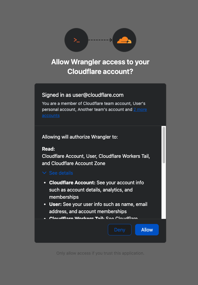
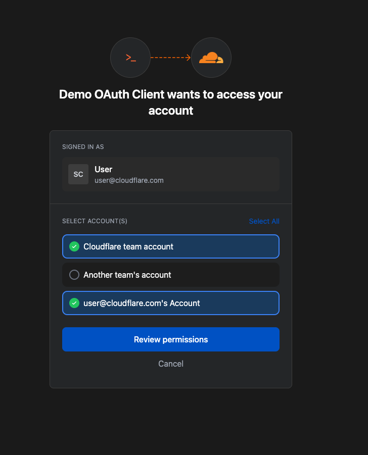
When you connect third-party applications like Wrangler to your Cloudflare Account using OAuth, you’re granting that application access to your account’s data. Over time, you may forget why you granted a third party application access to your Account in the first place. Previously, there was no central place to view & manage those applications. Starting today, there is.
Going forward, when a third party application requests access to your Cloudflare account, you’ll be able to review:
-
Which third-party application is requesting access, along with information about the application like Name, Logo, and the Publisher.
-
Which scopes the third-party application is requesting access to.
-
Which accounts to grant the third party application access to.
| Before | After |
|---|---|
 |
|
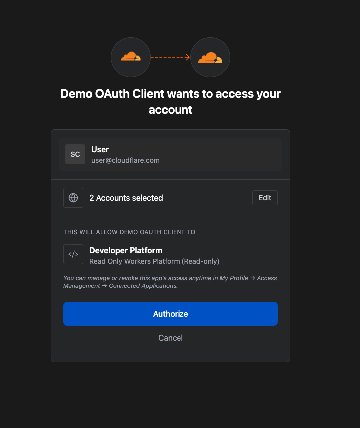
Not all applications require the same permissions; some only need to read data, others may need to make changes to your Account. Understanding these scopes before you grant access helps you maintain least-privilege.
We also added a Connected Applications experience so you can see which applications have access to which accounts, what scopes/permissions are associated with that application, and easily revoke that access as needed.
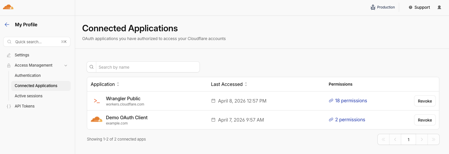
The OAuth consent and revocation improvements are available now. Check which apps currently have access to your accounts by visiting My Profile > Access Management > Connected Applications.
For developers building integrations with Cloudflare, keep an eye on the Cloudflare Changelog for more announcements around how you can register your own OAuth apps soon!
If the token is the passport, then resource-scoped permissions are the visas inside it. Having a valid passport gets you through the front door, but it shouldn’t give you access to every room in the building. By narrowing the scope to specific resources — like a single Load Balancer pool or a specific Gateway policy — you are ensuring that even if an identity is verified, it only has the “visa” to go where it’s strictly necessary.
Last year, we announced support for resource scoped permissions in Cloudflare’s role-based access control (RBAC) system for several of our Zero Trust products. This enables you to right size permissions for both users and agents to minimize security risks. We’ve expanded this capability to several new resources-level permissions. The resource scope is now supported for:
-
Access Applications
-
Access Identity Providers
-
Access Policies
-
Access Service Tokens
-
Access Targets
We’ve also completely overhauled the API Token creation experience, making it easier for customers to provision and manage Account API Tokens right from the Cloudflare Dashboard.

When you add a member to your Cloudflare account or create an API Token, you typically assign that principal a policy. A Permission Policy is what gives a principal permission to take an action, whether that’s managing Cloudflare One Access Applications, or DNS Records. Without a policy, a principal can authenticate, but they are unauthorized to do any actions within an account.
Policies are made up of three components: a Principal, a Role, and a Scope. The Principal is who or what you’re granting access to, whether that’s a human user, a Non-Human Identity (NHI) like an API Token, or increasingly, an Agent acting on behalf of a user. The Role defines what actions they’re permitted to take. The Scope determines where those permissions apply, and historically, that’s been restricted to the entire account, or individual zones.
We’re also expanding the role surface more broadly at both the Account & Zone level with the introduction of a number of new roles for many products.
-
Account scope
-
CDN Management
-
MCP Portals
-
Radar
-
Request Tracer
-
SSL/TLS Management
-
-
Zone scope
-
Analytics
-
Logpush
-
Page Rules
-
Security Center
-
Snippets
-
Zone Settings
-
The resource scope and all new account and zone-level roles are available today for all Cloudflare customers. You can assign account, zone, or resource-scoped policies through the Cloudflare Dashboard, the API, or Terraform.
For a full breakdown of all available roles and how scopes work, visit our roles and scope documentation.
These updates provide the granular building blocks needed for a true least-privilege architecture. By refining how we manage permissions and credentials, developers and enterprises can have greater confidence in their security posture across the users, apps, agents, and scripts that access Cloudflare. Least privilege isn’t a new concept, and for enterprises, it’s never been optional. Whether a human administrator is managing a zone or an agent is programmatically deploying a Worker, the expectation is the same, they should only be authorized to do the job it was given, and nothing else.
Following today’s announcement, we recommend customers:
-
Review your API tokens, and reissue with the new, scannable API tokens as soon as possible.
-
Review your authorized OAuth apps, and revoke any that you are no longer using
-
Review member & API Token permissions in your accounts and ensure that users are taking advantage of the new account, zone, or resource scoped permissions as needed to reduce your risk area.
Scaling MCP adoption: Our reference architecture for simpler, safer and cheaper enterprise deployments of MCP
Post Syndicated from Sharon Goldberg original https://blog.cloudflare.com/enterprise-mcp/
We at Cloudflare have aggressively adopted Model Context Protocol (MCP) as a core part of our AI strategy. This shift has moved well beyond our engineering organization, with employees across product, sales, marketing, and finance teams now using agentic workflows to drive efficiency in their daily tasks. But the adoption of agentic workflow with MCP is not without its security risks. These range from authorization sprawl, prompt injection, and supply chain risks. To secure this broad company-wide adoption, we have integrated a suite of security controls from both our Cloudflare One (SASE) platform and our Cloudflare Developer platform, allowing us to govern AI usage with MCP without slowing down our workforce.
In this blog we’ll walk through our own best practices for securing MCP workflows, by putting different parts of our platform together to create a unified security architecture for the era of autonomous AI. We’ll also share two new concepts that support enterprise MCP deployments:
-
We are launching Code Mode with MCP server portals, to drastically reduce token costs associated with MCP usage;
-
We describe how to use Cloudflare Gateway for Shadow MCP detection, to discover use of unauthorized remote MCP servers.
We also talk about how our organization approached deploying MCP, and how we built out our MCP security architecture using Cloudflare products including remote MCP servers, Cloudflare Access, MCP server portals and AI Gateway.
MCP is an open standard that enables developers to build a two-way connection between AI applications and the data sources they need to access. In this architecture, the MCP client is the integration point with the LLM or other AI agent, and the MCP server sits between the MCP client and the corporate resources.

The separation between MCP clients and MCP servers allows agents to autonomously pursue goals and take actions while maintaining a clear boundary between the AI (integrated at the MCP client) and the credentials and APIs of the corporate resource (integrated at the MCP server).
Our workforce at Cloudflare is constantly using MCP servers to access information in various internal resources, including our project management platform, our internal wiki, documentation and code management platforms, and more.
Very early on, we realized that locally-hosted MCP servers were a security liability. Local MCP server deployments may rely on unvetted software sources and versions, which increases the risk of supply chain attacks or tool injection attacks. They prevent IT and security administrators from administrating these servers, leaving it up to individual employees and developers to choose which MCP servers they want to run and how they want to keep them up to date. This is a losing game.

Instead, we have a centralized team at Cloudflare that manages our MCP server deployment across the enterprise. This team built a shared MCP platform inside our monorepo that provides governed infrastructure out of the box. When an employee wants to expose an internal resource via MCP, they first get approval from our AI governance team, and then they copy a template, write their tool definitions, and deploy, all the while inheriting default-deny write controls with audit logging, auto-generated CI/CD pipelines, and secrets management for free. This means standing up a new governed MCP server is minutes of scaffolding. The governance is baked into the platform itself, which is what allowed adoption to spread so quickly.
Our CI/CD pipeline deploys them as remote MCP servers on custom domains on Cloudflare’s developer platform. This gives us visibility into which MCPs servers are being used by our employees, while maintaining control over software sources. As an added bonus, every remote MCP server on the Cloudflare developer platform is automatically deployed across our global network of data centers, so MCP servers can be accessed by our employees with low latency, regardless of where they might be in the world.
Some of our MCP servers sit in front of public resources, like our Cloudflare documentation MCP server or Cloudflare Radar MCP server, and thus we want them to be accessible to anyone. But many of the MCP servers used by our workforce are sitting in front of our private corporate resources. These MCP servers require user authentication to ensure that they are off limits to everyone but authorized Cloudflare employees. To achieve this, our monorepo template for MCP servers integrates Cloudflare Access as the OAuth provider. Cloudflare Access secures login flows and issues access tokens to resources, while acting as an identity aggregator that verifies end user single-sign on (SSO), multifactor authentication (MFA), and a variety of contextual attributes such as IP addresses, location, or device certificates.

MCP server portals unify governance and control for all AI activity.
As the number of our remote MCP servers grew, we hit a new wall: discovery. We wanted to make it easy for every employee (especially those that are new to MCP) to find and work with all the MCP servers that are available to them. Our MCP server portals product provided a convenient solution. The employee simply connects their MCP client to the MCP server portal, and the portal immediately reveals every internal and third-party MCP servers they are authorized to use.
Beyond this, our MCP server portals provide centralized logging, consistent policy enforcement and data loss prevention (DLP guardrails). Our administrators can see who logged into what MCP portal and create DLP rules that prevent certain data, like personally identifiable data (PII), from being shared with certain MCP servers.
We can also create policies that control who has access to the portal itself, and what tools from each MCP server should be exposed. For example, we could set up one MCP server portal that is only accessible to employees that are part of our finance group that exposes just the read-only tools for the MCP server in front of our internal code repository. Meanwhile, a different MCP server portal, accessible only to employees on their corporate laptops that are in our engineering team, could expose more powerful read/write tools to our code repository MCP server.
An overview of our MCP server portal architecture is shown above. The portal supports both remote MCP servers hosted on Cloudflare, and third-party MCP servers hosted anywhere else. What makes this architecture uniquely performant is that all these security and networking components run on the same physical machine within our global network. When an employee’s request moves through the MCP server portal, a Cloudflare-hosted remote MCP server, and Cloudflare Access, their traffic never needs to leave the same physical machine.
After months of high-volume MCP deployments, we’ve paid out our fair share of tokens. We’ve also started to think most people are doing MCP wrong.
The standard approach to MCP requires defining a separate tool for every API operation that is exposed via an MCP server. But this static and exhaustive approach quickly exhausts an agent’s context window, especially for large platforms with thousands of endpoints.
We previously wrote about how we used server-side Code Mode to power Cloudflare’s MCP server, allowing us to expose the thousands of end-points in Cloudflare API while reducing token use by 99.9%. The Cloudflare MCP server exposes just two tools: a search tool lets the model write JavaScript to explore what’s available, and an execute tool lets it write JavaScript to call the tools it finds. The model discovers what it needs on demand, rather than receiving everything upfront.
We like this pattern so much, we had to make it available for everyone. So we have now launched the ability to use the “Code Mode” pattern with MCP server portals. Now you can front all of your MCP servers with a centralized portal that performs audit controls and progressive tool disclosure, in order to reduce token costs.
Here is how it works. Instead of exposing every tool definition to a client, all of your underlying MCP servers collapse into just two MCP portal tools: portal_codemode_search and portal_codemode_execute. The search tool gives the model access to a codemode.tools() function that returns all the tool definitions from every connected upstream MCP server. The model then writes JavaScript to filter and explore these definitions, finding exactly the tools it needs without every schema being loaded into context. The execute tool provides a codemode proxy object where each upstream tool is available as a callable function. The model writes JavaScript that calls these tools directly, chaining multiple operations, filtering results, and handling errors in code. All of this runs in a sandboxed environment on the MCP server portal powered by Dynamic Workers.
Here is an example of an agent that needs to find a Jira ticket and update it with information from Google Drive. It first searches for the right tools:
// portal_codemode_search
async () => {
 const tools = await codemode.tools();
 return tools
  .filter(t => t.name.includes("jira") || t.name.includes("drive"))
  .map(t => ({ name: t.name, params: Object.keys(t.inputSchema.properties || {}) }));
}
The model now knows the exact tool names and parameters it needs, without the full schemas of tools ever entering its context. It then writes a single execute call to chain the operations together:
// portal_codemode_execute
async () => {
 const tickets = await codemode.jira_search_jira_with_jql({
  jql: ‘project = BLOG AND status = “In Progress”’,
  fields: [“summary”, “description”]
 });
 const doc = await codemode.google_workspace_drive_get_content({
  fileId: “1aBcDeFgHiJk”
 });
 await codemode.jira_update_jira_ticket({
  issueKey: tickets[0].key,
  fields: { description: tickets[0].description + “\n\n” + doc.content }
 });
 return { updated: tickets[0].key };
}
This is just two tool calls. The first discovers what’s available, the second does the work. Without Code Mode, this same workflow would have required the model to receive the full schemas of every tool from both MCP servers upfront, and then make three separate tool invocations.
Let’s put the savings in perspective: when our internal MCP server portal is connected to just four of our internal MCP servers, it exposes 52 tools that consume approximately 9,400 tokens of context just for their definitions. With Code Mode enabled, those 52 tools collapse into 2 portal tools consuming roughly 600 tokens, a 94% reduction. And critically, this cost stays fixed. As we connect more MCP servers to the portal, the token cost of Code Mode doesn’t grow.
Code Mode can be activated on an MCP server portal by adding a query parameter to the URL. Instead of connecting to your portal over its usual URL (e.g. https://myportal.example.com/mcp), you attach ?codemode=search_and_execute to the URL (e.g. https://myportal.example.com/mcp?codemode=search_and_execute).
We aren’t done yet. We plug AI Gateway into our architecture by positioning it on the connection between the MCP client and the LLM. This allows us to quickly switch between various LLM providers (to prevent vendor lock-in) and to enforce cost controls (by limiting the number of tokens each employee can burn through). The full architecture is shown below.

Now that we’ve provided governed access to authorized MCP servers, let’s look into dealing with unauthorized MCP servers. We can perform shadow MCP discovery using Cloudflare Gateway. Cloudflare Gateway is our comprehensive secure web gateway that provides enterprise security teams with visibility and control over their employees’ Internet traffic.
We can use the Cloudflare Gateway API to perform a multi-layer scan to find remote MCP servers that are not being accessed via an MCP server portal. This is possible using a variety of existing Gateway and Data Loss Prevention (DLP) selectors, including:
-
Using the Gateway
httpHostselector to scan for-
known MCP server hostnames using (like mcp.stripe.com)
-
mcp.* subdomains using wildcard hostname patterns
-
-
Using the Gateway
httpRequestURIselector to scan for MCP-specific URL paths like /mcp and /mcp/sse -
Using DLP-based body inspection to find MCP traffic, even if that traffic uses URI that do not contain the telltale mentions of
mcporsse. Specifically, we use the fact that MCP uses JSON-RPC over HTTP, which means every request contains a “method” field with values like “tools/call”, “prompts/get”, or “initialize.” Here are some regex rules that can be used to detect MCP traffic in the HTTP body:
const DLP_REGEX_PATTERNS = [
  {
    name: "MCP Initialize Method",
    regex: '"method"\\s{0,5}:\\s{0,5}"initialize"',
  },
  {
    name: "MCP Tools Call",
    regex: '"method"\\s{0,5}:\\s{0,5}"tools/call"',
  },
  {
    name: "MCP Tools List",
    regex: '"method"\\s{0,5}:\\s{0,5}"tools/list"',
  },
  {
    name: "MCP Resources Read",
    regex: '"method"\\s{0,5}:\\s{0,5}"resources/read"',
  },
  {
    name: "MCP Resources List",
    regex: '"method"\\s{0,5}:\\s{0,5}"resources/list"',
  },
  {
    name: "MCP Prompts List",
    regex: '"method"\\s{0,5}:\\s{0,5}"prompts/(list|get)"',
  },
  {
    name: "MCP Sampling Create Message",
    regex: '"method"\\s{0,5}:\\s{0,5}"sampling/createMessage"',
  },
  {
    name: "MCP Protocol Version",
    regex: '"protocolVersion"\\s{0,5}:\\s{0,5}"202[4-9]',
  },
  {
    name: "MCP Notifications Initialized",
    regex: '"method"\\s{0,5}:\\s{0,5}"notifications/initialized"',
  },
  {
    name: "MCP Roots List",
    regex: '"method"\\s{0,5}:\\s{0,5}"roots/list"',
  },
];
The Gateway API supports additional automation. For example, one can use the custom DLP profile we defined above to block traffic, or redirect it, or just to log and inspect MCP payloads. Put this together, and Gateway can be used to provide comprehensive detection of unauthorized remote MCP servers accessed via an enterprise network.
For more information on how to build this out, see this tutorial.
So far, we’ve been focused on protecting our workforce’s access to our internal MCP servers. But, like many other organizations, we also have public-facing MCP servers that our customers can use to agentically administer and operate Cloudflare products. These MCP servers are hosted on Cloudflare’s developer platform. (You can find a list of individual MCPs for specific products here, or refer back to our new approach for providing more efficient access to the entire Cloudflare API using Code Mode.)
We believe that every organization should publish official, first-party MCP servers for their products. The alternative is that your customers source unvetted servers from public repositories where packages may contain dangerous trust assumptions, undisclosed data collection, and any range of unsanctioned behaviors. By publishing your own MCP servers, you control the code, update cadence, and security posture of the tools your customers use.
Since every remote MCP server is an HTTP endpoint, we can put it behind the Cloudflare Web Application Firewall (WAF). Customers can enable the AI Security for Apps feature within the WAF to automatically inspect inbound MCP traffic for prompt injection attempts, sensitive data leakage, and topic classification. Public facing MCPs are protected just as any other web API.
We hope our experience, products, and reference architectures will be useful to other organizations as they continue along their own journey towards broad enterprise-wide adoption of MCP.
We’ve secured our own MCP workflows by:
-
Offering our developers a templated framework for building and deploying remote MCP servers on our developer platform using Cloudflare Access for authentication
-
Ensuring secure, identity-based access to authorized MCP servers by connecting our entire workforce to MCP server portals
-
Controlling costs using AI Gateway to mediate access to the LLMs powering our workforce’s MCP clients, and using Code Mode in MCP server portals to reduce token consumption and context bloat
-
Discovering shadow MCP usage by Cloudflare Gateway
For organizations advancing on their own enterprise MCP journeys, we recommend starting by putting your existing remote and third-party MCP servers behind Cloudflare MCP server portals and enabling Code Mode to start benefitting for cheaper, safer and simpler enterprise deployments of MCP.
Acknowledgements: This reference architecture and blog represents this work of many people across many different roles and business units at Cloudflare. This is just a partial list of contributors: Ann Ming Samborski, Kate Reznykova, Mike Nomitch, James Royal, Liam Reese, Yumna Moazzam, Simon Thorpe, Rian van der Merwe, Rajesh Bhatia, Ayush Thakur, Gonzalo Chavarri, Maddy Onyehara, and Haley Campbell.
Managed OAuth for Access: make internal apps agent-ready in one click
Post Syndicated from Eduardo Gomes original https://blog.cloudflare.com/managed-oauth-for-access/
We have thousands of internal apps at Cloudflare. Some are things we’ve built ourselves, others are self-hosted instances of software built by others. They range from business-critical apps nearly every person uses, to side projects and prototypes.
All of these apps are protected by Cloudflare Access. But when we started using and building agents — particularly for uses beyond writing code — we hit a wall. People could access apps behind Access, but their agents couldn’t.
Access sits in front of internal apps. You define a policy, and then Access will send unauthenticated users to a login page to choose how to authenticate.

Example of a Cloudflare Access login page
This flow worked great for humans. But all agents could see was a redirect to a login page that they couldn’t act on.
Providing agents with access to internal app data is so vital that we immediately implemented a stopgap for our own internal use. We modified OpenCode’s web fetch tool such that for specific domains, it triggered the cloudflared CLI to open an authorization flow to fetch a JWT (JSON Web Token). By appending this token to requests, we enabled secure, immediate access to our internal ecosystem.
While this solution was a temporary answer to our own dilemma, today we’re retiring this workaround and fixing this problem for everyone. Now in open beta, every Access application supports managed OAuth. One click to enable it for an Access app, and agents that speak OAuth 2.0 can easily discover how to authenticate (RFC 9728), send the user through the auth flow, and receive back an authorization token (the same JWT from our initial solution).
Now, the flow works smoothly for both humans and agents. Cloudflare Access has a generous free tier. And building off our newly-introduced Organizations beta, you’ll soon be able to bridge identity providers across Cloudflare accounts too.
For a given internal app protected by Cloudflare Access, you enable managed OAuth in one click:
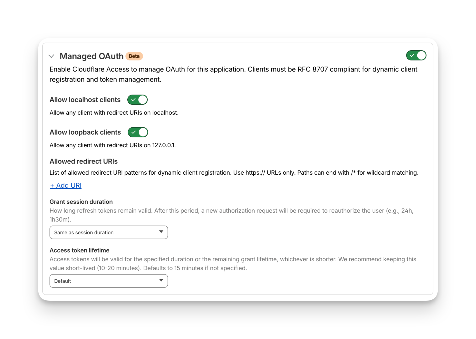
Once managed OAuth is enabled, Cloudflare Access acts as the authorization server. It returns the www-authenticate header, telling unauthorized agents where to look up information on how to get an authorization token. They find this at https://<your-app-domain>/.well-known/oauth-authorization-server. Equipped with that direction, agents can just follow OAuth standards:
-
The agent dynamically registers itself as a client (a process known as Dynamic Client Registration — RFC 7591),
-
The agent sends the human through a PKCE (Proof Key for Code Exchange) authorization flow (RFC 7636)
-
The human authorizes access, which grants a token to the agent that it can use to make authenticated requests on behalf of the user
Here’s what the authorization flow looks like:
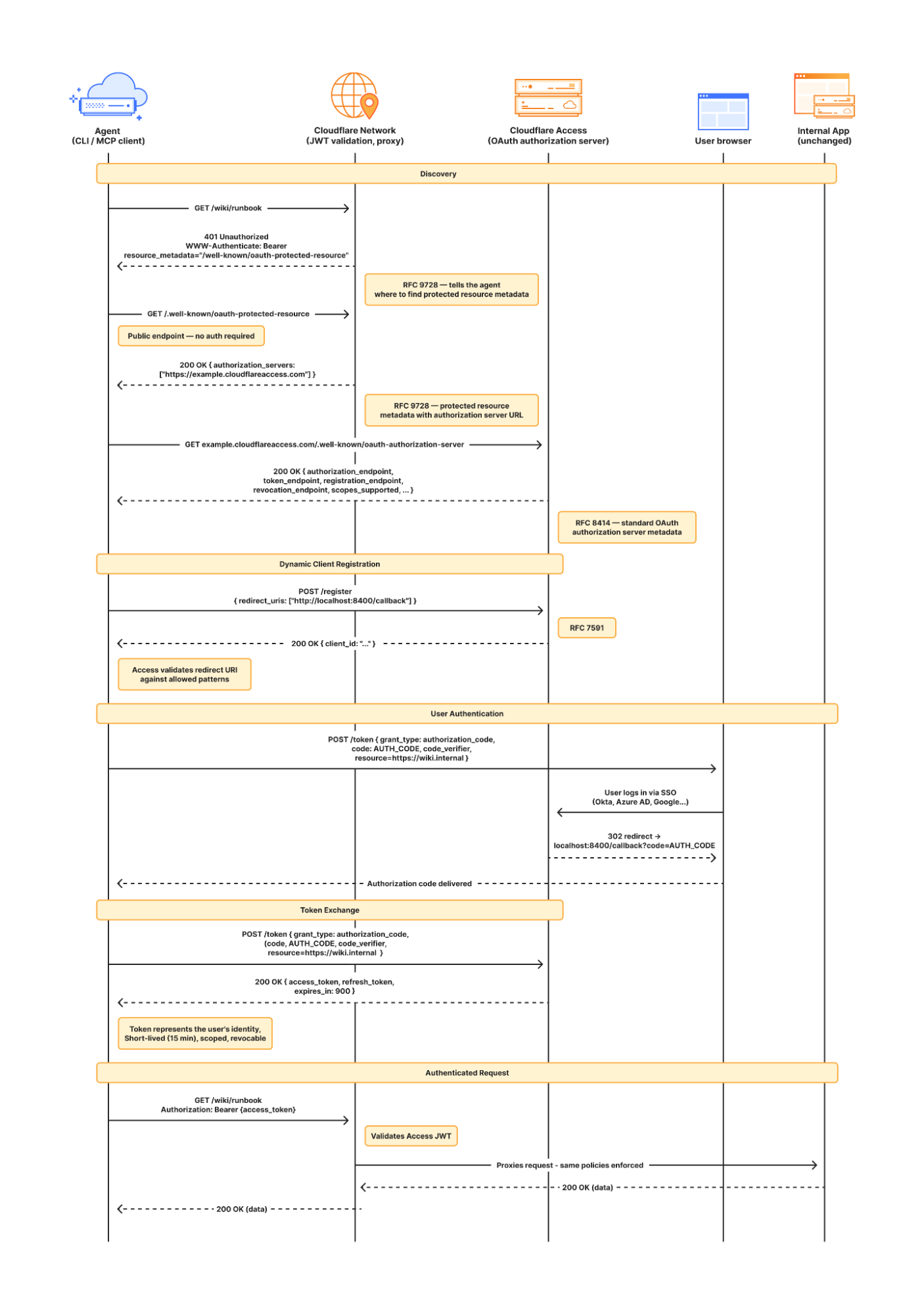
If this authorization flow looks familiar, that’s because it’s what the Model Context Protocol (MCP) uses. We originally built support for this into our MCP server portals product, which proxies and controls access to many MCP servers, to allow the portal to act as the OAuth server. Now, we’re bringing this to all Access apps so agents can access not only MCP servers that require authorization, but also web pages, web apps, and REST APIs.
Upgrading the long tail of internal software to work with agents is a daunting task. In principle, in order to be agent-ready, every internal and external app would ideally have discoverable APIs, a CLI, a well-crafted MCP server, and have adopted the many emerging agent standards.
AI adoption is not something that can wait for everything to be retrofitted. Most organizations have a significant backlog of apps built over many years. And many internal “apps” work great when treated by agents as simple websites. For something like an internal wiki, all you really need is to enable Markdown for Agents, turn on managed OAuth, and agents have what they need to read protected content.
To make the basics work across the widest set of internal applications, we use Managed OAuth. By putting Access in front of your legacy internal apps, you make them agent-ready instantly. No code changes, no retrofitting. Instead, just immediate compatibility.
Agents need to act on behalf of users inside organizations. One of the biggest anti-patterns we’ve seen is people provisioning service accounts for their agents and MCP servers, authenticated using static credentials. These have their place in simple use cases and quick prototypes, and Cloudflare Access supports service tokens for this purpose.
But the service account approach quickly shows its limits when fine-grained access controls and audit logs are required. We believe that every action an agent performs must be easily attributable to the human who initiated it, and that an agent must only be able to perform actions that its human operator is likewise authorized to do. Service accounts and static credentials become points at which attribution is lost. Agents that launder all of their actions through a service account are susceptible to confused deputy problems and result in audit logs that appear to originate from the agent itself.
For security and accountability, agents must use security primitives capable of expressing this user–agent relationship. OAuth is the industry standard protocol for requesting and delegating access to third parties. It gives agents a way to talk to your APIs on behalf of the user, with a token scoped to the user’s identity, so that access controls correctly apply and audit logs correctly attribute actions to the end user.
RFC 9728 is the OAuth standard that makes it possible for agents to discover where and how to authenticate. It standardizes where this information lives and how it’s structured. This RFC became official in April 2025 and was quickly adopted by the Model Context Protocol (MCP), which now requires that both MCP servers and clients support it.
But outside of MCP, agents should adopt RFC 9728 for an even more essential use case: making requests to web pages that are protected behind OAuth and making requests to plain old REST APIs.
Most agents have a tool for making basic HTTP requests to web pages. This is commonly called the “web fetch” tool. It’s similar to using the fetch() API in JavaScript, often with some additional post-processing on the response. It’s what lets you paste a URL into your agent and have your agent go look up the content.
Today, most agents’ web fetch tools won’t do anything with the www-authenticate header that a URL returns. The underlying model might choose to introspect the response headers and figure this out on its own, but the tool itself does not follow www-authenticate, look up /.well-known/oauth-authorization-server, and act as the client in the OAuth flow. But it can, and we strongly believe it should! Agents already do this to act as remote MCP clients.
To demonstrate this, we’ve put up a draft pull request that adapts the web fetch tool in Opencode to show this in action. Before making a request, the adapted tool first checks whether it already has credentials ; if it does, it uses them to make the initial request. If the tool gets back a 401 or a 403 with a www-authenticate header, it asks the user for consent to be sent through the server’s OAuth flow.
Here’s how that OAuth flow works. If you give the agent a URL that is protected by OAuth and complies with RFC 9728, the agent prompts the human for consent to open the authorization flow:

…sending the human to the login page:
…and then to a consent dialog that prompts the human to grant access to the agent:

Once the human grants access to the agent, the agent uses the token it has received to make an authenticated request:
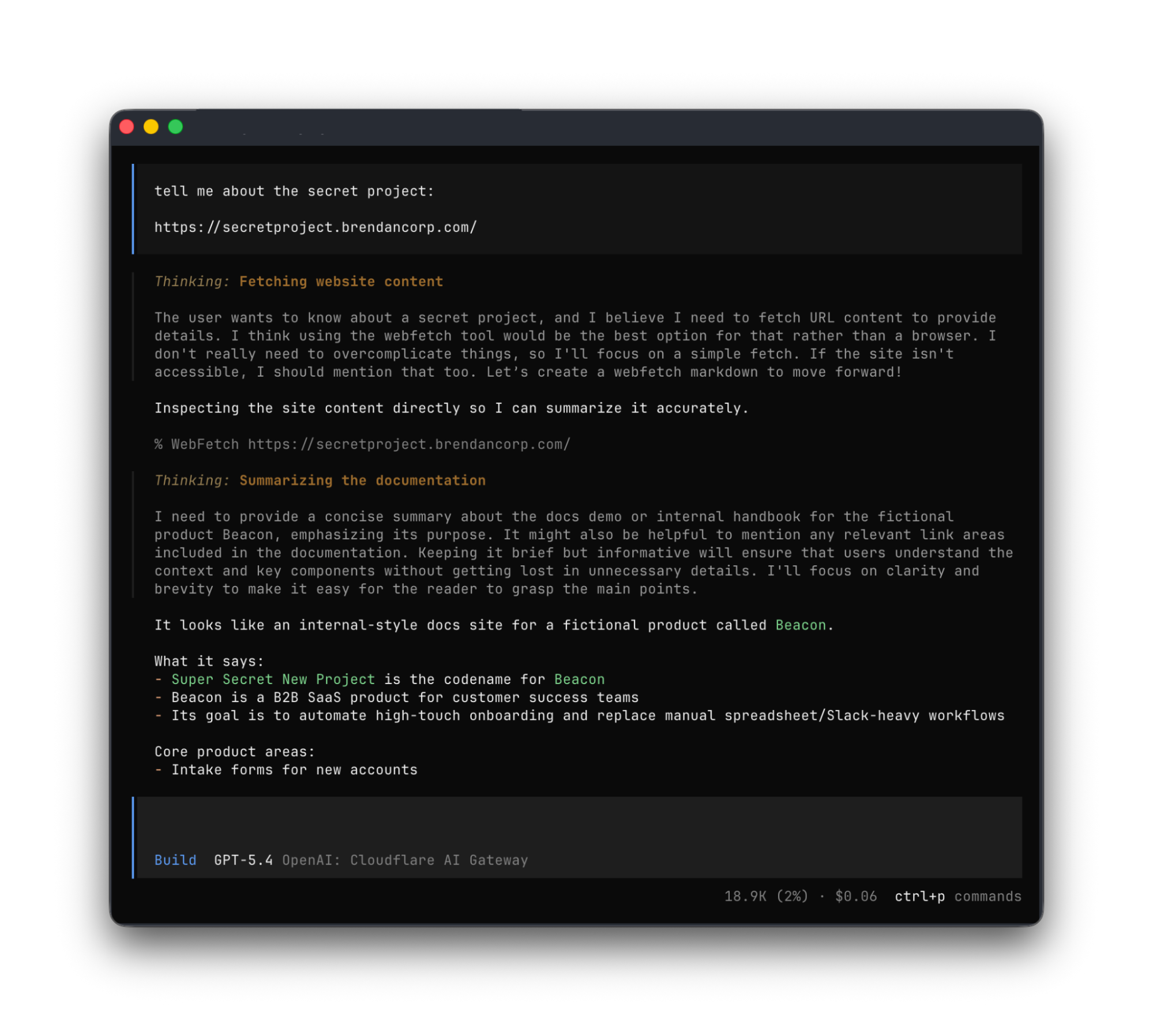
Any agent from Codex to Claude Code to Goose and beyond can implement this, and there’s nothing bespoke to Cloudflare. It’s all built using OAuth standards.
We think this flow is powerful, and that supporting RFC 9728 can help agents with more than just making basic web fetch requests. If a REST API supports RFC 9728 (and the agent does too), the agent has everything it needs to start making authenticated requests against that API. If the REST API supports RFC 9727, then the client can discover a catalog of REST API endpoints on its own, and do even more without additional documentation, agent skills, MCP servers or CLIs.
Each of these play important roles with agents — Cloudflare itself provides an MCP server for the Cloudflare API (built using Code Mode), Wrangler CLI, and Agent Skills, and a Plugin. But supporting RFC 9728 helps ensure that even when none of these are preinstalled, agents have a clear path forward. If the agent has a sandbox to execute untrusted code, it can just write and execute code that calls the API that the human has granted it access to. We’re working on supporting this for Cloudflare’s own APIs, to help your agents understand how to use Cloudflare.
At Cloudflare our own internal apps are deployed to dozens of different Cloudflare accounts, which are all part of an Organization — a newly introduced way for administrators to manage users, configurations, and view analytics across many Cloudflare accounts. We have had the same challenge as many of our customers: each Cloudflare account has to separately configure an IdP, so Cloudflare Access uses our identity provider. It’s critical that this is consistent across an organization — you don’t want one Cloudflare account to inadvertently allow people to sign in just with a one-time PIN, rather than requiring that they authenticate via single-sign on (SSO).
To solve this, we’re currently working on making it possible to share an identity provider across Cloudflare accounts, giving organizations a way to designate a single primary IdP for use across every account in their organization.
As new Cloudflare accounts are created within an organization, administrators will be able to configure a bridge to the primary IdP with a single click, so Access applications across accounts can be protected by one identity provider. This removes the need to manually configure IdPs account by account, which is a process that doesn’t scale for organizations with many teams and individuals each operating their own accounts.
Across companies, people in every role and business function are now using agents to build internal apps, and expect their agents to be able to access context from internal apps. We are responding to this step function growth in internal software development by making the Workers Platform and Cloudflare One work better together — so that it is easier to build and secure internal apps on Cloudflare.
Expect more to come soon, including:
-
More direct integration between Cloudflare Access and Cloudflare Workers, without the need to validate JWTs or remember which of many routes a particular Worker is exposed on.
-
wrangler dev –tunnel — an easy way to expose your local development server to others when you’re building something new, and want to share it with others before deploying
-
A CLI interface for Cloudflare Access and the entire Cloudflare API
-
More announcements to come during Agents Week 2026
Managed OAuth is now available, in open beta, to all Cloudflare customers. Head over to the Cloudflare dashboard to enable it for your Access applications. You can use it for any internal app, whether it’s one built on Cloudflare Workers, or hosted elsewhere. And if you haven’t built internal apps on the Workers Platform yet — it’s the fastest way for your team to go from zero to deployed (and protected) in production.
Secure private networking for everyone: users, nodes, agents, Workers — introducing Cloudflare Mesh
Post Syndicated from Nikita Cano original https://blog.cloudflare.com/mesh/
AI agents have changed how teams think about private network access. Your coding agent needs to query a staging database. Your production agent needs to call an internal API. Your personal AI assistant needs to reach a service running on your home network. The clients are no longer just humans or services. They’re agents, running autonomously, making requests you didn’t explicitly approve, against infrastructure you need to keep secure.
Each of these workflows has the same underlying problem: agents need to reach private resources, but the tools for doing that were built for humans, not autonomous software. VPNs require interactive login. SSH tunnels require manual setup. Exposing services publicly is a security risk. And none of these approaches give you visibility into what the agent is actually doing once it’s connected.
Today, we’re introducing Cloudflare Mesh to connect your private networks together and provide secure access for your agents. We’re also integrating Mesh with Cloudflare Developer Platform so that Workers, Durable Objects, and agents built with the Agents SDK can reach your private infrastructure directly.
If you’re using Cloudflare One’s SASE and Zero Trust suite, you already have access to Mesh. You don’t need a new technology paradigm to secure agentic workloads. You need a SASE that was built for the agentic era, and that’s Cloudflare One. Cloudflare Mesh is a new experience with a simpler setup that leverages the on-ramps you’re already familiar with: WARP Connector (now called a Cloudflare Mesh node) and WARP Client (now called Cloudflare One Client). Together, these create a private network for human, developer, and agent traffic. Mesh is directly integrated into your existing Cloudflare One deployment. Your existing Gateway policies, Access rules, and device posture checks apply to Mesh traffic automatically.
If you’re a developer who just wants private networking for your agents, services, and team, Mesh is where you start. Set it up in minutes, connect your networks, and secure your traffic. And because Mesh runs on the Cloudflare One platform, you can grow into more advanced capabilities over time: Gateway network, DNS, and HTTP policies for fine-grained traffic control, Access for Infrastructure for SSH and RDP session management, Browser Isolation for safe web access, DLP to prevent sensitive data from leaving your network, and CASB for SaaS security. You won’t have to plan for all of this on day one. You just don’t have to migrate when you need it.
Private networking has always been about connecting clients to resources — SSH into a server, query a database, access an internal API. What’s changed is who the clients are. A year ago, the answer was your developers and your services. Today, it’s increasingly your agents.
This isn’t theoretical. Look at the ecosystem: the explosion of MCP (Model Context Protocol) servers providing tool access, coding agents that need to read from private repos and databases, personal assistants running on home hardware. Each of these patterns assumes the agent can reach the resources it needs. When those resources are isolated in private networks, the agent is stuck.
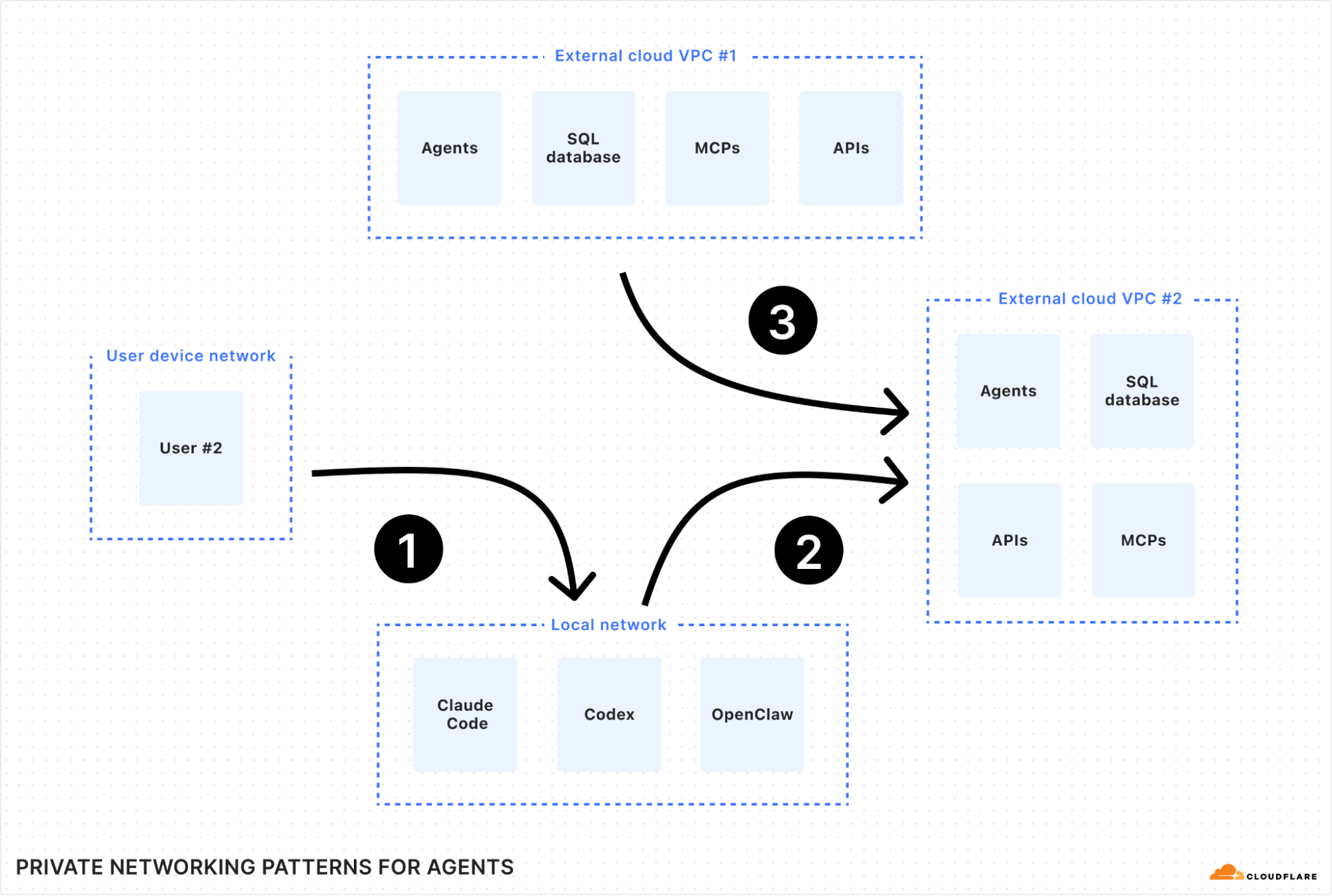
This creates three workflows that are hard to secure today:
-
Accessing a personal agent from a mobile device. You’re running OpenClaw on a Mac mini at home. You want to reach it from your phone, your laptop at a coffee shop, or your work machine. But exposing it to the public Internet (even behind a password) can leave some gaps exposed. Your agent has shell access, file system access, and network access to your home network. One misconfiguration and anyone can reach it.
-
Letting a coding agent access your staging environment. You’re using Claude Code, Cursor, or Codex on your laptop. You ask it to check deployment status, query analytics from a staging database, or read from an internal object store. But those services live in a private cloud VPC, so your agent can’t reach them without exposing them to the Internet or tunneling your entire laptop into the VPC.
-
Connecting deployed agents to private services. You’re building agents into your product using the Agents SDK on Cloudflare Workers. Those agents need to call internal APIs, query databases, and access services that aren’t on the public Internet. They need private access, but with scoped permissions, audit trails, and no credential leakage.
Cloudflare Mesh is developer-friendly private networking. One lightweight connector, one binary, connects everything: your personal devices, your remote servers, your user endpoints. You don’t need to install separate tools for each pattern. One connector on your network, and every access pattern works.
Once connected, devices in your private network can talk to each other over private IPs, routed through Cloudflare’s global network across 330+ cities giving you better reliability and control over your network.
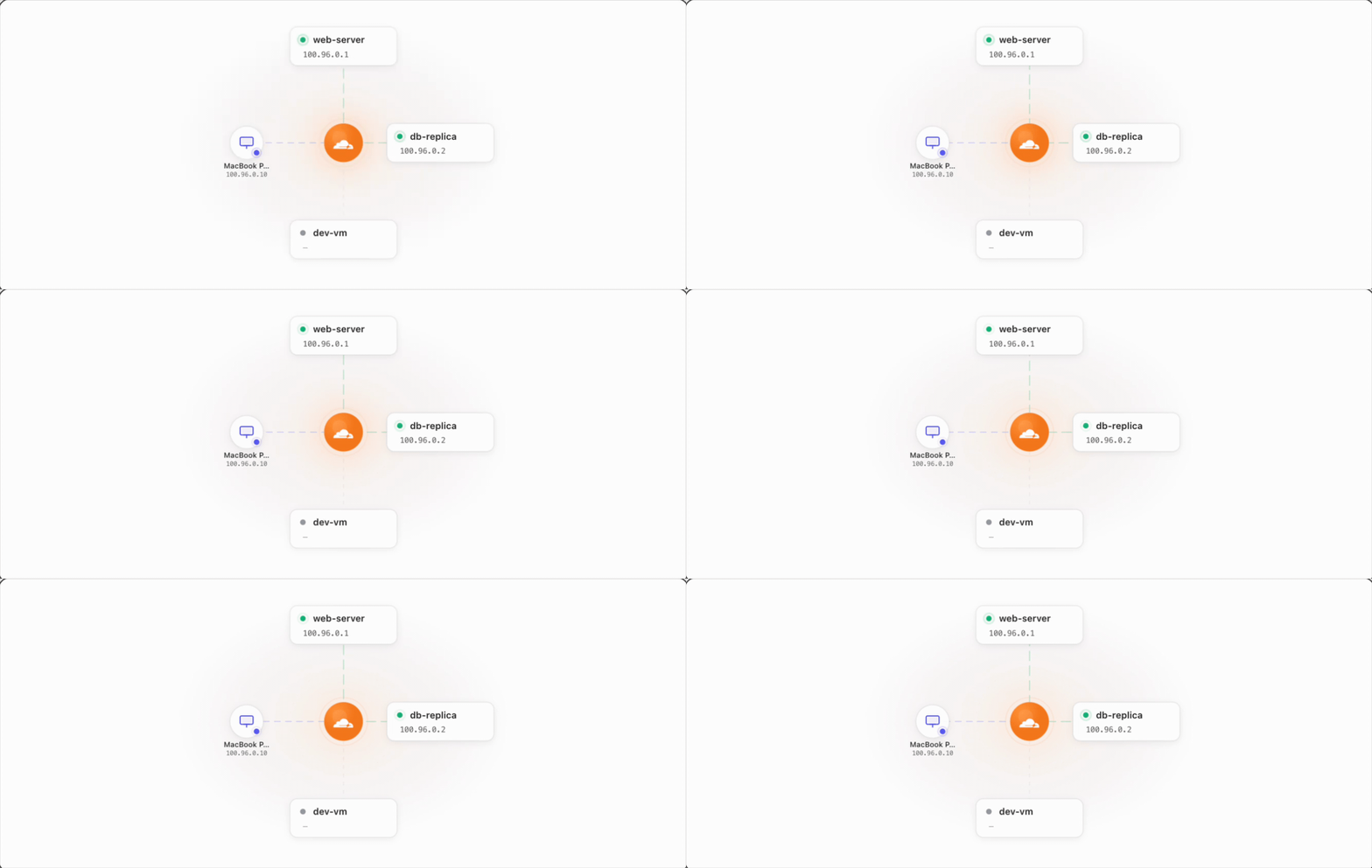
Now, with Mesh, a single solution can solve all of the agent scenarios we mentioned above:
-
With Cloudflare One Client for iOS on your phone, you can securely connect your mobile devices to your local Mac mini running OpenClaw via a Mesh private network.
-
With Cloudflare One Client for macOS on your laptop, you can connect your laptop to your private network so your coding agents can reach staging databases or APIs and query them.
-
With Mesh nodes on your Linux servers, you can connect VPCs in external clouds together, letting agents access resources and MCPs in external private networks.
Because Mesh is powered by Cloudflare One Client, every connection inherits the security controls of the Cloudflare One platform. Gateway policies apply to Mesh traffic. Device posture checks validate connecting devices. DNS filtering catches suspicious lookups. You get this without additional configuration: the same policies that protect your human traffic protect your agent traffic.
With the introduction of Mesh, you might ask: when should I use Mesh instead of Tunnel? Both connect external networks privately to Cloudflare, but they serve different purposes. Cloudflare Tunnel is the ideal solution for unidirectional traffic, where Cloudflare proxies the traffic from the edge to specific private services (like a web server or a database).
Cloudflare Mesh, on the other hand, provides a full bidirectional, many-to-many network. Every device and node on your Mesh can access one another using their private IPs. An application or agent running in your network can discover and access any other resource on the Mesh without each resource needing its own Tunnel.
Cloudflare Mesh gives you the benefits of a mesh network (resiliency, high scalability, low latency and high performance), but, by routing everything through Cloudflare, it resolves a key challenge of mesh networks: NAT traversal.
Most of the Internet is behind NAT (Network Address Translation). This mechanism allows an entire local network of devices to share a single public IP address by mapping traffic between public headers and private internal addresses. When two devices are behind NAT, direct connections can fail and traffic has to fall back to relay servers. If your relay infrastructure has limited points of presence, a meaningful fraction of your traffic hits those relays, adding latency and reducing reliability. And while it can be possible to self-host your own relay servers to compensate, that means taking on the burden of managing additional infrastructure just to connect your existing network.
Cloudflare Mesh takes a different approach. All Mesh traffic routes through Cloudflare’s global network, the same infrastructure that serves traffic for some of the largest websites of the Internet. For cross-region or multi-cloud traffic, this consistently beats public Internet routing. There’s no degraded fallback path, because the Cloudflare edge is the path.
Routing through Cloudflare also means every packet passes through Cloudflare’s security stack. This is the key advantage of building Mesh on the Cloudflare One platform: security isn’t a separate product you bolt on later. And by leveraging this same global backbone, we can provide these core pillars to every team from day one:
50 nodes and 50 users free. Your whole team and your whole staging environment on one private network, included with every Cloudflare account.
Global edge routing. 330+ cities, optimized backbone routing. No relay servers with limited points of presence. No degraded fallback paths.
Security controls from day one. Mesh runs on Cloudflare One. Gateway policies, DNS filtering, DLP, traffic inspection, and device posture checks are all available on the same platform. Start with simple private connectivity. Turn on Gateway policies when you need traffic filtering. Enable Access for Infrastructure when you need session-level controls for SSH and RDP. Add DLP when you need to prevent sensitive data from leaving your network. Every capability is one toggle away.
High availability. Create a Mesh node with high availability enabled and spin up multiple connectors using the same token in active-passive mode. They advertise the same IP routes, so if one goes down, traffic fails over automatically.
Mesh connects your agents and resources across external clouds, but you also need to be able to connect from your agents built on Workers with Agents SDK as well. To enable this, we’ve extended Workers VPC to make your entire Mesh network accessible to Workers and Durable Objects.
That means that you can connect to your Cloudflare Mesh network from Workers, making the entire network accessible from a single binding’s fetch() call. This complements Workers VPC’s existing support for Cloudflare Tunnel, giving you more choice over how you want to secure your networks. Now, you can specify entire networks that you want to connect to in your wrangler.jsonc file. To bind to your Mesh network, use the cf1:network reserved keyword that binds to the Mesh network of your account:
"vpc_networks": [
  { "binding": "MESH", "network_id": "cf1:network", "remote": true },
  { "binding": "AWS_VPC", "tunnel_id": "350fd307-...", "remote": true }
]
Then, you can use it within your Worker or agent code:
export default {
  async fetch(request: Request, env: Env, ctx: ExecutionContext) {
    // Reach any internal host on your Mesh, no pre-registration required
    const apiResponse = await env.MESH.fetch("http://10.0.1.50/api/data");

    // Internal hostname resolved via tunnel's private DNS resolver
    const dbResponse = await env.AWS_VPC.fetch("http://internal-db.corp.local:5432");

    return new Response(await apiResponse.text());
  },
};
By connecting the Developer Platform to your Mesh networks, you can build Workers that have secure access to your private databases, internal APIs and MCPs, allowing you to build cross-cloud agents and MCPs that provide agentic capabilities to your app. But it also opens up a world where agents can autonomously observe your entire stack end-to-end, cross-reference logs and suggest optimizations in real-time.
Together, Cloudflare Mesh, Workers VPC, and the Agents SDK provide a unified private network for your agents that spans both Cloudflare and your external clouds. We’ve merged connectivity and compute so your agents can securely reach the resources they need, wherever they live, across the globe.

Mesh nodes are your servers, VMs, and containers. They run a headless version of Cloudflare One Client and get a Mesh IP. Services talk to services over private IPs, bidirectionally, routed through Cloudflare’s edge.
Devices are your laptops and phones. They run the Cloudflare One Client and reach Mesh nodes directly: SSH, database queries, API calls, all over private IPs. Your local coding agents use this connection to access private resources.
Agents on Workers reach private services through Workers VPC Network bindings. They get scoped access to entire networks, mediated by MCP. The network enforces what the agent can reach. The MCP server enforces what the agent can do.
The current version of Mesh provides the foundation for secure, unified connectivity. But as agentic workflows become more complex, we’re focused on moving beyond simple connectivity toward a network that is more intuitive to manage and more granularly aware of who, or what, is talking to your services. Here is what we are building for the rest of the year.
We’re extending Cloudflare Tunnel’s hostname routing to Mesh this summer. Your Mesh nodes will be able to attract traffic for private hostnames like wiki.local or api.staging.internal, without you having to manage IP lists or worry about how those hostnames resolve on the Cloudflare edge. Route traffic to services by name, not by IP. If your infrastructure uses dynamic IPs, auto-scaling groups, or ephemeral containers, this removes an entire class of routing headaches.
Today, you reach Mesh nodes by their Mesh IPs: ssh 100.64.0.5. That works, but it’s not how you think about your infrastructure. You think in names: postgres-staging, api-prod, nikitas-openclaw.
Later this year we’re building Mesh DNS so that every node and device that joins your Mesh automatically gets a routable internal hostname. No DNS configuration or manual records. Add a node named postgres-staging, and postgres-staging.mesh resolves to the right Mesh IP from any device on your Mesh.
Combined with hostname routing, you’ll be able to ssh postgres-staging.mesh or curl http://api-prod.mesh:3000/health without ever knowing or managing an IP address.
Today, Mesh nodes authenticate to the Cloudflare edge, but they share an identity at the network layer. Devices authenticate with user identity via the Cloudflare One Client, but nodes don’t yet carry distinct, routable identities that Gateway policies can differentiate.
We want to change that. The goal is identity-aware routing for Mesh, where each node, each device, and eventually each agent gets a distinct identity that policies can evaluate. Instead of writing rules based on IP ranges, you write rules based on who or what is connecting.
This matters most for agents. Today, when an agent running on Workers calls a tool through a VPC binding, the target service sees a Worker making a request. It doesn’t know which agent is calling, who authorized it, or what scope was granted. On the Mesh side, when a local coding agent on your laptop reaches a staging service, Gateway sees your device identity but not the agent’s.
We’re working toward a model where agents carry their own identity through the network:
-
Principal / Sponsor: The human who authorized the action (Nikita from the platform team)
-
Agent: The AI system performing it (the deployment assistant, session #abc123)
-
Scope: What the agent is allowed to do (read deployments, trigger rollbacks, nothing else)
This would let you write policies like: reads from Nikita’s agents are allowed, but writes require Nikita directly. Agent traffic can be filtered independently from human traffic. An agent’s network access can be revoked without touching Nikita’s.
The infrastructure for this is in place. Mesh nodes provision with per-node tokens, devices authenticate with per-user identity, and Workers VPC bindings scope per-service access. The missing piece is making these identities visible to the policy layer so Gateway can make routing and access decisions based on them. That’s what we’re building.
Today, Mesh nodes run on VMs and bare-metal Linux servers. But modern infrastructure increasingly runs in containers: Kubernetes pods, Docker Compose stacks, ephemeral CI/CD runners. We’re building a Mesh Docker image that lets you add a Mesh node to any containerized environment.
This means you’ll be able to include a Mesh sidecar in your Docker Compose stack and give every service in that stack private network access. A microservice running in a container in your staging cluster could reach a database in your production VPC over Mesh, without either service needing a public endpoint.
It is also useful for CI/CD pipelines that can access private infrastructure during builds and tests: your GitHub Actions runner pulls the Mesh container image, joins your network, runs integration tests against your staging environment, and tears down. All without VPN credentials to manage or persistent tunnels to maintain: the node disappears when the container exits.
We expect the Mesh Docker image to be available later this year.
While we continue to evolve these identity and routing capabilities, the foundation for secure, unified networking is available today. You can start bridging your clouds and securing your agents in just a few minutes.
Get started Cloudflare Mesh: Head to Networking > Mesh in the Cloudflare dashboard. Free for up to 50 nodes and 50 users.
Build agents with Agents SDK and Workers VPC: Install the Agents SDK (`npm i agents`), follow the Workers VPC quickstart, and build a remote MCP server with private backend access.
Already on Cloudflare One? Mesh works with your existing setup. Your Gateway policies, device posture checks, and access rules apply to Mesh traffic automatically. See the Mesh documentation to add your first node.

Your Cloud Detection Strategy in 2026: What to Expect at the Global Cybersecurity Summit
Post Syndicated from Emma Burdett original https://www.rapid7.com/blog/post/it-2026-cloud-detection-strategy-global-cybersecurity-summit
Cloud environments have changed how security teams detect and respond to threats. Signals come from more places, identities are harder to track, and attacks rarely stay within a single system. For many teams, the challenge is no longer visibility. It is having the risk context to understand what matters and act on it quickly. This shift is reflected in the conversations shaping this year’s Rapid7 Global Cybersecurity Summit.
Taking place May 12-13, the summit explores how detection and response are evolving across cloud, identity, and endpoint environments. The focus is practical: how attacks actually unfold, how teams respond under pressure, and how detection strategies need to adapt.
Detection is no longer just about coverage
One of the clearest themes across the agenda is that traditional detection models are struggling to keep pace with attackers. Environments are more dynamic, and attackers are more targeted. Catching everything is no longer realistic, and in many cases it is not useful.
Sessions like The New Rules of Detection Engineering will examine this shift in detail. The focus moves away from volume and toward precision. It will ask questions like: What makes a detection meaningful? How should teams prioritize signals? And how can detection strategies support real outcomes rather than just generate alerts? This is especially important in cloud environments, where context changes quickly and signals are often incomplete.
Understanding how attacks actually unfold
To improve detection, teams need to understand how attacks behave in practice. Several sessions across the summit focus on this directly.
The Reality of Running a SOC in 2026 will explore how modern attacks begin — from identity misuse to cloud misconfigurations— and how they evolve over time. Rather than following a predictable path, attacks move across systems, taking advantage of gaps in visibility and delayed decisions.
This theme continues in sessions like Inside the Modern SOC, where attendees follow a real investigation from first alert to outcome. These walkthroughs show how signals are correlated across environments and how decisions are made when time and clarity are limited.
From exposure to runtime risk
Cloud security also requires a closer connection between exposure and detection. In many cases, incidents begin long before an alert is triggered.
Sessions such as From Cloud Exposure to Runtime Attack explore how misconfigurations, permissions, and overlooked risks lead to active threats. The focus is on how teams connect exposure insights with runtime behavior to improve prioritization and respond earlier in the attack lifecycle.
This is a practical shift. Detection is no longer a separate function but part of a broader process that starts with understanding exposure and continues through to response.
What this means for security teams
Across these sessions, a consistent message emerges: Detection strategies need to be grounded in how environments actually behave, not how they are expected to behave.
This means focusing on signal quality rather than volume, connecting data across cloud, identity, and endpoint, and building workflows that support faster decisions. It also means accepting that not all alerts have equal weight, and that prioritization is a core part of modern detection.
A preview of what’s to come
Cloud detection is just one part of a broader shift happening across the summit. Sessions on MDR, AI, and exposure management all connect back to the same idea. Security operations must move earlier, reduce noise, and act with greater confidence.
If you are rethinking how your team detects and responds to threats in cloud and hybrid environments, this is where those conversations come together.
Join us May 12–13 and see how security teams are evolving their detection strategies for 2026.
How Hackers Are Thinking About AI
Post Syndicated from Bruce Schneier original https://www.schneier.com/blog/archives/2026/04/how-hackers-are-thinking-about-ai.html
Interesting paper: “What hackers talk about when they talk about AI: Early-stage diffusion of a cybercrime innovation.”
Abstract: The rapid expansion of artificial intelligence (AI) is raising concerns about its potential to transform cybercrime. Beyond empowering novice offenders, AI stands to intensify the scale and sophistication of attacks by seasoned cybercriminals. This paper examines the evolving relationship between cybercriminals and AI using a unique dataset from a cyber threat intelligence platform. Analyzing more than 160 cybercrime forum conversations collected over seven months, our research reveals how cybercriminals understand AI and discuss how they can exploit its capabilities. Their exchanges reflect growing curiosity about AI’s criminal applications through legal tools and dedicated criminal tools, but also doubts and anxieties about AI’s effectiveness and its effects on their business models and operational security. The study documents attempts to misuse legitimate AI tools and develop bespoke models tailored for illicit purposes. Combining the diffusion of innovation framework with thematic analysis, the paper provides an in-depth view of emerging AI-enabled cybercrime and offers practical insights for law enforcement and policymakers.
What Donald Trump’s Social-Media Posts Say About His Views on Religion
Post Syndicated from The Atlantic original https://www.youtube.com/shorts/jZV8xMHPk6g
Comparing compression tools
Post Syndicated from arp242.net original https://www.arp242.net/cmp-compress.html
I’d like to know what the “best” compression tool is for storing archives
(backups, data files). So I wrote a tool to compare them: cmp-compress.
My tl;dr take-away is:
zstd -3for fast compression (the default).xz -7for the best ratio use;-8or-9sometimes compress better but
often don’t. You probably want to test this.zstd -12for a good trade-off that leans towards fast.zstd -17for a good trade-off that leans towards better ratio.- Add
-T0to zstd to use all cores if nothing else is running on the system
(or use thezstdmtwrapper).
For other use-cases all of this may of course be different.
Some tools like xz and zstd offer many differs knobs and levers; I’m sure these
are useful but did not bother with them and tested only the presets. I’m not
looking for an incantation to eek out the absolute best – I just want an
informed practical decision on which tool to use with which flags to compress
common stuff.
For the same reason I’m only comparing reasonably common compression tools
already in wide-spread use. There are many others that are very similar to those
listed here with minor differences (e.g. zip, 7zip), not considered stable (e.g.
bzip3), or just not widespread for one reason or the other.
If you’re interested in other tools or sets of flags then you can run
cmp-compress yourself.
Full Results as HTML table: /compress.html.
Or as JSON: /compress.json.
I ran this on the following files:
| vim | 5.5M | Statically linked binary |
| qemu-system-x86_64 | 29M | Dynamically linked binary |
| dockerd | 87M | Statically linked binary |
| dickens | 9.7M | English text, no tags |
| enwik8 | 95M | English text, with XML and Wiki tags |
| enwik9 | 950M | English text, with XML and Wiki tags |
| yt-dlp-2026.03.17.tar | 12M | Python code |
| coreutils-9.10.tar | 63M | C code |
| go1.26.1.src.tar | 150M | Go code |
| go1.26.1.linux-amd64.tar | 233M | Mix of Go code and statically linked binaries |
The enwik files are from the Large Text Compression Benchmark; dickens is from
the Silesia compression corpus; QEMU is version 10.2.0; Docker is version
29.4.0, and vim is a private modified fork that’s not easy to exactly reproduce
but a statically linked huge build of Vim 9.1 should be close.
All of this is run on Void Linux with Linux 6.19.10 on a ThinkPad x13 with AMD
Ryzen 7 7840U (8 cores/16 threads) and 32G of memory. I ran all the tests twice
and discarded the first run (cmp-compress compare >/dev/null && cmp-compress compare >a.json).
gzip
The -# flag has a small effect and becomes useless above -6. Even the difference
between -5 and -6 is quite small, and arguably -5 would be a better default than
-6. -4 is a good setting if you want to be faster as it compresses a bit more
than -1, -2, and -3, but isn’t too much slower.
The -# flag makes no meaningful difference for decompression times.
In short, use only -4, -5, or -6.
pigz
The -# behaves identical to gzip: it has no meaningful difference from gzip
(in most cases pigz compresses slightly better – by a negligible amount but
still). It’s often faster when using multiple threads, but single-thread
compression is a bit slower.
It also adds a -11 flag to use the zopfli algorithm. The manpage says it “gives
a few percent better compression at a severe cost in execution time”. It’s not
exaggerating about the “severe cost”: it’s always the slowest of any tool by a
huge margin. I suppose that it can be useful if you’re serving things at
Google-scale, but you’re probably not, and other algorithms (brotli, zstd) are
now widely-implemented. I’m going to say that in 2026 it’s useless: bzip2, xz,
and zstd can all achieve better compression while being much much faster.
Aside: I kind of wish /bin/gzip would be replaced by pigz, or that gzip would
use zlib and incorporate multi-threaded code. pigz seems stable, reasonably
coded, and generally fairly good. I can’t find any reasons to not s/gzip/pigz/
other than vague concerns about “it’s different”, which is not entirely invalid
but pigz has been around for a long time and at some point things need to move
forward.
bzip2
The classic “I’m okay waiting a bit longer than gzip to get better ratios”. As a
rule, compression is ~1.5 times slower, and decompression is ~3 times slower. It
practically always gets a better compression ratio than gzip. More so on text
than on binary files.
The -# flags make a small difference in compression ratio or time. There is no
reason to use anything other than -9 (the default). bzip3 did away with -#
flags entirely.
Both xz and zstd compress better than bzip2, but do take longer. Only on the
dickens file does bzip2 give the same compression ratio as xz, but bzip2 is an
order of a magnitude faster. Overall I’m going to say that bzip2 is rarely worth
it, except perhaps if your data is primary text with minimal formatting (e.g.
Markdown files, or similar). I don’t know to what degree this holds true for
other languages or scripts as I only tested English.
xz
The newer “I’m okay waiting a bit longer than gzip to get better ratios”. Both
compression and decompression is fairly slow, but delivers the best ratios of
the common compression tools (zstd comes close, but xz is still meaningfully
better).
The -# flag does little above -5, albeit more than gzip and there is a small but
meaningful difference between the levels. For many files -8 and -9 are much
slower than -7 while having little to no effect on ratio. As a rule you want to
stick with the default of -6 unless you’ve tested it makes a meaningful
difference on your data.
On binary files it outperforms bzip2 even on -0, on code at around -1, and on
natural language it tends to outperform bzip2 at around -4 or -5,
Decompression speed decreases with higher -# flags, although this is not quite
linear and sometimes higher -# flags have faster decompression speeds.
Sometimes it’s very slow (e.g. enwik9 is almost two minutes to decompress,
which is by far the slowest other than pigz -11.
zstd
Unlike gzip and xz the -# flag makes a meaningful difference at any level. The
progression from -1 to -19 isn’t linear, but comes closer than anything else. In
particular, the gap between -12 to -13 is consistently large with -13 being two
to three times slower than -12.
Decompression is fast, although does take a noticeable hit at higher -# levels,
but even at -19 it’s always faster than xz -0.
It’s almost always faster than gzip -1 at lower -# levels while delivering a
better compression ratio. -12 is usually faster than gzip -6 (and -13 is slower,
due to aforementioned jump).
For natural language files it compresses better than bzip2 at around -16, while
being much slower. For code and binary files it’s around -6, while being faster.
xz still compresses ~10% better than zstd -19, but xz is slower (often a lot
slower).
The –ultra flags eeks out a slightly amount of extra compression ratio at the
expense of being a lot slower, although not quite as dramatic as pigz -11. The
compression ratio differences are small enough that for most cases it’s rarely
useful.
–fast is not that much faster than -1 and compression ratio suffers greatly,
and decompression performance is not significantly faster. There’s probably
some uses cases where you really want to get the maximum compression
performance, but by and large, I’m going to say it’s not very useful for most
cases, outside of some streaming perhaps.
Conclusion
I’m going to say that “just use zstd” is probably decent advice: it doesn’t have
the absolute best compression ratio or performance, but for many use-cases the
trade-of it makes are quite good, and it has very fast decompression which is
nice. zstd also has a bewildering number of configuration options, making it
very flexible: e.g. for smaller files the ability to pre-train a dictionary will
make a big difference (not tested in this overview: based on previous
experience).
If you do need absolute maximum compression ratios then xz is often better, at
the expense of being much slower. In some cases that’s a good trade-off.
For natural language text bzip2 might still be worth it, but compression seems
to suffer if there’s too much formatting (which is often the case in real-world
files). bzip3 seems an interesting improvement over bzip2, but the big bold
“decompression may not work” disclaimer is rather a turn-off at the moment. I
suppose one could use a wrapper which compares the decompression results with
the input. That said, out of the tools not included here, bzip3 seems the most
interesting. Also see: An ode to bzip.
I want to stress once more that all of this may depend on your specific data,
system you’re using, planetary alignments, etc. “Most of the time”, “often”, and
“usually” do not equal “always”.
Hungarians Cheer Orbán’s Loss
Post Syndicated from The Atlantic original https://www.youtube.com/shorts/WxmT7HY-ris
Acemagic M1A PRO+ Review An AMD-Powered 128GB AI Mini PC
Post Syndicated from Ryan Smith original https://www.servethehome.com/acemagic-m1a-pro-review-an-amd-powered-128gb-ai-mini-pc/
We test the Acemagic M1A Pro+ a neat looking AI-focused mini PC with the AMD Ryzen AI Max+ 395 and 128GB of LPDDR5X memory
The post Acemagic M1A PRO+ Review An AMD-Powered 128GB AI Mini PC appeared first on ServeTheHome.
Избори 2026-та – обновени секции в чужбина, съвети за процеса на гласуване
Post Syndicated from Боян Юруков original https://yurukov.net/blog/2026/iz2026-sekcii-final/
На 19-ти април ще се проведат избори за Народно събрание. Остават само няколко дни и имаме на разположение по-малко секции в чужбини, в които да упражним правото си на глас, в сравнение с предишни избори. Сред 443-те места, където все пак ще има секции, около 1 от 5 имат променен адрес. Затова съветвам да сверите на картата дали при вашата ще има промени този път. Когато отворите избраната от Вас през линка, бихте могли да споделите в социалните мрежи, че ще гласувате там призовавайки и другите да го сторят.
Ето няколко важни неща, които трябва да знаете:
- Изборният ден започва в 7:00 сутринта местно време и свършва в 8:00 часа вечерта
- Може да гласува всеки български гражданин независимо дали е подал заявление или не. Тогава просто попълвате на място декларация по приложение 28, за да ви добавят в списъка.
- Гласува се с валидна българска лична карта или паспорт.
- Секциите отбелязани горе са актуални към 10-ти април. Възможно е в следващата седмица да има промени или корекции. Затова Ви препоръчвам да проверите преди изборния ден отново на картата и на сайта на МВнР.
- Независимо от отбелязаната в заявлението Ви секция, ако сте подали въобще такова, може да гласувате където и да е в чужбина.
- Извън България може да гласува всеки български гражданин независимо от обичайното му пребиваване. Това означава, че ако пътувате зад граница по работа или на почивка, може да упражните гласа си в близка до Вас секция. Отново, няма значение дали сте подавали заявление.
- Ако все пак сте в България по време на изборите, може да гласувате само по постоянен адрес. Тогава попълвате приложение 22, че не сте гласували в чужбина и са длъжни да Ви отбележат. Присъствате в списъка и след името Ви е отбелязано МВнР.
- В чужбина за Народно събрание има възможност да гласувате само за партия/коалиция. Възможност за преференции, каквито има в страната, отново няма да има след промени в Изборния кодекс в последния момент, за които писах преди. Запознайте се също с бюлетината.
- Препоръчвам да се гласува с машина, където това е възможно. На картата ще видите тази информация избирайки секция до вас. Гласуването с машина е по-бързо и гарантира, че гласът Ви ще бъде преброен и няма шанс да бъде отбелязан като невалиден.
- Препоръчвам да се гласува възможно най-рано, тъй като опитът показва, че с хартиено гласуване с напредването на деня стават струпвания на някои места. Ако имате съмнения и спомени за такива и имате друга близка секция с по-малко натоварване, препоръчваме да отидете там. На картата на Glasuvam.org може също да споделяте и преглеждате обратна връзка от други колко са чакали на това място.
Мейл с най-близките три секции изпратих на над 3100 абонирани за бюлетина на Glasuvam.org. Ако има промяна по някоя от секциите
Повече информация ще намерите на сайта на ЦИК и МВнР. Тази година ЦИК са добавили секция с често задавани въпроси. МВнР са направили своя карта със секциите, която може да заредите в Google Maps на телефона си, ако ви е по-удобно. Забелязах, че някои промени по адресите на секции не са въведени там 4 дни по-късно та съветвам да сверявате все пак с други източници. Такъв е случая с Нант, Франция и една от секциите в Бурса, Турция.

Тази година виждам, че и Facebook отново напомня за изборите на всички българи в страната и чужбина макар и само с линк към страницата на ЦИК.
Секциите с машинен вот
Заради намаления брой секции и утежнената ситуация с възможността на сънародниците ни зад граница да гласуват, реших да направя отделна карта визуализираща къде има секции с машинен вот. Аналогично преди две седмици направих карта с местата, където е имало секции преди, но сега няма да има заради новия Изборен кодекс.
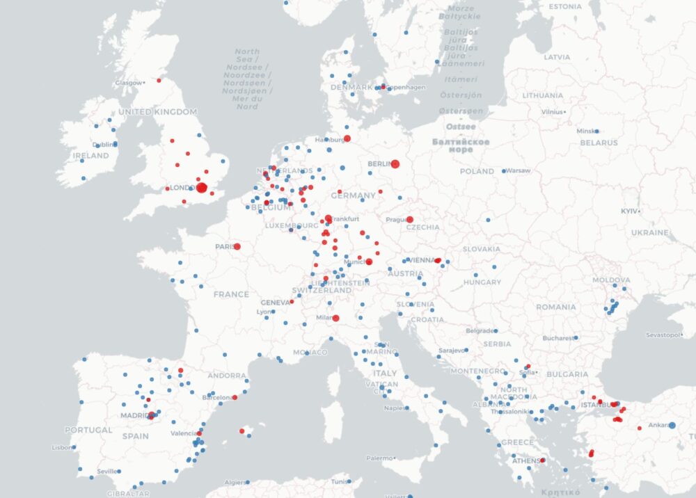
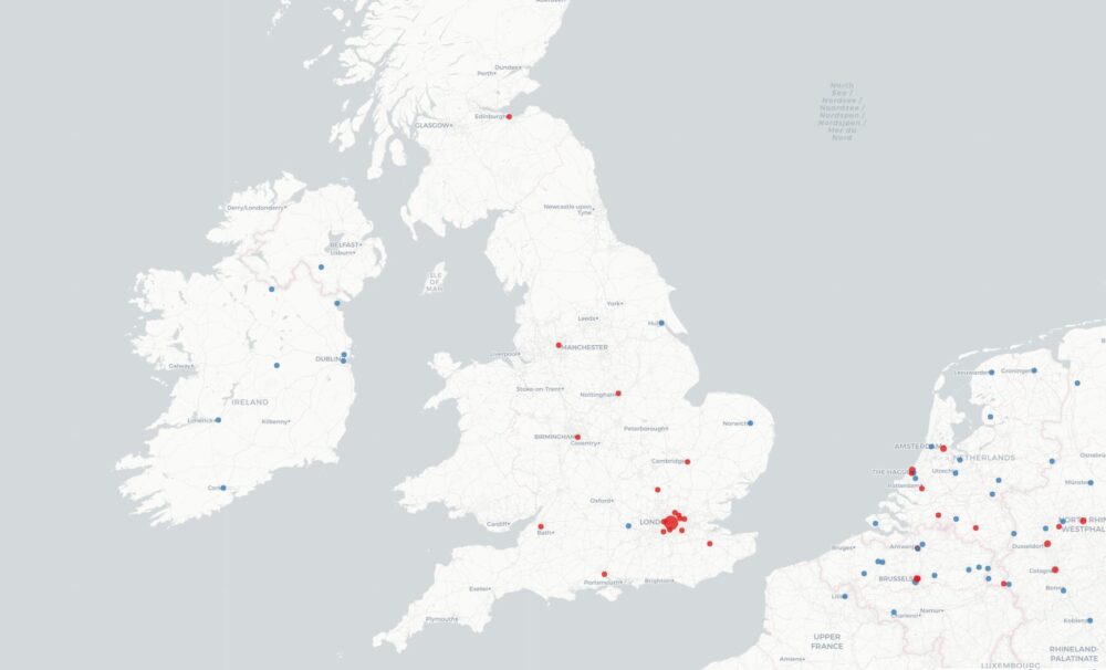
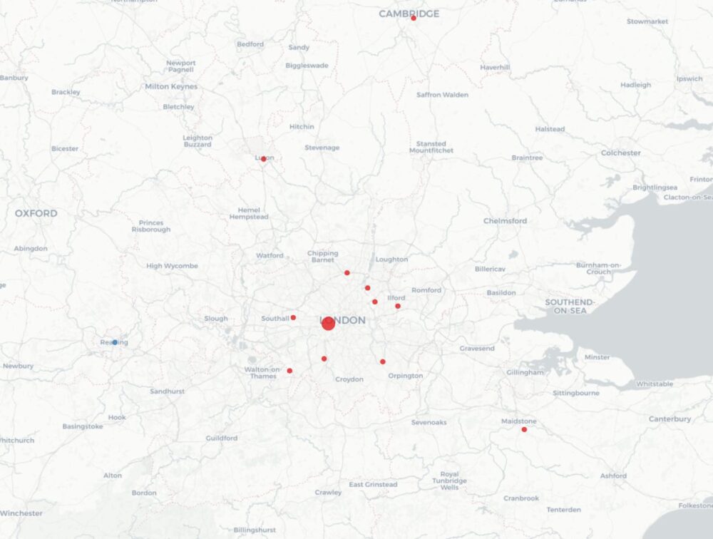
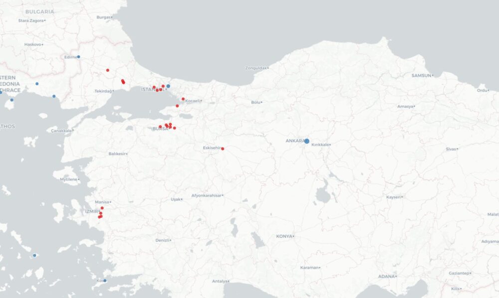
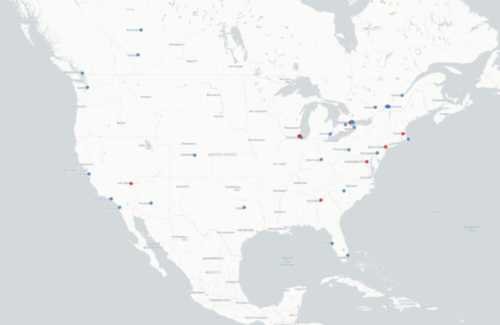
Както споменах по-горе, гласуването с машини не само е по-сигурно и спира редица изборни измами, но е и по-бързо. Вероятно затова ЦИК са решили да концентрират най-много машини във Великобритания и Турция, където натоварването е най-голямо. Тук ще намерите всички секции. В червено са тези, където има поне една секция с машинен вот. Размерът на точките показва колко секции има на това място. Същата информация ще намерите и като избирате отделни места за гласуване в картата със секциите.
Troubleshooting environment with AI analysis in AWS Elastic Beanstalk
Post Syndicated from Chandu Utlapalli original https://aws.amazon.com/blogs/devops/troubleshooting-environment-with-ai-analysis-in-aws-elastic-beanstalk/
Introduction
AWS Elastic Beanstalk simplifies the process of deploying and scaling web applications. You upload your code, and Elastic Beanstalk handles capacity provisioning, load balancing, auto scaling, and application health monitoring.
Elastic Beanstalk now offers AI Analysis to help troubleshoot environment health issues. When you request an analysis, Elastic Beanstalk triggers a script on the Amazon EC2 instance in your environment. The script collects environment events, health data, and instance logs, sends them to Amazon Bedrock for analysis, and uploads the results to Amazon S3. The result is a set of step-by-step troubleshooting recommendations tailored to your environment’s specific issues, helping you reduce mean time to resolution (MTTR).
In the Elastic Beanstalk console, the AI Analysis button appears on the environment overview page when your environment’s health status changes to Warning, Degraded, or Severe. AI analysis is also accessible from the logs page in the console, the AWS CLI, or the EB CLI.
Prerequisites
Before getting started, ensure that you have the following:
- An AWS account with access to AWS Elastic Beanstalk and Amazon Bedrock.
- A supported Elastic Beanstalk platform version – AI analysis is available on Amazon Linux 2 and AL2023 based platform versions released on or after February 16, 2026. Update your environment to a supported platform version if needed.
- Instance profile with required permissions – The managed policies AWSElasticBeanstalkWebTier, AWSElasticBeanstalkWorkerTier, and AWSElasticBeanstalkMulticontainerDocker now include the necessary permissions for AI analysis. Attach one or more of these managed policies to your environment’s instance profile based on your environment tier. If you use a custom instance profile, ensure it includes the following permissions:
bedrock:InvokeModelbedrock:ListFoundationModelselasticbeanstalk:DescribeEventselasticbeanstalk:DescribeEnvironmentHealth
- AWS CLI installed and configured with appropriate permissions. See Installing the AWS CLI.
- Anthropic use case details – AI analysis uses Anthropic Claude models through Amazon Bedrock. Anthropic requires you to submit a one-time use case details form before you can invoke their models. To submit this form, select an Anthropic model from the model catalog in the Amazon Bedrock console, or call the PutUseCaseForModelAccess API. You only need to do this once per AWS account. If you submit the form from the AWS Organizations management account, it automatically covers member accounts in the organization. For more information, see Access Amazon Bedrock foundation models.
- GovCloud Regions – If you are using AWS GovCloud (US) Regions, you must enable access to the latest Anthropic Claude Sonnet and/or Opus model in Amazon Bedrock before using AI analysis. For instructions on enabling model access in GovCloud Regions, see Manage access to Amazon Bedrock foundation models. For information about the latest available Anthropic Claude Sonnet and/or Opus model, see Supported Regions and models for inference profiles.
Solution Overview
In the following sections, we demonstrate how to use AI Analysis to diagnose a Node.js application that fails after a deployment.
- Create a working environment: Deploy a Node.js application to Elastic Beanstalk using the code snippets provided below.
- Break the environment: Update the application with code that requires missing environment variables. This causes the environment health status to transition to Degraded.
- Use AI Analysis: Request an AI Analysis from the Elastic Beanstalk console or the AWS CLI to identify the root cause of the health degradation.
- Apply the fix and verify: Apply the recommendations generated by AI Analysis and confirm that the environment health returns to Ok.
The following figure shows how AI Analysis works:
Figure 1 – AI Analysis architecture
- You initiate a request through the Elastic Beanstalk console (AI Analysis button) or the AWS CLI (RequestEnvironmentInfo API with InfoType set to “analyze”).
- Elastic Beanstalk collects environment data, analyzes it using Amazon Bedrock (a fully managed service that provides access to foundation models through API), and stores the results in Amazon S3.
- You retrieve the results through the console or the RetrieveEnvironmentInfo API using CLI.
Walkthrough
Follow the steps below to set up the sample application, break it, troubleshoot with AI Analysis, and restore the environment to a healthy state.
To try this feature, open your terminal and follow the steps below to create a sample Elastic Beanstalk environment. First, set the following variables. Replace the values with your own unique S3 bucket name and the latest Node.js solution stack for your region. To find the latest solution stack, run aws elasticbeanstalk list-available-solution-stacks.
S3_BUCKET="your-unique-bucket-name"

SOLUTION_STACK_NAME="64bit Amazon Linux 2023 v6.9.0 running Node.js 22"
Setting up the application
We use two versions of a simple Node.js application. The first version (v1-working) is a basic HTTP server that responds to requests successfully. The second version (v2-broken) introduces a dependency on environment variables that are not configured in the Elastic Beanstalk environment, simulating a common deployment issue.
Create a project directory:
mkdir test-app && cd test-app
Create the working application file (v1-working):
cat << 'EOF' > workingapp.js
const http = require('http');

const server = http.createServer((req, res) => {
    res.writeHead(200, { 'Content-Type': 'application/json' });
    res.end(JSON.stringify({ status: 'healthy', message: 'App is running' }));
});

const port = process.env.PORT || 8080;
server.listen(port, () => {
    console.log(`Server running on port ${port}`);
});
EOF
Create the broken application file (v2-broken):
cat << 'EOF' > brokenapp.js
const http = require('http');

// Application requires these environment variables to function
const VAR_1 = process.env.TEST_VARIABLE_1;
const VAR_2 = process.env.TEST_VARIABLE_2;
const VAR_3 = process.env.TEST_VARIABLE_3;

if (!VAR_1 || !VAR_2 || !VAR_3) {
    throw new Error(
        `Missing required environment variables. ` +
        `TEST_VARIABLE_1: ${VAR_1 ? 'set' : 'MISSING'}, ` +
        `TEST_VARIABLE_2: ${VAR_2 ? 'set' : 'MISSING'}, ` +
        `TEST_VARIABLE_3: ${VAR_3 ? 'set' : 'MISSING'}`
    );
}

const server = http.createServer((req, res) => {
    res.writeHead(200, { 'Content-Type': 'application/json' });
    res.end(JSON.stringify({ status: 'healthy', db: VAR_1 }));
});

const port = process.env.PORT || 8080;
server.listen(port, () => {
    console.log(`Server running on port ${port}`);
});
EOF
Create the package.json:
cat << 'EOF' > package.json
{
  "name": "test-app",
  "version": "1.0.0",
  "description": "Sample app that requires environment variables",
  "main": "app.js",
  "scripts": {
    "start": "node app.js"
  }
}
EOF
Create the working application source bundle:
cp workingapp.js app.js

zip -r nodejs-working-app.zip app.js package.json
Create the broken application source bundle:
cp brokenapp.js app.js

zip -r nodejs-broken-app.zip app.js package.json
Step 1: Create a working environment
First, create the Elastic Beanstalk application and deploy the working version.
Create an S3 bucket:
aws s3 mb s3://$S3_BUCKET --region us-east-1
Upload the working application source bundle:
aws s3 cp nodejs-working-app.zip s3://$S3_BUCKET/nodejs-working-app.zip
Create the Elastic Beanstalk application:
aws elasticbeanstalk create-application \
    --application-name test-app \
    --description "Test application" \
    --region us-east-1
Create the application version:
aws elasticbeanstalk create-application-version \
    --application-name test-app \
    --version-label v1-working \
    --source-bundle S3Bucket="$S3_BUCKET",S3Key="nodejs-working-app.zip" \
    --region us-east-1
Create the environment with the working version:
aws elasticbeanstalk create-environment \
    --application-name test-app \
    --environment-name test-app-env \
    --solution-stack-name "$SOLUTION_STACK_NAME" \
    --version-label v1-working \
    --option-settings \
        Namespace=aws:elasticbeanstalk:environment,OptionName=EnvironmentType,Value=SingleInstance \
        Namespace=aws:autoscaling:launchconfiguration,OptionName=IamInstanceProfile,Value=aws-elasticbeanstalk-ec2-role \
    --region us-east-1
Once your environment is created, verify the health:
aws elasticbeanstalk describe-environment-health \
    --environment-name test-app-env \
    --attribute-names All \
    --region us-east-1
Output:
{
    "EnvironmentName": "test-app-env",
    "HealthStatus": "Ok",
    "Status": "Ready",
    "Color": "Green",
    "Causes": [
        "Initialization completed 31 seconds ago and took 2 minutes."
    ],
    "ApplicationMetrics": {
        "RequestCount": 0
    },
    "InstancesHealth": {
        "NoData": 0,
        "Unknown": 0,
        "Pending": 0,
        "Ok": 1,
        "Info": 0,
        "Warning": 0,
        "Degraded": 0,
        "Severe": 0
    },
    "RefreshedAt": "2026-03-25T16:39:11Z"
}

Figure 2 – Environment health showing Ok (Green) status after initial deployment
Step 2: Break the environment
Now, deploy the broken version that requires missing environment variables.
Upload the broken version:
aws s3 cp nodejs-broken-app.zip s3://$S3_BUCKET/nodejs-broken-app.zip
Create the broken application version:
aws elasticbeanstalk create-application-version \
    --application-name test-app \
    --version-label v2-broken \
    --source-bundle S3Bucket="$S3_BUCKET",S3Key="nodejs-broken-app.zip" \
    --region us-east-1
Deploy the broken version:
aws elasticbeanstalk update-environment \
    --environment-name test-app-env \
    --version-label v2-broken \
    --region us-east-1
Within seconds of the deployment completing, the environment health transitions from Ok to Degraded:
aws elasticbeanstalk describe-environment-health \
    --environment-name test-app-env \
    --attribute-names All \
    --region us-east-1
Output:
{
    "EnvironmentName": "test-app-env",
    "HealthStatus": "Degraded",
    "Status": "Ready",
    "Color": "Red",
    "Causes": [
        "Impaired services on all instances."
    ],
    "ApplicationMetrics": {
        "RequestCount": 0
    },
    "InstancesHealth": {
        "NoData": 0,
        "Unknown": 0,
        "Pending": 0,
        "Ok": 0,
        "Info": 0,
        "Warning": 0,
        "Degraded": 0,
        "Severe": 1
    },
    "RefreshedAt": "2026-03-25T16:43:19Z"
}

Figure 3 – Environment health showing Degraded (Red) status with the AI Analysis button visible
Step 3: Use AI Analysis
Request AI analysis from the AWS CLI or the Elastic Beanstalk console. Both methods produce the same results. The CLI approach is useful for automation and scripting, while the console provides a visual workflow where you can view results directly on the environment page. We’ll cover both options below.
Using the AWS CLI
Request the analysis:
aws elasticbeanstalk request-environment-info \
    --environment-name test-app-env \
    --info-type analyze \
    --region us-east-1
Once the request environment operation is completed, retrieve the results:
aws elasticbeanstalk retrieve-environment-info \
    --environment-name test-app-env \
    --info-type analyze \
    --region us-east-1
The response includes an EnvironmentInfo array with a Message field containing a pre-signed S3 URL to the analysis results:
{
    "EnvironmentInfo": [
        {
            "InfoType": "analyze",
            "Ec2InstanceId": "i-1234567890abcdef0",
            "SampleTimestamp": "2026-03-20T20:49:22.763Z",
            "Message": "https://elasticbeanstalk-us-east-1-123456789012.s3.us-east-1.amazonaws.com/resources/environments/logs/analyze/..."
        }
    ]
}
Download and view the analysis:
ANALYSIS_URL=$(aws elasticbeanstalk retrieve-environment-info \
    --environment-name test-app-env \
    --info-type analyze \
    --region us-east-1 \
    --query 'sort_by(EnvironmentInfo, &SampleTimestamp)[-1].Message' \
    --output text)

curl -s "$ANALYSIS_URL"
Figure 4 – AI analysis output retrieved via AWS CLI
Using the Elastic Beanstalk console
When your environment’s health status is Warning, Degraded, or Severe, the AI Analysis button appears in the environment overview section of the Elastic Beanstalk console.
- Navigate to the Elastic Beanstalk console.
- Select your environment (test-app-env).
- On the environment overview page, locate the AI Analysis button that appears when the health status indicates an issue.
- Choose AI Analysis to initiate the analysis.
Video 1 – Requesting AI analysis from the Elastic Beanstalk console
If you want to restart the analysis workflow, you can click on the Reanalyze button to start a new analysis.
Step 4: Apply the fix and verify
The AI analysis identified that the application crashes because the environment does not have three required environment variables configured: TEST_VARIABLE_1, TEST_VARIABLE_2, and TEST_VARIABLE_3. As recommended by the AI analysis, set these environment variables to resolve the issue:
aws elasticbeanstalk update-environment \
    --environment-name test-app-env \
    --option-settings \
        Namespace=aws:elasticbeanstalk:application:environment,OptionName=TEST_VARIABLE_1,Value=value1 \
        Namespace=aws:elasticbeanstalk:application:environment,OptionName=TEST_VARIABLE_2,Value=value2 \
        Namespace=aws:elasticbeanstalk:application:environment,OptionName=TEST_VARIABLE_3,Value=value3 \
    --region us-east-1
After the environment update completes, the application starts successfully and the environment health returns to Ok:
aws elasticbeanstalk describe-environment-health \
    --environment-name test-app-env \
    --attribute-names All \
    --region us-east-1
Output:
{
    "EnvironmentName": "test-app-env",
    "HealthStatus": "Ok",
    "Status": "Ready",
    "Color": "Green",
    "Causes": [
        "Configuration update completed 72 seconds ago and took 54 seconds."
    ],
    "ApplicationMetrics": {
        "RequestCount": 0
    },
    "InstancesHealth": {
        "NoData": 0,
        "Unknown": 0,
        "Pending": 0,
        "Ok": 1,
        "Info": 0,
        "Warning": 0,
        "Degraded": 0,
        "Severe": 0
    },
    "RefreshedAt": "2026-03-25T17:42:47Z"
}

Figure 5 – Environment health restored to Ok (Green) after setting environment variables
Note: The steps in this walkthrough can also be performed using the EB CLI. For more information, see the EB CLI Command Reference.
Best practices
Consider these recommendations to get the most out of AI analysis for your environments.
- Use supported platform versions: Ensure your environment is running an Amazon Linux 2 or AL2023 platform version released on or after February 16, 2026. Update your platform if you don’t see the AI Analysis option.
- Implement fixes incrementally: If the analysis recommends multiple actions, implement them one at a time to isolate which change resolves the issue.
- Review data privacy considerations: The analysis sends environment events and logs to Amazon Bedrock running in your account. For more information about how Amazon Bedrock handles your data, see the Amazon Bedrock security documentation.
Cleaning up
Terminate the environment:
aws elasticbeanstalk terminate-environment \
    --environment-name test-app-env \
    --region us-east-1
Delete the application (after the environment is terminated):
aws elasticbeanstalk delete-application \
    --application-name test-app \
    --terminate-env-by-force \
    --region us-east-1
Delete the S3 bucket used for source bundles:
aws s3 rb s3://$S3_BUCKET --force --region us-east-1
Remove the local project directory:
rm -rf test-app
Conclusion
AI-powered environment analysis in AWS Elastic Beanstalk significantly reduces the time and effort required to diagnose environment health issues. Instead of manually parsing through log files and cross-referencing documentation, you can now get targeted, actionable recommendations with a click of the AI Analysis button in the console or an API call.
Whether you prefer using the Elastic Beanstalk console for visual workflows or the AWS CLI/EB CLI for scripting and automation, AI analysis provides a consistent experience that helps you quickly identify root causes and resolve issues.
To learn more about AI-powered environment analysis, see the AWS Elastic Beanstalk Developer Guide. To learn more about AWS Elastic Beanstalk, visit the product page.
About the Author
On Anthropic’s Mythos Preview and Project Glasswing
Post Syndicated from Bruce Schneier original https://www.schneier.com/blog/archives/2026/04/on-anthropics-mythos-preview-and-project-glasswing.html
The cybersecurity industry is obsessing over Anthropic’s new model, Claude Mythos Preview, and its effects on cybersecurity. Anthropic said that it is not releasing it to the general public because of its cyberattack capabilities, and has launched Project Glasswing to run the model against a whole slew of public domain and proprietary software, with the aim of finding and patching all the vulnerabilities before hackers get their hands on the model and exploit them.
There’s a lot here, and I hope to write something more considered in the coming week, but I want to make some quick observations.
One: This is very much a PR play by Anthropic—and it worked. Lots of reporters are breathlessly repeating Anthropic’s talking points, without engaging with them critically. OpenAI, presumably pissed that Anthropic’s new model has gotten so much positive press and wanting to grab some of the spotlight for itself, announced its model is just as scary, and won’t be released to the general public, either.
Two: These models do demonstrate an increased sophistication in their cyberattack capabilities. They write effective exploits—taking the vulnerabilities they find and operationalizing them—without human involvement. They can find more complex vulnerabilities: chaining together several memory corruption bugs, for example. And they can do more with one-shot prompting, without requiring orchestration and agent configuration infrastructure.
Three: Anthropic might have a good PR team, but the problem isn’t with Mythos Preview. The security company Aisle was able to replicate the vulnerabilities that Anthropic found, using older, cheaper, public models. But there is a difference between finding a vulnerability and turning it into an attack. This points to a current advantage to the defender. Finding for the purposes of fixing is easier for an AI than finding plus exploiting. This advantage is likely to shrink, as ever more powerful models become available to the general public.
Four: Everyone who is panicking about the ramifications of this is correct about the problem, even if we can’t predict the exact timeline. Maybe the sea change just happened, with the new models from Anthropic and OpenAI. Maybe it happened six months ago. Maybe it’ll happen in six months. It will happen—I have no doubt about it—and sooner than we are ready for. We can’t predict how much more these models will improve in general, but software seems to be a specialized language that is optimal for AIs.
A couple of weeks ago, I wrote about security in what I called “the age of instant software,” where AIs are superhumanly good at finding, exploiting, and patching vulnerabilities. I stand by everything I wrote there. The urgency is now greater than ever.
I was also part of a large team that wrote a “what to do now” report. The guidance is largely correct: We need to prepare for a world where zero-day exploits are dime-a-dozen, and lots of attackers suddenly have offensive capabilities that far outstrip their skills.
AWS Weekly Roundup: Claude Mythos Preview in Amazon Bedrock, AWS Agent Registry, and more (April 13, 2026)
Post Syndicated from Micah Walter original https://aws.amazon.com/blogs/aws/aws-weekly-roundup-claude-mythos-preview-in-amazon-bedrock-aws-agent-registry-and-more-april-13-2026/
In my last Week in Review post, I mentioned how much time I’ve been spending on AI-Driven Development Lifecycle (AI-DLC) workshops with customers this year. A common theme in those sessions is the need for better cost visibility. Teams are moving fast with AI, but as they go from experimenting to full production, finance and leadership really need to know who is using which resources and at what cost. That’s why I was so excited to see the launch of Amazon Bedrock new support for cost allocation by IAM user and role this week. This lets you tag IAM principals with attributes like team or cost center and then activate those tags in your Billing and Cost Management console. The resulting cost data flows into AWS Cost Explorer and the detailed Cost and Usage Report, giving you a clear line of sight into model inference spending. Whether you’re scaling agents across teams, tracking foundation model use by department, or running tools like Claude Code on Amazon Bedrock, this new feature is a game changer for tracking and managing your AI investments. You can get all the details on setting this up in the IAM principal cost allocation documentation.
Now, let’s get into this week’s AWS news…
Headlines
Amazon Bedrock now offers Claude Mythos Preview Anthropic’s most sophisticated AI model to date is now available on Amazon Bedrock as a gated research preview through Project Glasswing. Claude Mythos introduces a new model class focused on cybersecurity, capable of identifying sophisticated security vulnerabilities in software, analyzing large codebases, and delivering state of the art performance across cybersecurity, coding, and complex reasoning tasks. Security teams can use it to discover and address vulnerabilities in critical software before threats emerge. Access is currently limited to allowlisted organizations, with Anthropic and AWS prioritizing internet critical companies and open source maintainers.
AWS Agent Registry for centralized agent discovery and governance now in preview AWS launched Agent Registry through Amazon Bedrock AgentCore, providing organizations with a private catalog for discovering and managing AI agents, tools, skills, MCP servers, and custom resources. The registry helps teams locate existing capabilities rather than duplicating them, with semantic and keyword search, approval workflows, and CloudTrail audit trails. It is accessible via the AgentCore Console, AWS CLI, SDK, and as an MCP server queryable from IDEs.
Last week’s launches
Here are some launches and updates from this past week that caught my attention:
- Announcing Amazon S3 Files, making S3 buckets accessible as file systems — Amazon S3 Files transforms S3 buckets into shared file systems that connect any AWS compute resource directly with your S3 data. Built on Amazon EFS technology, it delivers full file system semantics with low latency performance, caching actively used data and providing multiple terabytes per second of aggregate read throughput. Applications can access S3 data through both file system and S3 APIs simultaneously without code modifications or data migration.
- Amazon OpenSearch Service supports Managed Prometheus and agent tracing —Amazon OpenSearch Service now provides a unified observability platform that consolidates metrics, logs, traces, and AI agent tracing into a single interface. The update includes native Prometheus integration with direct PromQL query support, RED metrics monitoring, and OpenTelemetry GenAI semantic convention support for LLM execution visibility. Operations teams can correlate slow traces to logs and overlay Prometheus metrics on dashboards without switching between tools.
- Amazon WorkSpaces Advisor now available for AI powered troubleshooting— AWS launched Amazon WorkSpaces Advisor, an AI powered administrative tool that uses generative AI to help IT administrators troubleshoot Amazon WorkSpaces Personal deployments. It analyzes WorkSpace configurations, detects problems automatically, and provides actionable recommendations to restore service and optimize performance.
- Amazon Braket adds support for Rigetti’s 108 qubit Cepheus QPU — Amazon Braket now offers access to Rigetti’s Cepheus-1-108Q device, the first 100+ qubit superconducting quantum processor on the platform. The modular design features twelve 9 qubit chiplets with CZ gates that offer enhanced resilience to phase errors. It supports multiple frameworks including Braket SDK, Qiskit, CUDA-Q, and Pennylane, with pulse level control for researchers.
For a full list of AWS announcements, be sure to keep an eye on the What’s New with AWS page.
Other AWS news
Here are some additional posts and resources that you might find interesting:
- Building automated AWS Regional availability checks with Amazon S3— Storage blog post on implementing automated systems for monitoring service availability across AWS regions using Amazon S3 as core infrastructure.
- Understanding Amazon Bedrock model lifecycle — Machine learning blog post that walks through the stages foundation models go through in Bedrock from availability through deprecation, helping teams plan for model updates and manage version dependencies in production.
- Building memory intensive apps with AWS Lambda managed instances — Compute blog post exploring how Lambda managed instances extend the platform beyond lightweight workloads to support memory intensive applications while maintaining serverless benefits.
- Deploy OpenClaw on AWS: Choose the right options for your AI workload — Builder Center guide comparing four AWS deployment options for OpenClaw: Amazon Lightsail for individual developers, Amazon EC2 for startups needing deeper AWS integration, Amazon Bedrock AgentCore for serverless multiuser scenarios, and Amazon EKS for enterprises requiring VM level isolation and advanced orchestration.
- We’re bringing back the Kiro startup credits program — Kiro is relaunching its startup credits initiative, offering eligible early stage companies complimentary access to Kiro Pro+ for up to one year. The three tier program (Starter, Growth, Scale) provides 2 to 30 users based on team size, with rolling applications accepted globally.
Upcoming AWS events
Check your calendar and sign up for upcoming AWS events:
- What’s Next with AWS (April 28, Virtual) Join this livestream at 9am PT for a candid discussion about how agentic AI is transforming how businesses operate. Featuring AWS CEO Matt Garman, SVP Colleen Aubrey, and OpenAI leaders discussing emerging agent capabilities, Amazon’s internal experiences, and new agentic solutions and platform capabilities.
Browse here for upcoming AWS led in person and virtual events, startup events, and developer focused events.
That’s all for this week. Check back next Monday for another Weekly Roundup!
~ micah
[$] Development statistics for the 7.0 kernel
Post Syndicated from corbet original https://lwn.net/Articles/1066723/
Linus Torvalds released the 7.0 kernel as
expected on April 12, ending a relatively busy development cycle. The
7.0 release brings a large number of interesting changes; see the LWN
merge-window summaries (part 1, part 2) for all the details. Here,
instead, comes our traditional look at where those changes came from and
who supported that work.
How to use Parquet Column Indexes with Amazon Athena
Post Syndicated from Matt Wong original https://aws.amazon.com/blogs/big-data/how-to-use-parquet-column-indexes-with-amazon-athena/
Amazon Athena recently added support for reading Parquet Column Indexes in Apache Iceberg tables on November 21, 2025. With this optimization, Athena can perform page-level data pruning to skip unnecessary data within Parquet row groups, potentially reducing the amount of data scanned and improving query runtime for queries with selective filters. For data teams, this may help enable faster insights and help reduce costs when analyzing large-scale data lakes.
Data teams building data lakes often choose Apache Iceberg for its ACID transactions, schema evolution, and metadata management capabilities. Athena is a serverless query engine that allows you to query Amazon S3-based data lakes using SQL, and you don’t need to manage infrastructure. Based on the type of data and query logic, Athena can apply multiple query optimizations to improve performance and reduce costs.
In this blog post, we use Athena and Amazon SageMaker Unified Studio to explore Parquet Column Indexes and demonstrate how they can improve Iceberg query performance. We explain what Parquet Column Indexes are, demonstrate their performance benefits, and show you how to use them in your applications.
Overview of Parquet Column Indexes
Parquet Column Indexes store metadata that query engines can use to skip irrelevant data with greater precision than row group statistics alone. To understand how they work, consider how data is structured within Parquet files and how engines like Athena process them.
Parquet files organize data hierarchically by dividing data into row groups (typically 128-512 MB each) and further subdividing them into pages (typically 1 MB each). Traditionally, Parquet maintains metadata on the contents of each row group level in the form of min/max statistics, allowing engines like Athena to skip row groups that don’t satisfy query predicates. Although this approach reduces the bytes scanned and query runtime, it has limitations. If even a single page within a row group overlaps with the values you are searching for, Athena scans all pages within the row group.
Parquet Column Indexes help address this problem by storing page-level min/max statistics in the Parquet file footer. Row group statistics provide coarse-grained filtering, but Parquet Column Indexes enable finer-grained filtering by allowing query engines like Athena to skip individual pages within a row group. Consider a Parquet file with a single row group containing 5 pages for a column. The row group has min/max statistics of (1, 20), and each page for that column has the following min/max statistics.
When Athena runs a query filtering for values equal to 2, it first checks the row group statistics and confirms that 2 falls within the range (1, 20). Athena will then plan to scan the pages within that row group. Without Parquet Column Indexes, Athena scans each of the 5 pages in the row group. With Parquet Column Indexes, Athena examines the page-level statistics and determines that only page-0 and page-1 need to be read, skipping the remaining 3 pages.
How to use Parquet Column Indexes with Athena
Athena uses Parquet Column Indexes based on table type:
- Amazon S3 Tables: Athena automatically uses Parquet Column Indexes by default when they are present.
- Iceberg tables in S3 general purpose buckets: Athena does not use Parquet Column Indexes by default. To allow Athena to use Parquet Column Indexes, add an AWS Glue table property named
use_iceberg_parquet_column_indexand set it totrue. Use the AWS Glue console or AWS Glue UpdateTable API to perform these actions.
Read more about how to use this feature in Use Parquet column indexing.
Measuring Athena performance gains when using Parquet Column Indexes
Now that we understand what Parquet Column Indexes are, we’ll demonstrate the performance benefits of using Parquet Column Indexes by analyzing the catalog_sales table from a 3TB TPC-DS dataset. This table contains ecommerce transaction data including order dates, sales amounts, customer IDs, and product information. This dataset is a good proxy for the types of business analysis that you might perform on your own data, such as identifying sales trends, analyzing customer purchasing patterns, and calculating revenue metrics. We compare query execution statistics with and without Parquet Column Indexes to quantify the performance improvement.
Prerequisites
Before you begin, you must have the following resources:
- A SageMaker Unified Studio IAM-based domain.
- An Execution IAM Role configured within the SageMaker Unified Studio IAM-based domain with access to S3, AWS Glue Data Catalog, and Athena.
- An S3 bucket in your account to store Iceberg table data and Athena query results.
Create catalog_sales Iceberg table
Complete the following steps using SageMaker Unified Studio notebooks. There, you can use SageMaker Unified Studio’s multi-dialect notebook functionality to work with your data using the Athena SQL and Spark engines. To create a catalog_sales Iceberg table in your account, follow these steps:
- Navigate to Amazon SageMaker in the AWS Management Console and choose Open under Get started with Amazon SageMaker Unified Studio.
- From the side navigation, select Notebooks and choose Create Notebook. The subsequent steps in this post will execute scripts in this notebook.
- Create a new SQL cell in the notebook and set the connection type to Athena (Spark). Execute the following query to create a database for the tables in this post.
- Create a new SQL cell in the notebook and verify the connection type is Athena (Spark). Execute the following query to create a Hive table pointing to the location of the TPC-DS
catalog_salestable data at the public S3 bucket. - Create a new SQL cell in the notebook and verify the connection type is Athena (Spark). Execute the following query to add the Hive partitions to the AWS Glue metadata.
- Create a new SQL cell in the notebook and verify the connection type is Athena (Spark). Replace
s3://amzn-s3-demo-bucket/athena_parquet_column_index_blog/catalog_sales/with the S3 URI where you want to store your Iceberg table data, then execute the following query to create thecatalog_salesIceberg table from the Hive table. - Create a new SQL cell in the notebook and verify the connection type is Athena (Spark). Execute the following query to delete the
catalog_sales_hivetable, which was only needed to create thecatalog_salesIceberg table.
Run an Athena query without Parquet Column Indexes
After creating the catalog_sales Iceberg table in the preceding steps, we run a simple query that analyzes shipping delays of the top 10 most ordered items. This type of analysis could be critical for ecommerce and retail operations. By identifying which popular items experience the greatest delays, fulfillment teams can focus resources where they matter most. For example, you can adjust inventory placement, change warehouse assignments, or address carrier issues. Additionally, popular items with significant shipping delays are more likely to result in order cancellations or returns, so proactively identifying these issues helps protect revenue.
Additionally, this query is a good candidate for demonstrating the effectiveness of using Parquet Column Indexes because it has a selective filter predicate on a single column cs_item_sk. When Athena executes this query, it first identifies row groups whose min/max ranges overlap with the top 10 most ordered items. Without using Parquet Column Indexes, Athena has to scan every page of data within those matched row groups. However, when using Parquet Column Indexes, Athena can prune data further by skipping individual pages within those row groups whose min/max ranges do not overlap with the ids. Complete the following steps to establish baseline query performance when Athena does not use Parquet Column Indexes during the query.
- Create a new Python cell in the notebook. Replace
s3://amzn-s3-demo-bucket/athena_parquet_column_index_blog/query_results/with the S3 URI where you want to store your Athena query results, then execute the following script. Note the runtime and bytes scanned that will be printed. The script will run the query five times with query result reuse disabled and chooses the minimum runtime and the corresponding bytes scanned among those iterations. See our numbers in the Run Athena query with Parquet Column Indexes section.
Sort the catalog_sales table
Before rerunning the query with Athena using Parquet Column Indexes, you need to sort the catalog_sales table by the cs_item_sk column. In the preceding query, there is a dynamic filter as a subquery on the cs_item_sk column:
When executing this query, Athena pushes down the filter predicate to the data source level, fetching only rows that match the top 10 most ordered items. To maximize page pruning with Parquet Column Indexes, rows with the same cs_item_sk values should be stored near each other in the Parquet file. Without sorting, matching values could be scattered across many pages, forcing Athena to read more data. Sorting the table by cs_item_sk clusters similar values together, enabling Athena to read fewer pages.
Let’s examine the Parquet Column Indexes in one of the Parquet files to understand how the data in the catalog_sales table is currently organized. First, download the Parquet file from the cs_sold_date_sk = 2450815 partition and install the open-source parquet-cli tool on your local machine. Replace <local-path-to-parquet-file> with the path to the downloaded Parquet file, then run the following command on your local machine:
This displays Parquet Column Indexes for all columns. For brevity, only the first 11 pages of the cs_item_sk column from the first row group are shown in the following example:
Notice that nearly every page contains a wide range of values. This overlap means Athena cannot eliminate pages when filtering with Parquet Column Indexes on cs_item_sk. For example, searching for cs_item_sk = 100 requires scanning each of the 11 pages because the value 100 falls within every page’s min/max range. With this overlap, enabling Athena to use Parquet Column Indexes would provide no performance benefit. Sorting the data by cs_item_sk eliminates this overlap, creating distinct, non-overlapping ranges for each page. To make Parquet Column Indexes more effective, sort the table by completing the following step:
- Create a new SQL cell in the notebook and verify the connection type is Athena (Spark). Execute the query to sort the
cs_item_skcolumn values of thecatalog_salestable in ascending order and to put all the null values in the last few Parquet pages. New Iceberg data files will be generated from this query.
Running the parquet column-index command on the sorted data file from the cs_sold_date_sk = 2450815 partition shows that the Parquet Column Indexes are now sorted and have non-overlapping ranges. The first 11 pages of the cs_item_sk column from the first row group are shown in the following example:
Now when searching for cs_item_sk = 100, Athena only needs to read page-0, skipping the remaining 10 pages entirely.
Run Athena query with Parquet Column Indexes
Now that the data is sorted to eliminate overlapping pages within the row groups for the cs_item_sk column, we run two experiments on the sorted data. The first measures the impact of sorting alone, and the second measures the combined effect of sorting with Parquet Column Indexes.
- Create a new Python cell in the notebook. Execute the same script in the section Run Athena query without Parquet Column Indexes and take note of the query runtime and bytes scanned results. This measures the performance of querying sorted data without using Parquet Column Indexes.
- Create a new Python cell in the notebook. Execute the following Python script to set the
use_iceberg_parquet_column_indextable property totruefor thecatalog_salestable in the AWS Glue Data Catalog. - Create a new Python cell in the notebook. Execute the same script in the section Run Athena query without Parquet Column Indexes and take note of the query runtime and bytes scanned results. This measures the performance of querying sorted data using Parquet Column Indexes.
Athena query time and bytes scanned improvement
The following table summarizes the results from each experiment. The percentage improvements for the sorted experiments are measured against the unsorted baseline.
| Experiment | Runtime (sec) | Bytes Scanned (GB) |
| Unsorted without Parquet Column Indexes | 20.6 | 45.2 |
| Sorted without Parquet Column Indexes | 15.4 (25.2% faster) | 27.8 (38.5% fewer bytes) |
| Sorted with Parquet Column Indexes | 10.3 (50.0% faster) | 13.0 (71.2% fewer bytes) |
Recommendations
To maximize Athena’s ability to use Parquet Column Indexes and achieve optimal query performance, we recommend the following.
- Sort data by frequently filtered columns. This allows Athena to efficiently read Parquet Column Indexes and skip irrelevant pages, potentially reducing scan time. When data is sorted by a filter column, similar values are clustered together within pages. Because Parquet Column Indexes store min/max values for each page, Athena can quickly determine which pages contain matching values and skip the rest.
- Sort data by high-cardinality columns. This creates distinct value ranges between pages, maximizing the opportunity for Athena to skip pages during query execution. High-cardinality (many distinct values) columns produce non-overlapping min/max ranges across pages, allowing Athena to more effectively filter out irrelevant pages. In contrast, low-cardinality columns such as boolean or status fields result in overlapping ranges across many pages, reducing the number of skipped pages.
Clean up
When you have finished the steps in this post, complete the following cleanup actions to avoid incurring ongoing charges:
- Create a new SQL cell in the notebook and set the connection type to Athena (Spark). Execute the following command to drop the
parquet_column_index_blogdatabase and thecatalog_salestable. - Delete the Iceberg table data and the Athena query results from your S3 bucket.
- Delete the SageMaker Unified Studio IAM-based domain if it is no longer needed.
Conclusion
In this post, we showed you how Athena uses Parquet Column Indexes to speed up queries and reduce the number of bytes scanned. By using Parquet Column Indexes, Athena can skip irrelevant data pages to improve query performance, especially for queries with selective filters on sorted data. Refer to Optimize Iceberg tables to learn more about this feature and try it out on your own queries.