Ясно помня първите си две дела. Помня ги с тялото повече, отколкото с паметта. Лекото гадене, сухата уста, усещането, че температурата ми се вдига с половин градус на всеки етаж. Пиех вода, мачках пластмасовата бутилка, беше горещо и задушно. Вътре никой не пушеше. На всеки етаж имаше балкони и там, между саксии с изсъхнали мушката, в общ облак димяха адвокати, призовкари и подсъдими – демократично и с липсващо процесуално разделение на ролите.
Въпросът, който ме глождеше, беше простичък и неприятен:
Имам ли подготовката, а и правото да правя това?
Бях чел, естествено. Бях минал онлайн обучението, бях решавал тестове и получих отлични резултати, което ме успокои приблизително колкото шофьорската книжка успокоява съвестен човек, който за първи път излиза на магистрала. Бях се оправил и с електронния подпис, с който получавам достъп до материалите и с който по-късно подписвах делата. Официално обаче още не бях заклет. Законът изисква съдебните заседатели да положат клетва пред общото събрание на съдиите, но заради ковид протоколите тържествеността беше отложена и влизах в съдебната власт някак странично, през служебния вход на процедурата. Обучението ме беше въвело в етичните правила, записани в наредбата за съдебните заседатели, сред които са
безпристрастност, дискретност, задължение за отвод при най-малкото съмнение за личен интерес.
Звучеше като устав на средновековен орден, преведен на езика на държавната администрация. Носех го в главата си, сякаш беше наръчник, който предстои да изпробвам на терен.
Сградата живееше свой собствен живот. Служители бутаха огромни колички, натоварени с папки като пощальони от деветнайсети век. Вратите се отваряха с пропуски, които никога не сработваха от първия път. Обикалях гишета, питах, получавах отговор, който пораждаше нов въпрос, и през цялото време ме съпровождаше кафкианското подозрение, че съм в грешна стая, объркал етажа, часа и деня. Кафка, юрист по образование и чиновник в застрахователен институт, е знаел добре, че
ужасът на закона живее най-вече в коридорите и пред вратите.
Първото ми заседание беше за дело със 17-ти състав, при съдия Петров. Залата не беше обявена предварително и се оказа №21. Чаках, вълнувах се и същевременно ме обземаше онази скука, която придружава всяко чакане, независимо от залога. До мен седяха две възрастни жени, дошли за друго дело, разговаряха за цените на доматите и за внуците си, което някак ме успокои, всичко беше нормално, животът продължаваше да си тече тихо и познато. Другата съдебна заседателка се казваше Мария Георгиева, работеше в отдел „Човешки ресурси“ на голяма банка и се занимаваше с трудово право, а мъжът ѝ от двайсет и пет години беше адвокат по наказателни дела. Тя имаше спокойствието на човек, слушал юридически истории всяка вечер от поне четвърт век. Съдията закъсня с двайсет минути.
Подсъдимият беше бездомен човек, бивш огняр, вписан като управител на фирма за търговия на едро със захар и олио, която не беше платила данък добавена стойност за над 7 милиона лева.
Подставено лице, сламен човек, както казват юристите, на хартия собственик на империя, която никога не беше виждал. Обвинението беше по член 255 от Наказателния кодекс за избягване на данъчни задължения в особено големи размери. Седеше със старото си яке, гледаше пода и вероятно не би могъл да обясни какво е ДДС.
Хана Аренд, германско-американска философка, говори за баналността на злото в съвсем различен мащаб. Атмосферата беше подобна на онази в залата с крехкия и тъжен човек, натоварен с огромната сума. Прокурорът прочете обвинителния акт с равен, леко уморен глас, в който числата звучаха абстрактно. Служебният защитник, млад и съсредоточен, подреждаше листовете си с педантичността на шахматист. Съдията обясни на подсъдимия правата му бавно, изречение по изречение, с търпението на начален учител и го попита дали е разбрал. Той кимна. В бележника си записах първото си впечатление, три думи, които по-късно зачеркнах, защото присъдата се ражда от доказателствата и от времето.
Делото започна с онова, което наричам юридически катехизис. Покажете лични карти. Имена, дата на раждане, адрес. Към свидетелите и вещите лица винаги ехти „Дела и родства със страните имате ли?“ – въпрос с почти библейска интонация, който след десетото повторение звучи като литания. Предупреждение за наказателната отговорност при лъжесвидетелстване. Подпис. Ритуалът има своя смисъл, разбира се, той удостоверява, че всички в залата са тези, за които се представят, и знаят какво се случва. Театралният човек в мен веднага забеляза мизансцена, издигнатата маса на състава, прокурора от едната страна, защитата от другата, свидетеля в центъра, с гръб към публиката като в античната орхестра.
След заседанието трябваше да отида в информационното обслужване за още една подробност за електронния подпис, после да се върна в деловодството и да кажа какво става с делото, дава ли му се ход и кога е следващото заседание. Отговорността да следиш се оказва изцяло твоя, т.е. моя. Някой ден през седмицата трябваше да занеса и напечатана банкова сметка за възнаграждението и в стая 112 ме чакаха материалите от обучението.
Правосъдието, научих бързо, се състои от големи принципи и безкрайно много малки хартийки.
Второто заседание в същия ден беше за по-дребно и тъжно престъпление. Кражба на телефон и 30 лева от две момчета от „Надежда“, по член 194. Малка зала, съдийката закъсня, другият съдебен заседател, възрастен господин с вратовръзка, ми прошепна, че съучастничката на единия подсъдим много прилича на негова бивша колежка от завода. Не беше тя. Бързо ми стана ясно колко лесно личното се вмъква в правосъдието и колко важно е заседателите да идват от различни светове. Момчетата дойдоха като свидетели заедно с майките си, облечени официално като за абитуриентски бал и разказваха с точността на хора, преповтаряли историята пред приятели десетки пъти. Трийсетте лева имаха в залата същата процесуална тежест като седемте милиона от сутринта. Ритуалът беше същият, катехизисът също, лични карти, дела и родства, подпис. В това равенство пред процедурата има нещо дълбоко демократично и леко абсурдно, което Чехов би оценил.
Още след тези две дела разбрах няколко неща, които противоречаха на представите ми. Съдебната система функционира доста по-ефективно, отколкото предполагах. Има срокове и те се спазват, ясно е кой какво върши и защо. Делата се разпределят на случаен принцип чрез електронната система на съдилищата, същата логика определя и кои заседатели ще седнат в състава. Тази лотарийна справедливост, която древните атиняни са ценели при избора на своите съдии, ми се стори едновременно модерна и стара колкото самата демокрация. Видях колко широки са правомощията на съдията в залата и колко голяма власт има прокуратурата. Тя решава кое дело изобщо ще се добере до съда и в какъв вид, стига да реши да използва силата си отговорно и адекватно. Разбрах и нещо по-обезпокоително.
Средностатистическият съдебен заседател често е бивш служител на МВР, на съдебната система или роднина на такъв.
Така институцията, замислена като глас на обществото, рискува да се превърне в ехо, рима и копие на самата система. Нилс Кристи сигурно би се намръщил и би написал петиция.
Кристи, норвежки криминолог, в есето си „Конфликтите като собственост“ от 1977 г. описва модерния съд като място, където конфликтът се отнема от хората, на които принадлежи. Пострадалият се превръща в свидетел по собственото си дело, извършителят – в обект на процедура, а общността наблюдава отстрани. Предложението му е съд, ориентиран към пострадалия и към квартала, с участието на непрофесионалисти, където страните се срещат лице в лице и говорят за щетата, причините, възможната поправка и едва след това за наказанието. Тази идея се превръща в една от основите на възстановителното правосъдие, развито по-късно от Хауърд Зер, американски криминолог, и приложено в практики като медиацията между пострадал и извършител, семейните конференции в Нова Зеландия, вдъхновени от традициите на маорите, и възстановителните кръгове в Канада.
Смисълът е прост и дълбок: престъплението наранява конкретни хора и отношения и правосъдието има задачата да ги възстанови, доколкото е възможно. Изследванията в редица страни показват по-висока удовлетвореност сред пострадалите и по-малко рецидиви сред извършителите, участвали в такива срещи. В България подобни практики живеят предимно в пилотни проекти и в работата с непълнолетни. Съдебните заседатели обаче са готов мост към тях. Те са хора от квартала, носители на житейски опит и здрав разум, които могат да внесат в съда въпросите на Кристи за това кой е пострадал и как може да се поправи вредата. Двете момчета от „Надежда“ и майките им заслужаваха и такъв въпрос.
Успокоявах се постепенно и бавно след този първи ден – кортизол и адреналин се бяха смесили във висока доза. Никога няма да забравя специфичната лекота, която изпитах тогава и изпитвам всеки следващ път, щом напусна съда и изляза на въздух. Никой не ме преследва, не ме отвежда с белезници, правата ми не са ограничени. Мога да пътувам, да спра да послушам уличните музиканти, да отида на работа в Театрална работилница „Сфумато“, да продължа кореспонденцията за гостуване в Румъния, да вляза в онлайн среща на борда на директорите на Съюза на театрите на Европа, да преговарям за авторските права на Бекет и на Дънкан Макмилан. И да очаквам с нетърпение да стана баща. Свободата, оказва се, се усеща най-ясно на изхода на съда. В следващия текст ще разкажа за различните и най-чести дела, с които се срещнах отблизо, и за хората, които излизаха през същата врата, без да усетят лекота.
(Следва продължение.)
С оглед на тайната на съвещанието и защитата на личните данни всички имена, номера на състави и зали, суми, предмети на делата и обстоятелства по тях са променени. Всяка прилика с действителни лица и дела е случайна.
превод от английски Владимир Молев, София: изд. „Колибри“, 2016, 2025
Гостуването на един от най-емблематичните съвременни писатели – австралиеца Ричард Фланаган, съвпадна с премиерата на току-що издадената му у нас квазимемоарна книга „Въпрос 7“, както и с ексклузивната прожекция (в рамките на кинофестивала „Синелибри“) на първия епизод от минисериала „Тесният път към далечния север“. Именно за едноименния адаптиран роман на автора, удостоен през 2014 г. с наградата „Букър“, ми се иска заслужено да припомня тук. Той излезе у нас през 2016 г. в превод на Владимир Молев, а миналата година се появи във второ, обновено издание с нова корица.
Имах щастието да взема интервю от Фланаган преди срещата му с българските читатели. Разговарях с един уморен от огромната часова разлика човек, наясно със своята популярност, подготвен да говори при всякакви обстоятелства и с отработен автоматизъм по няколкото стандартно извеждани теми, отразяващи най-вече любопитството на читателите към неговата непозната и далечна родна Тасмания. Бързо стана ясно обаче, че за трийсетте минути (след предвидените петнайсет) просто няма как да покрием, камо ли в дълбочина, всички дълбоки екзистенциално-философски въпроси, които четирите му издадени у нас книги повдигат. В този материал ще маркирам и някои от тези незададени питания.
Фланаган справедливо е отбелязвал, че всички негови романи в крайна сметка могат да се разглеждат като автобиографични. Действително цялото му творчество може да се разглежда като един метатекст, в който прототипи, мотиви и сюжети мигрират. „Въпрос 7“ обобщава по биографично-мемоарен начин големите събития и теми, които писателят фикционализира толкова успешно от дебютната си книга „Смъртта на речния водач“ насам (базирана на давенето му в река Франклин, когато буквално е върнат от смъртта). Всичко това е свързано и с осъзнаването, че писането неизбежно е отражение на собствените ни формални, психически и аналитични опитности, и най-вече с идеята за паметта като форма на въображение, като творчески жест към миналото, което тя възстановява, запълва и подрежда така, както един писател гради сюжетите си.
Сред тези големи теми, които сякаш не просто занимават, а истински обсебват автора, са и преживяванията на баща му Арчи Фланаган като военнопленник през Втората световна война. Върху тях той построява своя букъров епос „Тесният път към далечния север“, но продължава да се връща и в редица нехудожествени текстове и статии, и във „Въпрос 7“. Докато за този последен роман Фланаган посещава лагера Охама в Япония, където баща му е бил подложен на принудителен труд във въглищна мина, и се връща към собствените си спомени за него, то в „Тесният път към далечния север“ той се пренася в годините преди това, към т.нар. линия на смъртта – железница, която австралийски и други военнопленници прокарват в джунглата между Сиам (Тайланд) и Бирма под контрола на японците.
И докато „Въпрос 7“ е фин ретроспективен опит за осмисляне и отдаване на почит към преживяното от бащата, но и любящ поглед към отраженията на този травматичен опит върху неговата личност и живот по време на израстването на самия Фланаган, то „Тесният път към далечния север“ не се пести и разгръща в зрелищна вакханалия случилото се на линията на смъртта, драматизира по смазващо графичен начин разказите за непосилните условия, (само)убийствената йерархия и нечовешкия принудителен труд, на който са подложени военнопленниците.
Нещо повече. Докато в мемоарната книга става ясно, че с времето Фланаган-старши е подложил паметта си за тези събития на опрощаваща редукция, пресявайки с годините спомена за злото до една съхраняваща, смиряваща и осмисляща идея за любовта, то в романа си Фланаган е заместил – и облекчил – баща си (прототипа на протагониста Дориго Еванс) в натуралистичното обговаряне на човешката жестокост, в невъзможността да избягаш от бремето на миналото.
Забравянето може да е форма на спасение или съпротива, но в „Тесният път към далечния север“ протагонистът е наказан с помнене.
И ако един друг роман на Фланаган, излязъл в началото на годината – „Живо море от сънища наяве“, може да се нарече роман за изчезването и своеобразна критика на егоистичната антропоцентрична индустрия на индивидуалното безсмъртие за сметка на колективното планетарно опустошение, то „Тесният път към далечният север“ е класическа поема за оцеляването. За неговата – много меко казано – неестетична прагматичност, за неговата живителна гнусота, за неговия „просветен егоизъм“, развенчаващ плакатните разбирания за алтруизма и героизма.
Именно този „просветен егоизъм“, както по-късно Фланаган го дефинира при един разговор с баща си, бива демонстриран чрез случващото се в „Тесният път към далечният север“ – насред душните и влажни гори на Сиам, калта и изпражненията, глада и безмилостните насекоми, болестите и гниенето на плътта и духа човешки. Осъзнаването, че единствено в спойка с другите, чрез отстъпки и жестове към тях увеличаваш шанса си сам да оцелееш, подрива саможертвената патетика и юначните жестове в името на един откровен и прагматичен кодекс на оцеляването.
Тази рецепта за съхранение, следвана от австралийските военнопленници (за разлика от японците, които мрат като мухи, макар те да са „господарите“ в тази история), е базирана на скъсването с йерархията. Едно от най-ясните осъзнавания в романа е, че традиционно възхваляваната желязна йерархия в японското общество, смятана за непоклатим гарант за ред, ефективност, стабилност и най-вече зачитане, всъщност е колос върху глинени крака. Абстрактната идеализация на горестоящия, чак до божествената неприкосновеност на императорската воля, се осъществява с цената на свръхчовешко усилие, вредно себеизличаване и разпадаща се човешка логика. Те много повече виктимизират и поставят под съмнение контрола и властта, отколкото там, където офицерите измежду военнопленниците споделят своите заплати с редовите войници, разпределят дажби и проявяват уж алтруизъм и милосърдие. Да се положиш за другия в името на себе си е изведено като парадоксалната формула на това оцеляване.
Чрез своите герои Фланаган ни представя различни защитни механизми за справяне с безсмислието на жестокостта и злото, издигнати почти до мистичен феномен, необясними до отвъдност. Ала завладяващото в тази история не е дори някакво дълбоко екзистенциално осмисляне на страданието, а простичкият, понякога до нелепа трагикомичност начин, по който събраните от кол и въже мъже го рационализират, понасят и абсорбират. Насред бруталността мъжеството се проявява дори в липсата на съпротива, в самото изтърпяване на безсмислието. Фланаган не е сантиментален дори когато е чувствителен, дори когато говори умилителния език на човечността. Грубоватата, посредствена и несъвършена човечност, понякога по-скоро дори случайна, насилена под напора на обстоятелствата, отколкото плод на съзнателно героично усилие.
На този фон е логично да се запитаме дали Фланаган не ни предлага една картина, която опровергава онзи известен израз на св. Августин. Защото не е ли всъщност именно доброто временна липса на зло – бърз, недостатъчен опит истината за първоначалието на злото в света да бъде скрита? Не успях да попитам Фланаган, но ми се струва, че не би се съгласил – нищо че в романа сам опровергава стойността на оцеляването. Резюмирайки случилото се с всеки от героите на романа след войната, той ни показва неокончателността на този процес, цената на оцеляването, спестеното на загиналите.
Посттравматичното стресово разстройство, официално въведено като термин през 80-те, е било непознато по онова време, но мнозина от мъжете очевидно страдат от него под една или друга форма през целия си живот. Оцеляването се превръща в ахронично хронично състояние. Изпражненията, въшките, холерата и боят в лагера съществуват сублимирани – паралелно с известността, интервютата и официалните коктейли в късните години на този успешен хирург, произведен в национален герой по силата на оцеляването си, по силата на това, че носи травмата да е жив.
Фланаган изобличава не автентичността на героизма, а кухото му провъзгласяване за такъв от ония, които не са понесли неговия провал.
Този дълбоко, но невидимо пропукан образ днес е емоционално вцепенен авторитет, провалил се съпруг, сериен прелюбодеец и парадоксално, единственото му опрощение е в отнетото му право на любов.
Ако има една линия, която атемпорално събира и надмогва всички останали времеви линии в романа, то това е невъзможната почти до имагинерност любов на Дориго Еванс към съпругата на чичо му. Любов, която едновременно боли и лекува, съшива и разнищва, противопоставя своя екстазен ад на мъчилището в джунглата. Подобно на нея, Фланаган още в името на романа противопоставя в жестока ирония възвишената поезия (заглавието е цитат от Башо) на институционализираното и идеологически идеализираното варварство. Метафората на красивото духовно търсене при Башо е буквализирана в прокарването на застлан с човешки трупове и изпражнения брод през джунглата.
Както във всяка добра литература, Фланаган дава и другата – японската – перспектива. Подходът, който ни показва крехкостта на човека и от двете страни, моралната относителност, дълбоките основания, е задължителен за високата проза. И все пак не ми даваше покой въпросът (до който също не стигнахме) дали можем да си позволим фразата „въпрос на гледна точка е“ във времена, когато сме изправени пред невъзможността, поне на ниво политици, недвусмислено, черно на бяло да посочим агресора в нашата съвременна война. Колко в дълбоко личното трябва да се пренесем, за да изпитаме еднаква емпатия към загубите и от едната, и от другата страна?
Повърхностна и неинтелигентна ли е категоричната морална оценка?
Поставяйки ги в контекст, Фланаган ни кара да изпитаме състрадание дори към най-свирепите поданици на японския император (действащи според кодекса бушидо), ала сам признава, че изкуплението и отмъщението не могат да възстановят справедливостта и равновесието. Той не успя да отговори на въпроса ми дали изобщо вярва в някакъв баланс, в някаква изначална, логична справедливост на съществуването?
„Тесният път към далечния север“ е роман за смъртта на духа след оцеляването на плътта. Едновременно брутален и лиричен, романът е словесен паметник на хилядите останали завинаги в калта на далечния север по пътя към една надмогваща човека идеология. Препоръчвам да прочетете тази своеобразна класика заедно с последния издаден у нас роман на Фланаган „Въпрос 7“, както и да обърнете внимание на „Живо море от сънища наяве“, който пък дава контрапункт от различен, болезнено актуален съвременен ъгъл (екологичен и климатичен) на целия смисъл на опростенчески героизираното в толкова много литературни произведения човешко оцеляване.
Никой от нас не чете единствено най-новите книги. Тогава защо само за тях се пише? „На второ четене“ е рубрика, в която отваряме списъците с книги, публикувани преди поне година, четем ги и препоръчваме любимите си от тях. За нея медията „Тоест“ е отличена с Националната награда „Христо Г. Данов“ (2025) за принос в представянето на българската книга.
Рубриката е част от партньорската програма Читателски клуб „Тоест“, благодарение на която активните дарители на „Тоест“ получават 20% отстъпка от коричната цена на всички книги на включените издателства. Изборът на заглавия обаче е единствено на авторите Стефан Иванов, Севда Семер и Антония Апостолова, които биха ви препоръчали тези книги и ако имаше как да се разходите с тях в книжарницата.
Many organizations run their Apache Spark pipelines on AWS Glue and each new AWS Glue release means another round of version upgrades. New versions bring better performance and new features, but upgrading takes work. For every job, an engineer reviews breaking changes across Spark, Python, and libraries, then runs the job on the new version and confirms that it produces the same results. Many jobs turn out to need no changes, but the team learns that only after doing the work. Across hundreds of jobs, upgrading becomes a project that keeps coming back, so many jobs stay on older versions.
Today, we’re announcing automatic version upgrades for AWS Glue jobs (auto upgrade). When you set a job’s version to auto, AWS Glue analyzes the job, asks for your approval, and moves the job to the latest stable version. Instead of planning, testing, and tracking each upgrade, your team reviews and approves it.
In this post, you learn how auto upgrade works and how to:
Turn on auto upgrade for a job and approve the upgrade in the AWS Glue console.
Use an AI agent to assess a fleet of jobs, turn on auto upgrade with email notifications, approve the upgrades, and check the results.
How auto upgrade works
Set a job’s GlueVersion to auto to turn on auto-upgrade. The job keeps running as usual on its current version while AWS Glue checks the job for known breaking changes. AWS Glue doesn’t modify your script. When AWS Glue determines that the job needs no code changes, AWS Glue sends you an eligibility summary with the compatibility results for application code, configuration, and dependencies, and requests your approval. The job stays on its current version until you approve. After you approve, AWS Glue runs the job on the new version and checks the upgraded runs against the job’s earlier runs. AWS Glue then sends you an auto upgrade evaluation summary with the results for correctness, performance, and cost. If the upgraded runs pass the checks, AWS Glue completes the upgrade, and all subsequent runs use the new version. If an upgraded run fails, AWS Glue retries the run on the previous version, so your pipeline keeps running, and then reverts the job. For details, see How an auto upgrade evaluation works in the AWS Glue User Guide.
One or more AWS Glue jobs that meet the following requirements:
The job is a Spark ETL job (glueetl) on AWS Glue 2.0 or later.
The job’s MaxRetries parameter is set to 1 or higher, and job run queuing is turned off.
The job is safe to retry.
For the AI agent walkthrough, you also need the following:
An AI agent that supports skills and MCP servers, such as Kiro or Claude Code, with the managing-glue-jobs skill from the AWS Glue samples repository on GitHub.
The latest version of the AWS Command Line Interface (AWS CLI) version 2.
The spark-upgrade MCP server from Amazon SageMaker Unified Studio, which runs the compatibility assessment. To connect the server, see the skill’s README.
For email notifications, the Amazon Simple Notification Service (Amazon SNS) and Amazon EventBridge permissions in the skill’s permissions.md file.
To install the skill, copy the skill folder into your agent’s skills folder.
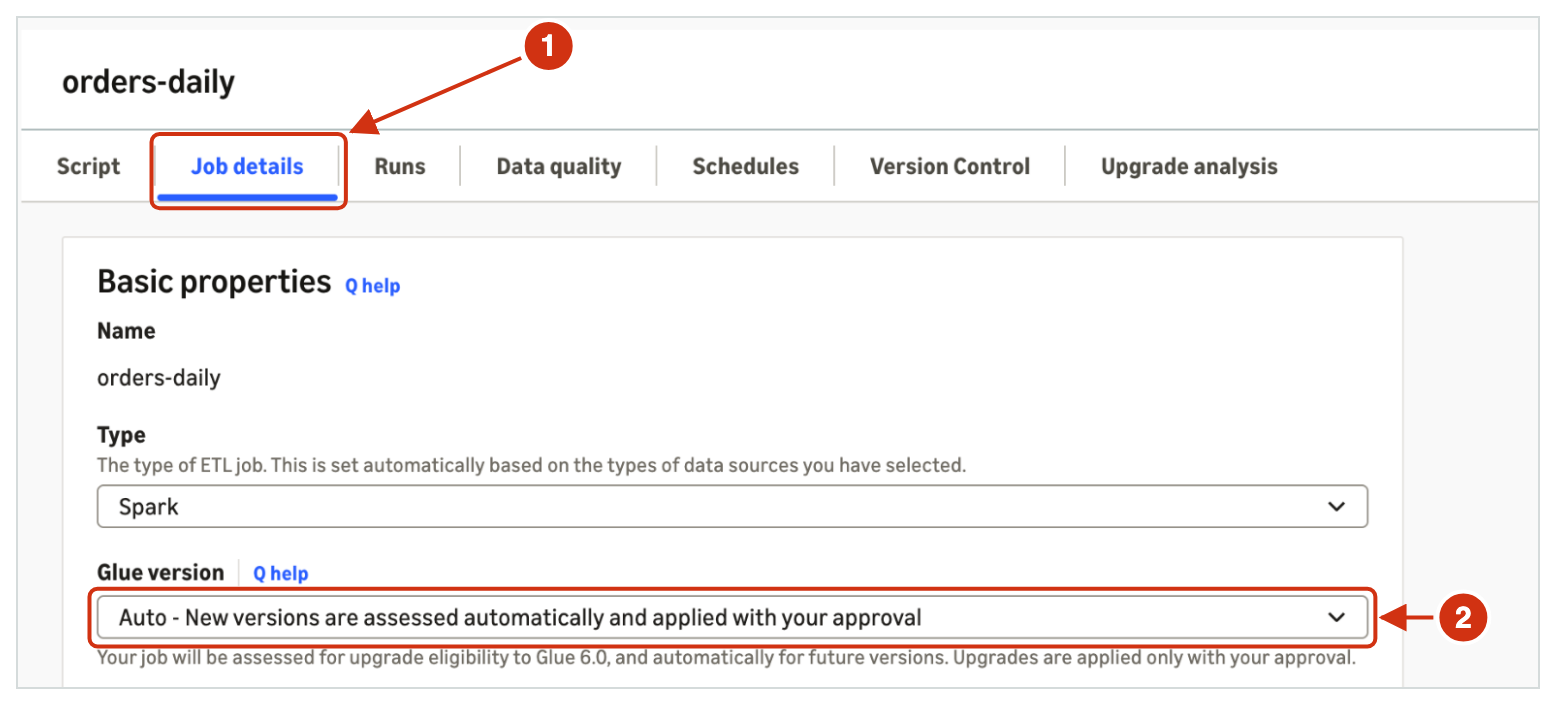
Choose the job, and then choose the Job details tab.
For AWS Glue version, choose Auto, and for Number of retries, enter 1 or higher.
Choose Save.
Figure 1: The Job details tab for orders-daily, with AWS Glue version set to Auto
Approve or decline the upgrade
When AWS Glue finishes the compatibility checks and finds no blocking issues, the job waits for your approval.
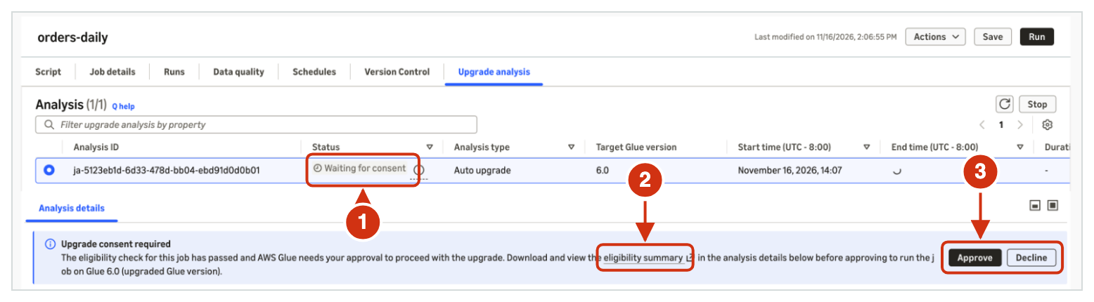
Choose the job, and then choose the Upgrade analysis tab. The analysis status shows Waiting for consent.
In the Upgrade consent required banner, choose eligibility summary, and review the summary.
Choose Approve to upgrade the job, or choose Decline to keep the job on its current version.
Figure 2: The Upgrade analysis tab for orders-daily, waiting for your approval
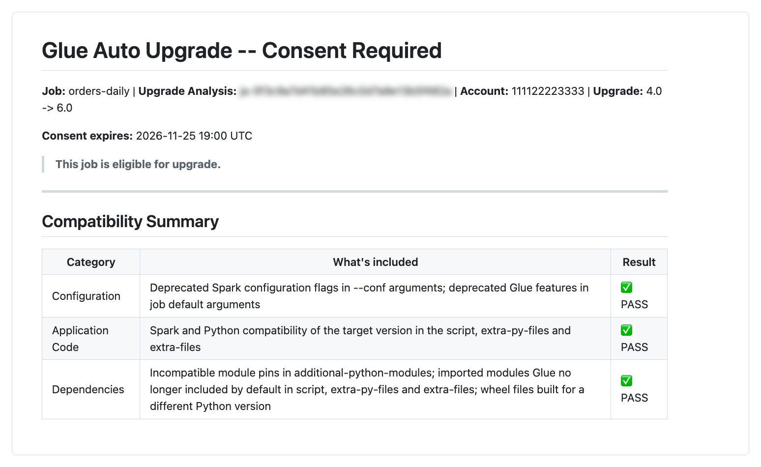
The eligibility summary shows the job, the AWS Glue versions, and the compatibility results.
Figure 3: The eligibility summary for orders-daily
Check the result
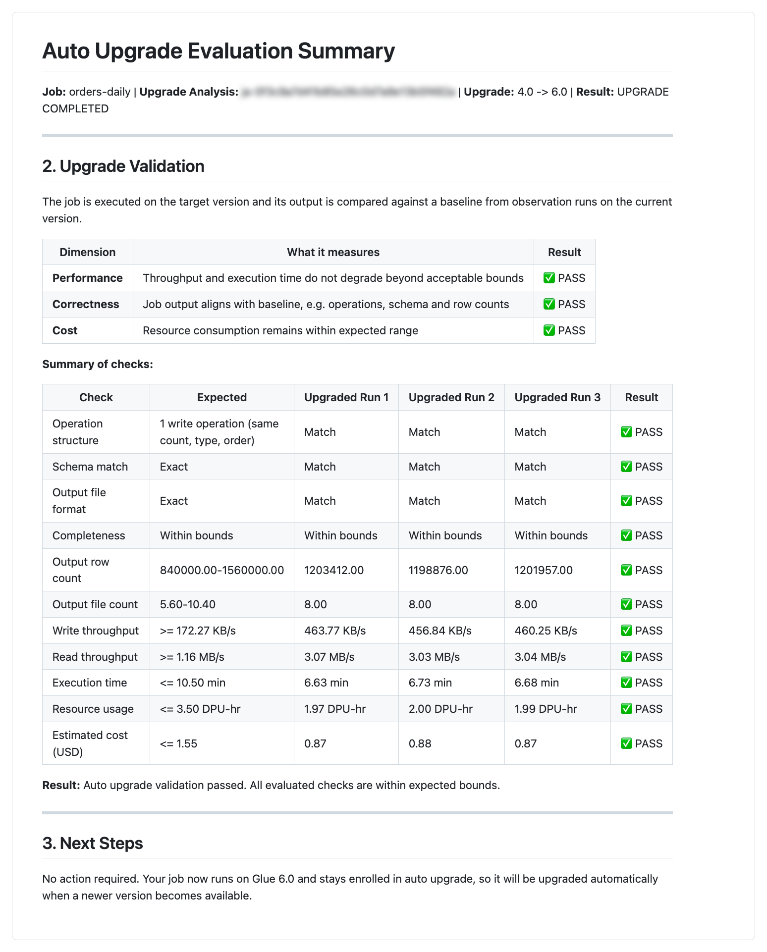
After the evaluation ends, the Upgrade analysis tab shows the auto upgrade evaluation summary. The summary shows the result for performance, correctness, and cost, with the expected range and each upgraded run’s value for every check.
Figure 4: The auto upgrade evaluation summary for orders-daily
Walkthrough: Upgrade a fleet of jobs with an AI agent
When you manage many jobs, an AI agent with the managing-glue-jobs skill assesses, turns on, and approves auto upgrade across your jobs from a few prompts. The agent shows each change and asks for your confirmation before it makes the change.
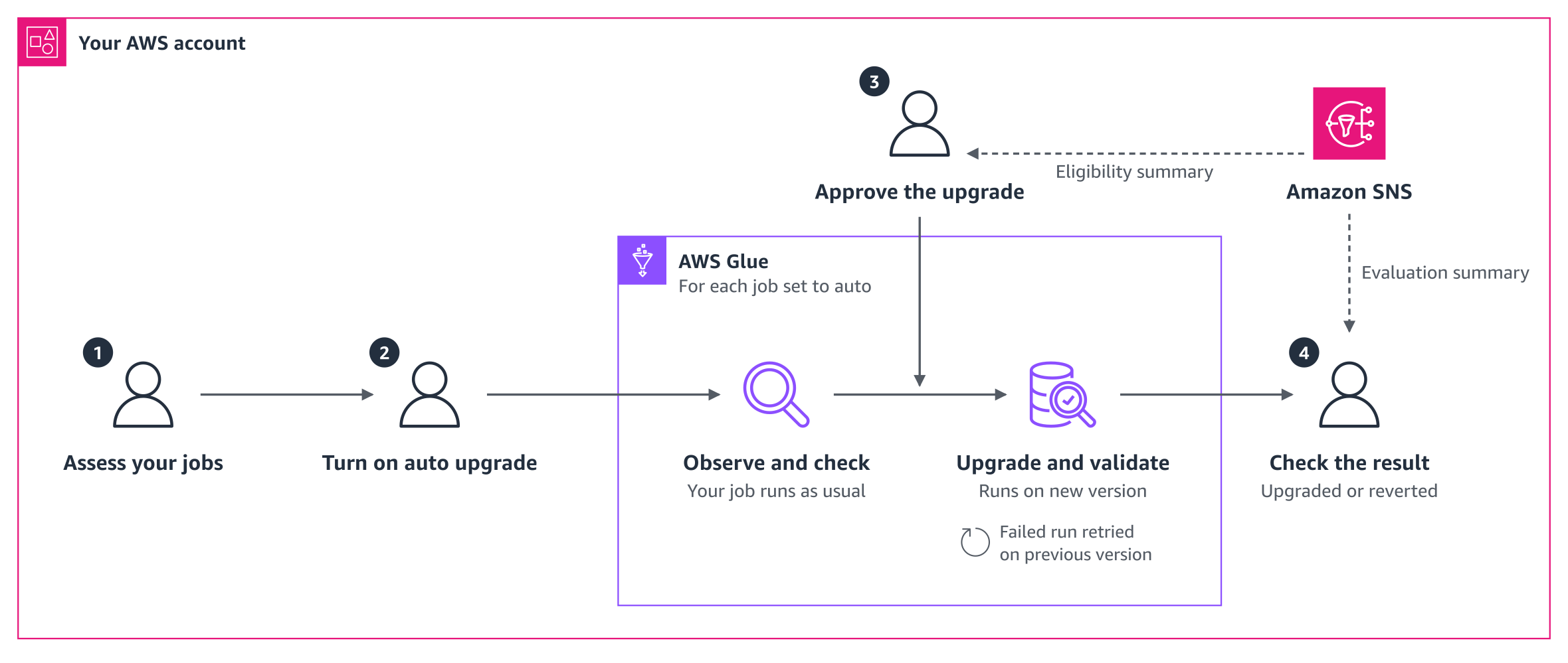
Figure 5: The auto upgrade journey for existing jobs
In this walkthrough, you assess your jobs, turn on auto upgrade, approve the upgrade, and check the result. Between these steps, AWS Glue observes and checks each job, and then upgrades and validates the job. Amazon SNS emails you the eligibility summary and the evaluation summary. The steps that follow match the numbers in Figure 5.
A data team runs three Spark ETL jobs in the US West (Oregon) Region and they want to use AWS Glue version 6.0. The jobs orders-daily and clickstream-agg run on AWS Glue 4.0 and write to Amazon Simple Storage Service (Amazon S3). The job customer-profiles runs on AWS Glue 3.0.
Step 1: Assess your jobs
Ask the agent which of your jobs can use auto upgrade. The assessment does not change anything in your environment, so it’s safe to try first. The agent checks each job against the requirements and runs a compatibility assessment. The agent then lists the jobs that can move to AWS Glue 6.0 and asks you to confirm that each job is safe to retry.
Figure 6: The agent assesses the jobs
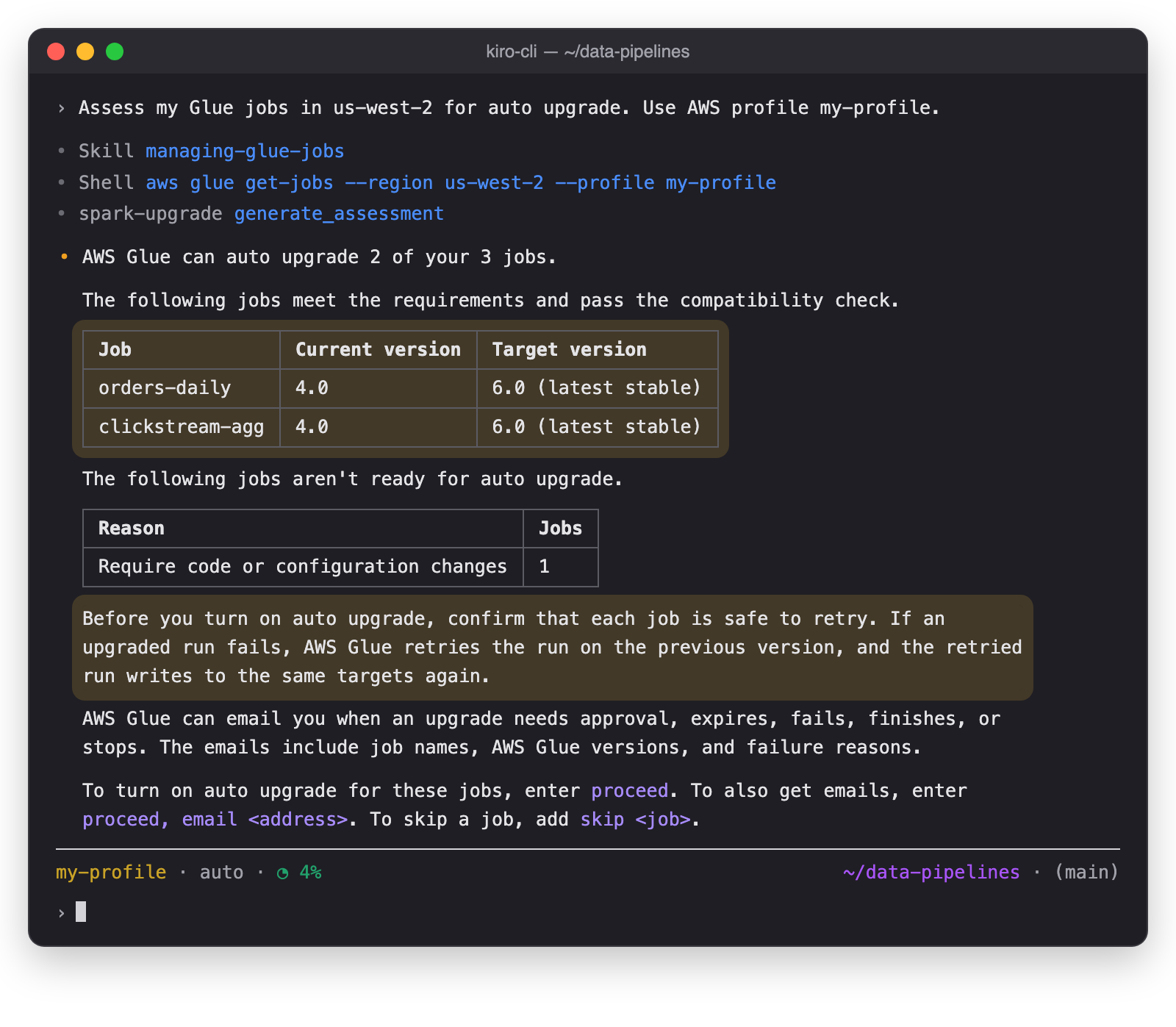
To see which job isn’t ready and why, ask the agent. The agent names the setting that blocks the upgrade and the fix.
Figure 7: The agent explains why a job isn’t ready
Step 2: Turn on auto upgrade and set up email notifications
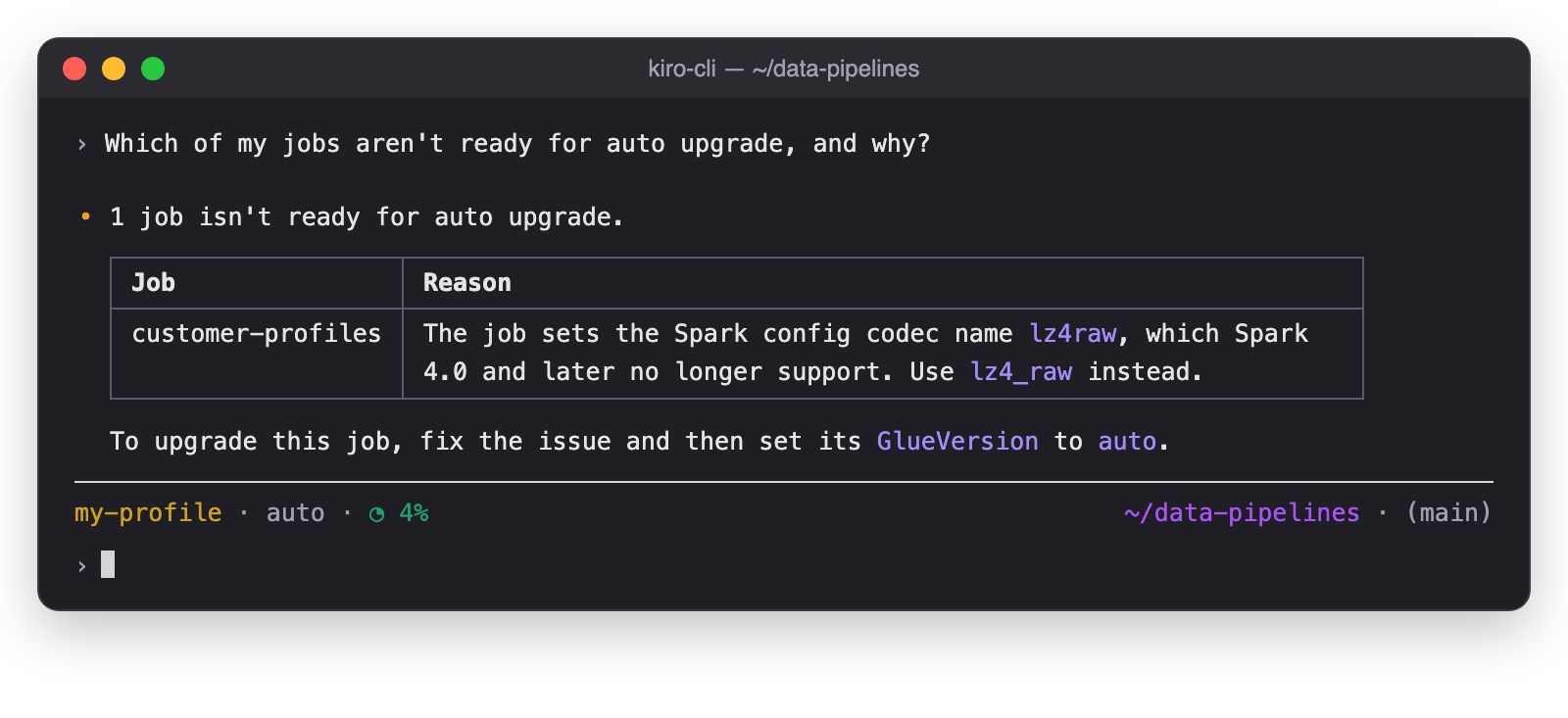
Ask the agent to turn on auto upgrade and set up email notifications in one prompt. The agent sets up the email notifications and sets GlueVersion to auto for each job. The jobs keep running on AWS Glue 4.0 until you approve an upgrade. To get the email notifications, confirm the subscription as the reply describes.
Figure 8: The agent turns on auto upgrade and sets up email notifications
Step 3: Review and approve the upgrade
AWS Glue observes and checks each job in the background, and then you review and approve the upgrade.
Step 3a: AWS Glue observes and checks
You keep running the jobs on their usual schedule. In the background, AWS Glue observes the runs and analyzes each job without changing it. How long this takes depends on how often each job runs.
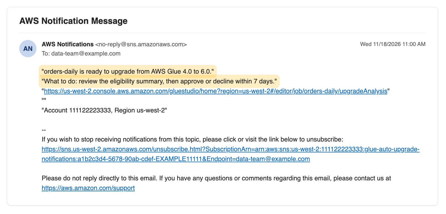
When a job is ready, AWS Glue emails you and requests your approval. The email names the job and the AWS Glue versions, and links to the job in the AWS Glue console. You have seven days to approve or decline.
Figure 9: The approval request email
Step 3b: Review and approve the upgrade
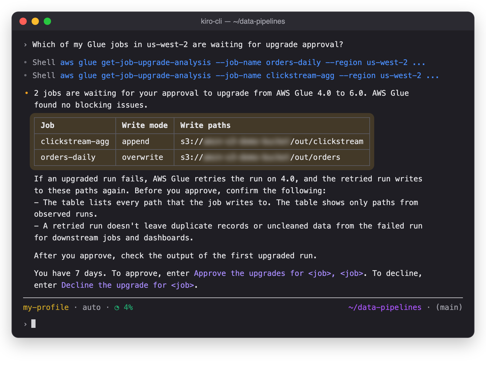
Ask the agent which upgrades are waiting. The agent reads the eligibility summary of each job, and then shows the jobs, their write paths, and what to confirm before you approve.
Figure 10: The agent shows the upgrades that wait for your approval
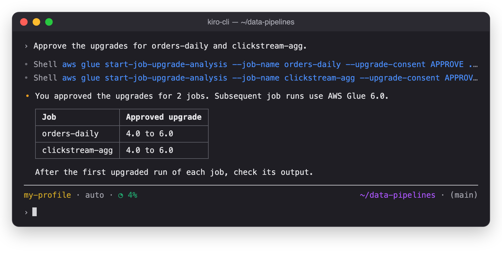
Before you approve, confirm that the reply lists every path that each job writes to. Then approve the jobs in one prompt, and name each job that you approve.
Figure 11: The agent approves the named jobs
The agent approves only the jobs that you name, and only jobs from the review that it showed you.
Step 4: Check the result
AWS Glue upgrades and validates each job, and then you check the result.
Step 4a: AWS Glue upgrades and validates
After you approve, subsequent runs of each job use AWS Glue 6.0, and AWS Glue validates the upgraded runs. If an upgraded run fails, AWS Glue retries the run on AWS Glue 4.0 and reverts the job. You don’t need to act in this step.
Step 4b: Check the result
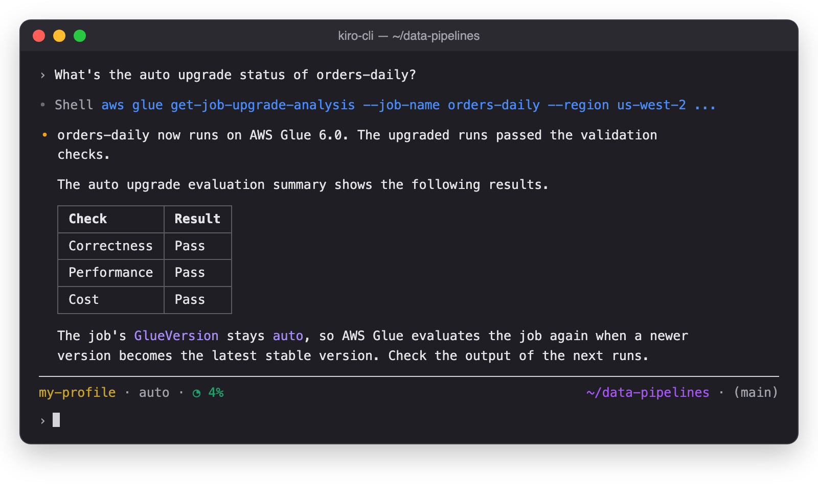
When the evaluation of a job ends, AWS Glue emails you the result. Ask the agent for the result of orders-daily. The agent shows the result of each validation check.
Figure 12: The agent shows the result for orders-daily
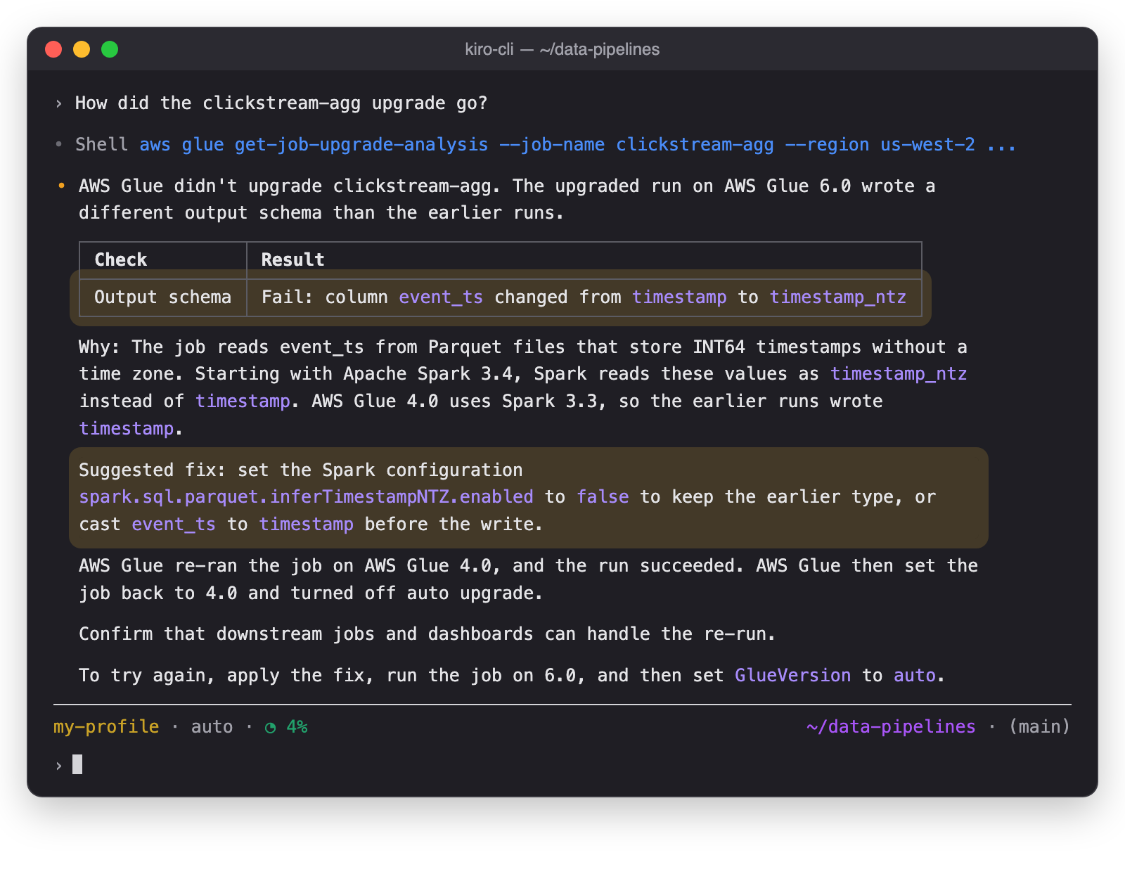
Ask the agent about the other job. The agent shows the check that failed and suggests a fix.
Figure 13: The agent explains why clickstream-agg didn’t upgrade
Your pipeline continues to run on AWS Glue 4.0. The auto upgrade evaluation summary shows what changed, so you can fix the job before you try again.
Conclusion
In this post, we showed how automatic version upgrades for AWS Glue jobs keep your Apache Spark jobs on the latest stable AWS Glue version. You used an AI agent to assess your jobs and turn on auto upgrade with email notifications. You then reviewed the eligibility summary, approved the upgrades, and checked the results in the auto upgrade evaluation summary.
With auto upgrade, your team no longer needs to plan and run an upgrade project for each job. AWS Glue analyzes each job and checks the upgraded runs against the job’s earlier runs. Your team reviews and approves each upgrade. This way you keep your whole fleet of AWS Glue jobs current instead of upgrading one job at a time.
Some jobs need code changes before they can move to a new version. For those jobs, use generative AI upgrades for Apache Spark in AWS Glue, which proposes and validates the code changes for the new version. After you update the code, set the job’s GlueVersion to auto so that AWS Glue keeps the job current from then on.
Auto upgrade is available today in all commercial AWS Regions. For the list of Regions, see Considerations and limitations in the AWS Glue User Guide. To get started, ask an AI agent with the managing-glue-jobs skill to assess the AWS Glue jobs in your account. Try auto upgrade, and share your feedback in the comments.
Special thanks
A special thanks to everyone who contributed from Engineering and Science to the launch of automatic version upgrades: Ezgi Maden, Akshara Ganapathi, Tina Shao, Raghavendhar Thiruvoipadi Vidyasagar, Shoukat Ghouse, David Zhang, Suthan Phillips, Prasad Nadig, Syed Mahmood, Karthik Seshadri, Pradeep Kumar Nalluri, Adam Rohrscheib, Eric Zhang, Tayo Adedokun, Weston Dunn, Kartik Panjabi, Shubham Mehta, Bryan Liles, Steffen Rochel, Kinshuk Pahare, Paul Meighan, and Rick Sears
You’ve turned on credit pooling, or you’re about to, and now the decisions are yours: how many seats to keep, how many additional credits to buy, and what limit each developer gets. Set limits too tight and developers get blocked in the middle of a task. Set them too loose and one runaway automation job can drain the pool and pause Kiro for everyone. The data to make these calls is already in your AWS account, in your Kiro user activity reports. This post shows you how to read it.
The launch post, Share Kiro credits across your team with credit pooling, published November 4, 2026, introduced credit pooling: a shared pool of Kiro credits that every user in the pool draws from. Credits one developer doesn’t need automatically become available to a teammate who does.
Credit pooling is for organizations. It works with Kiro profiles that use AWS IAM Identity Center, Okta, or Microsoft Entra ID. Individual Kiro subscriptions, such as a personal account with a social login, can’t share credits through a pool, and credit pooling isn’t available in AWS GovCloud (US).
This post is a hands-on guide for admins. It describes how the credit pool behaves day to day and how to size it and dial in your limit settings from your own usage data. It also covers the best practices that keep it running smoothly.
How credit pooling works
In credit pooling, a seat is one user’s access to the pool, and each seat adds 500 monthly credits. When someone leaves, removing them frees their seat for someone else. For details, see Manage seats.
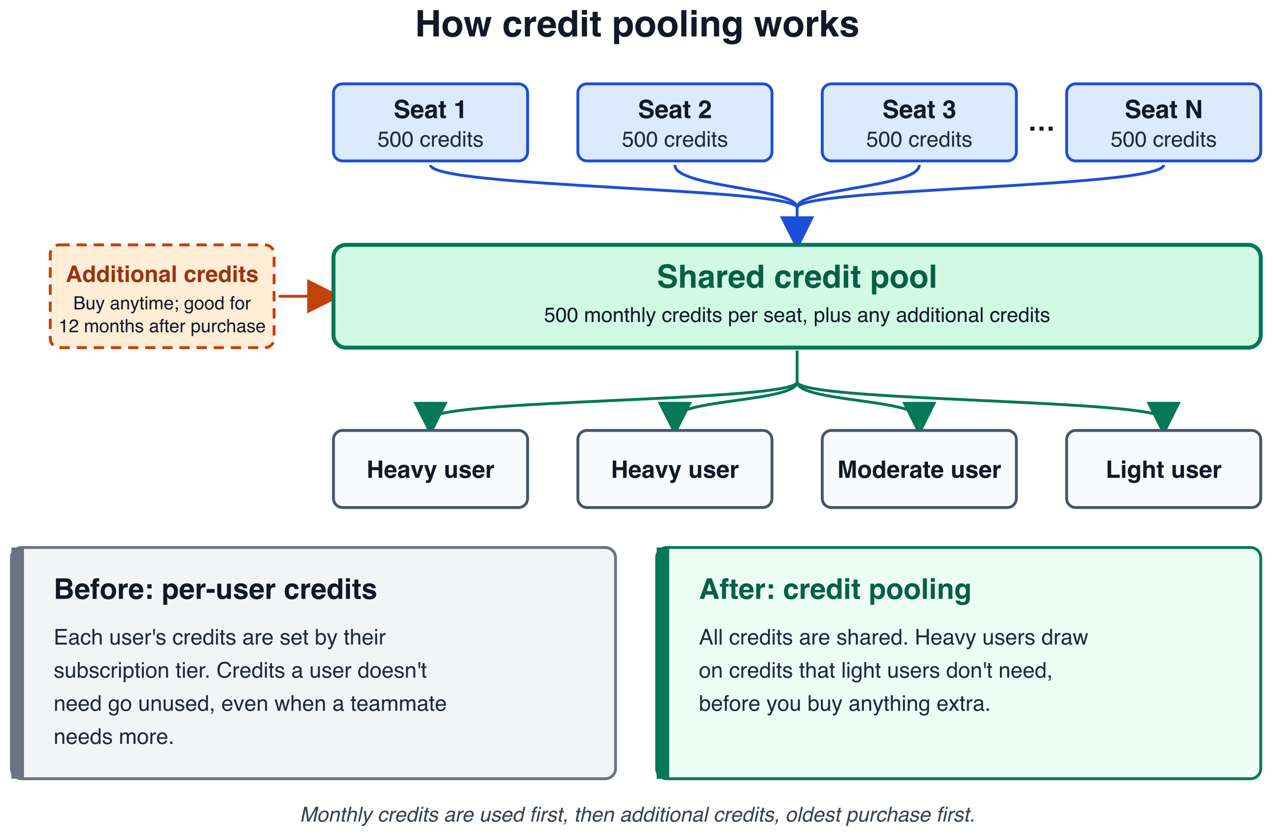
The following diagram shows how each seat’s 500 monthly credit inclusion flows into one shared pool, together with any additional credits you buy, and how every user draws from that pool. It also compares pooling with per-user credits.
Figure 1: How each seat’s 500 monthly credits flow into one shared pool that every user draws from, compared with per-user credits
Here’s a short summary of the core mechanics and how they play out once your pool is running. Each billing cycle, every $20 seat adds 500 credits to the pool, so 100 seats add 50,000. Every seated user draws from the pool, including users that run Kiro in headless mode, such as continuous integration and continuous delivery (CI/CD) pipelines. These credits continue to reset at the end of each billing cycle, but now they’re available for anyone in the pool to use.
When the pool runs out
Admins can buy additional credits at any time in the Kiro console. Additional credits roll over and are good for 12 months after purchase.
Which credits are used first
Monthly credits are used first because they reset at the end of each billing cycle. After the monthly credits run out, Kiro draws from additional credits, starting with the oldest purchase.
Where the savings come from
Credit pooling can help you save in three ways:
Shared credits absorb uneven usage. Your heaviest users draw on credits teammates don’t need before you buy anything extra.
Seats follow your team. Add seats as people join, and remove a user to release their seat when they leave.
Additional credits only when you need them. Buy them at any time, and they roll over for 12 months.
Walkthrough
Today, all you have is a daily report of each user’s consumption. This walkthrough turns that report into a plan in four steps. Step 1 loads the reports into Amazon Athena. Step 2 shows how each month used the pool. Step 3 recommends a seat count and a buffer of additional credits. Step 4 suggests a limit for each user.
Prerequisites
Before you start, confirm that the following are in place.
User activity reports turned on for your Kiro profile. The analysis in this post is based on the daily user activity CSV reports that Kiro writes to an Amazon Simple Storage Service (Amazon S3) bucket. To set them up, including the bucket policy Kiro needs to write to the bucket, see Turn on the CSV report.
Access to Amazon Athena, with permission to read the report location and write query results. For example, attach the AWS managed policy AmazonAthenaFullAccess, and allow s3:GetObject and s3:ListBucket on your report bucket.
The number of seats you bought for a prepaid pool, or the number of users in a postpaid pool. You manage seats under Access management > Credit sharing in the Kiro console. The activity report can’t give you this number.
An administrator role with the credit pooling permissions, so you can change seats, limits, and additional credits after the analysis.
Right-size your pool from your usage data
Your per-user activity reports record each user’s consumption.
Where to start depends on whether you already have data. If your team already uses Kiro, the activity report has recorded every user’s consumption all along, and the following queries run on that history as-is. Run Steps 2 and 3 now, before you pick a seat count. Step 3 tells you what that count needs to be.
If you are new to Kiro, there is nothing to analyze. Buy one seat for each person who needs access. That is the license, and the pool follows from it at 500 credits per seat. Keep a small buffer of additional credits (best practice 4), and start with generous limits (best practice 2). Either way, run one full billing cycle on pooling and come back to Step 2.
Step 1: Create the table and view
In the LOCATION line, replace the four capitalized placeholders. Use the Amazon S3 location you chose when you turned on the CSV report.
YOUR-BUCKET: the bucket name from your Amazon S3 location, for example amzn-s3-demo-bucket.
YOUR-PREFIX: the folder after the bucket name, for example user-activity-reports.
ACCOUNT-ID: the 12-digit AWS account where your users are subscribed.
REGION: the Region where you installed your Kiro profile, for example the US East (N. Virginia) Region (us-east-1).
For example, if your S3 location is s3://amzn-s3-demo-bucket/user-activity-reports/, the LOCATION line becomes s3://amzn-s3-demo-bucket/user-activity-reports/AWSLogs/111122223333/KiroLogs/user_report/us-east-1/. Keep the AWSLogs/.../KiroLogs/user_report/ part exactly as written. Kiro creates those folders itself.
Then create the view that the queries in the next steps read from:
CREATE OR REPLACE VIEW kiro_user_activity AS
WITH headers AS (
-- The first row of each report file names its columns.
SELECT "$path" AS report_file,
ARRAY[c1, c2, c3, c4, c5, c6, c7, c8, c9, c10,
c11, c12, c13, c14, c15, c16, c17, c18, c19, c20] AS names
FROM kiro_user_activity_raw
WHERE c1 = 'Date'
),
report_rows AS (
SELECT "$path" AS report_file,
ARRAY[c1, c2, c3, c4, c5, c6, c7, c8, c9, c10,
c11, c12, c13, c14, c15, c16, c17, c18, c19, c20] AS vals
FROM kiro_user_activity_raw
WHERE c1 <> 'Date'
)
-- Pick each value by its column name in that file's header.
-- A column the file doesn't have comes back NULL.
SELECT TRY(vals[array_position(names, 'Date')]) AS report_date,
TRY(vals[array_position(names, 'UserId')]) AS user_id,
TRY(vals[array_position(names, 'Client_Type')]) AS client_type,
TRY(vals[array_position(names, 'Credits_Used')]) AS credits_used,
TRY(vals[array_position(names, 'User_Email')]) AS user_email,
TRY(vals[array_position(names, 'Usage_Limit')]) AS usage_limit,
TRY(vals[array_position(names, 'Subscription_Tier')]) AS subscription_tier
FROM report_rows
JOIN headers USING (report_file);
Three details in that setup are worth knowing:
OpenCSVSerde, not ROW FORMAT DELIMITED. Kiro quotes some fields, and the simpler row format leaves the quote marks on, which breaks any join on user id.
The view finds columns by name, not position. Kiro has added columns to the report over time, so a position can hold a different column in an older file. The view reads each file’s header row and picks values by name. A column a file doesn’t have, like usage_limit in older reports, comes back empty.
The table reads the first 20 columns, all as text. They must be text, because the first row of each file holds column names. Everything the queries use is within the first 14 columns, and anything past 20 is ignored. If a column the queries need ever moves past 20, add c21 and up to both the table and the view.
Confirm it worked before going further:
SELECT COUNT(DISTINCT user_id) AS users,
ROUND(SUM(CAST(credits_used AS DOUBLE)), 2) AS credits,
MIN(report_date) AS first_day,
MAX(report_date) AS last_day
FROM kiro_user_activity;
For an example 100-seat team with six months of reports, that returns:
If that returns zero users, the LOCATION prefix is wrong. If user_id values come back wrapped in quote marks, the table was created with ROW FORMAT DELIMITED.
Step 2: Re-run every cycle and let the data correct your estimate
This is the query you come back to each cycle. It returns one row per closed month at today’s seat count, so one run shows your whole history. Change only the seat count. It answers the right-sizing question directly: at the seats I pay for now, which months overflow the pool, and how much sat unused?
WITH
-- ========================= EDIT ME =========================
inputs AS (
SELECT 100 AS seats -- the seats you pay for today, from the console
),
-- ======================= END EDIT ME =======================

-- Closed months only: the current month is not a full billing cycle yet.
per_user_month AS (
SELECT substr(a.report_date, 1, 7) AS month,
a.user_id,
SUM(CAST(a.credits_used AS DOUBLE)) AS credits
FROM kiro_user_activity a
WHERE date(a.report_date) < date_trunc('month', current_date)
GROUP BY substr(a.report_date, 1, 7), a.user_id
),

totals AS (
SELECT month,
COUNT(*) AS active_users,
SUM(credits) AS consumed,
SUM(GREATEST(credits - 500.0, 0)) AS beyond_own_seat,
approx_percentile(credits, 0.50) AS p50,
approx_percentile(credits, 0.90) AS p90,
MAX(credits) AS max_user
FROM per_user_month
GROUP BY month
)

SELECT
t.month,
i.seats,
t.active_users,
GREATEST(i.seats - t.active_users, 0) AS seats_never_used,
ROUND(t.consumed, 0) AS credits_consumed,
ROUND(GREATEST(i.seats * 500.0 - t.consumed, 0), 0) AS pool_credits_unused,
ROUND(GREATEST(i.seats * 500.0 - t.consumed, 0) * 0.04, 2) AS unused_credit_value_usd,
ROUND(t.beyond_own_seat
- GREATEST(t.consumed - i.seats * 500.0, 0), 0) AS credits_covered_by_sharing,
ROUND(GREATEST(t.consumed - i.seats * 500.0, 0), 0) AS additional_credits_needed,
ROUND(i.seats * 20.0
+ GREATEST(t.consumed - i.seats * 500.0, 0) * 0.04, 2) AS estimated_monthly_cost,
ROUND(t.active_users * 20.0
+ GREATEST(t.consumed - t.active_users * 500.0, 0) * 0.04, 2)
AS cost_if_never_used_seats_reclaimed,
ROUND(t.p90, 0) AS p90_credits_per_user,
ROUND(t.max_user, 0) AS max_credits_per_user
FROM totals t CROSS JOIN inputs i
ORDER BY t.month;
Sample output for the same team, one column per closed month. The current month is left out because it isn’t a full cycle:
For this team, credits that light users didn’t need covered 7,654 to 13,816 credits of heavier users’ demand every month, so it never bought additional credits. That’s how pooling can work. Even so, 2,000 to 11,700 credits went unused each month and 11 to 21 seats sat idle, which Step 3 turns into a plan.
Read it across, not down. If pool_credits_unused stays large for a couple of cycles, the seats behind it are not a one-off. Reclaim them from people who no longer need access and re-run next month to confirm.
If additional_credits_needed is climbing, buy additional credits earlier in the cycle rather than adding seats (see best practice 7). credits_covered_by_sharing, multiplied by $0.04, estimates what sharing saved you each month. When p90_credits_per_user and max_credits_per_user settle into a stable range, that is your signal to set limits with headroom above them.
seats_never_used counts seats with no activity that month, and cost_if_never_used_seats_reclaimed is your cost if you reclaimed them all. Treat it as a bound, not a target. Step 3 looks across several months before it recommends cuts.
The percentiles are your starting point for limits. p90_credits_per_user reflects your heavy users, and max_credits_per_user is the person who reaches a limit first. With fewer than a few dozen active users, lean on max. Step 4 suggests a limit for each person.
Step 3: Turn the numbers into a resizing plan
Step 2 shows what happened. This query turns that into a plan: seats to keep and reclaim, additional credits to hold, and what the change saves. In the EDIT ME block, set your seat count and how many closed months to look back over. Three months is a sensible default, because one quiet month doesn’t mean a seat is unneeded.
WITH
-- ========================= EDIT ME =========================
inputs AS (
SELECT 100 AS seats, -- the seats you pay for today, from the console
3 AS lookback_months -- closed months to base the plan on
),
-- ======================= END EDIT ME =======================

bounds AS (
SELECT i.seats,
date_trunc('month', current_date) AS this_month,
date_add('month', -i.lookback_months,
date_trunc('month', current_date)) AS since
FROM inputs i
),

-- Everyone who used Kiro since the window started, this month included,
-- needs a seat. Seats nobody used in that time are the ones to reclaim.
users AS (
SELECT COUNT(DISTINCT a.user_id) AS active_users
FROM kiro_user_activity a
CROSS JOIN bounds b
WHERE date(a.report_date) >= b.since
),

-- Credits consumed in each closed month of the window.
months AS (
SELECT substr(a.report_date, 1, 7) AS month,
SUM(CAST(a.credits_used AS DOUBLE)) AS consumed
FROM kiro_user_activity a
CROSS JOIN bounds b
WHERE date(a.report_date) >= b.since
AND date(a.report_date) < b.this_month
GROUP BY substr(a.report_date, 1, 7)
),

-- Never recommend more seats than you have, so every result stays sensible.
sized AS (
SELECT b.seats,
u.active_users,
LEAST(b.seats, u.active_users) AS rec
FROM bounds b
CROSS JOIN users u
),

-- Each window month at today's seats and at the recommended seats, with
-- anything past the pool bought as additional credits.
plan AS (
SELECT s.seats,
s.active_users,
s.rec,
MAX(m.consumed) AS busiest,
AVG(s.seats * 20.0
+ GREATEST(m.consumed - s.seats * 500.0, 0) * 0.04) AS cost_now,
AVG(s.rec * 20.0
+ GREATEST(m.consumed - s.rec * 500.0, 0) * 0.04) AS cost_resized
FROM sized s
CROSS JOIN months m
GROUP BY s.seats, s.active_users, s.rec
)

SELECT
seats,
active_users AS active_users_in_window,
rec AS recommended_seats,
seats - rec AS seats_to_reclaim,
ROUND(busiest, 0) AS busiest_month_credits,
rec * 500 AS recommended_pool_credits,
ROUND(GREATEST(busiest - rec * 500.0, 0), 0) AS additional_credits_to_keep,
ROUND(cost_now, 2) AS avg_monthly_cost_now,
ROUND(cost_resized, 2) AS avg_monthly_cost_resized,
ROUND(cost_now - cost_resized, 2) AS avg_monthly_savings
FROM plan;
Sample output for the same team at 100 seats, looking back over July through September:
recommended_seats is one seat for everyone who used Kiro in the lookback or so far this month, however lightly, and seats_to_reclaim is the rest. The report can’t tell you who joined last week or is on leave, so check the names in the Kiro console before you reclaim anything.
additional_credits_to_keep is how far your busiest month ran past the recommended pool. Keep at least that many additional credits on hand going into each cycle (best practice 4). That’s a balance to hold, not an amount to buy every month, so check what’s already in your pool on the Kiro dashboard and buy only the difference. If Step 2 shows consumption climbing, keep more than this.
The cost columns compare the lookback months at your current seats with their cost at the recommended seats, averaged per month. Each month costs $20 per seat plus $0.04 per credit used beyond the pool, counted in the month it’s used. For this example team, reclaiming 14 idle seats would save about $213.30 a month on average, roughly $2,600 a year if the pattern holds. In July, the busiest month, about $200 of the $280 in seat savings came back as additional credits, which is why the buffer matters.
Step 4: Find users whose limits need to change
Seats and the pool are half of right-sizing. Per-user limits are the other half. This query lists the people whose limit is out of step with what they use. It flags anyone whose busiest month in the lookback reached 80% of their limit, anyone who stayed under 25% of their limit every month, and anyone with no limit set. For each one it suggests a new limit: their busiest month plus 25%, rounded up to the nearest 100 and never below the 500 credits a seat adds to the pool. It only lowers limits for people active in every month of the lookback, so a new joiner isn’t cut after one quiet month. Adjust the thresholds in the EDIT ME block.
WITH
-- ========================= EDIT ME =========================
inputs AS (
SELECT 3 AS lookback_months, -- closed months to look back over
0.80 AS raise_at, -- raise if the busiest month reached 80% of the limit
0.25 AS lower_below, -- lower if every month stayed under 25% of the limit
1.25 AS headroom -- new limit = busiest month plus 25%
),
-- ======================= END EDIT ME =======================

bounds AS (
SELECT date_add('month', -i.lookback_months,
date_trunc('month', current_date)) AS since
FROM inputs i
),

-- Credits per user in each month of the window, this month so far included,
-- so a suggested limit is never below what someone has already used.
per_user_month AS (
SELECT a.user_id,
substr(a.report_date, 1, 7) AS month,
ROUND(SUM(CAST(a.credits_used AS DOUBLE)), 2) AS credits
FROM kiro_user_activity a
CROSS JOIN bounds b
WHERE date(a.report_date) >= b.since
GROUP BY a.user_id, substr(a.report_date, 1, 7)
),

-- Each user's plan, limit and email from their most recent report. On a pool,
-- Usage_Limit is the pool limit (999999 means none is set). On a subscription
-- (Pro, Pro+, Pro Max, Power), it's the tier's monthly credit allowance.
-- If one day has both, the pool row wins. Older reports have no limit
-- column, so the view returns NULL and they're skipped.
latest AS (
SELECT a.user_id,
max_by(a.user_email, a.report_date || IF(upper(a.subscription_tier) = 'POOLING', '1', '0')) AS user_email,
max_by(replace(upper(a.subscription_tier), '_', ''),
a.report_date || IF(upper(a.subscription_tier) = 'POOLING', '1', '0')) AS plan,
max_by(TRY_CAST(a.usage_limit AS DOUBLE),
a.report_date || IF(upper(a.subscription_tier) = 'POOLING', '1', '0')) AS lim
FROM kiro_user_activity a
CROSS JOIN bounds b
WHERE date(a.report_date) >= b.since
AND a.usage_limit IS NOT NULL
AND COALESCE(a.subscription_tier, '') <> ''
GROUP BY a.user_id
),

-- Suggested limit: the busiest month plus headroom, rounded up to the
-- nearest 100, and never below the 500 credits one seat brings to the pool.
-- months_active counts the closed months in the lookback with any use.
scored AS (
SELECT l.user_email,
l.plan,
COALESCE(l.lim, 999999) AS lim,
MAX(m.credits) AS busiest,
COUNT_IF(m.month < date_format(current_date, '%Y-%m')) AS months_active,
GREATEST(ceiling(MAX(m.credits) * i.headroom / 100) * 100, 500) AS new_limit,
i.lookback_months,
i.raise_at,
i.lower_below
FROM per_user_month m
JOIN latest l ON m.user_id = l.user_id
CROSS JOIN inputs i
GROUP BY l.user_id, l.user_email, l.plan, l.lim,
i.lookback_months, i.headroom, i.raise_at, i.lower_below
),

-- Lower a limit only for someone who used Kiro in every closed month of the
-- lookback, so a new joiner or someone back from leave isn't cut after one
-- quiet month.
flagged AS (
SELECT *,
CASE
WHEN plan <> 'POOLING' THEN 'limit when pooled'
WHEN lim >= 999999 THEN 'set limit'
WHEN busiest >= raise_at * lim THEN 'raise'
WHEN busiest < lower_below * lim
AND new_limit < lim
AND months_active = lookback_months THEN 'lower'
END AS action
FROM scored
)

SELECT user_email,
CASE plan WHEN 'POOLING' THEN 'Pool' WHEN 'PRO' THEN 'Pro' WHEN 'PROPLUS' THEN 'Pro+'
WHEN 'PROMAX' THEN 'Pro Max' WHEN 'POWER' THEN 'Power' ELSE plan END AS plan,
CAST(ROUND(busiest) AS BIGINT) AS busiest_month,
IF(lim >= 999999, 'none',
CAST(CAST(lim AS BIGINT) AS VARCHAR)) AS usage_limit,
IF(lim >= 999999, NULL,
ROUND(100.0 * busiest / lim, 0)) AS pct_of_limit,
action,
CAST(new_limit AS BIGINT) AS new_limit
FROM flagged
WHERE action IS NOT NULL
ORDER BY CASE action WHEN 'raise' THEN 1 WHEN 'set limit' THEN 2 WHEN 'lower' THEN 3 ELSE 4 END,

user_email;
Sample output for the same team, looking back over July through October so far:
The raise rows are the people closest to being blocked. In their busiest month, user021 used 994 of their 1,000 credits, so one heavy week might stop them. Raising it to 1,300 gives them room. A higher limit adds no cost until the credits are used.
The lower rows are people who use a small share of their limit, like user006, whose busiest month was 513 credits against a 3,000-credit limit. Lowering a limit doesn’t save money, because a credit costs the same whoever uses it. It limits the impact of a runaway automation job, so one person is less likely to drain the pool and block everyone. new_limit is never below what the user has already used this month, so lowering it doesn’t block them right away.
The limit when pooled rows are people still on a Pro, Pro+, Pro Max, or Power subscription. Their usage_limit is the tier’s monthly allowance, so above 100% means they need more than their tier includes, like user091. new_limit is the individual limit to allocate when you add them to the pool. Their usage is already counted in Step 3’s additional_credits_to_keep, so the buffer covers them too.
If several people in one group need the same change, change the group’s limit.
For the exceptions, set new_limit as an individual limit in the Kiro console. It takes priority over group and profile limits (best practice 2). Re-run this query each cycle to catch limits that need to move again.
Best practices for making credit pooling effective
These practices build on the numbers from the walkthrough and help you keep the pool sized without blocking anyone.
1. Learn your usage pattern first
Collect several months of data before you fine-tune anything. A couple of billing cycles show you who your heavy and light users are, how usage rises and falls through a sprint, and how quickly the pool draws down. Once you can see the trend, use the preceding analysis to size the pool and set limits.
2. Use the limit hierarchy strategically
With credit pooling, you can set per-user limits at three levels:
Level
Priority
Use it for
Individual
Highest
Setting a per-user limit that applies to a specific user (for example, a user that runs automations, or someone testing heavily)
Group
Medium
Setting a per-user limit that applies to all members of a group
Profile
Lowest
Setting a default limit applicable to all users
All limits are per-user. There are no aggregate caps at the group or profile level. A group limit sets the per-user cap for everyone in that group.
Where to start: If your team already uses Kiro, start from the limits Step 4 suggests. If you are new to Kiro, start with generous group and profile limits and tighten them after your first billing cycle, only where the data shows you need to. Over-constraining on day one creates friction and support tickets.
3. Group users by usage pattern
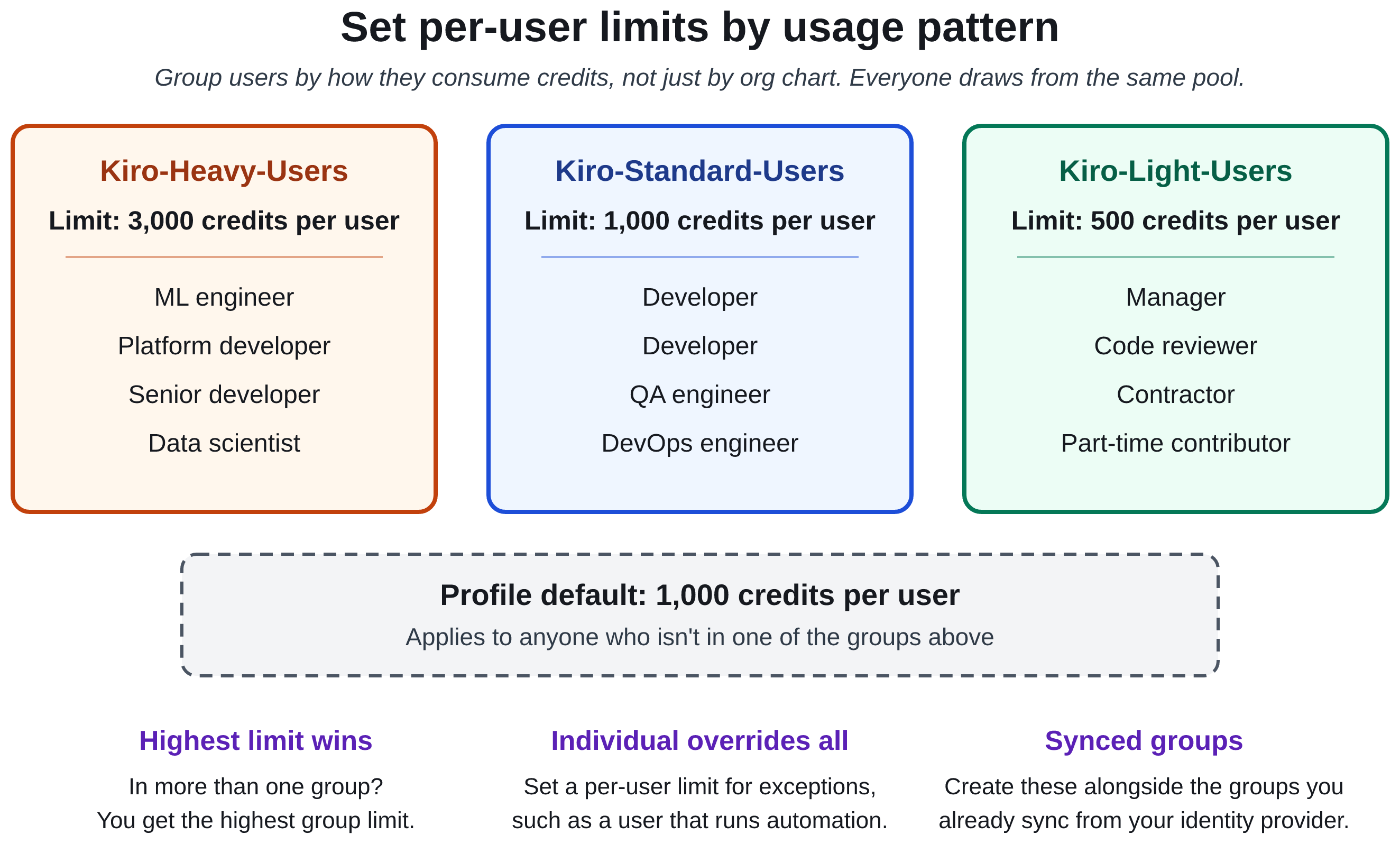
Consider grouping users by how they consume credits rather than only by org chart. For example, put heavy users (senior developers, machine learning engineers) in a group with a higher per-user limit, and light users (managers, reviewers) in a group with a lower one.
Figure 2: Grouping users by usage pattern to apply different per-user limits
If you sync groups from your identity provider: Your existing synced groups likely mirror your org chart. Create groups for credit pooling. For example, keep your synced “Engineering” group for access management, but create separate “Kiro-Heavy-Users” and “Kiro-Standard-Users” groups to apply different per-user limits. Users can belong to multiple groups, and the highest limit wins.
4. Keep a buffer of additional credits
When the pool is empty, everyone stops. Watch your pool threshold alerts and buy additional credits before the pool runs low. Because additional credits roll over for 12 months, buying early doesn’t waste them. Step 3’s additional_credits_to_keep shows how many to hold, based on your busiest month.
Daily projected consumption with run-out date predictions.
Credit usage breakdown (monthly compared to additional credits).
Users sharing credits, credits left, and additional credits at a glance.
If you exhaust the monthly pool early, buy additional credits earlier in the cycle. If credits go unused, check whether some seats are inactive (best practice 7).
6. Use notifications to stay ahead
Credit pooling includes built-in alerts that notify admins at 80% and 100% by default:
Pool threshold alerts: Get notified when the pool drops below configured levels.
User usage alerts: Know when individual users approach their limits.
Seat utilization alerts: Know when assigned seats near the number you bought.
Send these to the people who can act on them.
7. Right-size seats, and use credits rather than seats for headroom
A seat is an access license first and a credit contribution second. Treat them as two separate questions.
Seats with zero usage are the first place to look. You pay $20/month for a seat whether anyone signs in or not, and the seats_to_reclaim figure from Step 3 shows how many have gone unused for the whole lookback. Reclaim those from people who no longer need access.
Lightly used seats are a different matter. Don’t cut a license from someone who uses Kiro occasionally because their consumption is low. Their unused credits already go to the pool.
For headroom, buy credits rather than seats. If demand runs ahead of your pool, buy additional credits. Monthly credits reset at the end of the cycle. Additional credits last 12 months.
Things to keep in mind
When the pool runs out, usage stops for everyone in it. Kiro blocks further usage, whatever each user’s limit, until you add credits.
Mid-cycle limit changes take effect immediately. If you lower a user’s limit below their current consumption, they’re blocked right away. If you increase their limit, they can immediately resume their AI use. Plan limit changes at the start of a billing cycle when possible.
In a prepaid pool, seats are billed whether occupied or not. Every seat contributes credits and costs $20/month. Factor in your idle seats when calculating return on investment.
Getting started
If you have a Kiro profile with users signing in through single sign-on (SSO), you’re ready to go:
Switching is irreversible: a user you move can’t go back to an individual subscription. Have each user’s Step 4 limit ready to apply once they’re in the pool.
Key details at a glance
The following table summarizes the numbers and rules covered in this post.
Item
Detail
Credits per seat
500/month (shared)
Cost per seat
$20/month
Additional credits
$0.04 per credit, good for 12 months
Monthly credit reset
End of billing cycle
Consumption order
Monthly → Additional (oldest purchase first)
Limit hierarchy
Individual > Group > Profile
Start sharing
Credit pooling turns unused individual capacity into a shared resource. Teams with uneven usage can get more from the same spend, and limits at every level help you stay in control.
Ready to try it? Head to the Kiro console and turn on credit sharing under Access management. For details on seats, limits, and monitoring, see Credit pooling in the Kiro documentation.
Not every action a user takes in an application carries the same risk. Viewing an account balance in a banking application isn’t the same as wiring several thousand dollars to a new payee. In practice, though, many applications ask users to prove their identity once at sign-in and then treat every action the same from that point on, whether that sign-in used a password alone or included multi-factor authentication (MFA). That creates a tension: if the sign-in is strict enough for the most sensitive operation, everyday tasks carry unnecessary friction. If it’s easy enough for everyday tasks, the most sensitive operations might not be protected well enough. Even a strong sign-in from hours earlier says little about who is at the keyboard when a high-risk request arrives.
Amazon Cognito now resolves that trade-off by supporting step-up authentication, which records the authentication assurance level and the methods used, and including both in the JSON web tokens (JWTs) it issues. You ask for a target assurance level when a user signs in. Amazon Cognito returns the level the user reached in an acr claim (authentication context class reference) and the methods they completed in an amr claim (authentication methods reference). These claims are part of the OpenID Connect Core specification, so your application can reason about authentication strength in a standard way and match it to the potential risk of what the user is trying to do. In this post, I explain how the claims support step-up authentication and walk through four patterns that put them to use: transaction-level step-up in a banking app, varying risk postures across a portfolio of applications, step-up enforced on API and SDK sign-in, and authentication assurance carried across a federated third-party OpenID Connect (OIDC) identity provider.
You can request authentication levels through Amazon Cognito managed login using the standard OIDC acr_values and max_age parameters, and through the SDK and API using the USER_AUTH flow with TARGET_ACR_VALUES and MAX_AGE. Requesting step-up authentication requires the Essentials or Plus feature plan. ; For the complete list of features, behaviors, and limitations, see the Authentication levels with ACR and AMR claims.
What ACR and AMR tell your application
Amazon Cognito defines four assurance levels, and the factor combinations that satisfy each one are fixed. You can use the default names as is or rename the level URIs to fit your organization’s own naming scheme. Renaming changes only the label. If you need to relate Amazon Cognito levels to a framework such as NIST SP 800-63 or eIDAS, make that mapping in your application. The following are the default Amazon Cognito defined levels.
Level 1 (urn:cognito:loa:1) is password only.
Level 2 (urn:cognito:loa:2) is a single one-time password (OTP) over SMS or email.
Level 3 (urn:cognito:loa:3) is a passkey on its own, or a password combined with an SMS or email OTP.
Level 4 (urn:cognito:loa:4) is the highest: a password with a time-based one-time password (TOTP) code from an authenticator app.
Amazon Cognito assigns the highest level the user’s completed factors fully satisfy, so a user who signs in with a password and a TOTP code lands at level 4, even though they also met the assurance requirements for every level below it.
Four claims in the token facilitate a step-up decision. The acr claim is the level the sign-in reached and is what your application compares against what the operation requires. The amr claim lists the methods behind that level, so you can confirm a specific factor was used. The auth_time claim records when the user last authenticated interactively and is what max_age is measured against. The iat claim only records when the token was issued, so a refreshed token carries a new iat but keeps its old auth_time. Finally, send a nonce in the request and verify it on the returned ID token, so the result is tied to the request you made.
The following is an example access token for a user completing a level 4 authentication. Notice the four claims I’ve discussed: acr, amr, auth_time, and iat.
Two important behaviors are worth understanding before you build on this. First, a token refresh preserves the acr and amr values, so a user who reached level 4 keeps level 4 across refreshes and isn’t asked to prove it again on every rotation. Second, a refresh doesn’t reset the auth_time claim. That field records when the user interactively authenticated, not from a non-interactive token refresh. This is what lets you reason about freshness of authentication separately from assurance strength.
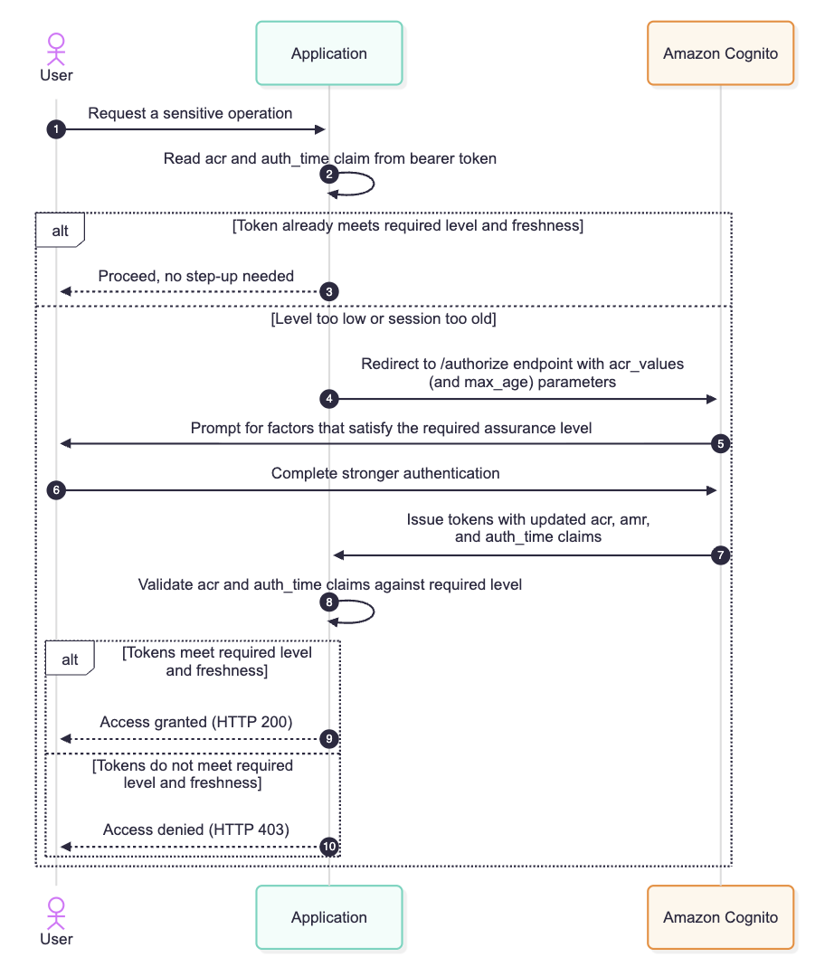
At a high level, every step-up interaction in this post follows the same loop: the application checks the token it already holds, redirects for a stronger level only when the operation requires more than the user has, and re-validates the acr claim on the freshly issued token before it proceeds. The following diagram provides a general step-up authentication flow.
Figure 1: General step-up authentication flow to access a sensitive operation
How you request a level, and what stays your responsibility
The request side is deliberately straightforward. On managed login you add acr_values and optionally max_age to the or endpoint. In the SDK and API, you pass TARGET_ACR_VALUES and MAX_AGE in the USER_AUTH flow of the API. Both acr_values and TARGET_ACR_VALUES accept an ordered list of target levels. The same parameters work whether you’re setting the level for an initial sign-in or raising the level of a user who is already signed in; the patterns later in this post show both. Amazon Cognito acts only on what you send. It doesn’t infer the level you meant, so if you omit the parameter or request the wrong level, the user might not be stepped up the way you intended.
That points to the part your application and API owns: what assurance authentication level is needed. Amazon Cognito issues a token that honestly reports the level the user reached based on what your application requested. For example, deciding that a given operation requires an assurance level 3, checking the token’s acr against that requirement, and refusing the operation when it falls short is enforcement your application and API performs. Amazon Cognito produces the evidence; your code acts on it. In practice, that means checking the token you already hold before you redirect, so you don’t send a user to re-authenticate who already meets the bar, and validating the acr and auth_time claims on the tokens Amazon Cognito returns before you grant access. Amazon Cognito computes these claims itself, so you can’t customize, add to, or suppress them with a pre-token-generation Lambda trigger.
There is one more detail that saves debugging time later. If you rename your acr level URIs after tokens have already been issued, an older token might carry an acr value that no longer matches any configured level. Amazon Cognito treats that as an unrecognized level rather than an error. It still honors the token’s amr values and prompts only for factors not already present, without crediting any particular level. The amr list, in other words, remains meaningful even when a renamed level string goes stale. See Configuring ACR level names to learn how to configure this.
With the claims and the division of responsibility in place, the following four patterns show how they work in practice. Each one applies the same loop from Figure 1 to a different situation: a single application, a portfolio of applications, API-driven sign-in, and federation.
Pattern 1: Transaction-level step-up in a banking app
Consider a retail banking application. Signing in and viewing balances is routine, and the bank is comfortable requiring a moderate assurance level for it. Moving money is considered a privileged action, and a large transfer deserves stronger proof that the person at the keyboard is really the account holder.
The bank sets its baseline at level 2, so a user signs in with a one-time code over SMS or email and can see balances, statements, and pending transactions. When that same user initiates a transfer above $1,000, the application’s own policy says the operation requires level 4. Before it shows the transfer initiation screen, the application inspects the acr claim in the token it already holds. The user authenticated at level 2, level 2 is below the required level 4, so the application redirects the user to managed login with acr_values=urn:cognito:loa:4.
GET https://auth.example-bank.com/oauth2/authorize
    ?response_type=code
    &client_id=abc123def456
    &redirect_uri=https://app.example-bank.com/callback
    &scope=openid
    &acr_values=urn:cognito:loa:4
Amazon Cognito now requires the user to complete a factor combination that satisfies level 4, for example entering their password and then a TOTP code from their authenticator app. When authentication finishes, Amazon Cognito issues fresh tokens with acr set to urn:cognito:loa:4, amr set to ["pwd", "otp", "mfa"], and a fresh updated auth_time claim. The application validates that the new token meets its requirement and only then lets the transfer proceed. A transfer under the threshold never triggers any of this, so the everyday experience stays light and the friction lands exactly where the risk is.
The application logic reads naturally, here’s a pseudo JavaScript snippet:
// Use your own URIs here, if different than defaults.
const ACR_RANK = {
  "urn:cognito:loa:1": 1,
  "urn:cognito:loa:2": 2,
  "urn:cognito:loa:3": 3,
  "urn:cognito:loa:4": 4,
};
const REQUIRED_LEVEL = "urn:cognito:loa:4";
const HIGH_VALUE_THRESHOLD = 1000;

function canAuthorizeTransfer(accessTokenClaims, amount) {
  if (amount < HIGH_VALUE_THRESHOLD) {
    return true; // baseline session is sufficient
  }
  // High-value transfer: require level 4.
  // An unrecognized acr ranks 0, so it never passes.
  const achieved = ACR_RANK[accessTokenClaims.acr] ?? 0;
  return achieved >= ACR_RANK[REQUIRED_LEVEL];
}
You can extend the same idea to freshness. A bank might accept a level 4 session for a high-value transfer only if the user authenticated within the last 5 minutes, which you express by adding max_age=300 to the request. Amazon Cognito compares that window against the auth_time claim in the access token and reauthenticates the user if the window has passed, even if the token was refreshed seconds ago.
Pattern 2: A portfolio of applications with different risk postures
Assurance levels are just as useful across a set of applications as they are within one. Suppose an organization runs five applications from a single Amazon Cognito user pool using managed login, and each one carries a different risk posture.
An internal cafeteria menu is low risk, so it’s fine with level 1, password only. An employee directory and an expense viewer hold personal data but nothing that moves money, so they require level 2: a one-time code over SMS or email on top of the password. A source code portal warrants a passkey or a password plus a one-time code, which is level 3. The production financial console is the crown jewel, so it demands level 4: a password with a TOTP code.
Each application requests its own floor by setting acr_values to the level that matches its risk, and each validates the acr claim on the returned token before granting access. Because the applications share a user pool, managed login keeps a single sign-on (SSO) session across them. A user who has already reached level 4 for the financial console is redirected to managed login when they open another application, finds the existing session, and receives tokens for that application without another prompt, provided the application doesn’t send a max_age that the session has outlived. Each application then compares levels by rank, so a level 4 token satisfies a level 2 floor. Someone who signed in at level 1 for the cafeteria menu, on the other hand, is stepped up the first time they open the expense viewer, because level 1 doesn’t meet the level 2 floor that the application enforces. The user pool stays single and central; the assurance requirement travels with each application’s own policy.
Renaming the level URIs helps here. If the organization already classifies systems against an internal assurance standard, it can set AcrConfiguration on the user pool so that, say, level 3 reports as urn:example-corp:assurance:standard and level 4 as urn:example-corp:assurance:high. The factor combinations behind each level stay fixed; only the names change, so every application validates against strings its developers already recognize.
Pattern 3: Step-up on API and SDK sign-in
Managed login covers browser-based flows, including federation, but plenty of clients authenticate directly against the Amazon Cognito API, and the same assurance model applies there, such as using the USER_AUTH flow with the InitiateAuth API. This matters for a mobile app, a desktop client, or a service that drives sign-in programmatically and needs to raise assurance before a sensitive call.
Take a mobile trading app that signs its users in with the SDK. A user opens the app with a password and reaches level 1, which is enough to browse watchlists and market data. When they place a trade, the app’s policy requires level 4. Because the app authenticates through the API rather than a browser redirect, it starts a new USER_AUTH flow and passes the access token it already holds along with TARGET_ACR_VALUES, requesting the level it needs. Amazon Cognito drives the user through a factor combination that satisfies level 4, then returns tokens whose acr claim the app validates before it submits the order. The InitiateAuth request would look similar to the following API call.
Passing the access token the app already holds lets Amazon Cognito step the user up from the factors in that token; without it, Amazon Cognito authenticates the user from scratch. The MAX_AGE parameter behaves the same way it does on managed login. It ties the requirement to auth_time, so a trade placed after the window elapses forces a fresh authentication even if the app refreshed its tokens in the meantime. One behavior specific to the API path is worth knowing when you test on a lower Cognito feature plan. If you request step-up through InitiateAuth on a user pool that isn’t on the Essentials or Plus plan, the API returns a FeatureUnavailableInTierException. Managed login handles the same situation differently: the authorize endpoint silently ignores acr_values and proceeds with normal authentication rather than raising an error.
Pattern 4: Carrying assurance across a federated OIDC identity provider
The three patterns so far assume Amazon Cognito is where the user authenticates and the authoritative source for the identity. Many organizations federate sign-in to a third-party OIDC provider, so the person proving who they are is doing it against an external identity provider (IdP), while Amazon Cognito brokers the session. The assurance model follows them there.
When your application requests a level, it sends acr_values and optionally max_age to the Amazon Cognito authorize endpoint exactly as before. If that user is configured to federate through an OIDC IdP, Amazon Cognito sends the authorization request to that IdP on the user’s behalf. It translates the level you requested into the acr value the IdP expects, using the mapping you configured, and passes max_age along with it. A standards-compliant OIDC IdP honors acr_values the same way Amazon Cognito does: it drives the user through an authentication that satisfies the requested level, and it returns its own acr value describing what the user reached. max_age carries forward in the same way, so a freshness requirement is enforced at the provider that actually authenticates the user rather than being lost at the broker. Keep in mind that this is only supported with OIDC identity providers.
The request is unchanged from the application’s point of view. It still directs to Amazon Cognito:
GET https://auth.example.com/oauth2/authorize
  ?response_type=code
  &client_id=abc123def456
  &redirect_uri=https://app.example.com/callback
  &scope=openid
  &identity_provider=PartnerOIDC
  &acr_values=urn:cognito:loa:3
  &max_age=300
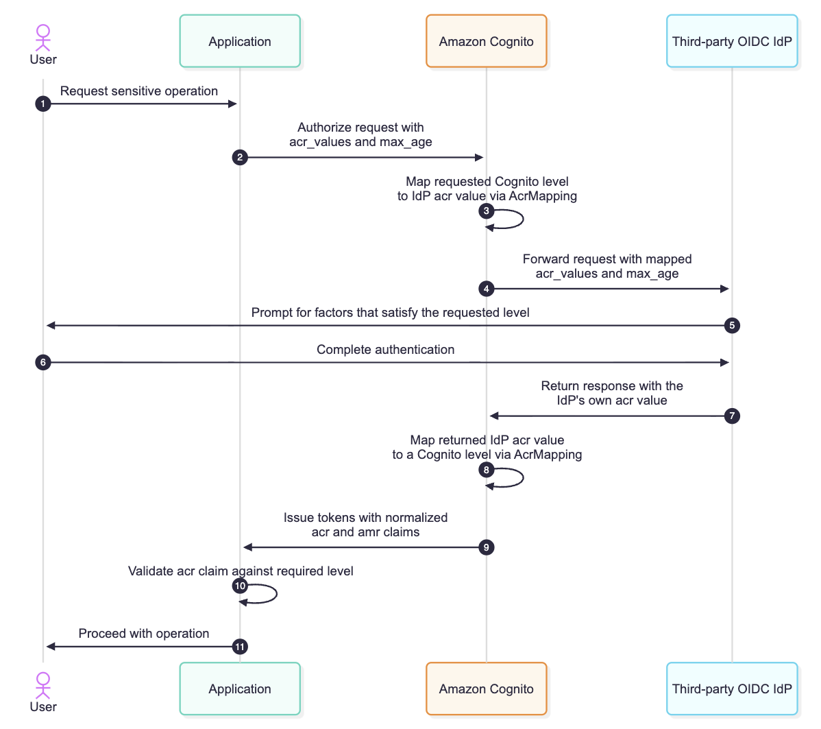
The interaction gains a third participant, the downstream IdP, but the assurance requirement is persisted through the entire federated authentication flow as shown in figure 2.
Figure 2: Federation with an OIDC third-party IdP, persisting the acr_values and max_age request parameters
The value that comes back from a partner IdP won’t use Amazon Cognito’s level URIs, so this lets you map the provider’s acr values onto its own levels with the AcrMapping field on the OIDC IdP configuration. A partner IdP that reports, say, https://partner.example/assurance/strong can be mapped to Amazon Cognito level 3 (urn:cognito:loa:3), so that by the time the token reaches your application the acr claim speaks the same vocabulary regardless of whether the user authenticated locally or through a federated provider. Your resource server keeps a single enforcement rule and authorization logic and doesn’t need to have special handling depending on where the user ultimately authenticated. See Step-up authentication for federated users to learn how to map external OIDC IdP acr levels to Cognito.
This is the same pattern that RFC 9470, the OAuth 2.0 Step Up Authentication Challenge Protocol, describes: the assurance level is requested at the edge of your application, travels through Amazon Cognito to whatever provider authenticates the user, and returns normalized to a vocabulary your code already understands. A user federating from a corporate IdP and a user signing in against the same user pool directly both arrive at your resource server carrying an acr claim that means the same thing.
Conclusion
In this post, I showed you how the acr and amr claims in Amazon Cognito let you match authentication strength to the risk of what a user is doing, instead of settling for one bar at the front door. Your application requests a target level with acr_values and max_age (or TARGET_ACR_VALUES and MAX_AGE in the USER_AUTH flow), Amazon Cognito reports the level reached and the methods used, and your application enforces what each operation requires. The four patterns, from a banking transfer to a federated third-party IdP, follow that same loop, and one enforcement rule at your resource server covers every sign-in path.
The larger shift is that assurance is now something Amazon Cognito expresses in a standard way and your application reasons about directly, without building your own step-up tracking. To get started, move your user pool to the Essentials or Plus feature plan, decide the level each operation requires, and add acr_values to your existing authorize requests. For the complete parameter reference and federated behavior, see the Amazon Cognito Developer Guide.
If you have questions about this post, contact AWS Support or start a new thread on AWS re:Post.
Building long-term observability for Amazon Redshift starts with a question: what happened in your data warehouse last month, last quarter, or last year? Amazon Redshift captures operational history across more than 25 system views. These views range from query execution details in SYS_QUERY_HISTORY and full query text in SYS_QUERY_TEXT to connection activity, user changes, workload management events, and resource consumption metrics. Together, these views form a detailed record of the operations running inside your Amazon Redshift clusters and Amazon Redshift serverless workgroups. Amazon Redshift retains this data for 7 days. After that window closes, the history is gone. You lose the ability to audit past activity, investigate slow-moving regressions, or satisfy compliance requirements that can span months or years.
The system table integration with Amazon S3 Tables, a capability of Amazon Redshift, changes this. When you enable the integration, Amazon Redshift automatically and continuously delivers system table data as Apache Iceberg tables to Amazon S3 Tables in your account. You own the data, you set the retention policy, and S3 Tables handles compaction and snapshot maintenance. You can query the exported data with Amazon Redshift, Amazon Athena, or any Iceberg-compatible engine. There’s no charge for delivery. You pay only for S3 Tables storage, requests, maintenance, and the engine you use to read the data.
AWS and Datadog collaborated to make this exported data actionable for observability. Datadog, an AWS Specialization Partner and AWS Marketplace Seller, provides an observability and security platform for cloud applications. Datadog Data Observability helps data teams improve the reliability of data for analytics and AI. It combines quality monitoring for warehouses such as Amazon Redshift with jobs monitoring for pipelines that run on AWS Glue, Amazon EMR, Apache Airflow, and dbt. It then connects them with lineage that spans from source pipelines to downstream dashboards. By reading query history directly from S3 Tables, Datadog turns it into column-level lineage, query analysis, and context for quality alerts, without adding load to your warehouses to collect it. For AWS managed monitoring of Amazon Redshift metrics and logs, you can also use Amazon CloudWatch. Datadog Data Observability is billed separately by Datadog.
In this post, we show how to configure Datadog Data Observability to read Amazon Redshift query history from S3 Tables. We walk through granting Datadog read access and using the query history for column-level lineage, query analysis, and data quality monitoring.
Solution overview
Datadog Data Observability uses Amazon Redshift query history to build column-level lineage, analyze query performance, and give context to data quality alerts. Previously, Datadog collected this history by running read-only SQL against each warehouse every hour. With this solution, Datadog reads the same history from S3 Tables instead. The following diagrams show the solution at a high level and compare query history collection before and after the integration.
Figure 1: High-level solution overview
Figure 2: Query history collection before and after the S3 Tables integration
This approach offers the following benefits:
Retention beyond 7 days. Query history remains in your account for as long as you choose to retain it. Because history is kept in S3 rather than expiring after 7 days in the cluster, Datadog can backfill any collection gap when it resumes. You don’t lose queries or lineage. Your audit and compliance teams also keep a long-term record of query activity in your own account.
No added load on the warehouse. Datadog reads the Iceberg tables through the S3 Tables Iceberg REST endpoint. Collecting query history doesn’t run queries on your clusters or workgroups or consume their compute.
One view across warehouses. Datadog combines query history from every connected cluster and workgroup into a single lineage graph, together with other connected tools such as dbt, Apache Airflow, Tableau, Looker, and Power BI.
The following diagram illustrates the solution architecture.
Figure 3: Solution architecture
The workflow consists of the following steps:
Amazon Redshift periodically writes completed query records from SYS_QUERY_HISTORY and SYS_QUERY_TEXT to the AWS managed aws-redshift table bucket in Amazon S3 Tables. An isolated background process handles these writes, separate from your production workloads.
Datadog uses the AWS Identity and Access Management (IAM) role from your Datadog AWS integration to read new rows through the S3 Tables Iceberg REST endpoint. Because data is delivered in batches at a fixed frequency, Datadog tracks the last batch it read, so no batch is skipped or read twice.
Datadog masks sensitive literals in the query text, parses each query into column-level lineage, and groups similar queries into normalized query profiles.
Datadog still connects to Amazon Redshift for table metadata, such as schemas and row counts, and to run the data quality monitors that you configure.
Prerequisites
To implement this solution, you need the following:
An AWS account with one or more Amazon Redshift provisioned clusters (RG or RA3 node types) or Amazon Redshift Serverless Workgroup.
The system table integration with Amazon S3 Tables enabled for each warehouse you want to monitor. At minimum, enable sys_query_history and sys_query_text. Datadog reads per-warehouse exports, so set the granularity to cluster for provisioned clusters or workgroup for Serverless namespaces. To enable the integration, see Enabling system table integration with Amazon S3 Tables.
The Amazon S3 Tables integration with the AWS Glue Data Catalog enabled in your account and Region. This is a one-time setup step. If you already integrated S3 Tables with the AWS Glue Data Catalog, no further action is needed. For instructions, see Integrating Amazon S3 Tables with AWS analytics services.
An IAM principal with the following permissions:
redshift:EnableLogging (provisioned) or redshift-serverless:UpdateNamespace (Serverless).
s3tables:CreateTableBucket, s3tables:PutTableBucketEncryption, and s3tables:PutTableBucketPolicy.
A Datadog account with the Datadog AWS integration configured and your warehouse connected to Datadog Data Observability for Amazon Redshift.
Access to the Datadog Data Observability S3 Tables preview. To request access, contact your Datadog account team.
Note: Plan your encryption strategy before enabling the integration. If you encrypt the tables with a customer managed AWS Key Management Service (AWS KMS) key, you can’t change the key after the tables are created. If you plan to consolidate warehouses later, choose a shared AWS KMS key from the start.
Grant Datadog read access to the system tables
Datadog reads the system tables with the IAM role that your Datadog AWS integration uses. Complete the following steps:
On the IAM console, in the navigation pane, choose Roles, then choose the role used by your Datadog AWS integration.
Choose Add permissions, then choose Create inline policy.
Choose the JSON tab and enter the following policy, replacing <region> and <account-id> with your values:
Enter a name for the policy, for example DatadogRedshiftSystemTablesRead, and choose Create policy.
Note: If you encrypted the tables with a customer managed AWS KMS key, also grant the role kms:Decrypt permission on that key.
Use S3 Tables as the query history source in Datadog
During the preview, your Datadog account team enables S3 Tables as the query history source for your Datadog organization. Datadog then reads query history for each connected Amazon Redshift warehouse from S3 Tables instead of from the warehouse. Datadog tracks its position in the query history for each warehouse, so switching between sources doesn’t skip or duplicate queries.
Analyze query history in Datadog Data Observability
Query history feeds three parts of Datadog Data Observability:
Lineage. Shows how data moves between tables, jobs, and dashboards.
Query analysis. Shows who produces and consumes that data, and at what cost.
Quality monitoring. Uses both to decide which tables to watch and to explain each alert.
Datadog builds all three from the same query history, so they work the same way whether the history comes from the warehouse or from S3 Tables.
The examples in this section use an Amazon Redshift table named analytics.fct_orders. A nightly job loads it from staging.stg_orders, and a Tableau dashboard reports revenue from it.
Note: The figures use a sample environment, so they show a database named prod and a table named int_orders_enriched instead of analytics.fct_orders.
Column-level lineage
Figure 4: End-to-end lineage upstream of, through, and downstream of the prod database
Datadog parses each query in the history into column-level lineage. To explore it, complete the following steps:
Choose Data Observability, then Lineage.
Search for prod to anchor the graph on the database. Figure 4 shows the result: source tables such as orders flow through the raw, staging, and intermediate schemas into marts. To focus on a single table such as users, search for that table instead.
Review upstream tables and jobs to the left, and downstream tables and dashboards to the right. An Upstream issue label marks assets affected by a problem further upstream.
To see column-level lineage, expand a table to show its columns and how each one flows into downstream tables. To trace a single column from source to dashboard, change the asset type to Column and search for it.
In addition to Amazon Redshift, the lineage graph supports other sources. When you connect other integrations, upstream jobs from Apache Airflow or dbt and downstream dashboards from Tableau, Looker, or Power BI appear in the same graph. Datadog builds lineage from the query history in the time window you choose, so widen the window to include jobs that run weekly or monthly.
Two common lineage workflows are:
Root cause analysis. Anchor on a broken table or dashboard, set the downstream depth to 0, and step upstream. Tables flagged by a quality monitor show their status on the graph, so you can see where a problem starts.
Impact analysis. Before you change or drop a column, anchor on it, set the downstream depth to the maximum, and switch to the List view to see every table and dashboard that depends on it.
Query analysis
Query analysis turns your Amazon Redshift query history into trends, so you can catch queries that slow down or scan more data over weeks and months, not just the last 7 days. Figure 5 shows the result for the last question: an INSERT run by the etl_svc user.
Figure 5: Query count, execution time, and data scanned for a normalized INSERT pattern
To explore query patterns:
Choose Data Observability, then Queries, and choose Amazon Redshift.
Review normalized query patterns. For each pattern, Datadog shows how often it runs, how long it takes, and how much data it scans.
Group patterns by query, cluster, user, database, or statement type.
Filter by the tables they read or write.
Because Datadog combines the query history from every connected cluster and workgroup, you can answer the following questions across your whole Amazon Redshift footprint:
Which query patterns take the longest or read the most data?
Which users or service accounts run the most expensive queries?
Which queries write to analytics.int_orders_enriched, and how has their runtime changed over time?
Quality monitoring
Quality monitors alert you when an Amazon Redshift table is not updated, changes unexpectedly in volume, or contains values that fall outside its normal range. Lineage then shows the upstream cause and the downstream impact.
Figure 6: An anomaly monitor on orders per hour in Datadog
Data Observability monitors track the following metrics:
Freshness
Row count
Column-level metrics such as nullness and uniqueness
Custom SQL metrics
Each monitor can use anomaly detection, which learns a metric’s trends and seasonality so that you don’t need to set a threshold for every table. Figure 6 shows an anomaly monitor on orders per hour, grouped by traffic source. When the metric falls outside its expected range, Datadog flags the likely upstream cause and the downstream assets at risk. Schema change monitors (currently in preview) alert when an Amazon Redshift table or column is added, removed, or renamed, or when a column type changes.
Lineage also helps you decide what to monitor. For example, add a relation filter to monitor every table upstream of a specific dashboard.
Quality monitoring runs aggregate queries in Amazon Redshift, such as COUNT(*) and MAX(<timestamp_column>), and sends only the resulting values to Datadog, not rows from your tables. To protect sensitive columns, you can use Amazon Redshift dynamic data masking.
Example: Trace a stale dashboard to its cause
The following steps show how these features work together when the revenue dashboard stops updating:
A freshness monitor on analytics.fct_orders alerts in Slack that the table hasn’t updated since its usual 02:00 load.
On the Lineage page, you anchor on fct_orders. The monitor on the upstream table staging.stg_orders is healthy, so the source data arrived and the problem is in the step that builds fct_orders. The graph also shows that the Tableau revenue dashboard depends on fct_orders.
On the Queries page, you filter to queries that write to analytics.fct_orders. The nightly INSERT pattern run by the etl_svc user shows failed runs starting at 02:00.
You fix the job and, before you rerun it, use impact analysis to list the downstream tables and dashboards whose owners you notify.
Clean up
To stop writing system table data to S3 Tables, for a provisioned cluster, run the following command:
Before you run the preceding commands, ask your Datadog account team to switch the query history source back to the warehouse. Datadog then resumes collecting query history from your warehouse where it left off, so lineage and query analysis continue without a gap.
Disabling the integration stops new deliveries but keeps the data that was already written. Amazon Redshift doesn’t deliver system table data to S3 Tables while the integration is disabled, so your long-term record in S3 Tables won’t include that period. Re-enabling the integration doesn’t backfill that period, and after 7 days, Amazon Redshift no longer retains those queries in the warehouse either. To stop incurring storage charges, delete the tables. Deleting the tables permanently removes the retained data, and Amazon Redshift doesn’t recreate them automatically.
Conclusion
In this post, we showed how to configure Datadog Data Observability to read Amazon Redshift query history from Amazon S3 Tables. With this integration, you can:
Retain query history beyond the 7-day in-cluster limit for auditing and compliance.
Collect query history without adding load to your warehouses.
Analyze lineage and query activity across all your clusters and workgroups in one place.
AWS and Datadog built this integration together so you can use Amazon Redshift system table data in your existing observability workflows.
If you’re new to Datadog, you can sign up for a free trial. If you have questions or suggestions, leave them in the comments.
Most organizations run a multicloud estate, and so do the attackers targeting them. An adversary who compromises an identity in one provider follows that identity wherever it leads, including across a federated trust into a second cloud service provider. The signals enumerating this scenario are rarely missing; the problem is that they live in separate consoles, in different schemas, owned by different teams. No one has visibility into the whole picture, so no one can decide what to fix first.
AWS Security Hub addresses prioritization and triage with exposure findings. Security Hub correlates reachability, blast radius, vulnerabilities, misconfigurations, and effective permissions, providing a strong correlation layer with an attack-path visualization, providing the context needed to generate risks from findings. That analysis now extends to Microsoft Azure. Security Hub records and analyzes your Azure resources with the same correlation engine used for Amazon Web Services (AWS) resources. The resulting details and meta-data land in the same console, ranked in the same queue, providing holistic, multicloud visibility into your security risks.
In this blog post, you learn how to configure the Azure integration for Security Hub and use exposure findings to prioritize attack paths across both clouds from one console. We follow a realistic scenario: a compromised identity that threatens both an Azure and an AWS environment through a shared, federated identity plane. We show you how the critical exposures along that path are presented as ranked findings that you can triage together, and we map each one to the MITRE ATT&CK framework. We also cover the prerequisites that teams commonly overlook.
Why prioritizing multicloud risk is difficult
Consider an organization whose Microsoft Entra ID tenant is federated into an AWS account, so identities in the tenant can assume an AWS role. This is an ordinary and intentional configuration used to avoid having to manage a second set of credentials. It also means the two clouds share an identity plane: a single compromised Entra identity is both an Azure threat and—through the federation—an AWS threat.
An attacker exploits this, but the defensive signals land in different places:
Each team sees one fragment, and in isolation each fragment appears low severity. You see the risk only when you correlate all of it together and discover the same identity plane ties the attack path together. Exposure findings provide that severity within AWS; extending it to Azure closes the multicloud visibility gap.
How the Azure integration works
You create the Azure connector in the AWS Management Console for Security Hub. It authenticates to your Entra ID tenant through an application registration, records and evaluates your Azure resource configurations, and streams Microsoft Defender for Cloud alerts and Entra ID audit logs through an Azure Event Hubs namespace. Your Azure resources then flow into the same correlation engine that analyzes signals from AWS Security Hub Cloud Security Posture Management (CSPM), Amazon Inspector, Amazon Macie, and Amazon GuardDuty. That engine produces two kinds of findings:
Control findings against standards such as the CIS Microsoft Azure Foundations Benchmark.
Exposure findings, which are ranked, attack-path findings that correlate traits such as reachability, effective permissions, and misconfiguration, with a severity based on how discoverable and exploitable the risk is.
Both use the Open Cybersecurity Schema Framework (OCSF) and appear in the same console as your AWS findings. However, one filtering detail matters: because Security Hub produces the finding, its top-level cloud.provider is AWS, while the evaluated resource carries resources[].provider = Azure. Filter on resources.provider to scope to a single cloud.
Prerequisites
To follow along with this post, you need:
An AWS account with Security Hub enabled. If you use a delegated administrator account for Security Hub, create the connector there, in the AWS Region where you aggregate findings.
An Entra ID tenant with a Microsoft Azure subscription. You need privileges in Azure to create an application registration, assign roles at the tenant root management group, and create a subscription-level diagnostic setting.
The Azure CLI, authenticated to the target subscription with az login command.
Activity log export. Azure resource recordings are change-driven and depend on activity logs reaching the event hub that the connector reads. The onboarding process assigns an Azure policy to create the required diagnostic setting, but it only remediates existing subscriptions after you create a remediation task. If the connector reports healthy status but resources never appear, run az monitor diagnostic-settings subscription list to confirm the export exists, and create a remediation task if the list is empty.
Configuration
The following steps detail how to connect your Azure environment to Security Hub v2: Registering the Azure application, establishing federated identity credentials, and assigning the roles required for AWS to evaluate your Azure resources.
Step 1: Create the Azure connector in Security Hub
The first step in this configuration is to create the Azure connector in Security Hub. The connector establishes trust with your Azure tenant and defines which subscriptions and regions Security Hub v2 will evaluate.
Open the Security Hub console and choose Integrations.
Choose Create Azure connector.
Enter your Azure Tenant ID and the Application (client) ID of the application registration you created for the integration.
For Subscriptions and Regions, select all. Attack paths cross subscription and Region boundaries, so partial coverage leaves blind spots where a compromised identity can pivot unseen. Scope to specific IDs or Regions only when data-residency rules require it.
Run the generated setup script in your Azure environment, then choose Create connector.
Include the global region scope. Controls that evaluate Entra ID and Microsoft Graph resources require it, and those identity exposures are central to this scenario. If you also create an Amazon Inspector or Security Hub CSPM connector for the same tenant, keep its subscriptions and regions consistent with this one.
Step 2: Verify the connector and its recording activity
Health status alone doesn’t tell you whether recording is flowing. Confirm both.
Step 4 (optional): Add Amazon Inspector for Azure vulnerability scanning
To add vulnerability findings for Azure virtual machines (VMs), function apps, or container registry images, create an Amazon Inspector connector for the same tenant. VM scanning requires each target VM to have a system-assigned managed identity, which you can enforce with an Azure Policy. Figure 1 shows a correctly configured Azure integration inside Security Hub, with vulnerability management and posture management deployed.
Figure 1: Successful configuration of the Azure integration with Security Hub
Walk-through: Prioritizing a cross-cloud attack path
In this example, the organization has one identity plane across two clouds, comprising a Microsoft Entra ID tenant with a federated trust into an AWS account. An adversary who compromises the right Entra identity gains an initial foothold in Azure and a path into AWS, because both clouds trust the same identity plane. The following sections trace that path. Each step is a real, high-severity exposure finding that Security Hub ranked on its own. The point of the walk-through is to demonstrate a real-life scenario and examine all findings in one unified security console.
The path begins with an Entra identity that is both over-privileged and unprotected. You’ll find this in the Security Hub console under Exposures, where Security Hub raises it as an identity exposure finding and maps the attack path stemming from it:
Potential Unauthorized Access: Azure RBAC user with administrative access has MFA disabled (high). It correlates the user, the role assignment that grants administrative access, and the organization.
The tenant’s authorization policies let an attacker broaden that foothold, and Security Hub CSPM reports each policy as a failed control (high): Microsoft Entra ID authorization policies should prohibit default users from registering applications…should restrict user consent for applications, and Azure authorization policies should restrict guest invitations to admin roles only. Each finding expands what a single compromised, non-privileged identity can do without an administrator.
Phase 2: Foothold and privilege escalation (Azure)
The tenant contains an internet-reachable VM whose network security group allows inbound from any address, and whose attached identity holds administrative rights over the subscription. Security Hub surfaces this under Exposures, correlating reachability and effective permissions into one finding that shows why it matters: anyone reaching the VM inherits admin control of the subscription.:
Potential Initial Access: Potentially internet reachable Azure virtual machine with open network security group has administrative access (high). It correlates the VM, the role assignment, the network security group, and the public IP address.
The finding’s analysis reads like an attack path. The resource “may be reachable from the public internet,” “overly permissive network security group (NSG) rules allow unintended inbound access,” and “the Owner or Contributor role grants extensive permissions… enabling a threat actor to escalate privileges.” Security Hub evaluates this from configuration and network-path modeling, so it surfaces whether or not the VM is running. Figure 2 shows the correlated attack path for that virtual machine.
Figure 2: An Azure attack-path exposure, analyzed by the same correlation engine as AWS exposures
The cross-cloud bridge: Federation into AWS
The tenant from Phases 1 and 2 is federated into the AWS account through an IAM SAML identity provider. As shown in Figure 2, a role trusts that provider and grants read access to every bucket in Amazon Simple Storage Service (Amazon S3). This trust is what expands the risk across clouds from the same adversary: a compromised Entra identity can assume this role and reach AWS data.
This one hop lives in IAM rather than in Security Hub. Security Hub doesn’t not raise a finding for a role that trusts your own federated identity provider. Confirming it is a normal investigative pivot: the role trusts a SAML identity provider that represents your Entra tenant, the same tenant whose exposures you triaged when you added Amazon Inspector in Step 4.
Figure 3: The federated trust that links the two clouds through a shared identity plane
Phase 3: The impact (AWS)
ATT&CK: Data from Cloud Storage (T1530), Transfer Data to Cloud Account (T1537)
On the AWS side, the correlation engine has already categorized the resources this identity can reach. Under Exposures in the Security Hub console, the sensitive-data objective surfaces this finding because that reachable set includes data at risk; a compromised identity could destroy it:
Potential Sensitive Data Destruction: S3 bucket has sensitive data and versioning disabled and Object Lock disabled and MFA delete disabled (high). A Macie finding, The S3 object contains personal information, is a contributing signal, and the control S3 general purpose buckets should be encrypted at rest with AWS KMS keys fails alongside it.
The same account carries related AWS attack-path exposures. Two examples are Potential Resource Hijacking: Internet reachable EC2 instance with open security group has software vulnerabilities with limited effective permissions and Potential Unauthorized Access: IAM user has weak password policies. In the exposure queue, these sit next to the Azure findings, ranked by the same severity model.
Prioritizing across both clouds in the console
Here is the operational benefit. An analyst is notified of generated exposure findings and opens the dashboard and filters to High severity. In one prioritized list, without switching tools or opening a ticket for another team, they see the Azure admin identity without MFA, the internet-reachable Azure VM with subscription-admin rights, and the AWS sensitive data exposure. Together, these show the full scope of what a single vector, sharing an identity plane, might target. The analyst confirms the connecting federation with one pivot into IAM. The multicloud triage that used to require two products and two teams now occurs in one place. Figure 4 shows that single ranked queue.
Figure 4: Cross-cloud exposure prioritization in a single console
Phase-to-exposure summary
The following table traces each phase of the attack path to its MITRE ATT&CK techniques, the cloud where it plays out, and the ranked Security Hub exposure that surfaces it — following the pivot from Azure into AWS across the shared identity plane.
Phase
ATT&CK
Cloud
Ranked exposure in Security Hub
1. Compromised identity
T1566, T1078.004
Azure
Potential Unauthorized Access: Azure RBAC user with administrative access has MFA disabled (High)
2. Foothold and privilege escalation
T1190, T1078.004
Azure
Potential Initial Access: internet reachable Azure VM with open NSG has administrative access (High)
2.1 Bridge
T1550 (Use Alternate Authentication Material)
Azure to AWS
Federated trust, confirmed in AWS IAM (shared identity plane)
3. Data objective
T1530, T1537
AWS
Potential Sensitive Data Destruction: S3 bucket has sensitive data… (High), plus Macie
Conclusion
A cross-cloud attack is difficult to prioritize because signals are generated across separate consoles, schemas, and teams. In this post, you saw how the Azure integration for AWS Security Hub brings Azure resources into the same exposure engine and the same queue as your AWS resources. One analyst can prioritize an attack path that spans a compromised Microsoft Entra ID identity, across a federated trust, to sensitive data in Amazon S3, without leaving Security Hub.
To recap why this workflow is practical and effective:
Security Hub records and analyzes your Azure security findings and displays them in the same unified console as your AWS resources, and produces ranked, attack-path exposure findings for both clouds.
Findings from both clouds share the OCSF schema, so you filter, group, and prioritize them in one place. Filter on resources.provider to scope an individual cloud.
Security Hub correlates signals into attack paths within each cloud. The analysis creates a cross-cloud narrative, such as a shared federated identity plane, while co-locating ranked correlation findings across both Azure and AWS, creating efficient scoping and remediations.
Confirm your prerequisites. Include the global region scope for Entra ID controls, know that sign-in log signals require an Entra ID P1 or P2 license, and confirm that the subscription diagnostic setting that exports Activity Logs to the connector’s event hub is in place. A connector can report a healthy status while it records nothing.
Cloudflare has become a neolab. We’re building our own frontier AI models for our customers and the open-source community.
Today, we’re announcing two open-weight model releases:
We’re introducing an updated version of Clairic. Since the preview, we’ve improved extraction from complex documents including images and PDFs (new!), with more reliable handling of tables, lists, and dates, and better grounding of answers in the source material.
We’re introducing Clairic-flash, a lighter, faster version of Clairic that delivers strong extraction and prediction performance in a compact, 9-billion-parameter model.
Both extraction models are hosted on Workers AI and full open weights are available on Hugging Face.
We’re also excited to re-introduce ourselves as the Workers AI superintelligence team, the frontier AI research team behind Clef, Clairic, and lots more in the works. This team is working quickly to push the AI frontier and build useful models for Cloudflare’s customers and the open source community.
A new version of Clairic: redesigned after the preview release
Since announcing Clairic in preview, we have received a ton of use cases and helpful feedback on how customers wanted to use an extraction model. We heard about use cases ranging from extracting data from images like receipts to reading values from support tickets. We knew that we wanted extraction to be the clear focus for the model, so it had to excel at reading from unstructured data.
We decided to go back to the drawing board with Clairic and redesigned our architecture, differentiating this new version of Clairic from our preview release. For ordinary text and number extraction fields, we now use parallel slot autoregressive generation instead of a single forward pass. Each field uses the tokens it has already written to choose its next token, then stops at its own end marker. All the fields advance together in the serving batch, still giving lightning-fast latency per request. This boosted our accuracy in extraction for both text and images, and the trade-off in accuracy offsets the small latency cost. For computation, estimation, and extraction use cases, we trained special heads that can handle estimates, forecasts, durations, calculated dates, and explicit arithmetic.
Although the model architecture evolved, we kept the parts of the typed API interface that make the answers useful: confidence scores, character spans, and probabilities are still intact with every request. The model is still incredibly fast and cheap. From the evals below, you can see how our newer versions of Clairic have greatly improved on extraction across text, images, PDFs, and more.
There are no public extraction benchmarks yet, but we ran our internal evals for other emerging extraction models on the market, such as Liquid AI’s D1.2 (pipelined with Apple Vision for optical character recognition) and Scaledown’s Extract. Our Clairic models excel across extraction use cases, but take these evals as directional guidance since they are self-reported. We wanted to show an illustrative picture of how Clairic is performing across generalized extraction use cases and celebrate the fact that other companies are releasing extraction models as well — confirming our original hypothesis that extraction was a pain point for LLM users because of the cost, latency, and accuracy.
But is it fast?
We ran latency tests for Clairic and Clairic-flash, measuring complete HTTP response from a self-hosted server, including all fields in the request. Even with the redesigned architecture, you can expect responses in under one second — much faster than typical LLM responses for similar workloads.
Eval set
Requests per model
Clairic p50 / p95
Clairic-flash p50 / p95
Fresh text fields
96
358 / 736 ms
155 / 328 ms
Fresh image fields
48
453 / 976 ms
305 / 605 ms
Commercial leases
180
691 / 803 ms
379 / 519 ms
Loan pricing
600
395 / 407 ms
188 / 192 ms
Traffic forecasting
114
532 / 585 ms
243 / 261 ms
Expense audit, development
60
632 / 742 ms
393 / 512 ms
Better extraction for images and PDFs
In our preview blog post, Clairic read a photo of a receipt. Now the Clairic family of models can read PDFs too, so you can ask for the supplier, line items, and total in one request, even when they appear on different pages. You can include up to four images or PDF pages in total, and line items can come back as rows that keep each description, quantity, and price together. Due to Clairic’s new architecture, image reading accuracy has improved from 207 errors to 0 on our internal benchmarks, explicitly covering text and images.
Promotional pricing on Clairic for a limited time
When we first launched our preview endpoint of Clairic at @cf/cloudflare/clairic, we hosted the 9B variant as it was faster and easier to train, at the preview price of $0.10 per M input tokens. We’re now moving the 9B model to the @cf/cloudflare/clairic-flash endpoint and the 27B model will live at @cf/cloudflare/clairic.
The 27B Clairic model will be priced at $0.24 per M input tokens, while the 9B Clairic-flash model will be priced at $0.10 per M input tokens. Although the model does technically generate output tokens, we decided to keep the System One pricing principles and are only charging on input tokens: we eat the cost of the output token generation.
In order to make this a seamless swap, we’re offering a promotional discount on Clairic — until December 1, 2026, both Clairic and Clairic-flash will cost $0.10 per M input tokens. This means you get to try out the higher quality variant of Clairic at the same price. If your applications are hooked up to the Clairic endpoint that we released in preview, you will automatically benefit from the better extraction capabilities of our new model, which we’re rolling out in place.
If you’d like to move more cost-sensitive workloads to the cheaper 9B Clairic-flash variant, we encourage you to do so. On December 1, we’ll be ending the promotional discount for Clairic and pricing will resume at $0.24 per M input tokens instead of the discounted $0.10 per M input tokens.
Clairic and Clairic-flash (new) are open-weight
Both Clairic models are now open-weight on Hugging Face as well. We have seen an outpouring of experiments and tuned models from our release of Clef, and we’re happy to continue supporting teams and research with our open-weight release of Clairic.
Our mission with these System One models is to help people augment their expensive LLM usage with smaller, faster, cheaper models that are purpose-built for a specific task. We hope that releasing these models open-weight encourages others to experiment and build on our ideas as well.
Try them out
Clairic and Clairic-flash are available on Workers AI as @cf/cloudflare/clairic and @cf/cloudflare/clairic-flash. The developer documentation has the full API schemas, which remain unchanged from our preview endpoint. We’re also publishing the open-weight releases for Clairic and Clairic-flash on Hugging Face.
The team behind these models — the Workers AI superintelligence team — is just getting started, and growing fast to push frontier AI research at Cloudflare. Join us early and help shape what the superintelligence team becomes.
Apache Airflow orchestrates data pipelines ranging from data ingestion and machine learning to SQL-based analytics. Some analytical workloads, such as daily rollups and usage reports, process bounded datasets and can run within the resources of a single worker. For these workloads, deploying a distributed query cluster can add unnecessary infrastructure and operational complexity.
DuckDB is an open source in-process analytical database that runs within an application without requiring a separate database server. Its columnar, vectorized execution engine supports analytical SQL operations, including scans, joins, and aggregations.
Amazon Managed Workflows for Apache Airflow (Amazon MWAA) runs Apache Airflow as a managed service, so you can schedule, run, and monitor workflows without managing the underlying Airflow infrastructure. Combined with DuckDB, you can add SQL transformations to your pipelines that run inside the Airflow task itself.
In this post, you learn how to run DuckDB with an Amazon MWAA Provisioned environment.
How DuckDB and Amazon MWAA work together
In Apache Airflow, a directed acyclic graph (DAG) defines tasks and their dependencies, along with scheduling, retry, and concurrency settings. Amazon MWAA runs the tasks on workers and publishes configured task logs to Amazon CloudWatch Logs.
DuckDB runs in the Airflow task process, using the CPU, memory, and local storage of the Amazon MWAA worker container. Amazon MWAA orchestrates the workflow, while DuckDB performs the SQL processing.
This walkthrough uses DuckDB 2.0.0, which includes asynchronous I/O for reading from object storage and first-class VARIANT support for semi-structured data. DuckDB 2.0.0 also supports a client-server mode through the Quack protocol, which lets other processes connect to a DuckDB database over the network. This walkthrough runs DuckDB in-process because each Airflow task performs a self-contained transformation.
Introducing the Apache Airflow DuckDB provider
The Apache Airflow DuckDB provider provides the DuckDBExecuteQueryOperator. The operator runs DuckDB locally in the worker container and executes SQL without starting a separate query service.
The DuckDB integration in the Amazon provider adds the AWS aware duckdb_aws connection type. On supported Amazon MWAA Provisioned environments, the DuckDB packages are preinstalled, and Amazon MWAA creates the default connection, as described later in this post.
Solution overview
An engineering team operates a shared inference service that product teams use for their applications. As usage grows, the team needs to understand which applications and teams are driving inference activity and the estimated cost of that usage. Showback provides an itemized view of usage and estimated cost without charging teams directly.
To build the showback pipeline without a separate analytics cluster, the team uses Amazon MWAA to orchestrate Airflow tasks that run DuckDB. DuckDB reads source files from Amazon Simple Storage Service (Amazon S3), performs SQL transformations, and publishes the results as Apache Iceberg tables in Amazon S3 Tables. This pattern suits bounded, SQL-oriented workloads that run reliably within the resources of a single worker.
Figure 1: Amazon MWAA orchestrates two DuckDB tasks across five stages, from reading Parquet data in Amazon S3 through publishing and validating Iceberg tables in Amazon S3 Tables
The workflow has five logical stages, implemented by two Airflow tasks, as shown in Figure 1.
Stage 1: Store the source data – An Amazon S3 bucket stores the Parquet files for inference events, model rates, and application ownership records.
Stage 2: Trigger the DAG – A manual action starts this example DAG. Amazon MWAA orchestrates both tasks, tracks their status, and sends task logs to Amazon CloudWatch Logs. You can configure a schedule for recurring runs.
Stage 3: Read, clean, and combine the records – The transform_and_publish_showback task uses DuckDB to read the Parquet files directly from Amazon S3, deduplicate events, and apply the model rate and ownership record effective at each invocation timestamp.
Stage 4: Publish the result – In the same transform_and_publish_showback task, DuckDB merges the processed records into the costed_invocations Iceberg table in Amazon S3 Tables and commits the update. The task also creates the daily_application_showback and team_budget_status summary tables.
Stage 5: Validate published tables – After publication, the second Airflow task, validate_showback, uses DuckDB to check the row count, confirm that event IDs are unique, and verify the expected allocation states.
The sample rates and cost_credits values are synthetic and are provided only to demonstrate allocation logic. They do not represent AWS pricing, Amazon Bedrock charges, or customer billing records.
Prerequisites
Before you begin, make sure you have the following resources and permissions:
An Amazon MWAA Provisioned environment running Apache Airflow 3.3.1 with Python 3.12. See Apache Airflow versions on Amazon MWAA for the currently supported versions.
An Amazon S3 bucket for the source Parquet files and an Amazon S3 Tables table bucket for the outputs.
An Amazon MWAA execution role with read access to the source bucket and permissions to create, read, and update tables and table data in the target table bucket. For the required actions, see Accessing Amazon S3 Tables using open source applications. If the table bucket uses a customer managed AWS Key Management Service (AWS KMS) key, the role also needs permission to use that key.
Network connectivity from the Amazon MWAA private subnets to Amazon S3 and Amazon S3 Tables. This sample installs the DuckDB Iceberg extension at runtime, so it also requires access to the official DuckDB extension repository unless the matching extension is already available.
The sample bundle containing the DAG, SQL, and synthetic-data generator used in this walkthrough.
Python 3, the dependencies listed in generator-requirements.txt, and the AWS Command Line Interface (AWS CLI) configured on the workstation where you generate and upload the sample data.
In the test environment used for this post, Amazon MWAA included apache-airflow-providers-amazon 9.38.0, apache-airflow-providers-duckdb 0.2.0, and DuckDB 2.0.0. These versions might change in future Amazon MWAA releases.
Use the built-in DuckDB providers and connection
Amazon MWAA Provisioned environments running Apache Airflow 3.3.1 include DuckDB, the Apache Airflow DuckDB provider, and the DuckDB integration in the Amazon provider. Amazon MWAA also creates a connection named duckdb_default with the connection type duckdb_aws. You do not need to add packages to requirements.txt or create the connection manually.
To confirm that the connection exists, choose Admin, then Connections in the Airflow UI. Look for duckdb_default.
Note: When a DuckDBExecuteQueryOperator task doesn’t specify conn_id, it uses duckdb_default. The AWS aware hook obtains temporary credentials from the Amazon MWAA execution role and creates a DuckDB S3 secret for the task. Don’t put AWS access keys in the DAG or create a separate S3 secret in the SQL, because doing so can conflict with the secret the hook creates. If duckdb_default doesn’t appear under Admin, Connections, update your Amazon MWAA environment without changing any settings to apply the latest Amazon MWAA image.
Prepare the sample data
Use generate_ai_inference_data.py from the sample bundle to create Parquet files containing inference events, model rates, and application ownership records. A fixed random seed makes the input reproducible. The dataset includes duplicate events and changes to rates and ownership, allowing you to demonstrate deduplication and effective-dated attribution.
Run the generator and upload the resulting files to Amazon S3:
The default settings generate approximately 300,000 unique events across daily partitions. The generated manifest.json records the expected unique-event count for subsequent validation.
Build the DuckDB transformation
See publish_showback.sql in the sample bundle for the complete transformation SQL. The following excerpts highlight three operations used in the pipeline.
Read Parquet files and remove duplicates
The read_parquet function reads daily Parquet partitions directly from Amazon S3. The union_by_name option aligns columns across files with different schemas. A ROW_NUMBER window function retains the record with the most recent ingestion timestamp for each event ID.
CREATE OR REPLACE TEMP TABLE latest_events AS
SELECT *
FROM read_parquet(
    's3://<SOURCE-BUCKET>/ai-showback/'
    'inference_events/ingest_date=*/*.parquet',
    hive_partitioning = true,
    union_by_name = true
)
QUALIFY ROW_NUMBER() OVER (
    PARTITION BY event_id
    ORDER BY ingested_at DESC
) = 1;
Apply rates and ownership at the event time
Model rates and application ownership can change over time. Using only the current reference record would misattribute historical events. The DuckDB ASOF LEFT JOIN selects the latest reference record whose effective timestamp is no later than the event timestamp.
CREATE OR REPLACE TEMP TABLE events_with_rates AS
SELECT
    e.*,
    r.input_credits_per_million,
    r.output_credits_per_million
FROM latest_events AS e
ASOF LEFT JOIN read_parquet(
    's3://<SOURCE-BUCKET>/ai-showback/reference/model_rates.parquet'
) AS r
ON e.model_id = r.model_id
AND e.event_ts >= r.effective_from;

CREATE OR REPLACE TEMP TABLE costed_batch AS
SELECT
    e.*,
    o.team_id,
    o.cost_center,
    (
        e.input_tokens * e.input_credits_per_million
        + e.output_tokens * e.output_credits_per_million
    ) / 1000000.0 AS cost_credits
FROM events_with_rates AS e
ASOF LEFT JOIN read_parquet(
    's3://<SOURCE-BUCKET>/ai-showback/'
    'reference/application_ownership.parquet'
) AS o
ON e.application_id = o.application_id
AND e.event_ts >= o.effective_from;
The full sample retains events without matching reference records and assigns an allocation status. This makes missing rate or ownership data visible during validation rather than excluding those events.
Publish retry-safe Iceberg output
Set the DuckDB session timezone to UTC, attach the Amazon S3 Tables table bucket as an Iceberg catalog, then merge the transformed records using a stable event ID:
INSTALL iceberg;
LOAD iceberg;
SET TimeZone = 'UTC';

ATTACH 'arn:aws:s3tables:<REGION>:<ACCOUNT-ID>:bucket/<TABLE-BUCKET>'
AS s3t (TYPE iceberg, ENDPOINT_TYPE s3_tables);

CREATE SCHEMA IF NOT EXISTS s3t.ai_showback;

MERGE INTO s3t.ai_showback.costed_invocations AS target
USING costed_batch AS source
ON target.event_id = source.event_id
WHEN MATCHED THEN UPDATE SET
    ingested_at = source.ingested_at,
    team_id = source.team_id,
    cost_center = source.cost_center,
    cost_credits = source.cost_credits
WHEN NOT MATCHED THEN INSERT BY NAME;
For daily_application_showback, use every grouped dimension in the MERGE condition. Use null-safe comparisons for nullable dimensions so that a retry cannot match multiple grouped source rows to one target row:
ON target.usage_date = source.usage_date
AND target.application_id = source.application_id
AND target.team_id IS NOT DISTINCT FROM source.team_id
AND target.cost_center IS NOT DISTINCT FROM source.cost_center
AND target.model_id = source.model_id
AND target.use_case IS NOT DISTINCT FROM source.use_case
The sample uses an unpartitioned tutorial table because support for update and delete operations can vary by DuckDB and Iceberg version. Validate table creation, the write pattern, partition design, partial-failure behavior, and reruns with the versions you deploy. An Iceberg snapshot commit is atomic for one table, but commits to the three output tables are not a single transaction.
Create the Amazon MWAA DAG
The duckdb_ai_inference_showback.py file in the sample bundle contains the complete Apache Airflow 3.3.1 DAG. It uses the public airflow.sdk import and a timezone-aware start date. Because schedule=None, you trigger it manually. You can add a schedule for recurring runs. The publication task runs before validation. Setting max_active_runs=1 prevents overlapping runs of this DAG. The detailed-table merge matches on event_id to avoid duplicate inserts during unchanged-input retries. Test partial failures, summary-table updates, and external concurrent writers separately.
# PUBLISH_SQL, VALIDATE_SQL, and the URI constants are defined in the sample bundle.
import pendulum

from airflow.sdk import DAG
from airflow.providers.duckdb.operators.duckdb import (
    DuckDBExecuteQueryOperator,
)

with DAG(
    dag_id="duckdb_ai_inference_showback",
    start_date=pendulum.datetime(2026, 9, 1, tz="UTC"),
    schedule=None,
    catchup=False,
    max_active_runs=1,
) as dag:
    # Transform the source records and publish the Iceberg output.
    transform_and_publish = DuckDBExecuteQueryOperator(
        task_id="transform_and_publish_showback",
        sql=PUBLISH_SQL,
        split_statements=True,
        params={
            "events_uri": EVENTS_URI,
            "rates_uri": RATES_URI,
            "ownership_uri": OWNERSHIP_URI,
            "table_bucket_arn": TABLE_BUCKET_ARN,
        },
        hook_params={
            "memory_limit": "2GB",
            "threads": 2,
            "temp_directory": "/tmp/duckdb-ai-showback-spill",
        },
        retries=1,
    )

    # Verify the detailed and summary outputs after publication.
    validate = DuckDBExecuteQueryOperator(
        task_id="validate_showback",
        sql=VALIDATE_SQL,
        split_statements=True,
        retries=1,
    )

    transform_and_publish >> validate
Because the operators omit conn_id, they use the built-in duckdb_default connection. The hook_params settings only limit DuckDB memory and threads and select a local spill directory.
In duckdb_ai_inference_showback.py, replace the source bucket and table bucket ARN placeholders, then upload the file to the Amazon S3 DAG folder configured for your Amazon MWAA environment.
Run and validate the pipeline
See validate_showback.sql in the sample bundle for the complete validation SQL. In the Airflow user interface, unpause duckdb_ai_inference_showback and trigger the DAG manually. The graph should show transform_and_publish_showback running before validate_showback.
The validation checks the row count and logical-key uniqueness of both summary tables in addition to the detailed-table manifest, event-ID uniqueness, and allocation-state checks. These assertions make an unchanged-input rerun fail if it creates duplicate summary rows.
Figure 2: The Airflow DAG runs transformation and publication before validation
We tested the walkthrough on a new mw1.small Amazon MWAA Provisioned environment in the Canada (Central) Region. The environment had no requirements or plugins file. In the representative run, the pipeline processed 303,543 source rows, removed 3,543 later-arriving duplicates, and published 300,000 unique events. The transform-and-publish task completed in about 11 seconds, and validation completed in about 6 seconds. These measurements describe this test run. Performance varies with worker capacity, data layout, and concurrent workloads.
Figure 3: The representative run and two unchanged-input reruns completed successfully
Review the transform-and-publish task log to confirm that DuckDB loaded the required extensions, read the inputs, and committed the Iceberg tables.
Figure 4: The AWS aware hook creates the DuckDB S3 secret from temporary Amazon MWAA execution-role credentials before publication
The validation task confirmed unique event IDs, a detailed row count matching the generator manifest, all expected allocation states, and unique logical keys in both summary tables. The result contained 272,728 allocated events, 3,683 events missing a rate, 5,522 events missing ownership, and 18,067 non-success events. The summary tables contained 8,949 daily application rows and 9 team budget rows.
Figure 5: The validation task reports PASS for uniqueness, row count, and allocation coverage
Trigger the DAG twice more without changing the source files. In our test, all three runs retained 300,000 unique events, 8,949 daily application rows, 9 team budget rows, the same allocation counts, and zero duplicate logical keys. This demonstrates repeatability for unchanged input, but does not establish recovery from partial failures or concurrent external writes.
The pipeline published a detailed costed_invocations table and two summary tables, daily_application_showback and team_budget_status, in the ai_showback namespace.
Figure 6: Amazon S3 Tables contains the detailed output and two summary tables
When you run DuckDB with Amazon MWAA, each task runs in an Amazon MWAA worker container whose CPU and memory depend on the environment class. Because Amazon MWAA uses the Celery executor, a single worker can run multiple Airflow tasks concurrently. Keep the following in mind:
Worker capacity: Set the DuckDB memory limit, thread count, and temporary spill space, then test with representative data. Joins, sorting, and data skew can affect peak resource use more than compressed input size alone.
Concurrency: Concurrent tasks on a worker share its CPU and memory, and each DuckDB task can also use multiple threads. Use Airflow pools and max_active_runs to limit how many DuckDB tasks run together and to prevent overlapping writes to the same tables.
Processing boundary: Use this pattern when SQL processing completes reliably within one worker. If a step needs horizontal scaling, high write concurrency, or more resources than one worker provides, run it with AWS Glue or Amazon EMR. Amazon MWAA can continue to orchestrate it.
To avoid ongoing charges, pause the DAG and remove its file from the Amazon MWAA DAG folder. Delete the synthetic source data and drop the tutorial Iceberg tables. Remove the table bucket, source bucket, and Amazon MWAA environment only if you created them exclusively for this walkthrough. Remove any tutorial-specific permissions that are no longer needed.
Conclusion
In this post, you used Amazon MWAA to orchestrate an embedded DuckDB analytics pipeline. DuckDB ran inside the Airflow tasks to transform Parquet data from Amazon S3, publish the results as Apache Iceberg tables in Amazon S3 Tables, and validate the output. The DAG defined the task dependencies, while Amazon MWAA ran and monitored the tasks.
This pattern suits bounded, SQL-oriented transformations that fit within one worker. Start with representative data, set DuckDB memory and thread limits, and test retries, concurrency, and multi-table write behavior. If a task outgrows one worker, Amazon MWAA can continue orchestrating the workflow while a distributed service performs that step.
We thank Kamen Sharlandjiev (Principal Specialist Solutions Architect) and Aritra Ghosh (Senior Product Manager) for their contributions to this post.
Today, we are announcing the general availability of Amazon OpenSearch Memory, a new capability built on Amazon OpenSearch Serverless for adding persistent memory to AI agents. OpenSearch Memory stores agent interactions as searchable events, derives useful memories, and retrieves relevant context across sessions. You can give agents long-term memory without provisioning infrastructure or building separate extraction, indexing, consolidation, and retrieval systems.
AI agents need memory when an interaction depends on information from an earlier session. A support agent might recall a customer’s open case and product configuration, a coding agent needs repository conventions and prior decisions, and a personal assistant keeps a user’s preferences. An agent that restarts or hands off a conversation also needs the exact turns that came before. Passing the complete conversation history to the model becomes slower and more expensive as that history grows, and the relevant information can be difficult to find.
Building a memory system requires more than storing transcripts. You must capture events, extract facts and summaries, generate embeddings, reconcile new information with existing memories, retrieve the right context, isolate data, and enforce retention and deletion policies. You must also operate the infrastructure and evaluate whether the retrieved memories improve agent responses.
OpenSearch Memory manages these functions as one serverless capability. Your application writes conversation events after each turn and searches for relevant memories and events before generating a response. OpenSearch Memory stores the original events verbatim, makes them searchable within seconds, and asynchronously derives structured memories. It handles extraction, embedding, indexing, consolidation, retrieval, data isolation, and retention.
How OpenSearch Memory works
The architecture has two boundaries: your application and OpenSearch Memory. Your AI agent connects through an AWS SDK, an AWS Model Context Protocol (MCP) server, a hook, or a supported framework integration. The following diagram shows how your application writes events to a space, how OpenSearch Memory derives memories using an Amazon Bedrock model that you choose, and how your application retrieves context. Extraction and embedding costs are included in OpenSearch Memory pricing. For details, see Amazon OpenSearch Service pricing.
Figure 1: How an application writes events to an Amazon OpenSearch Memory space, derives memories with an Amazon Bedrock model, and retrieves context
OpenSearch Memory organizes data in a space, the AWS resource that serves as a memory store. A space contains the following:
Events, which are the original interactions written by your application.
Memories, which are facts, preferences, and summaries derived from those events.
Every request names an actor, the end user the data belongs to. An optional session ID groups events from one conversation. A condition key on the agent’s AWS Identity and Access Management (IAM) role can limit which actors the agent can act for, and event reads and searches can be limited to one session. Data in a space is encrypted with AWS Key Management Service (AWS KMS), and you can use your own customer managed key. AWS CloudTrail logs API calls to a space, and Amazon CloudWatch reports its metrics.
The write and retrieval paths operate independently:
After each interaction, your application writes the conversation turn to a space as an event. OpenSearch Memory stores the event verbatim (CreateEvent) and indexes it for keyword, semantic, and hybrid search. Events are available to read immediately and become searchable within seconds.
In the background, the memory strategies configured on the space extract memories from these events.
OpenSearch Memory compares each new memory with the existing ones and adds, updates, or skips it, so stored memories stay current.
Before the agent responds, your application retrieves context: memories about the user from past conversations, the exact turns of the current or earlier conversations, or both. Your application adds the retrieved context to the model’s prompt.
Benchmarking OpenSearch Memory with LongMemEval
In this evaluation, the configured OpenSearch Memory workflow gave the answering model about one-twelfth as many input tokens as the full conversation history (about 13,500 compared with 167,000 per question). It preserved most of its answer accuracy: 93.0% compared with 95.2%.
We used LongMemEval-S to evaluate whether a complete memory workflow could help an AI assistant answer questions that depend on earlier conversations. The public benchmark contains 500 questions about information distributed across approximately 50 chat sessions for one user (Wu et al., ICLR 2025). It evaluates the final answers produced using retrieved memories, rather than memory extraction alone.
For this evaluation, we configured the OpenSearch Memory workflow as follows:
We wrote the benchmark conversations to OpenSearch Memory as events.
The space’s default memory strategies, for facts and session summaries, derived and consolidated memories from those events.
For each question, the answering model received the top 30 memories and events from hybrid search.
Claude Opus 5.5 answered each question from those results and, in a separate call, graded each answer against the benchmark’s reference answer.
Claude Haiku 5.5 extracted memories, and Amazon Titan Text Embeddings created the embeddings. Each result comes from one run, with a 95% confidence range of 2 to 3 points either way. To limit grading bias, Opus 5.5 graded each answer in a separate call that saw only the question, the reference answer, and the answer.
We compared the OpenSearch Memory workflow with two baselines: retrieving raw conversation turns with BM25 keyword search, and supplying the complete conversation history to the answering model. Claude Opus 5.5 answered and graded all three.
Context supplied to the answering model
What the comparison measures
Answer accuracy
Context tokens per question
OpenSearch Memory: top 30 results from memories and events
The configured extraction, consolidation, and hybrid retrieval workflow
93.0%
Approximately 13,500
BM25: top 30 raw conversation turns
Keyword retrieval without memory extraction or consolidation
88.6%
Approximately 22,700
Full conversation history
Answering with all conversation turns
95.2%
Approximately 167,000
For agents with long-running conversations, this approach can reduce model input costs and preserve room in the context window without discarding information from earlier sessions. The workflow also scored 4.4 percentage points higher than BM25 retrieval over raw conversation turns. These results reflect the tested setup, including its memory strategies, models, and retrieval settings, and do not represent every possible OpenSearch Memory configuration.
Getting started with Amazon OpenSearch Memory
You can create your first space from the Amazon OpenSearch Service console or the AWS SDK. The following sections walk through both.
Launch OpenSearch Memory from the console
You can create a space and inspect its events and memories in the Amazon OpenSearch Service console. The following video shows the steps.
In the Amazon OpenSearch Service console, under Memory, choose Spaces, and then choose Create Space.
Choose Easy create, enter a space name, and choose Create Space. Easy create adds a Semantic and a Summary strategy and uses service defaults for encryption and expiry. Choose Standard create to set these yourself.
Wait for the status to change from Creating to Active. The Memory strategies tab shows the strategies on the space.
After your agent writes events, open the Events tab and enter an actor ID to see each conversation. The Memories tab shows the memories extracted from those events.
Walkthrough with the AWS SDK
This walkthrough adds memory to a customer support agent. The agent needs to remember account details, prior case history, and user preferences across sessions.
Prerequisites
To follow this walkthrough, you need the following:
An AWS account with permissions to create and use OpenSearch Memory spaces.
Python 3.10 or later and the AWS SDK for Python (Boto3) 1.44.4 or later.
One of the supported AWS Regions: US East (N. Virginia), US West (Oregon), Asia Pacific (Tokyo), or Europe (Frankfurt).
1. Create a space
You start by creating a space for the support agent. This is a one-time setup. The space defines what the service extracts, how long it keeps data, and how it encrypts it.
import boto3

REGION = "us-east-1"
osm = boto3.client("opensearchmemory", region_name=REGION)

space = osm.create_space(
    name="customer-support-agent",
    memoryStrategies=[
        {"type": "SEMANTIC", "name": "facts-and-preferences"},
        {"type": "SUMMARY", "name": "session-summaries"},
    ],
    eventExpiryDays=90,       # keep raw events for 90 days (1-365)
    memoryExpiryDays=365,     # keep memories for 1 year (0 = never expire)
    # extractionModelId="anthropic.claude-opus-5-5",  # optional; Claude Haiku 5.5 by default
    # encryptionConfiguration={"kmsKeyArn": "..."},  # optional customer managed AWS KMS key; can only be set here
)
space_id = space["spaceId"]

# The space starts in CREATING. The waiter returns once it is ACTIVE and raises if it reaches FAILED.
osm.get_waiter("space_active").wait(spaceId=space_id)
2. Write events after each turn
After each agent turn, you write an event. The call returns after the event is stored, and extraction runs in the background.
def conversational(turns):
    """Build a CreateEvent payload from [(role, text), ...]."""
    return {"conversational": {"unified": {"source": {"object": {
        "messages": [{"role": role, "content": {"text": text}} for role, text in turns]
    }}}}}

event = osm.create_event(
    spaceId=space_id,
    actorId="user-42",           # the end user
    sessionId="session-007",     # one stable ID per conversation
    payload=conversational([
        ("USER", "I'm calling again about Case #78234. It's still not resolved."),
        ("ASSISTANT", "I've escalated Case #78234 to billing. Your reference is ESC-5521, and billing will reply within 48 hours."),
    ]),
    metadata={"channel": "phone"},   # optional metadata, copied onto derived memories
)
event_id = event["event"]["eventId"]
Extraction freshness: Memories appear after the service processes the events in the background, so for a brand-new user, a memory search (step 3) can return nothing at first. Events don’t wait. They are readable as soon as the write returns and searchable within seconds. An agent that restarts or hands off the conversation can resume the session from its events right away. Use ListEvents to find the session’s recent events, and BatchGetEvent or GetEvent to read them. By default, ListEvents returns a session’s events newest first, so the following slice reads the most recent turns. Pass the sort parameter to return them oldest first instead.
# Resume the session: read its latest turns
recent = osm.list_events(spaceId=space_id, actorId="user-42", sessionId="session-007")
turns = osm.batch_get_event(
    spaceId=space_id,
    eventIds=[e["eventId"] for e in recent["events"][:10]],   # up to 10 IDs per call
)
Writing memories directly: You can also write a memory directly with CreateMemory. Use it to import what you already know, such as preferences from an existing customer relationship management (CRM) system, or to let the agent save its own findings. The service embeds and stores the memory under the strategy that you name.
# Import a preference from your CRM
osm.create_memory(
    spaceId=space_id,
    name="facts-and-preferences",   # a strategy name declared on the space
    actorId="user-42",
    content="The user prefers to be contacted by email.",
)

# Let the agent save its own finding about this user's case
osm.create_memory(
    spaceId=space_id,
    name="facts-and-preferences",
    actorId="user-42",
    content="Case #78234 is waiting on a manager approval code for the annual-plan refund.",
    metadata={"writtenBy": "support-agent"},   # marks agent-written memories so you can review or correct them later
)
The added metadata here keeps a record of which memories the agent wrote, so you can audit them later. Agent-written memories persist across sessions and feed later prompts, so review or correct them, for example by filtering on the writtenBy metadata, before you rely on them.
3. Search memories before each response
Before generating a response, you search the space for memories about this user and add them to the agent’s system prompt.
results = osm.search_memories(
    spaceId=space_id,
    actorId="user-42",            # every search is scoped to one actor
    query={
        "hybrid": {
            "queries": [
                {"match": {"memory_text": "Case #78234 open cases and account status"}},
                {"neural": {"memory_vector": {
                    "query_text": "open cases and account status", "k": 10}}},
            ]
        }
    },
    maxResults=10,
)

context = "\n".join(m["content"] for m in results["memories"])
# Add `context` to the agent's system prompt
In this support scenario, the keyword half of the query surfaces the exact case number from a prior session. The semantic half retrieves related context, such as the user’s preferred contact method and what the case is waiting on. The user doesn’t need to repeat themselves. Each turn adds two calls to your agent loop: one search before it responds, one write after.
Each result also carries sourceEventIds, the events the memory was derived from, so you can trace any fact back to the conversation that produced it.
Search the conversation itself: Memories capture what a conversation means. Events keep the conversation itself: every turn, verbatim, with who said it. To find an exact phrase, such as a commitment the agent made earlier in the conversation, search the events:
hits = osm.search_events(
    spaceId=space_id,
    actorId="user-42",
    sessionIds=["session-007"],   # optional: search only this conversation
    query={"match_phrase": {"text": "reply within 48 hours"}},
    maxResults=5,
)
snippets = [e["matchedContent"] for e in hits["events"]]   # the exact turns, with who said what
4. Let consolidation keep facts current
Users’ facts change. Consolidation handles the change without extra code.
# Session 1
osm.create_event(spaceId=space_id, actorId="user-42", sessionId="s-001",
    payload=conversational([("USER", "I'm based in New York.")]))

# Session 10, weeks later, after the user moves
osm.create_event(spaceId=space_id, actorId="user-42", sessionId="s-010",
    payload=conversational([("USER", "I just relocated to Seattle last week.")]))

# Once session 10 is processed, SearchMemories returns one updated memory,
# "The user was based in New York and relocated to Seattle ...",
# instead of keeping the old and new facts side by side.
Consolidation is on by default for every strategy. To keep an append-only history instead, set consolidationEnabled to False in the strategy’s configuration:
Amazon OpenSearch Memory is generally available today in four AWS Regions: US East (N. Virginia), US West (Oregon), Asia Pacific (Tokyo), and Europe (Frankfurt). For pricing, including storage, retrieval, and extraction, see Amazon OpenSearch Service pricing. To start building, use the AWS SDK, the MCP server, or the OpenSearch Memory skills for Kiro, Claude Code, and Codex.
With OpenSearch Memory, your agents keep context across sessions without you building or operating a memory system.
To learn more, see OpenSearch Memory in the Amazon OpenSearch Service Developer Guide.
Aderant, a global provider of business management software for the legal industry, modernized the data pipeline powering its Stridyn analytics tool using Apache Iceberg, AWS Lambda, and AWS Glue. The new architecture delivers near real-time data availability for 700 client environments across 266 source tables. It replaces a batch-oriented pipeline that took 15 minutes per processing cycle with an event-driven system that processes change data capture (CDC) events in single-digit seconds.
In this post, we share how Aderant redesigned its multilayer data pipeline using a medallion architecture (bronze, silver, and gold layers) built on Apache Iceberg tables. This approach achieved 10–26x faster query performance and a 77 percent cost reduction compared to alternative approaches. We include architecture details, performance benchmarks, and the decision framework so that analytics teams managing multi-tenant SaaS tools can apply the same pattern.
The challenge: Batch processing limiting analytics freshness
Aderant’s Stridyn analytics application serves 700 client environments running Expert Sierra, its cloud-based legal practice management solution. The tool processes data from 266 source tables in Microsoft SQL Server databases, delivering financial reports, billing analytics, and operational dashboards to law firms globally.
The existing pipeline faced several challenges:
Slow processing times. A full data processing cycle took approximately 15 minutes, with batch job overhead adding latency before data transformation could begin.
Limited real-time data availability. Clients experienced delays between operational changes and analytics visibility, impacting time-sensitive billing and matter management decisions.
Performance issues with complex queries. Reports involving window functions, joins across multiple fact tables, and common table expressions (CTEs) suffered from slow response times when querying external tables through Amazon Redshift Spectrum.
Scalability constraints. The architecture struggled to handle custom data, schema changes, and a growing volume of CDC events that already reached 380 million per month across all tenants.
The catalyst for modernization came from Aderant’s commitment to delivering near real-time data availability, making sure data is accessible within minutes from source to target without changing the end-user experience.
The solution: Event-driven medallion architecture with Apache Iceberg
Aderant built a new data pipeline using a medallion architecture with three distinct layers (bronze, silver, and gold), all built on Apache Iceberg tables stored in Amazon Simple Storage Service (Amazon S3). The architecture uses AWS Lambda for event-driven CDC processing, AWS Glue for transformations, and Amazon Redshift for the final analytics serving layer.
How it works: The lifecycle of a data change
The following steps describe what happens when a record changes in a client’s source database.
CDC capture and delivery.AWS Database Migration Service (AWS DMS) captures changes from Microsoft SQL Server databases and writes Parquet files to an S3 landing zone, organized by table and tenant.
Event-driven ingestion (raw to bronze). An S3 event notification triggers an Amazon Simple Queue Service (Amazon SQS) message, which invokes a Lambda function that processes the CDC payload and writes to bronze-layer Iceberg tables in single-digit seconds per event.
Bronze-to-silver transformation. AWS Glue jobs read incremental data from bronze tables using Amazon DynamoDB-based watermarking, apply normalization and deduplication through Iceberg MERGE operations, and produce current-state silver tables with ACID adherence.
Silver-to-gold aggregation. The gold layer uses two approaches based on table complexity: incremental AWS Glue jobs for 77 standard gold tables, and materialized views with Iceberg snapshot comparison for 34 tables with complex query patterns that cannot be easily incrementalized.
Gold-to-Amazon Redshift delivery. Delta changesets from materialized view snapshots are written to native Amazon Redshift tables, where columnar storage, zone maps, and sort keys deliver sub-100-millisecond query performance for end-user dashboards.
Why Apache Iceberg
Aderant chose Apache Iceberg as the table format across all pipeline layers for three reasons.
ACID transactions for concurrent operations. With 700 tenants generating CDC events simultaneously, Iceberg’s snapshot isolation helps prevent conflicts when multiple Lambda functions write to the same tables concurrently.
Time travel and snapshot comparison. For the 34 complex gold tables, Iceberg’s snapshot metadata identifies deltas without manual watermarking. The system compares consecutive snapshots to determine exactly which rows changed, then writes only those deltas to Amazon Redshift.
Schema evolution without pipeline disruption. As Aderant onboards new data sources and clients customize their schemas, Iceberg handles column additions and type changes without requiring full table rebuilds.
Why AWS Lambda for CDC processing
After evaluating three architectural approaches, the team chose Lambda based on cost, latency, and operational simplicity. The Docker container image deployment model (using Amazon Elastic Container Registry) accommodates the large library dependencies required for Iceberg operations, including PyIceberg and pandas. The pay-per-invocation model also aligns naturally with CDC workloads, where event volume fluctuates throughout the day, scaling to zero during quiet periods and handling 10x seasonal spikes without pre-provisioned capacity.
Architecture
The following diagram illustrates the end-to-end data flow from source databases through the medallion layers to the analytics serving layer.
Figure 1: End-to-end data flow through the medallion architecture, from source databases to the Amazon Redshift serving layer
The pipeline begins at the source layer, where AWS DMS replicates CDC events from Microsoft SQL Server databases into an Amazon S3 landing zone as Parquet files. When new files arrive, Amazon S3 Event Notifications publish messages to an Amazon SQS queue. The queue serves as a buffer to handle burst traffic and provides dead-letter queue capabilities for failed events.
AWS Lambda functions, deployed as Docker containers through Amazon Elastic Container Registry (Amazon ECR), consume messages from the SQS queue and write to bronze-layer Iceberg tables in Amazon S3. These Lambda functions use the PyIceberg library to perform ACID-aligned writes, and Amazon DynamoDB stores watermark state to track processing progress and help prevent duplicate writes. The AWS Glue Data Catalog registers Iceberg table metadata across the bronze, silver, and gold layers.
Amazon EventBridge triggers the next stage on a 5-minute schedule, invoking a decision Lambda function that checks whether bronze-to-silver AWS Glue jobs should run based on data availability. When new data is present, AWS Glue 5.0 jobs (running Apache Spark 3.5 on Python 3.11) read incrementally from bronze tables. These jobs apply MERGE operations for deduplication and normalization, then write clean records to silver-layer Iceberg tables. DynamoDB watermarks make sure each AWS Glue job processes only new data since its last successful run.
The silver-to-gold transition follows two paths. For the 77 standard gold tables, Amazon EventBridge detects the completion of bronze-to-silver jobs and triggers a second decision Lambda. That Lambda launches incremental AWS Glue jobs that write directly to Amazon Redshift native tables through the Amazon Redshift Data API. For the 34 complex gold tables, AWS Glue materialized views perform the transformation in SQL. A separate AWS Glue job compares Iceberg snapshots to extract only the changed rows and writes those delta changesets to Amazon Redshift native tables.
Amazon Redshift Serverless serves as the final analytics layer, where native tables with columnar storage, zone maps, and sort keys deliver sub-100-millisecond query latency. A GraphQL Data API layer sits between Amazon Redshift and the end-user dashboards, serving 42 pre-built reports including financial statements, billing analytics, and firm overview dashboards.
Amazon CloudWatch provides end-to-end observability across pipeline components, with custom metrics tracking processing latency, error rates, and throughput per tenant. AWS Identity and Access Management (IAM) enforces least-privilege access, and S3 data is encrypted using AWS Key Management Service (AWS KMS) with server-side encryption. The entire infrastructure is defined in Terraform and deployed through GitHub Actions continuous integration and continuous delivery (CI/CD) pipelines.
Materialized views: Solving the complex query problem
A notable aspect of the architecture is how Aderant handles the 34 gold tables that involve complex SQL patterns: LAG/window functions, joins across multiple fact tables, UNIONs with aggregations, and CTEs.
For these tables, traditional incremental processing would require redesigning each query’s logic. Instead, the team uses AWS Glue materialized views as an intermediate step:
Create materialized views using standard Spark SQL (CREATE MATERIALIZED VIEW AS SELECT ...) against silver-layer Iceberg tables.
Automatic change tracking through Apache Iceberg, which monitors source table changes without manual watermarking.
Scheduled refresh every 2–5 minutes through AWS Glue jobs (bypassing the 1-hour minimum for automatic refresh).
Delta extraction by comparing Iceberg snapshots between refreshes.
Write to Amazon Redshift only the changed rows as native table updates.
This approach alleviates the need to rewrite complex analytical queries while still achieving incremental processing. The materialized view handles the computational complexity, and Iceberg’s snapshot comparison identifies what changed.
Quantifiable results
The architecture improvements delivered measurable gains across three dimensions: query performance, pipeline latency, and infrastructure cost.
Query performance
The team benchmarked 16 analytical queries, ranging from simple aggregations to complex pivots over 9 million rows, comparing Amazon Redshift native tables against external tables queried through Amazon Redshift Spectrum. Across all query types, native tables delivered 10–26x faster response times, consistently returning results in under 100 milliseconds regardless of dataset size. The largest improvement came on smaller, frequently accessed datasets (25.8x speedup), while complex pivot queries with window functions still achieved a 13.7x improvement. These benchmarks were conducted on Amazon Redshift Serverless at 16 RPU, meaning provisioned clusters with dedicated compute and persistent caching would perform even better.
The team also validated Amazon S3 Express One Zone for workloads that remain on S3-based Iceberg tables without Amazon Redshift. It reduced query latency by 31–78 percent compared to Amazon S3 Standard, with the greatest gains on complex queries involving multiple table scans.
Pipeline latency
The largest operational improvement is end-to-end processing time. The previous pipeline required approximately 15 minutes per full processing cycle. The new event-driven ingestion layer processes CDC events without batch job overhead. CDC events now flow from source database to bronze-layer Iceberg tables in single-digit seconds. Gold layer refreshes complete in under 5 minutes for initial loads and under 1 minute for incremental updates. The system sustains throughput of 186,000+ events per second across all 266 tables and 700 tenants.
Infrastructure cost
By choosing Lambda-based event processing over streaming alternatives, Aderant achieved a 77 percent reduction in pipeline compute costs. The serverless, pay-per-invocation model scales to zero during quiet periods and handles 10x seasonal spikes without pre-provisioned capacity, keeping costs proportional to actual data volume rather than reserved infrastructure.
In production: Multi-tenant operations
The architecture runs in production today, processing data for 700 client environments across 266 source tables. Three aspects of the implementation stand out.
Tenant isolation with shared infrastructure. Each tenant’s CDC events flow through the same Lambda functions and AWS Glue jobs, but Iceberg’s partition-by-tenant structure maintains data isolation. Configuration files drive per-tenant behavior without code changes.
Graceful handling of complex reports. The Expert Bill Report, one of Aderant’s most complex analytical outputs involving multiple dimension tables and fact aggregations, processes 900,000 records in approximately 5 minutes for initial load, with subsequent incremental runs handling only changed records in seconds.
Self-healing watermark management. DynamoDB-based watermarks track the last processed timestamp per table per tenant. If a Lambda function fails, the watermark remains unchanged, and the next invocation reprocesses from the correct point, providing exactly-once semantics without complex distributed transaction logic.
Looking ahead
Aderant plans to continue expanding the tool’s capabilities.
Streaming analytics for high-volume tenants. The Lambda-based architecture supports a hybrid model where tenants with the highest event volumes can migrate to Amazon Kinesis streaming for sub-second latency, while standard tenants remain on the cost-effective Lambda path.
AI-powered analytics. Integration with Amazon Bedrock for natural language querying of the gold layer, so law firm users can ask questions about their billing and matter data conversationally.
Automated data quality. Expanding the validation framework to continuously monitor data consistency between pipeline layers, with automated alerting when discrepancies are detected.
Conclusion
Aderant’s journey from batch-oriented data processing to an event-driven, Iceberg-based pipeline demonstrates what is possible when you combine modern open table formats with serverless compute. The new architecture processes CDC events in single-digit seconds instead of 15-minute batch cycles. It delivers 10–26x faster query performance through native Amazon Redshift tables and reduces infrastructure costs by 77 percent compared to streaming alternatives.
The key insight is that not every table needs the same processing strategy. Aderant uses incremental AWS Glue jobs for straightforward tables and materialized views with Iceberg snapshot comparison for complex analytical patterns. This approach delivers near real-time freshness across all 111 gold tables without rewriting complex SQL logic.
For analytics teams managing multi-tenant SaaS tools, Aderant’s experience shows the value of Apache Iceberg. Its ACID alignment, time-travel capabilities, and schema evolution support make it a strong foundation for production data pipelines at scale.
This post is co-authored with Tunde Fowora, Principal Architect at United Airlines. United Airlines, headquartered in Chicago, IL, United States, is the world’s largest airline based on revenue passenger miles, according to United Airlines.
In this post, we explore how United Airlines adopted Apache Iceberg for large-scale data processing while managing near-real-time data synchronization from transactional databases.
United Airlines needed to replicate frequently changing reference data in near-real-time from an operational Amazon Aurora MySQL-Compatible Edition (Aurora MySQL) database to a new cloud-native analytics system built on Apache Iceberg, during a multi-year modernization. Until that migration completed, changes in the source database still had to reach analysts and downstream systems within minutes. The legacy batch process could not keep pace, so teams analyzed market patterns on stale data, which delayed business decisions.
To meet that need, United Airlines built a near-real-time Change Data Capture (CDC) pipeline using Amazon Kinesis Data Streams (Kinesis Data Streams), AWS Lambda (Lambda), Amazon Data Firehose (Firehose), and Apache Iceberg on Amazon Simple Storage Service (Amazon S3) to ingest database change events emitted from a database CDC engine. At United, database CDC is implemented using the AWS Database Migration Service (AWS DMS) CDC engine. Moving to Iceberg removed the scalability limits of the legacy SQL databases. Queries scanning more than 10 million rows no longer hit those bottlenecks, and several hundred business analysts could run complex queries across a broader data domain. In United’s testing, average query latency improved 5x. Because those queries run inside downstream AWS Glue extract, transform, and load (ETL) jobs, total job processing time dropped 2x while reducing billed AWS Glue run time. Once landed in Iceberg tables, the data is queryable from AWS Glue, Amazon Redshift, and Amazon Athena. Any Iceberg-compatible engine can access the data.
The streaming layer is what keeps this pattern straightforward to operate. Amazon Data Firehose reads the change events from Kinesis Data Streams, writes them to the Iceberg table as Parquet files, applies each insert, update, and delete, and commits a new table snapshot. You don’t build a separate application or manage servers for that delivery step. Kinesis Data Streams can also run in on-demand mode, which scales capacity automatically as change volume grows.
In this post, you’ll learn how to reproduce this approach for your own high-volume CDC requirements, including AWS CloudFormation automation, Amazon CloudWatch monitoring, and performance trade-offs. This architecture is valuable for any industry that needs near-real-time analytics on transactional data, such as financial services, retail inventory management, and travel and hospitality revenue optimization.
Note on this walkthrough: The following is grounded in United Airlines’ pre-production implementation but is intentionally simplified so you can reproduce it quickly. Read these points before you begin:
CDC engine: United Airlines runs this pipeline on standard (provisioned) AWS DMS. Use any CDC engine that can write change events to Kinesis Data Streams and supports your source database. For simplicity, this walkthrough and the accompanying template use AWS DMS Serverless, which removes replication-instance sizing and management. In this walkthrough, AWS DMS writes each change to Kinesis Data Streams as a record that holds the row data plus metadata such as the schema name, table name, and operation type. The downstream pipeline, from Kinesis Data Streams through Iceberg, stays the same whatever engine you pick. The AWS Lambda transform is the one engine-specific piece: it parses the CDC engine’s record format and emits the destination database, table, and operation that Firehose needs to route each record (Route incoming records to different Iceberg tables), so you rewrite it when you change engines.
Query engine: At United Airlines, analysts primarily use Amazon Redshift Serverless. This walkthrough uses only Amazon Athena for validation, to keep the steps focused. Because the data lands in open Apache Iceberg tables cataloged in the AWS Glue Data Catalog, the same data layer is queryable from multiple engines, including AWS Glue, Amazon Redshift, and Amazon Athena.
Scope of the template: The provided AWS CloudFormation template is a simplified, representative view of what United Airlines built, not the complete production solution. Its purpose is to give you a working starting point that you can adapt and make your own. It is not intended to cover every automation, hardening, or operational requirement.
Operational settings: The template uses demo values, not production-tuned ones. It logs at debug level in the CDC engine and uses four provisioned Kinesis shards with 24-hour retention that aren’t sized for a specific throughput. For variable workloads, consider on-demand capacity mode. The Firehose Iceberg destination uses a 1 MB, 3-second buffer and a 300-second retry duration so results appear quickly in the demo. A short buffer commits a snapshot and delete files every few seconds. Before production use, review buffering, error handling, and monitoring in Set up the Firehose stream, Handle failure in data transformation, and Considerations and limitations for Apache Iceberg tables.
Single-table scope: The provided template replicates one source table (a single CDC engine selection rule mapped to one Iceberg destination table). Replicating additional tables requires extending the template. Use it at your own discretion.
Schema evolution: Enterprise workloads often need to handle source schema changes made with data definition language (DDL) statements over time. That is not covered by this walkthrough. Firehose handles source schema changes as described in Considerations and limitations for Apache Iceberg tables. If a source record has a new field that isn’t in the table, but all other column names and data types match, Firehose skips the new field. If column names or data types don’t match, Firehose returns an error and sends the record to the S3 error bucket. At United Airlines, schema evolution is handled outside of this architecture pattern, not in the Lambda transform.
Solution walkthrough
The following demonstrates how to implement near-real-time Change Data Capture (CDC) replication from Aurora MySQL to Apache Iceberg using AWS managed services. The solution uses a managed, event-driven architecture. CloudFormation automates the replication pipeline, while you manually configure the source and destination endpoints.
Figure 1 shows the services that make up the near-real-time data replication pipeline:
Figure 1: Architecture overview
Data flow:
The CDC engine captures changes from Aurora MySQL by reading the binary log.
Amazon Kinesis Data Streams receives and buffers the CDC events.
Amazon Data Firehose reads from the stream and batches records.
Firehose invokes an AWS Lambda function, coded for the CDC engine’s record format, to transform each batch.
Firehose writes Parquet data files to the Apache Iceberg table in Amazon S3.
Firehose commits each write as a new Iceberg snapshot, which updates the table’s metadata pointer in the AWS Glue Data Catalog.
Amazon Athena and Amazon Redshift Serverless look up table metadata in the Data Catalog and read the data files from Amazon S3.
The solution architecture can be divided into the following areas:
Data ingestion and streaming
The CDC engine captures changes from an Aurora MySQL database with minimal impact on the source database. Changes stream continuously to Amazon Kinesis Data Streams, which provides durable, scalable real-time data streaming and acts as a buffer between source replication and downstream processing.
Amazon Data Firehose consumes data from Kinesis Data Streams, performing data transformation and batching to prepare data for efficient storage. It reduces infrastructure management overhead while batching records efficiently based on the configured buffer size and interval.
The Firehose buffer interval sets the trade-off between latency and cost. In a low-volume test of about 120 rows, United set the buffer interval to 1 second and saw end-to-end latency as low as 10 seconds. For a large initial load of about 1.5 million rows, United used a 60-second interval in their environment to balance latency, cost, and file size, and the load completed in about 2 hours 22 minutes (about 176 rows per second). United measured these latencies manually against average row throughput.
Processing and storage
An AWS Lambda function processes streaming data in near-real-time. It works in tandem with Amazon Data Firehose (Firehose) to parse CDC event records, extract operation types (INSERT/UPDATE/DELETE), and convert records to the Iceberg-compatible format with the appropriate operation field. Amazon Data Firehose then commits the writes as ACID-compliant (Atomicity, Consistency, Isolation, and Durability) Iceberg snapshots using optimistic concurrency control, updating table metadata automatically. Lambda and Firehose scale with the stream, but the template’s provisioned Kinesis shards and DMS capacity range (1–2 DMS capacity units (DCUs)) are fixed limits.
Firehose applies CDC operations to the Iceberg table using the merge-on-read (MOR) approach: an UPDATE or DELETE is written as a delete file plus, for an update, a new data file, which the query engine merges at read time to resolve the current row state (see Prerequisites to use Apache Iceberg Tables as a destination). This requires the Iceberg table to be format-version 2 and a unique key, which the template sets on the delivery stream.
The template defines no DMS partition-key rule, so DMS uses the schema and table name as the Kinesis partition key and every change for the table lands on one shard, so the other three shards stay idle and throughput is limited to what one shard supports. To spread load and keep per-row order, set the partition key to the table’s primary key in a DMS object-mapping rule (Kinesis as a DMS target). The Lambda function in the template passes each row through and adds the destination table and operation that Firehose uses to insert, update, or delete it.
The self-managed Apache Iceberg tables on Amazon S3 store data in columnar Parquet format, providing durability, scalability, and cost-effective storage. United Airlines pre-creates the Iceberg tables using Amazon Athena, which now hold over 2 TB of data.
Metadata and analytics
AWS Glue Data Catalog serves as the centralized metadata repository, storing Apache Iceberg table metadata, maintaining schema versions and partition information, and supporting schema evolution and governance across the organization.
Amazon Redshift Serverless queries the same Iceberg tables through the AWS Glue Data Catalog. You can reference the table through the auto-mounted awsdatacatalog database (awsdatacatalog.market_db.market_rule) or create an external schema on the Glue database. See Referencing Iceberg tables in Amazon Redshift.
Amazon Athena queries the same tables through the Glue Data Catalog (Query Apache Iceberg tables), with pay-per-query SQL access for ad hoc analysis and data validation and no infrastructure to manage. In our walkthrough test, an UPDATE and a DELETE at the source returned the correct current rows from both Athena and Redshift Serverless.
Solution creation
Prerequisites
Before you begin, make sure you have:
Source database: An Amazon Aurora MySQL cluster with binary logging enabled. Extensibility to other database engines depends on the CDC engine choice. In this example, AWS DMS supports DMS-compatible sources such as PostgreSQL, Oracle, SQL Server, and others. See AWS DMS source documentation. Also, create a secret using AWS Secrets Manager to connect to the database. The secret must contain the Aurora connection details (username, password, host, and port). Note its Amazon Resource Name (ARN), which you will use in Step 2 and as the DmsSourceSecretArn CloudFormation parameter. Create it manually because the Aurora-managed secret omits host and port and will not work with DMS. Also create an IAM access role that DMS can assume to read this secret: give it a trust policy allowing the regional DMS service principal dms..amazonaws.com (for example, dms.us-east-1.amazonaws.com) to assume it, and a permissions policy granting secretsmanager:GetSecretValue on the secret’s ARN. You will attach this role to the source endpoint in Step 2. This walkthrough and template implement the CDC layer with AWS DMS, so the Secrets Manager secret and access role here are DMS-specific. A different CDC engine may authenticate differently and would need corresponding changes.
Network connectivity: A virtual private cloud (VPC) with private subnets where the Aurora MySQL cluster and the replication resources can reach each other, with security group rules allowing access on the database port (3306). Because DMS Serverless runs inside your VPC with no public IP, create a Kinesis Data Streams VPC interface endpoint (com.amazonaws..kinesis-streams) so the replication can reach the Kinesis target. Because the source endpoint authenticates with a Secrets Manager secret, also create a Secrets Manager interface endpoint (com.amazonaws..secretsmanager). Finally, the Aurora cluster’s own security group must allow inbound MySQL (TCP 3306) from the replication’s security group, since the cluster is outside the CloudFormation stack.
AWS permissions: AWS Identity and Access Management (IAM) permissions to create the resources in the stack: the DMS target endpoint and Serverless replication config, Kinesis stream, Lambda function, Firehose delivery stream, CloudWatch log groups, an AWS Key Management Service (AWS KMS) key, and the three IAM service roles (requires CAPABILITY_NAMED_IAM) plus the CloudFormation stack itself. Because the stack creates IAM roles, the deploying identity also needs iam:CreateRole/PutRolePolicy and iam:PassRole so CloudFormation can attach roles to their respective resources during creation.
AWS Command Line Interface (AWS CLI): Installed and configured with appropriate credentials.
Step 1: Configure source database
Assumption: You have an existing Amazon Aurora MySQL cluster. This step is not automated by CloudFormation. This walkthrough was tested on Aurora MySQL version 3.08.0 (compatible with MySQL 8.0).
All SQL in this step (the binlog retention command, the verification query, and the schema and seed statements) runs against your Aurora MySQL database as the admin user, using any MySQL client (or the RDS Data API if the cluster is private). The parameter-group settings in items 1–2 are configured in the RDS console or CLI.
Configure binary logging:
1. In a custom DB cluster parameter group, set binlog_format = ROW, binlog_row_image = FULL, and binlog_checksum = NONE. On Aurora MySQL these come from the cluster parameter group and cannot be set with SET GLOBAL.
2. Associate the parameter group with your cluster if it isn’t already, then reboot the writer instance. binlog_format is a static parameter, so binary logging turns on only after the reboot.
3. Set the binlog retention window on the writer: CALL mysql.rds_set_configuration('binlog retention hours', 24); Set this longer than the longest time the replication might be stopped. Aurora MySQL version 3 allows up to 2,160 hours, or 90 days (Setting up binary log replication). DMS Serverless doesn’t support custom CDC start points (AWS DMS Serverless limitations), so if the replication stays stopped longer than this window, you must restart it with a full reload.
4. Make sure the DMS database user has the REPLICATION CLIENT and REPLICATION SLAVE privileges (see the following note).
Note: For simplicity this walkthrough uses the Aurora admin user for both the Step 1 SQL and the DMS source endpoint, so the “DMS user” in the preceding step is that same admin user, which already holds these privileges. In production, create separate least-privilege users per job. For example, a dedicated DMS replication user with only REPLICATION CLIENT, REPLICATION SLAVE, and SELECT on the source table.
After the reboot, confirm the settings on the writer:
SHOW VARIABLES WHERE Variable_name IN
('log_bin', 'binlog_format', 'binlog_row_image', 'binlog_checksum');
Expect log_bin = ON, binlog_format = ROW, binlog_row_image = FULL, and binlog_checksum = NONE. The log_bin = ON check is the important one as it confirms binary logging is actually active (which requires the reboot to have taken effect), not merely that the format is configured. If log_bin is OFF, confirm the parameter group is associated with the cluster and reboot the writer before continuing.
If your database and tables are not already created in the source database, you may create them using the following SQL commands:
CREATE DATABASE market_db;
USE market_db;

CREATE TABLE market_rule (
    rule_id INT AUTO_INCREMENT PRIMARY KEY,
    name VARCHAR(120) NOT NULL,
    weight INT NOT NULL DEFAULT 0,
    status VARCHAR(10) NOT NULL DEFAULT 'DRAFT',
    effective_from DATETIME(6) NOT NULL,
    market_from VARCHAR(30) NOT NULL,
    market_to VARCHAR(30) NOT NULL,
    created_at DATETIME(6),
    updated_at DATETIME(6)
);
Insert two sample rows so the full-load phase has data to replicate and the Step 6 validation returns results:
Note: For non-MySQL sources, refer to source-specific CDC configuration in the CDC engine documentation (AWS DMS documentation in this example).
Figure 2 shows how to verify the results of Step 1:
Figure 2: Confirmation of binlog activation
Step 2: Create CDC engine source endpoint
Assumption: Your VPC networking and security groups allow the replication resources to reach the Aurora MySQL cluster on port 3306 (see Prerequisites). This step is manual and must be completed before you deploy the CloudFormation stack.
Navigate to AWS DMS Console, then Endpoints, then Create endpoint.
Configure:
Endpoint type: Source endpoint
Endpoint identifier: mysql-source-endpoint
Source engine: Amazon Aurora MySQL
Server name: Your Aurora cluster writer endpoint
Port: 3306 (or appropriate port)
User credentials: reference the Secrets Manager secret and the access role you created in Prerequisites (recommended). Alternatively, you enter the username and password directly on the endpoint instead of using a secret and role.
SSL mode: This walkthrough leaves SSL mode at none, the default for Aurora MySQL endpoints, so the connection between the DMS CDC engine and Aurora isn’t encrypted. For production, set SSL mode to verify-ca or verify-full and attach the Amazon RDS CA certificate (Using SSL with AWS Database Migration Service). On Aurora MySQL version 8.4, require_secure_transport is on by default and rejects SSL mode none, so you must enable SSL.
Figure 3: Confirmation of DMS endpoint connection
Save the endpoint ARN. You’ll need it as the DmsSourceEndpointArn CloudFormation parameter. You’ll also need the ARN of the Secrets Manager secret this endpoint uses (from Prerequisites) as the DmsSourceSecretArn parameter.
Step 3: Set up VPC infrastructure
Assumption: You have an existing VPC with private subnets. These resources are not created by CloudFormation.
First-time DMS setup: If you have never created a DMS subnet group in this account, AWS requires a service role named exactly dms-vpc-role (with a trust policy for dms.amazonaws.com and the AWS-managed policy AmazonDMSVPCManagementRole) so DMS can manage the replication network interfaces. Create it once before the next step. Without it, creating the subnet group fails with an “IAM Role dms-vpc-role is not configured properly” error. The AWS Management Console usually creates this role automatically the first time. If you use the CLI or API, create it explicitly.
Create DMS subnet group:.
DMS Console, then Subnet groups, then Create subnet group
Select at least 2 private subnets in different Availability Zones
Save the subnet group ARN (arn:aws:dms:<region>:<account-id>:subgrp:<subnet-group-name>)
Create security group (for the DMS replication):.
EC2 Console, then Security Groups, then Create security group
Inbound: HTTPS (443) from your VPC CIDR, so the replication can reach the interface endpoints
Outbound: allow HTTPS (443) to AWS services and MySQL (3306) to the Aurora cluster (the default “all traffic” outbound also works)
Save the security group ID
Then, on the Aurora cluster’s security group, add an inbound rule: MySQL (3306) from this DMS security group
Create VPC endpoints (required because the replication runs privately with no internet access):.
VPC Console, then Endpoints, then Create endpoint
Create an interface endpoint for Kinesis Data Streams: service com.amazonaws..kinesis-streams. Select your private subnets. Attach the DMS security group. Enable Enable DNS name (private DNS)
Create an interface endpoint for Secrets Manager: service com.amazonaws..secretsmanager. Same subnets, same security group, private DNS enabled
The interface endpoints show Pending briefly, then Available
Step 4: Create destination infrastructure
Assumption: These resources must exist before CloudFormation deployment. They are not automated. Athena must be set up with a results bucket prior to executing these steps. If the table’s S3 location is registered with AWS Lake Formation, create the table before you register it. Athena doesn’t support DDL on Iceberg tables whose location is registered with Lake Formation (Considerations and limitations for querying data registered with Lake Formation).
The commands in items 1 and 2 are run from the AWS CLI.
1. Create the S3 bucket: Replace amzn-s3-demo-bucket throughout with a globally unique bucket name of your own as S3 bucket names are global, so the literal example name will not be available. Use that same name in the Glue table LOCATION (step 3) and in the CloudFormation S3BucketName parameter (Step 5)
2. Create the AWS Glue Data Catalog database: Note this is a different resource from the Aurora market_db you created in Step 1. The names match by convention, but the Aurora database holds your source data while this Glue Data Catalog database registers the Iceberg destination table:
3. Create Iceberg table: Run the following in the Amazon Athena query editor (this is Athena DDL, not MySQL). Athena creates the Iceberg table and registers it in the AWS Glue Data Catalog:
After Step 4, the AWS console should look like Figure 4.
Figure 4: Confirmation of Iceberg table creation
Step 5: Deploy CloudFormation stack
What CloudFormation automates: The template provisions the complete replication pipeline: the Kinesis stream, DMS Serverless replication, Lambda function, Firehose delivery stream, IAM roles, and CloudWatch logs.
What CloudFormation does NOT create: Source endpoint, VPC infrastructure, S3 bucket, AWS Glue database, or Iceberg table (created in steps 1–4).
Lake Formation prerequisite: If your account uses AWS Lake Formation permissions for the AWS Glue Data Catalog instead of the IAM-only default (Changing the default settings for your data lake), the Firehose delivery stream’s role must be authorized in Lake Formation to access the Iceberg table created earlier. Otherwise stack creation can fail. In that case, before deploying, either grant the Firehose role Lake Formation ALL (in production, stick to granting only the minimum permissions needed rule) permissions on market_db.market_rule, or switch that database and table to IAM-based access by granting IAM_ALLOWED_PRINCIPALS ALL permissions. With IAM_ALLOWED_PRINCIPALS, IAM policies alone control access to those resources, which weakens Lake Formation governance.
Lambda Function (Python 3.14) for CDC transformation.
Data Firehose Delivery Stream with Iceberg destination.
IAM Roles.
KMS Key (CloudWatch log encryption)
CloudWatch Log Groups.
When deployment finishes, the stack status shows CREATE_COMPLETE, as in Figure 5.
Figure 5: CloudFormation stack in CREATE_COMPLETE status
Step 6: Validate CDC engine replication
Assumption: CloudFormation has completed successfully.
DMS Console → Migrate or replicate → Tasks → select your task → Actions → Start. Start the replication (it moves through several provisioning states before reaching Running)
Starting the task opens a Start task screen with a premigration assessment option (and a CDC stop-mode setting). You can leave the assessment enabled to pre-check prerequisites, or turn it off for a quick start. Either way, choose Start task. The task then provisions serverless capacity before it begins loading. Note: it is observed that serverless capacity provisioning can take up to about 40 minutes on first start. The task shows “Provisioning capacity” during this time. This is normal, not a failure.
Monitor Table statistics within the replication’s detail view:
After Step 6, the AWS DMS console shows the full-load results in Figure 6.
Figure 6: DMS full load completed with 2 total rows
DMS Table statistics: market_rule, Table completed, Total rows 2.
Validation using Athena: Run SELECT * FROM market_db.market_rule. In the Athena query editor and confirm the row count matches the DMS full-load count (2), as shown in Figure 7. This confirms the rows reached the Iceberg table, not just the Kinesis target.
Figure 7: Athena returns both rows from the Iceberg table, matching the CDC engine full-load count
Step 7: Generate a CDC event
Assumption: Full load is complete and the replication task shows “Load completed, replication ongoing.” This step creates a live change so you can observe it flow through the pipeline in the following steps.
Insert a test record into the source Aurora MySQL database (using the same query editor or client you used in Step 1):
The CDC engine captures this change from the binary log and streams it through the pipeline. Figure 8 shows the CDC engine table statistics after the insert. The following steps verify the change at each stage: Lambda, Firehose, and Athena.
Figure 8: CDC engine table statistics after the CDC insert (3 total rows, 1 insert)
Step 8: Verify Lambda transformation
Assumption: You performed the CDC insert in Step 7. This is a console validation step.
Verify: Invocations registered, Error count 0, Success rate 100%. Logs show CDC operation detection (INSERT/UPDATE/DELETE) and successful record transformation, no errors.
After Step 8, the Lambda Monitor tab should look like Figure 9.
Figure 9: Lambda Monitor tab showing a 100% success rate and zero errors after the CDC insert
Step 9: Monitor Firehose delivery
Assumption: Lambda is successfully processing records. This is a console validation step.
Data Firehose Console → Delivery streams → select your stream.
Monitoring tab, verify that Incoming records show data flow from Kinesis, Delivery to Iceberg – Success matches incoming, Failed = 0, and DataFreshness stays steady rather than climbing. A rising value means Firehose is falling behind.
After Step 9, the Firehose Monitoring tab should look like Figure 10.
Figure 10: Firehose delivery metrics for the CDC insert, showing 100% delivery success, one row delivered, and zero failed rows
Confirm the change in Athena. After Firehose delivers the record (see the preceding data freshness metric), query for it:
SELECT * FROM market_db.market_rule WHERE name = 'SYD-MEL Easter Peak';
Validation: The new record appears in the Iceberg table, confirming near-real-time CDC replication.
Figure 11: Athena returns the row inserted in the source database
Optional: test UPDATE and DELETE on the source (for example, UPDATE market_rule SET weight = 120 WHERE rule_id = 3; and DELETE FROM market_rule WHERE rule_id = 1;), then query the table from Amazon Athena and Amazon Redshift Serverless (SELECT * FROM awsdatacatalog.market_db.market_rule;) to confirm both return the current rows.
Step 10: Set up monitoring dashboard
Assumption: All components are operational. This is an optional step for ongoing monitoring.
Create a CloudWatch dashboard with these metrics:
AWS DMS: CDCLatencySource and CDCLatencyTarget, which show how far the replication is behind the source and the target (AWS DMS Serverless components)
Kinesis Data Streams: GetRecords.IteratorAgeMilliseconds, which shows how far Firehose is behind the stream (Recommended alarms)
Firehose: DeliveryToIceberg.DataFreshness and DeliveryToIceberg.FailedRowCount (Monitor metrics)
Set alarm thresholds based on your own latency requirements.
Operational monitoring
After deploying this solution, United Airlines established operational procedures for Iceberg table maintenance to sustain query performance over time. Each Firehose commit creates new data files, and every update also writes a delete file, so a high-traffic table accumulates many small files that slow reads. To manage this, you can enable automatic compaction in the AWS Glue Data Catalog, or run the Athena OPTIMIZE command to compact files on a schedule. To reclaim storage, use the Athena VACUUM command to expire old snapshots and remove orphan files. The AWS Glue Data Catalog can also perform this table optimization automatically. United Airlines also monitors the health of the CDC replication and has a defined procedure to restart replication and reconcile data if a task stops or fails.
Cost considerations
Important: The resources created in this walkthrough incur charges while running. The following are us-east-1 list prices at the time of writing. Check each pricing page for current rates:
AWS DMS Serverless: $0.0819 per DCU-hour for Single-AZ and $0.1639 for Multi-AZ. The template deploys Multi-AZ with 1–2 DCUs, so about $0.16–$0.33 per hour while the replication runs (AWS DMS pricing).
Kinesis Data Streams: $0.015 per shard-hour ($0.06 per hour for the template’s four shards), plus $0.014 per million PUT payload units (Kinesis Data Streams pricing).
Firehose: $0.045 per GB for Iceberg delivery with Kinesis Data Streams as the source (first 250 TB per month). Any extra bytes added by the Lambda transform are billed at the same rate (Amazon Data Firehose pricing).
Amazon S3: storage for data and metadata files, plus PUT requests. Every update writes a delete file, which adds PUT charges (Firehose Iceberg considerations).
VPC endpoints: the Kinesis and Secrets Manager interface endpoints are billed hourly per Availability Zone plus $0.01 per GB processed (AWS PrivateLink pricing).
Table maintenance: if you enable Glue Data Catalog compaction or run Athena OPTIMIZE, those jobs add AWS Glue or Athena charges.
Cleanup
To avoid incurring future charges, delete the resources in this order:
Stop the DMS Serverless replication and wait until its status is Stopped. AWS DMS can delete a serverless replication only when it is stopped or failed (AWS DMS Serverless limitations).
Delete the CloudFormation stack. This removes the replication, the Kinesis target endpoint, the Kinesis data stream, the Lambda function, the Firehose stream, the IAM roles, the KMS key, and the log groups.
Delete the resources you created manually:
The DMS source endpoint (Step 2)
The Kinesis and Secrets Manager interface endpoints, which are billed hourly, the DMS subnet group, and the security group (Step 3)
The Glue table and database. Empty and delete the S3 bucket, including the firehose-errors/ and processing-failed/ prefixes (Step 4)
The Secrets Manager secret and its DMS access role (Prerequisites)
Any Lake Formation grants you added for the Firehose role
The dms-vpc-role, only if you created it for this walkthrough and no other DMS resources use it
The Aurora MySQL cluster and its parameter group, if you don’t want to keep them
Verification: Confirm cleanup completion by checking that the CloudFormation stack shows as deleted and verifying through the AWS Management Console that no billable resources remain active.
Conclusion
This serverless architecture delivers near-real-time replication from Aurora MySQL to Apache Iceberg. United Airlines has seen end-to-end latency as low as about 10 seconds, and you can trade latency against cost by adjusting the Firehose buffer interval. Pay-per-use serverless components keep spend tied to usage, and Iceberg provides ACID transactions and time travel for regulatory requirements. The pipeline scales through managed services, and AWS Glue, Amazon Redshift, and Amazon Athena can all query the same data.
This architecture allowed United Airlines to expand its use of Apache Iceberg for business analytics, improving performance, cost, and data availability, and giving several hundred users of the Revenue Management data platform access to near-real-time reference data.
When an artificial intelligence (AI) agent’s tools start failing (a database query times out, an API returns incorrect data, a search call silently drops fields), what does your agent do? Does it retry, fall back, or acknowledge it can’t complete the task? Or does it present a confident answer built on corrupted data, show the user a raw error, or fail silently with no alert to your operations team?
These aren’t hypothetical scenarios. In production, tool calls fail, networks partition, upstream services degrade, and agent-generated queries return incomplete results. If you’ve never tested how your agent behaves under those conditions, you’re relying on assumptions, not evidence. With AWS Fault Injection Service (AWS FIS), you can test how your Strands agent handles tool-level faults before a real impairment does. The goal isn’t to verify that your tools work, it’s to find out two things: what your agent does when a tool fails or returns incorrect data, and whether you can detect it when it happens.
In this post, you’ll learn how to:
Structure a measurable resilience hypothesis for an AI agent.
Build the observability to tell a safe failure from a silent one.
Solution overview
In this experiment AWS FIS runs a single SSM Automation action that turns fault injection on, holds it for a set duration, then turns it off. The system injects the faults inside the agent, right before or right after the tool call. So you are testing the agent’s own behavior rather than the network or infrastructure around it. The agent keeps serving traffic the whole time. Nothing is redeployed to start or stop a run.
Figure 1: AWS FIS runs a single SSM Automation action, which writes /chaos/{runtime_id}/ in Parameter Store. The agent’s controller reads the SSM parameters on each invocation and injects the configured faults.
The example agent is based on the public pokemon-team-advisor sample from strands-agents/samples, with two tools (get_pokemon and get_move) that return structured JSON.
Two controls separate deploying the fault-injection code from activating it:
Coarse -“is chaos loaded?”. You wire the chaos plugins into the agent constructor with a single line, plugins=chaos_plugins(). This decides whether the runtime can inject faults.
Fine – “is chaos active now?”. Values under /chaos/{runtime_id}/ in SSM Parameter Store, read on every invocation (cached for 10 seconds using a time to live (TTL)), control which faults fire and on what fraction of invocations, driven entirely by AWS FIS.
Each invocation skips fault injection until SSM returns active=true. The Strands Evals SDK already provides the ChaosPlugin for offline chaos testing (documented in the Strands chaos-testing guide). This post adds the ability to run those same faults against a deployed AgentCore runtime (a capability of Amazon Bedrock AgentCore) serving live traffic, controlled by AWS FIS. The experiment artifacts are in the FIS template library.
Two families of fault
Pre-hook faults cancel the tool call before it executes and return an error to the agent (timeout, network_error, execution_error, validation_error). This tests whether the agent detects a failed call and retries, falls back, or acknowledges the failure.
Post-hook faults let the tool run, then corrupt its response (truncate_fields, remove_fields, corrupt_values). This is the more dangerous case. An agent can get a successful tool call carrying bad data, and answer the user confidently without ever telling the user the data was degraded.
Define your hypothesis
Before running the experiment, write down what you expect your agent to do when its tools fail, and name the signals you’ll judge it by:
When tool calls for [agent] are [canceled | corrupted], we expect it to [observable behavior] and to fail safe rather than fabricate. After {x} failed tool calls in {y} minutes | {z} failed tool calls in succession an alarm should be raised and the DevOps team notified within {a} minutes. On recovery, it returns to normal within [time], as measured by [metrics/signals].
After the experiment, you compare actual behavior against this hypothesis, and the gaps are where your agent needs iteration and refinement.
Prerequisites
This walkthrough uses the artifacts from the agentcore-strands-agent-faults experiment in the FIS template library on GitHub. The repo provides the chaos controller module, the SSM Automation document, the FIS experiment template, and least-privilege AWS Identity and Access Management (IAM) policies for each role. You need:
A Strands agent integrated with chaos_plugins() (vendors strands_agentcore_chaos.py and its dependencies: strands, strands-agents-evals, pydantic, and boto3).
The runtime ID of the target AgentCore runtime (resolved automatically from AGENTCORE_RUNTIME_URL).
The SSM Automation document deployed to your account and named ChaosExperiment.
An IAM role for AWS FIS (trusted by fis.amazonaws.com) with the least-privilege policy from the repo.
An IAM role for SSM Automation (trusted by ssm.amazonaws.com) with ssm:PutParameter and ssm:DeleteParameters on /chaos/*.
A chaos-build runtime execution role with ssm:GetParametersByPath on /chaos/*.
The FIS experiment template deployed to your account.
Integrating chaos into your agent
The chaos plugins integrate into your agent constructor with plugins=chaos_plugins(). A complete deployable file:
import logging
from strands import Agent
from strands_agentcore_chaos import chaos_plugins
from bedrock_agentcore.runtime import BedrockAgentCoreApp
from my_tools import get_pokemon, get_move

logging.getLogger("strands_agentcore_chaos").setLevel(logging.INFO)

agent = Agent(
    model="us.anthropic.claude-sonnet-4-5-20250929-v1:0",
    system_prompt=(
        "You are a Pokémon team-building advisor. Use the get_pokemon and get_move tools. "
        "If a tool call fails, immediately stop, notify the user which data you could not "
        "retrieve, and do not answer from guesses."
    ),
    tools=[get_pokemon, get_move],
    plugins=chaos_plugins(),
)

app = BedrockAgentCoreApp()

@app.entrypoint
def invoke(payload):
    return {"result": str(agent(payload.get("prompt", "")))}

if __name__ == "__main__":
    app.run()
The failure-handling instruction in the system prompt is what produced safe behavior under a fault in our runs. Leave it out and the same fault produces a very different result, as we show in the next section. But a system prompt is a probabilistic mitigation, not a switch. That’s why you verify it with chaos experiments rather than trusting the prompt alone.
Configuring the experiment
Update the default FIS experiment template documentParameters to match your requirements. FaultRate decides whether an individual invocation is faulted, FaultInjections defines what happens to which tools:
The SSM Automation document writes fault_rate, fault_injections, and execution_id first, then sets active=truelast, so no invocation observes a half-written config. On stop, it reverses that order and waits for the TTL cache to drain. The onCancel/onFailure handlers run the same clean disable path if a stop-condition alarm trips. See the FIS template library for the full SSM document and FIS template.
Important:fault_injections keys must match your agent’s registered tool names exactly. Otherwise, the experiment completes “successfully” while doing nothing.
Running the experiment
aws fis start-experiment --experiment-template-id <YOUR_TEMPLATE_ID> --region <YOUR_REGION>

# confirm chaos is active
aws ssm get-parameters-by-path --path /chaos/<YOUR_RUNTIME_ID>/ --region <YOUR_REGION>

# send a burst of traffic
for i in $(seq 1 20); do
    agentcore invoke '{"prompt": "Which of these three has the strongest move?"}'
done
What the fault reveals
We ran the same fault (get_move set to timeout, fault_rate=1.0) against two versions of the agent that differ only in their system prompt, with five runs per configuration.
Figure 2: The agent with no failure-handling prompt (Configuration A) made 21 tool calls on the broken tool, then answered from training knowledge. The prompted agent (Configuration B) declined after 12 calls and named the data it was missing.
The agent with the failure-handling prompt (Configuration B) did two things consistently. It cut the retry count. The agent with no failure-handling prompt (Configuration A) used about 1.35x the tool calls on average, rising to 2.5x the unfaulted baseline in its worst run. More importantly, it changed what the agent did when retries ran out. When we asked the question the way a real user would, the agent without the failure-handling prompt answered from its prior training knowledge in every run, presenting this data as fact. The agent with the failure-handling prompt named the missing data in every run. Here is one answer from the agent with no failure-handling prompt, verbatim, from an invocation where everyget_move call had failed:
“I’m experiencing technical difficulties with the move lookup tool. However, based on standard Pokémon move data: Among Mamoswine, Nidoking, and Garchomp, the one that learns the single most powerful move is Nidoking, with Megahorn at 120 power…”
One clause of hedging, then a confident, numerically detailed answer built entirely on aged training data. Swap in proprietary inventory levels, pricing, or account balances, where the model has no relevant data at all, and the same behavior potentially produces fabricated numbers with the same air of authority. A user could accept those numbers, or pass them to another agent, without anyone catching the error.
The same impairment produced three classes of outcome depending on configuration:
Fail safe: detect the failure, decline or add a caveat, show the user no raw error.
Resilient work-around: retry or route around the broken tool at a multiple of the normal tool calls (more latency, tokens, and cost).
Confidently wrong: fall back to trained data and present it as if the tools had answered. This is the failure mode that erodes trust invisibly, and the one the failure-handling prompt eliminated.
Corruption is harder. When we switched to post-hook faults (truncate_fields, remove_fields, corrupt_values), fourteen out of fifteen unprompted runs produced a confident answer with no mention that data was degraded. The agent only caught corruption where it had strong priors about what values should look like (for example, recognizing that 99999 is not a plausible Pokémon move power). On proprietary values, there are no such priors. Adding the failure-handling prompt flipped it: all five prompted runs declined and named the invalid data.
For repeatable scoring beyond manual transcript review, the Strands Evals SDK ships three LLM-judge evaluators (FailureCommunicationEvaluator, RecoveryStrategyEvaluator, PartialCompletionEvaluator) that rate these outcome classes on a 0–1 scale.
Observing the fault
A tool-level fault that your agent handles gracefully is invisible to infrastructure monitoring. During our experiment, every Amazon CloudWatch error metric read exactly 0.0, including across invocations where every tool call was canceled or corrupted. Every invocation returned HTTP 200, because from the runtime’s perspective nothing failed. If your observability watches only availability, you will not see this class of problem.
Mitigations
Approaches to mitigate this failure mode depend on the agent SDK and foundation models you’re using. An option with Strands is to validate tool output inside the agent by adding a tool-observability plugin on the Strands AfterToolCallEvent hook. The plugin validates tool output against a Pydantic contract and emits an Embedded Metric Format (EMF) log line, for example:
from pydantic import BaseModel, Field

class PokemonOutput(BaseModel):
    name: str = Field(min_length=4)  # catches truncate_fields
    pokedex_id: int
    types: list[str]
A Pydantic BaseModel turns each annotated attribute into a validation rule, and passing the tool’s output through it raises a ValidationError the moment the data breaks the contract:
Declaring a field makes it required. Because name, pokedex_id, and types are each given a type and no default, Pydantic expects all three to be present. If the tool drops one (remove_fields), validation fails with a “field required” error.
The type annotation checks the shape of the value.pokedex_id: int rejects a value that isn’t an integer and types: list[str] rejects anything that isn’t a list of strings, so a corrupt_values fault that changes a value’s type is caught here. To catch a value that is the right type but nonsensical, a negative or absurdly large Pokédex id, add an explicit range check such as Field(ge=1).
A constraint checks the value itself. Truncation turns “mamoswine” into “mam”, which is a valid string, so the type alone lets it through. It’s the min_length=4 constraint that catches it.
Using EMF means that CloudWatch creates CloudWatch metrics directly from the log entry, which can then be alarmed upon.
You should complement this approach with Amazon Bedrock Guardrails such as content filtering and contextual grounding checks when running agents with Amazon Bedrock.
What about structured outputs? Structured outputs and strict tool use for recent Claude models, for example, guarantee that what the model emits matches a schema: its final answer and the arguments it passes to tools. They say nothing about whether what your tools returned was correct. A schema-valid answer can still be built on a timed-out or corrupted tool call. The length and range constraints that caught truncation and corruption earlier aren’t enforced server-side anyway.
Best practices
Use a dedicated chaos runtime. Don’t inject faults into production. Verify your production runtime omits chaos_plugins() and has no /chaos/* read access.
Engineer the behavior you want, then test it. Write the failure-handling guardrail, then use chaos to prove it holds.
Run each scenario multiple times. Agent responses are nondeterministic. A single clean run is an anecdote, not evidence.
Validate agent output, not just availability. An agent that stays “up” while serving fabricated answers has failed the test.
Point stop conditions at customer impact, not at the fault you’re injecting. Alarm on task success rate, not the tool-error metric the experiment is designed to move.
Cleaning up
The experiment deletes its own parameters when it ends, but surrounding resources persist. To remove everything:
Then detach and delete the three IAM roles and any stop-condition alarm.
Conclusion
The value of this experiment isn’t confirming that your agent keeps running when its tools fail. It’s finding out what it does with bad data, and whether you’d notice. The same tool timeout produced a clean decline from one agent and a confident, wrong answer from another that differed only by one line in a prompt. Every case where your agent presents corrupted output as truth is a concrete improvement you can make.
Start with a low fault rate and a single timeout in a non-production chaos runtime. Fix what breaks. Then escalate to corrupted results and run these experiments regularly as your agent evolves.
GPU support is now available for EC2 G-series GPU instances for Event Functions running on AWS LambdaManaged Instances (LMI). You can now run GPU-accelerated workloads, including machine learning inference, media processing, rendering, and scientific computing, on GPU instances with serverless simplicity. GPU-accelerated functions are deployed as container (Open Container Initiative, OCI) images. You build an OCI image, point the function at it, and let Lambda handle provisioning, scaling, and event integration. There are no GPU drivers, CUDA versions, or AMIs to reconcile, and no clusters or device plugins to operate. GPU-accelerated functions run on the same Lambda Managed Instances foundation that already gives you Amazon EC2 pricing and specialized compute without managing servers.
Why customers need this Customers keep asking to run GPU workloads with the simplicity of serverless. Building on self-managed GPU infrastructure means selecting instances, installing and reconciling GPU drivers and CUDA libraries, planning capacity, writing scaling logic, and hand-building the event integrations that connect the GPU step to the rest of the application. Serverless GPU services that hide that work often sit outside your AWS environment, with no native event sources, identity, or networking.
Cost is the second problem. GPUs are expensive, and utilization is usually low because a single workload rarely saturates a GPU. A small inference task can leave most of a provisioned GPU idle while you pay for the whole thing.
This feature closes both gaps. You bring a function, and Lambda runs it on a GPU in minutes, triggered by the same AWS events as any other Lambda Event Function, billed and secured the same way. It also maximizes utilization of every GPU you pay for, by consolidating functions onto instances and keeping GPUs busy across concurrent requests.
What you can build You can run both AI/ML inference and non-ML workloads using GPU-accelerated compute on Lambda Managed Instances. This capability is optimized for inference rather than training, and custom models rather than large foundation models already available on services like Amazon Bedrock. Common workloads include:
Custom model inference: decision models (such as Strands Decider), computer vision, speech-to-text and text-to-speech, recommendation, document analysis, and small-to-mid-size language models deployed as part of an application.
Agentic and event-driven AI: custom inference triggered directly by AWS events, composed with the rest of the Lambda programming model.
Media processing and transcoding: video and image pipelines triggered on upload.
3D rendering and generative media: frame and asset rendering, diffusion, and text-to-video generation.
Scientific computing and financial modeling: simulations, matrix computation, and risk analysis.
Part of the Lambda programming model A GPU-accelerated function is one step in a larger application, and it composes with the rest of Lambda. Lambda durable functions orchestrate multi-step, long-running workflows around the GPU step, with checkpointing and automatic recovery. Lambda MicroVMs run untrusted or model-generated code in isolated, stateful sandboxes. In an agentic workload, a MicroVM executes the tool-use logic on CPU, then calls a GPU-accelerated function running on Lambda Managed Instances for inference.
GPU-accelerated functions also support the extended function timeout on Lambda Managed Instances, up to 90 minutes for asynchronous and event source mapping invocations, so you can run batch and other long-running GPU jobs, such as media transcoding or multi-step inference, without re-architecting. GPU-accelerated functions support container images up to 32 GB (10 GB per file), up to 32 GB of ephemeral storage, 2,048 to 32,768 MB of memory, 3 to 48 GB of accelerator memory, up to 48 concurrent requests per execution environment, and up to 15,000 vCPUs per capacity provider.
Let’s try it out To show what this looks like in practice, I deployed an open-source large language model (LLM) from Hugging Face as a Lambda function and sent it a prompt. With the vLLM base image from Lambda, I only set the Hugging Face model ID in the MODEL_ID environment variable, without writing any inference code. I used Qwen/Qwen2.5-1.5B-Instruct, a small instruction-tuned model that suits in-application tasks such as summarization, classification, and extraction. The flow has four steps: create a capacity provider, build and push the container image, create a function from that image, then publish and invoke. Before you begin, request an increase to your G-series instance quota (listed as Running On-Demand G and VT instances), because new accounts might start with a quota of 0. For more information, see On-Demand Instance quotas.
First, I created a capacity provider, where I specify the GPU instance types Lambda can use and let it auto-scale. Listing several instance types lets Lambda pick the most cost-effective one that is available and fall back across generations when capacity is tight.
The Lambda console shows the new capacity provider, lmi-gpu-cp, in the Active state. Note the VPC configuration with its subnets and security group.
Figure 1: The capacity provider is Active, with its VPC configuration.
Next, I built the container image. Lambda provides a curated vLLM base image that includes the vLLM inference server, PyTorch, Transformers, and the CUDA toolkit, along with a runtime interface client that supports concurrent invocations. The image serves the model for me, so I don’t write a handler or any inference server code. My entire Dockerfile is one line:
FROM public.ecr.aws/lambda/deep-learning-containers/vllm:cuda-v1
After pushing the image to Amazon ECR, I created the function. I chose the model with the MODEL_ID environment variable, which accepts a Hugging Face or ModelScope repository, an Amazon S3 location, or a local path. Lambda downloads the model, manages GPU memory, and serves requests. Qwen2.5-1.5B-Instruct is a public model, so I didn’t need a Hugging Face token. For private or gated models, or to get higher download rate limits, you can also set HF_TOKEN.
GPU-accelerated functions use AcceleratorConfig to request accelerator memory. AcceleratorMemorySize is the minimum GPU memory the function needs, and Lambda places the execution environment on the smallest available GPU that meets it, so the GPU you get can have more memory than you requested. I set PerExecutionEnvironmentMaxConcurrency to 4, the default. The vLLM server batches concurrent requests on the GPU, so invocations share one copy of the model and the GPU stays busy. I also set ExecutionEnvironmentMemoryGiBPerVCpu to 4, which gives the function the 16,384 MB of memory and 4 vCPUs it needs while leaving capacity on the 2xlarge instance for Lambda’s management components.
The function overview shows what makes this a GPU-accelerated function: the attached capacity provider that supplies the GPU instances and the vLLM container image deployed from Amazon ECR, all wired into the same function model you already use.
Figure 2: The lmi-gpu-inference function overview, showing the attached capacity provider and the vLLM container image deployed from Amazon ECR.
Functions on Lambda Managed Instances run from a published version, so I published one. Publishing provisions the execution environments, and each one downloads the model weights and warms up the engine before the version becomes active. The cold start happens during the publish step, so the first caller doesn’t wait for it.
Then I sent the model a prompt. The payload is a standard OpenAI request body: a messages array routes to chat completions, and a prompt field routes to text completions.
The model answered from a GPU inside the Lambda execution environment, and the response is a standard OpenAI completion object, so any OpenAI-compatible client works with it.
{
  "model": "Qwen/Qwen2.5-1.5B-Instruct",
  "choices": [
    {
      "message": {
        "role": "assistant",
        "content": "Serverless GPU inference is a cloud-based service that allows for efficient execution of machine learning models on NVIDIA GPUs without the need for infrastructure management or maintenance."
      },
      "finish_reason": "stop"
    }
  ],
  "usage": { "prompt_tokens": 39, "completion_tokens": 31, "total_tokens": 70 }
}
Four concurrent invocations finished in about the same time as a single one, on one execution environment that shares one copy of the model in GPU memory. From a Hugging Face model ID to a live, OpenAI-compatible GPU endpoint took about 10 minutes, most of it unattended while Lambda provisioned capacity and warmed up the model.
That’s a working LLM endpoint with no inference server code, no GPU drivers, and no cluster to manage. To try a different model, I update MODEL_ID and publish a new version, with no image rebuild. Each version is an immutable snapshot, so different models can run side by side as separate versions. It is also a Lambda Event Function, so I can trigger it from an Amazon SQS queue to process documents in batches, put Amazon API Gateway in front of it, or call it as the inference step in a Lambda durable functions workflow.
For production, copy the model weights to an S3 bucket in the same Region, point MODEL_ID at that bucket, and set VLLM_LOAD_FORMAT=runai_streamer so the weights stream straight into memory. This gives faster starts and removes the dependency on the Hugging Face Hub. For more guidance, see the best practices for running inference workloads. Beyond LLM inference, you can also run custom ML inference, media processing, and other GPU workloads. See the Lambda documentation for best practices.
The configuration tab shows the settings that matter for a GPU-accelerated function: 16,384 MB of memory, the 15-minute timeout, and 32 GB of ephemeral storage for the downloaded weights, alongside the function-level capacity provider settings: per-environment concurrency of 4, the 4:1 memory-to-vCPU ratio, and 16 GB of accelerator memory.
Figure 3: The function’s configuration, including memory, timeout, and 32 GB of ephemeral storage, and the function-level capacity provider settings: per-environment concurrency, the memory-to-vCPU ratio, and accelerator memory.
When you finish testing, delete the function and then the capacity provider so that Lambda stops the GPU instances and you stop paying for them.
How it works The capabilities below are what you get out of the box, each one removing GPU work you would otherwise own.
Skip the GPU software setup. Curated base images ship with the frameworks and tools handled for you, so you do not install or reconcile them: base:cuda (CUDA toolkit and runtime), cupy:cuda (CuPy, NumPy, SciPy, Pandas, Numba), pytorch:cuda (PyTorch, torchvision, torchaudio, transformers, FFmpeg), and serving images vllm:cuda and sglang:cuda. Use them directly, extend them, or bring a fully custom image.
No GPU infrastructure to operate. Lambda handles driver compatibility, provisioning, routing, and load balancing, so you ship functions instead of running GPU fleets. Deploy with the same Console, CLI, AWS CloudFormation, AWS CDK, AWS SAM, and Terraform workflow as any Lambda Event Function.
Trigger GPU work from any AWS event. The same 200+ event sources that trigger Event Functions, including Amazon S3, Amazon SQS, Amazon API Gateway, and Amazon EventBridge, trigger GPU-accelerated functions directly, with the same scaling, error handling, and retries. No custom integration code.
Serve concurrent requests on each GPU. Each execution environment can process multiple concurrent invocations on the same GPU, which you control with the per-environment concurrency setting. Raising it packs more requests onto each GPU instance to drive utilization up, so you get more throughput from the capacity you already pay for.
Multiple instance types. Specify multiple instance types or generations, and Lambda selects the most cost-effective available option and falls back across your list to reduce Insufficient Capacity Errors.
Capacity options. GPU instances run as Amazon EC2 On-Demand instances, and your existing Savings Plans and Reserved Instances apply. For predictable GPU availability, create an EC2 On-Demand Capacity Reservation (ODCR) that matches your capacity provider configuration, and Lambda uses that reserved capacity automatically.
Large container images and storage. Container images up to 32 GB are supported, along with up to 32 GB of NVMe ephemeral storage in /tmp. Seekable OCI (SOCI) lazy loading lets your function begin executing before the full image is downloaded, which reduces execution environment startup time by up to 70%.
See GPU usage without extra setup. GPU utilization, GPU memory utilization, GPU memory used, and GPU power utilization appear alongside standard function metrics in Amazon CloudWatch and in the AWS Lambda console.
After invoking the function, the console surfaces the GPU-specific metrics next to the standard ones. Track GPU utilization, GPU memory utilization, GPU memory used, and GPU power utilization to see how much of the accelerator each invocation actually uses, which is the signal that drives both auto-scaling and cost.
Figure 4: GPU utilization, GPU memory utilization, GPU memory used, and GPU power utilization for the vLLM function under concurrent load.
Pricing and availability This feature is generally available today, supporting the Amazon EC2 G-series (G4dn, G5, G6, G6f, Gr6, Gr6f, G6e) at launch, with more instance families to come. You pay the underlying EC2 instance fee (eligible for Savings Plans and Reserved Instances), plus a 9.75 percent management fee for GPU instances, and the standard Lambda request fee of $0.20 per million requests. For pricing and Region availability, see AWS Lambda pricing.
You can also build with your AI coding assistants and agents: explore the Builder Center and connect your tools with the Agent Toolkit for AWS, which bundles the AWS MCP Server and curated agent skills.
With AWS Lambda customer-managed runtimes for Lambda Event Functions (formerly called Lambda functions), you get full control over Lambda runtime contents, updates, access, and lifecycle. You package your runtime once, share it across your organization, and when you update it, Event Functions pick up the change automatically. You can test, schedule, stagger, and monitor the runtime update rollout. If necessary, you can roll back.
In this post, we will explain why you might use a customer-managed runtime, and the core concepts of Lambda runtime management. This includes the runtime publisher and consumer roles, resource model, and update process. We will also cover cross-organization runtime sharing, deletion guardrails, and pricing.
Lambda managed runtimes
Until now, AWS Lambda Event Functions (formerly Lambda functions) ran only on runtimes that Lambda manages. You choose a language, deploy your code, and Lambda takes care of the runtime, including patching and lifecycle management. This model works well, and remains the right choice for many Lambda customers, especially those who are new to serverless.
However, for more advanced customers managing thousands of Event Functions, the Lambda managed runtime can be restrictive. For example, suppose your organization has a standardized security or monitoring extension, enterprise certificates, or even wants to use Lambda with an additional language such as PHP. These components need to be included in each Event Function in an application or organization, in addition to the function code.
With Lambda managed runtimes, you have two options. You can use Lambda layers to distribute shared libraries. These must be deployed with every function, as shown in the diagram:
Figure 1: Using PHP and a monitoring extension with a Lambda managed runtime
Layers follow a pull model, so when you update a layer, you must redeploy every Event Function that uses it to pick up the change. Alternatively, you can use container image packaging to get full control over the runtime contents. But this shifts complexity to every developer on every team. Developers need to understand Dockerfiles, image registries, and container builds, and need to rebuild and redeploy every function to roll out a shared component update. You also lose the simplicity of .zip-based deployment and automatic runtime updates.
How customer-managed runtimes solve this
With customer-managed runtimes you can package your language runtime, certificates, security tools, and monitoring agents into a centrally managed runtime resource, shared by any number of functions.
Figure 2: Using PHP and a monitoring extension with a customer-managed runtime
Application developers reference your runtime in their Event Function configuration, the same way they would reference a Lambda-managed runtime like python3.14. They deploy their code as .zip files, use the same AWS Command Line Interface (AWS CLI) and tools, and receive runtime updates automatically.
When you update the runtime, you update it once. Event Functions pick up the new version at their next cold start, with no per-function redeployments. You can stage the rollout across environments, roll out Region by Region, monitor function invocation success rates, and roll back if something goes wrong.
This model supports a range of scenarios:
Standardize shared components at scale – Give teams in your organization a runtime with your approved security and monitoring tools built in. Update those tools centrally.
Use languages Lambda doesn’t support – Package languages or runtimes such as PHP, Bun, R, or any other language into a customer-managed runtime. Developers use it with the same .zip deployment experience as Python or Node.js.
Control your patching cadence – Apply runtime patches on your schedule, immediately for critical issues or during planned maintenance windows for routine updates. You can also stage the updates, for example across development, test, and production environments.
Extend runtime lifetime – If Lambda deprecates a managed runtime before your organization is ready to migrate, fork it into a customer-managed runtime. Now you can apply your own security patches and deprecate on your own timeline.
Publishers and consumers
Customer-managed runtimes introduce two roles: runtime publisher and runtime consumer.
The runtime publisher owns the runtime. That includes its contents, updates, access control, and lifecycle. The publisher builds runtime images, publishes versions, rolls out updates, and decides who can use the runtime. In an enterprise, this could be a central cloud platform team. Alternatively, an application team could operate an application-specific runtime built on base images from their platform team, or from Lambda.
The runtime consumer is the function developer. Consumers reference the runtime in their Event Function configuration, deploy their code as .zip files, and receive updates automatically. They don’t use or manage the underlying container images. They only write application code.
This separation creates a clean boundary. The runtime publisher focuses on runtime management: patching, security tooling, and compliance. Developers consume the runtime and focus on their business logic.
Resource model
Customer-managed runtimes use three resource types that work together.
Runtime: The top-level resource representing the runtime as a whole, for example, a PHP 8 runtime for your organization. A runtime has a name, an Amazon Resource Name (ARN), and a description. You control access at the runtime level using a resource-based policy. To create a runtime:
aws lambda-core create-runtime \
    --name my-runtime \
    --description "Describe or link to runtime description" \
    --license-info "None"
Runtime version: Represents the contents of the runtime at a point in time. Each version is backed by a container image in Amazon Elastic Container Registry (Amazon ECR) and is immutable, so once created it can’t be changed. To update the runtime, you create a new version. To create a runtime version, reference the ECR image that defines the runtime contents:
Runtime images contain the operating system libraries, language support, a bootstrap script, and the runtime interface client (code that retrieves invoke requests from the Lambda service and calls your function handler). You must grant the Lambda service principal read access to your ECR repository. For details, refer to the runtime image building documentation.
Runtime alias: A named pointer to a runtime version. Event Functions consume the runtime through an alias. When you update an alias to point to a new version, functions using that alias pick up the change at their next cold start. To create a runtime alias:
How you structure your aliases depends on your release process, for example, separate aliases per environment (dev, test, prod), per release track (latest, stable), or semantic version (php8.3, php8.4). Refer to alias strategies in the documentation for common patterns.
Runtimes are Regional resources. You must create a runtime, its versions, and its aliases in each AWS Region where you need them. We recommend using consistent names across Regions so that ARNs differ only in the Region component. Use ECR cross-Region replication to distribute your images, and roll out alias updates one Region at a time to limit the impact of a faulty version.
Consuming a runtime
For function developers, the only change is how you specify the runtime source. In the Lambda console, specify whether the runtime is in the function’s account or shared from a different account, and provide the runtime alias ARN:
Figure 3: The Lambda console Create Event Function page with customer-managed runtime selection
In the AWS CLI (and similarly in AWS CloudFormation), instead of specifying a Lambda runtime identifier like python3.14, you set the runtime to custom and provide the runtime ARN and alias name:
Everything else works the same, including function configuration, invocation, logging, monitoring, layers, and infrastructure-as-code tools. Developers deploy .zip files, use the same CLI, and don’t need to learn containers or new tooling.
Runtime updates and monitoring
As a runtime publisher, you own the update process. Lambda doesn’t patch customer-managed runtimes for you. If you build your runtime from a Lambda base image, you get the operating system, language runtime, and Lambda runtime interface client as a starting point. AWS regularly updates the base images with security patches. You can also build your runtime image from scratch for maximum control.
To patch your runtime, first rebuild your runtime image from the updated base image. You then publish a new runtime version referencing the new image, test it, and roll out the new version by updating your runtime aliases. To create a new runtime version and update an alias:
Lambda publishes two Amazon CloudWatch metrics in the runtime publisher’s account: RuntimeInvocations (total invocations of functions using the runtime) and RuntimeInvocationErrors (invocations that result in errors). You can view these by runtime, runtime version, or runtime alias.
Your runtime updates need to be backward-compatible with existing functions. Lambda strives to provide backward-compatible updates to its base images, which you can use as your starting point. However, as with any change, there’s always the possibility of an unexpected compatibility issue. During a rollout, you can compare the error rate of the new runtime version against the previous version. If the new version shows a higher error rate under similar traffic, it’s a signal to pause or roll back by re-pointing the alias to the previous runtime version. You can also track rollout progress as Lambda replaces execution environments, shifting invocations from the old version to the new one. We recommend creating a CloudWatch alarm on the error rate of each alias and configuring your deployment pipeline to halt when an alarm fires.
Cross-account sharing and trust
For customer-managed runtimes, we expect most usage to be cross-account: the runtime publisher shares a runtime with runtime consumer accounts by applying a resource-based policy on the runtime. You can share with individual AWS accounts, an AWS Organizations organization or organizational unit, or publicly. Consumers in shared accounts also need an identity-based policy granting lambda:AssociateRuntimeAlias permission. Both the resource-based and identity-based policies must allow the action for cross-account access to work. To allow consumers to use runtime management controls to roll back a function to a specific runtime version, they also need lambda:AssociateRuntimeVersion permission. For details and example policies, refer to Sharing and controlling access to customer-managed runtimes.
A runtime publisher can push code into the execution environments of every function that uses their runtime. This is by design. It’s how runtime updates work. The runtime publisher can also ship updates that break your functions, or delete the runtime causing your functions to fail. This means you must trust the runtime publisher the same way you would trust anyone managing your application or running code with your permissions.
Organization administrators can use service control policies (SCPs) to govern which runtimes are allowed in their organization. For example, allowing only runtimes from specific trusted accounts, or blocking all external runtimes entirely. To consume a third-party runtime, you may wish to retain control by using their container images to build a customer-managed runtime that you manage. The image-centric model means you can use standard container tooling for vulnerability scanning, compliance checks, and supply chain security. These are the same tools you already use for your other container workloads.
Deletion guardrails
Deleting a runtime resource can break many functions, including functions in other accounts. Because of this, Lambda enforces built-in guardrails to help prevent and recover from accidental deletion:
Deletion isn’t immediate. Lambda schedules the runtime, version, or alias for deletion with a waiting period you choose, from 7–30 days (default 30). During this period, you can restore the resource.
You can’t delete a runtime version while an alias points to it.
You can’t delete a runtime while it has versions or aliases that aren’t scheduled for deletion. You must delete aliases first, then versions, then the runtime.
When a runtime alias or version is deleted (or scheduled for deletion), functions that use it enter the Inactive state and invocations fail on cold start. If you restore the resource during the waiting period, functions recover automatically, with no redeployment needed.
Before deleting any runtime resource, check the RuntimeInvocations metric to verify usage. You can monitor runtime metrics during the scheduled for deletion window to check whether the pending deletion is causing function invocations to fail.
To manage the runtime lifecycle, you can set a release lifecycle stage (Preview, GenerallyAvailable, or Deprecated) and optionally block new function creation or function updates after a specified date. Refer to runtime lifecycle management in the documentation for details.
Pricing
There’s no additional charge for customer-managed runtimes. Event Functions that use a customer-managed runtime cost the same as functions that use a Lambda-managed runtime. There’s no charge for creating runtime versions or aliases. However, runtime publishers must keep the container image for each runtime version in Amazon ECR for as long as the version exists. Standard Amazon ECR storage pricing applies to these images.
Conclusion
With customer-managed runtimes, platform teams have central control over the Lambda runtimes used across their organization. As runtime publishers, they control the runtime contents, updates, access, and lifecycle. Alternatively, they can publish base images that application teams use to build and manage their own runtimes. Developers keep the .zip deployment experience they’re familiar with and receive runtime updates automatically.
To get started, visit the customer-managed runtimes documentation and the step-by-step tutorial. Customer-managed runtimes are available today across commercial AWS Regions through the Lambda console, AWS Command Line Interface, and AWS CloudFormation.
We would love to hear how you use customer-managed runtimes. Share your feedback in the comments, in the Lambda public roadmap, or reach out through AWS re:Post.
About the author
The collective thoughts of the interwebz
Manage Consent
To provide the best experiences, we use technologies like cookies to store and/or access device information. Consenting to these technologies will allow us to process data such as browsing behavior or unique IDs on this site. Not consenting or withdrawing consent, may adversely affect certain features and functions.
Functional
Always active
The technical storage or access is strictly necessary for the legitimate purpose of enabling the use of a specific service explicitly requested by the subscriber or user, or for the sole purpose of carrying out the transmission of a communication over an electronic communications network.
Preferences
The technical storage or access is necessary for the legitimate purpose of storing preferences that are not requested by the subscriber or user.
Statistics
The technical storage or access that is used exclusively for statistical purposes.The technical storage or access that is used exclusively for anonymous statistical purposes. Without a subpoena, voluntary compliance on the part of your Internet Service Provider, or additional records from a third party, information stored or retrieved for this purpose alone cannot usually be used to identify you.
Marketing
The technical storage or access is required to create user profiles to send advertising, or to track the user on a website or across several websites for similar marketing purposes.