Озеленяването при нови строежи – два завършени анти-примера

Post Syndicated from Боян Юруков original https://yurukov.net/blog/2026/ozelenyavane-2/

В предишната част от материала описах какви са изискванията, причините да търся публичност на плановете за озеленяване, защо и как се предотвратява това. За щастие, Столична община разпозна надделяващия публичен интерес и предостави плановете. За съжаление, не мога да ги споделя директно заради това, което аз смятам за лобистки текстове в закона.

Мога обаче да опиша със снимки какво се вижда на място и какво е трябвало да бъде. Избрах тези четири обекта по няколко причини. Първо, защото инвеститорите се рекламират основно със заявки за окъпани в зелени сгради, коректност и лукс. Второ, защото всяка от тях показва различни аспекти от неспазването на изискванията и ефектът от тях. Трето защото те са в различни фази на строеж и експлоатация позволяваща ни да разискваме възможностите за реакция. Четвърто – просто защото минавам почти всеки ден покрай тях, което освен че ми позволява да следя развитието им, ме връща редовно към мисълта, че така повече не може да се продължава.

Това в никакъв случай не значи, че по някакъв начин инвеститорите, сградите или нарушенията, които може би са били допуснати, са специални или уникални по някакъв начин. Виждаме същите в цяла София и цяла България. Докато има премного строежи въобще без разрешение или надвишили етажите, усвоили покриви или дори имоти публична собственост, при озеленяването нещата са далеч по-разпознаваеми и лесни за доказване. Поне би трябвало са, ако се упражняваше контрол. Ако имате други такива примери, бих се радвал да ги споделите в коментарите с описание какво разпознавате, че липсва.

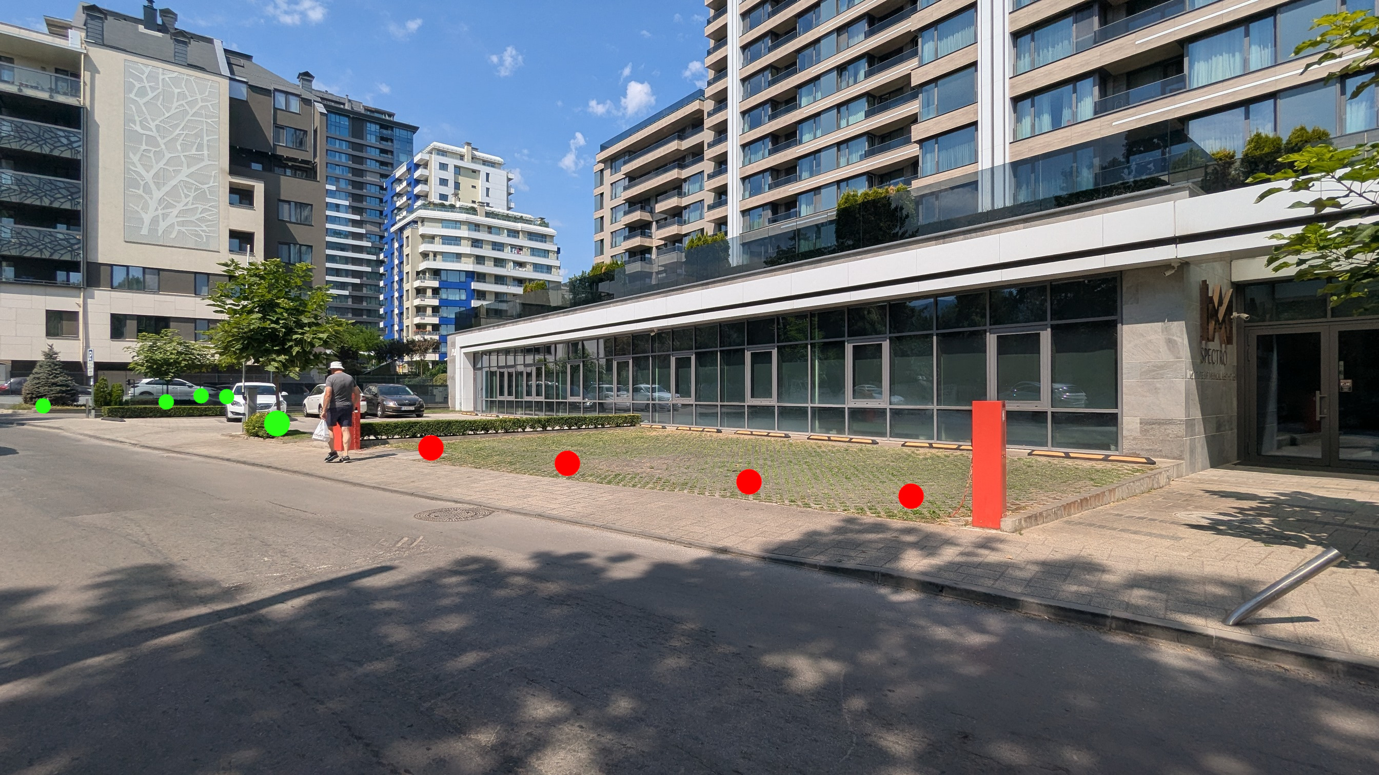
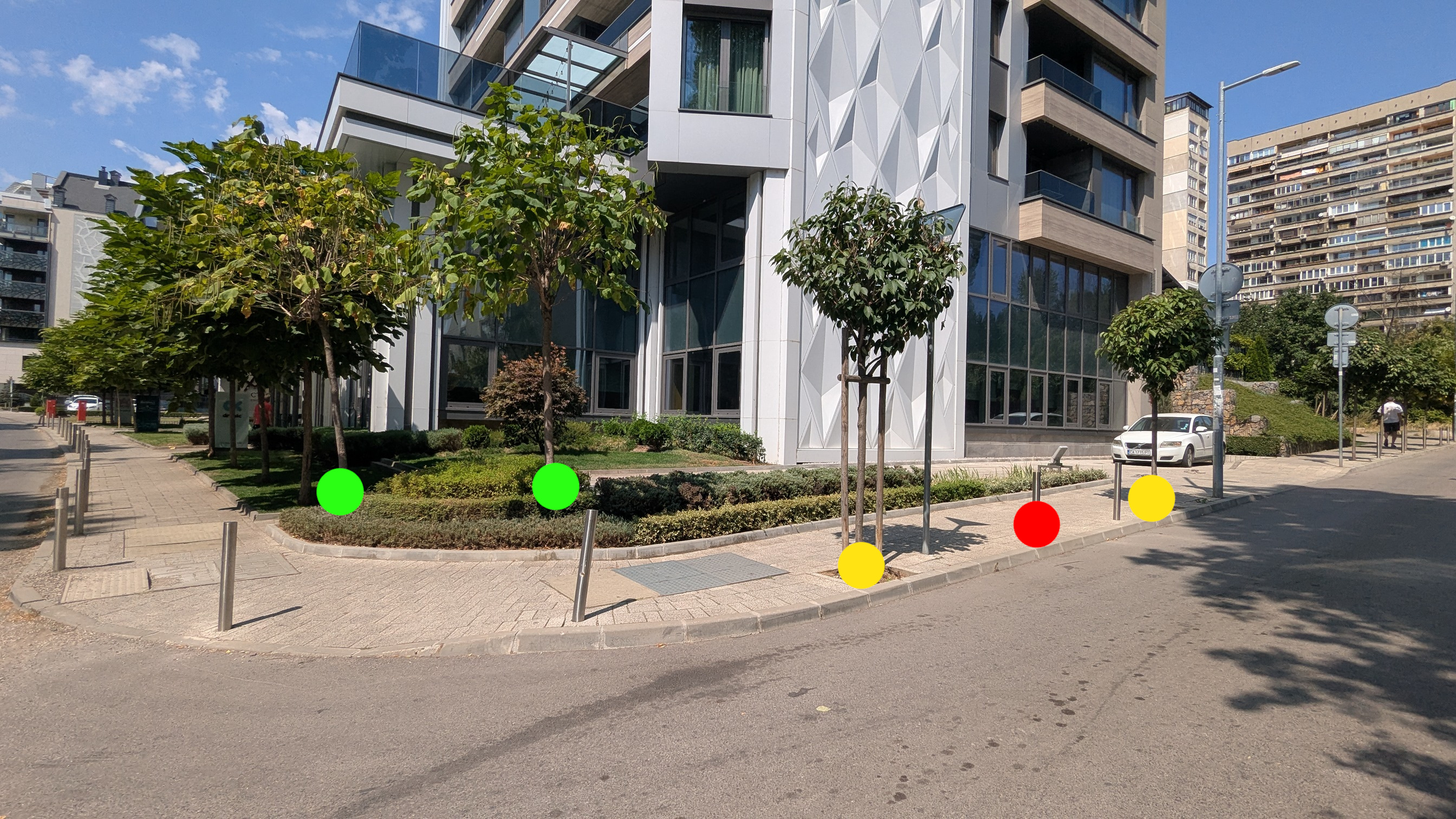
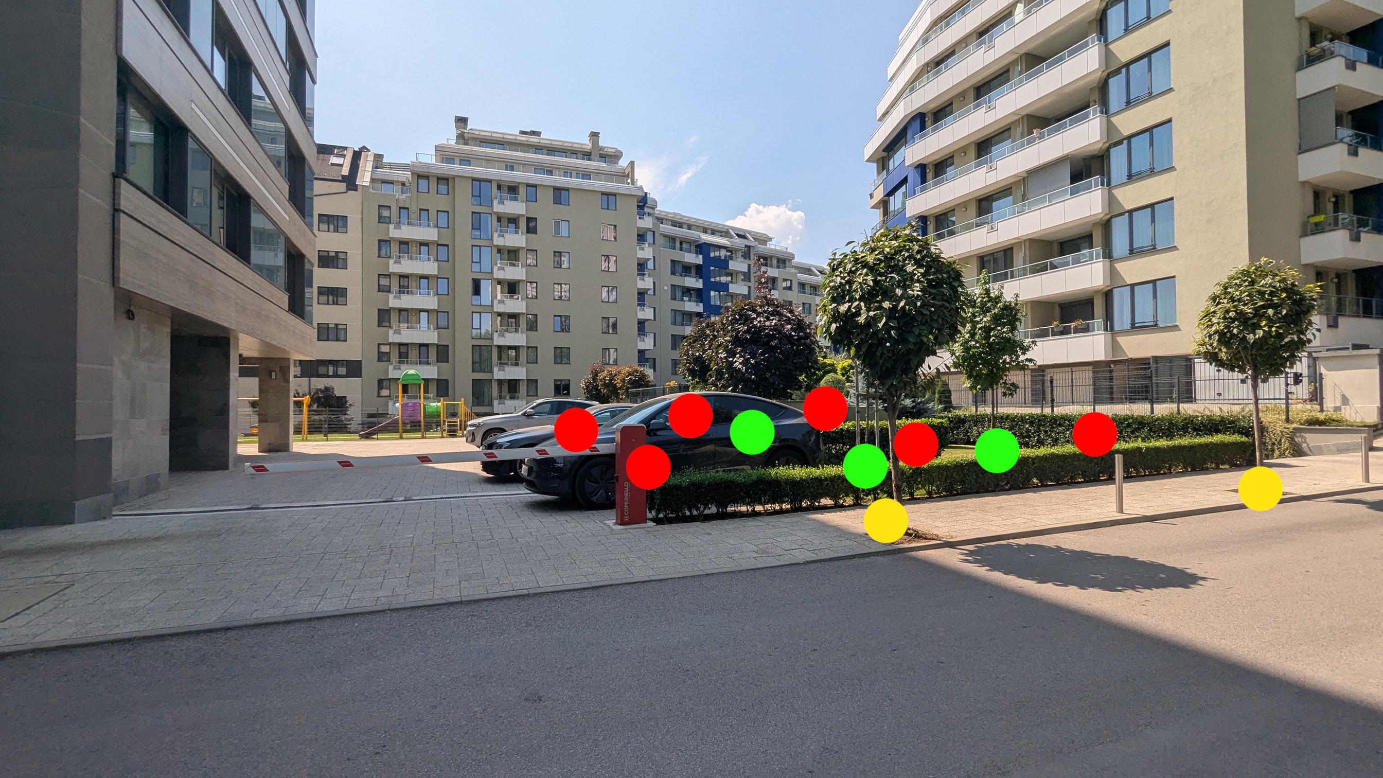
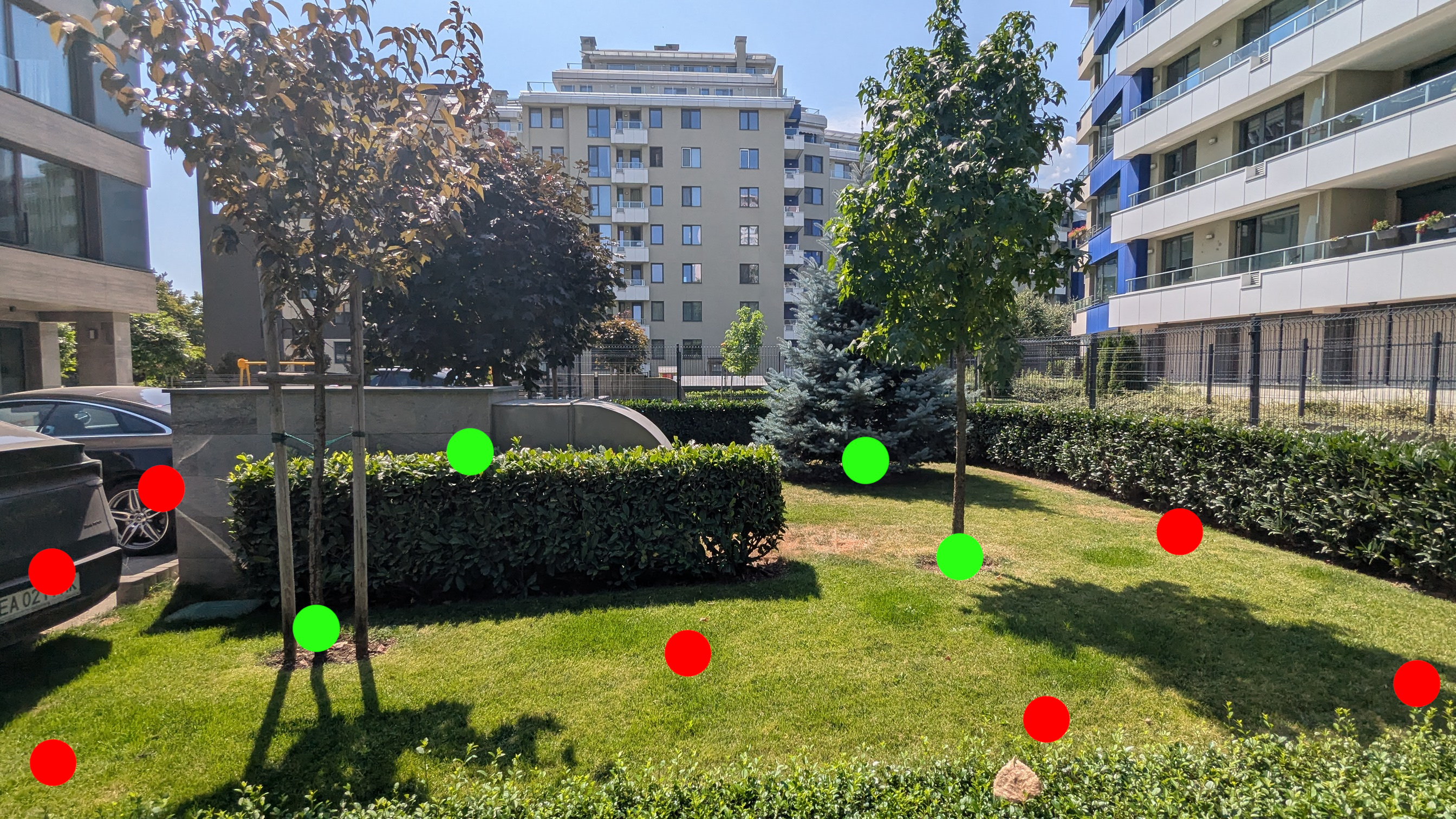
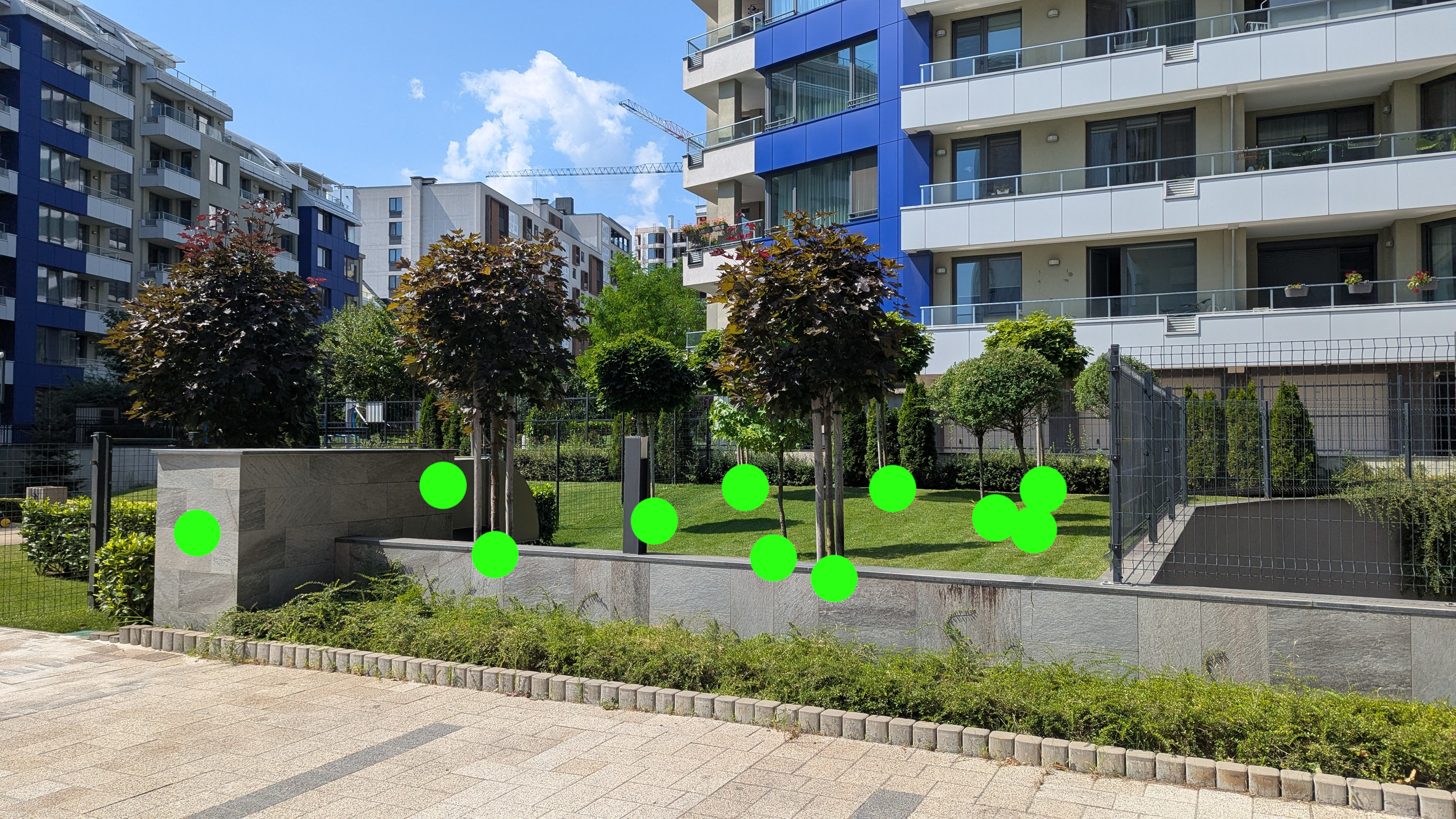
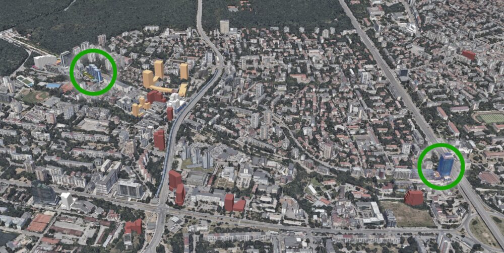
На снимката долу съм отбелязал първите два, на които се спрях – Диамант 2 и East Plasa Hotel. Тъй като предпочетох да съм изчерпателен, се налага да разделя примерите в два текста. Следващите два примера на сгради все още в строеж ще опиша утре. Снимките в галериите долу се сменят автоматично. Може да ги спрете с бутона за пауза горе вдясно.
Диамант 2

Сградата беше рекламирана като изключително зелена от инвеститора. Гледайки плановете за озеленяване, наистина изглежда така – 86 широколистни и 52 иглолистни дървета, 168 високи иглолистни храсти, над 6000 цветя и други храсти. Заявяват, че 41% от площта ще е в озеленяване, минимум 25% от която са високи дървета. Сградата се намира на поземлени имоти 68134.803.4008, 68134.803.4005 и 68134.803.4050 с обща площ малко над 7 декара. Те имат две отделни разрешителни за строеж с отделни изисквания за озеленяване. Това означава, че поне 2824 кв.м. от площта трябва да е в зеленина и трябва да има поне 59 високи дървета като минимум общо за двата строежа.

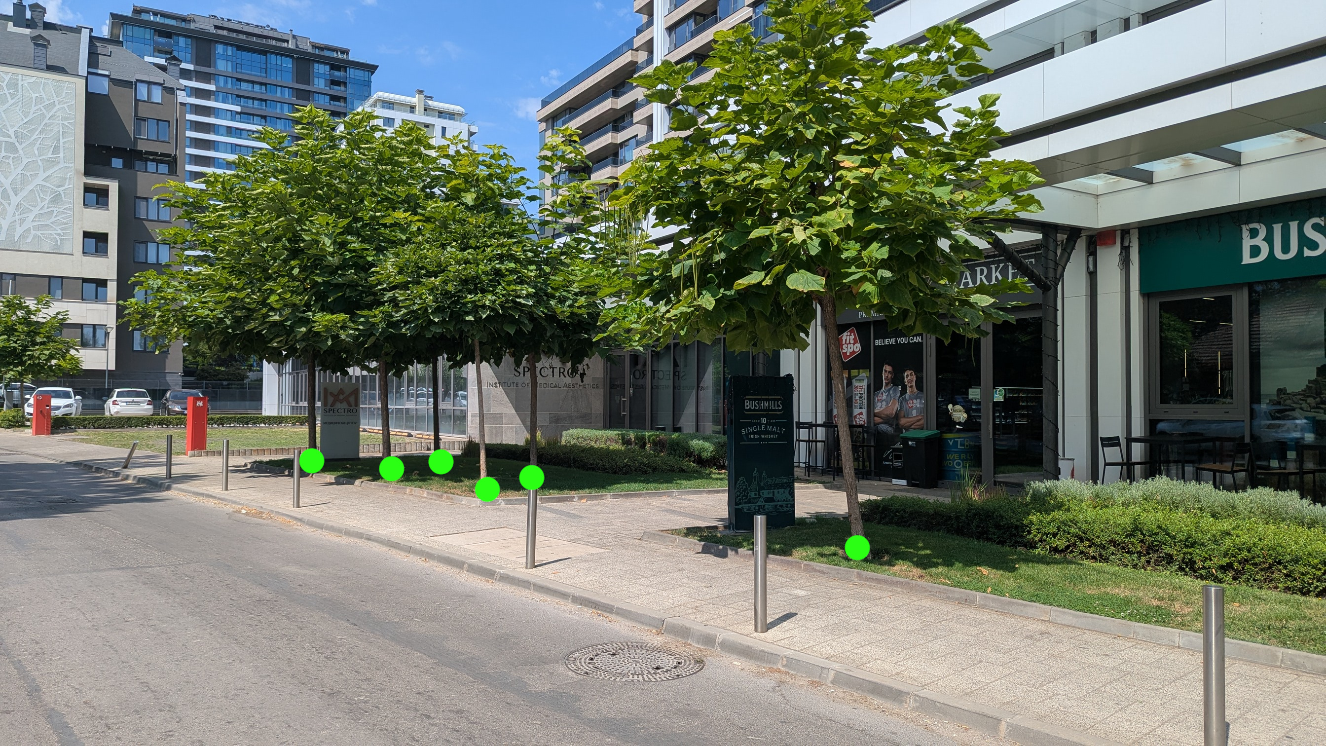
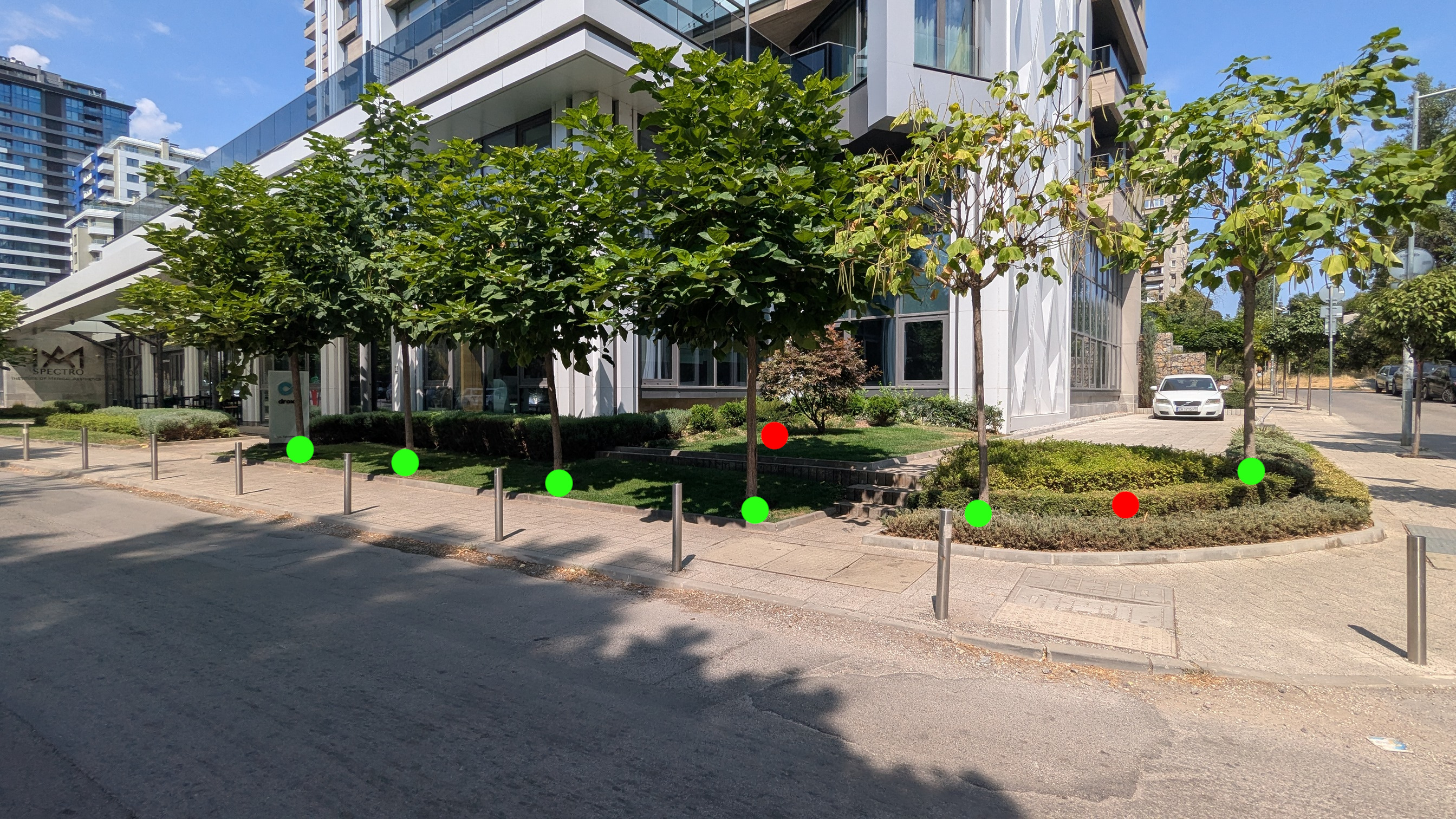
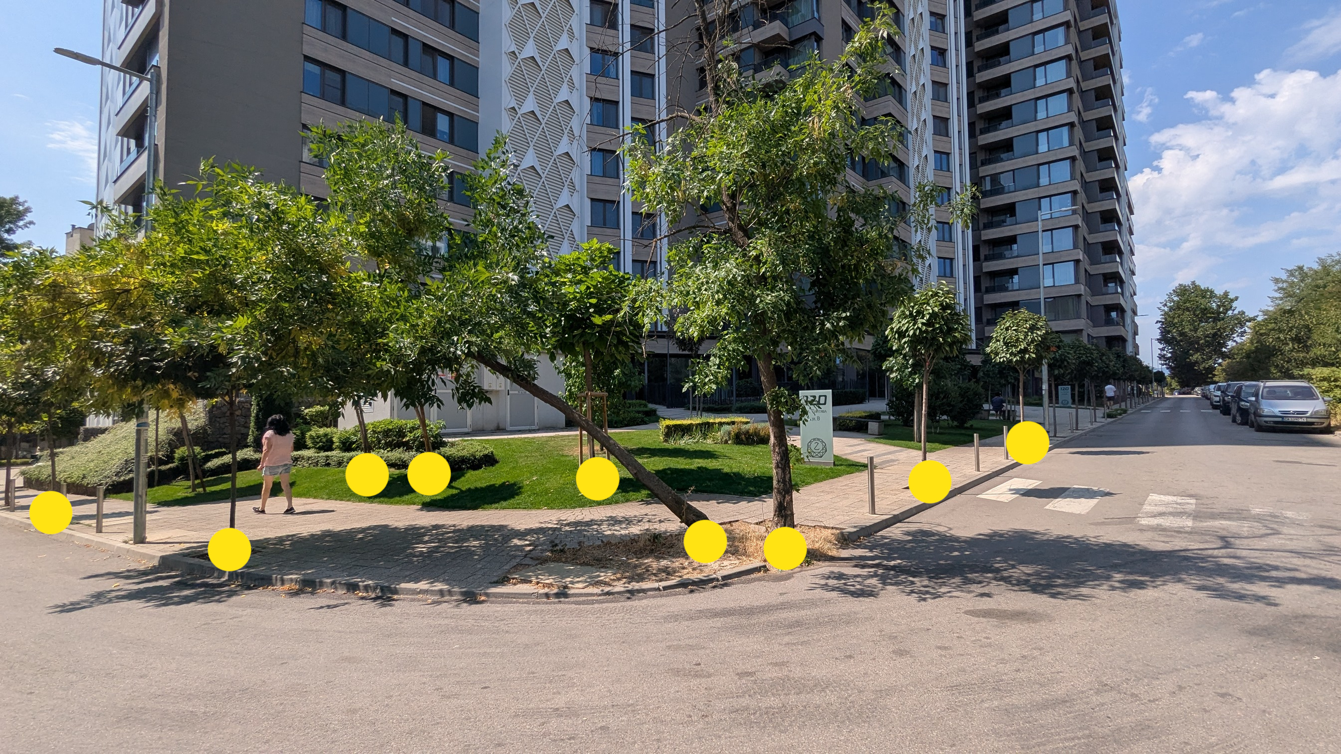
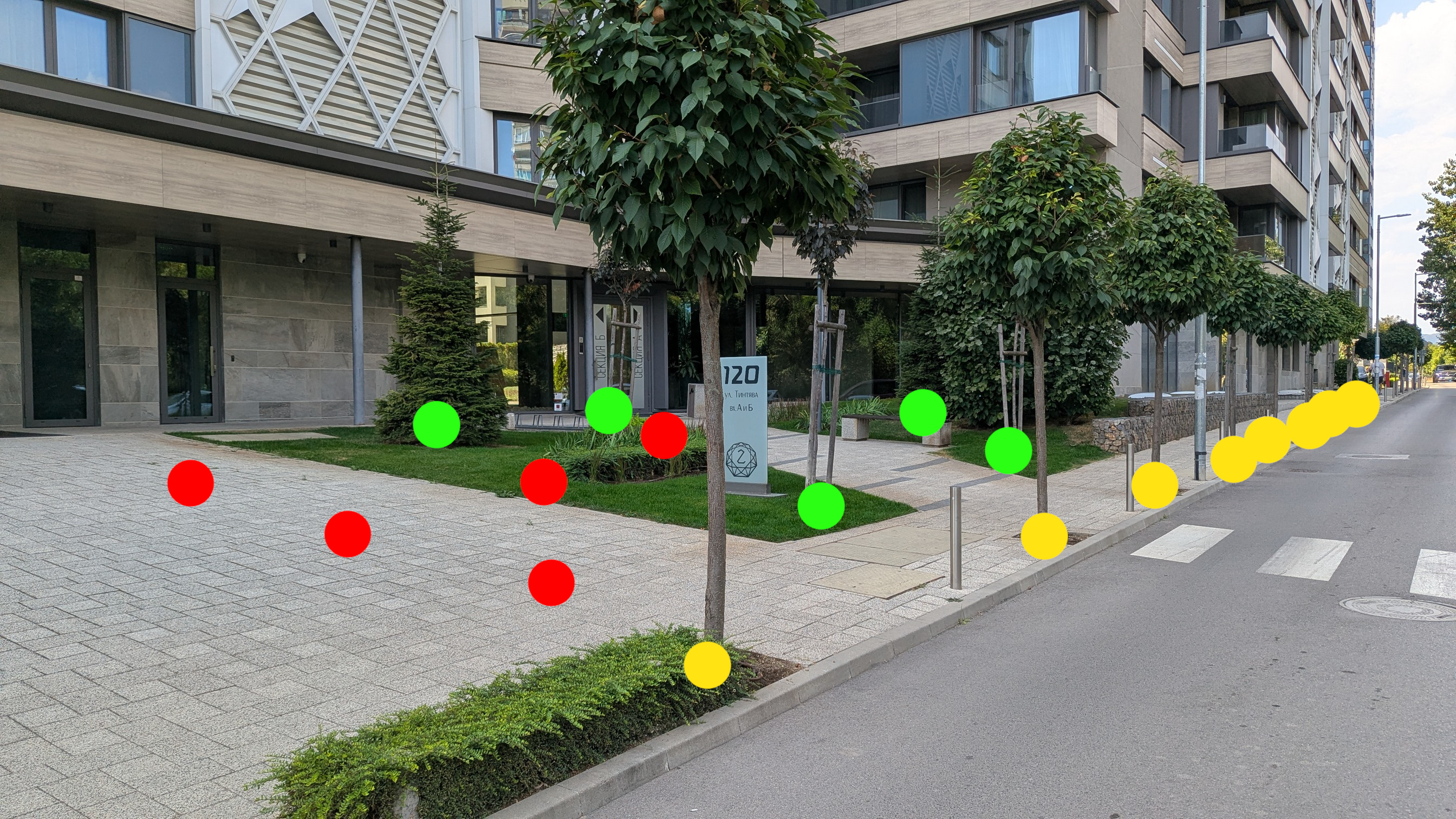
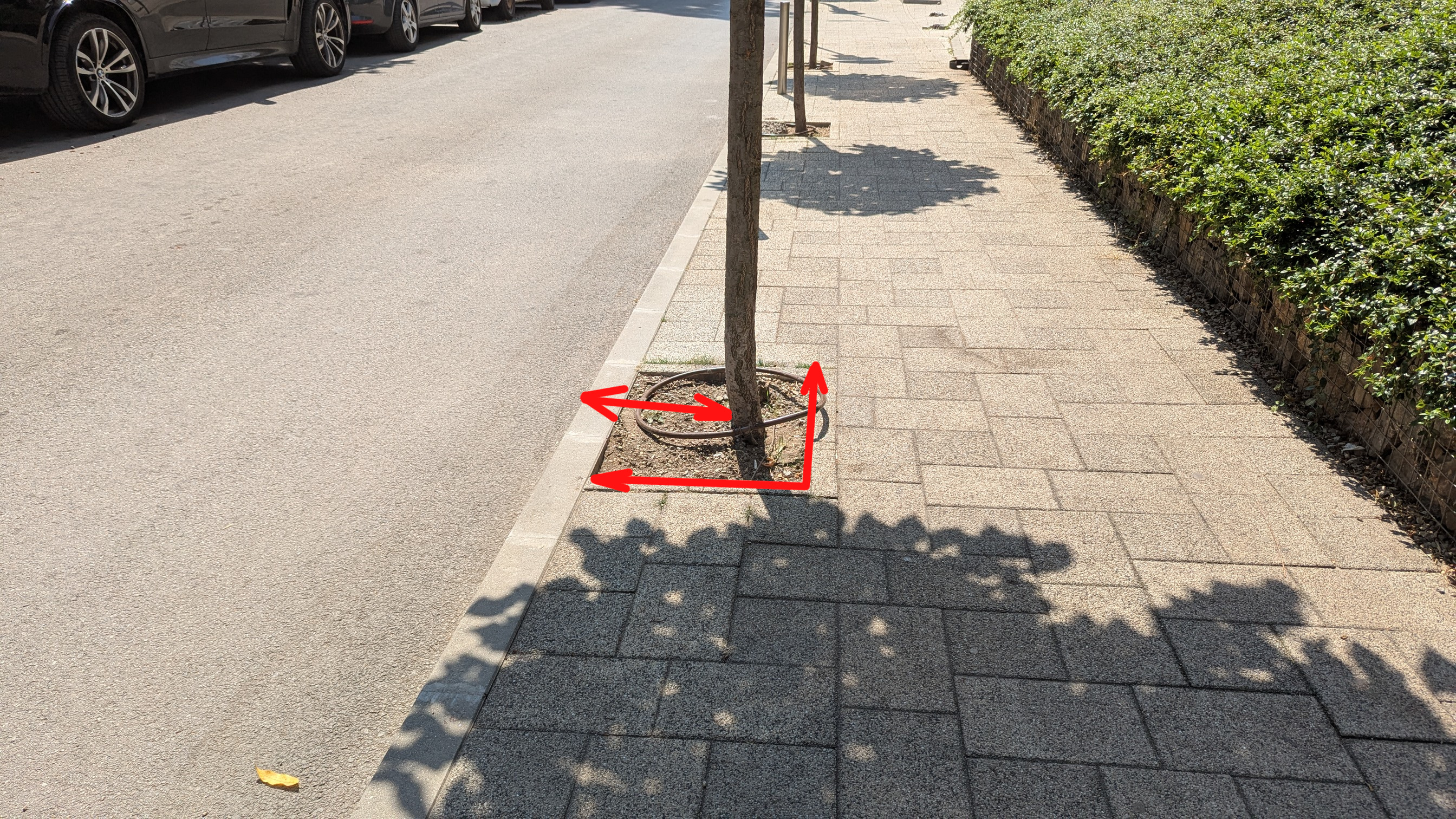
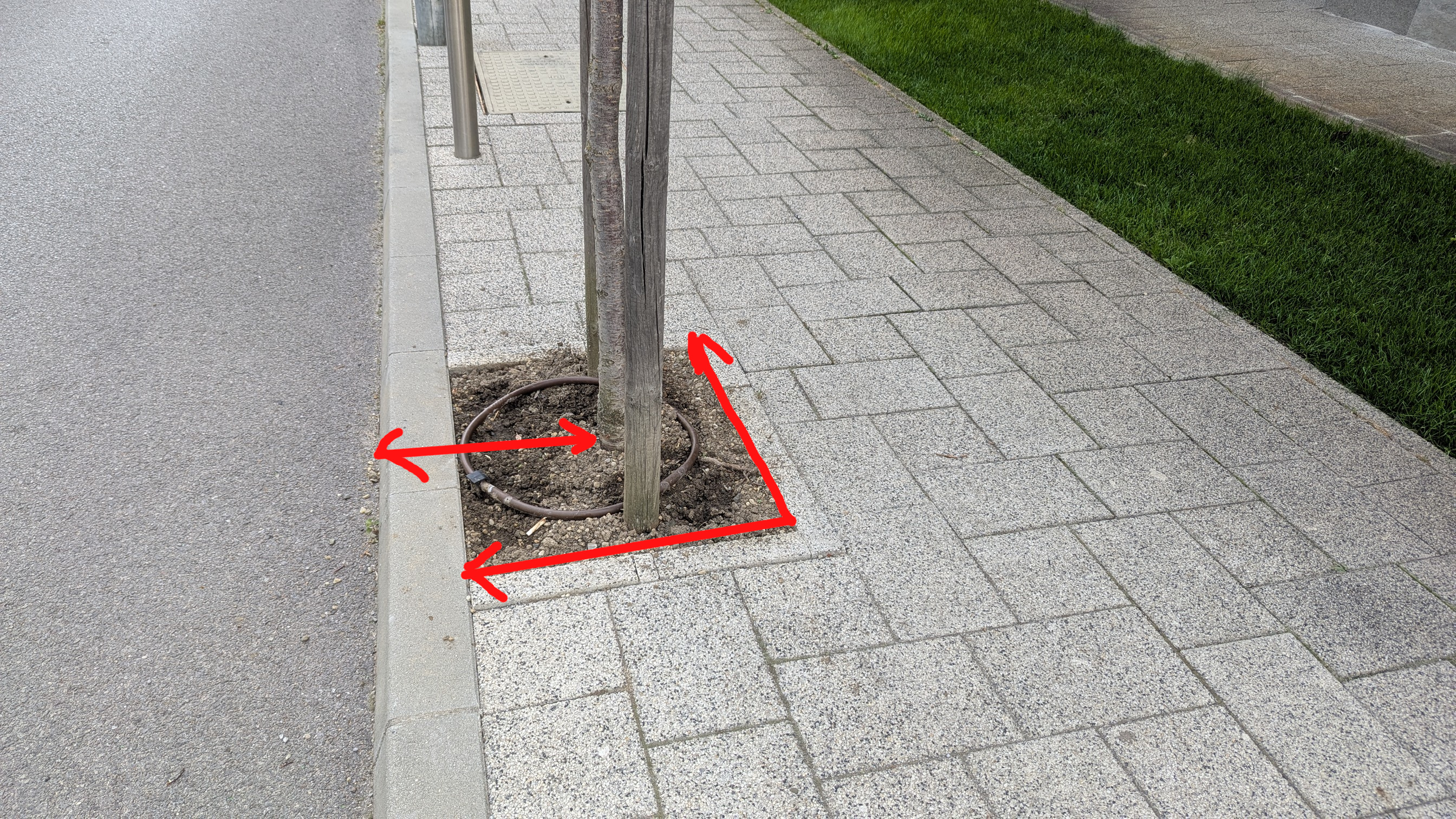
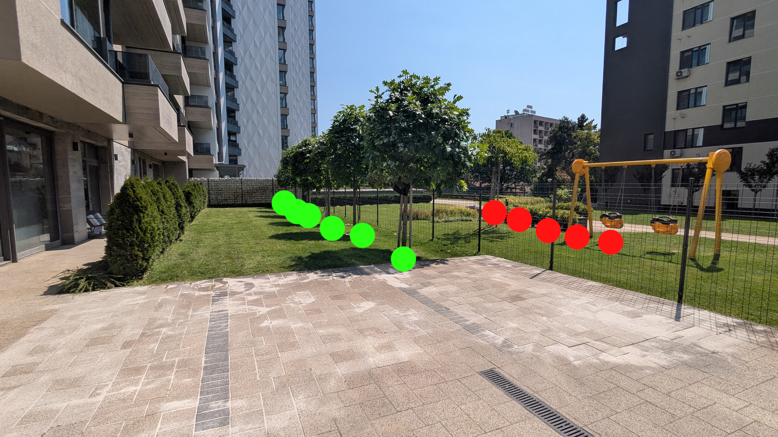
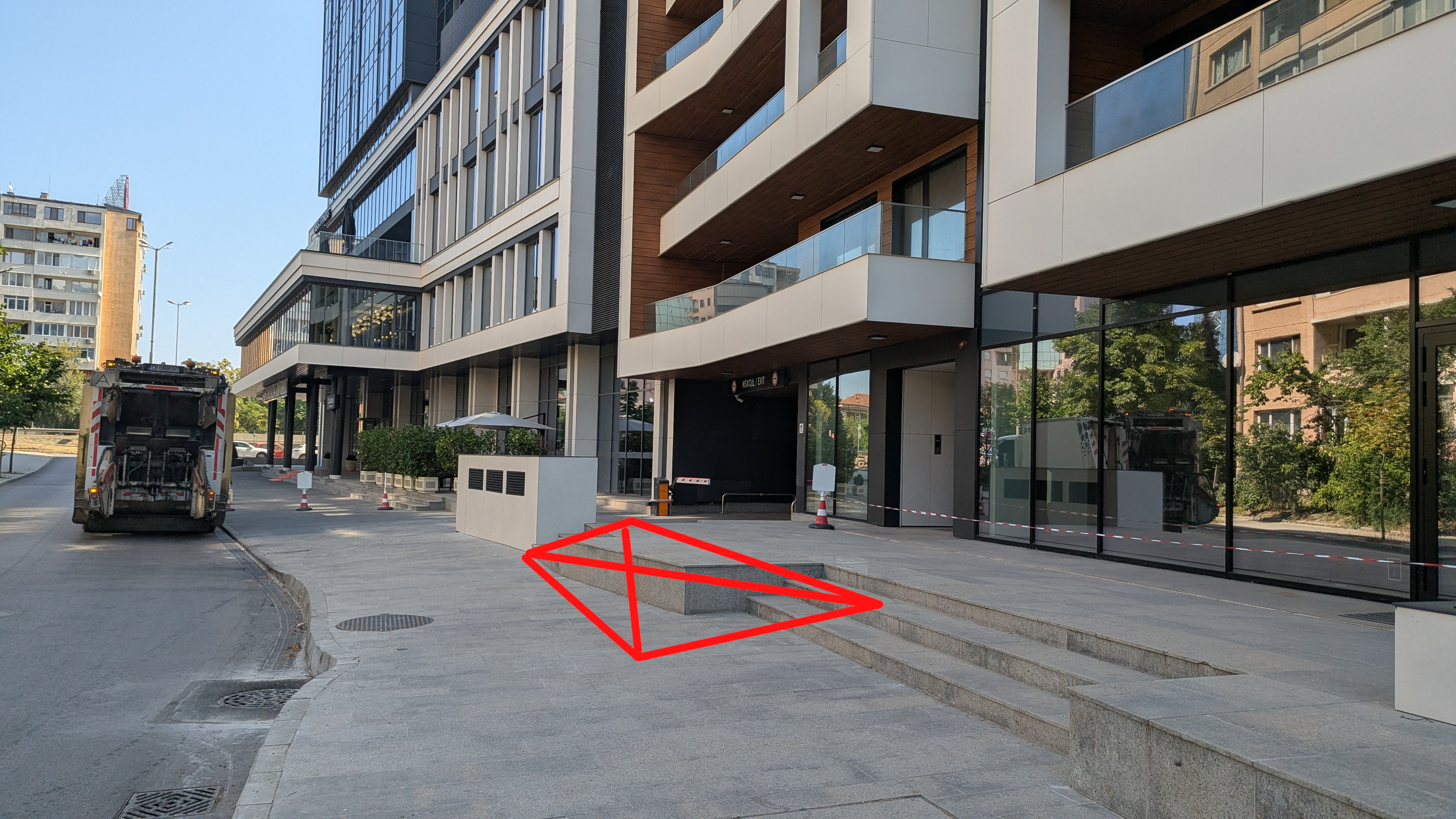
На място виждаме, че въпреки заявките на инвеститора, има 76 широколистни дървета, 7 иглолистни и не повече от 100 храсти от какъвто и да е вид. Отделно има 18 дървета, които не отговарят на изискванията, тъй като са долепени до бордюра с отстояние под два метра от улицата и под 70 см от тротоара (снимки 13 и 14 и всички отбелязани в жълто). Няколко други са твърде близо до фасадата или балкони, които отново ги дисквалифицира (снимка 16). Има още 23 дървета, които са всъщност в общински имот, който инвеститорът е на практика приобщил към комплекса (снимка 10). Там има и тяхна рекламна табела без разрешение за поставяне.

Споменатите над 40 дървета не може да се считат към озеленяването. От останалите обаче високите са не повече от 50, което е крайно недостатъчно, за да покрие изискванията. Друго любопитно нещо е, че половината са в първият етап на строежа, който е с отделно разрешение за строеж в парцел 4005. Там нещата изглеждат добре и отговарят на изискванията. Другият парцел 4008, който е значително по-голям и има отделно разрешение с отделно изчисление на озеленяването. Там липсват поне 55 дървета и коефициентът на високи дървета е значително под 25%.

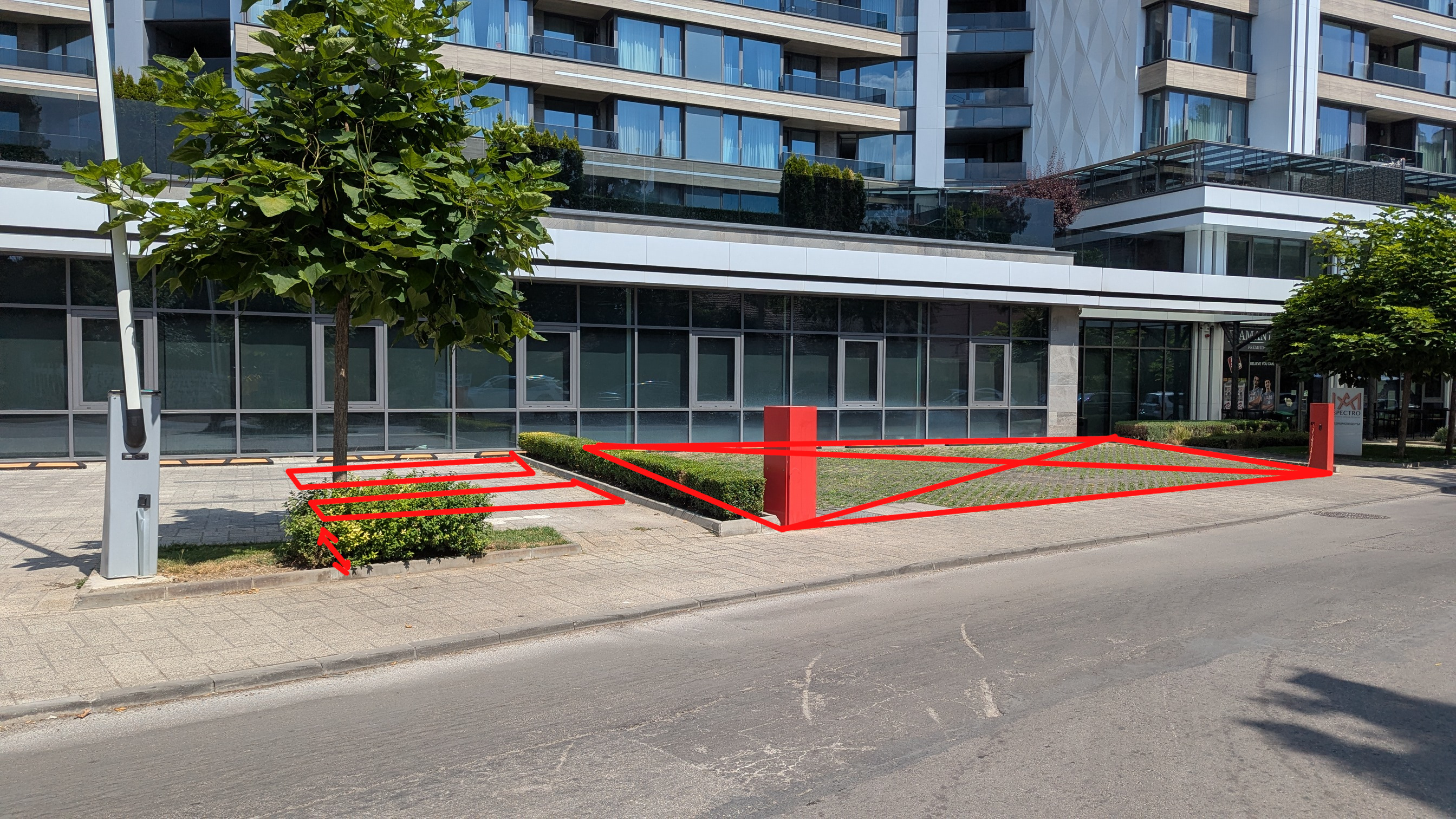
Отделен проблем е самата зелена площ. На много места се вижда, че почвата е не повече от 5 до 10 см. дълбочина. Изискването по старата наредба е поне 30 см. и 60 см. където има дървета и храсти. Пример за това е инцидент от 2024 г., когато едно от и без това малките дървета беше премахнато и част от градинката пред него беше превърната в паркомясто. Под него личеше, че е оставено малко малко дълбочина, но и това беше бетонирано и бяха сложени плочи направо на бетона симулираща, че има почва отдолу (снимка 4). В последствие след множество сигнали и месеци напомняне на районния кмет все пак върнаха дървото и сложиха трева. Дървото обаче сега е в малка вкопана кашпа, а тревата е с не повече от 5 см. почва под нея. Т.е. дефиницията на бутафорно озеленяване.

Аналогична е ситуацията вляво, където предвидена за зелена площ има отново бетонна плоча точно над паркингите и същите плочи за паркинг. Пред същото място по план трябва да има пет дървета, но има само едно, което също няма достатъчно отстояние или почва, за да оцелее. На това и на други места части от задължителното озеленяване е изчезнало спрямо когато са получили акт 16. В някои случаи това се е случило след година. В други – в рамките на последващи разрешения за строеж с цел промяна на предназначение, където е имало промени в озеленяването на имота. Последното е дори документирано от районната община като част от сигнали.

На няколко стари сигнала за описаните случаи районната община на Изгрев отговаряше, че всичко е наред и отговаря на проекта и изискванията. Отказваха на няколко пъти да предоставят плана за озеленяване като част от този проект. Сега разбираме защо – липсват десетки дървета и не са изпълнили дори базисните изисквания за отстояния, дълбочина на почвен слой и висока дървесна растителност. В крайна сметка пет годишният срок по ЗУТ от оригиналното разрешение за строеж, в който имат задължение да правят проверки изтече в началото на 2026 г.

За щастие, има две последващи разрешения за строеж на това място за преустройство на помещения с изходи към улицата – медицински център и магазин. Извинението на районната община този път е, че срокът от първото разрешение за строеж е изтекъл, а новите разрешения не предвиждали промени по озеленяването. Това не значи, че такива промени не е имало и отговори на стари сигнали го доказва. Изискване в последвалите разрешения за строеж е да не се променя нищо по имота, включително параметрите на озеленяването. Към него задължително се прилагат оригиналните планове.

Особеното тук е, че чл. 63, ал. 5 от ЗУТ не разграничава разрешенията за строеж и срокът от пет години започва да тече отново. Конкретно районната община следва да установи към днешна дата дали озеленяването отговаря като дълбочина на почвения слой във всички лехи, като брой дървета и отстояние на оригиналния план и изискванията. При липса на документация какво са установили при проверки между 2021 и 2024 г. единствената хипотеза е, че промените са се случили във връзка и след промените на предназначението на двата обекта. Това се подкрепя от случая в края на 2024-та, където именно това беше установено, но не и възстановено според изискванията. Тогава изрично районният кмет описа, че е ограничил проверката си до тези няколко квадрата и е установил проблем свързан с преустройството на магазина. Длъжен е да го направи за целия имот и има срок от още поне три години.

East Plasa Hotel

За разлика от предишната сграда, тази влиза в експлоатация през ноември 2024-та и районната администрация има задължение до края на 2029 г. да следи дали всичко отговаря на изискванията. Разрешението за строеж обаче е от 2019 г., т.е. важи старата наредба за озеленяването.

Тук първоначално е важало изискването за 40% озеленяване и това е отчетено в първите скици, които видях. Там предвиждаха значително по-малка интензивност на строежа, дървета и градинки по високите етажи и прочие. Заради един отчетливо лобисти текст в чл. 27 на ЗУТ това се променя. Имотът изкуствено се разделя на две през 2020 от Здравков. По-малката част е от страната на бъдещият зелен ринг и се застроява почти напълно (с изключение на 4 дървета от снимка 9). Така основната сграда се води ъглова, отпадат всички ограничения и успяват да постигнат тази височина и степен на застрояване. На практика сградата е една и без каквато и да е възможност за разграничение.

Все пак, в проекта, разрешението на строеж и при влизане в експлоатация твърдят, че имат 33.28% озеленяване, 34.75% от които са висока дървесна растителност. Това е важно, защото това би трябвало да видим на място и както сами се досещате не е съвсем така.

При дърветата има проблем, но не толкова голям, колкото при Диамант 2. По план трябва да имат 56 дървета. Десет от тях следва да по терасите на 6-тия етаж. Трудно се виждат, а височината и структурата на терасите не позволява да са спазени изискванията за кашпите. Трудно е, но нека предположим, че там всичко в наред.

С тях дърветата на място стават 50. Голяма част от тях не отговарят на изискванията за отстояние едно от друго или размер на кашпа или клоц (снимки 13, 14, 15 и 23). Същото важи впрочем и за храстите в снимки 16, 17 и 18. В края на 2024 г. имаше още едно място с озеленяване отбелязано на снимка 19, което обаче после беше бетонирано. Дори с тези липси обаче покриват сериозно намалените изисквания при условие, че дърветата на 6-тия етаж съществуват и си затворим очите за отстоянията и почвения слой.

Тук фрапантното нарушение е друго. За да постигнат дори малкия дял от 33.28%, тази сграда залага много на вертикално озеленяване. Това значи увивни и други растения, които покриват няколко пероги, вертикално по огради и стени на сградата. Общо в плана има 7 такива места, които да допринасят цели 48% от общия коефициент на озеленяване.

На място не виждаме нито едно от тези вертикални озеленявания. На снимка 3 виждате озеленяване, което трябва да е значително по-високо по оградата, но представлява ниски храсти с почвен слой от около 20 см. На снимки 4 и 11 виждате нещо, което е трябвало да бъде перога покрита изцяло в зеленина допринасяйки над 350 кв.м. към общото озеленяване. Това включва както по самата конструкция, така и вертикално на оградата пред нея и пълзяща още 160 кв.м. по стените наоколо. На снимка 12 виждате, че над дърветата по план е трябвало да има още озеленяване, вероятно на мястото на терасите, както и пълзящо по стените. На снимка 24 виждате място, където е трябвало да има над 120 кв.м. вертикално озеленяване по същия начин върху перога, което липсва.

Така изпълненото озеленяване не надвишава 20% дори с много уговорки за недостатъчния почвен слой. В края 2024, но преди пускането в експлоатация имаше сигнал, че почти готовата сграда видимо не може да отговаря на изискванията на озеленяване, че кашпите са твърде малки и плитки, а дърветата и храстите няма как да оцелеят и да се развият. Тогава отговорът от районната администрация беше, че щели да видят като е готово. Месец по-късно са подписали протокол като част от приемателна комисия, че всичко е наред. Поисках този протокол като административен акт на публична институция, но районната община ми отговори, че го нямали, което не би следвало да е вярно. Поисках го от ДНСК, които също отказаха, защото засягало интересите на инвеститора, а той изрично отказал да бъде публикуван. Обжалвах това решение в съда и предстои заседание.

Под тази сграда ще минава скоро новият Зелен ринг. Липсата на озеленяване и способност да се задържа дъждовна вода означава, че рингът ще се превръща в река. Това вече се случва постоянно на улицата пред въпросния хотел. При последните дъждове беше толкова зле положението, че зеленикавата вода влезе право във фоайето на хотела (снимки 29 и 30). Въпросната отсечка от улица Тинтява, но само до входа на гаражите на въпросния хотел, както и паркът срещу хотела (снимки 27 и 28) бяха ремонтирани приоритетно с публични средства от районната община. На въпроси от жителите на района беше настоявано, че няма връзка. Същият хотел има проблем и с огромният видео билборд, който е незаконен по три различни начина (снимка 26). Сигналите към районният кмет отново остават без отговор.

Какво от това?

Това са само два примера, но типични за новото строителство в София и в цялата страна. Често изниква въпросът има ли възможност да се засичат тези проблеми още докато се строи сградата. Отговорът често е да. Доколкото озеленяването се „забожда“ и „постила“ малко преди пускане в експлоатация, много преди това се разпознават плитките кашпи, бетонните плочи на нивото на бъдещата зелена площ, липсата на резервоари за дъждовна вода или въобще място за дървета. Затова в следващата част ще споделя два примера на строящи се сгради с подобен преглед и сравнение с плана им.

Несъмнено задължение е на приемателната комисия да разпознае тези проблеми предвид, че има експерти в нея. От примерите виждаме, че това не се случва. Натрупването на такива случаи води пряко и непряко до доста от проблемите в градска среда, включително риск за безопасността и здравето на хората. Никой строеж сам по себе си не е виновен за това, но в съвкупност общото нехайство, неспазване на изискванията и дори грубо нарушаване на закона прикривани със съмнения за корупция допринасят до това, което наричаме презастрояване.

Разбира се, единствено циничността като типично българско качество ни води към предположението, че е намесена корупция. Не може да твърдим, че подобни практики е имало при който и да е от описаните тук примери. Ако прочитът ми на документите е неправилен, което би било също разумно предположение, то не може да говорим дори за административно нарушение, с което се изчерпва личното ми мнение относно разминаването между видяното на място и плановете, до които ми беше даден достъп.

Очаквайте утре следващата част от темата с още такива примери. В първата част от серията бях описал трудностите да стигна до тези документи.

Data Mesh at Grab (Part III): Operationalizing data reliability with automated DPIs

Post Syndicated from Grab Tech original https://engineering.grab.com/data-mesh-at-grab-part-three

Introduction

In the first two parts of this series, we described how Grab approaches data mesh through the Signals Marketplace: a way for teams to publish, discover, and reuse trusted data products across domains. Part II introduced the foundational tools behind certification: Hubble for metadata and ownership, Genchi for data quality observability, and the Data Contract Registry for explicit producer-consumer guarantees.

Certification is the starting point for a trusted data marketplace. It gives downstream consumers confidence in an asset’s ownership, documentation, lineage, and quality controls. Certification does not eliminate runtime failure. A certified table can still arrive late. A certified metric can still be affected by a broken dependency. A certified Kafka stream can still violate a freshness expectation.

Keeping certified data products reliable in production requires more than defining standards upfront. Teams need a consistent way to detect failures, diagnose the root cause, fix the issue, and verify recovery. That is where Data Production Issues (DPIs) come in. At Grab, DPIs turn data quality signals into an operational workflow.

The DPI lifecycle

A good DPI should be clear enough to act on, and it should close automatically when the underlying condition recovers. From the beginning, we designed the DPI lifecycle to be automated, with minimal human-in-the-loop.

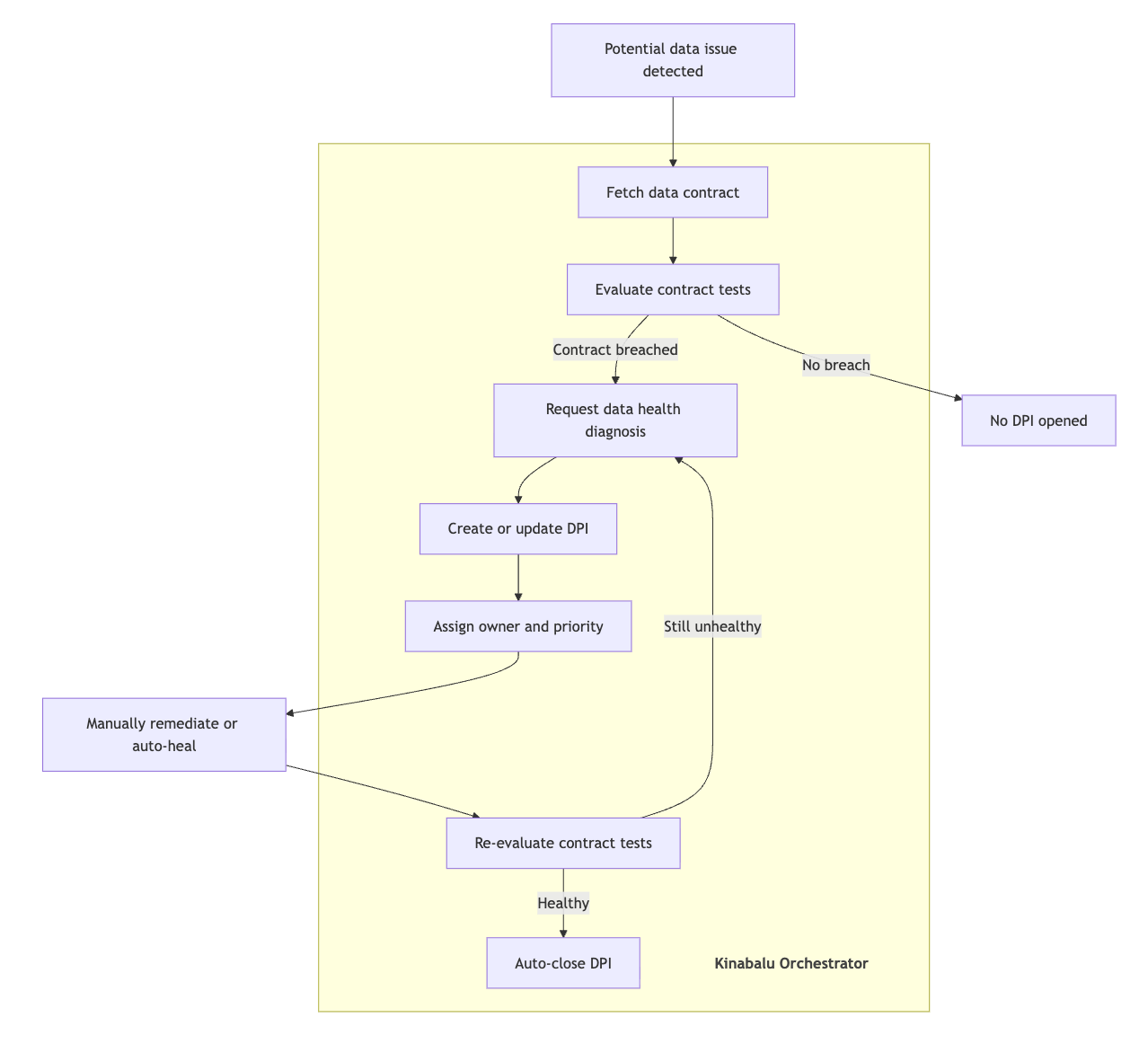
The lifecycle starts when Kinabalu, Grab’s incident orchestrator, observes that a data asset may no longer satisfy its contract. The contract captures the reliability expectations that matter for the asset, along with the health checks, exposed through Test Health application programming interfaces (APIs), that evaluate those expectations.

The orchestrator stays decoupled from platform internals. It does not need to know how each platform computes freshness, completeness, or other quality dimensions. It only needs to ask whether the relevant contract tests are healthy. If one or more contract tests are unhealthy, the contract is considered breached, and the DPI lifecycle begins.

Diagram of the automated Data Production Issue workflow from contract-test evaluation through triage, diagnosis, resolution, and close.
Figure 1. Automated DPI workflow.

Triaging DPIs: From alerts to confirmed contract breaches

Data platforms emit many alerts. An Airflow schedule may be delayed, a data quality test may fail, or a pipeline job may exit unexpectedly. These alerts are useful, but they are not automatically DPIs. Triage decides whether an alert represents a real contract breach for a data asset.

As introduced in Part II, a data contract is an explicit, versioned agreement between a data producer and its consumers. It outlines the data’s schema, freshness, completeness, and other semantic guarantees. These guarantees are codified and enforced through data quality tests in Genchi.

When the incident orchestrator evaluates contract tests, it distinguishes an individual test run result from the overall health of a test. A test run can pass or fail at a point in time, but the test itself may only be considered healthy after the underlying issue has been fully resolved. For example, consider a completeness test that checks whether the T-1 daily partition is complete. If the test failed two days ago but passed yesterday and today, the test may still be considered unhealthy until the partition from two days ago has been backfilled and verified as complete.

The orchestrator also deduplicates around the active unhealthy condition. If an asset already has an open DPI for the same breach, new signals update the existing DPI with additional context rather than creating parallel issues. DPIs that share the same underlying root cause can also be grouped. This keeps responders focused on solving the underlying issue rather than chasing a stream of repetitive alerts.

During triage, the workflow also gathers context for the DPI: affected asset, breached contract, unhealthy tests, data interval, and upstream and downstream dependencies. Not every alert becomes a DPI. Triage protects the operational workflow from noise by promoting only meaningful contract breaches into production issues.

Diagnosing DPIs: Assigning owners with root cause analysis (RCA)

Once a DPI is created, the system must answer why the data is unhealthy, who should fix it, and how.

Not every data issue should be assigned to the data asset owner. A data product may be unhealthy because of a platform incident, a failed producing job, or a delayed upstream dependency. Assigning every issue to the asset owner creates unnecessary handoffs and slows down resolution.

This is where the Data Health API matters. It answers the question: “What kind of failure made this asset unhealthy?” The Data Health API keeps the error taxonomy small:

  • UPSTREAM_ERROR: the asset is unhealthy because an upstream dependency is late, failed, or unavailable.
  • PLATFORM_ERROR: the asset is unhealthy because the underlying platform or infrastructure is impaired.
  • JOB_ERROR: the asset is unhealthy because the producing job or pipeline failed.
  • DATA_ERROR: the asset is unhealthy because the produced data violates quality expectations.

The taxonomy is not meant to replace platform-specific diagnostics. The high-level Data Health API gives the orchestrator just enough structure to assign DPIs and manage their lifecycle consistently. An ingestion platform, streaming platform, metrics platform, or machine learning (ML) platform can still maintain detailed internal error catalogs, logs, retry states, and debugging tools. Platforms remain free to evolve their internals, while the incident orchestrator consumes a stable API contract, so the DPI workflow can interoperate across heterogeneous systems.

A simplified Data Health API response might look like this:

Disclaimer: The fields in this API response are mock data generated for demonstration purposes and do not represent real operational metrics.

{
  "assetId": "urn:li:dataset:(urn:li:dataPlatform:hive,schema.table_A,PROD)",
  "healthStatus": "UNHEALTHY",
  "errorCategory": "UPSTREAM_ERROR",
  "context": {
    "upstreamAsset": "urn:li:dataset:(urn:li:dataPlatform:hive,schema.table_B,PROD)",
    "reason": "upstream data has not arrived for the expected data interval."
  },
  "lastCheckedAt": "2026-06-15T08:30:00Z"
}

From this response, the orchestrator can see that table_A is unhealthy because of an upstream dependency rather than a problem in the asset itself. It then traces the active DPI for the upstream asset and links the table_A DPI to that upstream issue. The downstream DPI can inherit the same owner as the upstream DPI, keeping related failures grouped under the team best positioned to resolve the root cause.

The DPI process works only when the issues it raises can be assigned and fixed. If DPIs are frequently noisy, duplicated, or difficult to act on, users will eventually learn to ignore them. Diagnostic accuracy matters because it keeps DPIs useful for the people who receive them. It also creates a forcing function for each data-producing platform to improve its diagnostics. To produce accurate RCA, platforms need to incorporate signals from their dependencies and surrounding systems, not just their own local failure state.

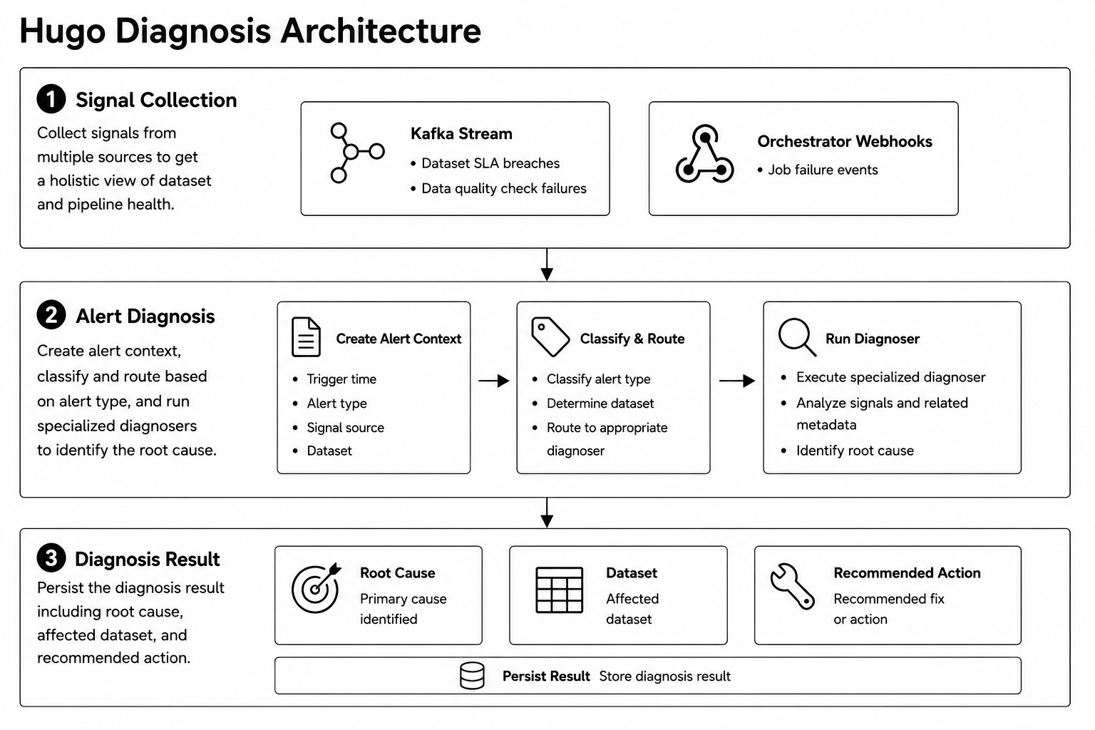
Grab operationalizes DPI diagnosis across its internal data platforms. Our ingestion platform, Hugo, is a primary example of this approach, as outlined in a previous tech blog. Hugo’s intelligent diagnosis architecture uses a three-layered system to automatically detect, analyze, and troubleshoot data pipeline failures within its domain, as shown in Figure 2.

Diagram of Hugo's three-stage diagnosis architecture: signal collection, alert diagnosis, and diagnosis result.
Figure 2. Hugo diagnosis architecture.

Modern data platforms generate alerts from many independent systems. Individually, these signals show only a partial view of a dataset. Hugo consolidates platform-specific signals into a unified diagnostic workflow to pinpoint root causes and recommend pipeline remediations. The diagnosis architecture consists of three stages:

  1. Signal collection collects events from multiple signal sources to build a full view of the dataset and pipeline health.
  2. Alert diagnosis creates a structured alert context, classifies the alert, routes it to the appropriate diagnoser, and identifies the root cause using specialized diagnosis logic.
  3. Diagnosis result persists the structured diagnosis output, including the identified root cause, affected dataset, and recommended fix or action.

For example, when a dataset fails, the workflow orchestrator notifies Hugo with a job failure event. Hugo then routes the alert to its internal diagnostic layer to check for conditions such as upstream database replica lag, storing both the diagnosis and recommended fix alongside the affected dataset.

Decoupling signal ingestion, diagnosis, and result management makes it straightforward to add new signal sources and specialized diagnosers. Immediate RCA removes the need for manual log inspection, which shortens remediation and feeds directly into automated resolution workflows.

Resolving DPIs: Auto-healing first, human judgment when needed

After triage and RCA, the final stage of the DPI lifecycle is resolution. The lifetime of a DPI is a proxy for data downtime: it begins when a contract breach is detected and ends when the affected dataset becomes healthy again. Reducing that window requires more than identifying the correct issue. It also depends on recovering safely and consistently from recurring failure modes.

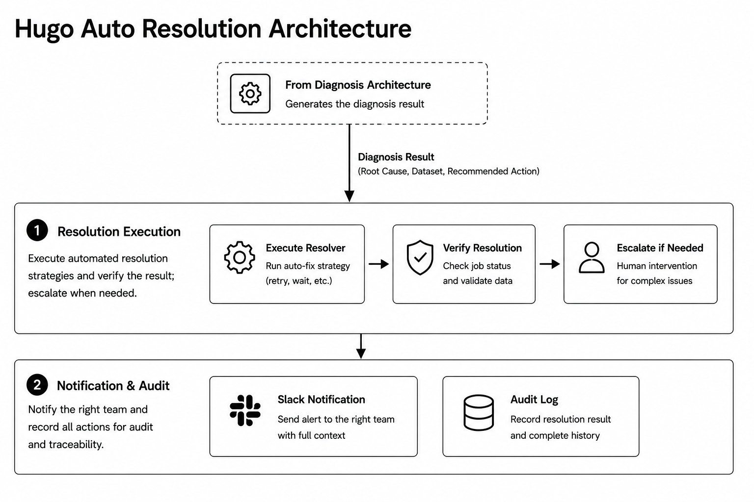
Many incidents are routine and recoverable, such as transient compute interruptions, database connection timeouts, S3 throttling, or upstream pipelines that are delayed rather than permanently broken. Instead of relying on manual intervention for every incident, Hugo automates recovery for these well-understood failure patterns. Once the diagnosis workflow identifies the root cause, it produces a structured diagnosis result containing the affected dataset, the root cause, and the recommended resolution strategy. The auto-resolution workflow then consumes this result to execute the appropriate remediation automatically. Figure 3 shows Hugo’s auto-resolution architecture in two stages.

Diagram of Hugo's auto-resolution architecture, covering resolution execution plus notification and audit.
Figure 3. Hugo auto-resolution architecture.
  1. Resolution execution applies the recommended resolution strategy, such as retrying a failed job, waiting for an upstream dependency, or executing a custom resolver. After the action completes, the system verifies both pipeline health and data correctness to confirm the issue has been fully resolved. If a failure cannot be resolved safely through automation, such as in cases of data corruption, invalid records, or application code defects, the workflow escalates the incident for human intervention.

  2. Notification and audit records every resolution attempt and its outcome, while notifying the appropriate engineering teams. That record supports operational analysis, auditing, and later improvements to resolution policies.

For example, a dataset may miss its freshness Service Level Agreement (SLA) because the workflow orchestrator becomes temporarily unresponsive and fails to submit the scheduled ingestion job. The diagnosis workflow identifies the incident as a pipeline execution failure and recommends a retry strategy. Hugo automatically retries the job, verifies that the pipeline completes and data health is restored, then logs the recovery and notifies the responsible team. This end-to-end process, from incident detection to resolution, runs automatically without manual intervention.

Hugo closes the loop between detection, diagnosis, and recovery. Rather than stopping at identification, the platform turns diagnosis results into targeted remediation, so routine operational issues can be resolved automatically while preserving human oversight for complex or high-risk incidents. Separating diagnosis from execution also lets new diagnosis capabilities and resolution strategies evolve independently without changing the overall architecture.

The impact is already evident in production. 86.9% of DPI incidents were automatically resolved, significantly reducing manual operational effort. By automating routine recoveries, engineers spend less time performing repetitive operational tasks and more time building new platform capabilities, while overall data downtime is significantly reduced.

Conclusion

Certified data products still need to prove their reliability in production. Freshness delays, upstream failures, platform incidents, and data quality violations can all break consumer trust, even when an asset has already met certification standards.

Automated DPIs are the operating model for managing these failures. By turning contract breaches into structured production issues, the DPI lifecycle makes data reliability operational: triage separates real breaches from alert noise, diagnosis identifies the likely failure domain, ownership routing reduces handoffs, and resolution closes the loop through auto-healing or human intervention when needed.

The most important outcome is not simply that issues are detected faster. It is that data downtime becomes visible, measurable, and reducible. With every DPI tracked from detection to recovery, teams can understand where time is spent, which failure modes repeat, and where automation can safely reduce operational toil. To date, more than 95% of DPIs are raised automatically rather than by humans, with a mean time to resolve (MTTR) that is 6 times faster for automated DPIs than for manually raised ones.

For Grab, this shifts data reliability from reactive firefighting to a managed production workflow. Automated DPIs help keep trusted data products trustworthy after certification, so downstream teams can depend on them with greater confidence.

What’s next

Across the three-blog series, the story is how Grab turns data mesh from an operating principle into an artificial intelligence (AI)-ready foundation for the company.

  • Part I: Building trust through certification. Grab needed the Signals Marketplace because the business had scaled across mobility, deliveries, financial services, and many data-producing domains. The old model of relying on a central Data Engineering team could no longer keep up. Certification became the mechanism for making high-quality data products visible, reusable, and accountable. With clear ownership, data contracts, and measurable adoption, Grab moved more consumption toward trusted assets, reduced duplication, and created stronger incentives for teams to curate the data they publish.

  • Part II: The foundational tools behind certification. Trust becomes operational through platforms. Hubble covers discovery, lineage, ownership, and the certification engine. Genchi runs continuous data quality observability across freshness, completeness, schema, and business-rule checks. The Data Contract Registry formalizes producer-consumer expectations as versioned, enforceable contracts. Combined, these systems keep data certification an actively maintained standard rather than a static label.

  • Part III: Operationalizing data reliability with automated DPIs. Certification tells consumers which data products should be trusted; DPIs keep that trust true in production. Kinabalu evaluates contract breaches, deduplicates noisy alerts, assigns ownership, and tracks recovery. Data Health APIs make RCA portable across platforms, while Hugo’s diagnosis and auto-resolution patterns show how common failures can be remediated faster and with less operational toil. The result is a measurable reduction in time to resolve and a stronger feedback loop back into certification.

The bigger takeaway is that Grab’s data moat is not just the volume of data we have. It is the system that makes our data trustworthy, discoverable, reusable, and continuously reliable. This foundation is what lets us embrace the agentic world: AI agents can search certified assets, reason over contracts and lineage, trust quality signals, detect production issues, draft RCA, and eventually suggest or execute safe remediation. In that world, data reliability becomes a compounding advantage. The better our foundations are, the more confidently Grab can build agentic experiences on top of them.

We would like to thank all the data practitioners across Grab, including engineers and analysts to data scientists and product teams, who have invested in certification, contracts, and data quality to build a solid foundation for AI agents and AI-powered experiences. We are equally grateful for the unwavering sponsorship, strategic guidance, and hands-on support from our leadership (Mohan Krishnan and Nikhil Dwarakanath), without which this long-term data foundation initiative would not have been possible.

Join us

Grab is Southeast Asia’s leading superapp, serving over 900 cities across eight countries (Cambodia, Indonesia, Malaysia, Myanmar, the Philippines, Singapore, Thailand, and Vietnam). Through a single platform, millions of users access mobility, delivery, and digital financial services, including ride-hailing, food delivery, payments, lending, and digital banking via GXS Bank and GXBank. Founded in 2012, Grab’s mission is to drive Southeast Asia forward by creating economic empowerment for everyone while delivering sustainable financial performance and positive social impact.

Powered by technology and driven by heart, our mission is to drive Southeast Asia forward by creating economic empowerment for everyone. If this mission speaks to you, join our team today!

How we saved 100 terabytes of memory by optimizing 1.1.1.1’s DNS cache

Post Syndicated from Sebastiaan Neuteboom original https://blog.cloudflare.com/dns-cache-memory-optimization-1111/

Big Pineapple, the platform behind 1.1.1.1, Gateway DNS, DNS Firewall, AS112, and several other Cloudflare DNS services, stores over 250 billion DNS cache entries at any given time. At that scale, wasting a single byte per entry costs more than 250 gigabytes of memory across our fleet.

Five successive changes to how cache entries are stored in memory cut the per-entry footprint by over 50%. Across our fleet, these changes freed up roughly 100 terabytes of memory, equivalent to the amount of RAM in 130 of our Gen 13 servers. The cache also got faster. Insert throughput rose 43% and lookup latency dropped 19%, as fewer allocations and better memory locality meant we did not trade speed for space.

What we cache

On cold start, Big Pineapple starts out with an empty cache. As DNS queries arrive, the cache fills until it hits its maximum entry count, at which point we evict older or less popular items to make room.

The exact cache size varies by data center. When EDNS Client Subnet (ECS) is in use, authoritative servers return different answers depending on the client's network, so we cache multiple versions of the same query. This increases both the number of entries and the memory each one consumes, making the optimizations in this post especially impactful for ECS-heavy locations.

Each item in the cache is a key-value pair. The key identifies what was queried:

The value stores the DNS response itself: the answer, authority, and additional record sections, along with metadata like the creation time, a hit counter, and the Time-to-Live (TTL).

Both structs have room for improvement. Several fields use types that carry overhead we don't need once the entry is stored.

Benchmarking memory usage

To measure the impact of each change, we benchmark by filling the cache with randomly generated entries that roughly match the traffic distribution we see in production: 56% A records, 25% AAAA, and 19% TXT. Each entry contains between one and four records.

TXT records serve as a stand-in for all non-A/AAAA record types in the benchmark. Their size is randomized between 64 and 224 bytes, close to the average response size we see for variable-length record types.

We track memory usage using a custom allocator that wraps Rust’s System allocator and records the number and size of allocations per cache entry. Alongside memory, we measure insert throughput and lookup latency across the full cache flow to make sure memory savings don’t come at the cost of performance.

These inputs approximate production rather than reproduce it exactly. Process memory also depends on traffic mix, cache occupancy, allocator state, and memory used outside the cache. We therefore measured resident memory across production instances during the rollout.

The cost of capacity

Vec<T> stores three fields: a pointer to heap-allocated data, the current length, and the total capacity. When you push an item, Vec checks whether the length exceeds the capacity and reallocates if needed. If there’s room, it just appends the item and increments the length.

Once we store a DNS response in the cache, however, we never modify it again. The capacity field serves no purpose, but still costs 8 bytes per Vec. The over-allocated heap space is wasted as well, as a Vec with capacity for eight items but only five stored leaves three slots unused on the heap.

Using Box<[T]> solves both problems. It can’t grow after creation, so it doesn’t need a capacity field or reserve space for future elements. The same applies to String, which also carries a capacity field. Box<str> drops it.

Each cache entry stores 8 Vec and String fields. Replacing them with Box<[T]> and Box<str> saves 8 bytes per field, 64 bytes per entry. It also eliminates the excess heap memory that Vec reserves for future growth. The combined savings add up to over 15 terabytes with over 250 billion cache entries.

Fewer lists, fewer pointers

Rather than storing the answer, authority, and additional sections in separate lists, we can store a single list with offsets to the start of each section. Since DNS record counts per section fit in a u16, we can use a u16 (2 bytes) for each offset, compared to the 8-byte pointer and 8-byte length that each separate Box<[T]> requires.

This removes two lists, each with an 8-byte pointer and 8-byte length, and replaces them with two 2-byte offsets, saving 28 bytes per entry.

These savings do not always map directly to the number of bytes removed from individual fields. Rust inserts padding to satisfy alignment requirements and rounds a struct’s size up to a multiple of its alignment. Removing a small field can therefore eliminate additional padding. For example, we also packed several boolean fields into a single bitflag. This reduced the surrounding padding, causing the struct to shrink by more than the size of the individual booleans.

Dropping the owner

Each DNS record has an owner, the domain the record belongs to. In many cases, this owner is identical to the domain being queried. For example, a query for example.com A returns two records with the same owner:

But when a CNAME is involved, for example, the record owner can differ from the queried domain:

The DNS wire format handles repeated owners using name compression, as defined in RFC 1035. Rather than encoding the same domain twice, subsequent occurrences store a 2-byte pointer to the first occurrence. A domain like www.example.com can encode just www followed by a pointer to where example.com already appeared in the message.

This works well on the wire, but in our cache we store the full owner name alongside each record. Following compression pointers during cache lookups is expensive on the hot path, so we trade memory for speed.

Most records, however, have an owner identical to the queried domain. For those, we can drop the owner entirely and infer it at read time. When the owner differs, such as the A records behind a CNAME, we store the full name.

When owner is None, response construction restores the queried domain from the cache key, avoiding a heap allocation. This means the record is no longer self-contained, but the cache key is already available during every lookup. When the owner differs, Some stores a pointer to the full name on the heap.

In practice, most cached records have an owner identical to the queried domain, so the majority require no heap allocation for the owner field.

Enum sizing

Rust enums are sum types: each variant can carry different data, but the enum is always the size of its largest variant.

Option is either Some and holds a value, or None and holds nothing. Both variants take the same amount of memory. The enum stores a tag indicating the active variant, followed by space large enough for the largest variant’s data. When the variant is None, that space is unused.

For record data, it seems natural to store each DNS record type as an enum variant:

But the enum is always as large as its largest variant. In our case, that’s NAPTR at 136 bytes. It stores three variable-length text fields, a domain name, and two integers. As a result, the full enum, including the variant tag and padding, becomes 144 bytes.

An A record only needs 4 bytes, and an AAAA record needs 16 bytes. A and AAAA make up over 80% of our traffic, so most records waste over 120 bytes on padding. Since a single cache entry can store many records this quickly adds up.

Boxing the variants

To solve this problem, we can box the larger variants of the enum, moving them to a separate heap allocation. The enum then stores an 8-byte pointer to the heap, where the data takes up only the size it actually requires.

For A and AAAA records, this saves 120 bytes per record. Smaller variant types like TXT and CNAME also benefit. They still occupy the 24-byte enum, but their heap allocation is sized to their actual data rather than padded to 144 bytes. NAPTR, the largest variant, actually pays slightly more. It now adds the cost of a heap pointer and allocation overhead. But NAPTR records are rare in practice, so the tradeoff is worth it.

But boxing the larger record variants introduces costs of its own.

The costs of boxing

Boxing has two costs. The first is allocator overhead. Each boxed variant becomes a separate heap allocation, and allocators round up to the nearest size class. Big Pineapple uses jemalloc, an allocator designed for multithreaded, allocation-heavy workloads. jemalloc groups allocations of similar sizes into fixed-size bins. A TXT record requests 32 bytes and fits exactly into a 32-byte bin, wasting nothing, but an MX record requests 40 bytes and rounds up to 48, wasting 8 bytes.

The second cost is poor memory locality. Without boxing, the record enum values for a cache entry sit in a single contiguous allocation. With boxing, data for each boxed variant lives in a separate heap region. Reading it requires following a pointer, and when that pointer lands far from the rest of the entry, the CPU has to fetch a new cache line. With millions of cache entries, boxed data ends up scattered across the heap rather than packed together.

Neither cost is catastrophic on its own, but eliminating both, as the next section shows, yields a measurable improvement in both memory usage and lookup latency.

Storing records in wire format

An obvious next step would be to store the full DNS response in wire format, patching only per-client fields like the message ID on each lookup. But this has drawbacks. DNSSEC records are only included when the client sets the DO (DNSSEC OK) flag. Storing a complete wire format message means either caching two variants, one with DNSSEC and one without, or filtering them out of an already-built message. There is also a cost to parsing the full message on every lookup, which the enum approach we just described avoids by storing already-parsed records.

As a middle ground, we store just the record data as raw bytes, while keeping the rest of the cache entry as structured fields. Instead of a list of parsed enum variants, we store the records as a single Box<[u8]> containing each record encoded as a 2-byte length prefix followed by its raw bytes.

This eliminates the per-variant enum overhead and the boxed heap allocations from the previous optimization. The data also becomes packed contiguously, which improves CPU cache locality. The tradeoff is that records can no longer be randomly indexed. We have to iterate through the buffer sequentially. This adds some complexity for features like round-robin rotation of A/AAAA records, but since record counts per entry are small, the cost is negligible.

When building a DNS response from cached records, most record types can be copied directly from the buffer into the outgoing message. Previously, each parsed record had to be serialized field by field back into DNS wire format. The new layout skips that work for A, AAAA, TXT, and all DNSSEC record types by copying their encoded bytes directly. Only records containing domain names, such as CNAME, NS, MX, and SOA, still require parsing so we can apply DNS name compression. Since records that support direct copying make up the vast majority of our traffic, this change reduces work on the lookup path. Combined with improved memory locality, this reduced cache lookup latency by 5% in our benchmarks.

To build the record data buffer, we write into a reusable scratchspace buffer that persists across cache insertions. Since previous writes have already grown it, the buffer rarely needs to be reallocated. Records vary in size, so we do not know the exact buffer size until they have been serialized. Once the records are in the scratchspace buffer, we allocate a Box<[u8]> and memcpy the data into it. This replaces the separate allocation for each boxed record with one allocation for all record data. It also avoids the waste from shrinking a Vec<u8>, where the allocator may not be able to reclaim the unused tail of the original allocation. In our benchmark, this change alone increased cache insert throughput by 13%.

The results

The production measurements show how the benchmarked per-entry savings translated to whole-process resident memory. The graph below shows p90, p98, and p99 memory usage across Big Pineapple instances. The first dashed line marks the start of the rollout on May 18, 2026, and the second marks its completion across all services on July 6, 2026. Each release introduced one or more of the optimizations described above, so memory usage dropped in steps rather than all at once.

As each release rolled out, restarted instances began with empty caches and consumed more memory as those caches filled. The stable plateaus therefore represent steady-state memory usage better than the initial dips.

Per-instance memory usage dropped across all percentiles. At p99, memory dropped from 9.3 GB to 5.3 GB, a 43% reduction in resident memory. At p90, memory dropped from 6.5 GB to 3.8 GB, a 42% reduction. Instances with fuller caches saw the largest absolute savings.

In our benchmarks, these five optimizations reduced the per-entry memory footprint from 953 bytes to 420 bytes, a 56% reduction. Per-entry allocations dropped from 1.1 KB to 461 bytes. The reductions measured in production are smaller because resident memory includes the cache alongside all other process data. After the rollouts settled, aggregate working-set memory across the fleet was roughly 100 terabytes lower.

Performance also improved. Cache insert throughput increased by 43%, while lookup latency dropped by 19%.

We plan to reinvest the freed memory into increasing cache capacity without increasing our memory usage, which improves cache hit rates and reduces upstream query volume. We're also exploring further optimizations to the cache itself.

To learn more about Big Pineapple, see How Rust and Wasm power Cloudflare's 1.1.1.1. If you work on DNS or other large systems, share the optimizations that have worked for you in the Cloudflare Community or on the Cloudflare Developers Discord.

Extend Amazon Bedrock Guardrails to Tool Interactions Using the Strands Agents SDK

Post Syndicated from Stephan Traub original https://aws.amazon.com/blogs/security/extend-amazon-bedrock-guardrails-to-tool-interactions-using-the-strands-agents-sdk/

If you’re running AI agents in production, Amazon Bedrock Guardrails protects the model boundary. But your agents also invoke tools, fetch external data, and communicate with other systems. That data flows outside the model boundary, where model-level guardrails can’t reach.

You can extend guardrail coverage to those interactions using three validation checkpoints built with the Strands Agents SDK lifecycle hooks and Amazon Bedrock guardrails. You implement each checkpoint using a Strands life-cycle hook, which validates data at a critical trust boundary without changing your existing tools or agent logic.

Agents can communicate with other systems through the Model Context Protocol (MCP), a standard for connecting AI systems to data sources and tools. You will learn how to implement three validation checkpoints, scope different guardrails to specific tools, and scale them to other agents.

Extending guardrails beyond the model boundary

Amazon Bedrock Guardrails provides protection at the model boundary. Every model invocation is checked: the input prompt is validated before inference, and the model response is validated after inference. You can enforce guardrail use at the account level using AWS Identity and Access Management (IAM) policies, making guardrails mandatory for model calls across your account. You can further refine this by using Amazon Bedrock Guardrails input tagging to mark specific portions of the prompt for evaluation, so trusted content like system prompts can be skipped.

Guardrails cover what the model sees, but agents do more than call models. They invoke tools, pull data from external sources, communicate with MCP servers, and return results to users. These interactions happen outside the model boundary by design, because model-level guardrails focus on the prompts and responses the model itself handles. Adding validation at the tool boundary complements, rather than replaces, that model-level protection.

Model-level guardrails alone leave you exposed in four ways:

  • Tool parameters pass through unchecked. The model decides which tool to use and what parameters to pass. The agent then calls the tool with those parameters. No validation sits between the model’s decision and the tool’s execution. If the parameters inadvertently contain personally identifiable information (PII) or policy-violating content, the tool runs with that content.
  • External data enters without validation. Agents consume data from tool responses, MCP server outputs, and API calls. Without validation at the tool boundary, content from external sources can influence the agent’s behavior before model-level guardrails have a chance to evaluate it.
  • Misleading content can affect reasoning. An agent that retrieves inaccurate or misleading content from an external source might treat it as authoritative, producing skewed recommendations in lending, healthcare, or legal advice.
  • Multi-agent systems can spread bad data downstream. In multi-agent systems, a misconfigured or poorly designed upstream component can pass policy-violating content to downstream agents. Model-level guardrails at each agent’s boundary don’t inspect data flowing between agents at the tool layer.

Three validation checkpoints

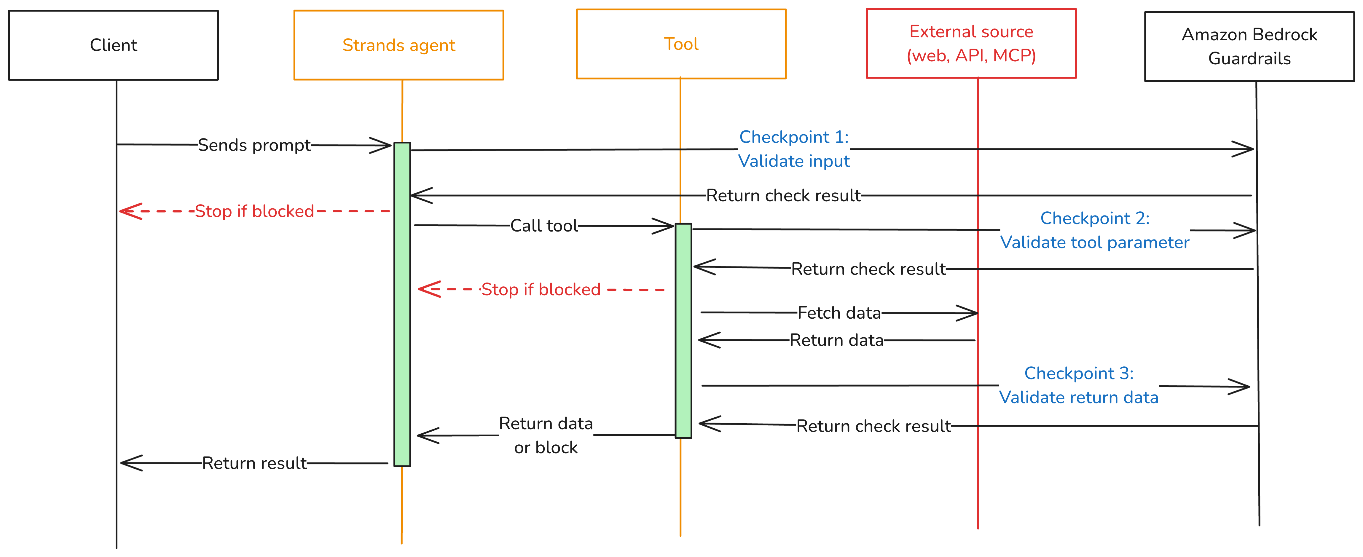
To close these gaps, add three validation checkpoints at each trust boundary where data crosses into or out of your agent as shown in Figure 1.

  • Checkpoint 1: Inbound data validation – Check data before it reaches the model—user input, data from other agents, MCP tool servers, and RAG pipelines. You catch policy-violating or biased content before it enters the model’s context window. In the Strands Agents SDK, you implement this using a BeforeInvocationEvent hook that fires before model inference or tool execution occurs. The hook inspects incoming messages and blocks the request if the content violates policies. The model doesn’t see blocked content.
  • Checkpoint 2: Tool interaction supervision – Before the agent calls a tool, a BeforeToolCallEvent hook checks the parameters it’s about to pass. This is the gap model-level guardrails don’t cover. The model has already decided what to send, but nothing has verified whether that content is safe to act on. If the hook flags the input, the call is canceled before the real-world action occurs.
  • Checkpoint 3: Outbound data validation – Validate results before returning them to the user or passing them to downstream systems. You need this most for tools that ingest external content, like a web search tool fetching web pages from sites outside your control. In Strands, an AfterToolCallEvent hook validates the tool’s return value and replaces it with a block message if the content violates policies.
Figure 1: Three validation checkpoints extend Amazon Bedrock Guardrails from the model boundary to the tool boundary.

Figure 1: Three validation checkpoints extend Amazon Bedrock Guardrails from the model boundary to the tool boundary.

You can adjust the validation intensity of each checkpoint:

  • At Checkpoint 1, use a full Amazon Bedrock guardrail with PII detection, content filtering, and topic enforcement.
  • Checkpoint 2 can be lighter. Configure a separate Amazon Bedrock guardrail with rules tailored to the specific tool being called, or run local checks like regex validation or schema enforcement.
  • For Checkpoint 3, focus on unwanted content detection for tool outputs that return external data.

Mix fast deterministic checks (regex, schema validation, allowlists) with AI-based guardrail evaluations. This keeps latency low.

Implementation

The implementation uses boto3, the AWS SDK for Python, to call the ApplyGuardrail API. The Strands Agents SDK exposes one life-cycle event per checkpoint. Here’s how to implement each one.

Prerequisites

This post assumes you already have a working Strands agent. Your agent should use least-privilege tool access, scoped system prompts, and validated business logic. If you’re starting from scratch, see Strands Agents SDK: A technical deep dive into agent architectures and observability for a step-by-step walk through of building and deploying a Strands agent with Amazon Bedrock Agent Core.

Before implementing the multi-checkpoint approach, you’ will need:

  1. An AWS account with access to Amazon Bedrock
  2. Amazon Bedrock Guardrails configured (see Creating a guardrail)
  3. Python 3.11 or later installed
  4. The Strands Agents SDK installed: pip install strands-agents
  5. AWS credentials configured with permissions for bedrock:ApplyGuardrail and bedrock:InvokeModel
  6. Your guardrail ID and version from the AWS Management Console for Amazon Bedrock (navigate to Guardrails, select your guardrail, and copy the ID)

Create the guardrail validation hook

The GuardrailHook class is a Strands HookProvider. It registers three callbacks, one for each lifecycle event. When Strands triggers an event, the matching callback runs validate_inbound checks user messages, validate_input checks tool parameters before execution, and validate_output checks tool results. All three use the shared _check method, which calls the Amazon Bedrock ApplyGuardrail API.

Create a guardrail_hook.py file and add this implementation. Use the optional tool_names parameter to scope a hook to specific tools, or pass None to apply it everywhere:

import boto3
from strands.hooks import HookProvider, HookRegistry
from strands.hooks.events import (
    BeforeInvocationEvent,
    BeforeToolCallEvent,
    AfterToolCallEvent,
)

class GuardrailHook(HookProvider):

    def __init__(self, guardrail_id, guardrail_version, region_name, tool_names=None):
        self.client = boto3.client("bedrock-runtime", region_name=region_name)
        self.guardrail_id = guardrail_id
        self.guardrail_version = guardrail_version
        self.tool_names = tool_names  # None = apply to all tools

    def register_hooks(self, registry: HookRegistry, **kwargs):
        registry.add_callback(BeforeInvocationEvent, self.validate_inbound)
        registry.add_callback(BeforeToolCallEvent, self.validate_input)
        registry.add_callback(AfterToolCallEvent, self.validate_output)

    def _check(self, content, source="INPUT"):
        """Call Bedrock ApplyGuardrail. Returns True if content is safe."""
        response = self.client.apply_guardrail(
            guardrailIdentifier=self.guardrail_id,
            guardrailVersion=self.guardrail_version,
            source=source,       # "INPUT" applies input policies; "OUTPUT" applies output policies
            content=[{"text": {"text": content}}],
        )
        return response["action"] != "GUARDRAIL_INTERVENED"

    # Checkpoint 1 — BeforeInvocationEvent
    # Validates user input before model inference or tool execution occurs.
    # The model does not see blocked content.
    async def validate_inbound(self, event: BeforeInvocationEvent):
        for msg in reversed(event.messages):
            if msg.get("role") == "user":
                for block in msg.get("content", []):
                    text = block.get("text", "")
                    if text and not self._check(text):
                        event.messages.clear()
                        event.messages.append({
                            "role": "user",
                            "content": [{"text": "Request blocked by safety guardrail."}],
                        })
                        return
                break

    # Checkpoint 2 — BeforeToolCallEvent
    # Validates tool input parameters before the tool executes.
    # Skips tools not in tool_names (if a filter is set).
    async def validate_input(self, event: BeforeToolCallEvent):
        if self.tool_names and event.tool_use.get("name") not in self.tool_names:
            return
        tool_input = event.tool_use.get("input", {})
        for param_value in tool_input.values():
            if isinstance(param_value, str) and not self._check(param_value):
                event.cancel_tool = "This request was blocked by a safety guardrail."
                return

    # Checkpoint 3 — AfterToolCallEvent
    # Validates tool output before it reaches the agent.
    # Skips tools not in tool_names (if a filter is set).
    async def validate_output(self, event: AfterToolCallEvent):
        if self.tool_names and event.tool_use.get("name") not in self.tool_names:
            return
        content_parts = [
            block["text"]
            for block in event.result.get("content", [])
            if "text" in block
        ]
        content = "\n".join(content_parts)
        if content and not self._check(content, source="OUTPUT"):
            event.result = {
                "toolUseId": event.result["toolUseId"],
                "status": "error",
                "content": [{"text": "Content blocked by safety guardrail."}],
            }

Define tools

Strands discovers tools through the @tool decorator. The decorator turns a plain Python function into a tool the model can call, using the function’s docstring and type hints as the tool’s contract. Here are two simple examples used in the registration sections below. A web search tool and a customer data tool:

from strands import tool

@tool
def web_search(query: str) -> str:
    """Search the web and return a result snippet."""
    # Replace with your actual search implementation
    return f"Search results for: {query}"

@tool
def get_customer_data(customer_id: str) -> str:
    """Retrieve customer record by ID."""
    # Replace with your actual data lookup implementation
    return f"Customer record for: {customer_id}"

If you don’t have existing tools, create a tools.py file and copy in the example code above.

Register the hook

Strands activates hooks through the hooks parameter on the Agent constructor. After being registered, the hook’s callbacks run automatically on every matching lifecycle event. No changes are needed in your tools or agent logic. For a single guardrail applied to all tools, create one hook instance and pass it to your agent:

from strands import Agent
from strands.models import BedrockModel
from guardrail_hook import GuardrailHook
from tools import web_search, get_customer_data # Example tools - replace with your tools

# Example model and region selection
model = BedrockModel(
    model_id="us.anthropic.claude-sonnet-4-5",
    region_name="us-east-1",
)

guardrail_hook = GuardrailHook(
    guardrail_id="your-guardrail-id",    # Copy it from the Amazon Bedrock console > Guardrails
    guardrail_version="1",               # Use "DRAFT" for testing
    region_name="us-east-1",             # Region where the guardrails are defined
)

agent = Agent(
    model=model,
    tools=[web_search, get_customer_data], # Example tools
    system_prompt="You are a helpful assistant.", # Example system prompt
    hooks=[guardrail_hook],  # Applied to all tool calls
)

Use different guardrails per tool

Different tools carry different risks. A web search tool fetches external content from untrusted sites and needs strict output filtering. A customer data tool returns internal records and might need PII detection configured differently. The tool_names parameter scopes a hook to specific tools. Strands still runs every registered hook on each event, but hooks skip the call when the tool name doesn’t match. Register one hook per guardrail:

from strands import Agent
from strands.models import BedrockModel
from guardrail_hook import GuardrailHook
from tools import web_search, get_customer_data # Example tools - replace with your tools

# Example model and region selection
model = BedrockModel(
    model_id="us.anthropic.claude-sonnet-4-5",
    region_name="us-east-1",
)
# Strict content filtering and PII detection for web search results
web_search_hook = GuardrailHook(
    guardrail_id="gr-websearch-id",      # Guardrail ID with content filtering + PII detection
    guardrail_version="1",               # Or set to DRAFT
    region_name="us-east-1",             # Change to your region
    tool_names={"web_search"},           # Only applies to the web_search tool
)

# PII detection for customer data — prevents sensitive records from leaking into tool parameters
customer_data_hook = GuardrailHook(
    guardrail_id="gr-customerdata-id",   # Guardrail ID with PII detection
    guardrail_version="1",               # Or set to DRAFT
    region_name="us-east-1",             # Change to your region
    tool_names={"get_customer_data"},    # Only applies to the get_customer_data tool
)

agent = Agent(
    model=model,
    tools=[web_search, get_customer_data],        # Example tools
    system_prompt="You are a helpful assistant.", # Example system prompt
    hooks=[web_search_hook, customer_data_hook],  # Each hook runs only for its assigned tools
)

Each guardrail is configured independently in the Amazon Bedrock console. You can match validation strictness to each tool’s risk level instead of applying one policy across your entire agent.

Test your implementation

Run a quick test with the preceding examples:

  1. Create a project folder and add the following files:
    1. guardrail_hook.py the GuardrailHook class
    2. tools.py the web_search and get_customer_data tool definitions as examples
    3. agent.py the agent setup from the Register the hook section
  2. In agent.py, add a test prompt at the end:
# Send a test prompt
response = agent("Search the web for the latest news on AI security.")
print(response)

  1. Update the guardrail IDs, AWS Region, and model ID in agent.py to match your configuration.
  2. Run the agent from your project folder: python agent.py

The guardrail hook runs at each checkpoint. If the prompt or any tool output is flagged, you’ll see the block message in the response instead of the tool result.

Use the hook across your organization

The GuardrailHook is a standalone HookProvider. Build it once, then attach it to Strands agents by passing it to the hooks parameter. The same hook package can be published as an internal library and consumed by

You can swap guardrail configurations or add checks like regex or schema validation without touching agent or tool code.

Conclusion

Amazon Bedrock Guardrails protects the model boundary, but agents also call tools, consume external data, and return results that never pass through model-level checks. The three validation checkpoints in this post close that gap using Strands Agents SDK lifecycle hooks: BeforeInvocationEvent validates user input, BeforeToolCallEvent validates tool parameters, and AfterToolCallEvent validates tool output. The same GuardrailHook class supports one shared guardrail or different guardrails scoped per tool, and deploys unchanged from local testing to Amazon Bedrock Agent Core Runtime.

To learn more, see:

If you have feedback about this post, submit comments in the Comments section below.


Stephan Traub

Stephan Traub

Stephan is a senior security consultant with AWS Professional Services, where he works closely with customers across different industries. A true technology enthusiast, Stephan is passionate about empowering customers to achieve a robust security posture within their cloud environments and AI workloads. When Stephan isn’t immersed in his AWS work, you can find him on the volleyball court or exploring the world with his family.

How Picnic configured multiple OAuth providers for Amazon MQ

Post Syndicated from Oscar Mapfumo Sibanda original https://aws.amazon.com/blogs/big-data/how-picnic-configured-multiple-oauth-providers-for-amazon-mq/

This post is co-written with Oscar Mapfumo Sibanda from Picnic.

Picnic is an Amsterdam-based tech scale-up that reinvents how people buy food. It isn’t a supermarket with a digital layer but a tech company that happens to deliver groceries. Picnic is engineered in-house: the customer app, the fulfillment platform, the supply chain, and the routing technology that guides a fleet of thousands of electric vehicles through the Netherlands, Germany, and France. Software doesn’t merely support business. Software is a business.

At the center of this system, RabbitMQ is the core component. It’s the communication backbone connecting hundreds of microservices across the entire business lifecycle, from ordering and logistics to delivery and finance. At peak, Picnic’s platform processes close to one million messages per second. At this scale, messaging is no longer only background infrastructure. It becomes part of the company’s operational nervous system. To keep that system highly available, scalable, and resilient as Picnic grows, the company decided to use Amazon MQ as a managed service.

The next challenge was identity. Picnic’s authentication strategy clearly distinguishes between people and services. Operators sign in through Keycloak, the company’s single sign-on provider, while Picnic’s Amazon Elastic Kubernetes Service (Amazon EKS) workloads are adopting AWS Identity and Access Management (IAM) authentication to eliminate static credentials. A single broker therefore must trust two identity providers at once. The Amazon MQ documentation covers configuring OAuth 2.0 with a single provider. This post extends that guidance to a multi-provider setup on the same broker.

In this post, we show how Picnic solved that problem. You will learn how to configure an Amazon MQ for RabbitMQ broker to accept tokens from multiple OAuth 2.0 identity providers, using Keycloak and IAM as the working example. You will also see how to map each provider’s scopes to RabbitMQ permissions and how to roll the change out on a running broker without disrupting connected users.

Background and prerequisites

Amazon MQ for RabbitMQ supports OAuth 2.0 authentication and authorization, where broker users and their permissions are managed by an external identity provider. User authentication and resource permissions for vhosts, exchanges, queues, and topics are centralized through the OAuth 2.0 provider’s scope system.

RabbitMQ’s OAuth 2.0 plugin supports multiple resource servers and audiences, allowing different OAuth 2.0 providers to issue tokens that a single broker can validate. This capability is essential if you operate in multiple environments or have teams registered with separate identity providers.

Prerequisites

To follow along with this post, you need:

  1. An active AWS account.
  2. An Amazon MQ for RabbitMQ broker with OAuth 2.0 configured for at least one identity provider (see Using OAuth 2.0 authentication and authorization for Amazon MQ for RabbitMQ).
  3. A second OAuth 2.0 identity provider configured and operational.
  4. Outbound web identity federation enabled for your AWS account (if using IAM as a provider).
  5. Basic familiarity with RabbitMQ configuration and OAuth 2.0 concepts.
  6. AWS Command Line Interface (AWS CLI) version 2.27 or later (required for the get-web-identity-token command used in the testing section).

Note: The information in this post reflects Amazon MQ for RabbitMQ features and behavior at the time of publication. We recommend checking the Amazon MQ documentation, release notes and best practices before implementation.

Solution architecture

The design rests on a single idea: a RabbitMQ broker can trust more than one identity provider at the same time, and it decides which one to apply per token rather than per broker. RabbitMQ does this by reading the aud (audience) claim of each incoming token and matching it against a configured resource server. Each resource server is bound to one OAuth 2.0 provider, so the audience determines both which signing keys validate the token and which permission rules apply.

Architecture diagram

The following two diagrams show how services and operators authenticate the broker through their respective identity providers.

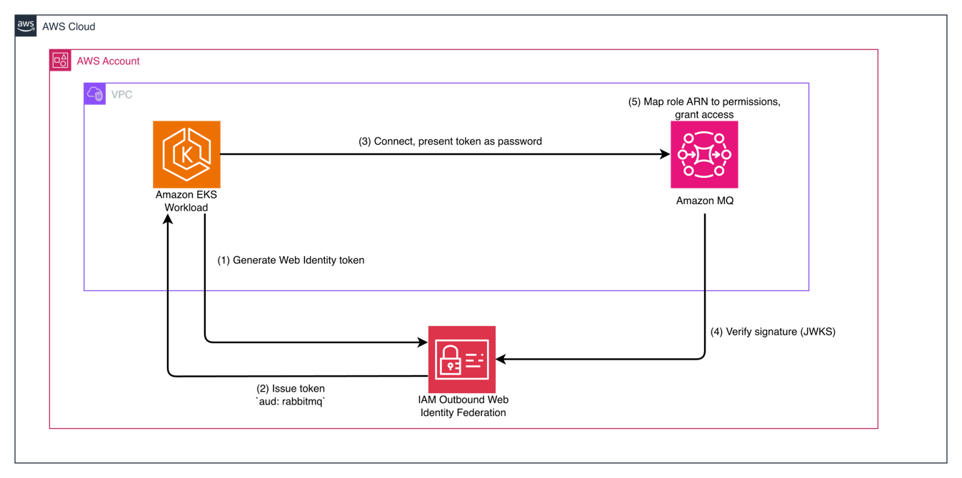
Services authentication flow from an Amazon EKS workload through AWS STS to the Amazon MQ for RabbitMQ broker over AMQPS

Figure 1: Services (IAM) flow

Services authenticate through IAM. An Amazon EKS workload assumes an IAM role and generates a web identity token (1), which AWS Security Token Service (AWS STS) issues with an audience of rabbitmq-iam (2). The workload presents that token as its password when it connects to the broker over Advanced Message Queuing Protocol (AMQPS) on port 5671 (3). The broker selects the matching resource server, verifies the token’s signature against the AWS STS signing keys (4), and maps the role’s Amazon Resource Name (ARN) to the permissions the workload needs (5).

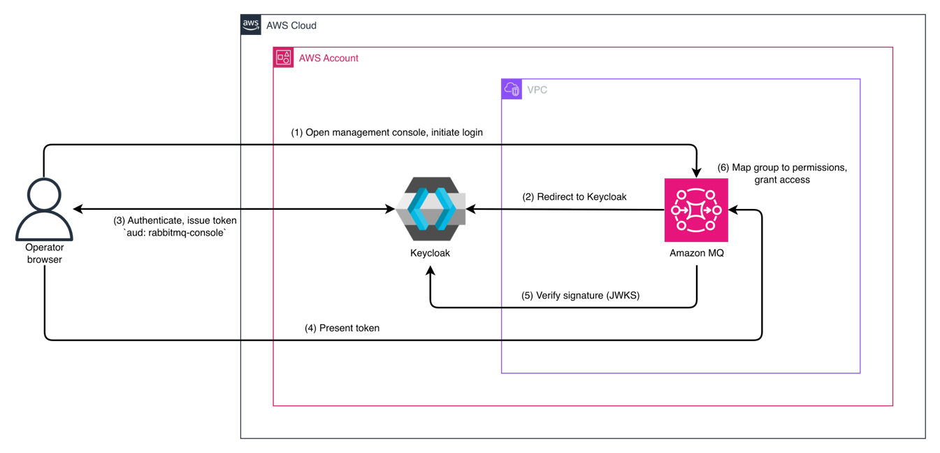
Operators authentication flow from the RabbitMQ management console through Keycloak single sign-on to the broker

Figure 2: Operators (Keycloak) flow

Operators authenticate through Keycloak. An operator opens the RabbitMQ management console and initiates login (1), and the console redirects the browser to Keycloak (2). Keycloak authenticates the operator and issues a token whose audience targets the console resource server, rabbitmq-keycloak (3). The browser presents that token to the broker (4), which verifies the signature against Keycloak’s signing keys (5). The broker then reads the operator’s group membership and grants access (6): the Operator group receives read-only permissions, while the Administrator group receives full control.

Two constraints follow this design. First, audience verification is a single broker-wide setting that applies to every provider at once, so each provider must issue tokens carrying the exact audience its resource server expects. Second, the broker is private, deployed inside an Amazon Virtual Private Cloud (Amazon VPC) with no public exposure. Both providers’ endpoints must be resolvable, either through publicly addressable JSON Web Key Set (JWKS) endpoints or through private networking, because the broker fetches signing keys from those endpoints.

Implementation walkthrough

This walkthrough configures one Amazon MQ for RabbitMQ broker to trust two identity providers: Keycloak for operators and AWS IAM for services. The steps assume you already have a running broker, a Keycloak realm, and outbound web identity federation enabled for your AWS account. All configurations are applied through a RabbitMQ configuration revision using the AWS Command Line Interface (AWS CLI).

Enable OAuth 2.0 on the broker

The first block activates the OAuth 2.0 backend and keeps the internal backend in place. Internal authentication remains active deliberately: Amazon MQ creates an administrator user when the broker is provisioned, and that user is needed for break-glass access.

auth_backends.1 = oauth2
auth_backends.2 = internal
auth_oauth2.verify_aud = true

Setting verify_aud = true tells RabbitMQ to reject any token whose aud claim does not match a configured resource server. This single broker-wide setting governs every provider you add.

Add the first identity provider (Keycloak)

A resource server binds an audience value to a provider and a set of permission rules. The Keycloak resource server uses the id rabbitmq-keycloak, which is the audience the realm must place in its tokens. RabbitMQ reads the operator’s group membership from the group_membership claim and resolves it through scope aliases.

auth_oauth2.resource_servers.1.id = rabbitmq-keycloak
auth_oauth2.resource_servers.1.oauth_provider_id = keycloak
auth_oauth2.resource_servers.1.scope_prefix = rabbitmq.
auth_oauth2.resource_servers.1.additional_scopes_key = group_membership
auth_oauth2.resource_servers.1.preferred_username_claims.1 = email
auth_oauth2.resource_servers.1.scope_aliases.1.alias = Operator
auth_oauth2.resource_servers.1.scope_aliases.1.scope = rabbitmq.read:*/* rabbitmq.write:^$ rabbitmq.configure:^$ rabbitmq.tag:monitoring
auth_oauth2.resource_servers.1.scope_aliases.2.alias = Administrator
auth_oauth2.resource_servers.1.scope_aliases.2.scope = rabbitmq.read:*/* rabbitmq.write:*/* rabbitmq.configure:*/* rabbitmq.tag:administrator

The Operator group is read-only: it can read any resource and view the management UI through the monitoring tag. The Administrator group receives full permissions plus the administrator tag. This role is least privilege by design.

The provider is configured with its issuer and JWKS endpoint:

auth_oauth2.oauth_providers.keycloak.https.hostname_verification = wildcard
auth_oauth2.oauth_providers.keycloak.issuer = https://keycloak.example.com/auth/realms/test
auth_oauth2.oauth_providers.keycloak.jwks_uri = https://keycloak.example.com/auth/realms/test/protocol/openid-connect/certs

To let operators sign in from the management console, expose Keycloak as a management resource:

management.oauth_enabled = true
management.oauth_disable_basic_auth = false
management.oauth_scopes = openid email profile
management.oauth_resource_servers.1.id = rabbitmq-keycloak
management.oauth_resource_servers.1.oauth_client_id = rabbitmq-keycloak
management.oauth_resource_servers.1.label = Keycloak SSO

Add the second identity provider (AWS IAM)

Adding a second provider means adding a second resource server and a second entry under oauth_providers. The IAM resource server uses the id rabbitmq-iam because the audience is set when minting the token.

auth_oauth2.resource_servers.2.id = rabbitmq-iam
auth_oauth2.resource_servers.2.oauth_provider_id = aws_iam
auth_oauth2.resource_servers.2.scope_prefix = rabbitmq/
auth_oauth2.resource_servers.2.additional_scopes_key = sub
auth_oauth2.resource_servers.2.scope_aliases.1.alias = arn:aws:iam::123456789012:role/EKSWorkloadRole
auth_oauth2.resource_servers.2.scope_aliases.1.scope = rabbitmq/read:*/* rabbitmq/write:*/* rabbitmq/configure:*/* rabbitmq/tag:policymaker
auth_oauth2.oauth_providers.aws_iam.https.hostname_verification = wildcard
auth_oauth2.oauth_providers.aws_iam.issuer =
auth_oauth2.oauth_providers.aws_iam.jwks_uri =

The IAM workload receives the policymaker tag. It can publish, consume, and manage policies but does not receive the administrator tag.

Apply the configuration and restart the broker:

CONFIG_ID=$(aws mq describe-broker --broker-id $BROKER_ID \
  --query 'Configurations.Current.Id' --output text)
REVISION=$(aws mq update-configuration --configuration-id $CONFIG_ID \
  --data "$(cat rabbitmq.conf | base64 | tr -d '\n')" \
  --query 'LatestRevision.Revision' --output text)
aws mq update-broker --broker-id $BROKER_ID \
  --configuration Id=$CONFIG_ID,Revision=$REVISION
aws mq reboot-broker --broker-id $BROKER_ID

Note: The base64 command syntax differs between Linux and macOS. The preceding command (cat file | base64 | tr -d '\n') is portable on both operating systems. If running exclusively on Linux, you can also use base64 --wrap=0 rabbitmq.conf. On macOS, the equivalent command is base64 -i rabbitmq.conf.

Testing and validation

Validate each provider independently. For IAM, assume the role and request a token from AWS STS, then present it as the AMQP password:

TOKEN=$(aws sts get-web-identity-token \
  --audience "rabbitmq-iam" \
  --signing-algorithm ES384 \
  --duration-seconds 300 \
  --query 'WebIdentityToken' --output text)
# Username is empty (ignored by the OAuth plugin); the token is passed as the password
curl -u ":$TOKEN" https://<broker-id>.mq.<region>.on.aws/api/overview

Note: The get-web-identity-token API requires outbound web identity federation to be enabled on your AWS account and AWS CLI version 2.27 or later.

A successful response confirms the IAM resource server accepted the token. For Keycloak, open the management console, choose Keycloak SSO, and sign in as an operator.

When a login fails, decode the JSON Web Token (JWT) and check two claims. The aud claim must exactly match a resource server id. With verify_aud = true, a missing or mismatched audience is the most common cause of rejection. If the audience is correct but permissions are missing, verify the scope_prefix is set correctly.

Operational considerations

A few points deserve attention before you run this pattern in production.

  1. Key rotation: When rotating signing keys at a provider, publish the new key in the JWKS endpoint before revoking the old one. The broker caches keys, so overlapping both during the transition window prevents authentication failures while the cache refreshes.
  2. Audience validation: Audience remains the linchpin. With verify_aud enabled, every provider must issue tokens carrying the audience its resource server expects, so confirm this whenever you onboard a new one. Don’t disable audience validation in production. The RabbitMQ OAuth 2.0 plugin does not perform token revocation checks, which makes audience binding a critical control that prevents tokens issued for other services from granting access.
  3. Scope prefix: scope_prefix values are optional. They’re needed only if the tokens don’t follow the default format. RabbitMQ only reads scopes carrying the expected prefix, so a token can authenticate yet grant nothing if the prefix is missing. Map each provider to the least privilege its principals need. For example, prefer narrow scopes like read:orders over blanket read:all to limit the scope of impact if a single provider’s credentials are compromised.
  4. Token lifetime: Because the plugin does not support token revocation, token lifetime is your primary control over leaked credentials. Issue short-lived access tokens and have your client applications refresh them proactively at approximately 75 percent of the token’s lifetime to avoid connection disruptions when a token expires mid-session.
  5. Monitoring: Authentication failures and refused tokens are recorded in the broker’s connection log group in Amazon CloudWatch, which can be reached through the Amazon CloudWatch Logs link on the broker’s page in the Amazon MQ console. Beyond logs, set up CloudWatch alarms on RabbitMQMemUsed, RabbitMQDiskFree, and ConnectionCount. An unexpected spike in failed connections is often the first sign of a token or audience misconfiguration. For unaggregated, per-node visibility, consider enabling the Prometheus metrics endpoint: metrics such as rabbitmq_auth_attempts_failed_total surface OAuth rejections faster than the CloudWatch one-minute polling interval.
  6. Network controls: Enforce defense in depth by restricting broker access using security groups so that only authorized VPCs and IP ranges can reach the AMQPS and management endpoints. This matters especially in an OAuth setup because, once a token has been issued, the broker cannot revoke it before it expires.

Cleanup

To avoid incurring future costs, delete the resources created during this walkthrough if you no longer need them:

  1. Delete Amazon MQ broker and configurations.
  2. Remove test OAuth application registrations from your identity providers.
  3. Delete any IAM roles created for testing.

Conclusion

In this post, we demonstrated how Picnic configured an Amazon MQ for RabbitMQ broker to authenticate tokens from two OAuth 2.0 identity providers: Keycloak for human operators and AWS IAM for machine-to-machine services on a single broker instance. The key mechanism is RabbitMQ’s support for multiple resource servers, where the audience claim in each token determines which provider’s signing keys and permission rules apply.

With this approach, the Picnic team was able to cleanly separate human and machine authentication without the operational overhead of running separate brokers, while retaining fine-grained access control for both token issuers.

This pattern works with any combination of OAuth 2.0 providers and is particularly valuable for organizations looking to consolidate messaging infrastructure while maintaining distinct identity boundaries.

To learn more about Amazon MQ for RabbitMQ and OAuth 2.0 authentication, see Authentication and authorization for Amazon MQ. For a hands-on walkthrough of configuring OAuth 2.0 with Amazon MQ for RabbitMQ, see Using OAuth 2.0 authentication and authorization for Amazon MQ for RabbitMQ. The configuration examples in this post are broker-level settings applied through the Amazon MQ API. No standalone code repository is required.


About the authors

Oscar Mapfumo Sibanda

Oscar Mapfumo Sibanda

Oscar is a Senior Site Reliability Engineer at Picnic Technologies in the Netherlands. He builds infrastructure that supports rapid scaling, empowers engineering teams to move independently, and strengthens the security posture across the organization. Outside of work he paints and takes photographs; he is a technology enthusiast in the pursuit of happiness.

Ayush Kumar

Ayush Kumar

Ayush is a Technical Account Manager at Amazon Web Services based in the Netherlands. He works with enterprise customers to optimize their cloud architectures and accelerate innovation on AWS. You’ll find him experimenting in the kitchen in his spare time.

Amit Singh

Amit Singh

Amit is a Senior Solutions Architect at AWS, working with enterprise retail customers in the Benelux region. He helps customers design cloud-native architectures, navigate complex modernization journeys, and adopt AI/ML capabilities at scale. Outside of work, he enjoys exploring new places and chasing the perfect shot, whether through a camera lens or on a running trail.

Build with geospatial and variant types in Iceberg v3 on AWS Glue 6.0

Post Syndicated from Shoukat Ghouse original https://aws.amazon.com/blogs/big-data/build-with-geospatial-and-variant-types-in-iceberg-v3-on-aws-glue-6-0/

As organizations build data lakes that combine geospatial data, high-frequency event streams, and heterogeneous payloads, the limitations of older table formats become acute. Without a native geospatial type, coordinates require separate float columns (latitude/longitude) with no spatial predicates. Without nanosecond-precision timestamps, sub-microsecond event ordering is lost. Without a variant type, semi-structured data forces a choice between rigid flattening and untyped JSON strings. Each workaround adds complexity, slows queries, and increases maintenance burden.

AWS Glue 6.0, powered by Apache Spark 4.1, removes these workarounds by adding support for Apache Iceberg v3, bringing new column-level capabilities to your data lake tables. These include new data types: native geospatial types (GEOMETRY with spatial predicates, and GEOGRAPHY), nanosecond-precision timestamps, and the VARIANT type for semi-structured data with automatic shredding. Iceberg v3 also adds support for DEFAULT column values. These are table format features. After they’re written, they’re readable by any Iceberg v3-compatible engine that supports these features.

In this post, we build a connected vehicle fleet monitoring pipeline that uses these capabilities in a single Iceberg v3 table. Vehicles emit telemetry events with GPS coordinates (geospatial), sub-microsecond event times (nanosecond), and sensor payloads that vary by vehicle type (variant). We ingest these events, run spatial queries to detect geofence violations, sequence events at nanosecond precision, and extract typed metrics from heterogeneous payloads, all without workarounds, flattening, or external libraries.

Solution overview

A logistics company operates a mixed fleet of delivery vehicles: vans, electric bikes, and delivery robots. Each vehicle type produces telemetry events with a different sensor payload schema. The operations team needs to:

  1. Detect geofence violations: flag vehicles that enter restricted zones (airports, pedestrian areas, private property).
  2. Sequence events precisely: at fleet scale, many events land in the same microsecond window. Nanosecond timestamps give a deterministic order and prevent ties when sequencing or deduplicating events during processing.
  3. Extract metrics from heterogeneous payloads: query battery level from delivery robots, fuel level from vans, and pedal cadence from bikes, all stored in the same column.

We address all three requirements with a single Iceberg v3 table on AWS Glue 6.0. The following data definition language (DDL) shows the table structure. The AWS Glue job we provision in subsequent steps executes this statement.

CREATE TABLE fleet_monitoring_db.vehicle_telemetry (
event_id STRING,
vehicle_id STRING,
vehicle_type STRING DEFAULT 'UNKNOWN',
event_time TIMESTAMP_NTZ(9),
location GEOMETRY(4326),
service_area GEOGRAPHY(4326),
sensor_payload VARIANT,
speed_kmh DOUBLE DEFAULT 0.0,
region STRING DEFAULT 'EMEA'
) USING ICEBERG
TBLPROPERTIES (
'format-version' = '3',
'write.delete.mode' = 'merge-on-read'
)
PARTITIONED BY (days(event_time), vehicle_type)

In the preceding statement, the database is shown as fleet_monitoring_db for readability. The deployed stack creates it as fleet_monitoring_<account-id>.

The following list describes the key columns:

  • event_time TIMESTAMP_NTZ(9): Stores the event timestamp at nanosecond precision.
  • location GEOMETRY(4326): Stores GPS coordinates as native spatial objects using (SRID 4326). You can use predicates like ST_Intersects directly in SQL, replacing hand-coded spatial math on raw latitude/longitude doubles (WGS 84).
  • service_area GEOGRAPHY(4326): Stores geographic coordinates using a spherical (geodesic) model, distinct from GEOMETRY’s planar model. AWS Glue 6.0 writes and reads GEOGRAPHY in Iceberg v3, and the type is portable to any Iceberg v3-compatible engine. Geodesic spatial predicates over GEOGRAPHY are engine-dependent today. In this post we run spatial queries on the GEOMETRY location column, which Glue 6.0 supports natively.
  • sensor_payload VARIANT: Each vehicle type produces a different JSON schema. Vans report fuel and engine metrics, robots report battery and camera status, bikes report cadence and heart rate. All land in this single column without schema unions or separate tables using variant data type.
  • vehicle_type STRING DEFAULT ‘UNKNOWN’ and speed_kmh DOUBLE DEFAULT 0.0: When an ingestion writer omits these fields, Iceberg applies the declared defaults automatically. Useful when multiple producers write to the same table and not all of them populate every column.

The table uses PARTITIONED BY (days(event_time), vehicle_type) so that analytical queries can prune by date range and vehicle type without scanning the full table. 'write.delete.mode' = 'merge-on-read' supports fast row-level corrections (for example, correcting a misreported GPS coordinate) through compact deletion vectors (Roaring Bitmaps) instead of accumulating positional delete files.

In this post, we insert sample data directly to focus on the new Iceberg data types and how to use them together. In production, these events would stream from Amazon Managed Streaming for Apache Kafka (Amazon MSK) into an AWS Glue 6.0 streaming job.

The following diagram illustrates the production architecture for reference:

Architecture diagram showing a vehicle fleet of vans, delivery robots, and electric bikes sending telemetry through Amazon MSK into an AWS account. Within a VPC, a hot path uses AWS Glue 6.0 Spark Real-Time Mode to detect geofence violations and send alerts to a Kafka topic, while a cold path uses a Glue 6.0 micro-batch job to write events into an Apache Iceberg v3 table with GEOMETRY, TIMESTAMP_NTZ(9), VARIANT, and DEFAULT columns. Amazon S3 stores the Iceberg data and the AWS Glue Data Catalog holds metadata. A batch analytics Glue job reads the Iceberg table for geofence detection, nanosecond event sequencing, and per-vehicle-type metric extraction using variant_get

Figure 1: Reference architecture for a fleet telemetry pipeline on AWS Glue 6.0

The architecture processes vehicle telemetry through two paths, with a downstream batch analytics layer:

Hot path (real-time, milliseconds): A Spark Real-Time Mode (RTM) job reads telemetry from Amazon MSK and evaluates geofence violations using spatial predicates like ST_Intersects, routing alerts to a downstream Kafka topic within milliseconds.

Cold path (near-real-time, seconds): A micro-batch job reads the same MSK topic and writes events into an Iceberg v3 table, converting payloads to GEOMETRY, TIMESTAMP_NTZ(9), and VARIANT columns with DEFAULT values applied.

Batch analytics: An AWS Glue job reads the Iceberg v3 table to run batch analytics on geofence detection, nanosecond event sequencing, and per-vehicle-type metric extraction.

Prerequisites

To follow along, you need:

  • An AWS account and an AWS Region where AWS Glue 6.0 is available.
  • An AWS Identity and Access Management (IAM) role with permissions to deploy AWS CloudFormation stacks and create resources including AWS Glue, Amazon Simple Storage Service (Amazon S3), and Amazon CloudWatch Logs.

Deploy the CloudFormation stack

We provide an AWS CloudFormation template that provisions all the resources needed for this walkthrough.

The stack provisions the following resources:

  • An Amazon S3 bucket for Iceberg table storage.
  • An IAM role with permissions for AWS Glue, Amazon S3, and Amazon CloudWatch Logs.
  • An AWS Glue database (fleet_monitoring_<account-id>).
  • An AWS Glue job fleet-telemetry-ingest-<account-id> (PySpark): creates the Iceberg v3 table vehicle_telemetry described earlier and inserts sample telemetry from three vehicle types.
  • An AWS Glue job fleet-telemetry-queries-<account-id> (PySpark): demonstrates geofence detection, nanosecond sequencing, variant extraction, and default values.

Deploy the CloudFormation stack:

  1. Download the CloudFormation template from the GitHub repository.
  2. Sign in to the AWS CloudFormation console.
  3. Choose Create stack, With new resources, Upload a template file, and upload the downloaded template.
  4. Acknowledge the IAM capabilities and choose Create stack.

Stack creation takes approximately 2–5 minutes. No parameters are required.

After the stack completes, navigate to the AWS Glue console and run the jobs in this order:

  1. Run fleet-telemetry-ingest-<account-id>. This job creates the Iceberg v3 table and inserts sample data (approximately 2 minutes).
  2. After it succeeds, run fleet-telemetry-queries-<account-id>. This job executes all demonstration queries (approximately 2 minutes).

The following sections describe each job in detail.

Job 1: Ingest sample telemetry data

The ingestion job creates the Iceberg v3 table described earlier and inserts four sample telemetry events: one for each of the three vehicle types (van, robot, bike), plus one with omitted fields to demonstrate DEFAULT values. You can view the complete script in the GitHub repository. Note that the geospatial types require one additional Spark configuration (spark.sql.geospatial.enabled=true), which is already set in the job’s --conf argument by the CloudFormation template. All other types work with no extra configuration.

The following are the key snippets from the script:

Van telemetry: GPS coordinates with engine metrics and route information:

spark.sql(f"""
INSERT INTO {TABLE} VALUES (
'EVT-001', 'VAN-042', 'VAN',
CAST('2026-07-28 09:15:30.123456789' AS TIMESTAMP_NTZ(9)),
ST_SetSrid(ST_GeomFromWKB(X'0101000000E17A14AE47E1C0BF1F85EB51B84E4940'), 4326),
ST_SetSrid(ST_GeogFromWKB(X'0101000000E17A14AE47E1C0BF1F85EB51B84E4940'), 4326),
PARSE_JSON('{{"fuel_pct": 0.72, "cargo_kg": 450, "door_open": false,
"engine": {{"rpm": 2100, "temp_c": 88.5}},
"route": {{"stops_remaining": 4, "eta_minutes": 35}}}}'),
35.2, 'EMEA'
)
""")

Delivery robot telemetry: Same table, completely different sensor schema (battery, cameras, navigation):

spark.sql(f"""
INSERT INTO {TABLE} VALUES (
'EVT-002', 'ROB-117', 'ROBOT',
CAST('2026-07-28 09:15:30.123456790' AS TIMESTAMP_NTZ(9)),
ST_SetSrid(ST_GeomFromWKB(X'01010000000000000000001040000000000000F03F'), 4326),
ST_SetSrid(ST_GeogFromWKB(X'01010000000000000000001040000000000000F03F'), 4326),
PARSE_JSON('{{"battery_pct": 0.62, "obstacle_distance_m": 2.8,
"navigation_mode": "autonomous",
"cameras": {{"front": "active", "rear": "recording"}}}}'),
48.0, 'EMEA'
)
""")

Note: EVT-001 and EVT-002 are exactly 1 nanosecond apart (.123456789 vs .123456790). Without TIMESTAMP_NTZ(9), both would round to the same microsecond and be indistinguishable.

Default values test: Event inserted with vehicle_type, speed_kmh, and region omitted:

spark.sql(f"""
INSERT INTO {TABLE}
(event_id, vehicle_id, event_time, location, service_area, sensor_payload)
VALUES (
'EVT-004', 'UNK-999',
CAST('2026-07-28 10:00:00.000000000' AS TIMESTAMP_NTZ(9)),
ST_SetSrid(ST_GeomFromWKB(X'0101000000000000000000F03F000000000000F03F'), 4326),
ST_SetSrid(ST_GeogFromWKB(X'0101000000000000000000F03F000000000000F03F'), 4326),
PARSE_JSON('{{"status": "initializing"}}')
)
""")

The omitted columns automatically receive their DEFAULT values: vehicle_type = 'UNKNOWN', speed_kmh = 0.0, region = 'EMEA'.

Job 2: Query the data

The query job demonstrates all four data types working together. After the job succeeds, select the run in the AWS Glue console and choose Output logs to see the results.

The following sections walk through the key queries from the job and the results of each.

Geofence detection with ST_Intersects

The job defines a polygon and finds all vehicles inside it:

POLY = "010300...."
SELECT event_id, vehicle_id, vehicle_type, speed_kmh
FROM fleet_monitoring_db.vehicle_telemetry
WHERE ST_Intersects(
location,ST_SetSrid(ST_GeomFromWKB(X'{POLY}'), 4326)
)
ORDER BY event_id

The polygon covers coordinates (0,0)-(5,0)-(5,2)-(0,2). Three vehicles are inside (ROBOT at (4,1), BIKE at (3,1), UNKNOWN at (1,1)). The VAN at (-0.1278, 51.5074) is outside.

Query results listing the ROBOT, BIKE, and UNKNOWN vehicles inside the geofence polygon, with the VAN excluded

Figure 2: Geofence query results showing the three vehicles inside the polygon

Nanosecond event sequencing

Order events by their sub-microsecond timestamps:

SELECT event_id, vehicle_id, CAST(event_time AS STRING) AS precise_time
FROM fleet_monitoring_db.vehicle_telemetry
WHERE event_id IN ('EVT-001', 'EVT-002', 'EVT-003')
ORDER BY event_time ASC

EVT-001 and EVT-002 are correctly distinguished and ordered despite being only 1 nanosecond apart. With standard TIMESTAMP_NTZ (microsecond precision), both would show .123456 and their relative order would be undefined.

Query results showing EVT-001 and EVT-002 ordered by nanosecond-precision timestamps one nanosecond apart

Figure 3: Nanosecond-precision ordering distinguishing two events one nanosecond apart

Variant extraction with variant_get

Different sensor schemas per vehicle type, all extracted with variant_get:

SELECT vehicle_id, vehicle_type,
CASE vehicle_type
WHEN 'VAN' THEN variant_get(sensor_payload, '$.fuel_pct', 'DOUBLE')
WHEN 'ROBOT' THEN variant_get(sensor_payload, '$.battery_pct', 'DOUBLE')
WHEN 'BIKE' THEN variant_get(sensor_payload, '$.battery_pct', 'DOUBLE')
ELSE NULL
END AS energy_level,
variant_get(sensor_payload, '$.engine.temp_c', 'DOUBLE') AS engine_temp,
variant_get(sensor_payload, '$.cameras.front', 'STRING') AS front_cam,
variant_get(sensor_payload, '$.deliveries.completed', 'INT') AS deliveries_done
FROM fleet_monitoring_db.vehicle_telemetry
WHERE vehicle_type != 'UNKNOWN'
ORDER BY vehicle_id
Query results showing variant_get extracting energy level, engine temperature, and camera status for each vehicle type

Figure 4: Variant extraction returning typed values from heterogeneous sensor payloads

variant_get takes three arguments: the column, a dot-path expression, and the expected return type. It supports arbitrary nesting depth. $.engine.temp_c reaches two levels deep, $.deliveries.completed reaches into a different structure entirely. When a path doesn’t exist in a particular row’s payload, it returns NULL.

Default values

Confirm that omitted columns received their defaults:

SELECT event_id, vehicle_type, speed_kmh, region
FROM fleet_monitoring_db.vehicle_telemetry
WHERE event_id = 'EVT-004'
Query results showing event EVT-004 with the default values UNKNOWN, 0.0, and EMEA applied

Figure 5: Default column values applied to the event inserted with omitted fields

EVT-004 was inserted without vehicle_type, speed_kmh, or region. The declared defaults were applied automatically.

Combined query: Combining spatial, temporal, and variant operations

The following query runs a geospatial predicate, nanosecond ordering, and variant extraction in a single SELECT statement:

SELECT vehicle_id, vehicle_type,
CAST(event_time AS STRING) AS precise_time,
CASE vehicle_type
WHEN 'VAN' THEN variant_get(sensor_payload, '$.fuel_pct', 'DOUBLE')
WHEN 'ROBOT' THEN variant_get(sensor_payload, '$.battery_pct', 'DOUBLE')
WHEN 'BIKE' THEN variant_get(sensor_payload, '$.battery_pct', 'DOUBLE')
ELSE NULL
END AS energy_level,
speed_kmh
FROM fleet_monitoring_db.vehicle_telemetry
WHERE ST_Intersects(location, ST_SetSrid(ST_GeomFromWKB(X'0103000000...'), 4326))
ORDER BY event_time ASC
Query results combining spatial filtering, nanosecond ordering, and variant extraction in a single query

Figure 6: Combined query results over a single Iceberg v3 table

This single query combines a spatial predicate, nanosecond ordering, and variant extraction over one table, with no external libraries, pre-processing, or joins to separate geometry or payload tables.

Clean up

To avoid ongoing charges from the AWS Glue jobs and Amazon S3 storage, delete the CloudFormation stack when you’re done:

  1. Open the AWS CloudFormation console.
  2. Select the stack you deployed earlier and choose Delete.

Conclusion

In this post, we stored and analyzed geospatial coordinates, nanosecond timestamps, and heterogeneous sensor payloads in a single Iceberg v3 table on AWS Glue 6.0, with sensible defaults applied automatically, no external libraries, and no schema flattening.

  • GEOMETRY columns replace latitude/longitude doubles and support native spatial predicates like ST_Intersects for geofence detection. GEOGRAPHY is stored natively.
  • TIMESTAMP_NTZ(9) preserves full nanosecond precision for event sequencing where microsecond resolution is insufficient.
  • VARIANT stores heterogeneous payloads (different schema per vehicle type) in one column with typed extraction through variant_get.
  • DEFAULT values keep field population consistent across multiple ingestion writers without duplicating logic.

All capabilities require Iceberg format-version 3. Geospatial requires one additional configuration (spark.sql.geospatial.enabled=true). Nanosecond timestamps, Variant, and DEFAULT values work with no extra configuration.

These capabilities apply wherever schemas vary by source (IoT fleets, multi-tenant software as a service (SaaS), event-driven architectures), timestamps need sub-microsecond precision (trading, sensor fusion, autonomous systems), or spatial operations replace coordinate workarounds (logistics, real estate, delivery networks).

For more information, see the AWS launch announcement (launch URL to be added before publishing), the AWS Glue documentation, and the Apache Iceberg v3 specification. AWS Glue 6.0 includes additional capabilities such as Spark Real-Time Mode and Spark Declarative Pipelines, which we cover in separate posts.


About the authors

Shoukat Ghouse

Shoukat Ghouse

Shoukat is a Senior Specialist Solutions Architect for Big Data, Analytics, and Data Governance at Amazon Web Services (AWS). He partners with enterprise and financial services customers across EMEA to design and scale production-grade data lakehouse platforms on Apache Spark, Apache Iceberg, AWS Glue, Amazon EMR, and Amazon SageMaker Unified Studio. His focus spans distributed data processing, fine-grained data governance, and helping organizations build AI-ready data foundations that power analytics and machine learning at scale.

Shrey Malpani

Shrey Malpani

Shrey is a Senior Product Manager Technical at Amazon Web Services (AWS), where he works at the intersection of distributed data processing and data integration. He is focused on building and scaling data integration and data management capabilities across services like AWS Glue, Amazon EMR, and Amazon Redshift that help customers build AI-ready data platforms for their analytics and machine learning workflows.

Kartik

Kartik

Kartik is a Software Development Manager on the AWS Glue team. His team builds generative AI features for the Data Integration and distributed system for data integration.

Creating and testing an End User Messaging RCS agent with AWS CLI

Post Syndicated from Bruno Giorgini original https://aws.amazon.com/blogs/messaging-and-targeting/creating-and-testing-an-end-user-messaging-rcs-agent-with-aws-cli/

A step-by-step walkthrough for setting up a Rich Communication Services (RCS) test agent, from brand assets to verified inbound messaging.

If you’re still sending plain SMS, you’re leaving a significant experience gap on the table. SMS gives you 160 characters of unformatted text, no branding, and zero confirmation that your message was even read. Rich Communication Services (RCS) changes that entirely. It delivers branded carousels, read receipts, typing indicators, high-resolution images, and verified sender identity, all through the native messaging app your customers already use. No app download required, no new account to create.

Compared to over-the-top (OTT) platforms like WhatsApp or iMessage for Business, RCS doesn’t fragment your audience. It works on an Android’s default messaging app with RCS enabled or an iPhone on iOS 18 or later, which means you reach users where they already are. You are not limited to the ones who happen to have a specific app installed. And compared to building a custom in-app messaging experience, RCS requires no SDK, no UI work, and no convincing users to enable notifications.

With AWS End User Messaging, standing up an RCS agent is surprisingly fast. You configure your brand assets, submit a registration, and within minutes you have a test agent sending branded messages through production APIs. This is real infrastructure, not a sandbox. That means you can prototype, validate your integration, and show stakeholders a working demo before committing to a full build.

This post walks through the entire process of creating an RCS test agent using only the AWS Command Line Interface (AWS CLI). Using the CLI means every step is a repeatable, scriptable command. Need to spin up another agent in a different account or Region? Run the same script and you’re done in minutes. By the end, you will have a working agent that can send branded messages to verified testers and receive inbound messages with automatic responses.

What you will build

In this walkthrough, you will:

  1. Create an RCS agent and configure its brand identity (logo, banner, accent color).
  2. Submit a test registration for automated approval.
  3. Add a verified tester device.
  4. Send your first branded RCS message.
  5. Configure and verify inbound messaging with an automatic keyword response.

Prerequisites

Before you begin, confirm you have:

  • An AWS account with access to AWS End User Messaging (Amazon Pinpoint SMS and Voice v2 API)
  • AWS CLI v2.35.12 or later installed and configured with credentials that have pinpoint-sms-voice-v2:* permissions. Version 2.35.12 adds the send-rcs-message command, which you will need for rich media messages (rich cards, carousels, and suggestion chips) beyond this walkthrough. For production deployments, scope the IAM policy down to only the specific actions your application requires. The pinpoint-sms-voice-v2:* scope is convenient for testing but broader than necessary.
  • rsvg-convert for generating brand asset images from SVG (install with brew install librsvg on macOS)
  • A test phone that supports RCS messaging.

Verify your setup:

# Confirm AWS credentials are working
aws sts get-caller-identity
# Verify EUM access
aws pinpoint-sms-voice-v2 describe-spend-limits --region us-east-1
# Confirm rsvg-convert is installed
which rsvg-convert

If you use a named AWS CLI profile, append --profile <your-profile> to every AWS command in this walkthrough.

Step 1: Create the RCS agent

The first step is to create an empty RCS agent container. The agent’s display name and branding come from the registration you will configure in Step 2.

aws pinpoint-sms-voice-v2 create-rcs-agent \
  --region us-east-1

Expected output:

{
  "RcsAgentArn": "arn:aws:sms-voice:us-east-1:123456789012:rcs-agent/rcs-a1b2c3d4e5f6a1b2c3d4e5f6a1b2c3d4",
  "RcsAgentId": "rcs-a1b2c3d4e5f6a1b2c3d4e5f6a1b2c3d4",
  "Status": "CREATED",
  "DeletionProtectionEnabled": false,
  "CreatedTimestamp": "2026-07-15T10:00:01.000000-07:00"
}

Save the RcsAgentId and RcsAgentArn values. You will use them throughout this walkthrough.

Next, enable deletion protection to prevent accidental removal. This is especially important once carrier approvals are in place, since re-creating an agent requires a new registration and approval cycle:

aws pinpoint-sms-voice-v2 update-rcs-agent \
  --rcs-agent-id rcs-a1b2c3d4e5f6a1b2c3d4e5f6a1b2c3d4 \
  --deletion-protection-enabled \
  --region us-east-1

Step 2: Generate brand assets

Your RCS agent needs a logo (224×224 px, must be under 50 KB as PNG) and a banner (1440×448 px, must be under 200 KB as PNG). Both must be JPEG or PNG format. You can use your own designs as long as they meet these dimension and size requirements. In this example, we generate them as SVGs and convert to PNG.

Create the logo SVG

Create a file named brand-assets/logo.svg:

<svg xmlns="http://www.w3.org/2000/svg" width="224" height="224" viewBox="0 0 224 224"><defs><linearGradient id="bg" x1="0%" y1="0%" x2="100%" y2="100%"><stop offset="0%" style="stop-color:#0D47A1"/><stop offset="100%" style="stop-color:#1565C0"/></linearGradient></defs><rect width="224" height="224" rx="40" fill="url(#bg)"/><g transform="translate(112,90)"><path d="M-48,-36 L48,-36 C54,-36 58,-32 58,-26 L58,16 C58,22 54,26 48,26             L10,26 L0,42 L-10,26 L-48,26 C-54,26 -58,22 -58,16 L-58,-26             C-58,-32 -54,-36 -48,-36 Z" fill="white" opacity="0.95"/><path d="M-20,-12 C-14,-20 14,-20 20,-12" stroke="#0D47A1" stroke-width="4" fill="none" stroke-linecap="round"/><path d="M-14,-2 C-9,-8 9,-8 14,-2" stroke="#0D47A1" stroke-width="4" fill="none" stroke-linecap="round"/><circle cx="0" cy="6" r="4" fill="#0D47A1"/></g><text x="112" y="168" text-anchor="middle" font-family="Arial, Helvetica, sans-serif" font-size="16" font-weight="bold" fill="white">AWS EUM</text><text x="112" y="188" text-anchor="middle" font-family="Arial, Helvetica, sans-serif" font-size="12" fill="white" opacity="0.85">DEMO</text></svg>

Create the banner SVG

Create a file named brand-assets/banner.svg:

<svg xmlns="http://www.w3.org/2000/svg" width="1440" height="448" viewBox="0 0 1440 448"><defs><linearGradient id="bannerBg" x1="0%" y1="0%" x2="100%" y2="100%"><stop offset="0%" style="stop-color:#0D47A1"/><stop offset="50%" style="stop-color:#1565C0"/><stop offset="100%" style="stop-color:#0D47A1"/></linearGradient></defs><rect width="1440" height="448" fill="url(#bannerBg)"/><circle cx="200" cy="224" r="300" fill="white" opacity="0.03"/><circle cx="1300" cy="100" r="250" fill="white" opacity="0.04"/><text x="720" y="190" text-anchor="middle" font-family="Arial, Helvetica, sans-serif" font-size="56" font-weight="bold" fill="white">    AWS End User Messaging  </text><text x="720" y="250" text-anchor="middle" font-family="Arial, Helvetica, sans-serif" font-size="48" font-weight="bold" fill="white" opacity="0.9">    Demo  </text><text x="720" y="320" text-anchor="middle" font-family="Arial, Helvetica, sans-serif" font-size="24" fill="white" opacity="0.7">    Rich messaging experiences, powered by AWS  </text></svg>

Convert to PNG

rsvg-convert -w 224 -h 224 brand-assets/logo.svg -o brand-assets/logo.png
rsvg-convert -w 1440 -h 448 brand-assets/banner.svg -o brand-assets/banner.png

Verify the file sizes. The logo must be under 50 KB and the banner under 200 KB:

ls -la brand-assets/*.png
# logo.png   ~9 KB
# banner.png ~79 KB

Step 3: Create and configure the registration

RCS agents require a registration that contains all brand details. For testing, use the TEST_RCS_LAUNCH_REGISTRATION type.

Create the registration

aws pinpoint-sms-voice-v2 create-registration \
  --registration-type TEST_RCS_LAUNCH_REGISTRATION \
  --region us-east-1

Expected output:

{
  "RegistrationId": "registration-a1b2c3d4e5f6a1b2c3d4e5f6a1b2c3d4",
  "RegistrationType": "TEST_RCS_LAUNCH_REGISTRATION",
  "RegistrationStatus": "CREATED",
  "CurrentVersionNumber": 1
}

Save the RegistrationId.

aws pinpoint-sms-voice-v2 create-registration-association \
  --registration-id registration-a1b2c3d4e5f6a1b2c3d4e5f6a1b2c3d4 \
  --resource-id rcs-a1b2c3d4e5f6a1b2c3d4e5f6a1b2c3d4 \
  --region us-east-1

Upload brand assets

Upload the logo and banner as registration attachments. Note that --attachment-body and --attachment-url cannot be used together. Use --attachment-body with the fileb:// prefix:

# Upload logo
aws pinpoint-sms-voice-v2 create-registration-attachment \
  --attachment-body fileb://brand-assets/logo.png \
  --region us-east-1
# Save: RegistrationAttachmentId (e.g., attachment-1111aaaa2222bbbb3333cccc4444dddd)
# Upload banner
aws pinpoint-sms-voice-v2 create-registration-attachment \
  --attachment-body fileb://brand-assets/banner.png \
  --region us-east-1
# Save: RegistrationAttachmentId (e.g., attachment-5555eeee6666ffff7777aaaa8888bbbb)

Set registration fields

The registration has 23 fields. Each field has a specific type that determines which CLI parameter to use:

Field type CLI parameter Example
TEXT --text-value --text-value "My Brand"
SELECT --select-choices --select-choices "MULTI_USE"
ATTACHMENT --registration-attachment-id --registration-attachment-id "attachment-abc123"

Do not use --field-values. That parameter does not exist in this CLI.

Set all the TEXT fields:

REG_ID="registration-a1b2c3d4e5f6a1b2c3d4e5f6a1b2c3d4"
REGION="us-east-1"

aws pinpoint-sms-voice-v2 put-registration-field-value \
  --registration-id $REG_ID \
  --field-path "agentDetails.brandName" \
  --text-value "AWS End User Messaging Demo" \
  --region $REGION

aws pinpoint-sms-voice-v2 put-registration-field-value \
  --registration-id $REG_ID \
  --field-path "agentDetails.senderDisplayName" \
  --text-value "AWS End User Messaging Demo" \
  --region $REGION

aws pinpoint-sms-voice-v2 put-registration-field-value \
  --registration-id $REG_ID \
  --field-path "agentDetails.agentDescription" \
  --text-value "Experience the power of rich messaging with AWS End User Messaging" \
  --region $REGION

aws pinpoint-sms-voice-v2 put-registration-field-value \
  --registration-id $REG_ID \
  --field-path "agentDetails.accentColor" \
  --text-value "#0D47A1" \
  --region $REGION

aws pinpoint-sms-voice-v2 put-registration-field-value \
  --registration-id $REG_ID \
  --field-path "agentDetails.contactPhoneNumber" \
  --text-value "+12065550100" \
  --region $REGION

aws pinpoint-sms-voice-v2 put-registration-field-value \
  --registration-id $REG_ID \
  --field-path "agentDetails.contactPhoneLabel" \
  --text-value "Call Us" \
  --region $REGION

aws pinpoint-sms-voice-v2 put-registration-field-value \
  --registration-id $REG_ID \
  --field-path "agentDetails.contactEmailAddress" \
  --text-value "[email protected]" \
  --region $REGION

aws pinpoint-sms-voice-v2 put-registration-field-value \
  --registration-id $REG_ID \
  --field-path "agentDetails.contactEmailLabel" \
  --text-value "Email Us" \
  --region $REGION

aws pinpoint-sms-voice-v2 put-registration-field-value \
  --registration-id $REG_ID \
  --field-path "agentDetails.contactWebsite" \
  --text-value "https://www.example.com" \
  --region $REGION

aws pinpoint-sms-voice-v2 put-registration-field-value \
  --registration-id $REG_ID \
  --field-path "agentDetails.contactWebsiteLabel" \
  --text-value "Visit Website" \
  --region $REGION

aws pinpoint-sms-voice-v2 put-registration-field-value \
  --registration-id $REG_ID \
  --field-path "agentDetails.privacyPolicyUrl" \
  --text-value "https://www.example.com/privacy" \
  --region $REGION

aws pinpoint-sms-voice-v2 put-registration-field-value \
  --registration-id $REG_ID \
  --field-path "agentDetails.privacyPolicyLabel" \
  --text-value "Privacy Policy" \
  --region $REGION

aws pinpoint-sms-voice-v2 put-registration-field-value \
  --registration-id $REG_ID \
  --field-path "agentDetails.termsAndConditionsUrl" \
  --text-value "https://www.example.com/terms" \
  --region $REGION

aws pinpoint-sms-voice-v2 put-registration-field-value \
  --registration-id $REG_ID \
  --field-path "agentDetails.termsAndConditionsLabel" \
  --text-value "Terms and Conditions" \
  --region $REGION

aws pinpoint-sms-voice-v2 put-registration-field-value \
  --registration-id $REG_ID \
  --field-path "agentDetails.serviceName" \
  --text-value "AWS End User Messaging Demo RCS Agent" \
  --region $REGION

aws pinpoint-sms-voice-v2 put-registration-field-value \
  --registration-id $REG_ID \
  --field-path "agentDetails.monthlyRcsVolume" \
  --text-value "1000" \
  --region $REGION

aws pinpoint-sms-voice-v2 put-registration-field-value \
  --registration-id $REG_ID \
  --field-path "complianceKeywords.helpResponse" \
  --text-value "Reply STOP to opt out. For help, contact [email protected]" \
  --region $REGION

aws pinpoint-sms-voice-v2 put-registration-field-value \
  --registration-id $REG_ID \
  --field-path "complianceKeywords.stopResponse" \
  --text-value "You have been unsubscribed. No more messages will be sent." \
  --region $REGION

Set the SELECT fields. These use --select-choices instead of --text-value:

aws pinpoint-sms-voice-v2 put-registration-field-value \
  --registration-id $REG_ID \
  --field-path "agentDetails.useCase" \
  --select-choices "MULTI_USE" \
  --region $REGION

aws pinpoint-sms-voice-v2 put-registration-field-value \
  --registration-id $REG_ID \
  --field-path "agentDetails.billingCategory" \
  --select-choices "CONVERSATIONAL" \
  --region $REGION

aws pinpoint-sms-voice-v2 put-registration-field-value \
  --registration-id $REG_ID \
  --field-path "agentDetails.averageMonthlyRcsFrequency" \
  --select-choices "10" \
  --region $REGION

Set the ATTACHMENT fields. These use --registration-attachment-id:

aws pinpoint-sms-voice-v2 put-registration-field-value \
  --registration-id $REG_ID \
  --field-path "agentDetails.logoImage" \
  --registration-attachment-id "attachment-1111aaaa2222bbbb3333cccc4444dddd" \
  --region $REGION

aws pinpoint-sms-voice-v2 put-registration-field-value \
  --registration-id $REG_ID \
  --field-path "agentDetails.bannerImage" \
  --registration-attachment-id "attachment-5555eeee6666ffff7777aaaa8888bbbb" \
  --region $REGION

A note on accent color

The accent color must meet a 4.5:1 contrast ratio against white. This is the WCAG AA accessibility standard, enforced to make sure the text is readable for users with visual impairments. Colors with an HSL lightness value above ~45% will typically fail this threshold and be rejected with ACCENT_COLOR_CONTRAST_INSUFFICIENT. Safe choices include #0D47A1 (blue), #1B5E20 (green), #BF360C (orange), #B71C1C (red), and #4A148C (purple). If you are using a custom brand color, verify it passes before submitting using the WebAIM Contrast Checker.

Submit the registration

aws pinpoint-sms-voice-v2 submit-registration-version \
  --registration-id $REG_ID \
  --region $REGION

Expected output:

{
  "RegistrationId": "registration-a1b2c3d4e5f6a1b2c3d4e5f6a1b2c3d4",
  "VersionNumber": 1,
  "RegistrationVersionStatus": "SUBMITTED"
}

Step 4: Wait for approval

Poll the registration and agent status. Test registrations typically complete within a few minutes.

# Check registration status
aws pinpoint-sms-voice-v2 describe-registrations \
  --registration-ids $REG_ID \
  --query 'Registrations[0].{Status:RegistrationStatus,Version:CurrentVersionNumber}' \
  --region $REGION

# Check agent status
aws pinpoint-sms-voice-v2 describe-rcs-agents \
  --query "RcsAgents[?RcsAgentId=='rcs-a1b2c3d4e5f6a1b2c3d4e5f6a1b2c3d4'].{Status:Status,TestingStatus:TestingAgent.Status}" \
  --region $REGION

You will see the status progress through these stages:

Registration status Agent status Testing status Meaning
SUBMITTED PENDING PENDING Under review
REVIEWING PENDING PENDING Automated checks in progress
COMPLETE TESTING ACTIVE Ready to use

Wait until TestingAgent.Status shows ACTIVE before proceeding.

NOTE: If the registration returns REQUIRES_UPDATES, run describe-registration-field-values to find fields with a DeniedReason. Create a new registration version with create-registration-version, re-populate all 23 fields (new versions do not inherit values), fix the issue, and re-submit.

Step 5: Add a verified tester

Wait at least 120 seconds after agent creation before adding testers. Then register your test device:

aws pinpoint-sms-voice-v2 create-verified-destination-number \
  --destination-phone-number +12065550199 \
  --rcs-agent-id rcs-a1b2c3d4e5f6a1b2c3d4e5f6a1b2c3d4 \
  --region $REGION

You will receive a tester invitation on your phone within 2 to 20 minutes from “RBM Tester Management.” On iPhone, check the Unknown Senders folder. Tap “Make me a tester” to accept.

After accepting, verify the status:

aws pinpoint-sms-voice-v2 describe-verified-destination-numbers \
  --filters Name=rcs-agent-id,Values=rcs-a1b2c3d4e5f6a1b2c3d4e5f6a1b2c3d4 \
  --region $REGION \
  --query 'VerifiedDestinationNumbers[].{Phone:DestinationPhoneNumber,Status:Status}'

Expected output once accepted:

[
  {
    "Phone": "+12065550199",
    "Status": "VERIFIED"
  }
]

Step 6: Send your first RCS message

Before sending, check for potential blockers.

Check the protect configuration

Verify that the US is not blocked in your account’s default protect configuration:

# List protect configurations
aws pinpoint-sms-voice-v2 describe-protect-configurations --region $REGION

# Check US status on the default (account-default) protect configuration
aws pinpoint-sms-voice-v2 get-protect-configuration-country-rule-set \
  --protect-configuration-id <your-protect-config-id> \
  --number-capability SMS \
  --query 'CountryRuleSet.US' \
  --region $REGION

If the US status is BLOCK, update it to ALLOW:

aws pinpoint-sms-voice-v2 update-protect-configuration-country-rule-set \
  --protect-configuration-id <your-protect-config-id> \
  --country-rule-set-updates '{"US":{"ProtectStatus":"ALLOW"}}' \
  --number-capability SMS \
  --region $REGION

Check the opt-out list

aws pinpoint-sms-voice-v2 describe-opted-out-numbers \
  --opt-out-list-name Default \
  --region $REGION

If your test number appears in the list, remove it:

aws pinpoint-sms-voice-v2 delete-opted-out-number \
  --opt-out-list-name Default \
  --opted-out-number +12065550199 \
  --region $REGION

Now, send the test message:

aws pinpoint-sms-voice-v2 send-text-message \
  --destination-phone-number +12065550199 \
  --origination-identity rcs-a1b2c3d4e5f6a1b2c3d4e5f6a1b2c3d4 \
  --message-body "Hello from AWS End User Messaging Demo! This is your first RCS test message." \
  --message-type TRANSACTIONAL \
  --region $REGION

Expected output:

{"MessageId": "a1b2c3d4-e5f6-7890-abcd-ef1234567890"}

Check your phone. You should see a branded message from your agent with the logo and accent color you configured. On iPhone, check the Unknown Senders folder.

Step 7: Configure and test inbound messaging

With inbound messaging, your agent can respond to messages that testers send back. Configure an automatic keyword response, then verify it end to end.

Set up an automatic keyword response

The put-keyword API configures an automatic reply when someone sends a specific keyword to your agent. With it, you can verify inbound messaging without writing any backend code:

aws pinpoint-sms-voice-v2 put-keyword \
  --keyword RCSINBOUNDTESTING \
  --keyword-action AUTOMATIC_RESPONSE \
  --keyword-message "Inbound test successful! Your message was received." \
  --origination-identity rcs-a1b2c3d4e5f6a1b2c3d4e5f6a1b2c3d4 \
  --region $REGION

Test inbound messaging

While the previous steps used the CLI exclusively, the inbound testing deep link is most easily accessed through the console. Navigate to your agent and use the Testing tab to generate the deep link:

  1. Open the AWS End User Messaging console: https://console.aws.amazon.com/sms-voice/home?region=[REGION]#/rcs-agents.
  2. Select your agent and choose the Testing tab.
  3. Choose Inbound deep link.
  4. Enter RCSINBOUNDTESTING in the message body field.
  5. Choose Generate link.
  6. Scan the QR code with your test phone. The message is pre-filled.
  7. Send the message.

You should receive the automatic response: “Inbound test successful! Your message was received.”

Clean up

To avoid unexpected charges, remove the resources created during this walkthrough when you are finished testing. You must delete resources in the following order. Attempting to delete the agent before its registration results in a ConflictException: RESOURCE_NOT_EMPTY error.

# 1. Remove the keyword
aws pinpoint-sms-voice-v2 delete-keyword \
  --keyword RCSINBOUNDTESTING \
  --origination-identity rcs-a1b2c3d4e5f6a1b2c3d4e5f6a1b2c3d4 \
  --region $REGION

# 2. Remove verified tester
aws pinpoint-sms-voice-v2 delete-verified-destination-number \
  --verified-destination-number-id <your-verified-number-id> \
  --region $REGION

# 3. Disable deletion protection
aws pinpoint-sms-voice-v2 update-rcs-agent \
  --rcs-agent-id rcs-a1b2c3d4e5f6a1b2c3d4e5f6a1b2c3d4 \
  --no-deletion-protection-enabled \
  --region $REGION

# 4. Delete the registration
aws pinpoint-sms-voice-v2 delete-registration \
  --registration-id registration-a1b2c3d4e5f6a1b2c3d4e5f6a1b2c3d4 \
  --region $REGION

# 5. Delete the agent
aws pinpoint-sms-voice-v2 delete-rcs-agent \
  --rcs-agent-id rcs-a1b2c3d4e5f6a1b2c3d4e5f6a1b2c3d4 \
  --region $REGION

If you modified the protect configuration (changed US from BLOCK to ALLOW), revert it to its original state if your account does not need US messaging enabled.

Summary

You now have a working RCS test agent that can send and receive branded messages. Here is a recap of the resources created:

Resource Value
Agent ID rcs-a1b2c3d4e5f6a1b2c3d4e5f6a1b2c3d4
Registration ID registration-a1b2c3d4e5f6a1b2c3d4e5f6a1b2c3d4
Region us-east-1
Console https://us-east-1.console.aws.amazon.com/sms-voice/home?region=us-east-1#/rcs-agents

Registration field reference

For reference, here is the complete list of registration fields and their types:

Field Type Requirement
agentDetails.brandName TEXT Required
agentDetails.serviceName TEXT Required
agentDetails.senderDisplayName TEXT Required
agentDetails.useCase SELECT Required
agentDetails.agentDescription TEXT Required
agentDetails.bannerImage ATTACHMENT Required
agentDetails.logoImage ATTACHMENT Required
agentDetails.accentColor TEXT Required
agentDetails.contactPhoneNumber TEXT Conditional
agentDetails.contactPhoneLabel TEXT Conditional
agentDetails.contactEmailAddress TEXT Conditional
agentDetails.contactEmailLabel TEXT Conditional
agentDetails.contactWebsite TEXT Conditional
agentDetails.contactWebsiteLabel TEXT Conditional
agentDetails.privacyPolicyUrl TEXT Required
agentDetails.privacyPolicyLabel TEXT Optional
agentDetails.termsAndConditionsUrl TEXT Required
agentDetails.termsAndConditionsLabel TEXT Optional
agentDetails.averageMonthlyRcsFrequency SELECT Required
agentDetails.billingCategory SELECT Required
agentDetails.monthlyRcsVolume TEXT Required
complianceKeywords.helpResponse TEXT Conditional
complianceKeywords.stopResponse TEXT Conditional

Troubleshooting

Error Resolution
ACCENT_COLOR_CONTRAST_INSUFFICIENT Use a darker accent color with 4.5:1 contrast ratio against white. Create a new registration version and re-populate all fields.
DESTINATION_COUNTRY_BLOCKED_BY_PROTECT_CONFIGURATION Update the protect configuration to set the US to ALLOW for SMS capability.
DESTINATION_PHONE_NUMBER_OPTED_OUT Remove the number from the Default opt-out list with delete-opted-out-number.
Registration REQUIRES_UPDATES Run describe-registration-field-values to find fields with DeniedReason. Create a new version, re-populate all 23 fields, fix the issue, and re-submit.
No tester invitation received Wait up to 20 minutes. Check the Unknown Senders folder on iPhone. Verify the agent status is ACTIVE.
Message delivered as SMS instead of RCS Confirm the agent is ACTIVE, the device supports RCS, and you used the correct origination identity.

Next steps

With your test agent running, you can explore richer message types such as cards and carousels, set up event destinations for programmatic inbound message handling, or add more verified testers. For production use, submit a full launch registration instead of a test registration.

For an overview of the business case for RCS and implementation strategy, see Upgrade business messaging with RCS on AWS. For sample code and scripts that automate this walkthrough, see the sample-rcs-agent-setup-and-send-messages repository on GitHub. For more information, see the AWS End User Messaging service page and the RCS documentation.


About the authors

[$] Using steal time to moderate CPU demands

Post Syndicated from corbet original https://lwn.net/Articles/1090381/

Virtualization can increase CPU utilization by allowing a large number of
virtual CPUs to share a smaller number of physical CPUs. The amount of CPU
time that is actually available does not change, though, so heavy activity
on too many virtual CPUs can lead to contention and significant performance
loss. The steal governor
patch series
from Shrikanth Hegde is an attempt to address that problem
with a mechanism that allows virtual machines to voluntarily reduce the
number of virtual CPUs they use when contention is high.

Identity-as-a-Service: Uncovering Dark Web Marketplaces Trading Executive SSNs

Post Syndicated from Alexandra Blia original https://www.rapid7.com/blog/post/tr-identity-as-a-service-dark-web-marketplaces-executive-ssn

Introduction

Despite modern verification controls, identity theft remains one of the most pervasive threats to both individuals and enterprise organizations. U.S. Federal Trade Commission statistics show over 1 million identity theft reports annually, with related fraud and imposter scams accounting for billions in financial losses each year. While stolen credit cards enable rapid, short-term monetization, Social Security numbers (SSNs) represent a far more permanent and dangerous tier within the cybercrime ecosystem, because unlike payment cards, they cannot simply be deactivated. Once exposed, an SSN can support enabling unauthorized lines of credit, synthetic identity fraud, and sophisticated tax scams.

When exposed identity data belongs to corporate executives, board members, and other high-profile employees, the risk can extend beyond the individual. Threat actors target these high-profile individuals not just for their premium credit profiles, but to leverage their compromised identities for executive impersonation, corporate espionage, and downstream extortion. Rapid7’s recent alert telemetry underscores the severity of this targeted exposure: since early 2026 alone, we identified 476 instances of compromised SSN records across 395 unique corporate personnel. Over 73% of these exposures directly targeted top-level leadership, with C-suite executives comprising 44.6% of affected profiles and Presidents making up another 28.6%. Unsurprisingly, given the geographical nature of SSNs, 95.6% of these leaks stemmed from U.S.-headquartered organizations, concentrated heavily in high-value sectors like Financials (over 25%) and Industrials (17%).

In this blog, we explore the operational mechanics of the underground identity economy, focusing on three dominant SSN marketplaces tracked by Rapid7: Xilo, Bankom, and PeopleFinder, which together account for 81.5% of all executive SSN leaks in our dataset (led by Xilo at 40.8%, Bankom at 21.8%, and PeopleFinder at 18.9%). Using Rapid7 alert telemetry from the past year, we look at the profiles of affected corporate executives, how these marketplaces operate, and highlight how proactive dark web monitoring can mitigate upstream identity exposure before it is weaponized.

Why stolen SSNs retain their value

Not all stolen data retains its value for the same length of time. Leaked credentials can be reset, payment cards can be cancelled, and session tokens eventually expire. While these data types remain highly sought after by cybercriminals, their usefulness often depends on acting quickly before the victim or service provider invalidates them.

SSNs differ as they are effectively permanent, serving as a core identity attribute. Once exposed, they can remain valuable for years, enabling a wide range of fraud schemes long after the original breach. When combined with other personally identifiable information (PII), such as a victim’s name, date of birth, address, phone number, and employment history, an SSN becomes the foundation of a comprehensive identity profile that can be bought, sold, and repeatedly abused across the criminal ecosystem.

These identity profiles enable far more than traditional identity theft. Threat actors use them to open fraudulent financial accounts, create synthetic identities, bypass identity verification processes, file fraudulent tax or government benefit claims, and support highly targeted social engineering campaigns. Rather than serving a single purpose, a complete identity record becomes a reusable asset that can be monetized multiple times by different threat actors.

For corporate executives and other high-profile employees, exposed identity data can also create risk for the organization they represent. Publicly available information, from regulatory filings to corporate biographies and social media, can be combined with stolen identity data to build highly detailed profiles. These enriched records increase the credibility of phishing, business email compromise (BEC), and executive impersonation attacks, allowing threat actors to target not only the individual but also the organization they represent.

This durability has fueled a thriving underground economy where identity records are treated as searchable, reusable inventory rather than one-time commodities. The marketplaces examined in this research demonstrate just how mature and accessible this ecosystem has become.

Anatomy of an SSN marketplace

While platforms like Xilo, Bankomat, and PeopleFinder present a highly organized, user-friendly storefront, they operate strictly as downstream clearinghouses rather than original creators of their inventory. The vast supply of SSNs flooding these networks relies on a distinct, multi-tiered underground supply chain. The massive volume driving these platforms is primarily fueled by large-scale institutional network breaches, where wholesale hackers compromise data aggregators, healthcare systems, and financial providers. These massive SQL databases are sold in bulk on deep-web forums, where marketplace administrators purchase, parse, and upload them into their searchable storefronts. According to annual telemetry from the Identity Theft Resource Center, billions of individual data records are exposed annually through these mega-breaches, accounting for the vast majority of the inventory available online.

Another source of identity data comes from infostealer malware and targeted phishing campaigns. While mass breaches provide wholesale numbers, infostealers scrape highly contextual local data, such as saved browser forms and PDF documents like tax returns or corporate onboarding paperwork stored on unmanaged personal devices. When these localized logs are parsed by marketplace administrators, they yield the fresh, high-value identity profiles that allow buyers to target specific corporate leaders.

Although these platforms tap into a similar upstream supply chain, how they package and monetize this data varies significantly. To stand out in a maturing, highly competitive cybercrime market, each marketplace focuses on its own operational niche, ranging from ultra-low pricing and identity enrichment features to multi-asset carding integration and legacy data consistency. The following sections provide a deep dive into each marketplace, highlighting their specific functionalities, user interfaces, and distinct market advantages.

Xilo 

Xilo has been active since at least March 2025. The marketplace is hosted as a Tor hidden service, while also maintaining mirror sites on the clear web to improve accessibility and resilience.

Users can search for specific individuals by name, state, country (US or Canada), or year of birth (Figure 1). They can also request records that include phone numbers and email addresses in addition to the victim’s SSN. This can increase the value of the records by reducing the need for threat actors to source additional PII elsewhere. During our analysis, however, we did not identify any records that included email addresses, while records containing phone numbers were available at the same price as standard SSN records. Search results can also be sorted by price, although the cost appears to be fixed at $0.25 per SSN record.

Xilo-search-interface.png
Figure 1 – Xilo search interface

Search results typically display the victim’s full name, physical address, and date of birth before purchase. This information alone can help threat actors identify specific individuals for targeted campaigns, while the SSN is revealed only after the purchase is completed (Figure 2).

xilo-search-results.png
Figure 2 – Xilo search results

In addition to standard searches, Xilo offers a reverse lookup service that accepts an SSN or phone number and returns additional PII, including the victim’s full name and phone number (Figure 3). This service costs $0.50 per lookup, suggesting that enriching an existing identity profile is considered more valuable than purchasing an SSN alone. Threat actors can use this functionality to expand records obtained through the standard search, increasing the amount of PII associated with a single individual and, consequently, the potential for identity fraud.

xilo-reverse-search.png
Figure 3 – Xilo reverse search

The marketplace is supported by a Telegram channel used to announce technical updates and new domains. Although activity on the channel has been relatively limited, it has attracted more than 500 subscribers, providing an indication of interest in the service. Like many established cybercriminal services, Xilo appears prepared for domain disruptions by maintaining alternative access points and communicating them through Telegram, adopting the kind of resilience and service-continuity practices more commonly associated with legitimate online services.

Xilo accepts several cryptocurrencies, including Bitcoin, Litecoin, Monero, Ether, and Tether (USDT). Support for USDT is relatively uncommon among underground marketplaces and may reflect the marketplace’s focus on US-based identity data. The minimum deposit is just $1, lowering the barrier to entry for new users, while bonuses are offered for deposits exceeding $100 to encourage larger account balances.

Beyond its own infrastructure, Xilo actively advertises on well-known cybercrime forums, including XSS, as well as carding communities such as WWH-Club and Altenens (Figure 4). This marketing strategy is common among underground marketplaces seeking to expand their customer base. More notably, Xilo’s presence on carding-focused forums highlights the close relationship between stolen payment data and identity information, illustrating how different segments of the cybercrime ecosystem increasingly overlap and complement one another.

Xilo-advertisement_-Altenens.png
Figure 4 – Xilo advertisement on Altenens

Bankomat

Active since at least March 2022, Bankomat is one of the more established marketplaces operating in the underground identity theft ecosystem. The platform is accessible as a Tor hidden service while maintaining multiple clear web domains to improve availability. Its emergence coincided with the shutdown of several prominent carding and PII marketplaces, including Joker’s Stash and SSNDOB Marketplace, suggesting that Bankomat sought to capitalize on the resulting gap by combining identity data sales with traditional carding services.

The marketplace prominently lists its active domains and encourages users to save its onion address, describing it as the most reliable way to access the service. This reflects an awareness of the operational challenges faced by long-running underground marketplaces, particularly the risk of domain seizures and takedowns. By maintaining multiple access points and actively directing users toward its Tor service, Bankomat demonstrates the operational maturity needed to retain its customer base despite infrastructure disruptions.

Users can search for individuals by first and last name, combined with an additional identifier such as state, city, ZIP code, or date of birth (Figure 5). The search functionality is free, allowing users to identify potential victims before deciding whether to purchase a record. Search results display the victim’s full name, date of birth, and physical addresses, while the SSN is revealed only after purchase at a fixed cost of $4 per record. Unlike Xilo, however, Bankomat does not offer additional identity enrichment services or the ability to purchase supplementary PII directly through the platform.

Bankomat-search-bar.png
Figure 5 – Bankomat search bar

Beyond SSN records, Bankomat also functions as a traditional carding marketplace by offering stolen payment card details for sale, obtained through third-party sellers. The platform supports card validation services, including Viper and 4chk, allowing buyers to verify whether stolen payment cards remain active before using or reselling them. Similar functionality is offered by established carding marketplaces, such as Findsome and UltimateShop.

This combination of identity records, payment card data, and validation tools positions Bankomat as a one-stop marketplace for financially motivated threat actors. Rather than sourcing stolen identities and payment data from separate platforms, buyers can acquire multiple data types associated with the same victim through a single service. While SSN records cost $4, stolen payment card details are typically advertised for approximately $10, suggesting that Bankomat places greater commercial emphasis on its carding business, likely reflecting both higher profit margins and sustained demand within the underground economy (Figure 6).

bankomat-credit-card-listings.png
Figure 7 – PeopleFinder SSN listings

Bankomat currently accepts payments exclusively in Bitcoin, in contrast to newer marketplaces that increasingly support a wider range of cryptocurrencies to appeal to a broader customer base.

PeopleFinder

Active since at least February 2023, PeopleFinder is a successor to the SSNDOB Marketplace, whose primary domains were seized by law enforcement in June 2022. Following that takedown, the service re-emerged through a network of lookup mirrors using clear-web-sounding domain names such as “PeopleFinder.” The connection is also visible in the source code, where the front-end login page retains the original “ssndob” title text and logo. Through this infrastructure, the platform provides access to the same legacy database of more than 24 million compromised U.S. PII records.

To maintain a steady customer stream, PeopleFinder actively advertises its database on high-profile cybercrime and carding forums like WWH-Club and Exploit. This deliberate marketing keeps the service highly visible to financially motivated threat actors seeking verification tools for downstream fraud.

The layout itself is highly streamlined, featuring a basic search bar that closely mirrors Bankomat’s interface. Users can search the platform’s database by name, date of birth, or physical address completely free of charge. The initial search output displays the victim’s full name, date of birth, and associated physical addresses, allowing a threat actor to confirm they have targeted the correct corporate executive before paying for the record (Figure 7).

peoplefinder-ssn-listings.png
Figure 7 – PeopleFinder SSN listings

To reveal the hidden SSN, users must pay a fixed cost of $1.50 per lookup, putting its pricing structure right between Xilo and Bankomat. This strict, hyper-commoditized focus solely on core SSN details directly mirrors the operational blueprint of the original SSNDOB model. Rather than expanding into supplementary data types like phone numbers or credit cards, the operators chose to preserve their highly efficient, legacy pay-per-lookup infrastructure. The platform relies exclusively on Bitcoin transactions.

What Rapid7 telemetry reveals about the executive threat landscape

By monitoring dark web SSN marketplaces, Rapid7 actively alerts clients when leaked records of their executives or designated employees are discovered.

Since the beginning of 2026, our telemetry has identified 476 instances of compromised SSN records, representing 395 unique individuals, as several monitored personnel were affected by multiple exposures. Within this sample, most of the leaked SSNs were recorded in Xilo (40.8%), followed by Bankom (21.8%) and PeopleFinder (18.9%) (Figure 8).

leaked-ssns-by-marketplace.png
Figure 8 – The sample distribution of leaked SSNs by marketplace

Given that SSNs are issued within the United States, the overwhelming majority of compromised records in our dataset, 95.6%, were linked to organizations headquartered in the U.S., with others located in Spain, Canada, and Japan, trailing significantly behind (Figure 9).

leaked-ssns-by-country.png
Figure 9 – The sample distribution of leaked SSNs by country

Financials represented the largest sector in our sample, accounting for more than a quarter of organizations whose monitored executives appeared in leaked SSN records, followed by Industrials at 17% (Figure 10). One possible reason for the concentration in Financials is the volume and sensitivity of customer and employee data these organizations hold, including PII and tax-related information, which can make exposed identities particularly valuable to threat actors. Industrials may also present attractive targets because of their interconnected supply chains, where compromised identities can potentially support broader fraud, impersonation, or access attempts across partner ecosystems.

leaked-ssns-by-sector.png
Figure 10 – The sample distribution of leaked SSNs by sector

A closer analysis of the roles of targeted personnel reveals that C-suite executives (such as Chief Executive Officers and Chief Financial Officers) make up the largest portion at 44.6%. Presidential positions represent the second-largest segment at 28.6%, while functional management and administrative roles account for 13.9% of the compromised profiles.

These findings may reflect a natural monitoring bias, since organizations are more likely to prioritize senior personnel whose compromise poses a greater security risk. Even with that caveat, the concentration among senior leadership reinforces why executive identity exposure deserves specific attention.

Compromised executive PII can support targeted phishing, impersonation, and other social engineering campaigns against both the individual and the organization they represent.

Role Category

Key Roles Included

Unique Target Count

% of Unique Targets

Executive Leadership (C-Suite)

CEO, CFO, COO, CTO, CIO, Chief Revenue/Human Resources Officers

176

44.6%

Presidents & Vice Presidents

President, SVP, EVP, Regional Vice Presidents

113

28.6%

Functional Management & Admin

Directors, Heads of Departments, Managers, Executive Assistants

55

13.9%

Legal, Partner & Advisory

Managing Members, Partners, Corporate/Securities Attorneys

33

8.4%

Board, Governance & Officials

Board Trustees, Directors of the Board, State Senators, Vice Chairs

18

4.6%

Total Unique Individuals

395

100.0%

From detection to action: Responding to exposed executive PII

Because SSNs cannot simply be reset after exposure, organizations need a way to identify compromised executive PII early and determine what action can reduce the resulting risk.

These alerts are triggered using customer-defined assets, specifically the names of designated VIPs. When a potential match is flagged, Rapid7 analysts conduct preliminary OSINT verification, checking biographical details such as the VIP’s date of birth and primary locations, to confirm the listing’s accuracy before issuing an alert to the customer.

Once alerted, customers can choose to purchase the exposed SSN record directly through the “Ask-an-Analyst” service using their allocated dark web purchase credits (Figure 11). This capability allows security teams to inspect the full record, verify whether the exposed SSN is genuine, and determine whether additional protective measures are necessary for the affected executive. Furthermore, on platforms like Xilo, purchasing the listing removes the record from the marketplace entirely, actively taking it off the shelf before other threat actors can acquire it.

Rapid7-Platform-alert-leaked-executive-details.png
Figure 11 – Rapid7 Platform alert about the leaked details of a company executive

Conclusion and strategic defense actions

The illicit marketplaces examined by Rapid7 show how cheaply and efficiently stolen identity data can now be searched, purchased, and enriched. For executives and other high-profile employees, an exposed SSN can remain useful to threat actors long after the original compromise and may support identity fraud, social engineering, executive impersonation, or business email compromise. Because that information cannot simply be reset, organizations should treat executive identity exposure as an ongoing security risk.

To reduce that risk, executive protection and security teams should consider the following actions:

  • Monitor executive exposure on the dark web: Use digital risk protection capabilities configured with executive names, known locations, titles, and other relevant identifiers to detect compromised PII across illicit marketplaces and underground channels.

  • Use removal or takedown options where available: Where supported, work with security providers to acquire or remove exposed identity records before they are purchased and reused by other threat actors.

  • Reduce executives’ public digital footprint: Review public records, data-broker listings, corporate biographies, and social media profiles to limit unnecessary exposure of information such as dates of birth, home addresses, and phone numbers that can be used to enrich stolen records.

  • Require out-of-band verification for sensitive requests: Introduce mandatory secondary confirmation for financial transactions, access requests, or administrative changes involving executive accounts to reduce the risk of successful impersonation.

  • Provide targeted phishing and impersonation training: Give C-suite members, board members, and executive assistants focused guidance on how attackers can combine leaked PII with social engineering to make phishing and impersonation attempts more convincing.

The persistence of SSNs means the risk does not end when the original breach is discovered. Ongoing monitoring, rapid validation, and stronger verification controls can help organizations identify exposure earlier, reduce the value of stolen identity data, and make it harder for threat actors to turn compromised executive information into a wider attack against the business.

The collective thoughts of the interwebz