Post Syndicated from Bruce Schneier original https://www.schneier.com/blog/archives/2025/09/friday-squid-blogging-jigging-for-squid.html
A nice story.
Post Syndicated from Bruce Schneier original https://www.schneier.com/blog/archives/2025/09/friday-squid-blogging-jigging-for-squid.html
A nice story.
Post Syndicated from Rajiv Kumar Vaidyanathan original https://aws.amazon.com/blogs/big-data/scaling-cluster-manager-and-admin-apis-in-amazon-opensearch-service/
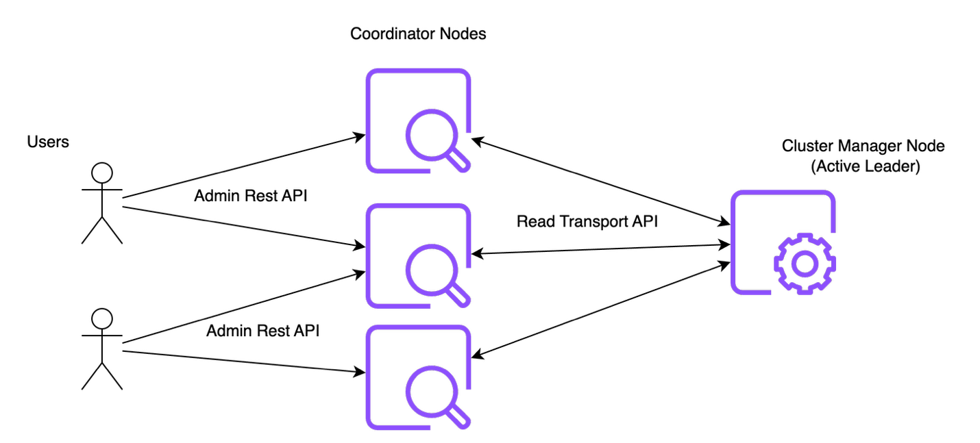
Amazon OpenSearch Service is a managed service that makes it simple to deploy, secure, and operate OpenSearch clusters at scale in the AWS Cloud. A typical OpenSearch cluster is comprised of cluster manager, data, and coordinator nodes. It is recommended to have three cluster manager nodes, and one of them will be elected as a leader node.
Amazon OpenSearch Service introduced support for 1,000-node OpenSearch Service clusters capable of handling 500,000 shards with OpenSearch Service version 2.17. For large clusters, we have identified bottlenecks in admin API interactions (with the leader) and introduced improvements in OpenSearch Service version 2.17. These improvements have helped OpenSearch Service to publish cluster metrics and monitor at same frequency for large clusters while maintaining the optimal resource usage (less than 10% CPU and less than 75% JVM usage) on the leader node (16 core CPU with 64 GB JVM heap). It has also ensured that metadata management can be performed on large clusters with predictable latency without destabilizing the leader node.
General monitoring of an OpenSearch node using health check and statistics API endpoints doesn’t cause visible load to the leader. But as the number of nodes increase in the cluster, the volume of these monitoring calls also increases proportionally. The increase in the call volume coupled with the less optimal implementation of these endpoints overwhelms the leader node, resulting in stability issues. In this post, we demonstrate the different bottlenecks that were identified and the corresponding solutions that were implemented in OpenSearch Service to scale cluster manager for large cluster deployments. These optimizations are available to all new domains or existing domains upgraded to OpenSearch Service versions 2.17 or above.
To understand the various bottlenecks with the cluster manager, let’s examine the cluster state, whose management is the core operation of the leader. The cluster state contains the following key metadata information:
Node, index, and shard are managed as first-class entities by the cluster manager and contain information such as identifier, name, and attributes for each of their instances.
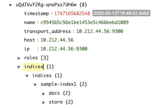
The following screenshots are from a sample cluster state for a cluster with three cluster manager and three data nodes. The cluster has a single index (sample-index1) with one primary and two replicas.
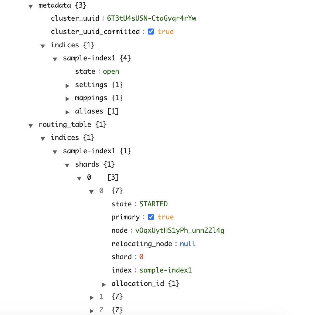
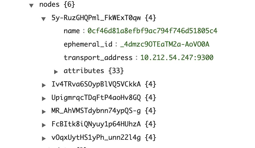
As shown in the screenshots, the number of entries in the cluster state is as follows:
IndexMetadata (metadata#indices) has entries equal to the total number of indexesRoutingTable (routing_table) has entries equal to the number of indexes multiplied by the number of shards per indexNodeInfo (nodes) has entries equal to the number of nodes in the clusterThe size of a sample cluster state with six nodes, one index, and three shards is around 15 KB (size of JSON response from the API). Consider a cluster with 1,000 nodes, which has 10,000 indexes with an average of 50 shards per index. The cluster state would have 10,000 entries for IndexMetadata, 500,000 entries for RoutingTable, and 1,000 entries for NodeInfo.
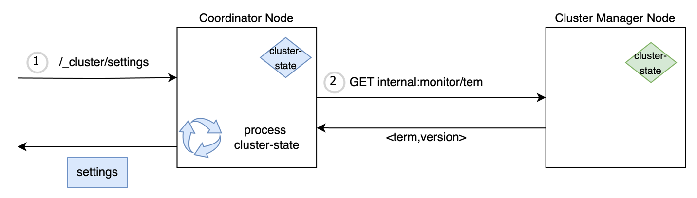
OpenSearch provides admin APIs as a REST endpoint for users to manage and configure the cluster metadata. Admin API requests are handled by either coordinator node (or) by data node if the cluster does not have dedicated coordinator node provisioned. You can use admin APIs to check cluster health, modify settings, retrieve statistics, and more. Some of the examples are the CAT, Cluster Settings, and Node Stats APIs.
The following diagram illustrates the admin API control flow.
Let’s consider a Read API request to fetch information about the cluster settings.
The cluster state processing on the nodes is shown in the following diagram.
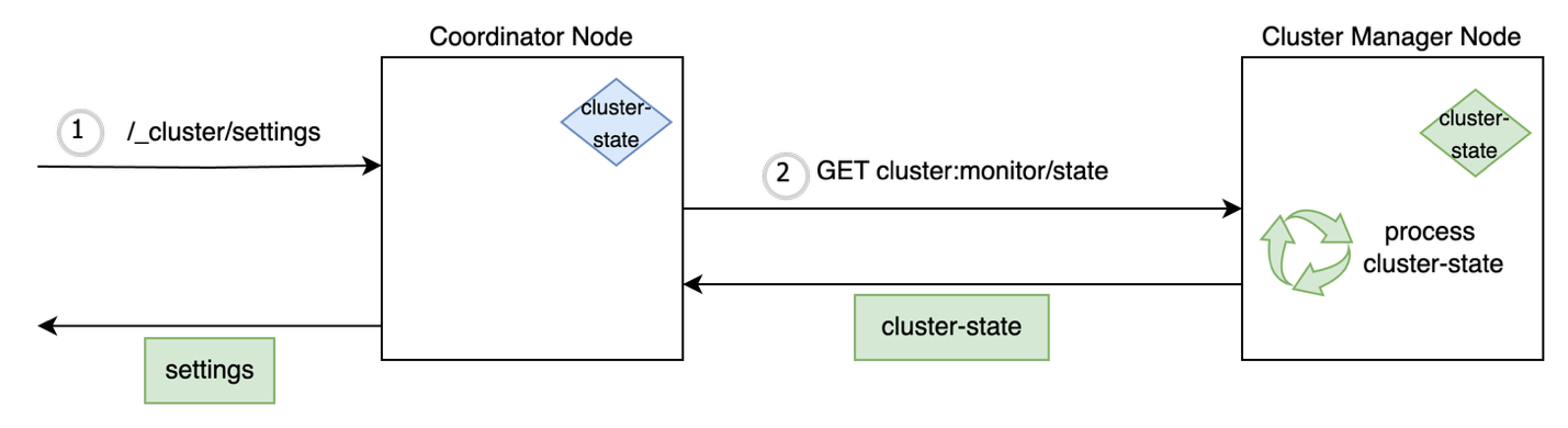
As discussed earlier, most of the admin read requests require the latest cluster state and the node which processes the API request and makes a _cluster/state call to the leader. In a cluster setup of 1,000 nodes and 500,000 shards, the size of the cluster state would be around 250 MB. This can overload leader and cause the following issues:
The leader node sends periodic ping requests to follower nodes and requires transport threads to process the responses. Because the number of threads serving the transport channel is limited (defaults to the number of processor cores), the responses are not processed in a timely fashion. The leader-follower health checks in the cluster get timed out, thereby causing a spiral effect of nodes leaving the cluster and more shard recoveries being initiated by the leader.
Cluster state is versioned using two long fields: term and version. The term number is incremented whenever a new leader is elected, and the version number is incremented with every metadata update. Given that the latest cluster state is cached on all the nodes, it can be used to serve the admin API request if it is up-to-date with the leader. To check the freshness of the cached copy, a light-weight transport API is introduced, which fetches only the term and version corresponding to the latest cluster state from leader. The request-coordinating node matches it with the local term and version, and if they’re the same, it uses the local cluster sate to serve the admin API read request. If the cached cluster state is out of sync, the node makes a subsequent transport call to fetch the latest cluster state and then serves the incoming API request. This offloads the responsibility of serving read requests to the coordinating node, thereby reducing the load on the leader node.
Cluster state processing on the nodes after the optimization is shown in the following diagram.
Term-version checks for cluster state processing are now used by 17 read APIs across the _cat and _cluster APIs in OpenSearch.
From our load tests, we observed at least 50% reduction in CPU usage without a change in the API latency due to the aforementioned improvement. The load test was performed on an OpenSearch cluster consisting of 3 cluster manager nodes (8 cores each), 5 data nodes (64 cores each), and 25,000 shards with a cluster state size of around 50 MB. The workload consists of the following admin APIs invoked, with periodicity mentioned in the following table:
/_cluster/state/_cat/indices/_cat/shards/_cat/allocation| Request Count / 5 minutes | CPU (max) | |
| Existing Setup | With Optimization | |
| 3000 | 14% | 7% |
| 6000 | 20% | 10% |
| 9000 | 28% | 12% |
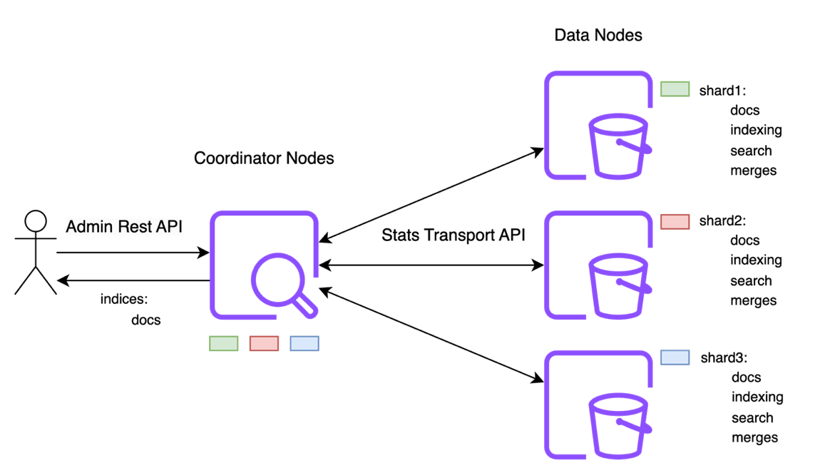
The next group of admin APIs are used to fetch the statistics information of the cluster. These APIs include _cat/indices, _cat/shards, _cat/segments, _cat/nodes, _cluster/stats, and _nodes/stats, to name a few. Unlike metadata, which is managed by the leader, the statistics information is distributed across the data nodes in the cluster.
For example, consider the response to the _cat/indices API for the index sample-index1:
The values for fields docs.count, docs.deleted , store.size, and pri.store.size are fetched from the data nodes, which have the corresponding shards, and are then aggregated by the coordinating node. To compute the preceding response for sample-index1, the coordinator node collects the statistics responses from three data nodes hosting one primary and two replica shards, respectively.
Every data node in the cluster collects statistics related to operations such as indexing, search, merges, and flushes for the shards it manages. Every shard in the cluster has about 150 indices metrics tracked across 20 metric groups.
The response from the data node to coordinator contains all the shard statistics of the index and not just the ones (docs and store stats) requested by the user. The response size of stats returned from data node for a single shard is around 4 KB. The following diagram illustrates the stats data flow among nodes in a cluster.
For a cluster with 500,000 shards, the coordinator node needs to retrieve stats responses from different nodes whose sizes sum to around 2.5 GB. The retrieval of such large response sizes can cause the following issues:
The memory pressure can cause a circuit breaker of the coordinator node to trip, resulting in 429 TOO MANY REQUEST responses. It also results in an increase in CPU utilization on the coordinator node due to garbage collection cycles being triggered to reclaim the heap used for stats requests. The overloading of the coordinator node to fetch statistics information for admin requests can potentially result in rejecting critical API requests such as health check, search, and indexing, resulting in a spiral effect of failures.
Because the admin API returns only the user-requested stats in the response, it is not required by data nodes to send the entire shard-level stats because it’s not requested by the user. We have now introduced stats aggregation at transport action so each data node aggregates the stats locally and then responds back to the coordinator node. Additionally, data nodes support filtering of statistics so only specific shard stats, as requested by the user, can be returned to the coordinator. This results in reduced compute and memory on coordinator nodes because they now work with responses that are far smaller.
The following output is the shard stats returned by a data node to the coordinator node after local aggregation by index. The response is also filtered based on user-requested statistics. The response contains only docs and store metrics aggregated by index for shards present on the node.
The following table shows the latency for health and stats API endpoints in a large cluster. These results are for a cluster size of 3 cluster manager nodes, 1,000 data nodes, and 500,000 shards. As explained in the following pull request, the optimization to pre-compute statistics prior to sending response helps reduce response size and improve latency.
| API | Response Latency | |
| Existing Setup | With Optimization | |
| _cluster/stats | 15s | 0.65s |
| _nodes/stats | 13.74s | 1.69s |
| _cluster/health | 0.56s | 0.15s |
With admin APIs, users can specify the timeout parameter as part of the request. This helps the client fail fast if requests are taking more time to be processed due to an overloaded leader or data node. However, the coordinator node continues to process the request and initiate internal transport requests to data nodes even after the user’s request gets disconnected. This is wasteful work and causes unnecessary load on the cluster because the response from the data node is discarded by the coordinator after the request has timed out. No mechanism exists for the coordinator to track that the request has been cancelled by the user and further downstream transport calls don’t need to be attempted.
To prevent long-running transport requests for admin APIs and reduce the overhead on the already overwhelmed data nodes, cancellation has been implemented at the transport layer. This is now used by the coordinator to cancel the transport requests to data nodes after the user-specified timeout expires.
The _cat/shards API fails gracefully if the leader is overloaded in case of large clusters. The API returns a timeout response to the user without issuing broadcast calls to data nodes.
Let’s now look at challenges with the popular _cat APIs. Historically, CAT APIs didn’t support pagination because the metadata wasn’t expected to grow to tens of thousands in size when it was designed. This assumption no longer holds for large clusters and can cause compute and memory spikes while serving these APIs.
After careful deliberations with the community, we introduced a new set of paginated list APIs for metadata retrieval. The APIs _list/indices and _list/shards are pagination counterparts to _cat/indices and _cat/shards. The _list APIs maintain pagination stability, so that a paginated dataset maintains order and consistency even when a new index is added or an existing index is removed. This is achieved by using a combination of index creation timestamps and index names as page tokens.
_list/shards can now successfully return paginated responses for a cluster with 500,000 shards without getting timed out. Fixed response sizes facilitate faster data retrieval without overwhelming the cluster for large datasets.
Admin API’s are critical for observability and metadata management of OpenSearch domains. Admin APIs, if not designed properly, introduce bottlenecks in the system and impacts the performance of OpenSearch domains. The improvements made for these APIs in version 2.17 have performance gains for all customers of OpenSearch service irrespective of whether it is large-sized (1,000 nodes), mid-sized (200 nodes), or small-sized (20 nodes). It ensures that elected cluster manager node is stable even when the API’s are exercised for domains with large metadata size. OpenSearch is an open source, community-driven software. The foundational pieces of APIs such as pagination, cancellation, and local aggregation are extensible and can be used for other APIs.
If you would like to contribute to OpenSearch, open up a GitHub issue and let us know your thoughts. You could get started with these open PR’s in Github [PR1] [PR2] [PR3] [PR4].
Post Syndicated from Shahna Campbell original https://aws.amazon.com/blogs/security/how-to-develop-an-aws-security-hub-poc/
The enhanced AWS Security Hub (currently in public preview) prioritizes your critical security issues and helps you respond at scale to protect your environment. It detects critical issues by correlating and enriching signals into actionable insights, enabling streamlined response. You can use these capabilities to gain visibility across your cloud environment through centralized management in a unified cloud security solution. During the preview period, these enhanced Security Hub capabilities are available at no additional cost. While the integrated services—Amazon GuardDuty, Amazon Inspector, Amazon Macie, and AWS Security Hub Cloud Security Posture Management (CSPM)—will continue to incur standard charges, new customers can use the trial periods available at no additional cost for each of these underlying security services. By combining these trials with the Security Hub preview, organizations can conduct comprehensive proof of concept (POC) evaluations without significant upfront investment.
In this blog post, we guide you through how to plan and implement a proof of concept (POC) for Security Hub to assess the implementation, functionality, and value of Security Hub in your environment. We walk you through the following steps:
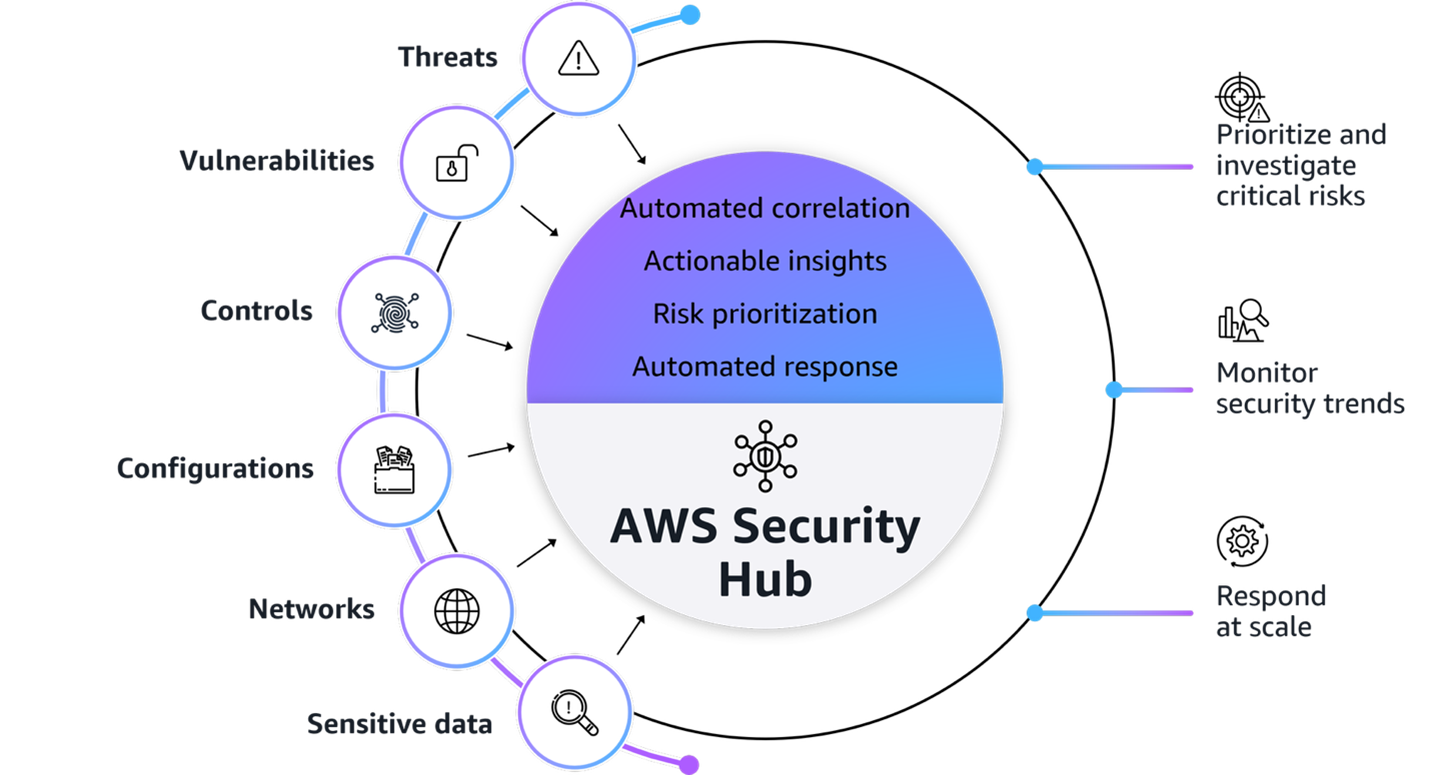
Figure1: AWS Security Hub overview
Figure 1 provides a visualization of how Security Hub unifies signals from multiple AWS security services and capabilities. The signals, which are ingested by Security Hub from multiple AWS security services and capabilities, include:
At its core, Security Hub provides four key capabilities in one unified solution:
With this integrated approach your security team can:
Understand the Open Cybersecurity Schema Framework
Security Hub uses the Open Cybersecurity Schema Framework (OCSF) to help standardize security data and analysis and enable better integration between security tools. This standardization helps simplify how security findings are structured and analyzed across your environment. This standardized data model enables seamless integration and data exchange across your security tooling, providing normalized and consistent data formats. When implementing your Security Hub POC, make sure that you’re familiar with the OCSF specifications. The OCSF schema has eight categories to organize event classes, and each of them are aligned with a specific domain or area of focus. Security Hub uses the Findings category and the classes in the following list.
Additionally, confirm that any analytics or security information and event management (SIEM) tools you plan to integrate with support the OCSF data format to maximize the value of the consolidated security insights provided by Security Hub.
Establishing clear, measurable objectives is fundamental to a successful POC. Begin by defining success metrics that will demonstrate the effectiveness of Security Hub, and whether Security Hub has helped address challenges that you’re facing. Some examples of success criteria include:
After establishing your success criteria, it’s essential to evaluate organizational readiness and potential constraints that might impact your POC implementation. Begin by conducting a comprehensive assessment of your current environment: Are the foundational security services (GuardDuty, Amazon Inspector, Security Hub CSPM, and Macie) enabled across your accounts?
Review your administrative capabilities within AWS Organizations to verify that you have the necessary permissions and control over service deployment. Consider your team’s capacity—do you have dedicated people who can focus on implementation and testing? Additionally, verify that the timing aligns with stakeholder availability for proper evaluation and feedback.
To get the most comprehensive evaluation of the capabilities of Security Hub, carefully plan your service activation timeline to optimize the trial periods available at no additional cost. Here’s how to strategically enable services:
Coordinate the activation of foundational security services to maximize their overlapping trial periods available at no additional cost:
Consider enabling these services simultaneously so that you have at least two weeks of overlapping coverage to evaluate the full correlation and risk prioritization capabilities of Security Hub across each service. Optionally, if you want to conduct a POC with minimal configuration because of limitations, you can enable Security Hub CSPM and Amazon Inspector during the initial POC phase to properly assess the results and data.
Note: Document your activation dates and trial expiration dates carefully. Create calendar reminders for trial end dates and schedule your key POC evaluation milestones to occur while services are active. This will help make sure that you can thoroughly assess the unified security operations capabilities of Security Hub when services are running at full capacity.
If you already have one or more of these underlying services enabled, you can proceed to enable the new Security Hub. To fully use the new Security Hub capabilities, particularly the exposure findings feature, specific service dependencies must be met, both Security Hub CSPM and Amazon Inspector are essential because they provide the foundational data needed for the Security Hub correlation engine and exposure findings features. The combination enables Security Hub to deliver comprehensive risk analysis and prioritization by correlating configuration risks with runtime vulnerabilities. If you have other security services already enabled (such as GuardDuty or Macie), you can maintain these existing services while enabling Security Hub, and it will automatically begin incorporating their findings into its consolidated view, enhancing your overall security posture visualization.
To maximize the value of your Security Hub POC you can use this GuardDuty findings tester repository hosted in the AWS Labs GitHub account and discussed in the Testing and evaluating GuardDuty detections. This repository contains scripts and guidance that you can use as a POC to generate GuardDuty findings related to real AWS resources. There are multiple tests that can be run independently or together depending on the findings you want to generate.
These findings are correlated with Security Hub CSPM control checks to detect misconfigurations and Inspector for vulnerabilities as shown in Figure 2. The example shows the finding page for a Potential Remote Execution finding: Lambda function has network-exploitable software vulnerabilities with a high likelihood of exploitation. The Potential attack path shows that the Lambda function can be exploited remotely over the network with no user interaction or special privileges.
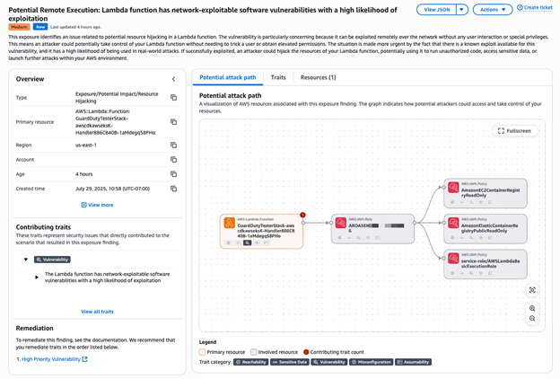
Figure 2: Potential remote execution exposure finding
Note: It’s recommended that you deploy these tests in a non-production account to help make sure that findings generated by these tests can be clearly identified.
After your success criteria have been established, you’re ready to plan your configuration. Some important decisions include:
After you determine your success criteria and your Security Hub configuration, you should have an idea of your stakeholders, desired state, and timeframe. Now, you need to prepare for deployment. In this step, you should complete as much as possible before you deploy Security Hub. The following are some steps to take:
AWS security services integrate with AWS Organizations to help you centrally manage Security Hub.
Note: As a best practice, we recommend using the same delegated administrator across security services for consistent governance.
Note: After you enable Security Hub, exposure findings in your environment are created and analyzed immediately. However, it can take up to 6 hours to receive an exposure finding for a resource.
The final step is to confirm that Security Hub is configured correctly and evaluate the solution against your success criteria.
You might want to remove Security Hub if you do not plan to move forward with deploying into production or need to gain approvals before continuing to use Security Hub. To properly clean up your test environment make sure you address each item below:
In this post, we showed you how to plan and implement a Security Hub POC. You learned how to do so through phases, including defining success criteria, configuring Security Hub, and validating that Security Hub meets your business needs. Remember to use the trial periods to maximize your testing window without incurring significant costs. Throughout the POC, maintain focus on your predefined success criteria while remaining open to unexpected benefits or challenges that may arise. Maintain open communication with your AWS account team to address any questions or concerns to help you get the most out of your Security Hub POC experience.
If you have feedback about this post, submit comments in the Comments section below. If you have questions about this post, contact AWS Support.
Post Syndicated from The Hook Up original https://www.youtube.com/watch?v=F6mFV7XQC3o
Post Syndicated from jzb original https://lwn.net/Articles/1019688/
The openSUSE project is nearing the release of Leap 16, its
first major release since openSUSE Leap 15
in May 2018. This release brings some changes to the
core of the distribution aside from the usual software upgrades; YaST has been retired,
SELinux has replaced AppArmor as the default mandatory access control
(MAC) system, and more. If all goes according to plan, Leap 16
final should be released in early October, with planned support
through 2031.
Post Syndicated from Richard Boulton original https://blog.cloudflare.com/20-percent-internet-upgrade/
Cloudflare is relentless about building and running the world’s fastest network. We have been tracking and reporting on our network performance since 2021: you can see the latest update here.
Building the fastest network requires work in many areas. We invest a lot of time in our hardware, to have efficient and fast machines. We invest in peering arrangements, to make sure we can talk to every part of the Internet with minimal delay. On top of this, we also have to invest in the software we run our network on, especially as each new product can otherwise add more processing delay.
No matter how fast messages arrive, we introduce a bottleneck if that software takes too long to think about how to process and respond to requests. Today we are excited to share a significant upgrade to our software that cuts the median time we take to respond by 10ms and delivers a 25% performance boost, as measured by third-party CDN performance tests.
We’ve spent the last year rebuilding major components of our system, and we’ve just slashed the latency of traffic passing through our network for millions of our customers. At the same time, we’ve made our system more secure, and we’ve reduced the time it takes for us to build and release new products.
Every request that hits Cloudflare starts a journey through our network. It might come from a browser loading a webpage, a mobile app calling an API, or automated traffic from another service. These requests first terminate at our HTTP and TLS layer, then pass into a system we call FL, and finally through Pingora, which performs cache lookups or fetches data from the origin if needed.

FL is the brain of Cloudflare. Once a request reaches FL, we then run the various security and performance features in our network. It applies each customer’s unique configuration and settings, from enforcing WAF rules and DDoS protection to routing traffic to the Developer Platform and R2.
Built more than 15 years ago, FL has been at the core of Cloudflare’s network. It enables us to deliver a broad range of features, but over time that flexibility became a challenge. As we added more products, FL grew harder to maintain, slower to process requests, and more difficult to extend. Each new feature required careful checks across existing logic, and every addition introduced a little more latency, making it increasingly difficult to sustain the performance we wanted.
You can see how FL is key to our system — we’ve often called it the “brain” of Cloudflare. It’s also one of the oldest parts of our system: the first commit to the codebase was made by one of our founders, Lee Holloway, well before our initial launch. We’re celebrating our 15th Birthday this week – this system started 9 months before that!
commit 39c72e5edc1f05ae4c04929eda4e4d125f86c5ce
Author: Lee Holloway <q@t60.(none)>
Date:   Wed Jan 6 09:57:55 2010 -0800

    nginx-fl initial configuration
As the commit implies, the first version of FL was implemented based on the NGINX webserver, with product logic implemented in PHP. After 3 years, the system became too complex to manage effectively, and too slow to respond, and an almost complete rewrite of the running system was performed. This led to another significant commit, this time made by Dane Knecht, who is now our CTO.
commit bedf6e7080391683e46ab698aacdfa9b3126a75f
Author: Dane Knecht
Date:   Thu Sep 19 19:31:15 2013 -0700

    remove PHP.
From this point on, FL was implemented using NGINX, the OpenResty framework, and LuaJIT. While this was great for a long time, over the last few years it started to show its age. We had to spend increasing amounts of time fixing or working around obscure bugs in LuaJIT. The highly dynamic and unstructured nature of our Lua code, which was a blessing when first trying to implement logic quickly, became a source of errors and delay when trying to integrate large amounts of complex product logic. Each time a new product was introduced, we had to go through all the other existing products to check if they might be affected by the new logic.
It was clear that we needed a rethink. So, in July 2024, we cut an initial commit for a brand new, and radically different, implementation. To save time agreeing on a new name for this, we just called it “FL2”, and started, of course, referring to the original FL as “FL1”.
commit a72698fc7404a353a09a3b20ab92797ab4744ea8
Author: Maciej Lechowski
Date:   Wed Jul 10 15:19:28 2024 +0100

Create fl2 projectWe weren’t starting from scratch. We’ve previously blogged about how we replaced another one of our legacy systems with Pingora, which is built in the Rust programming language, using the Tokio runtime. We’ve also blogged about Oxy, our internal framework for building proxies in Rust. We write a lot of Rust, and we’ve gotten pretty good at it.
We built FL2 in Rust, on Oxy, and built a strict module framework to structure all the logic in FL2.
When we set out to build FL2, we knew we weren’t just replacing an old system; we were rebuilding the foundations of Cloudflare. That meant we needed more than just a proxy; we needed a framework that could evolve with us, handle the immense scale of our network, and let teams move quickly without sacrificing safety or performance.
Oxy gives us a powerful combination of performance, safety, and flexibility. Built in Rust, it eliminates entire classes of bugs that plagued our Nginx/LuaJIT-based FL1, like memory safety issues and data races, while delivering C-level performance. At Cloudflare’s scale, those guarantees aren’t nice-to-haves, they’re essential. Every microsecond saved per request translates into tangible improvements in user experience, and every crash or edge case avoided keeps the Internet running smoothly. Rust’s strict compile-time guarantees also pair perfectly with FL2’s modular architecture, where we enforce clear contracts between product modules and their inputs and outputs.
But the choice wasn’t just about language. Oxy is the culmination of years of experience building high-performance proxies. It already powers several major Cloudflare services, from our Zero Trust Gateway to Apple’s iCloud Private Relay, so we knew it could handle the diverse traffic patterns and protocol combinations that FL2 would see. Its extensibility model lets us intercept, analyze, and manipulate traffic from layer 3 up to layer 7, and even decapsulate and reprocess traffic at different layers. That flexibility is key to FL2’s design because it means we can treat everything from HTTP to raw IP traffic consistently and evolve the platform to support new protocols and features without rewriting fundamental pieces.
Oxy also comes with a rich set of built-in capabilities that previously required large amounts of bespoke code. Things like monitoring, soft reloads, dynamic configuration loading and swapping are all part of the framework. That lets product teams focus on the unique business logic of their module rather than reinventing the plumbing every time. This solid foundation means we can make changes with confidence, ship them quickly, and trust they’ll behave as expected once deployed.
One of the most impactful improvements Oxy brings is handling of restarts. Any software under continuous development and improvement will eventually need to be updated. In desktop software, this is easy: you close the program, install the update, and reopen it. On the web, things are much harder. Our software is in constant use and cannot simply stop. A dropped HTTP request can cause a page to fail to load, and a broken connection can kick you out of a video call. Reliability is not optional.
In FL1, upgrades meant restarts of the proxy process. Restarting a proxy meant terminating the process entirely, which immediately broke any active connections. That was particularly painful for long-lived connections such as WebSockets, streaming sessions, and real-time APIs. Even planned upgrades could cause user-visible interruptions, and unplanned restarts during incidents could be even worse.
Oxy changes that. It includes a built-in mechanism for graceful restarts that lets us roll out new versions without dropping connections whenever possible. When a new instance of an Oxy-based service starts up, the old one stops accepting new connections but continues to serve existing ones, allowing those sessions to continue uninterrupted until they end naturally.
This means that if you have an ongoing WebSocket session when we deploy a new version, that session can continue uninterrupted until it ends naturally, rather than being torn down by the restart. Across Cloudflare’s fleet, deployments are orchestrated over several hours, so the aggregate rollout is smooth and nearly invisible to end users.
We take this a step further by using systemd socket activation. Instead of letting each proxy manage its own sockets, we let systemd create and own them. This decouples the lifetime of sockets from the lifetime of the Oxy application itself. If an Oxy process restarts or crashes, the sockets remain open and ready to accept new connections, which will be served as soon as the new process is running. That eliminates the “connection refused” errors that could happen during restarts in FL1 and improves overall availability during upgrades.
We also built our own coordination mechanisms in Rust to replace Go libraries like tableflip with shellflip. This uses a restart coordination socket that validates configuration, spawns new instances, and ensures the new version is healthy before the old one shuts down. This improves feedback loops and lets our automation tools detect and react to failures immediately, rather than relying on blind signal-based restarts.
To avoid the problems we had in FL1, we wanted a design where all interactions between product logic were explicit and easy to understand.
So, on top of the foundations provided by Oxy, we built a platform which separates all the logic built for our products into well-defined modules. After some experimentation and research, we designed a module system which enforces some strict rules:
No IO (input or output) can be performed by the module.
The module provides a list of phases.
Phases are evaluated in a strictly defined order, which is the same for every request.
Each phase defines a set of inputs which the platform provides to it, and a set of outputs which it may emit.
Here’s an example of what a module phase definition looks like:
Phase {
    name: phases::SERVE_ERROR_PAGE,
    request_types_enabled: PHASE_ENABLED_FOR_REQUEST_TYPE,
    inputs: vec![
        InputKind::IPInfo,
        InputKind::ModuleValue(
            MODULE_VALUE_CUSTOM_ERRORS_FETCH_WORKER_RESPONSE.as_str(),
        ),
        InputKind::ModuleValue(MODULE_VALUE_ORIGINAL_SERVE_RESPONSE.as_str()),
        InputKind::ModuleValue(MODULE_VALUE_RULESETS_CUSTOM_ERRORS_OUTPUT.as_str()),
        InputKind::ModuleValue(MODULE_VALUE_RULESETS_UPSTREAM_ERROR_DETAILS.as_str()),
        InputKind::RayId,
        InputKind::StatusCode,
        InputKind::Visitor,
    ],
    outputs: vec![OutputValue::ServeResponse],
    filters: vec![],
    func: phase_serve_error_page::callback,
}
This phase is for our custom error page product. It takes a few things as input — information about the IP of the visitor, some header and other HTTP information, and some “module values.” Module values allow one module to pass information to another, and they’re key to making the strict properties of the module system workable. For example, this module needs some information that is produced by the output of our rulesets-based custom errors product (the “MODULE_VALUE_RULESETS_CUSTOM_ERRORS_OUTPUT” input). These input and output definitions are enforced at compile time.
While these rules are strict, we’ve found that we can implement all our product logic within this framework. The benefit of doing so is that we can immediately tell which other products might affect each other.
Building a framework is one thing. Building all the product logic and getting it right, so that customers don’t notice anything other than a performance improvement, is another.
The FL code base supports 15 years of Cloudflare products, and it’s changing all the time. We couldn’t stop development. So, one of our first tasks was to find ways to make the migration easier and safer.
It’s a big enough distraction from shipping products to customers to rebuild product logic in Rust. Asking all our teams to maintain two versions of their product logic, and reimplement every change a second time until we finished our migration was too much.
So, we implemented a layer in our old NGINX and OpenResty based FL which allowed the new modules to be run. Instead of maintaining a parallel implementation, teams could implement their logic in Rust, and replace their old Lua logic with that, without waiting for the full replacement of the old system.
For example, here’s part of the implementation for the custom error page module phase defined earlier (we’ve cut out some of the more boring details, so this doesn’t quite compile as-written):
pub(crate) fn callback(_services: &mut Services, input: &Input<'_>) -> Output {
    // Rulesets produced a response to serve - this can either come from a special
    // Cloudflare worker for serving custom errors, or be directly embedded in the rule.
    if let Some(rulesets_params) = input
        .get_module_value(MODULE_VALUE_RULESETS_CUSTOM_ERRORS_OUTPUT)
        .cloned()
    {
        // Select either the result from the special worker, or the parameters embedded
        // in the rule.
        let body = input
            .get_module_value(MODULE_VALUE_CUSTOM_ERRORS_FETCH_WORKER_RESPONSE)
            .and_then(|response| {
                handle_custom_errors_fetch_response("rulesets", response.to_owned())
            })
            .or(rulesets_params.body);

        // If we were able to load a body, serve it, otherwise let the next bit of logic
        // handle the response
        if let Some(body) = body {
            let final_body = replace_custom_error_tokens(input, &body);

            // Increment a metric recording number of custom error pages served
            custom_pages::pages_served("rulesets").inc();

            // Return a phase output with one final action, causing an HTTP response to be served.
            return Output::from(TerminalAction::ServeResponse(ResponseAction::OriginError {
                rulesets_params.status,
                source: "rulesets http_custom_errors",
                headers: rulesets_params.headers,
                body: Some(Bytes::from(final_body)),
            }));
        }
    }
}
The internal logic in each module is quite cleanly separated from the handling of data, with very clear and explicit error handling encouraged by the design of the Rust language.
Many of our most actively developed modules were handled this way, allowing the teams to maintain their change velocity during our migration.

It’s essential to have a seriously powerful test framework to cover such a migration. We built a system, internally named Flamingo, which allows us to run thousands of full end-to-end test requests concurrently against our production and pre-production systems. The same tests run against FL1 and FL2, giving us confidence that we’re not changing behaviours.
Whenever we deploy a change, that change is rolled out gradually across many stages, with increasing amounts of traffic. Each stage is automatically evaluated, and only passes when the full set of tests have been successfully run against it – as well as overall performance and resource usage metrics being within acceptable bounds. This system is fully automated, and pauses or rolls back changes if the tests fail.
The benefit is that we’re able to build and ship new product features in FL2 within 48 hours – where it would have taken weeks in FL1. In fact, at least one of the announcements this week involved such a change!
Over 100 engineers have worked on FL2, and we have over 130 modules. And we’re not quite done yet. We’re still putting the final touches on the system, to make sure it replicates all the behaviours of FL1.
So how do we send traffic to FL2 without it being able to handle everything? If FL2 receives a request, or a piece of configuration for a request, that it doesn’t know how to handle, it gives up and does what we’ve called a fallback – it passes the whole thing over to FL1. It does this at the network level – it just passes the bytes on to FL1.
As well as making it possible for us to send traffic to FL2 without it being fully complete, this has another massive benefit. When we have implemented a piece of new functionality in FL2, but want to double check that it is working the same as in FL1, we can evaluate the functionality in FL2, and then trigger a fallback. We are able to compare the behaviour of the two systems, allowing us to get a high confidence that our implementation was correct.
We started running customer traffic through FL2 early in 2025, and have been progressively increasing the amount of traffic served throughout the year. Essentially, we’ve been watching two graphs: one with the proportion of traffic routed to FL2 going up, and another with the proportion of traffic failing to be served by FL2 and falling back to FL1 going down.
We started this process by passing traffic for our free customers through the system. We were able to prove that the system worked correctly, and drive the fallback rates down for our major modules. Our Cloudflare Community MVPs acted as an early warning system, smoke testing and flagging when they suspected the new platform might be the cause of a new reported problem. Crucially their support allowed our team to investigate quickly, apply targeted fixes, or confirm the move to FL2 was not to blame.
We then advanced to our paying customers, gradually increasing the amount of customers using the system. We also worked closely with some of our largest customers, who wanted the performance benefits of FL2, and onboarded them early in exchange for lots of feedback on the system.
Right now, most of our customers are using FL2. We still have a few features to complete, and are not quite ready to onboard everyone, but our target is to turn off FL1 within a few more months.
As we described at the start of this post, FL2 is substantially faster than FL1. The biggest reason for this is simply that FL2 performs less work. You might have noticed in the module definition example a line
filters: vec![],Every module is able to provide a set of filters, which control whether they run or not. This means that we don’t run logic for every product for every request — we can very easily select just the required set of modules. The incremental cost for each new product we develop has gone away.
Another huge reason for better performance is that FL2 is a single codebase, implemented in a performance focussed language. In comparison, FL1 was based on NGINX (which is written in C), combined with LuaJIT (Lua, and C interface layers), and also contained plenty of Rust modules. In FL1, we spent a lot of time and memory converting data from the representation needed by one language, to the representation needed by another.
As a result, our internal measures show that FL2 uses less than half the CPU of FL1, and much less than half the memory. That’s a huge bonus — we can spend the CPU on delivering more and more features for our customers!
Using our own tools and independent benchmarks like CDNPerf, we measured the impact of FL2 as we rolled it out across the network. The results are clear: websites are responding 10 ms faster at the median, a 25% performance boost.

FL2 is also more secure by design than FL1. No software system is perfect, but the Rust language brings us huge benefits over LuaJIT. Rust has strong compile-time memory checks and a type system that avoids large classes of errors. Combine that with our rigid module system, and we can make most changes with high confidence.
Of course, no system is secure if used badly. It’s easy to write code in Rust, which causes memory corruption. To reduce risk, we maintain strong compile time linting and checking, together with strict coding standards, testing and review processes.
We have long followed a policy that any unexplained crash of our systems needs to be investigated as a high priority. We won’t be relaxing that policy, though the main cause of novel crashes in FL2 so far has been due to hardware failure. The massively reduced rates of such crashes will give us time to do a good job of such investigations.
We’re spending the rest of 2025 completing the migration from FL1 to FL2, and will turn off FL1 in early 2026. We’re already seeing the benefits in terms of customer performance and speed of development, and we’re looking forward to giving these to all our customers.
We have one last service to completely migrate. The “HTTP & TLS Termination” box from the diagram way back at the top is also an NGINX service, and we’re midway through a rewrite in Rust. We’re making good progress on this migration, and expect to complete it early next year.
After that, when everything is modular, in Rust and tested and scaled, we can really start to optimize! We’ll reorganize and simplify how the modules connect to each other, expand support for non-HTTP traffic like RPC and streams, and much more.
If you’re interested in being part of this journey, check out our careers page for open roles – we’re always looking for new talent to help us to help build a better Internet.
Post Syndicated from Mingwei Zhang original https://blog.cloudflare.com/monitoring-as-sets-and-why-they-matter/
An AS-SET, not to be confused with the recently deprecated BGP AS_SET, is an Internet Routing Registry (IRR) object that allows network operators to group related networks together. AS-SETs have been used historically for multiple purposes such as grouping together a list of downstream customers of a particular network provider. For example, Cloudflare uses the AS13335:AS-CLOUDFLARE AS-SET to group together our list of our own Autonomous System Numbers (ASNs) and our downstream Bring-Your-Own-IP (BYOIP) customer networks, so we can ultimately communicate to other networks whose prefixes they should accept from us.
In other words, an AS-SET is currently the way on the Internet that allows someone to attest the networks for which they are the provider. This system of provider authorization is completely trust-based, meaning it’s not reliable at all, and is best-effort. The future of an RPKI-based provider authorization system is coming in the form of ASPA (Autonomous System Provider Authorization), but it will take time for standardization and adoption. Until then, we are left with AS-SETs.
Because AS-SETs are so critical for BGP routing on the Internet, network operators need to be able to monitor valid and invalid AS-SET memberships for their networks. Cloudflare Radar now introduces a transparent, public listing to help network operators in our routing page per ASN.
AS-SETs are a critical component of BGP policies, and often paired with the expressive Routing Policy Specification Language (RPSL) that describes how a particular BGP ASN accepts and propagates routes to other networks. Most often, networks use AS-SET to express what other networks should accept from them, in terms of downstream customers.
Back to the AS13335:AS-CLOUDFLARE example AS-SET, this is published clearly on PeeringDB for other peering networks to reference and build filters against.

When turning up a new transit provider service, we also ask the provider networks to build their route filters using the same AS-SET. Because BGP prefixes are also created in IRR registries using the route or route6 objects, peers and providers now know what BGP prefixes they should accept from us and deny the rest. A popular tool for building prefix-lists based on AS-SETs and IRR databases is bgpq4, and it’s one you can easily try out yourself.

For example, to generate a Juniper router’s IPv4 prefix-list containing prefixes that AS13335 could propagate for Cloudflare and its customers, you may use:
% bgpq4 -4Jl CLOUDFLARE-PREFIXES -m24 AS13335:AS-CLOUDFLARE | head -n 10
policy-options {
replace:
 prefix-list CLOUDFLARE-PREFIXES {
    1.0.0.0/24;
    1.0.4.0/22;
    1.1.1.0/24;
    1.1.2.0/24;
    1.178.32.0/19;
    1.178.32.0/20;
    1.178.48.0/20;
Restricted to 10 lines, actual output of prefix-list would be much greater
This prefix list would be applied within an eBGP import policy by our providers and peers to make sure AS13335 is only able to propagate announcements for ourselves and our customers.
Let’s see how accurate AS-SETs can help prevent route leaks with a simple example. In this example, AS64502 has two providers – AS64501 and AS64503. AS64502 has accidentally messed up their BGP export policy configuration toward the AS64503 neighbor, and is exporting all routes, including those it receives from their AS64501 provider. This is a typical Type 1 Hairpin route leak.

Fortunately, AS64503 has implemented an import policy that they generated using IRR data including AS-SETs and route objects. By doing so, they will only accept the prefixes that originate from the AS Cone of AS64502, since they are their customer. Instead of having a major reachability or latency impact for many prefixes on the Internet because of this route leak propagating, it is stopped in its tracks thanks to the responsible filtering by the AS64503 provider network. Again it is worth keeping in mind the success of this strategy is dependent upon data accuracy for the fictional AS64502:AS-CUSTOMERS AS-SET.
Besides using AS-SETs to group together one’s downstream customers, AS-SETs can also represent other types of relationships, such as peers, transits, or IXP participations.
For example, there are 76 AS-SETs that directly include one of the Tier-1 networks, Telecom Italia / Sparkle (AS6762). Judging from the names of the AS-SETs, most of them are representing peers and transits of certain ASNs, which includes AS6762. You can view this output yourself at https://radar.cloudflare.com/routing/as6762#irr-as-sets

There is nothing wrong with defining AS-SETs that contain one’s peers or upstreams as long as those AS-SETs are not submitted upstream for customer->provider BGP session filtering. In fact, an AS-SET for upstreams or peer-to-peer relationships can be useful for defining a network’s policies in RPSL.
However, some AS-SETs in the AS6762 membership list such as AS-10099 look to attest customer relationships.
% whois -h rr.ntt.net AS-10099 | grep "descr"
descr:          CUHK Customer
We know AS6762 is transit free and this customer membership must be invalid, so it is a prime example of AS-SET misuse that would ideally be cleaned up. Many Internet Service Providers and network operators are more than happy to correct an invalid AS-SET entry when asked to. It is reasonable to look at each AS-SET membership like this as a potential risk of having higher route leak propagation to major networks and the Internet when they happen.
Cloudflare Radar is a hub that showcases global Internet traffic, attack, and technology trends and insights. Today, we are adding IRR AS-SET information to Radar’s routing section, freely available to the public via both website and API access. To view all AS-SETs an AS is a member of, directly or indirectly via other AS-SETs, a user can visit the corresponding AS’s routing page. For example, the AS-SETs list for Cloudflare (AS13335) is available at https://radar.cloudflare.com/routing/as13335#irr-as-sets
The AS-SET data on IRR contains only limited information like the AS members and AS-SET members. Here at Radar, we also enhance the AS-SET table with additional useful information as follows.
Inferred ASN shows the AS number that is inferred to be the creator of the AS-SET. We use PeeringDB AS-SET information match if available. Otherwise, we parse the AS-SET name to infer the creator.
IRR Sources shows which IRR databases we see the corresponding AS-SET. We are currently using the following databases: AFRINIC, APNIC, ARIN, LACNIC, RIPE, RADB, ALTDB, NTTCOM, and TC.
AS Members and AS-SET members show the count of the corresponding types of members.
AS Cone is the count of the unique ASNs that are included by the AS-SET directly or indirectly.
Upstreams is the count of unique AS-SETs that includes the corresponding AS-SET.
Users can further filter the table by searching for a specific AS-SET name or ASN. A toggle to show only direct or indirect AS-SETs is also available.

In addition to listing AS-SETs, we also provide a tree-view to display how an AS-SET includes a given ASN. For example, the following screenshot shows how as-delta indirectly includes AS6762 through 7 additional other AS-SETs. Users can copy or download this tree-view content in the text format, making it easy to share with others.

We built this Radar feature using our publicly available API, the same way other Radar websites are built. We have also experimented using this API to build additional features like a full AS-SET tree visualization. We encourage developers to give this API (and other Radar APIs) a try, and tell us what you think!

We know AS-SETs are hard to keep clean of error or misuse, and even though Radar is making them easier to monitor, the mistakes and misuse will continue. Because of this, we as a community need to push forth adoption of RFC9234 and implementations of it from the major vendors. RFC9234 embeds roles and an Only-To-Customer (OTC) attribute directly into the BGP protocol itself, helping to detect and prevent route leaks in-line. In addition to BGP misconfiguration protection with RFC9234, Autonomous System Provider Authorization (ASPA) is still making its way through the IETF and will eventually help offer an authoritative means of attesting who the actual providers are per BGP Autonomous System (AS).
If you are a network operator and manage an AS-SET, you should seriously consider moving to hierarchical AS-SETs if you have not already. A hierarchical AS-SET looks like AS13335:AS-CLOUDFLARE instead of AS-CLOUDFLARE, but the difference is very important. Only a proper maintainer of the AS13335 ASN can create AS13335:AS-CLOUDFLARE, whereas anyone could create AS-CLOUDFLARE in an IRR database if they wanted to. In other words, using hierarchical AS-SETs helps guarantee ownership and prevent the malicious poisoning of routing information.
While keeping track of AS-SET memberships seems like a chore, it can have significant payoffs in preventing BGP-related incidents such as route leaks. We encourage all network operators to do their part in making sure the AS-SETs you submit to your providers and peers to communicate your downstream customer cone are accurate. Every small adjustment or clean-up effort in AS-SETs could help lessen the impact of a BGP incident later.
Visit Cloudflare Radar for additional insights around (Internet disruptions, routing issues, Internet traffic trends, attacks, Internet quality, etc.). Follow us on social media at @CloudflareRadar (X), https://noc.social/@cloudflareradar (Mastodon), and radar.cloudflare.com (Bluesky), or contact us via e-mail.
Post Syndicated from Tim Kadlec original https://blog.cloudflare.com/introducing-observatory-and-smart-shield/
Modern users expect instant, reliable web experiences. When your application is slow, they don’t just complain — they leave. Even delays as small as 100 ms have been shown to have a measurable impact on revenue, conversions, bounce rate, engagement and more.
If you’re responsible for delivering on these expectations to the users of your product, you know there are many monitoring tools that show you how visitors experience your website, and can let you know when things are slow or causing issues. This is essential, but we believe understanding the condition is only half the story. The real value comes from integrating monitoring and remedies in the same view, giving customers the ability to quickly identify and resolve issues.
That’s why today, we’re excited to launch the new and improved Observatory, now in open beta. This monitoring and observability tool goes beyond charts and graphs, by also telling you exactly how to improve your application’s performance and resilience, and immediately showing you the impact of those changes. And we’re releasing it to all subscription tiers (including Free!), available today.

But wait, there’s more! To make your users’ experience in Cloudflare even faster, we’re launching Smart Shield, available today for all subscription tiers. Using Observatory, you can pinpoint performance bottlenecks, and for many of the most common issues, you can now apply the fix in just a few clicks with our Smart Shield product. Double the fun!
Every day, Cloudflare handles traffic for over 20% of the web, giving us a unique vantage point into what makes websites faster and more resilient. We built Observatory to take advantage of this position, uniting data that is normally scattered across different tools — including real-user data, synthetic testing, error rates, and backend telemetry — into a single platform. This gives you a complete, cohesive picture of your application’s health end-to-end, in one spot, and enables you to easily identify and resolve performance issues.
For this launch, we’re bringing together:
Real-user data: See how your application performs for real people, in the real world.
Back-end telemetry: Break down the lifecycle of a request to pinpoint areas for improvement.
Error rates: Understand the stability of your application at both the edge and origin.
Cache hit ratios: Ensure you’re maximizing the performance of your configuration.
Synthetic testing: Proactively test and monitor key endpoints with powerful, accurate simulations.
Let’s take a quick look at each data set to see how we use them in Observatory.
There are two primary forms of data collection: real-user data and synthetic data. Real-user data are performance metrics collected from real traffic, from real visitors, to your application. It’s how users are actually seeing your application perform in the real world. It’s unpredictable, and covers every scenario.
Synthetic data is data collected using some sort of simulated test (loading a site in a headless browser, making network requests from a testing system to an endpoint, etc.). Tests are run under a predefined set of characteristics — location, network speed, etc. — to provide a consistent baseline.
Both forms of data have their uses, and companies with a strongly established culture of operational excellence tend to use both.
The first data you’ll see when you visit Observatory is real-user data collected with Real User Monitoring (RUM), with a particular focus on the Core Web Vital metrics.

This is very intentional.
Real-user data should be the source of truth when it comes to measuring performance and resiliency of your application. Even the best of synthetic data sources are always going to be an approximation. They cannot cover every possible scenario, and because they are being run from a lab environment, they will not always reveal issues that may be more sporadic and unpredictable.
They’re also the best representation of what your users are experiencing when they access your site and, at the end of the day, that’s why we focus on improving performance, resiliency, and security for our users.
We believe so strongly in the importance of every company having access to accurate, detailed RUM data that we are providing it for free, to all accounts. In fact, we’re about to make our privacy-first analytics — which doesn’t track individual users for analytics — available by default for all free zones (excluding data from EU or UK visitors), no setup necessary. We believe the right thing is arming everyone with detailed, actionable, real-user data, and we want to make it easy.
Front-end performance metrics are our best proxy for understanding the actual user experience of an application and as a result, they work great as key performance indicators (KPI’s).
But they’re not enough. Every primary metric should have some level of supporting diagnostic metrics that help us understand why our user metrics are performing like they are — so that we can quickly identify issues, bottlenecks, and areas of improvement.

While the industry has largely, and rightfully, moved on from Time to First Byte (TTFB) as a primary metric of focus, it still has value as a diagnostic metric. In fact, we analyzed our RUM data and found a very strong connection between Time to First Byte and Largest Contentful Paint.
Google’s recommended thresholds for Time to First Byte are:
Good: <= 800ms
Needs Improvement: > 800ms and <= 1800ms
Poor: > 1800ms
Similarly, their official thresholds for Largest Contentful Paint are:
Good: <= 2500ms
Needs Improvement > 2500ms and <= 4000ms
Poor: > 4000ms
Looking across over 9 billion events, we found that when compared to the average site, sites with a “poor” (>1800ms) TTFB are:
70.1 percentage points less likely to have a “good” LCP
21.9 percentage points more likely to have a “needs improvement” LCP
48.2 percentage points more likely to have a “poor” LCP
TTFB is an ill-defined blackbox, so we’re making a point to break that down into its various subparts so you can quickly pinpoint if the issue is with the connection establishment, the server response time, the network itself, and more. We’ll be working to break this down even further in the coming months as we expose the complete lifecycle of a request so you’re able to pinpoint exactly where the bottlenecks lie.
Degradation in stability and performance are frequently directly connected to configuration changes or an increase in errors. Clear visibility into these characteristics can often cut right to the heart of the issue at hand, as well as point to opportunities for improvement of the overall efficiency and effectiveness of your application.

Observatory prominently surfaces cache hit ratio and error rates for both the edge and origin. This compliments the backend telemetry nicely, and helps to further breakdown the backend metrics you are seeing to help pinpoint areas of improvement.
Take cache hit ratio for example. Intuitively, we know that when content is served from cache on an edge server, it should be faster than when the request has to go all the way back to the origin server. Based on our data, again, that’s exactly what we see.
If we consider our Time To First Byte thresholds again (good is <= 800ms; needs improvement is > 800ms and less than 1800ms; poor is anything over 1800ms), when looking across 9 billion data points as collected by our RUM solution, we see that a whopping 91.7% of all pages served from Cloudflare’s cache have a “good” TTFB compared to 79.7% when the request has to be served from the origin server.
In other words, optimizing origin performance (more on that in a bit) and moving more content to the edge are sure-fire ways to give you a much stronger performance baseline.
While real-user data is our source of truth, synthetic testing and monitoring is important as well. Because tests are run in a more controlled environment (test from this location, at this time, with this criteria, etc.), the resulting data is a lot less noisy and variable. In addition, because there is not a user involved and we don’t have to worry about any observer effect, synthetic tests are able to grab a lot more information about the request and page lifecycle.
As a result, synthetic data tends to work very well for arming engineers with debugging information, as well as providing a cleaner set of data for comparing and contrasting results across different platforms, releases, and other situations.
Observatory provides two different types of synthetic tests.
The first synthetic test is a browser test. A browser test will load the requested page in a headless browser, run Google’s Lighthouse on it to report on key performance metrics, and provide some light suggestions for improvement.

The second type of synthetic test Observatory provides is a network test. This is a brand new test type in Cloudflare, and is focused on giving you a better breakdown of the network and back-end performance of an endpoint.
Each network test will hit the provided endpoint for the test and record the wait time, server response time, connect time, SSL negotiation time, and total load time for the endpoint response. Because these tests are much more targeted, a single test in itself is not as valuable and can be prone to variation. That variation isn’t necessarily a bad thing—in fact, variability in these results can actually give you a better understanding of the breadth of results when real users hit that same endpoint.
For that reason, network tests trigger a series of individual runs against the provided endpoint spread out over a short period of time. The data for each response is recorded, and then presented as a histogram on the test results page, letting you see not just a single datapoint, but the long and short-tail of each metric. This gives you a much more accurate representation of reality than what a single test run can provide.

You are also able to compare network tests in Observatory, by selecting two network tests that have been completed. Again, all the data points for each test will be provided in a histogram, where you can easily compare the results of the two.

We are working on improving both synthetic test types in Q4 2025, focusing on making them more powerful and diagnostic.
As we mentioned before, even at its best, synthetic data is an approximation of what is actually happening. Accuracy is critical. Inaccurate data can distract teams with variability and faulty measurements.
It’s important that these tools are as accurate and true to the real world as possible. It’s also important to us that we give back to the community, both because it’s the right thing to do, and because we believe the best way to have the highest level of confidence in the measurement tools and frameworks we’re using is the rigor and scrutiny that open-source provides.
For those reasons, we’ll be working on open-sourcing many of the testing agents we’re using to power Observatory. We’ll share more on that soon, as well as more details about how we’ve built each different testing tool, and why.
People don’t measure for the sake of having data and pretty charts. They measure because they want to be able to stay on top of the health of their application and find ways to improve it. Data is easy. Understanding what to do about the data you’re presented is both the hardest, and most important, part.
Monitoring without action is useless.
We’re building Observatory to have a relentless focus on actionability. Before any new metric is presented, we take some time to explore why that metric matters, when it’s something worth addressing, and what actions you should take if those metrics need improvement.
All of that leads us to our new Smart Suggestions. Wherever possible, we want to pair each metric with a set of opinionated, data-driven suggestions for how to make things better. We want to avoid vague hand-wavy advice and instead be prescriptive and specific and precise.
For example, let’s look at one particular recommendation we provide around improving Largest Contentful Paint.
Largest Contentful Paint is a core web vital metric that measures when the largest piece of content is displayed on the screen. That piece of content could be an image, video or text.
Much like TTFB, Largest Contentful Paint is a bit of a black box by itself. While it tells us how long it takes for that content to get on screen, there are a large number of potential bottlenecks that could be causing the delay. Perhaps the server response time was very slow. Or maybe there was something blocking the content from being displayed on the page. If the object was an image or video, perhaps the filesize was large and the resulting download was slow. LCP by itself doesn’t give us that level of granularity, so it’s hard to give more than hand wavy guidance on how to address it.
Thankfully, just like we can break TTFB into subparts, we can break LCP into its subparts as well. Specifically we can look at:
Time to First Byte: how quickly the server responds to the request for HTML
Resource Load Delay: How long it takes after TTFB for the browser to discover the LCP resource
Resource Load Duration: How long it takes for the browser to download the LCP resource
Render Delay: How long it takes the browser to render the content, after it has the resource in hand.
Breaking it down into these subparts, we can be much more diagnostic about what to do.

In the example above, our recommendation engine analyzes the site’s real-user data and notices that Resource Load Delay accounts for over 10% of total LCP time. As a result, there’s a high likelihood that the resource triggering LCP is large and could potentially be compressed to reduce file size. So we make a recommendation to enable compression using Polish.
We’re very excited about the impact these suggestions will have on helping everyone quickly zero in on meaningful solutions for improving performance and resiliency, without having to wade through mountains of data to get there. As we analyze data, we’ll find more and more patterns of problems and the solutions they can map to. Expanding on our Smart Suggestions will be a constant and ongoing focus as we move forward, and we are working on adding much more content about those patterns and what we find in Q4.
Observatory gives you unprecedented insight into your application’s health, but insights are only half the battle. The next challenge is acting on them, which brings us to another layer of complexity: protecting your origin. For many of our customers, proper management of origin routes and connections is one of the largest drivers of aggregate overall performance. As we mentioned before, we see a clear negative impact on user-facing performance metrics when we have to go back to the origin, and we want to make it as easy as possible for our customers to improve those experiences. Achieving this requires protecting against unnecessary load while ensuring only trusted traffic reaches your servers.
Today’s customers have powerful tools to protect their origins, but achieving basic use cases remains frustratingly complex:
Making applications faster
Reducing origin load
Understanding origin health issues
Restricting IP address access to origin servers
These fundamental needs currently require navigating multiple APIs and dashboard settings. You shouldn’t need to become an expert in each feature — we should analyze your traffic patterns and provide clear, actionable solutions.
Smart Shield transforms origin protection from a complex, multi-tool challenge into a streamlined, intelligent solution that works on your behalf. Our unified API and UI combines all origin protection essentials — dynamic traffic acceleration, intelligent caching, health monitoring, and dedicated egress IPs — into one place that enables single-click configuration.
But we didn’t stop at simplification. Smart Shield integrates with Observatory to provide both the “what” — identifying performance bottlenecks and health issues — and the “how” — delivering capabilities that increase performance, availability, and security.
This creates a continuous feedback loop: Observatory identifies problems, Smart Shield provides solutions, and real-time analytics verify the impact.


But what does this mean for you?
Reduce total cost of ownership (TCO)
Reduce the time-to-value (TTV) for performance, availability, and security issues pertaining to customer origins
Enable new features without guesswork and validate effectiveness in the data
Your time stays focused on building incredible user experiences, not becoming a configuration expert. We are excited to give you back time for your customers and your engineers, while paving the way for how you make sure your origin infrastructure is easily optimized to delight your customers.
Keeping your origins fast and stable is a big part of what we do at Cloudflare. When you experience a traffic surge, the last thing you want is for a flood of TLS handshakes to knock your origin down, or for those new connections to stall your requests, leaving your users to wait for slow pages to load.
This is why we’ve made significant changes to how Cloudflare’s network talks to your origins to dramatically improve the performance of our origin connections.
When Cloudflare makes a request to your origins, we make them from a subset of the available machines in every Cloudflare data center so that we can improve your connection reuse. Until now, this pool would be sized the same by default for every application within a data center, and changes to the sizing of the pool for a particular customer would need to be made manually. This often led to suboptimal connection reuse for our customers, as we might be making requests from way more machines than were actually needed, resulting in fewer warm connection pools than we otherwise could have had. This also caused issues at our data centers from time to time, as larger applications might have more traffic than the default pool size was capable of serving, resulting in production incidents where engineers are paged and had to manually increase the fanout factor for specific customers.
Now, these pool sizes are determined automatically and dynamically. By tracking domain-level traffic volume within a datacenter, we can automatically scale up and scale down the number of machines that serve traffic destined for customer origin servers for any particular customer, improving both the performance of customer websites and the reliability of our network. A massive, high-volume website with a considerable amount of API traffic will no longer be processed by the same number of machines as a smaller and more typical website. Our systems can respond to changes in customer traffic patterns within seconds, allowing us to quickly ramp up and respond to surges in origin traffic.
Thanks to these improvements, Cloudflare now uses over 30% fewer connections across the board to talk to origins. To put this into a more understandable perspective, this translates to saving approximately 402 years of handshake time every day across our global traffic, or 12,060 years of handshake time saved per month! This means just by proxying your traffic through Cloudflare, you’ll see a 30% on average reduction in the amount of connections to your origin, keeping it more available while serving the same traffic volume and in turn lowering your egress fees. But, in many cases, the results observed can be far greater than 30%. For example, in one data center which is particularly heavy in API traffic, we saw a reduction in origin connections of ~60%!
Many don’t realize that making more connections to an origin requires more compute and time for systems to create TCP and SSL handshakes. This takes time away from serving content requested by your end-users and can act as a hidden tax on your performance and overall to your application. We are proud to reduce the Internet’s hidden tax by finding intelligent, innovative ways to reduce the amount of connections needed while supporting the same traffic volume.
Watch out for more updates to Smart Shield at the start of 2026 — we’re working on adding self-serve support for dedicated CDN egress IP addresses, along with significant performance, reliability, and resilience improvements!
We’re really excited to share these two products with everyone today. Smart Shield and Observatory combine to provide a powerful one-two punch of insight and easy remediation.
As we navigate the beta launch of Observatory, we know this is just the start.
Our vision for Observatory is to be the single source of truth for your application’s health. We know that making the right decisions requires robust, accurate data, and we want to arm our customers with the most comprehensive picture available.
In the coming months, we plan to continue driving forward with our goal of providing comprehensive data, backed by a clear path to action.
Deeper, more diagnostic data. We’ll continue to break down data silos, bringing in more metrics to make sure you have a truly comprehensive view of your application’s health. We’ll be focused on going deeper and being more diagnostic, breaking down every aspect of both the request and page lifecycle to give you more granular data.
More paths to solutions. People don’t measure for the sake of looking at data, they measure to solve problems. We’re going to continue to expand our suggestions, arming you with more precise, data-driven solutions to a wider range of issues, letting you fix problems with a single click through Smart Shield and bringing a tighter feedback loop to validate the impact of your configuration updates.
Benchmarking against other products. Some of our customers split traffic between different CDNs due to regulatory or compliance requirements. Naturally, this brings up a whole series of questions about comparing the performance of the split traffic. In Observatory, you can compare these today, but we have a lot of things planned to make this even easier.
Try out Observatory and Smart Shield yourself today. And if you have ideas or suggestions for making Observatory and Smart Shield better, we’re all ears and would love to talk!
Post Syndicated from Celso Martinho original https://blog.cloudflare.com/an-ai-index-for-all-our-customers/
Today, we’re announcing the private beta of AI Index for domains on Cloudflare, a new type of web index that gives content creators the tools to make their data discoverable by AI, and gives AI builders access to better data for fair compensation.
With AI Index enabled on your domain, we will automatically create an AI-optimized search index for your website, and expose a set of ready-to-use standard APIs and tools including an MCP server, LLMs.txt, and a search API. Our customers will own and control that index and how it’s used, and you will have the ability to monetize access through Pay per crawl and the new x402 integrations. You will be able to use it to build modern search experiences on your own site, and more importantly, interact with external AI and Agentic providers to make your content more discoverable while being fairly compensated.
For AI builders—whether developers creating agentic applications, or AI platform companies providing foundational LLM models—Cloudflare will offer a new way to discover and retrieve web content: direct pub/sub connections to individual websites with AI Index. Instead of indiscriminate crawling, builders will be able to subscribe to specific sites that have opted in for discovery, receive structured updates as soon as content changes, and pay fairly for each access. Access is always at the discretion of the site owner.
From the individual indexes, Cloudflare will also build an aggregated layer, the Open Index, that bundles together participating sites. Builders get a single place to search across collections or the broader web, while every site still retains control and can earn from participation.
AI platforms are quickly becoming one of the main ways people discover information online. Whether asking a chatbot to summarize a news article or find a product recommendation, the path to that answer almost always starts with crawling original content and indexing or using that data for training. However, today, that process is largely controlled by platforms: what gets crawled, how often, and whether the site owner has any input in the matter.
Although Cloudflare now offers to monitor and control how AI services respect your access policies and how they access your content, it’s still challenging to make new content visible. Content creators have no efficient way to signal to AI builders when a page is published or updated. On the other hand, for AI builders, crawling and recrawling unstructured content is costly, wastes resources, especially when you don’t know the quality and cost in advance.
We need a fairer and healthier ecosystem for content discovery and usage that bridges the gap between content creators and AI builders.
When you onboard a domain to Cloudflare, or if you have an existing domain on Cloudflare, you will have the choice to enable an AI Index. If enabled, we will automatically create an AI-optimized search index for your domain that you own and control.

As your site updates and grows, the index will evolve with it. New or updated pages will be processed in real-time using the same technology that powers Cloudflare AI Search (formerly AutoRAG) and its Website as a data source. Best of all, we will manage everything; you won’t have to worry about each individual component of compute, storage resources, databases, embeddings, chunking, or AI models. Everything will happen behind the scenes, automatically.
Importantly, you will have control over what content to include or exclude from your website’s index, and who can get access to your content via AI Crawl Control, ensuring that only the data you want to expose is made searchable and accessible. You also will be able to opt out of the AI Index completely; it will all be up to you.
When your AI Index is set up, you will get a set of ready-to-use APIs:
An MCP Server: Agentic applications will be able to connect directly to your site using the Model Context Protocol (MCP), making your content discoverable to agents in a standardized way. This includes support for NLWeb tools, an open project developed by Microsoft that defines a standard protocol for natural language queries on websites.
A flexible search API: This endpoint will return relevant results in structured JSON.
LLMs.txt and LLMs-full.txt: Standard files that provide LLMs with a machine-readable map of your site, following emerging open standards. These will help models understand how to use your site’s content at inference time. An example of llms.txt exists in the Cloudflare Developer Documentation.
A bulk data API: An endpoint for transferring large amounts of content efficiently, available under the rules you set. Instead of querying for every document, AI providers will be able to ingest in one shot.
Pub-sub subscriptions: AI platforms will be able to subscribe to your site’s index and receive events and content updates directly from Cloudflare in a structured format in real-time, making it easy for them to stay current without re-crawling.
Discoverability directives: In robots.txt and well-known URIs to allow AI agents and crawlers visiting your site to discover and use the available API automatically.

The index will integrate directly with AI Crawl Control, so you will be able to see who’s accessing your content, set rules, and manage permissions. And with Pay per crawl and x402 integrations, you can choose to directly monetize access to your content.
As an AI builder, you will be able to discover and subscribe to high-quality, permissioned web data through individual site’s AI indexes. Instead of sending crawlers blindly across the open Internet, you will connect via a pub/sub model: participating websites will expose structured updates whenever their content changes, and you will be able to subscribe to receive those updates in real-time. With this model, your new workflow may look something like this:
Discover websites that have opted in: Browse and filter through a directory of websites that make their indexes available through Cloudflare.
Evaluate content with metadata and metrics: Get content metadata information on various metrics (e.g., uniqueness, depth, contextual relevance, popularity) before accessing it.
Pay fairly for access: When content is valuable, platforms can compensate creators directly through Pay per crawl. These payments not only enable access but also support the continued creation of original content, helping to sustain a healthier ecosystem for discovery.
Subscribe to updates: Use pub-sub subscriptions to receive events about changes made by the website, so you know when to retrieve or crawl for new content without wasting resources on constant re-crawling.
By shifting from blind crawling to a permissioned pub/sub system for the web, AI builders save time, cut costs, and gain access to cleaner, high-quality data while content creators remain in control and are fairly compensated.
Individual indexes provide AI platforms with the ability to access data directly from specific sites, allowing them to subscribe for updates, evaluate value, and pay for full content access on a per-site basis. But when builders need to work at a larger scale, managing dozens or hundreds of separate subscriptions can become complex. The Open Index will provide an additional option: a bundled, opt-in collection of those indexes, featuring sophisticated features such as quality, uniqueness, originality, and depth of content filters, all accessible in one place.

The Open Index is designed to make content discovery at scale easier:
Get unified access: Query and retrieve data across many participating sites simultaneously. This reduces integration overhead and enables builders to plug into a curated collection of data, or use it as a ready-made web search layer that can be accessed at query time.
Discover broader scopes: Work with topic-specific bundles (e.g., news, documentation, scientific research) or a general discovery index covering the broader web. This makes it simple to explore new content sources you may not have identified individually.
Bottom-up monetization: Results still originate from an individual site’s AI index, with monetization flowing back to that site through Pay per crawl, helping preserve fairness and sustainability at scale.
Together, per-site AI indexes and the Open Index will provide flexibility and precise control when you want full content from individual sites (i.e., for training, AI agents, or search experiences), and broad search coverage when you need a unified search across the web.
With AI Index and the Cloudflare Open Index, we’re creating a model where websites decide how their content is accessed, and AI builders receive structured, reliable data at scale to build a fairer and healthier ecosystem for content discovery and usage on the Internet.
We’re starting with a private beta. If you want to enroll your website into the AI Index or access the pub/sub web feed as an AI builder, you can sign up today.
Post Syndicated from daroc original https://lwn.net/Articles/1039749/
Security updates have been issued by AlmaLinux (firefox, kernel, and thunderbird), Debian (ceph and thunderbird), Fedora (chromium, mingw-expat, python-deepdiff, python-orderly-set, python-pip, rust-az-cvm-vtpm, rust-az-snp-vtpm, rust-az-tdx-vtpm, and trustee-guest-components), Oracle (aide, kernel, and thunderbird), Red Hat (firefox, kernel, openssh, perl-YAML-LibYAML, and thunderbird), Slackware (expat), SUSE (jasper, libssh, openjpeg2, and python-pycares), and Ubuntu (linux-aws-6.14, linux-hwe-6.14, linux-azure, linux-hwe-6.8, linux-realtime-6.8, node-sha.js, and pcre2).
Post Syndicated from David Belson original https://blog.cloudflare.com/new-regional-internet-traffic-and-certificate-transparency-insights-on-radar/
Since launching during Birthday Week in 2020, Radar has announced significant new capabilities and data sets during subsequent Birthday Weeks. We continue that tradition this year with a two-part launch, adding more dimensions to Radar’s ability to slice and dice the Internet.
First, we’re adding regional traffic insights. Regional traffic insights bring a more localized perspective to the traffic trends shown on Radar.
Second, we’re adding detailed Certificate Transparency (CT) data, too. The new CT data builds on the work that Cloudflare has been doing around CT since 2018, including Merkle Town, our initial CT dashboard.
Both features extend Radar’s mission of providing deeper, more granular visibility into the health and security of the Internet. Below, we dig into these new capabilities and data sets.
Cloudflare Radar initially launched with visibility into Internet traffic trends at a national level: want to see how that Internet shutdown impacted traffic in Iraq, or what IPv6 adoption looks like in India? It’s visible on Radar. Just a year and a half later, in March 2022, we launched Autonomous System (ASN) pages on Radar. This has enabled us to bring more granular visibility to many of our metrics: What’s network performance like on AS701 (Verizon Fios)? How thoroughly has AS812 (Rogers Communications) implemented routing security? Did AS58322 (Halasat) just go offline? It’s all visible on Radar.
However, sometimes Internet usage shifts on a more local level — maybe a sporting event in a particular region drives people online to find out more information. Or maybe a storm or other natural disaster causes infrastructure damage and power outages in a given state, impacting Internet traffic.
For the last few years, the Radar team relied on internal data sets and Jupyter notebooks to visualize these “sub-national” traffic shifts. But today, we are bringing that insight to Cloudflare Radar, and to you, with the launch of regional traffic insights. With this new capability, you’ll be able to see traffic trends at a more local level, including bytes and requests, as well as breakouts of desktop/mobile device and bot/human traffic shares. And for even more granular visibility, within the Data Explorer, you’ll also be able to select an autonomous system to join with the regional selection — for example, looking at AS7922 (Comcast) in Massachusetts (United States).
In line with common industry practice, the region names displayed on Radar are sourced in data from GeoNames (geonames.org), a crowdsourced geographical database. Specifically, we are using the “first-order administrative divisions” listed for each country — for example, the states of America, the departments of Honduras, or the provinces of Canada. Those geographical names reflect data provided by GeoNames; for more information, please refer to their About page.
Requests logged by Cloudflare’s services include the IP address of the device making the request. The address range (“prefix”) that includes this address is associated with a GeoNames ID within our IP address geolocation data, and we then match that GeoNames ID with the associated country and “first order administrative division” found in the GeoNames dataset. (For example: 155.246.1.142 → 155.246.0.0/16 → GeoNames ID 5101760 → United States > New Jersey)

Within Cloudflare Radar, there are several ways to get to this regional data. If you know the name of the region of interest, you can type it into the search bar at the top of the page, and select it from the results. For example, beginning to type Massachusetts returns the U.S. state, linked to its regional traffic page. Typing the region name into the Traffic in dropdown at the top of a Traffic page will also return the same set of results.

Radar’s country-level pages now have a new Traffic characteristics by region card that includes both summary and time series views of regional traffic. The summary view is presented as a map and table, similar to the Traffic characteristics card in the Worldwide traffic view. After selecting a metric from the dropdown at the top right of the card, the table and map are updated to reflect the relevant summary values for the chosen time period. Within the paginated table, the region names are linked, and clicking one will take you to the relevant page. Within the map, the summary values are represented by circles placed in the centroid of each region, sized in relation to their value. Clicking a circle will take you to the relevant page.

Below the summary map and table, the card also includes a time series graph of traffic at a regional level for the top five highest traffic regions within the country. These graphs can reveal interesting regional differences in traffic patterns. For example, the Traffic volume by region in Iraq graph for HTTP request traffic shown below highlights the differing Internet shutdown schedules (Kurdistan Region, central and southern Iraq) across the different governorates. On days when the schedules do not overlap, such as September 2 and 7, traffic from the Erbil and Sulaymaniyah governorates, which are located in the Kurdistan Region, does not drop concurrent with the loss in traffic observed in Baghdad and Basra.

Over the past several years, a number of Radar blog posts have explored how human activity impacts Internet traffic, including holiday celebrations, elections, and the Paris 2024 Summer Olympics. With the new regional views, this impact now becomes even clearer at a more local level. For instance, mobile devices account for, on average, just over half of the request traffic seen from Nairobi Country in Kenya. A clear diurnal pattern is seen on weekdays, where mobile device usage drops during workday hours, and then rises again in the evening. However, during the weekends, mobile traffic remains elevated, presumably due to fewer people using desktop computers in office environments, as well as fewer desktop computers in use at home, in line with Kenya’s mobile-first culture.

Similar to how the mobile vs. desktop view exposes shifts in human activity, bot vs. human traffic insights do as well. One interpretation of the graph below is that overnight bot activity from Lisbon increased significantly during the first few days of September. However, since the graph shows traffic shares, and given the timing of the apparent increases, the more likely cause is increasingly larger drops in human-driven traffic – users in Lisbon appear to begin logging off around 23:00 UTC (midnight local time), and start getting back online around 05:00 UTC (06:00 local time). The shares and shifts will obviously vary by country and region, but they can provide a perspective on the nocturnal habits of users in a region.

Within the Data Explorer, you can use the breakdown options and filters to customize your analysis of regional traffic data.
At a country level, choosing to breakdown by regions generates a stacked area graph that shows the relative traffic shares of the top 20 regions in the selected country, along with a bar graph showing summary share values. For example, the graph below shows that in aggregate, Virginia and California are responsible for just over a quarter of the HTTP request volume in the United States.


You can also use Data Explorer to drill down on traffic at a network (ASN) level in a given region, in both summary and timeseries views. For example, looking at HTTP request traffic for Massachusetts by ASN, we can see that AS7922 (Comcast), accounts for a third, followed by AS701 (Verizon Fios, 15%), AS21928 (T-Mobile, 8.8%), AS6167 (Verizon Wireless, 5.1%), AS7018 (AT&T, 4.7%), and AS20115 (Charter/Spectrum, 4.5%). Over 70% of the request traffic is concentrated in these six providers, with nearly half of that from one provider.


Going a level deeper, you can also look at traffic trends over time for an ASN within a given region, and even compare it with another time period. The graph below shows traffic for AS7922 (Comcast) in Massachusetts over a seven-day period, compared with the prior week. While the traffic volumes on most days were largely in line with the previous week, Saturday and Sunday were noticeably higher. These differences may reflect a shift in human activity, as September 6 & 7 were quite rainy in Massachusetts, so people may have spent more time indoors and online. (The prior weekend was Labor Day weekend, but those Saturday and Sunday traffic levels were in line with the preceding weekend.) You can also add another ASN to the traffic trends comparison. Selecting Massachusetts (Location) and AS701 (ASN) (Verizon Fios) in the Compare section finds that traffic on that network was higher on Saturday and Sunday as well, lending credence to the rainy weekend theory.


Regional comparisons, whether within the same country or across different countries, are also possible in Data Explorer. For instance, if the Kansas City Chiefs and Philadelphia Eagles were to meet yet again in the Super Bowl, the configuration below could be used to compare traffic patterns in the teams’ respective home states, as well as comparing the trends with the previous week, showing how human activity impacted it over the course of the game.

As always, the data powering the visualizations described above are also available through the Radar API. The timeseries_groups and summary methods for the NetFlows and HTTP endpoints now have an ADM1 dimension, allowing traffic to be broken down by first-order administrative divisions. In addition, the new geoId filter for the NetFlows and HTTP endpoints allows you to filter the results by a specific geolocation, using its GeoNames ID. And finally, there are new get and list endpoints for fetching geolocation details.
As you’d expect, the more traffic we see from a given geography, the better the “signal”, and the clearer the associated graph is — this is generally the case when traffic is aggregated at a country level. However, for some smaller or less populous regions, especially in developing countries or countries with poor Internet connectivity, lower traffic will likely cause the signal to be weaker, resulting in graphs that appear spiky or incomplete. (Note that this will also be true for region+ASN views.) An illustrative example is shown below, for Northern Darfur State in Sudan. Traffic is observed somewhat inconsistently, resulting in the spikes seen in the graph. Similarly, the “Previous 7 days” line is largely incomplete, indicating a lack of traffic data for that period. In these cases, it will be hard to draw definitive conclusions from such graphs.

Although the Internet arguably transcends geographical boundaries, the reality is that usage patterns can vary by location, with traffic trends that reflect more localized human activity. The new regional insights on Cloudflare Radar traffic pages, and in the Data Explorer, provide a perspective at a sub-national level. We are exploring the potential to go a level deeper in the future, providing traffic data for “second-order administrative divisions” (such as counties, cities, etc.).
If you share our regional traffic graphs on social media, be sure to tag us: @CloudflareRadar (X), noc.social/@cloudflareradar (Mastodon), and radar.cloudflare.com (Bluesky). If you have questions or comments, you can reach out to us on social media, or contact us via email.
Just as we’re bringing more granular detail to traffic patterns, we’re also shedding more light on the very foundation of trust on the Internet: TLS certificates. Certificate Authorities (CAs) serve as trusted gatekeepers for the Internet: any website that wants to prove its identity to clients must present a certificate issued by a CA that the client trusts. But how do we know that CAs themselves are trustworthy and only issue certificates they are authorized to issue?
That’s where Certificate Transparency (CT) comes in. Clients that enforce CT (most major browsers) will only trust a website certificate if it is both signed by a trusted CA and has proof that the certificate has been added to a public, append-only CT log, so that it can be publicly audited. Only recently, CT played a key role in detecting the unauthorized issuance of certificates for 1.1.1.1, a public DNS resolver service that Cloudflare operates.
In addition to its role as a vital safety mechanism for the Internet, CT has proven to be invaluable in other ways, as it provides publicly-accessible lists of all website certificates used on the Internet. This dataset is a treasure trove of intelligence for researchers measuring the Internet, security teams detecting malicious activity like phishing campaigns, or penetration testers mapping a target’s external attack surface.
The sheer amount of data (multiple terabytes) available in CT makes it difficult for regular Internet users to download and explore themselves. Instead, services like crt.sh, Censys, and Merklemap provide easy search interfaces to allow discoverability for specific domain names and certificates. We launched Merkle Town in 2018 to share broad insights into the CT ecosystem using data from our own CT monitoring service.
Certificate Transparency on Cloudflare Radar is the next evolution of Merkle Town, providing integration with security and domain information already on Radar and more interactive ways to explore and analyze CT data. (For long-time Merkle Town users, we’re keeping it around until we’ve reached full feature parity.)
In the sections below, we’ll walk you through the features available in the new dashboard.
The CT page leads with a view of how many certificates are being issued and logged over time. Because the same certificate can appear multiple times within a single log or be submitted to several logs, the total count can be inflated. To address this, two distinct lines are shown: one for total entries and another for unique entries. Uniqueness, however, is calculated only within the selected time range — for example, if certificate C is added to log A in one period and to log B in another, it will appear in the unique count for both periods. It is also important to note that the CT charts and date filters use the log timestamp, which is the time a certificate was added to a CT log. Additionally, the data displayed on the page was collected from the logs monitored by Cloudflare — delays, backlogs, or other inconsistencies may exist, so please report any issues or discrepancies.
Alongside this chart is a comparison between certificates and pre-certificates. A pre-certificate is a special type of certificate used in CT that allows a CA to publicly log a certificate before it is officially issued. CAs are not required to log full certificates if corresponding pre-certificates have already been logged (although many CAs do anyway), so typically there are more pre-certificates logged than full certificates, as seen in the chart.

While certificate issuance trends are interesting on their own, analyzing the characteristics of issued certificates provides deeper insight into the state of the web’s trust infrastructure. Starting with the public key algorithm, which defines how secure connections are established between clients and servers, we found that more than 65% of certificates still use RSA, while the remainder use ECDSA. RSA remains dominant due to its long-standing compatibility with a wide range of clients, while ECDSA is increasingly adopted for its efficiency and smaller key sizes, which can improve performance and reduce computational overhead. In the coming years, we expect post-quantum signature algorithms like ML-DSA to appear when public CAs begin to offer support.
Next, a breakdown of certificates by signature algorithm reveals how Certificate Authorities (CAs) sign the certificates they issue. Most certificates (over 65%) use RSA with SHA-256, followed by ECDSA with SHA-384 at 19%, ECDSA with SHA-256 at 12%, and a small fraction using other algorithms. The choice of signature algorithm reflects a balance between widespread support, security, and performance, with stronger algorithms like ECDSA gradually gaining traction for modern deployments.
Certificates are also categorized by validation level, which reflects the degree to which the CA has verified the identity of the certificate requester. The main validation types are Domain Validation (DV), Organization Validation (OV), and Extended Validation (EV). DV certificates verify only control of the domain, OV certificates verify both domain control and the organization behind it, and EV certificates involve more rigorous checks and display additional identity information in browsers. The industry trend is toward simpler, automated issuance, with DV certificates now making up almost 98% of issued certificates, while EV issuance has become largely obsolete.

Finally, the chart on certificate duration shows the difference between the NotBefore and NotAfter dates embedded in each certificate, which define the period during which the certificate is valid. Currently, the majority (92%) of issued certificates have durations between 47 and 100 days. Shorter certificate lifetimes improve security by limiting exposure if a certificate is compromised, and the industry is moving toward even shorter durations, driven by browser policies and automated renewal systems.

Certificate issuance is the process by which CAs generate certificates for domain owners. Many CAs are operated by larger organizations that manage multiple subordinate CAs under a single corporate umbrella. The CT page highlights the distribution of certificate issuance across the top CA owners. At the moment, the Internet Security Research Group (ISRG), also known as Let’s Encrypt, issues more than 66% of all certificates, followed by other widely used CA owners including Google Trust Services, Sectigo, and GoDaddy.

The impact of events like the July 21-22 Let’s Encrypt API outage due to internal DNS failures that significantly reduced certificate issuance rates are visible in this visualization, as issuance rates dropped significantly during the two-day period.

In addition to CA owners, the page provides a breakdown of certificate issuance by individual CA certificates. Among the top five CAs, Let’s Encrypt’s four intermediate CAs — R12, R13, E7, and E8 — represent the bulk of its issuance. The bar chart can also be filtered by CA owner to display only the certificates associated with a specified organization.

The CT section also offers dedicated CA-specific pages. By searching for a CA name or fingerprint in the top search bar, you can reach a page showing all insights and trends available on the main CT page, filtered by the selected CA. The page also includes an additional CA information card, which provides details such as the CA’s owner, revocation status, parent certificate, validity period, country, inclusion in public root stores, and a list of all CAs operated by the same owner. All of this information is derived from the Common CA Database (CCADB).

Next on the CT page is a section focused on CT logs. This section shows the distribution of certificates across CT log operators, identifying the organizations that manage the infrastructure behind the logs. Over the last three months, Sectigo operated the logs containing the largest number of certificates (2.8 billion), followed by Google (2.5 billion), Cloudflare (1.6 billion), and Let’s Encrypt (1.4 billion). Note that the same certificate can be logged multiple times across CT logs, so organizations that operate multiple CT logs with overlapping acceptance criteria may log certificates at an elevated rate. As such, the relative rank of the operators in this graph should not be construed as a measure of how load-bearing the logs are within the ecosystem.

Below this, a bar chart displays the distribution of certificates across individual CT logs. Among the top five logs are Google’s xenon2025h1 and argon2025h2, Cloudflare’s nimbus2025, and Let’s Encrypt’s oak2025h2. This chart can also be filtered by operator to show only the logs associated with a specific owner. Next to the chart, another view shows the distribution of certificates by log API, distinguishing between logs following the original RFC 6962 API versus those compatible with the newer and more efficient static CT API.

Similar to the dedicated CA pages, the CT section also provides log-specific pages. By searching for a log name in the top search bar, you can access a page showing all insights and trends available on the main CT page, filtered by the selected log. Two additional cards are included: one showing information about the log, derived from Google Chrome’s log list, including details such as the operator, API type, documentation, and a list of other logs operated by the same organization; and another displaying performance metrics with two radar charts tracking uptime and response time over the past 90 days, as observed by Cloudflare’s CT monitor. These metrics are useful to determine if logs are meeting the ongoing requirements for inclusion in CT programs like Google’s.

Last but not least, the CT page includes a section on certificate coverage. Certificates can cover multiple top-level domains (TLDs), include wildcard entries, and support IP addresses in Subject Alternative Names (SANs).
The distribution of pre-certificates across the top 10 TLDs highlights the domains most commonly covered. .com leads with 45% of certificates, followed by other popular TLDs such as .dev and .net.
Next to this view, two half-donut charts provide further insights into certificate coverage: one shows the share of certificates that include wildcard entries — almost 25% of certificates use wildcards to cover multiple subdomains — while the other shows certificates that include IP addresses, revealing that the vast majority of certificates do not contain IPs in their SAN fields

The domain information page has also been updated to provide richer details about certificates. The certificates table, which displays certificates recorded in active CT logs for the specified domain, now includes expandable rows. Expanding a row reveals further information, including the certificate’s SHA-256 fingerprint, subject and issuer details — Common Name (CN), Organization (O), and Country (C) — the validity period (NotBefore and NotAfter), and the CT log where the certificate was found.

While the charts above highlight key insights in the CT ecosystem, all underlying data is accessible via the API and can be explored interactively across time periods, CAs, logs, and additional filters and dimensions using Radar’s Data Explorer. And as always, Radar charts and graphs can be downloaded for sharing or embedded directly into blogs, websites, and dashboards for further analysis. Don’t hesitate to reach out to us with feedback, suggestions, and feature requests — we’re already working through a list of early feedback from the CT community!
Post Syndicated from Kenton Varda original https://blog.cloudflare.com/code-mode/
It turns out we’ve all been using MCP wrong.
Most agents today use MCP by directly exposing the “tools” to the LLM.
We tried something different: Convert the MCP tools into a TypeScript API, and then ask an LLM to write code that calls that API.
The results are striking:
We found agents are able to handle many more tools, and more complex tools, when those tools are presented as a TypeScript API rather than directly. Perhaps this is because LLMs have an enormous amount of real-world TypeScript in their training set, but only a small set of contrived examples of tool calls.
The approach really shines when an agent needs to string together multiple calls. With the traditional approach, the output of each tool call must feed into the LLM’s neural network, just to be copied over to the inputs of the next call, wasting time, energy, and tokens. When the LLM can write code, it can skip all that, and only read back the final results it needs.
In short, LLMs are better at writing code to call MCP, than at calling MCP directly.
For those that aren’t familiar: Model Context Protocol is a standard protocol for giving AI agents access to external tools, so that they can directly perform work, rather than just chat with you.
Seen another way, MCP is a uniform way to:
expose an API for doing something,
along with documentation needed for an LLM to understand it,
with authorization handled out-of-band.
MCP has been making waves throughout 2025 as it has suddenly greatly expanded the capabilities of AI agents.
The “API” exposed by an MCP server is expressed as a set of “tools”. Each tool is essentially a remote procedure call (RPC) function – it is called with some parameters and returns a response. Most modern LLMs have the capability to use “tools” (sometimes called “function calling”), meaning they are trained to output text in a certain format when they want to invoke a tool. The program invoking the LLM sees this format and invokes the tool as specified, then feeds the results back into the LLM as input.
Under the hood, an LLM generates a stream of “tokens” representing its output. A token might represent a word, a syllable, some sort of punctuation, or some other component of text.
A tool call, though, involves a token that does not have any textual equivalent. The LLM is trained (or, more often, fine-tuned) to understand a special token that it can output that means “the following should be interpreted as a tool call,” and another special token that means “this is the end of the tool call.” Between these two tokens, the LLM will typically write tokens corresponding to some sort of JSON message that describes the call.
For instance, imagine you have connected an agent to an MCP server that provides weather info, and you then ask the agent what the weather is like in Austin, TX. Under the hood, the LLM might generate output like the following. Note that here we’ve used words in <| and |> to represent our special tokens, but in fact, these tokens do not represent text at all; this is just for illustration.
I will use the Weather MCP server to find out the weather in Austin, TX.
I will use the Weather MCP server to find out the weather in Austin, TX.

<|tool_call|>
{
  "name": "get_current_weather",
  "arguments": {
    "location": "Austin, TX, USA"
  }
}
<|end_tool_call|>
Upon seeing these special tokens in the output, the LLM’s harness will interpret the sequence as a tool call. After seeing the end token, the harness pauses execution of the LLM. It parses the JSON message and returns it as a separate component of the structured API result. The agent calling the LLM API sees the tool call, invokes the relevant MCP server, and then sends the results back to the LLM API. The LLM’s harness will then use another set of special tokens to feed the result back into the LLM:
<|tool_result|>
{
  "location": "Austin, TX, USA",
  "temperature": 93,
  "unit": "fahrenheit",
  "conditions": "sunny"
}
<|end_tool_result|>
The LLM reads these tokens in exactly the same way it would read input from the user – except that the user cannot produce these special tokens, so the LLM knows it is the result of the tool call. The LLM then continues generating output like normal.
Different LLMs may use different formats for tool calling, but this is the basic idea.
The special tokens used in tool calls are things LLMs have never seen in the wild. They must be specially trained to use tools, based on synthetic training data. They aren’t always that good at it. If you present an LLM with too many tools, or overly complex tools, it may struggle to choose the right one or to use it correctly. As a result, MCP server designers are encouraged to present greatly simplified APIs as compared to the more traditional API they might expose to developers.
Meanwhile, LLMs are getting really good at writing code. In fact, LLMs asked to write code against the full, complex APIs normally exposed to developers don’t seem to have too much trouble with it. Why, then, do MCP interfaces have to “dumb it down”? Writing code and calling tools are almost the same thing, but it seems like LLMs can do one much better than the other?
The answer is simple: LLMs have seen a lot of code. They have not seen a lot of “tool calls”. In fact, the tool calls they have seen are probably limited to a contrived training set constructed by the LLM’s own developers, in order to try to train it. Whereas they have seen real-world code from millions of open source projects.
Making an LLM perform tasks with tool calling is like putting Shakespeare through a month-long class in Mandarin and then asking him to write a play in it. It’s just not going to be his best work.
MCP is designed for tool-calling, but it doesn’t actually have to be used that way.
The “tools” that an MCP server exposes are really just an RPC interface with attached documentation. We don’t really have to present them as tools. We can take the tools, and turn them into a programming language API instead.
But why would we do that, when the programming language APIs already exist independently? Almost every MCP server is just a wrapper around an existing traditional API – why not expose those APIs?
Well, it turns out MCP does something else that’s really useful: It provides a uniform way to connect to and learn about an API.
An AI agent can use an MCP server even if the agent’s developers never heard of the particular MCP server, and the MCP server’s developers never heard of the particular agent. This has rarely been true of traditional APIs in the past. Usually, the client developer always knows exactly what API they are coding for. As a result, every API is able to do things like basic connectivity, authorization, and documentation a little bit differently.
This uniformity is useful even when the AI agent is writing code. We’d like the AI agent to run in a sandbox such that it can only access the tools we give it. MCP makes it possible for the agentic framework to implement this, by handling connectivity and authorization in a standard way, independent of the AI code. We also don’t want the AI to have to search the Internet for documentation; MCP provides it directly in the protocol.
We have already extended the Cloudflare Agents SDK to support this new model!
For example, say you have an app built with ai-sdk that looks like this:
const stream = streamText({
  model: openai("gpt-5"),
  system: "You are a helpful assistant",
  messages: [
    { role: "user", content: "Write a function that adds two numbers" }
  ],
  tools: {
    // tool definitions
  }
})
You can wrap the tools and prompt with the codemode helper, and use them in your app:
import { codemode } from "agents/codemode/ai";

const {system, tools} = codemode({
  system: "You are a helpful assistant",
  tools: {
    // tool definitions
  },
  // ...config
})

const stream = streamText({
  model: openai("gpt-5"),
  system,
  tools,
  messages: [
    { role: "user", content: "Write a function that adds two numbers" }
  ]
})
With this change, your app will now start generating and running code that itself will make calls to the tools you defined, MCP servers included. We will introduce variants for other libraries in the very near future. Read the docs for more details and examples.
When you connect to an MCP server in “code mode”, the Agents SDK will fetch the MCP server’s schema, and then convert it into a TypeScript API, complete with doc comments based on the schema.
For example, connecting to the MCP server at https://gitmcp.io/cloudflare/agents, will generate a TypeScript definition like this:
interface FetchAgentsDocumentationInput {
  [k: string]: unknown;
}
interface FetchAgentsDocumentationOutput {
  [key: string]: any;
}

interface SearchAgentsDocumentationInput {
  /**
   * The search query to find relevant documentation
   */
  query: string;
}
interface SearchAgentsDocumentationOutput {
  [key: string]: any;
}

interface SearchAgentsCodeInput {
  /**
   * The search query to find relevant code files
   */
  query: string;
  /**
   * Page number to retrieve (starting from 1). Each page contains 30
   * results.
   */
  page?: number;
}
interface SearchAgentsCodeOutput {
  [key: string]: any;
}

interface FetchGenericUrlContentInput {
  /**
   * The URL of the document or page to fetch
   */
  url: string;
}
interface FetchGenericUrlContentOutput {
  [key: string]: any;
}

declare const codemode: {
  /**
   * Fetch entire documentation file from GitHub repository:
   * cloudflare/agents. Useful for general questions. Always call
   * this tool first if asked about cloudflare/agents.
   */
  fetch_agents_documentation: (
    input: FetchAgentsDocumentationInput
  ) => Promise<FetchAgentsDocumentationOutput>;

  /**
   * Semantically search within the fetched documentation from
   * GitHub repository: cloudflare/agents. Useful for specific queries.
   */
  search_agents_documentation: (
    input: SearchAgentsDocumentationInput
  ) => Promise<SearchAgentsDocumentationOutput>;

  /**
   * Search for code within the GitHub repository: "cloudflare/agents"
   * using the GitHub Search API (exact match). Returns matching files
   * for you to query further if relevant.
   */
  search_agents_code: (
    input: SearchAgentsCodeInput
  ) => Promise<SearchAgentsCodeOutput>;

  /**
   * Generic tool to fetch content from any absolute URL, respecting
   * robots.txt rules. Use this to retrieve referenced urls (absolute
   * urls) that were mentioned in previously fetched documentation.
   */
  fetch_generic_url_content: (
    input: FetchGenericUrlContentInput
  ) => Promise<FetchGenericUrlContentOutput>;
};
This TypeScript is then loaded into the agent’s context. Currently, the entire API is loaded, but future improvements could allow an agent to search and browse the API more dynamically – much like an agentic coding assistant would.
Instead of being presented with all the tools of all the connected MCP servers, our agent is presented with just one tool, which simply executes some TypeScript code.
The code is then executed in a secure sandbox. The sandbox is totally isolated from the Internet. Its only access to the outside world is through the TypeScript APIs representing its connected MCP servers.
These APIs are backed by RPC invocation which calls back to the agent loop. There, the Agents SDK dispatches the call to the appropriate MCP server.
The sandboxed code returns results to the agent in the obvious way: by invoking console.log(). When the script finishes, all the output logs are passed back to the agent.

This new approach requires access to a secure sandbox where arbitrary code can run. So where do we find one? Do we have to run containers? Is that expensive?
No. There are no containers. We have something much better: isolates.
The Cloudflare Workers platform has always been based on V8 isolates, that is, isolated JavaScript runtimes powered by the V8 JavaScript engine.
Isolates are far more lightweight than containers. An isolate can start in a handful of milliseconds using only a few megabytes of memory.
Isolates are so fast that we can just create a new one for every piece of code the agent runs. There’s no need to reuse them. There’s no need to prewarm them. Just create it, on demand, run the code, and throw it away. It all happens so fast that the overhead is negligible; it’s almost as if you were just eval()ing the code directly. But with security.
Until now, though, there was no way for a Worker to directly load an isolate containing arbitrary code. All Worker code instead had to be uploaded via the Cloudflare API, which would then deploy it globally, so that it could run anywhere. That’s not what we want for Agents! We want the code to just run right where the agent is.
To that end, we’ve added a new API to the Workers platform: the Worker Loader API. With it, you can load Worker code on-demand. Here’s what it looks like:
// Gets the Worker with the given ID, creating it if no such Worker exists yet.
let worker = env.LOADER.get(id, async () => {
  // If the Worker does not already exist, this callback is invoked to fetch
  // its code.

  return {
    compatibilityDate: "2025-06-01",

    // Specify the worker's code (module files).
    mainModule: "foo.js",
    modules: {
      "foo.js":
        "export default {\n" +
        "  fetch(req, env, ctx) { return new Response('Hello'); }\n" +
        "}\n",
    },

    // Specify the dynamic Worker's environment (`env`).
    env: {
      // It can contain basic serializable data types...
      SOME_NUMBER: 123,

      // ... and bindings back to the parent worker's exported RPC
      // interfaces, using the new `ctx.exports` loopback bindings API.
      SOME_RPC_BINDING: ctx.exports.MyBindingImpl({props})
    },

    // Redirect the Worker's `fetch()` and `connect()` to proxy through
    // the parent worker, to monitor or filter all Internet access. You
    // can also block Internet access completely by passing `null`.
    globalOutbound: ctx.exports.OutboundProxy({props}),
  };
});

// Now you can get the Worker's entrypoint and send requests to it.
let defaultEntrypoint = worker.getEntrypoint();
await defaultEntrypoint.fetch("http://example.com");

// You can get non-default entrypoints as well, and specify the
// `ctx.props` value to be delivered to the entrypoint.
let someEntrypoint = worker.getEntrypoint("SomeEntrypointClass", {
  props: {someProp: 123}
});
You can start playing with this API right now when running workerd locally with Wrangler (check out the docs), and you can sign up for beta access to use it in production.
The design of Workers makes it unusually good at sandboxing, especially for this use case, for a few reasons:
The Workers platform uses isolates instead of containers. Isolates are much lighter-weight and faster to start up. It takes mere milliseconds to start a fresh isolate, and it’s so cheap we can just create a new one for every single code snippet the agent generates. There’s no need to worry about pooling isolates for reuse, prewarming, etc.
We have not yet finalized pricing for the Worker Loader API, but because it is based on isolates, we will be able to offer it at a significantly lower cost than container-based solutions.
Workers are just better at handling isolation.
In Code Mode, we prohibit the sandboxed worker from talking to the Internet. The global fetch() and connect() functions throw errors.
But on most platforms, this would be a problem. On most platforms, the way you get access to private resources is, you start with general network access. Then, using that network access, you send requests to specific services, passing them some sort of API key to authorize private access.
But Workers has always had a better answer. In Workers, the “environment” (env object) doesn’t just contain strings, it contains live objects, also known as “bindings”. These objects can provide direct access to private resources without involving generic network requests.
In Code Mode, we give the sandbox access to bindings representing the MCP servers it is connected to. Thus, the agent can specifically access those MCP servers without having network access in general.
Limiting access via bindings is much cleaner than doing it via, say, network-level filtering or HTTP proxies. Filtering is hard on both the LLM and the supervisor, because the boundaries are often unclear: the supervisor may have a hard time identifying exactly what traffic is legitimately necessary to talk to an API. Meanwhile, the LLM may have difficulty guessing what kinds of requests will be blocked. With the bindings approach, it’s well-defined: the binding provides a JavaScript interface, and that interface is allowed to be used. It’s just better this way.
An additional benefit of bindings is that they hide API keys. The binding itself provides an already-authorized client interface to the MCP server. All calls made on it go to the agent supervisor first, which holds the access tokens and adds them into requests sent on to MCP.
This means that the AI cannot possibly write code that leaks any keys, solving a common security problem seen in AI-authored code today.
The Dynamic Worker Loader API is in closed beta. To use it in production, sign up today.
If you just want to play around, though, Dynamic Worker Loading is fully available today when developing locally with Wrangler and workerd – check out the docs for Dynamic Worker Loading and code mode in the Agents SDK to get started.
Post Syndicated from Harris Hancock original https://blog.cloudflare.com/eliminating-cold-starts-2-shard-and-conquer/
Five years ago, we announced that we were Eliminating Cold Starts with Cloudflare Workers. In that episode, we introduced a technique to pre-warm Workers during the TLS handshake of their first request. That technique takes advantage of the fact that the TLS Server Name Indication (SNI) is sent in the very first message of the TLS handshake. Armed with that SNI, we often have enough information to pre-warm the request’s target Worker.
Eliminating cold starts by pre-warming Workers during TLS handshakes was a huge step forward for us, but “eliminate” is a strong word. Back then, Workers were still relatively small, and had cold starts constrained by limits explained later in this post. We’ve relaxed those limits, and users routinely deploy complex applications on Workers, often replacing origin servers. Simultaneously, TLS handshakes haven’t gotten any slower. In fact, TLS 1.3 only requires a single round trip for a handshake – compared to three round trips for TLS 1.2 – and is more widely used than it was in 2021.
Earlier this month, we finished deploying a new technique intended to keep pushing the boundary on cold start reduction. The new technique (or old, depending on your perspective) uses a consistent hash ring to take advantage of our global network. We call this mechanism “Worker sharding”.

A Worker is the basic unit of compute in our serverless computing platform. It has a simple lifecycle. We instantiate it from source code (typically JavaScript), make it serve a bunch of requests (often HTTP, but not always), and eventually shut it down some time after it stops receiving traffic, to re-use its resources for other Workers. We call that shutdown process “eviction”.
The most expensive part of the Worker’s lifecycle is the initial instantiation and first request invocation. We call this part a “cold start”. Cold starts have several phases: fetching the script source code, compiling the source code, performing a top-level execution of the resulting JavaScript module, and finally, performing the initial invocation to serve the incoming HTTP request that triggered the whole sequence of events in the first place.

Fundamentally, our TLS handshake technique depends on the handshake lasting longer than the cold start. This is because the duration of the TLS handshake is time that the visitor must spend waiting, regardless, so it’s beneficial to everyone if we do as much work during that time as possible. If we can run the Worker’s cold start in the background while the handshake is still taking place, and if that cold start finishes before the handshake, then the request will ultimately see zero cold start delay. If, on the other hand, the cold start takes longer than the TLS handshake, then the request will see some part of the cold start delay – though the technique still helps reduce that visible delay.

In the early days, TLS handshakes lasting longer than Worker cold starts was a safe bet, and cold starts typically won the race. One of our early blog posts explaining how our platform works mentions 5 millisecond cold start times – and that was correct, at the time!
For every limit we have, our users have challenged us to relax them. Cold start times are no different.
There are two crucial limits which affect cold start time: Worker script size and the startup CPU time limit. While we didn’t make big announcements at the time, we have quietly raised both of those limits since our last Eliminating Cold Starts blog post:
Worker script size (compressed) increased from 1 MB to 5 MB, then again from 5 MB to 10 MB, for paying users.
Worker script size (compressed) increased from 1 MB to 3 MB for free users.
Startup CPU time increased from 200ms to 400ms.
We relaxed these limits because our users wanted to deploy increasingly complex applications to our platform. And deploy they did! But the increases have a cost:
Increasing script size increases the amount of data we must transfer from script storage to the Workers runtime.
Increasing script size also increases the time complexity of the script compilation phase.
Increasing the startup CPU time limit increases the maximum top-level execution time.
Taken together, cold starts for complex applications began to lose the TLS handshake race.
With relaxed script size and startup time limits, optimizing cold start time directly was a losing battle. Instead, we needed to figure out how to reduce the absolute number of cold starts, so that requests are simply less likely to incur one.
One option is to route requests to existing Worker instances, where before we might have chosen to start a new instance.
Previously, we weren’t particularly good at routing requests to existing Worker instances. We could trivially coalesce requests to a single Worker instance if they happened to land on a machine which already hosted a Worker, because in that case it’s not a distributed systems problem. But what if a Worker already existed in our data center on a different server, and some other server received a request for the Worker? We would always choose to cold start a new Worker on the machine which received the request, rather than forward the request to the machine with the already-existing Worker, even though forwarding the request would avoid the cold start.

To drive the point home: Imagine a visitor sends one request per minute to a data center with 300 servers, and that the traffic is load balanced evenly across all servers. On average, each server will receive one request every five hours. In particularly busy data centers, this span of time could be long enough that we need to evict the Worker to re-use its resources, resulting in a 100% cold start rate. That’s a terrible experience for the visitor.
Consequently, we found ourselves explaining to users, who saw high latency while prototyping their applications, that their latency would counterintuitively decrease once they put sufficient traffic on our network. This highlighted the inefficiency in our original, simple design.
If, instead, those requests were all coalesced onto one single server, we would notice multiple benefits. The Worker would receive one request per minute, which is short enough to virtually guarantee that it won’t be evicted. This would mean the visitor may experience a single cold start, and then have a 100% “warm request rate.” We would also use 99.7% (299 / 300) less memory serving this traffic. This makes room for other Workers, decreasing their eviction rate, and increasing their warm request rates, too – a virtuous cycle!
There’s a cost to coalescing requests to a single instance, though, right? After all, we’re adding latency to requests if we have to proxy them around the data center to a different server.
In practice, the added time-to-first-byte is less than one millisecond, and is the subject of continual optimization by our IPC and performance teams. One millisecond is far less than a typical cold start, meaning it’s always better, in every measurable way, to proxy a request to a warm Worker than it is to cold start a new one.
A solution to this very problem lies at the heart of many of our products, including one of our oldest: the HTTP cache in our Content Delivery Network.
When a visitor requests a cacheable web asset through Cloudflare, the request gets routed through a pipeline of proxies. One of those proxies is a caching proxy, which stores the asset for later, so we can serve it to future requests without having to request it from the origin again.
A Worker cold start is analogous to an HTTP cache miss, in that a request to a warm Worker is like an HTTP cache hit.
When our standard HTTP proxy pipeline routes requests to the caching layer, it chooses a cache server based on the request’s cache key to optimize the HTTP cache hit rate. The cache key is the request’s URL, plus some other details. This technique is often called “sharding”. The servers are considered to be individual shards of a larger, logical system – in this case a data center’s HTTP cache. So, we can say things like, “Each data center contains one logical HTTP cache, and that cache is sharded across every server in the data center.”
Until recently, we could not make the same claim about the set of Workers in a data center. Instead, each server contained its own standalone set of Workers, and they could easily duplicate effort.
We borrow the cache’s trick to solve that. In fact, we even use the same type of data structure used by our HTTP cache to choose servers: a consistent hash ring. A naive sharding implementation might use a classic hash table mapping Worker script IDs to server addresses. That would work fine for a set of servers which never changes. But servers are actually ephemeral and have their own lifecycle. They can crash, get rebooted, taken out for maintenance, or decommissioned. New ones can come online. When these events occur, the size of the hash table would change, necessitating a re-hashing of the whole table. Every Worker’s home server would change, and all sharded Workers would be cold started again!
A consistent hash ring improves this scenario significantly. Instead of establishing a direct correspondence between script IDs and server addresses, we map them both to a number line whose end wraps around to its beginning, also known as a ring. To look up the home server of a Worker, first we hash its script, and then we find where it lies on the ring. Next, we take the server address which comes directly on or after that position on the ring, and consider that the Worker’s home.

If a new server appears for some reason, all the Workers that lie before it on the ring get re-homed, but none of the other Workers are disturbed. Similarly, if a server disappears, all the Workers which lay before it on the ring get re-homed.

We refer to the Worker’s home server as the “shard server”. In request flows involving sharding, there is also a “shard client”. It’s also a server! The shard client initially receives a request, and, using its consistent hash ring, looks up which shard server it should send the request to. I’ll be using these two terms – shard client and shard server – in the rest of this post.
The nature of HTTP assets lend themselves well to sharding. If they are cacheable, they are static, at least for their cache Time to Live (TTL) duration. So, serving them requires time and space complexity which scales linearly with their size.
But Workers aren’t JPEGs. They are live units of compute which can use up to five minutes of CPU time per request. Their time and space complexity do not necessarily scale with their input size, and can vastly outstrip the amount of computing power we must dedicate to serving even a huge file from cache.
This means that individual Workers can easily get overloaded when given sufficient traffic. So, no matter what we do, we need to keep in mind that we must be able to scale back up to infinity. We will never be able to guarantee that a data center has only one instance of a Worker, and we must always be able to horizontally scale at the drop of a hat to support burst traffic. Ideally this is all done without producing any errors.
This means that a shard server must have the ability to refuse requests to invoke Workers on it, and shard clients must always gracefully handle this scenario.
I am aware of two general solutions to shedding load gracefully, without serving errors.
In the first solution, the client asks politely if it may issue the request. It then sends the request if it receives a positive response. If it instead receives a “go away” response, it handles the request differently, like serving it locally. In HTTP, this pattern can be found in Expect: 100-continue semantics. The main downside is that this introduces one round-trip of latency to set the expectation of success before the request can be sent. (Note that a common naive solution is to just retry requests. This works for some kinds of requests, but is not a general solution, as requests may carry arbitrarily large bodies.)

The second general solution is to send the request without confirming that it can be handled by the server, then count on the server to forward the request elsewhere if it needs to. This could even be back to the client. This avoids the round-trip of latency that the first solution incurs, but there is a tradeoff: It puts the shard server in the request path, pumping bytes back to the client. Fortunately, we have a trick to minimize the amount of bytes we actually have to send back in this fashion, which I’ll describe in the next section.

There are a couple of reasons why we chose to optimistically send sharded requests without waiting for permission.
The first reason of note is that we expect to see very few of these refused requests in practice. The reason is simple: If a shard client receives a refusal for a Worker, then it must cold start the Worker locally. As a consequence, it can serve all future requests locally without incurring another cold start. So, after a single refusal, the shard client won’t shard that Worker any more (until traffic for the Worker tapers off enough for an eviction, at least).
Generally, this means we expect that if a request gets sharded to a different server, the shard server will most likely accept the request for invocation. Since we expect success, it makes a lot more sense to optimistically send the entire request to the shard server than it does to incur a round-trip penalty to establish permission first.
The second reason is that we have a trick to avoid paying too high a cost for proxying the request back to the client, as I mentioned above.
We implement our cross-instance communication in the Workers runtime using Cap’n Proto RPC, whose distributed object model enables some incredible features, like JavaScript-native RPC. It is also the elder, spiritual sibling to the just-released Cap’n Web.
In the case of sharding, Cap’n Proto makes it very easy to implement an optimal request refusal mechanism. When the shard client assembles the sharded request, it includes a handle (called a capability in Cap’n Proto) to a lazily-loaded local instance of the Worker. This lazily-loaded instance has the same exact interface as any other Worker exposed over RPC. The difference is just that it’s lazy – it doesn’t get cold started until invoked. In the event the shard server decides it must refuse the request, it does not return a “go away” response, but instead returns the shard client’s own lazy capability!
The shard client’s application code only sees that it received a capability from the shard server. It doesn’t know where that capability is actually implemented. But the shard client’s RPC system does know where the capability lives! Specifically, it recognizes that the returned capability is actually a local capability – the same one that it passed to the shard server. Once it realizes this, it also realizes that any request bytes it continues to send to the shard server will just come looping back. So, it stops sending more request bytes, waits to receive back from the shard server all the bytes it already sent, and shortens the request path as soon as possible. This takes the shard server entirely out of the loop, preventing a “trombone effect.”
With load shedding behavior figured out, we thought the hard part was over.
But, of course, Workers may invoke other Workers. There are many ways this could occur, most obviously via Service Bindings. Less obviously, many of our favorite features, such as Workers KV, are actually cross-Worker invocations. But there is one product, in particular, that stands out for its powerful ability to invoke other Workers: Workers for Platforms.
Workers for Platforms allows you to run your own functions-as-a-service on Cloudflare infrastructure. To use the product, you deploy three special types of Workers:
a dynamic dispatch Worker
any number of user Workers
an optional, parameterized outbound Worker
A typical request flow for Workers for Platforms goes like so: First, we invoke the dynamic dispatch Worker. The dynamic dispatch Worker chooses and invokes a user Worker. Then, the user Worker invokes the outbound Worker to intercept its subrequests. The dynamic dispatch Worker chose the outbound Worker’s arguments prior to invoking the user Worker.
To really amp up the fun, the dynamic dispatch Worker could have a tail Worker attached to it. This tail Worker would need to be invoked with traces related to all the preceding invocations. Importantly, it should be invoked one single time with all events related to the request flow, not invoked multiple times for different fragments of the request flow.
You might further ask, can you nest Workers for Platforms? I don’t know the official answer, but I can tell you that the code paths do exist, and they do get exercised.
To support this nesting doll of Workers, we keep a context stack during invocations. This context includes things like ownership overrides, resource limit overrides, trust levels, tail Worker configurations, outbound Worker configurations, feature flags, and so on. This context stack was manageable-ish when everything was executed on a single thread. For sharding to be truly useful, though, we needed to be able to move this context stack around to other machines.
Our choice of Cap’n Proto RPC as our primary communications medium helped us make sense of it all. To shard Workers deep within a stack of invocations, we serialize the context stack into a Cap’n Proto data structure and send it to the shard server. The shard server deserializes it into native objects, and continues the execution where things left off.
As with load shedding, Cap’n Proto’s distributed object model provides us simple answers to otherwise difficult questions. Take the tail Worker question – how do we coalesce tracing data from invocations which got fanned out across any number of other servers back to one single place? Easy: create a capability (a live Cap’n Proto object) for a reportTraces() callback on the dynamic dispatch Worker’s home server, and put that in the serialized context stack. Now, that context stack can be passed around at will. That context stack will end up in multiple places: At a minimum, it will end up on the user Worker’s shard server and the outbound Worker’s shard server. It may also find its way to other shard servers if any of those Workers invoked service bindings! Each of those shard servers can call the reportTraces() callback, and be confident that the data will make its way back to the right place: the dynamic dispatch Worker’s home server. None of those shard servers need to actually know where that home server is. Phew!
Features like this are always satisfying to roll out, because they produce graphs showing huge efficiency gains.
Once fully rolled out, only about 4% of total requests from enterprise traffic ended up being sharded. To put that another way, 96% of all enterprise requests are to Workers which are sufficiently loaded that we must run multiple instances of them in a data center.

Despite that low total rate of sharding, we reduced our global Worker eviction rate by 10x.

Our eviction rate is a measure of memory pressure within our system. You can think of it like garbage collection at a macro level, and it has the same implications. Fewer evictions means our system uses memory more efficiently. This has the happy consequence of using less CPU to clean up our memory. More relevant to Workers users, the increased efficiency means we can keep Workers in memory for an order of magnitude longer, improving their warm request rate and reducing their latency.
The high leverage shown – sharding just 4% of our traffic to improve memory efficiency by 10x – is a consequence of the power-law distribution of Internet traffic.
A power law distribution is a phenomenon which occurs across many fields of science, including linguistics, sociology, physics, and, of course, computer science. Events which follow power law distributions typically see a huge amount clustered in some small number of “buckets”, and the rest spread out across a large number of those “buckets”. Word frequency is a classic example: A small handful of words like “the”, “and”, and “it” occur in texts with extremely high frequency, while other words like “eviction” or “trombone” might occur only once or twice in a text.
In our case, the majority of Workers requests goes to a small handful of high-traffic Workers, while a very long tail goes to a huge number of low-traffic Workers. The 4% of requests which were sharded are all to low-traffic Workers, which are the ones that benefit the most from sharding.
So did we eliminate cold starts? Or will there be an Eliminating Cold Starts 3 in our future?

For enterprise traffic, our warm request rate increased from 99.9% to 99.99% – that’s three 9’s to four 9’s. Conversely, this means that the cold start rate went from 0.1% to 0.01% of requests, a 10x decrease. A moment’s thought, and you’ll realize that this is coherent with the eviction rate graph I shared above: A 10x decrease in the number of Workers we destroy over time must imply we’re creating 10x fewer to begin with.
Simultaneously, our warm request rate became less volatile throughout the course of the day.
Hmm.
I hate to admit this to you, but I still notice a little bit of space at the top of the graph. 😟
Post Syndicated from Lai Yi Ohlsen original https://blog.cloudflare.com/network-performance-update-birthday-week-2025/
We are committed to being the fastest network in the world because improvements in our performance translate to improvements for the own end users of your application. We are excited to share that Cloudflare continues to be the fastest network for the most peered networks in the world.
We relentlessly measure our own performance and our performance against peers. We publish those results routinely, starting with our first update in June 2021 and most recently with our last post in September 2024.
Today’s update breaks down where we have improved since our update last year and what our priorities are going into the next year. While we are excited to be the fastest in the greatest number of last-mile ISPs, we are never done improving and have more work to do.
We measure network performance by attempting to capture what the experience is like for Internet users across the globe. To do that we need to simulate what their connection is like from their last-mile ISP to our networks.
We start by taking the 1,000 largest networks in the world based on estimated population. We use that to give ourselves a representation of real users in nearly every geography.
We then measure performance itself with TCP connection time. TCP connection time is the time it takes for an end user to connect to the website or endpoint they are trying to reach. We chose this metric because we believe this most closely approximates what users perceive to be Internet speed, as opposed to other metrics which are either too scientific (ignoring real world challenges like congestion or distance) or too broad.
We take the trimean measurement of TCP connection times to calculate our metric. The trimean is a weighted average of three statistical values: the first quartile, the median, and the third quartile. This approach allows us to reduce some of the noise and outliers and get a comprehensive picture of quality.
For this year’s update, we examined the trimean of TCP connection times measured from August 6 to September 4, Cloudflare is the #1 provider in 40% of the top 1000 networks. In our September 2024 update, we shared that we were the #1 provider in 44% of the top 1000 networks.

The TCP Connection Time (Trimean) graph shows that we are the fastest TCP connection time in 383 networks, but that would make us the fastest in 38% of the top 1,000. We exclude networks that aren’t last-mile ISPs, such as transit networks, since they don’t reflect the end user experience, which brings the number of measured networks to 964 and makes Cloudflare the fastest in 40% of measured ISPs and the fastest across the top networks.
A Cloudflare-branded error page does more than just display an error; it kicks off a real-world speed test. Behind the scenes, on a selection of our error pages, we use Real User Measurements (RUM), which involves a browser retrieving a small file from multiple networks, including Cloudflare, Amazon CloudFront, Google, Fastly and Akamai.
Running these tests lets us gather performance data directly from the user’s perspective, providing a genuine comparison of different network speeds. We do this to understand where our network is fastest and, more importantly, where we can make further improvements. For a deeper dive into the technical details, the Speed Week blog post covers the full methodology.
By using RUM data, we track key metrics like TCP Connection Time, Time to First Byte (TTFB), and Time to Last Byte (TTLB). These are widely recognized, industry-standard metrics that allow us to objectively measure how quickly and efficiently a website loads for actual users. By monitoring these benchmarks, we can objectively compare our performance against other networks.
We specifically chose the top 1000 networks by estimated population from APNIC, excluding those that aren’t last-mile ISPs. Consistency is key: by analyzing the same group of networks in every cycle, we ensure our measurements and reporting remain reliable and directly comparable over time.
The map below shows the fastest providers per country and Cloudflare is fastest in dozens of countries.

The color coding is generated by grouping all the measurements we generate by which country the measurement originates from. Then we look at the trimean measurements for each provider to identify who is the fastest… Akamai was measured as well, but providers are only represented in the map if they ranked first in a country which Akamai does not anywhere in the world.
These slim margins mean that the fastest provider in a country is often determined by latency differences so small that the fastest provider is often only faster by less than 5%. As an example, let’s look at India, a country where we are currently the second-fastest provider.
|
India (IN) |
|||
|
Rank |
Entity |
Connect Time (Trimean) |
#1 Diff |
|
#1 |
CloudFront |
107 ms |
– |
|
#2 |
Cloudflare |
113 ms |
+4.81% (+5.16 ms) |
|
#3 |
|
117 ms |
+8.74% (+9.39 ms) |
|
#4 |
Fastly |
133 ms |
+24% (+26 ms) |
|
#5 |
Akamai |
144 ms |
+34% (+37 ms) |
In India, Cloudflare is 5ms behind Cloudfront, the #1 provider (To put milliseconds into perspective, the average human eye blink lasts between 100ms and 400ms). The competition for the number one spot in many countries is fierce and often shifts day by day. For example, in Mexico on Tuesday, August 5th, Cloudflare was the second-fastest provider by 0.73 ms but then on Tuesday, August 12th, Cloudflare was the fastest provider by 3.72 ms.
|
Mexico (MX) |
||||
|
Date |
Rank |
Entity |
Connect Time (Trimean) |
#1 Diff |
|
August 5, 2025 |
#1 |
CloudFront |
116 ms |
– |
|
#2 |
Cloudflare |
116 ms |
+0.63% (+0.73 ms) |
|
|
August 12, 2025 |
#1 |
Cloudflare |
106 ms |
– |
|
#2 |
CloudFront |
109 ms |
+3.52% (+3.72 ms) |
Because ranking reorderings are common, we also review country and network level rankings to evaluate and benchmark our performance.
As mentioned above, in September 2024, Cloudflare was fastest in 44% of measured ISPs. These values can shift as providers constantly make improvements to their networks. One way we focus in on how we are prioritizing improving is to not just observe where we are not the fastest but to measure how far we are from the leader.
In these locations we tend to pace extremely close to the fastest provider, giving us an opportunity to capture the spot as we relentlessly improve. In networks where Cloudflare is 2nd, over 50% of those networks have a less than 5% difference (10ms or less) with the top provider.
|
Country |
ASN |
#1 |
Cloudflare Rank |
#1 Diff (ms) |
#1 Diff (%) |
|
US |
AS36352 |
|
2 |
25 ms |
32% |
|
US |
AS46475 |
|
2 |
35 ms |
29% |
|
US |
AS29802 |
|
2 |
8.03 ms |
21% |
|
US |
AS20473 |
|
2 |
15 ms |
13% |
|
US |
AS7018 |
CloudFront |
2 |
23 ms |
13% |
|
US |
AS4181 |
CloudFront |
2 |
8.19 ms |
11% |
|
US |
AS62240 |
|
2 |
18 ms |
9.77% |
|
US |
AS22773 |
CloudFront |
2 |
12 ms |
9.48% |
|
US |
AS6167 |
CloudFront |
2 |
13 ms |
7.55% |
|
US |
AS11427 |
|
2 |
9.33 ms |
5.27% |
|
US |
AS6614 |
CloudFront |
2 |
6.68 ms |
4.12% |
|
US |
AS4922 |
|
2 |
3.38 ms |
3.86% |
|
US |
AS11492 |
Fastly |
2 |
3.73 ms |
3.33% |
|
US |
AS11351 |
|
2 |
5.14 ms |
3.04% |
|
US |
AS396356 |
|
2 |
4.12 ms |
2.23% |
|
US |
AS212238 |
|
2 |
3.42 ms |
1.35% |
|
US |
AS20055 |
Fastly |
2 |
1.22 ms |
1.33% |
|
US |
AS40021 |
CloudFront |
2 |
2.06 ms |
0.91% |
|
US |
AS12271 |
Fastly |
2 |
1.26 ms |
0.89% |
|
US |
AS141039 |
CloudFront |
2 |
1.26 ms |
0.88% |
In networks where Cloudflare is 3rd, 50% of those networks are less than a 10% difference with the top provider (10ms or less). Margins are small and suggest that in instances where Cloudflare isn’t number one across networks, we’re extremely close to our competitors and the top networks change day over day.
|
Country |
ASN |
#1 |
Cloudflare Rank |
#1 Diff (ms) |
#1 Diff (%) |
|
US |
AS6461 |
|
3 |
33 ms |
39% |
|
US |
AS81 |
Fastly |
3 |
43 ms |
35% |
|
US |
AS14615 |
|
3 |
24 ms |
24% |
|
US |
AS13977 |
CloudFront |
3 |
21 ms |
19% |
|
US |
AS33363 |
|
3 |
29 ms |
18% |
|
US |
AS63949 |
|
3 |
9.56 ms |
14% |
|
US |
AS14593 |
Fastly |
3 |
17 ms |
13% |
|
US |
AS23089 |
CloudFront |
3 |
7.4 ms |
11% |
|
US |
AS16509 |
Fastly |
3 |
10 ms |
9.48% |
|
US |
AS209 |
CloudFront |
3 |
9.69 ms |
6.87% |
|
US |
AS27364 |
CloudFront |
3 |
8.76 ms |
6.61% |
|
US |
AS11404 |
CloudFront |
3 |
6.11 ms |
6.16% |
|
US |
AS46690 |
CloudFront |
3 |
5.91 ms |
5.43% |
|
US |
AS136787 |
CloudFront |
3 |
8.23 ms |
5.18% |
|
US |
AS6079 |
Fastly |
3 |
5.45 ms |
4.49% |
|
US |
AS5650 |
|
3 |
3.91 ms |
3.35% |
Countries with an abundance of networks, like the United States, have a lot of noise we need to calibrate against. For example, the graph below represents the performance of all providers for a major ISP like AS701 (Verizon Business).
AS701 (Verizon Business) Connect Time (P95) between 2025-08-09 and 2025-09-09

In this chart, the “P95” value, or 95th percentile, refers to one point of a percentile distribution. The P95 shows the value below which 95% of the data points fall and is specifically good at helping identify the slowest or worst-case user experiences, such as those on poor networks or older devices. Additionally, we review the other numbers lower on the percentile chain in the table below, which tell us how performance varies across the full range of data. When we do so, the picture becomes more nuanced.
|
AS701 (Verizon Business) Provider Rankings for Connect Time at P95, P75 and P50 |
||||
|
Rank |
Entity |
Connect Time (P95) |
Connect Time (P75) |
Connect Time (P50) |
|
#1 |
Fastly |
128 ms |
66 ms |
48 ms |
|
#2 |
|
134 ms |
72 ms |
54 ms |
|
#3 |
CloudFront |
139 ms |
67 ms |
47 ms |
|
#4 |
Cloudflare |
141 ms |
68 ms |
49 ms |
|
#5 |
Akamai |
160 ms |
84 ms |
61 ms |
At the 95th percentile for AS701, Cloudflare ranks 4th but at the 75th and 50th, Cloudflare is only 2 milliseconds slower than the fastest provider. In other words, when reviewing more than one point along the distribution at the network level, Cloudflare is keeping up with the top providers for the less extreme samples. To capture these details, it’s important to look at the range of outcomes, not just one percentile.
To better reflect the full spectrum of user experiences, we started using the trimean in July 2025 to rank providers. This metric combines values from across the distribution of data – specifically the 75th, 50th and 25th percentiles – which gives a more balanced representation of overall performance, rather than only focusing on the extremes. Summarizing user experience with a single number is always challenging, but the trimean helps us compare providers in a way that better reflects how users actually experience the Internet.
Cloudflare is the fastest provider in 40% of networks in the majority of real-world conditions, not just in worst-case scenarios. Still, the 95th percentile remains key to understanding how performance holds up in challenging conditions and where other providers might fall behind in performance. When we review the 95th percentile across the same date range for all the networks, not just AS701, Cloudflare is fastest across roughly the same amount of networks but by 103 more networks than the next fastest provider. Being faster in such a wide margin of networks tells us that Cloudflare is particularly strong in the challenging, long-tail cases that other providers struggle with.

Our performance data shows that even when we are not the top-ranked provider, we remain exceptionally competitive, often trailing the leader by a mere handful of percentage points. Our strength at the 95th percentile also highlights our superior performance in the most challenging scenarios. Cloudflare’s ability to outperform other providers, in the worst-case, is a testament to the resilience and efficiency of our network.
Moving forward, we’ll continue to share multiple metrics and continue to make improvements to our network —and we’ll use this data to do it! Let’s talk about how.
Cloudflare applies this data to identify regions and networks that need prioritization. If we are consistently slower than other providers in a network, we want to know why, so we can fix it.
For example, the graph below shows the 95th percentile of Connect Time for AS8966. Prior to June 13, 2025, our performance was suffering, and we were the slowest provider for the network. By referencing our own measurement data, we prioritized partner data centers in the region and almost immediately performance improved for users connecting through AS8966.
Cloudflare’s partner data centers consist of collaborations with local service providers who host Cloudflare’s equipment within their own facilities. This allows us to expand our network to new locations and get closer to users more quickly. In the case of AS8966, adding a new partner data center took us from being ranked last to ranked first and improved latency by roughly 150ms in one day. By using a data-driven approach, we made our network faster and most importantly, improved the end user experience.
TCP Connect Time (P95) for AS8966

We are always working to build a faster network and will continue sharing our process as we go. Our approach is straightforward: identify performance bottlenecks, implement fixes, and report the results. We believe in being transparent about our methods and are committed to a continuous cycle of improvement to achieve the best possible performance. Follow our blog for the latest performance updates as we continue to optimize our network and share our progress.
Post Syndicated from Емилия Милчева original https://www.toest.bg/parazitite/

Leucochloridium paradoxum, паразитиращ плосък червей, заразява обикновени градински охлюви и ги превръща в… зомбита. Влиза в тялото на охлюва, стига до пипалата му и прави така, че да заприличат на гъсеници. Птиците виждат „гъсеница“ и я изяждат. Охлювът загива, но паразитът попада в червата на птиците, където довършва жизнения си цикъл и снася яйца. После яйцата се озовават с изпражненията на птиците в околната среда и така започва нов кръг.
Скрити вътре, паразитите управляват парламент, съдебна система, бизнеси. Те не убиват веднага гостоприемника, но променят поведението и външния му вид. Тази тактика избират и олигарсите. Те не създават нова държава, а проникват в системите на съществуващата и променят „поведението“ им така, че да служат на техните интереси.
На пръв поглед институциите са „живи“ – функционират съдът, парламентът, има много медии, провеждат се избори… Държавността обаче е поразена.
Засегнатите са страни от бившия Източен блок, а паразитите са подвластни на автократите от Москва. Тези зависимости правят Европейския съюз уязвим (когато е жизненоважно да е единен), гражданите – несигурни, а общите решения – трудни.
Преди 2400 години гражданите на Атина са сваляли олигарсите с бунтове, но днес е трудно да бъдат съборени с протестен натиск. Днешните олигарси управляват не град държава, а разклонени мрежи от зависимости. Те включват институции, съдебна система, партии и медии и така обезсилват гражданското недоволство и политическите си противници.
Вирусът, създаден от бившите тайни служби и зависимости от Русия, задълго порази демокрациите в бившия социалистически блок. Едва измъкнали се от тоталитарните режими, те попаднаха в хватката на нови мрежи за контрол, в които икономическата власт и политическите връзки се преплитат по начин не по-малко задушаващ от стария режим.
В някои от тези държави олигарсите оглавяват партии и се домогват до властта – като Делян Пеевски в България, мултимилионерът от словашки произход и бивш премиер на Чехия Андрей Бабиш, румънският медиен магнат Дан Войкулеску. Другаде си купуват влияние чрез политическа лоялност, която им носи обществени поръчки и богатство като на Лоринц Месарош, приятел от детинство на унгарския премиер Виктор Орбан и най-богатият човек в Унгария със състояние си от над 3 млрд. евро.
Милиардерът Бабиш, чието име Словашкият институт за национална памет постави в списък със сътрудници на комунистическите тайни служби, създаде партията „Действие на недоволните граждани“ (Akce nespokojených občanů – ANO). Той беше премиер (2017–2021) и сега отново се е прицелил в поста министър-председател. Социологическите проучвания дават 31,3% на ANO на предстоящите в Чехия парламентарни избори на 3–4 октомври. Бабиш е поел курс на противопоставяне на европейската инициатива за подкрепа на Украйна с боеприпаси, определяйки я като „гнила“ и водеща до „изкуствено завишаване на цените“.
Освен това е против сделката със САЩ за придобиване на 24 американски изтребителя F-35 Lighting II, които да заменят сегашните „Грипен“-и, ползвани от Чехия под наем от 2005 г. През юни чешкото правителство одобри удължаване с още осем години на договора с Швеция за отпускане под наем на изтребителите SAAB JAS-39 Gripen до 2035 г., когато трябва да са готови американските бойни самолети.
В Словакия олигархът Мариан Кочнер беше на два пъти оправдан като поръчител на убийство, но въпреки това не е разсеяно тежкото подозрение, че е наредил разстрела на разследващия журналист Ян Куцяк и годеницата му Мартина Кушнирова. През 2018 г. Куцяк работи по разследване на предполагаеми връзки между италиански мафиоти от ндрангета и приближени на тогавашния премиер на Словакия Роберт Фицо, който отново е министър-председател. Куршумите са покосили Мартина, докато е разглеждала сватбени рокли онлайн.
През 2020 г. обаче словашката прокуратура повдигна обвинения, включително в корупция, срещу съдии и други лица заради връзки с Кочнер. А през май тази година Върховният съд на Словакия отмени оправдателната присъда от 2023 г. на Кочнер и върна делото за ново разглеждане на друг състав на Специализирания наказателен съд, тъй като откри сериозни грешки и пропуски.
Но приятелката на Кочнер Алена Жужова беше осъдена на 25 години затвор за участието си в планирането на убийството. А и двамата излежават дълги присъди за други престъпления. Кочнер беше осъден на 19 години по делото за измама с TV Markiza, където е фалшифицирал запис на заповед за 69 млн. евро. Жужова излежава 21 години за поръчка на убийството на кмета на Хурбанов Ласло Бастернак.
Убийството на Куцяк предизвика най-големите масови демонстрации в историята на независима Словакия, довели до падането на кабинета на Фицо. Но през 2023 г. той и партията му „Смер“ отново се върнаха на власт благодарение на екстремистка и проруска реторика, както и на нападки към украинския президент Зеленски. Фицо беше единственият действащ европейски лидер на военния парад в Китай в началото на септември.
Протестите срещу управлението му обаче избухнаха с нова сила.
Три дни преди ключови за Молдова парламентарни избори, от Гърция беше екстрадиран в родината си олигархът Владимир Плахотнюк, обвиняем за банкова измама за 1 млрд. долара. Той е заловен на летището в Атина, когато се канел да отлети за Дубай – пристан за прогонени или избягали от държавите си милионери. Престъплението, за което се предполага, че ще отговаря пред закона Плахотнюк, е отпреди повече от десетилетие – през април 2015 г. Централната банка на Молдова разкрива, че дни преди парламентарния вот през ноември 2014 г. три банки са платили общо 1 млрд. долара (тогава близо 15% от БВП на Молдова, сега 12%) на съмнителни получатели.
Предстоящият вот е стратегически за бъдещето на малката държава.
Молдова е регионален барометър: изборът ѝ се наблюдава като индикатор за това как влияят руски и европейски сили върху държавите в Източна Европа. Победа на проевропейските сили ще бъде сигнал, че европейският модел все още има сила да се противопостави на авторитарни и прокремълски тенденции. (The Guardian)
А в схемата с кражбата на милиарда са замесени и латвийски банки. Прибалтийската държава също има своите олигарси и е твърде уязвима от руски хибридни атаки и влияние, а също и от руско нападение. През 2019 г. кметът на Вентспилс, едно от най-големите пристанища на Балтийско море, Айварс Лембергс беше санкциониран за корупция по „Магнитски“ главно заради злоупотреби с обществени поръчки. Публичните средства са „кацата с мед“, от която се облагодетелстват всички близки до властта олигарси.
Лембергс, един от най-богатите хора в Латвия и популярен политик, беше осъден през 2021 г. на 4 години затвор заради подкупи, пране на пари, злоупотреби с недвижими имоти и фалшифициране на документи.
Но ако богатството на Бабиш (3,4 млрд. долара), на Месарош, на Лембергс все пак може да се проследи, защото имат фирми на свое име, развиват бизнес, това е невъзможно за санкционирания за корупция от САЩ и Великобритания Пеевски. С името му продължават да се свързват големи бизнеси, макар да не е ясен произходът на средствата за тях – бил е следовател, заместник-министър, тридневен шеф на ДАНС, депутат, а сега и политически лидер.
Той вече не притежава медии, но има подръка армия от публични говорители. Няма нужда да се крие зад партия, защото тя вече е изцяло негова и той е неин лидер. Демонстративно раздава команди на премиера и правителството – нечувано дори за политическата култура на Балканите, където грубостта и бруталното поведение не са прецедент.
Пеевски няма биографията на Войкулеску, шпионирал колеги и роднини за Секуритате, но ДПС беше свързана с бившите тайни служби, с бизнесмените на Прехода и особено с „Мултигруп“ (не бива да се забравя лежерната лятна снимка на Павлов и младежът Пеевски от лятото на 2002 г., бел.ред.). Той не е и Бабиш, изградил бизнес империя и обвинен за измама с европейски субсидии за 2 млн. евро. (През януари 2023 г. чешки съд оправда Бабиш по тези обвинения, но през юни 2025 г. Върховният съд отмени решението и върна делото за ново разглеждане.)
Излезе сух от корупционния скандал, свързан с „Булгартабак“ през 2007 г. 27-годишният тогава син на Ирена Кръстева и заместник-министър по бедствията и авариите беше уволнен (но по-късно отново беше заместник-министър). Причината: обвинения от директора на тютюневия холдинг Христо Лачев и от зам.-министърката на икономиката по онова време Корнелия Нинова, че Делян Пеевски е оказвал натиск през тогавашния ръководител на следствието, за да бъдат наложени конкретни фирми за реклама и строителство във връзка с тютюневия холдинг.
След този досег с българското правосъдие в зората на политическата си кариера Делян Пеевски не е бил повече обект на разследване, а субект на власт за разследващите. Санкциите по „Магнитски“, наложени му през 2021 г., затрудниха бизнеса му и със сигурност са го принудили да обърне някои активи в кеш, но все още има достатъчно убежища и схеми за укриване на богатство като неговото.
Тази седмица съпредседателите на „Да, България“ Ивайло Мирчев и Божидар Божанов изпратиха сигнал до Комисията за отнемане на незаконно придобито имущество, до Националната агенция за приходите (НАП) и до главния прокурор за „потенциални значителни несъответствия в декларираните приходи на Пеевски“. Става въпрос за 100 милиона разлика между получени дивиденти и декларираните от неговите дружества изплатени дивиденти в периода 2017–2024 г.
И лесно може да се предположи, че Комисията, НАП и главният прокурор няма да си направят труда да открият дали има разминавания, както години наред са го правили не само с Пеевски, но и с обитателите на високите етажи на властта, с висшите магистрати и с умилкващите се из крачолите им.
Освен в държавите си, олигарсите обаче паразитират и в Брюксел, обединявайки се в „Патриоти за Европа“ (Patriots For Europe – PfE) в Европейския парламент. Там са и Бабиш, и Орбан, и Фицо, и австрийската „Партия на свободата“ на Херберт Кикъл, също и нидерландските крайнодесни от още една „Партия на свободата“, но този път на Герт Вилдерс, и още няколко други.
Защо Пеевски не е в „Патриоти за Европа“? Има известни пречки това да се случи сега. До декември 2024 г. ДПС беше член на групата на европейските либерали, но след като партията се разцепи, „Обнови Европа“ реши да изключи формацията на Пеевски. По-късно тя сама напусна.
Председателството на групата „Обнови Европа“ в Европейския парламент единодушно реши да препоръча прекратяване на членството на групата на ДПС – Ново начало след действията на нейния председател Делян Пеевски, санкциониран по закона „Магнитски“.
Тази седмица „Обнови Европа“ поиска Европейската комисия (ЕК) да замрази второто плащане по Механизма за възстановяване и устойчивост в размер на 653 млн. евро заради „политическата репресия“, както определя ареста на варненския кмет Благомир Коцев. В мотивите, изложени в писмото до ЕК, председателят на либералната група Валери Айе отбелязва и стратегическото значение на Варна за НАТО и европейската сигурност и че градът е обект на руски операции за влияние. Вместо демократична отчетност, службите и прокуратурата са подчинени на частни мрежи, контролирани от олигарха Пеевски, се казва в писмото.
Пеевски и ръководеното от него ДПС бяха приети в Групата на консерваторите и патриотите в ПАСЕ, където, освен партиите от PfE, участват и много други със сходни популистки платформи, симпатизиращи на Русия и обявяващи се против санкциите, наложени ѝ като държава агресор. Лидерът на ДПС – Ново начало обаче е заглушил тази реторика – прагматичен ход в името на политическото си бъдеще и участието си във властта. Досега той винаги се е позиционирал проевропейски, а и санкциите по „Магнитски“, които едва ли ще отпаднат, не работят в полза на имиджа му.
Така, възползвайки се от институционални слабости, исторически наследства и геополитически зависимости сродните на Пеевски подкопават европейската сигурност.
Днешните автокрации не се управляват от един лош човек, а от сложни мрежи, разчитащи на клептократични финансови структури, служби за сигурност (военни, полицейски, паравоенни), технологични експерти, които осигуряват наблюдение, пропаганда и дезинформация. Членовете на тези мрежи са свързани не само помежду си в дадена автокрация, но и с мрежи в други автократични държави и понякога в демокрации също. (Ан Апълбаум, „Конгломератът Автокрация“, изд. „Изток-Запад“)
Не само Пеевски, а цялата олигархична система в България има нужда да бъде оградена от „санитарен кордон“. В противен случай паразитите ще унищожат демокрацията. Или онова, което имаме като демокрация.
Post Syndicated from The History Guy: History Deserves to Be Remembered original https://www.youtube.com/watch?v=G49z0D0wMz0
Post Syndicated from Bruce Schneier original https://www.schneier.com/blog/archives/2025/09/digital-threat-modeling-under-authoritarianism.html
Today’s world requires us to make complex and nuanced decisions about our digital security. Evaluating when to use a secure messaging app like Signal or WhatsApp, which passwords to store on your smartphone, or what to share on social media requires us to assess risks and make judgments accordingly. Arriving at any conclusion is an exercise in threat modeling.
In security, threat modeling is the process of determining what security measures make sense in your particular situation. It’s a way to think about potential risks, possible defenses, and the costs of both. It’s how experts avoid being distracted by irrelevant risks or overburdened by undue costs.
We threat model all the time. We might decide to walk down one street instead of another, or use an internet VPN when browsing dubious sites. Perhaps we understand the risks in detail, but more likely we are relying on intuition or some trusted authority. But in the U.S. and elsewhere, the average person’s threat model is changing—specifically involving how we protect our personal information. Previously, most concern centered on corporate surveillance; companies like Google and Facebook engaging in digital surveillance to maximize their profit. Increasingly, however, many people are worried about government surveillance and how the government could weaponize personal data.
Since the beginning of this year, the Trump administration’s actions in this area have raised alarm bells: The Department of Government Efficiency (DOGE) took data from federal agencies, Palantir combined disparate streams of government data into a single system, and Immigration and Customs Enforcement (ICE) used social media posts as a reason to deny someone entry into the U.S.
These threats, and others posed by a techno-authoritarian regime, are vastly different from those presented by a corporate monopolistic regime—and different yet again in a society where both are working together. Contending with these new threats requires a different approach to personal digital devices, cloud services, social media, and data in general.
For years, most public attention has centered on the risks of tech companies gathering behavioral data. This is an enormous amount of data, generally used to predict and influence consumers’ future behavior—rather than as a means of uncovering our past. Although commercial data is highly intimate—such as knowledge of your precise location over the course of a year, or the contents of every Facebook post you have ever created—it’s not the same thing as tax returns, police records, unemployment insurance applications, or medical history.
The U.S. government holds extensive data about everyone living inside its borders, some of it very sensitive—and there’s not much that can be done about it. This information consists largely of facts that people are legally obligated to tell the government. The IRS has a lot of very sensitive data about personal finances. The Treasury Department has data about any money received from the government. The Office of Personnel Management has an enormous amount of detailed information about government employees—including the very personal form required to get a security clearance. The Census Bureau possesses vast data about everyone living in the U.S., including, for example, a database of real estate ownership in the country. The Department of Defense and the Bureau of Veterans Affairs have data about present and former members of the military, the Department of Homeland Security has travel information, and various agencies possess health records. And so on.
It is safe to assume that the government has—or will soon have—access to all of this government data. This sounds like a tautology, but in the past, the U.S. government largely followed the many laws limiting how those databases were used, especially regarding how they were shared, combined, and correlated. Under the second Trump administration, this no longer seems to be the case.
The mechanisms of corporate surveillance haven’t gone away. Compute technology is constantly spying on its users—and that data is being used to influence us. Companies like Google and Meta are vast surveillance machines, and they use that data to fuel advertising. A smartphone is a portable surveillance device, constantly recording things like location and communication. Cars, and many other Internet of Things devices, do the same. Credit card companies, health insurers, internet retailers, and social media sites all have detailed data about you—and there is a vast industry that buys and sells this intimate data.
This isn’t news. What’s different in a techno-authoritarian regime is that this data is also shared with the government, either as a paid service or as demanded by local law. Amazon shares Ring doorbell data with the police. Flock, a company that collects license plate data from cars around the country, shares data with the police as well. And just as Chinese corporations share user data with the government and companies like Verizon shared calling records with the National Security Agency (NSA) after the Sept. 11 terrorist attacks, an authoritarian government will use this data as well.
The government has vast capabilities for targeted surveillance, both technically and legally. If a high-level figure is targeted by name, it is almost certain that the government can access their data. The government will use its investigatory powers to the fullest: It will go through government data, remotely hack phones and computers, spy on communications, and raid a home. It will compel third parties, like banks, cell providers, email providers, cloud storage services, and social media companies, to turn over data. To the extent those companies keep backups, the government will even be able to obtain deleted data.
This data can be used for prosecution—possibly selectively. This has been made evident in recent weeks, as the Trump administration personally targeted perceived enemies for “mortgage fraud.” This was a clear example of weaponization of data. Given all the data the government requires people to divulge, there will be something there to prosecute.
Although alarming, this sort of targeted attack doesn’t scale. As vast as the government’s information is and as powerful as its capabilities are, they are not infinite. They can be deployed against only a limited number of people. And most people will never be that high on the priorities list.
Mass surveillance is surveillance without specific targets. For most people, this is where the primary risks lie. Even if we’re not targeted by name, personal data could raise red flags, drawing unwanted scrutiny.
The risks here are twofold. First, mass surveillance could be used to single out people to harass or arrest: when they cross the border, show up at immigration hearings, attend a protest, are stopped by the police for speeding, or just as they’re living their normal lives. Second, mass surveillance could be used to threaten or blackmail. In the first case, the government is using that database to find a plausible excuse for its actions. In the second, it is looking for an actual infraction that it could selectively prosecute—or not.
Mitigating these risks is difficult, because it would require not interacting with either the government or corporations in everyday life—and living in the woods without any electronics isn’t realistic for most of us. Additionally, this strategy protects only future information; it does nothing to protect the information generated in the past. That said, going back and scrubbing social media accounts and cloud storage does have some value. Whether it’s right for you depends on your personal situation.
Beyond data given to third parties—either corporations or the government—there is also data users keep in their possession.This data may be stored on personal devices such as computers and phones or, more likely today, in some cloud service and accessible from those devices. Here, the risks are different: Some authority could confiscate your device and look through it.
This is not just speculative. There are many stories of ICE agents examining people’s phones and computers when they attempt to enter the U.S.: their emails, contact lists, documents, photos, browser history, and social media posts.
There are several different defenses you can deploy, presented from least to most extreme. First, you can scrub devices of potentially incriminating information, either as a matter of course or before entering a higher-risk situation. Second, you could consider deleting—even temporarily—social media and other apps so that someone with access to a device doesn’t get access to those accounts—this includes your contacts list. If a phone is swept up in a government raid, your contacts become their next targets.
Third, you could choose not to carry your device with you at all, opting instead for a burner phone without contacts, email access, and accounts, or go electronics-free entirely. This may sound extreme—and getting it right is hard—but I know many people today who have stripped-down computers and sanitized phones for international travel. At the same time, there are also stories of people being denied entry to the U.S. because they are carrying what is obviously a burner phone—or no phone at all.
Encryption protects your data while it’s not being used, and your devices when they’re turned off. This doesn’t help if a border agent forces you to turn on your phone and computer. And it doesn’t protect metadata, which needs to be unencrypted for the system to function. This metadata can be extremely valuable. For example, Signal, WhatsApp, and iMessage all encrypt the contents of your text messages—the data—but information about who you are texting and when must remain unencrypted.
Also, if the NSA wants access to someone’s phone, it can get it. Encryption is no help against that sort of sophisticated targeted attack. But, again, most of us aren’t that important and even the NSA can target only so many people. What encryption safeguards against is mass surveillance.
I recommend Signal for text messages above all other apps. But if you are in a country where having Signal on a device is in itself incriminating, then use WhatsApp. Signal is better, but everyone has WhatsApp installed on their phones, so it doesn’t raise the same suspicion. Also, it’s a no-brainer to turn on your computer’s built-in encryption: BitLocker for Windows and FileVault for Macs.
On the subject of data and metadata, it’s worth noting that data poisoning doesn’t help nearly as much as you might think. That is, it doesn’t do much good to add hundreds of random strangers to an address book or bogus internet searches to a browser history to hide the real ones. Modern analysis tools can see through all of that.
This notion of individual targeting, and the inability of the government to do that at scale, starts to fail as the authoritarian system becomes more decentralized. After all, if repression comes from the top, it affects only senior government officials and people who people in power personally dislike. If it comes from the bottom, it affects everybody. But decentralization looks much like the events playing out with ICE harassing, detaining, and disappearing people—everyone has to fear it.
This can go much further. Imagine there is a government official assigned to your neighborhood, or your block, or your apartment building. It’s worth that person’s time to scrutinize everybody’s social media posts, email, and chat logs. For anyone in that situation, limiting what you do online is the only defense.
This is vital to understand. Surveillance systems and sorting algorithms make mistakes. This is apparent in the fact that we are routinely served advertisements for products that don’t interest us at all. Those mistakes are relatively harmless—who cares about a poorly targeted ad?—but a similar mistake at an immigration hearing can get someone deported.
An authoritarian government doesn’t care. Mistakes are a feature and not a bug of authoritarian surveillance. If ICE targets only people it can go after legally, then everyone knows whether or not they need to fear ICE. If ICE occasionally makes mistakes by arresting Americans and deporting innocents, then everyone has to fear it. This is by design.
For most people, phones are an essential part of daily life. If you leave yours at home when you attend a protest, you won’t be able to film police violence. Or coordinate with your friends and figure out where to meet. Or use a navigation app to get to the protest in the first place.
Threat modeling is all about trade-offs. Understanding yours depends not only on the technology and its capabilities but also on your personal goals. Are you trying to keep your head down and survive—or get out? Are you wanting to protest legally? Are you doing more, maybe throwing sand into the gears of an authoritarian government, or even engaging in active resistance? The more you are doing, the more technology you need—and the more technology will be used against you. There are no simple answers, only choices.
Post Syndicated from The Atlantic original https://www.youtube.com/watch?v=gIcgh8Jwx1Q
Post Syndicated from Philippa Hanman original https://www.raspberrypi.org/blog/fostering-creativity-through-open-ended-projects-with-code-editor-for-education/
Tom Mason is Head of Mathematics and Head of ICT at St Joseph’s College, an all-boys secondary school in South East London. He is passionate about teaching and learning, and has a keen interest in digital education practices.
Mr Mason recently set his Year 10 students a creative coding challenge, which they completed using our Code Editor for Education. The challenge not only boosted student engagement, but also showcased the effectiveness of open-ended, student-led learning in computer science education.

Teaching coding in a classroom setting presents a unique set of challenges, with one of the most significant being the rise of artificial intelligence (AI). Instead of engaging deeply with concepts like loops, conditions, and sorting algorithms, students now increasingly rely on AI tools to generate entire blocks of code for them, without understanding their functions.
Meanwhile, traditional teacher-led instruction methods that focus on isolated coding concepts like inputs and outputs often leave students disconnected from the practical and creative aspects of programming.
Against this backdrop, Mr Mason wanted to give his students the opportunity to:
Mr Mason set a simple but powerful brief:
“Over three lessons, build a quiz that asks 10 questions about what you’ve learnt on the course.”
With this simple instruction, Mr Mason gave students a clear idea about what to do, while giving them the freedom to design their quiz however they liked. Students were also told that:
To complete the project, students used the Code Editor for Education. Created in collaboration with educators and built purposefully for the classroom, the Code Editor supports a range of teaching styles and learning abilities. Its simple interface encourages students to engage with the logic behind their code — they can’t rely on autocomplete.
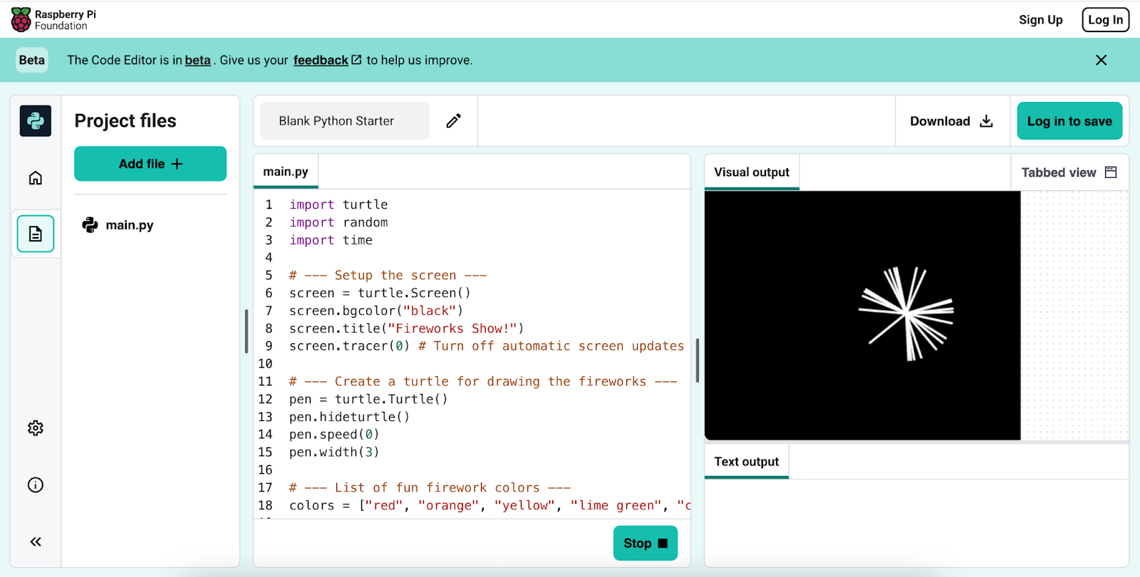
The open-ended structure led to an explosion of creativity and problem-solving.
Without step-by-step instructions, students had to independently explore solutions to questions like:
Some students created multi-file Python projects, separating the logic controlling how the quiz worked from the content, or static information. For example, some students created one file to store the player’s answers and another file to manage the quiz interface and score logic. Students also created other advanced features:
All students met the base requirements, but the open-ended nature of the project allowed more advanced students to push the boundaries, without the need for additional scaffolding.
“They couldn’t just Google the answer; they had to think critically and test ideas. That’s what made it powerful.”
Mr Mason noted that the project’s success was due in large part to the flexibility and responsiveness of the Code Editor. Students could iterate quickly, test their ideas, and collaborate, all within a platform built for classroom coding.
“It was the most successful thing I’ve done. I’ll definitely be doing it again every year.”
Join St Joseph’s College and the 1300+ other schools helping their students build a strong foundation in text-based programming with the Code Editor for Education.
The post Fostering creativity through open-ended projects with Code Editor for Education appeared first on Raspberry Pi Foundation.


