Security updates have been issued by Debian (chromium, firefox-esr, and gst-plugins-ugly1.0), Fedora (firefox, libeconf, libwebsockets, mosquitto, and rust-rustls-webpki), SUSE (amazon-ssm-agent, open-vm-tools, and terraform-provider-helm), and Ubuntu (linux-azure, linux-azure, linux-azure-5.15, linux-azure-fde, linux-gcp-5.15, linux-gcp-5.4, linux-oracle-5.4, linux-gkeop, linux-gkeop-5.15, linux-intel-iotg, linux-kvm, linux-oracle, and python-git).
In 2017, AWS announced the release of Rate-based Rules for AWS WAF, a new rule type that helps protect websites and APIs from application-level threats such as distributed denial of service (DDoS) attacks, brute force log-in attempts, and bad bots. Rate-based rules track the rate of requests for each originating IP address and invokes a rule action on IPs with rates that exceed a set limit.
While rate-based rules are useful to detect and mitigate a broad variety of bad actors, threats have evolved to bypass request-rate limit rules. For example, one bypass technique is to send a high volumes of requests by spreading them across thousands of unique IP addresses.
In May 2023, AWS announced AWS WAF enhancements to the existing rate-based rules feature that you can use to create more dynamic and intelligent rules by using additional HTTP request attributes for request rate limiting. For example, you can now choose from the following predefined keys to configure your rules: label namespace, header, cookie, query parameter, query string, HTTP method, URI path and source IP Address or IP Address in a header. Additionally, you can combine up to five composite keys as parameters for stronger rule development. These rule definition enhancements help improve perimeter security measures against sophisticated application-layer DDoS attacks using AWS WAF. For more information about the supported request attributes, see Rate-based rule statement in the AWS WAF Developer Guide.
In this blog post, you will learn more about these new AWS WAF feature enhancements and how you can use alternative request attributes to create more robust and granular sets of rules. In addition, you’ll learn how to combine keys to create a composite aggregation key to uniquely identify a specific combination of elements to improve rate tracking.
Getting started
Configuring advanced rate-based rules is similar to configuring simple rate-based rules. The process starts with creating a new custom rule of type rate-based rule, entering the rate limit value, selecting custom keys, choosing the key from the request aggregation key dropdown menu, and adding additional composite keys by choosing Add a request aggregation key as shown in Figure 1.
Figure 1: Creating an advanced rate-based rule with two aggregation keys
For existing rules, you can update those rate-based rules to use the new functionality by editing them. For example, you can add a header to be aggregated with the source IP address, as shown in Figure 2. Note that previously created rules will not be modified.
Figure 2: Add a second key to an existing rate-based rule
You still can set the same rule action, such as block, count, captcha, or challenge. Optionally, you can continue applying a scope-down statement to limit rule action. For example, you can limit the scope to a certain application path or requests with a specified header. You can scope down the inspection criteria so that only certain requests are counted towards rate limiting, and use certain keys to aggregate those requests together. A technique would be to count only requests that have /api at the start of the URI, and aggregate them based on their SessionId cookie value.
Target use cases
Now that you’re familiar with the foundations of advanced rate-based rules, let’s explore how they can improve your security posture using the following use cases:
Enhanced Application (Layer 7) DDoS protection
Improved API security
Enriched request throttling
Use case 1: Enhance Layer 7 DDoS mitigation
The first use case that you might find beneficial is to enhance Layer 7 DDoS mitigation. An HTTP request flood is the most common vector of DDoS attacks. This attack type aims to affect application availability by exhausting available resources to run the application.
Before the release of these enhancements to AWS WAF rules, rules were limited by aggregating requests based on the IP address from the request origin or configured to use a forwarded IP address in an HTTP header such as X-Forwarded-For. Now you can create a more robust rate-based rule to help protect your web application from DDoS attacks by tracking requests based on a different key or a combination of keys. Let’s examine some examples.
To help detect pervasive bots, such as scrapers, scanners, and crawlers, or common bots that are distributed across many unique IP addresses, a rule can look for static request data like a custom header — for example, User-Agent.
To uniquely identity users behind a NAT gateway, you can use a cookie in addition to an IP address. Before the aggregation keys feature, it was difficult to identify users who connected from a single IP address. Now, you can use the session cookie to aggregate requests by their session identifier and IP address.
Note that for Layer 7 DDoS mitigation, tracking by session ID in cookies can be circumvented, because bots might send random values or not send any cookie at all. It’s a good idea to keep an IP-based blanket rate-limiting rule to block offending IP addresses that reach a certain high rate, regardless of their request attributes. In that case, the keys would look like:
Key 1: Session cookie
Key 2: IP address
You can reduce false positives when using AWS Managed Rules (AMR) IP reputation lists by rate limiting based on their label namespace. Labelling functionality is a powerful feature that allows you to map the requests that match a specific pattern and apply custom rules to them. In this case, you can match the label namespace provided by the AMR IP reputation list that includes AWSManagedIPDDoSList, which is a list of IP addresses that have been identified as actively engaging in DDoS activities.
You might want to be cautious about using this group list in block mode, because there’s a chance of blocking legitimate users. To mitigate this, use the list in count mode and create an advanced rate-based rule to aggregate all requests with the label namespace awswaf:managed:aws:amazon-ip-list:, targeting captcha as the rule action. This lets you reduce false positives without compromising security. Applying captcha as an action for the rule reduces serving captcha to all users and instead only applies it when the rate of requests exceeds the defined limit. The key for this rule would be:
Labels (AMR IP reputation lists).
Use case 2: API security
In this second use case, you learn how to use an advanced rate-based rule to improve the security of an API. Protecting an API with rate-limiting rules helps ensure that requests aren’t being sent too frequently in a short amount of time. Reducing the risk from misusing an API helps to ensure that only legitimate requests are handled and not denied due to an overload of requests.
Now, you can create advanced rate-based rules that track API requests based on two aggregation keys. For example, HTTP method to differentiate between GET, POST, and other requests in combination with a custom header like Authorization to match a JSON Web Token (JWT). JWTs are not decrypted by AWS WAF, and AWS WAF only aggregates requests with the same token. This can help to ensure that a token is not being used maliciously or to bypass rate-limiting rules. An additional benefit of this configuration is that requests with no authorization headers are being aggregated together towards the rate limiting threshold. The keys for this use case are:
Key 1: HTTP method
Key 2: Custom header (Authorization)
In addition, you can configure a rule to block and add a custom response when the requests limit is reached. For example, by returning HTTP error code 429 (too many requests) with a Retry-After header indicating the requester should wait 900 seconds (15 minutes) before making a new request.
There are many situations where throttling should be considered. For example, if you want to maintain the performance of a service API by providing fair usage for all users, you can have different rate limits based on the type or purpose of the API, such as mutable or non-mutable requests. To achieve this, you can create two advanced rate-based rules using aggregation keys like IP address, combined with an HTTP request parameter for either mutable or non-mutable that indicates the type of request. Each rule will have its own HTTP request parameter, and you can set different maximum values for the rate limit. The keys for this use case are:
Key 1: HTTP request parameter
Key 2: IP address
Another example where throttling can be helpful is for a multi-tenant application where you want to track requests made by each tenant’s users. Let’s say you have a free tier but also a paying subscription model for which you want to allow a higher request rate. For this use case, it’s recommended to use two different URI paths to verify that the two tenants are kept separated. Additionally, it is advised to still use a custom header or query string parameter to differentiate between the two tenants, such as a tenant-id header or parameter that contains a unique identifier for each tenant. To implement this type of throttling using advanced rate-based rules, you can create two rules using an IP address in combination with the custom header as aggregation keys. Each rule can have its own maximum value for rate limiting, as well as a scope-down statement that matches requests for each URI path. The keys and scope-down statement for this use case are:
Key 1: Custom header (tenant-id)
Key 2: IP address
Scope down statement (URI path)
As a third example, you can rate-limit web applications based on the total number of requests that can be handled. For this use case, you can use the new Count all as aggregation option. The option counts and rate-limits the requests that match the rule’s scope-down statement, which is required for this type of aggregation. One option is to scope down and inspect the URI path to target a specific functionality like a /history-search page. An option when you need to control how many requests go to a specific domain is to scope down a single header to a specific host, creating one rule for a.example.com and another rule for b.example.com.
Request Aggregation: Count all
Scope down statement (URI path | Single header)
For these examples, you can block with a custom response when the requests exceed the limit. For example, by returning the same HTTP error code and header, but adding a custom response body with a message like “You have reached the maximum number of requests allowed.”
Logging
The AWS WAF logs now include additional information about request keys used for request-rate tracking and the values of matched request keys. In addition to the existing IP or Forwarded_IP values, you can see the updated log fieldslimitKey and customValue, where the limitKey field now shows either CustomKeys for custom aggregate key settings or Constant for count all requests. CustomValues shows an array of keys, names, and values.
Figure 3: Example log output for the advanced rate-based rule showing updated limitKey and customValues fields
As mentioned in the first use case, to get more detailed information about the traffic that’s analyzed by the web ACL, consider enabling logging. If you choose to enable Amazon CloudWatch Logs as the log destination, you can use CloudWatch Logs Insights and advanced queries to interactively search and analyze logs.
For example, you can use the following query to get the request information that matches rate-based rules, including the updated keys and values, directly from the AWS WAF console.
Figure 4 shows the CloudWatch Log Insights query and the logs output including custom keys, names, and values fields.
Figure 4: The CloudWatch Log Insights query and the logs output
Pricing
There is no additional cost for using advanced rate-base rules; standard AWS WAF pricing applies when you use this feature. For AWS WAF pricing information, see AWS WAF Pricing. You only need to be aware that using aggregation keys will increase AWS WAF web ACL capacity units (WCU) usage for the rule. WCU usage is calculated based on how many keys you want to use for rate limiting. The current model of 2 WCUs plus any additional WCUs for a nested statement is being updated to 2 WCUs as a base, and 30 WCUs for each custom aggregation key that you specify. For example, if you want to create aggregation keys with an IP address in combination with a session cookie, this will use 62 WCUs, and aggregation keys with an IP address, session cookie, and customer header will use 92 WCUs. For more details about the WCU-based cost structure, visit Rate-based rule statement in the AWS WAF Developer Guide.
Conclusion
In this blog post, you learned about AWS WAF enhancements to existing rate-based rules that now support request parameters in addition to IP addresses. Additionally, these enhancements allow you to create composite keys based on up to five request parameters. This new capability allows you to be either more coarse in aggregating requests (such as all the requests that have an IP reputation label associated with them) or finer (such as aggregate requests for a specific session ID, not its IP address).
For more rule examples that include JSON rule configuration, visit Rate-based rule examples in the AWS WAF Developer Guide.
If you have feedback about this post, submit comments in the Comments section below. If you have questions about this post, contact AWS Support.
Want more AWS Security news? Follow us on Twitter.
Being able to get real-time information from applications in production is extremely important. Many times software passes local testing and automation, but then users report that something isn’t working correctly. Being able to quickly see what is happening, and how often, is critical to debugging.
This is why we originally developed the Workers Tail feature – to allow developers the ability to view requests, exceptions, and information for their Workers and to provide a window into what’s happening in real time. When we developed it, we also took the opportunity to build it on top of our own Workers technology using products like Trace Workers and Durable Objects. Over the last couple of years, we’ve continued to iterate on this feature – allowing users to quickly access logs from the Dashboard and via Wrangler CLI.
Today, we’re excited to announce that tail can now be enabled for Workers at any size and scale! In addition to telling you about the new and improved scalability, we wanted to share how we built it, and the changes we made to enable it to scale better.
Why Tail was limited
Tail leverages Durable Objects to handle coordination between the Worker producing messages and consumers like wrangler and the Cloudflare dashboard, and Durable Objects are a great choice for handling real-time communication like this. However, when a single Durable Object instance starts to receive a very high volume of traffic – like the kind that can come with tailing live Workers – it can see some performance issues.
As a result, Workers with a high volume of traffic could not be supported by the original Tail infrastructure. Tail had to be limited to Workers receiving 100 requests/second (RPS) or less. This was a significant limitation that resulted in many users with large, high-traffic Workers having to turn to their own tooling to get proper observability in production.
Believing that every feature we provide should scale with users during their development journey, we set out to improve Tail's performance at high loads.
Updating the way filters work
The first improvement was to the existing filtering feature. When starting a Tail with wrangler tail (and now with the Cloudflare dashboard) users have the ability to filter out messages based on information in the requests or logs. Previously, this filtering was handled within the Durable Object, which meant that even if a user was filtering out the majority of their traffic, the Durable Object would still have to handle every message. Often users with high traffic Tails were using many filters to better interpret their logs, but wouldn’t be able to start a Tail due to the 100 RPS limit.
We moved filtering out of the Durable Object and into the Tail message producer, preventing any filtered messages from reaching the Tail Durable Object, and thereby reducing the load on the Tail Durable Object. Moving the filtering out of the Durable Object was the first step in improving Tail’s performance at scale.
Sampling logs to keep Tails within Durable Object limits
After moving log filtering outside of the Durable Object, there was still the issue of determining when Tails could be started since there was no way to determine to what degree filters would reduce traffic for a given Tail, and simply starting a Durable Object back up would mean that it more than likely hit the 100 RPS limit immediately.
The solution for this was to add a safety mechanism for the Durable Object while the Tail was running.
We created a simple controller to track the RPS hitting a Durable Object and sample messages until the desired volume of 100 RPS is reached. As shown below, sampling keeps the Tail Durable Object RPS below the target of 100.
When messages are sampled, the following message appears every five seconds to let the user know that they are in sampling mode:
This message goes away once the Tail is stopped or filters are applied that drop the RPS below 100.
A final failsafe
Finally as a last resort a failsafe mechanism was added in the case the Durable Object gets fully overloaded. Since RPS tracking is done within the Durable Object, if the Durable Object is overloaded due to an extremely large amount of traffic, the sampling mechanism will fail.
In the case that an overload is detected, all messages forwarded to the Durable Object are stopped periodically to prevent any issues with Workers infrastructure.
Here we can see a user who had a large amount of traffic that started to become sampled. As the traffic increased, the number of sampled messages grew. Since the traffic was too fast for the sampling mechanism to handle, the Durable Object got overloaded. However, soon excess messages were blocked and the overload stopped.
Try it out
These new improvements are in place currently and available to all users 🎉
To Tail Workers via the Dashboard, log in, navigate to your Worker, and click on the Logs tab. You can then start a log stream via the default view.
If you’re using the Wrangler CLI, you can start a new Tail by running wrangler tail.
Beyond Worker tail
While we're excited for tail to be able to reach new limits and scale, we also recognize users may want to go beyond the live logs provided by Tail.
For example, if you’d like to push log events to additional destinations for a historical view of your application’s performance, we offer Logpush. If you’d like more insight into and control over log messages and events themselves, we offer Tail Workers.
These products, and others, can be read about in our Logs documentation. All of them are available for use today.
As competition grows fiercer, marketers need ways to ensure they reach each user with personalized content on their most critical channels. Short message/messaging service (SMS) is a key part of that effort, touching more than 5 billion people worldwide, with an impressive 82% open rate. However, SMS lacks the built-in engagement metrics supported by other channels.
To bridge this gap, leading customer engagement platform, Braze, recently built an in-house SMS link shortening solution using Amazon DynamoDB and Amazon DynamoDB Accelerator (DAX). It’s designed to handle up to 27 billion redirects per month, allowing marketers to automatically shorten SMS-related URLs. Alongside the Braze Intelligence Suite, you can use SMS click data in reporting functions and retargeting actions. Read on to learn how Braze created this feature and the impact it’s having on marketers and consumers alike.
SMS link shortening approach
Many Braze customers have used third-party SMS link shortening solutions in the past. However, this approach complicates the SMS composition process and isolates click metrics from Braze analytics. This makes it difficult to get a full picture of SMS performance.
Figure 1. Multiple approaches for shortening URLs
The following table compares all 3 approaches for their pros and cons.
Scenario
#1 – Unshortened URL in SMS
#2 – 3rd Party Shortener
#3 – Braze Link Shortening & Click Tracking
Low Character Count
X
✓
✓
Total Clicks
X
✓
✓
Ability to Retarget Users
X
X
✓
Ability to Trigger Subsequent Messages
X
X
✓
With link shortening built in-house and more tightly integrated into the Braze platform, Braze can maintain more control over their roadmap priority. By developing the tool internally, Braze achieved a 90% reduction in ongoing expenses compared with the $400,000 annual expense associated with using an outside solution.
Braze SMS link shortening: Flow and architecture
Figure 2. SMS link shortening architecture
The following steps explain the link shortening architecture:
First, customers initiate campaigns via the Braze Dashboard. Using this interface, they can also make requests to shorten URLs.
The URL registration process is managed by a Kubernetes-deployed Go-based service. This service not only shortens the provided URL but also maintains reference data in Amazon DynamoDB.
After processing, the dashboard receives the generated campaign details alongside the shortened URL.
The fully refined campaign can be efficiently distributed to intended recipients through SMS channels.
Upon a user’s interaction with the shortened URL, the message gets directed to the URL redirect service. This redirection occurs through an Application Load Balancer.
The redirect service processes links in messages, calls the service, and replaces links before sending to carriers.
Asynchronous calls feed data to a Kafka queue for metrics, using the HTTP sink connector integrated with Braze systems.
The registration and redirect services are decoupled from the Braze platform to enable independent deployment and scaling due to different requirements. Both the services are running the same code, but with different endpoints exposed, depending on the functionality of a given Kubernetes pod. This restricts internal access to the registration endpoint and permits independent scaling of the services, while still maintaining a fast response time.
Braze SMS link shortening: Scale
Right now, our customers use the Braze platform to send about 200 million SMS messages each month, with peak speeds of around 2,000 messages per second. Many of these messages contain one or more URLs that need to be shortened. In order to support the scalability of the link shortening feature and give us room to grow, we designed the service to handle 33 million URLs sent per month, and 3.25 million redirects per month. We assumed that we’d see up to 65 million database writes per month and 3.25 million reads per month in connection with the redirect service. This would require storage of 65 GB per month, with peaks of ~2,000 writes and 100 reads per second.
With these needs in mind, we carried out testing and determined that Amazon DynamoDB made the most sense as the backend database for the redirect service. To determine this, we tested read and write performance and found that it exceeded our needs. Additionally, it was fully managed, thus requiring less maintenance expertise, and included DAX out of the box. Most clicks happen close to send, so leveraging DAX helps us smooth out the read and write load associated with the SMS link shortener.
Because we know how long we must keep the relevant written elements at write time, we’re able to use DynamoDB Time to Live (TTL) to effectively manage their lifecycle. Finally, we’re careful to evenly distribute partition keys to avoid hot partitions, and DynamoDB’s autoscaling capabilities make it possible for us to respond more efficiently to spikes in demand.
Braze SMS link shortening: Flow
Figure 3. Braze SMS link shortening flow
When the marketer initiates an SMS send, Braze checks its primary datastore (a MongoDB collection) to see if the link has already been shortened (see Figure 3). If it has, Braze re-uses that shortened link and continues the send. If it hasn’t, the registration process is initiated to generate a new site identifier that encodes the generation date and saves campaign information in DynamoDB via DAX.
The response from the registration service is used to generate a short link (1a) for the SMS.
A recipient gets an SMS containing a short link (2).
Recipient decides to tap it (3). Braze smoothly redirects them to the destination URL, and updates the campaign statistics to show that the link was tapped.
Using Amazon Route 53’s latency-based routing, Braze directs the recipient to the nearest endpoint (Braze currently has North America and EU deployments), then inspects the link to ensure validity and that it hasn’t expired. If it passes those checks, the redirect service queries DynamoDB via DAX for information about the redirect (3a). Initial redirects are cached at send time, while later requests query the DAX cache.
The user is redirected with a P99 redirect latency of less than 10 milliseconds (3b).
Emit campaign-level metrics on redirects.
Braze generates URL identifiers, which serve as the partition key to the DynamoDB collection, by generating a random number. We concatenate the generation date timestamp to the number, then Base66 encode the value. This results in a generated URL that looks like https://brz.ai/5xRmz, with “5xRmz” being the encoded URL identifier. The use of randomized partition keys helps avoid hot, overloaded partitions. Embedding the generation date lets us see when a given link was generated without querying the database. This helps us maintain performance and reduce costs by removing old links from the database. Other cost control measures include autoscaling and the use of DAX to avoid repeat reads of the same data. We also query DynamoDB directly against a hash key, avoiding scatter-gather queries.
Braze link shortening feature results
Since its launch, SMS link shortening has been used by over 300 Braze customer companies in more than 700 million SMS messages. This includes 50% of the total SMS volume sent by Braze during last year’s Black Friday period. There has been a tangible reduction in the time it takes to build and send SMS. “The Motley Fool”, a financial media company, saved up to four hours of work per month while driving click rates of up to 15%. Another Braze client utilized multimedia messaging service (MMS) and link shortening to encourage users to shop during their “Smart Investment” campaign, rewarding users with additional store credit. Using the engagement data collected with Braze link shortening, they were able to offer engaged users unique messaging and follow-up offers. They retargeted users who did not interact with the message via other Braze messaging channels.
Conclusion
The Braze platform is designed to be both accessible to marketers and capable of supporting best-in-class cross-channel customer engagement. Our SMS link shortening feature, supported by AWS, enables marketers to provide an exceptional user experience and save time and money.
A Brazilian spyware app vendor was hacked by activists:
In an undated note seen by TechCrunch, the unnamed hackers described how they found and exploited several security vulnerabilities that allowed them to compromise WebDetetive’s servers and access its user databases. By exploiting other flaws in the spyware maker’s web dashboard—used by abusers to access the stolen phone data of their victims—the hackers said they enumerated and downloaded every dashboard record, including every customer’s email address.
The hackers said that dashboard access also allowed them to delete victim devices from the spyware network altogether, effectively severing the connection at the server level to prevent the device from uploading new data. “Which we definitely did. Because we could. Because #fuckstalkerware,” the hackers wrote in the note.
The note was included in a cache containing more than 1.5 gigabytes of data scraped from the spyware’s web dashboard. That data included information about each customer, such as the IP address they logged in from and their purchase history. The data also listed every device that each customer had compromised, which version of the spyware the phone was running, and the types of data that the spyware was collecting from the victim’s phone.
PromCon Europe is the eighth conference fully dedicated to the Prometheus monitoring system
Berlin, Germany – September 1, 2023 – The CNCF and the Prometheus team, released the two-day schedule for the single-track PromCon Europe 2023 conference happening in Berlin, Germany from September 28 to September 29, 2023. Attendees will be able to choose from 21 full-length (25min) sessions and up to 20 five-minute lightning talk sessions spanning diverse topics related to Prometheus.
Now in its 8th installment, PromCon brings together Prometheus users and developers from around the world to exchange knowledge, best practices, and experience gained through using Prometheus. The program committee reviewed 66 submissions that will provide a fresh and informative look into the most pressing topics around Prometheus today.
“We are super excited for PromCon to be coming home to Berlin. Prometheus was started in Berlin at Soundcloud in 2012. The first PromCon was hosted in Berlin and in between moved to Munich. This year we’re hosting around 300 attendees at Radialsystem in Friedrichshain, Berlin. Berlin has a vibrant Prometheus community and many of the Prometheus team members live in the neighborhood. It is a great opportunity to network and connect with the Prometheus family who are all passionate about systems and service monitoring,” said Matthias Loibl, Senior Software Engineer at Polar Signals and Prometheus team member who leads this year’s PromCon program committee. “It will be a great event to learn about the latest developments from the Prometheus team itself and connect to some big-scale users of Prometheus up close.”
The community-curated schedule will feature sessions from open source community members, including:
For the full PromCon Europe 2023 program, please visit the schedule.
Registration
Register for the in-person standard pricing of $350 USD through September 25. The venue has space for 300 attendees so don’t wait!
Thank You to Our Sponsors
PromCon Europe 2023 has been made possible thanks to the amazing community around Prometheus and support from our Diamond Sponsor Grafana Labs, Platinum Sponsor Red Hat as well as many more Gold, and Startup sponsors. This year’s edition is organized by Polar Signals and CNCF.
Recently, Rapid7 observed the Fake Browser Update lure tricking users into executing malicious binaries. While analyzing the dropped binaries, Rapid7 determined a new loader is utilized in order to execute infostealers on compromised systems including StealC and Lumma.
The IDAT loader is a new, sophisticated loader that Rapid7 first spotted in July 2023. In earlier versions of the loader, it was disguised as a 7-zip installer that delivered the SecTop RAT. Rapid7 has now observed the loader used to deliver infostealers like Stealc, Lumma, and Amadey. It implements several evasion techniques including Process Doppelgänging, DLL Search Order Hijacking, and Heaven’s Gate. IDAT loader got its name as the threat actor stores the malicious payload in the IDAT chunk of PNG file format.
Prior to this technique, Rapid7 observed threat actors behind the lure utilizing malicious JavaScript files to either reach out to Command and Control (C2) servers or drop the Net Support Remote Access Trojan (RAT).
The following analysis covers the entire attack flow, which starts from the SocGholish malware and ends with the stolen information in threat actors’ hands.
Technical Analysis
Threat Actors (TAs) are often staging their attacks in the way security tools will not detect them and security researchers will have a hard time investigating them.
Figure 1 – Attack Flow
Stage 1 – SocGholish
First observed in the wild as early as 2018, SocGholish was attributed to TA569. Mainly recognized for its initial infection method characterized as “drive-by” downloads, this attack technique involves the injection of malicious JavaScript into compromised yet otherwise legitimate websites. When an unsuspecting individual receives an email with a link to a compromised website and clicks on it, the injected JavaScript will activate as soon as the browser loads the page.
The injected JavaScript investigated by Rapid7 loads an additional JavaScript that will access the final URL when all the following browser conditions are met:
The access originated from the Windows OS
The access originated from an external source
Cookie checks are passed
Figure 2 – Obfuscated JavaScript Embedded in the Compromised Domain
This prompt falsely presents itself as a browser update, with the added layer of credibility coming from the fact that it appears to originate from the intended domain.
Figure 3 – Pop-up Prompting the User to Update their Browser
Once the user interacts with the “Update Chrome” button, the browser is redirected to another URL where a binary automatically downloads to the user’s default download folder. After the user double clicks the fake update binary, it will proceed to download the next stage payload. In this investigation, Rapid7 identified a binary called ChromeSetup.exe, the file name widely used in previous SocGholish attacks.
Stage 2 – MSI Downloader
ChromeSetup.exe downloads and executes the Microsoft Software Installer (MSI) package from: hxxps://ocmtancmi2c5t[.]xyz/82z2fn2afo/b3/update[.]msi.
In similar investigations, Rapid7 observed that the initial dropper executable appearance and file name may vary depending on the user’s browser when visiting the compromised web page. In all instances, the executables contained invalid signatures and attempted to download and install an MSI package.
Rapid7 determined that the MSI package executed with several switches intended to avoid detection:
/qn to avoid an installation UI
/quiet to prevent user interaction
/norestart to prevent the system from restarting during the infection process
When executed, the MSI dropper will write a legitimate VMwareHostOpen.exe executable, multiple legitimate dependencies, and the malicious Dynamic-Link Library (DLL) file vmtools.dll. It will also drop an encrypted vmo.log file which has a PNG file structure and is later decrypted by the malicious DLL. Rapid7 spotted an additional version of the attack where the MSI dropped a legitimate pythonw.exe, legitimate dependencies, and the malicious DLL file python311.dll.In that case, the encrypted file was named pz.log,though the execution flow remains the same.
Figure 4 – Content of vmo.log
Stage 3 – Decryptor
When executed, the legitimate VMWareHostOpen.exe loads the malicious vmtools.dllfrom the same directory as from which the VMWareHostOpen.exeis executed. This technique is known as DLL Search Order Hijacking.
During the execution of vmtools.dll, Rapid7 observed that the DLL loads API libraries from kernel32.dll and ntdll.dll using API hashing and maps them to memory. After the API functions are mapped to memory, the DLL reads the hex string 83 59 EB ED 50 60 E8 and decrypts it using a bitwise XOR operation with the key F5 34 84 C3 3C 0F 8F, revealing the string vmo.log. The file is similar to the Vmo\log directory, where Vmware logs are stored.
The DLL then reads the contents from vmo.log into memory and searches for the string …IDAT. The DLL takes 4 bytes following …IDAT and compares them to the hex values of C6 A5 79 EA. If the 4 bytes following …IDAT are equal to the hex values C6 A5 79 EA, the DLL proceeds to copy all the contents following …IDAT into memory.
Figure 5 – Function Searching for Hex Values C6 A5 79 EA
Once all the data is copied into memory, the DLL attempts to decrypt the copied data using the bitwise XOR operation with key F4 B4 07 9A. Upon additional analysis of other samples, Rapid7 determined that the XOR keys were always stored as 4 bytes following the hex string C6 A5 79 EA.
Figure 6 – XOR Keys found within PNG Files pz.log and vmo.log
Once the DLL decrypts the data in memory, it is decompressed using the RTLDecompressBuffer function. The parameters passed to the function include:
Compression format
Size of compressed data
Size of compressed buffer
Size of uncompressed data
Size of uncompressed buffer
Figure 7 – Parameters passed to RTLDecompressBuffer function
The vmtools.dll DLL utilizes the compression algorithm LZNT1 in order to decompress the decrypted data from the vmo.log file.
After the data is decompressed, the DLL loads mshtml.dll into memory and overwrites its .text section with the decompressed code. After the overwrite, vmtools.dll calls the decompressed code.
Stage 4 – IDAT Injector
Similarly to vmtools.dll,IDAT loader uses dynamic imports. The IDAT injector then expands the %APPDATA% environment variable by using the ExpandEnvironmentStringsW API call. It creates a new folder under %APPDATA%, naming it based on the QueryPerformanceCounter API call output and randomizing its value.
All the dropped files by MSI are copied to the newly created folder. IDAT then creates a new instance of VMWareHostOpen.exefrom the %APPDATA% by using CreateProcessW and exits.
The second instance of VMWareHostOpen.exebehaves the same up until the stage where the IDAT injector code is called from mshtml.dllmemory space. IDAT immediately started the implementation of the Heaven’s Gate evasion technique, which it uses for most API calls until the load of the infostealer is completed.
Heaven’s Gate is widely used by threat actors to evade security tools. It refers to a method for executing a 64-bit process within a 32-bit process or vice versa, allowing a 32-bit process to run in a 64-bit process. This is accomplished by initiating a call or jump instruction through the use of a reserved selector. The key points in analyzing this technique in our case is to change the process mode from 32-bit to 64-bit, the specification of the selector “0x0033” required and followed by the execution of a far call or far jump, as shown in Figure 8.
Figure 8 – Heaven’s Gate technique implementation
The IDAT injector then expands the %TEMP% environment variable by using the ExpandEnvironmentStringsW API call. It creates a string based on the QueryPerformanceCounter API call output and randomizes its value.
Next, the IDAT loader gets the computer name by calling GetComputerNameW API call, and the output is randomized by using randand srand API calls. It uses that randomized value to set a new environment variable by using SetEnvironmentVariableW.This variable is set to a combination of %TEMP% path with the randomized string created previously.
Figure 9 – New Environment variable – TCBEDOPKVDTUFUSOCPTRQFD set to %TEMP%\89680228
Now, the new cmd.exe process is executed by the loader. The loader then creates and writes to the %TEMP%\89680228 file.
Creates a new memory section inside the remote process by using the NtCreateSection API call
Maps a view of the newly created section to the local malicious process with RW protection by using NtMapViewOfSection API call
Maps a view of the previously created section to a remote target process with RX protection by using NtMapViewOfSection API call
Fills the view mapped in the local process with shellcode by using NtWriteVirtualMemory API call
In our case, IDAT loader suspends the main thread on the cmd.exeprocess by using NtSuspendThread API call and then resumes the thread by using NtResumeThreadAPI call After completing the injection, the second instance of VMWareHostOpen.exeexits.
Stage 5 – IDAT Loader:
The injected loader code implements the Heaven’s Gate evasion technique in exactly the same way as the IDAT injector did. It retrieves the TCBEDOPKVDTUFUSOCPTRQFD environment variable, and reads the %TEMP%\89680228 file data into the memory. The data is then recursively XORed with the 3D ED C0 D3 key.
The decrypted data seems to contain configuration data, including which process the infostealer should be loaded, which API calls should be dynamically retrieved, additional code,and more. The loader then deletes the initial malicious DLL (vmtools.dll) by using DeleteFileW.The loader finally injects the infostealer code into the explorer.exe process by using the Process Doppelgänging injection technique.
TheProcess Doppelgängingmethod utilizes the Transactional NTFS feature within the Windows operating system. This feature is designed to ensure data integrity in the event of unexpected errors. For instance, when an application needs to write or modify a file, there’s a risk of data corruption if an error occurs during the write process. To prevent such issues, an application can open the file in a transactional mode to perform the modification and then commit the modification, thereby preventing any potential corruption. The modification either succeeds entirely or does not commence.
Process Doppelgänging exploits this feature to replace a legitimate file with a malicious one, leading to a process injection. The malicious file is created within a transaction, then committed to the legitimate file, and subsequently executed. The Process Doppelgängingin our sample was performed by:
Initiating a transaction by using NtCreateTransaction API call
Creating a new file by using NtCreateFile API call
Writing to the new file by using NtWriteFileAPI call
Writing malicious code into a section of the local process using NtCreateSectionAPI call
Discarding the transaction by using NtRollbackTransactionAPI call
Running a new instance of explorer.exe process by using NtCreateProcessEx API call
Running the malicious code inside explorer.exe process by using NtCreateThreadExAPI call
If the file created within a transaction is rolled back (instead of committed), but the file section was already mapped into the process memory, the process injection will still be performed.
The final payload injected into the explorer.exe process was identified by Rapid7 as Lumma Stealer.
Figure 10 – Process Tree
Throughout the whole attack flow, the malware delays execution by using NtDelayExecution, a technique that is usually used to escape sandboxes.
As previously mentioned, Rapid7 has investigated several IDAT loader samples. The main differences were:
The legitimate software that loads the malicious DLL.
The name of the staging directory created within %APPDATA%.
The process the IDAT injector injects the Loader code to.
The process into which the infostealer/RAT loaded into.
Rapid7 observed the IDAT loader has been used to load the following infostealers and RAT: Stealc, Lumma and Amadey infostealers and SecTop RAT.
Figure 11 – Part of an HTTP POST request to a StealC C2 domainFigure 12 – An HTTP POST request to a Lumma Stealer C2 domain
Conclusion
IDAT Loader is a new sophisticated loader that utilizes multiple evasion techniques in order to execute various commodity malware including InfoStealers and RAT’s. The Threat Actors behind the Fake Update campaign have been packaging the IDAT Loader into DLLs that are loaded by legitimate programs such as VMWarehost, Python and Windows Defender.
Rapid7 Customers
For Rapid7 MDR and InsightIDR customers, the following Attacker Behavior Analytics (ABA) rules are currently deployed and alerting on the activity described in this blog:
Attacker Technique – MSIExec loading object via HTTP
Suspicious Process – FSUtil Zeroing Out a File
Suspicious Process – Users Script Spawns Cmd And Redirects Output To Temp File
Suspicious Process – Possible Dropper Script Executed From Users Downloads Directory
Suspicious Process – WScript Runs JavaScript File from Temp Or Download Directory
MITRE ATT&CK Techniques:
Initial Access
Drive-by Compromise (T1189)
The SocGholish Uses Drive-by Compromise technique to target user’s web browser
Defense Evasion
System Binary Proxy Execution: Msiexec (T1218.007)
The ChromeSetup.exe downloader (C9094685AE4851FD5A5B886B73C7B07EFD9B47EA0BDAE3F823D035CF1B3B9E48) downloads and executes .msi file
Execution
User Execution: Malicious File (T1204.002)
Update.msi (53C3982F452E570DB6599E004D196A8A3B8399C9D484F78CDB481C2703138D47) drops and executes VMWareHostOpen.exe
Defense Evasion
Hijack Execution Flow: DLL Search Order Hijacking (T1574.001)
VMWareHostOpen.exe loads a malicious vmtools.dll (931D78C733C6287CEC991659ED16513862BFC6F5E42B74A8A82E4FA6C8A3FE06)
Ingesting a high volume of streaming data has been a defining characteristic of operational analytics workloads with Amazon OpenSearch Service. Many of these workloads involve either self-managed Apache Kafka or Amazon Managed Streaming for Apache Kafka (Amazon MSK) to satisfy their data streaming needs. Consuming data from Amazon MSK and writing to OpenSearch Service has been a challenge for customers. AWS Lambda, custom code, Kafka Connect, and Logstash have been used for ingesting this data. These methods involve tools that must be built and maintained. In this post, we introduce Amazon MSK as a source to Amazon OpenSearch Ingestion, a serverless, fully managed, real-time data collector for OpenSearch Service that makes this ingestion even easier.
Solution overview
The following diagram shows the flow from data sources to Amazon OpenSearch Service.
The flow contains the following steps:
Data sources produce data and send that data to Amazon MSK
OpenSearch Ingestion consumes the data from Amazon MSK.
OpenSearch Ingestion transforms, enriches, and writes the data into OpenSearch Service.
Users search, explore, and analyze the data with OpenSearch Dashboards.
Prerequisites
You will need a provisioned MSK cluster created with appropriate data sources. The sources, as producers, write data into Amazon MSK. The cluster should be created with the appropriate Availability Zone, storage, compute, security and other configurations to suit your workload needs. To provision your MSK cluster and have your sources producing data, see Getting started using Amazon MSK.
As of this writing, OpenSearch Ingestion supports Amazon MSK provisioned, but not Amazon MSK Serverless. However, OpenSearch Ingestion can reside in the same or different account where Amazon MSK is present. OpenSearch Ingestion uses AWS PrivateLink to read data, so you must turn on multi-VPC connectivity on your MSK cluster. For more information, see Amazon MSK multi-VPC private connectivity in a single Region. OpenSearch Ingestion can write data to Amazon Simple Storage Service (Amazon S3), provisioned OpenSearch Service, and Amazon OpenSearch Service. In this solution, we use a provisioned OpenSearch Service domain as a sink for OSI. Refer to Getting started with Amazon OpenSearch Service to create a provisioned OpenSearch Service domain. You will need appropriate permission to read data from Amazon MSK and write data to OpenSearch Service. The following sections outline the required permissions.
Permissions required
To read from Amazon MSK and write to Amazon OpenSearch Service, you need to create a an AWS Identity and Access Management (IAM) role used by Amazon OpenSearch Ingestion. In this post we use a role called pipeline-Role for this purpose. To create this role please see Creating IAM roles.
Reading from Amazon MSK
OpenSearch Ingestion will need permission to create a PrivateLink connection and other actions that can be performed on your MSK cluster. Edit your MSK cluster policy to include the following snippet with appropriate permissions. If your OpenSearch Ingestion pipeline resides in an account different from your MSK cluster, you will need a second section to allow this pipeline. Use proper semantic conventions when providing the cluster, topic, and group permissions and remove the comments from the policy before using.
{
  "Version": "2012-10-17",
  "Statement": [
    {
      "Effect": "Allow",
      "Principal": {
        "Service": "osis-pipelines.aws.internal"
      },
      "Action": [
        "kafka:CreateVpcConnection",
        "kafka:GetBootstrapBrokers",
        "kafka:DescribeCluster"
      ],
      # Change this to your msk arn
      "Resource": "arn:aws:kafka:us-east-1:XXXXXXXXXXXX:cluster/test-cluster/xxxxxxxx-xxxx-xx"
    },
    ### Following permissions are required if msk cluster is in different account than osi pipeline
    {
      "Effect": "Allow",
      "Principal": {
        # Change this to your sts role arn used in the pipeline
        "AWS": "arn:aws:iam:: XXXXXXXXXXXX:role/PipelineRole"
      },
      "Action": [
        "kafka-cluster:*",
        "kafka:*"
      ],
      "Resource": [
        # Change this to your msk arn
        "arn:aws:kafka:us-east-1: XXXXXXXXXXXX:cluster/test-cluster/xxxxxxxx-xxxx-xx",
        # Change this as per your cluster name & kafka topic name
        "arn:aws:kafka:us-east-1: XXXXXXXXXXXX:topic/test-cluster/xxxxxxxx-xxxx-xx/*",
        # Change this as per your cluster name
        "arn:aws:kafka:us-east-1: XXXXXXXXXXXX:group/test-cluster/*"
      ]
    }
  ]
}
Edit the pipeline role’s inline policy to include the following permissions. Ensure that you have removed the comments before using the policy.
{
    "Version": "2012-10-17",
    "Statement": [
        {
            "Effect": "Allow",
            "Action": [
                "kafka-cluster:Connect",
                "kafka-cluster:AlterCluster",
                "kafka-cluster:DescribeCluster",
                "kafka:DescribeClusterV2",
                "kafka:GetBootstrapBrokers"
            ],
            "Resource": [
                # Change this to your msk arn
                "arn:aws:kafka:us-east-1:XXXXXXXXXXXX:cluster/test-cluster/xxxxxxxx-xxxx-xx"
            ]
        },
        {
            "Effect": "Allow",
            "Action": [
                "kafka-cluster:*Topic*",
                "kafka-cluster:ReadData"
            ],
            "Resource": [
                # Change this to your kafka topic and cluster name
                "arn:aws:kafka:us-east-1: XXXXXXXXXXXX:topic/test-cluster/xxxxxxxx-xxxx-xx/topic-to-consume"
            ]
        },
        {
            "Effect": "Allow",
            "Action": [
                "kafka-cluster:AlterGroup",
                "kafka-cluster:DescribeGroup"
            ],
            "Resource": [
                # change this as per your cluster name
                "arn:aws:kafka:us-east-1: XXXXXXXXXXXX:group/test-cluster/*"
            ]
        }
    ]
}
Writing to OpenSearch Service
In this section, you provide the pipeline role with necessary permissions to write to OpenSearch Service. As a best practice, we recommend using fine-grained access control in OpenSearch Service. Use OpenSearch dashboards to map a pipeline role to an appropriate backend role. For more information on mapping roles to users, see Managing permissions. For example, all_access is a built-in role that grants administrative permission to all OpenSearch functions. When deploying to a production environment, ensure that you use a role with enough permissions to write to your OpenSearch domain.
Creating OpenSearch Ingestion pipelines
The pipeline role now has the correct set of permissions to read from Amazon MSK and write to OpenSearch Service. Navigate to the OpenSearch Service console, choose Pipelines, then choose Create pipeline.
Choose a suitable name for the pipeline. and se the pipeline capacity with appropriate minimum and maximum OpenSearch Compute Unit (OCU). Then choose ‘AWS-MSKPipeline’ from the dropdown menu as shown below.
Use the provided template to fill in all the required fields. The snippet in the following section shows the fields that needs to be filled in red.
Configuring Amazon MSK source
The following sample configuration snippet shows every setting you need to get the pipeline running:
msk-pipeline:
  source:
    kafka:
      acknowledgments: true                     # Default is false
      topics:
         - name: "<topic name>"
           group_id: "<consumer group id>"
           serde_format: json                   # Remove, if Schema Registry is used. (Other option is plaintext)

           # Below defaults can be tuned as needed
           # fetch_max_bytes: 52428800          Optional
           # fetch_max_wait: 500                Optional (in msecs)
           # fetch_min_bytes: 1                 Optional (in MB)
           # max_partition_fetch_bytes: 1048576 Optional
           # consumer_max_poll_records: 500     Optional
           # auto_offset_reset: "earliest"      Optional (other option is "earliest")
           # key_mode: include_as_field         Optional (other options are include_as_field, discard)


           serde_format: json                   # Remove, if Schema Registry is used. (Other option is plaintext)

      # Enable this configuration if Glue schema registry is used
      # schema:
      #   type: aws_glue

      aws:
        # Provide the Role ARN with access to MSK. This role should have a trust relationship with osis-pipelines.amazonaws.com
        # sts_role_arn: "arn:aws:iam::XXXXXXXXXXXX:role/Example-Role"
        # Provide the region of the domain.
        # region: "us-west-2"
        msk:
          # Provide the MSK ARN.
          arn: "arn:aws:kafka:us-west-2:XXXXXXXXXXXX:cluster/msk-prov-1/id"

  sink:
      - opensearch:
          # Provide an AWS OpenSearch Service domain endpoint
          # hosts: [ "https://search-mydomain-1a2a3a4a5a6a7a8a9a0a9a8a7a.us-east-1.es.amazonaws.com" ]
          aws:
          # Provide a Role ARN with access to the domain. This role should have a trust relationship with osis-pipelines.amazonaws.com
          # sts_role_arn: "arn:aws:iam::XXXXXXXXXXXX:role/Example-Role"
          # Provide the region of the domain.
          # region: "us-east-1"
          # Enable the 'serverless' flag if the sink is an Amazon OpenSearch Serverless collection
          # serverless: true
          # index name can be auto-generated from topic name
          index: "index_${getMetadata(\"kafka_topic\")}-%{yyyy.MM.dd}"
          # Enable 'distribution_version' setting if the AWS OpenSearch Service domain is of version Elasticsearch 6.x
          # distribution_version: "es6"
          # Enable the S3 DLQ to capture any failed requests in Ohan S3 bucket
          # dlq:
            # s3:
            # Provide an S3 bucket
We use the following parameters:
acknowledgements – Set to true for OpenSearch Ingestion to ensure that the data is delivered to the sinks before committing the offsets in Amazon MSK. The default value is set to false.
name – This specifies topic OpenSearch Ingestion can read from. You can read a maximum of four topics per pipeline.
group_id – This parameter specifies that the pipeline is part of the consumer group. With this setting, a single consumer group can be scaled to as many pipelines as needed for very high throughput.
serde_format – Specifies a deserialization method to be used for the data read from Amazon MSK. The options are JSON and plaintext.
AWS sts_role_arn and OpenSearch sts_role_arn – Specifies the role OpenSearch Ingestion uses for reading and writing. Specify the ARN of the role you created from the last section. OpenSearch Ingestion currently uses the same role for reading and writing.
MSK arn – Specifies the MSK cluster to consume data from.
OpenSearch host and index – Specifies the OpenSearch domain URL and where the index should write.
When you have configured the Kafka source, choose the network access type and log publishing options. Public pipelines do not involve PrivateLink and they will not incur a cost associated with PrivateLink. Choose Next and review all configurations. When you are satisfied, choose Create pipeline.
Log in to OpenSearch Dashboards to see your indexes and search the data.
Recommended compute units (OCUs) for the MSK pipeline
Each compute unit has one consumer per topic. Brokers will balance partitions among these consumers for a given topic. However, when the number of partitions is greater than the number of consumers, Amazon MSK will host multiple partitions on every consumer. OpenSearch Ingestion has built-in auto scaling to scale up or down based on CPU usage or number of pending records in the pipeline. For optimal performance, partitions should be distributed across many compute units for parallel processing. If topics have a large number of partitions, for example, more than 96 (maximum OCUs per pipeline), we recommend configuring a pipeline with 1–96 OCUs because it will auto scale as needed. If a topic has a low number of partitions, for example, less than 96, then keep the maximum compute unit to same as the number of partitions. When pipeline has more than one topic, user can pick a topic with highest number of partitions as a reference to configure maximum computes units. By adding another pipeline with a new set of OCUs to the same topic and consumer group, you can scale the throughput almost linearly.
Clean up
To avoid future charges, clean up any unused resources from your AWS account.
Conclusion
In this post, you saw how to use Amazon MSK as a source for OpenSearch Ingestion. This not only addresses the ease of data consumption from Amazon MSK, but it also relieves you of the burden of self-managing and manually scaling consumers for varying and unpredictable high-speed, streaming operational analytics data. Please refer to the ‘sources’ list under ‘supported plugins’ section for exhaustive list of sources from which you can ingest data.
About the authors
Muthu Pitchaimani is a Search Specialist with Amazon OpenSearch Service. He builds large-scale search applications and solutions. Muthu is interested in the topics of networking and security, and is based out of Austin, Texas.
Arjun Nambiar is a Product Manager with Amazon OpenSearch Service. He focusses on ingestion technologies that enable ingesting data from a wide variety of sources into Amazon OpenSearch Service at scale. Arjun is interested in large scale distributed systems and cloud-native technologies and is based out of Seattle, Washington.
Raj Sharma is a Sr. SDM with Amazon OpenSearch Service. He builds large-scale distributed applications and solutions. Raj is interested in the topics of Analytics, databases, networking and security, and is based out of Palo Alto, California.
Email is a ubiquitous way to reach customers, whether to stay in touch, offer new services, or inform customers of product changes or transaction status. Amazon Simple Email Service helps customers send hundreds of billions of emails each month, and now offers more tools to improve email delivery rates and explore campaign success. SES’ Virtual Deliverability Manager now supports email delivery and engagement history, giving customers the ability to easily troubleshoot and investigate email delivery activities. Customers can verify the delivery of emails, identify the source of deliverability challenges, and find means to improve their email delivery rates. This reduces the effort needed to debug delivery problems, and lowers the mean time to resolution when responding to email delivery operational events.
How did Amazon SES’ deliverability features work before?
Previously, customers could get powerful insights into their delivery rates using SES Virtual Deliverability Manager, but they could not explore delivery activity at the level of individual messages. Customers could see overall send, delivery, bounce, and open/click rates for their accounts, as well as by mailbox provider (e.g. Gmail or Hotmail), sending email address, and configuration set. These insights were aggregated across multiple emails, making it difficult to find specific examples of failures to support troubleshooting efforts. It was also not possible to verify individual email delivery status and troubleshoot specific failures, which is a common customer support use case. Customers could implement custom solutions tracking delivery events emitted by SES, but this required custom coding and private data store maintenance. Often the associated effort was a barrier to customers, and they simply did not have an effective way to troubleshoot delivery problems at scale.
What new capabilities are available to enhance email deliverability?
Now, customers can see the delivery transaction status and details for every email they have sent in the last 30 days. As an integrated part of the SES Virtual Deliverability Manager experience, customers have a seamless search and drilldown experience built into the AWS SES console, to search for email transaction records and explore delivery status. It’s easy to pivot by multiple criteria, including searches by sending email address, or looking at the emails sent to a specific recipient. Customers can narrow down searches to specific timeframes and sample based on delivery status. The flexible query capabilities of Virtual Deliverability Manager help customers quickly solve a variety of use cases, from verifying whether an order shipment notification has been delivered, to sampling mailbox provider responses to failed email deliveries when investigating a drop in delivery rates.
What can I do with the new email delivery and engagement history capabilities?
Lookup individual email recipient history:
Say you have a customer support team that gets complaints from customers about not getting specific transactional emails, such as a shipping confirmation email. Without a custom solution, it was difficult to confirm whether a specific email sent through SES had indeed reached the target recipient. Now you can look up the recent email history of a single recipient, and quickly see all the emails sent to that recipient with delivery and engagement status. It’s easy to see, for example, if an email bounced because a customer’s mailbox was full. It’s easy to get a fast and concise answer, streamlining investigations into single delivery events.
Understand drops in email delivery rates:
Another interesting case is when you have a drop in deliverability success rates, and you need to find out why. Now you can easily search for emails that bounced within a specific timeframe, and look at the message received from the mailbox provider which describes the bounce reason. These messages often contain useful information, such as identifying messages identified as spam or listed in a public blocklist. You can also see if send actions are failing because recipients are on your blocklist. This helps quickly narrow down the possible root causes to resolve delivery issues quickly.
Find your most engaged customers:
It’s also helpful to be able to find lists of customers who might benefit from focused marketing efforts. When you send emails through SES, you can track whether recipients open the emails and whether they click on links in the content. In aggregate these metrics helps show campaign success, but now you can find out who engaged with your emails to drive further outreach efforts. Searching for emails from a specific sender that have had a click event will give you a list of recipients that may be responsive to further actions. It takes just seconds with Virtual Deliverability Manager, and you can use the Export feature to easily pull your search results into a spreadsheet.
How to get started with email delivery and engagement history:
To get started using email delivery and engagement history, if you have Virtual Deliverability Manager enabled, just open the AWS SES console, navigate to the Virtual Deliverability Manager Dashboard in the left navigation, and click on the “Messages” tab. For customers who wish to enable Virtual Deliverability Manager, just open the AWS SES console and navigate to the Virtual Deliverability Manager page in the left navigation, and follow the instructions to turn on Virtual Deliverability Manager.
If you want to learn more, see the Virtual Deliverability Manager dashboard documentation.
On August 17, 2023, Juniper Networks published an out-of-band advisory on four different CVEs affecting Junos OS on SRX and EX Series devices:
CVE-2023-36846 Affects the SRX Series
A Missing Authentication for Critical Function vulnerability in Juniper Networks Junos OS on SRX Series allows an unauthenticated, network-based attacker to cause limited impact to the file system integrity. With a specific request that doesn’t require authentication, an attacker is able to upload arbitrary files via J-Web, leading to a loss of integrity for a certain part of the file system, which may allow chaining to other vulnerabilities.
CVE-2023-36844 Affects the EX Series
A PHP External Variable Modification vulnerability in J-Web of Juniper Networks Junos OS on EX Series allows an unauthenticated, network-based attacker to control certain important environment variables. Utilizing a crafted request, an attacker is able to modify certain PHP environments variables. This would lead to partial loss of integrity, which may allow chaining to other vulnerabilities.
CVE-2023-36847 Affects the EX Series
A Missing Authentication for Critical Function vulnerability in Juniper Networks Junos OS on EX Series allows an unauthenticated, network-based attacker to cause limited impact to the file system integrity. With a specific request that doesn’t require authentication, an attacker is able to upload arbitrary files via J-Web, leading to a loss of integrity for a certain part of the file system, which may allow chaining to other vulnerabilities.
CVE-2023-36845 Affects the EX and SRX Series
When chained, the vulnerabilities permit an unauthenticated user to upload an arbitrary file to the JunOS file system and then execute it. It’s unclear exactly which issues need to be chained together — our research team was able to execute an attack chain successfully, but we did not determine exact CVE mappings. Security organization Shadowserver posted on social media this week that they’d been seeing exploit attempts against “CVE-2023-36844 and friends” since August 25.
Further Context
Platform mitigations make executing an arbitrary binary difficult, but a public proof of concept and associated write-up from watchTowr demonstrate how to execute arbitrary PHP code in the context of the root user. Notably, the attack chain does not allow for operating system-level code execution — instead, it gives the attacker code execution within a BSD jail, which is a stripped-down environment designed to run a single application (in this case the HTTP server). Jails have their own set of users and their own root account which are limited to the jail environment, per BSD documentation.
The vulnerabilities affect the Juniper EX Series (switches) and SRX Series (firewalls). While the issue is on the management interface, these devices tend to have privileged access to corporate networks, and even with code execution restricted to a BSD jail, successful exploitation would likely provide an opportunity for attackers to pivot to organizations’ internal networks.
Juniper software is widely deployed, and Shodan shows around 10,000 devices facing the internet, although we can’t say with certainty how many are vulnerable. The affected Juniper service is J-Web, which is enabled by default on ports 80 and 443. The CVEs from Juniper are ranked as CVSS 5.3, but the advisory shows a combined CVSS score of 9.8. This sends a mixed message that might confuse users into thinking the impact of the flaws is of only moderate severity, which it is not.
Organizations that are not able to apply the patch should disable J-Web or restrict access to only trusted hosts. See the Juniper Networks advisory for more information.
Affected Products
CVE-2023-36845 and CVE-2023-36846 affect Juniper Networks Junos OS on the following versions of SRX Series:
All versions prior to 20.4R3-S8
21.1 version 21.1R1 and later versions
21.2 versions prior to 21.2R3-S6
21.3 versions prior to 21.3R3-S5
21.4 versions prior to 21.4R3-S5
22.1 versions prior to 22.1R3-S3
22.2 versions prior to 22.2R3-S2
22.3 versions prior to 22.3R2-S2, 22.3R3
22.4 versions prior to 22.4R2-S1, 22.4R3
CVE-2023-36844 and CVE-2023-36847 affect Juniper Networks Junos OS on the following versions of EX Series:
All versions prior to 20.4R3-S8
21.1 version 21.1R1 and later versions
21.2 versions prior to 21.2R3-S6
21.3 versions prior to 21.3R3-S5
21.4 versions prior to 21.4R3-S4
22.1 versions prior to 22.1R3-S3
22.2 versions prior to 22.2R3-S1
22.3 versions prior to 22.3R2-S2, 22.3R3
22.4 versions prior to 22.4R2-S1, 22.4R3
The vulnerability affects the J-Web component, which, by default, listens on ports 80 and 443 of the management interface.
Mitigation Guidance
Organizations should patch their devices as soon as is practical. Those that are not able to apply the patch should disable J-Web or restrict access to only trusted hosts. See the Juniper Networks advisory for more information.
Rapid7 Customers
InsightVM and Nexpose customers can assess their exposure to all four CVEs with vulnerability checks released in the August 17 content release.
Over the past few decades, digital technologies have brought tremendous benefits to our societies, governments, businesses, and everyday lives. However, the more we depend on them for critical applications, the more we must do so securely. The increasing reliance on these systems comes with a broad responsibility for society, companies, and governments.
At Amazon Web Services (AWS), every employee, regardless of their role, works to verify that security is an integral component of every facet of the business (see Security at AWS). This goes hand-in-hand with new cybersecurity-related regulations, such as the Directive on Measures for a High Common Level of Cybersecurity Across the Union (NIS 2), formally adopted by the European Parliament and the Counsel of the European Union (EU) in December 2022. NIS 2 will be transposed into the national laws of the EU Member States by October 2024, and aims to strengthen cybersecurity across the EU.
AWS is excited to help customers become more resilient, and we look forward to even closer cooperation with national cybersecurity authorities to raise the bar on cybersecurity across Europe. Building society’s trust in the online environment is key to harnessing the power of innovation for social and economic development. It’s also one of our core Leadership Principles: Success and scale bring broad responsibility.
Compliance with NIS 2
NIS 2 seeks to ensure that entities mitigate the risks posed by cyber threats, minimize the impact of incidents, and protect the continuity of essential and important services in the EU.
Besides increased cooperation between authorities and support for enhanced information sharing amongst covered entities, NIS 2 includes minimum requirements for cybersecurity risk management measures and reporting obligations, which are applicable to a broad range of AWS customers based on their sector. Examples of sectors that must comply with NIS 2 requirements are energy, transport, health, public administration, and digital infrastructures. For the full list of covered sectors, see Annexes I and II of NIS 2. Generally, the NIS 2 Directive applies to a wider pool of entities than those currently covered by the NIS Directive, including medium-sized enterprises, as defined in Article 2 of the Annex to Recommendation 2003/361/EC (over 50 employees or an annual turnover over €10 million).
In several countries, aspects of the AWS service offerings are already part of the national critical infrastructure. For example, in Germany, Amazon Elastic Compute Cloud (Amazon EC2) and Amazon CloudFront are in scope for the KRITIS regulation. For several years, AWS has fulfilled its obligations to secure these services, run audits related to national critical infrastructure, and have established channels for exchanging security information with the German Federal Office for Information Security (BSI) KRITIS office. AWS is also part of the UP KRITIS initiative, a cooperative effort between industry and the German Government to set industry standards.
AWS will continue to support customers in implementing resilient solutions, in accordance with the shared responsibility model. Compliance efforts within AWS will include implementing the requirements of the act and setting out technical and methodological requirements for cloud computing service providers, to be published by the European Commission, as foreseen in Article 21 of NIS 2.
AWS cybersecurity risk management – Current status
Even before the introduction of NIS 2, AWS has been helping customers improve their resilience and incident response capacities. Our core infrastructure is designed to satisfy the security requirements of the military, global banks, and other highly sensitive organizations.
AWS provides information and communication technology services and building blocks that businesses, public authorities, universities, and individuals use to become more secure, innovative, and responsive to their own needs and the needs of their customers. Security and compliance remain a shared responsibility between AWS and the customer. We make sure that the AWS cloud infrastructure complies with applicable regulatory requirements and good practices for cloud providers, and customers remain responsible for building compliant workloads in the cloud.
In total, AWS supports or has obtained over 143 security standards compliance certifications and attestations around the globe, such as ISO 27001, ISO 22301, ISO 20000, ISO 27017, and System and Organization Controls (SOC) 2. The following are some examples of European certifications and attestations that we’ve achieved:
C5 — provides a wide-ranging control framework for establishing and evidencing the security of cloud operations in Germany.
ENS High — comprises principles for adequate protection applicable to government agencies and public organizations in Spain.
HDS — demonstrates an adequate framework for technical and governance measures to secure and protect personal health data, governed by French law.
Pinakes — provides a rating framework intended to manage and monitor the cybersecurity controls of service providers upon which Spanish financial entities depend.
These and other AWS Compliance Programs help customers understand the robust controls in place at AWS to help ensure the security and compliance of the cloud. Through dedicated teams, we’re prepared to provide assurance about the approach that AWS has taken to operational resilience and to help customers achieve assurance about the security and resiliency of their workloads. AWS Artifact provides on-demand access to these security and compliance reports and many more.
For security in the cloud, it’s crucial for our customers to make security by design and security by default central tenets of product development. To begin with, customers can use the AWS Well-Architected tool to help build secure, high-performing, resilient, and efficient infrastructure for a variety of applications and workloads. Customers that use the AWS Cloud Adoption Framework (AWS CAF) can improve cloud readiness by identifying and prioritizing transformation opportunities. These foundational resources help customers secure regulated workloads. AWS Security Hub provides customers with a comprehensive view of their security state on AWS and helps them check their environments against industry standards and good practices.
With regards to the cybersecurity risk management measures and reporting obligations that NIS 2 mandates, existing AWS service offerings can help customers fulfill their part of the shared responsibility model and comply with future national implementations of NIS 2. For example, customers can use Amazon GuardDuty to detect a set of specific threats to AWS accounts and watch out for malicious activity. Amazon CloudWatch helps customers monitor the state of their AWS resources. With AWS Config, customers can continually assess, audit, and evaluate the configurations and relationships of selected resources on AWS, on premises, and on other clouds. Furthermore, AWS Whitepapers, such as the AWS Security Incident Response Guide, help customers understand, implement, and manage fundamental security concepts in their cloud architecture.
At Amazon, we strive to be the world’s most customer-centric company. For AWS Security Assurance, that means having teams that continuously engage with authorities to understand and exceed regulatory and customer obligations on behalf of customers. This is just one way that we raise the security bar in Europe. At the same time, we recommend that national regulators carefully assess potentially conflicting, overlapping, or contradictory measures.
We also cooperate with cybersecurity agencies around the globe because we recognize the importance of their role in keeping the world safe. To that end, we have built the Global Cybersecurity Program (GCSP) to provide agencies with a direct and consistent line of communication to the AWS Security team. Two examples of GCSP members are the Dutch National Cyber Security Centrum (NCSC-NL), with whom we signed a cooperation in May 2023, and the Italian National Cybersecurity Agency (ACN). Together, we will work on cybersecurity initiatives and strengthen the cybersecurity posture across the EU. With the war in Ukraine, we have experienced how important such a collaboration can be. AWS has played an important role in helping Ukraine’s government maintain continuity and provide critical services to citizens since the onset of the war.
The way forward
At AWS, we will continue to provide key stakeholders with greater insights into how we help customers tackle their most challenging cybersecurity issues and provide opportunities to deep dive into what we’re building. We very much look forward to continuing our work with authorities, agencies and, most importantly, our customers to provide for the best solutions and raise the bar on cybersecurity and resilience across the EU and globally.
If you have feedback about this post, submit comments in the Comments section below. If you have questions about this post, contact AWS Support.
Want more AWS Security news? Follow us on Twitter.
Amazon Redshift is a fast, fully managed petabyte-scale cloud data warehouse that makes it simple and cost-effective to analyze all your data using standard SQL and your existing business intelligence (BI) tools. Tens of thousands of customers today use Amazon Redshift to analyze exabytes of data and run analytical queries, making it the most widely used cloud data warehouse. Amazon Redshift is available in both serverless and provisioned configurations.
Amazon Redshift enables you to directly access data stored in Amazon Simple Storage Service (Amazon S3) using SQL queries and join data across your data warehouse and data lake. With Amazon Redshift, you can query the data in your S3 data lake using a central AWS Glue metastore from your Redshift data warehouse.
Amazon Redshift supports querying a wide variety of data formats, such as CSV, JSON, Parquet, and ORC, and table formats like Apache Hudi and Delta. Amazon Redshift also supports querying nested data with complex data types such as struct, array, and map.
With this capability, Amazon Redshift extends your petabyte-scale data warehouse to an exabyte-scale data lake on Amazon S3 in a cost-effective manner.
Apache Iceberg is the latest table format that is supported now in preview by Amazon Redshift. In this post, we show you how to query Iceberg tables using Amazon Redshift, and explore Iceberg support and options.
Solution overview
Apache Iceberg is an open table format for very large petabyte-scale analytic datasets. Iceberg manages large collections of files as tables, and it supports modern analytical data lake operations such as record-level insert, update, delete, and time travel queries. The Iceberg specification allows seamless table evolution such as schema and partition evolution, and its design is optimized for usage on Amazon S3.
Iceberg stores the metadata pointer for all the metadata files. When a SELECT query is reading an Iceberg table, the query engine first goes to the Iceberg catalog, then retrieves the entry of the location of the latest metadata file, as shown in the following diagram.
Amazon Redshift now provides support for Apache Iceberg tables, which allows data lake customers to run read-only analytics queries in a transactionally consistent way. This enables you to easily manage and maintain your tables on transactional data lakes.
Amazon Redshift supports Apache Iceberg’s native schema and partition evolution capabilities using the AWS Glue Data Catalog, eliminating the need to alter table definitions to add new partitions or to move and process large amounts of data to change the schema of an existing data lake table. Amazon Redshift uses the column statistics stored in the Apache Iceberg table metadata to optimize its query plans and reduce the file scans required to run queries.
In this post, we use Athena to convert the data. Complete the following steps:
Download the files using the previous link or use the AWS Command Line Interface (AWS CLI) to copy the files from the public S3 bucket for year 2020 and 2021 to your S3 bucket using the following command:
Create an Iceberg table in Athena with the following code. You can see the table type properties as an Iceberg table with Parquet format and snappy compression in the following create table statement. You need to update the S3 location before running the SQL. Also note that the Iceberg table is partitioned with the Year key.
After you create the table, load the data into the Iceberg table using the previously loaded Parquet table nyc_taxi_yellow_parquet with the following SQL:
When the SQL statement is complete, validate the data in the Iceberg table nyc_taxi_yellow_iceberg. This step is required before moving to the next step.
SELECT * FROM nyc_taxi_yellow_iceberg LIMIT 5;
You can validate that the nyc_taxi_yellow_iceberg table is in Iceberg format table and partitioned on the Year column using the following command:
SHOW CREATE TABLE nyc_taxi_yellow_iceberg;
Create an external schema in Amazon Redshift
In this section, we demonstrate how to create an external schema in Amazon Redshift pointing to the AWS Glue database icebergdbto query the Iceberg table nyc_taxi_yellow_iceberg that we saw in the previous section using Athena.
Log in to the Redshift via Query Editor v2 or a SQL client and run the following command (note that the AWS Glue database icebergdb and Region information is being used):
CREATE external schema spectrum_iceberg_schema
from data catalog
database 'icebergdb'
region 'us-east-1'
iam_role default;
To learn about creating external schemas in Amazon Redshift, refer to create external schema
After you create the external schema spectrum_iceberg_schema, you can query the Iceberg table in Amazon Redshift.
Query the Iceberg table in Amazon Redshift
Run the following query in Query Editor v2. Note that spectrum_iceberg_schema is the name of the external schema created in Amazon Redshift and nyc_taxi_yellow_iceberg is the table in the AWS Glue database used in the query:
The query data output in the following screenshot shows that the AWS Glue table with Iceberg format is queryable using Redshift Spectrum.
Check the explain plan of querying the Iceberg table
You can use the following query to get the explain plan output, which shows the format is ICEBERG:
EXPLAIN
SELECT vendorid,count(*)
FROM "dev"."spectrum_iceberg_schema"."nyc_taxi_yellow_iceberg"
GROUP BY vendorid;
Validate updates for data consistency
After the update is complete on the Iceberg table, you can query Amazon Redshift to see the transactionally consistent view of the data. Let’s run a query by picking a vendorid and for a certain pick-up and drop-off:
SELECT * FROM nyc_taxi_yellow_iceberg
WHERE vendorid=1
AND tpep_pickup_datetime=cast('2021-06-24 21:53:26' AS timestamp)
AND tpep_dropoff_datetime=cast('2021-06-24 22:02:46'AS timestamp)
LIMIT 5;
Next, update the value of passenger_count to 4 and trip_distance to 9.4 for a vendorid and certain pick-up and drop-off dates in Athena:
UPDATE nyc_taxi_yellow_iceberg
SET passenger_count=4,trip_distance=9.4
WHERE vendorid=1
AND tpep_pickup_datetime=cast('2021-06-24 21:53:26' AS timestamp)
AND tpep_dropoff_datetime=cast('2021-06-24 22:02:46'AS timestamp);
Finally, run the following query in Query Editor v2 to see the updated value of passenger_count and trip_distance:
SELECT *
FROM "dev"."spectrum_iceberg_schema"."nyc_taxi_yellow_iceberg"
WHERE vendorid=1
AND tpep_pickup_datetime=cast('2021-06-24 21:53:26' AS timestamp)
AND tpep_dropoff_datetime=cast('2021-06-24 22:02:46' AS timestamp)
LIMIT 5;
As shown in the following screenshot, the update operations on the Iceberg table are available in Amazon Redshift.
Create a unified view of the local table and historical data in Amazon Redshift
As a modern data architecture strategy, you can organize historical data or less frequently accessed data in the data lake and keep frequently accessed data in the Redshift data warehouse. This provides the flexibility to manage analytics at scale and find the most cost-effective architecture solution.
In this example, we load 2 years of data in a Redshift table; the rest of the data stays on the S3 data lake because that dataset is less frequently queried.
Use the following code to load 2 years of data in the nyc_taxi_yellow_recent table in Amazon Redshift, sourcing from the Iceberg table:
CREATE TABLE nyc_taxi_yellow_recent
AS
SELECT *
FROM "dev"."spectrum_iceberg_schema"."nyc_taxi_yellow_iceberg"
WHERE extract(year from tpep_pickup_datetime)>2020;
Next, you can remove the last 2 years of data from the Iceberg table using the following command in Athena because you loaded the data into a Redshift table in the previous step:
DELETE FROM nyc_taxi_yellow_iceberg
WHERE EXTRACT(year from tpep_pickup_datetime)>2020;
After you complete these steps, the Redshift table has 2 years of the data and the rest of the data is in the Iceberg table in Amazon S3.
Create a view using the nyc_taxi_yellow_iceberg Iceberg table and nyc_taxi_yellow_recent table in Amazon Redshift:
create or replace view nyc_taxi_yellow as
select 'nyc_taxi_yellow_iceberg' as source,vendorid,tpep_pickup_datetime,
    tpep_dropoff_datetime,
    passenger_count,trip_distance,
    ratecodeid,store_and_fwd_flag,
    pulocationid,dolocationid,
    payment_type,fare_amount,
    extra,mta_tax,tip_amount,
    tolls_amount,total_amount,
    congestion_surcharge,airport_fee
from "dev"."spectrum_iceberg_schema"."nyc_taxi_yellow_iceberg"
union all
select 'nyc_taxi_yellow_recent' as source,vendorid,tpep_pickup_datetime,
    tpep_dropoff_datetime,
    passenger_count,trip_distance,
    ratecodeid,store_and_fwd_flag,
    pulocationid,dolocationid,
    payment_type,fare_amount,
    extra,mta_tax,tip_amount,
    tolls_amount,total_amount,
    congestion_surcharge,airport_fee
from  public.nyc_taxi_yellow_recent
with no schema binding;
Now query the view, depending on the filter conditions, Redshift Spectrum will scan either the Iceberg data, the Redshift table, or both. The following example query returns a number of records from each of the source tables by scanning both tables:
SELECT source,count(1)
FROM  nyc_taxi_yellow
GROUP BY source;
Partition evolution
Iceberg uses hidden partitioning, which means you don’t need to manually add partitions for your Apache Iceberg tables. New partition values or new partition specs (add or remove partition columns) in Apache Iceberg tables are automatically detected by Amazon Redshift and no manual operation is needed to update partitions in the table definition. The following example demonstrates this.
In our example, if the Iceberg table nyc_taxi_yellow_iceberg was originally partitioned by year and later the column vendorid was added as an additional partition column, then Amazon Redshift can seamlessly query the Iceberg table nyc_taxi_yellow_iceberg with two different partition schemes over a period of time.
Considerations when querying Iceberg tables using Amazon Redshift
During the preview period, consider the following when using Amazon Redshift with Iceberg tables:
Only Iceberg tables defined in the AWS Glue Data Catalog are supported.
CREATE or ALTER external table commands are not supported, which means the Iceberg table should already exist in an AWS Glue database.
Time travel queries are not supported.
Iceberg versions 1 and 2 are supported. For more details on Iceberg format versions, refer to Format Versioning.
“Tinuiti, the largest independent performance marketing firm, handles large volumes of data on a daily basis and must have a robust data lake and data warehouse strategy for our market intelligence teams to store and analyze all our customer data in an easy, affordable, secure, and robust way,” says Justin Manus, Chief Technology Officer at Tinuiti. “Amazon Redshift’s support for Apache Iceberg tables in our data lake, which is the single source of truth, addresses a critical challenge in optimizing performance and accessibility and further simplifies our data integration pipelines to access all the data ingested from different sources and to power our customers’ brand potential.”
Conclusion
In this post, we showed you an example of querying an Iceberg table in Redshift using files stored in Amazon S3, cataloged as a table in the AWS Glue Data Catalog, and demonstrated some of the key features like efficient row-level update and delete, and the schema evolution experience for users to unlock the power of big data using Athena.
You can use Amazon Redshift to run queries on data lake tables in various files and table formats, such as Apache Hudi and Delta Lake, and now with Apache Iceberg (preview), which provides additional options for your modern data architectures needs.
We hope this gives you a great starting point for querying Iceberg tables in Amazon Redshift.
About the Authors
Rohit Bansal is an Analytics Specialist Solutions Architect at AWS. He specializes in Amazon Redshift and works with customers to build next-generation analytics solutions using other AWS Analytics services.
Satish Sathiya is a Senior Product Engineer at Amazon Redshift. He is an avid big data enthusiast who collaborates with customers around the globe to achieve success and meet their data warehousing and data lake architecture needs.
Ranjan Burman is an Analytics Specialist Solutions Architect at AWS. He specializes in Amazon Redshift and helps customers build scalable analytical solutions. He has more than 16 years of experience in different database and data warehousing technologies. He is passionate about automating and solving customer problems with cloud solutions.
Amazon OpenSearch Serverless provides the search and analytical functionality of OpenSearch without the manual overhead of configuring, managing, and scaling OpenSearch clusters. It automatically scales the resources based on your workload, and you only pay for the resources consumed. Managing OpenSearch Serverless is simple, but with infrastructure as code (IaC) software like Terraform, you can simplify your resource management even more.
This post demonstrates how to use Terraform to create, deploy, and clean up OpenSearch Serverless infrastructure.
Solution overview
To create and deploy an OpenSearch Serverless collection with security and access policies using Terraform, you need to follow these steps:
Terraform 0.12 or greater installed on your workstation. See Install Terraform.
Initialize the Terraform configuration
The sample code is available in the Terraform GitHub repo in the terraform-provider-aws/examples/opensearchserverless directory. This configuration will get you started with OpenSearch Serverless. First, clone the repository to your workstation and navigate to the directory:
$ git clone https://github.com/hashicorp/terraform-provider-aws.git && \
cd ./terraform-provider-aws/examples/opensearchserverless
Initialize the configuration to install the aws provider by running the following command:
$ terraform init
The Terraform configuration first defines the version of Terraform required and configures the AWS provider to launch resources in the Region defined by the aws_region variable:
# Require Terraform 0.12 or greater
terraform {
  required_version = ">= 0.12"
}

# Set AWS provider region
provider "aws" {
  region = var.aws_region
}
The variables used in this Terraform configuration are defined in the variables.tf file. This post assumes the default values are used:
variable "aws_region" {
  description = "The AWS region to create things in."
  default     = "us-east-1"
}

variable "collection_name" {
  description = "Name of the OpenSearch Serverless collection."
  default     = "example-collection"
}
Create an encryption policy
Now that the provider is installed and configured, the Terraform configuration moves on to defining OpenSearch Serverless policies for security. OpenSearch Serverless uses AWS Key Management Service (AWS KMS) to encrypt your data. The encryption is managed by an encryption policy. To create an encryption policy, use the aws_opensearchserverless_security_policy resource, which has a name parameter, a type of encryption, a JSON string that defines the policy, and an optional description:
This encryption policy is named example-encryption-policy, applies to a collection named example-collection, and uses an AWS owned key to encrypt the data.
Create an OpenSearch Serverless collection
You can organize your OpenSearch indexes into a logical grouping called a collection. Create a collection using the aws_opensearchserverless_collection resource, which has a name parameter, and optionally, description, tags, and type:
# Creates a collection
resource "aws_opensearchserverless_collection" "collection" {
  name = var.collection_name

  depends_on = [aws_opensearchserverless_security_policy.encryption_policy]
}
This collection is named example-collection. If type is not specified, a time series collection is created. Supported collection types can be found in the Terraform documentation for the aws_opensearchserverless_collection resource. OpenSearch Serverless requires encryption at rest, so an applicable encryption policy is required before a collection can be created. The Terraform configuration explicitly defines this dependency using the depends_on meta-argument. Errors can arise if this dependency is not defined.
Now that a collection has been created with an AWS owned KMS key, the Terraform configuration goes on to define the network and data access policy to configure access to the collection.
Create a network policy
A network policy allows access to your collection either over the public internet or through OpenSearch Serverless-managed VPC endpoints. Similar to the encryption policy, to create a network policy, use the aws_opensearchserverless_security_policy resource, which has a name parameter, a type of network, a JSON string that defines the policy, and an optional description:
This network policy is named example-network-policy and applies to the collection named example-collection. This policy only allows access to the collection’s OpenSearch endpoint through a VPC endpoint, but allows public access to the OpenSearch Dashboards endpoint.
You’ll notice the VPC endpoint has not been defined yet, but it is referenced in the network policy. Terraform determines this dependency automatically and will not create the network policy until the VPC endpoint has been created.
Creating a VPC and all the required networking resources is out of scope for this post, but the minimum required VPC resources are created here in a separate file to demonstrate the VPC endpoint functionality. Refer to Getting Started with Amazon VPC to learn more.
Create a data access policy
The configuration defines a data source that looks up information about the context Terraform is currently running in. This data source is used when defining the data access policy. More information can be found in the Terraform documentation for aws_caller_identity.
# Gets access to the effective Account ID in which Terraform is authorized
data "aws_caller_identity" "current" {}
A data access policy allows you to define who has access to collections and indexes. The data access policy is defined using the aws_opensearchserverless_access_policy resource, which has a name parameter, a type parameter set to data, a JSON string that defines the policy, and an optional description:
# Creates a data access policy
resource "aws_opensearchserverless_access_policy" "data_access_policy" {
  name        = "example-data-access-policy"
  type        = "data"
  description = "allow index and collection access"
  policy = jsonencode([
    {
      Rules = [
        {
          ResourceType = "index",
          Resource = [
            "index/${var.collection_name}/*"
          ],
          Permission = [
            "aoss:*"
          ]
        },
        {
          ResourceType = "collection",
          Resource = [
            "collection/${var.collection_name}"
          ],
          Permission = [
            "aoss:*"
          ]
        }
      ],
      Principal = [
        data.aws_caller_identity.current.arn
      ]
    }
  ])
}
This data access policy allows the current AWS role or user to perform collection-related actions on the collection named example-collection and index-related actions on the indexes in the collection.
Deploy using Terraform
Now that you have configured the necessary resources, apply the configuration using terraform apply. Before creating the resources, Terraform will describe all the resources that will be created so you can verify your configuration:
$ terraform apply

...

Terraform used the selected providers to generate the following execution plan. Resource actions are indicated with the following symbols:
  + create

Terraform will perform the following actions:

...

Plan: 13 to add, 0 to change, 0 to destroy.

Changes to Outputs:
  + collection_enpdoint = (known after apply)
  + dashboard_endpoint  = (known after apply)

Do you want to perform these actions?
  Terraform will perform the actions described above.
  Only 'yes' will be accepted to approve.

  Enter a value:
Answer yes to proceed.
If this is the first OpenSearch Serverless collection in your account, applying the configuration may take over 10 minutes because Terraform waits for the collection to become active.
You have now deployed an OpenSearch Serverless time series collection with policies to configure encryption and access to the collection!
Clean up
The resources will incur costs as long as they are running, so clean up the resources when you are done using them. Use the terraform destroy command to do this:
$ terraform destroy

...

Terraform used the selected providers to generate the following execution plan. Resource actions are indicated with the following symbols:
  - destroy

Terraform will perform the following actions:

  ...

Plan: 0 to add, 0 to change, 13 to destroy.

Changes to Outputs:

...

Do you really want to destroy all resources?
  Terraform will destroy all your managed infrastructure, as shown above.
  There is no undo. Only 'yes' will be accepted to confirm.

  Enter a value:
Answer yes to run this plan and destroy the infrastructure.
Destroy complete! Resources: 13 destroyed.
All resources created during this walkthrough have now been deleted.
Conclusion
In this post, you created an OpenSearch Serverless collection. Using IaC software like Terraform can make it simple to manage your resources like OpenSearch Serverless collections, encryption, network, and data access policies, and VPC endpoints.
Thank you to all the open-source contributors who help maintain OpenSearch and Terraform.
Joshua Luo is a Software Development Engineer for Amazon OpenSearch Serverless. He works on the systems that enable customers to manage and monitor their OpenSearch Serverless resources. He enjoys bouldering, photography, and videography in his free time.
Satish Nandi is a Senior Technical Product Manager for Amazon OpenSearch Service.
Data warehousing provides a business with several benefits such as advanced business intelligence and data consistency. It plays a big role within an organization by helping to make the right strategic decision at the right moment which could have a huge impact in a competitive market. One of the major and essential parts in a data warehouse is the extract, transform, and load (ETL) process which extracts the data from different sources, applies business rules and aggregations and then makes the transformed data available for the business users.
This process is always evolving to reflect new business and technical requirements, especially when working in an ambitious market. Nowadays, more verification steps are applied to source data before processing them which so often add an administration overhead. Hence, automatic notifications are more often required in order to accelerate data ingestion, facilitate monitoring and provide accurate tracking about the process.
Amazon Redshift is a fast, fully managed, cloud data warehouse that allows you to process and run your complex SQL analytics workloads on structured and semi-structured data. It also helps you to securely access your data in operational databases, data lakes or third-party datasets with minimal movement or copying. AWS Step Functions is a fully managed service that gives you the ability to orchestrate and coordinate service components. Amazon S3 Event Notifications is an Amazon S3 feature that you can enable in order to receive notifications when specific events occur in your S3 bucket.
In this post we discuss how we can build and orchestrate in a few steps an ETL process for Amazon Redshift using Amazon S3 Event Notifications for automatic verification of source data upon arrival and notification in specific cases. And we show how to use AWS Step Functions for the orchestration of the data pipeline. It can be considered as a starting point for teams within organizations willing to create and build an event driven data pipeline from data source to data warehouse that will help in tracking each phase and in responding to failures quickly. Alternatively, you can also use Amazon Redshift auto-copy from Amazon S3 to simplify data loading from Amazon S3 into Amazon Redshift.
Solution overview
The workflow is composed of the following steps:
A Lambda function is triggered by an S3 event whenever a source file arrives at the S3 bucket. It does the necessary verifications and then classifies the file before processing by sending it to the appropriate Amazon S3 prefix (accepted or rejected).
There are two possibilities:
If the file is moved to the rejected Amazon S3 prefix, an Amazon S3 event sends a message to Amazon SNS for further notification.
If the file is moved to the accepted Amazon S3 prefix, an Amazon S3 event is triggered and sends a message with the file path to Amazon SQS.
An Amazon EventBridge scheduled event triggers the AWS Step Functions workflow.
The workflow executes a Lambda function that pulls out the messages from the Amazon SQS queue and generates a manifest file for the COPY command.
Once the manifest file is generated, the workflow starts the ETL process using stored procedure.
The following image shows the workflow.
Prerequisites
Before configuring the previous solution, you can use the following AWS CloudFormation template to set up and create the infrastructure
Give the stack a name, select a deployment VPC and define the master user for the Amazon Redshift cluster by filling in the two parameters MasterUserName and MasterUserPassword.
The template will create the following services:
An S3 bucket
An Amazon Redshift cluster composed of two ra3.xlplus nodes
An empty AWS Step Functions workflow
An Amazon SQS queue
An Amazon SNS topic
An Amazon EventBridge scheduled rule with a 5-minute rate
Two empty AWS Lambda functions
IAM roles and policies for the services to communicate with each other
The names of the created services are usually prefixed by the stack’s name or the word blogdemo. You can find the names of the created services in the stack’s resources tab.
Step 1: Configure Amazon S3 Event Notifications
Create the following four folders in the S3 bucket:
received
rejected
accepted
manifest
In this scenario, we will create the following three Amazon S3 event notifications:
Trigger an AWS Lambda function on the received folder.
Send a message to the Amazon SNS topic on the rejected folder.
Send a message to Amazon SQS on the accepted folder.
To create an Amazon S3 event notification:
Go to the bucket’s Properties tab.
In the Event Notifications section, select Create Event Notification.
Fill in the necessary properties:
Give the event a name.
Specify the appropriate prefix or folder (accepted/, rejected/ or received/).
Select All object create events as an event type.
Select and choose the destination (AWS lambda, Amazon SNS or Amazon SQS). Note: for an AWS Lambda destination, choose the function that starts with ${stackname}-blogdemoVerify_%
At the end, you should have three Amazon S3 events:
An event for the received prefix with an AWS Lambda function as a destination type.
An event for the accepted prefix with an Amazon SQS queue as a destination type.
An event for the rejected prefix with an Amazon SNS topic as a destination type.
The following image shows what you should have after creating the three Amazon S3 events:
Step 2: Create objects in Amazon Redshift
Connect to the Amazon Redshift cluster and create the following objects:
Three schemas:
create schema blogdemo_staging; -- for staging tables
create schema blogdemo_core; -- for target tables
create schema blogdemo_proc; -- for stored procedures
A table in the blogdemo_staging and blogdemo_core schemas:
create table ${schemaname}.rideshare
(
  id_ride bigint not null,
  date_ride timestamp not null,
  country varchar (20),
  city varchar (20),
  distance_km smallint,
  price decimal (5,2),
  feedback varchar (10)
) distkey(id_ride);
A stored procedure to extract and load data into the target schema:
create or replace procedure blogdemo_proc.elt_rideshare (bucketname in varchar(200),manifestfile in varchar (500))
as $$
begin
-- purge staging table
truncate blogdemo_staging.rideshare;

-- copy data from s3 bucket to staging schema
execute 'copy blogdemo_staging.rideshare from ''s3://' + bucketname + '/' + manifestfile + ''' iam_role default delimiter ''|'' manifest;';

-- apply transformation rules here

-- insert data into target table
insert into blogdemo_core.rideshare
select * from blogdemo_staging.rideshare;

end;
$$ language plpgsql;
Set the role ${stackname}-blogdemoRoleRedshift_% as a default role:
In the Amazon Redshift console, go to clusters and click on the cluster blogdemoRedshift%.
Go to the Properties tab.
In the Cluster permissions section, select the role ${stackname}-blogdemoRoleRedshift%.
Click on Set default then Make default.
Step 3: Configure Amazon SQS queue
The Amazon SQS queue can be used as it is; this means with the default values. The only thing you need to do for this demo is to go to the created queue ${stackname}-blogdemoSQS% and purge the test messages generated (if any) by the Amazon S3 event configuration. Copy its URL in a text file for further use (more precisely, in one of the AWS Lambda functions).
Step 4: Setup Amazon SNS topic
In the Amazon SNS console, go to the topic ${stackname}-blogdemoSNS%
Click on the Create subscription button.
Choose the blogdemo topic ARN, email protocol, type your email and then click on Create subscription.
Confirm your subscription in your email that you received.
Step 5: Customize the AWS Lambda functions
The following code verifies the name of a file. If it respects the naming convention, it will move it to the accepted folder. If it does not respect the naming convention, it will move it to the rejected one. Copy it to the AWS Lambda function ${stackname}-blogdemoLambdaVerify and then deploy it:
The second AWS Lambda function ${stackname}-blogdemonLambdaGenerate% retrieves the messages from the Amazon SQS queue and generates and stores a manifest file in the S3 bucket manifest folder. Copy the following content, replace the variable ${sqs_url} by the value retrieved in Step 3 and then click on Deploy.
Step 6: Add tasks to the AWS Step Functions workflow
Create the following workflow in the state machine ${stackname}-blogdemoStepFunctions%.
If you would like to accelerate this step, you can drag and drop the content of the following JSON file in the definition part when you click on Edit. Make sure to replace the three variables:
${GenerateManifestFileFunctionName} by the ${stackname}-blogdemoLambdaGenerate% arn.
${RedshiftClusterIdentifier} by the Amazon Redshift cluster identifier.
${MasterUserName} by the username that you defined while deploying the CloudFormation template.
Step 7: Enable Amazon EventBridge rule
Enable the rule and add the AWS Step Functions workflow as a rule target:
Go to the Amazon EventBridge console.
Select the rule created by the Amazon CloudFormation template and click on Edit.
Enable the rule and click Next.
You can change the rate if you want. Then select Next.
Add the AWS Step Functions state machine created by the CloudFormation template blogdemoStepFunctions% as a target and use an existing role created by the CloudFormation template ${stackname}-blogdemoRoleEventBridge%
Click on Next and then Update rule.
Test the solution
In order to test the solution, the only thing you should do is upload some csv files in the received prefix of the S3 bucket. Here are some sample data; each file contains 1000 rows of rideshare data.
If you upload them in one click, you should receive an email because the ridesharedata2022.csv does not respect the naming convention. The other three files will be loaded in the target table blogdemo_core.rideshare. You can check the Step Functions workflow to verify that the process finished successfully.
Clean up
Go to the Amazon EventBridge console and delete the rule ${stackname}-blogdemoevenbridge%.
In the Amazon S3 console, select the bucket created by the CloudFormation template ${stackname}-blogdemobucket% and click on Empty.
Go to Subscriptions in the Amazon SNS console and delete the subscription created in Step 4.
In the AWS CloudFormation console, select the stack and delete it.
Conclusion
In this post, we showed how different AWS services can be easily implemented together in order to create an event-driven architecture and automate its data pipeline, which targets the cloud data warehouse Amazon Redshift for business intelligence applications and complex queries.
About the Author
Ziad WALI is an Acceleration Lab Solutions Architect at Amazon Web Services. He has over 10 years of experience in databases and data warehousing where he enjoys building reliable, scalable and efficient solutions. Outside of work, he enjoys sports and spending time in nature.
The collective thoughts of the interwebz
Manage Consent
To provide the best experiences, we use technologies like cookies to store and/or access device information. Consenting to these technologies will allow us to process data such as browsing behavior or unique IDs on this site. Not consenting or withdrawing consent, may adversely affect certain features and functions.
Functional
Always active
The technical storage or access is strictly necessary for the legitimate purpose of enabling the use of a specific service explicitly requested by the subscriber or user, or for the sole purpose of carrying out the transmission of a communication over an electronic communications network.
Preferences
The technical storage or access is necessary for the legitimate purpose of storing preferences that are not requested by the subscriber or user.
Statistics
The technical storage or access that is used exclusively for statistical purposes.The technical storage or access that is used exclusively for anonymous statistical purposes. Without a subpoena, voluntary compliance on the part of your Internet Service Provider, or additional records from a third party, information stored or retrieved for this purpose alone cannot usually be used to identify you.
Marketing
The technical storage or access is required to create user profiles to send advertising, or to track the user on a website or across several websites for similar marketing purposes.


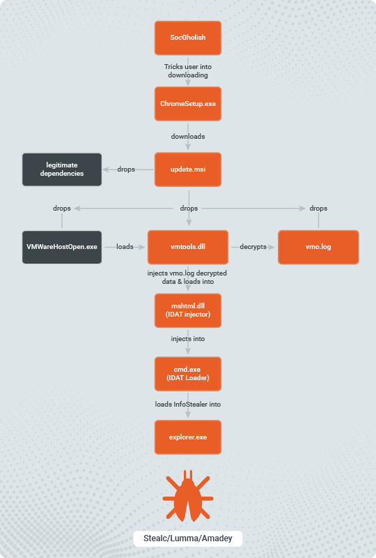


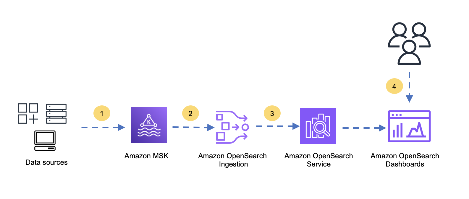

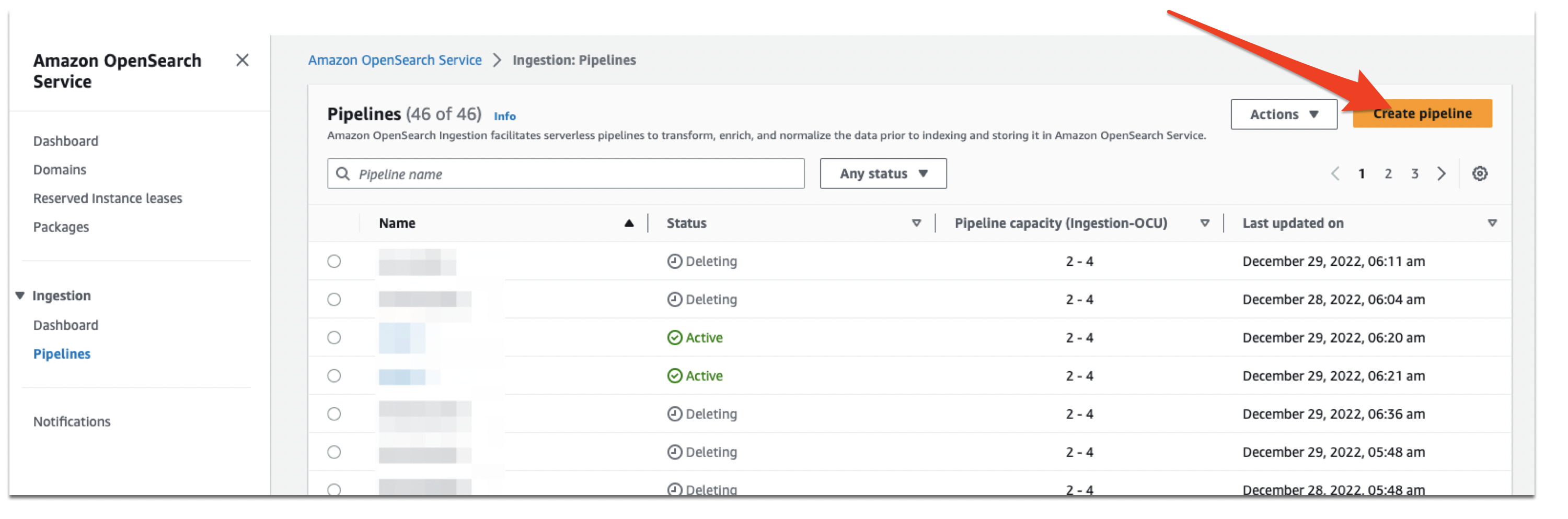
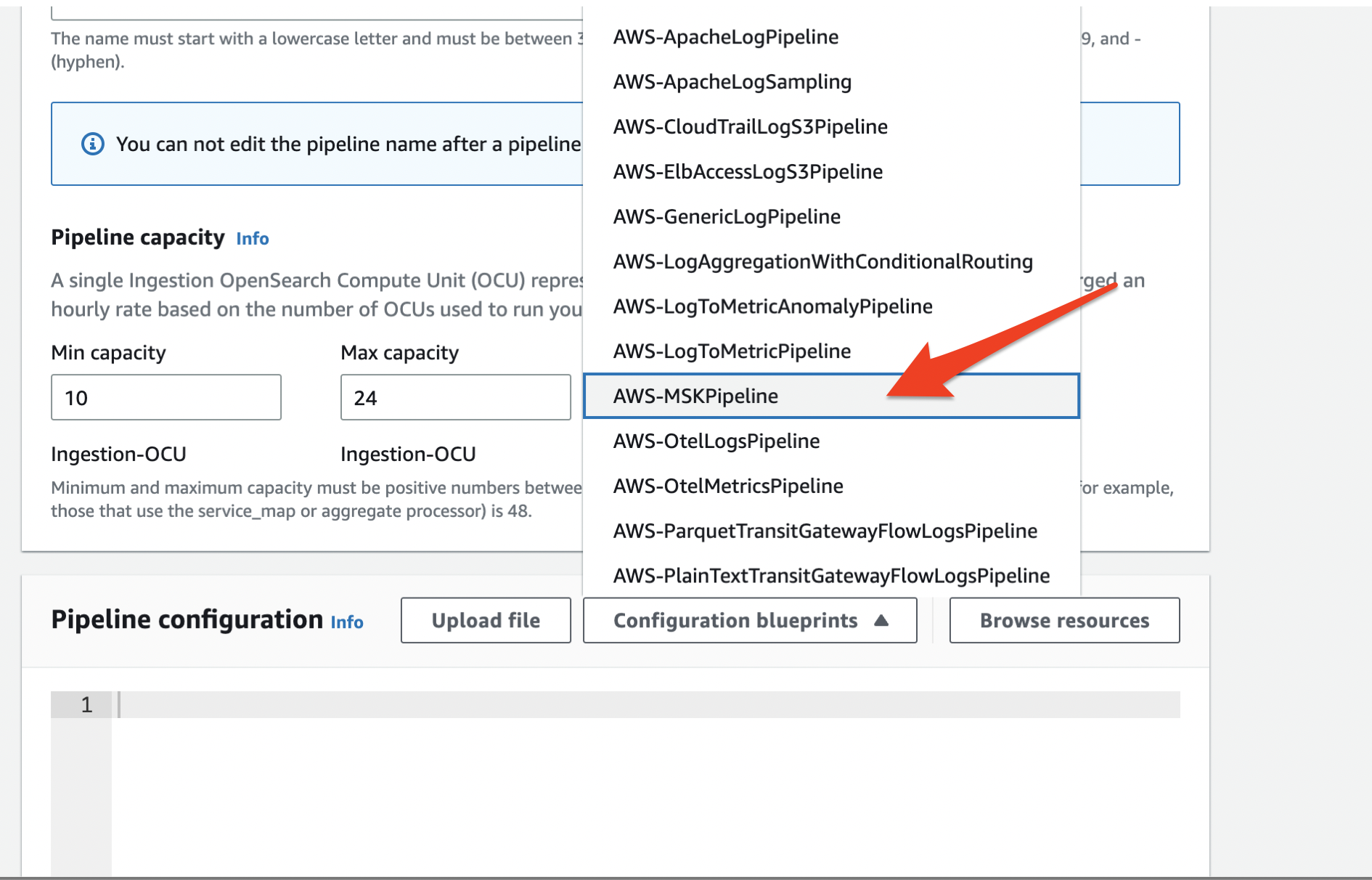
 Muthu Pitchaimani is a Search Specialist with Amazon OpenSearch Service. He builds large-scale search applications and solutions. Muthu is interested in the topics of networking and security, and is based out of Austin, Texas.
 Arjun Nambiar is a Product Manager with Amazon OpenSearch Service. He focusses on ingestion technologies that enable ingesting data from a wide variety of sources into Amazon OpenSearch Service at scale. Arjun is interested in large scale distributed systems and cloud-native technologies and is based out of Seattle, Washington.
 Raj Sharma is a Sr. SDM with Amazon OpenSearch Service. He builds large-scale distributed applications and solutions. Raj is interested in the topics of Analytics, databases, networking and security, and is based out of Palo Alto, California.
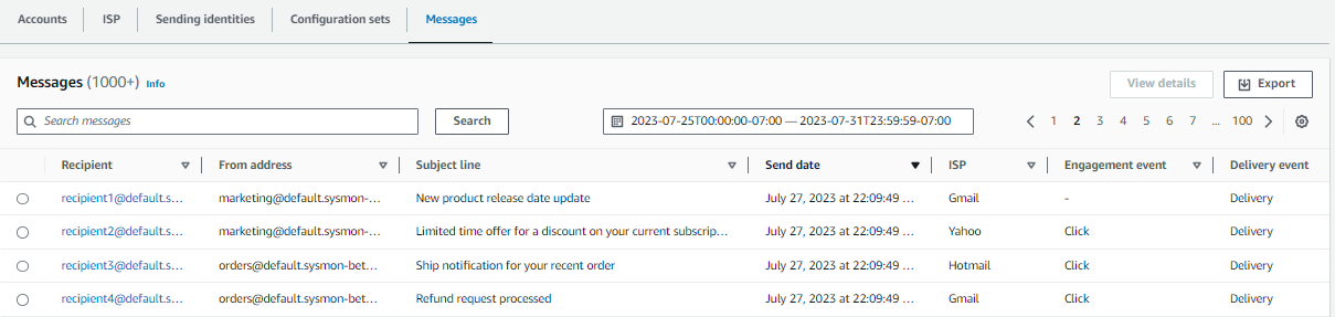

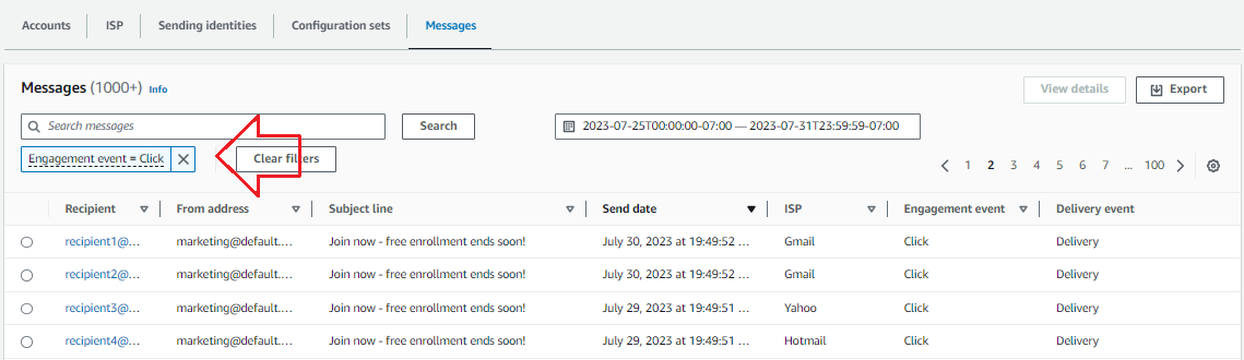
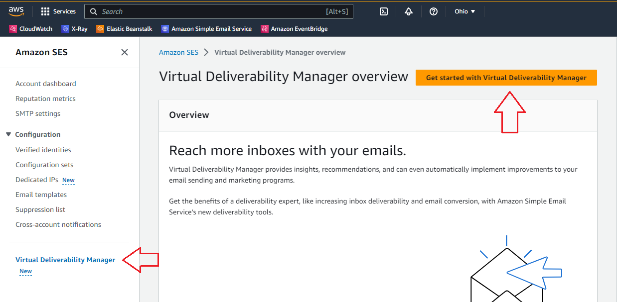

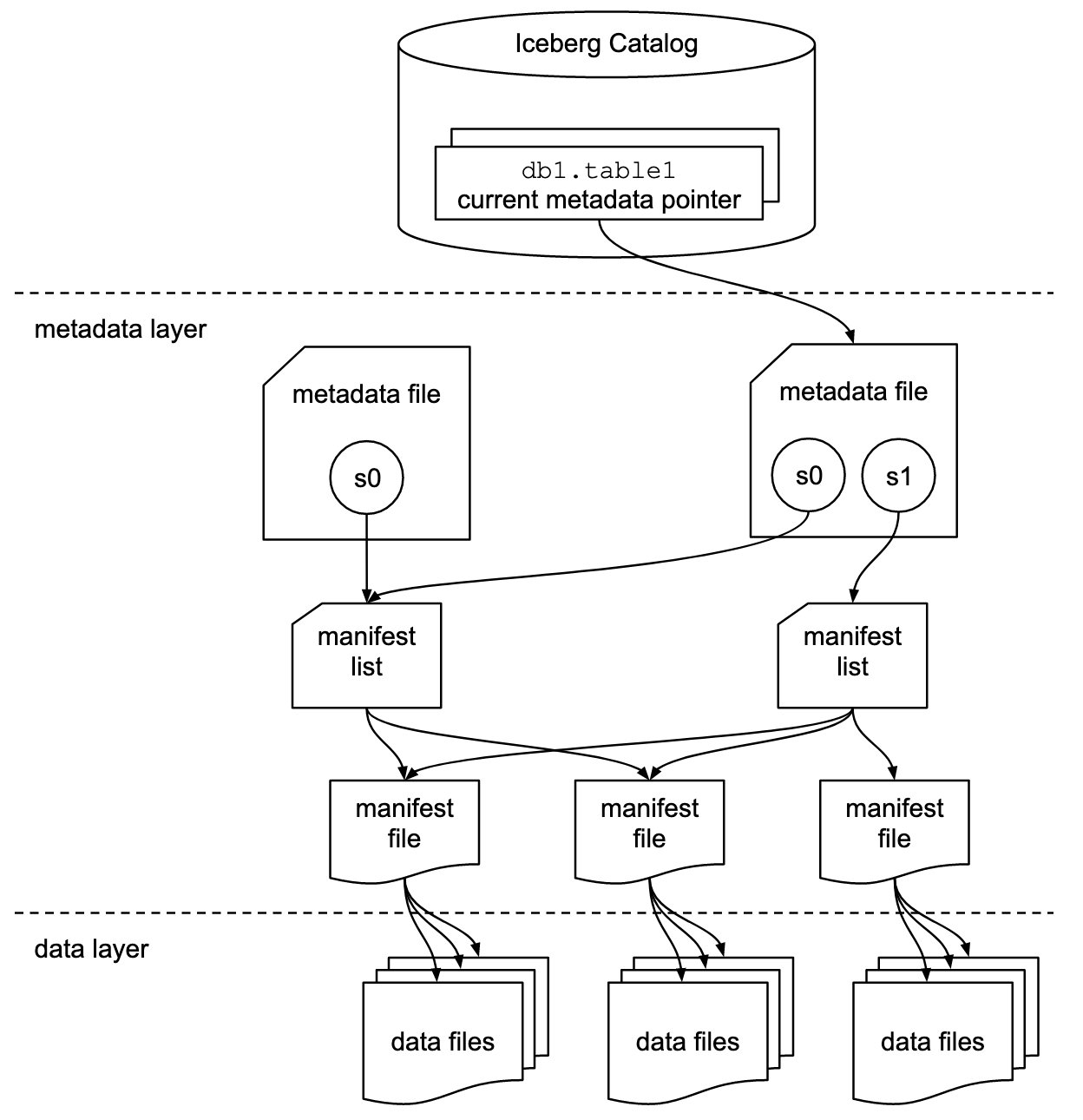


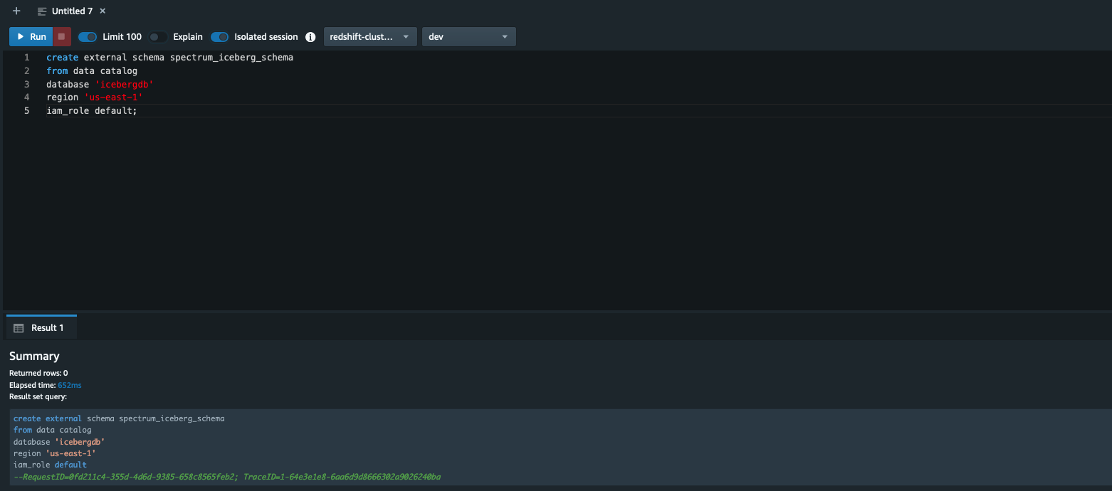
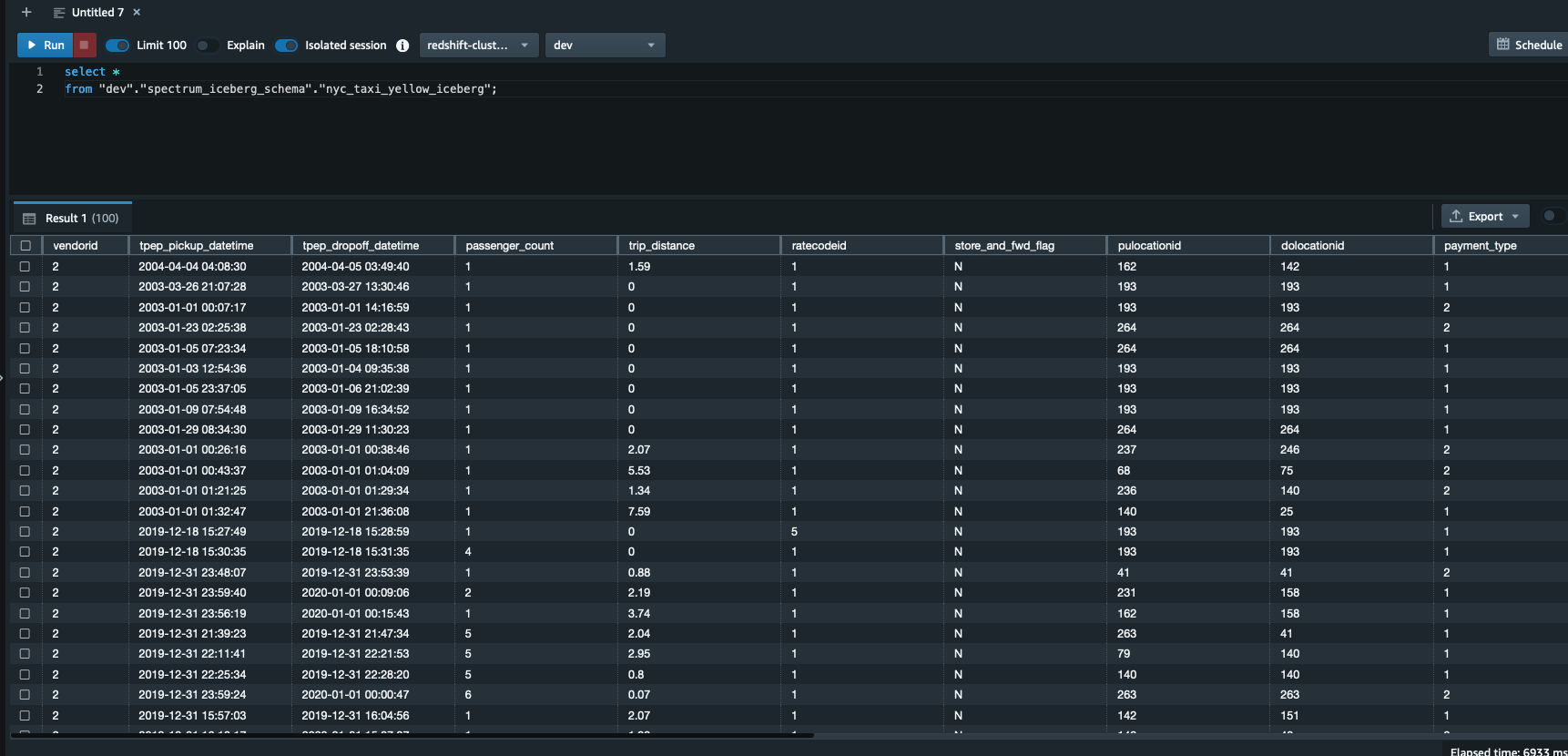

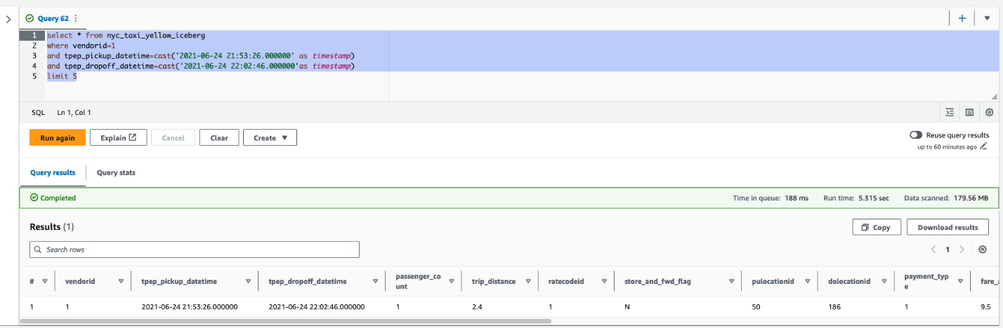
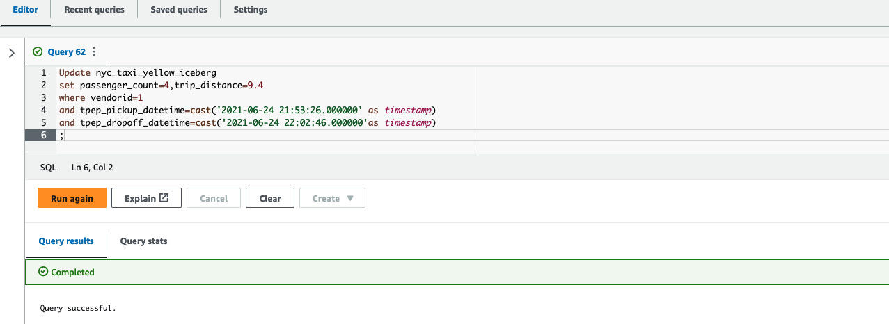


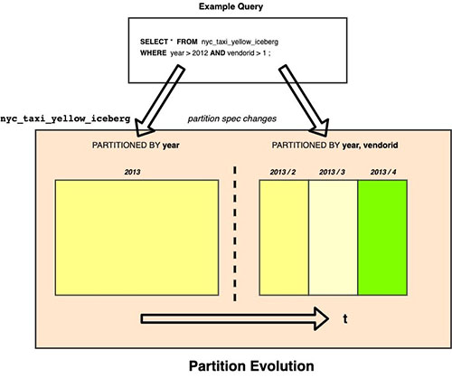

 Satish Sathiya is a Senior Product Engineer at Amazon Redshift. He is an avid big data enthusiast who collaborates with customers around the globe to achieve success and meet their data warehousing and data lake architecture needs.
 Joshua Luo is a Software Development Engineer for Amazon OpenSearch Serverless. He works on the systems that enable customers to manage and monitor their OpenSearch Serverless resources. He enjoys bouldering, photography, and videography in his free time.
 Satish Nandi is a Senior Technical Product Manager for Amazon OpenSearch Service.


 Ziad WALI is an Acceleration Lab Solutions Architect at Amazon Web Services. He has over 10 years of experience in databases and data warehousing where he enjoys building reliable, scalable and efficient solutions. Outside of work, he enjoys sports and spending time in nature.