The deal with DMCA 1201 reform

Post Syndicated from original https://blog.erratasec.com/2020/12/the-deal-with-dmca-1201-reform.html

There are two fights in Congress now against the DMCA, the “Digital Millennium Copyright Act”. One is over Section 512 covering “takedowns” on the web. The other is over Section 1201 covering “reverse engineering”, which weakens cybersecurity.

Even before digital computers, since the 1880s, an important principle of cybersecurity has been openness and transparency (“Kerckhoff’s Principle”). Only through making details public can security flaws be found, discussed, and fixed. This includes reverse-engineering to search for flaws.

Cybersecurity experts have long struggled against the ignorant who hold the naive belief we should instead coverup information, so that evildoers cannot find and exploit flaws. Surely, they believe, given just anybody access to critical details of our security weakens it. The ignorant have little faith in technology, that it can be made secure. They have more faith in government’s ability to control information.

Technologists believe this information coverup hinders well-meaning people and protects the incompetent from embarrassment. When you hide information about how something works, you prevent people on your own side from discovering and fixing flaws. It also means that you can’t hold those accountable for their security, since it’s impossible to notice security flaws until after they’ve been exploited. At the same time, the information coverup does not do much to stop evildoers. Technology can work, it can be perfected, but only if we can search for flaws.

It seems counterintuitive the revealing your encryption algorithms to your enemy is the best way to secure them, but history has proven time and again that this is indeed true. Encryption algorithms your enemy cannot see are insecure. The same is true of the rest of cybersecurity.

Today, I’m composing and posting this blogpost securely from a public WiFi hotspot because the technology is secure. It’s secure because of two decades of security researchers finding flaws in WiFi, publishing them, and getting them fixed.

Yet in the year 1998, ignorance prevailed with the “Digital Millennium Copyright Act”. Section 1201 makes reverse-engineering illegal. It attempts to secure copyright not through strong technological means, but by the heavy hand of government punishment.

The law was not completely ignorant. It includes an exception allow what it calls “security testing” — in theory. But that exception does not work in practice, imposing too many conditions on such research to be workable.

The U.S. Copyright Office has authority under the law to add its own exemptions every 3 years. It has repeatedly added exceptions for security research, but the process is unsatisfactory. It’s a protracted political battle every 3 years to get the exception back on the list, and each time it can change slightly. These exemptions are still less than what we want. This causes a chilling effect on permissible research. It would be better if such exceptions were put directly into the law.

You can understand the nature of the debate by looking at those on each side.

Those lobbying for the exceptions are those trying to make technology more secure, such as Rapid7, Bugcrowd, Duo Security, Luta Security, and Hackerone. These organizations have no interest in violating copyright — their only concern is cybersecurity, finding and fixing flaws.

The opposing side includes the copyright industry, as you’d expect, such as the “DVD” association who doesn’t want hackers breaking the DRM on DVDs.

However, much of the opposing side has nothing do with copyright as such.

This notably includes the three major voting machine suppliers in the United States: Dominion Voting, ES&S, and Hart InterCivic. Security professionals have been pointing out security flaws in their equipment for the past several years. These vendors are explicitly trying to coverup their security flaws by using the law to silence critics.

This goes back to the struggle mentioned at the top of this post. The ignorant and naive believe that we need to coverup information, so that hackers can’t discover flaws. This is expressed in their filing opposing the latest 3-year exemption:

The proponents are wrong and misguided in their argument that the Register’s allowing independent hackers unfettered access to election software is a necessary – or even appropriate – way to address the national security issues raised by election system security. The federal government already has ways of ensuring election system security through programs conducted by the EAC and DHS. These programs, in combination with testing done in partnership between system providers, independent voting system test labs and election officials, provide a high degree of confidence that election systems are secure and can be used to run fair and accurate elections. Giving anonymous hackers a license to attack critical infrastructure would not serve the public interest. 

Not only does this blatantly violate Kerckhoff’s Principle stated above, it was proven a fallacy in the last two DEF CON cybersecurity conferences. These conferences bought voting machines off eBay and presented them at the conference for anybody to hack. Widespread and typical vulnerabilities were found. These systems were certified as secure by state and federal governments, yet teenagers were able to trivially bypass the security of these systems.

The danger these companies are afraid of is not a nation state actor being able to play with these systems, but of teenagers playing with their systems at DEF CON embarrassing them by pointing out their laughable security. This proves Kerckhoff’s Principle.

That’s why the leading technology firms take the opposite approach to security than election systems vendors. This includes Apple, Amazon, Microsoft, Google, and so on. They’ve gotten over their embarrassment. They are every much as critical to modern infrastructure as election systems or the power grid. They publish their flaws roughly every month, along with a patch that fixes them. That’s why you end up having to patch your software every month. Far from trying to coverup flaws and punish researchers, they publicly praise researchers, and in many cases, offer “bug bounties” to encourage them to find more bugs.

It’s important to understand that the “security research” we are talking about is always “ad hoc” rather than formal.

These companies already do “formal” research and development. They invest billions of dollars in securing their technology. But no matter how much formal research they do, informal poking around by users, hobbyists, and hackers still finds unexpected things.

One reason is simply a corollary to the Infinite Monkey Theorem that states that an infinite number of monkeys banging on an infinite number of typewriters will eventually reproduce the exact works of William Shakespeare. A large number of monkeys banging on your product will eventually find security flaws.

A common example is a parent who brings their kid to work, who then plays around with a product doing things that no reasonable person would every conceive of, and accidentally breaks into the computer. Formal research and development focuses on the known threats, but has trouble of imagining unknown threats.

Another reason informal research is successful is how the modern technology stack works. Whether it’s a mobile phone, a WiFi enabled teddy bear for the kids, a connected pacemaker jolting the grandparent’s heart, or an industrial control computer controlling manufacturing equipment, all modern products share a common base of code.

Somebody can be an expert in an individual piece of code used in all these products without understanding anything about these products.

I experience this effect myself. I regularly scan the entire Internet looking for a particular flaw. All I see is the flaw itself, exposed to the Internet, but not anything else about the system I’ve probed. Maybe it’s a robot. Maybe it’s a car. Maybe it’s somebody’s television. Maybe it’s any one of the billions of IoT (“Internet of Things”) devices attached to the Internet. I’m clueless about the products — but an expert about the flaw.

A company, even as big as Apple or Microsoft, cannot hire enough people to be experts in every piece of technology they use. Instead, they can offer bounties encouraging those who are experts in obscure bits of technology to come forward and examine their products.

This ad hoc nature is important when looking at the solution to the problem. Many think this can be formalized, such as with the requirement of contacting a company asking for permission to look at their product before doing any reverse-engineering.

This doesn’t work. A security researcher will buy a bunch of used products off eBay to test out a theory. They don’t know enough about the products or the original vendor to know who they should contact for permission. This would take more effort to resolve than the research itself.

It’s solely informal and ad hoc “research” that needs protection. It’s the same as with everything else that preaches openness and transparency. Imagine if we had freedom of the press, but only for journalists who first were licensed by the government. Imagine if it were freedom of religion, but only for churches officially designated by the government.

Those companies selling voting systems they promise as being “secure” will never give permission. It’s only through ad hoc and informal security research, hostile to the interests of those companies, that the public interest will be advanced.

The current exemptions have a number of “gotchas” that seem reasonable, but which create an unacceptable chilling effect.

For example, they allow informal security research “as long as no other laws are violated”. That sounds reasonable, but with so many laws and regulations, it’s usually possible to argue they violated some obscure and meaningless law in their research. It means a security researcher is now threatened by years in jail for violating a regulation that would’ve resulted in a $10 fine during the course of their research.

Exceptions to the DMCA need to be clear and unambiguous that finding security bugs is not a crime. If the researcher commits some other crime during research, then prosecute them for that crime, not for violating the DMCA.

The strongest opposition to a “security research exemption” in the DMCA is going to come from the copyright industry itself — those companies who depend upon copyright for their existence, such as movies, television, music, books, and so on.

The United States position in the world is driven by intellectual property. Hollywood is not simply the center of American film industry, but the world’s film industry. Congress has an enormous incentive to protect these industries. Industry organizations like the RIAA and MPAA have enormous influence on Congress.

Many of us in tech believe copyright is already too strong. They’ve made a mockery of the Constitution’s statement of copyrights being for a “limited time”, which now means works copyrighted decades before you were born will still be under copyright decades after you die. Section 512 takedown notices are widely abused to silence speech.

Yet the copyright-protected industries perceive themselves as too weak. Once a copyrighted work is post to the Internet for anybody to download, it because virtually impossible to remove (like removing pee from a pool). Takedown notices only remove content from the major websites, like YouTube. They do nothing to remove content from the “dark web”.

Thus, they jealously defend against any attempt that would weaken their position. This includes “security research exemptions”, which threatens “DRM” technologies that prevent copying.

One fear is of security researchers themselves, that in the process of doing legitimate research that they’ll find and disclose other secrets, such as the encryption keys that protect DVDs from being copied, that are built into every DVD player on the market. There is some truth to that, as security researchers have indeed publish some information that the industries didn’t want published, such as the DVD encryption algorithm.

The bigger fear is that evildoers trying to break DRM will be free to do so, claiming their activities are just “security research”. They would be free to openly collaborate with each other, because it’s simply research, while privately pirating content.

But these fears are overblown. Commercial piracy is already forbidden by other laws, and underground piracy happens regardless of the law.

This law has little impact on whether reverse-engineering happens so much as impact whether the fruits of research are published. And that’s the key point: we call it “security research”, but all that’s meaningful is “published security research”.

In other words, we are talking about a minor cost to copyright compared with a huge cost to cybersecurity. The cybersecurity of voting machines is a prime example: voting security is bad, and it’s not going to improve until we can publicly challenge it. But we can’t easily challenge voting security without being prosecuted under the DMCA.

Conclusion

The only credible encryption algorithms are public ones. The only cybersecurity we trust is cybersecurity that we can probe and test, where most details are publicly available. That such transparency is necessary to security has been recognized since the 1880s with Kerckhoff’s Principle. Yet, the naive still believe in coverups. As the election industry claimed in their brief: “Giving anonymous hackers a license to attack critical infrastructure would not serve the public interest”. Giving anonymous hackers ad hoc, informal access to probe critical infrastructure like voting machines not only serves the public interest, but is necessary to the public interest. As has already been proven, voting machines have cybersecurity weaknesses that they are covering up, which can only be revealed by anonymous hackers.

This research needs to be ad hoc and informal. Attempts at reforming the DMCA, or the Copyright Office’s attempt at exemptions, get modified into adding exemptions for formal research. This ends up having the same chilling effect on research while claiming to allow research.

Copyright, like other forms of intellectual property, is important, and it’s proper for government to protect it. Even radical anarchists in our industry want government to protect “copyleft”, the use of copyright to keep open-source code open.

But it’s not so important that it should allow abuse to silence security research. Transparency and ad hoc testing is critical to research, and is more and more often being silenced using copyright law.

Harness the power of your data with AWS Analytics

Post Syndicated from Rahul Pathak original https://aws.amazon.com/blogs/big-data/harness-the-power-of-your-data-with-aws-analytics/

2020 has reminded us of the need to be agile in the face of constant and sudden change. Every customer I’ve spoken to this year has had to do things differently because of the pandemic. Some are focusing on driving greater efficiency in their operations and others are experiencing a massive amount of growth. Across the board, I see organizations looking to use their data to make better decisions quickly as changes occur. Such agility requires that they integrate terabytes to petabytes and sometimes exabytes of data that were previously siloed in order to get a complete view of their customers and business operations. Traditional on-premises data analytics solutions can’t handle this approach because they don’t scale well enough and are too expensive. As a result, we’re seeing an acceleration in customers looking to modernize their data and analytics infrastructure by moving to the cloud.

Customer data in the real world

To analyze these vast amounts of data, many companies are moving all their data from various silos into a single location, often called a data lake, to perform analytics and machine learning (ML). These same companies also store data in purpose-built data stores for the performance, scale, and cost advantages they provide for specific use cases. Examples of such data stores include data warehouses—to get quick results for complex queries on structured data—and technologies like Elasticsearch—to quickly search and analyze log data to monitor the health of production systems. A one-size-fits-all approach to data analytics no longer works because it inevitably leads to compromises.

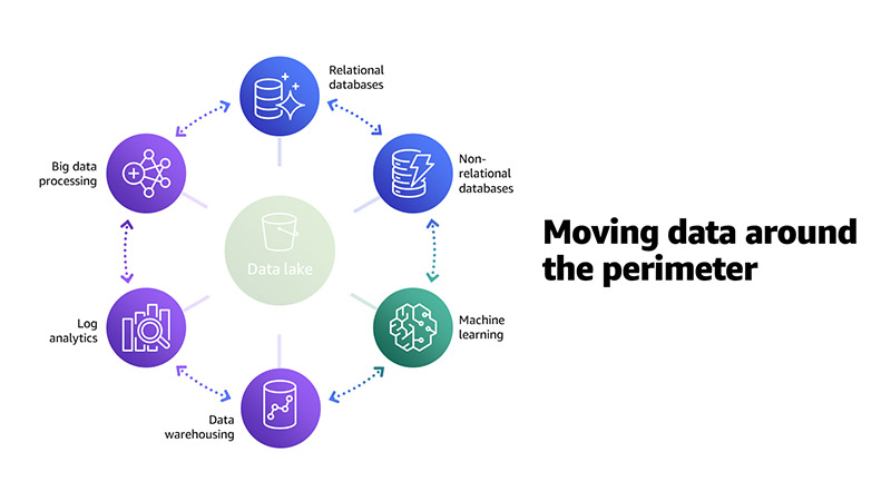
To get the most from their data lakes and these purpose-built stores, customers need to move data between these systems easily. For instance, clickstream data from web applications can be collected directly in a data lake and a portion of that data can be moved out to a data warehouse for daily reporting. We think of this concept as inside-out data movement.

Similarly, customers also move data in the other direction:  from the outside-in. For example, they copy query results for sales of products in a given region from their data warehouse into their data lake to run product recommendation algorithms against a larger data set using ML.

Finally, in other situations, customers want to move data from one purpose-built data store to another: around-the-perimeter. For example, they may copy the product catalog data stored in their database to their search service in order to make it easier to look through their product catalog and offload the search queries from the database.

As data in these data lakes and purpose-built stores continues to grow, it becomes harder to move all this data around. We call this data gravity.

To make decisions with speed and agility, customers need to be able to use a central data lake and a ring of purpose-built data services around that data lake. They also need to acknowledge data gravity by easily moving the data they need between these data stores in a secure and governed way.

To meet these needs, customers require a data architecture that supports the following:

  • Building a scalable data lake rapidly.
  • Using a broad and deep collection of purpose-built data services that provide the performance required for use-cases like interactive dashboards and log analytics.
  • Moving data seamlessly between the data lake and purpose-built data services and between those purpose-built data services.
  • Ensuring compliance via a unified way to secure, monitor, and manage access to data.
  • Scaling systems at low cost without compromising on performance.

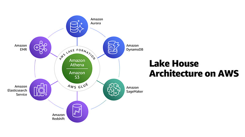
We call this modern approach to analytics the Lake House Architecture.

Lake House Architecture on AWS

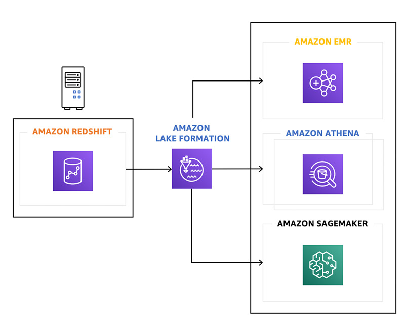
A Lake House Architecture acknowledges the idea that taking a one-size-fits-all approach to analytics eventually leads to compromises. It is not simply about integrating a data lake with a data warehouse, but rather about integrating a data lake, a data warehouse, and purpose-built stores and enabling unified governance and easy data movement. The diagram below shows the Lake House Architecture on AWS.

Let’s take a look at how the Lake House Architecture on AWS and some of the new capabilities we announced at re:Invent 2020 help our customers meet each of the requirements above..

Scalable data lakes

Amazon Simple Storage Service (Amazon S3) is the best place to build a data lake because it has unmatched durability, availability, and scalability; the best security, compliance, and audit capabilities; the fastest performance at the lowest cost; the most ways to bring data in; and the most partner integrations.

However, setting up and managing data lakes involves a lot of manual and time-consuming tasks such as loading data from diverse sources, monitoring data flows, setting up partitions, turning on encryption and managing keys, reorganizing data into columnar format, and granting and auditing access. To help make this easier, we built AWS Lake Formation. Lake Formation helps our customers build secure data lakes in the cloud in days instead of months. Lake Formation collects and catalogs data from databases and object storage, moves the data into an Amazon S3 data lake, cleans and classifies data using ML algorithms, and secures access to sensitive data.

In addition, we just announced three new capabilities for AWS Lake Formation in preview:  ACID transactions and governed tables for concurrent updates and consistent query results and query acceleration through automatic file compaction. The preview introduces new APIs that support atomic, consistent, isolated, and durable (ACID) transactions using a new data lake table type, called a governed table. Governed tables allow multiple users to concurrently insert, delete, and modify rows across tables, while still allowing other users to simultaneously run analytical queries and ML models on the same data sets. Automatic file compaction combines small files into larger files to make queries by up to seven times faster.

Purpose-built analytics services

AWS offers the broadest and deepest portfolio of purpose-built analytics services, including Amazon Athena, Amazon EMR, Amazon Elasticsearch Service, Amazon Kinesis, and Amazon Redshift. These services are all built to be best-of-breed, which means you never have to compromise on performance, scale, or cost when using them. For example, Amazon Redshift delivers up to three times better price performance than other cloud data warehouses, and Apache Spark on EMR runs 1.7 times faster than standard Apache Spark 3.0, which means petabyte-scale analysis can be run at less than half of the cost of traditional on-premises solutions.

We’re always innovating to meet our customer’s needs with new capabilities and features in these purpose-built services. For example, to help with additional cost savings and deployment flexibility, today we announced the general availability of Amazon EMR on Amazon Elastic Kubernetes Service (EKS). This offers a new deployment option of fully managed Amazon EMR on Amazon EKS. Until now, customers had to choose between running managed Amazon EMR on EC2 and self-managing their own Apache Spark on Amazon EKS. Now, analytical workloads can be consolidated with microservices and other Kubernetes-based applications on the same Amazon EKS cluster, enabling improved resource utilization, simpler infrastructure management, and the ability to use a single set of tools for monitoring.

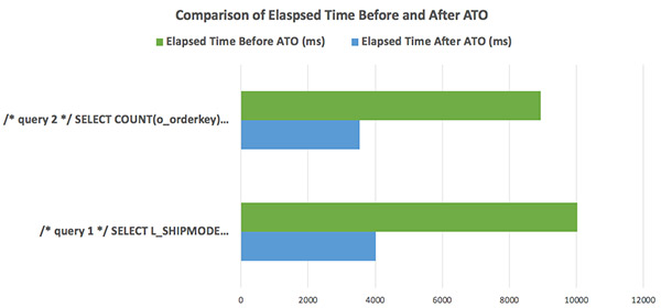
For faster data warehousing performance, we announced the general availability of Automatic Table Optimizations (ATO) for Amazon Redshift. ATO simplifies performance tuning of Amazon Redshift data warehouses by using ML to automate optimization tasks such as setting distribution and sort keys to give you the best possible performance without the overhead of manual performance tuning.

We also announced the preview of Amazon QuickSight Q to make it even easier and faster for your business users to get insights from your data. QuickSight Q uses ML to generate a data model that automatically understands the meaning and relationships of business data. It enables users to ask ad hoc questions about their business data in human-readable language and get accurate answers in seconds. As a result, business users can now get answers to their questions instantly without having to wait for modeling by thinly-staffed business intelligence (BI) teams.

Seamless data movement

With data stored in a number of different systems, customers need to be able to easily move that data between all of their services and data stores:  inside-out, outside-in, and around-the-perimeter. No other analytics provider makes it as easy to move data at scale to where it’s needed most. AWS Glue is a serverless data integration service that allows you to easily prepare data for analytics, machine learning, and application development. AWS Glue provides all the capabilities needed for data integration, so insights can be gained in minutes instead of months. Amazon Redshift and Athena both support federated queries, the ability to run queries across data stored in operational databases, data warehouses, and data lakes to provide insights across multiple data sources with no data movement and no need to set up and maintain complex extract, transform, and load (ETL) pipelines.

To make it even easier to combine and replicate data across multiple data stores, last week we announced the preview of AWS Glue Elastic Views. AWS Glue Elastic Views lets developers create materialized views across a wide variety of databases and data stores using familiar SQL, reducing the time it takes to combine and replicate data across data stores from months to minutes. AWS Glue Elastic Views handles copying and combining data from source to target data stores, continuously monitors for changes in source data stores, and updates the materialized views automatically to ensure data accessed is always up-to-date.

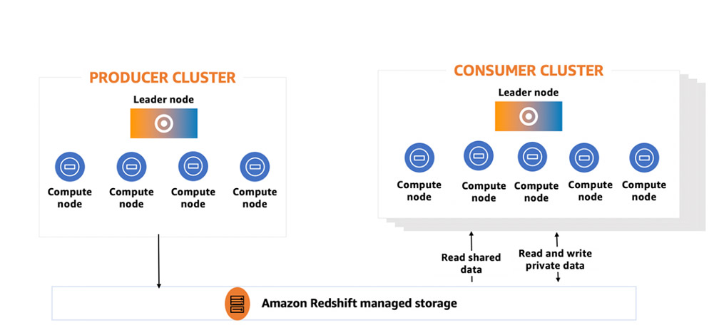
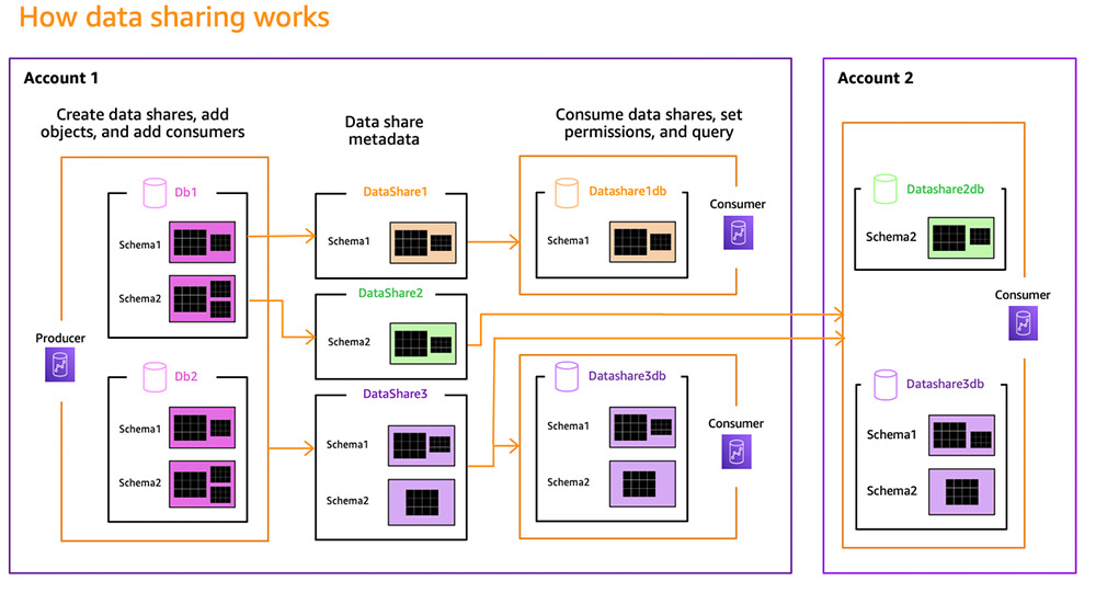
We also announced the preview of Amazon Redshift data sharing. Data sharing provides a secure and easy way to share live data across multiple Amazon Redshift clusters inside the organization and externally without the need to make copies or the complexity of moving around data. Customers can use data sharing to run analytics workloads that use the same data in separate compute clusters in order to meet the performance requirements of each workload and track usage by each business group. For example, customers can set up a central ETL cluster and share data with multiple BI clusters to provide workload isolation and chargeback.

Unified governance

One of the most important pieces of a modern analytics architecture is the ability to authorize, manage, and audit access to data. Enabling such a capability can be challenging because managing security, access control, and audit trails across all the data stores in an organization is complex and time-consuming. It’s also error-prone because it requires manually maintaining access control lists and audit policies across all storage systems, each with different security, data access, and audit mechanisms.

With capabilities like centralized access control and policies combined with column and row-level filtering, AWS gives customers the fine-grained access control and governance to manage access to data across a data lake and purpose-built data stores from a single point of control.

Today, we also announced the preview of row-level security for AWS Lake Formation, which makes it even easier to control access for all the people and applications that need to share data. Row-level security allows for filtering and setting data access policies at the row level. For example, you can now set a policy that gives a regional sales manager access to only the sales data for their region. This level of filtering eliminates the need to maintain different copies of data lake tables for different user groups, saving you operational overhead and unnecessary storage costs.

Performance and cost-effectiveness

At AWS, we’re committed to providing the best performance at the lowest cost across all analytics services and we continue to innovate to improve the price-performance of our services. In addition to industry-leading price performance for services like Amazon Redshift and Amazon EMR, Amazon S3 intelligent tiering saves customers up to 40% on storage costs for data stored in a data lake, and Amazon EC2 provides access to over 350 instance types, up to 400Gbps ethernet networking, and the ability to choose between On-Demand, Reserved, and Spot instances. We announced Amazon EMR support for Amazon EC2 M6g instances powered by AWS Graviton2 processors in October, providing up to 35% lower cost and up to 15% improved performance. Our customers can also take advantage of AWS Savings Plans, a flexible pricing model that provides savings of up to 72% on AWS compute usage.

To set the foundation for the new scale of data, we also shared last week that the AQUA (Advanced Query Accelerator) for Amazon Redshift preview is now open to all customers and will be generally available in January 2021. AQUA is a new distributed and hardware-accelerated cache that brings compute to the storage layer, and delivers up to ten times faster query performance than other cloud data warehouses. AQUA is available on Amazon Redshift RA3 instances at no additional cost, and customers can take advantage of the AQUA performance improvements without any code changes.

Learn More and Get Started Today

Whatever a customer is looking to do with data, AWS Analytics can offer a solution. We provide the broadest and deepest portfolio of purpose-built analytics services to realize a Lake House Architecture. Our portfolio includes the most scalable data lakes, purpose-built analytics services, seamless data movement, and unified governance – all delivered with the best performance at the lowest cost.

Read all the Analytics announcements from AWS re:Invent 2020 at What’s New at AWS re:Invent? and apply for the analytics previews using the links below. Also dive deeper by watching the more than 40 analytics sessions that were part of AWS re:Invent 2020. Simply visit the session catalog and choose the Analytics track to review past sessions and add upcoming ones to your calendar.

Finally, take advantage of the AWS Data Lab. The AWS Data Lab offers opportunities for customers and AWS technical resources to engage and accelerate data and analytics modernization initiatives.

Announcement and Preview Links


About the Author

Rahul Pathak is Vice President of Analytics at AWS and is responsible for Amazon Athena, Amazon Elasticsearch Service, EMR, Glue, Lake Formation, and Redshift. Over his nine years at AWS, he has focused on managed database, analytics, and database services. Rahul has over twenty years of experience in technology and has co-founded two companies, one focused on digital media analytics and the other on IP-geolocation. He holds a degree in Computer Science from MIT and an Executive MBA from the University of Washington.


Get started with fine-grained access control in Amazon Elasticsearch Service

Post Syndicated from Jon Handler original https://aws.amazon.com/blogs/security/get-started-with-fine-grained-access-control-in-amazon-elasticsearch-service/

Amazon Elasticsearch Service (Amazon ES) provides fine-grained access control, powered by the Open Distro for Elasticsearch security plugin. The security plugin adds Kibana authentication and access control at the cluster, index, document, and field levels that can help you secure your data. You now have many different ways to configure your Amazon ES domain to provide access control. In this post, I offer basic configuration information to get you started.

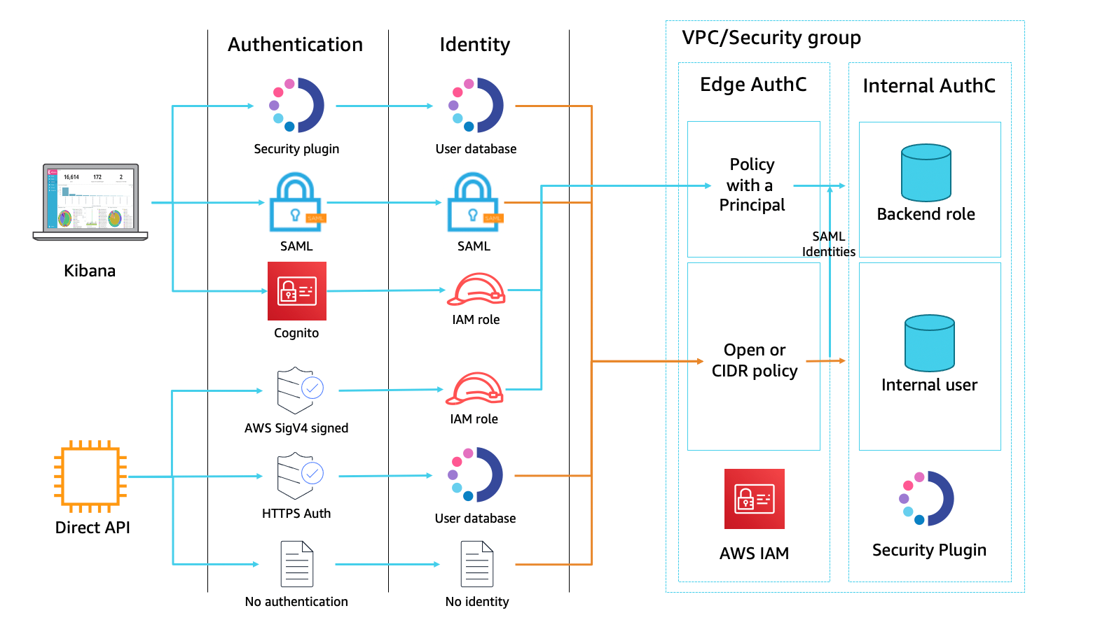
Figure 1: A high-level view of data flow and security

Figure 1: A high-level view of data flow and security

Figure 1 details the authentication and access control provided in Amazon ES. The left half of the diagram details the different methods of authenticating. Looking horizontally, requests originate either from Kibana or directly access the REST API. When using Kibana, you can use a login screen powered by the Open Distro security plugin, your SAML identity provider, or Amazon Cognito. Each of these methods results in an authenticated identity: SAML providers via the response, Amazon Cognito via an AWS Identity and Access Management (IAM) identity, and Open Distro via an internal user identity. When you use the REST API, you can use AWS Signature V4 request signing (SigV4 signing), or user name and password authentication. You can also send unauthenticated traffic, but your domain should be configured to reject all such traffic.

The right side of the diagram details the access control points. You can consider the handling of access control in two phases to better understand it—authentication at the edge by IAM and authentication in the Amazon ES domain by the Open Distro security plugin.

First, requests from Kibana or direct API calls have to reach your domain endpoint. If you follow best practices and the domain is in an Amazon Virtual Private Cloud (VPC), you can use Amazon Elastic Compute Cloud (Amazon EC2) security groups to allow or deny traffic based on the originating IP address or security group of the Amazon EC2 instances. Best practice includes least privilege based on subnet ACLs and security group ingress and egress restrictions. In this post, we assume that your requests are legitimate, meet your access control criteria, and can reach your domain.

When a request reaches the domain endpoint—the edge of your domain—, it can be anonymous or it can carry identity and authentication information as described previously. Each Amazon ES domain carries a resource-based IAM policy. With this policy, you can allow or deny traffic based on an IAM identity attached to the request. When your policy specifies an IAM principal, Amazon ES evaluates the request against the allowed Actions in the policy and allows or denies the request. If you don’t have an IAM identity attached to the request (SAML assertion, or user name and password) you should leave the domain policy open and pass traffic through to fine-grained access control in Amazon ES without any checks. You should employ IAM security best practices and add additional IAM restrictions for direct-to-API access control once your domain is set up.

The Open Distro for Elasticsearch security plugin has its own internal user database for user name and password authentication and handles access control for all users. When traffic reaches the Elasticsearch cluster, the plugin validates any user name and password authentication information against this internal database to identify the user and grant a set of permissions. If a request comes with identity information from either SAML or an IAM role, you map that backend role onto the roles or users that you have created in Open Distro security.

Amazon ES documentation and the Open Distro for Elasticsearch documentation give more information on all of these points. For this post, I walk through a basic console setup for a new domain.

Console set up

The Amazon ES console provides a guided wizard that lets you configure—and reconfigure—your Amazon ES domain. Step 1 offers you the opportunity to select some predefined configurations that carry through the wizard. In step 2, you choose the instances to deploy in your domain. In Step 3, you configure the security. This post focuses on step 3. See also these tutorials that explain using an IAM master user and using an HTTP-authenticated master user.

Note: At the time of writing, you cannot enable fine-grained access control on existing domains; you must create a new domain and enable the feature at domain creation time. You can use fine-grained access control with Elasticsearch versions 6.8 and later.

Set your endpoint

Amazon ES gives you a DNS name that resolves to an IP address that you use to send traffic to the Elasticsearch cluster in the domain. The IP address can be in the IP space of the public internet, or it can resolve to an IP address in your VPC. While—with fine-grained access control—you have the means of securing your cluster even when the endpoint is a public IP address, we recommend using VPC access as the more secure option. Shown in Figure 2.

Figure 2: Select VPC access

Figure 2: Select VPC access

With the endpoint in your VPC, you use security groups to control which ports accept traffic and limit access to the endpoints of your Amazon ES domain to IP addresses in your VPC. Make sure to use least privilege when setting up security group access.

Enable fine-grained access control

You should enable fine-grained access control. Shown in Figure 3.

Figure 3: Enabled fine-grained access control

Figure 3: Enabled fine-grained access control

Set up the master user

The master user is the administrator identity for your Amazon ES domain. This user can set up additional users in the Amazon ES security plugin, assign roles to them, and assign permissions for those roles. You can choose user name and password authentication for the master user, or use an IAM identity. User name and password authentication, shown in Figure 4, is simpler to set up and—with a strong password—may provide sufficient security depending on your use case. We recommend you follow your organization’s policy for password length and complexity. If you lose this password, you can return to the domain’s dashboard in the AWS Management Console and reset it. You’ll use these credentials to log in to Kibana. Following best practices on choosing your master user, you should move to an IAM master user once setup is complete.

Note: Password strength is a function of length, complexity of characters (e.g., upper and lower case letters, numbers, and special characters), and unpredictability to decrease the likelihood the password could be guessed or cracked over a period of time.


Figure 4: Setting up the master username and password

Figure 4: Setting up the master username and password

Do not enable Amazon Cognito authentication

When you use Kibana, Amazon ES includes a login experience. You currently have three choices for the source of the login screen:

  1. The Open Distro security plugin
  2. Amazon Cognito
  3. Your SAML-compliant system

You can apply fine-grained access control regardless of how you log in. However, setting up fine-grained access control for the master user and additional users is most straightforward if you use the login experience provided by the Open Distro security plugin. After your first login, and when you have set up additional users, you should migrate to either Cognito or SAML for login, taking advantage of the additional security they offer. To use the Open Distro login experience, disable Amazon Cognito authentication, as shown in Figure 5.

Figure 5: Amazon Cognito authentication is not enabled

Figure 5: Amazon Cognito authentication is not enabled

If you plan to integrate with your SAML identity provider, check the Prepare SAML authentication box. You will complete the set up when the domain is active.

Figure 6: Choose Prepare SAML authentication if you plan to use it

Figure 6: Choose Prepare SAML authentication if you plan to use it

Use an open access policy

When you create your domain, you attach an IAM policy to it that controls whether your traffic must be signed with AWS SigV4 request signing for authentication. Policies that specify an IAM principal require that you use AWS SigV4 signing to authenticate those requests. The domain sends your traffic to IAM, which authenticates signed requests to resolve the user or role that sent the traffic. The domain and IAM apply the policy access controls and either accept the traffic or reject it based on the commands. This is done down to the index level for single-index API calls.

When you use fine-grained access control, your traffic is also authenticated by the Amazon ES security plugin, which makes the IAM authentication redundant. Create an open access policy, as shown in Figure 7, which doesn’t specify a principal and so doesn’t require request signing. This may be acceptable, since you can choose to require an authenticated identity on all traffic. The security plugin authenticates the traffic as above, providing access control based on the internal database.

Figure 7: Selected open access policy

Figure 7: Selected open access policy

Encrypted data

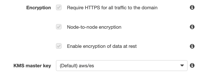
Amazon ES provides an option to encrypt data in transit and at rest for any domain. When you enable fine-grained access control, you must use encryption with the corresponding checkboxes automatically checked and not changeable. These include Transport Layer Security (TLS) for requests to the domain and for traffic between nodes in the domain, and encryption of data at rest through AWS Key Management Service (KMS). Shown in Figure 8.

Figure 8: Enabled encryption

Figure 8: Enabled encryption

Accessing Kibana

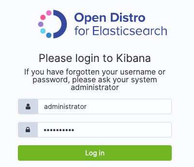
When you complete the domain creation wizard, it takes about 10 minutes for your domain to activate. Return to the console and the Overview tab of your Amazon ES dashboard. When the Domain Status is Active, select the Kibana URL. Since you created your domain in your VPC, you must be able to access the Kibana endpoint via proxy, VPN, SSH tunnel, or similar. Use the master user name and password that you configured earlier to log in to Kibana, as shown in Figure 9. As detailed above, you should only ever log in as the master user to set up additional users—administrators, users with read-only access, and others.

Figure 9: Kibana login page

Figure 9: Kibana login page

Conclusion

Congratulations, you now know the basic steps to set up the minimum configuration to access your Amazon ES domain with a master user. You can examine the settings for fine-grained access control in the Kibana console Security tab. Here, you can add additional users, assign permissions, map IAM users to security roles, and set up your Kibana tenancy. We’ll cover those topics in future posts.

If you have feedback about this post, submit comments in the Comments section below. If you have questions about this post, start a new thread on the Amazon Elasticsearch Service forum or contact AWS Support.

Want more AWS Security how-to content, news, and feature announcements? Follow us on Twitter.

Author

Jon Handler

Jon is a Principal Solutions Architect at AWS. He works closely with the CloudSearch and Elasticsearch teams, providing help and guidance to a broad range of customers who have search workloads that they want to move to the AWS Cloud. Prior to joining AWS, Jon’s career as a software developer included four years of coding a large-scale, eCommerce search engine. Jon holds a Bachelor of the Arts from the University of Pennsylvania, and a Master of Science and a Ph. D. in Computer Science and Artificial Intelligence from Northwestern University.

Author

Sajeev Attiyil Bhaskaran

Sajeev is a Senior Cloud Engineer focused on big data and analytics. He works with AWS customers to provide architectural and engineering assistance and guidance. He dives deep into big data technologies and streaming solutions. He also does onsite and online sessions for customers to design best solutions for their use cases. In his free time, he enjoys spending time with his wife and daughter.

Field Notes: Ingest and Visualize Your Flat-file IoT Data with AWS IoT Services

Post Syndicated from Paul Ramsey original https://aws.amazon.com/blogs/architecture/field-notes-ingest-and-visualize-your-flat-file-iot-data-with-aws-iot-services/

Customers who maintain manufacturing facilities often find it challenging to ingest, centralize, and visualize IoT data that is emitted in flat-file format from their factory equipment. While modern IoT-enabled industrial devices can communicate over standard protocols like MQTT, there are still some legacy devices that generate useful data but are only capable of writing it locally to a flat file. This results in siloed data that is either analyzed in a vacuum without the broader context, or it is not available to business users to be analyzed at all.

AWS provides a suite of IoT and Edge services that can be used to solve this problem. In this blog, I walk you through one method of leveraging these services to ingest hard-to-reach data into the AWS cloud and extract business value from it.

Overview of solution

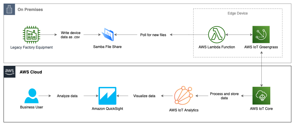
This solution provides a working example of an edge device running AWS IoT Greengrass with an AWS Lambda function that watches a Samba file share for new .csv files (presumably containing device or assembly line data). When it finds a new file, it will transform it to JSON format and write it to AWS IoT Core. The data is then sent to AWS IoT Analytics for processing and storage, and Amazon QuickSight is used to visualize and gain insights from the data.

Samba file share solution diagram

Since we don’t have an actual on-premises environment to use for this walkthrough, we’ll simulate pieces of it:

  • In place of the legacy factory equipment, an EC2 instance running Windows Server 2019 will generate data in .csv format and write it to the Samba file share.
    • We’re using a Windows Server for this function to demonstrate that the solution is platform-agnostic. As long as the flat file is written to a file share, AWS IoT Greengrass can ingest it.
  • An EC2 instance running Amazon Linux will act as the edge device and will host AWS IoT Greengrass Core and the Samba share.
    • In the real world, these could be two separate devices, and the device running AWS IoT Greengrass could be as small as a Raspberry Pi.

Prerequisites

For this walkthrough, you should have the following prerequisites:

  • An AWS Account
  • Access to provision and delete AWS resources
  • Basic knowledge of Windows and Linux server administration
  • If you’re unfamiliar with AWS IoT Greengrass concepts like Subscriptions and Cores, review the AWS IoT Greengrass documentation for a detailed description.

Walkthrough

First, we’ll show you the steps to launch the AWS IoT Greengrass resources using AWS CloudFormation. The AWS CloudFormation template is derived from the template provided in this blog post. Review the post for a detailed description of the template and its various options.

  1. Create a key pair. This will be used to access the EC2 instances created by the CloudFormation template in the next step.
  2. Launch a new AWS CloudFormation stack in the N. Virginia (us-east-1) Region using iot-cfn.yml, which represents the simulated environment described in the preceding bullet.
    •  Parameters:
      • Name the stack IoTGreengrass.
      • For EC2KeyPairName, select the EC2 key pair you just created from the drop-down menu.
      • For SecurityAccessCIDR, use your public IP with a /32 CIDR (i.e. 1.1.1.1/32).
      • You can also accept the default of 0.0.0.0/0 if you can have SSH and RDP open to all sources on the EC2 instances in this demo environment.
      • Accept the defaults for the remaining parameters.
  •  View the Resources tab after stack creation completes. The stack creates the following resources:
    • A VPC with two subnets, two route tables with routes, an internet gateway, and a security group.
    • Two EC2 instances, one running Amazon Linux and the other running Windows Server 2019.
    • An IAM role, policy, and instance profile for the Amazon Linux instance.
    • A Lambda function called GGSampleFunction, which we’ll update with code to parse our flat-files with AWS IoT Greengrass in a later step.
    • An AWS IoT Greengrass Group, Subscription, and Core.
    • Other supporting objects and custom resource types.
  • View the Outputs tab and copy the IPs somewhere easy to retrieve. You’ll need them for multiple provisioning steps below.

3. Review the AWS IoT Greengrass resources created on your behalf by CloudFormation:

    • Search for IoT Greengrass in the Services drop-down menu and select it.
    • Click Manage your Groups.
    • Click file_ingestion.
    • Navigate through the SubscriptionsCores, and other tabs to review the configurations.

Leveraging a device running AWS IoT Greengrass at the edge, we can now interact with flat-file data that was previously difficult to collect, centralize, aggregate, and analyze.

Set up the Samba file share

Now, we set up the Samba file share where we will write our flat-file data. In our demo environment, we’re creating the file share on the same server that runs the Greengrass software. In the real world, this file share could be hosted elsewhere as long as the device that runs Greengrass can access it via the network.

  • Follow the instructions in setup_file_share.md to set up the Samba file share on the AWS IoT Greengrass EC2 instance.
  • Keep your terminal window open. You’ll need it again for a later step.

Configure Lambda Function for AWS IoT Greengrass

AWS IoT Greengrass provides a Lambda runtime environment for user-defined code that you author in AWS Lambda. Lambda functions that are deployed to an AWS IoT Greengrass Core run in the Core’s local Lambda runtime. In this example, we update the Lambda function created by CloudFormation with code that watches for new files on the Samba share, parses them, and writes the data to an MQTT topic.

  1. Update the Lambda function:
    • Search for Lambda in the Services drop-down menu and select it.
    • Select the file_ingestion_lambda function.
    • From the Function code pane, click Actions then Upload a .zip file.
    • Upload the provided zip file containing the Lambda code.
    • Select Actions > Publish new version > Publish.

2. Update the Lambda Alias to point to the new version.

    • Select the Version: X drop-down (“X” being the latest version number).
    • Choose the Aliases tab and select gg_file_ingestion.
    • Scroll down to Alias configuration and select Edit.
    • Choose the newest version number and click Save.
    • Do NOT use $LATEST as it is not supported by AWS IoT Greengrass.

3. Associate the Lambda function with AWS IoT Greengrass.

    • Search for IoT Greengrass in the Services drop-down menu and select it.
    • Select Groups and choose file_ingestion.
    • Select Lambdas > Add Lambda.
    • Click Use existing Lambda.
    • Select file_ingestion_lambda > Next.
    • Select Alias: gg_file_ingestion > Finish.
    • You should now see your Lambda associated with the AWS IoT Greengrass group.
    • Still on the Lambda function tab, click the ellipsis and choose Edit configuration.
    • Change the following Lambda settings then click Update:
      • Set Containerization to No container (always).
      • Set Timeout to 25 seconds (or longer if you have large files to process).
      • Set Lambda lifecycle to Make this function long-lived and keep it running indefinitely.

Deploy AWS IoT Greengrass Group

  1. Restart the AWS IoT Greengrass daemon:
    • A daemon restart is required after changing containerization settings. Run the following commands on the Greengrass instance to restart the AWS IoT Greengrass daemon:
 cd /greengrass/ggc/core/

 sudo ./greengrassd stop

 sudo ./greengrassd start

2. Deploy the AWS IoT Greengrass Group to the Core device.

    • Return to the file_ingestion AWS IoT Greengrass Group in the console.
    • Select Actions Deploy.
    • Select Automatic detection.
    • After a few minutes, you should see a Status of Successfully completed. If the deployment fails, check the logs, fix the issues, and deploy again.

Generate test data

You can now generate test data that is ingested by AWS IoT Greengrass, written to AWS IoT Core, and then sent to AWS IoT Analytics and visualized by Amazon QuickSight.

  1. Follow the instructions in generate_test_data.md to generate the test data.
  2. Verify that the data is being written to AWS IoT Core following these instructions (Use iot/data for the MQTT Subscription Topic instead of hello/world).

screenshot

Setup AWS IoT Analytics

Now that our data is in IoT Cloud, it only takes a few clicks to configure AWS IoT Analytics to process, store, and analyze our data.

  1. Search for IoT Analytics in the Services drop-down menu and select it.
  2. Set Resources prefix to file_ingestion and Topic to iot/data. Click Quick Create.
  3. Populate the data set by selecting Data sets > file_ingestion_dataset >Actions > Run now. If you don’t get data on the first run, you may need to wait a couple of minutes and run it again.

Visualize the Data from AWS IoT Analytics in Amazon QuickSight

We can now use Amazon QuickSight to visualize the IoT data in our AWS IoT Analytics data set.

  1. Search for QuickSight in the Services drop-down menu and select it.
  2. If your account is not signed up for QuickSight yet, follow these instructions to sign up (use Standard Edition for this demo)
  3. Build a new report:
    • Click New analysis > New dataset.
    • Select AWS IoT Analytics.
    • Set Data source name to iot-file-ingestion and select file_ingestion_dataset. Click Create data source.
    • Click Visualize. Wait a moment while your rows are imported into SPICE.
    • You can now drag and drop data fields onto field wells. Review the QuickSight documentation for detailed instructions on creating visuals.
    • Following is an example of a QuickSight dashboard you can build using the demo data we generated in this walkthrough.

Cleaning up

Be sure to clean up the objects you created to avoid ongoing charges to your account.

  • In Amazon QuickSight, Cancel your subscription.
  • In AWS IoT Analytics, delete the datastore, channel, pipeline, data set, role, and topic rule you created.
  • In CloudFormation, delete the IoTGreengrass stack.
  • In Amazon CloudWatch, delete the log files associated with this solution.

Conclusion

Gaining valuable insights from device data that was once out of reach is now possible thanks to AWS’s suite of IoT services. In this walkthrough, we collected and transformed flat-file data at the edge and sent it to IoT Cloud using AWS IoT Greengrass. We then used AWS IoT Analytics to process, store, and analyze that data, and we built an intelligent dashboard to visualize and gain insights from the data using Amazon QuickSight. You can use this data to discover operational anomalies, enable better compliance reporting, monitor product quality, and many other use cases.

For more information on AWS IoT services, check out the overviews, use cases, and case studies on our product page. If you’re new to IoT concepts, I’d highly encourage you to take our free Internet of Things Foundation Series training.

Field Notes provides hands-on technical guidance from AWS Solutions Architects, consultants, and technical account managers, based on their experiences in the field solving real-world business problems for customers.

Introducing Amazon Redshift RA3.xlplus nodes with managed storage

Post Syndicated from BP Yau original https://aws.amazon.com/blogs/big-data/introducing-amazon-redshift-ra3-xlplus-nodes-with-managed-storage/

Since we launched Amazon Redshift as a cloud data warehouse service more than seven years ago, tens of thousands of customers have built analytics workloads using it. We’re always listening to your feedback and, in December 2019, we announced our third-generation RA3 node type to provide you the ability to scale and pay for compute and storage independently. In this post, I share more about RA3, including a new smaller size node type, and information about how to get started.

RA3 nodes in Amazon Redshift

The new RA3 nodes let you determine how much compute capacity you need to support your workload and then scale the amount of storage based on your needs. The managed storage of Amazon Redshift automatically uses high-performance, SSD-based local storage as its tier-1 cache. The managed storage takes advantage of optimizations such as data block temperature, data block age, and workload patterns to optimize Amazon Redshift performance and manage data placement across tiers of storage automatically. No action or changes to existing workflows are necessary on your part.

The first member of the RA3 family was the RA3.16xlarge, and we subsequently added the RA3.4xlarge to cater to the needs of customers with a large number of workloads.

We’re now adding a new smaller member of the RA3 family, the RA3.xlplus.

This allows Amazon Redshift to deliver up to three times better price performance than other cloud data warehouses. For existing Amazon Redshift customers using DS2 instances, you get up to two times better performance and double the storage at the same cost when you upgrade to RA3. RA3 also includes AQUA (Advanced Query Accelerator) for Amazon Redshift at no additional cost. AQUA is a new distributed and hardware-accelerated cache that enables Amazon Redshift to run up to ten times faster than other cloud data warehouses by automatically boosting certain types of queries. The preview is open to all customers now, and it will be generally available in January 2021.

RA3 nodes with managed storage are a great fit for analytics workloads that require best price per performance, with massive storage capacity and the ability to scale and pay for compute and storage independently. In the past, there was pressure to offload or archive old data to other storage because of fixed storage limits, which made maintaining the operational analytics dataset and querying the larger historical dataset when needed difficult. With Amazon Redshift managed storage, we’re meeting the needs of customers that want to store more data in their data warehouse.

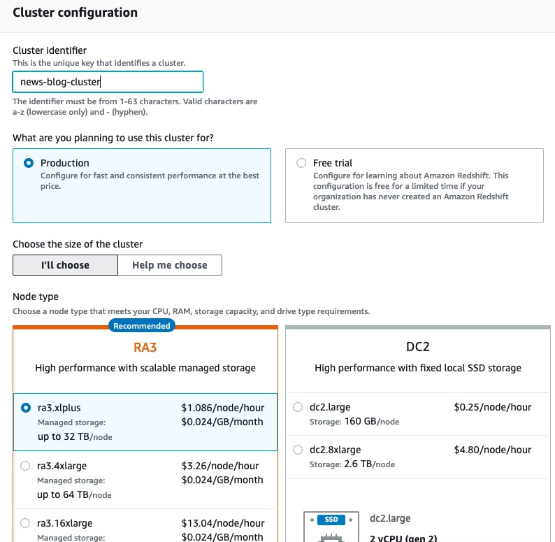
The new RA3.xlplus node provides 4 vCPUs and 32 GiB of RAM and addresses up to 32 TB of managed storage. A cluster with RA3.xlplus node-type can contain up to 32 of these instances, for a total storage of 1024 TB (that’s 1 petabyte!). With the new smaller RA3.xlplus instance type, it’s even easier to get started with Amazon Redshift.

The differences between RA3 nodes are summarized in the following table.

vCPU Memory Storage Quota I/O Price
(US East (N. Virginia))
ra3.xlplus 4 32 GiB 32TB RMS 0.65 GB/sec $1.086 per hour
ra3.4xlarge 12 96 GiB 64TB RMS 2 GB/sec $3.26 per hour
ra3.16xlarge 48 384 GiB 64TB RMS 8 GB/sec $13.04 per hour

Creating a new Amazon Redshift cluster

You can create a new cluster on the Amazon Redshift console or the AWS Command Line Interface (AWS CLI). For this post, I walk you through using the Amazon Redshift console.

  1. On the Amazon Redshift console, choose Clusters.
  2. Choose Create cluster.
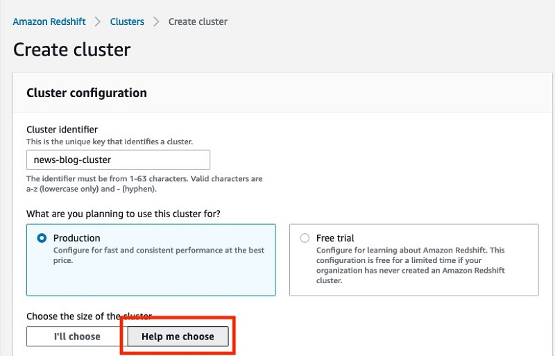
  3. For Choose the size of the cluster, choose I’ll choose.
  4. For Node type, select your preferred node type (for this post, we select xlplus).

The following screenshot shows the Cluster configuration page for the US East (N. Virginia) Region. The price may vary slightly in different Regions.

If you have a DS2 or DC2 instance-based cluster, you can create an RA3 cluster to evaluate the new instance with managed storage. You use a recent snapshot of your Amazon Redshift DS2 or DC2 cluster to create a new cluster based on RA3 instances. We recommend using 2 nodes of RA3.xlplus for every 3 nodes of DS2.xl or 3 nodes of RA3.xlplus for every 8 nodes of DC2.large. For more information about upgrading sizes, see Upgrading to RA3 node types. You can always adjust the compute capacity by adding or removing nodes with elastic resize.

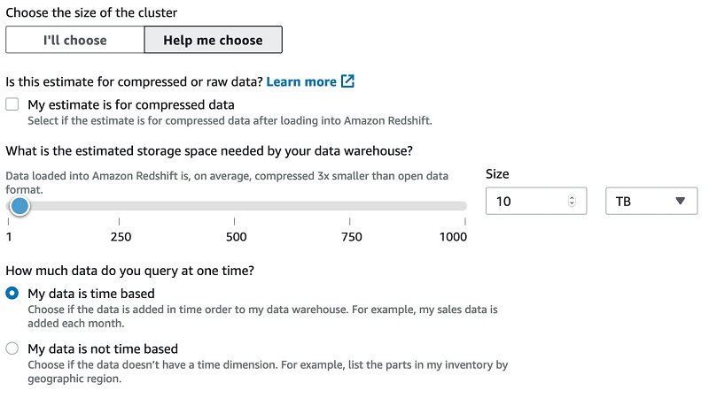
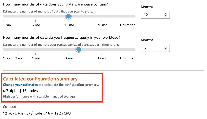
If you’re migrating to Amazon Redshift from on-premises data warehouses, you can size your Amazon Redshift cluster using the sizing widget on the Amazon Redshift console. On the Cluster configuration page, for Choose the size of the cluster, choose Help me choose.

Answer the subsequent questions on total storage size and your data access pattern in order to size your cluster’s compute and storage resource.

The sizing widget recommends the cluster configuration in the Calculated configuration summary section.

Conclusion

RA3 instances are now available in 16 AWS Regions. For the latest RA3 node type availability, see RA3 node type availability in AWS Regions.

The price varies from Region to Region, starting at $1.086 per hour per node in US East (N. Virginia). For more information, see Amazon Redshift pricing.


About the Author

BP Yau is a Data Warehouse Specialist Solutions Architect at AWS. His role is to help customers architect big data solutions to process data at scale. Before AWS, he helped Amazon.com Supply Chain Optimization Technologies migrate its Oracle data warehouse to Amazon Redshift and build its next generation big data analytics platform using AWS technologies.

Amazon EMR Studio (Preview): A new notebook-first IDE experience with Amazon EMR

Post Syndicated from Fei Lang original https://aws.amazon.com/blogs/big-data/amazon-emr-studio-preview-a-new-notebook-first-ide-experience-with-amazon-emr/

We’re happy to announce Amazon EMR Studio (Preview), an integrated development environment (IDE) that makes it easy for data scientists and data engineers to develop, visualize, and debug applications written in R, Python, Scala, and PySpark. EMR Studio provides fully managed Jupyter notebooks and tools like Spark UI and YARN Timeline Service to simplify debugging. EMR Studio uses AWS Single Sign-On (AWS SSO), and allows you to log in directly with your corporate credentials without signing in to the AWS Management Console.

With EMR Studio, you can run notebook code on Amazon EMR running on Amazon Elastic Compute Cloud (Amazon EC2) or Amazon EMR on Amazon Elastic Kubernetes Service (Amazon EKS), and debug your applications. For more information about Amazon EMR on Amazon EKS, see What is Amazon EMR on EKS.

EMR Studio kernels and applications run on EMR clusters, so you get the benefit of distributed data processing with the performance-optimized Apache Spark runtime that Amazon EMR provides. You can also install custom kernels and libraries, collaborate with peers using code repositories such as GitHub and Bitbucket, or run parameterized notebooks as part of scheduled workflows using orchestration services like Apache Airflow or Amazon Managed Workflows for Apache Airflow (Amazon MWAA). Administrators can set up EMR clusters that can be used by EMR Studio users, or create predefined AWS CloudFormation templates for Amazon EMR and allow you to simply choose a template for creating your own cluster.

In this post, we discuss the benefits that EMR Studio offers and we introduce to you some of its capabilities. To learn more about creating and using EMR Studios, see Use Amazon EMR Studio.

Benefits of using EMR Studio

EMR Studio offers the following benefits:

  • Set up a unified experience to develop and diagnose EMR Spark applications – Administrators can set up EMR Studio to allow you to log in using your corporate credentials without having to sign in to the AWS console. You get a single unified environment to interactively explore, process, and visualize data using notebooks, build and schedule pipelines, and debug applications without having to log in to EMR clusters.
  • Use fully managed Jupyter notebooks – With EMR Studio, you can develop analytics and data science applications in R, Python, Scala, and PySpark with fully managed Jupyter notebooks. You can take advantage of distributed processing using the performance-optimized Amazon EMR runtime for Apache Spark with Jupyter kernels and applications running on EMR clusters. you can attach notebooks to an existing cluster that uses Amazon EC2 instances, or to an EMR on EKS virtual cluster. You can also start your own clusters using templates pre-configured by administrators.
  • Collaborate with others using code repositories – From the EMR Studio notebooks environment, you can connect to code repositories such as AWS CodeCommit, GitHub, and Bitbucket to collaborate with peers.
  • Run custom Python libraries and kernels – From EMR Studio, you can install custom Python libraries or Jupyter kernels required for your applications directly to the EMR clusters.
  • Automate workflows using pipelines – EMR Studio makes it easy to move from prototyping to production. You can create EMR Studio notebooks that can be programmatically invoked with parameters, and use APIs to run the parameterized notebooks. You can also use orchestration tools such as Apache Airflow or Amazon MWAA to run notebooks in automated workflows.
  • Simplified debugging – With EMR Studio, you can debug jobs and access logs without logging in to the cluster. EMR Studio provides native application interfaces such as Spark UI and YARN Timeline. When a notebook is run in EMR Studio, the application logs are uploaded to Amazon Simple Storage Service (Amazon S3). As a result, you can access logs and diagnose applications even after your EMR cluster is terminated. You can quickly locate the job to debug by filtering based on the cluster or time when the application was run.

In the following section, we demonstrate some of the capabilities of Amazon EMR Studio using a sample notebook. For our sample notebook, we use the open-source, real-time COVID-19 US daily case reports provided by Johns Hopkins University CSSE from the following GitHub repo.

Notebook-first IDE experience with AWS SSO integration

EMR Studio makes it simple to interact with applications on an EMR cluster. After an administrator sets up EMR Studio and provides the access URL (which looks like https://es-*************************.emrstudio.us-east-1.amazonaws.com), you can log in to EMR Studio with your corporate credentials.

After you log in to EMR Studio, you get started by creating a Workspace. A Workspace is a collection of one or more notebooks for a project. The Workspaces and the notebooks that you create in EMR Studio are automatically saved in an Amazon S3 location.

Now, we create a Workspace by completing the following steps:

  1. On the EMR Studio Dashboard page, choose Create Workspace.
  2. On the Create a Workspace page, enter a Workspace name and a Description.

Naming the Workspace helps identify your project. Your workspace is automatically saved, and you can find it later on the Workspaces page. For this post, we name our Workspace EMR-Studio-WS-Demo1.

  1. On the Subnet drop-down menu, choose a subnet for your Workspace.

Each subnet belongs to the same Amazon Virtual Private Cloud (Amazon VPC) as your EMR Studio. Your administrator may have set up one or more subnets to use for your EMR clusters. You should choose a subnet that matches the subnet where you use EMR clusters. If you’re not sure about which subnet to use, contact your administrator.

  1. For S3 location, choose the Amazon S3 location where EMR Studio backs up all notebook files in the Workspace.

This location is where your Workspace and all the notebooks in the Workspace are automatically saved.

  1. In the Advanced configuration section, you can attach an EMR cluster to your Workspace.

For this post, we skip this step. EMR Studio allows you to create Workspaces and notebooks without attaching to an EMR cluster. You can attach an EMR cluster later when you’re ready to run your notebooks.

  1. Choose Create Workspace.

Fully managed environment for managing and running Jupyter-based notebooks

EMR Studio provides a fully managed environment to help organize and manage Workspaces. Workspaces are the primary building blocks of EMR Studio, and they preserve the state of your notebooks. You can create different Workspaces for each project. From within a Workspace, you can create notebooks, link your Workspace to a code repository, and attach your Workspace to an EMR cluster to run notebooks. Your Workspaces and the notebooks and settings it contains are automatically saved in the Amazon S3 location that you specify.

If you created the workspace EMR-Studio-WS-Demo1 by following the preceding steps, it appears on the Workspaces page with the name EMR-Studio-WS-Demo1 along with status Ready, creation time, and last modified timestamp.

The following table describes each possible Workspace status.

Status Meaning
Starting The Workspace is being prepared, but is not yet ready to use.
Ready You can open the Workspace to use the notebook editor. When a Workspace has a Ready status, you can open or delete it.
Attaching The Workspace is being attached to a cluster.
Attached The Workspace is attached to an EMR cluster. If a Workspace is not attached to an EMR cluster, you need to attach it to an EMR cluster before you can run any notebook code in the Workspace.
Idle

The Workspace is stopped and currently idle. When you launch an idle Workspace, the Workspace status changes from Idle to Starting to Ready.


Stopping The Workspace is being stopped.
Deleting When you delete a Workspace, it’s marked for deletion. EMR Studio automatically deletes Workspaces marked for deletion. After a Workspace is deleted, it no longer shows in the list of Workspaces.

You can choose the Workspace that you created (EMR-Studio-WS-Demo1) to open it. This opens a new web browser tab with the JupyterLab interface. The icon-denoted tabs on the left sidebar allow you to access tool panels such as the file browser or JupyterLab command palette. To learn more about the EMR Studio Workspace interface, see Understand the Workspace User Interface.

EMR Studio automatically creates an empty notebook with the same name as the Workspace. For this post, we the Workspace that we created, it automatically creates EMR-Studio-WS-Demo1.ipynb. In the following screenshot, no cluster or kernel is specified in the top right corner, because we didn’t choose to attach any cluster while creating the Workspace. You can write code in your new notebook, but before you run your code, you need to attach it to an EMR cluster and specify a kernel. To attach your workspace to a cluster, choose the EMR clusters icon on the left panel.

Linking Git-based code repositories with your Workspace

You can collaborate with your peers by sharing notebooks as code via code repositories. EMR Studio supports the following Git-based services:

This capability provides the following benefits:

  • Version control – Record code changes in a version control system so you can review the history of your changes and selectively revert them.
  • Collaboration – Share code with team members working in different Workspaces through remote Git-based repositories. Workspaces can clone or merge code from remote repositories and push changes back to those repositories.
  • Code reuse – Many Jupyter notebooks that demonstrate data analysis or machine learning techniques are available in publicly hosted repositories, such as GitHub. You can associate your Workspace with a GitHub repository to reuse the Jupyter notebooks contained in a repository.

To link Git repositories to your Workspace, you can link an existing repository or create a new one. When you link an existing repository, you choose from a list of Git repositories associated with the AWS account in which your EMR Studio was created.

We add a new repository by completing the following steps:

  1. Choose the Git icon.
  2. For Repository name¸ enter a name (for example, emr-notebook).
  3. For Git repository URL, enter the URL for the Git repo (for this post, we use the sample notebook at https://github.com/emrnotebooks/notebook_execution).
  4. For Git credentials, select your credentials. Because we’re using a public repo, we select Use a public repository without credentials.
  5. Choose Add repository.

After it’s added, we can see the repo on the Git repositories drop-down menu.

  1. Choose the repo to link to the Workspace.

You can link up to three Git repositories with an EMR Studio Workspace. For more information, see Link Git-Based Repositories to an EMR Studio Workspace.

  1. Choose the File browser icon to locate the Git repo we just linked.

Attaching and detaching Workspaces to and from EMR clusters

EMR Studio kernels and applications run on EMR clusters, so you get the benefit of distributed data processing using the performance-optimized EMR runtime for Apache Spark. You can attach your Workspace to an EMR cluster and get distributed data processing using Spark or custom kernels. You can use primary node capacity to run non-distributed applications.

In addition to using Amazon EMR clusters running on Amazon EC2, you can attach a Workspace to an Amazon EMR on EKS virtual cluster to run notebook code. For more information about how to use an Amazon EMR on EKS cluster in EMR Studio, see Use an Amazon EMR on EKS Cluster to Run Notebook Code.

Before you can run your notebooks, you must attach your Workspace to an EMR cluster. For more information about clusters, see Create and Use Clusters with EMR Studio.

To run the Git repo notebooks that we linked in the previous step, complete the following steps:

  1. Choose the EMR cluster
  2. Attach the Workspace to an existing EMR cluster running on Amazon EC2 instances.
  3. Open the notebook demo_pyspark.ipynb from the Git repo emr-notebook that we linked to the Workspace.

In the upper right corner of the Workspace UI, we can see the ID of the EMR cluster being attached to our Workspace, as well as the kernel selected to run the notebook.

  1. Record the value of the cluster ID (for example, <j-*************>).

We use this value later to locate the EMR cluster for application debugging purposes.

You can also detach the Workspace from the cluster in the Workspace UI and re-attach it to another cluster. For more information, see Detach a Cluster from Your Workspace.

Being able to easily attach and detach to and from any EMR cluster allows you to move any workload from prototyping into production. For example, you can start your prototype development by attaching your workspace to a development EMR cluster and working with test datasets. When you’re ready to run your notebook with larger production datasets, you can detach your workspace from the development EMR cluster and attach it to a larger production EMR cluster.

Installing and loading custom libraries and kernels

You can install notebook-scoped libraries with a PySpark kernel in EMR Studio. The libraries installed are isolated to your notebook session and don’t interfere with libraries installed via EMR bootstrap actions, or libraries installed by other EMR Studio notebook sessions that may be running on the same EMR cluster. After you install libraries for your Workspace, they’re available for other notebooks in the Workspace in the same session.

Our sample notebook demo_pyspark.ipynb is a Python script. It uses real-time COVID-19 US daily case reports as input data. The following parameters are defined in the first cell:

  • DATE – The given date used when the notebook job is started.
  • TOP_K – The top k US states with confirmed COVID-19 cases. We use this to plot Graph a.
  • US_STATES – The names of the specific US states being checked for the fatality rates of COVID-19 patients. We use this plot Graph b.

The parameters can be any of the Python data types.

Running this notebook plots two graphs:

  • Graph a – Visualizes the top k US states with most the COVID-19 cases on a given date
  • Graph b – Visualizes the fatality rates among specific US states on a given date

In our notebook, we install notebook-scoped libraries by running the following code from within a notebook cell:

sc.install_pypi_package("pandas==0.25.1")
sc.install_pypi_package("requests==2.24.0")
sc.install_pypi_package("numpy==1.19.1")
sc.install_pypi_package("kiwisolver==1.2.0")
sc.install_pypi_package("matplotlib==3.3.0")

We use these libraries in the subsequent cells for the further data analysis and visualization steps in the notebook.

The following set of parameters is used to run the notebook:

{"DATE": "10-15-2020",
 "TOP_K": 6,
"US_STATES": ["Wisconsin", "Texas", "Nevada"]}

Running all the notebook cells generates two graphs. Graph a shows the top six US states with confirmed COVID-19 cases on October 15, 2020.

Graph b shows the fatality rates of COVID-19 patients in Texas, Wisconsin, and Nevada on October 15, 2020.

EMR Studio also allows you to install Jupyter notebook kernels and Python libraries on a cluster primary node, which makes your custom environment available to any EMR Studio Workspace attached the cluster. To install the sas_kernel kernel on a cluster primary node, run the following code within a notebook cell:

!/emr/notebook-env/bin/pip install sas_kernel

The following screenshot shows your output.

For more information about how to install kernels and use libraries, see Installing and Using Kernels and Libraries.

Diagnosing applications and jobs with EMR Studio

In EMR Studio, you can quickly debug jobs and access logs without logging in to the cluster, such as setting up a web proxy through an SSH connection, for both active and stopped clusters. You can use native application interfaces such as Spark UI and YARN Timeline Service directly from EMR Studio. EMR Studio also allows you to quickly locate the cluster or job to debug by using filters such as cluster state, creation time, and cluster ID. For more information, see Diagnose Applications and Jobs with EMR Studio.

Now, we show you how to open a native application interface to debug the notebook job that already finished.

  1. On the EMR Studio page, choose Clusters.

A list appears with all the EMR clusters launched under the same AWS account. You can filter the list by cluster state, cluster ID, or creation time range by entering values in the provided fields.

  1. Choose the cluster ID of the EMR cluster that we attached to the Workspace EMR-Studio-WS-Demo1 for running notebook demo_pyspark.ipynb.
  2. For Spark job debugging, on the Launch application UIs menu, choose Spark History Server.

The following screenshot shows you the Spark job debugging UI.

We can traverse the details for our notebook application by checking actual logs from the Spark History Server, as in the following screenshot.

  1. For Yarn application debugging, on the Launch application UIs menu, choose Yarn Timeline Server.

The following screenshot shows the Yarn debugging UI.

Orchestrating analytics notebook jobs to build ETL production pipelines

EMR Studio makes it easy for you to move any analytics workload from prototyping to production. With EMR Studio, you can run parameterized notebooks as part of scheduled workflows using orchestration services like AWS Step Functions and Apache Airflow or Amazon MWAA.

In this section, we show a simple example of how to orchestrate running notebook workflows using Apache Airflow.

We have a fully tested notebook under an EMR Studio Workspace, and want to schedule a workflow that runs the notebook on an on-demand EMR cluster every 10 minutes.

Record the value of the Workspace ID (for example, e-*****************************) and the notebook file path relative to the home directory within the Workspace (for example, demo.ipynb or my_folder/demo.ipynb)

The workflow that we create takes care of the following tasks:

  1. Create an EMR cluster.
  2. Wait until the cluster is ready.
  3. Start running a notebook defined by the Workspace ID, notebook file path, and the cluster created.
  4. Wait until the notebook is complete.

The following screenshot is the tree view of this example DAG. The DAG definition is available on the GitHub repo. Make sure you replace any placeholder values with the actual ones before using.

When you open the Gantt chart of one of the successful notebooks, we can see the timeline of our workflow. The time spent creating the cluster and creating a notebook execution is negligible compared to the time spent waiting for the cluster to be ready and waiting for the notebook to finish, which meets the expectation of our SLA.

This example is a just starting point. Try it out and extend it with more sophisticated workflows that suit your needs.

Summary

In this post, we highlighted some of the capabilities of EMR Studio, such as the ability to log in via AWS SSO, access fully managed Jupyter notebooks, link Git-based code repositories, change clusters, load custom Python libraries and kernels, diagnose clusters and jobs using native application UIs, and orchestrate notebook jobs using Apache Airflow or Amazon MWAA.

There is no additional charge for using EMR Studio in public preview, and you only pay for the use of the EMR cluster or other AWS services such as AWS Service Catalog. For more information, see the EMR Studio FAQs.

EMR Studio is available on Amazon EMR release version 6.2 and later, in the US East (N. Virginia), US West (Oregon), and EU (Ireland) Regions for public preview. For the latest Region availability for the public preview, see Considerations.

If you have questions or suggestions, feel free to leave a comment.


About the  Authors

Fei Lang is a Senior Big Data Architect at Amazon Web Services. She is passionate about building the right big data solution for customers. In her spare time, she enjoys the scenery of the Pacific Northwest, going for a swim, and spending time with her family.


Shuang Li is a Senior Product Manager for Amazon EMR at AWS. She holds a doctoral degree in Computer Science and Engineering from Ohio State University.


Ray Liu is a Software Development Engineer at AWS. Besides work, he enjoys traveling and spending time with family.


Kendra Ellis is a Programmer Writer at AWS.
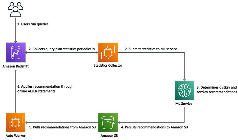


Optimizing tables in Amazon Redshift using Automatic Table Optimization

Post Syndicated from Paul Lappas original https://aws.amazon.com/blogs/big-data/optimizing-tables-in-amazon-redshift-using-automatic-table-optimization/

Amazon Redshift is the most popular and fastest cloud data warehouse that lets you easily gain insights from all your data using standard SQL and your existing business intelligence (BI) tools. Amazon Redshift automates common maintenance tasks and is self-learning, self-optimizing, and constantly adapting to your actual workload to deliver the best possible performance.

Amazon Redshift has several features that automate performance tuning: automatic vacuum delete, automatic table sort, automatic analyze, and Amazon Redshift Advisor for actionable insights into optimizing cost and performance. In addition, automatic workload management (WLM) makes sure that you use cluster resources efficiently, even with dynamic and unpredictable workloads. Amazon Redshift can even automatically refresh and rewrite materialized views, speeding up query performance by orders of magnitude with pre-computed results. These capabilities use machine learning (ML) to adapt as your workloads shift, enabling you to get insights faster without spending valuable time managing your data warehouse.

Although Amazon Redshift provides industry-leading performance out of the box for most workloads, some queries benefit even more by pre-sorting and rearranging how data is physically set up on disk. In Amazon Redshift, you can set the proper sort and distribution keys for tables and allow for significant performance improvements for the most demanding workloads.

Automatic table optimization is a new self-tuning capability that helps you achieve the performance benefits of sort and distribution keys without manual effort. Automatic table optimization continuously observes how queries interact with tables and uses ML to select the best sort and distribution keys to optimize performance for the cluster’s workload. If Amazon Redshift determines that applying a key will improve cluster performance, tables are automatically altered within hours without requiring administrator intervention. Optimizations made by the Automatic table optimization feature have been shown to increase cluster performance by 24% and 34% using the 3 TB and 30 TB TPC-DS benchmark, respectively, versus a cluster without Automatic table optimization.

In this post, we illustrate how you can take advantage of the Automatic table optimization feature for your workloads and easily manage several thousands of tables with zero administration.

Solution overview

The following diagram is an architectural illustration of how Automatic table optimization works:

As you can notice, as users query the data in Amazon Redshift, automatic table optimization collects the query statistics that are analyzed using a machine learning service to predict recommendations about the sort and distribution keys. These recommendations are later applied using online ALTER statements into the respective Amazon Redshift tables automatically.

For this post, we consider a simplified version of the of the star schema benchmark (SSB), which consists of the lineitem fact table along with the part and orders dimensional tables.

We use the preceding dimensional setup to create the tables using the defaults and illustrate how Automatic table optimization can automatically optimize it based on the query patterns.

To try this solution in your AWS account, you need access to an Amazon Redshift cluster and a SQL client such as SQLWorkbench/J. For more information, see Create a sample Amazon Redshift cluster.

Creating SSB tables using the defaults

Let’s start with creating a representative set of tables from the SSB schema and letting Amazon Redshift pick the default settings for the table design.

  1. Create the following tables to set up the dimensional model for the retail system dataset:
    CREATE TABLE orders 
    (
      O_ORDERKEY        BIGINT NOT NULL,
      O_CUSTKEY         BIGINT,
      O_ORDERSTATUS     VARCHAR(1),
      O_TOTALPRICE      DECIMAL(18,4),
      O_ORDERDATE       DATE,
      O_ORDERPRIORITY   VARCHAR(15),
      O_CLERK           VARCHAR(15),
      O_SHIPPRIORITY    INTEGER,
      O_COMMENT         VARCHAR(79)
    );
    CREATE TABLE part 
    (
      P_PARTKEY       BIGINT NOT NULL,
      P_NAME          VARCHAR(55),
      P_MFGR          VARCHAR(25),
      P_BRAND         VARCHAR(10),
      P_TYPE          VARCHAR(25),
      P_SIZE          INTEGER,
      P_CONTAINER     VARCHAR(10),
      P_RETAILPRICE   DECIMAL(18,4),
      P_COMMENT       VARCHAR(23)
    );
    
    CREATE TABLE lineitem 
    (
      L_ORDERKEY        BIGINT NOT NULL,
      L_PARTKEY         BIGINT,
      L_SUPPKEY         BIGINT,
      L_LINENUMBER      INTEGER NOT NULL,
      L_QUANTITY        DECIMAL(18,4),
      L_EXTENDEDPRICE   DECIMAL(18,4),
      L_DISCOUNT        DECIMAL(18,4),
      L_TAX             DECIMAL(18,4),
      L_RETURNFLAG      VARCHAR(1),
      L_LINESTATUS      VARCHAR(1),
      L_SHIPDATE        DATE,
      L_COMMITDATE      DATE,
      L_RECEIPTDATE     DATE,
      L_SHIPINSTRUCT    VARCHAR(25),
      L_SHIPMODE        VARCHAR(10),
      L_COMMENT         VARCHAR(44)
    );
    

    As you can see from the table DDL, apart from the table column definition, no other options are specified. Amazon Redshift defaults the sort key and distribution style to AUTO.

  2. We now load data from the public Amazon Simple Storage Service (Amazon S3) bucket to our new tables. Use any SQL client tool and run the following command, providing your AWS account ID and Amazon Redshift role:
    COPY orders from 's3://salamander-us-east-1/atoblog/orders/' iam_role 'arn:aws:iam::[Your-AWS_Account_Id]:role/[Your-Redshift-Role]'  CSV gzip region 'us-east-1';
    COPY part from 's3://salamander-us-east-1/atoblog/part/' iam_role 'arn:aws:iam::[Your-AWS_Account_Id]:role/[Your-Redshift-Role]'  CSV gzip region 'us-east-1';
    COPY lineitem from 's3://salamander-us-east-1/atoblog/lineitem/' iam_role 'arn:aws:iam::[Your-AWS_Account_Id]:role/[Your-Redshift-Role]'  CSV gzip region 'us-east-1';
    

  3. Wait until the table COPY is complete.

Amazon Redshift automatically assigns the data encoding for the columns and chooses the sort and distribution style based on the size of the table.

  1. Use the following query to review the decisions that Amazon Redshift makes for the column encoding:
    /* Find the column encoding */
    SELECT tablename,
           "column",
           encoding
    FROM pg_table_def
    WHERE tablename = 'lineitem'
    AND   schemaname = 'public' LIMIT 5;
    tablename column encoding
    lineitem	l_orderkey	az64
    lineitem	l_partkey	az64
    lineitem	l_suppkey	az64
    lineitem	l_linenumber	az64
    lineitem	l_quantity	az64
    

  2. Verify the table design choices for the sort and distribution key with the following code:
    SELECT "table",
           diststyle,
           sortkey1
    FROM svv_table_info
    WHERE "table" IN ('part','lineitem','orders')
    table diststyle sortkey1;
    --Output
    part	AUTO(ALL)	AUTO(SORTKEY)
    orders	AUTO(ALL)	AUTO(SORTKEY)
    lineitem	AUTO(EVEN)	AUTO(SORTKEY)

The tables distribution is set to AUTO(EVEN) or AUTO(ALL), depending on the size of table, and sort key is AUTO(SORTKEY).

Until now, because no active workloads were ran against these tables, no specific key choices have been made other than marking them as AUTO.

Querying the SSB tables to emulate the workload

Now end-users can use the created tables, and Amazon Redshift can support out-of-box performance.

The following are some sample queries that we can run using this SSB schema. These queries are run a few repeated times to have Amazon Redshift learn the access patterns for sort and distribution key optimization. To run the query several times, we use the \watch option available with the psql client. Otherwise just run this a few dozen times:

$ psql -h example-corp.cfgio0kcsmjy.us-west-2.redshift.amazonaws.com -U awsuser -d dw -p 5492
dw=# # \timing on
Timing is on.
--turn off result set cache so that each query execution is counted towards a workload sample

dw=# set enable_result_cache_for_session to off;
SET
dw=# /* query 1 */ SELECT L_SHIPMODE,SUM(l_quantity) AS quantity FROM lineitem JOIN part ON P_PARTKEY = l_PARTKEY where L_SHIPDATE='1992-02-28' GROUP BY L_SHIPMODE;
 l_shipmode |  quantity   
------------+-------------
 MAIL       | 436272.0000
 FOB        | 440959.0000
Time: 10020.200 ms
dw=# \watch 2
dw=# /* query 2 */ SELECT COUNT(o_orderkey) AS orders_count, SUM(l_quantity) AS quantity FROM lineitem JOIN orders ON l_orderkey = o_orderkey WHERE L_SHIPDATE = '1992-02-29'
Time: 8932.200 ms
dw=# \watch 2

The preceding queries are run a few hundred times every 2 seconds, and you can press Ctrl+C to cancel the queries.

Alternatively, you can also use the query editor to schedule the query and run it multiple times.

Reviewing recommended sort and distribution keys

Automatic table optimization uses Amazon Redshift Advisor sort and distribution key recommendations. The Advisor continuously monitors the cluster’s workload and proposes the right sort and distribution keys to improve query speed. With Automatic Table Optimization, the Advisor recommendations are visible in the SVV_ALTER_TABLE_RECOMMENDATIONS system table. This view shows recommendations for all tables, whether or not they are defined for automatic optimization. Recommendations that have auto_eligible = False are not automatically applied, but you can run the DDL to apply the recommendation manually. See the following code:

select * from svv_alter_table_recommendations
type      | database | table_id | group_id | ddl                                                                                                                                                 | auto_eligible
diststyle | db0      | 117892   | 2        | ALTER TABLE /*dkru-558bc9ee-468a-457a-99a9-e73ee7da1a18-g0-0*/ "public"."orders" ALTER DISTSTYLE KEY DISTKEY "o_orderkey" SORT                                                                               | t
 diststyle | db0      | 117885   | 1        | ALTER TABLE /*dkru-558bc9ee-468a-457a-99a9-e73ee7da1a18-g0-1*/ "public"."lineitem" ALTER DISTSTYLE KEY DISTKEY "l_orderkey" SORT| t
 sortkey   | db0      | 117890   | -1       | ALTER TABLE /*skru-15a98513-cf0f-46e8-b454-8bf61ee30c6e-g0-0*/ "public"."lineitem" ALTER SORTKEY ("l_shipdate");|t                

Applying recommendations to the target tables

Amazon Redshift takes advantage of the new Automatic table optimization feature to apply the optimization made by the Advisor to the target tables. The conversion is run by the automation during periods of low workload intensity so as to minimize impact on user queries. This can be verified by running the following query:

SELECT "table",
       diststyle,
       sortkey1
FROM svv_table_info
WHERE "table" IN ('part','lineitem','orders')
AND   SCHEMA = 'public';
table,diststyle,sortkey1
part	AUTO(EVEN)	AUTO(SORTKEY)
lineitem	AUTO(KEY(l_orderkey))	AUTO(SORTKEY(l_shipdate)) 
orders	AUTO(KEY(o_orderkey))	AUTO(SORTKEY)

You can view all the optimizations that are applied on the tables using the following query:

select * from svl_auto_worker_action 
1395658	sortkey	Start                                                                                                                           	2020-10-27 22:37:23.367456	0	                                                                                                                                                                                                        
1395658	sortkey	Complete                                                                                                                        	2020-10-27 22:37:23.936958	0	SORTKEY: None;                                                                                                                                                                 

Amazon Redshift can self-learn based on the workload, learn from the table access patterns, and apply the table design optimizations automatically.

Now let’s run the sample workload queries again after optimization:

$ psql -h example-corp.cfgio0kcsmjy.us-west-2.redshift.amazonaws.com -U awsuser -d dw -p 5492
dw=# # \timing on
Timing is on.
--turn off result set cache so that each query is executed as if executed first time
dw=# set enable_result_cache_for_session to off;
SET
dw=# /* query 1 */ SELECT L_SHIPMODE,SUM(l_quantity) AS quantity FROM lineitem JOIN part ON P_PARTKEY = l_PARTKEY where L_SHIPDATE='1992-02-28' GROUP BY L_SHIPMODE;
 l_shipmode |  quantity   
------------+-------------
 MAIL       | 436272.0000
 FOB        | 440959.0000
Time: 4020.900 ms
dw=# /* query 2 */ SELECT COUNT(o_orderkey) AS orders_count, SUM(l_quantity) AS quantity FROM lineitem JOIN orders ON l_orderkey = o_orderkey WHERE L_SHIPDATE = '1992-02-29'
Time: 3532.200 ms

With the sort and distribution optimization, query 1 and query 2 run with 40% less time elapsed, also shown by the following visual.

Converting existing tables for optimization

You can easily convert existing tables for Automatic table optimization using the ALTER table command and switch the sort and distribution styles to AUTO so that it can be automatically optimized by Amazon Redshift. See the following code:

/* Convert a table to a diststyle AUTO table */
ALTER TABLE <tbl> ALTER DISTSTYLE AUTO; 
/* Convert  table to a sort key AUTO table */
ALTER TABLE <tbl> ALTER SORTKEY AUTO; 

Lead time to apply the recommendation

Amazon Redshift continuously learns from workloads, and optimizations are inserted into the svv_alter_table_recomendations. When an optimization is available, it runs within a defined frequency, as well as in periods of low workload intensity, so as to minimize impact on user queries. For more information about the lead time of applying the recommendation, see  https://docs.aws.amazon.com/redshift/latest/dg/t_Creating_tables.html

Conclusion

Automatic table optimization for Amazon Redshift is a new capability that applies sort and distribution keys without the need for administrator intervention. Using automation to tune the design of tables lets you get started more easily and decreases the amount of administrative effort. Automatic table optimization enables easy management of large numbers of tables in a data warehouse because Amazon Redshift self-learns, self-optimizes, and adapts to your actual workload to deliver you the best possible performance.


About the Author

Paul Lappas is a Principal Product Manager at Amazon Redshift.  Paul is responsible for Amazon Redshift’s self-tuning capabilities including Automatic Table Optimization, Workload Manager, and the Amazon Redshift Advisor. Paul is passionate about helping customers leverage their data to gain insights and make critical business decisions. In his spare time Paul enjoys playing tennis, cooking, and spending time with his wife and two boys.


Thiyagarajan Arumugam is a Principal Solutions Architect at Amazon Web Services and designs customer architectures to process data at scale. Prior to AWS, he built data warehouse solutions at Amazon.com. In his free time, he enjoys all outdoor sports and practices the Indian classical drum mridangam.


KamCheung Ting is a Senior Software Engineer at Amazon Redshift. He joined Redshift in 2014 and specializes in storage engine, autonomous DB and concurrency scaling.
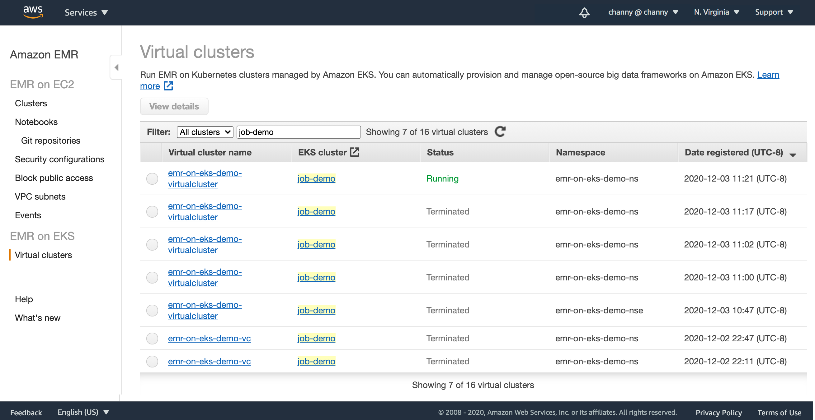
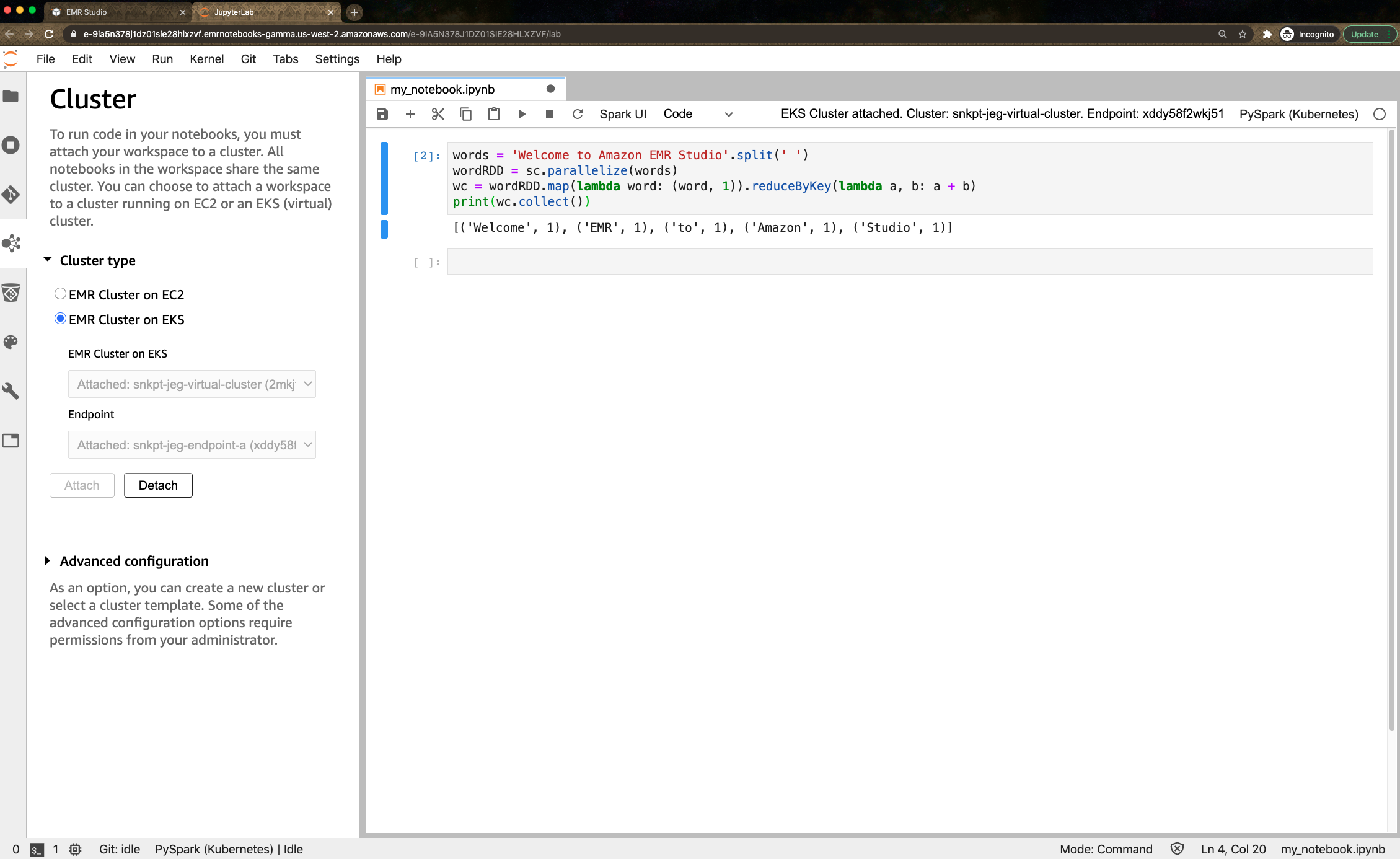


New – Amazon EMR on Amazon Elastic Kubernetes Service (EKS)

Post Syndicated from Channy Yun original https://aws.amazon.com/blogs/aws/new-amazon-emr-on-amazon-elastic-kubernetes-service-eks/

Tens of thousands of customers use Amazon EMR to run big data analytics applications on frameworks such as Apache Spark, Hive, HBase, Flink, Hudi, and Presto at scale. EMR automates the provisioning and scaling of these frameworks and optimizes performance with a wide range of EC2 instance types to meet price and performance requirements. Customer are now consolidating compute pools across organizations using Kubernetes. Some customers who manage Apache Spark on Amazon Elastic Kubernetes Service (EKS) themselves want to use EMR to eliminate the heavy lifting of installing and managing their frameworks and integrations with AWS services. In addition, they want to take advantage of the faster runtimes and development and debugging tools that EMR provides.

Today, we are announcing the general availability of Amazon EMR on Amazon EKS, a new deployment option in EMR that allows customers to automate the provisioning and management of open-source big data frameworks on EKS. With EMR on EKS, customers can now run Spark applications alongside other types of applications on the same EKS cluster to improve resource utilization and simplify infrastructure management.

Customers can deploy EMR applications on the same EKS cluster as other types of applications, which allows them to share resources and standardize on a single solution for operating and managing all their applications. Customers get all the same EMR capabilities on EKS that they use on EC2 today, such as access to the latest frameworks, performance optimized runtimes, EMR Notebooks for application development, and Spark user interface for debugging.

Amazon EMR automatically packages the application into a container with the big data framework and provides pre-built connectors for integrating with other AWS services. EMR then deploys the application on the EKS cluster and manages logging and monitoring. With EMR on EKS, you can get 3x faster performance using the performance-optimized Spark runtime included with EMR compared to standard Apache Spark on EKS.

Amazon EMR on EKS – Getting Started
If you already have a EKS cluster where you run Spark jobs, you simply register your existing EKS cluster with EMR using the AWS Management Console, AWS Command Line Interface (CLI) or APIs to deploy your Spark appication.

For exampe, here is a simple CLI command to register your EKS cluster.

$ aws emr create-virtual-cluster \
          --name <virtual_cluster_name> \
          --container-provider '{
             "id": "<eks_cluster_name>",
             "type": "EKS",
             "info": {
                 "eksInfo": {
                     "namespace": "<namespace_name>"
                 }
             } 
         }'

In the EMR Management console, you can see it in the list of virtual clusters.

When Amazon EKS clusters are registered, EMR workloads are deployed to Kubernates nodes and pods to manage application execution and auto-scaling, and sets up managed endpoints so that you can connect notebooks and SQL clients. EMR builds and deploys a performance-optimized runtime for the open source frameworks used in analytics applications.

You can simply start your Spark jobs.

$ aws emr start-job-run \
          --name <job_name> \
          --virtual-cluster-id <cluster_id> \
          --execution-role-arn <IAM_role_arn> \
          --virtual-cluster-id <cluster_id> \
          --release-label <<emr_release_label> \
          --job-driver '{
            "sparkSubmitJobDriver": {
              "entryPoint": <entry_point_location>,
              "entryPointArguments": ["<arguments_list>"],
              "sparkSubmitParameters": <spark_parameters>
            }
       }'

To monitor and debug jobs, you can use inspect logs uploaded to your Amazon CloudWatch and Amazon Simple Storage Service (S3) location configured as part of monitoringConfiguration. You can also use the one-click experience from the console to launch the Spark History Server.

Integration with Amazon EMR Studio

Now you can submit analytics applications using AWS SDKs and AWS CLI, Amazon EMR Studio notebooks, and workflow orchestration services like Apache Airflow. We have developed a new Airflow Operator for Amazon EMR on EKS. You can use this connector with self-managed Airflow or by adding it to the Plugin Location with Amazon Managed Workflows for Apache Airflow.

You can also use newly previewed Amazon EMR Studio to perform data analysis and data engineering tasks in a web-based integrated development environment (IDE). Amazon EMR Studio lets you submit notebook code to EMR clusters deployed on EKS using the Studio interface. After seting up one or more managed endpoints to which Studio users can attach a Workspace, EMR Studio can communicate with your virtual cluster.

For EMR Studio preview, there is no additional cost when you create managed endpoints for virtual clusters. To learn more, visit the guide document.

Now Available
Amazon EMR on Amazon EKS is available in US East (N. Virginia), US West (Oregon), and Europe (Ireland) Regions. You can run EMR workloads in AWS Fargate for EKS removing the need to provision and manage infrastructure for pods as a serverless option.

To learn more, visit the documentation. Please send feedback to the AWS forum for Amazon EMR or through your usual AWS support contacts.

Learn all the details about Amazon EMR on Amazon EKS and get started today.

Channy;

Announcing Amazon Redshift data sharing (preview)

Post Syndicated from Neeraja Rentachintala original https://aws.amazon.com/blogs/big-data/announcing-amazon-redshift-data-sharing-preview/

Amazon Redshift is a fast, scalable, secure, and fully managed cloud data warehouse that makes it simple and cost-effective to analyze all your data using standard SQL. Amazon Redshift offers up to 3x better price performance than any other cloud data warehouse. Tens of thousands of customers use Amazon Redshift to process exabytes of data per day and power analytics workloads such as high-performance business intelligence (BI) reporting, dashboarding applications, data exploration, and real-time analytics.

We’re excited to launch the new Amazon Redshift data sharing capability, which enables you to securely and easily share live data across Amazon Redshift clusters. Data sharing allows you to extend the ease of use, performance, and cost benefits that Amazon Redshift offers in a single cluster to multi-cluster deployments while being able to share data. Data sharing enables instant, granular, and high-performance data access across Amazon Redshift clusters without the need to copy or move it. Data sharing provides live access to data so that your users always see the most up-to-date and consistent information as it’s updated in the data warehouse. There is no additional cost to use data sharing on your Amazon Redshift clusters.

In this post, we discuss the needs for data sharing in organizations, current challenges when it comes to sharing data, and how Amazon Redshift data sharing addresses these needs.

Need for sharing data in organizations and current challenges

We hear from our customers that they want to share data at many levels to enable broad and deep insights but also minimize complexity and cost. For example, data needs to be shared from a central data warehouse that loads and transforms constant streams of updates with BI and analytics clusters that serve a variety of workloads, such as dashboarding applications, ad-hoc queries, and data science. Multiple teams and business groups within an organization want to share and collaborate on data to gain differentiated insights that can help unlock new market opportunities, or analyze cross-group impact. As data becomes more valuable, many organizations are becoming data providers too and want to share data across organizations and offer analytics services to external consumers.

Before the launch of Amazon Redshift data sharing, in order to share data, you needed to unload data from one system (the producer) and copy it into another (the consumer). This approach can be expensive and introduce delays, especially as the number of consumers grow. It requires building and maintaining separate extract, transform, and load (ETL) jobs to provide relevant subsets of the data for each consumer. The complexity increases with the security practices that must be kept in place to regularly monitor business-critical data usage and ensure compliance. Additionally, this way of sharing doesn’t provide users with complete and up-to-date views of the data and limits insights. Organizations want a simple and secure way to share fresh, complete, and consistent views of data with any number of consumers.

Introduction to Amazon Redshift data sharing

Amazon Redshift data sharing allows you to securely and easily share data for read purposes across different Amazon Redshift clusters without the complexity and delays associated with data copies and data movement. Data can be shared at many levels, including schemas, tables, views, and user-defined functions, providing fine-grained access controls that can be tailored for different users and businesses that all need access to the data.

Consumers can discover shared data using standard SQL interfaces and query it with high performance from familiar BI and analytics tools. Users connect to an Amazon Redshift database in their cluster, and can perform queries by referring to objects from any other Amazon Redshift database that they have permissions to access, including the databases shared from remote clusters. Amazon Redshift enables sharing live and transactionally consistent views of the data, meaning that consumers always view the most up-to-date data, even when it’s continuously updated on the producer clusters. Amazon Redshift clusters that share data can be in the same or different AWS accounts, making it possible for you to share data across organizations and collaborate with external parties in a secure and governed manner. Amazon Redshift offers comprehensive auditing capabilities using system tables and AWS CloudTrail to allow you to monitor the data sharing permissions and the usage across all the consumers and revoke access instantly, when necessary.

Data sharing provides high-performance access and workload isolation

Data sharing builds on Amazon Redshift RA3 managed storage, which decouples storage and compute, allowing either of them to scale independently. With data sharing, workloads accessing shared data are isolated from each other. Queries accessing shared data run on the consumer cluster and read data from the Amazon Redshift managed storage layer directly without impacting the performance of the producer cluster.

You can now rapidly onboard any number of workloads with diverse data access patterns and SLA requirements and not be concerned about resource contention. Workloads accessing shared data can be provisioned with flexible compute resources that meet their workload-specific price performance requirements and be scaled independently as needed in a self-service fashion. You can optionally allow these teams and business groups to pay for what they use with charge-back. With data sharing, the producer cluster pays for the managed storage cost of the shared data, and the consumer cluster pays for the compute. Data sharing itself doesn’t have any cost associated with it.

Consumer clusters are regular Amazon Redshift clusters. Although consumer clusters can only read the shared data, they can write their own private data and if desired, share it with other clusters, including back to the producer cluster. Building on a managed storage foundation also enables high-performance access to the data. The frequently accessed datasets are cached on the local compute nodes of the consumer cluster to speed up those queries. The following diagram illustrates this data sharing architecture.

How data sharing works

Data sharing between Amazon Redshift clusters is a two-step process. First, the administrator of the producer cluster that wants to share data creates a data share, a new named object that serves as a unit of sharing. The administrator of the producer cluster and other privileged users add the needed database objects such as schemas, tables, views (regular, late binding, and materialized) to the data share and specify a list of consumers for sharing purposes. Consumers can be other Amazon Redshift clusters in the same AWS account or separate AWS accounts.

Next, the administrator of the consumer cluster looks at the shared datasets and reviews the contents of each share. To consume shared data, the consumer cluster administrator creates an Amazon Redshift database from the data share object and assigns permissions to appropriate users and groups in the consumer cluster. Users and groups that have access to shared data can discover and query it using standard SQL and analytics tools. You can join shared data with local data and perform cross-database queries. We have introduced new metadata views and modified JDBC/ODBC drivers so that tools can seamlessly integrate with shared data. The following diagram illustrates this data sharing architecture.

Data sharing use cases

In this section, we discuss the common data sharing use cases:

  • Sharing data from a central ETL cluster with multiple, isolated BI and analytics clusters in a hub-spoke architecture to provide read workload isolation and optional charge-back for costs.
  • Sharing data among multiple business groups so they can collaborate for broader analytics and data science. Each Amazon Redshift cluster can be a producer of some data but also can be a consumer of other datasets.
  • Sharing data in order to offer data and analytics as a service across the organization and with external parties.
  • Sharing data between development, test, and production environments, at any granularity.

Amazon Redshift offers unparalleled compute flexibility

Amazon Redshift offers you the most flexibility than any other cloud data warehouse when it comes to organizing your workloads based on price performance, isolation, and charge-ability. Amazon Redshift efficiently utilizes compute resources in a cluster to maximize performance and throughput with automatic workload management (WLM). Specifying query priorities allows you to influence the usage of resources across multiple workloads based on business priorities. With Amazon Redshift concurrency scaling, you can elastically scale one or more workloads in a cluster automatically with extra capacity to handle high concurrency and query spikes without any application changes. And with data sharing, you can now handle diverse business-critical workloads that need flexible compute resources, isolation, and charge-ability with multi-cluster deployments while sharing data. You can use WLM and concurrency scaling on both data sharing producer and consumer clusters.

The combination of these capabilities allows you to evolve from single cluster to multi-cluster deployments easily and cost-efficiently.

Beyond sharing data across Amazon Redshift clusters

Along with sharing data across Amazon Redshift clusters, our vision is to evolve data sharing so you can share Amazon Redshift data with the Amazon Simple Storage Service (Amazon S3) data lake by publishing data shares to the AWS Lake Formation catalog. This enables other AWS analytics services to discover and access live and transactionally consistent data in Amazon Redshift managed storage. For example, you could incorporate live data from Amazon Redshift in an Amazon EMR Spark data pipeline, perform ad-hoc queries on Amazon Redshift data using Amazon Athena, or use clean and curated data in Amazon Redshift to build machine learning models with Amazon SageMaker. The following diagram illustrates this architecture.

Amazon Redshift data sharing in customer environments

Data sharing across Amazon Redshift clusters within the same account is now available for preview. Sharing across clusters that are in different AWS accounts is coming soon. We worked closely with several customers and partners for an early preview of data sharing and they are excited about the results and possibilities.

“At Warner Bros. Games, we build and maintain complex data mobility infrastructures to manage data movements across single game clusters and consolidated business function clusters. However, developing and maintaining this system monopolizes valuable team resources and introduces delays that impede our ability to act on the data with agility and speed. Using the Redshift data sharing feature, we can remove the entire subsystem we built for data copying, movement, and loading between Redshift clusters. This will empower all of our business teams to make decisions on the right datasets more quickly and efficiently. Additionally, Redshift data sharing will also allow us to re-architect compute provisioning to more closely align with the resources needed to execute those functions’ SQL workloads—ultimately enabling simpler infrastructure operations.”

— Kurt Larson, Technical Director, Warner Bros. Analytics

“The data sharing feature seamlessly allows multiple Redshift clusters to query data located in our RA3 clusters and their managed storage. This eliminates our concerns with delays in making data available for our teams, and reduces the amount of data duplication and associated backfill headache. We now can concentrate even more of our time making use of our data in Redshift and enable better collaboration instead of data orchestration.”

— Steven Moy, Engineer, Yelp

“At Fannie Mae, we adopted a de-centralized approach to data warehouse management with tens of Amazon Redshift clusters across many applications. While each team manages their own dataset, we often have use cases where an application needs to query the datasets from other applications and join with the data available locally. We currently unload and move data from one cluster to another cluster, and this introduces delays in providing timely access to data to our teams. We have had issues with unload operations spiking resource consumption on producer clusters, and data sharing allows us to skip this intermediate unload to Amazon S3, saving time and lowering consumption. Many applications are performing unloads currently in order to share datasets, and we plan to convert all such processes to leveraging the new data sharing feature. With data sharing, we can enable seamless sharing of data across application teams and give them common views of data without having to do ETL. We are also able to avoid the data copies between pre-prod, research, and production environments for each application. Data sharing made us more agile and gave us the flexibility to scale analytics in highly distributed environments like Fannie Mae.”

— Amy Tseng, Enterprise Databases Manager, Fannie Mae

“Shared storage allowed us to focus on what matters: making data available to end-users. Data is no longer stuck in a myriad of storage mediums or formats, or accessible only through select APIs, but rather in a single flavor of SQL.”

— Marco Couperus, Engineering Manager, home24

“We’re excited to launch our integration with Amazon Redshift data sharing, which is a game changer for analytics teams that are looking to improve analytics performance SLAs and reduce data processing delays for diverse workloads across organizations. By isolating workloads that have different access patterns, different SLA requirements such as BI reporting, dashboarding applications, ETL jobs, and data science workloads into separate clusters, customers will now get more control over compute resources and more predictability in their workload SLAs while still sharing common data. The integrations of Etleap with Amazon Redshift data sharing will make sharing data between clusters seamless as part of their existing data pipelines. We are thrilled to offer this integrated experience to our joint customers.”

— Christian Romming, Founder and CEO, Etleap

“We’re excited to partner with AWS to enable data sharing for Amazon Redshift within Aginity Pro. Amazon Redshift users can now navigate and explore shared data within Aginity products just like local data within their clusters. Users can then build reusable analytics that combine both local and shared data seamlessly using cross-database queries. Importantly, shared data query performance has the same high performance as local queries without the cost and performance penalty of traditional federation solutions. We’re thrilled to see how our customers will leverage the ability to securely share data across clusters.”

— Matthew Mullins, CTO, Aginity

Next steps

The preview for within account data sharing is available on Amazon Redshift RA3 node types in the following regions:

  • US East (Ohio)
  • US East (N. Virginia)
  • US West (N. California)
  • US West (Oregon)
  • Asia Pacific (Seoul)
  • Asia Pacific (Sydney)
  • Asia Pacific (Tokyo)
  • Europe (Frankfurt)
  • Europe (Ireland)

For more information about how to get started with the preview, see documentation.


About the Authors

 Neeraja Rentachintala is a principal product manager with Amazon Web Services who is focused on building Amazon Redshift – the world’s most popular, highest performing, and most scalable cloud data warehouse. Neeraja earned a Bachelor of Technology in Electronics and Communication Engineering from the National Institute of Technology in India and various business program certifications from the University of Washington, MIT Sloan School of Management, and Stanford University.


Ippokratis Pandis is a senior principal engineer at AWS. Ippokratis leads initiatives in AWS analytics and data lakes, especially in Amazon Redshift. He holds a Ph.D. in electrical engineering from Carnegie Mellon University.


Naresh Chainani is a senior software development manager with Amazon Redshift, where he leads Query Processing, Query Performance, Distributed Systems, and Workload Management with a strong team. He is passionate about building high-performance databases to enable customers to gain timely insights and make critical business decisions. In his spare time, Naresh enjoys reading and playing tennis.



Security updates for Wednesday

Post Syndicated from original https://lwn.net/Articles/839481/rss

Security updates have been issued by Debian (golang-golang-x-net-dev, python-certbot, and xorg-server), Fedora (resteasy, scap-security-guide, and vips), openSUSE (chromium, python, and rpmlint), SUSE (kernel), and Ubuntu (aptdaemon, curl, gdk-pixbuf, lxml, and openssl, openssl1.0).

Cloudflare’s privacy-first Web Analytics is now available for everyone

Post Syndicated from Jon Levine original https://blog.cloudflare.com/privacy-first-web-analytics/

Cloudflare’s privacy-first Web Analytics is now available for everyone

Cloudflare’s privacy-first Web Analytics is now available for everyone

In September, we announced that we’re building a new, free Web Analytics product for the whole web. Today, I’m excited to announce that anyone can now sign up to use our new Web Analytics — even without changing your DNS settings. In other words, Cloudflare Web Analytics can now be deployed by adding an HTML snippet (in the same way many other popular web analytics tools are) making it easier than ever to use privacy-first tools to understand visitor behavior.

Why does the web need another analytics service?

Popular analytics vendors have business models driven by ad revenue. Using them implies a bargain: they track visitor behavior and create buyer profiles to retarget your visitors with ads; in exchange, you get free analytics.

At Cloudflare, our mission is to help build a better Internet, and part of that is to deliver essential web analytics to everyone with a website, without compromising user privacy. For free. We’ve never been interested in tracking users or selling advertising. We don’t want to know what you do on the Internet — it’s not our business.

Our customers have long relied on Cloudflare’s Analytics because we’re accurate, fast, and privacy-first. In September we released a big upgrade to analytics for our existing customers that made them even more flexible.

However, we know that there are many folks who can’t use our analytics, simply because they’re not able to onboard to use the rest of Cloudflare for Infrastructure — specifically, they’re not able to change their DNS servers. Today, we’re bringing the power of our analytics to the whole web. By adding a simple HTML snippet to your website, you can start measuring your web traffic — similar to other popular analytics vendors.

What can I do with Cloudflare Web Analytics?

We’ve worked hard to make our analytics as powerful and flexible as possible — while still being fast and easy to use.

When measuring analytics about your website, the most common questions are “how much traffic did I get?” and “how many people visited?” We answer this by measuring page views (the total number of times a page view was loaded) and visits (the number of times someone landed on a page view from another website).

With Cloudflare Web Analytics, it’s easy to switch between measuring page views or visits. Within each view, you can see top pages, countries, device types and referrers.

Cloudflare’s privacy-first Web Analytics is now available for everyone

My favorite thing is the ability to add global filters, and to quickly drill into the most important data with actions like “zoom” and “group by”. Say you publish a new blog post, and you want to see the top sites that send you traffic right after you email your subscribers about it. It’s easy to zoom into the time period when you hit the email, and group by to see the top pages. Then you can add a filter to just that page — and then finally view top referrers for that page. It’s magic!

Best of all, our analytics is free. We don’t have limits based on the amount of traffic you can send it. Thanks to our ABR technology, we can serve accurate analytics for websites that get anywhere from one to one billion requests per day.

How does the new Web Analytics work?

Traditionally, Cloudflare Analytics works by measuring traffic at our edge. This has some great benefits; namely, it catches all traffic, even from clients that block JavaScript or don’t load HTML. At the edge, we can also block bots, add protection from our WAF, and measure the performance of your origin server.

The new Web Analytics works like most other measurement tools: by tracking visitors on the client. We’ve long had client-side measuring tools with Browser Insights, but these were only available to orange-cloud users (i.e. Cloudflare customers).

Today, for the first time, anyone can get access to our client-side analytics — even if you don’t use the rest of Cloudflare. Just add our JavaScript snippet to any website, and we can start collecting metrics.

How do I sign up?

We’ve worked hard making our onboarding as simple as possible.

First, enter the name of your website. It’s important to use the domain name that your analytics will be served on — we use this to filter out any unwanted “spam” analytics reports.

Cloudflare’s privacy-first Web Analytics is now available for everyone

(At this time, you can only add analytics from one website to each Cloudflare account. In the coming weeks we’ll add support for multiple analytics properties per account.)

Next, you’ll see a script tag that you can copy onto your website. We recommend adding this just before the closing </body> tag on the pages you want to measure.

Cloudflare’s privacy-first Web Analytics is now available for everyone

And that’s it! After you release your website and start getting visits, you’ll be able to see them in analytics.

What does privacy-first mean?

Being privacy-first means we don’t track individual users for the purposes of serving analytics. We don’t use any client-side state (like cookies or localStorage) for analytics purposes. Cloudflare also doesn’t track users over time via their IP address, User Agent string, or any other immutable attributes for the purposes of displaying analytics — we consider “fingerprinting” even more intrusive than cookies, because users have no way to opt out.

The concept of a “visit” is key to this approach. Rather than count unique IP addresses, which would require storing state about what each visitor does, we can simply count the number of page views that come from a different site. This provides a perfectly usable metric that doesn’t compromise on privacy.

Cloudflare’s privacy-first Web Analytics is now available for everyone

What’s next

This is just the start for our privacy-first Analytics. We’re excited to integrate more closely with the rest of Cloudflare, and give customers even more detailed stats about performance and security (not just traffic.) We’re also hoping to make our analytics even more powerful as a standalone product by building support for alerts, real-time time updates, and more.

Please let us know if you have any questions or feedback, and happy measuring!

Gifts that last all year round

Post Syndicated from Ashley Whittaker original https://www.raspberrypi.org/blog/gifts-that-last-all-year-round/

What if you could give the joy of opening a Raspberry Pi–themed gift every single month for a whole year? But what if the thought of wrapping 12 individual things fills you with Scrooge-level dread?

Snap up a magazine subscription for one of your nearest and/or dearest and we’ll take care of the packaging and delivery while you sit back and reap all the credit!

You could end up with a few extra gifts depending on what you sign up for so, read on and take your pick.

The MagPi magazine

Magpi magazines fanned out with free gift to the side of them

The official Raspberry Pi magazine comes with a free Raspberry Pi Zero W kit worth £20 when you sign up for a 12-month subscription. You can use our tiniest computer in tonnes of projects, meaning Raspberry Pi fans can never have enough. That’s a top gift-giving bonus for you right there.

Every issue of The MagPi is packed with computing and electronics tutorials, how-to guides, and the latest news and reviews. They also hit their 100th issue this month so, if someone on your list has been thinking about getting a subscription, now is a great time.

Check out subscription deals on the official Raspberry Pi Press store.

HackSpace magazine

Hackspace magazines fanned out with adafruit gift on top

HackSpace magazine is the one to choose for fixers and tinkerers of all abilities. If you’re looking for a gift for someone who is always taking things apart and hacking everyday objects, HackSpace magazine will provide a year of inspiration for them.

12-month subscriptions come with a free Adafruit Circuit Playground Express, which has been specially developed to teach programming novices from scratch and is worth £25.

Check out subscription deals on the official Raspberry Pi Press store.

Custom PC

Some Custom PC magazines fanned out with the free giveaway mouse on top of them

Custom PC is the magazine for people who are passionate about PC technology and hardware. And they’ve just launched a pretty cool new giveaway with every 12-month subscription: a free Chillblast Aero RGB Gaming mouse worth £40. Look, it lights up, it’s cool.

Check out subscription offers on the official Raspberry Pi Press store.

Wireframe magazine

Wireframe magazine lifts the lid on video games. In every issue, you’ll find out how games are made, who makes them, and how you can code them to play for yourself using detailed guides.

The latest deal gets you three issues for just £10, plus your choice of one of our official books as a gift. By the way, that ‘three for £10 plus a free book’ is available across ALL our magazines. Did I not tell you that before? My bad. It’s good though, right?

Check out more subscriptions deals on the official Raspberry Pi Press store.

Three books for the price of one

A selection of Raspberry Pi books on a table surrounded by Christmas decorations

And as an extra Christmas gift to you all, we’ve decided to keep our Black Friday deal rolling until Christmas Eve, so if you buy just one teeny tiny book from the Raspberry Pi Press store, you get two more completely FREE!

Better still, all of the books in the deal only cost £7 or £10 to start with, so makes for a good chunky batch of presents at a brilliantly affordable price.

The post Gifts that last all year round appeared first on Raspberry Pi.

FireEye Hacked

Post Syndicated from Bruce Schneier original https://www.schneier.com/blog/archives/2020/12/fireeye-hacked.html

FireEye was hacked by — they believe — “a nation with top-tier offensive capabilities”:

During our investigation to date, we have found that the attacker targeted and accessed certain Red Team assessment tools that we use to test our customers’ security. These tools mimic the behavior of many cyber threat actors and enable FireEye to provide essential diagnostic security services to our customers. None of the tools contain zero-day exploits. Consistent with our goal to protect the community, we are proactively releasing methods and means to detect the use of our stolen Red Team tools.

We are not sure if the attacker intends to use our Red Team tools or to publicly disclose them. Nevertheless, out of an abundance of caution, we have developed more than 300 countermeasures for our customers, and the community at large, to use in order to minimize the potential impact of the theft of these tools.

We have seen no evidence to date that any attacker has used the stolen Red Team tools. We, as well as others in the security community, will continue to monitor for any such activity. At this time, we want to ensure that the entire security community is both aware and protected against the attempted use of these Red Team tools. Specifically, here is what we are doing:

  • We have prepared countermeasures that can detect or block the use of our stolen Red Team tools.
  • We have implemented countermeasures into our security products.
  • We are sharing these countermeasures with our colleagues in the security community so that they can update their security tools.
  • We are making the countermeasures publicly available on our GitHub.
  • We will continue to share and refine any additional mitigations for the Red Team tools as they become available, both publicly and directly with our security partners.

Consistent with a nation-state cyber-espionage effort, the attacker primarily sought information related to certain government customers. While the attacker was able to access some of our internal systems, at this point in our investigation, we have seen no evidence that the attacker exfiltrated data from our primary systems that store customer information from our incident response or consulting engagements, or the metadata collected by our products in our dynamic threat intelligence systems. If we discover that customer information was taken, we will contact them directly.

From the New York Times:

The hack was the biggest known theft of cybersecurity tools since those of the National Security Agency were purloined in 2016 by a still-unidentified group that calls itself the ShadowBrokers. That group dumped the N.S.A.’s hacking tools online over several months, handing nation-states and hackers the “keys to the digital kingdom,” as one former N.S.A. operator put it. North Korea and Russia ultimately used the N.S.A.’s stolen weaponry in destructive attacks on government agencies, hospitals and the world’s biggest conglomerates ­- at a cost of more than $10 billion.

The N.S.A.’s tools were most likely more useful than FireEye’s since the U.S. government builds purpose-made digital weapons. FireEye’s Red Team tools are essentially built from malware that the company has seen used in a wide range of attacks.

Russia is presumed to be the attacker.

Reuters article. Boing Boing post. Slashdot thread. Wired article.

Deprecating the __cfduid cookie

Post Syndicated from Sergi Isasi original https://blog.cloudflare.com/deprecating-cfduid-cookie/

Deprecating the __cfduid cookie

Deprecating the __cfduid cookie

Cloudflare is deprecating the __cfduid cookie. Starting on 10 May 2021, we will stop adding a “Set-Cookie” header on all HTTP responses. The last __cfduid cookies will expire 30 days after that.

We never used the __cfduid cookie for any purpose other than providing critical performance and security services on behalf of our customers. Although, we must admit, calling it something with “uid” in it really made it sound like it was some sort of user ID. It wasn’t. Cloudflare never tracks end users across sites or sells their personal data. However, we didn’t want there to be any questions about our cookie use, and we don’t want any customer to think they need a cookie banner because of what we do.

The primary use of the cookie is for detecting bots on the web. Malicious bots may disrupt a service that has been explicitly requested by an end user (through DDoS attacks) or compromise the security of a user’s account (e.g. through brute force password cracking or credential stuffing, among others). We use many signals to build machine learning models that can detect automated bot traffic. The presence and age of the cfduid cookie was just one signal in our models. So for our customers who benefit from our bot management products, the cfduid cookie is a tool that allows them to provide a service explicitly requested by the end user.

The value of the cfduid cookie is derived from a one-way MD5 hash of the cookie’s IP address, date/time, user agent, hostname, and referring website — which means we can’t tie a cookie to a specific person. Still, as a privacy-first company, we thought: Can we find a better way to detect bots that doesn’t rely on collecting end user IP addresses?

For the past few weeks, we’ve been experimenting to see if it’s possible to run our bot detection algorithms without using this cookie. We’ve learned that it will be possible for us to transition away from using this cookie to detect bots. We’re giving notice of deprecation now to give our customers time to transition, while our bot management team works to ensure there’s no decline in quality of our bot detection algorithms after removing this cookie. (Note that some Bot Management customers will still require the use of a different cookie after April 1.)

While this is a small change, we’re excited about any opportunity to make the web simpler, faster, and more private.

PennyLane on Braket + Progress Toward Fault-Tolerant Quantum Computing + Tensor Network Simulator

Post Syndicated from Jeff Barr original https://aws.amazon.com/blogs/aws/pennylane-on-braket-progress-toward-fault-tolerant-quantum-computing-tensor-network-simulator/

I first wrote about Amazon Braket last year and invited you to Get Started with Quantum Computing! Since that launch we have continued to push forward, and have added several important & powerful new features to Amazon Braket:

August 2020 – General Availability of Amazon Braket with access to quantum computing hardware from D-Wave, IonQ, and Rigetti.

September 2020 – Access to D-Wave’s Advantage Quantum Processing Unit (QPU), which includes more than 5,000 qubits and 15-way connectivity.

November 2020 – Support for resource tagging, AWS PrivateLink, and manual qubit allocation. The first two features make it easy for you to connect your existing AWS applications to the new ones that you build with Amazon Braket, and should help you to envision what a production-class cloud-based quantum computing application will look like in the future. The last feature is particularly interesting to researchers; from what I understand, certain qubits within a given piece of quantum computing hardware can have individual physical and connectivity properties that might make them perform somewhat better when used as part of a quantum circuit. You can read about Allocating Qubits on QPU Devices to learn more (this is somewhat similar to the way that a compiler allocates CPU registers to frequently used variables).

In my initial blog post I also announced the formation of the AWS Center for Quantum Computing adjacent to Caltech.

As I write this, we are in the Noisy Intermediate Scale Quantum (NISQ) era. This description captures the state of the art in quantum computers: each gate in a quantum computing circuit introduces a certain amount of accuracy-destroying noise, and the cumulative effect of this noise imposes some practical limits on the scale of the problems.

Update Time
We are working to address this challenge, as are many others in the quantum computing field. Today I would like to give you an update on what we are doing at the practical and the theoretical level.

Similar to the way that CPUs and GPUs work hand-in-hand to address large scale classical computing problems, the emerging field of hybrid quantum algorithms joins CPUs and QPUs to speed up specific calculations within a classical algorithm. This allows for shorter quantum executions that are less susceptible to the cumulative effects of noise and that run well on today’s devices.

Variational quantum algorithms are an important type of hybrid quantum algorithm. The classical code (in the CPU) iteratively adjusts the parameters of a parameterized quantum circuit, in a manner reminiscent of the way that a neural network is built by repeatedly processing batches of training data and adjusting the parameters based on the results of an objective function. The output of the objective function provides the classical code with guidance that helps to steer the process of tuning the parameters in the desired direction. Mathematically (I’m way past the edge of my comfort zone here), this is called differentiable quantum computing.

So, with this rather lengthy introduction, what are we doing?

First, we are making the PennyLane library available so that you can build hybrid quantum-classical algorithms and run them on Amazon Braket. This library lets you “follow the gradient” and write code to address problems in computational chemistry (by way of the included Q-Chem library), machine learning, and optimization. My AWS colleagues have been working with the PennyLane team to create an integrated experience when PennyLane is used together with Amazon Braket.

PennyLane is pre-installed in Braket notebooks and you can also install the Braket-PennyLane plugin in your IDE. Once you do this, you can train quantum circuits as you would train neural networks, while also making use of familiar machine learning libraries such as PyTorch and TensorFlow. When you use PennyLane on the managed simulators that are included in Amazon Braket, you can train your circuits up to 10 times faster by using parallel circuit execution.

Second, the AWS Center for Quantum Computing is working to address the noise issue in two different ways: we are investigating ways to make the gates themselves more accurate, while also working on the development of more efficient ways to encode information redundantly across multiple qubits. Our new paper, Building a Fault-Tolerant Quantum Computer Using Concatenated Cat Codes speaks to both of these efforts. While not light reading, the 100+ page paper proposes the construction of a 2-D grid of micron-scale electro-acoustic qubits that are coupled via superconducting circuits:

Interestingly, this proposed qubit design was used to model a Toffoli gate, and then tested via simulations that ran for 170 hours on c5.18xlarge instances. In a very real sense, the classical computers are being used to design and then simulate their future quantum companions.

The proposed hybrid electro-acoustic qubits are far smaller than what is available today, and also offer a > 10x reduction in overhead (measured in the number of physical qubits required per error-corrected qubit and the associated control lines). In addition to working on the experimental development of this architecture based around hybrid electro-acoustic qubits, the AWS CQC team will also continue to explore other promising alternatives for fault-tolerant quantum computing to bring new, more powerful computing resources to the world.

And Third, we are expanding the choice of managed simulators that are available on Amazon Braket. In addition to the state vector simulator (which can simulate up to 34 qubits), you can use the new tensor network simulator that can simulate up to 50 qubits for certain circuits. This simulator builds a graph representation of the quantum circuit and uses the graph to find an optimized way to process it.

Help Wanted
If you are ready to help us to push the state of the art in quantum computing, take a look at our open positions. We are looking for Quantum Research Scientists, Software Developers, Hardware Developers, and Solutions Architects.

Time to Learn
It is still Day One (as we often say at Amazon) when it comes to quantum computing and now is the time to learn more and to get some experience with. Be sure to check out the Braket Tutorials repository and let me know what you think.

Jeff;

PS – If you are ready to start exploring ways that you can put quantum computing to work in your organization, be sure to take a look at the Amazon Quantum Solutions Lab.

The collective thoughts of the interwebz

By continuing to use the site, you agree to the use of cookies. more information

The cookie settings on this website are set to "allow cookies" to give you the best browsing experience possible. If you continue to use this website without changing your cookie settings or you click "Accept" below then you are consenting to this.

Close