Post Syndicated from Talks at Google original https://www.youtube.com/watch?v=UdNE3QRFzkM
Nick Weaver on Regulating Cryptocurrency
Post Syndicated from Bruce Schneier original https://www.schneier.com/blog/archives/2023/03/nick-weaver-on-regulating-cryptocurrency.html
Nicholas Weaver wrote an excellent paper on the problems of cryptocurrencies and the need to regulate the space—with all existing regulations. His conclusion:
Regulators, especially regulators in the United States, often fear accusations of stifling innovation. As such, the cryptocurrency space has grown over the past decade with very little regulatory oversight.
But fortunately for regulators, there is no actual innovation to stifle. Cryptocurrencies cannot revolutionize payments or finance, as the basic nature of all cryptocurrencies render them fundamentally unsuitable to revolutionize our financial system—which, by the way, already has decades of successful experience with digital payments and electronic money. The supposedly “decentralized” and “trustless” cryptocurrency systems, both technically and socially, fail to provide meaningful benefits to society—and indeed, necessarily also fail in their foundational claims of decentralization and trustlessness.
When regulating cryptocurrencies, the best starting point is history. Regulating various tokens is best done through the existing securities law framework, an area where the US has a near century of well-established law. It starts with regulating the issuance of new cryptocurrency tokens and related securities. This should substantially reduce the number of fraudulent offerings.
Similarly, active regulation of the cryptocurrency exchanges should offer substantial benefits, including eliminating significant consumer risk, blocking key money-laundering channels, and overall producing a far more regulated and far less manipulated market.
Finally, the stablecoins need basic regulation as money transmitters. Unless action is taken they risk becoming substantial conduits for money laundering, but requiring them to treat all users as customers should prevent this risk from developing further.
Read the whole thing.
[$] The SCO lawsuit, 20 years later
Post Syndicated from original https://lwn.net/Articles/924577/
On March 7, 2003, a struggling company called The SCO Group filed a lawsuit against IBM, claiming that the
success of Linux was the result of a theft of SCO’s technology. Two
decades later, it is easy to look back on that incident as a somewhat
humorous side-story in the development of Linux. At the time, though, it
shook our community to its foundations. It is hard to overestimate how
much the community we find ourselves in now was shaped by a ridiculous
lawsuit 20 years ago.
Kukuk: Y2038, glibc and utmp/utmpx on 64bit architectures
Post Syndicated from original https://lwn.net/Articles/925068/
Thorsten Kukuk demonstrates
that we are not done with year-2038 problems yet.
The general statement so far has always been that on 64bit systems
with a 64bit time_t you are safe with respect to the Y2038
problem. But glibc uses for compatibility with 32bit userland
applications 32bit time_t in some places even on 64bit systems.
One of those places is the utmp file.
The post includes a proposal for solving the problem by getting rid of
utmp entirely.
The Bizarre 1999 Commodore 64 Web.it Internet Computer
Post Syndicated from LGR original https://www.youtube.com/watch?v=s2FMqsPnh5M
A half-dozen new stable kernels
Security updates for Friday
Post Syndicated from original https://lwn.net/Articles/925060/
Security updates have been issued by Debian (linux-5.10 and node-css-what), SUSE (gnutls, google-guest-agent, google-osconfig-agent, nodejs10, nodejs14, nodejs16, opera, pkgconf, python-cryptography, python-cryptography-vectors, rubygem-activesupport-4_2, thunderbird, and tpm2-0-tss), and Ubuntu (git, kernel, linux, linux-aws, linux-aws-5.15, linux-azure, linux-azure-5.15,
linux-azure-fde, linux-gcp, linux-gcp-5.15, linux-gke, linux-gke-5.15,
linux-hwe-5.15, linux-lowlatency, linux-lowlatency-hwe-5.15, linux-oracle,
linux-oracle-5.15, linux, linux-aws, linux-azure, linux-gcp, linux-hwe-5.19, linux-ibm,
linux-lowlatency, linux-oracle, linux-azure-fde, linux-oem-5.14, linux-oem-5.17, linux-oem-6.0, linux-oem-6.1, php7.0, python-pip, ruby-rack, spip, and sudo).
How Cloudflare runs Prometheus at scale
Post Syndicated from Lukasz Mierzwa original https://blog.cloudflare.com/how-cloudflare-runs-prometheus-at-scale/


We use Prometheus to gain insight into all the different pieces of hardware and software that make up our global network. Prometheus allows us to measure health & performance over time and, if there’s anything wrong with any service, let our team know before it becomes a problem.
At the moment of writing this post we run 916 Prometheus instances with a total of around 4.9 billion time series. Here’s a screenshot that shows exact numbers:
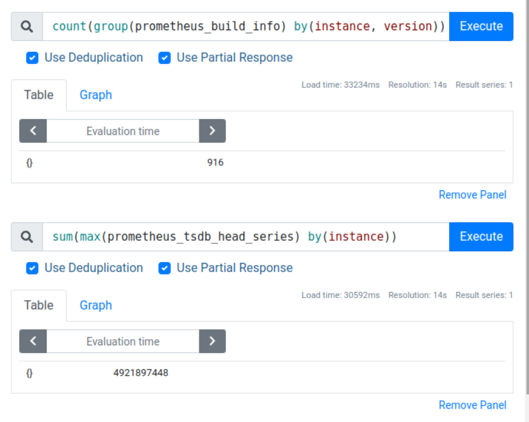
That’s an average of around 5 million time series per instance, but in reality we have a mixture of very tiny and very large instances, with the biggest instances storing around 30 million time series each.
Operating such a large Prometheus deployment doesn’t come without challenges. In this blog post we’ll cover some of the issues one might encounter when trying to collect many millions of time series per Prometheus instance.
Metrics cardinality
One of the first problems you’re likely to hear about when you start running your own Prometheus instances is cardinality, with the most dramatic cases of this problem being referred to as “cardinality explosion”.
So let’s start by looking at what cardinality means from Prometheus’ perspective, when it can be a problem and some of the ways to deal with it.
Let’s say we have an application which we want to instrument, which means add some observable properties in the form of metrics that Prometheus can read from our application. A metric can be anything that you can express as a number, for example:
- The speed at which a vehicle is traveling.
- Current temperature.
- The number of times some specific event occurred.
To create metrics inside our application we can use one of many Prometheus client libraries. Let’s pick client_python for simplicity, but the same concepts will apply regardless of the language you use.
from prometheus_client import Counter

# Declare our first metric.
# First argument is the name of the metric.
# Second argument is the description of it.
c = Counter(mugs_of_beverage_total, 'The total number of mugs drank.')

# Call inc() to increment our metric every time a mug was drank.
c.inc()
c.inc()
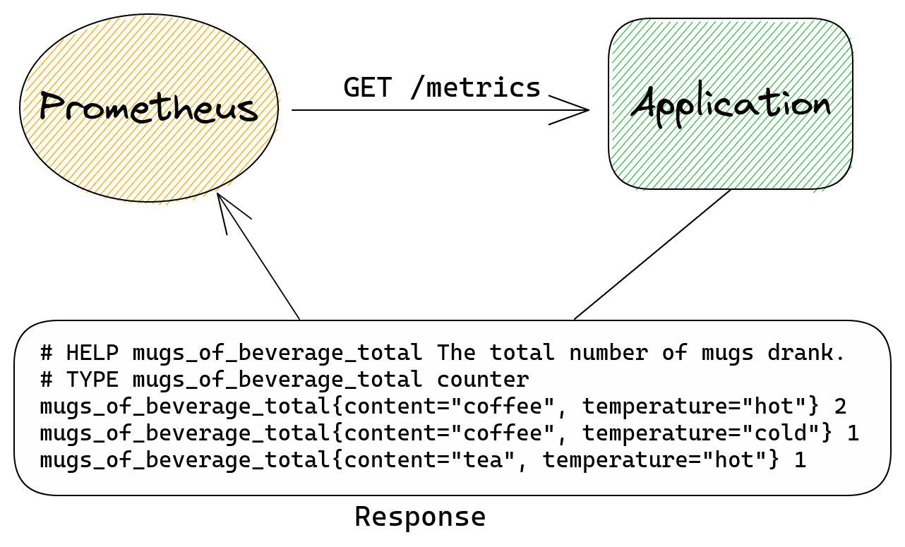
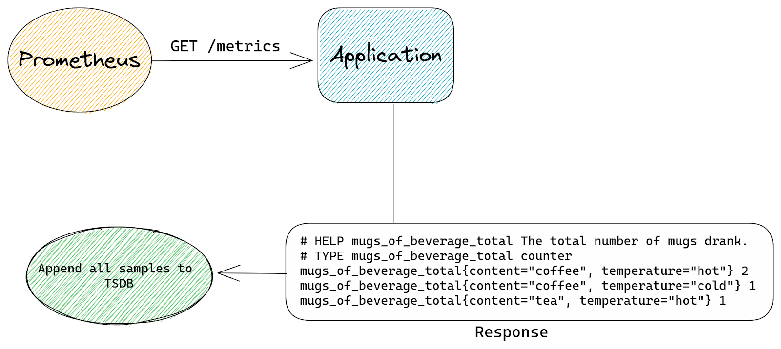
With this simple code Prometheus client library will create a single metric. For Prometheus to collect this metric we need our application to run an HTTP server and expose our metrics there. The simplest way of doing this is by using functionality provided with client_python itself – see documentation here.
When Prometheus sends an HTTP request to our application it will receive this response:
# HELP mugs_of_beverage_total The total number of mugs drank.
# TYPE mugs_of_beverage_total counter
mugs_of_beverage_total 2
This format and underlying data model are both covered extensively in Prometheus’ own documentation.
Please see data model and exposition format pages for more details.
We can add more metrics if we like and they will all appear in the HTTP response to the metrics endpoint.
Prometheus metrics can have extra dimensions in form of labels. We can use these to add more information to our metrics so that we can better understand what’s going on.
With our example metric we know how many mugs were consumed, but what if we also want to know what kind of beverage it was? Or maybe we want to know if it was a cold drink or a hot one? Adding labels is very easy and all we need to do is specify their names. Once we do that we need to pass label values (in the same order as label names were specified) when incrementing our counter to pass this extra information.
Let’s adjust the example code to do this.
from prometheus_client import Counter

c = Counter(mugs_of_beverage_total, 'The total number of mugs drank.', ['content', 'temperature'])

c.labels('coffee', 'hot').inc()
c.labels('coffee', 'hot').inc()
c.labels('coffee', 'cold').inc()
c.labels('tea', 'hot').inc()
Our HTTP response will now show more entries:
# HELP mugs_of_beverage_total The total number of mugs drank.
# TYPE mugs_of_beverage_total counter
mugs_of_beverage_total{content="coffee", temperature="hot"} 2
mugs_of_beverage_total{content="coffee", temperature="cold"} 1
mugs_of_beverage_total{content="tea", temperature="hot"} 1
As we can see we have an entry for each unique combination of labels.
And this brings us to the definition of cardinality in the context of metrics. Cardinality is the number of unique combinations of all labels. The more labels you have and the more values each label can take, the more unique combinations you can create and the higher the cardinality.
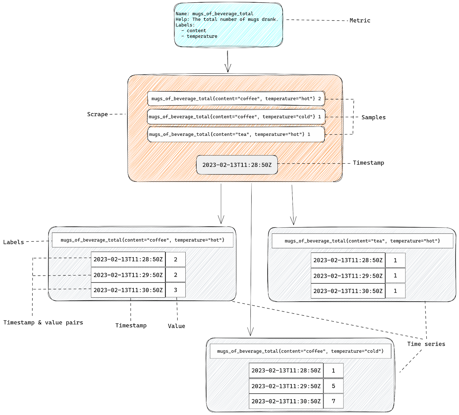
Metrics vs samples vs time series
Now we should pause to make an important distinction between metrics and time series.
A metric is an observable property with some defined dimensions (labels). In our example case it’s a Counter class object.
A time series is an instance of that metric, with a unique combination of all the dimensions (labels), plus a series of timestamp & value pairs – hence the name “time series”. Names and labels tell us what is being observed, while timestamp & value pairs tell us how that observable property changed over time, allowing us to plot graphs using this data.
What this means is that a single metric will create one or more time series. The number of time series depends purely on the number of labels and the number of all possible values these labels can take.
Every time we add a new label to our metric we risk multiplying the number of time series that will be exported to Prometheus as the result.
In our example we have two labels, “content” and “temperature”, and both of them can have two different values. So the maximum number of time series we can end up creating is four (2*2). If we add another label that can also have two values then we can now export up to eight time series (2*2*2). The more labels we have or the more distinct values they can have the more time series as a result.
If all the label values are controlled by your application you will be able to count the number of all possible label combinations. But the real risk is when you create metrics with label values coming from the outside world.
If instead of beverages we tracked the number of HTTP requests to a web server, and we used the request path as one of the label values, then anyone making a huge number of random requests could force our application to create a huge number of time series. To avoid this it’s in general best to never accept label values from untrusted sources.
To make things more complicated you may also hear about “samples” when reading Prometheus documentation. A sample is something in between metric and time series – it’s a time series value for a specific timestamp. Timestamps here can be explicit or implicit. If a sample lacks any explicit timestamp then it means that the sample represents the most recent value – it’s the current value of a given time series, and the timestamp is simply the time you make your observation at.
If you look at the HTTP response of our example metric you’ll see that none of the returned entries have timestamps. There’s no timestamp anywhere actually. This is because the Prometheus server itself is responsible for timestamps. When Prometheus collects metrics it records the time it started each collection and then it will use it to write timestamp & value pairs for each time series.
That’s why what our application exports isn’t really metrics or time series – it’s samples.
Confusing? Let’s recap:
- We start with a metric – that’s simply a definition of something that we can observe, like the number of mugs drunk.
- Our metrics are exposed as a HTTP response. That response will have a list of samples – these are individual instances of our metric (represented by name & labels), plus the current value.
- When Prometheus collects all the samples from our HTTP response it adds the timestamp of that collection and with all this information together we have a time series.
Cardinality related problems
Each time series will cost us resources since it needs to be kept in memory, so the more time series we have, the more resources metrics will consume. This is true both for client libraries and Prometheus server, but it’s more of an issue for Prometheus itself, since a single Prometheus server usually collects metrics from many applications, while an application only keeps its own metrics.
Since we know that the more labels we have the more time series we end up with, you can see when this can become a problem. Simply adding a label with two distinct values to all our metrics might double the number of time series we have to deal with. Which in turn will double the memory usage of our Prometheus server. If we let Prometheus consume more memory than it can physically use then it will crash.
This scenario is often described as “cardinality explosion” – some metric suddenly adds a huge number of distinct label values, creates a huge number of time series, causes Prometheus to run out of memory and you lose all observability as a result.
How is Prometheus using memory?
To better handle problems with cardinality it’s best if we first get a better understanding of how Prometheus works and how time series consume memory.
For that let’s follow all the steps in the life of a time series inside Prometheus.
Step one – HTTP scrape
The process of sending HTTP requests from Prometheus to our application is called “scraping”. Inside the Prometheus configuration file we define a “scrape config” that tells Prometheus where to send the HTTP request, how often and, optionally, to apply extra processing to both requests and responses.
It will record the time it sends HTTP requests and use that later as the timestamp for all collected time series.
After sending a request it will parse the response looking for all the samples exposed there.
Step two – new time series or an update?
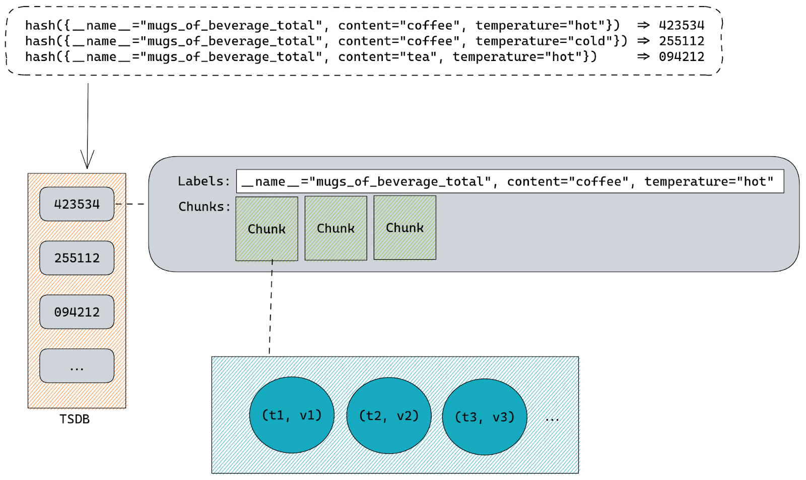
Once Prometheus has a list of samples collected from our application it will save it into TSDB – Time Series DataBase – the database in which Prometheus keeps all the time series.
But before doing that it needs to first check which of the samples belong to the time series that are already present inside TSDB and which are for completely new time series.
As we mentioned before a time series is generated from metrics. There is a single time series for each unique combination of metrics labels.
This means that Prometheus must check if there’s already a time series with identical name and exact same set of labels present. Internally time series names are just another label called __name__, so there is no practical distinction between name and labels. Both of the representations below are different ways of exporting the same time series:
mugs_of_beverage_total{content="tea", temperature="hot"} 1
{__name__="mugs_of_beverage_total", content="tea", temperature="hot"} 1
Since everything is a label Prometheus can simply hash all labels using sha256 or any other algorithm to come up with a single ID that is unique for each time series.
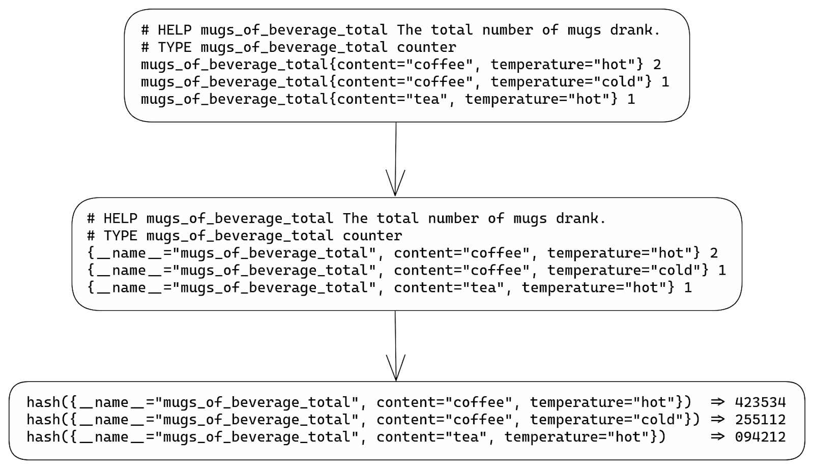
Knowing that it can quickly check if there are any time series already stored inside TSDB that have the same hashed value. Basically our labels hash is used as a primary key inside TSDB.
Step three – appending to TSDB
Once TSDB knows if it has to insert new time series or update existing ones it can start the real work.
Internally all time series are stored inside a map on a structure called Head. That map uses labels hashes as keys and a structure called memSeries as values. Those memSeries objects are storing all the time series information. The struct definition for memSeries is fairly big, but all we really need to know is that it has a copy of all the time series labels and chunks that hold all the samples (timestamp & value pairs).
Labels are stored once per each memSeries instance.
Samples are stored inside chunks using “varbit” encoding which is a lossless compression scheme optimized for time series data. Each chunk represents a series of samples for a specific time range. This helps Prometheus query data faster since all it needs to do is first locate the memSeries instance with labels matching our query and then find the chunks responsible for time range of the query.
By default Prometheus will create a chunk per each two hours of wall clock. So there would be a chunk for: 00:00 – 01:59, 02:00 – 03:59, 04:00 – 05:59, …, 22:00 – 23:59.
There’s only one chunk that we can append to, it’s called the “Head Chunk”. It’s the chunk responsible for the most recent time range, including the time of our scrape. Any other chunk holds historical samples and therefore is read-only.
There is a maximum of 120 samples each chunk can hold. This is because once we have more than 120 samples on a chunk efficiency of “varbit” encoding drops. TSDB will try to estimate when a given chunk will reach 120 samples and it will set the maximum allowed time for current Head Chunk accordingly.
If we try to append a sample with a timestamp higher than the maximum allowed time for current Head Chunk, then TSDB will create a new Head Chunk and calculate a new maximum time for it based on the rate of appends.
All chunks must be aligned to those two hour slots of wall clock time, so if TSDB was building a chunk for 10:00-11:59 and it was already “full” at 11:30 then it would create an extra chunk for the 11:30-11:59 time range.
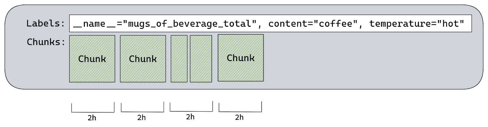
Since the default Prometheus scrape interval is one minute it would take two hours to reach 120 samples.
What this means is that using Prometheus defaults each memSeries should have a single chunk with 120 samples on it for every two hours of data.
Going back to our time series – at this point Prometheus either creates a new memSeries instance or uses already existing memSeries. Once it has a memSeries instance to work with it will append our sample to the Head Chunk. This might require Prometheus to create a new chunk if needed.
Step four – memory-mapping old chunks
After a few hours of Prometheus running and scraping metrics we will likely have more than one chunk on our time series:
- One “Head Chunk” – containing up to two hours of the last two hour wall clock slot.
- One or more for historical ranges – these chunks are only for reading, Prometheus won’t try to append anything here.
Since all these chunks are stored in memory Prometheus will try to reduce memory usage by writing them to disk and memory-mapping. The advantage of doing this is that memory-mapped chunks don’t use memory unless TSDB needs to read them.
The Head Chunk is never memory-mapped, it’s always stored in memory.
Step five – writing blocks to disk
Up until now all time series are stored entirely in memory and the more time series you have, the higher Prometheus memory usage you’ll see. The only exception are memory-mapped chunks which are offloaded to disk, but will be read into memory if needed by queries.
This allows Prometheus to scrape and store thousands of samples per second, our biggest instances are appending 550k samples per second, while also allowing us to query all the metrics simultaneously.
But you can’t keep everything in memory forever, even with memory-mapping parts of data.
Every two hours Prometheus will persist chunks from memory onto the disk. This process is also aligned with the wall clock but shifted by one hour.
When using Prometheus defaults and assuming we have a single chunk for each two hours of wall clock we would see this:
- 02:00 – create a new chunk for 02:00 – 03:59 time range
- 03:00 – write a block for 00:00 – 01:59
- 04:00 – create a new chunk for 04:00 – 05:59 time range
- 05:00 – write a block for 02:00 – 03:59
- …
- 22:00 – create a new chunk for 22:00 – 23:59 time range
- 23:00 – write a block for 20:00 – 21:59
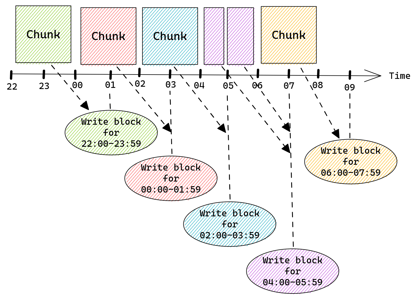
Once a chunk is written into a block it is removed from memSeries and thus from memory. Prometheus will keep each block on disk for the configured retention period.
Blocks will eventually be “compacted”, which means that Prometheus will take multiple blocks and merge them together to form a single block that covers a bigger time range. This process helps to reduce disk usage since each block has an index taking a good chunk of disk space. By merging multiple blocks together, big portions of that index can be reused, allowing Prometheus to store more data using the same amount of storage space.
Step six – garbage collection
After a chunk was written into a block and removed from memSeries we might end up with an instance of memSeries that has no chunks. This would happen if any time series was no longer being exposed by any application and therefore there was no scrape that would try to append more samples to it.
A common pattern is to export software versions as a build_info metric, Prometheus itself does this too:
prometheus_build_info{version="2.42.0"} 1
When Prometheus 2.43.0 is released this metric would be exported as:
prometheus_build_info{version="2.43.0"} 1
Which means that a time series with version=”2.42.0” label would no longer receive any new samples.
Once the last chunk for this time series is written into a block and removed from the memSeries instance we have no chunks left. This means that our memSeries still consumes some memory (mostly labels) but doesn’t really do anything.
To get rid of such time series Prometheus will run “head garbage collection” (remember that Head is the structure holding all memSeries) right after writing a block. This garbage collection, among other things, will look for any time series without a single chunk and remove it from memory.
Since this happens after writing a block, and writing a block happens in the middle of the chunk window (two hour slices aligned to the wall clock) the only memSeries this would find are the ones that are “orphaned” – they received samples before, but not anymore.
What does this all mean?
TSDB used in Prometheus is a special kind of database that was highly optimized for a very specific workload:
- Time series scraped from applications are kept in memory.
- Samples are compressed using encoding that works best if there are continuous updates.
- Chunks that are a few hours old are written to disk and removed from memory.
- When time series disappear from applications and are no longer scraped they still stay in memory until all chunks are written to disk and garbage collection removes them.
This means that Prometheus is most efficient when continuously scraping the same time series over and over again. It’s least efficient when it scrapes a time series just once and never again – doing so comes with a significant memory usage overhead when compared to the amount of information stored using that memory.
If we try to visualize how the perfect type of data Prometheus was designed for looks like we’ll end up with this:
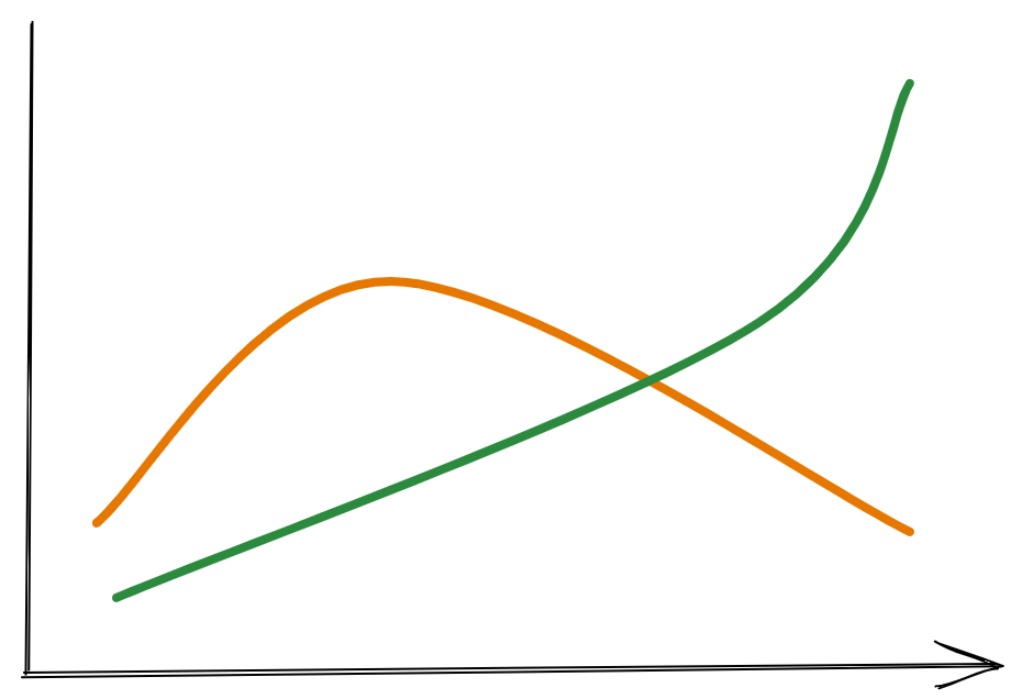
A few continuous lines describing some observed properties.
If, on the other hand, we want to visualize the type of data that Prometheus is the least efficient when dealing with, we’ll end up with this instead:
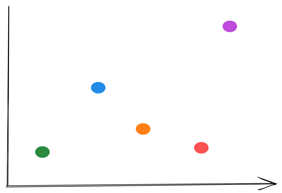
Here we have single data points, each for a different property that we measure.
Although you can tweak some of Prometheus’ behavior and tweak it more for use with short lived time series, by passing one of the hidden flags, it’s generally discouraged to do so. These flags are only exposed for testing and might have a negative impact on other parts of Prometheus server.
To get a better understanding of the impact of a short lived time series on memory usage let’s take a look at another example.
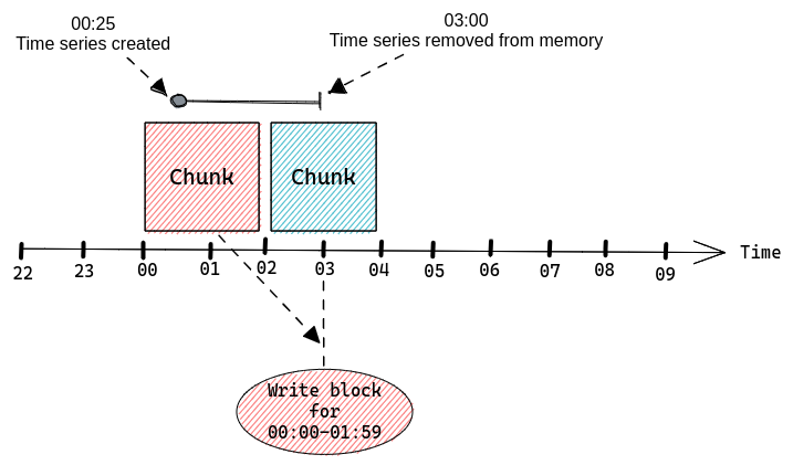
Let’s see what happens if we start our application at 00:25, allow Prometheus to scrape it once while it exports:
prometheus_build_info{version="2.42.0"} 1
And then immediately after the first scrape we upgrade our application to a new version:
prometheus_build_info{version="2.43.0"} 1
At 00:25 Prometheus will create our memSeries, but we will have to wait until Prometheus writes a block that contains data for 00:00-01:59 and runs garbage collection before that memSeries is removed from memory, which will happen at 03:00.
This single sample (data point) will create a time series instance that will stay in memory for over two and a half hours using resources, just so that we have a single timestamp & value pair.
If we were to continuously scrape a lot of time series that only exist for a very brief period then we would be slowly accumulating a lot of memSeries in memory until the next garbage collection.
Looking at memory usage of such Prometheus server we would see this pattern repeating over time:
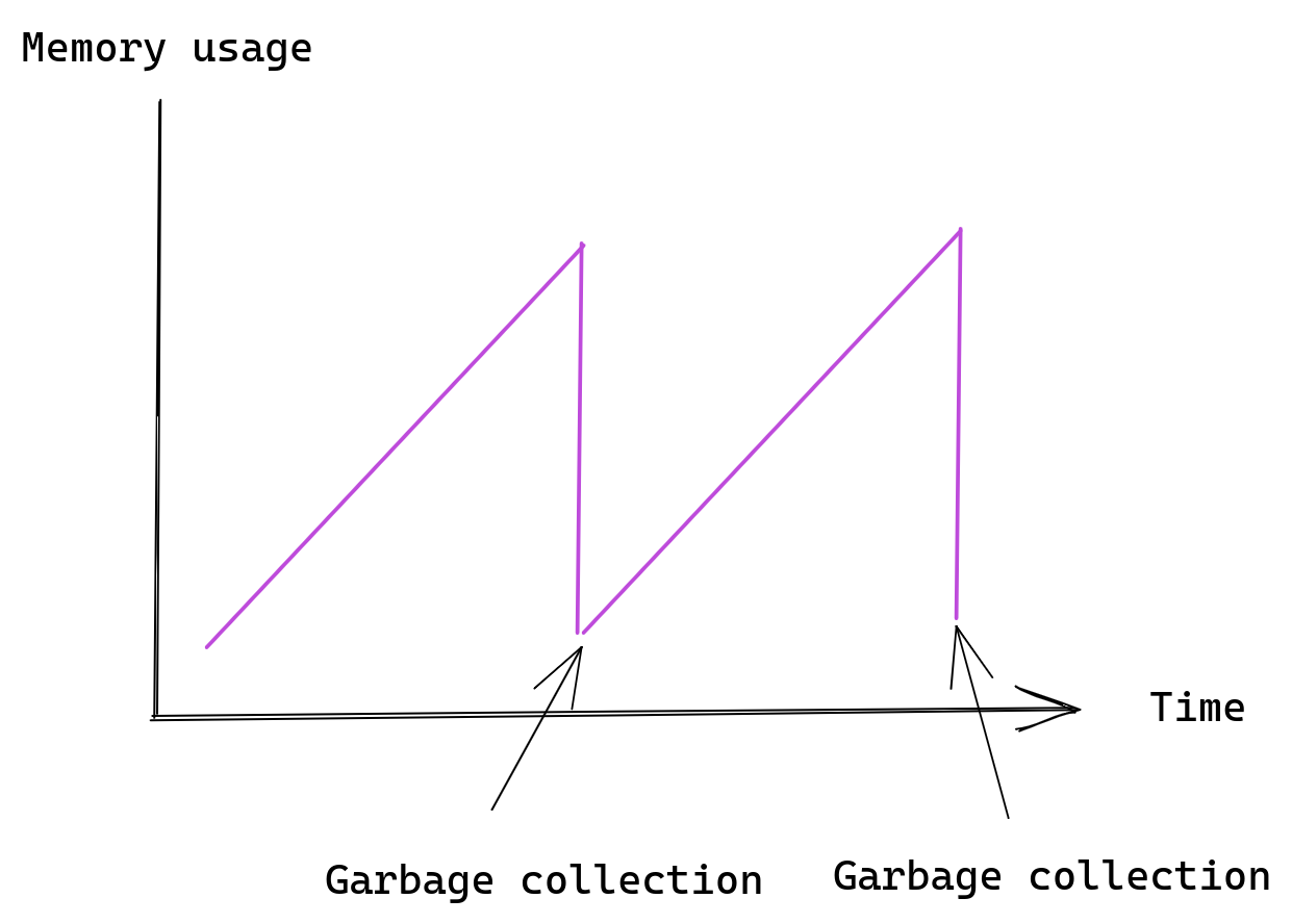
The important information here is that short lived time series are expensive. A time series that was only scraped once is guaranteed to live in Prometheus for one to three hours, depending on the exact time of that scrape.
The cost of cardinality
At this point we should know a few things about Prometheus:
- We know what a metric, a sample and a time series is.
- We know that the more labels on a metric, the more time series it can create.
- We know that each time series will be kept in memory.
- We know that time series will stay in memory for a while, even if they were scraped only once.
With all of that in mind we can now see the problem – a metric with high cardinality, especially one with label values that come from the outside world, can easily create a huge number of time series in a very short time, causing cardinality explosion. This would inflate Prometheus memory usage, which can cause Prometheus server to crash, if it uses all available physical memory.
To get a better idea of this problem let’s adjust our example metric to track HTTP requests.
Our metric will have a single label that stores the request path.
from prometheus_client import Counter

c = Counter(http_requests_total, 'The total number of HTTP requests.', ['path'])

# HTTP request handler our web server will call
def handle_request(path):
  c.labels(path).inc()
  ...
If we make a single request using the curl command:
> curl https://app.example.com/index.html
We should see these time series in our application:
# HELP http_requests_total The total number of HTTP requests.
# TYPE http_requests_total counter
http_requests_total{path="/index.html"} 1
But what happens if an evil hacker decides to send a bunch of random requests to our application?
> curl https://app.example.com/jdfhd5343
> curl https://app.example.com/3434jf833
> curl https://app.example.com/1333ds5
> curl https://app.example.com/aaaa43321
Extra time series would be created:
# HELP http_requests_total The total number of HTTP requests.
# TYPE http_requests_total counter
http_requests_total{path="/index.html"} 1
http_requests_total{path="/jdfhd5343"} 1
http_requests_total{path="/3434jf833"} 1
http_requests_total{path="/1333ds5"} 1
http_requests_total{path="/aaaa43321"} 1
With 1,000 random requests we would end up with 1,000 time series in Prometheus. If our metric had more labels and all of them were set based on the request payload (HTTP method name, IPs, headers, etc) we could easily end up with millions of time series.
Often it doesn’t require any malicious actor to cause cardinality related problems. A common class of mistakes is to have an error label on your metrics and pass raw error objects as values.
from prometheus_client import Counter

c = Counter(errors_total, 'The total number of errors.', [error])

def my_func:
  try:
    ...
  except Exception as err:
    c.labels(err).inc()
This works well if errors that need to be handled are generic, for example “Permission Denied”:
errors_total{error="Permission Denied"} 1
But if the error string contains some task specific information, for example the name of the file that our application didn’t have access to, or a TCP connection error, then we might easily end up with high cardinality metrics this way:
errors_total{error="file not found: /myfile.txt"} 1
errors_total{error="file not found: /other/file.txt"} 1
errors_total{error="read udp 127.0.0.1:12421->127.0.0.2:443: i/o timeout"} 1
errors_total{error="read udp 127.0.0.1:14743->127.0.0.2:443: i/o timeout"} 1
Once scraped all those time series will stay in memory for a minimum of one hour. It’s very easy to keep accumulating time series in Prometheus until you run out of memory.
Even Prometheus’ own client libraries had bugs that could expose you to problems like this.
How much memory does a time series need?
Each time series stored inside Prometheus (as a memSeries instance) consists of:
- Copy of all labels.
- Chunks containing samples.
- Extra fields needed by Prometheus internals.
The amount of memory needed for labels will depend on the number and length of these. The more labels you have, or the longer the names and values are, the more memory it will use.
The way labels are stored internally by Prometheus also matters, but that’s something the user has no control over. There is an open pull request which improves memory usage of labels by storing all labels as a single string.
Chunks will consume more memory as they slowly fill with more samples, after each scrape, and so the memory usage here will follow a cycle – we start with low memory usage when the first sample is appended, then memory usage slowly goes up until a new chunk is created and we start again.
You can calculate how much memory is needed for your time series by running this query on your Prometheus server:
go_memstats_alloc_bytes / prometheus_tsdb_head_series
Note that your Prometheus server must be configured to scrape itself for this to work.
Secondly this calculation is based on all memory used by Prometheus, not only time series data, so it’s just an approximation. Use it to get a rough idea of how much memory is used per time series and don’t assume it’s that exact number.
Thirdly Prometheus is written in Golang which is a language with garbage collection. The actual amount of physical memory needed by Prometheus will usually be higher as a result, since it will include unused (garbage) memory that needs to be freed by Go runtime.
Protecting Prometheus from cardinality explosions
Prometheus does offer some options for dealing with high cardinality problems. There are a number of options you can set in your scrape configuration block. Here is the extract of the relevant options from Prometheus documentation:
# An uncompressed response body larger than this many bytes will cause the
# scrape to fail. 0 means no limit. Example: 100MB.
# This is an experimental feature, this behaviour could
# change or be removed in the future.
[ body_size_limit: <size> | default = 0 ]
# Per-scrape limit on number of scraped samples that will be accepted.
# If more than this number of samples are present after metric relabeling
# the entire scrape will be treated as failed. 0 means no limit.
[ sample_limit: <int> | default = 0 ]

# Per-scrape limit on number of labels that will be accepted for a sample. If
# more than this number of labels are present post metric-relabeling, the
# entire scrape will be treated as failed. 0 means no limit.
[ label_limit: <int> | default = 0 ]

# Per-scrape limit on length of labels name that will be accepted for a sample.
# If a label name is longer than this number post metric-relabeling, the entire
# scrape will be treated as failed. 0 means no limit.
[ label_name_length_limit: <int> | default = 0 ]

# Per-scrape limit on length of labels value that will be accepted for a sample.
# If a label value is longer than this number post metric-relabeling, the
# entire scrape will be treated as failed. 0 means no limit.
[ label_value_length_limit: <int> | default = 0 ]

# Per-scrape config limit on number of unique targets that will be
# accepted. If more than this number of targets are present after target
# relabeling, Prometheus will mark the targets as failed without scraping them.
# 0 means no limit. This is an experimental feature, this behaviour could
# change in the future.
[ target_limit: <int> | default = 0 ]
Setting all the label length related limits allows you to avoid a situation where extremely long label names or values end up taking too much memory.
Going back to our metric with error labels we could imagine a scenario where some operation returns a huge error message, or even stack trace with hundreds of lines. If such a stack trace ended up as a label value it would take a lot more memory than other time series, potentially even megabytes. Since labels are copied around when Prometheus is handling queries this could cause significant memory usage increase.
Setting label_limit provides some cardinality protection, but even with just one label name and huge number of values we can see high cardinality. Passing sample_limit is the ultimate protection from high cardinality. It enables us to enforce a hard limit on the number of time series we can scrape from each application instance.
The downside of all these limits is that breaching any of them will cause an error for the entire scrape.
If we configure a sample_limit of 100 and our metrics response contains 101 samples, then Prometheus won’t scrape anything at all. This is a deliberate design decision made by Prometheus developers.
The main motivation seems to be that dealing with partially scraped metrics is difficult and you’re better off treating failed scrapes as incidents.
How does Cloudflare deal with high cardinality?
We have hundreds of data centers spread across the world, each with dedicated Prometheus servers responsible for scraping all metrics.
Each Prometheus is scraping a few hundred different applications, each running on a few hundred servers.
Combined that’s a lot of different metrics. It’s not difficult to accidentally cause cardinality problems and in the past we’ve dealt with a fair number of issues relating to it.
Basic limits
The most basic layer of protection that we deploy are scrape limits, which we enforce on all configured scrapes. These are the sane defaults that 99% of application exporting metrics would never exceed.
By default we allow up to 64 labels on each time series, which is way more than most metrics would use.
We also limit the length of label names and values to 128 and 512 characters, which again is more than enough for the vast majority of scrapes.
Finally we do, by default, set sample_limit to 200 – so each application can export up to 200 time series without any action.
What happens when somebody wants to export more time series or use longer labels? All they have to do is set it explicitly in their scrape configuration.
Those limits are there to catch accidents and also to make sure that if any application is exporting a high number of time series (more than 200) the team responsible for it knows about it. This helps us avoid a situation where applications are exporting thousands of times series that aren’t really needed. Once you cross the 200 time series mark, you should start thinking about your metrics more.
CI validation
The next layer of protection is checks that run in CI (Continuous Integration) when someone makes a pull request to add new or modify existing scrape configuration for their application.
These checks are designed to ensure that we have enough capacity on all Prometheus servers to accommodate extra time series, if that change would result in extra time series being collected.
For example, if someone wants to modify sample_limit, let’s say by changing existing limit of 500 to 2,000, for a scrape with 10 targets, that’s an increase of 1,500 per target, with 10 targets that’s 10*1,500=15,000 extra time series that might be scraped. Our CI would check that all Prometheus servers have spare capacity for at least 15,000 time series before the pull request is allowed to be merged.
This gives us confidence that we won’t overload any Prometheus server after applying changes.
Our custom patches
One of the most important layers of protection is a set of patches we maintain on top of Prometheus. There is an open pull request on the Prometheus repository. This patchset consists of two main elements.
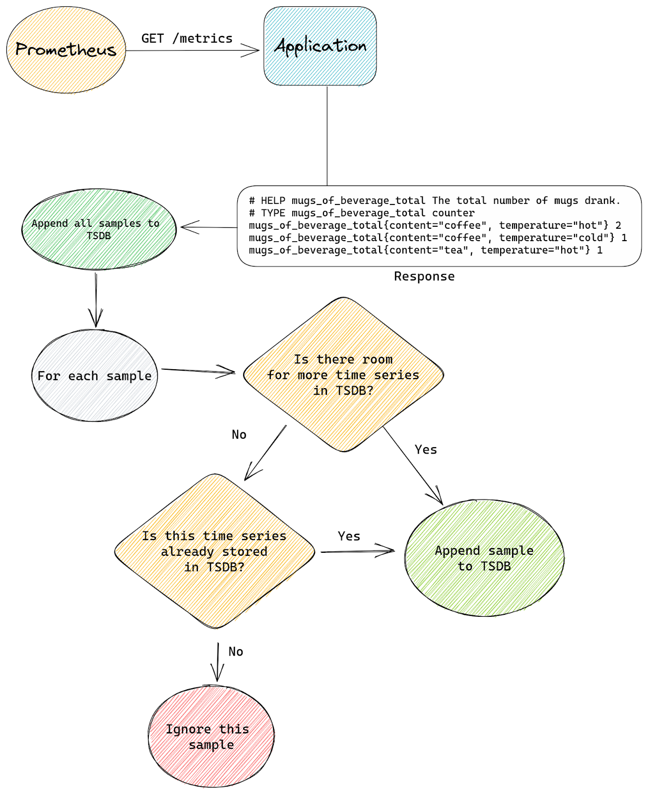
First is the patch that allows us to enforce a limit on the total number of time series TSDB can store at any time. There is no equivalent functionality in a standard build of Prometheus, if any scrape produces some samples they will be appended to time series inside TSDB, creating new time series if needed.
This is the standard flow with a scrape that doesn’t set any sample_limit:
With our patch we tell TSDB that it’s allowed to store up to N time series in total, from all scrapes, at any time. So when TSDB is asked to append a new sample by any scrape, it will first check how many time series are already present.
If the total number of stored time series is below the configured limit then we append the sample as usual.
The difference with standard Prometheus starts when a new sample is about to be appended, but TSDB already stores the maximum number of time series it’s allowed to have. Our patched logic will then check if the sample we’re about to append belongs to a time series that’s already stored inside TSDB or is it a new time series that needs to be created.
If the time series already exists inside TSDB then we allow the append to continue. If the time series doesn’t exist yet and our append would create it (a new memSeries instance would be created) then we skip this sample. We will also signal back to the scrape logic that some samples were skipped.
This is the modified flow with our patch:
By running “go_memstats_alloc_bytes / prometheus_tsdb_head_series” query we know how much memory we need per single time series (on average), we also know how much physical memory we have available for Prometheus on each server, which means that we can easily calculate the rough number of time series we can store inside Prometheus, taking into account the fact the there’s garbage collection overhead since Prometheus is written in Go:
memory available to Prometheus / bytes per time series = our capacity
This doesn’t capture all complexities of Prometheus but gives us a rough estimate of how many time series we can expect to have capacity for.
By setting this limit on all our Prometheus servers we know that it will never scrape more time series than we have memory for. This is the last line of defense for us that avoids the risk of the Prometheus server crashing due to lack of memory.
The second patch modifies how Prometheus handles sample_limit – with our patch instead of failing the entire scrape it simply ignores excess time series. If we have a scrape with sample_limit set to 200 and the application exposes 201 time series, then all except one final time series will be accepted.
This is the standard Prometheus flow for a scrape that has the sample_limit option set:
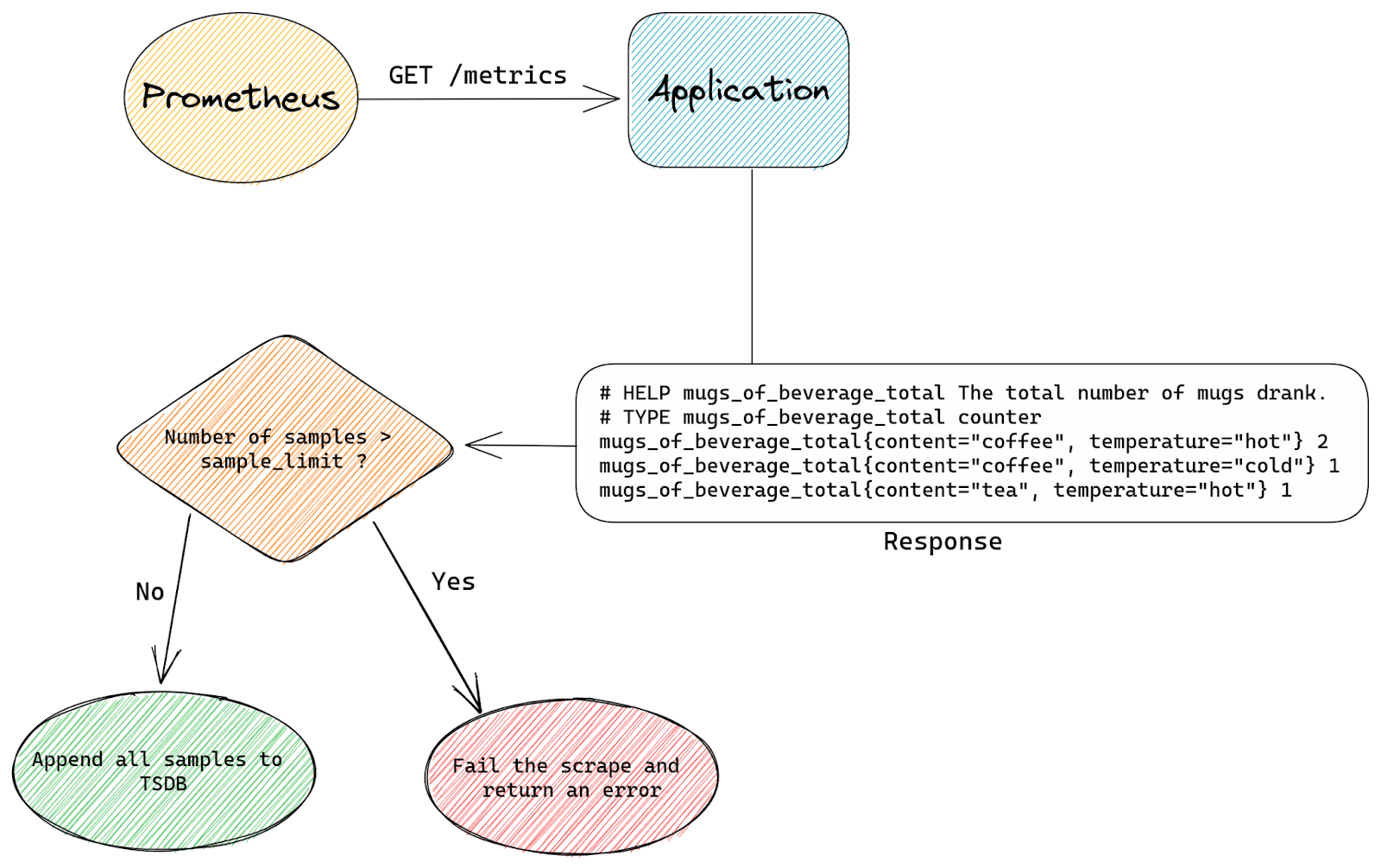
The entire scrape either succeeds or fails. Prometheus simply counts how many samples are there in a scrape and if that’s more than sample_limit allows it will fail the scrape.
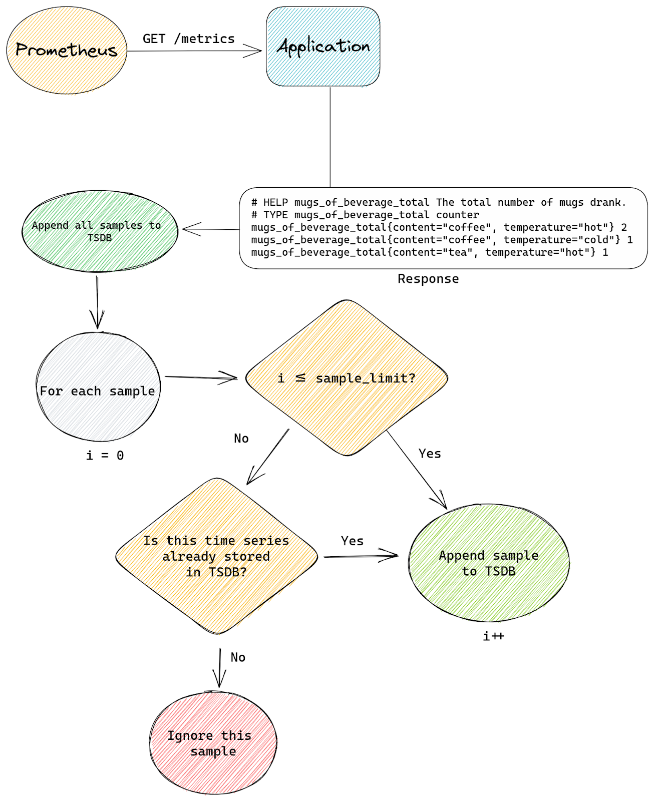
With our custom patch we don’t care how many samples are in a scrape. Instead we count time series as we append them to TSDB. Once we appended sample_limit number of samples we start to be selective.
Any excess samples (after reaching sample_limit) will only be appended if they belong to time series that are already stored inside TSDB.
The reason why we still allow appends for some samples even after we’re above sample_limit is that appending samples to existing time series is cheap, it’s just adding an extra timestamp & value pair.
Creating new time series on the other hand is a lot more expensive – we need to allocate new memSeries instances with a copy of all labels and keep it in memory for at least an hour.
This is how our modified flow looks:
Both patches give us two levels of protection.
The TSDB limit patch protects the entire Prometheus from being overloaded by too many time series.
This is because the only way to stop time series from eating memory is to prevent them from being appended to TSDB. Once they’re in TSDB it’s already too late.
While the sample_limit patch stops individual scrapes from using too much Prometheus capacity, which could lead to creating too many time series in total and exhausting total Prometheus capacity (enforced by the first patch), which would in turn affect all other scrapes since some new time series would have to be ignored. At the same time our patch gives us graceful degradation by capping time series from each scrape to a certain level, rather than failing hard and dropping all time series from affected scrape, which would mean losing all observability of affected applications.
It’s also worth mentioning that without our TSDB total limit patch we could keep adding new scrapes to Prometheus and that alone could lead to exhausting all available capacity, even if each scrape had sample_limit set and scraped fewer time series than this limit allows.
Extra metrics exported by Prometheus itself tell us if any scrape is exceeding the limit and if that happens we alert the team responsible for it.
This also has the benefit of allowing us to self-serve capacity management – there’s no need for a team that signs off on your allocations, if CI checks are passing then we have the capacity you need for your applications.
The main reason why we prefer graceful degradation is that we want our engineers to be able to deploy applications and their metrics with confidence without being subject matter experts in Prometheus. That way even the most inexperienced engineers can start exporting metrics without constantly wondering “Will this cause an incident?”.
Another reason is that trying to stay on top of your usage can be a challenging task. It might seem simple on the surface, after all you just need to stop yourself from creating too many metrics, adding too many labels or setting label values from untrusted sources.
In reality though this is as simple as trying to ensure your application doesn’t use too many resources, like CPU or memory – you can achieve this by simply allocating less memory and doing fewer computations. It doesn’t get easier than that, until you actually try to do it. The more any application does for you, the more useful it is, the more resources it might need. Your needs or your customers’ needs will evolve over time and so you can’t just draw a line on how many bytes or cpu cycles it can consume. If you do that, the line will eventually be redrawn, many times over.
In general, having more labels on your metrics allows you to gain more insight, and so the more complicated the application you’re trying to monitor, the more need for extra labels.
In addition to that in most cases we don’t see all possible label values at the same time, it’s usually a small subset of all possible combinations. For example our errors_total metric, which we used in example before, might not be present at all until we start seeing some errors, and even then it might be just one or two errors that will be recorded. This holds true for a lot of labels that we see are being used by engineers.
This means that looking at how many time series an application could potentially export, and how many it actually exports, gives us two completely different numbers, which makes capacity planning a lot harder.
Especially when dealing with big applications maintained in part by multiple different teams, each exporting some metrics from their part of the stack.
For that reason we do tolerate some percentage of short lived time series even if they are not a perfect fit for Prometheus and cost us more memory.
Documentation
Finally we maintain a set of internal documentation pages that try to guide engineers through the process of scraping and working with metrics, with a lot of information that’s specific to our environment.
Prometheus and PromQL (Prometheus Query Language) are conceptually very simple, but this means that all the complexity is hidden in the interactions between different elements of the whole metrics pipeline.
Managing the entire lifecycle of a metric from an engineering perspective is a complex process.
You must define your metrics in your application, with names and labels that will allow you to work with resulting time series easily. Then you must configure Prometheus scrapes in the correct way and deploy that to the right Prometheus server. Next you will likely need to create recording and/or alerting rules to make use of your time series. Finally you will want to create a dashboard to visualize all your metrics and be able to spot trends.
There will be traps and room for mistakes at all stages of this process. We covered some of the most basic pitfalls in our previous blog post on Prometheus – Monitoring our monitoring. In the same blog post we also mention one of the tools we use to help our engineers write valid Prometheus alerting rules.
Having good internal documentation that covers all of the basics specific for our environment and most common tasks is very important. Being able to answer “How do I X?” yourself without having to wait for a subject matter expert allows everyone to be more productive and move faster, while also avoiding Prometheus experts from answering the same questions over and over again.
Closing thoughts
Prometheus is a great and reliable tool, but dealing with high cardinality issues, especially in an environment where a lot of different applications are scraped by the same Prometheus server, can be challenging.
We had a fair share of problems with overloaded Prometheus instances in the past and developed a number of tools that help us deal with them, including custom patches.
But the key to tackling high cardinality was better understanding how Prometheus works and what kind of usage patterns will be problematic.
Having better insight into Prometheus internals allows us to maintain a fast and reliable observability platform without too much red tape, and the tooling we’ve developed around it, some of which is open sourced, helps our engineers avoid most common pitfalls and deploy with confidence.
How to send web push notifications using Amazon Pinpoint
Post Syndicated from arrohan original https://aws.amazon.com/blogs/messaging-and-targeting/how-to-send-web-push-notifications-using-amazon-pinpoint/
How to send push notifications on any website using AWS messaging tools
Web Push Notifications (also known as browser push notifications) are messages from a website you receive in your browser. These messages are intended to be rich, contextual, timely, personalized and best used to engage, re-engage, and retain website visitors. For instance, as a website owner you could use web push notifications to notify users about sales, important updates or new content on your website.
How are web push notifications different from native app push notifications?
Push notifications are short messages that are displayed directly on the user’s screen sent via mobile applications, providing timely information and messages like order status, promotions, or relevant news in the application.
Web push notifications are simply push notifications sent via web browsers (the browser application on the device), and they work across platforms – Desktop, mobile and tablet. They are a newer channel than push notifications, and have now become a part of the modern marketing strategy alongside native app push notifications, emails and SMS.
In the case of mobile apps, the user must install the application to receive push notifications. In the case of web push, there is no need to download any software—it just takes one click on your website.
Why are Web Push Notifications useful?
Let’s consider a real-world example. Suppose you are an e-commerce website where customers can purchase products. Once, the purchase has been made, customers would be interested in getting real time updates of where the package is in transit, when is it likely to be delivered, a confirmation that the shipment has been delivered and so on. Web push notifications can be an excellent way of providing such updates. Accessing email on mobile devices is often unwieldy, SMS messages cannot support images and are constrained in length (also they typically they cost more money to send!). Push notifications are perfect for such a use case. Till now, the major constraint was that it would require users to install your app on their device. Web push notifications gives website owners and customers the power of push notifications without any need for driving app installs.
Marketers in a variety of sectors like travel, publishing, restaurant & delivery, finance and insurance can use push notifications to improve their down-to-funnel conversions. From new content alerts to limited-time promotions to upcoming events, push messages are short, crisp and drive engagement, conversion, and retention. A short search on the AWS blogs website gives us a number of examples of businesses who have created value for their customers with the help of push notifications. Some of the key advantages of web push notifications are:
- Easy opt in model: Unlike other marketing channels like email or SMS, web push notifications offer users a seamless opt-in experience ― Users simply select `Allow’ on a browser permission prompt. Users do not have to worry about sharing their personal data, like their name, email, or phone number nor do they have to go to the play store/app store and install an app on their device.
- Increased Engagement: Push notifications appear on a user’s desktop or mobile screen and are quick to grab attention. Since push messages are real time and have high visibility – they typically enjoy higher “Click Through Rate (CTR)” as compared to other channels like SMS or email.
- Reach users even when they are not on your website: Web Push Notifications from your website are delivered and shown to the customer even if the user is visiting some other site or on some other app. In this respect (and most others), it is quite similar to app push notifications. Even if subscribers were offline when you sent your push campaign, they will get the push message delivered to them the next time they come online.
- No need for users to install native apps: One of the most compelling reason for installing mobile apps, is because users could stay updated with the latest and the greatest – thanks to app push notifications. The additional cost of going to the play store/app store and installing the app is something which would often discourage users. This is especially true for countries and regions where users are still on lower end phones with limited storage space. Users would often have to uninstall apps (which might include yours too) that they do not use frequently in order to make space for other stuff.
- Makes websites richer and more memorable: If you ask a room of developers what mobile device features are missing from the web, push notifications are always high on the list. This is no longer the case since browsers are increasingly adding support for web push notifications and this has offered website owners a powerful cross platform (Desktop & Mobile, Android & iOS) alternative as against developing and maintaining different native apps for different platforms. Web push notifications even appear quite similar to native mobile push on most smartphones.
- Lower Cost: Unlike channels like SMS, sending web push notifications is absolutely free as browsers themselves offer support for it by adhering to the web push protocol. The only costs incurred will be that of sending push notifications as per the Pinpoint pricing policy.
- Popular browsers support web push: Google Chrome, Firefox, Opera, Edge support web push on both Mobile and Desktop. What’s more the support for web push is continuously getting better. Refer to this link for the latest support status matrix across browsers and form factors.
What is Amazon Pinpoint?
Amazon Pinpoint is an AWS service that provides scalable, targeted multichannel communications. Amazon Pinpoint enables companies to send messages to customers through SMS, push notifications, in-app notifications, email, and voice channels. To learn more about Amazon Pinpoint, visit the website and documentation.
Web Push support on Firebase Cloud Messaging (FCM):
Firebase uses cloud services for its notification services on Android, iOS & Web. Firebase Cloud Messaging or FCM run on basic principles of tokens, which is uniquely generated for each device & later used for sending messages to respective devices. There are two key advantages of using FCM for sending web push notifications:
- Abstracts away the complexity of onboarding to the web push protocol for push messages: Sending web push notifications directly without any third party in between requires your website to add support for the web push protocol. Adherence to the web push protocol requires website owners to perform some steps specific to wpn like adding VAPID headers and payload encryption of push messages. This would be additional work for website owners, especially for those businesses which are already onboarded to FCM for sending native app push notifications. FCM server side apis for sending web push notifications work pretty much the same way as they work for native apps. They abstract away the additional complexity of sending web push messages.
- Send push notifications from Amazon Pinpoint via FCM: Amazon Pinpoint already supports integration with FCM, refer to documentation. Similar to how we add a FCM project in Pinpoint to send push messages to native android apps, in this blog post we will see how a similar integration can be leveraged to send web push notifications.
Advantages of sending Web Push Notifications with Amazon Pinpoint:
Now at this point, you might be thinking, Web push notifications can go a long way towards delighting customers and FCM already abstracts the complexities of sending web push. So why do I need Amazon Pinpoint?
Well, integration with Amazon Pinpoint offers a number of advantages. Here are a few:
- Map FCM tokens to actual users and web app ‘installs’: FCM would give you tokens for each user on your website who subscribes for web push. Roughly speaking, an FCM token for each web app install with permissions to send push messages. To be able to send messages to these users we would need to store the FCM tokens for each user/web app install/browser instance. Amazon Pinpoint treats each browser instance as an endpoint and enables you to save the push tokens in the same way in which we would store native push tokens/mobile numbers/email addresses, i.e., as a primary identifier for that endpoint. This enables us to send messages to Pinpoint endpoints without caring about the underlying complexity of storing and managing push tokens.
- Intelligently send web push, map user attributes to push tokens: Along with the push token, each pinpoint endpoint can also store other attributes like device characteristics, user Id and user attributes. This helps us to create dynamic and complex segments which can be used to send targeted web push notifications.
- It is essentially the same as sending android native push: Create an FCM project, create FCM tokens, Create Pinpoint endpoints with the tokens, send push campaigns to those endpoints. Swap out native android code with service workers, JavaScript on the client and you get web push. It really is that simple.
- Web push, native push, SMS or emails. One stop shop for reaching out to users on all channels: Pinpoint becomes your single backend for reaching out to users across multiple channels. For app users, send them app push, for users who prefer the web, you have web push.
- Leverage Pinpoint features like Campaign Management, Events, Analytics and Segments: Read up about Amazon Pinpoint. It has a lot of great features which can help you better engage your users.
In this blog we will see how to send web push notifications using Amazon Pinpoint on a website built using AWS Amplify.
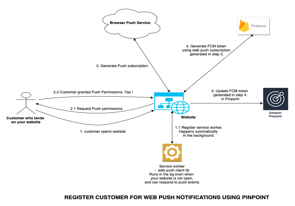
Overview of solution
Enable web push by using FCM as an intermediary service and Pinpoint as an app server (map FCM tokens to actual users) and a push campaign management tool. Integrate web push protocol, FCM and Amazon Pinpoint.
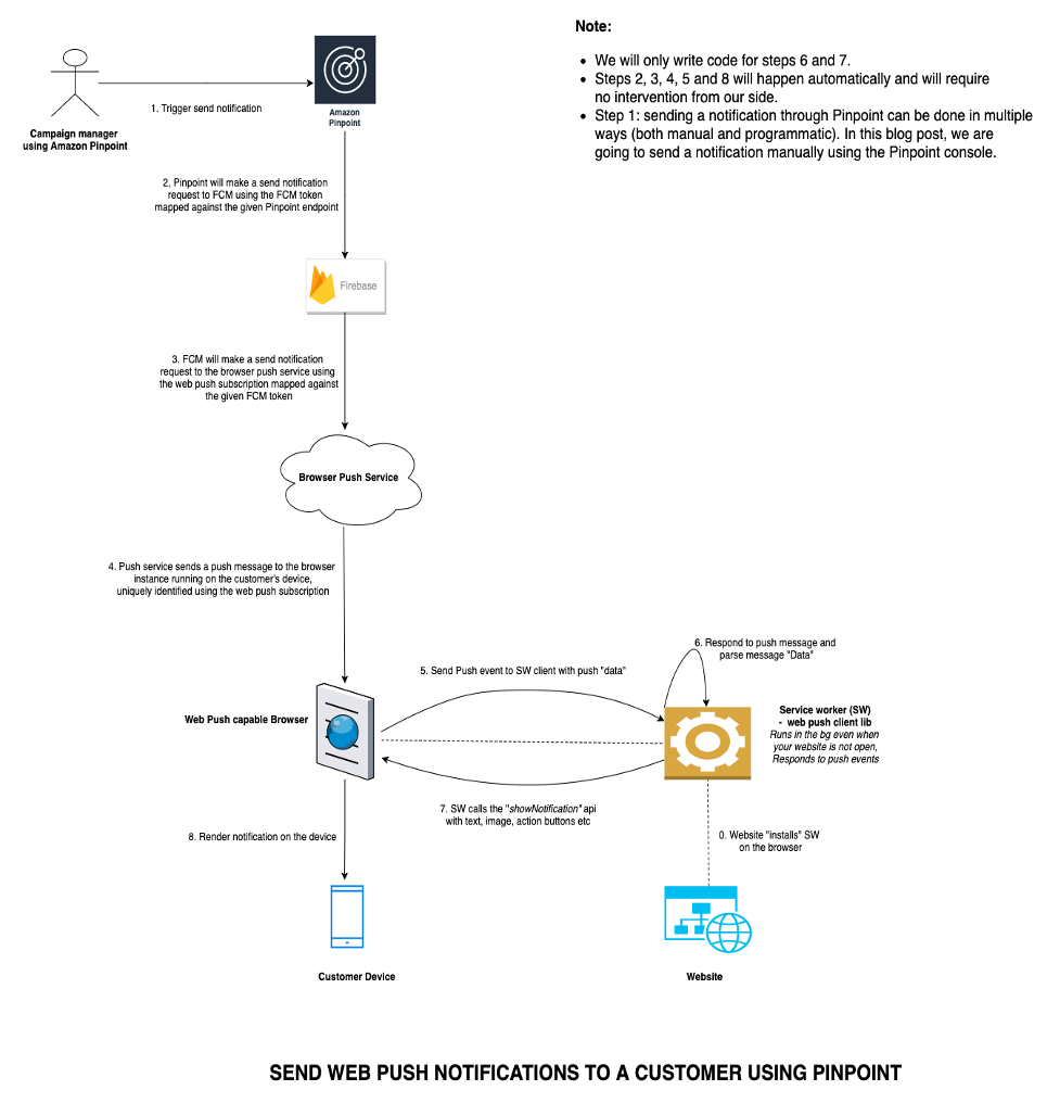
Walkthrough
In this blog post, we will create a simple demo website using Amplify which can be used to create web push subscriptions and also receive web push messages. We will integrate this website with FCM js sdk and Amazon Pinpoint to store the FCM push tokens on Pinpoint. Later we will see how to send web push notifications using Amazon Pinpoint with FCM acting as an intermediary.
The above can be broken down into the below simple and independent steps:
- Create a project on FCM.
- Generate web push notifications server keys on FCM.
- Create a simple web app (website) using Amplify
- Create an Amazon Pinpoint project. This is a one-line command which will be done as part of Amplify web app setup.
- Make your amplify website web push capable. In this step we will also integrate with the FCM sdk for web push.
- Configure the Pinpoint project and integrate it with FCM. It just involves adding the FCM server key to Pinpoint.
- Go to the Amazon Pinpoint console and send a test web push message from your website. And we are done!
You can see checkout my demo website here.
The source code for this demo website (and the blog) is available here.
Prerequisites – Essentials
For this walkthrough, you should have the following prerequisites:
- An AWS account and a FCM developer account.
- Create a FCM project on the Firebase Developer Console. You need to have a FCM developer account to access the console.
- Node and npm.
- AWS Amplify cli setup
- A browser which supports web push notifications and the web push protocol. Refer Browser support matrix.
Prerequisites – Recommended
In addition to the necessary prerequisites mentioned above, I would highly recommend readers to go through the below in order to derive maximum value from this blog post.
- Web Push fundamentals: Some basic reading up on web push notifications and going through a couple of relevant code samples. It is not compulsory to implement and understand everything, but it would be beneficial to have an elementary understanding of service workers, permissions, push subscriptions and notifications apis.
- Introduction: Some of the sections are a bit detailed and complex, you need not go through all the sections completely at once. However, at least go through the overview and the how push works sections carefully.
- Simple Code demo with explanations to help you get started.
- FCM client-side code : You need not go through the send Message sections since we will not directly use FCM apis or the console. Instead, we will use the Pinpoint console to manage our push campaigns.
- Building web apps with amplify: By the end of the tutorial, you should get clarity on how to build and host web apps using amplify. It will also help you become familiar with the amplify cli tool.
- Read up on Amazon Pinpoint.
Setting up the demo web app
Let’s deploy the demo web app using AWS Amplify to see how all the parts come together.
Clone the code for the sample web app
git clone ssh://git.amazon.com/pkg/ArrohanWebPushPoc (branch: PinpointBlog) <github_link>
Create an FCM account and a project on the FCM developer console, on the FCM project add web push as a channel
It is possible that Firebase may change the UI of the console in the future so the given screenshots may not be exactly reflective of the UI, but the broad steps would remain the same.
- Under “Engage” click on ‘Cloud Messaging Tab’. The page url should typically be of the form: https://console.firebase.google.com/u/0/project/<name_of_your_project>/notification.
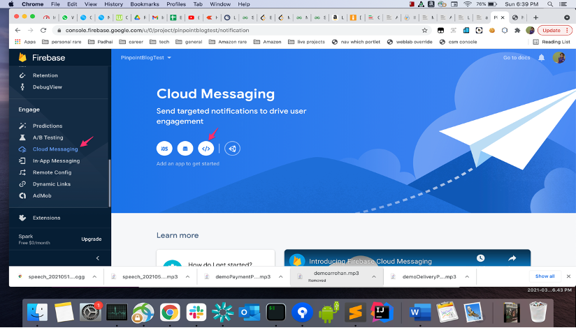
- Under the option “Add an app to get started”, Click on the “web/javascript” (the one with the </> symbol) app.
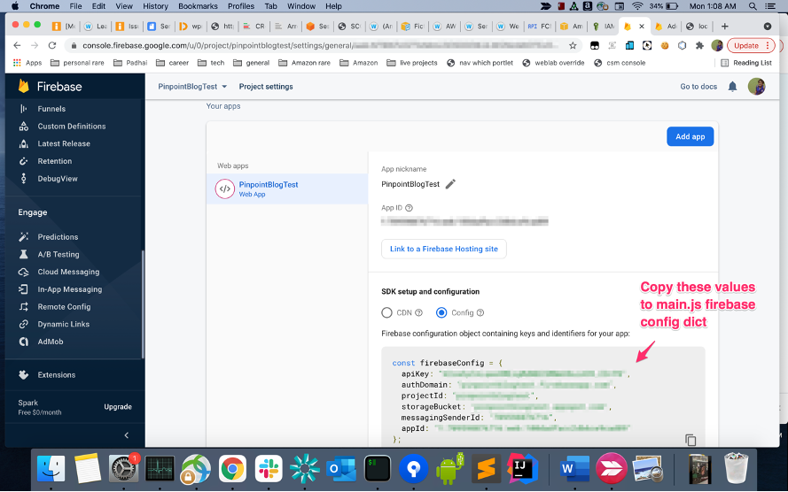
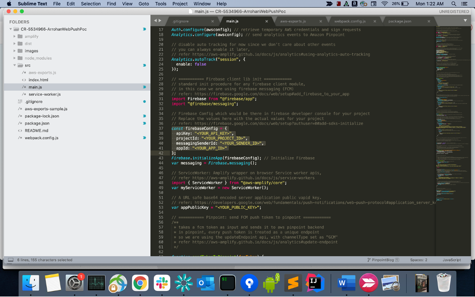
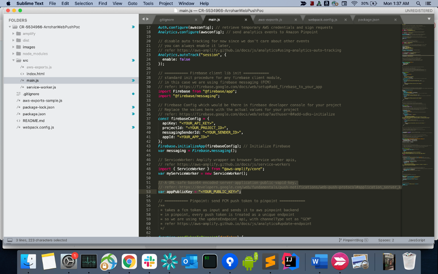
- Once you have created the project, go to project settings. Click on General Tab. Replace the values in
firebaseConfig main.jswith the actual values for your project.
Generate a public-private key pair for the FCM cloud messaging project
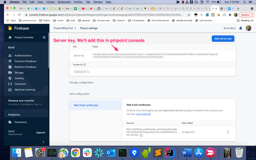
- Under project settings, switch to the cloud messaging tab. Click generate key pair under web push certificates to generate a public-private key pair.
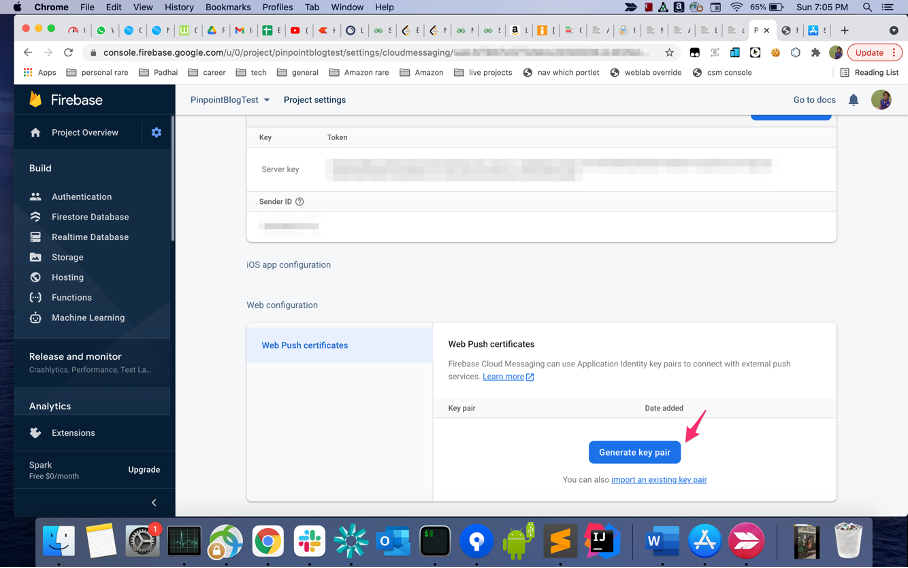
- Replace the
<YOUR PUBLIC KEY>in the filemain.jsin the source code with the vapid public key you generated in the previous step.
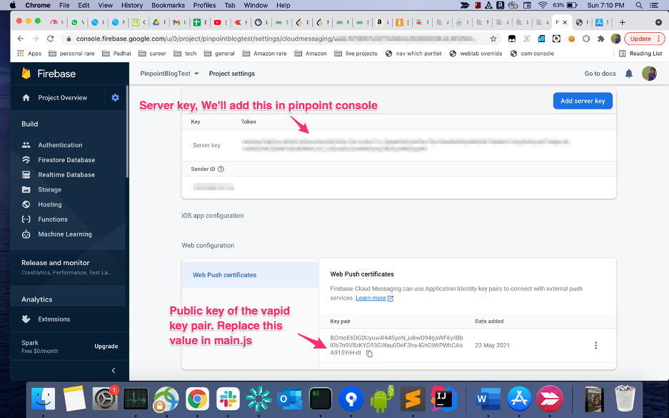
- Note the Server key, you will need it during pinpoint project setup.
Setup an Amplify web app and integrate with pinpoint
- Clone the code in the given repo, replace your FCM config and keys. Run
npm install.- In case you face build errors due to package versions getting outdated (firebase, especially gets updated often, sometimes with breaking changes), please update the dependencies to the latest version. This post offers an easy way to identify outdated dependencies and update them.
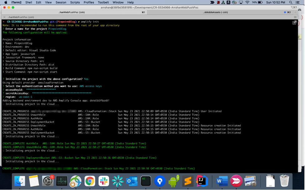
- Setup an Amplify web app. Note, for the purpose of this demo, you just need to setup a simple static website. Simply run
amplify init. Enter the required details, the default config should work fine.
- Create a pinpoint project and integrate with our web app through amplify cli:
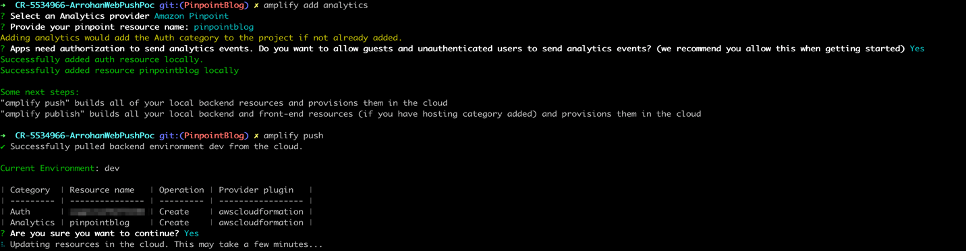
- Create a pinpoint project: Run
amplify add analytics. ChooseAmazon Pinpointas the analytics provider and accept all defaults. - Please note when you add “analytics” to the project you will get a prompt which says something like – “Apps need authorization to send analytics events. Do you want to allow guests and unauthenticated users to send analytics events? (We recommend you allow this when getting started)” – Please accept and answer
Yeswhen you get this. - Push to AWS: Run
amplify push. A configuration file (aws-exports.js) will be added to the source directory. Notice, we are calling this file from our main.js file.
- Create a pinpoint project: Run
Pinpoint Project setup
- Get the Server key of the FCM project you created earlier.
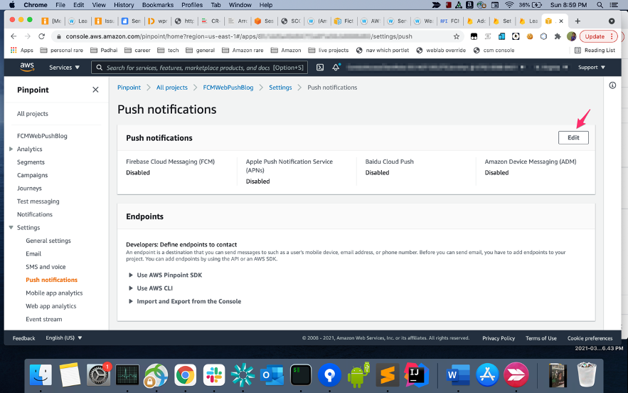
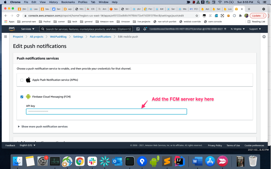
- Open the pinpoint project you created in the previous step on the Pinpoint console. Add FCM Legacy server key to the Project. The process is exactly the same as one would follow for native android apps.
Run the web app and subscribe for push notifications
- Run
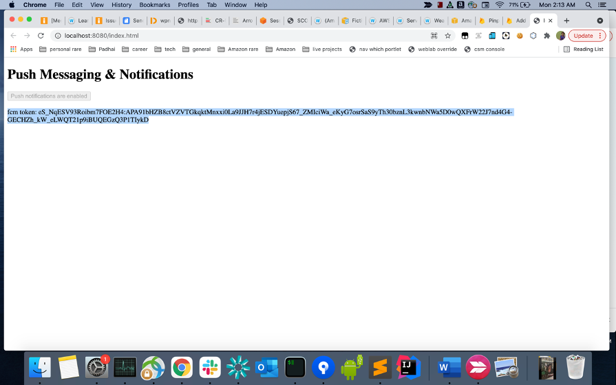
npm start, our web app will be running on http://localhost:8080/index.html - Click on enable push messages and click allow/accept on the browser permission prompt which follows. Once it is enabled, you will see a FCM token on the page, copy the token.
Send a web push notification from the Amazon Pinpoint console
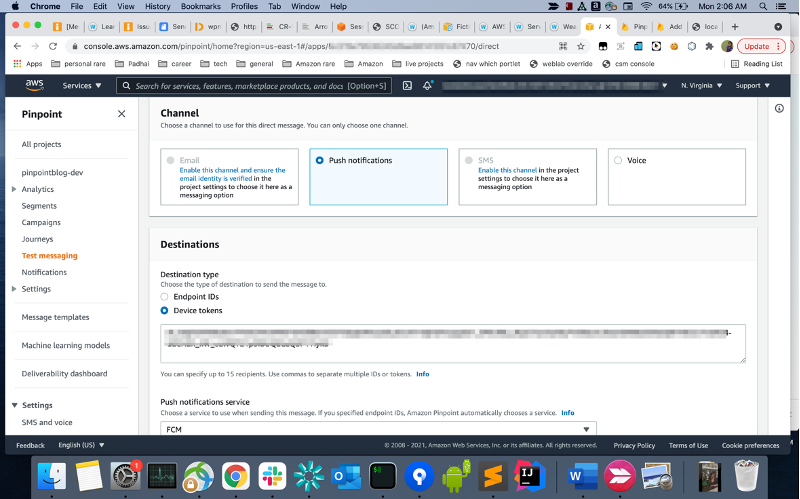
- Open the pinpoint project you created in the previous step on the Pinpoint console. Click on your project and then go to test messaging. The process is exactly the same as the one for native apps described here. Under “destination type” select “Device Tokens” and paste the FCM token you copied in the previous step.
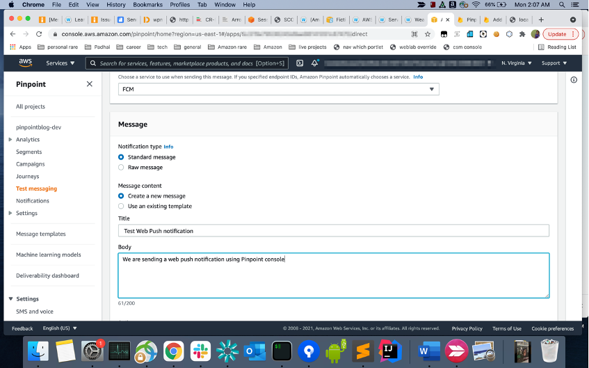
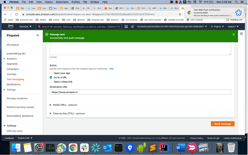
- Fill in title, body and optionally URL (“Go to a URL” under “Actions”). Click on Send Message, you should get a push message on your browser.
Next steps
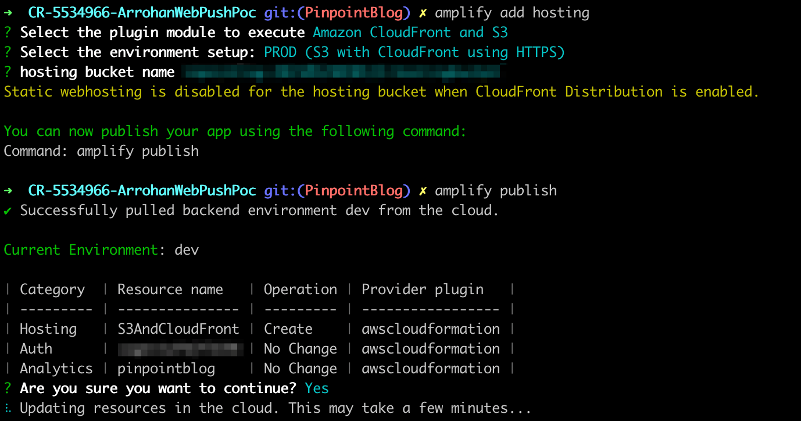
- Host your app. Simply run
amplify add hostingfollowed byamplify publish. Remember that for web push (service workers) to work, your site should be https.
- Create segments, campaigns and journeys on pinpoint and try sending web push messages through them.
Code Walkthrough
- Gitfarmlink: https://code.amazon.com/packages/ArrohanWebPushPoc/trees/heads/PinpointBlog
- File wise description:
- package.json: Simple npm config file. It includes the list of dependencies and their versions used by our web app. For our use case, all we need is webpack and AWS Amplify.
- package-lock.json: Auto generated config file generated by npm after resolving modules and
package.json. aws-exports.js: Auto generated configuration file created by Amplify cli. This file contains the configuration and endpoint metadata used to link your front end to your backend services. It will be structured similar to the sample config file.- webpack.config.js: Simple webpack configuration file
src: The folder which contains the source code for our web app. It contains:- service-worker.js: The service worker that we register for our website which is used to display push notifications. In the service worker we parse the notification payload sent through pinpoint and call the notification apis to display push notification with the appropriate fields.
- index.html: The website html.
- main.js: The heart of the web app. It does permission handling, push subscription management and communicates with FCM and Amazon Pinpoint.
- images/icon-192×192.png: static icon that we display on our push messages. This would essentially be your website logo.
Conclusion
This small demo shows how we can send web push notifications using Amazon Pinpoint. As next steps to come up with an actual production ready solution, you can look into the following:
- Develop deeper understanding and expertise on web push
- Read the full push notifications tutorial.
- The web push book by the author of the above tutorial, Matt Gaunt.
- The push api spec: You don’t need it now but it might be a useful resource later on.
- Push api Mozilla doc: overview, spec, browser compatibility and other useful info.
- Service Workers: The technical foundation which makes “native app like” features like push possible on the web.
- Richer and smarter push notification: Add big images, action buttons, replace notifications using tags (for example, sports score updates) and explore other features in the show notifications api.
- Smart push notifications: add custom business logic in the payload. Hint: use the “body” (“
pinpoint.notification.body“) field on the pinpoint console to send a custom json string. - Driving more subscriptions: Leverage Amplify Analytics to track how users interact with the push subscribe UI. Think of where and how you might ask users to subscribe to drive maximum engagement.
- Easy unsubscribe: Allow users an easy option to disable push notifications without having to block you from browser settings. Also, make sure that you are disabling that endpoint on pinpoint. Hint: use the
updateEndpointapi and passoptOutfrom ‘ALL’ as the argument. - Targeted and personalised push notifications: Leverage Pinpoint segments to send users push notifications according to their interests and requirements. Hint: add user data to endpoints and use it to filter and create targeted segments.
- Campaign management: Leverage pinpoint features like segments, analytics, campaigns, journeys and more!
Project Cleanup
In this section we will quickly go over the steps to delete the resources we created for this demo to make sure that we do not incur any charges.
- Cleaning up all AWS resources including the Amazon Pinpoint project, S3 buckets for hosting (and any other resources you may have added): Simply run
amplify deletefrom the project directory on your command line. - Cleaning up the FCM Project: Refer to the FCM support page for the steps to delete a project – https://support.google.com/firebase/answer/9137886 .
- Open the project settings page: The URL will be of the form https://console.firebase.google.com/u/0/project/<your_project_identifier>/settings/general
- Click on the delete project button at the bottom of the page.
Boosting Resiliency with an ML-based Telemetry Analytics Architecture
Post Syndicated from Shibu Nair original https://aws.amazon.com/blogs/architecture/boosting-resiliency-with-an-ml-based-telemetry-analytics-architecture/
Data proliferation has become a norm and as organizations become more data driven, automating data pipelines that enable data ingestion, curation, and processing is vital. Since many organizations have thousands of time-bound, automated, complex pipelines, monitoring their telemetry information is critical. Keeping track of telemetry data helps businesses monitor and recover their pipelines faster which results in better customer experiences.
In our blog post, we explain how you can collect telemetry from your data pipeline jobs and use machine learning (ML) to build a lower- and upper-bound threshold to help operators identify anomalies in near-real time.
The applications of anomaly detection on telemetry data from job pipelines are wide-ranging, including these and more:
- Detecting abnormal runtimes
- Detecting jobs running slower than expected
- Proactive monitoring
- Notifications
Key tenets of telemetry analytics
There are five key tenets of telemetry analytics, as in Figure 1.

Figure 1. Key tenets of telemetry analytics
The key tenets for near real-time telemetry analytics for data pipelines are:
- Collecting the metrics
- Aggregating the metrics
- Identify anomaly
- Notify and resolve issues
- Persist for compliance reasons, historical trend analysis, and to visualize
This blog post describes how customers can easily implement these steps by using AWS native no-code, low-code (AWS LCNC) solutions.
ML-based telemetry analytics solution architecture
The architecture defined here helps customers incrementally enable features with AWS LCNC solutions by leveraging AWS managed services to avoid the overhead of infrastructure provisioning. Most of the steps are configurations of the features provided by AWS services. This enables customers to make their applications resilient by tracking and resolving anomalies in near real time, as in Figure 2.
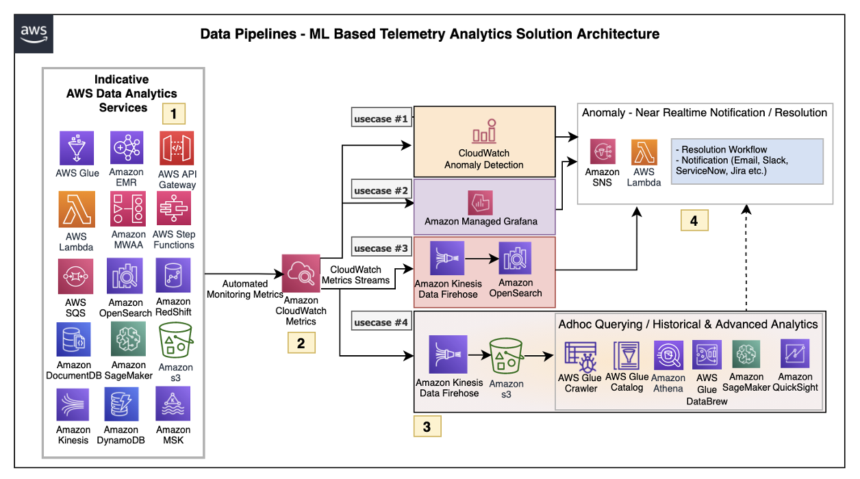
Figure 2. ML-based telemetry analytics solution architecture
Let’s explore each of the architecture steps in detail.
1. Indicative AWS data analytics services: Choose from a broad range of AWS analytics services, including data movement, data storage, data lakes, big data analytics, log analytics, and streaming analytics to business intelligence, ML, and beyond. This diagram shows a subset of these data analytics services. You may use one or a combination of many, depending on your use case.
2. Amazon CloudWatch metrics for telemetry analytics: Collecting and visualizing real-time logs, metrics, and event data is a key step in any process. CloudWatch helps you accomplish these tasks without any infrastructure provisioning. Almost every AWS data analytics service is integrated with CloudWatch to enable automatic capturing of the detailed metrics needed for telemetry analytics.
3. Near real-time use case examples: Step three presents practical, near real-time use cases that represent a range of real-world applications, one or more of which may apply to your own business needs.
Use case 1: Anomaly detection
CloudWatch provides the functionality to apply anomaly detection for a metric. The key business use case of this feature is to apply statistical and ML algorithms on a per-metrics basis of business critical applications to proactively identify issues and raise alarms.
The focus is on a single set of metrics that will be important for the application’s functioning—for example, AWS Lambda metrics of a 24/7 credit card company’s fraud monitoring application.
Use case 2: Unified metrics using Amazon Managed Grafana
For proper insights into telemetry data, it is important to unify metrics and collaboratively identify and troubleshoot issues in analytical systems. Amazon Managed Grafana helps to visualize, query, and corelate metrics from CloudWatch in near real-time.
For example, Amazon Managed Grafana can be used to monitor container metrics for Amazon EMR running on Amazon Elastic Kubernetes Service (Amazon EKS), which supports processing high-volume data from business critical Internet of Things (IoT) applications like connected factories, offsite refineries, wind farms, and more.
Use case 3: Combined business and metrics data using Amazon OpenSearch Service
Amazon OpenSearch Service provides the capability to perform near real-time, ML-based interactive log analytics, application monitoring, and search by combining business and telemetry data.
As an example, customers can combine AWS CloudTrail logs for AWS logins, Amazon Athena, and Amazon RedShift query access times with employee reference data to detect insider threats.
This log analytics use case architecture integrates into OpenSearch, as in Figure 3.

Figure 3. Log analytics use case architecture overview with OpenSearch
Use case 4: ML-based advanced analytics
Using Amazon Simple Storage Service (Amazon S3) as data storage, data lake customers can tap into AWS analytics services such as the AWS Glue Catalog, AWS Glue DataBrew, and Athena for preparing and transforming data, as well as build trend analysis using ML models in Amazon SageMaker. This mechanism helps with performing ML-based advanced analytics to identify and resolve recurring issues.
4. Anomaly resolution: When an alert is generated either by CloudWatch alarm, OpenSearch, or Amazon Managed Grafana, you have the option to act on the alert in near-real time. Amazon Simple Notification Service (Amazon SNS) and Lambda can help build workflows. Lambda also helps integrate with ServiceNow ticket creation, Slack channel notifications, or other ticketing systems.
Simple data pipeline example
Let’s explore another practical example using an architecture that demonstrates how AWS Step Functions orchestrates Lambda, AWS Glue jobs, and crawlers.
To report an anomaly on AWS Glue jobs based on total number of records processed, you can leverage the glue.driver.aggregate.recordsRead CloudWatch metric and set up a CloudWatch alarm based on anomaly detection, Amazon SNS topic for notifications, and Lambda for resolution, as in Figure 4.
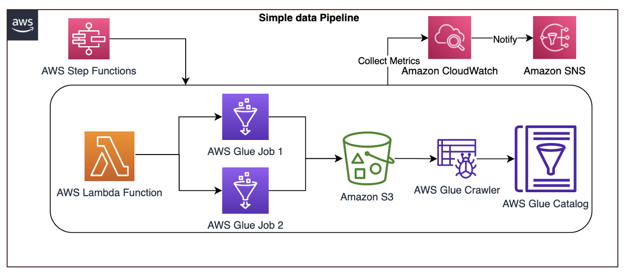
Figure 4. AWS Step Functions orchestrating Lamba, AWS Glue jobs, and crawlers
Here are the steps involved in the architecture proposed:
- CloudWatch automatically captures the metric
glue.driver.aggregate.recordsReadfrom AWS Glue jobs. - Customers set a CloudWatch alarm based on the anomaly detection of
glue.driver.aggregate.recordsReadmetric and set a notification to Amazon SNS topic. - CloudWatch applies a ML algorithm to the metric’s past data and creates a model of metric’s expected values.
- When the number of records increases significantly, the metric from the CloudWatch anomaly detection model notifies the Amazon SNS topic.
- Customers can notify an email group and trigger a Lambda function to resolve the issue, or create tickets in their operational monitoring system.
- Customers can also unify all the AWS Glue metrics using Amazon Managed Grafana. Using Amazon S3, data lake customers can crawl and catalog the data in the AWS Glue catalog and make it available for ad-hoc querying. Amazon SageMaker can be used for custom model training and inferencing.
Conclusion
In this blog post, we covered a recommended architecture to enable near-real time telemetry analytics for data pipelines, anomaly detection, notification, and resolution. This provides resiliency to the customer applications by proactively identifying and resolving issues.
Документален филм 151 г. от рождението на Гоце Делчев – огромен срам за България, от който имахме нужда
Post Syndicated from Милва Цветкова original https://bivol.bg/milva_tsvetkova_goce_delchev.html
петък 3 март 2023

Този документален материал беше създаден, за да запечата градацията на случилото се в Скопие по време на честването на рождението на Гоце Делчев през 2023 г. Фактите и обстоятелствата, документирани…
1945 Battle for Manila
Post Syndicated from The History Guy: History Deserves to Be Remembered original https://www.youtube.com/watch?v=U2eYrWwBN_0
What’s Up, Home? – Follow the news
Post Syndicated from Janne Pikkarainen original https://blog.zabbix.com/whats-up-home-follow-the-news/25497/
Can you follow the news with Zabbix? Of course, you can! By day, I am a lead site reliability engineer at a global cyber security company. By night, I monitor my home with Zabbix & Grafana and do some weird experiments with them. Welcome to my blog about the project.
A long time ago, before the dawn of social media, RSS (Really Simple Syndication) readers were all the rave. Instead of visiting each site you followed individually, you could add their RSS feeds to your RSS reader, which then would show you the latest news titles from as many sources as you wanted. Not only the titles, but depending on the news site you could also read a teaser or even the full news through your RSS reader without ever visiting the site itself.
Is RSS still a thing?
This was all good for the end-users, but the beancounters at the news companies got worried, as of course without visits to news sites, the advertisement income would come down, too. RSS readers can still be useful, but…. oh, I’ll need to stop, this is not the scope of this blog post.
Instead, the underlying technology of RSS is what makes it interesting. It’s just XML, so easy to consume by whatever software. Even though RSS is not a media darling anymore, it’s useful for gathering info from various sources to be then utilized somewhere else — like in Zabbix.
Let’s follow this site
So, how to follow the latest posts on this site through Zabbix? Easy, as this is just about parsing some XML.

Let’s begin with adding a new HTTP agent item.

With that in place, let’s add some dependent items, with the end result being this:

Each of those is just dependent items with some item pre-processing — the example below parses the first occurrence of title to the text.

How to use this?
In this case, I created a separate dashboard to show the latest blog post title, a link to it and the publication date. Wouldn’t be too hard to create a custom Zabbix module to make this fancier, but let’s leave it for another day. For now, by just using Item value widget types, we get this.

In the real world, there are plenty of actual use cases. Use it to alert you about the latest vulnerabilities, updates or other news about the stuff you have in your environment. Create a news dashboard for your security operations team or developers. If your own products do utilize RSS for something, this also can be very handy for end-to-end testing, as both Zabbix and your eyes can spot visually if something is not right. I’m sure you can come up with more and better ideas.
I have been working at Forcepoint since 2014 and never get tired of the news. — Janne Pikkarainen
This post was originally published on the author’s page.
Има ли кой? Има ли как? А могат ли?
Post Syndicated from Емилия Милчева original https://www.toest.bg/ima-li-koi-ima-li-kak-a-mogat-li/

Изборите така зачестиха, че партиите дори не си правят труда да предлагат нови послания и предизборни платформи. Че какво им е на старите – винаги и по всяко време се оферират справедлива държава, нов асфалт и европейски доходи.
В навечерието на поредните избори на 2 април няма лозунги за ред в хаоса, гонене на мутри и „всякая сволочь“, за пунически войни с корупцията и единство на нацията. След провалите в 48-мия парламент и предстоящия за две години пети вот политическата патетика би изглеждала по-скоро карнавална, отколкото нахъсваща и мобилизираща.
Проблемът с мигрантите заради охраната на българо-турската граница измести темата за Шенген. Провалът в подготовката за еврозоната отложи темата за еврото, но не и страховете, разпалвани от „Възраждане“, БСП и други проруски сили, за бум на цените и обедняване. Така две смислени и важни за българското бъдеще в ЕС цели изпаднаха от предизборната кампания.
Темата за корупцията започна да придобива по-ясни очертания с втория списък със санкции по Глобалния акт „Магнитски“, проверките на Европейската прокуратура на манипулациите с парникови емисии, свързани с империята на Христо Ковачки, и публично обявените разкрития на служебния кабинет, че асфалтът по Северната тангента е 14 см вместо 20. В строителството на 17-километровата магистрална отсечка за 220 млн. лв. са все предпочитани при управленията на ГЕРБ строители – консорциум ХПВС–ССТ, в който участват „Водстрой 98“, „Хидрострой“ АД, „Пътни строежи Велико Търново“ АД, „Пътинженерингстрой“ АД и „Пътстрой Бургас“. Прокурорите на Лаура Кьовеши проверяват още един спорен ремонт – този на „Графа“, и качеството на изпълнението му, предизвикало вълна от критики и сарказъм преди време. Изпълнител на ремонта на Зона 2 от центъра на София на стойност 20 113 417 лв. без ДДС е друг фаворит на ГЕРБ – „Джи Пи Груп“.
(Ако правителството на президента продължи да вади нови факти за най-свидното на Борисов – пътищата, значи ли, че краткият флирт между него и Радев е приключил?)
Няма обаче предложения за решения на най-тежкия за мнозина българи проблем – поскъпването на храните. За българските пенсионери, работещите бедни, уязвимите малцинствени групи това е жизненоважно.
Главен прокурор vs. високи цени на храните
Годишната инфлация на хранителните стоки е 24,5 % през януари, обяви на 2 март служебният земеделски министър Явор Гечев, като съобщи за „нелоялни търговски практики“, в т.ч. много големи маржове между цените на едро и дребно, достигащи до 90%. „Очеизвадно високи цени, които не са оправдани и водят до необосновано високи печалби“, както обясни Гечев по Нова телевизия. Как ще се справят политическите сили с овладяването на твърде скъпите храни в търговските вериги – служебният кабинет наблюдава и съобщава, ами редовният?
Остарелият Закон за защита на потребителите се нуждае от сериозни промени, както и този за защита на конкуренцията, а самата Комисия за защита на конкуренцията (КЗК) – от нов състав, който коалиционното правителство на „Промяната“ не свари да избере. Картелите са отдавнашен проблем на малкия български пазар, но доказването им е трудно и изисква, освен политическа воля, и по-прецизни нормативни разпоредби. Например да се даде възможност за внезапни проверки, тъй като сегашният закон изисква съдебно разрешение за инспекции на КЗК, а това означава и уведомяване на съответната компания от страна на съда. Тази законова разпоредба силно намалява вероятността да се намерят съответните доказателства.
Никоя от партиите с шанс за мандат за правителство в 49-тия парламент обаче не дава сигнали, че обмисля комплексни мерки за овладяване на високите цени на храните. Единствено БСП, която твърди, че е социална, обяви, че ще внесе незабавно в бъдещото Народно събрание законопроект за таван на цените на основните хранителни стоки. От новосформираната коалиция „Левицата“ веднага конкурираха с предложение за таван на надценките на 10 основни храни. ДПС, чиито избиратели са сред най-засегнатите от поскъпването, поставя инфлацията като основна тема в предизборната си кампания, без да назовава мерки за справяне, но слага на масата също и „дълбока конституционна реформа на съдебната система“, както каза Йордан Цонев.
Курс за такава реформа са обявили и ГЕРБ, и ПП, и ДБ. Известно е, че възгледите им се различават, независимо от заявката на Бойко Борисов в „Лице в лице“ по bTV, че този път ГЕРБ ще подкрепи законопроекта на служебния правосъден министър Крум Зарков за промени в Закона за съдебната власт, за да се въведе механизъм за разследване на главния прокурор. Но пък побърза да каже, че после трябва да се произнесе Конституционният съд.
На политическия фронт
ГЕРБ–СДС и „Продължаваме промяната – Демократична България“ са в схватка за първото място, ДПС и „Възраждане“ си оспорват третото, за БСП – каквото остане. „Български възход“, тази невзрачна политическа сила, която се запомни с поддакването си в 48-мия парламент, този път може и да не получи ударна инжекция гласове в последните часове на изборния ден, след като доскорошните ѝ партньори – Партията на зелените и Съюзът на свободните демократи – се оттеглиха от съвместно участие за 2 април.
Провалиха се и преговорите с ВМРО, а АБВ на Румен Петков, декларирала подкрепа за БВ на миналия вот, се вля в коалиция „Левицата“ заедно с други отломки от БСП. Но същинският удар дойде от проверката на Европейската прокуратура по енергийни предприятия, свързвани с Христо Ковачки, сочен и като спонсора за(д) „Български възход“.
„Има такъв народ“, която изпадна от 48-мия парламент, НДСВ, „Левицата“, новата коалиция „Заедно“ на бившите славитрифоновци Ива Митева и Любомир Каримански ще се борят ако не за парламент, за партийна субсидия.
Засега изглежда, че въпреки раздорите при сглобяването на листите, коалицията ПП–ДБ привлича разнородна подкрепа – от „Републиканци за България“, партията на някогашния Втори в ГЕРБ Цветан Цветанов, от БЗНС и „Обединени земеделци“.
Въпросът на въпросите
Големият въпрос за 2 април и всички избори след войната в Украйна, която промени света, не е кой ще е първи и ще успее ли да състави редовно правителство. Въпросът на въпросите е какво бъдеще за държавата България и нейните граждани предлагат политическите сили.
На този въпрос не могат да отговорят. Разбира се, могат да измрънкат извинения като „нека видим резултатите“ или „зависи от…“. Същинската беда е, че нямат отговор, защото липсват визия и визионери, защото мислят в плиткия обхват на тяснопартийни цели, защото ги спъват лобистки интереси, защото не знаят как да се справят с големите и трайно нерешени проблеми в демографията, здравеопазването и образованието. Затова и ги избягват по време на управлението си – в замяна добавят по някоя и друга стратегия в килограмите празнословие и им наливат още милиони.
Ако партиите са неспособни да разкажат бъдещето, избирателите ще им разкажат играта.
На второ четене: „Един ден в музея“
Post Syndicated from Севда Семер original https://www.toest.bg/na-vtoro-chetene-edin-den-v-muzeya/
„Един ден в музея“ от Тодор Петев и Зорница Христова, илюстрации Сияна Захариева
изд. „Точица“, 2021

Докато четях „Един ден в музея“ – гид за най-известните музеи в София под формата на комикс, – си спомних за първия път, когато от училище организираха посещение на Националния исторически музей.
Тъкмо бяха открили метрото в София и учителите ни бяха решили да се възползват, за да ни заведат. От нас само едно дете беше пътувало, така че, след като обявиха новината за музея, въпросният съученик се провикна – искаше да ни съобщи важна информация. Ако не си внимателен и не си пазиш добре краката, предупреди той, метрото ще ти ги пореже.
До днес не знам откъде се появи тази история, но тогава я приех сериозно – и въображението ми взе да работи. С онази запазена за детството смесица от неописуем ужас и любопитство зачаках деня на посещението. Опитвах се да си представя как точно става порязването, и още помня всички сценарии, за които исках да бъда подготвена. Най-вероятно ми се струваше метрото да няма под – тоест трябваше да си държиш краката изправени, щом седнеш. За всеки случай тренирах след училище.
Щом денят настъпи, бях заета през цялото време да си отварям очите на четири, за да не пропусна точно къде и как се случва порязването. Помня и разочарованието, че нищо такова не видях. А пък от самия музей нямам абсолютно никакъв спомен.
Докато четях книгата на Зорница Христова и Тодор Петев с илюстрации от Сияна Захариева, се замислих каква организация е била направена в онзи отдавнашен ден – учителите безопасно да заведат двайсетина малки деца до сградата на музея, да планират какво точно да им покажат вътре, какво да им разкажат, като се погрижат всяко дете да получи храна, вода и внимание. А пък аз съм си представяла и предвкусвала нещо страшно и интересно, което до такава степен е занимавало въображението ми, че самото посещение в музея, заради което изобщо сме били в метрото, е потънало някъде в паметта ми.
Именно напасването на реалността с въображението е идейният център на книжката. Още с предговора тя се обръща едновременно и към децата, и към родителите, но с пълното съзнание, че малките читатели не обичат тези въвеждащи страници. Така че основното обяснение за това каква е книгата, е към родителя; на детето му се предлага да разгледа картинките и да реши къде иска да отиде. Това ми се стори много хубаво – да позволиш на детето да следва собствените си интереси, което веднага представя
музея като терен за изследване, а не като още едно място, на което да слушаш урок.

„Един ден в музея“ е разделен на кратки глави, всяка от които – посветена на различен музей. Тук са „Квадрат 500“, Политехническият музей, дори Ботаническата градина – все интригуващи места. От всяко обаче са представени малък брой предмети, което може да изглежда странно – все пак нали това е хубавото на музея, разнообразието. Авторите обясняват, че
за децата нещата в един музей са твърде много, за да бъдат осмислени.
Затова тук основната нишка, скрепяваща всяка глава, са забавните и любопитни истории.
Водачи из различните музеи са необичайни герои – от учени до солници и други предмети и растения. Всяка глава приключва и с хубав списък от идеи как ученето да продължи. Всяко дете може да се почувства включено в разнообразни дейности: за някои би било интересно да направят експеримент, за други – да прочетат нещо допълнително, за трети – да идат в друг музей, където да открият свързани предмети. Авторите казват в предговора си, че са се опитали да активират всички сетива на децата, което много ми хареса – ученето все пак не е само интелектуална дейност, понякога трябва и да опиташ сам да си направиш сол.
Тази книга е една карта със съкровища, която може да отведе детето до всякакви дестинации. По този мил начин
музеят се превръща в пространство за игра.
Струва ми се, че немалко хора приемат музеите твърде сериозно – без да искам да звуча, сякаш обвинявам някого. Знам, че това идва от уважение, понякога към историята, друг път – към работата на онези, които са събрали експонатите.
Вярвам обаче, че най-хубавият начин да покажем уважение е да превърнем музея именно в площадка за игра. Важи и за възрастните. За мен беше страшно интересно да прочета напълно нови неща за любими музеи, в които съм била десетки пъти. Не използвам с лекота думата „вдъхновение“, но мисля, че в тази книга тя се изпълва със смисъл. Пътеводителят може да се използва дни наред, за да се посетят различни места. Полезно е, че се предлагат и по-общи инструменти за събуждане на любопитството – например описан е забавен начин да се четат картини, което е чудесно.
Може би най-важното от всичко е, че голяма част от въздействието на тази книга дава плодове във въображението на детето още преди то да стигне до музея. И малките посетители се превръщат в част от онова, което предстои да видят. Именно така се задейства магията на едно такова място: децата, застанали сред паметниците на културното наследство, създават лична връзка с тях. Връзка, която поражда спомени.


Красивите рисунки на Сияна Захариева също са превърнати в площадка за игра, например подканят детето да ги оцвети. Всичко в книгата е живо – от гаджета дървета до скелети, които се оплакват от домашното си. Хуморът е важна част, която също олекотява очакванията и изживяванията в музея. Съвсем позволено е, оказва се, да се смеем в тези сериозни и тихи зали.
Току-що излезе и втората част на този чудесен проект – казва се „Още един ден в музея“.
Първата част спечели „Златен лъв“ за издателски проект с най-голяма обществена значимост. Лично аз се надявам поредицата да продължи, да се развива, даже да заеме цяла лавица. Все пак музеите са пълни с истории, а децата – с любопитство. Затова можеш да посещаваш любимата си зала или любимата си картина в различни възрасти, сезони, настроения, да гледаш как собственият ти поглед променя това, което виждаш, а то на свой ред променя теб самия. Независимо дали си малък, или голям. Защото музеите принадлежат на всички – поне за мен това е най-важното съобщение в тази книга.
Активните дарители на „Тоест“ получават постоянна отстъпка в размер на 20% от коричната цена на всички заглавия от каталога на „Точица“, както и на няколко други български издателства в рамките на партньорската програма Читателски клуб „Тоест“. За повече информация прочетете на toest.bg/club.
Никой от нас не чете единствено най-новите книги. Тогава защо само за тях се пише? „На второ четене“ е рубрика, в която отваряме списъците с книги, публикувани преди поне година, четем ги и препоръчваме любимите си от тях. Рубриката е част от партньорската програма Читателски клуб „Тоест“. Изборът на заглавия обаче е единствено на авторите – Стефан Иванов и Севда Семер, които биха ви препоръчали тези книги и ако имаше как веднъж на две седмици да се разходите с тях в книжарницата.
You Need to Learn This! Cloudflare Tunnel Easy Tutorial
Post Syndicated from Crosstalk Solutions original https://www.youtube.com/watch?v=ZvIdFs3M5ic
Obituary Editor
Post Syndicated from original https://xkcd.com/2745/

Access Amazon Athena in your applications using the WebSocket API
Post Syndicated from Abhi Sodhani original https://aws.amazon.com/blogs/big-data/access-amazon-athena-in-your-applications-using-the-websocket-api/
Modern applications are built with modular independent components or microservices that rely on an API framework to communicate with services. Many organizations are building data lakes to store and analyze large volumes of structured, semi-structured, and unstructured data. In addition, many teams are moving towards a data mesh architecture, which requires them to expose their data sets as easily consumable data products. To accomplish this on AWS, organizations use Amazon Simple Storage Service (Amazon S3) to provide cheap and reliable object storage to house their datasets. To enable interactive querying and analyzing their data in place using familiar SQL syntax, many teams are turning to Amazon Athena. Athena is an interactive query service that is used by modern applications to query large volumes of data on an S3 data lake using standard SQL.
When working with SQL databases, application developers and business analysts are most familiar with simple permissions management and synchronous query-response protocols—if a user has permissions to submit a query, they do so and receive the results from the server when the query is complete. Directly accessing Athena APIs, for example when integrating with a custom web application, requires an AWS Identity and Access Management (IAM) role for the applications, and requires you to build a custom process to poll for query completion asynchronously. The IAM role needs access to run Athena API calls, as well as S3 permissions to retrieve the Athena output stored on Amazon S3. Polling for Athena query completion when performed at several intervals could result in increased latency from the client perspective.
In this post, we present a solution that can integrate with your front-end application to query data from Amazon S3 using an Athena synchronous API invocation. With this solution, you can add a layer of abstraction to your application on direct Athena API calls and promote the access using the WebSocket API developed with Amazon API Gateway. The query results are returned back to the application as Amazon S3 presigned URLs.
Overview of solution
For illustration purposes, this post builds a COVID-19 data lake with a WebSocket API to handle Athena queries. Your application can invoke the WebSocket API to pull the data from Amazon S3 using an Athena SQL query, and the WebSocket API returns the JSON response with the presigned Amazon S3 URL. The application needs to parse the JSON message to read the presigned URL, download the data to local, and report the data back to the front end.
We use AWS Step Functions to poll the Athena query run. When the query is complete, Step Functions invokes an AWS Lambda function to generate the presigned URL and send the request back to the application.
The application doesn’t require direct access to Athena, just access to invoke the API. When using this solution, you should secure the API following AWS guidelines. For more information, refer to Controlling and managing access to a WebSocket API in API Gateway.
The following diagram summarizes the architecture, key components, and interactions in the solution.

The application is composed of the WebSocket API in API Gateway, which handles the connectivity between the client and Athena. A client application using the framework can submit the Athena SQL query and get back the presigned URL containing the query results data. The workflow includes the following steps:
- The application invokes the WebSocket API connection.
- A Lambda function is invoked to initiate the connection. The connection ID is stored in an Amazon DynamoDB
- When the client application is connected, it can invoke the
runqueryaction, which invokes the RunQuery Lambda function. - The function first runs the Athena query.
- When the query is started, the function checks the status and uses Step Functions to track the query progress.
- Step Functions invokes the third Lambda function to read the processed Athena results and get the presigned S3 URL. Failed messages are routed to an Amazon Simple Notification Service (Amazon SNS) topic, which you can subscribe to.
- The presigned URL is returned to the client application.
- The connection is closed using the OnDisconnect function.
The RunQuery Lambda function runs the Athena query using the start_query_execution request:
The Amazon S3 presigned URL is generated by invoking the generate_presigned_url request with the bucket and key information that hosts the Athena results. The code hard codes the presigner expiration to 120 seconds, which is configurable in the function input parameter PreSignerExpireSeconds. See the following code:
Prerequisites
This post assumes you have the following:
- Access to an AWS account
- Permissions to create an AWS CloudFormation stack
- Permissions to create the following resources:
- AWS Glue catalog databases and tables
- API Gateway
- Lambda function
- IAM roles
- Step Functions state machine
- SNS topic
- DynamoDB table
Enable the WebSocket API
To enable the WebSocket API of API Gateway, complete the following steps:
- Configure the Athena dataset.
To make the data from the AWS COVID-19 data lake available in the Data Catalog in your AWS account, create a CloudFormation stack using the following template. If you’re signed in to your AWS account, the following page fills out most of the stack creation form for you. All you need to do is choose Create stack. For instructions on creating a CloudFormation stack, see Getting started with AWS CloudFormation.
You can also use an existing Athena database to query, in which case you need to update the stack parameters.
- Sign in to the Athena console.
If this is the first time you’re using Athena, you must specify a query result location on Amazon S3. For more information about querying and accessing the data from Athena, see A public data lake for analysis of COVID-19 data.
- Configure the WebSocket framework using the following page, which deploys the API infrastructure using AWS Serverless Application Model (AWS SAM).
- Update the parameters
pBucketNamewith the S3 bucket (in theus-east-2region) that stores the Athena results and also update the database if you want to query an existing database. - Select the check box to acknowledge creation of IAM roles and choose Deploy.
At a high level, these are the primary resources deployed by the application template:
- An API Gateway with routes to the connect, disconnect, and query Lambda functions. Note that the API Gateway deployed with this sample doesn’t implement authentication and authorization. We recommend that you implement authentication and authorization before deploying into a production environment. Refer to Controlling and managing access to a WebSocket API in API Gateway to understand how to implement these security controls.
- A DynamoDB table for tracking client connections.
- Lambda functions to manage connection states using DynamoDB.
- A Lambda function to run the query and start the step function. The function includes an associated IAM role and policies with permissions to Step Functions, the AWS Glue Data Catalog, Athena, AWS Key Management Service (AWS KMS), and Amazon S3. Note that the Lambda execution role gives read access to the Data Catalog and S3 bucket that you specify in the deployment parameters. We recommend that you don’t include a catalog that contains sensitive data without first understanding the impacts and implementing additional security controls.
- A Lambda function with associated permissions to poll for the query results and return the presigned URL to the client.
- A Step Functions state machine with associated permissions to run the polling Lambda function and send API notifications using Amazon SNS.
Test the setup
To test the WebSocket API, you can use wscat, an open-source command line tool.
- Install NPM.
- Install wscat:
- On the console, connect to your published API endpoint by running the following command. The full URI to use can be found on the AWS CloudFormation console by finding the
WebSocketURIoutput in theserverlessrepo-aws-app-athena-websocket-integrationstack that was deployed by the AWS SAM application you deployed previously.
- To test the
runqueryfunction, send a JSON message like the following example. This triggers the state machine to run your SQL query using Athena and, using Lambda, return an S3 presigned URL to your client, which you can access to download the query results. Note that the API accepts any valid Athena query. Additional query validation could be added to the internal Lambda function if desired.
- Copy the value for
pre-signed-urland enter it into your browser window to access the results.
The presigned URL provides you temporary credentials to download the query results. For more information, refer to Using presigned URLs. This process can be integrated into a front-end web application to automatically download and display the results of the query.
Clean up
To avoid incurring ongoing charges, delete the resources you provisioned by deleting the CloudFormation stacks CovidLakeStacks and serverlessrepo-AthenaWebSocketIntegration via the AWS CloudFormation console. For detailed instructions, refer to the cleanup sections in the starter kit README files in the GitHub repo.
Conclusion
In this post, we showed how to integrate your application with Athena using the WebSocket API. We have included a GitHub repo for you to understand the code and modify it per your application requirements, to get the full benefits of the solution. We encourage you to further explore the features of the API Gateway WebSocket API to add in security using authorizers, view live invocations using dashboards, and expand the framework for more routes on action request.
Let’s stay in touch via the GitHub repo.
About the Authors
 Abhi Sodhani is a Sr. AI/ML Solutions Architect at AWS. He helps customers with a wide range of solutions, including machine leaning, artificial intelligence, data lakes, data warehousing, and data visualization. Outside of work, he is passionate about books, yoga, and travel.
 Robin Zimmerman is a Data and ML Engineer with AWS Professional Services. He works with AWS enterprise customers to develop systems to extract value from large volumes of data using AWS data, analytics, and machine learning services. When he’s not working, you’ll probably find him in the mountains—rock climbing, skiing, mountain biking, or out on whatever other adventure he can dream up.
Use Apache Iceberg in a data lake to support incremental data processing
Post Syndicated from Flora Wu original https://aws.amazon.com/blogs/big-data/use-apache-iceberg-in-a-data-lake-to-support-incremental-data-processing/
Apache Iceberg is an open table format for very large analytic datasets, which captures metadata information on the state of datasets as they evolve and change over time. It adds tables to compute engines including Spark, Trino, PrestoDB, Flink, and Hive using a high-performance table format that works just like a SQL table. Iceberg has become very popular for its support for ACID transactions in data lakes and features like schema and partition evolution, time travel, and rollback.
Apache Iceberg integration is supported by AWS analytics services including Amazon EMR, Amazon Athena, and AWS Glue. Amazon EMR can provision clusters with Spark, Hive, Trino, and Flink that can run Iceberg. Starting with Amazon EMR version 6.5.0, you can use Iceberg with your EMR cluster without requiring a bootstrap action. In early 2022, AWS announced general availability of Athena ACID transactions, powered by Apache Iceberg. The recently released Athena query engine version 3 provides better integration with the Iceberg table format. AWS Glue 3.0 and later supports the Apache Iceberg framework for data lakes.
In this post, we discuss what customers want in modern data lakes and how Apache Iceberg helps address customer needs. Then we walk through a solution to build a high-performance and evolving Iceberg data lake on Amazon Simple Storage Service (Amazon S3) and process incremental data by running insert, update, and delete SQL statements. Finally, we show you how to performance tune the process to improve read and write performance.
How Apache Iceberg addresses what customers want in modern data lakes
More and more customers are building data lakes, with structured and unstructured data, to support many users, applications, and analytics tools. There is an increased need for data lakes to support database like features such as ACID transactions, record-level updates and deletes, time travel, and rollback. Apache Iceberg is designed to support these features on cost-effective petabyte-scale data lakes on Amazon S3.
Apache Iceberg addresses customer needs by capturing rich metadata information about the dataset at the time the individual data files are created. There are three layers in the architecture of an Iceberg table: the Iceberg catalog, the metadata layer, and the data layer, as depicted in the following figure (source).
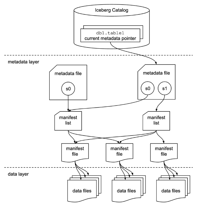
The Iceberg catalog stores the metadata pointer to the current table metadata file. When a select query is reading an Iceberg table, the query engine first goes to the Iceberg catalog, then retrieves the location of the current metadata file. Whenever there is an update to the Iceberg table, a new snapshot of the table is created, and the metadata pointer points to the current table metadata file.
The following is an example Iceberg catalog with AWS Glue implementation. You can see the database name, the location (S3 path) of the Iceberg table, and the metadata location.

The metadata layer has three types of files: the metadata file, manifest list, and manifest file in a hierarchy. At the top of the hierarchy is the metadata file, which stores information about the table’s schema, partition information, and snapshots. The snapshot points to the manifest list. The manifest list has the information about each manifest file that makes up the snapshot, such as location of the manifest file, the partitions it belongs to, and the lower and upper bounds for partition columns for the data files it tracks. The manifest file tracks data files as well as additional details about each file, such as the file format. All three files work in a hierarchy to track the snapshots, schema, partitioning, properties, and data files in an Iceberg table.
The data layer has the individual data files of the Iceberg table. Iceberg supports a wide range of file formats including Parquet, ORC, and Avro. Because the Iceberg table tracks the individual data files instead of only pointing to the partition location with data files, it isolates the writing operations from reading operations. You can write the data files at any time, but only commit the change explicitly, which creates a new version of the snapshot and metadata files.
Solution overview
In this post, we walk you through a solution to build a high-performing Apache Iceberg data lake on Amazon S3; process incremental data with insert, update, and delete SQL statements; and tune the Iceberg table to improve read and write performance. The following diagram illustrates the solution architecture.

To demonstrate this solution, we use the Amazon Customer Reviews dataset in an S3 bucket (s3://amazon-reviews-pds/parquet/). In real use case, it would be raw data stored in your S3 bucket. We can check the data size with the following code in the AWS Command Line Interface (AWS CLI):
The total object count is 430, and total size is 47.4 GiB.
To set up and test this solution, we complete the following high-level steps:
- Set up an S3 bucket in the curated zone to store converted data in Iceberg table format.
- Launch an EMR cluster with appropriate configurations for Apache Iceberg.
- Create a notebook in EMR Studio.
- Configure the Spark session for Apache Iceberg.
- Convert data to Iceberg table format and move data to the curated zone.
- Run insert, update, and delete queries in Athena to process incremental data.
- Carry out performance tuning.
Prerequisites
To follow along with this walkthrough, you must have an AWS account with an AWS Identity and Access Management (IAM) role that has sufficient access to provision the required resources.
Set up the S3 bucket for Iceberg data in the curated zone in your data lake
Choose the Region in which you want to create the S3 bucket and provide a unique name:
Launch an EMR cluster to run Iceberg jobs using Spark
You can create an EMR cluster from the AWS Management Console, Amazon EMR CLI, or AWS Cloud Development Kit (AWS CDK). For this post, we walk you through how to create an EMR cluster from the console.
- On the Amazon EMR console, choose Create cluster.
- Choose Advanced options.
- For Software Configuration, choose the latest Amazon EMR release. As of January 2023, the latest release is 6.9.0. Iceberg requires release 6.5.0 and above.
- Select JupyterEnterpriseGateway and Spark as the software to install.
- For Edit software settings, select Enter configuration and enter
[{"classification":"iceberg-defaults","properties":{"iceberg.enabled":true}}]. - Leave other settings at their default and choose Next.

- For Hardware, use the default setting.
- Choose Next.
- For Cluster name, enter a name. We use
iceberg-blog-cluster. - Leave the remaining settings unchanged and choose Next.
- Choose Create cluster.

Create a notebook in EMR Studio
We now walk you through how to create a notebook in EMR Studio from the console.
- On the IAM console, create an EMR Studio service role.
- On the Amazon EMR console, choose EMR Studio.
- Choose Get started.
The Get started page appears in a new tab.
- Choose Create Studio in the new tab.
- Enter a name. We use iceberg-studio.
- Choose the same VPC and subnet as those for the EMR cluster, and the default security group.
- Choose AWS Identity and Access Management (IAM) for authentication, and choose the EMR Studio service role you just created.
- Choose an S3 path for Workspaces backup.
- Choose Create Studio.
- After the Studio is created, choose the Studio access URL.
- On the EMR Studio dashboard, choose Create workspace.
- Enter a name for your Workspace. We use
iceberg-workspace. - Expand Advanced configuration and choose Attach Workspace to an EMR cluster.
- Choose the EMR cluster you created earlier.
- Choose Create Workspace.
- Choose the Workspace name to open a new tab.
In the navigation pane, there is a notebook that has the same name as the Workspace. In our case, it is iceberg-workspace.
- Open the notebook.
- When prompted to choose a kernel, choose Spark.
Configure a Spark session for Apache Iceberg
Use the following code, providing your own S3 bucket name:
This sets the following Spark session configurations:
- spark.sql.catalog.demo – Registers a Spark catalog named demo, which uses the Iceberg Spark catalog plugin.
- spark.sql.catalog.demo.catalog-impl – The demo Spark catalog uses AWS Glue as the physical catalog to store Iceberg database and table information.
- spark.sql.catalog.demo.warehouse – The demo Spark catalog stores all Iceberg metadata and data files under the root path defined by this property:
s3://iceberg-curated-blog-data. - spark.sql.extensions – Adds support to Iceberg Spark SQL extensions, which allows you to run Iceberg Spark procedures and some Iceberg-only SQL commands (you use this in a later step).
- spark.sql.catalog.demo.io-impl – Iceberg allows users to write data to Amazon S3 through S3FileIO. The AWS Glue Data Catalog by default uses this FileIO, and other catalogs can load this FileIO using the io-impl catalog property.
Convert data to Iceberg table format
You can use either Spark on Amazon EMR or Athena to load the Iceberg table. In the EMR Studio Workspace notebook Spark session, run the following commands to load the data:
After you run the code, you should find two prefixes created in your data warehouse S3 path (s3://iceberg-curated-blog-data/reviews.db/all_reviews): data and metadata.
Process incremental data using insert, update, and delete SQL statements in Athena
Athena is a serverless query engine that you can use to perform read, write, update, and optimization tasks against Iceberg tables. To demonstrate how the Apache Iceberg data lake format supports incremental data ingestion, we run insert, update, and delete SQL statements on the data lake.
Navigate to the Athena console and choose Query editor. If this is your first time using the Athena query editor, you need to configure the query result location to be the S3 bucket you created earlier. You should be able to see that the table reviews.all_reviews is available for querying. Run the following query to verify that you have loaded the Iceberg table successfully:
Process incremental data by running insert, update, and delete SQL statements:
Performance tuning
In this section, we walk through different ways to improve Apache Iceberg read and write performance.
Configure Apache Iceberg table properties
Apache Iceberg is a table format, and it supports table properties to configure table behavior such as read, write, and catalog. You can improve the read and write performance on Iceberg tables by adjusting the table properties.
For example, if you notice that you write too many small files for an Iceberg table, you can config the write file size to write fewer but bigger size files, to help improve query performance.
| Property | Default | Description |
| write.target-file-size-bytes | 536870912 (512 MB) | Controls the size of files generated to target about this many bytes |
Use the following code to alter the table format:
Partitioning and sorting
To make a query run fast, the less data read the better. Iceberg takes advantage of the rich metadata it captures at write time and facilitates techniques such as scan planning, partitioning, pruning, and column-level stats such as min/max values to skip data files that don’t have match records. We walk you through how query scan planning and partitioning work in Iceberg and how we use them to improve query performance.
Query scan planning
For a given query, the first step in a query engine is scan planning, which is the process to find the files in a table needed for a query. Planning in an Iceberg table is very efficient, because Iceberg’s rich metadata can be used to prune metadata files that aren’t needed, in addition to filtering data files that don’t contain matching data. In our tests, we observed Athena scanned 50% or less data for a given query on an Iceberg table compared to original data before conversion to Iceberg format.
There are two types of filtering:
- Metadata filtering – Iceberg uses two levels of metadata to track the files in a snapshot: the manifest list and manifest files. It first uses the manifest list, which acts as an index of the manifest files. During planning, Iceberg filters manifests using the partition value range in the manifest list without reading all the manifest files. Then it uses selected manifest files to get data files.
- Data filtering – After selecting the list of manifest files, Iceberg uses the partition data and column-level stats for each data file stored in manifest files to filter data files. During planning, query predicates are converted to predicates on the partition data and applied first to filter data files. Then, the column stats like column-level value counts, null counts, lower bounds, and upper bounds are used to filter out data files that can’t match the query predicate. By using upper and lower bounds to filter data files at planning time, Iceberg greatly improves query performance.
Partitioning and sorting
Partitioning is a way to group records with the same key column values together in writing. The benefit of partitioning is faster queries that access only part of the data, as explained earlier in query scan planning: data filtering. Iceberg makes partitioning simple by supporting hidden partitioning, in the way that Iceberg produces partition values by taking a column value and optionally transforming it.
In our use case, we first run the following query on the Iceberg table not partitioned. Then we partition the Iceberg table by the category of the reviews, which will be used in the query WHERE condition to filter out records. With partitioning, the query could scan much less data. See the following code:
Run the following select statement on the non-partitioned all_reviews table vs. the partitioned table to see the performance difference:
The following table shows the performance improvement of data partitioning, with about 50% performance improvement and 70% less data scanned.
| Dataset Name | Non-Partitioned Dataset | Partitioned Dataset |
| Runtime (seconds) | 8.20 | 4.25 |
| Data Scanned (MB) | 131.55 | 33.79 |
Note that the runtime is the average runtime with multiple runs in our test.
We saw good performance improvement after partitioning. However, this can be further improved by using column-level stats from Iceberg manifest files. In order to use the column-level stats effectively, you want to further sort your records based on the query patterns. Sorting the whole dataset using the columns that are often used in queries will reorder the data in such a way that each data file ends up with a unique range of values for the specific columns. If these columns are used in the query condition, it allows query engines to further skip data files, thereby enabling even faster queries.
Copy-on-write vs. read-on-merge
When implementing update and delete on Iceberg tables in the data lake, there are two approaches defined by the Iceberg table properties:
- Copy-on-write – With this approach, when there are changes to the Iceberg table, either updates or deletes, the data files associated with the impacted records will be duplicated and updated. The records will be either updated or deleted from the duplicated data files. A new snapshot of the Iceberg table will be created and pointing to the newer version of data files. This makes the overall writes slower. There might be situations that concurrent writes are needed with conflicts so retry has to happen, which increases the write time even more. On the other hand, when reading the data, there is no extra process needed. The query will retrieve data from the latest version of data files.
- Merge-on-read – With this approach, when there are updates or deletes on the Iceberg table, the existing data files will not be rewritten; instead new delete files will be created to track the changes. For deletes, a new delete file will be created with the deleted records. When reading the Iceberg table, the delete file will be applied to the retrieved data to filter out the delete records. For updates, a new delete file will be created to mark the updated records as deleted. Then a new file will be created for those records but with updated values. When reading the Iceberg table, both the delete and new files will be applied to the retrieved data to reflect the latest changes and produce the correct results. So, for any subsequent queries, an extra step to merge the data files with the delete and new files will happen, which will usually increase the query time. On the other hand, the writes might be faster because there is no need to rewrite the existing data files.
To test the impact of the two approaches, you can run the following code to set the Iceberg table properties:
Run the update, delete, and select SQL statements in Athena to show the runtime difference for copy-on-write vs. merge-on-read:
The following table summarizes the query runtimes.
| Query | Copy-on-Write | Merge-on-Read | ||||
| UPDATE | DELETE | SELECT | UPDATE | DELETE | SELECT | |
| Runtime (seconds) | 66.251 | 116.174 | 97.75 | 10.788 | 54.941 | 113.44 |
| Data scanned (MB) | 494.06 | 3.07 | 137.16 | 494.06 | 3.07 | 137.16 |
Note that the runtime is the average runtime with multiple runs in our test.
As our test results show, there are always trade-offs in the two approaches. Which approach to use depends on your use cases. In summary, the considerations come down to latency on the read vs. write. You can reference the following table and make the right choice.
| . | Copy-on-Write | Merge-on-Read |
| Pros | Faster reads | Faster writes |
| Cons | Expensive writes | Higher latency on reads |
| When to use | Good for frequent reads, infrequent updates and deletes or large batch updates | Good for tables with frequent updates and deletes |
Data compaction
If your data file size is small, you might end up with thousands or millions of files in an Iceberg table. This dramatically increases the I/O operation and slows down the queries. Furthermore, Iceberg tracks each data file in a dataset. More data files lead to more metadata. This in turn increases the overhead and I/O operation on reading metadata files. In order to improve the query performance, it’s recommended to compact small data files to larger data files.
When updating and deleting records in Iceberg table, if the read-on-merge approach is used, you might end up with many small deletes or new data files. Running compaction will combine all these files and create a newer version of the data file. This eliminates the need to reconcile them during reads. It’s recommended to have regular compaction jobs to impact reads as little as possible while still maintaining faster write speed.
Run the following data compaction command, then run the select query from Athena:
The following table compares the runtime before vs. after data compaction. You can see about 40% performance improvement.
| Query | Before Data Compaction | After Data Compaction |
| Runtime (seconds) | 97.75 | 32.676 seconds |
| Data scanned (MB) | 137.16 M | 189.19 M |
Note that the select queries ran on the all_reviews table after update and delete operations, before and after data compaction. The runtime is the average runtime with multiple runs in our test.
Clean up
After you follow the solution walkthrough to perform the use cases, complete the following steps to clean up your resources and avoid further costs:
- Drop the AWS Glue tables and database from Athena or run the following code in your notebook:
- On the EMR Studio console, choose Workspaces in the navigation pane.
- Select the Workspace you created and choose Delete.
- On the EMR console, navigate to the Studios page.
- Select the Studio you created and choose Delete.
- On the EMR console, choose Clusters in the navigation pane.
- Select the cluster and choose Terminate.
- Delete the S3 bucket and any other resources that you created as part of the prerequisites for this post.
Conclusion
In this post, we introduced the Apache Iceberg framework and how it helps resolve some of the challenges we have in a modern data lake. Then we walked you though a solution to process incremental data in a data lake using Apache Iceberg. Finally, we had a deep dive into performance tuning to improve read and write performance for our use cases.
We hope this post provides some useful information for you to decide whether you want to adopt Apache Iceberg in your data lake solution.
About the Authors
 Flora Wu is a Sr. Resident Architect at AWS Data Lab. She helps enterprise customers create data analytics strategies and build solutions to accelerate their businesses outcomes. In her spare time, she enjoys playing tennis, dancing salsa, and traveling.
 Daniel Li is a Sr. Solutions Architect at Amazon Web Services. He focuses on helping customers develop, adopt, and implement cloud services and strategy. When not working, he likes spending time outdoors with his family.
Visualize database privileges on Amazon Redshift using Grafana
Post Syndicated from Yota Hamaoka original https://aws.amazon.com/blogs/big-data/visualize-database-privileges-on-amazon-redshift-using-grafana/
Amazon Redshift is a fully managed, petabyte-scale data warehouse service in the cloud. Amazon Redshift enables you to use SQL for analyzing structured and semi-structured data with best price performance along with secure access to the data.
As more users start querying data in a data warehouse, access control is paramount to protect valuable organizational data. Database administrators want to continuously monitor and manage user privileges to maintain proper data access in the data warehouse. Amazon Redshift provides granular access control on the database, schema, table, column, row, and other database objects by granting privileges to roles, groups, and users from a SQL interface. To monitor privileges configured in Amazon Redshift, you can retrieve them by querying system tables.
Although Amazon Redshift provides a broad capability of managing access to database objects, we have heard from customers that they want to visualize and monitor privileges without using a SQL interface. In this post, we introduce predefined dashboards using Grafana which visualizes database privileges without writing SQL. This dashboard will help database administrators to reduce the time spent on database administration and increase the frequency of monitoring cycles.
Database security in Amazon Redshift
Security is the top priority at AWS. Amazon Redshift provides four levels of control:
- Cluster management
- Cluster connectivity
- Database access
- Temporary database credentials and single sign-on
This post focuses on database access, which relates to user access control against database objects. For more information, see Managing database security.
Amazon Redshift uses the GRANT command to define permissions in the database. For most database objects, GRANT takes three parameters:
- Identity – The entity you grant access to. This could be a user, role, or group.
- Object – The type of database object. This could be a database, schema, table or view, column, row, function, procedure, language, datashare, machine leaning (ML) model, and more.
- Privilege – The type of operation. Examples include CREATE, SELECT, ALTER, DROP, DELETE, and INSERT. The level of privilege depends on the object.
To remove access, use the REVOKE command.
Additionally, Amazon Redshift offers granular access control with the Row-level security (RLS) feature. You can attach or detach RLS policies to identities with the ATTACH RLS POLICY and DETACH RLS POLICY commands, respectively. See RLS policy ownership and management for more details.
Generally, database administrator monitors and reviews the identities, objects, and privileges periodically to ensure proper access is configured. They also need to investigate access configurations if database users face permission errors. These tasks require a SQL interface to query multiple system tables, which can be a repetitive and undifferentiated operation. Therefore, database administrators need a single pane of glass to quickly navigate through identities, objects, and privileges without writing SQL.
Solution overview
The following diagram illustrates the solution architecture and its key components:
- Amazon Redshift contains database privilege information in system tables.
- Grafana provides a predefined dashboard to visualize database privileges. The dashboard runs queries against the Amazon Redshift system table via the Amazon Redshift Data API.
Note that the dashboard focuses on visualization. SQL interface is required to configure privileges in Amazon Redshift. You can use query editor v2, a web-based SQL interface which enables users to run SQL commands from a browser.
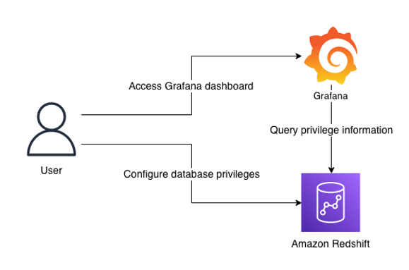
Prerequisites
Before moving to the next section, you should have the following prerequisites:
- An AWS account
- Create an Amazon Redshift cluster
- Setup Amazon Managed Grafana or local Grafana
- To setup with Amazon Managed Grafana, go through the following sections in Query and visualize Amazon Redshift operational metrics using the Amazon Redshift plugin for Grafana:
- Configure an Amazon Redshift cluster
- Configure an Amazon Managed Grafana workspace and sign in to Grafana
- Create a database user for Amazon Managed Grafana
- Configure a user in AWS SSO for Amazon Managed Grafana UI access
- Configure an Amazon Managed Grafana workspace and sign in to Grafana
- Set up an Amazon Redshift data source in Grafana
- To setup with local Grafana, first install Grafana following the official setup documentation. Next, go through the following sections in Query and visualize Amazon Redshift operational metrics using the Amazon Redshift plugin for Grafana:
- Create a database user for Amazon Managed Grafana
- Set up an Amazon Redshift data source in Grafana
- To setup with Amazon Managed Grafana, go through the following sections in Query and visualize Amazon Redshift operational metrics using the Amazon Redshift plugin for Grafana:
While Amazon Managed Grafana controls the plugin version and updates periodically, local Grafana allows user to control the version. Therefore, local Grafana could be an option if you need earlier access for the latest features. Refer to plugin changelog for released features and versions.
Import the dashboards
After you have finished the prerequisites, you should have access to Grafana configured with Amazon Redshift as a data source. Next, import two dashboards for visualization.
- In Grafana console, go to the created Redshift data source and click Dashboards
- Import the Amazon Redshift Identities and Objects
- Go to the data source again and import the Amazon Redshift Privileges
Each dashboard will appear once imported.
Amazon Redshift Identities and Objects dashboard
The Amazon Redshift Identities and Objects dashboard shows identites and database objects in Amazon Redshift, as shown in the following screenshot.
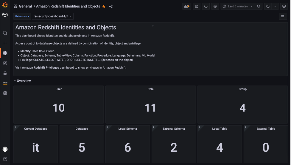
The Identities section shows the detail of each user, role, and group in the source database.
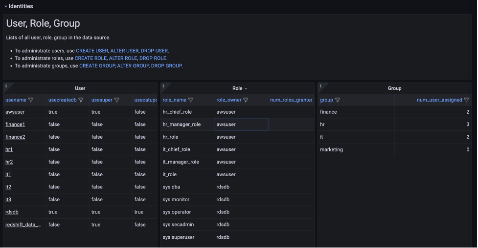
One of the key features in this dashboard is the Role assigned to Role, User section, which uses a node graph panel to visualize the hierarchical structure of roles and users from multiple system tables. This visualization can help administrators quickly examine which roles are inherited to users instead of querying multiple system tables. For more information about role-based access, refer to Role-based access control (RBAC).
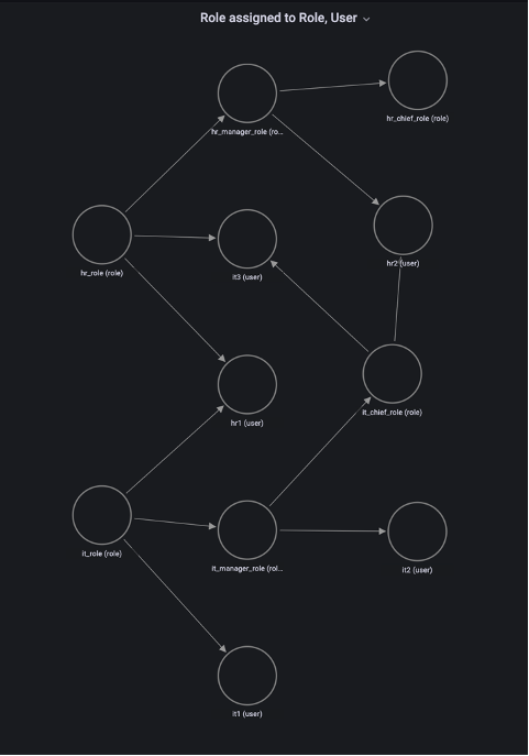
Amazon Redshift Privileges dashboard
The Amazon Redshift Privileges dashboard shows privileges defined in Amazon Redshift.
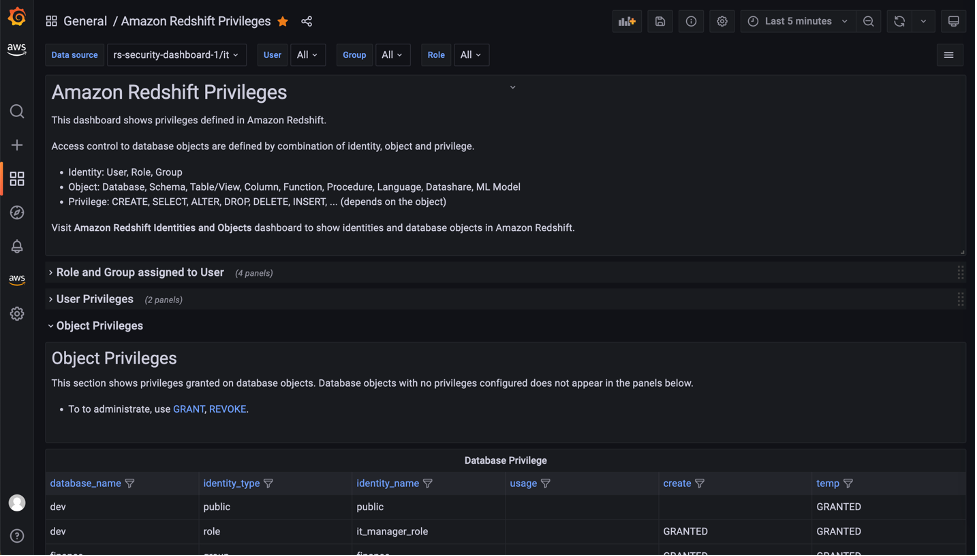
In the Role and Group assigned to User section, open the Role assigned to User panel to list the roles for a specific user. In this panel, you can list and compare roles assigned to multiple users. Use the User drop-down at the top of the dashboard to select users.
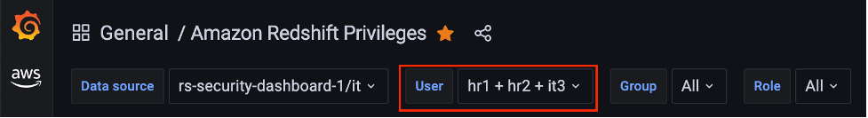
The dashboard will refresh immediately and show filtered result for selected users. Following screenshot is the filtered result for user hr1, hr2 and it3.
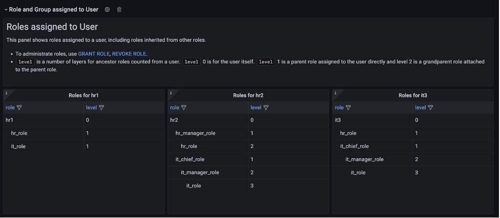
The Object Privileges section shows the privileges granted for each database object and identity. Note that objects with no privileges granted are not listed here. To show the full list of database objects, use the Amazon Redshift Identities and Objects dashboard.
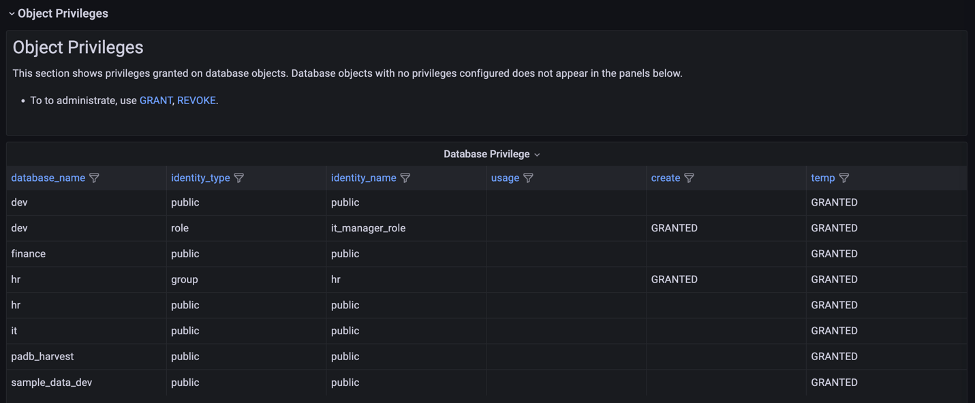
The Object Privileges (RLS) section contains visualizations for row-level security (RLS). The Policy attachments panel enables you to examine RLS configuration by visualizing relation between of tables, policies, roles and users.
Conclusion
In this post, we introduced a visualization for database privileges of Amazon Redshift using predefined Grafana dashboards. Database administrators can use these dashboards to quickly navigate through identities, objects, and privileges without writing SQL. You can also customize the dashboard to meet your business requirements. The JSON definition file of this dashboard is maintained as part of OSS in the Redshift data source for Grafana GitHub repository.
For more information about the topics described to in this post, refer to the following:
- Redshift data source for Grafana document
- Redshift data source for Grafana GitHub repository
- Monitor all your Redshift clusters in Grafana with the new Amazon Redshift data source plugin
- Query and visualize Amazon Redshift operational metrics using the Amazon Redshift plugin for Grafana
About the author

Yota Hamaoka is an Analytics Solution Architect at Amazon Web Services. He is focused on driving customers to accelerate their analytics journey with Amazon Redshift.