Post Syndicated from Amy Laresch original https://aws.amazon.com/blogs/big-data/aws-analytics-sales-team-uses-quicksight-q-to-save-hours-creating-monthly-business-reviews/
The AWS Analytics sales team is a group of subject-matter experts who work to enable customers to become more data driven through the use of our native analytics services like Amazon Athena, Amazon Redshift, and Amazon QuickSight. Every month, each sales leader is responsible for reporting on observations and trends in their business. To support their observations, the leaders track key metrics for their region as part of their monthly business review (MBR).
Today, sales leaders use a QuickSight dashboard to analyze these key metrics. Establishing a baseline is a time-intensive process that requires navigating various tabs and filters. To save time, analytics sales managers for the Americas regions have been eager to ask QuickSight Q, in their own business language, questions like “Who are my top customers by month-over-month revenue?” or “How much did Customer X spend on Amazon Redshift this month compared with last?”
Rather than manually filtering their views to understand the underlying signals, they now use the native capabilities of QuickSight Q, resulting in many hours saved per leader.
These sales leaders can instead focus on “why it happened” and “what’s coming next” (spoiler alert: Q supports “why?” and forecast questions).
Since each leader reports on the same metrics each month, they would like to save each QuickSight Q answer, curated for their region, so they can focus on growing their business. With QuickSight Q pinboards, they can do just that. They can pin visuals for one-click access to frequently asked questions. Every time the dataset updates, the visual will reflect the latest data, all of which gets rendered in seconds because of SPICE (Super-fast, Parallel, In-memory Calculation Engine).
The features explored in this post are part of Amazon QuickSight Q. Powered by machine learning (ML), Q uses natural language processing to answer your business questions quickly. If you’re an existing QuickSight user, be sure that the Q add-on is enabled. For steps on how to do this, see Getting started with Amazon QuickSight Q.
Personalized data for sales managers
Kellie Burton, Sr. QuickSight Solutions Architect, and Amy Laresch, a Product Manager for QuickSight Q, worked with sales leaders Patrick Callahan, US West, and Jeff Pratt, US Central, to build a QuickSight Q topic for Americas Analytics revenue. A topic is a collection of one or more datasets that represents a subject area that business users can ask questions about. The Americas Analytics topic is built on a revenue dataset that is protected with row-level security (RLS), so any question asked is restricted by the same rules.
To keep the topic focused and avoid potential language ambiguity, Kellie and Amy used copies of previous MBR deliverables to understand what measures, dimensions, and calculated fields were required in the topic. With QuickSight Q automated data prep, the calculated fields were automatically added to the topic, so the topic authors did not have to recreate them. With Q, readers could ask questions like “year-to-date (YTD) YoY % for us-west analytics by segment” to get the exact table view that Patrick includes in his MBR. During a usability session, the authors worked with Jeff and Patrick to ask Q each required question and save it to their pinboard.
After opening his completed pinboard, Jeff said, “Wow, that is really cool. It answers all the questions I write the MBR for in my own custom pinboard. A report that used to take me 2-3 hours to pull together will now only take me 5 minutes.” With the extra time, he’s energized to focus more on the story behind the data and planning for future.
Patrick shared Jeff’s sentiment saying, “This will be awesome for next month when I write my MBR. What previously took a couple of hours, I can now do in a few minutes. Now I can spend more time working to deliver my customer’s outcomes.”

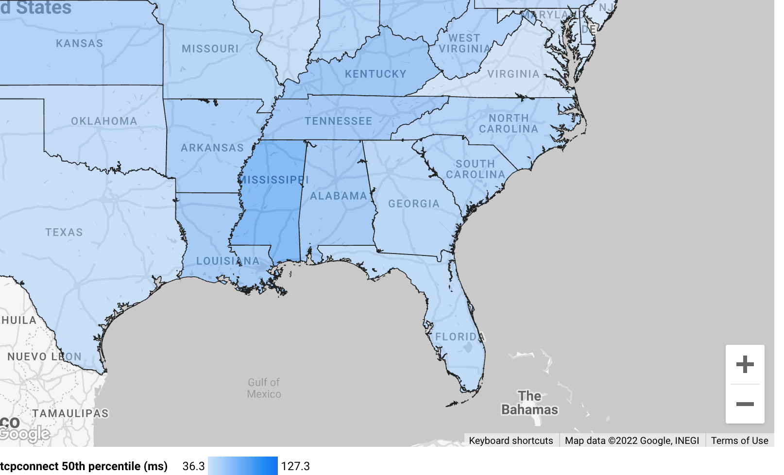
Sample pinboard for a sales leader for the Americas region with mock data (from the Software Sales sample topic)
Once you have an answer to a question, you might want to understand why that happened. This is where Q Why questions come into play.
Why questions
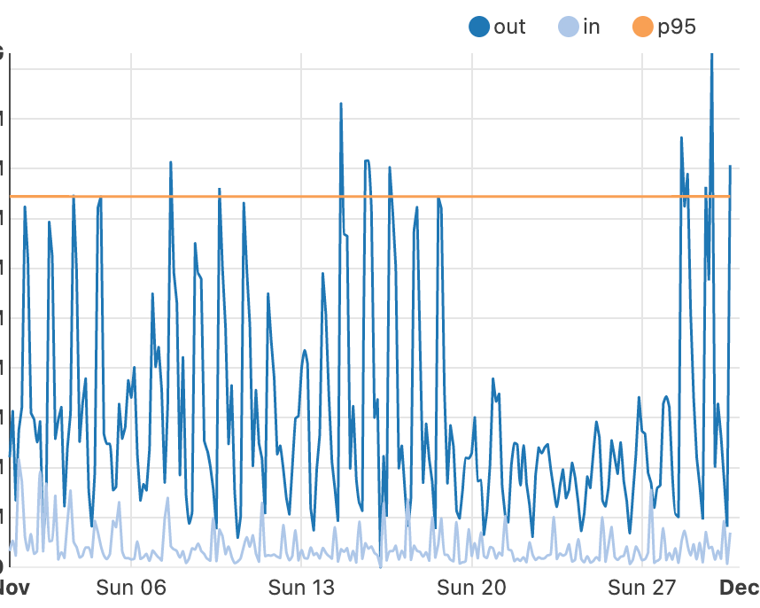
Understanding why is critical to making data-backed decisions to delight your customers and grow your business. For example, in this Software Sales sample topic, I asked Q for monthly revenue and noticed a drop in October 2022.

Mock data from the Software Sales sample topic
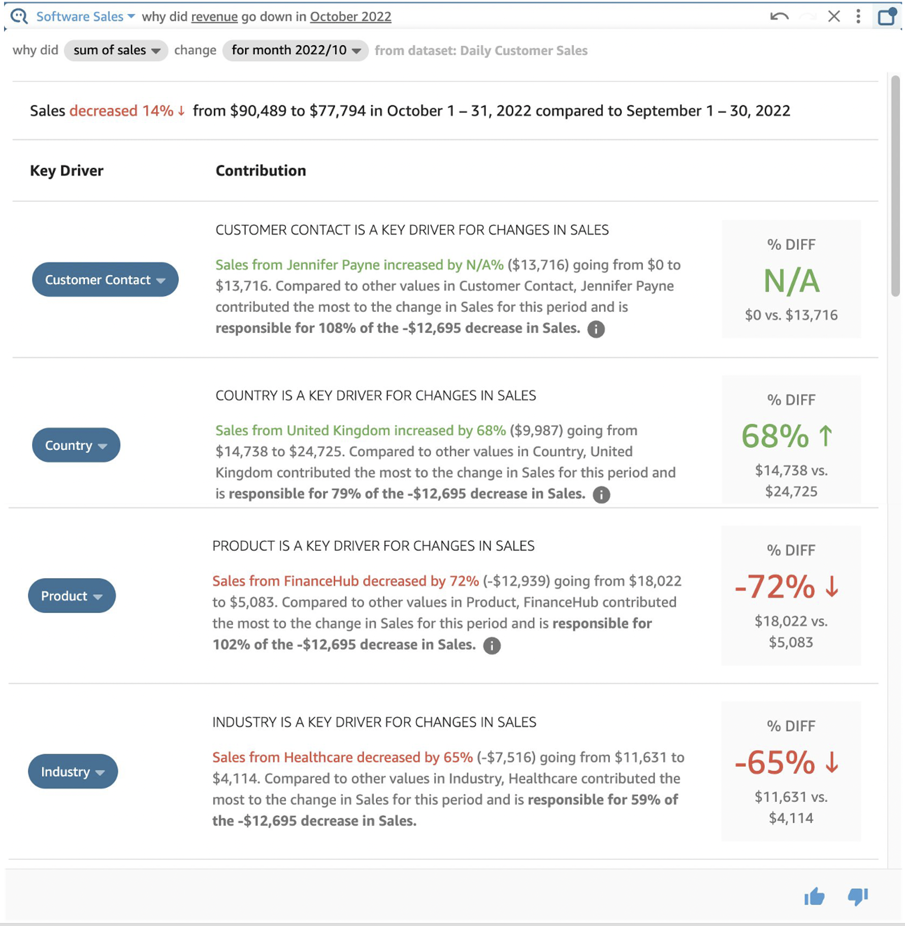
I ask Q, “Why?” and see four key drivers: Customer Contact, Country, Product, and Industry.
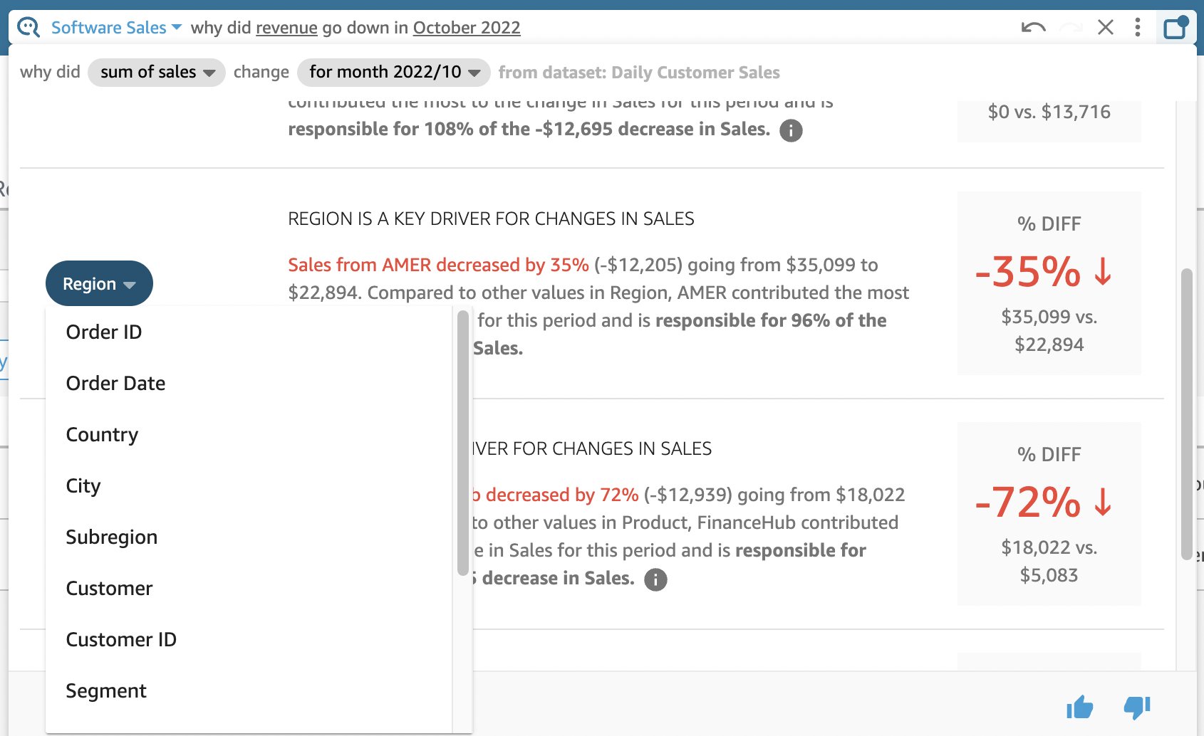
Next, I change Country to Region to see the impact at a higher level.
Forecast questions
Next, I can ask Q for a forecast that uses ML and factors, like seasonality, to predict the trend.

With pinboards, why questions, and forecast questions, QuickSight Q not only saves significant time and energy but delivers insights that previously required the help of an analyst or data scientist. Reflecting on the project, Kellie shared, “It’s been fun building on the bleeding edge of analytics. I’m so excited to see what Q will do in 2023!”
To learn more, watch What’s New for Readers with Amazon QuickSight Q and What’s New for Authors with Amazon QuickSight Q.
About the authors
 Amy Laresch is a product manager for Amazon QuickSight Q. She is passionate about analytics and is focused on delivering the best experience for every QuickSight Q reader. Check out her videos on the @AmazonQuickSight YouTube channel for best practices and to see what’s new for QuickSight Q.
 Kellie Burton is a Sr. Solutions Architect for Amazon QuickSight with over 25 years of experience in business analytics helping customers across a variety of industries. Kellie has a passion for helping customers harness the power of their data to uncover insights to make decisions.


 Al MS is a product manager for Amazon EMR at Amazon Web Services.