Tag Archives: Amazon OpenSearch Service

Building an event-driven solution for AvalonBay property leasing and search

Post Syndicated from Kausik Dey original https://aws.amazon.com/blogs/architecture/building-an-event-driven-solution-for-avalonbay-property-leasing-and-search/

In this blog post, we show you how to build an event-driven and serverless solution for property leasing and search that is scalable and resilient. This solution was created for AvalonBay Communities, Inc.—a leading residential Real Estate Investment Trusts (REITs). It enables:

  • More than 150,000 multi-parameter searches per day
  • The processing of more than 3,500 lease applications and 85,000 individual rent payments per month

Introduction

AvalonBay is an equity REIT. The company has a long track record of developing, redeveloping, acquiring, and managing apartment homes in top U.S. markets. AvalonBay builds long-term value for customers using innovative technology solutions.

The company understands that data-driven insights contribute to targeted business growth. But AvalonBay found that managing the complex interdependencies between multiple data sets—from real estate and property management systems to financial and payment systems—required a new solution.

The challenge

AvalonBay owned or held a direct or indirect ownership interest in 293 apartment communities containing 88,405 apartment homes in 12 states and Washington, D.C., as of September 30, 2022.

Of these, 18 communities were under development and one was under redevelopment. This presented a unique challenge to both internal and external users looking to search and lease apartment units based on multi-parameter selection criteria in geographically dispersed regions. For example, finding units in buildings with specific amenities, lease terms, furnishings and availability dates.

Overview of solution

AvalonBay’s fully managed leasing solution for applicants and residents is hosted by Amazon Web Services (AWS). The solution is secure, autoscaling, and multi-region, ensuring resiliency and performance with efficient resource usage.

In this event-driven solution, AvalonBay’s leasing service is hosted in multiple AWS Regions to provide low latency response to users across various geolocations. This blog post focuses on showing use case implementation in only one region—Region East— as shown in Figure 1.

AvalonBay lease processing platform

Figure 1. AvalonBay lease processing platform

Several AWS services come together in this solution to meet key company objectives. Let’s explore each one and its purpose within the architecture.

    1. Amazon Route 53: For AvalonBay’s Lease Processing solution, any non-transient service failure is unacceptable. In addition to providing a high degree of resiliency through a Multi-AZ architecture, Lease Processing also provides regional-level high availability through its multi-Region active-active architecture. Route 53 with latency-based routing allows dynamic rerouting of requests within seconds to alternate Regions.
    2. Amazon API Gateway: Route 53 latency-based routing is configured across multiple AWS Regions as Route 53 to route traffic to an API Gateway endpoint. API Gateway authorizers were added to control access to APIs using an Amazon Cognito user pool.
    3. AWS Lambda with provisioned concurrency: The Lambda services are set up for automatic scaling, secured through a private subnet, and span across Availability Zones. This provides horizontal scaling capability, self-healing capacity, and resiliency across Availability Zones. Provisioned concurrency minimizes the estimate of cold starts by generating execution environments. It also greatly reduces time spent on APIs invocations.
    4. Amazon Aurora V2 for Amazon Relational Database Service (Amazon RDS) PostgreSQL-Compatible Edition: Aurora Serverless V2 is an on-demand, autoscaling configuration for Aurora. Serverless Aurora V2 PostgreSQL-Compatible is used for the Lease Processing solution. The global database was configured with two Regions; us-east-1 as the primary cluster and us-west-2 as the secondary cluster. Automated Aurora global database endpoint management for planned and unplanned failover is configured through a Route 53 private hosted zone, Amazon EventBridge, and Lambda.
    5. Amazon RDS Proxy for Aurora: Amazon RDS Proxy allows the leasing application to pool and share database connections to improve its ability to scale. It also makes the leasing solution more resilient to database failures by automatically connecting to a standby database instance while preserving application connections.
    6. Amazon EventBridge: EventBridge supports the solution through two primary purposes:
      1. Oversees lease flow events – During the lease application process, the solution generates various events which are consumed by AvalonBay and external applications such as property management, finance portals, administration, and more. Leasing events are sent to EventBridge and various event rules are configured for multiple destinations including Lambda, Amazon Simple Notification Service (Amazon SNS), and external API endpoints.
      2. Handles global Aurora V2 failover – Aurora generates events when certain actions are taken or events occur, including any type of global database activity.
        • When a managed planned failover is initiated—either via the AWS Command Line Interface (AWS CLI), API, or console—the global database failover process starts and generates an event.
        • When an Aurora cluster is removed from a global cluster through the AWS CLI, API, or console, the Aurora cluster is promoted as a single primary cluster. Once this process is completed, it generates an event.

An EventBridge rule is created to match an event pattern any time a global database managed planned failover completes successfully in a Region. When a failover is completed, the completion event is detected, and this rule is triggered. The event rule is configured to invoke a Lambda function that is triggered on global database failover and updates the Amazon CloudFront CNAME record to the correct value.

Scalable search solution

Leasing professionals need to easily scan a huge amount of property information using AvalonBay’s Search Solution to obtain required information.

Using the Amazon OpenSearch Service, agents can generate property profiles and other asset data to identify matching units and quickly respond to end customers. OpenSearch is a fully open-source search and analytics engine that securely unlocks real-time search, monitoring, and analysis of business and operational data. It is employed for use cases such as application monitoring, log analytics, observability, and website search.

The AvalonBay Search Service solution architecture featuring OpenSearch is shown in Figure 2.

AvalonBay Search Service solution architecture

Figure 2: AvalonBay Search Service solution architecture

AvalonBay search requires search criteria including keyword and Universal Resource Identifier (URI) search, SQL-based search, and custom package search, all of which are detailed in the Amazon OpenSearch Service Developer Guide.

OpenSearch automatically detects and replaces failed OpenSearch Service nodes, reducing the overhead associated with self-managed infrastructures.

Let’s explore this architecture further by step.

  1. Amazon Kinesis event stream – The AvalonBay community requires near real-time updates to search attributes such as amenities, features, promotion, and pricing. Events created through various producers are streamed through Kinesis and inserted or updated through OpenSearch.
  2. Amazon OpenSearch – OpenSearch is used for end-to-end community search—a managed service making it easy to deploy, operate, and scale OpenSearch clusters in the AWS Cloud. As community search data is read-only, UltraWarm and cold storage are also used based on usage frequency.
  3. Amazon Simple Storage Service (S3): Various community documents, policies, and image or video files are key search elements. They must be maintained securely and reliably for years due to contractual obligations. Amazon S3 simplifies this task with high durabilitylifecycle rules, and varied controls for retention.

Conclusion

This post showed how AvalonBay has built and deployed custom leasing and search solutions on AWS serverless platforms without compromising resiliency, performance, and capacity requirements. This is a 24/7, fully managed solution with no additional equipment on-premises.

Choosing AWS for leasing and search solutions gives AvalonBay the ability to dynamically scale and meet future growth demands while introducing cost advantages. In addition, the global availability of AWS services makes it possible to deploy services across geographic locations to meet performance requirements.

Migrate your indexes to Amazon OpenSearch Serverless with Logstash

Post Syndicated from Prashant Agrawal original https://aws.amazon.com/blogs/big-data/migrate-your-indexes-to-amazon-opensearch-serverless-with-logstash/

We recently announced the general availability of Amazon OpenSearch Serverless , a new option for Amazon OpenSearch Service that makes it easy run large-scale search and analytics workloads without having to configure, manage, or scale OpenSearch clusters. With OpenSearch Serverless, you get the same interactive millisecond response times as OpenSearch Service with the simplicity of a serverless environment.

In this post, you’ll learn how to migrate your existing indices from an OpenSearch Service managed cluster domain to a serverless collection using Logstash.

With OpenSearch domains, you get dedicated, secure clusters configured and optimized for your workloads in minutes. You have full control over the configuration of compute, memory, and storage resources in clusters to optimize cost and performance for your applications. OpenSearch Serverless provides an even simpler way to run search and analytics workloads—without ever having to think about clusters. You simply create a collection and a group of indexes, and can start ingesting and querying the data.

Solution overview

Logstash is open-source software that provides ETL (extract, transform, and load) for your data. You can configure Logstash to connect to a source and a destination via input and output plugins. In between, you configure filters that can transform your data. This post walks you through the steps you need to set up Logstash to connect an OpenSearch Service domain (input) to an OpenSearch Serverless collection (output).

You set the source and destination plugins in Logstash’s config file. The config file has sections for Input, Filter, and Output. Once configured, Logstash will send a request to the OpenSearch Service domain and read the data according to the query you put in the input section. After data is read from OpenSearch Service, you can optionally send it to the next stage Filter for transformations such as adding or removing a field from the input data or updating a field with different values. In this example, you won’t use the Filter plugin. Next is the Output plugin. The open-source version of Logstash (Logstash OSS) provides a convenient way to use the bulk API to upload data to your collections. OpenSearch Serverless supports the logstash-output-opensearch output plugin, which supports AWS Identity and Access Management (IAM) credentials for data access control.

The following diagram illustrates our solution workflow.

Prerequisites

Before getting started, make sure you have completed the following prerequisites:

  1. Note down your OpenSearch Service domain’s ARN, user name, and password.
  2. Create an OpenSearch Serverless collection. If you’re new to OpenSearch Serverless, refer to Log analytics the easy way with Amazon OpenSearch Serverless for details on how to set up your collection.

Set up Logstash and the input and output plugins for OpenSearch

Complete the following steps to set up Logstash and your plugins:

  1. Download logstash-oss-with-opensearch-output-plugin. (This example uses the distro for macos-x64. For other distros, refer to the artifacts.)
    wget https://artifacts.opensearch.org/logstash/logstash-oss-with-opensearch-output-plugin-8.4.0-macos-x64.tar.gz

  2. Extract the downloaded tarball:
    tar -zxvf logstash-oss-with-opensearch-output-plugin-8.4.0-macos-x64.tar.gz
    cd logstash-8.4.0/

  3. Update the logstash-output-opensearch plugin to the latest version:
    <path/to/your/logstash/root/directory>/bin/logstash-plugin update logstash-output-opensearch

  4. Install the logstash-input-opensearch plugin:
    <path/to/your/logstash/root/directory>/bin/logstash-plugin install logstash-input-opensearch

Test the plugin

Let’s get into action and see how the plugin works. The following config file retrieves data from the movies index in your OpenSearch Service domain and indexes that data in your OpenSearch Serverless collection with same index name, movies.

Create a new file and add the following content, then save the file as opensearch-serverless-migration.conf. Provide the values for the OpenSearch Service domain endpoint under HOST, USERNAME, and PASSWORD in the input section, and the OpenSearch Serverless collection endpoint details under HOST along with REGION, AWS_ACCESS_KEY_ID, and AWS_SECRET_ACCESS_KEY in the output section.

input {
    opensearch {
        hosts =>  ["https://<HOST>:443"]
        user  =>  "<USERNAME>"
        password  =>  "<PASSWORD>"
        index =>  "movies"
        query =>  '{ "query": { "match_all": {}} }'
    }
}
output {
    opensearch {
        ecs_compatibility => disabled
        index => "movies"
        hosts => "<HOST>:443"
        auth_type => {
            type => 'aws_iam'
            aws_access_key_id => '<AWS_ACCESS_KEY_ID>'
            aws_secret_access_key => '<AWS_SECRET_ACCESS_KEY>'
            region => '<REGION>'
            service_name => 'aoss'
            }
        legacy_template => false
        default_server_major_version => 2
    }
}

You can specify a query in the input section of the preceding config. The match_all query matches all data in the movies index. You can change the query if you want to select a subset of the data. You can also use the query to parallelize the data transfer by running multiple Logstash processes with configs that specify different data slices. You can also parallelize by running Logstash processes against multiple indexes if you have them.

Start Logstash

Use the following command to start Logstash:

<path/to/your/logstash/root/directory>/bin/logstash -f <path/to/your/config/file>

After you run the command, Logstash will retrieve the data from the source index from your OpenSearch Service domain, and write to the destination index in your OpenSearch Serverless collection. When the data transfer is complete, Logstash shuts down. See the following code:

[2023-01-24T20:14:28,965][INFO][logstash.agent] Successfully
started Logstash API endpoint {:port=>9600, :ssl_enabled=>false}
…
…
[2023-01-24T20:14:38,852][INFO][logstash.javapipeline][main] Pipeline terminated {"pipeline.id"=>"main"}
[2023-01-24T20:14:39,374][INFO][logstash.pipelinesregistry] Removed pipeline from registry successfully {:pipeline_id=>:main}
[2023-01-24T20:14:39,399][INFO][logstash.runner] Logstash shut down.

Verify the data in OpenSearch Serverless

You can verify that Logstash copied all your data by comparing the document count in your domain and your collection. Run the following query either from the Dev tools tab, or with curl, postman, or a similar HTTP client. The following query helps you search all documents from the movies index and returns the top documents along with the count. By default, OpenSearch will return the document count up to a maximum of 10,000. Adding the track_total_hits flag helps you get the exact count of documents if the document count exceeds 10,000.

GET movies/_search
{
  "query": {
    "match_all": {}
  },
  "track_total_hits" : true
}

Conclusion

In this post, you migrated data from your OpenSearch Service domain to your OpenSearch Serverless collection using Logstash’s OpenSearch input and output plugins.

Stay tuned for a series of posts focusing on the various options available for you to build effective log analytics and search solutions using OpenSearch Serverless. You can also refer the Getting started with Amazon OpenSearch Serverless workshop to know more about OpenSearch Serverless.

If you have feedback about this post, submit it in the comments section. If you have questions about this post, start a new thread on the Amazon OpenSearch Service forum or contact AWS Support.


About the authors

Prashant Agrawal is a Sr. Search Specialist Solutions Architect with Amazon OpenSearch Service. He works closely with customers to help them migrate their workloads to the cloud and helps existing customers fine-tune their clusters to achieve better performance and save on cost. Before joining AWS, he helped various customers use OpenSearch and Elasticsearch for their search and log analytics use cases. When not working, you can find him traveling and exploring new places. In short, he likes doing Eat → Travel → Repeat.

Jon Handler (@_searchgeek) is a Sr. Principal Solutions Architect at Amazon Web Services based in Palo Alto, CA. Jon works closely with the CloudSearch and Elasticsearch teams, providing help and guidance to a broad range of customers who have search workloads that they want to move to the AWS Cloud. Prior to joining AWS, Jon’s career as a software developer included four years of coding a large-scale, eCommerce search engine.

Serverless logging with Amazon OpenSearch Service and Amazon Kinesis Data Firehose

Post Syndicated from Jon Handler original https://aws.amazon.com/blogs/big-data/serverless-logging-with-amazon-opensearch-service-and-amazon-kinesis-data-firehose/

In this post, you will learn how you can use Amazon Kinesis Data Firehose to build a log ingestion pipeline to send VPC flow logs to Amazon OpenSearch Serverless. First, you create the OpenSearch Serverless collection you use to store VPC flow logs, then you create a Kinesis Data Firehose delivery pipeline that forwards the flow logs to OpenSearch Serverless. Finally, you enable delivery of VPC flow logs to your Firehose delivery stream. The following diagram illustrates the solution workflow.

OpenSearch Serverless is a new serverless option offered by Amazon OpenSearch Service. OpenSearch Serverless makes it simple to run petabyte-scale search and analytics workloads without having to configure, manage, or scale OpenSearch clusters. OpenSearch Serverless automatically provisions and scales the underlying resources to deliver fast data ingestion and query responses for even the most demanding and unpredictable workloads.

Kinesis Data Firehose is a popular service that delivers streaming data from over 20 AWS services to over 15 analytical and observability tools such as OpenSearch Serverless. Kinesis Data Firehose is great for those looking for a fast and easy way to send your VPC flow logs data to your OpenSearch Serverless collection in minutes without a single line of code and without building or managing your own data ingestion and delivery infrastructure.

VPC flow logs capture the traffic information going to and from your network interfaces in your VPC. With the launch of Kinesis Data Firehose support to OpenSearch Serverless, it makes an easy solution to analyze your VPC flow logs with just a few clicks. Kinesis Data Firehose provides a true end-to-end serverless mechanism to deliver your flow logs to OpenSearch Serverless, where you can use OpenSearch Dashboards to search through those logs, create dashboards, detect anomalies, and send alerts. VPC flow logs helps you to answer questions like:

  • What percentage of your traffic is getting dropped?
  • How much traffic is getting generated for specific sources and destinations?

Create your OpenSearch Serverless collection

To get started, you first create a collection. An OpenSearch Serverless collection is a logical grouping of one or more indexes that represent an analytics workload. Complete the following steps:

  1. On the OpenSearch Service console, choose Collections under Serverless in the navigation pane.
  2. Choose Create a collection.
  3. For Collection name, enter a name (for example, vpc-flow-logs).
  4. For Collection type¸ choose Time series.
  5. For Encryption, choose your preferred encryption setting:
    1. Choose Use AWS owned key to use an AWS managed key.
    2. Choose a different AWS KMS key to use your own AWS Key Management Service (AWS KMS) key.
  6. For Network access settings, choose your preferred setting:
    1. Choose VPC to use a VPC endpoint.
    2. Choose Public to use a public endpoint.

AWS recommends that you use a VPC endpoint for all production workloads. For this walkthrough, select Public.

  1. Choose Create.

It should take couple of minutes to create the collection.

The following graphic gives a quick demonstration of creating the OpenSearch Serverless collection via the preceding steps.

At this point, you have successfully created a collection for OpenSearch Serverless. Next, you create a delivery pipeline for Kinesis Data Firehose.

Create a Kinesis Data Firehose delivery stream

To set up a delivery stream for Kinesis Data Firehose, complete the following steps:

  1. On the Kinesis Data Firehose console, choose Create delivery stream.
  2. For Source, specify Direct PUT.

Check out Source, Destination, and Name to learn more about different sources supported by Kinesis Data Firehose.

  1. For Destination, choose Amazon OpenSearch Serverless.
  2. For Delivery stream name, enter a name (for example, vpc-flow-logs).
  3. Under Destination settings, in the OpenSearch Serverless collection settings, choose Browse.
  4. Select vpc-flow-logs.
  5. Choose Choose.

If your collection is still creating, wait a few minutes and try again.

  1. For Index, specify vpc-flow-logs.
  2. In the Backup settings section, select Failed data only for the Source record backup in Amazon S3.

Kinesis Data Firehose uses Amazon Simple Storage Service (Amazon S3) to back up failed data that it attempts to deliver to your chosen destination. If you want to keep all data, select All data.

  1. For S3 Backup Bucket, choose Browse to select an existing S3 bucket, or choose Create to create a new bucket.
  2. Choose Create delivery stream.

The following graphic gives a quick demonstration of creating the Kinesis Data Firehose delivery stream via the preceding steps.

At this point, you have successfully created a delivery stream for Kinesis Data Firehose, which you will use to stream data from your VPC flow logs and send it to your OpenSearch Serverless collection.

Set up the data access policy for your OpenSearch Serverless collection

Before you send any logs to OpenSearch Serverless, you need to create a data access policy within OpenSearch Serverless that allows Kinesis Data Firehose to write to the vpc-flow-logs index in your collection. Complete the following steps:

  1. On the Kinesis Data Firehose console, choose the Configuration tab on the details page for the vpc-flow-logs delivery stream you just created.
  2. In the Permissions section, note down the AWS Identity and Access Management (IAM) role.
  3. Navigate to the vpc-flow-logs collection details page on the OpenSearch Serverless dashboard.
  4. Under Data access, choose Manage data access.
  5. Choose Create access policy.
  6. In the Name and description section, specify an access policy name, add a description, and select JSON as the policy definition method.
  7. Add the following policy in the JSON editor. Provide the collection name and index you specified during the delivery stream creation in the policy. Provide the IAM role name that you got from the permissions page of the Firehose delivery stream, and the account ID for your AWS account.
    [
      {
        "Rules": [
          {
            "ResourceType": "index",
            "Resource": [
              "index/<collection-name>/<index-name>"
            ],
            "Permission": [
              "aoss:WriteDocument",
              "aoss:CreateIndex",
              "aoss:UpdateIndex"
            ]
          }
        ],
        "Principal": [
          "arn:aws:sts::<aws-account-id>:assumed-role/<IAM-role-name>/*"
        ]
      }
    ]

  8. Choose Create.

The following graphic gives a quick demonstration of creating the data access policy via the preceding steps.

Set up VPC flow logs

In the final step of this post, you enable flow logs for your VPC with the destination as Kinesis Data Firehose, which sends the data to OpenSearch Serverless.

  1. Navigate to the AWS Management Console.
  2. Search for “VPC” and then choose Your VPCs in the search result (hover over the VPC rectangle to reveal the link).
  3. Choose the VPC ID link for one of your VPCs.
  4. On the Flow Logs tab, choose Create flow log.
  5. For Name, enter a name.
  6. Leave the Filter set to All. You can limit the traffic by selecting Accept or Reject.
  7. Under Destination, select Send to Kinesis Firehose in the same account.
  8. For Kinesis Firehose delivery stream name, choose vpc-flow-logs.
  9. Choose Create flow log.

The following graphic gives a quick demonstration of creating a flow log for your VPC following the preceding steps.

Examine the VPC flow logs data in your collection using OpenSearch Dashboards

You won’t be able to access your collection data until you configure data access. Data access policies allow users to access the actual data within a collection.

To create a data access policy for OpenSearch Dashboards, complete the following steps:

  1. Navigate to the vpc-flow-logs collection details page on the OpenSearch Serverless dashboard.
  2. Under Data access, choose Manage data access.
  3. Choose Create access policy.
  4. In the Name and description section, specify an access policy name, add a description, and select JSON as the policy definition method.
  5. Add the following policy in the JSON editor. Provide the collection name and index you specified during the delivery stream creation in the policy. Additionally, provide the IAM user and the account ID for your AWS account. You need to make sure that you have the AWS access and secret keys for the principal that you specified as an IAM user.
    [
      {
        "Rules": [
          {
            "Resource": [
              "index/<collection-name>/<index-name>"
            ],
            "Permission": [
              "aoss:ReadDocument"
            ],
            "ResourceType": "index"
          }
        ],
        "Principal": [
          "arn:aws:iam::<aws-account-id>:user/<IAM-user-name>"
        ]
      }
    ]

  6. Choose Create.
  7. Navigate to OpenSearch Serverless and choose the collection you created (vpc-flow-logs).
  8. Choose the OpenSearch Dashboards URL and log in with your IAM access key and secret key for the user you specified under Principal.
  9. Navigate to dev tools within OpenSearch Dashboards and run the following query to retrieve the VPC flow logs for your VPC:
    GET <index-name>/_search
    {
      "query": {
        "match_all": {}
      }
    }

The query returns the data as shown in the following screenshot, which contains information such as account ID, interface ID, source IP address, destination IP address, and more.

Create dashboards

After the data is flowing into OpenSearch Serverless, you can easily create dashboards to monitor the activity in your VPC. The following example dashboard shows overall traffic, accepted and rejected traffic, bytes transmitted, and some charts with the top sources and destinations.

Clean up

If you don’t want to continue using the solution, be sure to delete the resources you created:

  1. Return to the AWS console and in the VPCs section, disable the flow logs for your VPC.
  2. In the OpenSearch Serverless dashboard, delete your vpc-flow-logs collection.
  3. On the Kinesis Data Firehose console, delete your vpc-flow-logs delivery stream.

Conclusion

In this post, you created an end-to-end serverless pipeline to deliver your VPC flow logs to OpenSearch Serverless using Kinesis Data Firehose. In this example, you built a delivery pipeline for your VPC flow logs, but you can also use Kinesis Data Firehose to send logs from Amazon Kinesis Data Streams and Amazon CloudWatch, which in turn can be sent to OpenSearch Serverless collections for running analytics on those logs. With serverless solutions on AWS, you can focus on your application development rather than worrying about the ingestion pipeline and tools to visualize your logs.

Get hands-on with OpenSearch Serverless by taking the Getting Started with Amazon OpenSearch Serverless workshop and check out other pipelines for analyzing your logs.

If you have feedback about this post, share it in the comments section. If you have questions about this post, start a new thread on the Amazon OpenSearch Service forum or contact AWS Support.


About the authors

Jon Handler (@_searchgeek) is a Principal Solutions Architect at Amazon Web Services based in Palo Alto, CA. Jon works closely with the CloudSearch and Elasticsearch teams, providing help and guidance to a broad range of customers who have search workloads that they want to move to the AWS Cloud. Prior to joining AWS, Jon’s career as a software developer included four years of coding a large-scale, eCommerce search engine.

Prashant Agrawal is a Sr. Search Specialist Solutions Architect with Amazon OpenSearch Service. He works closely with customers to help them migrate their workloads to the cloud and helps existing customers fine-tune their clusters to achieve better performance and save on cost. Before joining AWS, he helped various customers use OpenSearch and Elasticsearch for their search and log analytics use cases. When not working, you can find him traveling and exploring new places. In short, he likes doing Eat → Travel → Repeat.

Amazon OpenSearch Serverless is now generally available!

Post Syndicated from Pavani Baddepudi original https://aws.amazon.com/blogs/big-data/amazon-opensearch-serverless-is-now-generally-available/

We ended 2022 on a high note with the preview release of Amazon OpenSearch Serverless at re:Invent. Today, we are happy to announce the general availability of Amazon OpenSearch Serverless, the serverless option for Amazon OpenSearch Service that makes it easier to run search and analytics workloads without even having to think about infrastructure management. In this post, we share our approach and high-level architecture of OpenSearch Serverless.

Background

Self-managed OpenSearch and managed OpenSearch Service are widely used to search and analyze petabytes of data. Both options give you full control over the configuration of compute, memory, and storage resources in clusters, which allows you to optimize cost and performance for their applications.

However, you might often run applications that could be highly variable, where the usage is not always known. Such applications may experience sudden bursts in ingestion data or irregular and unpredictable query requests. To maintain consistent performance, you must constantly tune and resize clusters or over-provision for peak demand, which results in excess costs. Many customers wanted an even simpler experience to run search and analytics workloads that allows you to focus on your business applications without having to worry about the backend infrastructure and data management.

What does simpler mean? It means you don’t want to worry about these tasks:

  • Choose and provision instances
  • Manage the shard or the index size
  • Index and data management for sizing and operational purposes
  • Monitor or tune the settings continuously to meet workload demands
  • Plan for system failures and resource threshold breaches
  • Security updates and service software updates

We translated this checklist into requirements and goals under the following product themes:

  • Simple and secure
  • Auto scaling, fault tolerance, and durability
  • Cost efficiency
  • Ecosystem integrations

Before we delve into how OpenSearch Serverless addresses these needs, let’s review the target use cases for OpenSearch Serverless, as their distinctive characteristics heavily influenced our design approach and architecture.

Target use cases

The target use cases for OpenSearch Serverless are the same as OpenSearch:

  • Time series analytics (also popularly known as log analytics) focuses on analyzing large volumes of semi-structured machine-generated data in real time for operational, security, and user behavior insights
  • Search powers customer applications in their internal networks (application search, content management systems, legal documents) and internet-facing applications such as ecommerce website search and content search

Let’s understand the differences between the typical time series and search workloads (exceptions may vary):

  • Time series workloads are write-heavy, whereas search workloads are read-heavy
  • Search workloads have a smaller data corpus compared to time series
  • Search workloads are more sensitive to latencies and require faster response times than time series workloads
  • Queries for time series are run on recent data, whereas search queries scan the entire corpus

These characteristics heavily influenced our approach to handling and managing shards, indexes, and data for the workloads. In the next section, we review the broad themes of how OpenSearch Serverless meets customer challenges while efficiently catering to these distinctive workload traits.

Simple and secure

To get started with OpenSearch Serverless, you create a collection. Collections are a logical grouping of indexed data that works together to support a workload, while the physical resources are automatically managed in the backend. You don’t have to declare how much compute or storage is needed, or monitor the system to make sure it’s running well. To adeptly handle the two predominant workloads, OpenSearch Serverless applies different sharding and indexing strategies. Therefore, in the workflow to create a collection, you must define the collection type—time series or search. You don’t have to worry about re-indexing or rollover of indexes to support your growing data sizes, because it’s handled automatically by the system.

Next, you make the configuration choices about the encryption key to use, network access to your collections (public endpoint or VPC), and who should access your collection. OpenSearch Serverless has an easy-to-use and highly effective security model that supports hierarchical policies for your collections and indexes. You can create granular collection-level and account-level security policies for all your collections and indexes. The centralized account-level policy provides you with comprehensive visibility and control, and makes it operationally simple to secure collections at scale. For encryption policies, you can specify an AWS Key Management Service (AWS KMS) key for a single collection, all collections, or a subset of collections using a wildcard matching pattern. If rules from multiple policies match a collection, the rule closest to the fully qualified name takes precedence. You can also specify wildcard matching patterns in network and data access policies. Multiple network and data access policies can apply to a single collection, and the permissions are additive. You can update the network and data access policies for your collection at any time.

OpenSearch Dashboards can now be accessed using your SAML and AWS Identity and Access Management (IAM) credentials. OpenSearch Serverless also supports fine-grained IAM permissions so that you can define who can create, update, and delete encryption, network, and data access policies, thereby enabling organizational alignment. All the data in OpenSearch Serverless is encrypted in transit and at rest by default.

Auto scaling, fault-tolerance, and durability

OpenSearch Serverless decouples storage and compute, which allows for every layer to scale independently based on workload demands. This decoupling also allows for the isolation of indexing and query compute nodes so the fleets can run concurrently without any resource contention. The compute resources like CPU, disk utilization, memory, and hot shard state are monitored and managed by the service. When these system thresholds are breached, the service adjusts capacity so you don’t have to worry about scaling resources. For example, when an application monitoring workload receives a sudden burst of logging activities during an availability event, OpenSearch Serverless will scale out the indexing compute nodes. When these logging activities decrease and the resource consumption in the compute nodes falls below a certain threshold, OpenSearch Serverless scales the nodes back in. Similarly, when a website search engine receives a sudden spike of queries after a news event, OpenSearch Serverless automatically scales the query compute nodes to process the queries without impacting the data ingestion performance.

The following diagram illustrates this high-level architecture.

OpenSearch Serverless is designed for production workloads with redundancy for Availability Zone outages and infrastructure failures. By default, OpenSearch Serverless will replicate indexes across Availability Zones. The indexing compute nodes run in an active-standby mode. The service control plane is also built with redundancy and automatic failure recovery. All the indexed data is stored in Amazon Simple Storage Service (Amazon S3) to provide the same data durability as Amazon S3 (11 nines). The query compute instances download the indexed data directly from Amazon S3, run search operations, and perform aggregations. Redundant query compute is deployed across Availability Zones in an active-active mode to maintain availability during failures. The refresh interval (the time from when a document is ingested by OpenSearch Serverless to when it is available to search) is currently under 15 seconds.

Cost and cost efficiency

With OpenSearch Serverless, you don’t have to size or provision resources upfront, nor do you have to over-provision for peak load in production environments. You only pay for the compute and storage resources consumed by your workloads. The compute capacity used for data ingestion, and search and query is measured in OpenSearch Compute Units (OCUs). The number of OCUs corresponds directly to the CPU, memory, Amazon Elastic Block Store (Amazon EBS) storage, and the I/O resources required to ingest data or run queries. One OCU comprises 6 GB of RAM, corresponding vCPU, 120 GB of GP3 storage (used to provide fast access to the most frequently accessed data), and data transfers to Amazon S3. After data is ingested, the indexed data is stored in Amazon S3. You have the ability to control retention and delete data using the APIs.

When you create the first collection endpoint in an account, OpenSearch Serverless provisions 4 OCUs (2 ingest that include primary and standby, and 2 search that include two copies for high availability). These OCUs are instantiated even though there is no activity on the serverless endpoint to avoid any cold start latencies. All subsequent collections in that account using the same KMS key share those OCUs. During auto scaling, OpenSearch Serverless will add more OCUs to support the compute needed by your collections. These OCUs copy the indexed data from Amazon S3 before they can start responding to the indexing or query requests. Similarly, the OpenSearch Serverless control plane continuously monitors the OCUs’ resource consumption. When the indexing or search request rate decreases and the OCU consumption falls below a certain threshold, OpenSearch Serverless will reduce the OCU count to the minimum capacity required for your workload. The minimum OCUs prevent cold start delays.

OpenSearch Serverless also provides a built-in caching tier for time series workloads to provide better price-performance. OpenSearch Serverless caches the most recent log data, typically the first 24 hours, on ephemeral disk. For data older than 24 hours, OpenSearch Serverless only caches metadata and fetches the necessary data blocks from Amazon S3 based on query access. This model also helps pack more data while controlling the costs. For search collections, the query compute node caches the entire data corpus locally on ephemeral disks to provide fast, millisecond query responses.

Ecosystem integrations

Most tools that work with OpenSearch also work with OpenSearch Serverless. You don’t have to rewrite existing pipelines and applications. OpenSearch Serverless has the same logical data model and query engine of OpenSearch, so you can use the same ingest and query APIs you are familiar with, and use serverless OpenSearch Dashboards for interactive data analysis and visualization. Because of its compatible interface, OpenSearch Serverless also supports the existing rich OpenSearch ecosystem of high-level clients and streaming ingestion pipelines—Amazon Kinesis Data Firehose, FluentD, FluentBit, Logstash, Apache Kafka, and Amazon Managed Streaming for Apache Kafka (Amazon MSK). For more information, see Ingesting data into Amazon OpenSearch Serverless collections. You can also automate the process of collection creation using AWS CloudFormation and the AWS CDK. With Amazon CloudWatch integration, you can monitor key OpenSearch Serverless metrics and set alarms to notify you of any threshold breaches.

Choosing between managed clusters and OpenSearch Serverless

Both managed clusters and OpenSearch Serverless are deployment options under OpenSearch Service, and powered by the open-source OpenSearch project. OpenSearch Serverless makes it easier to run cyclical, intermittent, or unpredictable workloads without having to think about sizing, monitoring, and tuning OpenSearch clusters. You may, however, prefer to use managed clusters in scenarios where you need tight control over cluster configuration or specific customizations. With managed clusters, you can choose your preferred instances and versions, and have more control on configuration such as lower refresh intervals or data sharding strategies, which may be critical for use cases that fall outside of the typical patterns supported by OpenSearch Serverless. Also, OpenSearch Serverless currently doesn’t support all advanced OpenSearch features and plugins such as alerting, anomaly detection, and k-NN. You can use the managed clusters for these features until OpenSearch Serverless adds support for them.

Updates since the preview

With the general availability release, OpenSearch Serverless will now scale out and scale in to the minimum resources required to support your workloads. The maximum OCU limit per account has been increased from 20 to 50 for both indexing and query. Additionally, you can now use the high-level OpenSearch clients to ingest and query your data, and also migrate data from your OpenSearch clusters using Logstash. Also, we added support for three more Regions. OpenSearch Serverless is now available in eight Regions globally: US East (Ohio), US East (N. Virginia), US West (Oregon), Asia Pacific (Singapore), Asia Pacific (Sydney), Asia Pacific (Tokyo), Europe (Frankfurt), and Europe (Ireland).

Summary

The serverless journey has just begun. Most of the initial efforts were spent defining and building the right service architecture that can efficiently support the growing performance and scale demands. OpenSearch Serverless separates storage and compute components, and indexing and query compute, so they can be managed and scaled independently. OpenSearch Serverless uses Amazon S3 as the primary data storage for indexes, so you don’t need to worry about durability. We have decoupled your configuration choices from the proper provisioning of resources, so configuration mistakes won’t cause outages. OpenSearch Serverless will also apply security and software updates in the future with no disruption to your workloads. This flexible, microservices-based architecture will enable us to keep pushing out new features regularly, raising the bar on scale and performance, and driving down the costs further, for example, spinning down the compute nodes completely when there is no activity.

We encourage you to try out OpenSearch Serverless and provide your feedback in the comments section with your use cases and questions. We have a number of resources to get you started:


About the author

Pavani Baddepudi is a senior product manager working in search services at AWS. Her interests include distributed systems, networking, and security.

Text analytics on AWS: implementing a data lake architecture with OpenSearch

Post Syndicated from Francisco Losada original https://aws.amazon.com/blogs/architecture/text-analytics-on-aws-implementing-a-data-lake-architecture-with-opensearch/

Text data is a common type of unstructured data found in analytics. It is often stored without a predefined format and can be hard to obtain and process.

For example, web pages contain text data that data analysts collect through web scraping and pre-process using lowercasing, stemming, and lemmatization. After pre-processing, the cleaned text is analyzed by data scientists and analysts to extract relevant insights.

This blog post covers how to effectively handle text data using a data lake architecture on Amazon Web Services (AWS). We explain how data teams can independently extract insights from text documents using OpenSearch as the central search and analytics service. We also discuss how to index and update text data in OpenSearch and evolve the architecture towards automation.

Architecture overview

This architecture outlines the use of AWS services to create an end-to-end text analytics solution, starting from the data collection and ingestion up to the data consumption in OpenSearch (Figure 1).

Data lake architecture with OpenSearch

Figure 1. Data lake architecture with OpenSearch

  1. Collect data from various sources, such as SaaS applications, edge devices, logs, streaming media, and social networks.
  2. Use tools like AWS Database Migration Service (AWS DMS), AWS DataSync, Amazon Kinesis, Amazon Managed Streaming for Apache Kafka (Amazon MSK), AWS IoT Core, and Amazon AppFlow to ingest the data into the AWS data lake, depending on the data source type.
  3. Store the ingested data in the raw zone of the Amazon Simple Storage Service (Amazon S3) data lake—a temporary area where data is kept in its original form.
  4. Validate, clean, normalize, transform, and enrich the data through a series of pre-processing steps using AWS Glue or Amazon EMR.
  5. Place the data that is ready to be indexed in the indexing zone.
  6. Use AWS Lambda to index the documents into OpenSearch and store them back in the data lake with a unique identifier.
  7. Use the clean zone as the source of truth for teams to consume the data and calculate additional metrics.
  8. Develop, train, and generate new metrics using machine learning (ML) models with Amazon SageMaker or artificial intelligence (AI) services like Amazon Comprehend.
  9. Store the new metrics in the enriching zone along with the identifier of the OpenSearch document.
  10. Use the identifier column from the initial indexing phase to identify the correct documents and update them in OpenSearch with the newly calculated metrics using AWS Lambda.
  11. Use OpenSearch to search through the documents and visualize them with metrics using OpenSearch Dashboards.

Considerations

Data lake orchestration among teams

This architecture allows data teams to work independently on text documents at different stages of their lifecycles. The data engineering team manages the raw and indexing zones, who also handle data ingestion and preprocessing for indexing in OpenSearch.

The cleaned data is stored in the clean zone, where data analysts and data scientists generate insights and calculate new metrics. These metrics are stored in the enrich zone and indexed as new fields in the OpenSearch documents by the data engineering team (Figure 2).

Data lake orchestration among teams

Figure 2. Data lake orchestration among teams

Let’s explore an example. Consider a company that periodically retrieves blog site comments and performs sentiment analysis using Amazon Comprehend. In this case:

  1. The comments are ingested into the raw zone of the data lake.
  2. The data engineering team processes the comments and stores them in the indexing zone.
  3. A Lambda function indexes the comments into OpenSearch, enriches the comments with the OpenSearch document ID, and saves it in the clean zone.
  4. The data science team consumes the comments and performs sentiment analysis using Amazon Comprehend.
  5. The sentiment analysis metrics are stored in the metrics zone of the data lake. A second Lambda function updates the comments in OpenSearch with the new metrics.

If the raw data does not require any preprocessing steps, the indexing and clean zones can be combined. You can explore this specific example, along with code implementation, in the AWS samples repository.

Schema evolution

As your data progresses through data lake stages, the schema changes and gets enriched accordingly. Continuing with our previous example, Figure 3 explains how the schema evolves.

Schema evolution through the data lake stages

Figure 3. Schema evolution through the data lake stages

  1. In the raw zone, there is a raw text field received directly from the ingestion phase. It’s best practice to keep a raw version of the data as a backup, or in case the processing steps need to be repeated later.
  2. In the indexing zone, the clean text field replaces the raw text field after being processed.
  3. In the clean zone, we add a new ID field that is generated during indexing and identifies the OpenSearch document of the text field.
  4. In the enrich zone, the ID field is required. Other fields with metric names are optional and represent new metrics calculated by other teams that will be added to OpenSearch.

Consumption layer with OpenSearch

In OpenSearch, data is organized into indices, which can be thought of as tables in a relational database. Each index consists of documents—similar to table rows—and multiple fields, similar to table columns. You can add documents to an index by indexing and updating them using various client APIs for popular programming languages.

Now, let’s explore how our architecture integrates with OpenSearch in the indexing and updating stage.

Indexing and updating documents using Python

The index document API operation allows you to index a document with a custom ID, or assigns one if none is provided. To speed up indexing, we can use the bulk index API to index multiple documents in one call.

We need to store the IDs back from the index operation to later identify the documents we’ll update with new metrics. Let’s explore two ways of doing this:

  • Use the requests library to call the REST Bulk Index API (preferred): the response returns the auto-generated IDs we need.
  • Use the Python Low-Level Client for OpenSearch: The IDs are not returned and need to be pre-assigned to later store them. We can use an atomic counter in Amazon DynamoDB to do so. This allows multiple Lambda functions to index documents in parallel without ID collisions.

As in Figure 4, the Lambda function:

  1. Increases the atomic counter by the number of documents that will index into OpenSearch.
  2. Gets the value of the counter back from the API call.
  3. Indexes the documents using the range that goes between [current counter value, current counter value – number of documents].
Storing the IDs back from the bulk index operation using the Python Low-Level Client for OpenSearch

Figure 4. Storing the IDs back from the bulk index operation using the Python Low-Level Client for OpenSearch

Data flow automation

As architectures evolve towards automation, the data flow between data lake stages becomes event-driven. Following our previous example, we can automate the processing steps of the data when moving from the raw to the indexing zone (Figure 5).

Event-driven automation for data flow

Figure 5. Event-driven automation for data flow

With Amazon EventBridge and AWS Step Functions, we can automatically trigger our pre-processing AWS Glue jobs so our data gets pre-processed without manual intervention.

The same approach can be applied to the other data lake stages to achieve a fully automated architecture. Explore this implementation for an automated language use case.

Conclusion

In this blog post, we covered designing an architecture to effectively handle text data using a data lake on AWS. We explained how different data teams can work independently to extract insights from text documents at different lifecycle stages using OpenSearch as the search and analytics service.

How NETSCOUT built a global DDoS awareness platform with Amazon OpenSearch Service

Post Syndicated from Hardik Modi original https://aws.amazon.com/blogs/big-data/how-netscout-built-a-global-ddos-awareness-platform-with-amazon-opensearch-service/

This post was co-written with Hardik Modi, AVP, Threat and Migitation Products at NETSCOUT.

NETSCOUT Omnis Threat Horizon is a global cybersecurity awareness platform providing users with highly contextualized visibility into “over the horizon” threat activity on the global DDoS (Distributed Denial of Service) landscape—threats that could be impacting their industry, their customers, or their suppliers. It allows visitors to create custom profiles and understand DDoS activity that is being observed in near-real time through NETSCOUT’s ATLAS visibility platform. Users can create free accounts to create customized profiles that lead to a map-based visualization (as in the following screenshot) as well as tailored summary reporting. DDoS attacks can be impactful to services delivered over the internet. Visibility of this nature is key to anyone who wishes to understand what is happening on the threat landscape. Omnis Threat Horizon has been generally available since August 2019.

NETSCOUT Omnis Threat Horizon: Real-Time DDoS Attack Map

To provide continuous visibility at a low per-user cost (to enable a free service), the NETSCOUT development team chose a series of AWS technologies to power the collection, storage, analysis, warehousing, user authentication, and delivery of the application. In particular, they chose Amazon OpenSearch Service as the core analytics engine. They store all processed attack records in OpenSearch Service.

This post discusses the challenges and design patterns NETSCOUT used on its path to representing the details of roughly 10 million annual DDoS attacks in near-real time.

Background

NETSCOUT, through its Arbor product line, is a long-time provider of solutions for network visibility and DDoS mitigation for service providers and enterprises. Since 2007, NETSCOUT has operated a program called ATLAS, in which customers can opt to share anonymized data about the DDoS attacks they are observing on their network. As this program has matured, NETSCOUT has comprehensive visibility into the DDoS attack landscape—both the number and nature of attacks. This visibility informs and improves their products, allowing them to share analysis findings in the form of papers, blog posts, and a biannual threat report. Since NETSCOUT started collecting and analyzing data in the current form in September 2012, they have observed 96 million attacks, allowing them to perform considerable analysis of trends across regions and verticals, as well as understand the vectors used and sizes of attacks.

Omnis Threat Horizon is a solution to display this information to a broader audience—essentially anyone interested in the threat landscape, and specifically the DDoS attack trends at any given time. In addition to providing real-time maps, the solution allows the user to go back in time to observe visually or in summary form what might have been happening at a given time.

They wanted to make sure that the visual elements and application was responsive globally, both in terms of representing real-time data as well as showing historical information. Furthermore, they wanted to keep the incremental cost per user as low as possible, in order to be able to provide this service for free globally.

Solution overview

The following diagram illustrates the solution architecture.

One of the objectives behind the chosen solution was to utilize native AWS services in every instance possible. Furthermore, they chose to break component functionality into their own microservices, and make consistent use of this through the solution.

Individual monitoring sensors deliver data to Amazon Simple Storage Service (Amazon S3) on an hourly basis. As new entries are received, Amazon Simple Notification Service (Amazon SNS) notifications are delivered, resulting in processing of the data. Successive microservices are responsible for:

  • Parsing
  • Running algorithms to identify and separate spurious entries
  • Deduplication
  • Scoring
  • Confidence

After this processing, each attack is represented as a separate document in the OpenSearch Service domain. As of writing this post, NETSCOUT has approximately 96 million attacks in the cluster, all of which can be represented in some form in the maps and reports in Omnis Threat Horizon.

The data is organized in hourly bin files, and served to the application via Amazon CloudFront.

Lessons learned related to Elasticsearch

On previous projects, NETSCOUT tried Apache Cassandra, a popular NoSQL open-source database, and considered it inadequate for aggregation queries. While developing Horizon, they chose Elasticsearch to get access to more powerful aggregation query capabilities with significantly less developer time.

They started with a self-managed instance, but faced the following issues:

  • Considerable expenditure of person hours simply to manage the infrastructure
  • Each version upgrade was an involved process, requiring a lot of planning and still posing technical challenges along the way
  • No auto scaling and big aggregation queries could break Elasticsearch

After a few cycles of powering through this, they moved to OpenSearch Service to overcome these challenges.

Outcome

NETSCOUT saw the following benefits from this architecture:

  • Fast processing of attack data – The time from when attack data is received to when it is available in the data store is of the order of seconds, allowing them to provide near-real-time visibility in the solution.
  • Lower management overhead – The data store grows consistently, and by using a managed service, teams avoid having to perform tasks related to cluster management. This was a big pain point with previous solutions adopted involving the same technology.
  • Scalable architecture – It’s possible to add new capabilities into the pipeline as requirements emerge, without rearchitecting other components.

Conclusion

With OpenSearch Service, NETSCOUT has been able to build a resilient data store for the attack data they capture. As a result of architectural choices made and the underlying AWS services, they’re able to provide visibility into their data at small incremental costs, allowing them to provide a global visibility platform at no cost to the end-user.

With the most experience, the most reliable, scalable, and secure cloud, and the most comprehensive set of services and solutions, AWS is the best place to unlock value from your data and turn it into insight.


About the Authors

Hardik-Modi
Hardik Modi is AVP, Threat and Migitation Products at NETSCOUT. In this role, he oversees the teams responsible for mitigation products as well as the creation of security content for NETSCOUTs products, enabling best-in-class protection for users, as well as the continuous delivery and publication of impactful research across the DDoS and Intrusion landscapes.

Sujatha-Kuppuraju
Sujatha Kuppuraju is a Principal Solutions Architect at Amazon Web Services (AWS). She engages with customers to create innovative solutions that address customer business problems and accelerate the adoption of AWS services.

Mike-Arruda
Mike Arruda is a Senior Technical Account Manager at AWS, based in the New England area. He works with AWS Enterprise customers, supporting their success in adopting best practices and helping them achieve their desired business outcomes with AWS.

Build a search application with Amazon OpenSearch Serverless

Post Syndicated from Aish Gunasekar original https://aws.amazon.com/blogs/big-data/build-a-search-application-with-amazon-opensearch-serverless/

In this post, we demonstrate how to build a simple web-based search application using the recently announced Amazon OpenSearch Serverless, a serverless option for Amazon OpenSearch Service that makes it easy to run petabyte-scale search and analytics workloads without having to think about clusters. The benefit of using OpenSearch Serverless as a backend for your search application is that it automatically provisions and scales the underlying resources based on the search traffic demands, so you don’t have to worry about infrastructure management. You can simply focus on building your search application and analyzing the results. OpenSearch Serverless is powered by the open-source OpenSearch project, which consists of a search engine, and OpenSearch Dashboards, a visualization tool to analyze your search results.

Solution overview

There are many ways to build a search application. In our example, we create a simple Java script front end and call Amazon API Gateway, which triggers an AWS Lambda function upon receiving user queries. As shown in the following diagram, API Gateway acts as a broker between the front end and the OpenSearch Serverless collection. When the user queries the front-end webpage, API Gateway passes requests to the Python Lambda function, which runs the queries on the OpenSearch Serverless collection and returns the search results.

To get started with the search application, you must first upload the relevant dataset, a movie catalog in this case, to the OpenSearch collection and index them to make them searchable.

Create a collection in OpenSearch Serverless

A collection in OpenSearch Serverless is a logical grouping of one or more indexes that represent a workload. You can create a collection using the AWS Management Console or AWS Software Development Kit (AWS SDK). Follow the steps in Preview: Amazon OpenSearch Serverless – Run Search and Analytics Workloads without Managing Clusters to create and configure a collection in OpenSearch Serverless.

Create an index and ingest data

After your collection is created and active, you can upload the movie data to an index in this collection. Indexes hold documents, and each document in this example represents a movie record. Documents are comparable to rows in the database table. Each document (the movie record) consists of 10 fields that are typically searched for in a movie catalog, like the director, actor, release date, genre, title, or plot of the movie. The following is a sample movie JSON document:

{
"directors": ["David Yates"],
"release_date": "2011-07-07T00:00:00Z",
"rating": 8.1,
"genres": ["Adventure", "Family", "Fantasy", "Mystery"],
"plot": "Harry, Ron and Hermione search for Voldemort's remaining Horcruxes in their effort to destroy the Dark Lord.",
"title": "Harry Potter and the Deathly Hallows: Part 2",
"rank": 131,
"running_time_secs": 7800,
"actors": ["Daniel Radcliffe", "Emma Watson", "Rupert Grint"],
"year": 2011
}

For the search catalog, you can upload the sample-movies.bulk dataset sourced from the Internet Movies Database (IMDb). OpenSearch Serverless offers the same ingestion pipeline and clients to ingest the data as OpenSearch Service, such as Fluentd, Logstash, and Postman. Alternatively, you can use the OpenSearch Dashboards Dev Tools to ingest and search the data without configuring any additional pipelines. To do so, log in to OpenSearch Dashboards using your SAML credentials and choose Dev tools.

To create a new index, use the PUT command followed by the index name:

PUT movies-index

A confirmation message is displayed upon successful creation of your index.

After the index is created, you can ingest documents into the index. OpenSearch provides the option to ingest multiple documents in one request using the _bulk request. Enter POST /_bulk in the left pane as shown in the following screenshot, then copy and paste the contents of the sample-movies.bulk file you downloaded earlier.

You have successfully created the movies index and uploaded 1,500 records into the catalog! Now let’s integrate the movie catalog with your search application.

Integrate the Lambda function with an OpenSearch Serverless endpoint

In this step, you create a Lambda function that queries the movie catalog in OpenSearch Serverless and returns the result. For more information, see our tutorial on creating a Lambda function for connecting to and querying an OpenSearch Service domain. You can reuse the same code by replacing the parameters to align to OpenSearch Serverless’s requirements. Replace <my-region> with your corresponding region (for example, us-west-2), use aoss instead of es for service, replace <hostname> with the OpenSearch collection endpoint, and <index-name> with your index (in this case, movies-index).

The following is a snippet of the Lambda code. You can find the complete code in the tutorial.

import boto3
import json
import requests
from requests_aws4auth import AWS4Auth

region = '<my-region>'
service = 'aoss'
credentials = boto3.Session().get_credentials()
awsauth = AWS4Auth(credentials.access_key, credentials.secret_key, region, service, session_token=credentials.token)

host = '<hostname>' 
# The OpenSearch collection endpoint 
index = '<index-name>'
url = host + '/' + index + '/_search'

# Lambda execution starts here
def Lambda_handler(event, context):

This Lambda function returns a list of movies based on a search string (such as movie title, director, or actor) provided by the user.

Next, you need to configure the permissions in OpenSearch Serverless’s data access policy to let the Lambda function access the collection.

  1. On the Lambda console, navigate to your function.
  2. On the Configuration tab, in the Permissions section, under Execution role, copy the value for Role name.
  3. Add this role name as one of the principals of your movie-search collection’s data access policy.

Principals can be AWS Identity and Access Management (IAM) users, role ARNs, or SAML identities. These principals must be within the current AWS account.

After you add the role name as a principal, you can see the role ARN updated in your rule, as show in the following screenshot.

Now you can grant collection and index permissions to this principal.

For more details about data access policies, refer to Data access control for Amazon OpenSearch Serverless. Skipping this step or not running it correctly will result in permission errors, and your Lambda code won’t be able to query the movie catalog.

Configure API Gateway

API Gateway acts as a front door for applications to access the code running on Lambda. To create, configure, and deploy the API for the GET method, refer to the steps in the tutorial. For API Gateway to pass the requests to the Lambda function, configure it as a trigger to invoke the Lambda function.

The next step is to integrate it with the front end.

Test the web application

To build the front-end UI, you can download the following sample JavaScript web service. Open the scripts/search.js file and update the apigatewayendpoint variable to point to your API Gateway endpoint:

var apigatewayendpoint = 'https://kxxxxxxzzz.execute-api.us-west-2.amazonaws.com/opensearch-api-test/';
// Update this variable to point to your API Gateway endpoint.

You can access the front-end application by opening index.html in your browser. When the user runs a query on the front-end application, it calls API Gateway and Lambda to serve up the content hosted in the OpenSearch Serverless collection.

When you search the movie catalog, the Lambda function runs the following query:

    # Put the user query into the query DSL for more accurate search results.
    # Note that certain fields are boosted (^).
    query = {
        "size": 25,
        "query": {
            "multi_match": {
                "query": event['queryStringParameters']['q'],
                "fields": ["title", "plot", "actors"]
            }
        }
    }

The query returns documents based on a provided query string. Let’s look at the parameters used in the query:

  • size – The size parameter is the maximum number of documents to return. In this case, a maximum of 25 results is returned.
  • multi_match – You use a match query when matching larger pieces of text, especially when you’re using OpenSearch’s relevance to sort your results. With a multi_match query, you can query across multiple fields specified in the query.
  • fields – The list of fields you are querying.

In a search for “Harry Potter,” the document with the matching term both in the title and plot fields appears higher than other documents with the matching term only in the title field.

Congratulations! You have configured and deployed a search application fronted by API Gateway, running Lambda functions for the queries served by OpenSearch Serverless.

Clean up

To avoid unwanted charges, delete the OpenSearch Service collection, Lambda function, and API Gateway that you created.

Conclusion

In this post, you learned how to build a simple search application using OpenSearch Serverless. With OpenSearch Serverless, you don’t have to worry about managing the underlying infrastructure. OpenSearch Serverless supports the same ingestion and query APIs as the OpenSearch Project. You can quickly get started by ingesting the data into your OpenSearch Service collection, and then perform searches on the data using your web interface.

In subsequent posts, we dive deeper into many other search queries and features that you can use to make your search application even more effective.

We would love to hear how you are building your search applications today. If you’re just getting started with OpenSearch Serverless, we recommend getting hands-on with the Getting started with Amazon OpenSearch Serverless workshop.


About the authors

Aish Gunasekar is a Specialist Solutions architect with a focus on Amazon OpenSearch Service. Her passion at AWS is to help customers design highly scalable architectures and help them in their cloud adoption journey. Outside of work, she enjoys hiking and baking.

Pavani Baddepudi is a senior product manager working in search services at AWS. Her interests include distributed systems, networking, and security.

Impact of Infrastructure failures on shard in Amazon OpenSearch Service

Post Syndicated from Bukhtawar Khan original https://aws.amazon.com/blogs/big-data/impact-of-infrastructure-failures-on-shard-in-amazon-opensearch-service/

Amazon OpenSearch Service is a managed service that makes it easy to secure, deploy, and operate OpenSearch and legacy Elasticsearch clusters at scale in the AWS Cloud. Amazon OpenSearch Service provisions all the resources for your cluster, launches it, and automatically detects and replaces failed nodes, reducing the overhead of self-managed infrastructures. The service makes it easy for you to perform interactive log analytics, real-time application monitoring, website searches, and more by offering the latest versions of OpenSearch, support for 19 versions of Elasticsearch (1.5 to 7.10 versions), and visualization capabilities powered by OpenSearch Dashboards and Kibana (1.5 to 7.10 versions).

In the latest service software release, we’ve updated the shard allocation logic to be load-aware so that when shards are redistributed in case of any node failures, the service disallows surviving nodes from getting overloaded by shards previously hosted on the failed node. This is especially important for Multi-AZ domains to provide consistent and predictable cluster performance.

If you would like more background on shard allocation logic in general, please see Demystifying Elasticsearch shard allocation.

The challenge

An Amazon OpenSearch Service domain is said to be “balanced” when the number of nodes are equally distributed across configured Availability Zones, and the total number of shards are distributed equally across all the available nodes without concentration of shards of any one index on any one node. Also, OpenSearch has a property called “Zone Awareness” that, when enabled, ensures that the primary shard and its corresponding replica are allocated in different Availability Zones. If you have more than one copy of data, having multiple Availability Zones provides better fault tolerance and availability. In the event, the domain is scaled out or scaled in or during the failure of node(s), OpenSearch automatically redistributes the shards between available nodes while obeying the allocation rules based on zone awareness.

While the shard-balancing process ensures that shards are evenly distributed across Availability Zones, in some cases, if there is an unexpected failure in a single zone, shards will get reallocated to the surviving nodes. This might result in the surviving nodes getting overwhelmed, impacting cluster stability.

For instance, if one node in a three-node cluster goes down, OpenSearch redistributes the unassigned shards, as shown in the following diagram. Here “P“ represents a primary shard copy, whereas “R“ represents a replica shard copy.

This behavior of the domain can be explained in two parts – during failure and during recovery.

During failure

A domain deployed across multiple Availability Zones can encounter multiple types of failures during its lifecycle.

Complete zone failure

A cluster may lose a single Availability Zone due to a variety of reasons and also all the nodes in that zone. Today, the service tries to place the lost nodes in the remaining healthy Availability Zones. The service also tries to re-create the lost shards in the remaining nodes while still following the allocation rules. This can result in some unintended consequences.

  • When the shards of the impacted zone are getting reallocated to healthy zones, they trigger shard recoveries that can increase the latencies as it consumes additional CPU cycles and network bandwidth.
  • For an n-AZ, n-copy setup, (n>1), the surviving n-1 Availability Zones are allocated with the nth shard copy, which can be undesirable as it can cause skewness in shard distribution, which can also result in unbalanced traffic across nodes. These nodes can get overloaded, leading to further failures.

Partial zone failure

In the event of a partial zone failure or when the domain loses only some of the nodes in an Availability Zone, Amazon OpenSearch Service tries to replace the failed nodes as quickly as possible. However, in case it takes too long to replace the nodes, OpenSearch tries to allocate the unassigned shards of that zone into the surviving nodes in the Availability Zone. If the service cannot replace the nodes in the impacted Availability Zone, it may allocate them in the other configured Availability Zone, which may further skew the distribution of shards both across and within the zone. This again has unintended consequences.

  • If the nodes on the domain do not have enough storage space to accommodate the additional shards, the domain can be write-blocked, impacting indexing operation.
  • Due to the skewed distribution of shards, the domain may also experience skewed traffic across the nodes, which can further increase the latencies or timeouts for read and write operations.

Recovery

Today, in order to maintain the desired node count of the domain, Amazon OpenSearch Service launches data nodes in the remaining healthy Availability Zones, similar to the scenarios described in the failure section above. In order to ensure proper node distribution across all the Availability Zones after such an incident, manual intervention was needed by AWS.

What’s changing

To improve the overall failure handling and minimizing the impact of failure on the domain health and performance, Amazon OpenSearch Service is performing the following changes:

  • Forced Zone Awareness: OpenSearch has a preexisting shard balancing configuration called forced awareness that is used to set the Availability Zones to which shards need to be allocated. For example, if you have an awareness attribute called zone and configure nodes in zone1 and zone2, you can use forced awareness to prevent OpenSearch from allocating replicas if only one zone is available:
cluster.routing.allocation.awareness.attributes: zone
cluster.routing.allocation.awareness.force.zone.values: zone1,zone2

With this example configuration, if you start two nodes with node.attr.zone set to zone1 and create an index with five shards and one replica, OpenSearch creates the index and allocates the five primary shards but no replicas. Replicas are only allocated once nodes with node.attr.zone set to zone2 are available.

Amazon OpenSearch Service will use the forced awareness configuration on Multi-AZ domains to ensure that shards are only allocated according to the rules of zone awareness. This would prevent the sudden increase in load on the nodes of the healthy Availability Zones.

  • Load-Aware Shard Allocation: Amazon OpenSearch Service will take into consideration factors like the provisioned capacity, actual capacity, and total shard copies to calculate if any node is overloaded with more shards based on expected average shards per node. It would prevent shard assignment when any node has allocated a shard count that goes beyond this limit.

Note that any unassigned primary copy would still be allowed on the overloaded node to prevent the cluster from any imminent data loss.

Similarly, to address the manual recovery issue (as described in the Recovery section above), Amazon OpenSearch Service is also making changes to its internal scaling component. With the newer changes in place, Amazon OpenSearch Service will not launch nodes in the remaining Availability Zones even when it goes through the previously described failure scenario.

Visualizing the current and new behavior

For example, an Amazon OpenSearch Service domain is configured with 3-AZ, 6 data nodes, 12 primary shards, and 24 replica shards. The domain is provisioned across AZ-1, AZ-2, and AZ-3, with two nodes in each of the zones.

Current shard allocation:
Total number of shards: 12 Primary + 24 Replica = 36 shards
Number of Availability Zones: 3
Number of shards per zone (zone awareness is true): 36/3 = 12
Number of nodes per Availability Zone: 2
Number of shards per node: 12/2 = 6

The following diagram provides a visual representation of the domain setup. The circles denote the count of shards allocated to the node. Amazon OpenSearch Service will allocate six shards per node.

During a partial zone failure, where one node in AZ-3 fails, the failed node is assigned to the remaining zone, and the shards in the zone are redistributed based on the available nodes. After the changes described above, the cluster will not create a new node or redistribute shards after the failure of the node.


In the diagram above, with the loss of one node in AZ-3, Amazon OpenSearch Service would try to launch the replacement capacity in the same zone. However, due to some outage, the zone might be impaired and would fail to launch the replacement. In such an event, the service tries to launch deficit capacity in another healthy zone, which might lead to zone imbalance across Availability Zones. Shards on the impacted zone get stuffed on the surviving node in the same zone. However, with the new behavior, the service would try to attempt launching capacity in the same zone but would avoid launching deficit capacity in other zones to avoid imbalance. The shard allocator would also ensure that the surviving nodes don’t get overloaded.


Similarly, in case all the nodes in AZ-3 are lost, or the AZ-3 becomes impaired, Amazon OpenSearch Service brings up the lost nodes in the remaining Availability Zone and also redistributes the shards on the nodes. However, after the new changes, Amazon OpenSearch Service will neither allocate nodes to the remaining zone or it will try to re-allocate lost shards to the remaining zone. Amazon OpenSearch Service will wait for the Recovery to happen and for the domain to return to the original configuration after recovery.

If your domain is not provisioned with enough capacity to withstand the loss of an Availability Zone, you may experience a drop in throughput for your domain. It is therefore strongly recommended to follow the best practices while sizing your domain, which means having enough resources provisioned to withstand the loss of a single Availability Zone failure.


Currently, once the domain recovers, the service requires manual intervention to balance capacity across Availability Zones, which also involves shard movements. However, with the new behaviour, there is no intervention needed during the recovery process because the capacity returns in the impacted zone and the shards are also automatically allocated to the recovered nodes. This ensures that there are no competing priorities on the remaining resources.

What you can expect

After you update your Amazon OpenSearch Service domain to the latest service software release, the domains that have been configured with best practices will have more predictable performance even after losing one or many data nodes in an Availability Zone. There will be reduced cases of shard overallocation in a node. It is a good practice to provision sufficient capacity to be able to tolerate a single zone failure

You might at times see a domain turning yellow during such unexpected failures since we won’t assign replica shards to overloaded nodes. However, this does not mean that there will be data loss in a well-configured domain. We will still make sure that all primaries are assigned during the outages. There is an automated recovery in place, which will take care of balancing the nodes in the domain and ensuring that the replicas are assigned once the failure recovers.

Update the service software of your Amazon OpenSearch Service domain to get these new changes applied to your domain. More details on the service software update process are in the Amazon OpenSearch Service documentation.

Conclusion

In this post we saw how Amazon OpenSearch Service recently improved the logic to distribute nodes and shards across Availability Zones during zonal outages.

This change will help the service to ensure more consistent and predictable performance during node or zonal failures. Domains won’t see any increased latencies or write blocks during processing writes and reads, which used to surface earlier at times due to over-allocation of shards on nodes.


About the authors

Bukhtawar Khan is a Senior Software Engineer working on Amazon OpenSearch Service. He is interested in distributed and autonomous systems. He is an active contributor to OpenSearch.

Anshu Agarwal is a Senior Software Engineer working on AWS OpenSearch at Amazon Web Services. She is passionate about solving problems related to building scalable and highly reliable systems.

Shourya Dutta Biswas is a Software Engineer working on AWS OpenSearch at Amazon Web Services. He is passionate about building highly resilient distributed systems.

Rishab Nahata is a Software Engineer working on OpenSearch at Amazon Web Services. He is fascinated about solving problems in distributed systems. He is active contributor to OpenSearch.

Ranjith Ramachandra is an Engineering Manager working on Amazon OpenSearch Service at Amazon Web Services.

Jon Handler is a Senior Principal Solutions Architect, specializing in AWS search technologies – Amazon CloudSearch, and Amazon OpenSearch Service. Based in Palo Alto, he helps a broad range of customers get their search and log analytics workloads deployed right and functioning well.

Stream VPC flow logs to Amazon OpenSearch Service via Amazon Kinesis Data Firehose

Post Syndicated from Chaitanya Shah original https://aws.amazon.com/blogs/big-data/stream-vpc-flow-logs-to-amazon-opensearch-service-via-amazon-kinesis-data-firehose/

Amazon Virtual Private Cloud (Amazon VPC) flow logs enable you to track the IP traffic going to and from the network interfaces in your VPC for your workloads. Analyzing VPC logs helps you understand how your applications are communicating over your VPC network with log records and acts as a main source of information to the network in your VPC. After collecting the flow logs, the next step is performing log analysis to understand user or application behavior and patterns to make informed decisions. You can analyze logs using log analytics tools such as Amazon OpenSearch Service.

Amazon Kinesis Data Firehose is a fully managed service for delivering near real-time streaming data to various destinations for storage and performing near real-time analytics. With its extensible data transformation capabilities, you can also streamline log processing and log delivery pipelines into a single Firehose delivery stream.

Amazon OpenSearch Service makes it easy for you to perform interactive log analytics, real-time application monitoring, website search, and more. Amazon OpenSearch is an open source, distributed search and analytics suite. Amazon OpenSearch Service offers the latest versions of OpenSearch, support for 19 versions of Elasticsearch (1.5 to 7.10 versions), as well as visualization capabilities powered by OpenSearch Dashboards and Kibana (1.5 to 7.10 versions). Amazon OpenSearch Service currently has tens of thousands of active customers with hundreds of thousands of clusters under management processing trillions of requests per month.

In this post, you will learn how to ingest VPC flow logs with Kinesis Data Firehose and deliver them to an Amazon OpenSearch Service for analysis using OpenSearch Service Dashboards.

Overview of solution

This solution uses native integration of VPC flow logs streaming to Kinesis Data Firehose. We use a Firehose delivery stream to buffer the streamed VPC flow logs, and deliver those to an OpenSearch Service destination endpoint. We use Amazon OpenSearch Service Dashboards to create an index pattern for the VPC flow logs to analyze and visualize the logs in a near-real time. The following diagram illustrates this architecture.

Solution Architecture

We walk you through the following high-level steps:

  1. Create an OpenSearch Service domain for storing and analyzing the VPC flow logs.
  2. Create a Firehose delivery stream to deliver the flow logs to the OpenSearch Service domain.
  3. Create a VPC flow log subscription to the delivery stream.
  4. Explore VPC flow logs in OpenSearch Service Dashboards
    • Create role mapping with an OpenSearch Service user to the Kinesis Data Firehose service role. Because we’re using a public access domain for OpenSearch Service, we have to map the delivery stream AWS Identity and Access Management (IAM) role to the OpenSearch Service primary user to deliver logs in bulk to the OpenSearch Service domain.
    • Create an index pattern in OpenSearch Service Dashboards to enable analysis and visualization of VPC logs.

Prerequisites

As a prerequisite, you need to create an Amazon Simple Storage Service (Amazon S3) bucket to store the Firehose delivery stream backups and failed logs.

Create an Amazon OpenSearch Service domain

For demonstration purposes, and to limit the costs, we create an OpenSearch Service domain with the Development and testing deployment type and public access to the dashboard. For instructions, refer to Create an Amazon OpenSearch Service domain. Note that we select Public access only for demo purposes. For production, we recommend using VPC access for security reasons.

When it’s complete, the OpenSearch Service domain shows as Active.

OpenSearch Domain

Create a Kinesis Data Firehose delivery stream

Now that your Amazon OpenSearch Service domain is active, you can create a Firehose delivery stream where VPC flow logs are streamed.

  1. On the Amazon Kinesis console, choose Kinesis Data Firehose in the navigation pane, then choose Create delivery stream.
  2. Choose Direct PUT as the source and set the destination as Amazon OpenSearch Service.
  3. For Delivery stream name, enter PUT-OPENSEARCH-STREAM-DEMO.Kinesis Delivery Stream
  4. In the Destination settings section, choose Browse and choose the previously created Amazon OpenSearch Service domain.
  5. For Index name, enter vpcflowlogs.
  6. For Index rotation, choose Every day.
  7. For this post, we set Buffer size to 5 and Buffer interval to 900.You can modify these settings to optimize ingestion throughput and near-real-time behavior.
    Kinesis Stream Destination setting
  1. In the Backup settings section, for Source record backup in Amazon S3, select Failed events only so you only save the data that fails to deliver to Amazon OpenSearch Service.
  2. For S3 bucket, choose Browse and choose the S3 bucket you created to store failed logs and backups.
  3. Optionally, you can input a prefix for backup files and error files.
  4. Select GZIP for Compression for data records.
  5. For Encryption for data records, select Disabled.Kinesis Stream - Backup Setting
  6. Expand Advanced settings, and for Amazon CloudWatch error logging, select Enabled.
  7. Choose Create delivery stream.Kinesis Stream - Advance Setting

When the delivery stream is active, proceed to the next step.

Create a VPC flow logs subscription

Now you create a VPC flow logs subscription for the Firehose delivery stream you created in the previous step.

  1. On the Amazon VPC console, choose Your VPCs.
  2. Select the VPC for which to create the flow log.
  3. On the Actions menu, choose Create flow log.VPC Flow Log
  4. Select All to send all flow log records to Amazon OpenSearch Service.

If you want to filter the flow logs, you can select either Accept or Reject.

  1. For Maximum aggregation interval, select 10 minutes or the minimum setting of 1 minute if you need the flow log data to be available for near-real-time analysis in Amazon OpenSearch Service.
  2. For Destination, select Send to Kinesis Firehose in the same account if the delivery stream is set up on the same account where you create the VPC flow logs.
  3. For Log record format, if you leave it at AWS default format, the flow logs are sent as version 2 format.

Alternatively, you can specify which fields you need the flow logs to capture and send to an Amazon OpenSearch Service. For more information on log format and available fields, refer to Flow log records.

  1. Choose Create flow log.Create VPC Flow Logs

Now let’s explore the VPC flow logs in Amazon OpenSearch Service.

Explore VPC flow logs in Amazon OpenSearch Service Dashboards

In the final step, we set up OpenSearch Service Dashboards to explore the VPC flow logs.

  1. On the OpenSearch Service console, choose Domains in the navigation pane.
  2. Choose the domain you created.
  3. Under OpenSearch Dashboards URL, choose the link to open a new tab.OpenSearch Dashboard
  4. Log in with the user you created during OpenSearch Service domain setup.OpenSearch Service Dashboard
  5. Select Private for Select your tenant, then choose Confirm.OpenSearch Service Dashboard Tenant

Because we used a public access domain for OpenSearch Service, you need to map the role created for the Firehose delivery stream to the OpenSearch Service Dashboards user, so that the delivery stream can deliver logs in bulk to the OpenSearch Service domain.

  1. On the menu icon, choose Security.
  2. Choose Roles.
  3. Choose the all_access role.OpenSearch Service All Access Role
  4. On the Mapped users tab, choose Manage mapping.OpenSearch Service Dashboard map role
  5. For Backend roles, enter the IAM role ARN created for the Firehose delivery stream.
  6. Choose Map.OpenSearch Service Dashboard Map role arn
  7. Now that mapping is complete, choose the menu icon, then choose Stack management.OpenSearch Service Dashboard Stack Management
  8. Choose Index Patterns, then choose Create index pattern.
  9. For Index pattern name, enter vpcflowlogs*.
  10. Choose Next step.OpenSearch Service Dashboard Create Index
  11. Navigate to the Discover menu option.You can see the VPC flow logs from your VPC in this dashboard. Now you can search and visualize the flow logs that are being streamed in near-real time to the OpenSearch Service domain.
    OpenSearch Service Dashboard Discover

Clean up

After you test out this solution, remember to delete all the resources you created to avoid incurring future charges:

  1. Delete your Amazon OpenSearch Service domain.
  2. Delete the VPC flow logs subscription.
  3. Delete the Firehose delivery stream.
  4. Delete the S3 bucket for the VPC flow logs backup and failed logs.
  5. If you created a new VPC and new resources in the VPC, delete the resources and VPC.

Conclusion

In this post, we walked through a solution of how integrate VPC flow logs with a Kinesis Data Firehose delivery stream and deliver it to an Amazon OpenSearch Service destination with no code and visualize it in OpenSearch Service Dashboards.

Try this new quick and hassle-free way of sending your VPC flow logs to an Amazon OpenSearch Service using Kinesis Data Firehose.


About the Author

Chaitanya Shah is a Sr. Technical Account Manager with AWS, based out of New York. He has over 22 years of experience working with enterprise customers. He loves to code and actively contributes to the AWS solutions labs to help customers solve complex problems. He provides guidance to AWS customers on best practices for their AWS Cloud migrations. He is also specialized in AWS data transfer and the data and analytics domain.

Simplify private network access for solutions using Amazon OpenSearch Service managed VPC endpoints

Post Syndicated from Aish Gunasekar original https://aws.amazon.com/blogs/big-data/simplify-private-network-access-for-solutions-using-amazon-opensearch-service-managed-vpc-endpoints/

Amazon OpenSearch Service makes it easy for you to perform interactive log analytics, real-time application monitoring, website search, and more. Amazon OpenSearch is an open source, distributed search and analytics suite. Amazon OpenSearch Service offers the latest versions of OpenSearch, support for 19 versions of Elasticsearch (1.5 to 7.10 versions), as well as visualization capabilities powered by OpenSearch Dashboards and Kibana (1.5 to 7.10 versions). Amazon OpenSearch Service currently has tens of thousands of active customers with hundreds of thousands of clusters under management processing trillions of requests per month.

To meet the needs of customers who want simplicity in their network setup with the Amazon OpenSearch Service, you can now use Amazon OpenSearch Service-managed virtual private cloud (VPC) endpoints (powered by AWS PrivateLink) to connect to your applications using Amazon OpenSearch Service domains launched in Amazon Virtual Private Cloud (VPC). With Amazon OpenSearch Service-managed VPC endpoints, you can privately access your Amazon OpenSearch Service domain from multiple VPCs in your account or other AWS accounts based on your application needs without configuring other services features such as VPC peering, AWS Transit Gateway (TGW), or other more complex network routing strategies that place operational burden on your support and engineering teams.

The feature is built using AWS PrivateLink. AWS PrivateLink provides private connectivity between VPCs, supported AWS services, and your on-premises networks without exposing your traffic to the public internet. It provides you with the means to connect multiple application deployments effortlessly to your Amazon OpenSearch Service domains.

This post introduces Amazon OpenSearch Service-managed VPC endpoints that build on top of AWS PrivateLink and shows how you can access a private Amazon OpenSearch Service from one or more VPCs hosted in the same account, or even VPCs hosted in other AWS accounts using AWS PrivateLink managed by Amazon OpenSearch Service.

­­­­Amazon OpenSearch Service managed VPC endpoints

Before the launch of Amazon OpenSearch Service managed VPC endpoints, if you needed to gain access to your domain outside of your VPC, you had three options:

  • Use VPC peering to connect your VPC with other VPCs
  • Use AWS Transit Gateway to connect your VPC with other VPCs
  • Create your own implementation of an AWS PrivateLink setup

The first two options require you to setup your VPCs so that the Classless Inter-Domain Routing (CIDR) block ranges don’t overlap. If they did, then your options are more complicated. The third option, create your own implementation of AWS PrivateLink, involve configuring a network load balancer (NLB) and associating a target group with the NLB as one of the steps in the setup. The architecture discussed in this post, demonstrates these additional layers of complexity.

With Amazon OpenSearch Service managed VPC endpoints (i.e., powered by AWS PrivateLink), these complex setups and processes are no longer needed!

You can access your Amazon OpenSearch Service private domain as if it were deployed in all the VPCs that you want to connect to your domain. If you need private connectivity from your on-premises hybrid deployments, then AWS PrivateLink helps you bring access from your Amazon OpenSearch Service domain to your data centers with minimal effort.

By using AWS PrivateLink with Amazon OpenSearch Service, you can realize the following benefits:

  • You simplify your network architecture between hybrid, multi-VPC, and multi account solutions
  • You address a multitude of compliance concerns by better controlling the traffic that moves between your solutions and Amazon OpenSearch Service domains

Shared search cluster for multiple development teams

Imagine that your company hosts a service as a software (SaaS) application that provides a search application programming interface (API) for the healthcare industry. Each team works on a different function of the API. The development teams API team 1 and API team 2 are in two different AWS accounts and each has their own VPCs within these accounts. Another team (data refinement team) works on the ingestion and data refinement to populate the Amazon OpenSearch Service domain hosted in the same account as API team 2 but in different VPC. Each team shares the domain during the development cycles to save costs and foster collaboration on the data modeling.

Solution overview

Self-managed AWS PrivateLink architecture to connect different VPCs

In this scenario prior to Amazon OpenSearch Service manage VPC endpoints (i.e., powered by AWS PrivateLink), you would have to create the following items:

  1. Deploy an NLB in your VPC
  2. Create a target group that points to the IP addresses of the Elastic Network Interfaces (ENIs), which the Amazon OpenSearch Service creates in your VPC and is used to launch the Amazon OpenSearch Service
  3. Create an AWS PrivateLink deployment and reference your newly created NLB

When you implement the NLB, a target group can only reference IP addresses, an Amazon EC2 instance, or an Application Load Balancer (ALB). If you referenced the IP addresses as targets, then you had to build a process that detected the changes in the IP address if the domain changed due to service initiated or self-initiated blue/green deployments. You must maintain yet another complex process to ensure that you always have active ENIs with which to point your target groups or you lose connectivity.

Typically, customers use an AWS Lambda with scheduled events in Amazon CloudWatch. This means that you use the AWS Lambda to detect the current state where the ENIs that provided the IP addresses were marked as active for the description that matched the ENIs your domain creates. You schedule AWS Lambda to wake up within the time to live (TTL) of the Domain Name Service (DNS) settings (typically 60 seconds) and compare the existing IP addresses in the target group with any new ones found when you query all ENIs with a description referencing your domain in the VPC. You then build a new target group with the deltas and you swap the target groups and drop the old one. It’s tricky, it’s complex, and you have to maintain the solution!

With the new simplified networking architecture, your teams go through the following steps.

OpenSearch Service managed VPC endpoints architecture (powered by AWS PrivateLink)

Since the Amazon OpenSearch Service takes care of the infrastructure described previously — but not necessarily on the same implementation — all you really need to concern yourself with is creating the connections using the instructions in our service documentation.

Once you complete the steps in the instructions and remove your own implementation, your architecture is then simplified as seen in the following diagram.

Once you complete the steps in the instructions and remove your own implementation, your architecture is then simplified.

At this point, the development teams (API team 1 and API team 2) can access the Amazon OpenSearch cluster via Amazon OpenSearch Service Managed VPC Endpoint. This option is highly scalable with a simplified network architecture in which you don’t have to worry about managing a NLB, or setting up target groups and the additional resources. If the number of development teams and VPCs grow in the future, you associate the domain with the associated interface VPC endpoint. You can access services in VPCs in same or different accounts, even if there are overlapping CIDR Block IP ranges.

Conclusion

In this post, we walked through the architectural design of accessing Amazon OpenSearch cluster from different VPCs across different accounts using OpenSearch Service-managed VPC endpoint (AWS PrivateLink). Using Transit Gateway, self-managed AWS PrivateLink or VPC peering required complex networking strategies that increased operation burden. With the introduction of VPC endpoints for Amazon OpenSearch Service, the complexity of your solutions is greatly simplified and what’s even better, it’s managed for you!


About the authors

Aish Gunasekar is a Specialist Solutions architect with a focus on Amazon OpenSearch Service. Her passion at AWS is to help customers design highly scalable architectures and help them in their cloud adoption journey. Outside of work, she enjoys hiking and baking.

Kevin Fallis (@AWSCodeWarrior) is an AWS specialist search solutions architect.  His passion at AWS is to help customers leverage the correct mix of AWS services to achieve success for their business goals. His after-work activities include family, DIY projects, carpentry, playing drums, and all things music.

Log analytics the easy way with Amazon OpenSearch Serverless

Post Syndicated from Prashant Agrawal original https://aws.amazon.com/blogs/big-data/log-analytics-the-easy-way-with-amazon-opensearch-serverless/

We recently announced the preview release of Amazon OpenSearch Serverless, a new serverless option for Amazon OpenSearch Service, which makes it easy for you to run large-scale search and analytics workloads without having to configure, manage, or scale OpenSearch clusters. It automatically provisions and scales the underlying resources to deliver fast data ingestion and query responses for even the most demanding and unpredictable workloads.

OpenSearch Serverless supports two primary use cases:

  • Log analytics that focuses on analyzing large volumes of semi-structured, machine-generated time series data for operational, security, and user behavior insights
  • Full-text search that powers customer applications in their internal networks (content management systems, legal documents) and internet-facing applications such as ecommerce website catalog search and content search

This post focuses on building a simple log analytics pipeline with OpenSearch Serverless.

Solution overview

In the following sections, we walk through the steps to create and access a collection in OpenSearch Serverless, and demonstrate how to configure two different data ingestion pipelines to index data into the collection.

Create a collection

To get started with OpenSearch Serverless, you first create a collection. A collection in OpenSearch Serverless is a logical grouping of one or more indexes that represent an analytics workload.

The following graphic gives a quick navigation for creating a collection. Alternatively, refer to this blog post to learn more about how to create and configure a collection in OpenSearch Serverless.

Access the collection

You can use the AWS Identity and Access Management (IAM) credentials with a secret key and access key ID for your IAM users and roles to access your collection programmatically. Alternatively, you can set up SAML authentication for accessing the OpenSearch Dashboards. Note that SAML authentication is only available to access OpenSearch Dashboards; you require IAM credentials to perform any operations using the AWS Command Line Interface (AWS CLI), API, and OpenSearch clients for indexing and searching data. In this post, we use IAM credentials to access the collections.

Create a data ingestion pipeline

OpenSearch Serverless supports the same ingestion pipelines as the open-source OpenSearch and managed clusters. These clients include applications like Logstash and Amazon Kinesis Data Firehose, and language clients like Java Script, Python, Go, Java, and more. For more details on all the ingestion pipelines and supported clients, refer to ingesting data into OpenSearch Serverless collections.

Using Logstash

The open-source version of Logstash (Logstash OSS) provides a convenient way to use the bulk API to upload data into your collections. OpenSearch Serverless supports the logstash-output-opensearch output plugin, which supports IAM credentials for data access control. In this post, we show how to use the file input plugin to send data from your command line console to an OpenSearch Serverless collection. Complete the following steps:

  1. Download the logstash-oss-with-opensearch-output-plugin file (this example uses the distro for macos-x64; for other distros, refer to the artifacts):
    wget https://artifacts.opensearch.org/logstash/logstash-oss-with-opensearch-output-plugin-8.4.0-macos-x64.tar.gz

  2. Extract the downloaded tarball:
    tar -zxvf logstash-oss-with-opensearch-output-plugin-8.4.0-macos-x64.tar.gz
    cd logstash-8.4.0/

  3. Update the logstash-output-opensearch plugin to the latest version:
    ./bin/logstash-plugin update logstash-output-opensearch

    The OpenSearch output plugin for OpenSearch Serverless uses IAM credentials to authenticate. In this example, we show how to use the file input plugin to read data from a file and ingest into an OpenSearch Serverless collection.

  4. Create a log file with the following sample data and name it sample.log:
    {"deviceId":2823605996,"fleetRegNo":"IRV82MBYQ1","oilLevel":0.92,"milesTravelled":1.105,"totalFuelUsed":0.01,"carrier":"AOS Van Lines","temperature":14,"tripId":6741375582,"originODC":"ODC Las Vegas","originCountry":"United States","originCity":"Las Vegas","originState":"Nevada","originGeo":"36.16,-115.13","destinationODC":"ODC San Jose","destinationCountry":"United States","destinationCity":"San Jose","destinationState":"California","destinationGeo":"37.33,-121.89","speedInMiles":18,"distanceMiles":382.81,"milesToDestination":381.705,"@timestamp":"2022-11-17T17:11:25.855Z","traffic":"heavy","weather_category":"Cloudy","weather":"Cloudy"}
    {"deviceId":2823605996,"fleetRegNo":"IRV82MBYQ1","oilLevel":0.92,"milesTravelled":1.105,"totalFuelUsed":0.01,"carrier":"AOS Van Lines","temperature":14,"tripId":6741375582,"originODC":"ODC Las Vegas","originCountry":"United States","originCity":"Las Vegas","originState":"Nevada","originGeo":"36.16,-115.13","destinationODC":"ODC San Jose","destinationCountry":"United States","destinationCity":"San Jose","destinationState":"California","destinationGeo":"37.33,-121.89","speedInMiles":18,"distanceMiles":382.81,"milesToDestination":381.705,"@timestamp":"2022-11-17T17:11:26.155Z","traffic":"heavy","weather_category":"Cloudy","weather":"Heavy Fog"}
    {"deviceId":2823605996,"fleetRegNo":"IRV82MBYQ1","oilLevel":0.92,"milesTravelled":1.105,"totalFuelUsed":0.01,"carrier":"AOS Van Lines","temperature":14,"tripId":6741375582,"originODC":"ODC Las Vegas","originCountry":"United States","originCity":"Las Vegas","originState":"Nevada","originGeo":"36.16,-115.13","destinationODC":"ODC San Jose","destinationCountry":"United States","destinationCity":"San Jose","destinationState":"California","destinationGeo":"37.33,-121.89","speedInMiles":18,"distanceMiles":382.81,"milesToDestination":381.705,"@timestamp":"2022-11-17T17:11:26.255Z","traffic":"heavy","weather_category":"Cloudy","weather":"Cloudy"}
    {"deviceId":2823605996,"fleetRegNo":"IRV82MBYQ1","oilLevel":0.92,"milesTravelled":1.105,"totalFuelUsed":0.01,"carrier":"AOS Van Lines","temperature":14,"tripId":6741375582,"originODC":"ODC Las Vegas","originCountry":"United States","originCity":"Las Vegas","originState":"Nevada","originGeo":"36.16,-115.13","destinationODC":"ODC San Jose","destinationCountry":"United States","destinationCity":"San Jose","destinationState":"California","destinationGeo":"37.33,-121.89","speedInMiles":18,"distanceMiles":382.81,"milesToDestination":381.705,"@timestamp":"2022-11-17T17:11:26.556Z","traffic":"heavy","weather_category":"Cloudy","weather":"Heavy Fog"}
    {"deviceId":2823605996,"fleetRegNo":"IRV82MBYQ1","oilLevel":0.92,"milesTravelled":1.105,"totalFuelUsed":0.01,"carrier":"AOS Van Lines","temperature":14,"tripId":6741375582,"originODC":"ODC Las Vegas","originCountry":"United States","originCity":"Las Vegas","originState":"Nevada","originGeo":"36.16,-115.13","destinationODC":"ODC San Jose","destinationCountry":"United States","destinationCity":"San Jose","destinationState":"California","destinationGeo":"37.33,-121.89","speedInMiles":18,"distanceMiles":382.81,"milesToDestination":381.705,"@timestamp":"2022-11-17T17:11:26.756Z","traffic":"heavy","weather_category":"Cloudy","weather":"Cloudy"}

  5. Create a new file and add the following content, and save the file as logstash-output-opensearch.conf after providing the information about your file path, host, Region, access key, and secret access key:
    input {
       file {
         path => "<path/to/your/sample.log>"
         start_position => "beginning"
       }
    }
    output {
        opensearch {
            ecs_compatibility => disabled
            index => "logstash-sample"
            hosts => "<HOST>:443"
            auth_type => {
                type => 'aws_iam'
                aws_access_key_id => '<AWS_ACCESS_KEY_ID>'
                aws_secret_access_key => '<AWS_SECRET_ACCESS_KEY>'
                region => '<REGION>'
                service_name => 'aoss'
                }
            legacy_template => false
            default_server_major_version => 2
        }
    }

  6. Use the following command to start Logstash with the config file created in the previous step. This creates an index called logstash-sample and ingests the document added under the sample.log file:
    ./bin/logstash -f <path/to/your/config/file>

  7. Search using OpenSearch Dashboards by running the following query:
    GET logstash-sample/_search
    {
      "query": {
        "match_all": {}
      },
      "track_total_hits" : true
    }

In this step, you used a file input plugin from Logstash to send data to OpenSearch Serverless. You can replace the input plugin with any other plugin supported by Logstash, such as Amazon Simple Storage Service (Amazon S3), stdin, tcp, or others, to send data to the OpenSearch Serverless collection.

Using a Python client

OpenSearch provides high-level clients for several popular programming languages, which you can use to integrate with your application. With OpenSearch Serverless, you can continue to use your existing OpenSearch client to load and query your data in collections.

In this section, we show how to use the opensearch-py client for Python to establish a secure connection with your OpenSearch Serverless collection, create an index, send sample logs, and analyze those log data using OpenSearch Dashboards. In this example, we use a sample event generated from fleets carrying goods and packages. This data contains pertinent fields such as source, destination, weather, speed, and traffic. The following is a sample record:

"_source" : {
    "deviceId" : 2823605996,
    "fleetRegNo" : "IRV82MBYQ1",
    "carrier" : "AOS Van Lines",
    "temperature" : 14,
    "tripId" : 6741375582,
    "originODC" : "ODC Las Vegas",
    "originCountry" : "United States",
    "originCity" : "Las Vegas",
    "destinationCity" : "San Jose",
    "@timestamp" : "2022-11-17T17:11:25.855Z",
    "traffic" : "heavy",
    "weather" : "Cloudy"
    ...
    ...
}

To set up the Python client for OpenSearch, you must have the following prerequisites:

  • Python3 installed on your local machine or the server from where you are running this code
  • Package Installer for Python (PIP) installed
  • The AWS CLI configured; we use it to store the secret key and access key for credentials

Complete the following steps to set up the Python client:

  1. Add the OpenSearch Python client to your project and use Python’s virtual environment to set up the required packages:
    mkdir python-sample
    cd python-sample
    python3 -m venv .env
    source .env/bin/activate
    .env/bin/python3 -m pip install opensearch-py
    .env/bin/python3 -m pip install requests_aws4auth
    .env/bin/python3 -m pip install boto3
    .env/bin/python3 -m pip install geopy

  2. Save your frequently used configuration settings and credentials in files that are maintained by the AWS CLI (see Quick configuration with aws configure) by using the following commands and providing your access key, secret key, and Region:
    aws configure

  3. The following sample code uses the opensearch-py client for Python to establish a secure connection to the specified OpenSearch Serverless collection and index a sample document to index time series. You must provide values for region and host. Note that you must use aoss as the service name for OpenSearch Service. Copy the code and save in a file as sample_python.py:
    from opensearchpy import OpenSearch, RequestsHttpConnection
    from requests_aws4auth import AWS4Auth
    import boto3
    
    host = '<host>' # OpenSearch Serverless collection endpoint
    region = '<region>' # e.g. us-west-2
    
    service = 'aoss'
    credentials = boto3.Session().get_credentials()
    awsauth = AWS4Auth(credentials.access_key, credentials.secret_key, region, service,
    session_token=credentials.token)
    
    # Create an OpenSearch client
    client = OpenSearch(
        hosts = [{'host': host, 'port': 443}],
        http_auth = awsauth,
        use_ssl = True,
        verify_certs = True,
        connection_class = RequestsHttpConnection
    )
    # Specify index name
    index_name = 'octank-iot-logs-2022-11-19'
    
    # Prepare a document to index 
    document = {
        "deviceId" : 2823605996,
        "fleetRegNo" : "IRV82MBYQ1",
        "carrier" : "AOS Van Lines",
        "temperature" : 14,
        "tripId" : 6741375582,
        "originODC" : "ODC Las Vegas",
        "originCountry" : "United States",
        "originCity" : "Las Vegas",
        "destinationCity" : "San Jose",
        "@timestamp" : "2022-11-19T17:11:25.855Z",
        "traffic" : "heavy",
        "weather" : "Cloudy"
    }
    
    # Index Documents
    response = client.index(
        index = index_name,
        body = document
    )
    
    print('\n Document indexed with response:')
    print(response)
    
    
    # Search for the Documents
    q = 'heavy'
    query = {
        'size': 5,
            'query': {
            'multi_match': {
            'query': q,
            'fields': ['traffic']
            }
        }
    }
    
    response = client.search(
    body = query,
    index = index_name
    )
    print('\nSearch results:')
    print(response)

  4. Run the sample code:
    python3 sample_python.py

  5. On the OpenSearch Service console, select your collection.
  6. On OpenSearch Dashboards, choose Dev Tools.
  7. Run the following search query to retrieve documents:
    GET octank-iot-logs-*/_search
    {
      "query": {
        "match_all": {}
      }
    }

After you have ingested the data, you can use OpenSearch Dashboards to visualize your data. In the following example, we analyze data visually to gain insights on various dimensions such as average fuel consumed by a specific fleet, traffic conditions, distance traveled, and average mileage by the fleet.

Conclusion

In this post, you created a log analytics pipeline using OpenSearch Serverless, a new serverless option for OpenSearch Service. With OpenSearch Serverless, you can focus on building your application without having to worry about provisioning, tuning, and scaling the underlying infrastructure. OpenSearch Serverless supports the same ingestion pipelines and high-level clients as the open-source OpenSearch project. You can easily get started using the familiar OpenSearch indexing and query APIs to load and search your data and use OpenSearch Dashboards to visualize that data.

Stay tuned for a series of posts focusing on the various options available for you to build effective log analytics and search applications. Get hands-on with OpenSearch Serverless by taking the Getting Started with Amazon OpenSearch Serverless workshop and build a similar log analytics pipeline that was discussed in this post.


About the authors

Prashant Agrawal is a Sr. Search Specialist Solutions Architect with Amazon OpenSearch Service. He works closely with customers to help them migrate their workloads to the cloud and helps existing customers fine-tune their clusters to achieve better performance and save on cost. Before joining AWS, he helped various customers use OpenSearch and Elasticsearch for their search and log analytics use cases. When not working, you can find him traveling and exploring new places. In short, he likes doing Eat → Travel → Repeat.

Pavani Baddepudi is a senior product manager working in search services at AWS. Her interests include distributed systems, networking, and security.

Preview: Amazon OpenSearch Serverless – Run Search and Analytics Workloads without Managing Clusters

Post Syndicated from Channy Yun original https://aws.amazon.com/blogs/aws/preview-amazon-opensearch-serverless-run-search-and-analytics-workloads-without-managing-clusters/

Most AWS analytics services have compelling serverless offerings that make it even easier for customers to analyze vast amounts of data without having to configure, scale, or manage the underlying infrastructure.

Along with other serverless analytics, such as Amazon QuickSight for business intelligence and AWS Glue for data integration, we have introduced Amazon EMR Serverless, Amazon MSK Serverless, and Amazon Redshift Serverless this year.

Today, we announce the preview release of a new serverless option for Amazon OpenSearch Service that makes it easy for customers to run large-scale search and analytics workloads without managing clusters. It automatically provisions and scales the underlying resources to deliver fast data ingestion and query responses for even the most demanding and unpredictable workloads, eliminating the need to configure and optimize clusters.

With Amazon OpenSearch Serverless, you do not need to account for factors that are hard to know in advance, such as the frequency and complexity of queries or the volume of data expected to be analyzed. Instead of managing infrastructure, you can focus on using OpenSearch for exploring and deriving insights from your data. You can also get started using familiar APIs to load and query data and use OpenSearch Dashboards for interactive data analysis and visualization.

Configure Your OpenSearch Serverless Collection
To get started with Amazon OpenSearch Serverless, you create a Collection via the AWS Management Console, AWS Command-Line Interface (AWS CLI), or AWS API.

Before the launch of OpenSearch Serverless, you created a managed cluster, specifying instance types, counts, and storage options, and then managed the lifecycle and shard strategy for indices within that cluster. With OpenSearch Serverless, you create a Collection, which manages a group of indices that work together to support a specific workload. You no longer need to specify the hardware or manage the indices directly.

To create an OpenSearch Serverless collection and secure data, set up Encryption policies to assign AWS KMS keys to one or more collections and attach Network policies to collections to control the access from specified VPCs and public IP addresses.

To create an encryption policy, choose Encryption policies in the left navigation pane and Create encryption policy. Encryption at rest secures the indices within your collection. For each collection, AWS KMS generates a unique, symmetric encryption key. Encryption policies are the optimal way to manage AWS KMS keys across multiple collections. You can define the target collection name or a prefix that automatically applies the encryption settings from this policy to the collection.

In order for users to access a collection, choose Network policies in the left navigation pane and Create network policy. Network policies determine whether your collection is accessible over the internet from public networks or whether it must be accessed through OpenSearch Serverless–managed VPC endpoints.

You can define multiple rules for each collection, either the Public or VPC, as a recommended option for the Access Type. If you select a public option, you can access the collection from OpenSearch Dashboards.

Also, you can configure access for OpenSearch Dashboards and the OpenSearch endpoint. For the Resource type, enable both Access to OpenSearch endpoints and Access to OpenSearch Dashboards. In both input boxes, select the Collection Name property and your collection name or prefix.

Finally, to create an OpenSearch Serverless collection, choose Create collection in the home page or choose Collections in the left navigation pane and choose Create collection.

Input your collection name, description, and collection type, either Time series or Search by your data type.

  • Time series – The log analytics segment that focuses on analyzing large volumes of semistructured, machine-generated data in real time for operational, security, user behavior, and business insights.
  • Search – Full-text search that powers applications in your internal networks (content management systems, legal documents) and internet-facing applications such as e-commerce website search and content search.

When you choose Create, a collection typically takes less than a minute to initialize.

Upload and Search Data in Your Collection
Before uploading and searching data in your collection, configure the IAM policy to access the actual data within a collection. Choose Data access policies in the left navigation pane and Create data access policy.

You can apply multiple policies simultaneously to the same resource. Each policy contains a set of rules. Each rule has a resource (collection or index), permissions for the resource, and a list of principals (IAM users, role ARNs, or SAML identities).

Here is a sample policy that provides a single user the minimum permissions required to create an index in your collection, index some data, and search for it. Replace the principal ARN with the ARN of the account that you’ll use to sign in to OpenSearch Dashboards.

[
  {
    "Rules": [
      {
        "ResourceType": "index",
        "Resource": [
          "index/books/*"
        ],
        "Permission": [
          "aoss:CreateIndex",
          "aoss:ReadDocument",
          "aoss:UpdateIndex",
          "aoss:DeleteIndex",
          "aoss:WriteDocument"
        ]
      }
    ],
    "Principal": [
      "arn:aws:iam::123456789012:user/admin"
    ]
  }
]

Now, you can upload data to an OpenSearch Serverless collection using Postman or curl. You can also use Dev Tools within the OpenSearch Dashboards console. Choose OpenSearch Dashboards on the detail page of your collection.

Sign in to OpenSearch Dashboards using the AWS access and secret keys for the principal that you specified in your data access policy. Within OpenSearch Dashboards, open the left navigation menu and choose Dev Tools.

To create a single index called books-index, run PUT books-index, and index your first single document into books-index.

You can also query search data in Dev Tools.

GET books_index/_search
{
    "query": {
    "simple_query_string": {
    "query": "Jeff",
    "fields": ["author"]
    } 
  }
}

In the case of time-series data, you can ingest data with all of the streaming ingestion options, such as native OpenSearch streaming APIs, Amazon Kinesis Data Firehose, AWS Glue, and a wide range of open-source streaming ingestion pipelines like Logstash, FluentBit, Fluentd, and Data Prepper.

In addition, you can snapshot your data from a managed cluster on OpenSearch Service and restore it to your collection, making it easy to migrate your workloads. Once your data is in your collection, you can then query it using your favorite OpenSearch client and interactively analyze and visualize your data using OpenSearch Dashboards.

Things to Know
Here are a couple of things to keep in mind about additional features and considerations when you choose Amazon OpenSearch Serverless:

  • SAML Authentications – You can use your existing identity provider to offer single sign-on (SSO) for the OpenSearch Dashboards endpoints of OpenSearch Serverless SAML authentication lets you use third-party identity providers to sign in to OpenSearch Dashboards to index and search data. OpenSearch Serverless supports providers that use the SAML 2.0 standard, such as Okta, Keycloak, Active Directory Federation Services, and Auth0.
  • Private VPC Endpoints – You can use AWS PrivateLink to create a private connection between your VPC and OpenSearch Serverless. You can access your collections as if they were in your VPC without the use of an internet gateway, NAT device, VPN connection, or AWS Direct Connect connection. To create an interface endpoint, choose VPC endpoints in the left navigation pane of OpenSearch Service.
  • Managed Clusters – You may prefer to use an option of Amazon OpenSearch Service’s managed clusters in scenarios where you need tight control over cluster configuration or specific customizations. For example, your workloads may need custom plugins that run best on accelerated computing instances and need more control on configuration such as data sharding strategy. You can choose either provisioned instances or serverless according to the requirements of your workload.

Join the Preview
The preview release of Amazon OpenSearch Serverless is now available in the US East (N. Virginia, Ohio), US West (Oregon), EU (Ireland), Asia Pacific (Tokyo). With OpenSearch Serverless, there are no upfront costs, and you pay only for the data that is ingest and the queries you run. For pricing details, see the OpenSearch Service pricing page. To learn more, visit the Amazon OpenSearch Service User Guide.

We want to hear more feedback during the preview. Please send feedback to AWS re:Post for Amazon OpenSearch Service or through your usual AWS support contacts.

Channy

Lower your Amazon OpenSearch Service storage cost with gp3 Amazon EBS volumes

Post Syndicated from Siddhant Gupta original https://aws.amazon.com/blogs/big-data/lower-your-amazon-opensearch-service-storage-cost-with-gp3-amazon-ebs-volumes/

Amazon OpenSearch Service makes it easy for you to perform interactive log analytics, real-time application monitoring, website search, and more. OpenSearch is an open-source, distributed search and analytics suite comprising OpenSearch, a distributed search and analytics engine, and OpenSearch Dashboards, a UI and visualization tool. When you use Amazon OpenSearch Service, you configure a set of data nodes to store indexes and serve queries. The service supports instance types for data nodes with different storage options. Some supported Amazon Elastic Compute Cloud (Amazon EC2) instance types, like the R6GD or I3, have local NVMe disks. Others use Amazon Elastic Block Store (Amazon EBS) storage.

On July 2022, OpenSearch Service launched support for the next generation, general purpose SSD (gp3) EBS volumes. OpenSearch Service data nodes require low latency and high throughput storage to provide fast indexing and query. With gp3 EBS volumes, you get higher baseline performance (IOPS and throughput) at a 9.6% lower cost than with the previously offered gp2 EBS volume type. You can provision additional IOPS and throughput independent of volume size using gp3. gp3 volumes are also more stable because they don’t use burst credits. OpenSearch support for gp3 volumes includes doubling the limit on per-data node volume sizes. With these larger volumes, you can reduce the cost of passive data, increasing the amount of storage per node.

We recommend that you consider gp3 as the best Amazon EBS option for price/performance and flexibility. In this post, I discuss the basics of gp3 and various cost-saving use cases. Migrating from previous generation storage (gp2, PIOPS, and magnetic) volumes to the latest generation gp3 volumes allows you to reduce monthly storage costs and optimize instance utilization.

Comparing gp2 and gp3

gp3 is the successor to the general purpose SSD gp2 volume. The key benefits of gp3 include higher baseline performance, 9.6% lower cost, and the ability to provision higher performance regardless of volume. The following table summarizes the key differences between gp2 and gp3.

Volume type gp3 gp2
Volume size Depends on instance type. Max OpenSearch Service supports 24 TiB for R6g.12Xlarge. For the latest instance limits, see Amazon OpenSearch Service quotas. Depends on instance type. Max OpenSearch Service supports 12 TiB for R6g.12Xlarge.
Baseline IOPS 3,000 IOPS for volume size up to 1,024 GiB. For volumes above 1,024 GiB, you get 3 IOPS/GiB, without burst credit complexity. 3 IOPS/GiB (minimum 100 IOPS) to a maximum of 16,000 IOPS. Volumes smaller than 1 TiB can also burst up to 3,000 IOPS.
Max IOPS/volume 16,000 16,000
Baseline throughput 125 MiB/s free for volume size up to 170 GiB, or 250 MiB/s free for volume above 170 GiB. Between 125 MiB/s and 250 MiB/s, depending on the volume size.
Max throughput/volume 1,000 MiB/s 250 MiB/s
Price for us-east-1 Region
  • Storage – $0.122/GB-month.
  • IOPS – 3,000 IOPS free for volumes up to 1,024 GiB, or 3 IOPS/GiB free for volumes above 1,024 GiB. $0.008/provisioned IOPS-month over free limits.
  • Throughput – 125 MiB/s free for volumes up to 170 GiB, or +250 MiB/s free for every 3 TiB for volumes above 170 GiB. $0.064/provisioned MiB/s-month over free limits.
  • Storage – $0.135/GB-month.
  • IOPS and throughput provisioning not allowed.
Instance supported T3, C5, M5, R5, C6g, M6g, and R6g T2, C4, M4, R4, T3, C5, M5, R5, C6g, M6g, and R6g

Lower your monthly bills with gp3

The ability to provision IOPS and throughput independent of volume size and support for denser (twice as large) volume sizes are two significant advantages of gp3 adoption. Together, these benefits enable multiple use cases to lower your monthly bills. In this section, we present a few examples of pricing comparisons for OpenSearch domains.

gp2 vs. gp3

This is the most common scenario, in which existing gp2 customers switch to gp3 and immediately begin saving 9.6% due to the lower monthly price per GB for gp3 storage. You can also benefit from the fact that gp3 supports volume sizes two times larger for the R5, R6g, M5, and M6g instance families. This means that you don’t need to spin up new instances for denser storage requirements and can achieve higher storage on the same instance. OpenSearch Service currently supports a maximum of 24 TiB of gp3 storage on R6g.12Xlarge instances.

PIOPS (io1) vs. gp3

OpenSearch Service supports the PIOPS SSD (io1) EBS volume type. You can switch to gp3 and provision additional IOPS and throughput to meet your specific performance requirements. The following table compares the monthly cost of PIOPS (io1) and gp3 storage with R5.large.search instances for storage requirements of 6 TiB and 16000 IOPS. In this example, you would save 65% with gp3 adoption.

. PIOPS (io1) gp3
Instance cost

6 instances * $0.186/hr = $830/month

(r5.large.search can support up to 1 TiB storage for io1; to support 6 TiB we require six instances.)

3 instances * $0.167Hr = $372/month

(r6g.large.search can support up to 2 TiB storage for gp3; to support 6 TiB we require three instances.)

Storage cost (6 TiB)

6,597 GB * $0.169/GB-month = $1115/month

Notes:
(a) Price for PIOPS(io1) is $0.169 per GB/month.
(b) 6TiB = 6597 GB

6,597 GB * $0.122/GB-month = $805/month

Notes:
(a) Price for gp3 storage is $0.122 per GB/month.
(b) 6TiB = 6597 GB

PIOPS cost (16000 PIOPS)

16000 IOPS * $0.088/IOPS-month = $1408/month

Note: io1 PIOPS rate is $0.088 per IOPS-month.

18,000 IOPS is included in the price for 6 TiB volume of gp3; you don’t need to pay.

Note: 3 IOPS/ GiB Storage IOPS inlcued in price.

Total monthly bills $3,353/month $1,177/month

I3 vs. gp3

I3 instances include Non-Volatile Memory Express (NVMe) SSD-based instance storage optimized for low latency, very high random I/O performance, and high sequential read throughput, and delivers high IOPS. However, I3 uses older third-generation CPUs, and the largest storage supported size is 15 TiB with i3.16xlarge.search instance. You should consider using the largest generation instances such as R6g with gp3 storage to get lower cost and better performance over I3 instances.

To comprehend the cost advantage, let’s compare I3 and gp3 for 12 TiB of data storage needs. By switching to gp3 along with the current generation of instances, you can reduce your monthly bills by 56%, according to the calculations in the following table.

. I3.4xlarge gp3 with R6g.xlarge
On-demand instance cost for us-east-1 Region

4 instances * $1.99/hr = $5,922/month

Note: I3.4xlarge.search supports up to 3.8 TiB, so we require four instances to manage 12 TiB storage. Instance cost is $1.99/hr.

4 instances * $0.335/hr = $996/month

Note: R6g.xlarge.search supports up to 3 TiB with gp3, so we require four instances to manage 12 TiB. Instance cost is $0.335/hr.

Storage cost (12 TiB) N/A (included in instance price)

13,194 GB * $0.122/GB-month = $1,610/month

Notes:
(a) 12 TiB = 13,194 GB
(b) Storage cost is $0.122 per GB / month

Total monthly bills $5,922/month $2,606/month

UltraWarm vs. gp3

UltraWarm is designed to provide inexpensive access to infrequently accessed data, such as logs older than 30 days. Warm storage is useful for indexes that aren’t actively being written to, are queried less frequently, and don’t require high performance. If you have large and query-intensive workloads and are attempting to use UltraWarm to optimize costs but encountering higher query volumes than it can handle, you should consider moving some of the data volume to hot nodes with gp3 storage. UltraWarm will remain the least expensive option for your warm data (less-frequently accessed) type use cases, but you shouldn’t use it for hot data use cases. A combination of low-cost gp3 storage and denser instances can help you achieve cost-optimized higher performance for hot data.

The following table shows the monthly costs associated with running a 30 TiB UltraWarm workload, along with a comparison to the potential monthly costs of gp2 and gp3. With gp3, you can save up to 36% compared to gp2. Please note that UltraWarm setup does require hot data nodes; however, we excluded them in the UltraWarm column to focus on UltraWarm replacement costs with hot data nodes using gp2 and gp3.

. UltraWarm All Hot (gp2 with R6g.8xlarge) All Hot (gp3 with R6g.8xlarge)
Instance cost (On-demand)

2 UW large instances * $2.68/hr = $3,987/month

Note: ultrawarm1.large.search supports max 20 TiB, so we need two instances.

4 instances * $2.677/hr = $7,966/month

Note: r6g.8xlarge.search supports max 8 TiB with gp2, so we require four instances.

2 Instances * $2.677/hr= $3,984/month

Note: r6g.8xlarge.search supports max 16 TiB with gp3, so we only require two instances.

Storage cost (30 TiB)

32,985 GB * $0.024/GB-month = $792/month

Notes:
(1) Storage price is $0.024/per GB/month).
(2) 30 TiB = 32985 GB

32,985 GB * $0.135/GB-month = $4,453/month

Notes:
(1) Storage price is $0.135 per GB/month.
(2) 30 TiB = 32985 GB

32,985 GB * $0.122/GB-month = $4,024/month

Notes:
(1) Storage price is $0.122 per GB/month.
(2) 30 TiB = 32985 GB

Total Monthly Bills $4,779/month $12,419/month $8,008/month

All the preceding use cases are from a cost perspective. Before making any changes to the production environment, we recommend validating performance in a test environment for your unique workload and ensuring that configuration changes don’t result in performance degradation.

Optimize instance cost with gp3’s denser storage

OpenSearch Service increased the maximum volume size supported per instance for gp3 by 100% when compared to gp2 for the R5, R6g, M5, and M6g instance families due to gp3’s improved baseline performance. You can optimize your instance needs by taking advantage of the increased storage per instance volume. For example, R6g.large supports up to 2 TiB with gp3, but only 1 TiB with gp2. If you require support for 12 TiB of data storage, you can reconfigure your domains from six data nodes to three R6g.large in order to reduce your instance costs. For OpenSearch EBS instance-specific volume limits, refer to EBS volume size quotas.

Upgrade from gp2 to gp3

To use the EBS gp3 volume type, you must first upgrade your domain’s instances to supported instance types if they don’t already support gp3. For a list of OpenSearch Service supported instances, see EBS volume size quotas. The transition from gp2 to gp3 is seamless. You can upgrade domain configurations from existing EBS volume types such as gp2, Magnetic, and PIOS (io1) to gp3 through OpenSearch Service console or the UpdatedomainConfig API. The configuration change will initiate blue/green deployment, which runs in the background without impacting your online traffic and, depending on the data size, is complete in a few hours. Blue/green deployments run in the background, ensuring that your online traffic is uninterrupted and preventing data loss.

gp3 baseline performance, and additional provisioning limits

One of the gp3’s key features is the ability to scale IOPS and throughput independent of volume. When your application requires more performance, you can scale up to 16,000 IOPS and 1,000 MiB/s throughput for an additional fee. OpenSearch Service EBS gp3 delivers a baseline performance of 3,000 IOPS and 125 MiB/s throughput at any volume size. In addition, OpenSearch Service provisions additional IOPS and throughput for larger volumes to ensure optimal performance. For volumes above 1,024 GiB, you receive 3 IOPS/GiB, and for volumes above 170 GiB, you get an incremental 250 MiB/s for every 3 TiB of storage.

The following table outlines OpenSearch Service baseline IOPS and throughput, as well as the maximum amount you can provision. Note that your instance type may have additional limitations regarding how much and for how long it can support these performance baselines in a 24-hour period. For more information about instances and their limits, refer to Amazon EBS-optimized instances.

Additional performance customers can provisions

.. Baseline (included in storage price) Additional performance customers can provision
Volume Storage (in GiB) IOPS throughput (MiB/s) IOPS throughput (MiB/s)
170 3,000 125 13,000 875
172 3,000 250 13,000 750
1,024 3,000 250 13,000 750
1,025 3,075 250 12,925 750
3,000 9,000 250 7,000 750
3,001 9,003 500 6,997 500
6,000 18,000 500 NA 500
6,001 18,003 750 NA 250
9,001 27,003 1,000 NA NA
24,000 72,000 2,000 NA NA

Do you need additional performance?

In the majority of use cases, you don’t need to provision additional IOPS and throughput, and gp3 baseline performance should suffice. You can use Amazon CloudWatch metrics to find the usage patterns, and if you observe current limits of IOPS and throughput bottlenecking your index and query performance, you should provision additional performance. For more information, refer to EBS volume metrics.

Conclusion

This post explains how OpenSearch Service general purpose SSD gp3 volumes can significantly reduce monthly storage and instance costs, making them more cost-effective than gp2 volumes. Migration to gp3 volumes with the same size and performance configurations as gp2 is the quickest and simplest way to reduce costs. Additionally, you should also consider reducing instance costs by taking advantage of gp3’s support for denser storage per data node.

For more details, check out Amazon OpenSearch Service pricing and Configuration API reference for Amazon OpenSearch Service.


About the author

Siddhant Gupta is a Sr. Technical Product Manager at Amazon Web Services based in Hyderabad, India. Siddhant has been with Amazon for over five years and is currently working with the OpenSearch Service team, helping with new region launches, pricing strategy, and bringing EC2 and EBS innovations to OpenSearch Service customers . He is passionate about analytics and machine learning. In his free time, he loves traveling, fitness activities, spending time with his family and reading non-fiction books.

Field-level security in Amazon OpenSearch Service

Post Syndicated from Satyanarayana Adimula original https://aws.amazon.com/blogs/big-data/field-level-security-in-amazon-opensearch-service/

Amazon OpenSearch Service is fully open-source search and analytics engine that securely unlocks real-time search, monitoring, and analysis of business and operational data for use cases like application monitoring, log analytics, observability, and website search.

But what if you have personal identifiable information (PII) data in your log data? How do you control and audit access to that data? For example, what if you need to exclude fields from log search results or anonymize them? Fine-grained access control can manage access to your data depending on the use case—to return results from only one index, hide certain fields in your documents, or exclude certain documents altogether.

Let’s say you have users that work on the logistics of online orders placed on Sunday. The users must not have the access to a customer’s PII data and must be restricted from seeing the customer’s email. Additionally, the customer’s full name and first name must be anonymized. The post demonstrates implementing this field-level security with OpenSearch Service security controls.

Solution overview

The solution has the following steps to provision OpenSearch Service with Amazon Cognito federation within Amazon Virtual Private Cloud (Amazon VPC), use a proxy server to sign in to OpenSearch Dashboards, and demonstrate the field-level security:

  1. Create an OpenSearch Service domain with VPC access and fine-grained access enabled.
  2. Access OpenSearch Service from outside the VPC and load the sample data.
  3. Create an OpenSearch Service role for field-level security and map it to a backend role.

OpenSearch Service security has three main layers:

  • Network – Determines whether a request can reach an OpenSearch Service domain. Placing an OpenSearch Service domain within a VPC enables secure communication between OpenSearch Service and other services within the VPC without the need for an internet gateway, NAT device, or VPN connection. The associated security groups must permit clients to reach the OpenSearch Service endpoint.
  • Domain access policy – After a request reaches a domain endpoint, the domain access policy allows or denies the request access to a given URI at the edge of the domain. The domain access policy specifies which actions a principal can perform on the domain’s sub-resources, which include OpenSearch Service indexes and APIs. If a domain access policy contains AWS Identity and Access Management (IAM) users or roles, clients must send signed requests using AWS Signature Version 4.
  • Fine-grained access control – After the domain access policy allows a request to reach a domain endpoint, fine-grained access control evaluates the user credentials and either authenticates the user or denies the request. If fine-grained access control authenticates the user, the request is handled based on the OpenSearch Service roles mapped to the user. Additional security levels include:
    • Cluster-level security – To make broad requests such as _mget, _msearch, and _bulk, monitor health, take snapshots, and more. For details, see Cluster permissions.
    • Index-level security – To create new indexes, search indexes, read and write documents, delete documents, manage aliases, and more. For details, see Index permissions.
    • Document-level security – To restrict the documents in an index that a user can see. For details, see Document-level security.
    • Field-level security – To control the document fields a user can see. When creating a role, add a list of fields to either include or exclude. If you include fields, any users you map to that role can see only those fields. If you exclude fields, they can see all fields except the excluded ones. Field-level security affects the number of fields included in hits when you search. For details, see Field-level security.
    • Field masking – To anonymize the data in a field. If you apply the standard masking to a field, OpenSearch Service uses a secure, random hash that can cause inaccurate aggregation results. To perform aggregations on masked fields, use pattern-based masking instead. For details, see Field masking.

The following figure illustrates these layers.

Prerequisites

For this walkthrough, you should have the following prerequisites:

  • An AWS account
  • An Amazon Cognito user pool and identity pool

Create an OpenSearch Service domain with VPC access

You first create an OpenSearch Service domain with VPC access, enabling fine-grained access control and choosing the IAM ARN as the master user.

When you use IAM for the master user, all requests to the cluster must be signed using AWS Signature Version 4. For sample code, see Signing HTTP requests to Amazon OpenSearch Service. IAM is recommended if you want to use the same users on multiple clusters, to use Amazon Cognito to access OpenSearch Dashboards, or if you have OpenSearch Service clients that support Signature Version 4 signing.

Fine-grained access control requires HTTPS, node-to-node encryption, and encryption at rest. Node-to-node encryption enables TLS 1.2 encryption for all communications within the VPC. If you send data to OpenSearch Service over HTTPS, node-to-node encryption helps ensure that your data remains encrypted as OpenSearch Service distributes (and redistributes) it throughout the cluster.

Add a domain access policy to allow the specified IAM ARNs to the URI at the edge of the domain.

Set up Amazon Cognito to federate into OpenSearch Service

You can authenticate and protect your OpenSearch Service default installation of OpenSearch Dashboards using Amazon Cognito. If you don’t configure Amazon Cognito authentication, you can still protect Dashboards using an IP-based access policy and a proxy server, HTTP basic authentication, or SAML. For more details, see Amazon Cognito authentication for OpenSearch Dashboards.

Create a user called masteruser in the Amazon Cognito user pool that was configured for the OpenSearch Service domain and associate the user with the IAM role Cognito_<Cognito User Pool>Auth_Role, which is a master user in OpenSearch Service. Create another user called ecomuser1 and associate it with a different IAM role, for example OpenSearchFineGrainedAccessRole. Note that ecomuser1 doesn’t have any access by default.

If you want to configure SAML authentication, see SAML authentication for OpenSearch Dashboards.

Access OpenSearch Service from outside the VPC

When you place your OpenSearch Service domain within a VPC, your computer must be able to connect to the VPC. This connection can be VPN, transit gateway, managed network, or proxy server.

Fine-grained access control has an OpenSearch Dashboards plugin that simplifies management tasks. You can use Dashboards to manage users, roles, mappings, action groups, and tenants. The Dashboards sign-in page and underlying authentication method differs depending on how you manage users and configured your domain.

Load sample data into OpenSearch

Sign in as masteruser to access OpenSearch Dashboards and load the sample data for ecommerce orders, flight data, and web logs.

Create an OpenSearch Service role and user mapping

OpenSearch Service roles are the core ways of controlling access to your cluster. Roles contain any combination of cluster-wide permissions, index-specific permissions, document-level and field-level security, and tenants.

You can create new roles for fine-grained access control and map roles to users using OpenSearch Dashboards or the _plugins/_security operation in the REST API. For more information, see Create roles and Map users to roles. Fine-grained access control also includes a number of predefined roles.

Backend roles offer another way of mapping OpenSearch Service roles to users. Rather than mapping the same role to dozens of different users, you can map the role to a single backend role, and then make sure that all users have that backend role. Note that the master user ARN is mapped to the all_access and security_manager roles by default to give the user full access to the data.

Create an OpenSearch Service role for field-level security

For our use case, an ecommerce company has requirements for certain users to see the online orders placed on Sunday. The users need to look at the order fulfilment logistics for only those orders. They don’t need to see customer’s email. They also don’t have to know the actual first name and last name of the customer; the customer’s first name and last name must be anonymized when displayed to the user.

Create a role in OpenSearch Service with the following steps:

  1. Log in to OpenSearch Dashboards as masteruser.
  2. Choose Security, Roles, and Create role.
  3. Name the role Orders-placed-on-Sunday.
  4. For Index permissions, specify opensearch_dashboards_sample_data_ecommerce.
  5. For the action group, choose read.
  6. For Document-level security, specify the following query:
    {
      "match": {
        "day_of_week" : "Sunday"
      }
    }

  7. For Field-level security, choose Exclude and specify email.
  8. For Anonymization, specify customer_first_name and customer_full_name.
  9. Choose Create.

You can see the following permissions to the role Orders-placed-on-Sunday.

Choose View expression to see the document-level security.

Map the OpenSearch Service role to the backend role of the Amazon Cognito group

To perform user mapping, complete the following steps:

  1. Go to the OpenSearch Service role Orders-placed-on-Sunday.
  2. Choose Mapped users, Manage mapping.
  3. For Backend roles, enter arn:aws:iam::<account-id>:role/OpenSearchFineGrainedAccessRole.
  4. Choose Map.
  5. Return to the list of roles and choose the predefined role opensearch_dashboards_user, which includes the permissions a user needs to work with index patterns, visualizations, dashboards, and tenants.
  6. Map the opensearch_dashboards_user role to arn:aws:iam::<account-id>:role/OpenSearchFineGrainedAccessRole.

Test the solution

To test your fine-grained access control, complete the following steps:

  1. Log in to the OpenSearch Dashboards URL as ecomuser1.
  2. Go to OpenSearch Plugins and choose Query Workbench.
  3. Run the following SQL queries in OpenSearch Workbench to verify the fine-grained access applied to ecomuser1 as compared to the same queries run by masteruser.
SQL Results when signed-in as masteruser
SHOW tables LIKE %sample%; opensearch_dashboards_sample_data_ecommerce
opensearch_dashboards_sample_data_flights
opensearch_dashboards_sample_data_logs
SELECT COUNT(*) FROM opensearch_dashboards_sample_data_flights ; 13059
SELECT day_of_week, count(*) AS total_records FROM opensearch_dashboards_sample_data_ecommerce GROUP BY day_of_week_i,day_of_week ORDER BY day_of_week_i;
day_of_week total_records
Monday 579
Tuesday 609
Wednesday 592
Thursday 775
Friday 770
Saturday 736
Sunday 614
SELECT customer_last_name AS last_name, customer_full_name AS full_name, email FROM opensearch_dashboards_sample_data_ecommerce WHERE day_of_week = ‘Sunday’ AND order_id = ‘582936’;
last_name full_name email
Miller Gwen Miller [email protected]

..

SQL Results when signed-in as ecomuser1 Observations
SHOW tables LIKE %sample%; no permissions for [indices:admin/get] and User [name=Cognito/<cognito pool-id>/ecomuser1, backend_roles=[arn:aws:iam::<account-id>:role/OpenSearchFineGrainedAccessRole] ecomuser1 can’t list tables.
SELECT COUNT(*) FROM opensearch_dashboards_sample_data_flights ; no permissions for [indices:data/read/search] and User [name=Cognito/<cognito pool-id>/ecomuser1, backend_roles=[arn:aws:iam::<account-id>:role/OpenSearchFineGrainedAccessRole] ecomuser1 can’t see flights data.
SELECT day_of_week, count(*) AS total_records  FROM opensearch_dashboards_sample_data_ecommerce GROUP BY day_of_week_i,day_of_week ORDER BY day_of_week_i;
day_of_week total_records
Sunday 614
ecomuser1 can see ecommerce orders placed on Sunday only.
SELECT customer_last_name AS last_name, customer_full_name AS full_name, email FROM opensearch_dashboards_sample_data_ecommerce WHERE day_of_week = ‘Sunday’ AND order_id = ‘582936’;
last_name full_name email
Miller f1493b0f9039531ed02c9b1b7855707116beca01c6c0d42cf7398b8d880d555f .
For ecomuser1, customer’s email is excluded and customer_full_name is anonymized.

From these results, you can see OpenSearch Service field-level access controls were applied to ecomuser1, restricting the user from seeing the customer’s email. Additionally, the customer’s full name and first name were anonymized when displayed to the user.

Conclusion

When OpenSearch Service fine-grained access control authenticates a user, the request is handled based on the OpenSearch Service roles mapped to the user. This post demonstrated fine-grained access control restricting a user from seeing a customer’s PII data, as per the business requirements.

Role-based fine-grained access control enables you to control access to your data on OpenSearch Service at the index level, document level, and field level. When your logs or applications data has sensitive data, the field-level security permissions can help you provision the right level of access for your users.


About the author

Satya Adimula is a Senior Data Architect at AWS based in Boston. With extensive experience in data and analytics, Satya helps organizations derive their business insights from the data at scale.

Microservice observability with Amazon OpenSearch Service part 2: Create an operational panel and incident report

Post Syndicated from Marvin Gersho original https://aws.amazon.com/blogs/big-data/microservice-observability-with-amazon-opensearch-service-part-2-create-an-operational-panel-and-incident-report/

In the first post in our series , we discussed setting up a microservice observability architecture and application troubleshooting steps using log and trace correlation with Amazon OpenSearch Service. In this post, we discuss using PPL to create visualizations in operational panels, and creating a simple incident report using notebooks.

To try out the solution yourself, start from part 1 of the series.

Microservice observability with Amazon OpenSearch Service

Piped Processing Language (PPL)

PPL is a new query language for OpenSearch. It’s simpler and more straightforward to use than query DSL (Domain Specific Language), and a better fit for DevOps than ODFE SQL. PPL handles semi-structured data and uses a sequence of commands delimited by pipes (|). For more information about PPL, refer to Using pipes to explore, discover and find data in Amazon OpenSearch Service with Piped Processing Language.

The following PPL query retrieves the same record as our search on the Discover page in our previous post. If you’re following along, use your trace ID in place of <Trace-ID>:

source = sample_app_logs | where stream = 'stderr' and locate(‘<Trace-ID>’,`log`) > 0

The query has the following components:

  • | separates commands in the statement.
  • Source=sample_app_logs means that we’re searching sample_app_logs.
  • where stream = ‘stderr’, stream is a field in sample_app_logs. We’re matching the value to stderr.
  • The locate function allows us to search for a string in a field. For our query, we search for the trace_id in the log field. The locate function returns 0 if the string is not found, otherwise the character number where it is found. We’re testing that trace_id is in the log field. This lets us find the entry that has the payment trace_id with the error.

Note that log is PPL keyword, but also a field in our log file. We put backquotes around a field name if it’s also a keyword if we need to reference it in a PPL statement.

To start using PPL, complete the following steps:

  1. On OpenSearch Dashboards, choose Observability in the navigation pane.
  2. Choose Event analytics.
  3. Choose the calendar icon, then choose the time period you want for your query (for this post, Year to date).
  4. Enter your PPL statement.

Note that results are shown in table format by default, but you can also choose to view them in JSON format.

Monitor your services using visualizations

We can use the PPL on the Event analytics page to create real-time visualizations. We now use these visualizations to create a dashboard for real-time monitoring of our microservices on the Operational panels page.

Event analytics has two modes: events and visualizations. With events, we’re looking at the query results as a table or JSON. With visualizations, the results are shown as a graph. For this post, we create a PPL query that monitors a value over time, and see the results in a graph. We can then save the graph to use in our dashboard. See the following code:

source = sample_app_logs | where stream = 'stderr' and locate('payment',`log`) > 0 | stats count() by span(time, 5m)

This code is similar to the PPL we used earlier, with two key differences:

  • We specify the name of our service in the log field (for this post, payment).
  • We use the aggregation function stats count() by span(time, 5m). We take the count of matches in the log field and aggregate by 5-minute intervals.

The following screenshot shows the visualization.

OpenSearch Service offers a choice of several different visualizations, such as line, bar, and pie charts.

We now save the results as a visualization, giving it the name Payment Service Errors.

We want to create and save a visualization for each of the five services. To create a new visualization, choose Add new, then modify the query by changing the service name.

We save this one and repeat the process by choosing Add new again for each of the five micro-services. Each microservice is now available on its own tab.

Create an operational panel

Operational panels in OpenSearch Dashboards are collections of visualizations created using PPL queries. Now that we have created the visualizations in the Event analytics dashboard, we can create a new operational panel.

  1. On the Operational panel page, choose Create panel.
  2. For Name, enter e-Commerce Error Monitoring.
  3. Open that panel and choose Add Visualization.
  4. Choose Payment Service Errors.

The following screenshot shows our visualization.

We now repeat the process for our other four services. However, the layout isn’t good. The graphs are too big, and laid out vertically, so they can’t all be seen at once.

We can choose Edit to adjust the size of each visualization and move them around. We end up with the layout in the following screenshot.

We can now monitor errors over time for all of our services. Notice that the y axis of each service visualization adjusts based on the error count.

This will be a useful tool for monitoring our services in the future.

Next, we create an incident report on the error that we found.

Create an OpenSearch incident report

The e-Commerce Error Monitoring panel can help us monitor our application in the future. However, we want to send out an incident report to our developers about our current findings. We do this by using OpenSearch PPL and Notebooks features introduced in OpenSearch Service 1.3 to create an incident report. A notebook can be downloaded as a PDF. An incident report is useful to share our findings with others.

First, we need to create a new notebook.

  1. Under Observability in the navigation pane, choose Notebooks.
  2. Choose Create notebook.
  3. For Name, enter e-Commerce Error Report.
  4. Choose Create.

    The following screenshot shows our new notebook page.

    A notebook consists of code blocks: narrative, PPL, and SQL, and visualizations created on the Event analytics page with PPL.
  5. Choose Add code block.
    We can now write a new code block.

    We can use %md, %sql, or %ppl to add code. In this first block, we just enter text.
  6. Use %md to add narrative text.
  7. Choose Run to see the output.

    The following screenshot shows our code block.

    Now we want to add our PPL query to show the error we found earlier.
  8. On the Add paragraph menu, choose Code block.
  9. Enter our PPL query, then choose Run.

    The following screenshot shows our output.

    Let’s drill down on the log field to get details of the error.
    We could have many narrative and code blocks, as well as visualizations of PPL queries. Let’s add a visualization.
  10. On the Add paragraph menu, choose Visualization.
  11. Choose Payment Service Errors to view the report we created earlier.

    This visualization shows a pattern of payment service errors this afternoon. Note that we chose a date range because we’re focusing on today’s errors to communicate with the development team.

    Notebook visualizations can be refreshed to provide updated information. The following screenshot shows our visualization an hour later.
    We’re now going to take our completed notebook and export it as a PDF report to share with other teams.
  12. Choose Output only to make the view cleaner to share.
  13. On the Reporting actions menu, choose Download PDF.

We can send this PDF report to the developers supporting the payment service.

Summary

In this post, we used OpenSearch Service v1.3 to create a dashboard to monitor errors in our microservices application. We then created a notebook to use a PPL query on a specific trace ID for a payment service error to provide details, and a graph of payment service errors to visualize the pattern of errors. Finally, we saved our notebook as a PDF to share with the payment service development team. If you would like to explore these features further check out the latest Amazon OpenSearch Observability documentation or, for open source, OpenSearch Observability latest open source documentation. You can also contact your AWS Solutions Architects, who can be of assistance alongside your innovation journey.


About the Authors

Marvin Gersho is a Senior Solutions Architect at AWS based in New York City. He works with a wide range of startup customers. He previously worked for many years in engineering leadership and hands-on application development, and now focuses on helping customers architect secure and scalable workloads on AWS with a minimum of operational overhead. In his free time, Marvin enjoys cycling and strategy board games.

Subham Rakshit is a Streaming Specialist Solutions Architect for Analytics at AWS based in the UK. He works with customers to design and build search and streaming data platforms that help them achieve their business objective. Outside of work, he enjoys spending time solving jigsaw puzzles with his daughter.

Rafael Gumiero is a Senior Analytics Specialist Solutions Architect at AWS. An open-source and distributed systems enthusiast, he provides guidance to customers who develop their solutions with AWS Analytics services, helping them optimize the value of their solutions.

Microservice observability with Amazon OpenSearch Service part 1: Trace and log correlation

Post Syndicated from Subham Rakshit original https://aws.amazon.com/blogs/big-data/part-1-microservice-observability-with-amazon-opensearch-service-trace-and-log-correlation/

Modern enterprises are increasingly adopting microservice architectures and moving away from monolithic structures. Although microservices provide agility in development and scalability, and encourage use of polyglot systems, they also add complexity. Troubleshooting distributed services is hard because the application behavioral data is distributed across multiple machines. Therefore, in order to have deep insights to troubleshoot distributed applications, operational teams need to collect application behavioral data in one place to scan through them.

Although setting up monitoring systems focuses on analyzing only log data can help you understand what went wrong and notify about any anomalies, it fails to provide insight into why something went wrong and exactly where in the application code it went wrong. Fixing issues in a complex network of systems is like finding a needle in a haystack. Observability based on Open Standards defined by OpenTelemetry addresses the problem by providing support to handle logs, traces, and metrics within a single implementation.

In this series, we cover the setup and troubleshooting of a distributed microservice application using logs and traces. Logs are immutable, timestamped, discreet events happening over a period of time, whereas traces are a series of related events that capture the end-to-end request flow in a distributed system. We look into how to collect a large volume of logs and traces in Amazon OpenSearch Service and correlate these logs and traces to find the actual issue and where the issue was generated.

Any investigation of issues in enterprise applications needs to be logged in an incident report, so that operational and development teams can collaborate to roll out a fix. When any investigation is carried out, it’s important to write a narrative about the issue so that it can be used in discussion later. We look into how to use the latest notebook feature in OpenSearch Service to create the incident report.

In this post, we discuss the architecture and application troubleshooting steps.

Solution overview

The following diagram illustrates the observability solution architecture to capture logs and traces.

The solution components are as follows:

  • Amazon OpenSearch Service is a managed AWS service that makes it easy to deploy, operate, and scale OpenSearch clusters in the AWS Cloud. OpenSearch Service supports OpenSearch and legacy Elasticsearch open-source software (up to 7.10, the final open-source version of the software).
  • FluentBit is an open-source processor and forwarder that collects, enriches, and sends metrics and logs to various destinations.
  • AWS Distro for OpenTelemetry is a secure, production-ready, AWS-supported distribution of the OpenTelemetry project. With AWS Distro for OpenTelemetry, you can instrument your applications just once to send correlated metrics and traces to multiple AWS and Partner monitoring solutions, including OpenSearch Service.
  • Data Prepper is an open-source utility service with the ability to filter, enrich, transform, normalize, and aggregate data to enable an end-to-end analysis lifecycle, from gathering raw logs to facilitating sophisticated and actionable interactive ad hoc analyses on the data.
  • We use a sample observability shop web application built as a microservice to demonstrate the capabilities of the solution components.
  • Amazon Elastic Kubernetes Service (Amazon EKS) is a managed service that you can use to run Kubernetes on AWS without needing to install, operate, and maintain your own Kubernetes control plane or nodes. Kubernetes is an open-source system for automating the deployment, scaling, and management of the container.

In this solution, we have a sample o11y (Observability) Shop web application written in Python and Java, and deployed in an EKS cluster. The web application is composed of various services. When some operations are done from the front end, the request travels through multiple services on the backend. The application services are running as separate containers, while AWS Distro for OpenTelemetry, FluentBit, and Data Prepper are running as sidecar containers.

FluentBit is used for collecting log data from application containers, and then sends logs to Data Prepper. For collecting traces, first the application services are instrumented using the OpenTelemetry SDK. Then, with AWS Distro for OpenTelemetry collector, trace information is collected and sent to Data Prepper. Data Prepper forwards the logs and traces data to OpenSearch Service.

We recommend deploying the OpenSearch Service domain within a VPC, so a reverse proxy is needed to be able to log in to OpenSearch Dashboards.

Prerequisite

You need an AWS account with necessary permissions to deploy the solution.

Set up the environment

We use AWS CloudFormation to provision the components of our architecture. Complete the following steps:

  1. Launch the CloudFormation stack in the us-east-1 Region:
  2. You may keep the stack name default to AOS-Observability.
  3. You may change the OpenSearchMasterUserName parameter used for OpenSearch Service login while keeping other parameter values to default. The stack provisions a VPC, subnets, security groups, route tables, an AWS Cloud9 instance, and an OpenSearch Service domain, along with a Nginx reverse proxy. It also configures AWS Identity and Access Management (IAM) roles. The stack will also generate a new random password for OpenSearch Service domain which can be seen in the CloudFormation Outputs tab under AOSDomainPassword.
  4. On the stack’s Outputs tab, choose the link for the AWS Cloud9 IDE.
  5. Run the following code to install the required packages, configure the environment variables and provision the EKS cluster:
    curl -sSL https://raw.githubusercontent.com/aws-samples/observability-with-amazon-opensearch-blog/main/scripts/eks-setup.sh | bash -s <<CloudFormation Stack Name>>

    After the resources are deployed, it prints the hostname for the o11y Shop web application.

  6. Copy the hostname and enter it in the browser.

This opens the o11y Shop microservice application, as shown in the following screenshot.

Access the OpenSearch Dashboards

To access the OpenSearch Dashboards, complete the following steps:

  1. Choose the link for AOSDashboardsPublicIP from the CloudFormation stack outputs. Because the OpenSearch Service domain is deployed inside the VPC, we use an Nginx reverse proxy to forward the traffic to the OpenSearch Service domain. Because the OpenSearch Dashboards URL is signed using a self-signed certificate, you need to bypass the security exception. In production, a valid certificate is recommended for secure access.
  2. Assuming you’re using Google Chrome, while you are on this page, enter thisisunsafe.Google Chrome redirects you to the OpenSearch Service login page.
  3. Log in with the OpenSearch Service login details (found in the CloudFormation stack output: AOSDomainUserName and AOSDomainPassword).You’re presented with a dialog requesting you to add data for exploration.
  4. Select Explore on my own.
  5. When asked to select a tenant, leave the default options and choose Confirm.
  6. Open the Hamburger menu to explore the plugins within OpenSearch Dashboards.

This is the OpenSearch Dashboards user interface. We use it in the next steps to analyze, explore, fix, and find the root cause of the issue.

Logs and traces generation

Click around the o11y Shop application to simulate user actions. This will generate logs and some traces for the associated microservices stored in OpenSearch Service. You can do the process multiple times to generate more sample logs and traces data.

Create an index pattern

An index pattern selects the data to use and allows you to define properties of the fields. An index pattern can point to one or more indexes, data streams, or index aliases.

You need to create an index pattern to query the data through OpenSearch Dashboards.

  1. On OpenSearch Dashboards, choose Stack Management.
  2. Choose Index Patterns
  3. Choose Create index pattern.
  4. For Index pattern name, enter sample_app_logs. OpenSearch Dashboards also supports wildcards.
  5. Choose Next step.
  6. For Time field, choose time.
  7. Choose Create index pattern.
  8. Repeat these steps to create the index pattern otel-v1-apm-span* with event.time as the time field for discovering traces.

Search logs

Choose the menu icon and look for the Discover section in OpenSearch Dashboards. The Discover panel allows you to view and query logs. Check the log activity happening in the microservice application.

If you can’t see any data, increase the time range to something large (like the last hour). Alternatively, you can play around the o11y Shop application to generate recent logs and traces data.

Instrument applications to generate traces

Applications need to be instrumented to generate and send trace data downstream. There are two types of instrumentation:

  • Automatic – In automatic instrumentation, no application code change is required. It uses an agent that can capture trace data from the running application. It requires usage of the language-specific API and SDK, which takes the configuration provided through the code or environment and provides good coverage of endpoints and operations. It automatically determines the span start and end.
  • Manual – In manual instrumentation, developers need to add trace capture code to the application. This provides customization in terms of capturing traces for a custom code block, naming various components in OpenTelemetry like traces and spans, adding attributes and events, and handling specific exceptions within the code.

In our application code, we use manual instrumentation. Refer to Manual Instrumentation to collect traces in the GitHub repository to understand the steps.

Explore trace analytics

OpenSearch Service version 1.3 has a new module to support observability.

  1. Choose the menu icon and look for the Observability section under OpenSearch Plugins.
  2. Choose Trace analytics to examine some of the traces generated by the backend service. If you fail to see sufficient data, increase the time range. Alternatively, choose all the buttons on the sample app webpage for each application service to generate sufficient trace data to debug. You can choose each option multiple times. The following screenshot shows a summarized view of the traces captured.

    The dashboard view groups traces together by trace group name and provides information about average latency, error rate, and trends associated with a particular operation. Latency variance indicates if the latency of a request falls below the 95 percentile or above. If there are multiple trace groups, you can reduce the view by adding filters on various parameters.
  3. Add a filter on the trace group client_checkout.

    The following screenshot shows our filtered results.

    The dashboard also features a map of all the connected services. The Service map helps provide a high-level view on what’s going on in the services based on the color-coding grouped by Latency, Error rate, and Throughput. This helps you identify problems by service.
  4. Choose Error rate to explore the error rate of the connected services.Based on the color-coding in the following diagram, it’s evident that the payment service is throwing errors, whereas other services are working fine without any errors.
  5. Switch to the Latency view, which shows the relative latency in milliseconds with different colors.
    This is useful for troubleshooting bottlenecks in microservices.

    The Trace analytics dashboard also shows distribution of traces over time and trace error rate over time.
  6. To discover the list of traces, under Trace analytics in the navigation pane, choose Traces.
  7. To find the list of services, count of traces per service, and other service-level statistics, choose Services in the navigation pane.

Search traces

Now we want to drill down and learn more about how to troubleshoot errors.

  1. Go back to the Trace analytics dashboard.
  2. Choose Error Rate Service Map and choose the payment service on the graph.The payment service is in dark red. This also sets the payment service filter on the dashboard, and you can see the trace group in the upper pane.
  3. Choose the Traces link of the client_checkout trace group.

    You’re redirected to the Traces page. The list of traces for the client_checkout trace group can be found here.
  4. To view details of the traces, choose Trace IDs.You can see a pie chart showing how much time the trace has spent in each service. The trace is composed of multiple spans, which is defined as a timed operation that represents a piece of workflow in the distributed system. On the right, you can also see time spent in each span, and which have an error.
  5. Copy the trace ID in the client-checkout group.

Log and trace correlation

Although the log and trace data provides valuable information individually, the actual advantage is when we can relate trace data to log data to capture more details about what went wrong. There are three ways we can correlate traces to logs:

  • Runtime – Logs, traces, and metrics can record the moment of time or the range of time the run took place.
  • Run context – This is also known as the request context. It’s standard practice to record the run context (trace and span IDs as well as user-defined context) in the spans. OpenTelemetry extends this practice to logs where possible by including the TraceID and SpanID in the log records. This allows us to directly correlate logs and traces that correspond to the same run context. It also allows us to correlate logs from different components of a distributed system that participated in the particular request.
  • Origin of the telemetry – This is also known as the resource context. OpenTelemetry traces and metrics contain information about the resource they come from. We extend this practice to logs by including the resource in the log records.

These three correlation methods can be the foundation of powerful navigational, filtering, querying, and analytical capabilities. OpenTelemetry aims to record and collect logs in a manner that enables such correlations.

  1. Use the copied traceId from the previous section and search for corresponding logs on the Event analytics page.
    We use the following PPL query:

    source = sample_app_logs | where traceId = “<<trace_id>>

    Make sure to increase the time range to at least the last hour.

  2. Choose Update to find the corresponding log data for the trace ID.
  3. Choose the expand icon to find more details.This shows you the details of the log including the traceId. This log shows that the payment checkout operation failed. This correlation allowed us to find key information in the log that allows us to go to the application and debug the code.
  4. Choose the Traces tab to see the corresponding trace data linked with the log data.
  5. Choose View surrounding events to discover other events happening at the same time.

This information can be valuable when you want to understand what’s going on in the whole application, particularly how other services are impacted during that time.

Cleanup

This section provides the necessary information for deleting various resources created as part of this post.

It is recommended to perform the below steps after going through the next post of the series.

  1. Execute the following command on the Cloud9 terminal to remove Elastic Kubernetes Service Cluster and its resources.
    eksctl delete cluster --name=observability-cluster

  2. Execute the script to delete the Amazon Elastic Container Registry repositories.
    cd observability-with-amazon-opensearch-blog/scripts
    bash 03-delete-ecr-repo.sh

  3. Delete the CloudFormation stacks in sequence - eksDeploy, AOS-Observability.

Summary

In this post, we deployed an Observability (o11y) Shop microservice application with various services and captured logs and traces from the application. We used FluentBit to capture logs, AWS Distro for Open Telemetry to capture traces, and Data Prepper to collect these logs and traces and send it to OpenSearch Service. We showed how to use the Trace analytics page to look into the captured traces, details about those traces, and service maps to find potential issues. To correlate log and trace data, we demonstrated how to use the Event analytics page to write a simple PPL query to find corresponding log data. The implementation code can be found in the GitHub repository for reference.

The next post in our series covers the use of PPL to create an operational panel to monitor our microservices along with an incident report using notebooks.


About the Author

Subham Rakshit is a Streaming Specialist Solutions Architect for Analytics at AWS based in the UK. He works with customers to design and build search and streaming data platforms that help them achieve their business objective. Outside of work, he enjoys spending time solving jigsaw puzzles with his daughter.

Marvin Gersho is a Senior Solutions Architect at AWS based in New York City. He works with a wide range of startup customers. He previously worked for many years in engineering leadership and hands-on application development, and now focuses on helping customers architect secure and scalable workloads on AWS with a minimum of operational overhead. In his free time, Marvin enjoys cycling and strategy board games.

Rafael Gumiero is a Senior Analytics Specialist Solutions Architect at AWS. An open-source and distributed systems enthusiast, he provides guidance to customers who develop their solutions with AWS Analytics services, helping them optimize the value of their solutions.

How Shiji Group created a global guest profile store on AWS

Post Syndicated from Maximilian Schellhorn original https://aws.amazon.com/blogs/architecture/how-shiji-group-created-a-global-guest-profile-store-on-aws/

Shiji Group provides global software solutions for the hospitality industry. The Shiji Enterprise Platform enables customers to manage large hotel property portfolios using software as a service (SaaS). Among functionalities such as reservations, housekeeping, finance, and integrations with external systems, the guest profile is a key aspect of the system. Besides personal information (such as name and address) and billing details, the guest profile can include room preferences and entertainment options.

A property portfolio can span multiple hotels across the globe, and each hotel location can offer better customer service by consolidating data. Once the guest gives their cross-border data processing consent (CBDPC), profile information can be shared between properties. This provides a centralized and seamless experience for the hotel guest no matter which hotel in the portfolio was chosen.

In the following blog post, you will explore the architecture of the guest profile store that replicates the profile across multiple geographic areas. We will review the single Region design first and its infrastructure components and architectural patterns. We will then show the evolution to a multi-Region architecture.

Single Region architecture with CQRS

The ability to find relevant guest profile data fast is essential in the day-to-day hospitality business. Therefore, the following architecture uses the command query responsibility segregation (CQRS) pattern to provide high scalability and rich full-text search capabilities without sacrificing performance. With CQRS, write requests (commands) are targeting a different service than read requests (queries). This allows systems to store an item (such as a profile) in a search-optimized format for serving reads, while providing a simple schema for writes.

The microservices for the guest profile architecture are operated as containers on Amazon Elastic Kubernetes Service (Amazon EKS). The write model of the guest profile is stored in an Amazon Relational Database Service (Amazon RDS) PostgreSQL database. A separate read model uses Amazon OpenSearch Service. For interservice communication, Shiji runs a self-managed Apache Kafka cluster on Amazon Elastic Compute Cloud (Amazon EC2).

The following diagram provides a walk through the single Region architecture:

Single Region architecture with CQRS

Figure 1. Single Region architecture with CQRS

  1. The front desk employee creates the Guest Profile upon first interaction with the hotel guest (name, address, billing, and room preferences).
  2. The request is routed to the Kong API Management Solution that is running in an Amazon EKS Kubernetes cluster. It acts as the single entry-point to the system. It identifies the type of request by parsing the URL and forwarding write requests to the profile-write-model-service.
  3. The service validates the request. It stores the data and ProfileCreated event in the PostgreSQL database, Amazon RDS.
  4. A change data capture (CDC) mechanism publishes the ProfileCreated event to an Apache Kafka Local Profiles topic.
  5. The profile-read-model-service subscribes to the Local Profiles topic and stores the profile in an optimized read format in Amazon OpenSearch. Whenever the hotel performs a guest profile search, results will now be provided via the profile-read-model-service.

Multi-Region networking setup

Shiji operates in multiple AWS Regions to provide low latency, regulatory requirements, and resilience across the globe. The previously presented single Region architecture can be replicated to multiple AWS Regions (eu-central-1 and ap-southeast-1, for example). Hotels with a given property portfolio that operate in the same Region can reuse the profile store of the Shiji Enterprise Platform. However, hotels that are being operated in a different AWS Region can be interconnected as well.

This is achieved by providing an AWS Transit Gateway in a separate networking account that connects the different Regions with a VPC attachment:

Multi-Region networking setup

Figure 2. Multi-Region networking setup

The account segregation provides an additional layer of flexibility to add further Regions in the future.

Multi-Region event replication

Upon first arrival, guests can choose to sign a cross-border-data processing consent (CBDPC). This permits the hotel to share the profile information globally. If accepted, the profile-write-model-service creates an additional ProfileCreated event that gets published to a GlobalProfilesEU Apache Kafka topic. This topic is accessible for subscribers in the target Region, which replicates relevant profiles into the local database as follows.

A replicator-service in the target Region (ap-souteast-1) is now able to subscribe to the GlobalProfileEU topic in (eu-central-1), via the established network connection from the previous section. It republishes the event to a local ReplicatedProfiles topic that the profile-write-model-service subscribes to and saves to the local database:

Event replication

Figure 3. Event replication

Putting it all together: The multi-Region guest profile store

The following diagram combines all the components from the previous sections. It provides an end-to-end look at the multi-Region guest profile architecture. Due to the event driven nature of the system, the architecture can be extended without changing the initial flow outlined in the single Region design.

Multi-Region guest profile architecture

Figure 4. Multi-Region guest profile architecture

  1. If the hotel guest signed a cross-border data processing consent (CBDPC), the ProfileCreated event will also be published to a Global Profiles topic.
  2. The replicator-service in the target Region (for example, ap-southeast-1) subscribes to the Global Profiles topic of the source Region (for example, eu-central-1). It then publishes the event to its local Replicated Profiles topic.
  3. The profile-write-model-service in the target Region subscribes to the Replicated Profiles topic and records the item in the Amazon RDS PostgreSQL database with information about the source Region. This will initiate the local replication similar to the single Region design, and therefore creates a consistent experience between both Regions.

Conclusion and outlook

In this blog post, we showed how Shiji built a modern multi-Region microservice architecture on AWS. You have learned about patterns such as CQRS, which provide a scalable solution for both read and write traffic. We’ve also shown what is needed to interconnect two physically separated Regions. With cross-border data processing consent (CBDPC), you have seen how the ownership of guest data can be secured and utilized. The single Region architecture already provided a solid baseline for this solution architecture. The event-driven nature of the system permitted us to add additional functionality for the final multi-Region architecture.

The ability to manage a global guest profile within the main system as well as at the property itself is a huge advantage for enterprise hotel companies. It permits hotels to deliver a unified experience to their guests no matter where the guest is within the hotel or on their journey. Food preferences, spa, room, and more, can all be managed from a single guest profile. This centralized information hasn’t been possible within the hotel’s property management system (PMS) until recently.

Visit Shiji Enterprise Platform for more information.

How Launchmetrics improves fashion brands performance using Amazon EC2 Spot Instances

Post Syndicated from Ivo Pinto original https://aws.amazon.com/blogs/architecture/how-launchmetrics-improves-fashion-brands-performance-using-amazon-ec2-spot-instances/

Launchmetrics offers its Brand Performance Cloud tools and intelligence to help fashion, luxury, and beauty retail executives optimize their global strategy. Launchmetrics initially operated their whole infrastructure on-premises; however, they wanted to scale their data ingestion while simultaneously providing improved and faster insights for their clients. These business needs led them to build their architecture in AWS cloud.

In this blog post, we explain how Launchmetrics’ uses Amazon Web Services (AWS) to crawl the web for online social and print media. Using the data gathered, Launchmetrics is able to provide prescriptive analytics and insights to their clients. As a result, clients can understand their brand’s momentum and interact with their audience, successfully launching their products.

Architecture overview

Launchmetrics’ platform architecture is represented in Figure 1 and composed of three tiers:

  1. Crawl
  2. Data Persistence
  3. Processing
Launchmetrics backend architecture

Figure 1. Launchmetrics backend architecture

The Crawl tier is composed of several Amazon Elastic Compute Cloud (Amazon EC2) Spot Instances launched via Auto Scaling groups. Spot Instances take advantage of unused Amazon EC2 capacity at a discounted rate compared with On-Demand Instances, which are compute instances that are billed per-hour or -second with no long-term commitments. Launchmetrics heavily leverages Spot Instances. The Crawl tier is responsible for retrieving, processing, and storing data from several media sources (represented in Figure 1 with the number 1).

The Data Persistence tier consists of two components: Amazon Kinesis Data Streams and Amazon Simple Queue Service (Amazon SQS). Kinesis Data Streams stores data that the Crawl tier collects, while Amazon SQS stores the metadata of the whole process. In this context, metadata helps Launchmetrics gain insight into when the data is collected and if it has started processing. This is key information if a Spot Instance is interrupted, which we will dive deeper into later.

The third tier, Processing, also makes use of Spot Instances and is responsible for pulling data from the Data Persistence tier (represented in Figure 1 with the number 2). It then applies proprietary algorithms, both analytics and machine learning models, to create consumer insights. These insights are stored in a data layer (not depicted) that consists of an Amazon Aurora cluster and an Amazon OpenSearch Service cluster.

By having this separation of tiers, Launchmetrics is able to use a decoupled architecture, where each component can scale independently and is more reliable. Both the Crawl and the Data Processing tiers use Spot Instances for up to 90% of their capacity.

Data processing using EC2 Spot Instances

When Launchmetrics decided to migrate their workloads to the AWS cloud, Spot Instances were one of the main drivers. As Spot Instances offer large discounts without commitment, Launchmetrics was able to track more than 1200 brands, translating to 1+ billion end users. Daily, this represents tracking upwards of 500k influencer profiles, 8 million documents, and around 70 million social media comments.

Aside from the cost-savings with Spot Instances, Launchmetrics incurred collateral benefits in terms of architecture design: building stateless, decoupled, elastic, and fault-tolerant applications. In turn, their stack architecture became more loosely coupled, as well.

All Launchmetrics Auto Scaling groups have the following configuration:

  • Spot allocation strategy: cost-optimized
  • Capacity rebalance: true
  • Three availability zones
  • A diversified list of instance types

By using Auto Scaling groups, Launchmetrics is able to scale worker instances depending on how many items they have in the SQS queue, increasing the instance efficiency. Data processing workloads like the ones Launchmetrics’ platform have, are an exemplary use of multiple instance types, such as M5, M5a, C5, and C5a. When adopting Spot Instances, Launchmetrics considered other instance types to have access to spare capacity. As a result, Launchmetrics found out that workload’s performance improved, as they use instances with more resources at a lower cost.

By decoupling their data processing workload using SQS queues, processes are stopped when an interruption arrives. As the Auto Scaling group launches a replacement Spot Instance, clients are not impacted and data is not lost. All processes go through a data checkpoint, where a new Spot Instance resumes processing any pending data. Spot Instances have resulted in a reduction of up to 75% of related operational costs.

To increase confidence in their ability to deal with Spot interruptions and service disruptions, Launchmetrics is exploring using AWS Fault Injection Simulator to simulate faults on their architecture, like a Spot interruption. Learn more about how this service works on the AWS Fault Injection Simulator now supports Spot Interruptions launch page.

Reporting data insights

After processing data from different media sources, AWS aided Launchmetrics in producing higher quality data insights, faster: the previous on-premises architecture had a time range of 5-6 minutes to run, whereas the AWS-driven architecture takes less than 1 minute.

This is made possible by elasticity and availability compute capacity that Amazon EC2 provides compared with an on-premises static fleet. Furthermore, offloading some management and operational tasks to AWS by using AWS managed services, such as Amazon Aurora or Amazon OpenSearch Service, Launchmetrics can focus on their core business and improve proprietary solutions rather than use that time in undifferentiated activities.

Building continuous delivery pipelines

Let’s discuss how Launchmetrics makes changes to their software with so many components.

Both of their computing tiers, Crawl and Processing, consist of standalone EC2 instances launched via Auto Scaling groups and EC2 instances that are part of an Amazon Elastic Container Service (Amazon ECS) cluster. Currently, 70% of Launchmetrics workloads are still running with Auto Scaling groups, while 30% are containerized and run on Amazon ECS. This is important because for each of these workload groups, the deployment process is different.

For workloads that run on Auto Scaling groups, they use an AWS CodePipeline to orchestrate the whole process, which includes:

I.  Creating a new Amazon Machine Image (AMI) using AWS CodeBuild
II. Deploying the newly built AMI using Terraform in CodeBuild

For containerized workloads that run on Amazon ECS, Launchmetrics also uses a CodePipeline to orchestrate the process by:

III. Creating a new container image, and storing it in Amazon Elastic Container Registry
IV. Changing the container image in the task definition, and updating the Amazon ECS service using CodeBuild

Conclusion

In this blog post, we explored how Launchmetrics is using EC2 Spot Instances to reduce costs while producing high-quality data insights for their clients. We also demonstrated how decoupling an architecture is important for handling interruptions and why following Spot Instance best practices can grant access to more spare capacity.

Using this architecture, Launchmetrics produced faster, data-driven insights for their clients and increased their capacity to innovate. They are continuing to containerize their applications and are projected to have 100% of their workloads running on Amazon ECS with Spot Instances by the end of 2023.

To learn more about handling EC2 Spot Instance interruptions, visit the AWS Best practices for handling EC2 Spot Instance interruptions blog post. Likewise, if you are interested in learning more about AWS Fault Injection Simulator and how it can benefit your architecture, read Increase your e-commerce website reliability using chaos engineering and AWS Fault Injection Simulator.

Ensure availability of your data using cross-cluster replication with Amazon OpenSearch Service

Post Syndicated from Prashant Agrawal original https://aws.amazon.com/blogs/big-data/ensure-availability-of-your-data-using-cross-cluster-replication-with-amazon-opensearch-service/

Amazon OpenSearch Service is a fully managed service that you can use to deploy and operate OpenSearch and legacy Elasticsearch clusters, cost-effectively, at scale in the AWS Cloud. The service makes it easy for you to perform interactive log analytics, real-time application monitoring, website search, and more by offering the latest versions of OpenSearch, suppor300t for 19 versions of Elasticsearch (1.5 to 7.10 versions), and visualization capabilities powered by OpenSearch Dashboards and Kibana (1.5 to 7.10 versions).

OpenSearch Service announced the support of cross-cluster replication on October 5, 2021. With cross-cluster replication for OpenSearch Service, you can replicate indices at low latency from one domain to another in the same or different AWS Regions without needing additional technologies. Cross-cluster replication provides sequential consistency while continuously copying data from the leader index to the follower index. Sequential consistency ensures the leader and the follower return the same result set after operations are applied on the indices in the same order. Cross-cluster replication is designed to minimize delivery lag between the leader and the follower index. Typical delivery times are less than a minute. You can continuously monitor the replication status via APIs. Additionally, if you have indices that follow an index pattern, you can create automatic follow rules and they will be automatically replicated.

In this post, we show you how to use these features to ensure availability of your data using cross-cluster replication with OpenSearch Service.

Benefits of cross-cluster replication

Cross-cluster replication is helpful for use cases regarding data proximity, disaster recovery, and multi-cluster patterns.

Data proximity helps reduce latency and response time by bringing the data closer to your user or application server. For example, you can replicate data from one Region, us-west-2 (leader), to multiple Regions across the globe acting as followers, eu-west-1, ap-south-1, ca-central-1, and so on, where the follower can poll the leader to sync new or updated data in the leader. In the following diagram, data is replicated from one production cluster in us-west-2 to multiple locally available clusters near the user or application.

In the case of disaster recovery, you can have one or more follower clusters in the same Region or different Regions, and as long as you have one active cluster, you can serve read requests to the users. In the following diagram, data is replicated from one production cluster to two different disaster recovery clusters.

As of today, cross-cluster replication supports active/active read and active/passive write, as shown in the following diagram.

With this implementation, you can solve the problem of read if your leader goes down, but what about write? As of this writing, cross-cluster replication doesn’t support any kind of failover mechanism to make your follower the leader. In this scenario, you might need to do some extra housekeeping to make your follower domain become the leader and start accepting write requests. This post shows the steps to set up cross-cluster replication and minimize downtime by advancing your follower to be leader.

Set up cross-cluster replication

To set up cross-cluster replication, complete the following steps:

  1. Create two clusters across two Regions, for example leader-east (leader) and follower-west (follower).
    Cross-cluster replication works on a pull model, where the user creates an outbound connection at the follower domain, and the follower keeps polling the leader to sync with new or updated documents for an index.
  2. Go to the follower domain (follower-west) and create a request for an outbound connection. Specify the alias for this connection as follower-west.
  3. Go to the leader domain, locate the inbound connection, and approve the incoming connection from follower-west.
  4. Edit the security configuration and add the following access policy to allow ESCrossClusterGet in the leader domain, which is leader-east:
    {
          "Effect": "Allow",
          "Principal": {
            "AWS": "*"
          },
          "Action": "es:ESCrossClusterGet",
          "Resource": "arn:aws:es:us-east-2:xxx-accountidxx:domain/leader-east"
    }

  5. Create a leader index (on the leader domain), or ignore this step if you already have an index to replicate:
    PUT catalog

  6. Navigate to OpenSearch Dashboards for the follower-west domain.
  7. On the Dev Tools tab, run the following command (or use curl to connect directly):
    PUT _plugins/_replication/catalog-rep/_start
        {
           "leader_alias": "ccr-for-west",
           "leader_index": "catalog",
            "use_roles":{
              "leader_cluster_role": "cross_cluster_replication_leader_full_access",
              "follower_cluster_role": "cross_cluster_replication_follower_full_access"
           }
        }

  8. Confirm the replication:
    GET _plugins/_replication/catalog-rep/_status

  9. Index some documents in the leader index; the following command indexes documents to the catalog index with id:1:
    POST catalog/_doc
    {
      "id": "1"
    }

  10. Now go to follower domain and confirm the documents are replicated by running the following search query:
    Request:
    GET catalog/_search
    
    Response:
    {
    ...
       "hits" : [
          {
            "_index" : "catalog",
            "_type" : "_doc",
            "_id" : "hg3YsYIBcxKtCcyhNyp4",
            "_score" : 1.0,
            "_source" : {
              "id" : "1"
            }
          }
        ]
      }
    }

Pause and stop the replication

When your replication is running, you can use these steps to pause and stop the replication.

You can use the following API to pause the replication, for example, while you debug an issue or load on the leader. Make sure to add an empty body with the request.

POST _plugins/_replication/catalog-rep/_pause
    {}

If you pause the replication, you must resume it within 12 hours. If you fail to resume it within 12 hours, you must stop replication, delete the follower index, and restart replication of the leader.

Stopping the replication makes the follower index unfollow the leader and become a standard index. Use the following code to stop replication:

POST _plugins/_replication/catalog-rep/_stop
    {}    

Note that you can’t restart replication to this index after you stop it.

Auto-follow

You can define a set of replication rules against a single leader domain that automatically replicates indexes that match a specified pattern.

When an index on the leader domain matches one of the patterns (for example, logstash-*), a matching follower index is created on the follower domain. The following code is an example replication rule for auto-follow:

POST _plugins/_replication/_autofollow
    {
      "leader_alias" : "follower-west",
       "name": "rule-name",
       "pattern": "logstash-*",
      "use_roles":{
          "leader_cluster_role": "cross_cluster_replication_leader_full_access",
          "follower_cluster_role": "cross_cluster_replication_follower_full_access"
       }
    }

Delete the replication rule to stop replicating new indexes that match the pattern:

DELETE _plugins/_replication/_autofollow
    {
       "leader_alias" : "follower-west",
       "name": "rule-name"
    } 

Monitor cross-cluster replication metrics

OpenSearch Service provides metrics to monitor cross-cluster replication that can help you know the status of the replication along with its performance. For example, ReplicationRate can help you understand the average rate of replication operations per second, and ReplicationNumSyncingIndices can help you know the number of indexes with the replication status SYNCING. For more details about all the metrics provided by OpenSearch Service for cross-cluster replication, refer to Cross-cluster replication metrics.

Recovering from failure

At this point, we have two OpenSearch Service domains running in two different Regions. Let’s consider a scenario in which some disastrous event happens in the Region with your leader domain and the leader goes down. At this point, you can still serve read traffic from the follower domain, but no additional updates are applied because the follower can’t read from the leader. In this scenario, you can use the following steps to advance your follower to be leader:

  1. Go to your follower domain and stop replication:
    POST _plugins/_replication/catalog-rep/_stop
    {}

    After replication stops on the follower domain, your follower index acts as a normal index.

  2. At this point, you can start sending write traffic to the follower.

This way, you can advance your follower domain to become leader and route your write traffic to the follower, which helps avoid the data loss for new sets of changes and updates.

Keep in mind that there is a small lag (less than a minute) between the leader-follower sync. Additionally, there could be small amount of data loss in the follower domain that was indexed to the leader and not synced to the follower (especially when the leader went down and the follower didn’t have a chance to poll the changes and updates). For this scenario, you should have a mechanism in your ingest pipeline to replay the data to the follower when your leader goes down.

Now, what if the leader comes back online after a certain period of time. At this time, you can’t start the replication again from your follower to sync the delta to the leader. Even if you try to set up the replication from follower to leader, it will fail with an error. After you have used an index for a leader-follower connection, you can’t use same index again to create a new replication. So, what do you do now?

In this scenario, you can use the following steps to set up a leader-follower connection in the opposite direction:

  1. Delete the index from the old leader.
  2. Set up cross-Region replication in the opposite direction with your new leader (follower-west) and new follower (leader-east).
  3. Start the replication on the new follower (which was your old leader) and sync the data.

This runs the sync for all data again for that index, and may take time depending upon the size of the index because it will bootstrap the index and start the replication from scratch. Additionally, you will incur standard AWS data transfer costs for the data transferred with this replication. This way, you can advance your follower (follower-west) to be leader and make your leader (leader-east) the new follower.

Conclusion

In this post, we showed you how you can use cross-cluster replication to sync data between leader and follower indices. We also demonstrated how you can advance your follower to become leader in case your leader goes down. This can help you serve traffic in the event of any disaster scenarios.

If you have feedback about this post, submit your comments in the comments section. If you have questions about this post, start a new thread on the Amazon OpenSearch Service forum or contact AWS Support.


About the Author

Prashant Agrawal is a Search Specialist Solutions Architect with OpenSearch Service. He works closely with customers to help them migrate their workloads to the cloud and helps existing customers fine-tune their clusters to achieve better performance and save on cost. Before joining AWS, he helped various customers use OpenSearch and Elasticsearch for their search and log analytics use cases. When not working, you can find him traveling and exploring new places. In short, he likes doing Eat → Travel → Repeat.

Choose the k-NN algorithm for your billion-scale use case with OpenSearch

Post Syndicated from Jack Mazanec original https://aws.amazon.com/blogs/big-data/choose-the-k-nn-algorithm-for-your-billion-scale-use-case-with-opensearch/

When organizations set out to build machine learning (ML) applications such as natural language processing (NLP) systems, recommendation engines, or search-based systems, often times k-Nearest Neighbor (k-NN) search will be used at some point in the workflow. As the number of data points reaches the hundreds of millions or even billions, scaling a k-NN search system can be a major challenge. Applying Approximate Nearest Neighbor (ANN) search is a great way to overcome this challenge.

The k-NN problem is relatively simple compared to other ML techniques: given a set of points and a query, find the k nearest points in the set to the query. The naive solution is equally understandable: for each point in the set, compute its distance from the query and keep track of the top k along the way.

K-NN concept

The problem with this naive approach is that it doesn’t scale particularly well. The runtime search complexity is O(Nlogk), where N is the number of vectors and k is the number of nearest neighbors. Although this may not be noticeable when the set contains thousands of points, it becomes noticeable when the size gets into the millions. Although some exact k-NN algorithms can speed search up, they tend to perform similarly to the naive approach in higher dimensions.

Enter ANN search. We can reduce the runtime search latency if we loosen a few constraints on the k-NN problem:

  • Allow indexing to take longer
  • Allow more space to be used at query time
  • Allow the search to return an approximation of the k-NN in the set

Several different algorithms have been discovered to do just that.

OpenSearch is a community-driven, Apache 2.0-licensed, open-source search and analytics suite that makes it easy to ingest, search, visualize, and analyze data. The OpenSearch k-NN plugin provides the ability to use some of these algorithms within an OpenSearch cluster. In this post, we discuss the different algorithms that are supported and run experiments to see some of the trade-offs between them.

Hierarchical Navigable Small Worlds algorithm

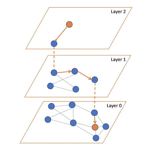
The Hierarchical Navigable Small Worlds algorithm (HNSW) is one of the most popular algorithms out there for ANN search. It was the first algorithm that the k-NN plugin supported, using a very efficient implementation from the nmslib similarity search library. It has one of the best query latency vs. recall trade-offs and doesn’t require any training. The core idea of the algorithm is to build a graph with edges connecting index vectors that are close to each other. Then, on search, this graph is partially traversed to find the approximate nearest neighbors to the query vector. To steer the traversal towards the query’s nearest neighbors, the algorithm always visits the closest candidate to the query vector next.

But which vector should the traversal start from? It could just pick a random vector, but for a large index, this might be very far from the query’s actual nearest neighbors, leading to poor results. To pick a vector that is generally close to the query vector to start from, the algorithm builds not just one graph, but a hierarchy of graphs. All vectors are added to the bottom layer, and then a random subset of those are added to the layer above, and then a subset of those are added to the layer above that, and so on.

During search, we start from a random vector in the top layer, partially traverse the graph to find (approximately) the nearest point to the query vector in that layer, and then use this vector as the starting point for our traversal of the layer below. We repeat this until we get to the bottom layer. At the bottom layer, we perform the traversal, but this time, instead of just searching for the nearest neighbor, we keep track of the k-nearest neighbors that are visited along the way.

The following figure illustrates this process (inspired from the image in original paper Efficient and robust approximate nearest neighbor search using Hierarchical Navigable Small World graphs).

You can tune three parameters for HNSW:

  • m – The maximum number of edges a vector will get in a graph. The higher this number is, the more memory the graph will consume, but the better the search approximation may be.
  • ef_search – The size of the queue of the candidate nodes to visit during traversal. When a node is visited, its neighbors are added to the queue to be visited in the future. When this queue is empty, the traversal will end. A larger value will increase search latency, but may provide better search approximation.
  • ef_construction – Very similar to ef_search. When a node is to be inserted into the graph, the algorithm will find its m edges by querying the graph with the new node as the query vector. This parameter controls the candidate queue size for this traversal. A larger value will increase index latency, but may provide a better search approximation.

For more information on HNSW, you can read through the paper Efficient and robust approximate nearest neighbor search using Hierarchical Navigable Small World graphs.

Memory consumption

Although HNSW provides very good approximate nearest neighbor search at low latencies, it can consume a large amount of memory. Each HNSW graph uses roughly 1.1 * (4 * d + 8 * m) * num_vectors bytes of memory:

  • d is the dimension of the vectors
  • m is the algorithm parameter that controls the number of connections each node will have in a layer
  • num_vectors is the number of vectors in the index

To ensure durability and availability, especially when running production workloads, OpenSearch indexes are recommended to have at least one replica shard. Therefore, the memory requirement is multiplied by (1 + number of replicas). For use cases where the data size is 1 billion vectors of 128 dimensions each and m is set to the default value of 16, the estimated amount of memory required would be:

1.1 * (4 * 128 + 8 * 16) * 1,000,000,000 * 2 = 1,408 GB.

If we increase the size of vectors to 512, for example, and the m to 100, which is recommended for vectors with high intrinsic dimensionality, some use cases can require a total memory of approximately 4 TB.

With OpenSearch, we can always horizontally scale the cluster to handle this memory requirement. However, this comes at the expense of raising infrastructure costs. For cases where scaling doesn’t make sense, options to reduce the memory footprint of the k-NN system need to be explored. Fortunately, there are algorithms that we can use to do this.

Inverted File System algorithm

Consider a different approach for approximating a nearest neighbor search: separate your index vectors into a set of buckets, then, to reduce your search time, only search through a subset of these buckets. From a high level, this is what the Inverted File System (IVF) ANN algorithm does. In OpenSearch 1.2, the k-NN plugin introduced support for the implementation of IVF by Faiss. Faiss is an open-sourced library from Meta for efficient similarity search and clustering of dense vectors.

However, if we just randomly split up our vectors into different buckets, and only search a subset of them, this will be a poor approximation. The IVF algorithm uses a more elegant approach. First, before indexing begins, it assigns each bucket a representative vector. When a vector is indexed, it gets added to the bucket that has the closest representative vector. This way, vectors that are closer to each other are placed roughly in the same or nearby buckets.

To determine what the representative vectors for the buckets are, the IVF algorithm requires a training step. In this step, k-Means clustering is run on a set of training data, and the centroids it produces become the representative vectors. The following diagram illustrates this process.

Inverted file system indexing concept

IVF has two parameters:

  • nlist – The number of buckets to create. More buckets will result in longer training times, but may improve the granularity of the search.
  • nprobes – The number of buckets to search. This parameter is fairly straightforward. The more buckets that are searched, the longer the search will take, but the better the approximation.

Memory consumption

In general, IVF requires less memory than HNSW because IVF doesn’t need to store a set of edges for each indexed vector.

We estimate that IVF will roughly require the following amount of memory:

1.1 * (((4 * dimension) * num_vectors) + (4 * nlist * dimension)) bytes

For the case explored for HNSW where there are 1,000,000,000 128-dimensional vectors with one layer of replication, an IVF algorithm with an nlist of 4096 would take roughly 1.1 * (((4 * 128) * 2,000,000,000) + (4 * 4096 * 128)) bytes = 1126 GB.

This savings does come at a cost, however, because HNSW offers a better query latency versus approximation accuracy tradeoff.

Product quantization vector compression

Although you can use HNSW and IVF to speed up nearest neighbor search, they can consume a considerable amount of memory. When we get into the billion-vector scale, we start to require thousands of GBs of memory to support their index structures. As we scale up the number of vectors or the dimension of vectors, this requirement continues to grow. Is there a way to use noticeably less space for our k-NN index?

The answer is yes! In fact, there are a lot of different ways to reduce the amount of memory vectors require. You can change your embedding model to produce smaller vectors, or you can apply techniques like Principle Component Analysis (PCA) to reduce the vector’s dimensionality. Another approach is to use quantization. The general idea of vector quantization is to map a large vector space with continuous values into a smaller space with discrete values. When a vector is mapped into a smaller space, it requires fewer bits to represent. However, this comes at a cost—when mapping to a smaller input space, some information about the vector is lost.

Product quantization (PQ) is a very popular quantization technique in the field of nearest neighbor search. It can be used together with ANN algorithms for nearest neighbor search. Along with IVF, the k-NN plugin added support for Faiss’s PQ implementation in OpenSearch 1.2.

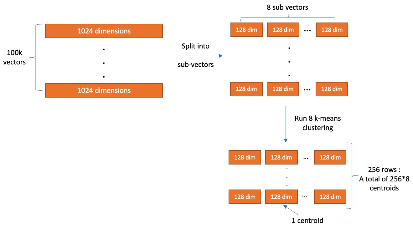
The main idea of PQ is to break up a vector into several sub-vectors and encode the sub-vectors independently with a fixed number of bits. The number of sub-vectors that the original vector is broken up into is controlled by a parameter, m, and the number of bits to encode each sub-vector with is controlled by a parameter, code_size. After encoding finishes, a vector is compressed into roughly m * code_size bits. So, assume we have a set of 100,000 1024-dimensional vectors. With m = 8 and code_size = 8, PQ breaks each vector into 8 128-dimensional sub-vectors and encode each sub-vector with 8 bits.

The values used for encoding are produced during a training step. During training, tables are created with 2code_size entries for each sub-vector partition. Next, k-Means clustering, with a k value of 2code_size, is run on the corresponding partition of sub-vectors from the training data. The centroids produced here are added as the entries to the partition’s table.

After all the tables are created, we encode a vector by replacing each sub-vector with the ID of the closest vector in the partition’s table. In the example where code_size = 8, we only need 8 bits to store an ID because there are 28 elements in the table. So, with dimension = 1024 and m = 8, the total size of one vector (assuming it uses a 32-bit floating point data type) is reduced from 4,096 bytes to roughly 8 bytes!

Product quantization encoding step

When we want to decode a vector, we can reconstruct an approximated version of it by using the stored IDs to retrieve the vectors from each partition’s table. The distance from the query vector to the reconstructed vector can then be computed and used in a nearest neighbor search. (It’s worth noting that, in practice, further optimization techniques like ADC are used to speed up this process for k-NN search).

Product quantization decoding step

Memory consumption

As we mentioned earlier, PQ will encode each vector into roughly m * code_size bits plus some overhead for each vector.

When combining it with IVF, we can estimate the index size as follows:

1.1 * ((((code_size/8) * m + overhead_per_vector) * num_vectors) + (4 * nlist * dimension) + (2 code_size * 4 * dimension) bytes

Using 1 billion vectors, dimension = 128, m = 8, code_size = 8, and nlist = 4096, we get an estimated total memory consumption of 70GB: 1.1 * ((((8 / 8) * 8 + 24) * 1,000,000,000) + (4 * 4096 * 128) + (2^8 * 4 * 128)) * 2 = 70 GB.

Running k-NN with OpenSearch

First make sure you have an OpenSearch cluster up and running. For instructions, refer to Cluster formation. For a more managed solution, you can use Amazon OpenSearch Service.

Before getting into the experiments, let’s go over how to run k-NN workloads in OpenSearch. First, we need to create an index. An index stores a set of documents in a way that they can be easily searched. For k-NN, the index’s mapping tells OpenSearch what algorithms to use and what parameters to use with them. We start by creating an index that uses HNSW as its search algorithm:

PUT my-hnsw-index
{
  "settings": {
    "index": {
      "knn": true,
      "number_of_shards": 10,
      "number_of_replicas" 1,
    }
  },
  "mappings": {
    "properties": {
      "my_vector": {
        "type": "knn_vector",
        "dimension": 4,
        "method": {
          "name": "hnsw",
          "space_type": "l2",
          "engine": "nmslib",
          "parameters": {
            "ef_construction": 128,
            "m": 24
          }
        }
      }
    }
  }
}

In the settings, we need to enable knn so that the index can be searched with the knn query type (more on this later). We also set the number of shards, and the number of replicas each shard will have. An index is made up of a collection of shards. Sharding is how OpenSearch distributes an index across multiple nodes in a cluster. For more information about shards, refer to Sizing Amazon OpenSearch Service domains.

In the mappings, we configure a field called my_vector of type knn_vector to store the vector data. We also pass nmslib as the engine to let OpenSearch know it should use nmslib’s implementation of HNSW. Additionally, we pass l2 as the space_type. The space_type determines the function used to compute the distance between two vectors. l2 refers to the Euclidean distance. OpenSearch also supports cosine similarity and the inner product distance functions.

After the index is created, we can ingest some fake data:

POST _bulk
{ "index": { "_index": "my-hnsw-index", "_id": "1" } }
{ "my_vector": [1.5, 2.5], "price": 12.2 }
{ "index": { "_index": "my-hnsw-index", "_id": "2" } }
{ "my_vector": [2.5, 3.5], "price": 7.1 }
{ "index": { "_index": "my-hnsw-index", "_id": "3" } }
{ "my_vector": [3.5, 4.5], "price": 12.9 }
{ "index": { "_index": "my-hnsw-index", "_id": "4" } }
{ "my_vector": [5.5, 6.5], "price": 1.2 }
{ "index": { "_index": "my-hnsw-index", "_id": "5" } }
{ "my_vector": [4.5, 5.5], "price": 3.7 }
{ "index": { "_index": "my-hnsw-index", "_id": "6" } }
{ "my_vector": [1.5, 5.5, 4.5, 6.4], "price": 10.3 }
{ "index": { "_index": "my-hnsw-index", "_id": "7" } }
{ "my_vector": [2.5, 3.5, 5.6, 6.7], "price": 5.5 }
{ "index": { "_index": "my-hnsw-index", "_id": "8" } }
{ "my_vector": [4.5, 5.5, 6.7, 3.7], "price": 4.4 }
{ "index": { "_index": "my-hnsw-index", "_id": "9" } }
{ "my_vector": [1.5, 5.5, 4.5, 6.4], "price": 8.9 }

After adding some documents to the index, we can search it:

GET my-hnsw-index/_search
{
  "size": 2,
  "query": {
    "knn": {
      "my_vector": {
        "vector": [2, 3, 5, 6],
        "k": 2
      }
    }
  }
}

Creating an index that uses IVF or PQ is a little bit different because these algorithms require training. Before creating the index, we need to create a model using the training API:

POST /_plugins/_knn/models/my_ivfpq_model/_train
{
  "training_index": "train-index",
  "training_field": "train-field",
  "dimension": 128,
  "description": "My model description",
  "method": {
      "name":"ivf",
      "engine":"faiss",
      "parameters":{
        "encoder":{
            "name":"pq",
            "parameters":{
                "code_size": 8,
                "m": 8
            }
        }
      }
  }
}

The training_index and training_field specify where the training data is stored. The only requirement for the training data index is that it has a knn_vector field that has the same dimension as you want your model to have. The method defines the algorithm that should be used for search.

After the training request is submitted, it will run in the background. To check if the training is complete, you can use the GET model API:

GET /_plugins/_knn/models/my_ivfpq_model/filter_path=model_id,state
{
  "model_id" : "my_ivfpq_model",
  "state" : "created"
}

After the model is created, you can create an index that uses this model:

PUT /my-hnsw-index
{
  "settings" : {
    "index.knn": true
    "number_of_shards" : 10,
    "number_of_replicas" : 1,
  },
  "mappings": {
    "properties": {
      "my_vector": {
        "type": "knn_vector",
        "model_id": "my_ivfpq_model"
      }
    }
  }
}

After the index is created, we can add documents to it and search it just like we did for HNSW.

Experiments

Let’s run a few experiments to see how these algorithms perform in practice and what tradeoffs are made. We look at an HNSW versus an IVF index using PQ. For these experiments, we’re interested in search accuracy, query latency, and memory consumption. Because these trade-offs are mainly observed at scale, we use the BIGANN dataset containing 1 billion vectors of 128 dimensions. The dataset also contains 10,000 queries of test data mapping a query to the ground truth closest 100 vectors based on the Euclidean distance.

Specifically, we compute the following search metrics:

  • Latency p99 (ms), Latency p90 (ms), Latency p50 (ms) – Query latency at various quantiles in milliseconds
  • recall@10 – The fraction of the top 10 ground truth neighbors found in the 10 results returned by the plugin
  • Native memory consumption (GB) – The amount of memory used by the plugin during querying

One thing to note is that the BIGANN dataset uses an unsigned integer as the data type. Because the knn_vector field doesn’t support unsigned integers, the data is automatically converted to floats.

To run the experiments, we complete the following steps:

  1. Ingest the dataset into the cluster using the OpenSearch Benchmarks framework (the code can be found on GitHub).
  2. When ingestion is complete, we use the warmup API to prepare the cluster for the search workload.
  3. We run the 10,000 test queries against the cluster 10 times and collect the aggregated results.

The queries return the document ID only, and not the vector, to improve performance (code for this can be found on GitHub).

Parameter selection

One tricky aspect of running experiments is selecting the parameters. There are too many different combinations of parameters to test them all. That being said, we decided to create three configurations for HNSW and IVFPQ:

  • Optimize for search latency and memory
  • Optimize for recall
  • Fall somewhere in the middle

For each optimization strategy, we chose two configurations.

For HNSW, we can tune the m, ef_construction, and ef_search parameters to achieve our desired trade-off:

  • m – Controls the maximum number of edges a node in a graph can have. Because each node has to store all of its edges, increasing this value will increase the memory footprint, but also increase the connectivity of the graph, which will improve recall.
  • ef_construction – Controls the size of the candidate queue for edges when adding a node to the graph. Increasing this value will increase the number of candidates to consider, which will increase the index latency. However, because more candidates will be considered, the quality of the graph will be better, leading to better recall during search.
  • ef_search – Similar to ef_construction, it controls the size of the candidate queue for graph traversal during search. Increasing this value will increase the search latency, but will also improve the recall.

In general, we chose configurations that gradually increased the parameters, as detailed in the following table.

Config ID Optimization Strategy m ef_construction ef_search
hnsw1 Optimize for memory and search latency 8 32 32
hnsw2 Optimize for memory and search latency 16 32 32
hnsw3 Balance between latency, memory, and recall 16 128 128
hnsw4 Balance between latency, memory, and recall 32 256 256
hnsw5 Optimize for recall 32 512 512
hnsw6 Optimize for recall 64 512 512

For IVF, we can tune two parameters:

  • nlist – Controls the granularity of the partitioning. The recommended value for this parameter is a function of the number of vectors in the index. One thing to keep in mind is that there are Faiss indexes that map to Lucene segments. There are several Lucene segments per shard and several shards per OpenSearch index. For our estimates, we assumed that there would be 100 segments per shard and 24 shards, so about 420,000 vectors per Faiss index. With this value, we estimated a good value to be 4096 and kept this constant for the experiments.
  • nprobes – Controls the number of nlist buckets we search. Higher values generally lead to improved recalls at the expense of increased search latencies.

For PQ, we can tune two parameters:

  • mControls the number of partitions to break the vector into. The larger this value is, the better the encoding will approximate the original, at the expense of raising memory consumption.
  • code_sizeControls the number of bits to encode a sub-vector with. The larger this value is, the better the encoding approximates the original, at the expense of raising memory consumption. The max value is 8, so we kept it constant at 8 for all experiments.

The following table summarizes our strategies.

Config ID Optimization Strategy nprobes m (num_sub_vectors)
ivfpq1 Optimize for memory and search latency 8 8
ivfpq2 Optimize for memory and search latency 16 8
ivfpq3 Balance between latency, memory, and recall 32 16
ivfpq4 Balance between latency, memory, and recall 64 32
ivfpq5 Optimize for recall 128 16
ivfpq6 Optimize for recall 128 32

Additionally, we need to figure out how much training data to use for IVFPQ. In general, Faiss recommends between 30,000 and 256,000 training vectors for components involving k-Means training. For our configurations, the maximum k for k-Means is 4096 from the nlist parameter. With this formula, the recommended training set size is between 122,880 and 1,048,576 vectors, so we settled on 1 million vectors. The training data comes from the index vector dataset.

Lastly, for the index configurations, we need to select the shard count. It is recommended to keep the shard size between 10–50 GBs for OpenSearch. Experimentally, we determined that for HNSW, a good number would be 64 shards and for IVFPQ, 42. Both index configurations were configured with one replica.

Cluster configuration

To run these experiments, we used Amazon OpenSearch Service using version 1.3 of OpenSearch to create the clusters. We decided to use the r5 instance family, which provides a good trade-off between memory size and cost.

The number of nodes will depend on the amount of memory that can be used for the algorithm per node and the total amount of memory required by the algorithm. Having more nodes and more memory will generally improve performance, but for these experiments, we want to minimize cost. The amount of memory available per node is computed as memory_available = (node_memory - jvm_size) * circuit_breaker_limit, with the following parameters:

  • node_memory – The total memory of the instance.
  • jvm_size – The OpenSearch JVM heap size. Set to 32 GB.
  • circuit_breaker_limit – The native memory usage threshold for the circuit breaker. Set to 0.5.

Because HNSW and IVFPQ have different memory requirements, we estimate how much memory is needed for each algorithm and determine the required number of nodes accordingly.

For HNSW, with m = 64, the total memory required using the formula from the previous sections is approximately 2,252 GB. Therefore, with r5.12xlarge (384 GB of memory), memory_available is 176 GB and the total number of nodes required is about 12, which we round up to 16 for stability purposes.

Because the IVFPQ algorithm requires less memory, we can use a smaller instance type, the r5.4xlarge instance, which has 128 GB of memory. Therefore, the memory_available for the algorithm is 48 GB. The estimated algorithm memory consumption where m = 64 is a total of 193 GB and the total number of nodes required is four, which we round up to six for stability purposes.

For both clusters, we use c5.2xlarge instance types as dedicated leader nodes. This will provide more stability for the cluster.

According to the AWS Pricing Calculator, for this particular use case, the cost per hour of the HNSW cluster is around $75 an hour, and the IVFPQ cluster costs around $11 an hour. This is important to remember when comparing the results.

Also, keep in mind that these benchmarks can be run using your custom infrastructure, using Amazon Elastic Compute Cloud (Amazon EC2), as long as the instance types and their memory size is equivalent.

Results

The following tables summarize the results from the experiments.

Test ID p50 Query latency (ms) p90 Query latency (ms) p99 Query latency (ms) Recall@10 Native memory consumption (GB)
hnsw1 9.1 11 16.9 0.84 1182
hnsw2 11 12.1 17.8 0.93 1305
hnsw3 23.1 27.1 32.2 0.99 1306
hnsw4 54.1 68.3 80.2 0.99 1555
hnsw5 83.4 100.6 114.7 0.99 1555
hnsw6 103.7 131.8 151.7 0.99 2055
Test ID p50 Query latency (ms) p90 Query latency (ms) p99 Query latency (ms) Recall@10 Native memory consumption (GB)
ivfpq1 74.9 100.5 106.4 0.17 68
ivfpq2 78.5 104.6 110.2 0.18 68
ivfpq3 87.8 107 122 0.39 83
ivfpq4 117.2 131.1 151.8 0.61 114
ivfpq5 128.3 174.1 195.7 0.40 83
ivfpq6 163 196.5 228.9 0.61 114

As you might expect, given how many more resources it uses, the HNSW cluster has lower query latencies and better recall. However, the IVFPQ indexes use significantly less memory.

For HNSW, increasing the parameters does in fact lead to better recall at the expense of latency. For IVFPQ, increasing m has the most significant impact on improving recall. Increasing nprobes improves the recall marginally, but at the expense of significant increases in latencies.

Conclusion

In this post, we covered different algorithms and techniques used to perform approximate k-NN search at scale (over 1 billion data points) within OpenSearch. As we saw in the previous benchmarks section, there isn’t one algorithm or approach that optimises for all the metrics at once. HNSW, IVF, and PQ each allow you to optimize for different metrics in your k-NN workload. When choosing the k-NN algorithm to use, first understand the requirements of your use case (How accurate does my approximate nearest neighbor search need to be? How fast should it be? What’s my budget?) and then tailor the algorithm configuration to meet them.

You can take a look at the benchmarking code base we used on GitHub. You can also get started with approximate k-NN search today following the instructions in Approximate k-NN search. If you’re looking for a managed solution for your OpenSearch cluster, check out Amazon OpenSearch Service.


About the Authors

Jack Mazanec is a software engineer working on OpenSearch plugins. His primary interests include machine learning and search engines. Outside of work, he enjoys skiing and watching sports.

Othmane Hamzaoui is a Data Scientist working at AWS. He is passionate about solving customer challenges using Machine Learning, with a focus on bridging the gap between research and business to achieve impactful outcomes. In his spare time, he enjoys running and discovering new coffee shops in the beautiful city of Paris.