Amazon QuickSight is a fast and cloud-powered business intelligence (BI) service that makes it easy to create and deliver insights to everyone in your organization without any servers or infrastructure. QuickSight dashboards can also be embedded into applications and portals to deliver insights to external stakeholders. Additionally, with Amazon QuickSight Q, end-users can simply ask questions in natural language to get machine learning (ML)-powered visual responses to their questions.
Recently, Amazon FinTech migrated all their financial reporting to QuickSight. This involved migrating complex tables and pivot tables, helping them slice and dice large datasets and deliver pixel-perfect views of their data to their stakeholders. Amazon FinTech, like all QuickSight customers, needs fast performance on very large pivot tables in order to drive adoption of their dashboards. We have specifically launched two new features focused on scaling our pivot tables with the following improvements:
Faster loading of pivot tables during expand and collapse operations
Increased field limits for rows, columns, and values
In this post, we discuss these improvements to pivot tables in QuickSight.
Blazing fast pivot tables during expand and collapse operations
Today, QuickSight pivot tables work as an infinite load. As users scroll vertically or horizontally on the visual, new queries are run to fetch additional rows and columns of data with fixed row and column configurations for every query request.
For example, in the following table, we would load all carrier/city combinations nested under Dec 7, 2014 before we can continue querying the next date. Let’s say we have more than 500 carrier/city rows for a specific date; this will take more than a single query to get to the next date. The count of queries run depends on the cardinality of the dimension used in the pivot table.
In the following example of a collapsed pivot table, since the reader doesn’t see anything beyond the flight dates, having all carrier/city rows doesn’t change what is actively displayed on the pivot table. Even though individual SQL queries can be fast, users can perceive this table to load slowly due to the sheer number of queries being fired to load the hidden (collapsed) data. Therefore, loading every single row up to the Destination City field isn’t very useful when the pivot table in the collapsed state.
Therefore, to make our pivot tables load faster, we now only fetch the data for visible fields (expanded fields) along with a small subset of values under the collapsed field. This makes sure that data fetched in every new query is used to render new values that can be displayed immediately. We have seen customers improve their load time from 2–10 times faster depending on the complexity of their dataset.
This new behavior is automatically enabled, without requiring users to do anything on their side. Please note that while we plan to support all kinds of pivot tables to use this optimization, our current rollout only includes pivot tables with only row or only column fields not sorted by any metric.
Increased field limits for pivot tables
With the ever-growing depth and granularity of data being collected, our customers asked us to increase the number of fields and data points they can display in their visuals. We have been actively listening to your needs, and just like supporting more data points in line charts, we now are increasing our field limits for pivot tables.
The value field well limits have been increased from 20 to 40, and rows and columns have been increased from 20 each to a combined limit of 40. For example, if the user has 34 fields in rows, then they can add up to 6 fields to the column field well.
This will help unblock use cases requiring increased limits such as:
Metrics reporting – Monthly and weekly business reporting often requires having dozens of metrics presented in tabular formats. With the updated limits, you can display detailed, robust financial reports in a single pivot table rather than having to split it across multiple pivot tables.
Migration from legacy BI and reporting tools – Existing reports in these legacy systems require displaying and slicing across a large number of row hierarchies, for example a cost center expense analysis.
Custom use cases – These are specific industry and organization use cases where you can add dozens of values and row fields to display additional attributes. For example, a customer 360 report sliced by different regions.
As soon as you hit the limit, you receive an error message to indicate that the limit has been reached for that field well. For more details, refer to here.
Get started and stay updated!
Learn more about our new features in our newly launched QuickSight community’s Announcement section and supercharge your dashboards with the latest features from QuickSight!
About the authors
Bhupinder Chadha is a senior product manager for Amazon QuickSight focused on visualization and front end experiences. He is passionate about BI, data visualization and low-code/no-code experiences. Prior to QuickSight he was the lead product manager for Inforiver, responsible for building a enterprise BI product from ground up. Bhupinder started his career in presales, followed by a small gig in consulting and then PM for xViz, an add on visualization product.
Igal Mizrahi is a Senior Software Engineer for AWS QuickSight Charting team. He has been part of the team for the past 3 years, and previously worked on Amazon’s mobile shopping application for 4 years.
This post is co-authored with Girish Kumar Chidananda from redBus.
redBus is one of the earliest adopters of AWS in India, and most of its services and applications are hosted on the AWS Cloud. AWS provided redBus the flexibility to scale their infrastructure rapidly while keeping costs extremely low. AWS has a comprehensive suite of services to cater to most of their needs, including providing customer support that redBus can vouch for.
In this post, we share redBus’s data platform architecture, and how various components are connected to form their data highway. We also discuss the challenges redBus faced in building dashboards for their real-time business intelligence (BI) use cases, and how they used Amazon QuickSight, a fast, easy-to-use, cloud-powered business analytics service that makes it easy for all employees within redBus to build visualizations and perform ad hoc analysis to gain business insights from their data, any time, and on any device.
About redBus
redBus is the world’s largest online bus ticketing platform built in India and serving more than 36 million happy customers around the world. Along with its bus ticketing vertical, redBus also runs a rail ticketing service called redRails and a bus and car rental service called rYde. It is part of the GO-MMT group, which is India’s leading online travel company, with an extensive brand portfolio that includes other prominent online travel brands like MakeMyTrip and Goibibo.
redBus’s data highway 1.0
redBus relies heavily on making data-driven decisions at every level, from its traveler journey tracking, forecasting demand during high traffic, identifying and addressing bottlenecks in their bus operators signup process, and more. As redBus’s business started growing in terms of the number of cities and countries they operated in and the number of bus operators and travelers using the service in each city, the amount of incoming data also increased. The need to access and analyze the data in one place required them to build their own data platform, as shown in the following diagram.
In the following sections, we look at each component in more detail.
Data ingestion sources
With the data platform 1.0, the data is ingested from various sources:
Real time – The real-time data flows from redBus mobile apps, the backend microservices, and when a passenger, bus operator, or application does any operation like booking bus tickets, searching the bus inventory, uploading a KYC document, and more
Batch mode – Scheduled jobs fetch data from multiple persistent data stores like Amazon Relational Database Service (Amazon RDS), where the OLTP data from all its applications are stored, Apache Cassandra clusters, where the bus inventory from various operators is stored, Arango DB, where the user identity graphs are stored, and more
Data cataloging
The real-time data is ingested into their self-managed Apache Nifi clusters, an open-source data platform that is used to clean, analyze, and catalog the data with its routing capabilities before sending the data to its destination.
Storage and analytics
redBus uses the following services for its storage and analytical needs:
Amazon Simple Storage Service (Amazon S3), an object storage service that provides the foundation for their data lake because of its virtually unlimited scalability and higher durability. Real-time data flows from Apache Druid and data from the data stores flow at regular intervals based on the schedules.
Apache Druid, an OLAP-style data store (data flows via Kafka Druid data loader), which computes facts and metrics against various dimensions during the data loading process.
Amazon Redshift, a cloud data warehouse service that helps you analyze exabytes of data and run complex analytical queries. redBus uses Amazon Redshift to store the processed data from Amazon S3 and the aggregated data from Apache Druid.
Querying and visualization
To make redBus as data-driven as possible, they ensured that the data is accessible to their SRE engineers, data engineers, and business analysts via a visualization layer. This layer features dashboards being served using Apache SuperSet, an open-source data visualization application, and Amazon Athena, an interactive query service to analyze data in Amazon S3 using standard SQL for ad hoc querying requirements.
The challenges
Initially, redBus handled data that was being ingested at the rate of 10 million events per day. Over time, as its business started growing, so did the data volume (from gigabytes to terabytes to petabytes), data ingestion per day (from 10 million to 320 million events), and its business intelligence dashboard needs. Soon after, they started facing challenges with their self-managed Superset’s BI capabilities, and the increased operational complexities.
Limited BI capabilities
redBus encountered the following BI limitations:
Inability to create visualizations from multiple data sources – Superset doesn’t allow creating visualizations from multiple tables within its data exploration layer. redBus data engineers had to have the tables joined beforehand at the data source level itself. In order to create a 360-degree view for redBus’s business stakeholders, it became inconvenient for data engineers to maintain multiple tables supporting the visualization layer.
No global filter for visuals in a dashboard – A global or primary filter across visuals in a dashboard is not supported in Superset. For example, consider there are visuals like Sales Wins by Region, YTD Revenue Realized by Region, Sales Pipeline by Region, and more in a dashboard, and a filter Region is added to the dashboard with values like EMEA, APAC, and US. The filter Region will only apply to one of the visuals, not the entire dashboard. However, dashboard users expected filtering across the dashboard.
Not a business-user friendly tool – Superset is highly developer centric when it comes to customization. For example, if a redBus business analyst had to customize a timed refresh that automatically re-queries every slice on a dashboard according to a pre-set value, then the analyst has to update the dashboard’s JSON metadata field. Therefore, having knowledge of JSON and its syntax is mandatory for doing any customization on the visuals or dashboard.
Increased operational cost
Although Superset is open source, which means there are no licensing costs, it also means there is more effort in maintaining all the components required for it to function as an enterprise-grade BI tool. redBus has deployed and maintained a web server (Nginx) fronted by an Application Load Balancer to do the load balancing; a metadata database server (MySQL) where Superset stores its internal information like users, slices, and dashboard definitions; an asynchronous task queue (Celery) for supporting long-running queries; a message broker (RabbitMQ); and a distributed caching server (Redis) for caching the results, charting data, and more on Amazon Elastic Compute Cloud (Amazon EC2) instances. The following diagram illustrates this architecture.
redBus’s DevOps team had to do the heavy lifting of provisioning the infrastructure, taking backups, scaling the components manually as needed, upgrading the components individually, and more. It also required a Python web developer to be around for making the configurational changes so all the components work together seamlessly. All these manual operations increased the total cost of ownership for redBus.
Journey towards QuickSight
redBus started exploring BI solutions primarily around a couple of its dashboarding requirements:
BI dashboards for business stakeholders and analysts, where the data is sourced via Amazon S3 and Amazon Redshift.
A real-time application performance monitoring (APM) dashboard to help their SRE engineers and developers identify the root cause of an issue in their microservices deployment so they can fix the issues before they affect their customer’s experience. In this case, the data is sourced via Druid.
QuickSight fit into most of redBus’s BI dashboard requirements, and in no time their data platform team started with a proof of concept (POC) for a couple of their complex dashboards. At the end of the POC, which spanned a month’s time, the team shared their findings.
First, QuickSight is rich in BI capabilities, including the following:
It’s a self-service BI solution with drag-and-drop features that could help redBus analysts comfortably use it without any coding efforts.
Visualizations from multiple data sources in a single dashboard could help redBus business stakeholders get a 360-degree view of sales, forecasting, and insights in a single pane of glass.
Cascading filters across visuals and across sheets in a dashboard are much-needed features for redBus’s BI requirements.
QuickSight offers Excel-like visuals—tables with calculations, pivot tables with cell grouping, and styling are attractive for the viewers.
The Super-fast, Parallel, In-memory Calculation Engine (SPICE) in QuickSight could help redBus scale to hundreds of thousands of users, who can all simultaneously perform fast interactive analysis across a wide variety of AWS data sources.
Off-the-shelf ML insights and forecasting at no additional cost would allow redBus’s data science team to focus on ML models besides sales forecasting and similar models.
Built-in row-level security (RLS) could allow redBus to grant filtered access for their viewers. For example, redBus has many business analysts who manage different countries. With RLS, each business analyst only sees data related to their assigned country within a single dashboard.
redBus uses OneLogin as its identity provider, which supports Security Assertion Markup Language 2.0 (SAML 2.0). With the help of identity federation and single sign-on support from QuickSight, redBus could provide a simple onboarding flow for their QuickSight users.
QuickSight offers built-in alerts and email notification capabilities.
Secondly, QuickSight is a fully managed, cloud-native, serverless BI service offering from AWS, with the following features:
redBus engineers don’t need to focus on the heavy lifting of provisioning, scaling, and maintaining their BI solution on EC2 instances.
QuickSight offers native integration with AWS services like Amazon Redshift, Amazon S3, and Athena, and other popular frameworks like Presto, Snowflake, Teradata, and more. QuickSight connects to most of the data sources that redBus already has except Apache Druid, because native integration with Druid was not available as of December 2022. For a complete list of the supported data sources, see Supported data sources.
The outcome
Considering all the rich features and lower total cost of ownership, redBus chose QuickSight for their BI dashboard requirements. With QuickSight, redBus’s data engineers have built a number of dashboards in no time to give insights from petabytes of data to business stakeholders and analysts. The redBus data highway evolved to bring business intelligence to a much wider audience in their organization, with better performance and faster time-to-value. As of November 2022, it combines QuickSight for business users and Superset for real-time APM dashboards (at the time of writing, QuickSight doesn’t offer a native connector to Druid), as shown in the following diagram.
Sales anomaly detection dashboard
Although there are many dashboards that redBus deployed to production, sales anomaly detection is one of the interesting dashboards that redBus built. It uses redBus’s proprietary sales forecasting model, which in turn is sourced by historical sales data from Amazon Redshift tables and real-time sales data from Druid tables, as shown in the following figure.
At regular intervals, the scheduled jobs feed the redBus forecasting model with real-time and historical sales data, and then the forecasted data is pushed into an Amazon Redshift table. The sales anomaly detection dashboard in QuickSight is served by the resultant Amazon Redshift table.
The following is one of the visuals from the sales anomaly detection dashboard. It’s built using a line chart representing hourly actual sales, predicted sales, and an alert threshold for a time series for a particular business cohort in redBus.
In this visual, each bar represents the number of sales anomalies triggered at a particular point in the time series.
redBus’s analysts could further drill down to the sales details and anomalies at the minute level, as shown in the following diagram. This drill-down feature comes out of the box with QuickSight.
Apart from the visuals, it has become one of viewers’ favorite dashboards at redBus due to the following notable features:
Because filtering across visuals is an out-of-the-box feature in QuickSight, a timestamp-based filter is added to the dashboard. This helps in filtering multiple visuals in the dashboard in a single click.
URL actions configured on the visuals help the viewers navigate to the context-sensitive in-house applications.
Email alerts configured on KPIs and Gauge visuals help the viewers get notifications on time.
Next steps
Apart from building new dashboards for their BI dashboard needs, redBus is taking the following next steps:
Exploring QuickSight Embedded Analytics for a couple of their application requirements to accelerate time to insights for users with in-context data visuals, interactive dashboards, and more directly within applications
Exploring QuickSight Q, which could enable their business stakeholders to ask questions in natural language and receive accurate answers with relevant visualizations that can help them gain insights from the data
Building a unified dashboarding solution using QuickSight covering all their data sources as integrations become available
Conclusion
In this post, we showed you how redBus built its data platform using various AWS services and Apache frameworks, the challenges the platform went through (especially in their BI dashboard requirements and challenges while scaling), and how they used QuickSight and lowered the total cost of ownership.
To know more about engineering at redBus, check out their medium blog posts. To learn more about what is happening in QuickSight or if you have any questions, reach out to the QuickSight Community, which is very active and offers several resources.
About the Authors
Girish Kumar Chidananda works as a Senior Engineering Manager – Data Engineering at redBus, where he has been building various data engineering applications and components for redBus for the last 5 years. Prior to starting his journey in the IT industry, he worked as a Mechanical and Control systems engineer in various organizations, and he holds an MS degree in Fluid Power Engineering from University of Bath.
Kayalvizhi Kandasamy works with digital-native companies to support their innovation. As a Senior Solutions Architect (APAC) at Amazon Web Services, she uses her experience to help people bring their ideas to life, focusing primarily on microservice architectures and cloud-native solutions using AWS services. Outside of work, she likes playing chess and is a FIDE rated chess player. She also coaches her daughters the art of playing chess, and prepares them for various chess tournaments.
AWS re:Invent is a learning conference hosted by AWS for the global cloud computing community. Re:Invent was held at the end of 2022 in Las Vegas, Nevada, from November 28 to December 2.
Amazon QuickSight powers data-driven organizations with unified business intelligence (BI) at hyperscale. This post walks you through a full recap of QuickSight at this year’s re:Invent, including key launch announcements, sessions available virtually, and additional resources for continued learning.
This press release covers five new QuickSight capabilities to help you streamline business intelligence operations, using the most popular serverless BI service built for the cloud.
Automated data preparation utilizes machine learning (ML) to infer semantic information about data and adds it to datasets as metadata about the columns (fields), making it faster for you to prepare data in order to support natural language questions.
This feature allows you to create and share highly formatted, personalized reports containing business-critical data to hundreds of thousands of end-users—without any infrastructure setup or maintenance, up-front licensing, or long-term commitments.
Keynotes
Adam Selipsky, Chief Executive Officer of Amazon Web Services
Watch Adam Selipsky, Chief Executive Officer of Amazon Web Services, as he looks at the ways that forward-thinking builders are transforming industries and even our future, powered by AWS. He highlights innovations in data, infrastructure, and more that are helping customers achieve their goals faster, take advantage of untapped potential, and create a better future with AWS.
Swami Sivasubramanian, Vice President of AWS Data and Machine Learning
Watch Swami Sivasubramanian, Vice President of AWS Data and Machine Learning, as he reveals the latest AWS innovations that can help you transform your company’s data into meaningful insights and actions for your business. In this keynote, several speakers discuss the key components of a future-proof data strategy and how to empower your organization to drive the next wave of modern invention with data. Hear from leading AWS customers who are using data to bring new experiences to life for their customers.
Leadership sessions
Unlock the value of your data with AWS analytics
Data fuels digital transformation and drives effective business decisions. To survive in an ever-changing world, organizations are turning to data to derive insights, create new experiences, and reinvent themselves so they can remain relevant today and in the future. AWS offers analytics services that allow organizations to gain faster and deeper insights from all their data. In this session, G2 Krishnamoorthy, VP of AWS Analytics, addresses the current state of analytics on AWS, covers the latest service innovations around data, and highlights customer successes with AWS analytics. Also, learn from organizations like FINRA and more who have turned to AWS for their digital transformation journey.
Reinvent how you derive value from your data with Amazon QuickSight
In this session, learn how you can use AWS-native business analytics to provide your users with ML-powered interactive dashboards, natural language query (NLQ), and embedded analytics to provide insights to users at scale, when and where they need it. Watch this session to also learn more about how Amazon uses QuickSight internally.
Breakout sessions
What’s New with Amazon QuickSight?
This session covers all of QuickSight’s newly launched capabilities, including paginated reporting in the cloud, 1 billion rows of data with SPICE, assets as code, and new Amazon QuickSight Q capabilities, including ML-powered semantic inferencing, forecasting, new question types, and more.
Differentiate your apps with Amazon QuickSight embedded analytics
Watch this session to learn how to enable new monetization opportunities and grow your business with QuickSight embedded analytics. Discover how you can differentiate your end-user experience by embedding data visualizations, dashboards, and ML-powered natural language query into your applications at scale with no infrastructure to manage. Hear from customers Guardian Life and Showpad and learn more about their QuickSight use cases.
Migrate to cloud-native business analytics with Amazon QuickSight
Legacy BI systems can hurt agile decision-making in the modern organization, with expensive licensing, outdated capabilities, and expensive infrastructure management. In this session, discover how migrating your BI to the cloud with cloud-native, fully managed business analytics capabilities from QuickSight can help you overcome these challenges. Learn how you can use QuickSight’s interactive dashboards and reporting capabilities to provide insights to every user in the organization, lowering your costs and enabling better decision-making. Watch this session to also learn more about Siemens’s QuickSight use case.
Get clarity on your data in seconds with Amazon QuickSight Q
Amazon QuickSight Q is an ML–powered natural language capability that empowers business users to ask questions about all of their data using everyday business language and get answers in seconds. Q interprets questions to understand their intent and generates an answer instantly in the form of a visual without requiring authors to create graphics, dashboards, or analyses. In this session, the QuickSight Q team provides an overview and demonstration of Q in action. Watch this session to also learn more about NASDAQ’s QuickSight use case.
Optimize your AWS cost and usage with Cloud Intelligence Dashboards
Do your engineers know how much they’re spending? Do you have insight into the details of your cost and usage on AWS? Are you taking advantage of all your cost optimization opportunities? Attend this session to learn how organizations are using the Cloud Intelligence Dashboards to start their FinOps journeys and create cost-aware cultures within their organizations. Dive deep into specific use cases and learn how you can use these insights to drive and measure your cost optimization efforts. Discover how unit economics, resource-level visibility, and periodic spend updates make it possible for FinOps practitioners, developers, and business executives to come together to make smarter decisions. Watch this session to also learn more about Dolby laboratories’ QuickSight use case.
Useful resources
QuickSight Community – Ask, answer, and learn with others in the QuickSight Community.
QuickSight YouTube Channel– Subscribe to stay up to date on the latest QuickSight workshops, getting started tutorials, and demo videos.
QuickSight DemoCentral – Experience QuickSight first-hand through interactive dashboards and demos.
QuickSight workshops – Enhance your BI skills with self-paced QuickSight workshops.
With the QuickSight re:Invent breakout session recordings and additional resources, we hope that you learn how to dive deeper into your data with QuickSight. For continued learning, check out more information and resources via our website.
About the author
Mia Heard is a product marketing manager for Amazon QuickSight, AWS’ cloud-native, fully managed BI service.
This is a guest post co-authored by Mahesh Vandi Chalil, Chief Technology Officer of BookMyShow.
BookMyShow (BMS), a leading entertainment company in India, provides an online ticketing platform for movies, plays, concerts, and sporting events. Selling up to 200 million tickets on an annual run rate basis (pre-COVID) to customers in India, Sri Lanka, Singapore, Indonesia, and the Middle East, BookMyShow also offers an online media streaming service and end-to-end management for virtual and on-ground entertainment experiences across all genres.
The pandemic gave BMS the opportunity to migrate and modernize our 15-year-old analytics solution to a modern data architecture on AWS. This architecture is modern, secure, governed, and cost-optimized architecture, with the ability to scale to petabytes. BMS migrated and modernized from on-premises and other cloud platforms to AWS in just four months. This project was run in parallel with our application migration project and achieved 90% cost savings in storage and 80% cost savings in analytics spend.
The BMS analytics platform caters to business needs for sales and marketing, finance, and business partners (e.g., cinemas and event owners), and provides application functionality for audience, personalization, pricing, and data science teams. The prior analytics solution had multiple copies of data, for a total of over 40 TB, with approximately 80 TB of data in other cloud storage. Data was stored on‑premises and in the cloud in various data stores. Growing organically, the teams had the freedom to choose their technology stack for individual projects, which led to the proliferation of various tools, technology, and practices. Individual teams for personalization, audience, data engineering, data science, and analytics used a variety of products for ingestion, data processing, and visualization.
This post discusses BMS’s migration and modernization journey, and how BMS, AWS, and AWS Partner Minfy Technologies team worked together to successfully complete the migration in four months and saving costs. The migration tenets using the AWS modern data architecture made the project a huge success.
Challenges in the prior analytics platform
Varied Technology: Multiple teams used various products, languages, and versions of software.
Larger Migration Project: Because the analytics modernization was a parallel project with application migration, planning was crucial in order to consider the changes in core applications and project timelines.
Resources: Experienced resource churn from the application migration project, and had very little documentation of current systems.
Data : Had multiple copies of data and no single source of truth; each data store provided a view for the business unit.
Ingestion Pipelines: Complex data pipelines moved data across various data stores at varied frequencies. We had multiple approaches in place to ingest data to Cloudera, via over 100 Kafka consumers from transaction systems and MQTT(Message Queue Telemetry Transport messaging protocol) for clickstreams, stored procedures, and Spark jobs. We had approximately 100 jobs for data ingestion across Spark, Alteryx, Beam, NiFi, and more.
Hadoop Clusters: Large dedicated hardware on which the Hadoop clusters were configured incurring fixed costs. On-premises Cloudera setup catered to most of the data engineering, audience, and personalization batch processing workloads. Teams had their implementation of HBase and Hive for our audience and personalization applications.
Data warehouse: The data engineering team used TiDB as their on-premises data warehouse. However, each consumer team had their own perspective of data needed for analysis. As this siloed architecture evolved, it resulted in expensive storage and operational costs to maintain these separate environments.
Analytics Database: The analytics team used data sourced from other transactional systems and denormalized data. The team had their own extract, transform, and load (ETL) pipeline, using Alteryx with a visualization tool.
Migration tenets followed which led to project success:
Prioritize by business functionality.
Apply best practices when building a modern data architecture from Day 1.
Move only required data, canonicalize the data, and store it in the most optimal format in the target. Remove data redundancy as much possible. Mark scope for optimization for the future when changes are intrusive.
Build the data architecture while keeping data formats, volumes, governance, and security in mind.
Simplify ELT and processing jobs by categorizing the jobs as rehosted, rewritten, and retired. Finalize canonical data format, transformation, enrichment, compression, and storage format as Parquet.
Rehost machine learning (ML) jobs that were critical for business.
Work backward to achieve our goals, and clear roadblocks and alter decisions to move forward.
Use serverless options as a first option and pay per use. Assess the cost and effort for rearchitecting to select the right approach. Execute a proof of concept to validate this for each component and service.
Strategies applied to succeed in this migration:
Team – We created a unified team with people from data engineering, analytics, and data science as part of the analytics migration project. Site reliability engineering (SRE) and application teams were involved when critical decisions were needed regarding data or timeline for alignment. The analytics, data engineering, and data science teams spent considerable time planning, understanding the code, and iteratively looking at the existing data sources, data pipelines, and processing jobs. AWS team with partner team from Minfy Technologies helped BMS arrive at a migration plan after a proof of concept for each of the components in data ingestion, data processing, data warehouse, ML, and analytics dashboards.
Workshops – The AWS team conducted a series of workshops and immersion days, and coached the BMS team on the technology and best practices to deploy the analytics services. The AWS team helped BMS explore the configuration and benefits of the migration approach for each scenario (data migration, data pipeline, data processing, visualization, and machine learning) via proof-of-concepts (POCs). The team captured the changes required in the existing code for migration. BMS team also got acquainted with the following AWS services:
Proof of concept – The BMS team, with help from the partner and AWS team, implemented multiple proofs of concept to validate the migration approach:
Performed batch processing of Spark jobs in Amazon EMR, in which we checked the runtime, required code changes, and cost.
Ran clickstream analysis jobs in Amazon EMR, testing the end-to-end pipeline. Team conducted proofs of concept on AWS IoT Core for MQTT protocol and streaming to Amazon S3.
Migrated ML models to Amazon SageMaker and orchestrated with Amazon MWAA.
Created sample QuickSight reports and dashboards, in which features and time to build were assessed.
Configured for key scenarios for Amazon Redshift, in which time for loading data, query performance, and cost were assessed.
Effort vs. cost analysis – Team performed the following assessments:
Compared the ingestion pipelines, the difference in data structure in each store, the basis of the current business need for the data source, the activity for preprocessing the data before migration, data migration to Amazon S3, and change data capture (CDC) from the migrated applications in AWS.
Assessed the effort to migrate approximately 200 jobs, determined which jobs were redundant or need improvement from a functional perspective, and completed a migration list for the target state. The modernization of the MQTT workflow code to serverless was time-consuming, decided to rehost on Amazon Elastic Compute Cloud (Amazon EC2) and modernization to Amazon Kinesis in to the next phase.
Reviewed over 400 reports and dashboards, prioritized development in phases, and reassessed business user needs.
AWS cloud services chosen for proposed architecture:
Data lake – We used Amazon S3 as the data lake to store the single truth of information for all raw and processed data, thereby reducing the copies of data storage and storage costs.
Ingestion – Because we had multiple sources of truth in the current architecture, we arrived at a common structure before migration to Amazon S3, and existing pipelines were modified to do preprocessing. These one-time preprocessing jobs were run in Cloudera, because the source data was on-premises, and on Amazon EMR for data in the cloud. We designed new data pipelines for ingestion from transactional systems on the AWS cloud using AWS Glue ETL.
Processing – Processing jobs were segregated based on runtime into two categories: batch and near-real time. Batch processes were further divided into transient Amazon EMR clusters with varying runtimes and Hadoop application requirements like HBase. Near-real-time jobs were provisioned in an Amazon EMR permanent cluster for clickstream analytics, and a data pipeline from transactional systems. We adopted a serverless approach using AWS Glue ETL for new data pipelines from transactional systems on the AWS cloud.
Data warehouse – We chose Amazon Redshift as our data warehouse, and planned on how the data would be distributed based on query patterns.
Visualization – We built the reports in Amazon QuickSight in phases and prioritized them based on business demand. We discussed with business users their current needs and identified the immediate reports required. We defined the phases of report and dashboard creation and built the reports in Amazon QuickSight. We plan to use embedded reports for external users in the future.
Machine learning – Custom ML models were deployed on Amazon SageMaker. Existing Airflow DAGs were migrated to Amazon MWAA.
Governance, security, and compliance – Governance with Amazon Lake Formation was adopted from Day 1. We configured the AWS Glue Data Catalog to reference data used as sources and targets. We had to comply to Payment Card Industry (PCI) guidelines because payment information was in the data lake, so we ensured the necessary security policies.
Solution overview
BMS modern data architecture
The following diagram illustrates our modern data architecture.
The architecture includes the following components:
Source systems – These include the following:
Data from transactional systems stored in MariaDB (booking and transactions).
User interaction clickstream data via Kafka consumers to DataOps MariaDB.
Members and seat allocation information from MongoDB.
SQL Server for specific offers and payment information.
Data pipeline – Spark jobs on an Amazon EMR permanent cluster process the clickstream data from Kafka clusters.
Data lake – Data from source systems was stored in their respective Amazon S3 buckets, with prefixes for optimized data querying. For Amazon S3, we followed a hierarchy to store raw, summarized, and team or service-related data in different parent folders as per the source and type of data. Lifecycle polices were added to logs and temp folders of different services as per teams’ requirements.
Data processing – Transient Amazon EMR clusters are used for processing data into a curated format for the audience, personalization, and analytics teams. Small file merger jobs merge the clickstream data to a larger file size, which saved costs for one-time queries.
Governance – AWS Lake Formation enables the usage of AWS Glue crawlers to capture the schema of data stored in the data lake and version changes in the schema. The Data Catalog and security policy in AWS Lake Formation enable access to data for roles and users in Amazon Redshift, Amazon Athena, Amazon QuickSight, and data science jobs. AWS Glue ETL jobs load the processed data to Amazon Redshift at scheduled intervals.
Queries – The analytics team used Amazon Athena to perform one-time queries raised from business teams on the data lake. Because report development is in phases, Amazon Athena was used for exporting data.
Data warehouse – Amazon Redshift was used as the data warehouse, where the reports for the sales teams, management, and third parties (i.e., theaters and events) are processed and stored for quick retrieval. Views to analyze the total sales, movie sale trends, member behavior, and payment modes are configured here. We use materialized views for denormalized tables, different schemas for metadata, and transactional and behavior data.
Reports – We used Amazon QuickSight reports for various business, marketing, and product use cases.
Machine learning – Some of the models deployed on Amazon SageMaker are as follows:
Content popularity – Decides the recommended content for users.
Live event popularity – Calculates the popularity of live entertainment events in different regions.
Trending searches – Identifies trending searches across regions.
Walkthrough
Migration execution steps
We standardized tools, services, and processes for data engineering, analytics, and data science:
Data lake
Identified the source data to be migrated from Archival DB, BigQuery, TiDB, and the analytics database.
Built a canonical data model that catered to multiple business teams and reduced the copies of data, and therefore storage and operational costs. Modified existing jobs to facilitate migration to a canonical format.
Identified the source systems, capacity required, anticipated growth, owners, and access requirements.
Ran the bulk data migration to Amazon S3 from various sources.
Ingestion
Transaction systems – Retained the existing Kafka queues and consumers.
Clickstream data – Successfully conducted a proof of concept to use AWS IoT Core for MQTT protocol. But because we needed to make changes in the application to publish to AWS IoT Core, we decided to implement it as part of mobile application modernization at a later time. We decided to rehost the MQTT server on Amazon EC2.
Processing
Listed the data pipelines relevant to business and migrated them with minimal modification.
Categorized workloads into critical jobs, redundant jobs, or jobs that can be optimized:
Spark jobs were migrated to Amazon EMR.
HBase jobs were migrated to Amazon EMR with HBase.
Metadata stored in Hive-based jobs were modified to use the AWS Glue Data Catalog.
NiFi jobs were simplified and rewritten in Spark run in Amazon EMR.
Amazon EMR clusters were configured one persistent cluster for streaming the clickstream and personalization workloads. We used multiple transient clusters for running all other Spark ETL or processing jobs. We used Spot Instances for task nodes to save costs. We optimized data storage with specific jobs to merge small files and compressed file format conversions.
AWS Glue crawlers identified new data in Amazon S3. AWS Glue ETL jobs transformed and uploaded processed data to the Amazon Redshift data warehouse.
Datawarehouse
Defined the data warehouse schema by categorizing the critical reports required by the business, keeping in mind the workload and reports required in future.
Defined the staging area for incremental data loaded into Amazon Redshift, materialized views, and tuning the queries based on usage. The transaction and primary metadata are stored in Amazon Redshift to cater to all data analysis and reporting requirements. We created materialized views and denormalized tables in Amazon Redshift to use as data sources for Amazon QuickSight dashboards and segmentation jobs, respectively.
Optimally used the Amazon Redshift cluster by loading last two years data in Amazon Redshift, and used Amazon Redshift Spectrum to query historical data through external tables. This helped balance the usage and cost of the Amazon Redshift cluster.
Visualization
Amazon QuickSight dashboards were created for the sales and marketing team in Phase 1:
Sales summary report – An executive summary dashboard to get an overview of sales across the country by region, city, movie, theatre, genre, and more.
Live entertainment – A dedicated report for live entertainment vertical events.
Coupons – A report for coupons purchased and redeemed.
BookASmile – A dashboard to analyze the data for BookASmile, a charity initiative.
Machine learning
Listed the ML workloads to be migrated based on current business needs.
Priority ML processing jobs were deployed on Amazon EMR. Models were modified to use Amazon S3 as source and target, and new APIs were exposed to use the functionality. ML models were deployed on Amazon SageMaker for movies, live event clickstream analysis, and personalization.
Existing artifacts in Airflow orchestration were migrated to Amazon MWAA.
Security
AWS Lake Formation was the foundation of the data lake, with the AWS Glue Data Catalog as the foundation for the central catalog for the data stored in Amazon S3. This provided access to the data by various functionalities, including the audience, personalization, analytics, and data science teams.
Personally identifiable information (PII) and payment data was stored in the data lake and data warehouse, so we had to comply to PCI guidelines. Encryption of data at rest and in transit was considered and configured in each service level (Amazon S3, AWS Glue Data Catalog, Amazon EMR, AWS Glue, Amazon Redshift, and QuickSight). Clear roles, responsibilities, and access permissions for different user groups and privileges were listed and configured in AWS Identity and Access Management (IAM) and individual services.
Existing single sign-on (SSO) integration with Microsoft Active Directory was used for Amazon QuickSight user access.
Automation
We used AWS CloudFormation for the creation and modification of all the core and analytics services.
AWS Step Functions was used to orchestrate Spark jobs on Amazon EMR.
Scheduled jobs were configured in AWS Glue for uploading data in Amazon Redshift based on business needs.
Monitoring of the analytics services was done using Amazon CloudWatch metrics, and right-sizing of instances and configuration was achieved. Spark job performance on Amazon EMR was analyzed using the native Spark logs and Spark user interface (UI).
Lifecycle policies were applied to the data lake to optimize the data storage costs over time.
Benefits of a modern data architecture
A modern data architecture offered us the following benefits:
Scalability – We moved from a fixed infrastructure to the minimal infrastructure required, with configuration to scale on demand. Services like Amazon EMR and Amazon Redshift enable us to do this with just a few clicks.
Agility – We use purpose-built managed services instead of reinventing the wheel. Automation and monitoring were key considerations, which enable us to make changes quickly.
Serverless – Adoption of serverless services like Amazon S3, AWS Glue, Amazon Athena, AWS Step Functions, and AWS Lambda support us when our business has sudden spikes with new movies or events launched.
Cost savings – Our storage size was reduced by 90%. Our overall spend on analytics and ML was reduced by 80%.
Conclusion
In this post, we showed you how a modern data architecture on AWS helped BMS to easily share data across organizational boundaries. This allowed BMS to make decisions with speed and agility at scale; ensure compliance via unified data access, security, and governance; and to scale systems at a low cost without compromising performance. Working with the AWS and Minfy Technologies teams helped BMS choose the correct technology services and complete the migration in four months. BMS achieved the scalability and cost-optimization goals with this updated architecture, which has set the stage for innovation using graph databases and enhanced our ML projects to improve customer experience.
About the Authors
Mahesh Vandi Chalil is Chief Technology Officer at BookMyShow, India’s leading entertainment destination. Mahesh has over two decades of global experience, passionate about building scalable products that delight customers while keeping innovation as the top goal motivating his team to constantly aspire for these. Mahesh invests his energies in creating and nurturing the next generation of technology leaders and entrepreneurs, both within the organization and outside of it. A proud husband and father of two daughters and plays cricket during his leisure time.
Priya Jathar is a Solutions Architect working in Digital Native Business segment at AWS. She has more two decades of IT experience, with expertise in Application Development, Database, and Analytics. She is a builder who enjoys innovating with new technologies to achieve business goals. Currently helping customers Migrate, Modernise, and Innovate in Cloud. In her free time she likes to paint, and hone her gardening and cooking skills.
Vatsal Shah is a Senior Solutions Architect at AWS based out of Mumbai, India. He has more than nine years of industry experience, including leadership roles in product engineering, SRE, and cloud architecture. He currently focuses on enabling large startups to streamline their cloud operations and help them scale on the cloud. He also specializes in AI and Machine Learning use cases.
Amazon Macie is a fully managed data security service that uses machine learning and pattern matching to help you discover and protect sensitive data in Amazon Simple Storage Service (Amazon S3). With Macie, you can analyze objects in your S3 buckets to detect occurrences of sensitive data, such as personally identifiable information (PII), financial information, personal health information, and access credentials.
In this post, we walk you through a solution to gain comprehensive and organization-wide visibility into which types of sensitive data are present in your S3 storage, where the data is located, and how much is present. Once enabled, Macie automatically starts discovering sensitive data in your S3 storage and builds a sensitive data profile for each bucket. The profiles are organized in a visual, interactive data map, and you can use the data map to run targeted sensitive data discovery jobs. Both automated data discovery and targeted jobs produce rich, detailed sensitive data discovery results. This solution uses Amazon Athena and Amazon QuickSight to deep-dive on the Macie results, and to help you analyze, visualize, and report on sensitive data discovered by Macie, even when the data is distributed across millions of objects, thousands of S3 buckets, and thousands of AWS accounts. Athena is an interactive query service that makes it simpler to analyze data directly in Amazon S3 using standard SQL. QuickSight is a cloud-scale business intelligence tool that connects to multiple data sources, including Athena databases and tables.
This solution is relevant to data security, data governance, and security operations engineering teams.
The challenge: how to summarize sensitive data discovered in your growing S3 storage
Macie issues findings when an object is found to contain sensitive data. In addition to findings, Macie keeps a record of each S3 object analyzed in a bucket of your choice for long-term storage. These records are known as sensitive data discovery results, and they include additional context about your data in Amazon S3. Due to the large size of the results file, Macie exports the sensitive data discovery results to an S3 bucket, so you need to take additional steps to query and visualize the results. We discuss the differences between findings and results in more detail later in this post.
With the increasing number of data privacy guidelines and compliance mandates, customers need to scale their monitoring to encompass thousands of S3 buckets across their organization. The growing volume of data to assess, and the growing list of findings from discovery jobs, can make it difficult to review and remediate issues in a timely manner. In addition to viewing individual findings for specific objects, customers need a way to comprehensively view, summarize, and monitor sensitive data discovered across their S3 buckets.
To illustrate this point, we ran a Macie sensitive data discovery job on a dataset created by AWS. The dataset contains about 7,500 files that have sensitive information, and Macie generated a finding for each sensitive file analyzed, as shown in Figure 1.
Figure 1: Macie findings from the dataset
Your security team could spend days, if not months, analyzing these individual findings manually. Instead, we outline how you can use Athena and QuickSight to query and visualize the Macie sensitive data discovery results to understand your data security posture.
The additional information in the sensitive data discovery results will help you gain comprehensive visibility into your data security posture. With this visibility, you can answer questions such as the following:
What are the top 5 most commonly occurring sensitive data types?
Which AWS accounts have the most findings?
How many S3 buckets are affected by each of the sensitive data types?
Your security team can write their own customized queries to answer questions such as the following:
Is there sensitive data in AWS accounts that are used for development purposes?
Is sensitive data present in S3 buckets that previously did not contain sensitive information?
Was there a change in configuration for S3 buckets containing the greatest amount of sensitive data?
Findings provide a report of potential policy violations with an S3 bucket, or the presence of sensitive data in a specific S3 object. Each finding provides a severity rating, information about the affected resource, and additional details, such as when Macie found the issue. Findings are published to the Macie console, AWS Security Hub, and Amazon EventBridge.
In contrast, results are a collection of records for each S3 object that a Macie job analyzed. These records contain information about objects that do and do not contain sensitive data, including up to 1,000 occurrences of each sensitive data type that Macie found in a given object, and whether Macie was unable to analyze an object because of issues such as permissions settings or use of an unsupported format. If an object contains sensitive data, the results record includes detailed information that isn’t available in the finding for the object.
One of the key benefits of querying results is to uncover gaps in your data protection initiatives—these gaps can occur when data in certain buckets can’t be analyzed because Macie was denied access to those buckets, or was unable to decrypt specific objects. The following table maps some of the key differences between findings and results.
Findings
Results
Enabled by default
Yes
No
Location of published results
Macie console, Security Hub, and EventBridge
S3 bucket
Details of S3 objects that couldn’t be scanned
No
Yes
Details of S3 objects in which no sensitive data was found
No
Yes
Identification of files inside compressed archives that contain sensitive data
No
Yes
Number of occurrences reported per object
Up to 15
Up to 1,000
Retention period
90 days in Macie console
Defined by customer
Architecture
As shown in Figure 2, you can build out the solution in three steps:
Enable the results and publish them to an S3 bucket
Build out the Athena table to query the results by using SQL
Visualize the results with QuickSight
Figure 2: Architecture diagram showing the flow of the solution
Prerequisites
To implement the solution in this blog post, you must first complete the following prerequisites:
To follow along with the examples in this post, download the sample dataset. The dataset is a single .ZIP file that contains three directories (fk, rt, and mkro). For this post, we used three accounts in our organization, created an S3 bucket in each of them, and then copied each directory to an individual bucket, as shown in Figure 3.
Figure 3: Sample data loaded into three different AWS accounts
Note: All data in this blog post has been artificially created by AWS for demonstration purposes and has not been collected from any individual person. Similarly, such data does not, nor is it intended, to relate back to any individual person.
Step 1: Enable the results and publish them to an S3 bucket
Publication of the discovery results to Amazon S3 is not enabled by default. The setup requires that you specify an S3 bucket to store the results (we also refer to this as the discovery results bucket), and use an AWS Key Management Service (AWS KMS) key to encrypt the bucket.
If you are analyzing data across multiple accounts in your organization, then you need to enable the results in your delegated Macie administrator account. You do not need to enable results in individual member accounts. However, if you’re running Macie jobs in a standalone account, then you should enable the Macie results directly in that account.
Select the AWS Region from the upper right of the page.
From the left navigation pane, select Discovery results.
Select Configure now.
Select Create Bucket, and enter a unique bucket name. This will be the discovery results bucket name. Make note of this name because you will use it when you configure the Athena tables later in this post.
Under Encryption settings, select Create new key. This takes you to the AWS KMS console in a new browser tab.
In the AWS KMS console, do the following:
For Key type, choose symmetric, and for Key usage, choose Encrypt and Decrypt.
Enter a meaningful key alias (for example, macie-results-key) and description.
(Optional) For simplicity, set your current user or role as the Key Administrator.
Set your current user/role as a user of this key in the key usage permissions step. This will give you the right permissions to run the Athena queries later.
From the AWS KMS Key dropdown, select the new key.
To view KMS key policy statements that were automatically generated for your specific key, account, and Region, select View Policy. Copy these statements in their entirety to your clipboard.
Navigate back to the browser tab with the AWS KMS console and then do the following:
Select Customer managed keys.
Choose the KMS key that you created, choose Switch to policy view, and under Key policy, select Edit.
In the key policy, paste the statements that you copied. When you add the statements, do not delete any existing statements and make sure that the syntax is valid. Policies are in JSON format.
Review the inputs in the Settings page for Discovery results and then choose Save. Macie will perform a check to make sure that it has the right access to the KMS key, and then it will create a new S3 bucket with the required permissions.
If you haven’t run a Macie discovery job in the last 90 days, you will need to run a new discovery job to publish the results to the bucket.
In this step, you created a new S3 bucket and KMS key that you are using only for Macie. For instructions on how to enable and configure the results using existing resources, see Storing and retaining sensitive data discovery results with Amazon Macie. Make sure to review Macie pricing details before creating and running a sensitive data discovery job.
Step 2: Build out the Athena table to query the results using SQL
Now that you have enabled the discovery results, Macie will begin publishing them into your discovery results bucket in the form of jsonl.gz files. Depending on the amount of data, there could be thousands of individual files, with each file containing multiple records. To identify the top five most commonly occurring sensitive data types in your organization, you would need to query all of these files together.
In this step, you will configure Athena so that it can query the results using SQL syntax. Before you can run an Athena query, you must specify a query result bucket location in Amazon S3. This is different from the Macie discovery results bucket that you created in the previous step.
If you haven’t set up Athena previously, we recommend that you create a separate S3 bucket, and specify a query result location using the Athena console. After you’ve set up the query result location, you can configure Athena.
To create a new Athena database and table for the Macie results
Open the Athena console, and in the query editor, enter the following data definition language (DDL) statement. In the context of SQL, a DDL statement is a syntax for creating and modifying database objects, such as tables. For this example, we named our database macie_results.
CREATE DATABASE macie_results;
After running this step, you’ll see a new database in the Database dropdown. Make sure that the new macie_results database is selected for the next queries.
Figure 4: Create database in the Athena console
Create a table in the database by using the following DDL statement. Make sure to replace <RESULTS-BUCKET-NAME> with the name of the discovery results bucket that you created previously.
CREATE EXTERNAL TABLE maciedetail_all_jobs(
	accountid string,
	category string,
	classificationdetails struct<jobArn:string,result:struct<status:struct<code:string,reason:string>,sizeClassified:string,mimeType:string,sensitiveData:array<struct<category:string,totalCount:string,detections:array<struct<type:string,count:string,occurrences:struct<lineRanges:array<struct<start:string,`end`:string,`startColumn`:string>>,pages:array<struct<pageNumber:string>>,records:array<struct<recordIndex:string,jsonPath:string>>,cells:array<struct<row:string,`column`:string,`columnName`:string,cellReference:string>>>>>>>,customDataIdentifiers:struct<totalCount:string,detections:array<struct<arn:string,name:string,count:string,occurrences:struct<lineRanges:array<struct<start:string,`end`:string,`startColumn`:string>>,pages:array<string>,records:array<string>,cells:array<string>>>>>>,detailedResultsLocation:string,jobId:string>,
	createdat string,
	description string,
	id string,
	partition string,
	region string,
	resourcesaffected struct<s3Bucket:struct<arn:string,name:string,createdAt:string,owner:struct<displayName:string,id:string>,tags:array<string>,defaultServerSideEncryption:struct<encryptionType:string,kmsMasterKeyId:string>,publicAccess:struct<permissionConfiguration:struct<bucketLevelPermissions:struct<accessControlList:struct<allowsPublicReadAccess:boolean,allowsPublicWriteAccess:boolean>,bucketPolicy:struct<allowsPublicReadAccess:boolean,allowsPublicWriteAccess:boolean>,blockPublicAccess:struct<ignorePublicAcls:boolean,restrictPublicBuckets:boolean,blockPublicAcls:boolean,blockPublicPolicy:boolean>>,accountLevelPermissions:struct<blockPublicAccess:struct<ignorePublicAcls:boolean,restrictPublicBuckets:boolean,blockPublicAcls:boolean,blockPublicPolicy:boolean>>>,effectivePermission:string>>,s3Object:struct<bucketArn:string,key:string,path:string,extension:string,lastModified:string,eTag:string,serverSideEncryption:struct<encryptionType:string,kmsMasterKeyId:string>,size:string,storageClass:string,tags:array<string>,embeddedFileDetails:struct<filePath:string,fileExtension:string,fileSize:string,fileLastModified:string>,publicAccess:boolean>>,
	schemaversion string,
	severity struct<description:string,score:int>,
	title string,
	type string,
	updatedat string)
ROW FORMAT SERDE
	'org.openx.data.jsonserde.JsonSerDe'
WITH SERDEPROPERTIES (
	'paths'='accountId,category,classificationDetails,createdAt,description,id,partition,region,resourcesAffected,schemaVersion,severity,title,type,updatedAt')
STORED AS INPUTFORMAT
	'org.apache.hadoop.mapred.TextInputFormat'
OUTPUTFORMAT
	'org.apache.hadoop.hive.ql.io.HiveIgnoreKeyTextOutputFormat'
LOCATION
	's3://<RESULTS-BUCKET-NAME>/AWSLogs/'
After you complete this step, you will see a new table named maciedetail_all_jobs in the Tables section of the query editor.
Query the results to start gaining insights. For example, to identify the top five most common sensitive data types, run the following query:
select sensitive_data.category,
	detections_data.type,
	sum(cast(detections_data.count as INT)) total_detections
from maciedetail_all_jobs,
	unnest(classificationdetails.result.sensitiveData) as t(sensitive_data),
	unnest(sensitive_data.detections) as t(detections_data)
where classificationdetails.result.sensitiveData is not null
and resourcesaffected.s3object.embeddedfiledetails is null
group by sensitive_data.category, detections_data.type
order by total_detections desc
LIMIT 5
Running this query on the sample dataset gives the following output.
Figure 5: Results of a query showing the five most common sensitive data types in the dataset
(Optional) The previous query ran on all of the results available for Macie. You can further query which accounts have the greatest amount of sensitive data detected.
select accountid,
	sum(cast(detections_data.count as INT)) total_detections
from maciedetail_all_jobs,
	unnest(classificationdetails.result.sensitiveData) as t(sensitive_data),
	unnest(sensitive_data.detections) as t(detections_data)
where classificationdetails.result.sensitiveData is not null
and resourcesaffected.s3object.embeddedfiledetails is null
group by accountid
order by total_detections desc
To test this query, we distributed the synthetic dataset across three member accounts in our organization, ran the query, and received the following output. If you enable Macie in just a single account, then you will only receive results for that one account.
Figure 6: Query results for total number of sensitive data detections across all accounts in an organization
In the previous step, you used Athena to query your Macie discovery results. Although the queries were powerful, they only produced tabular data as their output. In this step, you will use QuickSight to visualize the results of your Macie jobs.
Before creating the visualizations, you first need to grant QuickSight the right permissions to access Athena, the results bucket, and the KMS key that you used to encrypt the results.
Paste the following statement in the key policy. When you add the statement, do not delete any existing statements, and make sure that the syntax is valid. Replace <QUICKSIGHT_SERVICE_ROLE_ARN> and <KMS_KEY_ARN> with your own information. Policies are in JSON format.
	{ "Sid": "Allow Quicksight Service Role to use the key",
		"Effect": "Allow",
		"Principal": {
			"AWS": <QUICKSIGHT_SERVICE_ROLE_ARN>
		},
		"Action": "kms:Decrypt",
		"Resource": <KMS_KEY_ARN>
	}
To allow QuickSight access to Athena and the discovery results S3 bucket
In QuickSight, in the upper right, choose your user icon to open the profile menu, and choose US East (N.Virginia). You can only modify permissions in this Region.
In the upper right, open the profile menu again, and select Manage QuickSight.
Select Security & permissions.
Under QuickSight access to AWS services, choose Manage.
Make sure that the S3 checkbox is selected, click on Select S3 buckets, and then do the following:
Choose the discovery results bucket.
You do not need to check the box under Write permissions for Athena workgroup. The write permissions are not required for this post.
Select Finish.
Make sure that the Amazon Athena checkbox is selected.
Review the selections and be careful that you don’t inadvertently disable AWS services and resources that other users might be using.
Select Save.
In QuickSight, in the upper right, open the profile menu, and choose the Region where your results bucket is located.
Now that you’ve granted QuickSight the right permissions, you can begin creating visualizations.
To create a new dataset referencing the Athena table
On the QuickSight start page, choose Datasets.
On the Datasets page, choose New dataset.
From the list of data sources, select Athena.
Enter a meaningful name for the data source (for example, macie_datasource) and choose Create data source.
Select the database that you created in Athena (for example, macie_results).
Select the table that you created in Athena (for example, maciedetail_all_jobs), and choose Select.
You can either import the data into SPICE or query the data directly. We recommend that you use SPICE for improved performance, but the visualizations will still work if you query the data directly.
To create an analysis using the data as-is, choose Visualize.
You can then visualize the Macie results in the QuickSight console. The following example shows a delegated Macie administrator account that is running a visualization, with account IDs on the y axis and the count of affected resources on the x axis.
Figure 7: Visualize query results to identify total number of sensitive data detections across accounts in an organization
You can also visualize the aggregated data in QuickSight. For example, you can view the number of findings for each sensitive data category in each S3 bucket. The Athena table doesn’t provide aggregated data necessary for visualization. Instead, you need to query the table and then visualize the output of the query.
To query the table and visualize the output in QuickSight
On the Amazon QuickSight start page, choose Datasets.
On the Datasets page, choose New dataset.
Select the data source that you created in Athena (for example, macie_datasource) and then choose Create Dataset.
Select the database that you created in Athena (for example, macie_results).
Choose Use Custom SQL, enter the following query below, and choose Confirm Query.
	select resourcesaffected.s3bucket.name as bucket_name,
		sensitive_data.category,
		detections_data.type,
		sum(cast(detections_data.count as INT)) total_detections
	from macie_results.maciedetail_all_jobs,
		unnest(classificationdetails.result.sensitiveData) as t(sensitive_data),unnest(sensitive_data.detections) as t(detections_data)
where classificationdetails.result.sensitiveData is not null
and resourcesaffected.s3object.embeddedfiledetails is null
group by resourcesaffected.s3bucket.name, sensitive_data.category, detections_data.type
order by total_detections desc
You can either import the data into SPICE or query the data directly.
To create an analysis using the data as-is, choose Visualize.
Now you can visualize the output of the query that aggregates data across your S3 buckets. For example, we used the name of the S3 bucket to group the results, and then we created a donut chart of the output, as shown in Figure 6.
Figure 8: Visualize query results for total number of sensitive data detections across each S3 bucket in an organization
From the visualizations, we can identify which buckets or accounts in our organizations contain the most sensitive data, for further action. Visualizations can also act as a dashboard to track remediation.
You can replicate the preceding steps by using the sample queries from the amazon-macie-results-analytics GitHub repo to view data that is aggregated across S3 buckets, AWS accounts, or individual Macie jobs. Using these queries with the results of your Macie results will help you get started with tracking the security posture of your data in Amazon S3.
Conclusion
In this post, you learned how to enable sensitive data discovery results for Macie, query those results with Athena, and visualize the results in QuickSight.
Because Macie sensitive data discovery results provide more granular data than the findings, you can pursue a more comprehensive incident response when sensitive data is discovered. The sample queries in this post provide answers to some generic questions that you might have. After you become familiar with the structure, you can run other interesting queries on the data.
We hope that you can use this solution to write your own queries to gain further insights into sensitive data discovered in S3 buckets, according to the business needs and regulatory requirements of your organization. You can consider using this solution to better understand and identify data security risks that need immediate attention. For example, you can use this solution to answer questions such as the following:
Is financial information present in an AWS account where it shouldn’t be?
Are S3 buckets that contain PII properly hardened with access controls and encryption?
You can also use this solution to understand gaps in your data security initiatives by tracking files that Macie couldn’t analyze due to encryption or permission issues. To further expand your knowledge of Macie capabilities and features, see the following resources:
If you have feedback about this post, submit comments in the Comments section below. If you have questions about this post, start a new thread on Amazon Macie re:Post.
Want more AWS Security news? Follow us on Twitter.
This is a guest post by Jeremy Bristow, Head of Product at Green Flag.
In the US, there’s a saying: “Sooner or later, you’ll break down and call Triple A.” In the UK, that same saying might be “Sooner or later, you’ll break down and call Green Flag.”
Green Flag has been assisting stranded motorists all over Europe for more than 50 years. Having started in the UK in 1971, with the first office located above a fish and chip shop, we have built an expansive network of automobile service providers to assist customers. With that network in place, Green Flag customers need only make a single phone call, or request service via the Green Flag app, to quickly contact a local repair garage, no matter where they’ve broken down.
Green Flag’s commitment to providing world-class service to its customers has consistently earned a Net Promoter Score (NPS) of over 70. We were also recently rated as the top breakdown provider in the H1 2022 UK Customer Satisfaction Index report, which is a national benchmark of customer satisfaction covering 13 sectors and based on 45,000 customer responses.
Unlike most breakdown providers in the UK, Green Flag doesn’t currently own a large fleet of trucks to provide roadside assistance to our 3 million plus customers. Our established network of over 200 locally operated businesses provides in-depth knowledge and expertise related to their specific areas. Our overall mission is simple: “Make motoring stress-free, safe, and simple, for every driver.”
Tech transformation to democratize data
Over the past 4 years, Green Flag has been undertaking a technology transformation with the end goal of enabling data democratization and faster data-driven decisions. This has been a massive undertaking, requiring the business to replace our entire systems architecture, which we’ve done while remaining open 24/7, 365 days a year, maintaining our industry-leading customer service standards and growing the business. Building the plane while flying it is an apt analogy, but it felt more like performing open-heart surgery while running a marathon.
Early on during our tech transformation, we made the decision to develop natively with AWS, using our in-house development team. When it came time to decide on a new business intelligence (BI) tool, it was an easy decision to switch to Amazon QuickSight.
In this post, we discuss what influenced the decision to implement QuickSight and why doing so has made a significant impact on our efficiency and agility.
Changing the game with self-serve insights
Prior to embarking on this transformation, technology had consistently been a blocker to us being able to quickly serve our customers. Our old stack was slow, hard to change, and consistently prevented us from gaining valuable and timely insights from our datasets. We were data rich, but insight poor. It was clear that the status quo was not compatible with our ambitions to grow and trade in an increasingly digital world. We needed a BI tool to bring new and meaningful insights to our data, which would help us leverage our new technologies to deliver meaningful business change.
Although going with QuickSight was an easy decision, we considered the following factors to ensure our needs would be met:
Alignment to AWS architecture – We didn’t want to invest time and development resources into complicated implementations—we wanted a seamless integration that would cause no headaches.
Ease of use – We needed an intuitive, user-friendly interface that would make it easy for any user, no matter their tech background or level of expertise in pulling data insights.
Cost – Affordability is always a concern. With AWS, we can monitor daily usage and the associated costs via our console, so there were never any surprises or hidden costs post-implementation.
Although these considerations were all top of mind, the primary driver for switching to QuickSight is rooted in the data democratization goal within our tech transformation initiative. Providing self-serve access to data and insights to everyone, no matter their tech background, has been a game changer. With QuickSight, we can now present data and insights in a meaningful, easy-to-understand format via near-real-time embedded dashboards that anyone from any tech background can easily build.
Evolving our data culture with QuickSight
Because all employees are now empowered to make data-driven decisions, our data culture has begun to evolve. Having consistent, accurate dashboards that access standardized datasets brings with it a new level of confidence in decision-making. We’re no longer wasting time on discussions about data sources or the risks of inaccuracy. QuickSight and the data governance processes we have built around its use have shifted the discussion to focus on the insights, what they tell us, and what our next steps should be.
The following screenshot shows one of Green Flag’s custom-built dashboards.
Additionally, because QuickSight is so easy to use that self-service requires minimal training and no specialized skills, our data experts can now shift from responding to constant requests for information to focusing on more valuable projects that require their technical depth and expertise. We can now work more efficiently, producing actionable insights that have never before been available, at a pace that enables us to make better decisions, faster.
Mapping our next analytics adventure
The next features that the Green Flag team plan to test and then roll out is Amazon QuickSight Q, which should allow both our data teams and business users to have a more frictionless experience with our data. The feature should enable users to interrogate complex data using simple conversational questions as if they were talking to a colleague, producing results that are then customizable. This will further empower our self-serve strategy by enabling non-technical experts to pose business questions rather than rely on technical expertise and experience.
To learn more about how you can embed customized data visuals, interactive dashboards, and natural language querying into any application, visit Amazon QuickSight Embedded.
About the Author
Jeremy “Jez” Bristow is Head of Product at Green Flag. He has been working at Green Flag, part of Direct Line Group, for over 4 years and has been co-responsible for delivering the digital transformation programme within Green Flag. They have built a cloud-based ecosystem of micro-services supported by a data platform within AWS to enable the delivery of better customer outcomes to grow their business.
Convoy is the leading digital freight network in the United States. We move millions of truckloads around the country through our connected network of carriers, saving money for shippers, increasing earnings for drivers, and eliminating carbon waste for our planet. In 2015, Convoy started a movement toward efficient freight. We build technology to find smarter ways to connect shippers with carriers while solving some of the toughest problems that result in waste in the freight industry.
As a digital freight network, Convoy uses machine learning and automation to efficiently connect shippers and carriers. As our marketplace grows, it creates a flywheel effect that benefits both sides. As more shippers join the network, drivers have better options, fewer empty miles, and fewer wasted hours, allowing them to earn more per day. As more carriers join the network, capacity increases and shippers see lower costs and higher service quality. Convoy is on a mission to transport the world with endless capacity and zero waste.
Our digital freight network collects thousands of disparate data points and intelligently connects the dots to provide transparent visibility into freight operations. By providing transparency and insights into every step of the shipment lifecycle, shippers benefit from lower costs, reduced waste, and higher carrier loyalty. To surface these insights to customers inside our product, we needed a business intelligence (BI) tool that could not only handle our volume of data, but could provide at-a-glance insights through a user-friendly interface, empowering our customers to make data-driven decisions, and taking the guesswork out of resolving unexpected issues.
After reviewing our options and evaluating which would best meet our needs, we turned to Amazon QuickSight.
In this post, we discuss how QuickSight is helping us serve our customers with the insights they need, and why we consider this business decision a win for Convoy.
From disparate data points to at-a-glance insights
Our vast network of small carriers and owner-operators, totaling more than 400,000 trucks nationwide, provides meaningful data points through the Convoy app. We require carriers to use our app when hauling loads—this is how we provide GPS tracking on 95% of live loads and 100% of drop loads. It’s also how we collect robust data around dwell times, detention costs, and more. To date, we’ve captured more than 2.7 million facility reviews in the Convoy app.
We chose QuickSight because we needed ease in development. We wanted to be able to quickly build dashboards and get them in the hands of our customers. Because this is an externally facing tool, we had data privacy and governance requirements to consider as well. Especially important was that we needed granularity in row-level security. QuickSight provided what we needed out of the box, whereas the other BI platforms we considered did not. Additionally, QuickSight’s pricing would allow us to scale the platform as our user base continues to grow.
Connecting the dots with data
The challenges facing our customers are as varied as the landscapes our carriers travel through every day. From managing delays due to weather, traffic, and unpredictable load times on the carrier’s end, to lacking freight visibility and root causes of operational issues and inaccuracies in manual reporting on the shipper’s end, there is no shortage of opportunities to improve the status quo.
The following screenshot shows performance metrics, like dwell time and incidentals per shipment, plus breakouts that show incidental types and categories for each facility.
Where we strive to meet the needs of both shippers and carriers, we’re in a unique position to connect the dots to identify gaps on one end that have corresponding inputs on the other. The challenges shippers face are often driven by pricing, complexity, and reliability of transporting goods. For carriers, their challenges are more centered on earning predictable and consistent income with the least amount of time and effort invested in finding loads, building schedules, and adjusting to delays. Our customers have sophisticated internal analytics programs, but highly granular data or synthesized data from their vendors is rare. Finding ways to develop metrics and benchmarks for specific business entities (lanes, regions, facilities, and so on) meant we would need to learn and update our products quickly. QuickSight allows us to do that.
With so many data points and opportunities to turn them into key insights, the dashboards and visualizations QuickSight provides makes spotting trends and taking proactive measures to get ahead of minor issues before they become major problems easier than ever.
When reviewing our BI options, the following factors were front and center in our decision to go with QuickSight:
Pace of development – We wanted to deliver insights to our customers quickly. The seamless integration of QuickSight with other AWS services had our dashboards up and running in no time.
Secure access to data – With row-level authorization, QuickSight gives us the flexibility we need, along with the peace of mind knowing the data is secure.
Scalable cost model – The QuickSight pricing model suits our needs, allowing us to scale based on usage.
When we first piloted our external insights product, we built a prototype with our previously used BI tool. Building future iterations with this same tool wasn’t feasible because it lacked functionality in several key areas. We needed to be able to join data from multiple sources, drill down into layers of data, and customize data based on the user accessing the information. In addition, because we were self-hosting, the overhead of scaling our footprint was going to be high. We did consider other solutions, but QuickSight was best able to offer all the features we needed, at the best price.
Visibility improves efficiency
With QuickSight, we were able to build an external-facing product for our shipper customers, helping them gain visibility into the health of their supply chain, which could then provide insights to make things run more efficiently.
The following screenshot shows incidentals, broken out by spend, type or category, and more.
With a visualization of how incidental costs break down, for example, they can see the cost of having a truck unloaded at a facility, the cost of canceling loads on a driver, the cost of having travers waiting at a facility, and more. With that visibility, our shipper customers can now begin to address systemic issues that can save them money, such as improving scheduling to reduce driver wait times.
The following screenshot shows a visualization on carrier feedback, which shippers could use to make improvements that provide a faster, smoother experience.
Future plans with partnering team expansions
They say that imitation is the purest form of flattery. Although that phrase is often used in the context of competitors who develop products and services that are suspiciously similar to an existing product or service, it can also apply to when good ideas are duplicated within an organization. That’s the case for us, in that our QuickSight adoption has drawn the attention and curiosity of partnering teams, who have reached out to us to understand our implementation specifics and the successes we’ve seen as a result.
We’re very happy with our QuickSight Embedded experience and look forward to continuing to iterate and expand its use for additional customer profiles and use cases.
To learn more about how you can embed customized data visuals, interactive dashboards, and natural language querying into any application, visit Amazon QuickSight Embedded.
About the Author
Dorothy Li is Convoy’s CTO, overseeing Convoy’s Product and Engineering group and technology strategy, shaping and scaling the company’s innovation and industry-defining technology platforms. Prior to Convoy, Dorothy held leadership roles at Amazon, most recently as Vice President of BI and Analytics at AWS. During her more than 20 years at Amazon, Dorothy helped build out Amazon’s ecommerce platform and also led and collaborated on products that had visibly impacted customers around the world – from the initial launch of Amazon Prime, to Kindle, and at AWS where she focused on data analytics and BI. Dorothy received her Bachelor of Science at Brigham Young University and studies at Shanghai International Studies University.
Amazon Identity Services is responsible for the way Amazon customers—buyers, sellers, developers—identify themselves on Amazon. Our team also manages customers’ core account information, such as names and delivery addresses. Our mission is to deliver the most intuitive, convenient, and secure authentication experience. We’re in charge of account security for Amazon, worldwide, on all device surfaces.
Identity systems make millions of security decisions per second. We ingest datasets at a large scale—processing 9 TB per hour—and produce analytical datasets that grow by billions of rows per hour. Our core business metrics within the Amazon Identity Services team are built on top of these datasets, which we use for leadership meetings, product launch decisions, metric movement investigations, and discovering new innovation opportunities to simplify security experiences for our customers.
In this post, we discuss how we use Amazon QuickSight to empower partners with self-serve data discovery.
Inaccessible insights block data-driven decisions
The sheer volume of our datasets made gathering insights a slow process. Not only that, but datasets weren’t accessible to a wide audience outside our team, such as partners, program managers, product managers, and so on. As a result, Business Intelligence Engineers (BIEs) spent a lot of time writing ad hoc queries, which then took a long time to run. When the insights were ready, BIEs were tasked with answering questions via manual processes that didn’t scale.
We chose QuickSight to not only speed up our processing times, but to create efficiencies with self-serve insight access via analyses (exploration and authoring) and dashboards for consumption. With partners and stakeholders having the ability to access insights without assistance, our BIEs were able to shift focus from ad hoc requests to more impactful projects that were a better use of their skills and expertise.
In the following sections, we discuss what we were looking for in BI capabilities, and how QuickSight satisfied those requirements for our team.
Removing the middle person with QuickSight
Imagine being the pilot of a commercial airline, navigating in cloudy conditions. You know your destination lies ahead, but you can’t see it; you have to rely on your dashboard of instruments to navigate so you’ll arrive safely. It’s similar when working on large-scale consumer products. Although our team gathers anecdotes and reviews feedback to form hypotheses on what our customers need, only by analyzing data at scale can we truly understand customer problems and design appropriate solutions.
The status quo that positioned our BIEs between stakeholders and the insights that were needed required a manual, error-prone process, with a time-to-insight that could take weeks. Even more problematic was that insights were limited to what the requestor envisioned. There was no flexibility to explore and visualize data with a simple drag-and-drop UI. This inability to explore and interact with available data meant stakeholders didn’t know the best questions to ask. Our team needed to make data more accessible to partner teams and non-BIE users, and we needed that access to be fast, intuitive, and to provide a single, indisputable source of truth.
With our research into BI tool options, we were looking for the following:
Accessible insights – We needed to ensure users from all levels of technical experience would be able to access and understand the insights provided to them
Speed – With an ingestion rate of 9 TB of data per hour, we needed our BI tool to be fast and reliable
Security – Built-in row-level and column-level security would give us the ability to provide on-demand access to thousands of users across AWS
The first option we considered had a lot of great features, but it wouldn’t scale without a server. The next option we looked at was very capable in a lot of areas, but it wouldn’t be as accessible for non-BIE users, and it also required a team to manage a server. QuickSight was a great fit because it’s not only serverless, but also has enough visualization capabilities to make it useful for self-service data.
QuickSight also offered seamless integration with Amazon Redshift, and the ability to publish our business metrics to QuickSight SPICE (Super-fast, Parallel, In-memory Calculation Engine), its robust in-memory engine. SPICE performs rapid advanced calculations and serves data. What we love most about SPICE is that it greatly reduces time-to-insight, supports column-level security for staying in compliance, and most importantly it’s super fast for data exploration within analyses.
Self-service data discovery just a few clicks away
Publishing our metrics to QuickSight SPICE enabled us to create pre-authored dashboards, and empowered users to create their own analytical content via analyses. Our technical program managers have all been trained on how to use QuickSight to create visualizations, whereas our BIE team members are dedicating their time to creating better datasets. Our non-tech partners and product managers no longer need to depend on a BIE to get answers to their questions, because they can create analyses and query billions of records with a drag-and-drop interface to instantly visualize data.
The following screen shot shows what our year-to-date visualization looks like, with all sensitive data redacted.
The BIE time saved as a result of stakeholders getting self-service answers can now be invested in building richer and better quality datasets, creating a virtuous cycle to help accelerate our ability to adapt and improve to meet our customers’ needs.
Another important benefit of using QuickSight was that we centralized a semantic layer, unifying the language we speak across departments by publishing authoritative datasets in SPICE with proper access control. Because the data was easy to use and accessible with pre-calculated metrics, our partner teams didn’t have to re-invent the metric definitions. To ensure everyone stays on the same page, we publish all documentation to internal wikis.
More efficient business reviews with paginated reports and Amazon QuickSight Q
Our north star is to completely automate our periodic business review processes, similar to how the AWS Analytics Sales team is currently using QuickSight Q in their monthly business reviews. Because Q enables simple querying of data in real time via natural language, we can reduce the time it takes to author analytical content, eliminate redundant manual work, and simplify interactivity with data.
With QuickSight, we are automating all the dashboard and analyses generation for the business reviews. Doing so enables us to focus more on generating insights and conducting relevant investigations every month, rather than spending time and energy querying for data. Specifically, the new paginated report object type enables us to produce highly formatted content for leadership and formal reviews.
To learn more about how you can embed customized data visuals, interactive dashboards, and natural language querying into any application, visit Amazon QuickSight Embedded.
About the Authors
Siamak Ziraknejad leads the technical product management team for Amazon Identity Services. His team formulates the technical product strategy and plans for account security (authentication and authorization across all surfaces, worldwide) and the consumer identity foundations for all Amazon programs and products (entitlement management, benefit sharing, and personalization).
Abhinav Mehta is a Senior Product Manager (Technical) with the Amazon Identity Services team. He is focused on the product strategy and innovations for fast and secure authentication methods at Amazon.
This is a guest post by Ignasi Nogués and Georgina Valls from Clickedu.
With more than 1.5 million unique users across 700 schools and core values that include connectivity, reliability, and innovation, Clickedu is the leading educational platform in Spain. Offering both a school administration system and a digital learning environment, Clickedu is one of the most comprehensive education tools in the European market for K–12 schools. Founded in 2000, Clickedu was acquired by Finland-based Sanoma Learning Group, a leading European learning and media company, in 2019.
Having originally started as an IT company, Clickedu has always been focused on providing products and services designed specifically for the education sector. Through continuous partnership with school administrators and education professionals, our development process is firmly rooted in listening to feedback and making prioritization decisions based on what customers tell us is most important to them. Because schools are the central focus of our research and development efforts, our service and product quality standards remain high.
Our mission is to help schools invest their time in educational objectives, with as little time as possible dedicated to bureaucratic tasks. To help administrators in human resources (HR), finance, and academic departments make more strategic, data-driven decisions across networks of educational centers, we launched Clickedu Analytics. This product provides data analysis and presents insights in easy-to-understand dashboards with insightful visualizations. When researching business intelligence (BI) tools that would meet our needs for what we wanted Clickedu Analytics to do, we needed look no further than Amazon QuickSight.
In this post, we discuss why we chose QuickSight and will cover some of the post-implementation outcomes.
Connecting the dots with data
Clickedu provides a cloud-based school platform that includes academic, administrative, and economic management tools and a virtual learning management system (LMS) with a connection to digital books and free content. For administrators, Clickedu’s software provides an interface to manage teachers, tutors, and heads of studies, as well as a communication environment for messaging families.
With so many data points spanning the full scope of the platform’s centralized capabilities across HR, finance, and academics, the untapped potential in that data presented a huge opportunity. We set out with the goal of building a BI experience that would enable us to quickly and efficiently analyze that data, visualize the results, and use those insights to better serve our customers.
The following screenshot shows a dashboard visualization of student distribution based on several different factors.
With dashboards built specifically to surface helpful information, school administrators are better able to make informed decisions based on clear, easy-to-understand insights. Reports can be generated to show academic results, pre-registrations, absences, etc., and all of it can be filtered by school year, institution, center, stage, courses, and classes.
Thanks to the information QuickSight delivers via Clickedu Analytics, our HR teams can see how many teachers in a group are likely to retire soon, or academic teams can see how language qualifications are progressing. Having fast, easy access to key insights like these help us be more proactive in identifying areas that might need attention before they become issues that demand a reaction.
Visibility to spot trends
The biggest challenge our customers were facing was a lack of visibility into aggregate data points that impacted several schools within a group. Speed, agility, and responsiveness are crucial when it comes to spotting trends in data points that signal issues in need of attention or wins deserving of celebration. Prior to implementing QuickSight, it would take time and resources to research whether something identified at one school was also showing up in the data points for the others. Now, administrators have full visibility to all relevant data across an entire network of schools with just a few clicks on their Clickedu Analytics dashboards.
Simple, serverless, scalable
After reviewing several other BI vendor products and evaluating the pros and cons of each, Amazon QuickSight was chosen as our Clickedu Analytics BI tool for these reasons.
Simple integration – We use Amazon Redshift as our data warehouse. We also work with AWS Glue as an extract, transform, and load (ETL) tool and Amazon SageMaker as a development environment. Adding Quicksight to our established mix of AWS services was a fast, simple, seamless process.
Serverless – Because our AWS services are in the cloud, we don’t have to download or maintain any software; there’s no heavy lifting on our end.
Scalable – QuickSight automatically scales resources based on usage and consumption, which takes one more task off the list of things we’d otherwise need to monitor and adjust.
User-friendly – QuickSight’s intuitive interface means anyone can access insights, regardless of their tech background or aptitude.
Embeddability – Being able to embed QuickSight directly into our existing product interfaces has enabled us to create valuable data products that allow both Clickedu and our customers to create visualizations of economic, academic, and HR data in an aggregate model.
Being able to export reports into PDFs, add new datasets, and the ease of combining with third-party data all contributed to swaying our decision to QuickSight.
Coming soon to Clickedu Analytics
QuickSight has empowered us to bring our Clickedu Analytics platform to the next level in providing the visibility and scalability we need to best serve our customers. We’re very excited to continue to iterate on what we’ve built with plans to expand access from the school groups and institutions who are currently using Clickedu Analytics to have it available to all schools that are in need of data management solutions.
Looking to the future, we see potential to do more with QuickSight in the learning management system (LMS) space. We are considering Amazon QuickSight Q, a machine learning-powered natural language capability that gives anyone in an organization the ability to ask business questions in natural language and receive accurate answers with relevant visualizations instantly without needing to go back to the dashboard author. There is ample potential to implement QuickSight Q as a means of querying and receiving information on our digital content.
To learn more about how you can embed customized data visuals, interactive dashboards, and natural language querying into any application, visit Amazon QuickSight Embedded.
To learn more about Clickedu, Spain’s leading platform for school administration, visit www.clickedu.net.
About the Authors
Ignasi Nogués is the founder and the CTO of Clickedu. He is, by definition, a big entrepreneur and a dreamer. He drove the company since 2000 to success due to hard work. He always wants to take the next step.
Georgina Valls is the Marketing Manager of Clickedu. She is a hardworker, dedicated to letting others know about Clickedu and its capabilities. As the daughter of teachers, she is very passionate about creating a brighter future in education.
The AWS Worldwide Specialist Organization (WWSO) is a team of go-to-market experts that support strategic services, customer segments, and verticals at AWS. Working together, the Specialist Insights Team (SIT) and the Finance, Analytics, Science, and Technology team (FAST) support WWSO in acquiring, securing, and delivering information and business insights at scale by working with the broader AWS community (Sales, Business Units, Finance) enabling data-driven decisions to be made.
SIT is made up of analysts who bring deep knowledge of the business intelligence (BI) stack to support the WWSO business. Some analysts work across multiple areas, whereas others are deeply knowledgeable in their specific verticals, but all are technically proficient in BI tools and methodologies. The team’s ability to combine technical and operational knowledge, in partnership with domain experts within WWSO, helps us build a common, standard data platform that can be used throughout AWS.
Untapped potential in data availability
One of the ongoing challenges for the team was how to turn the 2.1 PB of data inside the data lake into actionable business intelligence that can drive actions and verifiable outcomes. The resources needed to translate the data, analyze it, and succinctly articulate what the data shows had been a blocker of our ability to be agile and responsive to our customers.
After reviewing several vendor products and evaluating the pros and cons of each, Amazon QuickSight was chosen to replace our existing legacy BI solution. It not only satisfied all of the criteria necessary to provide actionable insights across WWSO business but allows us to scale securely across tens of thousands of users at AWS.
In this post, we discuss what influenced the decision to implement QuickSight, and will detail some of the benefits our team has seen since implementation.
Legacy tool deprecation
The legacy BI solution presented a number of challenges, starting with scaling, complex governance, and siloed reporting. This resulted in poor performance, cumbersome development processes, multiple versions of truth, and high costs. Ultimately, the legacy BI solution had significant barriers to widespread adoption, including long time to insights, lack of trust, low innovation, and return-on-investment (ROI) justification.
After the decision was made to deprecate the previous BI tool our team had been using to provide reports and insights to the organization, the team began to make preparations for the impending switch. We met with analysts across the specialist organization to gather feedback on what they’d like to see in the next iteration of reporting capabilities. Based on that feedback, and with guidance from our leadership teams, the following criteria needed to be met in our next BI tool:
Accessible insights – To ensure users with varying levels of technical aptitude could understand the information, the insights format needed to be easy to understand.
Speed – With millions of records, processing speed needed to be lightning fast, and we also didn’t want to invest a lot of time in technical implementation or user education training.
Cost – Being a frugal company, we needed to ensure that our BI solution would not only do what we needed it to do but that it wouldn’t blow up our budget.
Security – Built-in row-level security, and a custom solution developed internally, had the ability to give access to thousands of users across AWS.
Among other considerations that ultimately influenced the decision to use QuickSight was that it’s a fully managed service, which meant no need to maintain a separate server or manage any upgrades. Because our team handles sensitive data, security was also top of mind. QuickSight passed that test as well; we were able to implement fine-grained security measures and saw no trade-off in performance.
A simple, speedy, single source of truth
With such a wide variety of teams needing access to the data and insights our team provides, our BI solution needed to be user-friendly and intuitive without the need for extensive training or convoluted instructions. With millions of records used to generate insights on sales pipelines, revenue, headcount, etc., queries could become quite complex. To meet our first top priority for accessible insights, we were looking for a combination of easy-to-operate and easy-to-understand visualizations.
Once our QuickSight implementation was complete, near-real-time, actionable insights with informative visuals were just a few clicks away. We were impressed by how simple it was to get at-a-glance insights that told data-driven stories about the key performance indicators that were most important to our stakeholder community. For business-critical metrics, we’re able to set up alerts that trigger emails to owners when certain thresholds are met, providing peace of mind that nothing important will slip through the cracks.
With the goal of migrating 400+ dashboards from the legacy BI solution over to QuickSight successfully, there were three critical components that we had to get right. Not only did we need to have the right technology, we also needed to set up the right processes while also keeping change management—from a people perspective—top of mind.
This migration project provided us with an opportunity to standardize our data, ensuring that we have a uniform source of truth that enables efficiency, as well as governed access and self-service across the company. In the spirit of working smarter (not harder), we kickstarted the migration in parallel with the data standardization project.
We started by establishing clear organization goals for alignment and a solid plan from start to finish. Next steps were to focus on row-level security design and evolution to ensure that we can provide governance and security at scale. To ensure success, we first piloted migrating 35+ dashboards and 500+ users. We then established a core technical team whose focus was to be experts at QuickSight and migrate another 400+ dashboards, 4,000+ users, and 60,0000+ impressions. The technical team also trained other members of the team to bring everyone along on the change management journey. We were able to complete the migration in 18 months across thousands of users.
With the base in place, we shifted focus to move from foundational business metrics to machine learning (ML) based insights and outcomes to help drive data-driven actions.
The following screenshot shows an example of what one of our QuickSight dashboards looks like, though the numbers do not reflect real values; this is test data.
With speed being next on our list of key criteria, we were delighted to learn more about how QuickSight works. SPICE, an acronym for Super-fast, Parallel, In-memory Calculation Engine, is the robust engine that QuickSight uses to rapidly perform advanced calculations and serve data. The query runtimes and dashboard development speed were both appreciably faster in comparison to other data visualization tools we had used, where we’d need to wait for it to process every time we added a new calculation or a new field to the visual. The dashboard load times were also noticeably faster than the load times from our previous BI tool; most load in under 5 seconds, compared to several minutes with the previous BI tool.
Another benefit of having chosen QuickSight is that there has been a significant reduction in the number of disagreements over data definitions or questions about discrepancies between reports. With standardized SPICE datasets built in QuickSight, we can now offer data as a service to the organization, creating a single source of truth for our insights shared across the organization. This saved the organization hours of time investigating unanswered questions, enabling us to be more agile and responsive, which makes us better able to serve our customers.
Dashboards are just the beginning
We’re very happy with QuickSight’s performance and scalability, and we are very excited to improve and expand on the solid reporting foundation we’ve begun to build. Having driven adoption from 50 percent to 83 percent, as well as seeing a 215 percent growth in views and a 157 percent growth in users since migrating to QuickSight, it’s clear we made the right choice.
We were intrigued by a recent post by Amy Laresch and Kellie Burton, AWS Analytics sales team uses QuickSight Q to save hours creating monthly business reviews. Based on what we learned from that post, we also plan to test out and eventually implement Amazon QuickSight Q, a ML powered natural language capability that gives anyone in the organization the ability to ask business questions in natural language and receive accurate answers with relevant visualizations. We’re also considering integrations with Amazon SageMaker and Amazon Honeycode-built apps for write back.
David Adamson is the head of WWSO Insights. He is leading the team on the journey to a data driven organization that delivers insightful, actionable data products to WWSO and shared in partnership with the broader AWS organization. In his spare time, he likes to travel across the world and can be found in his back garden, weather permitting exploring and photography the night sky.
Yash Agrawal is an Analytics Lead at Amazon Web Services. Yash’s role is to define the analytics roadmap, develop standardized global dashboards & deliver insightful analytics solutions for stakeholders across AWS.
Addis Crooks-Jones is a Sr. Manager of Business Intelligence Engineering at Amazon Web Services Finance, Analytics and Science Team (FAST). She is responsible for partnering with business leaders in the World Wide Specialist Organization to build a culture of data to support strategic initiatives. The technology solutions developed are used globally to drive decision making across AWS. When not thinking about new plans involving data, she like to be on adventures big and small involving food, art and all the fun people in her life.
Graham Gilvar is an Analytics Lead at Amazon Web Services. He builds and maintains centralized QuickSight dashboards, which enable stakeholders across all WWSO services to interlock and make data driven decisions. In his free time, he enjoys walking his dog, golfing, bowling, and playing hockey.
Shilpa Koogegowda is the Sales Ops Analyst at Amazon Web Services and has been part of the WWSO Insights team for the last two years. Her role involves building standardized metrics, dashboards and data products to provide data and insights to the customers.
This is a guest post by Vasily Ulianko and Per Brandser from Visma InSchool.
Located in Europe and Latin America, with headquarters in Norway, Visma has a bold vision to shape the future of society through technology. To do that, we provide business-critical software solutions for over 1 million customers across the Nordics, Benelux, Central and Eastern Europe, and Latin America. We are most interested in solving business problems with cutting-edge technology. We specialize in serverless technologies, optimization techniques, and data analytics, primarily focusing on building solutions for accounting, invoicing, procurement, and school administration.
Our solutions help simplify and streamline administrative tasks. From resource management, admissions, and documentation to financial management and generating diplomas, municipalities, and counties depend on the solutions Visma provides to make their schools run more efficiently.
Digitizing school operations is one of our most important social missions. Our goal is to contribute to making everyday work easier for school administrators and staff. Our flagship product for school administration, Visma InSchool, is a comprehensive system used by students, teachers, parents and administrators, for everything from planning school timetables to issuing diplomas. To make all information available anywhere, and at any time, through a single log in, we have built Visma InSchool to be a holistic system that lives in the cloud. Visma InSchool team uses Amazon QuickSight for business intelligence (BI) needs. `
The path to QuickSight
When we first started considering BI tools, a different solution was available to us through our company’s parent organization. That option, however, was two times more expensive per writer account, was harder to send the data to, and had a clunky and outdated user interface. Worse still, the amount of data that could be stored was also subject to external constraints.
The number of drawbacks with that solution would be more of a hindrance than an aid. We prioritize innovation, agility, and flexibility. We wanted to be in full control of the data source connections, user privileges, and data storage constraints. Researching other tools and what they offered that matched our requirements led us to QuickSight.
We started small, piloting QuickSight first with our product development teams, giving them the user experience they’d need to answer questions about our data from product and business owners. Due to the power of visualizing key actionable data, it didn’t take long before QuickSight was adopted and embraced by other departments.
Complex plans with simple solutions
One of the more difficult challenges for school administrators is developing plans for the upcoming school year. Not only do lesson plans need to be made for each class, but it’s crucial for administrators to have an early understanding of how many teachers will be available in comparison to what the school’s needs are and what those numbers mean in terms of financial impact. Through Personnel Planning functionality, Visma InSchool helps each school identify any discrepancies between existing teaching staff and what’s needed, which helps plan for both the recruitment and redundancy process.
We present school administrators with an automated timetable optimization view, offering extensive editing capabilities via Visma InSchool.
School administrators can now create well-organized lesson schedules that take into account the number of teachers, room availability, required teaching hours, and more.
The schools have to plan the lessons to cover the required hours for each subject in accordance with each individual student’s education program. QuickSight allows us to aggregate the data from this planning process, providing us with a high-level overview that offers the ability to drill down to the county and school levels. This gives our product and consulting teams the tools necessary to guide customers through their school-year planning process.
Automation saves time for school administrators and staff
The status quo for salary payments to teachers involved manual accounting and pay calculations. We felt confident that automation could reduce the time spent on these tasks, and we created a plan to test that theory. We set the percentage of payments sent to the payroll system without any manual adjustments as our North Star metric. We automated calculations of variable elements that went into each payment before it was sent to payroll. Tracking the statistics to measure the number of customers who were using automated salary calculations compared with those who weren’t was key in understanding the time spent on manual processes.
Based on the data collected during this experiment, our consultants were able to advocate for the use of automated workflows among users. Not only did automation save time for school administrators and their staff, but it also helped product developers measure how useful it would be to research and develop new opportunities for automation.
One solution for all our needs
Different teams have different challenges, and there are often different approaches to solving them. One of the things that we love about QuickSight is its flexibility, which allows us to customize whatever we need based on each team’s specific priorities.
This is a brief overview of how our teams and our customers are using QuickSight every day:
Product management – Our product management team uses QuickSight to track and measure key metrics, such as the number of timetables being published, the number of salary records created, and whether formative assessments are being created. Having these key metrics on hand, the product management team can experiment with hypotheses that help them improve the product, moving it in the right direction for what will be most helpful to our customers.
Support – To help with critical warnings, our support consultants use QuickSight dashboards, which are updated hourly to proactively contact customers and escalate the problem to the relevant team before a customer submits a support ticket.
Consulting – Our consulting teams use the data to tailor their consulting services and inform their training sessions and workshops with school administrators.
Engineering – Our engineering teams use QuickSight to receive production error reports, allowing them to visualize usage statistics as well as discrepancies among different but related datasets.
Customers – Our customers are most interested in the user base and sign-in statistics, as well as key results of school work, e.g., statistics on issued diplomas at the end of the academic year.
QuickSight for dashboards and reports is just the beginning
We’ve had QuickSight for about 3 years now and have no regrets. Having been built by Amazon and accessible via the cloud, we rest easy knowing that it will continue to evolve and improve. Not having to worry about upgrades or maintenance is another upside to QuickSight; there have been several releases with new features and capabilities since we’ve been customers, and each one has brought an improved user experience.
In the future, we are planning to use Amazon QuickSight Embedded to deliver targeted BI information, interactive dashboards, and customized data visuals directly to our customers via Visma InSchool. As Norwegian counties manage their schools, they want insights and statistics across the schools in their county, which we can embed in their UI. Schools want information about their data and about teachers and students to make better decisions on adjustments and strategy. Empowering our customers with near-real-time information to make data-driven decisions is our goal, and we’re confident we can achieve it with QuickSight.
About the Authors
Vasily Ulianko is a Director of Engineering in Visma InSchool, leading the development and operations, focusing on building strong engineering culture and solid system design.
Per Brandser is a Product Strategy Manager in Visma InSchool. Mainly focusing on coaching our Product Managers on vision, product strategy and product discovery methodology, Per is a promoter of data driven product management.
This is a guest post from Tomotaka Inoue, Data Analyst at Leverages.
Founded in 2005, Leverages offers job staffing and web tools—Levtech and Levwell—for the IT and healthcare industries, serving both companies seeking talent and job seekers who are in the market for their next role. Inspired by a data point showing a proportional correlation between productivity and job change frequency, the company saw an opportunity to combine that insight with its passion for improving work environments for engineers. Providing a platform that enables skilled workers to easily find and pursue new opportunities meant a win-win for workers and companies alike.
The Levtech platform is a job search engine designed to not only effectively match companies with IT talent but also helps engineers and developers manage contracts, ensuring documentation is centralized for easy access. Levtech’s specialization for engineer and developer audiences has made it a hit within the IT freelance market.
Driving valuable and effective engagement with customers
One of the more challenging aspects of meeting customer needs within a human resources capacity comes in appropriately balancing priorities without the risk of missing opportunities for valuable engagement. On the higher-touch end of the spectrum, users who are actively engaged to both recruit and pursue open roles are necessarily high on the priority list. We want them to have a great experience and to be happy with the end result when the role is filled. But how do we maintain a less intrusive but still valuable level of engagement with users who are registered on the platform but are not actively recruiting or seeking right now?
To make those lower-touch engagements valuable and effective, Leverages wanted to provide Levtech users with access to market trend data related to their areas of expertise. By providing this data via a dashboard that’s embedded directly into Levtech, not only do we provide valuable information to registered users, but doing so also enables recruiters to become more valuable partners when not-currently-active job seekers become active. By having access to market trend data, recommendations can be made, e.g., “The demand for skill X is increasing. Therefore, by acquiring this skill, more companies would be interested in you.” When determining which business intelligence platform would best serve our needs to provide this data to our Levtech users, we turned to Amazon QuickSight.
In this post, we discuss what influenced our decision to implement QuickSight Embedded, as well as some of the benefits we’ve seen since then.
Finding the right embedded analytics solution
The only constant in technology is that things are always changing. As job seekers, engineers and developers often have little data to keep a pulse on which skills and experiences are in the highest demand. For recruiters, it’s challenging to gain visibility into how large or small the talent pool is for candidates who possess those in-demand skills or have had extensive experience in certain areas. Answering questions like these was the primary motivation for choosing QuickSight to help bring expanded functionality and increased value to Levtech.
When determining what our new business intelligence solution needed to have, we had three top priorities.
Rich embedding features. Anonymous embedding was a key differentiator for us, enabling us to quickly launch because there were no user management or single sign-on (SSO) requirements.
Easy to use. Analysis tools are useless if they’re not intuitive and user-friendly. With QuickSight, we were able to create beautiful dashboards very quickly.
Cost-effective. Because QuickSight is serverless and offers session-based, on-demand pricing, it was a perfect fit for our budget.
One of our favorite things about QuickSight is that nondevelopers can update visuals on a dashboard. We often get requests from users that they want to see data from different angles, using a variety of charts. With other tools, making adjustments like that would require development resources with deep coding expertise to ensure the implementation was done correctly. With QuickSight, users of all technical ability levels can make updates without needing to rely on development resources.
The following screenshot shows an example of one of our dashboards.
Demystifying business decisions with data
In today’s world of lightning-fast communication, it’s more important than ever to be vigilant in using data to drive decisions. For the IT freelance community—both companies and job seekers—having immediate access to the data they need to make sound decisions is invaluable. For the companies we serve, dashboards can be built to show summaries of registered engineers within our database, their salary ranges, skill trends, how many job seekers there are, and more. Engineers and developers can access dashboards showing summaries of available positions, the number of freelance positions, skill requirements, etc.
For Leverages, QuickSight is helping to improve our sales and marketing efficiency because the QuickSight Embedded SDK helps reduce the time it takes to gather insights. We can now filter the actions Levtech users are making to discover data points, e.g., more companies are searching for Java engineers. Those insights can help inform not only talent suggestions but marketing campaigns as well.
Fast, efficient, intuitive embedded analytics in two days
By embedding QuickSight into Levtech, we have been able to offer thousands of users a fast, efficient, intuitive experience in accessing the data they need to make key decisions about their companies and their careers. Not only is QuickSight easy to use, implementation is exceptionally fast. Other tools we considered quoted us several months to get up and running, whereas our QuickSight implementation was done in just two business days.
To learn more about how you can embed customized data visuals, interactive dashboards, and natural language querying into any application, visit Amazon QuickSight Embedded.
About the Author
Tomotaka Inoue is a data analyst at Leverages. Tomotaka analyzes Levtech’s data and suggests about the strategy and marketing.
AWS Marketplace enables independent software vendors (ISVs), data providers, and consulting partners to sell software, services, and data to millions of AWS customers. Working in partnership with the AWS Partner Network (APN), AWS Marketplace helps ISVs and partners build, market and sell their AWS offerings by providing crucial business, technical, and marketing support.
The AWS Marketplace Seller Insights team helps AWS sellers scale their businesses by providing reports, data feeds, and insights. We share this data directly with sellers through the AWS Marketplace Management Portal (AMMP). In 2013, we launched the first version of reporting insights, delivered monthly via static CSV files. To improve the customer experience, the next iteration of reporting upgrades was launched in 2020 and provided more granular data, refreshed daily and delivered via feeds.
We’ve spent the past few months working closely with the QuickSight team and are excited to now offer AWS Marketplace sellers public preview access to two new Amazon QuickSight dashboards. QuickSight improves the reporting experience for AWS Marketplace sellers by making it easy for users to monitor key metrics, perform ad hoc analysis, and quickly get business insights from data at any time and on any device.
In this post, we discuss our decision to implement QuickSight Embedded, as well as some of the benefits to AWS Marketplace sellers.
Data agility is a key differentiator
Making informed decisions is a business-critical function for successful organizations. Being able to quickly view performance trends and adjust strategies accordingly can make all the difference between hitting or missing business goals. Investing time, effort, and resources in technical data integrations, or creating pivot tables and charts from downloaded raw data, means a slower response rate to analyze shifts in performance trends. The more agile we can be in providing fast, efficient access to key performance indicators, the better positioned AWS Marketplace sellers can be to take action based on what their data tells them.
After reviewing customer feedback on their reporting experience, several trends emerged in what would be most helpful to them. First, sellers wanted a visual representation of their data. Second, though some wanted data feeds available to integrate AWS Marketplace data into their own business intelligence tools, others wanted to be able to access and review data without needing to invest technical business intelligence bandwidth in integrating feeds to create more user-friendly reports. Finally, they wanted the ability to easily filter the data, as well as the option to download it. In researching options to provide the reporting experience AWS Marketplace sellers wanted, we found that QuickSight was a perfect fit.
Doing more with data
Billed Revenue and the Collections & Disbursements are two new QuickSight dashboards embedded directly into the AWS Marketplace Management Portal (AMMP), accessed via the Insights tab. These dashboards—pre-built with 10+ controls or filters, 15+ visualizations, and powered by daily refreshed data—provide a visual reporting experience for revenue recognition and disbursements tracking.
The following screenshot shows what the dashboards look like in the Finance operations section on the Insights tab within the AMMP.
The dashboards are divided into several sections:
Controls provides filters to refine your dashboard data.
Date Range Filter provides the ability to filter dashboard data based on the dates.
Metrics, Trends, and Breakdowns all provide detailed analytics to understand business performance.
Granular data provides the option to download the raw data from the dashboard by clicking on the table and choosing the Export to CSV option.
For quick help, sellers can select the Info button to view the side navigation panel with tips on how to use the dashboard. They can also reach out to our team by selecting Contact us from the Info panel.
Improving the customer experience
The Billed Revenue dashboard now reflects changes within 24 hours of a customer being billed or refunded—a major improvement over the 45 days it once took to access this data from the legacy AMMP Billed Revenue report. Similarly, the Collections & Disbursements dashboard provides disbursement information within 24 hours of AWS sending funds to sellers, whereas it used to take up to 4 days from the legacy AMMP Disbursement Report.
Our team’s decision to go with QuickSight was the direct result of a clear alignment between what our sellers told us they wanted and what QuickSight offered. With QuickSight Embedded dashboards, AWS Marketplace sellers now have a visual representation of their data that doesn’t require time or resources dedicated to technical integration implementations, and they can quickly and easily manipulate the data via filters, or they can download it to a CSV if that’s their preference. Embedded dashboards simplify the viewing, analyzing, and tracking of key business metrics and trends related to financial operations. Being able to easily show each seller only their relevant data (using row-level security) provides us with the flexibility we need, with the peace of mind of knowing everything is secure. AWS Marketplace data is hosted in an Amazon Redshift cluster; QuickSight’s seamless integration into Amazon Redshift made it a fantastic choice.
Data-driven decisions with QuickSight
Embedding these new QuickSight dashboards into the AMMP has enabled us to provide at-a-glance metrics to AWS Marketplace sellers in a faster, more efficient, and far more user-friendly way than ever before. QuickSight has made a significant impact on how quickly sellers can access their data, which helps them respond faster to shifting trends.
To learn more about how you can embed customized data visuals, interactive dashboards, and natural language querying into any application, visit Amazon QuickSight Embedded.
About the Authors
Snigdha Sahi is a Senior Product Manager (Technical) with Amazon Web Services (AWS) Marketplace. She has diverse work experience across product management, product development and management consulting. A technology enthusiast, she loves brainstorming and building products that are intuitive and easy to use. In her spare time, she enjoys hiking, solving Sudoku and listening to music.
Vincent Larchet is a Principal Software Development Engineer on the AWS Marketplace team based in Vancouver, BC. Outside of work, he is a passionate wood worker and DIYer.
Amazon QuickSight is a fully managed, cloud-native business intelligence (BI) service that makes it easy to connect to your data, create interactive dashboards, and share them with tens of thousands of users, either directly within a QuickSight application, or embedded in web apps and portals.
Let’s consider AnyCompany, which owns healthcare facilities across the country. The central IT team of AnyCompany is responsible for setting up and maintaining IT infrastructure and services for all the facilities in each state. Because AnyCompany is in the healthcare industry and holds sensitive data, they want to store their database credentials safely and don’t want to share them with individuals in the reporting or BI teams. Additionally, they need to encrypt their data at rest using their own encryption key instead of service-managed keys to satisfy their regulatory requirements. AnyCompany is able to audit access of their SPICE (the QuickSight robust in-memory calculation engine) datasets. In an unlikely case of a security incident, AnyCompany is in full control to immediately lock down access to their data by universally revoking access to their AWS Key Management Service (AWS KMS) keys. QuickSight is one of the services used by AnyCompany, and central IT needs to be able to set up these security measures.
QuickSight Enterprise Edition now supports storing database credentials in AWS Secrets Manager, a feature that allows you to put these credentials in Secrets Manager and not share with every BI user for data source creation. Secrets Manager is a secret storage service that you can use to protect database credentials, API keys, and other secret information. Using a key helps you ensure that the secret can’t be compromised by someone examining your code, because the secret isn’t stored in the code.
Additionally, QuickSight supports account administrators to use their own customer managed key (CMK) to encrypt and manage datasets in SPICE, through integration with AWS KMS. AWS KMS lets you create, manage, and control cryptographic keys across your applications and more than 100 AWS services. With AWS KMS, you can encrypt data across your AWS workloads, digitally sign data, encrypt within your applications using the AWS Encryption SDK, and generate and verify message authentication codes (MACs). Using a QuickSight SPICE CMK enables QuickSight users to revoke access to SPICE datasets with one click, and maintain an auditable log that tracks how SPICE datasets are accessed.
Both features help increase the level of security and transparency, give you more control over QuickSight, and help satisfy security requirements by company and government agency policies.
In this post, we walk you through the steps to use these features.
Solution overview
To enable both features (storing of database credentials in Secrets Manager and using KMS keys for encryption), we require an administrator of the QuickSight account. In the following sections, we walk you through the high-level steps to implement this solution:
Enable Secrets Manager integration from the QuickSight management console.
Create or update a data source with secret credentials using the QuickSight API.
Create a dataset using the data source you created.
Enable KMS keys from the QuickSight management console.
A secret in Secrets Manager with your database credentials
KMS keys to encrypt data in SPICE
Enable Secrets Manager integration
With this integration, you no longer need to manually enter data source credentials; you can store them in Secrets Manager and manage access via Secrets Manager. You can also rotate the keys and credentials in one place instead of updating all the data sources. Complete the following steps to enable the integration:
Sign in to your QuickSight account.
On the user name drop-down menu, choose Manage QuickSight.
Choose Security & permissions in the navigation pane.
Under QuickSight access to AWS services, choose Manage.
From the list of services, choose Select secrets under AWS Secrets Manager.
Select the appropriate secret from the list of secrets and choose Finish.
QuickSight creates an AWS Identity and Access Management (IAM) role called aws-quicksight-secretsmanager-role-v0 in your account. It grants users in the account read-only access to the specified secrets and looks similar to the following code:
Create a data source with secret credentials using the QuickSight API
At the time of this writing, creation of data sources using the stored secret in Secrets Manager is only available through the CreateDatasource public API.
The following code is an example API call to create a data source in QuickSight. This example uses the create-data-source API operation. You can also use the update-data-source operation to update an existing data source. For more information, see CreateDataSource and UpdateDataSource.
In the preceding call, QuickSight authorizes secretsmanager:GetSecretValue access to the secret based on the API caller’s IAM policy, not the IAM service role’s policy. The IAM service role acts on the account level and is used when an analysis or dashboard is viewed by a user. It can’t be used to authorize secret access when a user creates or updates the data source.
In the initial response, the creation status is CREATION_IN_PROGRESS. To check if the data source was successfully created, use the DescribeDatasource API to receive a description of the data source:
On the QuickSight start page, choose Manage QuickSight.
Choose KMS keys in the navigation pane.
Choose Manage.
On the KMS Keys page, choose Select key.
In the Select key pop-up box, on the Key menu, choose the key that you want to add.
If your key isn’t on the list, you can manually enter the key’s ARN.
Choose Use as default encryption key for all new SPICE datasets in this QuickSight account to set the selected key as your default key.
A blue badge appears next to the default key to indicate its status.
When you choose a default key, all new SPICE datasets that are created in the Region that hosts your QuickSight account are encrypted with the default key.
Optionally, add more keys by repeating the previous steps.
Although you can add as many keys as you want, you can only have one default key at one time.
Optionally, change or remove CMKs by changing or deleting the default key for all new SPICE datasets.
For existing datasets, you need to perform a full refresh after changing or deleting the default key to take effect.
Audit CMK usage and dataset access in CloudTrail
When a key is used (for example, when a CMK-encrypted SPICE dataset is accessed), an audit log is created in CloudTrail. You can use the log to track the key’s usage. For more information, see Logging operations with AWS CloudTrail. If you need to know which key a SPICE dataset is encrypted by, you can find this information in CloudTrail. Complete the following steps:
On the CloudTrail console, navigate to your CloudTrail log.
Locate the CMK usage (CMK-encrypted SPICE dataset access), using the following search arguments:
The event name (eventName) is GenerateDataKey or Decrypt.
The eventTime denotes when the CMK is used (a CMK-encrypted SPICE dataset is accessed).
The request parameters (requestParameters) contain the QuickSight ARN for the dataset.
The request parameters (requestParameters) contain the KMS ARN (keyId) of the CMK.
Depending on the event type, one of the following applies:
CreateGrant – You can find the most recently used CMK in the key ID (keyID) for the last CreateGrant event for the SPICE dataset
RetireGrant – If latest CloudTrail event of the SPICE dataset is RetireGrant, there is no key ID and the SPICE dataset is no longer CMK encrypted
Revoke access to CMK-encrypted datasets
You can revoke access to your CMK-encrypted SPICE datasets. When you revoke access to a key that is used to encrypt a dataset, access to the dataset is denied until you undo the revoke. The following method is one example of how you can revoke access:
On the AWS KMS console, choose Customer managed keys in the navigation pane.
Select the key that you want to turn off.
On the Key actions menu, choose Disable.
After you revoke access by using any method, it can take up to 15 minutes for the SPICE dataset to become inaccessible.
Sample implementation
The following code shows a sample CreateDatasource API call for creating a QuickSight data source:
To validate the KMS keys used, navigate to CloudTrail logs, as shown in the following code:
Finally, audit the CMK usage (dataset access) via CloudTrail logs. And in the unlikely case of a security incident, access to data can be locked down universally by revoking access to the KMS keys.
Clean up
Clean up the resources created as part of this post with the following steps:
To remove the Secrets Manager integration, update the data source with regular service-level credentials.
Remove the secret from the QuickSight admin console.
On the QuickSight start page, choose Manage QuickSight.
Choose KMS keys in the navigation pane.
Choose Manage.
Choose the Actions menu (three dots) on the row of the default key, then choose Delete.
In the pop-up box that appears, choose Remove.
Conclusion
This post showcased the new features released in QuickSight to secure database credentials through integration with Secrets Manager and AWS KMS. We also demonstrated how to set up customer managed keys to enable encryption of data at rest in QuickSight SPICE, track key usage history using CloudTrail, and lock down access to data by revoking access to KMS keys.
Srikanth Baheti is a Specialized World Wide Sr. Solution Architect for Amazon QuickSight. He started his career as a consultant and worked for multiple private and government organizations. Later he worked for PerkinElmer Health and Sciences & eResearch Technology Inc, where he was responsible for designing and developing high traffic web applications, highly scalable and maintainable data pipelines for reporting platforms using AWS services and Serverless computing.
Raji Sivasubramaniam is a Sr. Solutions Architect at AWS, focusing on Analytics. Raji is specialized in architecting end-to-end Enterprise Data Management, Business Intelligence and Analytics solutions for Fortune 500 and Fortune 100 companies across the globe. She has in-depth experience in integrated healthcare data and analytics with wide variety of healthcare datasets including managed market, physician targeting and patient analytics.
The AWS Analytics sales team is a group of subject-matter experts who work to enable customers to become more data driven through the use of our native analytics services like Amazon Athena, Amazon Redshift, and Amazon QuickSight. Every month, each sales leader is responsible for reporting on observations and trends in their business. To support their observations, the leaders track key metrics for their region as part of their monthly business review (MBR).
Today, sales leaders use a QuickSight dashboard to analyze these key metrics. Establishing a baseline is a time-intensive process that requires navigating various tabs and filters. To save time, analytics sales managers for the Americas regions have been eager to ask QuickSight Q, in their own business language, questions like “Who are my top customers by month-over-month revenue?” or “How much did Customer X spend on Amazon Redshift this month compared with last?”
Rather than manually filtering their views to understand the underlying signals, they now use the native capabilities of QuickSight Q, resulting in many hours saved per leader.
These sales leaders can instead focus on “why it happened” and “what’s coming next” (spoiler alert: Q supports “why?” and forecast questions).
Since each leader reports on the same metrics each month, they would like to save each QuickSight Q answer, curated for their region, so they can focus on growing their business. With QuickSight Q pinboards, they can do just that. They can pin visuals for one-click access to frequently asked questions. Every time the dataset updates, the visual will reflect the latest data, all of which gets rendered in seconds because of SPICE (Super-fast, Parallel, In-memory Calculation Engine).
The features explored in this post are part of Amazon QuickSight Q. Powered by machine learning (ML), Q uses natural language processing to answer your business questions quickly. If you’re an existing QuickSight user, be sure that the Q add-on is enabled. For steps on how to do this, see Getting started with Amazon QuickSight Q.
Personalized data for sales managers
Kellie Burton, Sr. QuickSight Solutions Architect, and Amy Laresch, a Product Manager for QuickSight Q, worked with sales leaders Patrick Callahan, US West, and Jeff Pratt, US Central, to build a QuickSight Q topic for Americas Analytics revenue. A topic is a collection of one or more datasets that represents a subject area that business users can ask questions about. The Americas Analytics topic is built on a revenue dataset that is protected with row-level security (RLS), so any question asked is restricted by the same rules.
To keep the topic focused and avoid potential language ambiguity, Kellie and Amy used copies of previous MBR deliverables to understand what measures, dimensions, and calculated fields were required in the topic. With QuickSight Q automated data prep, the calculated fields were automatically added to the topic, so the topic authors did not have to recreate them. With Q, readers could ask questions like “year-to-date (YTD) YoY % for us-west analytics by segment” to get the exact table view that Patrick includes in his MBR. During a usability session, the authors worked with Jeff and Patrick to ask Q each required question and save it to their pinboard.
After opening his completed pinboard, Jeff said, “Wow, that is really cool. It answers all the questions I write the MBR for in my own custom pinboard. A report that used to take me 2-3 hours to pull together will now only take me 5 minutes.” With the extra time, he’s energized to focus more on the story behind the data and planning for future.
Patrick shared Jeff’s sentiment saying, “This will be awesome for next month when I write my MBR. What previously took a couple of hours, I can now do in a few minutes. Now I can spend more time working to deliver my customer’s outcomes.”
Sample pinboard for a sales leader for the Americas region with mock data (from the Software Sales sample topic)
Once you have an answer to a question, you might want to understand why that happened. This is where Q Why questions come into play.
Why questions
Understanding why is critical to making data-backed decisions to delight your customers and grow your business. For example, in this Software Sales sample topic, I asked Q for monthly revenue and noticed a drop in October 2022.
Mock data from the Software Sales sample topic
I ask Q, “Why?” and see four key drivers: Customer Contact, Country, Product, and Industry.
Next, I change Country to Region to see the impact at a higher level.
Forecast questions
Next, I can ask Q for a forecast that uses ML and factors, like seasonality, to predict the trend.
With pinboards, why questions, and forecast questions, QuickSight Q not only saves significant time and energy but delivers insights that previously required the help of an analyst or data scientist. Reflecting on the project, Kellie shared, “It’s been fun building on the bleeding edge of analytics. I’m so excited to see what Q will do in 2023!”
Amy Laresch is a product manager for Amazon QuickSight Q. She is passionate about analytics and is focused on delivering the best experience for every QuickSight Q reader. Check out her videos on the @AmazonQuickSight YouTube channel for best practices and to see what’s new for QuickSight Q.
Kellie Burton is a Sr. Solutions Architect for Amazon QuickSight with over 25 years of experience in business analytics helping customers across a variety of industries. Kellie has a passion for helping customers harness the power of their data to uncover insights to make decisions.
AWS Lake Formation is an integrated data lake service that makes it easy for you to ingest, clean, catalog, transform, and secure your data and make it available for analysis and machine learning (ML). Lake Formation provides a single place to define fine-grained access control on catalog resources. These permissions are granted to the principals by a data lake admin, and integrated engines like Amazon Athena, AWS Glue, Amazon EMR, and Amazon Redshift Spectrum enforce the access controls defined in Lake Formation. It also allows principals to securely share data catalog resources across multiple AWS accounts and AWS organizations through a centralized approach.
As organizations are adopting Lake Formation for scaling their permissions, there is steady increase in the access policies established and managed within the enterprise. However, it becomes more difficult to analyze and understand the permissions for auditing. Therefore, customers are looking for a simple way to collect, analyze, and visualize permissions data so that they can inspect and validate the policies. It also enables organizations to take actions that help them with compliance requirements.
This solution offers the ability to consolidate and create a central inventory of Lake Formation permissions that are registered in the given AWS account and Region. It provides a high-level view of various permissions that Lake Formation manages and aims at answering questions like:
Who has select access on given table
Which tables have delete permission granted
Which databases or tables does the given principal have select access to
In this post, we walk through how to set up and collect the permissions granted on resources in a given account using the Lake Formation API. AWS Glue makes it straightforward to set up and run jobs for collecting the permission data and creating an external table on the collected data. We use Amazon QuickSight to create a permissions dashboard using an Athena data source and dataset.
Overview of solution
The following diagram illustrates the architecture of this solution.
In this solution, we walk through the following tasks:
Create an AWS Glue job to collect and store permissions data, and create external tables using Boto3.
Verify the external tables created using Athena.
Sign up for a QuickSight Enterprise account and enable Athena access.
Create a dataset using an Athena data source.
Use the datasets for analysis.
Publish the analyses as a QuickSight dashboard.
The collected JSON data is flattened and written into an Amazon Simple Storage Service (Amazon S3) bucket as Parquet files partitioned by account ID, date, and resource type. After the data is stored in Amazon S3, external tables are created on them and filters are added for different types of resource permissions. These datasets can be imported into SPICE, an in-memory query engine that is part of QuickSight, or queried directly from QuickSight to create analyses. Later, you can publish these analyses as a dashboard and share it with other users.
Dashboards are created for the following use cases:
Database permissions
Table permissions
Principal permissions
Prerequisites
You should have the following prerequisites:
An S3 bucket to store the permissions inventory data
An AWS Glue database for permissions inventory metadata
An AWS Identity and Access Management (IAM) role for the AWS Glue job with access to the inventory AWS Glue database and S3 bucket and added as a data lake admin
A QuickSight account with access to Athena
An IAM role for QuickSight with access to the inventory AWS Glue database and S3 bucket
Set up and run the AWS Glue job
We create an AWS Glue job to collect Lake Formation permissions data for the given account and Region that is provided as job parameters, and the collected data is flattened before storage. Data is partitioned by account ID, date, and permissions type, and is stored as Parquet in an S3 bucket using Boto3. We create external tables on the data and add filters for different types of resource permissions.
To create the AWS Glue job, complete the following steps:
Select * from lfpermissions where lftype=’DATABASE’
List the table permissions:
Select * from lfpermissions where lftype= ‘TABLE’
List the data lake permissions:
Select * from lfpermissions where lftype= ‘DATA_LOCATION’
List the grantable database permissions:
Select * from lfpermissionswithgrant where lftype=’DATABASE’
List the grantable table permissions:
Select * from lfpermissionswithgrant where lftype= ‘TABLE’
List grantable data lake permissions:
Select * from lfpermissionswithgrant where lftype= ‘DATA_LOCATION’
As the next step, we create a QuickSight dashboard with three sheets, each focused on different sets of permissions (database, table, principal) to slice and dice the data.
Sign up for a QuickSight account
If you haven’t signed up for QuickSight, complete the following steps:
Sign in to the AWS Management Console as Admin, search for QuickSight and choose Sign up for QuickSight.
For Edition, select Enterprise.
Choose Continue.
For Authentication method, select Use IAM federated identities & QuickSight-managed users.
Under QuickSight Region, choose the same Region as your inventory S3 bucket.
Under Account info, enter a QuickSight account name and email address for notification.
In the Quick access to AWS services section, for IAM Role, select Use QuickSight-managed role (default).
Allow access to IAM, Athena, and Amazon S3.
Specify the S3 bucket that contains the permissions data.
QuickSight is configured with an Athena data source the same Region as the S3 bucket. To set up your dataset, complete the following steps:
On the QuickSight console, choose Datasets in the navigation pane.
Choose New dataset.
Choose Athena as your data source.
Enter LF_DASHBOARD_DS as the name of your data source.
Choose Create data source.
For Catalog, leave it as AwsDataCatalog.
For Database, choose database name provided as parameter to the Job.
For Tables, select lfpermissions.
Choose Select.
Select Directly query your data and choose Visualize to take you to the analysis.
Create analyses
We create three sheets for our dashboard to view different levels of permissions.
Sheet 1: Database permission view
To view database permissions, complete the following steps:
On the QuickSight console, choose the plus sign to create a new sheet.
Choose Add, then choose Add title.
Name the sheet Database Permissions.
Repeat steps (5-7) to add the following parameters:
catalogid
databasename
permission
tablename
On the Add menu, choose Add parameter.
Enter a name for the parameter.
Leave the other values as default and choose Create.
Choose Insights in the navigation pane, then choose Add control.
Add a control for each parameter:
For each parameter, for Style¸ choose List, and for Values, select Link to a dataset field.
Provide additional information for each parameter according to the following table.
Parameter
Display Name
Dataset
Field
catalogid
AccountID
lfpermissions
catalog_id
databasename
DatabaseName
lfpermissions
databasename
permission
Permission
lfpermissions
permission
Add a control dependency and for Database, choose the options menu and choose Edit.
Under Format control, choose Control options.
Change the relevant values, choose AccountID, and choose Update.
Similarly, under Permission control, choose Control options.
Change the relevant values, choose AccountID, and choose Update.
We create two visuals for this view.
For the first visual, choose Visualize and choose pivot table as the visual type.
Drag and drop catalog_id and databasename into Rows.
Drag and drop permission into Column.
Drag and drop principal into Values and change the aggregation to Count distinct.
Add a filter on the lftype field with the following options:
Custom filter as the filter type.
Equals as the filter condition.
DATABASE as the value.
Add a filter on catalog_id the following options:
Custom filter as the filter type.
Equals as the filter condition.
Select Use parameters and choose catalogid.
Add a filter on databasename with the following options:
Custom filter as the filter type.
Equals as the filter condition.
Select Use parameters and choose databasename.
Add a filter on permission with the following options:
Custom filter as the filter type.
Equals as the filter condition.
Select Use parameters and choose permission.
Choose Actions in the navigation pane.
Define a new action with the following parameters:
For Activation, select Select.
For Filter action, select All fields.
For Target visuals, select Select visuals and Check principal.
Now we add our second visual.
Add a second visual and choose the table visual type.
Drag and drop principal to Group by.
Add a filter on the lftype field with the following options:
Custom filter as the filter type.
Equals as the filter condition.
DATABASE as the value.
Add a filter on catalog_id the following options:
Custom filter as the filter type.
Equals as the filter condition.
Select Use parameters and choose catalogid.
Add a filter on databasename the following options:
Custom filter as the filter type.
Equals as the filter condition.
Select Use parameters and choose databasename.
Add a filter on permission with the following options:
Custom filter as the filter type.
Equals as the filter condition.
Select Use parameters and choose permission.
Now the Database and Permission drop-down menus are populated based on the relevant attributes and changes dynamically.
Sheet 2: Table permission view
Now that we have created the database permissions sheet, we can add a table permissions sheet.
Choose the plus sign to add a new sheet.
On the QuickSight console, choose Add, then choose Add title.
Name the sheet Table Permissions.
Choose Insights in the navigation pane, then choose Add control.
Add a control for each parameter:
For each parameter, for Style¸ choose List, and for Values, select Link to a dataset field.
Provide the additional information for each parameter according to the following table.
Parameter
Display Name
Dataset
Field
catalogid
AccountID
lfpermissions
catalog_id
databasename
DatabaseName
lfpermissions
databasename
permission
Permission
lfpermissions
permission
tablename
TableName
lfpermissions
tablename
We create two visuals for this view.
For the first visual, choose Visualize and choose pivot table as the visual type.
Drag and drop catalog_id, databasename, and tablename into Rows.
Drag and drop permission into Column.
Drag and drop principal into Values and change the aggregation to Count distinct.
Add a filter on the lftype field with the following options:
Custom filter as the filter type.
Equals as the filter condition.
TABLE as the value.
Add a filter on catalog_id the following options:
Custom filter as the filter type.
Equals as the filter condition.
Select Use parameters and choose catalogid.
Add a filter on the databasename with the following options:
Custom filter as the filter type.
Equals as the filter condition.
Select Use parameters and choose databasename.
Add a filter on tablename with the following options:
Custom filter as the filter type.
Equals as the filter condition.
Select Use parameters and choose tablename.
Add a filter on permission with the following options:
Custom filter as the filter type.
Equals as the filter condition.
Select Use parameters and choose permission.
Choose Actions in the navigation pane.
Define a new action with the following parameters:
For Activation, select Select.
For Filter action, select All fields.
For Target visuals, select Select visuals and Check principal.
Now we add our second visual.
Add a second visual and choose the table visual type.
Drag and drop principal to Group by.
Add a filter on the lftype field with the following options:
Custom filter as the filter type.
Equals as the filter condition.
TABLE as the value.
Add a filter on catalog_id the following options:
Custom filter as the filter type.
Equals as the filter condition.
Select Use parameters and choose catalogid.
Add a filter on the databasename with the following options:
Custom filter as the filter type.
Equals as the filter condition.
Select Use parameters and choose databasename.
Add a filter on tablename with the following options:
Custom filter as the filter type.
Equals as the filter condition.
Select Use parameters and choose tablename.
Add a filter on permission with the following options:
Custom filter as the filter type.
Equals as the filter condition.
Select Use parameters and choose permission.
Now the Databasename, Tablename, and Permission drop-down menus are populated based on the relevant attributes.
Sheet 3: Principal permission view
Now we add a third sheet for principal permissions.
Choose the plus sign to add a new sheet.
On the QuickSight console, choose Add, then choose Add title.
Name the sheet Principal Permissions.
Choose Insights in the navigation pane, then choose Add control.
Add a control for the catalogid parameter:
For Style¸ choose List, and for Values, select Link to a dataset field.
Provide the additional information for the parameter according to the following table.
Parameter
Display Name
Dataset
Field
catalogid
AccountID
lfpermissions
catalog_id
We create four visuals for this view.
For the first visual, choose Visualize and choose pivot table as the visual type.
Drag and drop catalog_id and principal into Rows.
Drag and drop permission into Column.
Drag and drop databasename into Values and change the aggregation to Count distinct.
Add a filter on the lftype field with the following options:
Custom filter as the filter type.
Equals as the filter condition.
DATABASE as the value.
Add a filter on the catalog_id field with the following options:
Custom filter as the filter type.
Equals as the filter condition.
Select Use parameters and choose catalogid.
Choose Actions in the navigation pane.
Define a new action with the following parameters:
For Activation, select Select.
For Filter action, select All fields.
For Target visuals, select Select visuals and Check Databasename.
For the second visual, choose Visualize and choose table as the visual type.
Drag and drop databasename into Group by.
Add a filter on the lftype field with the following options:
Custom filter as the filter type.
Equals as the filter condition.
DATABASE as the value.
Add a filter on the catalog_id field with the following options:
Custom filter as the filter type.
Equals as the filter condition.
Select Use parameters and choose catalogid.
For the third visual, choose Visualize and choose pivot table as the visual type.
Drag and drop catalog_id and principal into Rows.
Drag and drop permission into Column.
Drag and drop tablename into Values and change the aggregation to Count distinct.
Add a filter on the lftype field with the following options:
Custom filter as the filter type.
Equals as the filter condition.
TABLE as the value.
Add a filter on the catalog_id field with the following options:
Custom filter as the filter type.
Equals as the filter condition.
Select Use parameters and choose catalogid.
Choose Actions in the navigation pane.
Define a new action with the following parameters:
For Activation, select Select.
For Filter action, select All fields.
For Target visuals, select Select visuals and Check Tablename.
For the final visual, choose Visualize and choose table as the visual type.
Drag and drop tablename into Group by.
Add a filter on the lftype field with the following options:
Custom filter as the filter type.
Equals as the filter condition.
TABLE as the value.
Add a filter on the catalog_id field with the following options:
Custom filter as the filter type.
Equals as the filter condition.
Select Use parameters and choose catalogid.
The following screenshot shows our sheet.
Create a dashboard
Now that the analysis is ready, you can publish it as a dashboard and share it with other users. For instructions, refer to the tutorial Create an Amazon QuickSight dashboard.
Clean up
To clean up the resources created in this post, complete the following steps:
Delete the AWS Glue job lf-inventory-builder.
Delete the data stored under the bucket provided as the value of the s3bucket job parameter.
Drop the external tables created under the schema provided as the value of the databasename job parameter.
If you signed up for QuickSight to follow along with this post, you can delete the account.
For an existing QuickSight account, delete the following resources:
lfpermissions dataset
lfpermissions analysis
lfpermissions dashboard
Conclusion
In this post, we provided a design and implementation steps for a solution to collect Lake Formation permissions in a given Region of an account and consolidate them for analysis. We also walked through the steps to create a dashboard using Amazon QuickSight. You can utilize other QuickSight visuals to create more sophisticated dashboards based on your requirements.
You can also expand this solution to consolidate permissions for a multi-account setup. You can use a shared bucket across organizations and accounts and configure an AWS Glue job in each account or organization to write their permission data. With this solution, you can maintain a unified dashboard view of all the Lake Formation permissions within your organization, thereby providing a central audit mechanism to comply with business requirements.
Thanks for reading this post! If you have any comments or questions, please don’t hesitate to leave them in the comments section.
About the Author
Srividya Parthasarathy is a Senior Big Data Architect on the AWS Lake Formation team. She enjoys building analytics and data mesh solutions on AWS and sharing them with the community.
Organizations are working towards centralizing their identity and access strategy across all their applications, including on-premises, third-party, and applications on AWS. Many organizations use identity providers (IdPs) based on OIDC or SAML-based protocols like Microsoft Azure Active Directory (Azure AD) and manage user authentication along with authorization centrally. This authorizes users to access Amazon QuickSight assets-analyses, dashboards, folders, and datasets-through centrally managed Azure AD and AWS IAM Identity Center (successor to AWS Single Sign-On).
IAM Identity Center is an authentication process that allows users to sign into multiple applications with a single set of usernames and passwords. IAM Identity Center makes it easy to centrally manage access to multiple AWS accounts and business applications. It provides your workforce with single sign-on (SSO) access to all assigned accounts and applications from one place.
In this post, we walk you through the steps required to configure federated SSO along with automated email sync between QuickSight and Azure AD via IAM Identity Center. We also demonstrate ways System for Cross-domain Identity Management (SCIM) keeps your IAM Identity Center identities in sync with identities from your IdP.
Solution overview
The following is the reference architecture for configuring IAM Identity Center with Azure AD for automated federation to QuickSight and the AWS Management Console.
The following are the steps involved to set up federated SSO from Azure to QuickSight:
Configure Azure as an IdP in IAM Identity Center.
Register an IAM Identity Center application in Azure AD.
Configure the application in Azure AD.
Enable automatic provisioning of users and groups.
Enable email syncing for federated users in QuickSight console.
Create a QuickSight application in IAM Identity Center.
Add the IAM Identity Center application as a SAML IdP.
Configure attribute mappings in IAM Identity Center.
Validate federation to QuickSight from IAM Identity Center.
Prerequisites
To complete this walkthrough, you must have the following prerequisites:
An Azure AD subscription with Administrator permission.
QuickSight account subscription with Administrator permission.
IAM Administrator account.
IAM Identity Center Administrator account.
Configure Azure as IdP in IAM Identity Center
To configure Azure as an IdP, complete the following steps:
On the IAM Identity Center console, choose Enable.
Choose Choose your identity source.
Select External identity provider to manage all users and groups.
Choose Next.
In the Configure external identity provider section, download the service provider metadata file.
Save the AWS access portal sign-in URL, IAM Identity Center Assertion Consumer Service (ACS) URL, and IAM Identity Center issuer URL. These are used later in this post.
Leave this tab open in your browser while proceeding to the next steps.
Register an IAM Identity Center application in Azure AD
To register an IAM Identity Center application in Azure AD, complete the following steps:
Sign in to your Azure portal using an administrator account.
Under Azure Services, choose Azure AD and under Manage, choose Enterprise applications.
Choose New application.
Choose Create your own application.
Enter a name for the application.
Select the option Integrate any other application you don’t find in the gallery (Non-gallery).
Choose Create.
Configure the application in Azure AD
To configure your application, complete the following steps:
Under Enterprise applications, choose All applications and select the application created in the previous step.
Under Manage, choose Single Sign-on.
Choose SAML.
Choose Single Sign-on to set up SSO with SAML.
Choose Upload metadata file, and upload the file you downloaded from IAM Identity Center.
Choose Edit to edit the Basic SAML Configuration section.
For Identifier (Entity ID), enter the IAM Identity Center issuer URL.
For Reply URL (Assertion Consumer Service URL), enter the IAM Identity Center ACS URL.
Under SAML Signing Certificate, choose Download next to Federation Metadata XML.
We use this XML document in later steps when setting up the SAML provider in IAM and in IAM Identity Center.
Leave this tab open in your browser while moving to the next steps.
Switch to the IAM Identity Center tab to complete its setup.
Under Identity provider metadata, choose IdP SAML metadata and upload the federation metadata XML file you downloaded.
Review and confirm the changes.
Enable automatic provisioning of users and groups
IAM Identity Center supports System for Cross-domain Identity Management (SCIM) v2.0 standard. SCIM keeps your IAM Identity Center identities in sync with external IdPs. This includes any provisioning, updates, and deprovisioning of users between IdP and IAM Identity Center. To enable SCIM, complete the following steps:
On the IAM Identity Center console, choose Settings in the navigation pane.
Next to Automatic provisioning, choose Enable.
Copy the SCIM endpoint and Accesstoken.
Switch to the Azure AD tab.
On the Default Directory Overview page, under Manage, choose Users.
Choose New user and Create new user(s). Make sure the user profile has valid information under First name, Last name, and Email attribute.
Under Enterprise applications, choose All applications and select the application you created earlier.
Under Manage, choose Users and groups.
Choose Add user/group, and select the users you created earlier.
Choose Assign.
Under Manage, choose Provisioning and Get started.
Choose Provisioning Mode as Automatic.
For Tenant URL, enter the SCIM endpoint.
For Secret Token, enter the Access token.
Choose Test Connection and Save.
Under Provisioning, choose Start provisioning.
Make sure the user profile has valid information under First name, Last name, and Email attribute. This is the key value for email sync with QuickSight.
On the IAM Identity Center console, under Users, you can now see all the users provisioned from Azure AD.
Enable email syncing for federated users in QuickSight console
Complete the following steps to enable email syncing for federated users:
Sign in as an admin user to the QuickSight console and choose Manage QuickSight from the user name menu.
Choose Single sign-on (SSO) in the navigation pane.
Under Email Syncing for FederatedUsers, select ON.
Create a QuickSight application in IAM Identity Center
Complete the following steps to create a custom SAML 2.0 application in IAM Identity Center.
On the IAM Identity Center console, choose Applications in the navigation pane.
Choose Add application.
Under Preintegrated applications, search for and choose Amazon QuickSight.
Choose Next.
For Display name, enter a name, such as Amazon QuickSight.
For Description, enter a description.
Download the IAM Identity Center SAML metadata file to use later in this post.
For ApplicationstartURL, leave as is.
For Relaystate, enter https://quicksight.aws.amazon.com.
For Sessionduration, choose your session duration. The recommended value is 8 hours.
For ApplicationACSURL, enter https://signin.aws.amazon.com/saml.
For Application SAML audience, enter urn:amazon:webservices.
Choose Submit After your settings are saved, your application configuration should look similar to the following screenshot.
You can now assign your users to this application, so that the application appears in their IAM Identity Center portal after login.
On the application page, under Assigned users, choose AssignUsers.
Select your users.
Optionally, if you want to enable multiple users in your organization to use QuickSight, the fastest and easiest way is to use IAM Identity Center groups.
Choose Assign Users.
Add the IAM Identity Center application as a SAML IdP
Complete the following steps to configure IAM Identity Center as your SAML IdP:
Open a new tab in your browser.
Sign in to the IAM console in your AWS account with admin permissions.
Choose Identity providers in the navigation pane.
Choose Add provider.
Select SAML for Provider type.
For Provider name, enter IAM_Identity_Center.
Choose Choose File to upload the metadata document you downloaded earlier from the Amazon QuickSight application.
Choose Add Provider.
On the summary page, record the value for the provider ARN (arn:aws:iam::<AccountID>:saml-provider/IAM_Identity_Center).
You will use this ARN while configuring claims rules later in this post.
Configure IAM policies
In this step, you create three IAM policies for different role permissions in QuickSight:
QuickSight-Federated-Admin
QuickSight-Federated-Author
QuickSight-Federated-Reader
Use the following steps to set up QuickSight-Federated-Admin policy. This policy grants admin privileges in QuickSight to the federated user:
On the IAM console, choose Policies in the navigation pane
Choose Create policy.
Choose JSON and replace the existing text with the following code:
Ignore the “Missing ARN Region: Add a Region to the quicksight resource ARN” error and continue. Optionally, you could also add a specific AWS region in the ARN.
Choose Review policy
For Name enter QuickSight-Federated-Admin.
Choose Create policy.
Repeat these steps to create the QuickSight-Federated-Author policy using the following JSON code to grant author privileges in QuickSight to the federated user:
Ignore the “Missing ARN Region: Add a Region to the quicksight resource ARN” error and continue. Optionally, you could also add a specific AWS region in the ARN.
Repeat these steps to create the QuickSight-Federated-Reader policy using the following JSON code to grant reader privileges in QuickSight to the federated user:
Ignore the “Missing ARN Region: Add a Region to the quicksight resource ARN” error and continue. Optionally, you could also add a specific AWS region in the ARN.
Configure IAM roles
Next, create roles that your Azure AD and IAM Identity Center users assume when federating into QuickSight. The following steps set up the admin role:
On the IAM console, choose Roles in the navigation pane.
Choose Create role.
For Select type of trusted entity, choose SAML 2.0 federation.
For SAML provider, choose the provider you created earlier (IAM_Identity_Center).
Select Allow programmatic and AWS Management Console access.
For Attribute, make sure SAML:aud is selected.
For Value, make sure https://signin.aws.amazon.com/saml is selected.
Choose Next.
Choose the QuickSight-Federated-Admin IAM policy you created earlier.
Choose Next: Tags.
Choose Next: Review.
For Role name, enter QuickSight-Admin-Role.
For Role description, enter a description.
Choose Create role.
On the IAM console, in the navigation pane, choose Roles.
Choose the QuickSight-Admin-Role role you created to open the role’s properties.
Record the role ARN to use later.
On the Trust relationships tab, choose Edit trust policy.
Repeat these steps to create the roles QuickSight-Author-Role and QuickSight-Reader-Role. Attach the QuickSight-Federated-Author and QuickSight-Federated-Reader policies to their respectively roles.
Configure attribute mappings in IAM Identity Center
The final step is to configure the attribute mappings in IAM Identity Center. The attributes you map here become part of the SAML assertion that is sent to the QuickSight application. You can choose which user attributes in your application map to corresponding user attributes in your connected directory. For more information, refer to Attribute mappings.
On IAM Identity Center console, choose Applications in the navigation pane.
Select the Amazon QuickSight application you created earlier.
On the Actions menu, choose Edit attribute mappings.
Configure the following mappings:
User attribute in the application
Maps to this string value or user attribute in IAM Identity Center
Validate federation to QuickSight from IAM Identity Center
On the IAM Identity Center console, note down the user portal URL available on the Settings page. We suggest you log out of your AWS account first, or open an incognito browser window. Navigate to the user portal URL, sign in with the credentials of an AD user, and choose your QuickSight application.
You’re automatically redirected to the QuickSight console.
Summary
This post provided step-by-step instructions to configure federated SSO with Azure AD as IdP through IAM Identity Center. We also discussed how SCIM keeps your IAM Identity Center identities in sync with identities from your IdP. This includes any provisioning, updating, and deprovisioning of users between your IdP and IAM Identity Center.
If you have any questions or feedback, please leave a comment.
For additional discussions and help getting answers to your questions, check out the QuickSight Community.
About the author
Aditya Ravikumar is a Solutions Architect at Amazon Web Services. He is based in Seattle, USA. Aditya’s core interests include software development, databases, data analytics and machine learning. He works with AWS customers/partners to provide guidance and technical assistance to transform their business through innovative use of cloud technologies.
Srikanth Baheti is a Specialized World Wide Sr. Solution Architect for Amazon QuickSight. He started his career as a consultant and worked for multiple private and government organizations. Later he worked for PerkinElmer Health and Sciences & eResearch Technology Inc, where he was responsible for designing and developing high traffic web applications, highly scalable and maintainable data pipelines for reporting platforms using AWS services and Serverless computing.
Raji Sivasubramaniam is a Sr. Solutions Architect at AWS, focusing on Analytics. Raji is specialized in architecting end-to-end Enterprise Data Management, Business Intelligence and Analytics solutions for Fortune 500 and Fortune 100 companies across the globe. She has in-depth experience in integrated healthcare data and analytics with wide variety of healthcare datasets including managed market, physician targeting and patient analytics.
In this post, we show how to use Amazon QuickSight and Amazon Athena Federated Query to build dashboards and visualizations on data that is stored in Microsoft Azure Synapse databases.
Organizations today use data stores that are best suited for the applications they build. Additionally, they may also continue to use some of their legacy data stores as they modernize and migrate to the cloud. These disparate data stores might be spread across on-premises data centers and different cloud providers. This presents a challenge for analysts to be able to access, visualize, and derive insights from the disparate data stores.
QuickSight is a fast, cloud-powered business analytics service that enables employees within an organization to build visualizations, perform ad hoc analysis, and quickly get business insights from their data on their devices anytime. Amazon Athena is a serverless interactive query service that provides full ANSI SQL support to query a variety of standard data formats, including CSV, JSON, ORC, Avro, and Parquet, that are stored on Amazon Simple Storage Service (Amazon S3). For data that isn’t stored on Amazon S3, you can use Athena Federated Query to query the data in place or build pipelines that extract data from multiple data sources and store it in Amazon S3.
Athena uses data source connectors that run on AWS Lambda to run federated queries. A data source connector is a piece of code that can translate between your target data source and Athena. You can think of a connector as an extension of Athena’s query engine. In this post, we use the Athena connector for Azure Synapse analytics that enables Athena to run SQL queries on your Azure Synapse databases using JDBC.
Solution overview
Consider the following reference architecture for visualizing data from Azure Synapse Analytics. In order to explain this architecture, let’s walk through a sample use case of analyzing fitness data of users. Our sample dataset contains users’ fitness information like age, height, and weight, and daily run stats like miles, calories, average heart rate, and average speed, along with hours of sleep.
We run queries on this dataset to derive insights using visualizations in QuickSight. With QuickSight, you can create trends of daily miles run, keep track of the average heart rate over a period of time, and detect anomalies, if any. You can also track your daily sleep patterns and compare how rest impacts your daily activities. The out-of-the-box insights feature gives vital weekly insights that can help you be on top of your fitness goals. The following screenshot shows sample rows of our dataset stored in Azure Synapse.
Prerequisites
Make sure you have the following prerequisites:
An AWS account set up with QuickSight enabled. If you don’t have a QuickSight account, you can sign up for one. You can access the QuickSight free trial as part of the AWS Free Tier option.
An Azure account with data pre-loaded in Synapse. We use a sample fitness dataset in this post. We used a data generator to generate this data.
A virtual private connection (VPN) between AWS and Azure.
Note that the AWS resources for the steps in this post need to be in the same Region.
Configure a Lambda connector
To configure your Lambda connector, complete the following steps:
Load the data. In the Azure account, the sample data for fitness devices is stored and accessed in an Azure Synapse Analytics workspace using a dedicated SQL pool table. The firewall settings for Synapse should allow for access to a VPC through a VPN. You can use your data or tables that you need to connect QuickSight to in this step.
On the Amazon S3 console, create a spillover bucket and note the name to use in a later step. This bucket is used for storing the spillover data for the Synapse connector.
On the AWS Serverless Application Repository console, choose Available applications in the navigation pane.
On the Public applications tab, search for synapse and choose AthenaSynapseConnector with the AWS verified author tag.
Create the Lambda function with the following configuration:
For Name, enter AthenaSynapseConnector.
For SecretNamePrefix, enter AthenaJdbcFederation.
For SpillBucket, enter the name of the S3 bucket you created.
For DefaultConnectionString, enter the JDBC connection string from the Azure SQL pool connection strings property.
For LambdaFunctionName, enter a function name.
For SecurityGroupIds and SubnetIds, enter the security group and subnet for your VPC (this is needed for the template to run successfully).
Leave the remaining values as their default.
Choose Deploy.
After the function is deployed successfully, navigate to the athena_hybrid_azure function.
On the Configurations tab, choose Environment variables in the navigation pane.
Add the key azure_synapse_demo_connection_string with the same value as the default key (the JDBC connection string from the Azure SQL pool connection strings property). For this post, we removed the VPC configuration.
Choose VPC in the navigation pane and choose None to remove the VPC configuration. Now you’re ready to configure the data source.
On the Athena console, choose Data sources in the navigation pane.
Choose Create data source.
Choose Microsoft Azure Synapse as your data source.
Choose Next.
Create a data source with the following parameters:
For Data sourcename, enter azure_synapse_demo.
For Connection details, choose the Lambda function athena_hybrid_azure.
Choose Next.
Create a dataset on QuickSight to read the data from Azure Synapse
Now that the configuration on the Athena side is complete, let’s configure QuickSight.
On the QuickSight console, on the user name menu, choose Manage QuickSight.
Choose Security & permissions in the navigation pane.
Under QuickSight accessto AWS services, choose Manage.
Choose Amazon Athena and in the pop-up permissions box, choose Next.
On the S3 Bucket tab, select the spill bucket you created earlier.
On the Lambda tab, select the athena_hybrid_azure function.
Choose Finish.
If the QuickSight access to AWS services window appears, choose Save.
Choose the QuickSight icon on the top left and choose New dataset.
Choose Athena as the data source.
For Data source name, enter a name.
Check the Athena workgroup settings where the Athena data source was created.
Choose Create data source.
Choose the catalog azure_synapse_demo and the database dbo.
If you’re new to QuickSight or looking to build stunning dashboards, this workshop provides step-by-step instructions to grow your dashboard building skills from basic to advanced level. The following screenshot is an example dashboard to give you some inspiration.
Clean up
To avoid ongoing charges, complete the following steps:
On the AWS CloudFormation console, select the stack you created for AthenaSynapseConnector and choose Delete. This will delete the created resources, such as the Lambda function. Check the stack’s Events tab to track the progress of the deletion, and wait for the stack status to change to DELETE_COMPLETE.
In this post, we showed you how to overcome the challenges of connecting to and analyzing data in other clouds by using AWS analytics services to connect to Azure Synapse Analytics with Athena Federated Query and QuickSight. We also showed you how to visualize and derive insights from the fitness data using QuickSight. With QuickSight and Athena Federated Query, organizations can now access additional data sources beyond those already supported natively by QuickSight. If you have data in sources other than Amazon S3, you can use Athena Federated Query to analyze the data in place or build pipelines that extract and store data in Amazon S3.
For more information and resources for QuickSight and Athena, visit Analytics on AWS.
About the authors
Harish Rajagopalan is a Senior Solutions Architect at Amazon Web Services. Harish works with enterprise customers and helps them with their cloud journey.
Salim Khan is a Specialist Solutions Architect for Amazon QuickSight. Salim has over 16 years of experience implementing enterprise business intelligence (BI) solutions. Prior to AWS, Salim worked as a BI consultant catering to industry verticals like Automotive, Healthcare, Entertainment, Consumer, Publishing and Financial Services. He has delivered business intelligence, data warehousing, data integration and master data management solutions across enterprises.
Sriram Vasantha is a Senior Solutions Architect at AWS in Central US helping customers innovate on the cloud. Sriram focuses on application and data modernization, DevSecOps, and digital transformation. In his spare time, Sriram enjoys playing different musical instruments like Piano, Organ, and Guitar.
Adarsha Nagappasetty is a Senior Solutions Architect at Amazon Web Services. Adarsha works with enterprise customers in Central US and helps them with their cloud journey. In his spare time, Adarsha enjoys spending time outdoors with his family!
QuickSight Q is powered by machine learning (ML), providing self-service analytics by allowing you to query your data using plain language and therefore eliminating the need to fiddle with dashboards, controls, and calculations. With last year’s announcement of QuickSight Q, you can ask simple questions like “who had the highest sales in EMEA in 2021” and get your answers (with relevant visualizations like graphs, maps, or tables) in seconds.
Data used for analytics is often stored in a data warehouse like Amazon Redshift, and these unfortunately tend to be optimized for programmatic access via SQL rather than for natural language interaction. Furthermore, BI teams, understandably, tend to optimize data sources for consumption by dashboard authors, BI engineers, and other data teams, therefore using technical naming conventions that are optimized for dashboards (for example, “CUST_ID” instead of “Customer”) and SQL queries. These technical naming conventions are not intuitive to be used by business users. To solve this, BI teams spend hours manually translating technical names into commonly used business language names to prepare the data for natural language questions.
Today, I’m excited to announce automated data preparation for Amazon QuickSight Q. Automated data preparation utilizes machine learning to infer semantic information about data and adds it to datasets as metadata about the columns (fields), making it faster for you to prepare data in order to support natural language questions.
A Quick Overview of Topics in QuickSight Q Topics became available with the introduction of QuickSight Q. Topics are a collection of one or more datasets that represent a subject area that your business users can ask questions about. Looking at the example mentioned earlier (“who had the highest sales in EMEA in 2021”), one or more datasets (for example, a Sales/Regional Sales dataset) would be selected during the creation of this Topic.
As the author, once the Topic is created:
You would spend time selecting the most relevant columns from the dataset to add to the Topic (for example, excluding time_stamp, date_stamp columns, etc.). This can be challenging because without visibility to usage data of columns in dashboards and reports, you can find it hard to objectively decide which columns are most relevant to your business users to include in a Topic.
You would then spend hours reviewing the data and manually curating it to set configurations that are specific to natural language (for example, add “Area” as a synonym for the “Region” column).
Lastly, you would spend time formatting the data in order to ensure that it is more useful when presented.
QuickSight Q Topic
How Does Automated Data Preparation for Amazon QuickSight Q Work? Creating from Analysis: The new automated data preparation for Amazon QuickSight Q saves time by enabling the capability to create a Topic from analysis and therefore saving you the hours that you would spend doing all the translation by automatically choosing user-friendly names and synonyms based on ML-trained models that seek to find synonyms and common terms for the data field in question. Moreover, instead of you selecting the most relevant columns, automated data preparation for Amazon QuickSight Q automatically selects high-value columns based on how they are used in the analysis. It then binds the Topic to this existing analysis’ dataset and prepares an index of unique string values within the data to enable natural language search.
Automated Field Selection and Classification: I mentioned earlier that automated data preparation for Amazon QuickSight Q selects high value columns, but how does it know which columns are high-value? Automated data preparation for Amazon QuickSight Q automates column selection based on signals from existing QuickSight assets, such as reports or dashboards, to help you create a Topic that is relevant to your business users. In addition to selecting high-value fields from a dataset, automated data preparation for Amazon QuickSight Q also imports new calculated fields that the author has created in the analysis, thereby not requiring them to recreate these in a Topic.
Automated Language Settings: At the beginning of this article, I talked about technical naming conventions that are not intuitive for business users. Now, instead of you spending time translating these technical names, column names are automatically updated with friendly names and synonyms using common terms. Looking at our Sales dataset example, CUST_ID has been assigned a friendly name, “Customer”, and a number of synonyms. Synonyms will now be added automatically to columns (with the option to customize further) to support a wide vocabulary that may be relevant to your business users.
Friendly Names & Synonyms for Columns
Automated Metadata Settings: Automated data preparation for Amazon QuickSight Q detects Semantic Type of a column based on the column values and updates the corresponding configuration automatically. Formats for values will now be set to be used if a particular column is presented in the answer. These formats are derived from formats that you may have defined in an analysis.
Semantic Type Settings
Available Today Automated Data Preparation for Amazon QuickSight Q is available today in all AWS Regions where QuickSight Q is available. To learn more, visit the Amazon QuickSight Q page. Join the QuickSight Community to ask, answer, and learn with others in the QuickSight Community.
Amazon QuickSight Q uses machine learning (ML) to enable any user to ask questions about business data in natural language and receive accurate answers with relevant visualizations in seconds. Today, Amazon QuickSight announces support for two new question types that simplify and scale complex analytical tasks using natural language: “forecast” and “why.”
In this post, we explore each of these new question types with examples of how to use them.
Prerequisites
The features explored in this post are part of QuickSight Q. If you’re an existing QuickSight user, be sure that the Q add-on is enabled. For steps on how to do this, see Getting Started with Amazon QuickSight Q.
Forecasting questions
Customers often ask how they can forecast future business performance. This is a useful tool to understand if things are proceeding well, or if some action may be needed to get back on track. Forecasting uses historic data to project metrics into the future.
Creating forecasts is often the job of analysts or data scientists. However, the new forecasting question type in Q enables non-analyst users to predict future trajectories for up to three measures simultaneously. Rather than learning formulas or parameter settings, you can get a forecast by entering forecast into the language bar, followed by up to three metrics that you want to see predictions for. This natural language approach is an easy and intuitive way for managers and others who depend on data to get a sense of what’s likely to happen if things don’t change.
To ask a forecasting question, start the question with the word forecast or the phrase Show me a forecast. The minimum information needed to create a forecast is one of these two question starters, plus the measure you want to forecast. For example, Forecast sales is enough to generate a forecast, as shown in the following screenshot.
Forecasting in Q also supports filters. Filters are applied by adding information to the question. The following example shows using a filter in a forecast statement.
Q allows you to forecast up to three numeric measures in a single question. The following example shows a forecast of sales, profit, and quantity.
If the data you have is dense, it can cause the forecast to be crowded into the right side of the visual. Adjusting the time granularity to a coarser step, such as going from weekly granularity to monthly, will help make the visual easier to read. To do this, simply specify the desired time granularity in the question. The following example shows a different view of the previous example grouped by month instead of week.
Note that at this release forecasting in Q doesn’t support dimensional group-by functionality. Dimensional group-bys split the forecast by the different values in a categorical field, for example: Show me a forecast of sales by region.
Why questions
“Why” is one of the most fundamental questions people ask. For many organizations, understanding why is the key to delighting customers, driving innovation, and outmaneuvering the competition. However, manually analyzing a body of data to discover contributing changes is difficult, time-consuming, and requires special analytics skill.
The new why question type enables business users to instantly get insights previously only accessible to trained analysts. Business users need to understand what contributed to changes in their data, so they can make decisions about what action to take. Why questions are easy to ask and natural to think of, so business users can quickly pinpoint insights they need to know.
When you ask a why question in Q, you trigger an on-the-fly contribution analysis that will automatically identify the key drivers of change for the measure you asked about and quantify which value from each driver contributed the most to that change. This gives you an idea of the relative influence each value had to the measure.
How to ask a why question
A why question needs three things:
To start with the word “why.”
A numeric measure, such as sales, enrollment numbers, profit, price, and so on.
A date or time span, such as last quarter, January 2022, or last month. Note that at this release the time span should be complete, but asking about ongoing spans such as “this week” or “this year” or specifying the current month will not yet work.
Why questions often start from seeing something that sparks our curiosity. For example, if I were an administrator reviewing student enrollment and I saw the following visual, I would naturally wonder “Why did enrollment drop in 2021?”
Now we can ask just that, as shown in the following screenshot.
The why answer identifies up to four key drivers (shown in the blue ovals on the left side of the answer), which get unpacked into contribution narratives (center of the answer) that describe the specific value from the key driver that played the biggest role. On the right side of the answer is a quick-view KPI that summarizes the change in the key driver value. Note that you may need to mouse over and scroll in the Q answer pane to see all the drivers.
Refining why questions
In the why answer displayed in the previous example, enrollment dropped more in the fall semester, which is why it appears as a top contributor to the drop in enrollment. To drill into the factors that influenced the drop in fall enrollment, you can ask more precise questions. In this case, adding in the fall to the end of the question focuses the analysis on just the fall semester.
Focusing on fall brings more specific metrics, and reveals gender is an additional key driver specific to that semester.
You can explore additional drivers by choosing the driver and changing to a different field. This can be a helpful way understand the impact of another variable or to avoid redundancy if the data structure led Q to recommend two very similar or overlapping dimensions.
In the following example, we can change State to Student Classification to explore if the drop in enrollment disproportionately impacted any particular student group, such as freshman or graduate students.
In the following result, enrollment from juniors (third-year students) was much lower than it was in 2020, and represents a large portion of the drop in enrollment.
Conclusion
With why and forecasting questions, business users can dig deeper to understand the contributing factors of metric changes or model potential growth. These new question types are available at no additional cost for all Q customers.
The examples used in post utilize the sample QuickSight topics that come included with your QuickSight subscription. For forecasting, we used the Software Sales sample topic, and for why questions, we used the Student Enrollment sample topic. To try the questions on your own, activate the applicable sample topic.
About the author
Shannon Kalisky is a Senior Product Manager – Technical that covers natural language question patterns and model robustness for Amazon QuickSight Q.
The collective thoughts of the interwebz
Manage Consent
To provide the best experiences, we use technologies like cookies to store and/or access device information. Consenting to these technologies will allow us to process data such as browsing behavior or unique IDs on this site. Not consenting or withdrawing consent, may adversely affect certain features and functions.
Functional
Always active
The technical storage or access is strictly necessary for the legitimate purpose of enabling the use of a specific service explicitly requested by the subscriber or user, or for the sole purpose of carrying out the transmission of a communication over an electronic communications network.
Preferences
The technical storage or access is necessary for the legitimate purpose of storing preferences that are not requested by the subscriber or user.
Statistics
The technical storage or access that is used exclusively for statistical purposes.The technical storage or access that is used exclusively for anonymous statistical purposes. Without a subpoena, voluntary compliance on the part of your Internet Service Provider, or additional records from a third party, information stored or retrieved for this purpose alone cannot usually be used to identify you.
Marketing
The technical storage or access is required to create user profiles to send advertising, or to track the user on a website or across several websites for similar marketing purposes.
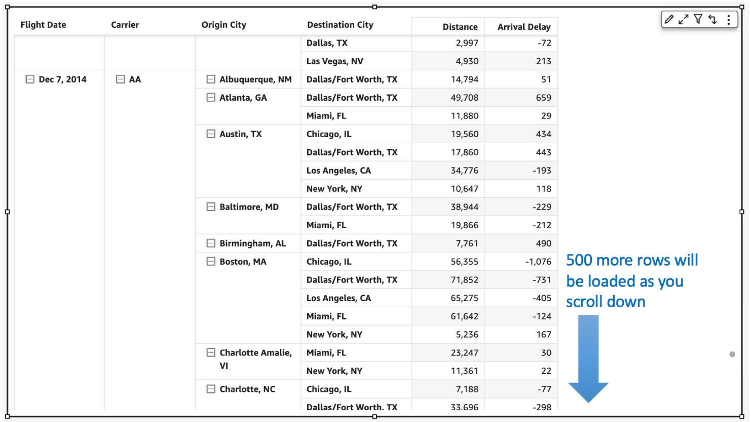
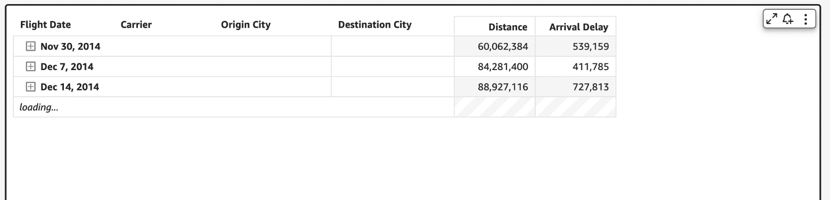
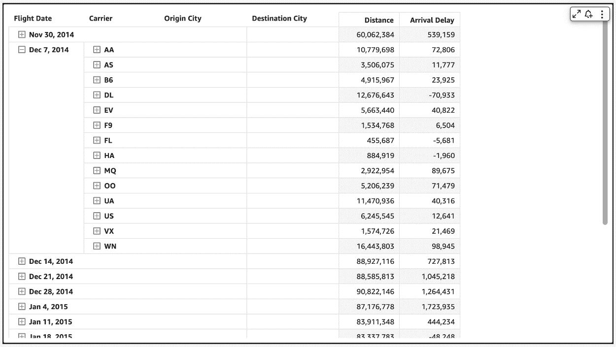


 Bhupinder Chadha is a senior product manager for Amazon QuickSight focused on visualization and front end experiences. He is passionate about BI, data visualization and low-code/no-code experiences. Prior to QuickSight he was the lead product manager for Inforiver, responsible for building a enterprise BI product from ground up. Bhupinder started his career in presales, followed by a small gig in consulting and then PM for xViz, an add on visualization product.
 Igal Mizrahi is a Senior Software Engineer for AWS QuickSight Charting team. He has been part of the team for the past 3 years, and previously worked on Amazon’s mobile shopping application for 4 years.
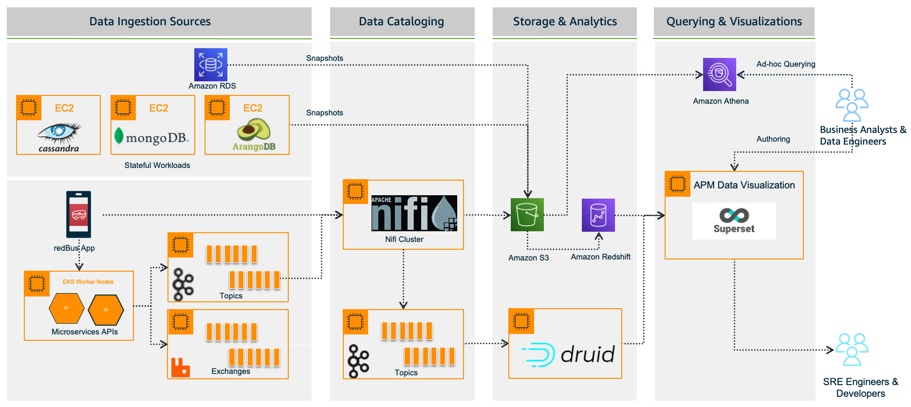
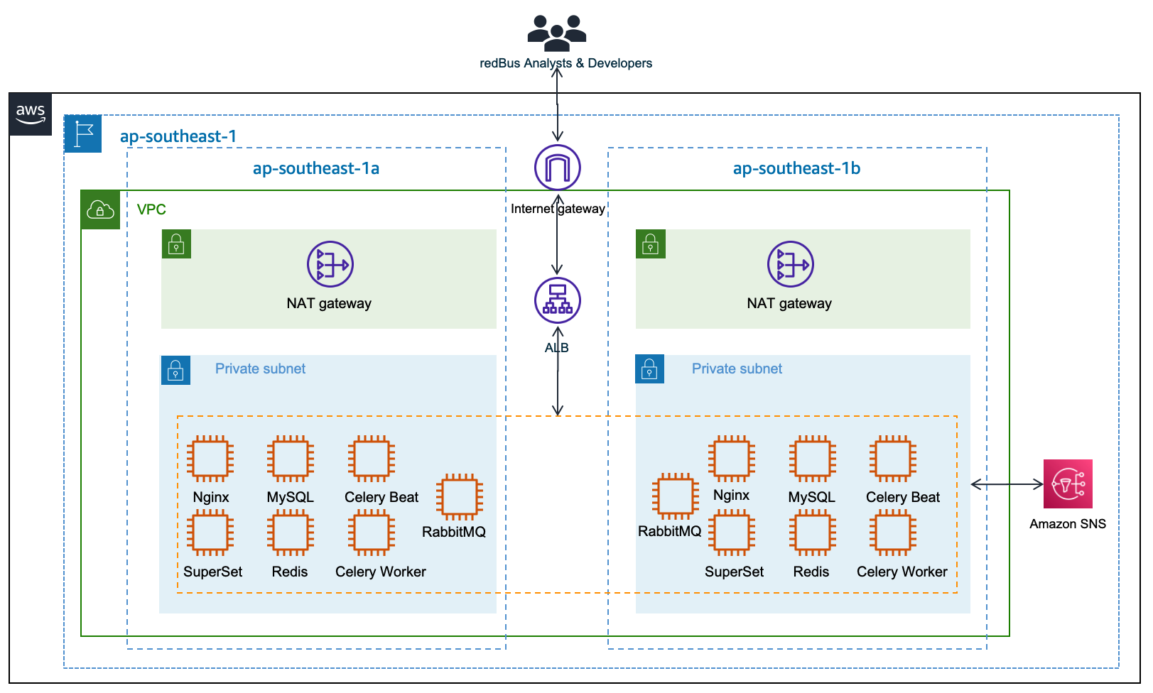
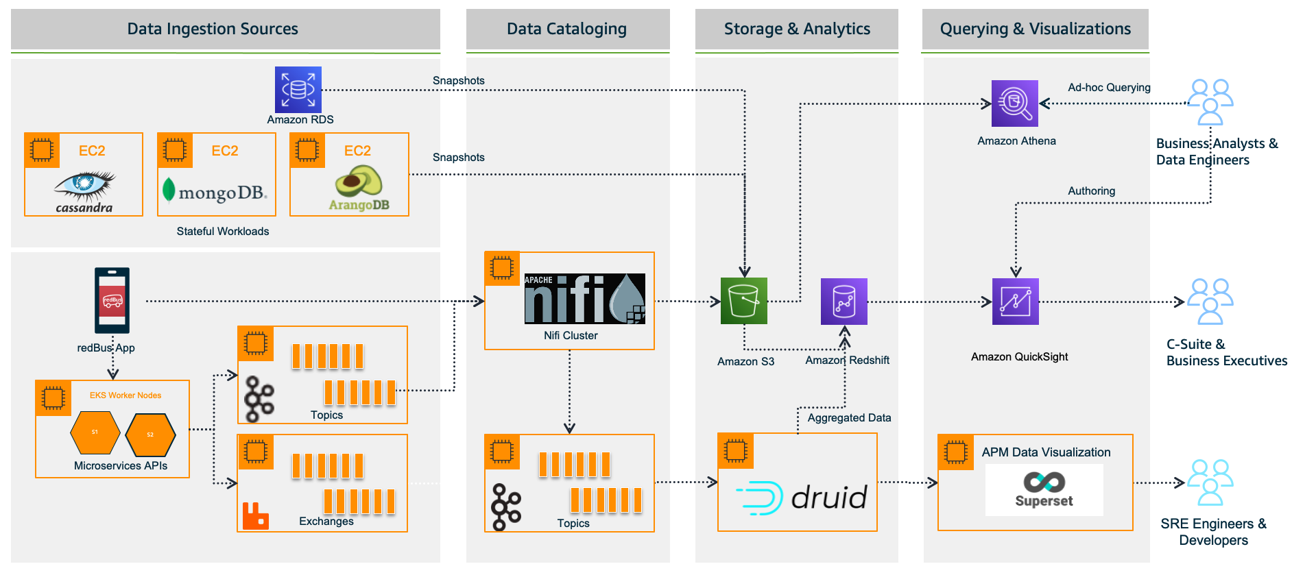
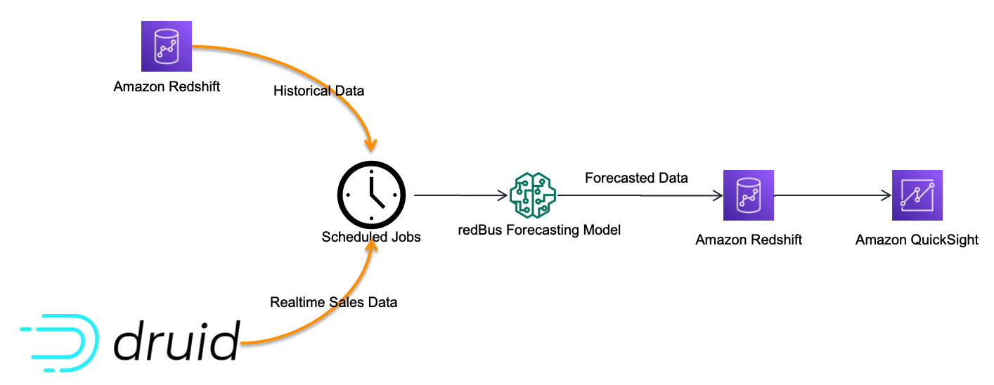
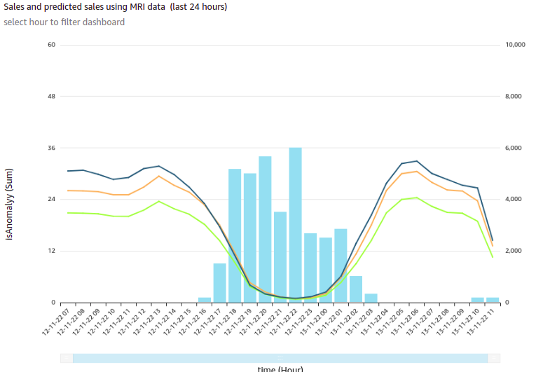


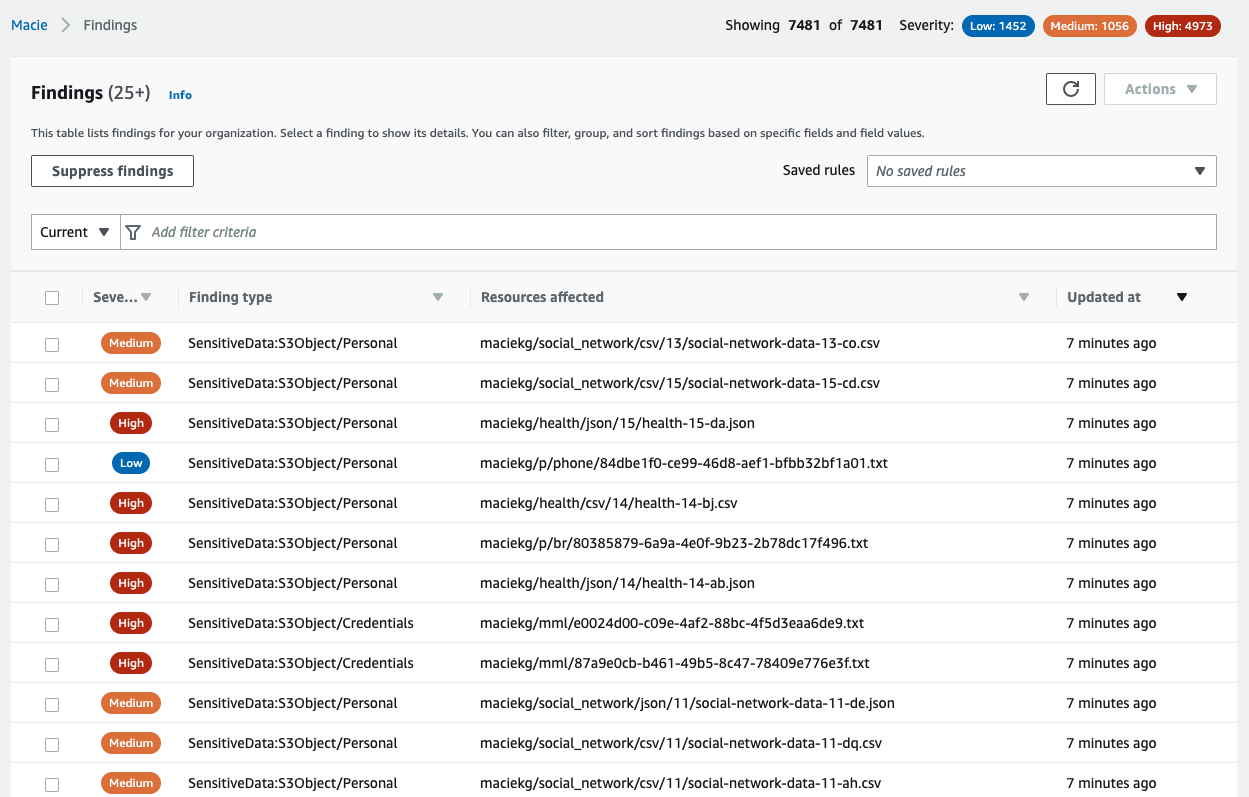
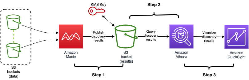
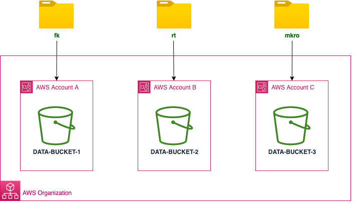


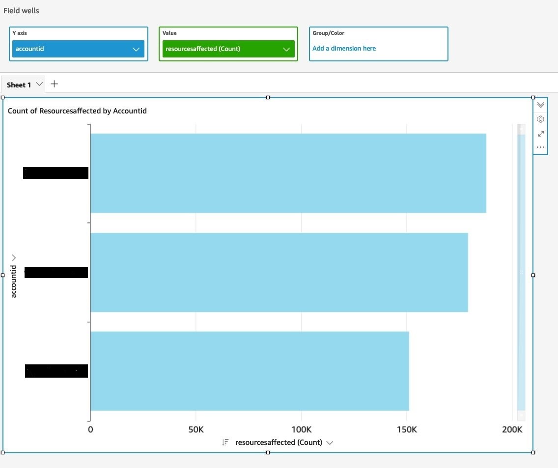
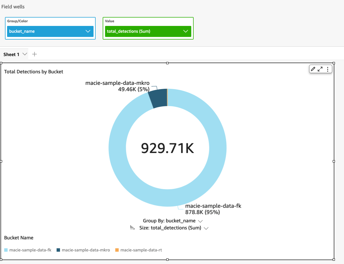
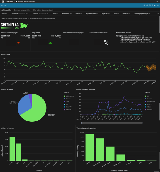
 Jeremy “Jez” Bristow is Head of Product at Green Flag. He has been working at Green Flag, part of Direct Line Group, for over 4 years and has been co-responsible for delivering the digital transformation programme within Green Flag. They have built a cloud-based ecosystem of micro-services supported by a data platform within AWS to enable the delivery of better customer outcomes to grow their business.
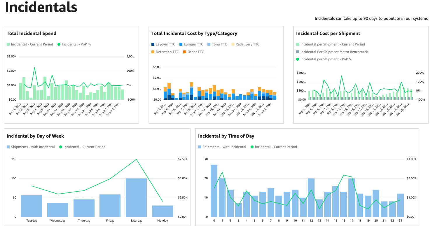
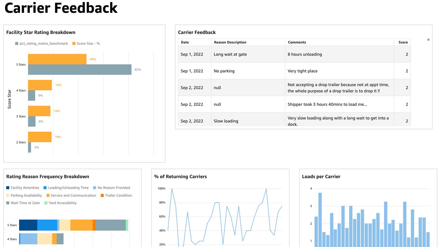
 Dorothy Li is Convoy’s CTO, overseeing Convoy’s Product and Engineering group and technology strategy, shaping and scaling the company’s innovation and industry-defining technology platforms. Prior to Convoy, Dorothy held leadership roles at Amazon, most recently as Vice President of BI and Analytics at AWS. During her more than 20 years at Amazon, Dorothy helped build out Amazon’s ecommerce platform and also led and collaborated on products that had visibly impacted customers around the world – from the initial launch of Amazon Prime, to Kindle, and at AWS where she focused on data analytics and BI. Dorothy received her Bachelor of Science at Brigham Young University and studies at Shanghai International Studies University.
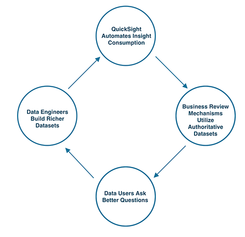
 Siamak Ziraknejad leads the technical product management team for Amazon Identity Services. His team formulates the technical product strategy and plans for account security (authentication and authorization across all surfaces, worldwide) and the consumer identity foundations for all Amazon programs and products (entitlement management, benefit sharing, and personalization).
 Abhinav Mehta is a Senior Product Manager (Technical) with the Amazon Identity Services team. He is focused on the product strategy and innovations for fast and secure authentication methods at Amazon.
 With more than 1.5 million unique users across 700 schools and core values that include connectivity, reliability, and innovation,
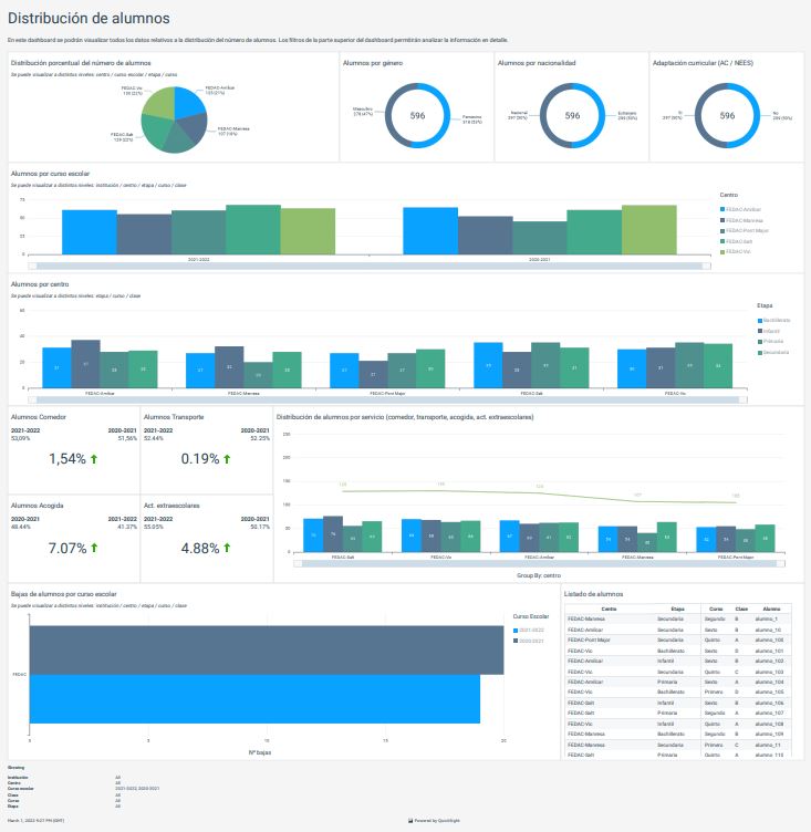
 Ignasi Nogués is the founder and the CTO of Clickedu. He is, by definition, a big entrepreneur and a dreamer. He drove the company since 2000 to success due to hard work. He always wants to take the next step.
 Georgina Valls is the Marketing Manager of Clickedu. She is a hardworker, dedicated to letting others know about Clickedu and its capabilities. As the daughter of teachers, she is very passionate about creating a brighter future in education.
 David Adamson is the head of WWSO Insights. He is leading the team on the journey to a data driven organization that delivers insightful, actionable data products to WWSO and shared in partnership with the broader AWS organization. In his spare time, he likes to travel across the world and can be found in his back garden, weather permitting exploring and photography the night sky.
 Yash Agrawal is an Analytics Lead at Amazon Web Services. Yash’s role is to define the analytics roadmap, develop standardized global dashboards & deliver insightful analytics solutions for stakeholders across AWS.
 Addis Crooks-Jones is a Sr. Manager of Business Intelligence Engineering at Amazon Web Services Finance, Analytics and Science Team (FAST). She is responsible for partnering with business leaders in the World Wide Specialist Organization to build a culture of data to support strategic initiatives. The technology solutions developed are used globally to drive decision making across AWS. When not thinking about new plans involving data, she like to be on adventures big and small involving food, art and all the fun people in her life.
 Graham Gilvar is an Analytics Lead at Amazon Web Services. He builds and maintains centralized QuickSight dashboards, which enable stakeholders across all WWSO services to interlock and make data driven decisions. In his free time, he enjoys walking his dog, golfing, bowling, and playing hockey.
 Shilpa Koogegowda is the Sales Ops Analyst at Amazon Web Services and has been part of the WWSO Insights team for the last two years. Her role involves building standardized metrics, dashboards and data products to provide data and insights to the customers.
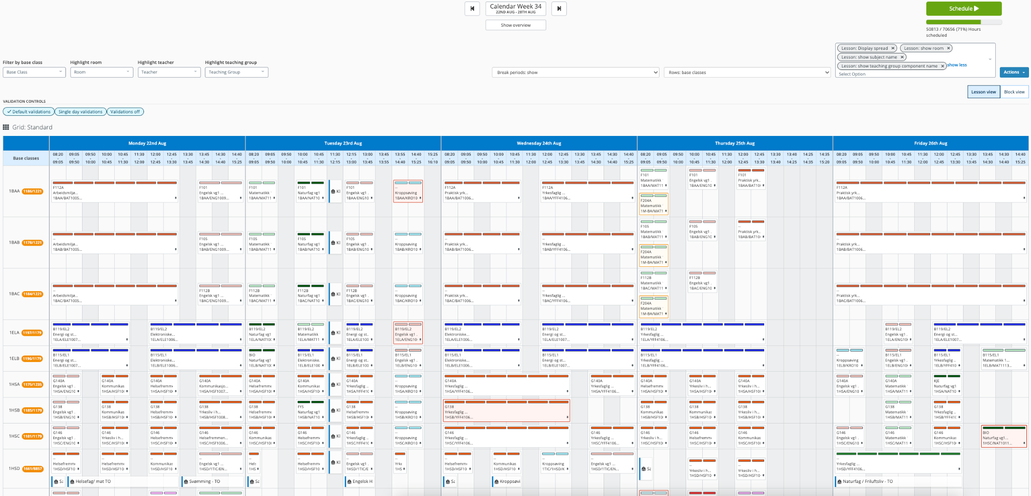
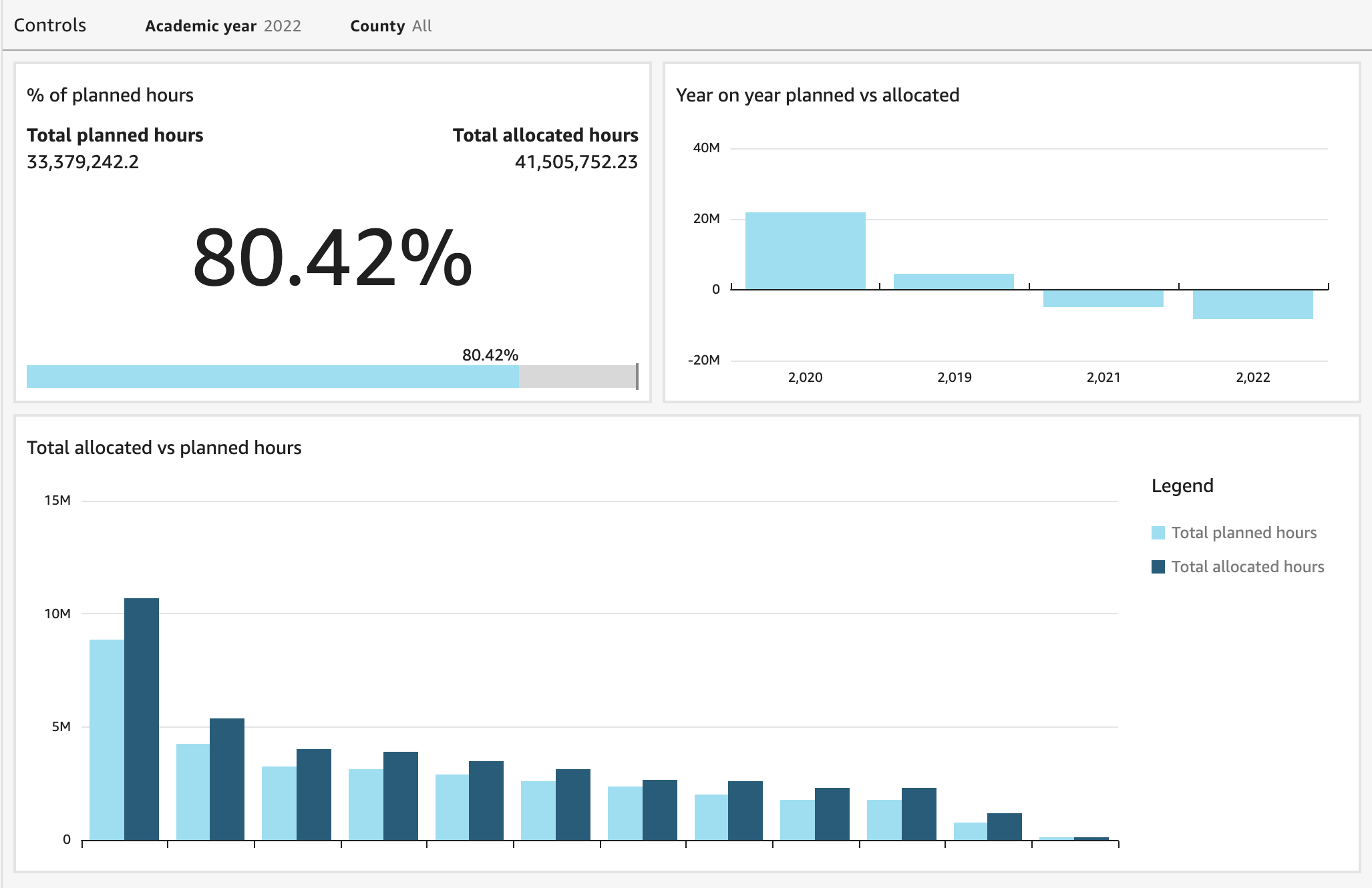
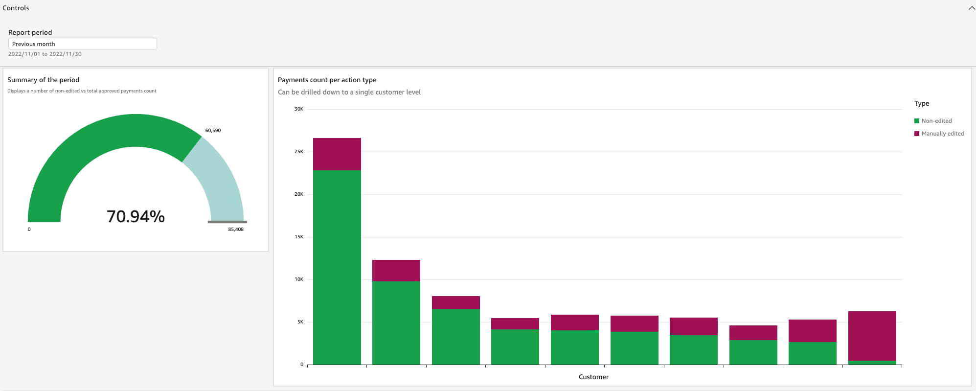


 Vasily Ulianko is a Director of Engineering in Visma InSchool, leading the development and operations, focusing on building strong engineering culture and solid system design.
 Per Brandser is a Product Strategy Manager in Visma InSchool. Mainly focusing on coaching our Product Managers on vision, product strategy and product discovery methodology, Per is a promoter of data driven product management.
 Tomotaka Inoue is a data analyst at Leverages. Tomotaka analyzes Levtech’s data and suggests about the strategy and marketing.
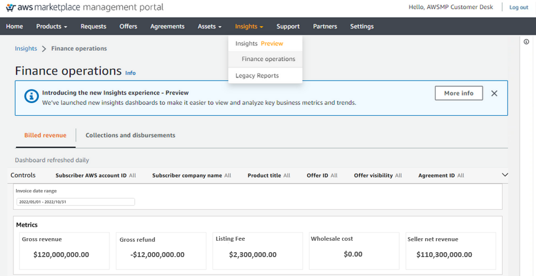
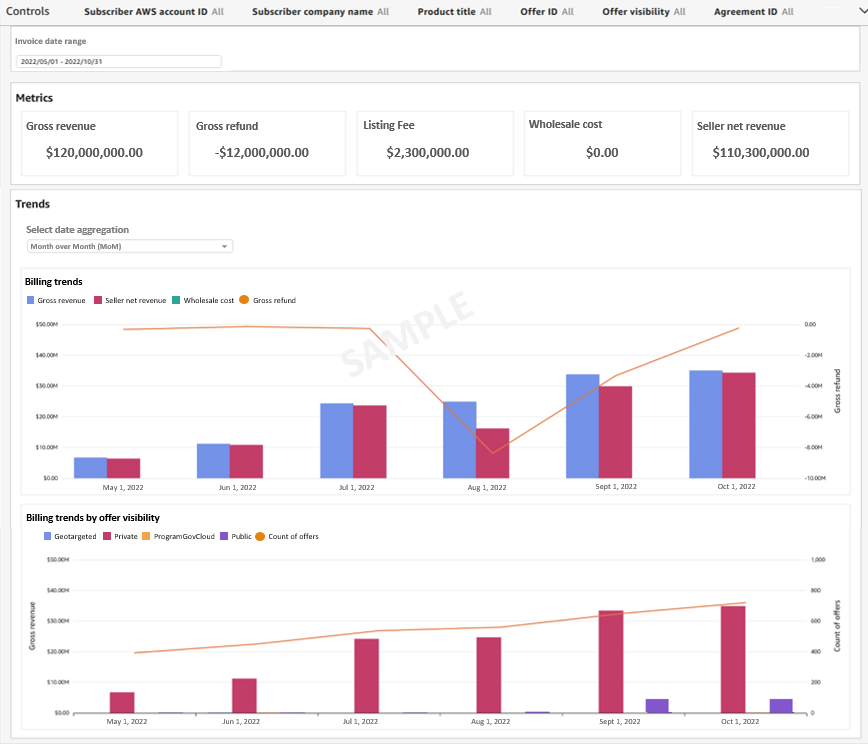
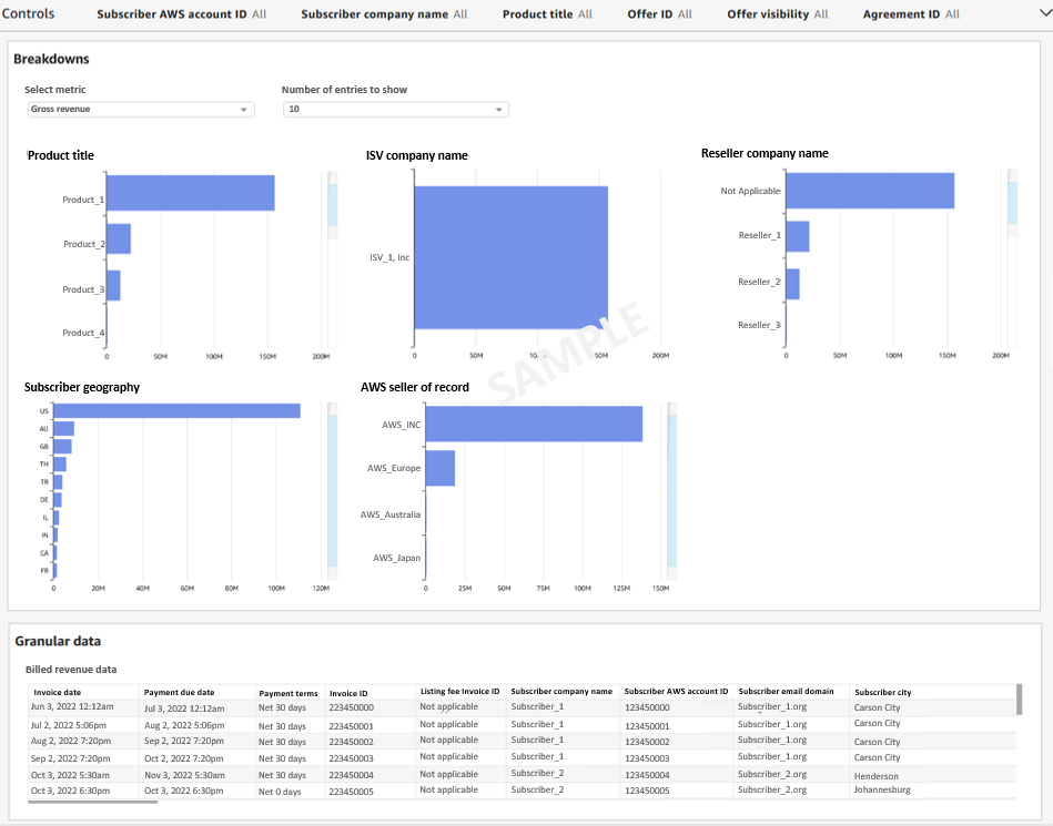
 Snigdha Sahi is a Senior Product Manager (Technical) with Amazon Web Services (AWS) Marketplace. She has diverse work experience across product management, product development and management consulting. A technology enthusiast, she loves brainstorming and building products that are intuitive and easy to use. In her spare time, she enjoys hiking, solving Sudoku and listening to music.
 Vincent Larchet is a Principal Software Development Engineer on the AWS Marketplace team based in Vancouver, BC. Outside of work, he is a passionate wood worker and DIYer.


 Srikanth Baheti is a Specialized World Wide Sr. Solution Architect for Amazon QuickSight. He started his career as a consultant and worked for multiple private and government organizations. Later he worked for PerkinElmer Health and Sciences & eResearch Technology Inc, where he was responsible for designing and developing high traffic web applications, highly scalable and maintainable data pipelines for reporting platforms using AWS services and Serverless computing.
 Raji Sivasubramaniam is a Sr. Solutions Architect at AWS, focusing on Analytics. Raji is specialized in architecting end-to-end Enterprise Data Management, Business Intelligence and Analytics solutions for Fortune 500 and Fortune 100 companies across the globe. She has in-depth experience in integrated healthcare data and analytics with wide variety of healthcare datasets including managed market, physician targeting and patient analytics.

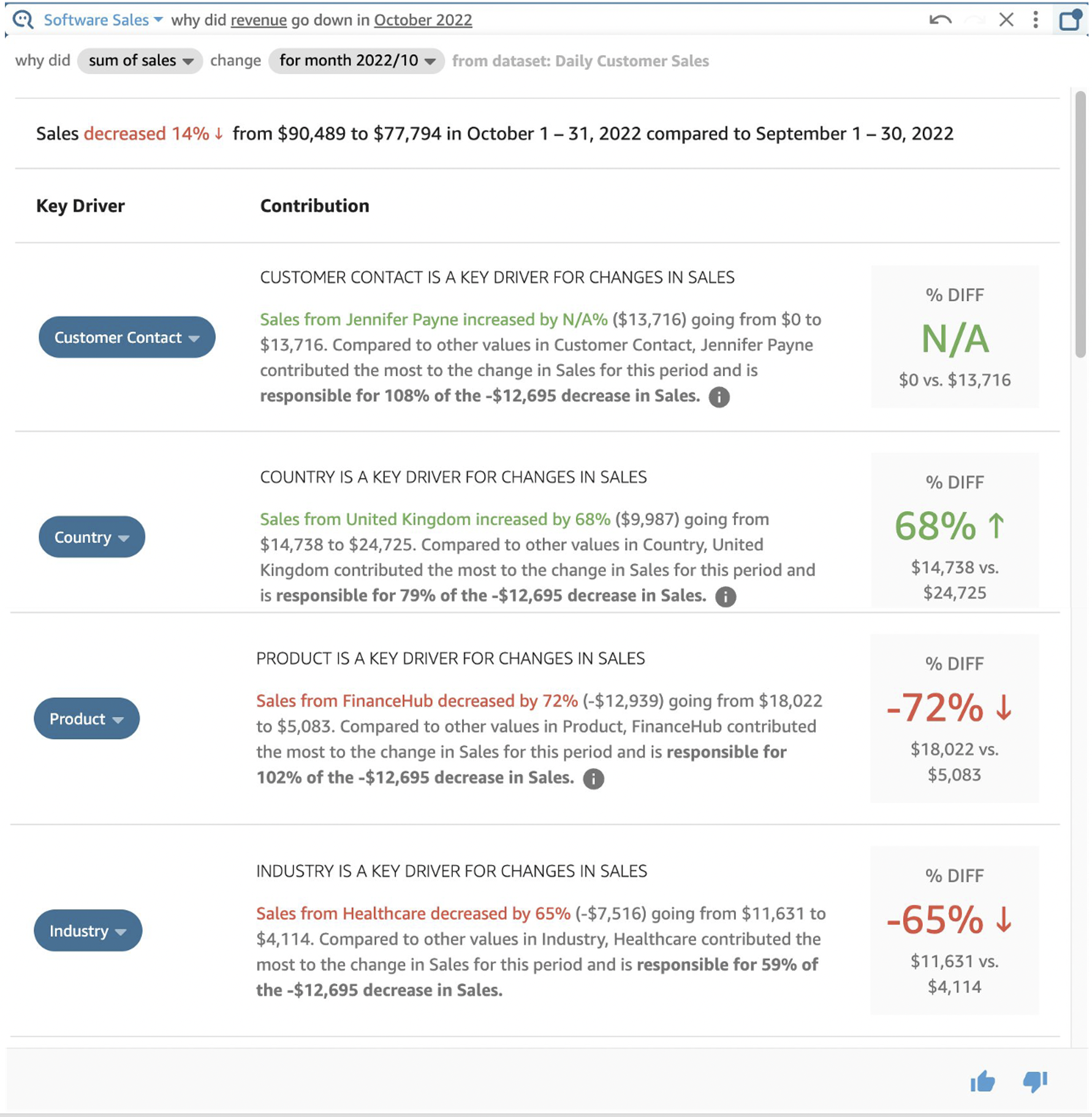
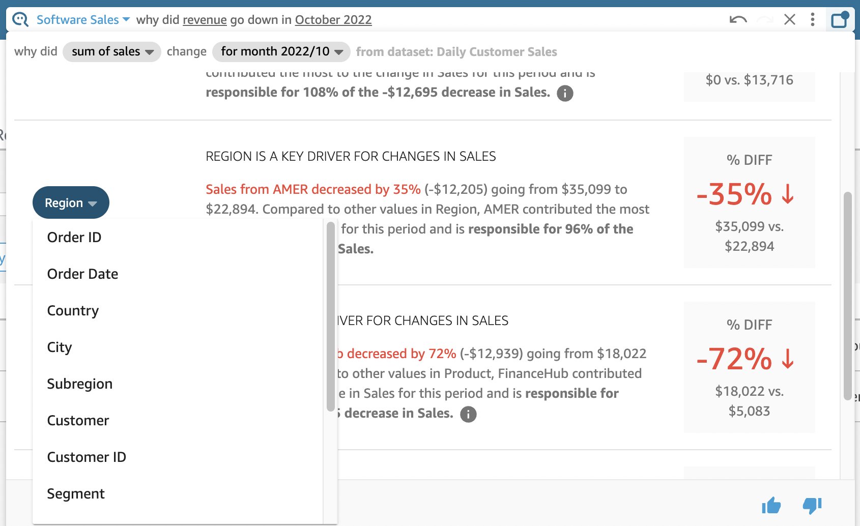


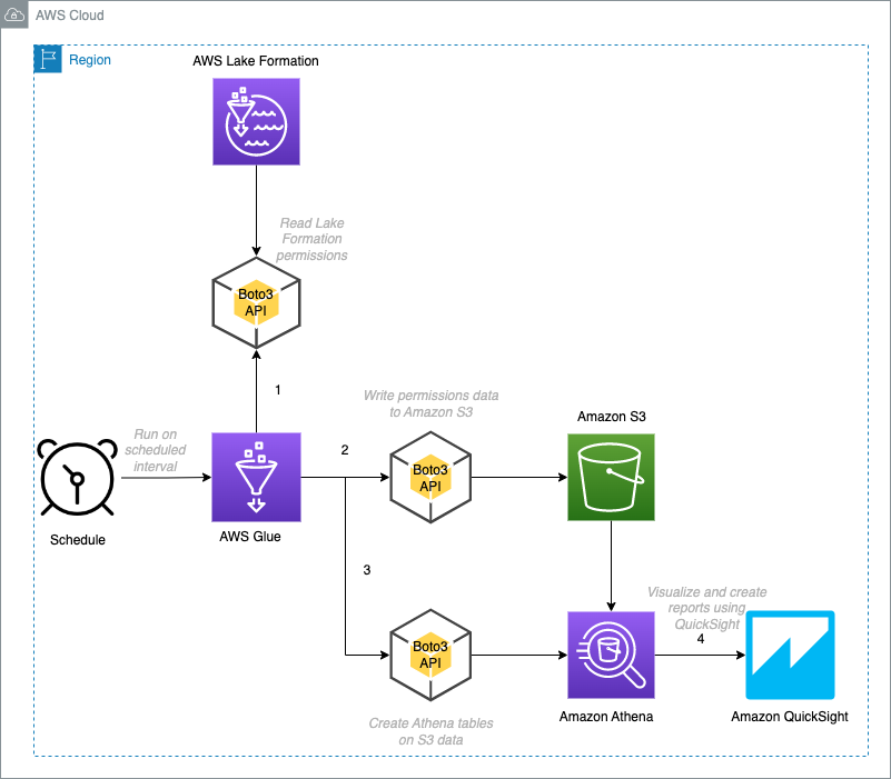


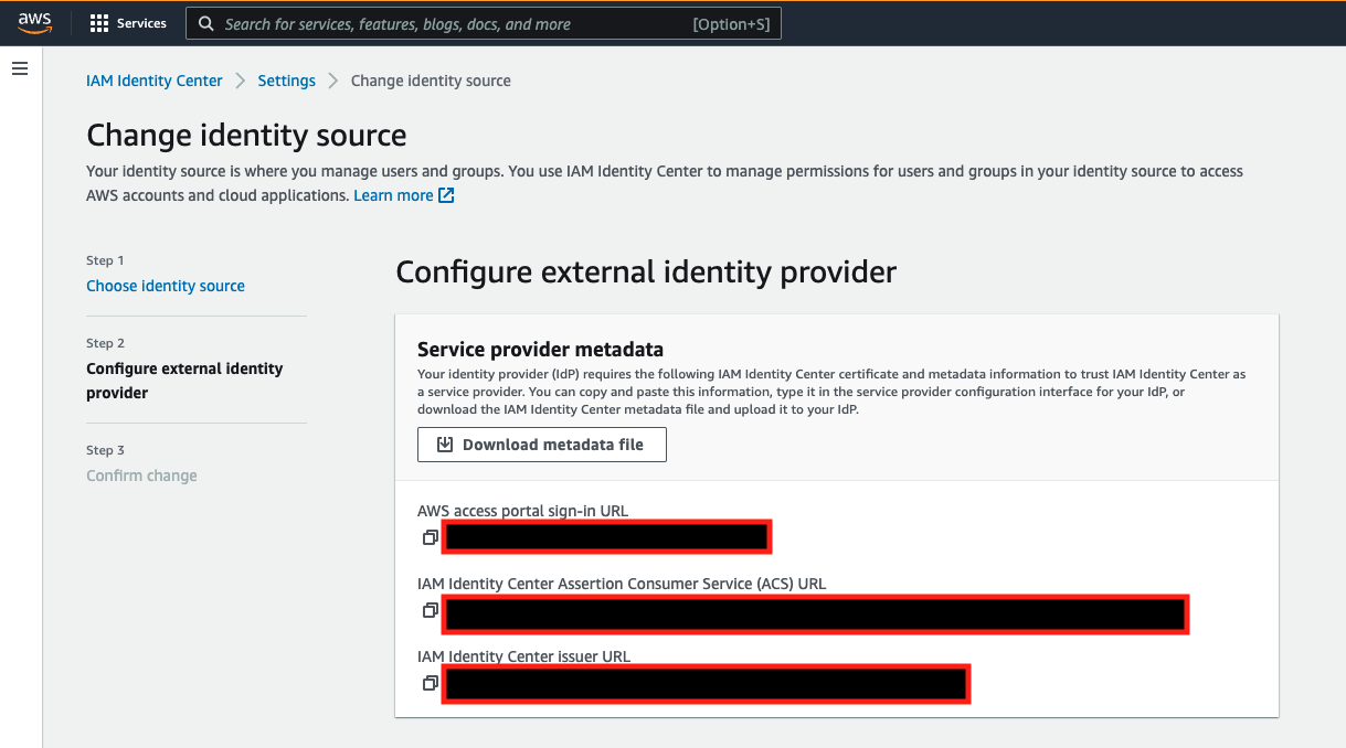


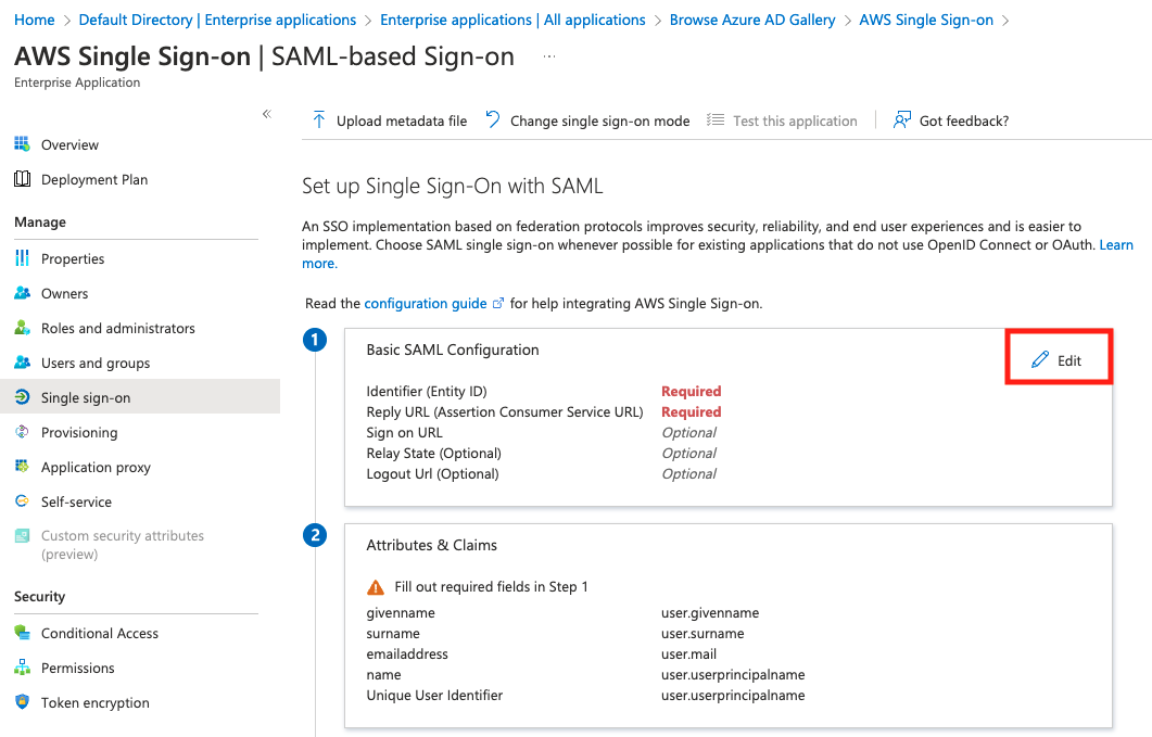


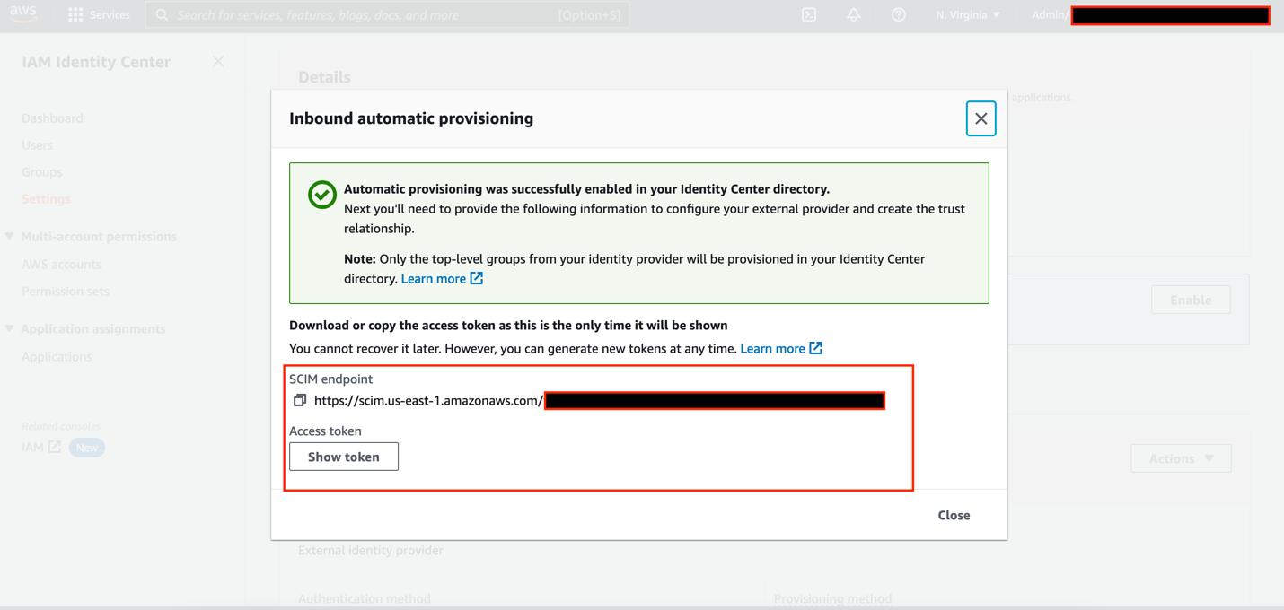

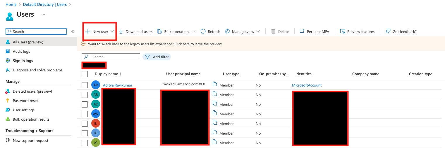
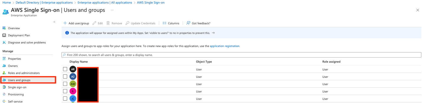
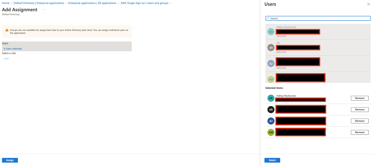
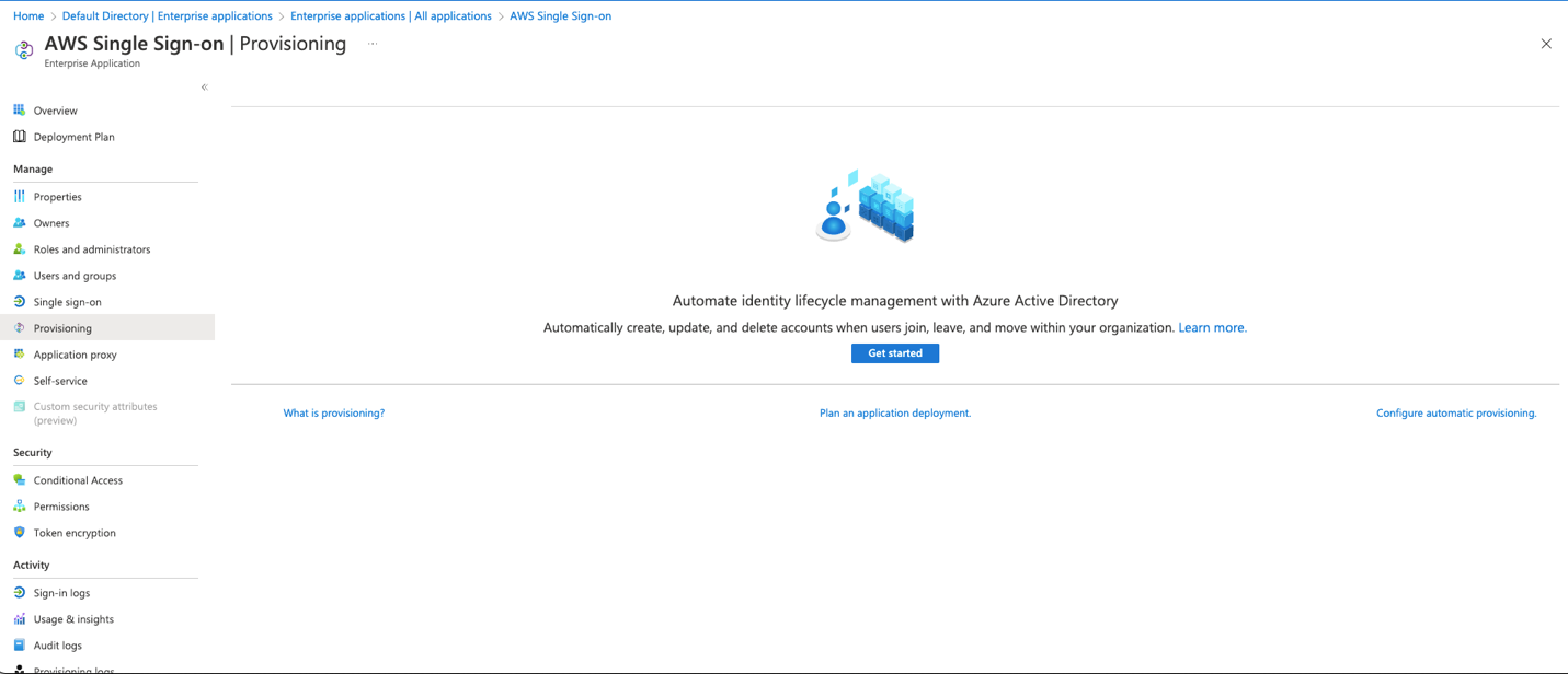


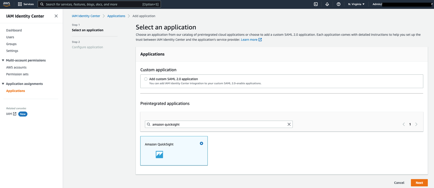


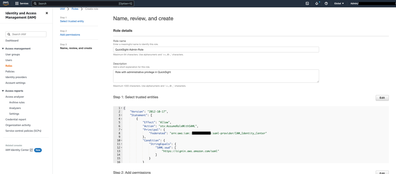


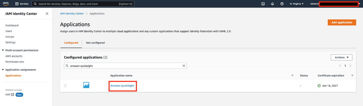
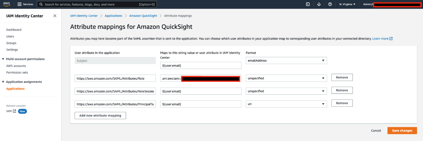


 Aditya Ravikumar is a Solutions Architect at Amazon Web Services. He is based in Seattle, USA. Aditya’s core interests include software development, databases, data analytics and machine learning. He works with AWS customers/partners to provide guidance and technical assistance to transform their business through innovative use of cloud technologies.
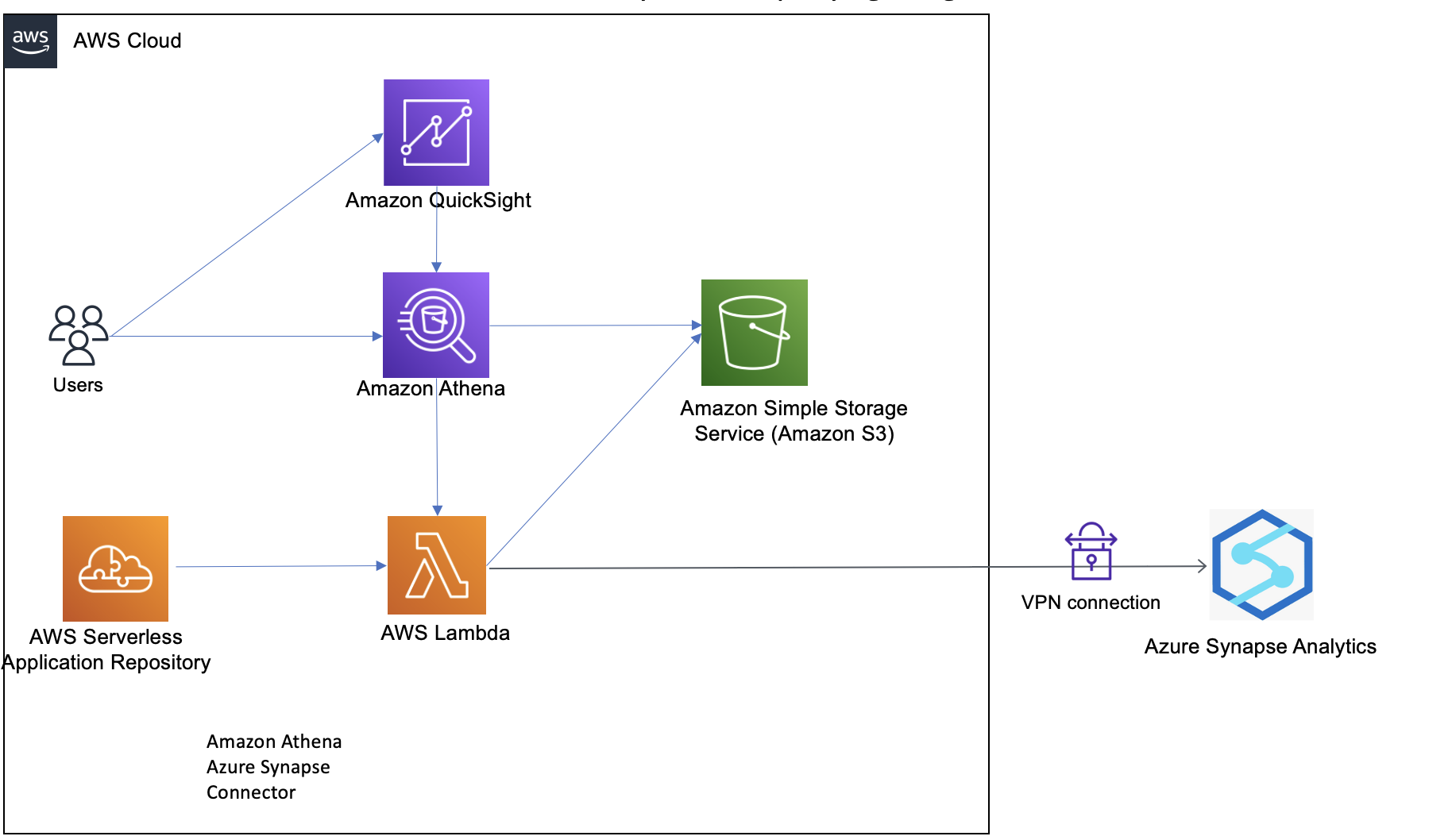
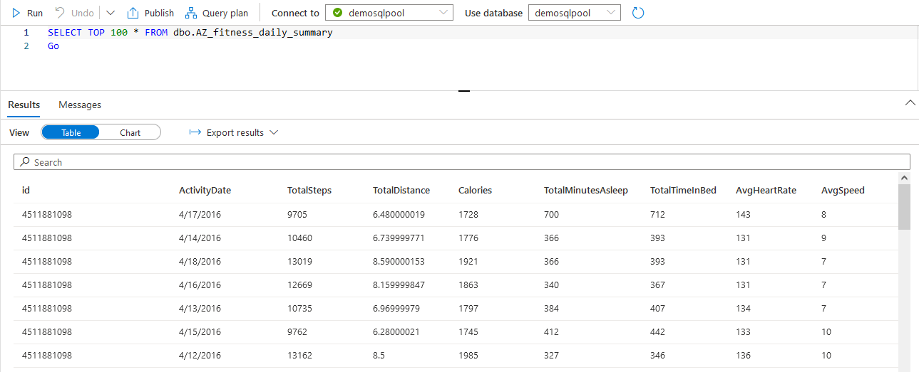

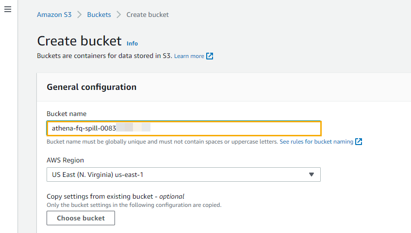
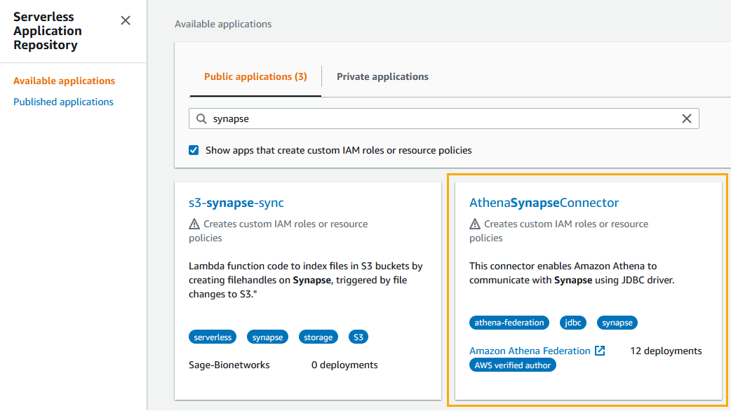
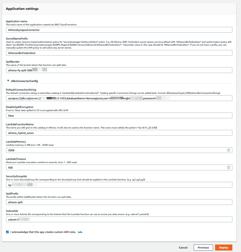
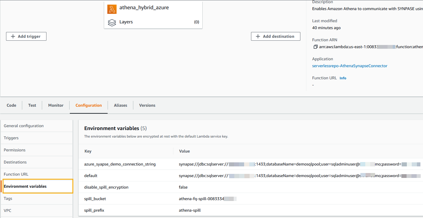
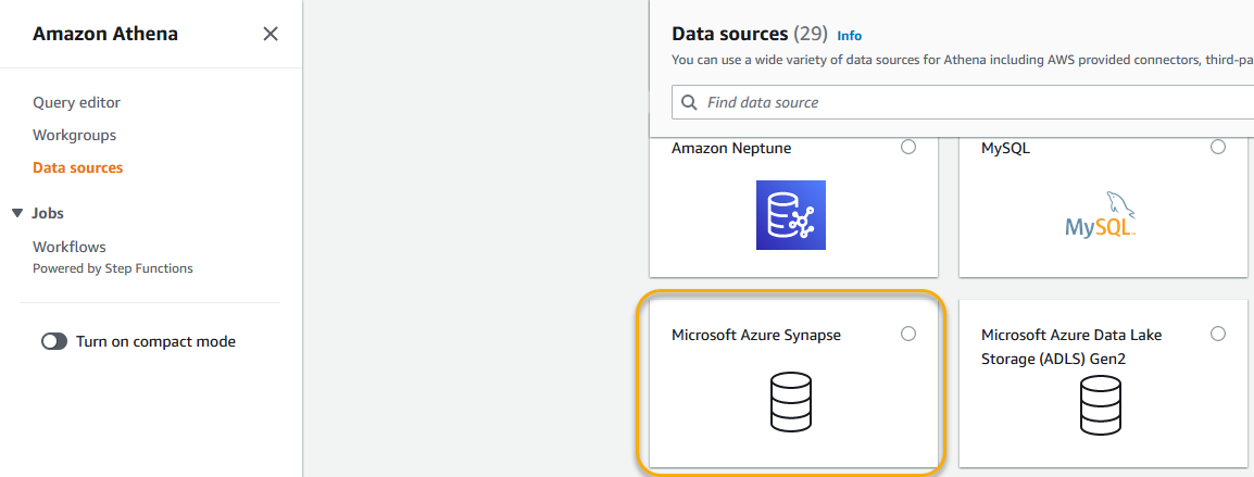


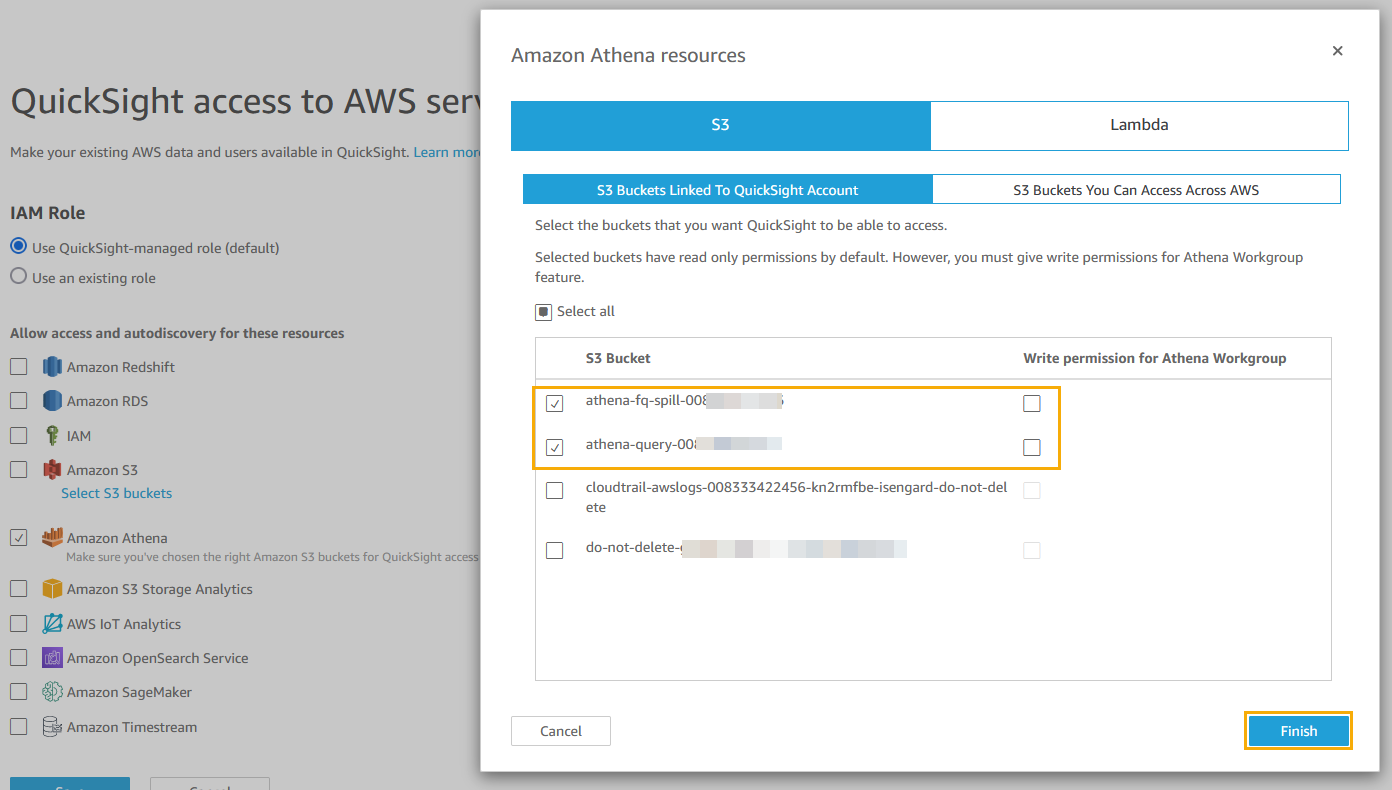


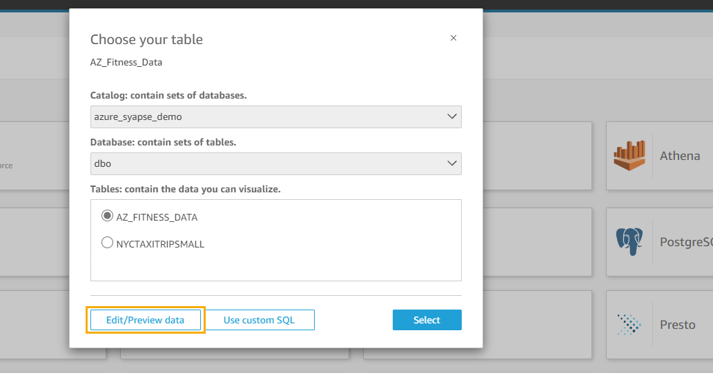


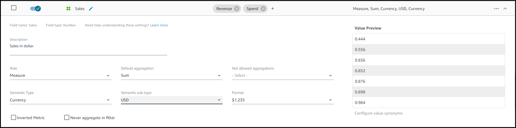


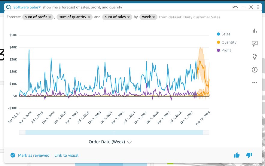
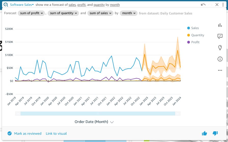
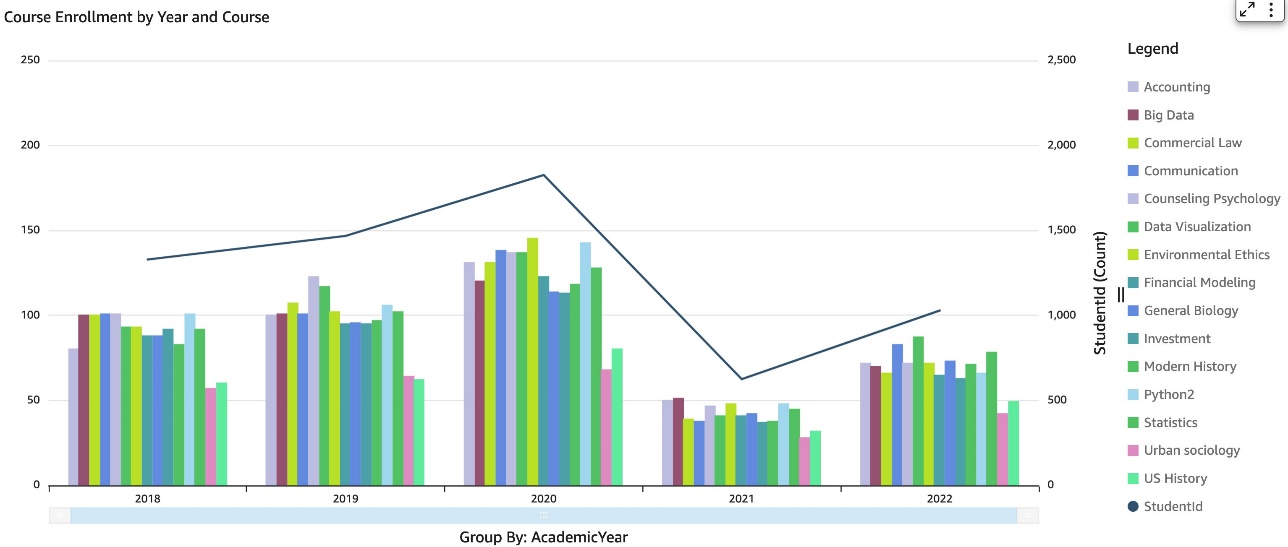
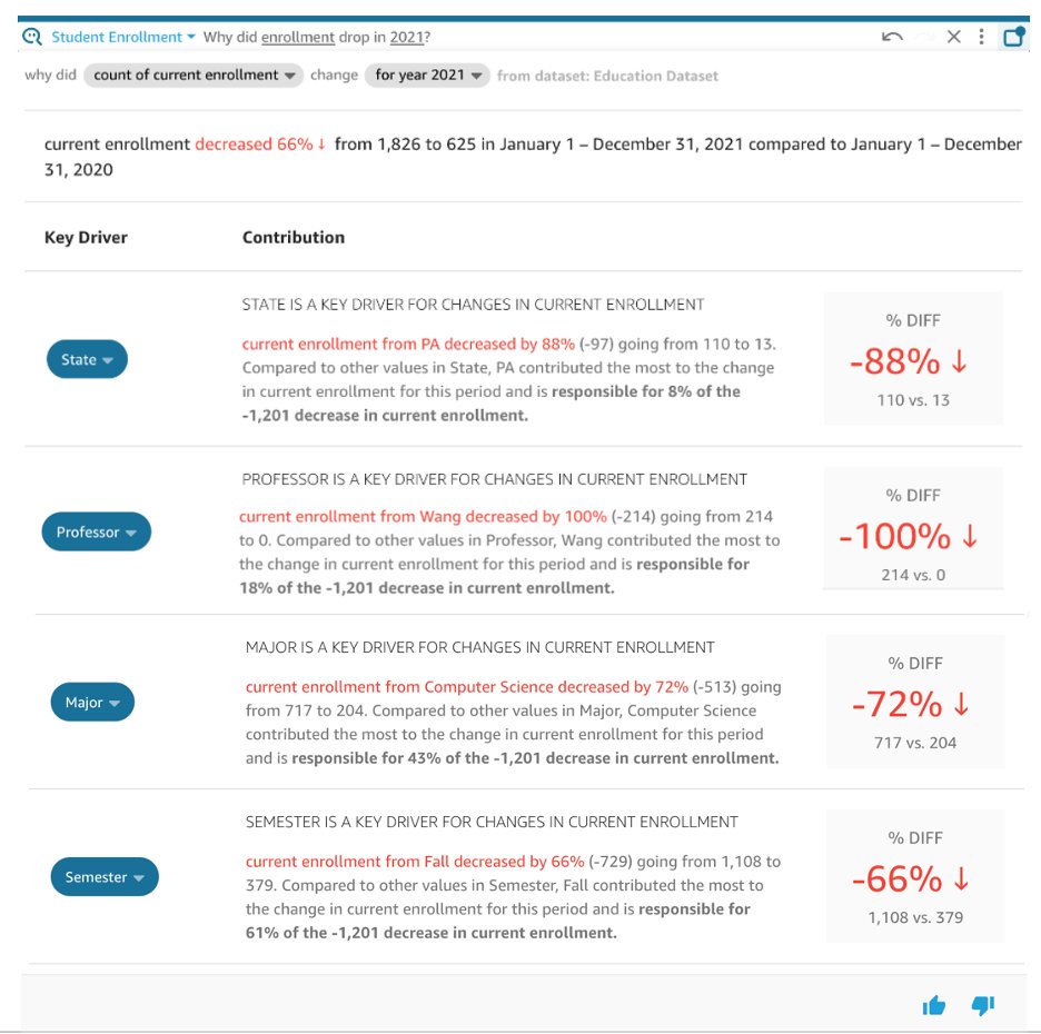
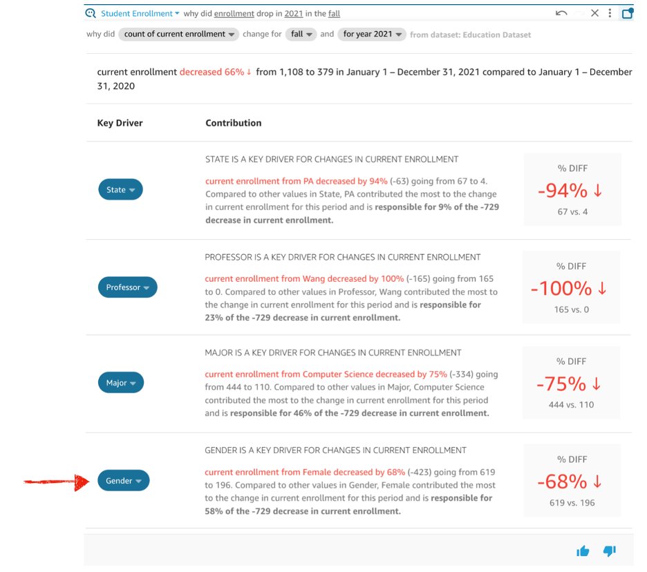
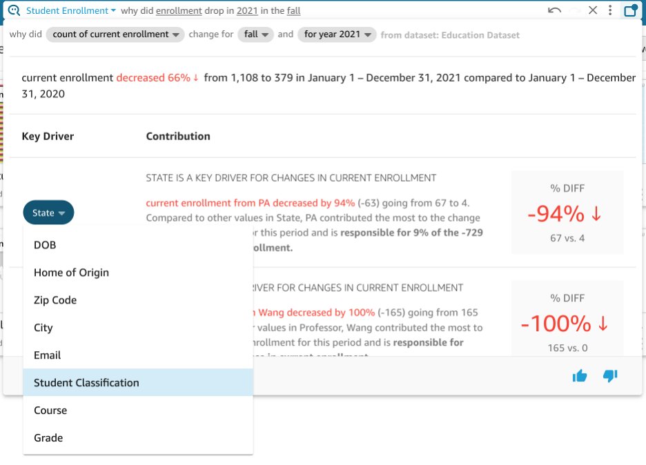
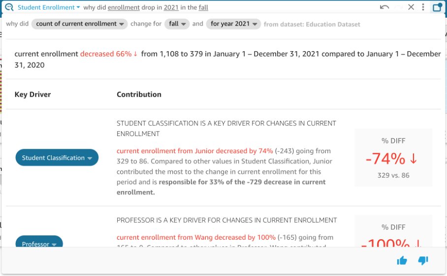
 Shannon Kalisky is a Senior Product Manager – Technical that covers natural language question patterns and model robustness for Amazon QuickSight Q.