Tag Archives: Analytics

Get started with Amazon Redshift cross-database queries (preview)

Post Syndicated from Neeraja Rentachintala original https://aws.amazon.com/blogs/big-data/get-started-with-amazon-redshift-cross-database-queries-preview/

Amazon Redshift is a fast, scalable, secure, and fully managed cloud data warehouse that makes it simple and cost-effective to analyze all your data using standard SQL and your existing ETL, business intelligence (BI), and reporting tools. Tens of thousands of customers use Amazon Redshift to process exabytes of data per day and power analytics workloads such as BI, predictive analytics, and real-time streaming analytics.

We’re excited to announce the public preview of the new cross-database queries capability to query across databases in an Amazon Redshift cluster. In this post, we provide an overview of the cross-database queries and a walkthrough of the key functionality that allows you to manage data and analytics at scale in your organization.

What are cross-database queries?

With cross-database queries, you can seamlessly query data from any database in your Amazon Redshift cluster, regardless of which database you’re connected to. Cross-database queries eliminate data copies and simplify your data organization to support multiple business groups on the same cluster. Support for cross-database queries is available on Amazon Redshift RA3 node types.

Data is organized across multiple databases in Amazon Redshift clusters to support multi-tenant configurations. However, you often need to query and join across these datasets by allowing read access. For example, different business groups and teams that own and manage their datasets in a specific database in the data warehouse need to collaborate with other groups. You might want to perform common ETL staging and processing while your raw data is spread across multiple databases. Organizing data in multiple Amazon Redshift databases is also a common scenario when migrating from traditional data warehouse systems.

With cross-database queries, you can now access data from any database on the Amazon Redshift cluster without having to connect to that specific database. You can also join datasets from multiple databases in a single query. You can access database objects such as tables, views with a simple three-part notation of <database>.<schema>.<object>, and analyze the objects using business intelligence (BI) or analytics tools. You can continue to set up granular access controls for users with standard Amazon Redshift SQL commands and ensure that users can only see the relevant subsets of the data they have permissions for.

Walkthrough overview

In this post, we walk through an end-to-end use case to illustrate cross-database queries, comprising the following steps:

  1. Set up permissions on the data.
  2. Access data and perform several cross-database queries.
  3. Connect from tools.

For this walkthrough, we use SQL Workbench, a SQL query tool, to perform queries on Amazon Redshift. For more information about connecting SQL Workbench to an Amazon Redshift cluster, see Connect to your cluster by using SQL Workbench/J .

Setting up permissions for cross-database queries

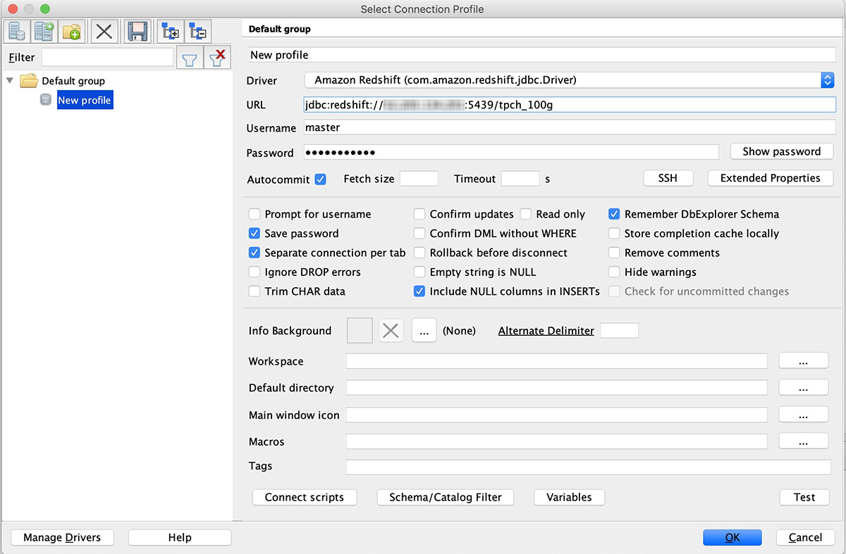
You can use standard Redshift SQL GRANT and REVOKE commands to configure appropriate permissions for users and groups. To configure permissions, we connect as an administrator to a database named TPCH_100G on an Amazon Redshift cluster that we set up with an industry standard dataset, TPC-H. You can set up this dataset in your environment using the code and scripts for this dataset on GitHub and the accompanying dataset hosted in a public Amazon Simple Storage Service (Amazon S3) bucket.

The following screenshot shows the configuration for your connection profile.

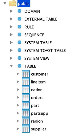
The TPCH_100G database consists of eight tables loaded in the schema PUBLIC, as shown in the following screenshot.

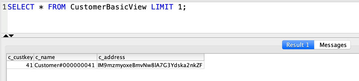
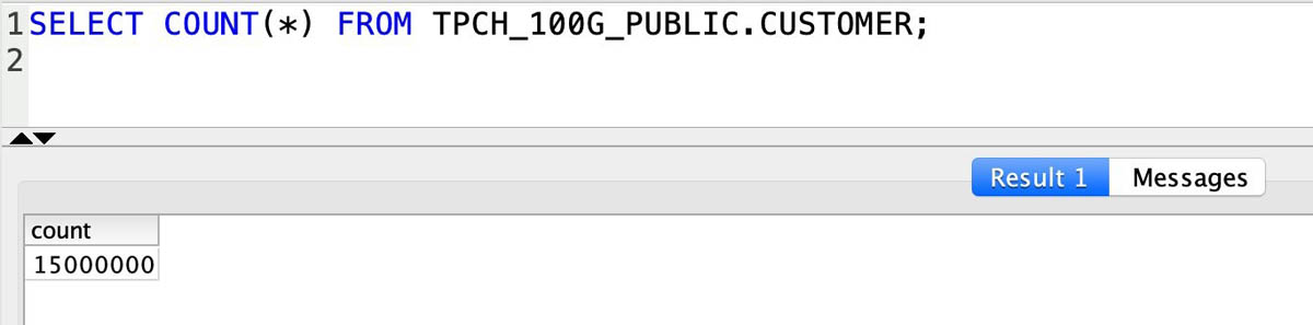
The following screenshot shows a test query on one of the TPC-H tables, customer.

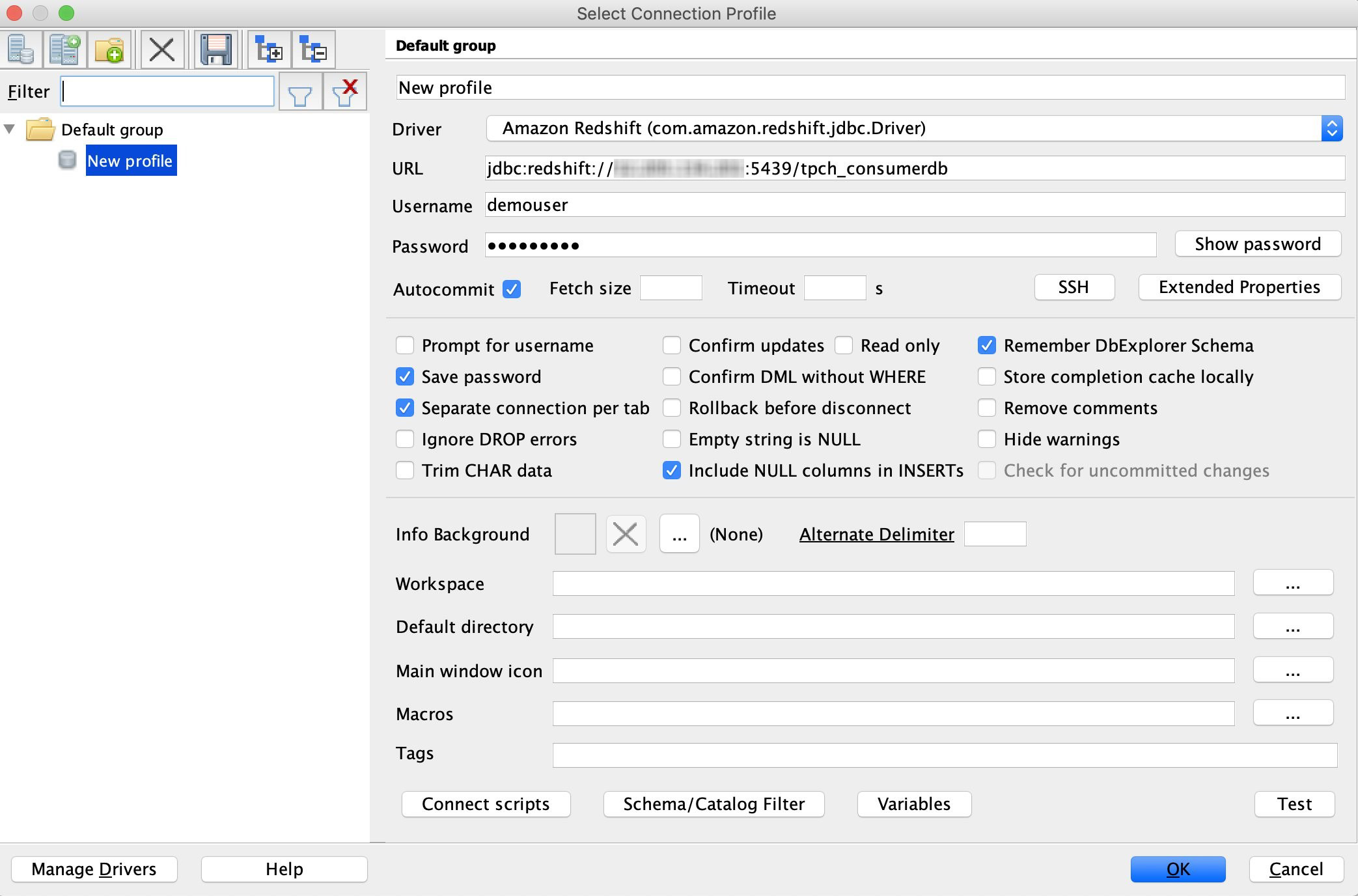
The database administrator provides read permissions on the three of the tables, customer, orders, and lineitem, to an Amazon Redshift user called demouser. The user typically connects to and operates in their own team’s database TPCH_CONSUMERDB on the same Amazon Redshift cluster.

Performing cross-database queries using three-part notation

In this section, we see how cross-database queries work in action. With cross-database queries, you can connect to any database and query from all the other databases in the cluster without having to reconnect. In this use case, the user demouser connects to their database TPCH_CONSUMERDB (see the following screenshot).

While connected to TPCH_CONSUMERDB, demouser can also perform queries on the data in TPCH_100gG database objects that they have permissions to, referring to them using the simple and intuitive three-part notation TPCH_100G.PUBLIC.CUSTOMER (see the following screenshot).

You can refer to and query objects in any other database in the cluster using this <database>.<schema>.<object> notation as long as you have permissions to do so. The objects can be tables or views (including regular, late binding and materialized views).

In addition to performing queries on objects, you can create views on top of objects in other databases and apply granular access controls as relevant.

Joining data across databases

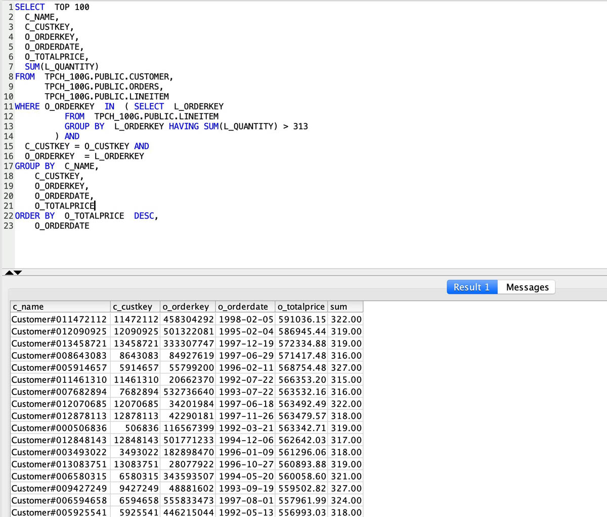
With cross-database queries, you can join datasets across databases. In the following screenshot, demouser queries and performs joins across the customer, lineitem, and orders tables in the TPCH_100G database.

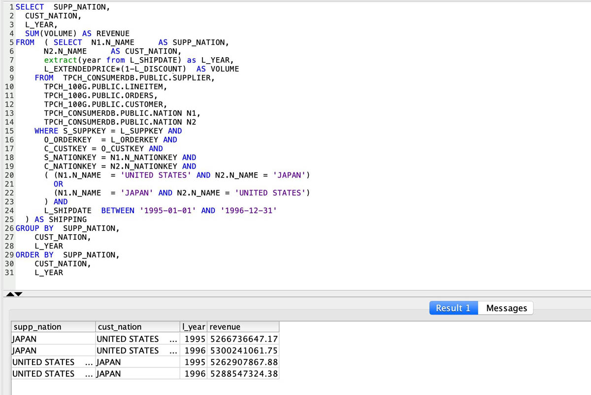
You can also span joins on objects across databases. In the following query, demouser seamlessly joins the datasets from TPCH_100G (customer, lineitem, and orders tables) with the datasets in TPCH_CONSUMERDB (nation and supplier tables).

With cross-database queries, you get a consistent view of the data irrespective of the database you’re connected to.

Securely accessing relevant datasets by connecting from tools

To support the database hierarchy navigation and exploration introduced with cross-database queries, Amazon Redshift is introducing a new set of metadata views and modified versions of JDBC and ODBC drivers.

In addition, you can create aliases from one database to schemas in any other databases on the Amazon Redshift cluster. You create the aliases using the CREATE EXTERNAL SCHEMA command, which allows you to refer to the objects in cross-database queries with the two-part notation <external schema name>.<object>. For example, in the following screenshot, the database administrator connects to TPCH_CONSUMERDB and creates an external schema alias for the PUBLIC schema in TPC_100G database called TPC_100G_PUBLIC and grants the usage access on the schema to demouser.

Now, when demouser connects to TPCH_CONSUMERDB, they see the external schema in the object hierarchy (as in the following screenshot) with only the relevant objects that they have permissions to: CUSTOMER, LINEITEM, and ORDERS.

Now they can perform queries using the schema alias as if the data is local rather than using a three-part notation.

Summary and next steps

We provided you a glimpse into what you can accomplish with cross-database queries in Amazon Redshift. Cross-database queries allow you to organize and manage data across databases to effectively support multi-tenant data warehouse deployments for a wide variety of use cases. You can get started with your use case leveraging cross-database queries capability by trying out the preview. For more information, refer to the documentation cross-database queries.


About the Authors

Neeraja Rentachintala is a Principal Product Manager with Amazon Redshift. Neeraja is a seasoned Product Management and GTM leader, bringing over 20 years of experience in product vision, strategy and leadership roles in data products and platforms. Neeraja delivered products in analytics, databases, data Integration, application integration, AI/Machine Learning, large scale distributed systems across On-Premise and Cloud, serving Fortune 500 companies as part of ventures including MapR (acquired by HPE), Microsoft SQL Server, Oracle, Informatica and Expedia.com.


Jenny Chen is a senior database engineer at Amazon Redshift focusing on all aspects of Redshift performance, like Query Processing, Concurrency, Distributed system, Storage, OS and many more. She works together with development team to ensure of delivering highest performance, scalable and easy-of-use database for customer. Prior to her career in cloud data warehouse, she has 10-year of experience in enterprise database DB2 for z/OS in IBM with focus on query optimization, query performance and system performance.


Sushim Mitra is a software development engineer on the Amazon Redshift query processing team. His interest areas are Query Optimization problems, SQL Language features and Database security. When not at work, he enjoys reading fiction from all over the world.


Suzhen Lin is a senior software development engineer on the Amazon Redshift transaction processing and storage team. Suzhen Lin has over 15 years of experiences in industry leading analytical database products including AWS Redshift, Gauss MPPDB, Azure SQL Data Warehouse and Teradata as senior architect and developer. Her experiences cover storage, transaction processing, query processing, memory/disk caching and etc in on-premise/cloud database management systems.


Analyzing healthcare FHIR data with Amazon Redshift PartiQL

Post Syndicated from Amir Bar Or original https://aws.amazon.com/blogs/big-data/analyzing-healthcare-fhir-data-with-amazon-redshift-partiql/

Healthcare organizations across the globe strive to provide the best possible patient care at the lowest cost. In a patient’s care journey, multiple organizations are often involved, including the healthcare provider, diagnostic labs, pharmacies, and health insurance payors. Each of these organizations needs to exchange health data efficiently with the others to ensure care continuity and reimbursement.

The healthcare industry has adopted data exchange standards, many of which are defined by Health Level Seven International (HL7), for several decades. HL7v2, a pipe-delimited data format developed three decades ago, is still in use today despite not conforming to modern best practices for communicating between systems, such as with RESTful APIs. Naturally, these shortcomings can complicate interoperability. More recently, HL7 introduced FHIR (Fast Healthcare Interoperability Resources) to help solve some of the complexity and pave the way for healthcare organizations to modernize how they exchange information. FHIR is built around resources that logically organize healthcare information in a structured but fully extensible format. FHIR is quickly becoming the standard for information exchange in the healthcare industry; for example, the United States’ Centers for Medicare & Medicaid Services (CMS) recently announced the Interoperability and Patient Access final rule (CMS-9115-F), which adopts FHIR as the standard for exchanging health data.

In addition to exchanging information with other entities, healthcare organizations are recognizing the intrinsic value of their own health data flowing within their systems. By bringing analytics to their own health and operational data, leading healthcare organizations are now improving care quality, patient experience, and cost. However, existing tooling for data visualization, statistical analysis, and machine learning often relies on relational schemas that can be easily transformed into vectorized inputs. The majority of existing analytics infrastructure relies on this “flat” storage and presentation of data assets; this can be challenging given FHIR’s heavily nested JSON structure. In addition, data scientists need to consume FHIR format from multiple sources and connect them with each other and existing relational data that resides in existing databases.

In this post, we walk through how to use JSON Schema Induction with Amazon Redshift PartiQL to simplify how you analyze your FHIR data in its native JSON format. Although this post focuses on a simple analysis of claims data, this approach can help data scientists and data analysts reduce the manual work and long cycles of data processing when analyzing patient data by querying and running statistical analysis that is required day to day.

JSON Schema Induction and PartiQL

There are multiple ways to organize and query healthcare data on AWS. One such way is to flatten and normalize the nested JSON FHIR documents so that it’s usable in traditional relational schema. However, such an exercise delivers a subpar final model that results in hundreds of tables with thousands of columns that aren’t naturally extensible the same way FHIR is designed. In addition, consumption of the data from such a relational model is time-consuming and expensive. Alternatively, you can leave the FHIR resources in their hierarchical form and eliminate the need to invest and support a complex ETL pipeline. This approach, however, presents separate challenges because the existing analytics tools data scientists are most comfortable and productive with aren’t often well suited to interrogate deeply hierarchical data structures.

In August, 2019, AWS announced PartiQL, an open source SQL-compatible query language that makes it easy to efficiently query data regardless of where or in what format it is stored. This technology simplifies how data scientists can use SQL to directly query FHIR resources. Our approach is different from using nested types to simplify and optimize query processing. We focus on native hierarchical schema that tends to be much more complex, with many nesting levels and optional structures.

Although Amazon Redshift PartiQL is an enabling technology to query and explore, analysts and scientists also require an understanding of the underlying structure they are interacting with. The FHIR standard incorporates descriptions of data elements as first-class members and presentation of this context alongside the data itself promotes a richer understanding. Despite existing tools having the ability to infer a schema from data (such as Apache Spark and AWS Glue crawlers), they can’t incorporate additional structural information about the data, as found in the FHIR standard. These tools also don’t offer immediate DDL generation, which is very useful to create schema files that define your catalog structure.

As the schema becomes more complex, it’s harder to devise the DDL for it manually, and using our schema induction library becomes necessary. Programmatically inferring the JSON schema is a mechanism that you can use to query FHIR, or any set of JSON documents, in their native structure. We present the tooling required for JSON Schema Induction and provide step-by-step examples to help you get started querying FHIR resources. In this post, we focus on healthcare data in the FHIR format, but our approach for analyzing hierarchical data in JSON or XML formats is applicable to many other data standards in other domains.

To address these challenges and overcome the shortcomings of existing approaches, we have introduced a new open-source library for inferring a schema from a set of JSON documents. As a result of this inference, we can to generate table definitions that significantly streamline the ability to efficiently process FHIR data directly. This library combines the induced schema from the sample data with the descriptive information from the FHIR standard to generate a rich DDL for Amazon Redshift and a JSON tree for UI visualization.

Solution overview

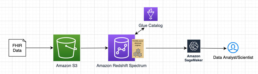
The following diagram illustrates the architecture of the solution.

In this post, we demonstrate how to use our open-source library with conjunction of Amazon Redshift PartiQL queries and Amazon Redshift Spectrum, which enables you to directly query and join data across your data warehouse and data lake. Our approach allows you to design a semi-relational schema, where scientists can quickly combine relational and non-relational data from multiple resource tables.

We use PartiQL in Amazon Redshift Spectrum over data stored in Amazon Simple Storage Service (Amazon S3). Amazon S3 is an object storage built to store and retrieve any amount of data, structured or unstructured, while providing extreme durability and availability, and infinitely scalable data storage infrastructure at very low costs. Amazon Redshift Spectrum runs complex SQL queries directly over Amazon S3 storage without loading or other data preparation, and AWS Glue serves as the meta-store catalog for the Amazon S3 data. That allows us to run PartiQL queries on Amazon S3 prefixes containing FHIR resources stored as JSON or Parquet files. We use Jupyter notebooks to illustrate how to build and use the Schema Induction tool, and for test data we use the public dataset from Fhirbase.

Querying FHIR using PartiQL

To provide a short introduction to PartiQL and illustrate the power of PartiQL, we show a few examples of PartiQL queries over FHIR data. Each example shows different aspects of query functionality varying from simple to aggregate queries. Although you can use this approach for myriad FHIR resources, we focus on claims data as an illustrative example. If you’re already familiar with PartiQL language, you can skip this section.

Assume that we have millions of claim documents as illustrated in claim-example-cms1500-medical.json and in the following code. We want to process attributes regarding ID (line 3), status (line 14), patient (lines 24–26), and diagnosis (lines 58–69):

1.	{
2.	  "resourceType": "Claim",
3.	  "id": "100150",
4.	  "text": {
5.	    "status": "generated",
6.	    "div": "<div xmlns=\"http://www.w3.org/1999/xhtml\">A human-readable rendering of the Oral Health Claim</div>"
7.	  },
8.	  "identifier": [
9.	    {
10.	      "system": "http://happyvalley.com/claim",
11.	      "value": "12345"
12.	    }
13.	  ],
14.	  "status": "active",
15.	  "type": {
16.	    "coding": [
17.	      {
18.	        "system": "http://terminology.hl7.org/CodeSystem/claim-type",
19.	        "code": "oral"
20.	      }
21.	    ]
22.	  },
23.	  "use": "claim",
24.	  "patient": {
25.	    "reference": "Patient/1"
26.	  },
27.	  "created": "2014-08-16",
28.	  "insurer": {
29.	    "reference": "Organization/2"
30.	  },
31.	  "provider": {
32.	    "reference": "Organization/1"
33.	  },
34.	  "priority": {
35.	    "coding": [
36.	      {
37.	        "code": "normal"
38.	      }
39.	    ]
40.	  },
41.	  "payee": {
42.	    "type": {
43.	      "coding": [
44.	        {
45.	          "code": "provider"
46.	        }
47.	      ]
48.	    }
49.	  },
50.	  "careTeam": [
51.	    {
52.	      "sequence": 1,
53.	      "provider": {
54.	        "reference": "Practitioner/example"
55.	      }
56.	    }
57.	  ],
58.	  "diagnosis": [
59.	    {
60.	      "sequence": 1,
61.	      "diagnosisCodeableConcept": {
62.	        "coding": [
63.	          {
64.	            "code": "123456"
65.	          }
66.	        ]
67.	      }
68.	    }
69.	  ],
70.	  "insurance": [
71.	    {
72.	      "sequence": 1,
73.	      "focal": true,
74.	      "identifier": {
75.	        "system": "http://happyvalley.com/claim",
76.	        "value": "12345"
77.	      },
78.	      "coverage": {
79.	        "reference": "Coverage/9876B1"
80.	      }
81.	    }
82.	  ],
83.	  "item": [
84.	    {
85.	      "sequence": 1,
86.	      "careTeamSequence": [
87.	        1
88.	      ],
89.	      "productOrService": {
90.	        "coding": [
91.	          {
92.	            "code": "1200"
93.	          }
94.	        ]
95.	      },
96.	      "servicedDate": "2014-08-16",
97.	      "unitPrice": {
98.	        "value": 135.57,
99.	        "currency": "USD"
100.	      },
101.	      "net": {
102.	        "value": 135.57,
103.	        "currency": "USD"
104.	      }
105.	    }
106.	  ]
107.	}

Creating the claims table DDL

To run queries with Amazon Redshift Spectrum, we first need to create the external table for the claims data. The claims table DDL must use special types such as Struct or Array with a nested structure to fit the structure of the JSON documents. For the FHIR claims document, we use the following DDL to describe the documents:

1.	  create external table fhir.Claims(
2.		"resourceType" varchar(500),
3.		"id" varchar(500),
4.		"status" varchar(500),
5.		"use" varchar(500),
6.		"patient" struct<"reference": varchar(500)>,
7.		"billablePeriod" struct<"start": varchar(500),"end": varchar(500)>,
8.		"organization" struct<"reference": varchar(500)>,
9.		"diagnosis" array<struct<"sequence": double precision,"diagnosisReference": struct<"reference": varchar(500)>>>,
10.		"item" array<struct<"sequence": double precision,"encounter": array<varchar(500)>,"diagnosisLinkId": array<double precision>,"informationLinkId": array<double precision>,"net": struct<"value": double precision,"system": varchar(500),"code": varchar(500)>,"procedureLinkId": array<double precision>>>,
11.		"total" struct<"value": double precision,"system": varchar(500),"code": varchar(500)>,
12.		"information" array<struct<"sequence": double precision,"category": struct<"coding": array<struct<"system": varchar(500),"code": varchar(500)>>>,"valueReference": struct<"reference": varchar(500)>>>,
13.		"procedure" array<struct<"sequence": double precision,"procedureReference": struct<"reference": varchar(500)>>>,
14.		"prescription" struct<"reference": varchar(500)>
15.	)
16.	row format serde 'org.openx.data.jsonserde.JsonSerDe'
17.	with serdeproperties ('dots.in.keys' = 'true','mapping.requesttime' = 'requesttimestamp','strip.outer.array' = 'true')
18.	location 's3://<bucket>/folder1/Claim-1/';

Because each column might be a highly nested JSON structure, this structure requires many levels of type definitions and optional attributes, as shown in lines 9–14. The definition of the preceding table works for a certain type of document in our sample. A table definition that can satisfy any claim document as defined by the FHIR JSON schema is even more complex. This is because the FHIR schema aims to capture any possible medical information, not just the existing data you have, and therefore is more complex than what you currently need.

Traditionally, creating a DDL table is a one-time operation performed by the database administrator, but devising DDL manually isn’t intuitive when it comes to a complex hierarchical dataset. Therefore, we created a new tool: the Schema Induction Tool, which is an open-source library that infers a schema out of a collection of documents and produces rich structure information of the collection of documents scanned.

Generating DDL with the Schema Induction Tool

The Schema Induction Tool is a java utility that reads a collection of JSON documents as stream, learns their common schema, and generates a create table statement for Amazon Redshift Spectrum. In addition, if the documents adhere to a JSON standard schema, the schema file can be provided for additional metadata annotations such as attributes descriptions, concrete datatypes, enumerations, and more. The JSON standard provides a comprehensive data structure for all possible variations of the data, whereas the enriched inferred schema only considers the structure that it has seen from the documents, and doesn’t explode the DDL statement with all the theoretical possibilities that the JSON schema defines. It is therefore imperative to provide a rich and heterogeneous set of documents that can provide the total possible paths in the current data. Because the utility uses stream processing, you can run it on a large volume of documents if time permits.

You can build the code yourself from the GitHub repo, or download a release artifact from Maven central.

The CLI syntax of the command is as follows:

java -jar aws-json-schema-induction.jar 
                        [-ah] [-c=<s3>] [-d=<outDdlFile>] -i=<inputFile> 
                        [-l=<tableLocation>] [-r=<region>] [-root=<rootDefinition>]
                        [-s=<outSchemaFile>] [--stats=<outStatsFile>]
                        [-t=<tableName>]
      -a, --array               is the document a json array
      -c, --cred=<s3>           which type of s3 credentials to use (ec2|profile)
      -d, --ddl=<outDdlFile>    An output ddl file for Redshift
      -h, --help                display a help message
      -i, --input=<inputFile>   An input json file path.
      -l, --location=<tableLocation>
                                table location to use when creating DDL
      -r, --region=<region>     s3 region to use
          -root, --root=<rootDefinition>
                                s3 region to use
      -s, --schema=<outSchemaFile>
                                An output schema file json file path
          --stats=<outStatsFile>
                                An output stats file
      -t, --table=<tableName>   table name to use when creating DDL 

The utility generates a DDL output file that contains the Create Table statement as defined by the ddl switch, and optionally a file that contains the hierarchical schema of the document collection as defined by the schema switch. Finally, a stat file is generated that contains the total number of occurrences of each element from the input documents collection.

Building the Induction Tool

We can now put it all together so we can analyze FHIR Claims data. We assume you have access to AWS account and also to a Linux terminal where you can access the data on Amazon S3 and run commands. We use Amazon SageMaker to host our Jupyter notebook.

  1. Build the Schema induction tool with the following code:
    git clone https://github.com/awslabs/amazon-redshift-json-schema-induction.git
    cd amazon-redshif-json-schema-induction
    mvn package

You use Amazon SageMaker to generate the Create Table statement for the claims.

  1. Create an Amazon SageMaker notebook on the Amazon SageMaker console.
  2. Select the notebook and choose Open JupyterLab.
  3. Copy the example data from your code folder schema-induction/target/schema-induction-1.0.0.jar to the notebook by dragging the file and dropping it into the left panel.
  4. Copy the example data from your code folder data/claims.json to the notebook.
  5. Copy the notebook document from your code folder notebooks/fhir-Partiql-notebook.ipynb.
  6. Open the notebook, set up the variables in the first cell per your account, and run the first cells to download and build the schema induction tool.

Preparing the data

Now the induction tool is ready and we can perform the schema induction.

  1. Run the next cells to download and check the test data.
  2. Check that the schema induction tool is ready and review the help guide.

Creating the FHIR table on Amazon Redshift

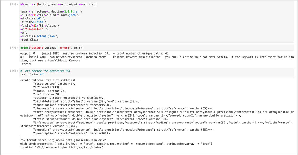
  1. Run the tool and review the induced DDL.

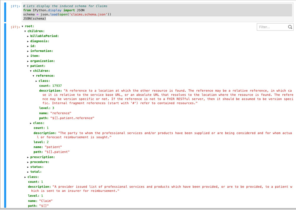
You can explore the data structure using the tree control display by running the following cell:

  1. On the AWS Glue console, create a database called fhir and leave location empty.
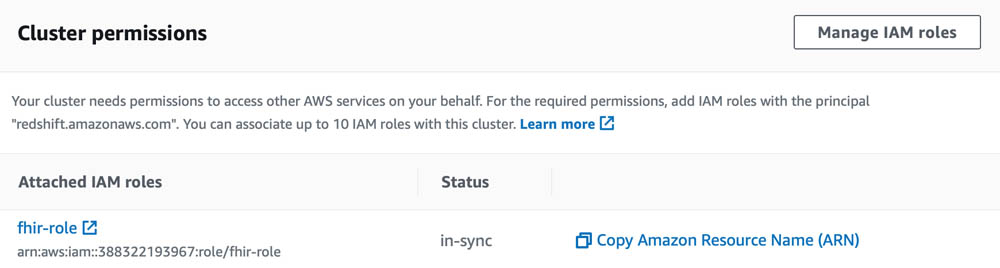
  2. Create an AWS Identity and Access Management (IAM) role that allows your Amazon Redshift cluster to access the S3 bucket and name it fhir-role.

For more information about creating an Amazon Redshift Spectrum role that can access your S3 buckets, see Authorizing Amazon Redshift to access other AWS services on your behalf.

  1. On your Amazon Redshift cluster, make sure you added the IAM role so you can run the queries and access Amazon S3 and AWS Glue and that the status shows as in-sync.

You can now run your PartiQL queries.

  1. Open the SQL Editor and connect to your database (in this use case, we use the Amazon Redshift Query Editor).
  2. Create the external schema in Amazon Redshift by entering the following code:
    create external schema fhir
    from data catalog
    database 'fhir'
    region '<your region>'
    iam_role 'arn:aws:iam::<account-id>:role/fhir-role';

For more information about creating external schema in Amazon Redshift, see CREATE EXTERNAL SCHEMA.

  1. Create the external table by copying the Create Table DDL from your notebook into your query and running it.
  2. Run your first PartiQL query on a new Query

Querying claims data

Claims are used by providers, payors, and insurers to exchange financial information and supporting clinical information regarding the provision of healthcare services with payors for reporting to regulatory bodies and firms that provide data analytics. In this section, we provide queries as examples of the analyses you can run.

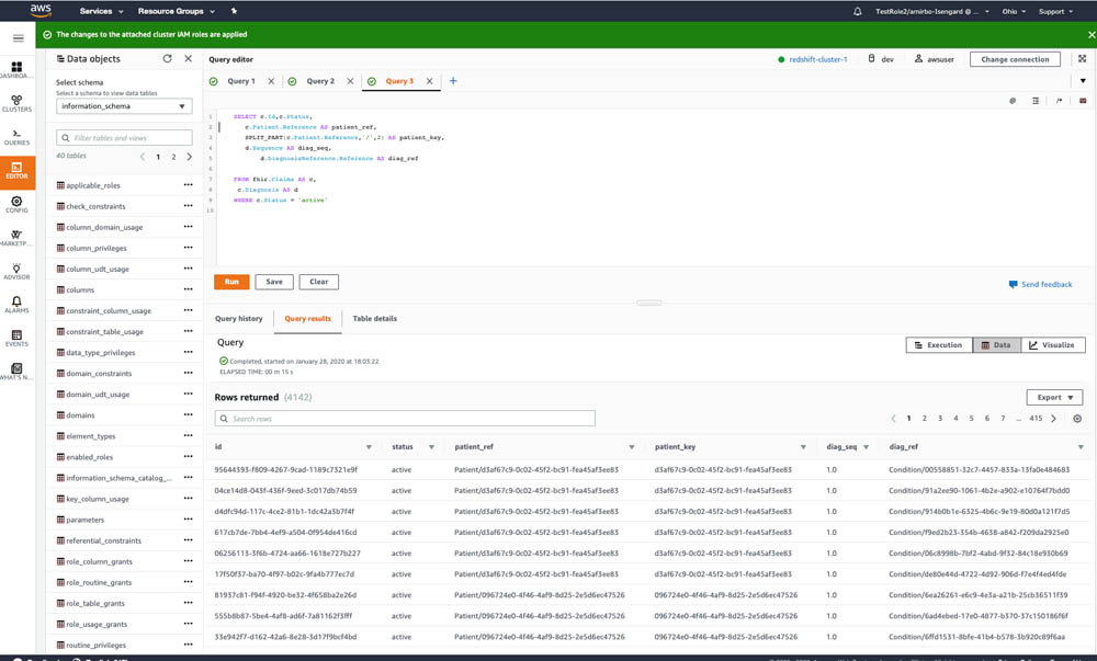
The following query scans all documents in the users.Claims table and retrieves information from each claim.

1.	SELECT c.id,c.status,
2.	       c.patient.reference as patient_ref, 
3.	       SPLIT_PART(c.patient.reference,'/',2) as patient_key,
4.	       d.sequence as diag_seq,
5.	       d.diagnosisReference.reference as diag_ref
6.	
7.	FROM fhir.Claims as c,
8.	     c.diagnosis as d
9.	WHERE c.status = 'active'  

The claim.diagnosis is an array that might contain multiple objects; it is therefore referenced in the SQL From clause and joined with the parent document implicitly, then attributes from the diagnosis element can be retrieved in the SELECT clause. This native SQL approach to un-nest arrays is one of the cornerstones of the PartiQL language. The query also uses the dot notation to access attributes in nested structures, such as c.patient.reference, which accesses the reference attribute inside the patient structure that is in the claim document.

Assuming there are claim documents without diagnosis information, and we want to retrieve the claims even if they have no diagnosis, we want a more permissive join by turning it into a left join. See the following code:

1.	SELECT c.id,c.status,
2.	       c.patient.reference as patient_ref, 
3.	       SPLIT_PART(c.patient.reference,'/',2) as patient_key,
4.	       d.sequence as diag_seq,
5.	       d.diagnosisReference.reference as diag_ref
6.	
7.	FROM fhir.Claims as c LEFT JOIN c.diagnosis as d
8.	WHERE c.status = 'active'  

You don’t need to specify the join keys because the join key is essentially the parent-child relationship of the claim and diagnosis structures.

The following query performs a simple aggregation over the claims data:

1.	SELECT c.status,count(*) as cnt, sum(c.total.value) as total
2.	FROM fhir.Claims as c
3.	GROUP BY c.status,c.patient.reference

It uses the c.patient.reference as the grouping key and the c.total.value as the aggregated value.

The following code queries all the patients’ claims:

1.	SELECT c.id,c.status,
2.	       c.patient.reference as patient_ref, 
3.	       SPLIT_PART(c.patient.reference,'/',2) as patient_key,
4.	       d.sequence as diag_seq,
5.	       d.diagnosisReference.reference as diag_ref
6.	
7.	FROM fhir.Claims as c,
8.	     c.diagnosis as d
9.	WHERE c.status = 'active'  

The following screenshot shows the query output.

Congratulations, you have successfully queried FHIR data in Amazon Redshift Spectrum using PartiQL language.

Conclusion

The FHIR standard looks promising to do great things for healthcare and although it has limitations, we believe the benefits are here to stay. You can directly analyze FHIR format without creating massive normalized design, and can leapfrog over competitors to save tremendous investments in data modeling and ETL maintenance. This post shows you the power of Amazon Redshift PartiQL and how your data science and data engineer team can handle complex data formats like FHIR easily with automation. Adopting these technologies can bring new innovation to the healthcare world and unlock new benefits and cost-optimization.

If you have any questions, please leave your thoughts in the comments section. We look forward to your feedback on our new open-source Schema Induction Tool in GitHub.


About the Authors

Amir Bar Or is a Principal Data Architect at AWS Professional Services. After 20 years leading software organizations and developing data analytics platforms and products, he is now sharing his experience with large enterprise customers and helping them scale their data analytics in the cloud.


Dr. Aaron Friedman a Principal Solutions Architect at Amazon Web Services working with healthcare and life sciences startups to accelerate science and improve patient care. His passion is working at the intersection of science, big data, and software. Outside of work, he’s with his family outdoors or learning a new thing to cook.


Crafting serverless streaming ETL jobs with AWS Glue

Post Syndicated from Radhika Ravirala original https://aws.amazon.com/blogs/big-data/crafting-serverless-streaming-etl-jobs-with-aws-glue/

Organizations across verticals have been building streaming-based extract, transform, and load (ETL) applications to more efficiently extract meaningful insights from their datasets. Although streaming ingest and stream processing frameworks have evolved over the past few years, there is now a surge in demand for building streaming pipelines that are completely serverless. Since 2017, AWS Glue has made it easy to prepare and load your data for analytics using ETL.

In this post, we dive into streaming ETL in AWS Glue, a feature that allows you to build continuous ETL applications on streaming data. Streaming ETL in AWS Glue is based on Apache Spark’s Structured Streaming engine, which provides a fault-tolerant, scalable, and easy way to achieve end-to-end stream processing with exactly-once semantics. This post walks you through an example of building a stream processing pipeline using AWS Glue that includes reading streaming data from Amazon Kinesis Data Streams, schema discovery, running streaming ETL, and writing out the results to a sink.

Serverless streaming ETL architecture

For this post, our use case is relevant to our current situation with the COVID-19 pandemic. Ventilators are in high demand and are increasingly used in different settings: hospitals, nursing homes, and even private residences. Ventilators generate data that must be monitored, and an increase in ventilator usage means there is a tremendous amount of streaming data that needs to be processed promptly, so patients can be attended to as quickly as possible as the need arises. In this post, we build a streaming ETL job on ventilator metrics and enhance the data with details to raise the alert level if the metrics fall outside of the normal range. After you enrich the data, you can use it to visualize on monitors.

In our streaming ETL architecture, a Python script generates sample ventilator metrics and publishes them as a stream into Kinesis Data Streams. We create a streaming ETL job in AWS Glue that consumes continuously generated ventilator metrics in micro-batches, applies transformations, performs aggregations, and delivers the data to a sink, so the results can be visualized or used in downstream processes.

Because businesses often augment their data lakes built on Amazon Simple Storage Service (Amazon S3) with streaming data, our first use case applies transformations on the streaming JSON data ingested via Kinesis Data Streams and loads the results in Parquet format to an Amazon S3 data lake. After ingested to Amazon S3, you can query the data with Amazon Athena and build visual dashboards using Amazon QuickSight.

For the second use case, we ingest the data from Kinesis Data Streams, join it with reference data in Amazon DynamoDB to calculate alert levels, and write the results to an Amazon DynamoDB sink. This approach allows you to build near real-time dashboards with alert notifications.

The following diagram illustrates this architecture.

AWS Glue streaming ETL jobs

With AWS Glue, you can now create ETL pipelines on streaming data using continuously running jobs. You can ingest streaming data from Kinesis Data Streams and Amazon Managed Streaming for Kafka (Amazon MSK). AWS Glue streaming jobs can perform aggregations on data in micro-batches and deliver the processed data to Amazon S3. You can read from the data stream and write to Amazon S3 using the AWS Glue DynamicFrame API. You can also write to arbitrary sinks using native Apache Spark Structured Streaming APIs.

The following sections walk you through building a streaming ETL job in AWS Glue.

Creating a Kinesis data stream

First, we need a streaming ingestion source to consume continuously generated streaming data. For this post, we create a Kinesis data stream with five shards, which allows us to push 5,000 records per second into the stream.

  1. On the Amazon Kinesis dashboard, choose Data streams.
  2. Choose Create data stream.
  3. For Data stream name, enter ventilatorsstream.
  4. For Number of open shards, choose 5.

If you prefer to use the AWS Command Line Interface (AWS CLI), you can create the stream with the following code:

aws kinesis create-stream \
    --stream-name ventilatorstream \
    --shard-count 5

Generating streaming data

We can synthetically generate ventilator data in JSON format using a simple Python application (see the GitHub repo) or the Kinesis Data Generator (KDG).

Using a Python-based data generator

To generate streaming data using a Python script, you can run the following command from your laptop or Amazon Elastic Compute Cloud (Amazon EC2) instance. Make sure you have installed the faker library on your system and set up the boto3 credentials correctly before you run the script.

python3 generate_data.py --streamname glue_ventilator_stream

Using the Kinesis Data Generator

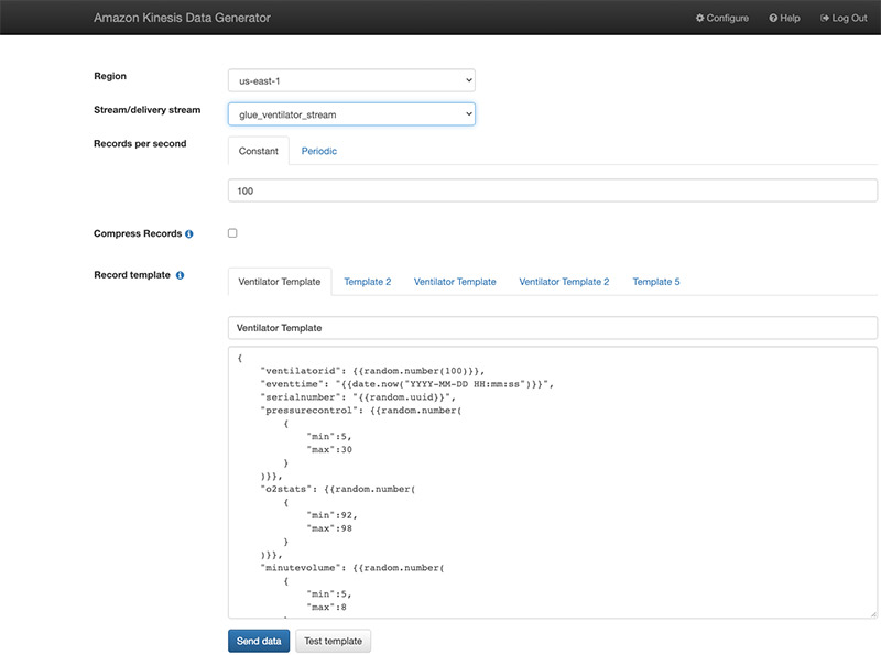
Alternatively, you can also use the Kinesis Data Generator with the ventilator template available on the GitHub repo. The following screenshot shows the template on the KDG console.

We start pushing the data after we create our AWS Glue streaming job.

Defining the schema

We need to specify a schema for our streaming data, which we can do one of two ways:

  • Retrieve a small batch of the data (before starting your streaming job) from the streaming source, infer the schema in batch mode, and use the extracted schema for your streaming job
  • Use the AWS Glue Data Catalog to manually create a table

For this post, we use the AWS Glue Data Catalog to create a ventilator schema.

  1. On the AWS Glue console, choose Data Catalog.
  2. Choose Tables.
  3. From the Add Table drop-down menu, choose Add table manually.
  4. For the table name, enter ventilators_table.
  5. Create a database with the name ventilatordb.
  6. Choose Kinesis as the type of source.
  7. Enter the name of the stream and https://kinesis.<aws-region>.amazonaws.com.
  8. For the classification, choose JSON.
  9. Define the schema according to the following table.
Column name Data type
ventilatorid int
eventtime string
serialnumber string
pressurecontrol int
o2stats int
minutevolume int
manufacturer string


  1. Choose Finish.

Creating an AWS Glue streaming job to hydrate a data lake on Amazon S3

With the streaming source and schema prepared, we’re now ready to create our AWS Glue streaming jobs. We first create a job to ingest data from the streaming source using AWS Glue DataFrame APIs.

  1. On the AWS Glue console, under ETL, choose Jobs.
  2. Choose Add job.
  3. For Name, enter a UTF-8 String with no more than 255 characters.
  4. For IAM role¸ specify a role that is used for authorization to resources used to run the job and access data stores. Because streaming jobs require connecting to sources and sinks, you need to make sure that the AWS Identity and Access Management (IAM) role has permissions to read from Kinesis Data Stream, write to Amazon S3 and read, write to Amazon DynamoDB. Refer to Managing Access Permissions for AWS Glue Resources for details.
  5. For Type, choose Spark Streaming.
  6. For Glue Version, choose Spark 2.4, Python 3.
  7. For This job runs, select A new script authored by you.

You can have AWS Glue generate the streaming ETL code for you, but for this post, we author one from scratch.

  1. For Script file name, enter GlueStreaming-S3.
  2. For S3 path where script is stored, enter your S3 path.
  3. For Job bookmark, choose Disable.

For this post, we use the checkpointing mechanism of AWS Glue to keep track of the data read instead of a job bookmark.

  1. For Monitoring options, select Job metrics and Continuous logging.
  2. For Log filtering, select Standard filter and Spark UI.
  3. For Amazon S3 prefix for Spark event logs, enter the S3 path for the event logs.
  4. For Job parameters, enter the following key-values:
    1. –output path – The S3 path where the final aggregations are persisted
    2. –aws_region – The Region where you run the job

  5. Skip the connections part and choose Save and edit the script.

Streaming ETL to an Amazon S3 sink

We use the AWS Glue DynamicFrameReader class’s from_catalog method to read the streaming data. We specify the table name that has been associated with the data stream as the source of data (see the section Defining the schema). We add additional_options to indicate the starting position to read from in Kinesis Data Streams. TRIM_HORIZON allows us to start reading from the oldest record in the shard.

# Read from Kinesis Data Stream
sourceData = glueContext.create_data_frame.from_catalog( \
    database = "ventilatordb", \
    table_name = "ventilatortable", \
    transformation_ctx = "datasource0", \
    additional_options = {"startingPosition": "TRIM_HORIZON", "inferSchema": "true"})

In the preceding code, sourceData represents a streaming DataFrame. We use the foreachBatch API to invoke a function (processBatch) that processes the data represented by this streaming DataFrame. The processBatch function receives a static DataFrame, which holds streaming data for a window size of 100s (default). It creates a DynamicFrame from the static DataFrame and writes out partitioned data to Amazon S3. See the following code:

glueContext.forEachBatch(frame = sourceData, batch_function = processBatch, options = {"windowSize": "100 seconds", "checkpoint_locationation": checkpoint_location})

To transform the DynamicFrame to fix the data type for eventtime (from string to timestamp) and write the ventilator metrics to Amazon S3 in Parquet format, enter the following code:

def processBatch(data_frame, batchId):
    now = datetime.datetime.now()
    year = now.year
    month = now.month
    day = now.day
    hour = now.hour
    minute = now.minute
    if (data_frame.count() > 0):
        dynamic_frame = DynamicFrame.fromDF(data_frame, glueContext, "from_data_frame")
        apply_mapping = ApplyMapping.apply(frame = dynamic_frame, mappings = [ \
            ("ventilatorid", "long", "ventilatorid", "long"), \
            ("eventtime", "string", "eventtime", "timestamp"), \
            ("serialnumber", "string", "serialnumber", "string"), \
            ("pressurecontrol", "long", "pressurecontrol", "long"), \
            ("o2stats", "long", "o2stats", "long"), \
            ("minutevolume", "long", "minutevolume", "long"), \
            ("manufacturer", "string", "manufacturer", "string")],\
            transformation_ctx = "apply_mapping")

        dynamic_frame.printSchema()

        # Write to S3 Sink
        s3path = s3_target + "/ingest_year=" + "{:0>4}".format(str(year)) + "/ingest_month=" + "{:0>2}".format(str(month)) + "/ingest_day=" + "{:0>2}".format(str(day)) + "/ingest_hour=" + "{:0>2}".format(str(hour)) + "/"
        s3sink = glueContext.write_dynamic_frame.from_options(frame = apply_mapping, connection_type = "s3", connection_options = {"path": s3path}, format = "parquet", transformation_ctx = "s3sink")

Putting it all together

In the Glue ETL code editor, enter the following code, then save and run the job:

import sys
import datetime
import boto3
import base64
from pyspark.sql import DataFrame, Row
from pyspark.context import SparkContext
from pyspark.sql.types import *
from pyspark.sql.functions import *
from awsglue.transforms import *
from awsglue.utils import getResolvedOptions
from awsglue.context import GlueContext
from awsglue.job import Job
from awsglue import DynamicFrame

args = getResolvedOptions(sys.argv, \
                            ['JOB_NAME', \
                            'aws_region', \
                            'output_path'])

sc = SparkContext()
glueContext = GlueContext(sc)
spark = glueContext.spark_session
job = Job(glueContext)
job.init(args['JOB_NAME'], args)

# S3 sink locations
aws_region = args['aws_region']
output_path = args['output_path']

s3_target = output_path + "ventilator_metrics"
checkpoint_location = output_path + "cp/"
temp_path = output_path + "temp/"


def processBatch(data_frame, batchId):
    now = datetime.datetime.now()
    year = now.year
    month = now.month
    day = now.day
    hour = now.hour
    minute = now.minute
    if (data_frame.count() > 0):
        dynamic_frame = DynamicFrame.fromDF(data_frame, glueContext, "from_data_frame")
        apply_mapping = ApplyMapping.apply(frame = dynamic_frame, mappings = [ \
            ("ventilatorid", "long", "ventilatorid", "long"), \
            ("eventtime", "string", "eventtime", "timestamp"), \
            ("serialnumber", "string", "serialnumber", "string"), \
            ("pressurecontrol", "long", "pressurecontrol", "long"), \
            ("o2stats", "long", "o2stats", "long"), \
            ("minutevolume", "long", "minutevolume", "long"), \
            ("manufacturer", "string", "manufacturer", "string")],\
            transformation_ctx = "apply_mapping")

        dynamic_frame.printSchema()

        # Write to S3 Sink
        s3path = s3_target + "/ingest_year=" + "{:0>4}".format(str(year)) + "/ingest_month=" + "{:0>2}".format(str(month)) + "/ingest_day=" + "{:0>2}".format(str(day)) + "/ingest_hour=" + "{:0>2}".format(str(hour)) + "/"
        s3sink = glueContext.write_dynamic_frame.from_options(frame = apply_mapping, connection_type = "s3", connection_options = {"path": s3path}, format = "parquet", transformation_ctx = "s3sink")

# Read from Kinesis Data Stream
sourceData = glueContext.create_data_frame.from_catalog( \
    database = "ventilatordb", \
    table_name = "ventilatortable", \
    transformation_ctx = "datasource0", \
    additional_options = {"startingPosition": "TRIM_HORIZON", "inferSchema": "true"})

sourceData.printSchema()

glueContext.forEachBatch(frame = sourceData, batch_function = processBatch, options = {"windowSize": "100 seconds", "checkpoint_locationation": checkpoint_location})
job.commit()

Querying with Athena

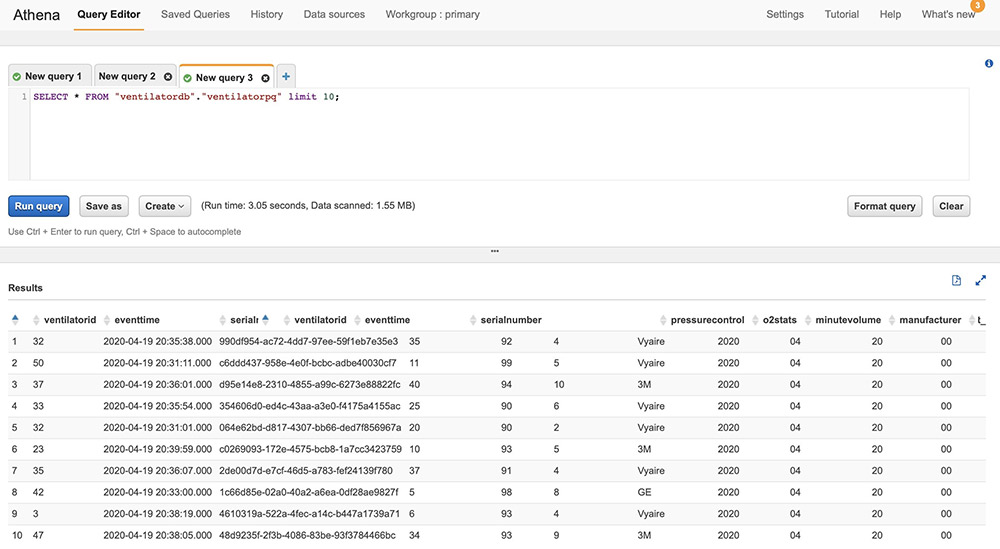
When the processed streaming data is written in Parquet format to Amazon S3, we can run queries on Athena. Run the AWS Glue crawler on the Amazon S3 location where the streaming data is written out. The following screenshot shows our query results.

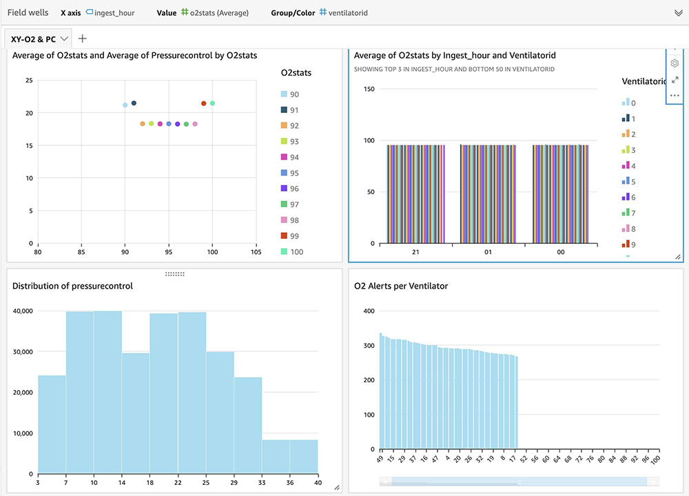
For instructions on building visual dashboards with the streaming data in Amazon S3, see Quick Start: Create an Analysis with a Single Visual Using Sample Data. The following dashboards show distribution of metrics, averages, and alerts based on anomalies on an hourly basis, but you can create more advanced dashboards with much granular (minute) intervals.

Streaming ETL to a DynamoDB sink

For the second use case, we transform the streaming data as it arrives without micro-batching and persist the data to a DynamoDB table. Scripts to create DynamoDB tables are available in the GitHub repo. We use Apache Spark’s Structured Streaming API to read ventilator-generated data from the data stream, join it with reference data for normal metrics range in a DynamoDB table, compute the status based on the deviation from normal metric values, and write the processed data to a DynamoDB table. See the following code:

import sys
import datetime
import base64
import decimal
import boto3
from pyspark.sql import DataFrame, Row
from pyspark.context import SparkContext
from pyspark.sql.types import *
from pyspark.sql.functions import *
from awsglue.transforms import *
from awsglue.utils import getResolvedOptions
from awsglue.context import GlueContext
from awsglue.job import Job
from awsglue import DynamicFrame

args = getResolvedOptions(sys.argv, \
                            ['JOB_NAME', \
                            'aws_region', \
                            'checkpoint_location', \
                            'dynamodb_sink_table', \
                            'dynamodb_static_table'])

sc = SparkContext()
glueContext = GlueContext(sc)
spark = glueContext.spark_session
job = Job(glueContext)
job.init(args['JOB_NAME'], args)

# Read parameters
checkpoint_location = args['checkpoint_location']
aws_region = args['aws_region']

# DynamoDB config
dynamodb_sink_table = args['dynamodb_sink_table']
dynamodb_static_table = args['dynamodb_static_table']

def write_to_dynamodb(row):
    '''
    Add row to DynamoDB.
    '''
    dynamodb = boto3.resource('dynamodb', region_name=aws_region)
    start = str(row['window'].start)
    end = str(row['window'].end)
    dynamodb.Table(dynamodb_sink_table).put_item(
      Item = { 'ventilatorid': row['ventilatorid'], \
                'status': str(row['status']), \
                'start': start, \
                'end': end, \
                'avg_o2stats': decimal.Decimal(str(row['avg_o2stats'])), \
                'avg_pressurecontrol': decimal.Decimal(str(row['avg_pressurecontrol'])), \
                'avg_minutevolume': decimal.Decimal(str(row['avg_minutevolume']))})

dynamodb_dynamic_frame = glueContext.create_dynamic_frame.from_options( \
    "dynamodb", \
    connection_options={
    "dynamodb.input.tableName": dynamodb_static_table,
    "dynamodb.throughput.read.percent": "1.5"
  }
)

dynamodb_lookup_df = dynamodb_dynamic_frame.toDF().cache()

# Read from Kinesis Data Stream
streaming_data = spark.readStream \
                    .format("kinesis") \
                    .option("streamName","glue_ventilator_stream") \
                    .option("endpointUrl", "https://kinesis.us-east-1.amazonaws.com") \
                    .option("startingPosition", "TRIM_HORIZON") \
                    .load()

# Retrieve Sensor columns and do a simple projection
ventilator_fields = streaming_data \
    .select(from_json(col("data") \
    .cast("string"),glueContext.get_catalog_schema_as_spark_schema("ventilatordb","ventilators_table")) \
    .alias("ventilatordata")) \
    .select("ventilatordata.*") \
    .withColumn("event_time", to_timestamp(col('eventtime'), "yyyy-MM-dd HH:mm:ss")) \
    .withColumn("ts", to_timestamp(current_timestamp(), "yyyy-MM-dd HH:mm:ss"))

# Stream static join, ETL to augment with status
ventilator_joined_df = ventilator_fields.join(dynamodb_lookup_df, "ventilatorid") \
    .withColumn('status', when( \
    ((ventilator_fields.o2stats < dynamodb_lookup_df.o2_stats_min) | \
    (ventilator_fields.o2stats > dynamodb_lookup_df.o2_stats_max)) & \
    ((ventilator_fields.pressurecontrol < dynamodb_lookup_df.pressure_control_min) | \
    (ventilator_fields.pressurecontrol > dynamodb_lookup_df.pressure_control_max)) & \
    ((ventilator_fields.minutevolume < dynamodb_lookup_df.minute_volume_min) | \
    (ventilator_fields.minutevolume > dynamodb_lookup_df.minute_volume_max)), "RED") \
    .when( \
    ((ventilator_fields.o2stats >= dynamodb_lookup_df.o2_stats_min) |
    (ventilator_fields.o2stats <= dynamodb_lookup_df.o2_stats_max)) & \
    ((ventilator_fields.pressurecontrol >= dynamodb_lookup_df.pressure_control_min) | \
    (ventilator_fields.pressurecontrol <= dynamodb_lookup_df.pressure_control_max)) & \
    ((ventilator_fields.minutevolume >= dynamodb_lookup_df.minute_volume_min) | \
    (ventilator_fields.minutevolume <= dynamodb_lookup_df.minute_volume_max)), "GREEN") \
    .otherwise("ORANGE"))

ventilator_joined_df.printSchema()

# Drop the normal metric values
ventilator_transformed_df = ventilator_joined_df \
                            .drop('eventtime', 'o2_stats_min', 'o2_stats_max', \
                            'pressure_control_min', 'pressure_control_max', \
                            'minute_volume_min', 'minute_volume_max')

ventilator_transformed_df.printSchema()

ventilators_df = ventilator_transformed_df \
    .groupBy(window(col('ts'), '10 minute', '5 minute'), \
    ventilator_transformed_df.status, ventilator_transformed_df.ventilatorid) \
    .agg( \
    avg(col('o2stats')).alias('avg_o2stats'), \
    avg(col('pressurecontrol')).alias('avg_pressurecontrol'), \
    avg(col('minutevolume')).alias('avg_minutevolume') \
    )

ventilators_df.printSchema()

# Write to DynamoDB sink
ventilator_query = ventilators_df \
    .writeStream \
    .foreach(write_to_dynamodb) \
    .outputMode("update") \
    .option("checkpointLocation", checkpoint_location) \
    .start()

ventilator_query.awaitTermination()

job.commit()

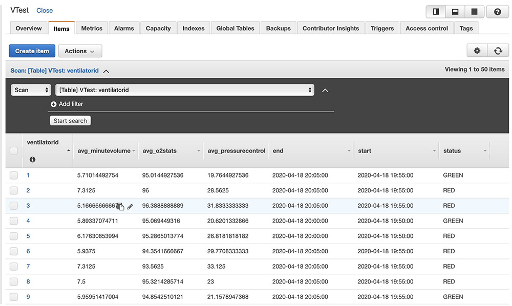
After the above code is run, ventilator metric aggregations get persisted in the Amazon DynamoDB table as follows. You can build custom user interface applications with the data in Amazon DynamoDB to create dashboards.

Conclusion

Streaming applications have become a core component of data lake architectures. With AWS Glue streaming, you can create serverless ETL jobs that run continuously, consuming data from streaming services like Kinesis Data Streams and Amazon MSK. You can load the results of streaming processing into an Amazon S3-based data lake, JDBC data stores, or arbitrary sinks using the Structured Streaming API.

For more information about streaming AWS Glue ETL jobs, see the following:

We encourage you to build a serverless streaming application using AWS Glue streaming ETL and share your experience with us. If you have any questions or suggestions, share them in the comments.


About the Author


Radhika Ravirala is a specialist solutions architect at Amazon Web Services, where she helps customers craft distributed analytics applications on the AWS platform. Prior to her cloud journey, she worked as a software engineer and designer for technology companies in Silicon Valley.

Automating EMR workloads using AWS Step Functions

Post Syndicated from Afsar Jahangir original https://aws.amazon.com/blogs/big-data/automating-emr-workloads-using-aws-step-functions/

Amazon EMR allows you to process vast amounts of data quickly and cost-effectively at scale. Using open-source tools such as Apache Spark, Apache Hive, and Presto, and coupled with the scalable storage of Amazon Simple Storage Service (Amazon S3), Amazon EMR gives analytical teams the engines and elasticity to run petabyte-scale analysis for a fraction of the cost of traditional on-premises clusters. Developers and analysts can use Jupyter-based Amazon EMR notebooks for iterative development, collaboration, and access to data stored across AWS data products.

What happens if you have Amazon EMR code that needs to run automatically on a regular basis? Maybe the job only runs when for certain events, like new data arriving in Amazon S3. Or maybe you want to run a job every Friday afternoon at 2:00 PM. What if there is a multiple step process?

To run Amazon EMR workloads on a schedule, you can automate everything with AWS Step Functions. This post walks through how to use Step Functions state machines and the callback pattern to automate EMR jobs. You can download the code examples from the GitHub repo.

Prerequisites

To follow along with this walkthrough, you must have the following:

Solution overview

For this use case, I want to run two applications on my EMR cluster. The start of the second application depends on the successful completion and output of the first. At a high level, I want to launch an EMR cluster automatically, run the code, and remove the cluster. Specifically, when the first program successfully completes, I want to run the second program.

At the conclusion of the second application, in some cases I may want to run both programs multiple times (with different dataset sizes, perhaps). I need a way to decide to run the process again with the same cluster. Whether the steps succeed or fail, at the conclusion, I always want to delete the CloudFormation stack that contains my EMR cluster to reduce cost. The following diagram illustrates this high-level overview of the pipeline operation.

Workflow details

I run two programs, and I need the first program to complete before running the second one. I optionally want to repeat those two programs with different datasets to get the final state of the data. To orchestrate the jobs, I can run through the same steps multiple times with the same active EMR cluster.

To facilitate automating the pipeline, I use an inner state machine to check the cluster status and submit EMR job steps. I then wrap that inner state machine in an outer state machine. The outer state machine starts the cluster and submits information to the inner state machine. It waits for all steps to complete, then deletes the EMR cluster.

The following flow chart illustrates the steps and checkpoints that make up the pipeline.

Deploying the pipeline state machines

To simplify pipeline deployment, I use AWS SAM, an open-source framework for building serverless applications. AWS SAM provides a single deployment configuration, extensions to CloudFormation templates, built-in best practices, and local debugging and testing. You can use AWS SAM with a suite of AWS tools for building serverless applications. For more information, see What Is the AWS Serverless Application Model (AWS SAM)?

Initiating the application

Navigate to the path where you want to download the files and initiate the AWS SAM application. I want to run the code from my local machine and have created the following location:

~/Documents/projects/blog/steppipeline/automation-ml-step-data-pipeline

From this directory, I initialize the application using sam init. This connects to the repository and downloads the files for creation of the ML pipeline. See the following code:

sam init -l https://github.com/aws-samples/automation-ml-step-data-pipeline.git

Creating the S3 bucket and moving dependencies

For this post, I orchestrate an existing process from the post Anomaly Detection Using PySpark, Hive, and Hue on Amazon EMR, which runs on Amazon EMR. The pipeline reads code artifacts from Amazon S3, where the EMR cluster has read permission. There are two programs: kmeansandey.py and kmeanswsssey.py.

First, create the bucket from the command line using the aws s3 mb command and upload the code. Your bucket name must be globally unique:

aws s3 mb s3://<your bucket name>

Move the artifacts to your bucket, replacing <your bucket name> with your bucket name:

aws s3 cp sample_ml_code/kmeansandey.py s3://<your bucket name>/testcode/kmeansandey.py
aws s3 cp sample_ml_code/kmeanswsssey.py s3://<your bucket name>/testcode/kmeanswsssey.py
aws s3 cp emr/bootstrapactions.sh s3://<your bucket name>/emr-bootstrap-scripts/bootstrapactions.sh
aws s3 cp emr/emr-cluster-config.json s3://<your bucket name>/emr-cluster-config.json
aws s3 cp emr/emr-cluster-sample.yaml s3://<your bucket name>/emr-cluster-sample.yaml

Deploying the application

Deploy the build artifacts to the AWS Cloud using the following code:

sam deploy --guided

AWS SAM prompts you for the parameters that you need to build and deploy the application. I have provided some default values where possible.

The final output of your deployment process should indicate that all stacks were built:

Successfully created/updated stack - step-pipeline in us-east-1

After deployment, you receive an email to confirm your subscription. Choose the confirmation link in the email to receive pipeline notifications.

Submitting a workload to your Step Functions state machine

To create a cluster and submit EMR jobs, the outer state machine needs a JSON payload. This contains the location of the programs in Amazon S3, the Amazon EMR CloudFormation template, and the parameter files used to launch the EMR cluster.

Creating an Amazon EC2 key pair

To use the same sample programs and EMR cluster template that you used to test your pipeline, you need to use an Amazon EC2 key pair for SSH credentials. When you create a cluster, you can specify the Amazon Elastic Compute Cloud (Amazon EC2) key pair to use for SSH connections to all cluster instances. The name of the keypair for this cluster is referenced in the emr-cluster-config.json file. See the following code:

<snip>
  {
    "ParameterKey": "Keyname",
    "ParameterValue": "emrcluster-launch"
  },
</snip>

To use the example as-is with the parameters unchanged, create an Amazon EC2 key pair on the AWS Management Console or AWS Command Line Interface (AWS CLI).

  1. On the Amazon EC2 console, under Network & Security, choose Key Pairs.
  2. On the Key Pairs page, choose Create Key Pair.
  3. For Key pair name, enter emrcluster-launch.
  4. Choose Create.
  5. When the console prompts you to save the private key file, save it in a safe place.

This is the only chance for you to save the private key file.

Inputting JSON for launching the pipeline

The simplest way for you to run the pipeline is to use the Start execution feature on the Step Functions console. The console gives you full functionality to initiate the function and submit a payload. In the example test_input.json, update the bucket values, security group, and subnet with the information for your account:

{  
    "ModelName": "PipelineTest_01",  
    "ModelProgram": "s3://<your bucket name>/testcode/kmeansandey.py",  
    "PreProcessingProgram": "s3://<your bucket name>/testcode/kmeanswsssey.py",  
    "EMRCloudFormation": "https://s3.amazonaws.com/<your bucket name>/emr-cluster-sample.yaml",  
    "EMRParameters": "https://s3.amazonaws.com/<your bucket name>/emr-cluster-config.json",  
    "JobInput": "s3://aws-bigdata-blog/artifacts/anomaly-detection-using-pyspark/sensorinputsmall/",  
    "SecurityGroup": "<your security group>",  
    "SubNet": "<your subnet>",  
    "ClusterSize": "4",  
    "ProcessingMode": ["TRAINING"]
}

The payload includes the following information:

  • ModelName – A short descriptive identifier used to identify the transient EMR cluster created during this process. This name shows on the Amazon EMR console for easy identification.
  • ModelProgram – The Amazon S3 URL location of the program that runs when the model initiates on the EMR cluster (step 3).
  • PreProcessingProgram – The Amazon S3 URL location of the program that runs when preprocessing initiates on the EMR cluster (step 2).
  • EMRCloudFormation – The S3 bucket HTTPS location of the CloudFormation template for launching the transient EMR cluster.
  • EMRParameters – The Amazon S3 HTTPS location of the parameter file supporting the Amazon EMR CloudFormation template.
  • JobInput – The Amazon S3 URL location of the input data for the preprocessing program.
  • SecurityGroup – The security group with ingress and egress rules for the launched EMR cluster
  • SubNet – The subnet identifier where you place your EMR cluster.
  • ClusterSize – Denotes the number of EMR cluster nodes to run the job and can be changed based on the compute need. I use 4 nodes as the input value for the sample program.
  • ProcessingMode – This is an array of values. The pipeline runs steps 2 and 3 for each value in the array. The value is passed into the program unchanged and can be used to internally control how the program runs. For this use case, it runs a single time on the small dataset.

Opening the Step Functions Executions page

On the Step Functions console, choose MLStateMachine. This is the outer state machine. On the detail page for the outer state machine, choose Start execution.

Entering your payload

On the New execution page, enter the JSON for your pipeline based on the example test_input.json. Choose Start execution.

Reviewing the workflow as it runs

You can see the pipeline running in the visual workflow and review the event history on the detail page. The following diagram shows the state machine definition used:

Diving into the pipelines details

There are four processes that run in the outer state machine pipeline:

  1. Step 1 launches an EMR cluster using the CloudFormation template. The AWS Lambda function downloads the template and parameter file from the specified Amazon S3 location and initiates the stack build.
  2. When the EMR cluster is ready, step 2 initiates the first set of code against the newly created EMR cluster, passing in the remaining parameters to the inner state machine. It adds the stack id, EMR cluster id, and status to the payload. These values are obtained from the output of the CloudFormation stack. See the following code:
    "ModelName": "PipelineTest_01",  
    "PreProcessingProgram": "s3://<your bucket name>/testcode/kmeanswsssey.py",  
    "JobInput": "s3://aws-bigdata-blog/artifacts/anomaly-detection-using-pyspark/sensorinputsmall/",  
    "ClusterSize": "4",  
    "ProcessingMode": ["TRAINING"],
    "StackId": "arn:aws:cloudformation:us-east-1:575444587305:stack/PipelineTest01-auto-emr-02142020041612/bc5fd7a0-4ee0-11ea-a395-0e4c53e0aefd",
    "Status": "CREATE_COMPLETE",
    "ClusterId": "j-MF6LWBLJZ88K"

The code contains the following information:

  • ModelName is used in the EMR cluster name to make it easier to identify in the console and AWS CLI output.
  • PreProcessingProgram in our use case points to the first code step (py). The code is passed through the first state machine and submitted to the second state machine and Amazon EMR.
  • JobInput, ClusterSize, ClusterId, StackId, and ProcessingMode are passthrough values that the program needs to run.

The step initiates the Lambda function awsblog-testproject-inner-sm-AddStepLambda-x45123xxxxxx, which engages the inner state machine asynchronously to run a high-level process of checking the cluster, adding a step, checking to see if the step is complete, and exiting back to the outer state machine when complete.

  1. Next, the outer state machine runs the Model program code (step 3) by submitting it to the Lambda function awsblog-testproject-inner-sm-AddStepLambda-x45123xxxxxx to engage the inner state machine for the second set of code (py). The process is the same as step 2 but the code it runs is from a different file and the output from the preprocessing step becomes the input for the step. See the following code:
    "ModelProgram": "s3://<your bucket name>/testcode/kmeansandey.py",

When the inner state machine is complete, it moves to a step that removes the first value from the ProcessingMode array. For this use case, there is only one value (TRAINING), which is removed, leaving the array empty. The next step in the state machine looks for remaining values; if there are none, it marks all steps as complete and moves to Delete EMR cluster.

  1. The final step in the outer state machine is to remove the EMR cluster. The Delete EMR cluster step passes the CloudFormation stack ID into lambda/delete_cfn_stack.py, initiating the deletion of the stack and cleaning up all the resources.

The output of the test programs is stored in Amazon S3 in two folders under the pipeline artifacts. The preprocessing folder contains data that is used to drive the output in the model folder. The following screenshot shows the folders in Amazon S3.

Conclusion

The Step Functions workflow in this post is a repeatable two-step pipeline. It starts an EMR cluster, runs a program that outputs data, and initiates a second program that depends on the previous job finishing. It then deletes all resources automatically.

You can adapt the workflow to respond to Amazon S3 events, a message received in a queue, a file checked into a code repository, or a schedule. Any event that can invoke Lambda can initiate the pipeline. For more information, see Invoking AWS Lambda functions.

You can download the example code from the GitHub repo and adapt it for your use case. Let me know in the comments what you built for your environment.


About the Authors

Mohammed “Afsar ” Jahangir Ali is a Senior Big Data Consultant with Amazon since January 2018. He is a data enthusiast helping customers shape their data lakes and analytic journeys on AWS.In his spare time, he enjoys taking pictures, listening to music, and spend time with family.


Wendy Neu has worked as a Data Architect with Amazon since January 2015. Prior to joining Amazon, she worked as a consultant in Cincinnati, OH helping customers integrate and manage their data from different unrelated data sources.


Event-driven refresh of SPICE datasets in Amazon QuickSight

Post Syndicated from Dylan Qu original https://aws.amazon.com/blogs/big-data/event-driven-refresh-of-spice-datasets-in-amazon-quicksight/

Businesses are increasingly harnessing data to improve their business outcomes. To enable this transformation to a data-driven business, customers are bringing together data from structured and unstructured sources into a data lake. Then they use business intelligence (BI) tools, such as Amazon QuickSight, to unlock insights from this data.

To provide fast access to datasets, QuickSight provides a fully managed calculation engine called SPICE—the Super-fast, Parallel, In-Memory Calculation Engine. At the time of writing, SPICE enables you to cache up to 250 million rows or 500 GB of data per dataset.

To extract value from the data quickly, you need access to new data as soon as it’s available. In this post, we describe how to achieve this by refreshing SPICE datasets as part of your extract, transform, and load (ETL) pipelines.

Solution architecture

In this post, you automate the refresh of SPICE datasets by implementing the following architecture.

This architecture consists of two parts: an example ETL job and a decoupled event-driven process to refresh SPICE.

For the ETL job, you use Amazon Simple Storage Service (Amazon S3) as your primary data store. Data lands in an S3 bucket, which we refer to as the raw zone. An Amazon S3 trigger configured on this bucket triggers an AWS Lambda function, which starts an AWS Glue ETL job. This job processes the raw data and outputs processed data into another S3 bucket, which we refer to as the processed zone.

This sample ETL job converts the data to Apache Parquet format and stores it in the processed S3 bucket. You can modify the ETL job to achieve other objectives, like more granular partitioning, compression, or enriching of the data. The Glue Data Catalog stores the metadata and QuickSight datasets are created using Amazon Athena data sources.

To trigger the SPICE dataset refresh, after the ETL job finishes, an Amazon EventBridge rule triggers a Lambda function that initiates the refresh.

In summary, this pipeline transforms your data and updates QuickSight SPICE datasets upon completion.

Deploying the automated data pipeline using AWS CloudFormation

Before deploying the AWS CloudFormation template, make sure you have signed up for QuickSight in one of the 11 supported Regions:

  • US East (Ohio)
  • US East (N. Virginia)
  • US West (Oregon)
  • Asia Pacific (Mumbai)
  • Asia Pacific (Seoul)
  • Asia Pacific (Singapore)
  • Asia Pacific (Sydney)
  • Asia Pacific (Tokyo)
  • EU (Frankfurt)
  • EU (Ireland)
  • EU (London)

This post works with both Standard and Enterprise editions of QuickSight. Enterprise Edition provides richer features and higher limits compared to Standard Edition.

  1. After you sign up for QuickSight, you can use CloudFormation templates to create all the necessary resources by choosing Launch stack:
  2. Enter a stack name; for example, SpiceRefreshBlog.
  3. Acknowledge the AWS Identity and Access Management (IAM) resource creation.
  4. Choose Create stack.

The CloudFormation template creates the following resources in your AWS account:

  • Three S3 buckets to store the following:
    • AWS Glue ETL job script
    • Raw data
    • Processed data
  • Three Lambda functions to do the following:
    • Create the ETL job
    • Initiate the ETL job upon upload of new data in the raw zone
    • Initiate the SPICE dataset refresh when the ETL job is complete
  • An AWS Glue database
  • Two AWS Glue tables to store the following:
    • Raw data
    • Processed data
  • An ETL job to convert the raw data from CSV into Apache Parquet format
  • Four IAM roles: One each for the Lambda functions and one for the ETL job
  • An EventBridge rule that triggers on an AWS Glue job state change event with a state of Succeeded and invokes a Lambda function that performs the SPICE dataset refresh

Importing the dataset

For this post, you use the taxi Trip Record Data dataset publicly available from the NYC Taxi & Limousine Commission Trip Record Data dataset. You upload monthly data in CSV format to the raw zone S3 bucket.

This data is available in Amazon S3 through Open Data on AWS, a service designed to let you spend more time on data analysis rather than data acquisition.

You start by copying the For Hire Vehicle (FHV) data for March 2020. Because the data is already available in Amazon S3 through Open Data, run the following command to copy the data into the raw zone. Make sure you replace <raw bucket name> with the name of the raw bucket created by the CloudFormation template:

aws s3 cp "s3://nyc-tlc/trip data/fhv_tripdata_2020-03.csv" s3://<raw bucket name>

After you copy the data into the raw zone, the Amazon S3 event trigger invokes the Lambda function that triggers the ETL job. You can see the job status on the AWS Glue console by choosing Jobs in the navigation pane. The process takes about 2 minutes.

When the job is complete, check that you can see the Parquet files in the processed zone S3 bucket.

Creating a QuickSight analysis of the data

To visualize the taxi data, we create a QuickSight analysis.

First, you need to give QuickSight the necessary permissions to access the processed zone S3 bucket. For instructions, see I Can’t Connect to Amazon S3.

Then complete the following steps to create an analysis of the taxi data:

  1. On the QuickSight console, choose Datasets.
  2. Choose New dataset.
  3. Choose Athena and provide a name for the data source (such as Athena).
  4. Choose Create data source.
  5. For Database, choose the name of the taxi AWS Glue database (starting with taxigluedatabase).
  6. For Tables, select processed_taxi_data as the table to visualize.
  7. Choose Select.
  8. Ensure Import to SPICE for quicker analytics is selected and choose Visualize.

After the data is imported into SPICE, you can create visuals to display the data. For example, the following screenshot shows a key performance indicator (KPI) of the number of taxi journeys aggregated at the month level and the number of journeys over time.

We use this dashboard to visualize the dataset again after we refresh SPICE with more data.

Automating the SPICE refresh

To refresh the SPICE dataset when the ETL job is complete, the CloudFormation template we deployed created an EventBridge rule that triggers a Lambda function each time an AWS Glue ETL job successfully completes. The following screenshot shows the code for the event pattern.

We need to configure the Lambda function with the ETL job name and the ID of the SPICE dataset we created in QuickSight.

  1. Locate the ETL job name on the AWS Glue console, named TaxiTransformationGlueJob-<unique id>.
  2. To find the SPICE dataset ID, run the following command using the AWS Command Line Interface (AWS CLI):
    aws quicksight list-data-sets --aws-account-id <your AWS account id> 

    The following screenshot shows the output with the dataset ID.

  3. On the Lambda console, open the Lambda function named SpiceRefreshBlog-QuicksightUpdateLambda-<unique id>.
  4. Update line 9 of the code to replace ReplaceWithGlueJobName with the AWS Glue job name and ReplaceWithYourDatasetID with the dataset ID.

Once a Glue job succeeds, this Lambda function is triggered. The EventBridge event that triggers the Lambda contains the name of the job. You can access this from the event as follows, as seen on line 25 of the function:

succeededJob = event[‘detail’][‘jobName’]

The Lambda function looks up the job name in the data_set_map dictionary. If the dictionary contains the job name, the dataset ID is accessed and the function calls the QuickSight Create Ingestion API to refresh the SPICE datasets.

You can extend the data_set_map dictionary to include additional job names and associated SPICE dataset IDs to be refreshed. If using this approach at scale, you might choose to move this configuration information to an Amazon DynamoDB table.

  1. Save the Lambda function by choosing Deploy.

Testing the automated refresh

Now that you have configured the Lambda function, we can test the ETL end-to-end process and make the next month’s data available for analysis.

To add the FHV data for April, run the following AWS CLI command:

aws s3 cp "s3://nyc-tlc/trip data/fhv_tripdata_2020-04.csv" s3://<raw bucket name>

As before, this upload to the raw zone triggers the Lambda function that starts the ETL job. You can to see the progress of the job on the AWS Glue console.

When the job is complete, navigate to QuickSight and open the taxi analysis (or, if you still have it open, refresh the window).

You can now see that both months’ data is available for analysis. This step might take 1–2 minutes to load.

To see the status of each SPICE refresh, navigate back to the dataset on the QuickSight console and choose View History.

The following screenshot shows the status of previous refreshes and the number of rows that have been ingested into SPICE.

Now that you have tested the end-to-end process, you can try copying more FHV data to the raw zone and see the data within your QuickSight analysis.

Cleaning up

To clean up the resources you created by following along with this post, complete the following steps:

  1. Delete the QuickSight analysis you created.
  2. Delete the QuickSight dataset that you created.
  3. Delete the QuickSight data source:
    1. Choose New dataset.
    2. Select the data source and choose Delete data source.
  4. On the Amazon S3 console, delete the contents of the raw and processed S3 buckets.
  5. On the AWS CloudFormation console, select the stack SpiceRefreshBlog and choose Delete.

Conclusion

Using an event-based architecture to automate the refresh of your SPICE datasets makes sure that your business analysts are always viewing the latest available data. This reduction in time to analysis can help your business unlock insights quicker without having to wait for a manual or scheduled process. Additionally, by only refreshing SPICE when new data is available, the underlying data storage resources are used efficiently, so you only pay for what you need!

Get started with QuickSight today!


About the Authors

Rob Craig is a Senior Solutions Architect with AWS. He supports customers in the UK with their cloud journey, providing them with architectural advice and guidance to help them achieve their business outcomes.


Dylan Qu is an AWS solutions architect responsible for providing architectural guidance across the full AWS stack with a focus on Data Analytics, AI/ML and DevOps.

Using administrative dashboards for a centralized view of Amazon QuickSight objects

Post Syndicated from Ying Wang original https://aws.amazon.com/blogs/big-data/using-administrative-dashboards-for-a-centralized-view-of-amazon-quicksight-objects/

“Security is job 0” is the primary maxim of all endeavors undertaken at AWS. Amazon QuickSight, the fast-growing, cloud-native business intelligence (BI) platform from AWS, allows security controls in a variety of means, including web browsers and API calls. These controls apply to various functions, such as user management, authorization, authentication, and data governance.

This post demonstrates how to build a workflow to enable a centralized visualization of QuickSight groups and user information, as well as QuickSight objects access permission auditing information. Combined with AWS CloudTrail logs, the solution enables your security team to detect any abnormal behavior in near-real time to ensure security compliance.

Benefits of a centralized dashboard

A group in QuickSight consists of a set of users. Using groups makes it easy to manage access and security. For example, you can configure three groups, called Marketing, HR, and BI Developer, and each has specific access privileges:

  • The users in the Marketing group can only view the dashboards with marketing data
  • The users in the HR group can only view the human resources data
  • The users in the BI Developer group can edit all objects, including data sources, datasets, and dashboards

After the users and groups are configured, BI administrators can check and edit the object access permission by choosing Share for dashboards, datasets, and all other objects. The following screenshot shows the Manage dashboard sharing page on the QuickSight console.

As of this writing, individual object permission information is available on the QuickSight console, and user information is provided on the user management view on the QuickSight console. Our solution integrates QuickSight APIs with other AWS services to create an administrative dashboard that provides a centralized view of essential security information. This dashboard covers not only user lists and individual object access permission information available on the current platform, but also additional security information like group lists, user-group mapping information, and overall objects access permissions. This dashboard allows you to acquire unique security insights with its collection of comprehensive security information.

This post provides a detailed workflow that covers the data pipeline, sample Python codes, the AWS CloudFormation template, and a sample administrative dashboard. With the guidance of this post, you can configure a centralized information center in your own environment.

Solution overview

The following diagram illustrates the workflow of the solution.

The workflow involves the following steps:

  1. A new user creation event in the CloudTrail log triggers the Amazon CloudWatch Events rule CreateUser.
  2. The CreateUser rule triggers the AWS Lambda function User_Initiation. This function checks if the new user belongs to an existing group (for this post, we assume that their AWS Identity and Access Management (IAM) role equates to the group they should belong to in QuickSight). If such a group exists, the function adds the user into the group (CreateGroupMembership). Otherwise, it creates a new group (CreateGroup). The following is the process flow diagram of the Lambda function.
  3. If the CreateGroupMembership event occurs, it triggers the Lambda function Data_Prepare. This function calls QuickSight APIs to get QuickSight group, user, and object access permissions information and saves the results to an Amazon Simple Storage Service (Amazon S3) bucket.
  1. If the Lambda function User_Initiation creates a new QuickSight group in Step 2, it triggers a CloudWatch rule CreateGroup and the Lambda function Group_Initiation. The Group_Initiation function updates the QuickSight objects permission for the new group, such as granting it permission to view a dashboard.
  2. The update object permission event in Step 4 triggers the Lambda function Data_Prepare, which updates the object access permissions information and saves the updated information to an S3 bucket.
  3. The DeleteUser and DeleteGroup events also trigger the Lambda function Data_Prepare.
  4. Based on the file in S3 that contains user-group mapping information and the QuickSight objects access permissions information, an Amazon Athena table is created.
  5. A QuickSight dataset fetches the data in the Athena table created in Step 7 through DirectQuery Another QuickSight dataset is created based on the CloudTrail logs data. Then, based on these two datasets, a QuickSight dashboard is created.

Prerequisites

For this walkthrough, you should have the following prerequisites:

  • An AWS account
  • Access to the following AWS services:
    • QuickSight
    • Athena
    • Lambda
    • Amazon S3
  • Basic knowledge of Python
  • Security Assertion Markup Language 2.0 (SAML 2.0) or OpenID Connect (OIDC) single sign-on (SSO) configured for QuickSight access

Creating resources

Create your resources by downloading the following AWS Cloud Development Kit (AWS CDK) stack from the GitHub repo.

Pull the Administrative Dashboard folder and run the command cdk deploy QuickSightStack to deploy the resources. For more information, see AWS CDK Intro Workshop: Python Workshop.

Implementing the solution

This solution assumes that the users log in to their QuickSight account with identity federation through SAML or OIDC. For instructions on setting up SAML SSO, see Single Sign-On Access to Amazon QuickSight Using SAML 2.0, Federate Amazon QuickSight access with Okta and Enabling Amazon QuickSight federation with Azure AD. For OIDC SSO, see Use Amazon QuickSight Federated Single Sign-On with Amazon Cognito User Pools.

After you set up the IAM policy of the web identity or SAML federation role, you don’t need to invite users manually. A QuickSight user is provisioned automatically when opening QuickSight for the first time.

In this solution, one SAML federation role corresponds to a QuickSight group. There are four sample SAML roles: Marketing, HR, BI-Admin, and BI Developer.

The following code is the sample CreateUser CloudTrail event:

{
    "userIdentity": {
        "type": "AssumedRole",
        "principalId": "AROAZEAWJBC3FBJ7KDH2N:[email protected]",
        "arn": "arn:aws:sts::<aws_account_id>:assumed-role/ BI-Developer/[email protected]",
        "accountId": <aws_account_id>,
        "sessionContext": {
            "sessionIssuer": {
                "type": "Role",
                "principalId": "AROAZEAWJBC3FBJ7KDH2N",
                "arn": "arn:aws:iam:: <aws_account_id>:role/BI-Developer",
                "accountId": <aws_account_id>,
                "userName": " BI-Developer"}
        }
    },
    "eventSource": "quicksight.amazonaws.com",
    "eventName": "CreateUser",
    "awsRegion": "us-east-1",
    "eventType": "AwsServiceEvent",
…    
}

This event triggers the CloudWatch events rule CreateUser. The following screenshot shows the details of this rule.

The CreateUser rule triggers the Lambda function User_Initiation. This function gets the QuickSight group name (Marketing, HR, BI-Admin, or BI Developer) and compares the group name with the existing group list. If such a group exists, it adds this new user into that group (CreateGroupMembership). Otherwise, it creates a new group (CreateGroup).

The Data_Prepare Lambda function is triggered by adding a new user into a group event (CreateGroupMembership). This function calls the QuickSight API describe_data_set_permissions, describe_dashboard_permissions, or describe_data_source_permissions to get the object access permissions. It also calls the APIs list_user_groups and list_users to get the list of users and the groups of each user. Finally, this function creates two files containing QuickSight group, user, or object access information, and saves these files into a S3 bucket.

If a new QuickSight group is created, it triggers the Lambda function Group_Initiation to update the QuickSight dashboard, dataset, or data source permission for this new group. For example, if the HR group is created, the Group_Initiation function lets the HR group view the Employee Information dashboard.

The UpdateDashboardPermissions, UpdateDatasetPermissions, and UpdateDatasourcePermissions events trigger the Lambda function Data_Prepare to update the object access permissions information stored in the S3 bucket.

To create two Athena tables (Groups and Objects), run an AWS Glue crawler.

The following screenshot is sample data of the Groups table.

The following screenshot is sample data of the Objects table.

You can create a DirectQuery dataset in QuickSight with the two new Athena tables joined. See the following screenshot.

The Objects table contains the information of objects (such as dashboards and datasets) belonging to each group or user. Furthermore, we can create a calculated field called Ownership based on Permissions information (the actions column in objects table) to provide the objects owner with viewer or user information (the object owner can delete this object, whereas the viewer or user can’t do the deletion action).

The following screenshot shows the relevant code.

For instructions on building an Athena table with CloudTrail events, see Amazon QuickSight Now Supports Audit Logging with AWS CloudTrail. For this post, we create the table cloudtrail_logs in the default database.

After that, run the following SQL query to build an Athena view with QuickSight events for the last 24 hours:

CREATE OR REPLACE VIEW qsctlog_last_24h AS 
SELECT "useridentity"."type", "split_part"("useridentity"."sessioncontext"."sessionissuer"."arn", '/', 2) "group_name"
, COALESCE("useridentity"."username", "split_part"("useridentity"."arn", '/', 3)) "user_name"
, "eventtime"
, "eventname"
, "awsregion"
, "resources"
, "eventtype"
, "recipientaccountid"
, "serviceeventdetails"
FROM default.cloudtrail_logs
WHERE (("eventsource" = 'quicksight.amazonaws.com') AND (CAST("split_part"("eventtime", 'T', 1) AS date) > "date_add"('hour', -24, "now"()))) 

Running queries in Athena

Now we have the datasets ready in Athena and can run SQL queries against them to answer some common administrative questions.

To create a QuickSight dataset to catch all orphan users that don’t belong to any group, as well as the events done by these users in the last 24 hours, run the following SQL query:

SELECT g.*
,log.group_name as role_name
,log.user_name as log_user_name
,log.type
,log.eventtime
,log.eventname
,log.awsregion
,log.eventtype
,log.recipientaccountid
,log.serviceeventdetails
FROM "default"."qsctlog_last_24h" as log 
full outer join 
"default"."groups" as g 
on log.awsregion=g.aws_region AND log.group_name=g.group_name AND log.user_name=g.user_name 
where g.group_name is null or g.group_name=''

To create a QuickSight dataset to list objects belonging to each group or user, run the following query:

SELECT group_name AS "Group/User Name"
, object_name
, object_type
, if((actions LIKE '%Delete%'), 'Owner', 'Viewer/User') AS Ownership
FROM "default"."object" full outer
JOIN "default"."groups"
    ON group_name=principal_name
WHERE principal_type='group'
UNION
SELECT user_name AS "Group/User Name"
, object_name
, object_type
, if((actions LIKE '%Delete%'), 'Owner', 'Viewer/User') AS Ownership
FROM "default"."object" full outer
JOIN "default"."groups"
    ON user_name=principal_name
WHERE principal_type='user'
ORDER BY  "Group/User Name" asc;

The following screenshot shows the sample data.

Building dashboards

In addition to running queries directly in Athena, we can build a dashboard using this same data in QuickSight. The following screenshot shows an example dashboard that you can make using our data.

You can interactively play with the sample dashboard in the following Interactive Dashboard Demo.

Cleaning up

To avoid incurring future charges, delete the resources you created by running the following command:

cdk destroy QuickSightStack 

Then, on the Amazon S3 console, delete the S3 bucket administrative-dashboard<your_aws_account_id>.

Conclusion

This post discussed how BI administrators can use the QuickSight dashboard, Lambda functions, and other AWS services to create a centralized view of groups, users, and objects access permission information and abnormal access auditing. We also presented a serverless data pipeline to support the administrative dashboard. This dashboard can provide you with unique security insights with its collection of comprehensive security information.


About the Author

Ying Wang is a Data Visualization Engineer with the Data & Analytics Global Specialty Practice in AWS Professional Services.

Analyze and improve email campaigns with Amazon Simple Email Service and Amazon QuickSight

Post Syndicated from Apoorv Gakhar original https://aws.amazon.com/blogs/messaging-and-targeting/analyze-and-improve-email-campaigns-with-amazon-simple-email-service-and-amazon-quicksight/

Email is a popular channel for applications, used in both marketing campaigns and other outbound customer communications. The challenge with email is that it can become increasingly complex to manage for companies that must send large quantities of messages per month. This complexity is especially true when companies need to measure detailed email engagement metrics to track campaign success.

As a marketer, you want to monitor several metrics, including open rates, click-through rates, bounce rates, and delivery rates. If you do not track your email results, you could potentially be wasting your campaign resources. Monitoring and interpreting your sending results can help you deliver the best content possible to your subscribers’ inboxes, and it can also ensure that your IP reputation stays high. Mailbox providers prioritize inbox placement for senders that deliver relevant content. As a business professional, tracking your emails can also help you stay on top of hot leads and important clients. For example, if someone has opened your email multiple times in one day, it might be a good idea to send out another follow-up email to touch base.

Building a large-scale email solution is a complex and expensive challenge for any business. You would need to build infrastructure, assemble your network, and warm up your IP addresses. Alternatively, working with some third-party email solutions require contract negotiations and upfront costs.

Fortunately, Amazon Simple Email Service (SES) has a highly scalable and reliable backend infrastructure to reduce the preceding challenges. It has improved content filtering techniques, reputation management features, and a vast array of analytics and reporting functions. These features help email senders reach their audiences and make it easier to manage email channels across applications. Amazon SES also provides API operations to monitor your sending activities through simple API calls. You can publish these events to Amazon CloudWatch, Amazon Kinesis Data Firehose, or by using Amazon Simple Notification Service (SNS).

In this post, you learn how to build and automate a serverless architecture that analyzes email events. We explore how to track important metrics such as open and click rate of the emails.

Solution overview


The metrics that you can measure using Amazon SES are referred to as email sending events. You can use Amazon CloudWatch to retrieve Amazon SES event data. You can also use Amazon SNS to interpret Amazon SES event data. However, in this post, we are going to use Amazon Kinesis Data Firehose to monitor our user sending activity.

Enable Amazon SES configuration sets with open and click metrics and publish email sending events to Amazon Kinesis Data Firehose as JSON records. A Lambda function is used to parse the JSON records and publish the content in the Amazon S3 bucket.

Ingested data lands in an Amazon S3 bucket that we refer to as the raw zone. To make that data available, you have to catalog its schema in the AWS Glue data catalog. You create and run the AWS Glue crawler that crawls your data sources and construct your Data Catalog. The Data Catalog uses pre-built classifiers for many popular source formats and data types, including JSON, CSV, and Parquet.

When the crawler is finished creating the table definition and schema, you analyze the data using Amazon Athena. It is an interactive query service that makes it easy to analyze data in Amazon S3 using SQL. Point to your data in Amazon S3, define the schema, and start querying using standard SQL, with most results delivered in seconds.

Now you can build visualizations, perform ad hoc analysis, and quickly get business insights from the Amazon SES event data using Amazon QuickSight. You can easily run SQL queries using Amazon Athena on data stored in Amazon S3, and build business dashboards within Amazon QuickSight.


Deploying the architecture:

Configuring Amazon Kinesis Data Firehose to write to Amazon S3:

  1. Navigate to the Amazon Kinesis in the AWS Management Console. Choose Kinesis Data Firehose and create a delivery stream.
  2. Enter delivery stream name as “SES_Firehose_Demo”.
  3. Under the source category, select “Direct Put or other sources”.
  4. On the next page, make sure to enable Data Transformation of source records with AWS Lambda. We use AWS Lambda to parse the notification contents that we only process the required information as per the use case.
  5. Click the “Create New” Lambda function.
  6. Click on “General Kinesis Data FirehoseProcessing” Lambda blueprint and this opens up the Lambda console. Enter following values in Lambda
    • Name: SES-Firehose-Json-Parser
    • Execution role: Create a new role with basic Lambda permissions.
  7. Click “Create Function”. Now replace the Lambda code with the following provided code and save the function.
    • 'use strict';
      console.log('Loading function');
      exports.handler = (event, context, callback) => {
         /* Process the list of records and transform them */
          const output = event.records.map((record) => {
              console.log(record.recordId);
              const payload =JSON.parse((Buffer.from(record.data, 'base64').toString()))
              console.log("payload : " + payload);
              
              if (payload.eventType == "Click") {
              const resultPayLoadClick = {
                      eventType : payload.eventType,
                      destinationEmailId : payload.mail.destination[0],
                      sourceIp : payload.click.ipAddress,
                  };
              console.log("resultPayLoad : " + resultPayLoadClick.eventType + resultPayLoadClick.destinationEmailId + resultPayLoadClick.sourceIp);
              
              //const parsed = resultPayLoad[0];
              //console.log("parsed : " + (Buffer.from(JSON.stringify(resultPayLoad))).toString('base64'));
              
              
              return{
                  recordId: record.recordId,
                  result: 'Ok',
                  data: (Buffer.from(JSON.stringify(resultPayLoadClick))).toString('base64'),
              };
              }
              else {
                  const resultPayLoadOpen = {
                      eventType : payload.eventType,
                      destinationEmailId : payload.mail.destination[0],
                      sourceIp : payload.open.ipAddress,
                  };
              console.log("resultPayLoad : " + resultPayLoadOpen.eventType + resultPayLoadOpen.destinationEmailId + resultPayLoadOpen.sourceIp);
              
              //const parsed = resultPayLoad[0];
              //console.log("parsed : " + (Buffer.from(JSON.stringify(resultPayLoad))).toString('base64'));
              
              
              return{
                  recordId: record.recordId,
                  result: 'Ok',
                  data: (Buffer.from(JSON.stringify(resultPayLoadOpen))).toString('base64'),
              };
              }
          });
          console.log("Output : " + output.data);
          console.log(`Processing completed.  Successful records ${output.length}.`);
          callback(null, { records: output });
      };

      Please note:

      For this blog, we are only filtering out three fields i.e. Eventname, destination_Email, and SourceIP. If you want to store other parameters you can modify your code accordingly. For the list of information that we receive in notifications, you may check out the following document.

      https://docs.aws.amazon.com/ses/latest/DeveloperGuide/event-publishing-retrieving-firehose-examples.html

  8. Now, navigate back to your Amazon Kinesis Data Firehose console and choose the newly created Lambda function.
  9. Keep the convert record format disabled and click “Next”.
  10. In the destination, choose Amazon S3 and select a target Amazon S3 bucket. Create a new bucket if you do not want to use the existing bucket.
  11. Enter the following values for Amazon S3 Prefix and Error Prefix. When event data is published.
    • Prefix:
      fhbase/year=!{timestamp:yyyy}/month=!{timestamp:MM}/day=!{timestamp:dd}/hour=!{timestamp:HH}/
    • Error Prefix:
      fherroroutputbase/!{firehose:random-string}/!{firehose:error-output-type}/!{timestamp:yyyy/MM/dd}/
  12. You may utilize the above values in the Amazon S3 prefix and error prefix. If you use your own prefixes make sure to accordingly update the target values in AWS Glue which you will see in further process.
  13. Keep the Amazon S3 backup option disabled and click “Next”.
  14. On the next page, under the Permissions section, select create a new role. This opens up a new tab and then click “Allow” to create the role.
  15. Navigate back to the Amazon Kinesis Data Firehose console and click “Next”.
  16. Review the changes and click on “Create delivery stream”.

Configure Amazon SES to publish event data to Kinesis Data Firehose:

  1. Navigate to Amazon SES console and select “Email Addresses” from the left side.
  2. Click on “Verify a New Email Address” on the top. Enter your email address to which you send a test email.
  3. Go to your email inbox and click on the verify link. Navigate back to the Amazon SES console and you will see verified status on the email address provided.
  4. Open the Amazon SES console and select Configuration set from the left side.
  5. Create a new configuration set. Enter “SES_Firehose_Demo”  as the configuration set name and click “Create”.
  6. Choose Kinesis Data Firehose as the destination and provide the following details.
    • Name: OpenClick
    • Event Types: Open and Click
  7. In the IAM Role field, select ‘Let SES make a new role’. This allows SES to create a new role and add sufficient permissions for this use case in that role.
  8. Click “Save”.

Sending a Test email:

  1. Navigate to Amazon SES console, click on “Email Addresses” on the left side.
  2. Select your verified email address and click on “Send a Test email”.
  3. Make sure you select the raw email format. You may use the following format to send out a test email from the console. Make sure you send out this email to a recipient inbox to which you have the access.
    • X-SES-CONFIGURATION-SET: SES_Firehose_Demo
      X-SES-MESSAGE-TAGS: Email=NULL
      From: [email protected]
      To: [email protected]
      Subject: Test email
      Content-Type: multipart/alternative;
          		boundary="----=_boundary"
      
      ------=_boundary
      Content-Type: text/html; charset=UTF-8
      Content-Transfer-Encoding: 7bit
      This is a test email.
      
      <a href="https://aws.amazon.com/">Amazon Web Services</a>
      ------=_boundary
  4. Once the email is received in the recipient’s inbox, open the email and click the link present in the same. This generates a click and open event and send the response back to SES.

Creating Glue Crawler:

  1. Navigate to the AWS Glue console, select “crawler” from the left side, and then click on “Add crawler” on the top.
  2. Enter the crawler name as “SES_Firehose_Crawler” and click “Next”.
  3. Under Crawler source type, select “Data stores” and click “Next”.
  4. Select Amazon S3 as the data source and prove the required path. Include the path until the “fhbase” folder.
  5. Select “no” under Add another data source section.
  6. In the IAM role, select the option to ‘Create an IAM role’. Enter the name as “SES_Firehose-Crawler”. This provides the necessary permissions automatically to the newly created role.
  7. In the frequency section, select run on demand and click “Next”. You may choose this value as per your use case.
  8. Click on add Database and provide the name as “ses_firehose_glue_db”. Click on create and then click “Next”.
  9. Review your Glue crawler setting and click on “Finish”.
  10. Run the above-created crawler. This crawls the data from the specified Amazon S3 bucket and create a catalog and table definition.
  11. Now navigate to “tables” on the left, and verify a “fhbase” table is created after you run the crawler.

If you want to analyze the data stored until now, you can use Amazon Athena and test the queries. If not, you can move to the Amazon Quicksight directly.

Analyzing the data using Amazon Athena:

  1. Open Athena console and select the database, which is created using AWS Glue
  2. Click on “setup a query result location in Amazon S3” as shown in the following screenshot.
  3. Navigate to the Amazon S3 bucket created in earlier steps and create a folder called “AthenaQueryResult”. We store our Athena query result in this bucket.
  4. Now navigate back to Amazon Athena and select the Amazon S3 bucket with the folder location as shown in the following screenshot and click “Save”.
  5. Run the following query to test the sample output and accordingly modify your SQL query to get the desired output.
    • Select * from “ses_firehose_glue_db”.”fhbase”

Note: If you want to track the opened emails by unique Ip addresses then you can modify your SQL query accordingly. This is because every time an email gets opened, you will receive a notification even if the same email was previously opened.


Visualizing the data in Amazon QuickSight dashboards:

  1. Now, let’s analyze this data using Amazon Athena via Amazon Quicksight.
  2. Log into Amazon Quicksight and choose Manage data, New dataset. Choose Amazon Athena as a new data source.
  3. Enter the data source name as “SES-Demo” and click on “Create the data source”.
  4. Select your database from the drop-down as “ses_firehose_glue_db” and table “fhbase” that you have created in AWS Glue.
  5. And add a custom SQL based on your use case and click on “Confirm query”. Refer to the example below.
  6. You can perform ad hoc analysis and modify your query according to your business needs as shown in the following image. Click “Save & Visualize”.
  7. You can now visualize your event data on Amazon Quicksight dashboard. You can use various graphs to represent your data. For this demo, the default graph is used and two fields are selected to populate on the graph, as shown below.


Conclusion:

This architecture shows how to track your email sending activity at a granular level. You set up Amazon SES to publish event data to Amazon Kinesis Data Firehose based on fine-grained email characteristics that you define. You can also track several types of email sending events, including sends, deliveries, bounces, complaints, rejections, rendering failures, and delivery delays. This information can be useful for operational and analytical purposes.

To get started with Amazon SES, follow this quick start guide and you can learn more about monitoring sending activity here.

About the Authors

Chirag Oswal is a solutions architect and AR/VR specialist working with the public sector India. He works with AWS customers to help them adopt the cloud operating model on a large scale.

Apoorv Gakhar is a Cloud Support Engineer and an Amazon SES Expert. He is working with AWS to help the customers integrate their applications with various AWS Services.


Additional Resources:

Amazon SES Dedicated IP Pools

Amazon Personalize optimizer using Amazon Pinpoint events

Template Personalization using Amazon Pinpoint


Automating Index State Management for Amazon ES

Post Syndicated from Satya Vajrapu original https://aws.amazon.com/blogs/big-data/automating-index-state-management-for-amazon-es/

When it comes to time-series data, it’s more common to access new data over existing data, such as the last 4 hours or 1 day. Often, application teams are tasked with maintaining multiple indexes for diverse data workloads, which brings new requirements to set up a custom solution to manage the indexes’ lifecycle. This becomes tedious as the indexes grow and result in housekeeping overheads.

Amazon Elasticsearch Service (Amazon ES) now enables you to automate recurring index management activities. This avoids using any additional tools to manage the index lifecycle inside Elasticsearch. With Index State Management (ISM), you can create a policy that automates these operations based on index age, size, and other conditions, all from within your Amazon ES domain.

In this post, I discuss how you can implement a sample policy to automate routine index management tasks and apply them to indexes and index patterns.

Prerequisites

Before you get started, make sure you complete the following prerequisites:

  1. Have Elasticsearch 6.8 or later (required to use ISM and Ultrawarm).
  2. Set up a new Amazon ES domain with UltraWarm enabled.
  3. Make sure your user role has sufficient permissions to access the Kibana console of the Amazon ES domain. If required, validate and configure the access to your domains.

Use case

Ultrawarm for Amazon ES is a new low-cost storage tier that provides fast, interactive analytics on up to three petabytes of log data at one-tenth of the cost of the current Amazon ES storage tier. Although hot storage is used for indexing and providing fastest access, Ultrawarm complements the hot storage tier by providing less expensive storage for older and less-frequently accessed data, all while maintaining the same interactive analytics experience. Rather than attached storage, UltraWarm nodes use Amazon Simple Storage Service (Amazon S3) and a sophisticated caching solution to improve performance.

To demonstrate the functionality, I present a sample use case of handling time-series data. In this use case, we migrate a set of existing indexes that are initially in hot state and migrate them to Ultrawarm storage after a day. Upon migration, the data is stored in a service-managed S3 bucket as read only. We then delete the index after 2 days, assuming that index is no longer needed.

After we create the Amazon ES domain, complete the following steps:

  1. Log in using the Kibana UI endpoint.
  2. Wait for the domain status to turn active and choose the Kibana endpoint.
  3. On Kibana’s splash page, add all the sample data listed by choosing Try our sample data and choosing Add data.
  4. After adding the data, choose Index Management (the IM icon on the left navigation pane), which lands into the Index Policies page.
  5. Choose Create policy.
  6. For Name policy, enter ism-policy-sample.
  7. Replace the default policy with the following code:
    {
        "policy": {
            "description": "Lifecycle Management Policy",
            "default_state": "hot",
            "states": [
                {
                    "name": "hot",
                    "actions": [],
                    "transitions": [
                        {
                            "state_name": "warm",
                            "conditions": {
                                "min_index_age": "1d"
                            }
                        }
                    ]
                },
                {
                    "name": "warm",
                    "actions": [
                        {
                            "retry": {
                                "count": 5,
                                "backoff": "exponential",
                                "delay": "1h"
                            },
                            "warm_migration": {}
                        }
                    ],
                    "transitions": [
                        {
                            "state_name": "delete",
                            "conditions": {
                                "min_index_age": "2d"
                            }
                        }
                    ]
                },
                {
                    "name": "delete",
                    "actions": [
                        {
                            "notification": {
                                "destination": {
                                    "chime": {
                                        "url": "<CHIME_WEBHOOK_URL>"
                                    }
                                },
                                "message_template": {
                                    "source": "The index {{ctx.index}} is being deleted because of actioned policy {{ctx.policy_id}}",
                                    "lang": "mustache"
                                }
                            }
                        },
                        {
                            "delete": {}
                        }
                    ],
                    "transitions": []
                }
            ]
        }
    }
    

You can also use the ISM operations to programmatically work with policies and managed indexes. For example, to attach an ISM policy to an index at the time of creation, you invoke an API action. See the following code:

PUT index_1
{
  "settings": {
    "opendistro.index_state_management.policy_id": "ingest_policy",
    "opendistro.index_state_management.rollover_alias": "some_alias"
  },
  "aliases": {
    "some_alias": {
      "is_write_index": true
    }
  }
}

In this case, the ingest_policy is applied to index_1 with the rollover action defined in some_alias. For the list of complete ISM programmatic operations to work with policies and managed policies, see ISM API.

  1. Choose Create. You can now see your index policy on the Index Policies page.
  2. On the Indices page, search for kibana_sample, which should list all the sample data indexes you added earlier.
  3. Select all the indexes and choose Apply policy.
  4. From the Policy ID drop-down menu, choose the policy created in the previous step.
  5. Choose Apply.

The policy is now assigned and starts managing the indexes. On the Managed Indices page, you can observe the status as Initializing.

When initialization is complete, the status changes to Running.

You can also set a refresh frequency to refresh the managed indexes’ status information.

Demystifying the policy

In this section, I explain about the index policy tenets and how they’re structured.

Policies are JSON documents that define the following:

  • The states an index can be in
  • Any actions you want the plugin to take when an index enters the state
  • Conditions that must be met for an index to move or transition into a new state

The policy document begins with basic metadata like description, the default_state the index should enter, and finally a series of state definitions.

A state is the status that the managed index is currently in. A managed index can only be in one state at a time. Each state has associated actions that are run sequentially upon entering a state and transitions that are checked after all the actions are complete.

The first state is hot. In this use case, no actions are defined in this hot state; the managed indexes land in this state initially and then transition to warm. Transitions define the conditions that need to be met for a state to change (in this case, change to warm after the index crosses 24 hours). See the following code:

            {
                "name": "hot",
                "actions": [],
                "transitions": [
                    {
                        "state_name": "warm",
                        "conditions": {
                            "min_index_age": "1d"
                        }
                    }
                ]
            },

We can quickly verify the states on the console. The current state is hot and attempts the transition to warm after 1 day. The transition typically completes within an hour and is reflected under the Status column.

The warm state has actions defined to move the index to Ultrawarm storage. When the actions run successfully, the state has another transition to delete after the index ages 2 days. See the following code:

            {
                "name": "warm",
                "actions": [
                    {
                        "retry": {
                            "count": 5,
                            "backoff": "exponential",
                            "delay": "1h"
                        },
                        "warm_migration": {}
                    }
                ],
                "transitions": [
                    {
                        "state_name": "delete",
                        "conditions": {
                            "min_index_age": "2d"
                        }
                    }
                ]
            },

You can again verify the status of the managed indexes.

You can also verify this on the Amazon ES console under the Ultrawarm Storage usage column.

The third state of the policy document marks the indexes to delete based on the actions. This policy state assumes your index is non-critical and no longer receiving write requests; having zero replicas carries some risk of data loss.

The final delete state has two actions defined. The first action is self-explanatory; it sends a notification as defined in the message_template to the destination. See the following code:

            {
                "name": "delete",
                "actions": [
                    {
                        "notification": {
                            "destination": {
                                "chime": {
                                    "url": "<CHIME_WEBHOOK_URL>"
                                }
                            },
                            "message_template": {
                                "source": " The index {{ctx.index}} is being deleted because of actioned policy {{ctx.policy_id}}",
                                "lang": "mustache"
                            }
                        }
                    },
                    {
                        "delete": {}
                    }
                ],
                "transitions": []
            }

I have configured the notification endpoint to be on Amazon Chime <CHIME_WEBHOOK_URL>. For more information about using webhooks, see Webhooks for Amazon Chime.

You can also configure the notification to send to destinations like Slack or a webhook URL.

At this state, I have received the notification on the Chime webhook (see the following screenshot).

The following screenshot shows the index status on the console.

After the notification is successfully sent, the policy runs the next action in the state that is deleting the indexes. After this final state, the indexes no longer appear on the Managed Indices page.

Additional information on ISM policies

If you have an existing Amazon ES cluster with no Ultrawarm support (because of any missing prerequisite), you can use policy operations read_only and reduces_replicas to replace the warm state. The following code is the policy template for these two states:

            {
                "name": "reduce_replicas",
                "actions": [{
                  "replica_count": {
                    "number_of_replicas": 0
                  }
                }],
                "transitions": [{
                  "state_name": "read_only",
                  "conditions": {
                    "min_index_age": "2d"
                  }
                }]
            },
            {
                "name": "read_only",
                "actions": [
                    {
                        "read_only": {}
                      }
                ],
                "transitions": [
                    {
                        "state_name": "delete",
                        "conditions": {
                            "min_index_age": "3d"
                        }
                    }
                ]
            },

Summary

In this post, you learned how to use the index state management feature on Ultrawarm for Amazon ES. The walkthrough illustrated how to manage indexes using this plugin with a sample lifecycle policy.

For more information about the ISM plugin, see Index State Management. If you need enhancements or have other feature requests, please file an issue. To get involved with the project, see Contributing Guidelines.

A big takeaway for me as I evaluated the ISM plugin in Amazon ES was that the ISM plugin is fully compatible and works on Open Distro for Elasticsearch. For more information, see Index State Management in Open Distro for Elasticsearch. It can be useful for using Open Distro for Elasticsearch as an on-premises or internal solution while using a managed service for your production workloads.


About the Author

Satya Vajrapu is a DevOps Consultant with Amazon Web Services. He works with AWS customers to help design and develop various practices and tools in the DevOps toolchain.
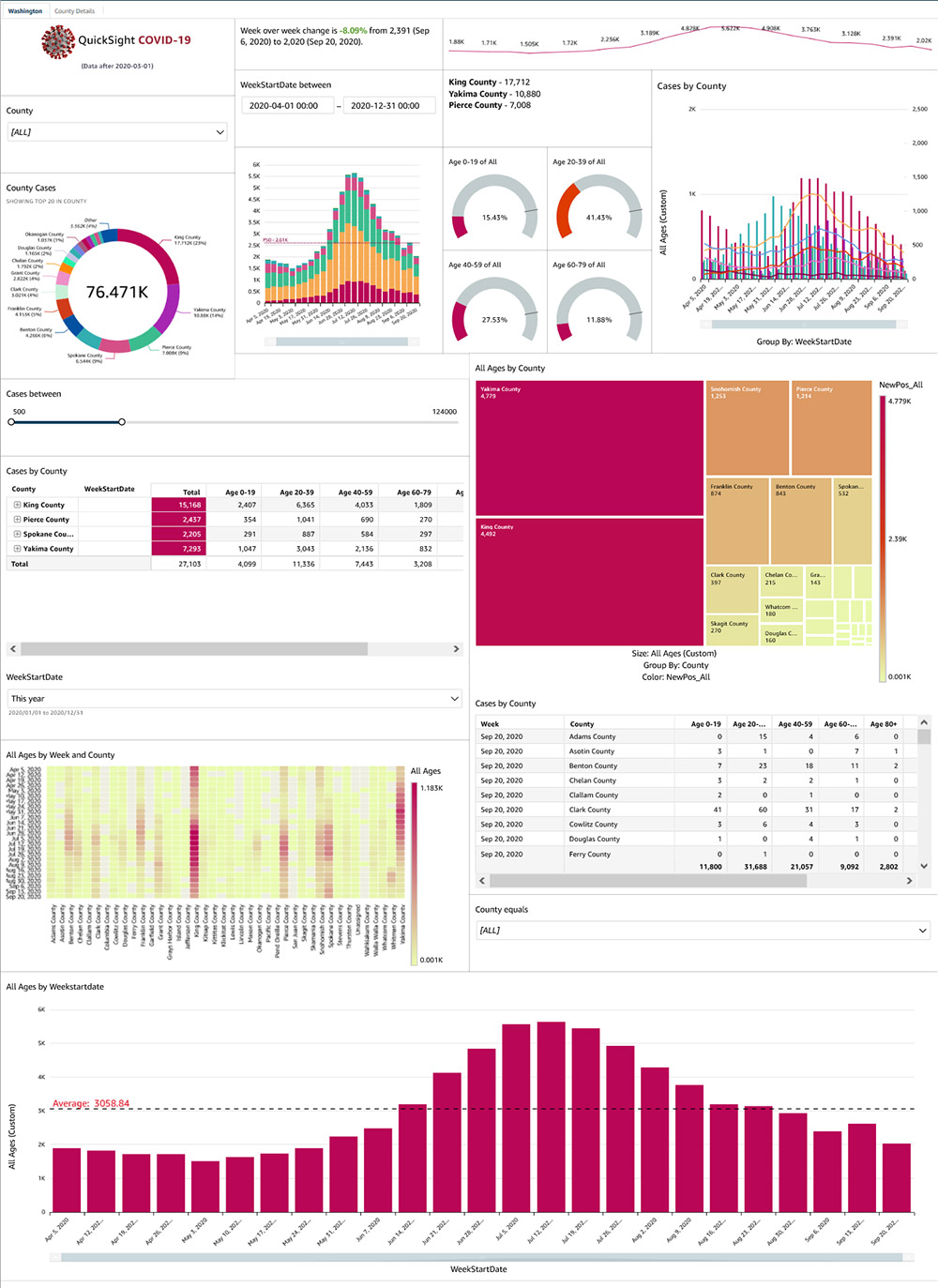
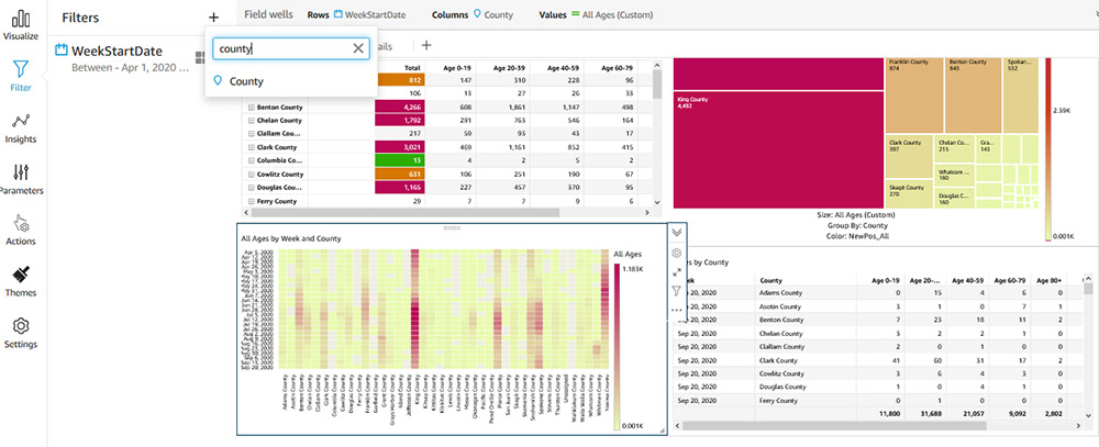
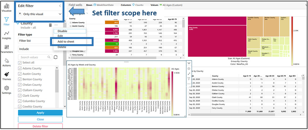
Amazon QuickSight adds support for on-sheet filter controls

Post Syndicated from Jose Kunnackal original https://aws.amazon.com/blogs/big-data/amazon-quicksight-adds-support-for-on-sheet-filter-controls/

Amazon QuickSight now supports easy and intuitive filter controls that you can place beside visuals on dashboards, allowing readers to quickly slice and dice data in the context of its visual representation. You can create these filter controls from existing or new filters with a single click, and configure them to support different operations, such as filtering specific dates, relative dates, or date rages; setting upper and lower thresholds for numeric values; adding drop-downs with single-select or multi-select options; and more.

In this post, we review how these filtering improvements, together with themes and dashboard layout options, let you create stunning, interactive dashboards that you can share with tens of thousands of users, whether in QuickSight or using embedded dashboards within apps, without any server provisioning or management needed, and paying for what you use. For this use case, we use the COVID-19 public dataset for Washington state. The following screenshot shows the dashboard with on-sheet filters added.

Using the new filter controls

Let us take a deeper look at the new filter controls, which are now placed across the sheet between visuals. Creating these controls is easy— simply add a new filter on the required dimension or metric, set the scope to either filter the entire dashboard or specific visuals within, and add it to the sheet. QuickSight now automatically maps filters across multiple datasets used within a sheet, so actions on the filter can apply to every visual on the sheet if so desired. For example, to add a new filter on the county field, create a filter on the field using the left hand navigation pane when authoring the dashboard.

Set the scope of the filter as desired, and choose Add to sheet to add a control to the sheet.

QuickSight then creates a moveable control that you can place anywhere on the sheet. QuickSight chooses the control type depending on the type of filter created. For example, when creating filters on dimensional fields, QuickSight adds a multi-select drop-down control by default. You can change the control type by choosing the Settings icon in the control’s visual menu.

In the Edit control section, you can make further updates to your control.

You can also place these controls in the control drawer on top of the sheet by choosing Pin to top.

On-sheet controls

The on-sheet controls currently supported include those previously supported with QuickSight parameter controls (single-select drop-downs, multi-select drop-downs, date and time picker, single-sided slider, single-line text box). QuickSight now supports new controls for date and time range selection, relative date selection, and numeric range selection. You can move existing parameter controls on the sheet and place them beside the new filter controls.

Let’s take a quick look at these new controls. You can use date and time range selection controls when you have a BETWEEN date range filter on your dashboard.

Relative date controls provide readers with powerful functionality to apply date filters at yearly, quarterly, monthly, weekly, daily, hourly, and minute levels. For example, you can choose to filter by current year, previous year, year to date, and last or next N years. These controls provide a great way to ensure your users always see the latest data whether viewing data in dashboards or email reports.

With a two-sided slider control, you can set lower and upper bounds on metric filters. To add a two-sided filter, you simply add the numeric BETWEEN filter to the sheet.

Additional dashboard features

In this section, we look at some other aspects of the dashboard.

Customizing your dashboard layout and theme

This dashboard uses a different set of colors and highlights than the regular palette in QuickSight. We achieve this by using a custom theme, which lets you pick a color palette for data values, background and foreground colors, fonts, and more. You can also choose to remove borders around the visual, show or remove spacing between visuals, and add margins around the sheet.

To create themes for your dashboards, go to the Themes from the left hand menu when authoring the dashboard. You can choose one of starter themes available in QuickSight and choose Save as to customize your own and use the theme editor to visualize changes before saving the theme.

On the Main page of the theme editor, you can customize your background color, foreground color, and font.

On the Data page, you can customize your data colors.

For more information about QuickSight themes, see Evolve your analytics with Amazon QuickSight’s new APIs and theming capabilities.

Images and rich text

You can use the QuickSight insight editor (available in Enterprise Edition) to add rich text and images to dashboards. To add an image, go to the insight editor, choose the Image icon, and provide the hosted location of the image. You can also hyperlink this image to any URL.

Reference lines

The bar chart within the dashboard also includes a reference line, which you can easily add to a QuickSight line or bar visual. You can configure a reference line from the visual menu.

Conditional formatting

Tables in the dashboard use conditional formatting, which you can add from the table menu.

Scaling

QuickSight dashboards default to auto-fit mode, so they are responsive based on screen size. Instead, you can choose to pick a specific screen resolution to optimize for, based on the devices your audience most commonly uses to view the dashboard. To adjust the scaling mode, choose Settings in the navigation pane while in dashboard authoring (analysis) mode.

For this post, our dashboard was built for a 1366px screen, and scales that view to a larger or smaller screen to ensure that all users see the same content (mobile devices continue to fall back to a single column, mobile-specific layout to ensure usability). Opting for the optimized mode also makes sure that your email reports look exactly like the dashboard that your viewers interact with.

Conclusion

With denser dashboards, custom themes, and new on-sheet filter controls in QuickSight, you can provide richer dashboards for your readers. Visit our user guide to learn more about on-sheet filter controls, themes, dashboard scaling options and more. For more information about authoring dashboards in QuickSight, watch Part 1 and Part 2 of our two-part interactive workshop.


About the authors

Jose Kunnackal John is a principal product manager for Amazon QuickSight.



Sahitya Pandiri is a technical program manager with Amazon Web Services. Sahitya has been in product/program management for 6 years now, and has built multiple products in the retail, healthcare, and analytics space.
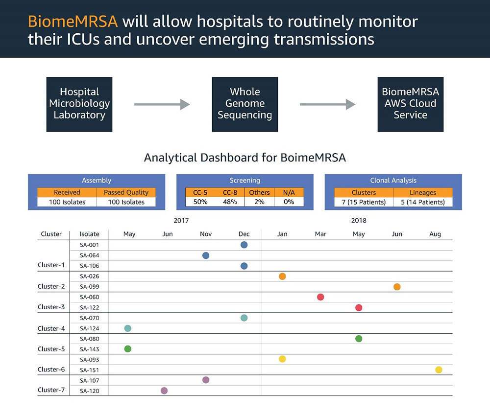
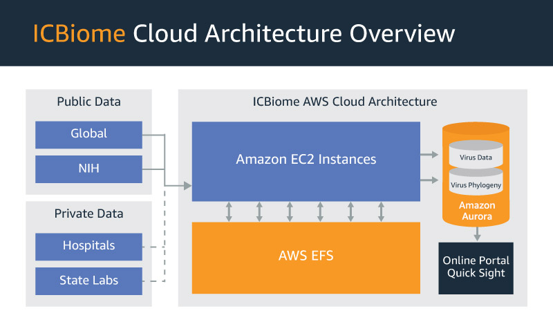



ICBiome uses Amazon QuickSight to empower hospitals in dealing with harmful pathogens

Post Syndicated from Chirag Dhull original https://aws.amazon.com/blogs/big-data/icbiome-uses-amazon-quicksight-to-empower-hospitals-in-dealing-with-harmful-pathogens/

In response to the COVID-19 pandemic, hospitals and healthcare organizations are increasingly employing genetic sequencing to screen, track, and contain harmful pathogens. ICBiome is a startup that has been working on this problem for several years, creating innovative data analytics products using AWS to help hospitals and researchers address both community-associated and hospital-acquired infections. Building on its early focus on methicillin-resistant Staphylococcus aureus (MRSA), the company is expanding its solution to cover COVID-19 and other types of infections.

ICBiome has now integrated Amazon QuickSight embedded analytics into its solution to provide hospital investigators and other users with easy access to powerful analytics and visualizations on any device.

Empowering hospitals and communities

Many hospitals lack access to sequencing capabilities, and hospitals that have such capabilities often lack complex data processing and advanced bioinformatics expertise. Open-source platforms are limited, complex, and scale poorly. They require hardware resources and management beyond the reach of most hospitals and lack visualization software to interactively explore results without specialized know-how.

BiomeMRSA, ICBiome’s cloud-based genomics service, overcomes these gaps by providing easy access to sequencing through its Clinical Laboratory Improvement Amendments (CLIA)-certified provider, with storage, computing, analytics, and visualization delivered from the AWS Cloud. With the addition of QuickSight embedded analytics, hospital investigators can easily monitor pathogens coming through their hospital environments.

Seeing the whole picture

The company’s innovative data processing methodology enables the comparison of full genomes, as opposed to open-source platforms that only compare portions of them. With a vast and growing database of MRSA mutations, the company enables rapid identification of existing and new strains to help hospitals combat infection.

BiomeMRSA monitors intensive care unit (ICU) settings and identifies emerging MRSA transmissions. By using BiomeMRSA to monitor their ICU settings, hospitals can proactively target local reservoirs and reduce overall incidence rates of MRSA. To support its R&D in pathogen genomics, the company has received more than $1 million in funding from NIAID and state grants. In 2019, ICBiome completed an evaluation of BiomeMRSA at a major hospital. It’s now evaluating and validating BiomeMRSA at two additional hospitals.

Improving patient care and treatment cost

This capability gives hospitals the potential to transform how they manage outbreaks. Intake and weekly screenings of patients lack the resolution to determine how the disease was acquired. This means hospitals can be financially and reputationally penalized for a disease that was acquired before admission.

BiomeMRSA allows continuous monitoring of ICUs by routinely sequencing all samples and returning those samples to hospitals within days. This allows for earlier detection, mitigation of outbreaks, and the reduction of colonization rates of ICU patients by identifying transmissions where the patient was colonized but not infected. Lowering colonization rates can reduce the risk of post-care infections and costly readmissions.

ICBiome is now expanding this work to include tracking pandemics such as COVID-19. The Virginia-based company is adding a COVID-19 application, BiomeCOVID, to address the ongoing crisis. Previously deployed for real-time operations, BiomeCOVID will use genetics to greatly increase the accuracy of contact tracing by separating isolates within different lineages and further identifying unique clusters within those lineages. The company is accelerating the development of BiomeCOVID to meet the critical healthcare need.

Visualizing genomics to combat disease

Since its first NIH grant award in 2017, ICBiome has built its solutions in the AWS Cloud. To deliver rich, in-depth analytics capabilities to its customers, the company chose QuickSight for embedded dashboards in its products. According to Dr. Srini Iyer, founder and CEO of ICBiome, QuickSight provides the agility and scalability the company needs to deliver in-depth solutions quickly. “ICBiome has developed an end-to-end cloud architecture for processing genetic sequence data from bacterial and viral pathogens,” says Dr. Iyer. “Over the last year, ICBiome looked at several data analytics tools that can serve as the visual interface for our product line. We did a formal analysis of both cloud and on-premises business intelligence solutions, and ultimately decided to choose QuickSight for the security, scalability, cost, and reliability.”

The following image shows the Analytics Dashboard for BiomeMRSA:

ICBiome’s customers are centered in large hospitals and public health agencies. Security and data privacy are critical to these decision-makers, particularly because bacterial and viral samples are taken from patients in the course of clinical care. QuickSight uses the same HIPAA-compliant security architecture used by the rest of the company’s data ingestion and processing systems built on AWS.

Cost-efficient and highly scalable

Scalability is critical because the company expects to handle exponentially growing amounts of data due to the growth in whole-genome sequencing to identify pathogen strains. “We opted for Amazon QuickSight as it streamlines operational scaling and integration not just within the application layer but across the entire AWS ecosystem,” says Dante Martinez, Chief Technology Officer of ICBiome.

As a startup providing affordable solutions for hospitals, cost is a critical concern for ICBiome. Many others in its space have opted to use open-source business intelligence (BI) solutions for this reason. However, the company’s analysis showed that this wasn’t the most cost-effective route. “Many open-source BI platforms require a high level of maintenance to ensure reliability both for routine operations and lifecycle management,” says Martinez. “Given the critical nature of our application, we did not want to compromise product integrity by choosing a difficult-to-maintain open-source platform or an entry-level BI tool. Amazon QuickSight is highly cost-effective, but it is also full-featured and mature, providing an experience on par with much more expensive competitors.”

The following diagram illustrates ICBiome’s cloud architecture.

Visualizing a healthier future

The company has big plans for the embedded analytics functionality enabled by QuickSight. “Once we complete the launches of BiomeCOVID and BiomeMRSA as commercial SaaS products, we intend to bring to market other surveillance products such as BiomeCRE and BiomeSTD to track other critical threats to public health,” says Dr. Iyer. “We will also be targeting other biomedical areas where we can develop new classes of products that provide critical data analytical capabilities that are currently not feasible.”

With the landscape of public health now transformed in the wake of the COVID-19 pandemic, ICBiome will continue to expand its SaaS portfolio with Amazon to provide hospitals innovative data analytics tools in infection prevention, epidemiology, and patient care.


About the  Author

Chirag Dhull is a Principal Product Marketing Manager for Amazon QuickSight.
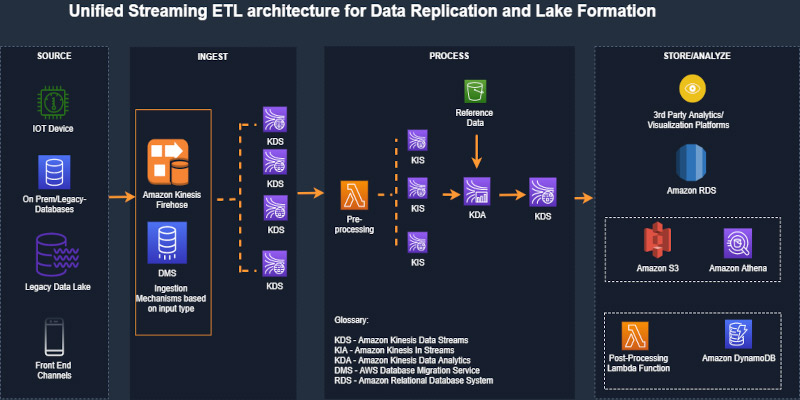
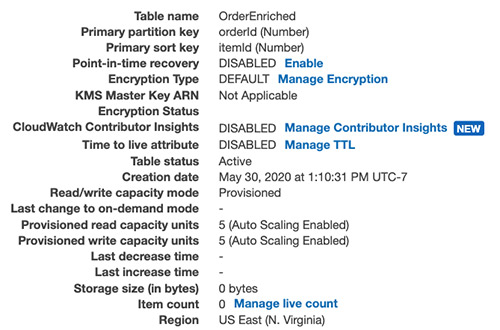


Unified serverless streaming ETL architecture with Amazon Kinesis Data Analytics

Post Syndicated from Ram Vittal original https://aws.amazon.com/blogs/big-data/unified-serverless-streaming-etl-architecture-with-amazon-kinesis-data-analytics/

Businesses across the world are seeing a massive influx of data at an enormous pace through multiple channels. With the advent of cloud computing, many companies are realizing the benefits of getting their data into the cloud to gain meaningful insights and save costs on data processing and storage. As businesses embark on their journey towards cloud solutions, they often come across challenges involving building serverless, streaming, real-time ETL (extract, transform, load) architecture that enables them to extract events from multiple streaming sources, correlate those streaming events, perform enrichments, run streaming analytics, and build data lakes from streaming events.

In this post, we discuss the concept of unified streaming ETL architecture using a generic serverless streaming architecture with Amazon Kinesis Data Analytics at the heart of the architecture for event correlation and enrichments. This solution can address a variety of streaming use cases with various input sources and output destinations. We then walk through a specific implementation of the generic serverless unified streaming architecture that you can deploy into your own AWS account for experimenting and evolving this architecture to address your business challenges.

Overview of solution

As data sources grow in volume, variety, and velocity, the management of data and event correlation become more challenging. Most of the challenges stem from data silos, in which different teams and applications manage data and events using their own tools and processes.

Modern businesses need a single, unified view of the data environment to get meaningful insights through streaming multi-joins, such as the correlation of sensory events and time-series data. Event correlation plays a vital role in automatically reducing noise and allowing the team to focus on those issues that really matter to the business objectives.

To realize this outcome, the solution proposes creating a three-stage architecture:

  • Ingestion
  • Processing
  • Analysis and visualization

The source can be a varied set of inputs comprising structured datasets like databases or raw data feeds like sensor data that can be ingested as single or multiple parallel streams. The solution envisions multiple hybrid data sources as well. After it’s ingested, the data is divided into single or multiple data streams depending on the use case and passed through a preprocessor (via an AWS Lambda function). This highly customizable processor transforms and cleanses data to be processed through analytics application. Furthermore, the architecture allows you to enrich data or validate it against standard sets of reference data, for example validating against postal codes for address data received from the source to verify its accuracy. After the data is processed, it’s sent to various sink platforms depending on your preferences, which could range from storage solutions to visualization solutions, or even stored as a dataset in a high-performance database.

The solution is designed with flexibility as a key tenant to address multiple, real-world use cases. The following diagram illustrates the solution architecture.

The architecture has the following workflow:

  1. We use AWS Database Migration Service (AWS DMS) to push records from the data source into AWS in real time or batch. For our use case, we use AWS DMS to fetch records from an on-premises relational database.
  2. AWS DMS writes records to Amazon Kinesis Data Streams. The data is split into multiple streams as necessitated through the channels.
  3. A Lambda function picks up the data stream records and preprocesses them (adding the record type). This is an optional step, depending on your use case.
  4. Processed records are sent to the Kinesis Data Analytics application for querying and correlating in-application streams, taking into account Amazon Simple Storage Service (Amazon S3) reference data for enrichment.

Solution walkthrough

For this post, we demonstrate an implementation of the unified streaming ETL architecture using Amazon RDS for MySQL as the data source and Amazon DynamoDB as the target. We use a simple order service data model that comprises orders, items, and products, where an order can have multiple items and the product is linked to an item in a reference relationship that provides detail about the item, such as description and price.

We implement a streaming serverless data pipeline that ingests orders and items as they are recorded in the source system into Kinesis Data Streams via AWS DMS. We build a Kinesis Data Analytics application that correlates orders and items along with reference product information and creates a unified and enriched record. Kinesis Data Analytics outputs output this unified and enriched data to Kinesis Data Streams. A Lambda function consumer processes the data stream and writes the unified and enriched data to DynamoDB.

To launch this solution in your AWS account, use the GitHub repo.

Prerequisites

Before you get started, make sure you have the following prerequisites:

Setting up AWS resources in your account

To set up your resources for this walkthrough, complete the following steps:

  1. Set up the AWS CDK for Java on your local workstation. For instructions, see Getting Started with the AWS CDK.
  2. Install Maven binaries for Java if you don’t have Maven installed already.
  3. If this is the first installation of the AWS CDK, make sure to run cdk bootstrap.
  4. Clone the following GitHub repo.
  5. Navigate to the project root folder and run the following commands to build and deploy:
    1. mvn compile
    2. cdk deploy UnifiedStreamETLCommonStack UnifiedStreamETLDataStack UnifiedStreamETLProcessStack

Setting up the orders data model for CDC

In this next step, you set up the orders data model for change data capture (CDC).

  1. On the Amazon Relational Database Service (Amazon RDS) console, choose Databases.
  2. Choose your database and make sure that you can connect to it securely for testing using bastion host or other mechanisms (not detailed in scope of this post).
  3. Start MySQL Workbench and connect to your database using your DB endpoint and credentials.
  4. To create the data model in your Amazon RDS for MySQL database, run orderdb-setup.sql.
  5. On the AWS DMS console, test the connections to your source and target endpoints.
  6. Choose Database migration tasks.
  7. Choose your AWS DMS task and choose Table statistics.
  8. To update your table statistics, restart the migration task (with full load) for replication.
  9. From your MySQL Workbench session, run orders-data-setup.sql to create orders and items.
  10. Verify that CDC is working by checking the Table statistics

Setting up your Kinesis Data Analytics application

To set up your Kinesis Data Analytics application, complete the following steps:

  1. Upload the product reference products.json to your S3 bucket with the logical ID prefix unifiedBucketId (which was previously created by cdk deploy).

You can now create a Kinesis Data Analytics application and map the resources to the data fields.

  1. On the Amazon Kinesis console, choose Analytics Application.
  2. Choose Create application.
  3. For Runtime, choose SQL.
  4. Connect the streaming data created using the AWS CDK as a unified order stream.
  5. Choose Discover schema and wait for it to discover the schema for the unified order stream. If discovery fails, update the records on the source Amazon RDS tables and send streaming CDC records.
  6. Save and move to the next step.
  7. Connect the reference S3 bucket you created with the AWS CDK and uploaded with the reference data.
  8. Input the following:
    1. “products.json” on the path to the S3 object
    2. Products on the in-application reference table name
  9. Discover the schema, then save and close.
  10. Choose SQL Editor and start the Kinesis Data Analytics application.
  11. Edit the schema for SOURCE_SQL_STREAM_001 and map the data resources as follows:
Column Name Column Type Row Path
orderId INTEGER $.data.orderId
itemId INTEGER $.data.orderId
itemQuantity INTEGER $.data.itemQuantity
itemAmount REAL $.data.itemAmount
itemStatus VARCHAR $.data.itemStatus
COL_timestamp VARCHAR $.metadata.timestamp
recordType VARCHAR $.metadata.table-name
operation VARCHAR $.metadata.operation
partitionkeytype VARCHAR $.metadata.partition-key-type
schemaname VARCHAR $.metadata.schema-name
tablename VARCHAR $.metadata.table-name
transactionid BIGINT $.metadata.transaction-id
orderAmount DOUBLE $.data.orderAmount
orderStatus VARCHAR $.data.orderStatus
orderDateTime TIMESTAMP $.data.orderDateTime
shipToName VARCHAR $.data.shipToName
shipToAddress VARCHAR $.data.shipToAddress
shipToCity VARCHAR $.data.shipToCity
shipToState VARCHAR $.data.shipToState
shipToZip VARCHAR $.data.shipToZip


  1. Choose Save schema and update stream samples.

When it’s complete, verify for 1 minute that nothing is in the error stream. If an error occurs, check that you defined the schema correctly.

  1. On your Kinesis Data Analytics application, choose your application and choose Real-time analytics.
  2. Go to the SQL results and run kda-orders-setup.sql to create in-application streams.
  3. From the application, choose Connect to destination.
  4. For Kinesis data stream, choose unifiedOrderEnrichedStream.
  5. For In-application stream, choose ORDER_ITEM_ENRICHED_STREAM.
  6. Choose Save and Continue.

Testing the unified streaming ETL architecture

You’re now ready to test your architecture.

  1. Navigate to your Kinesis Data Analytics application.
  2. Choose your app and choose Real-time analytics.
  3. Go to the SQL results and choose Real-time analytics.
  4. Choose the in-application stream ORDER_ITEM_ENRCIHED_STREAM to see the results of the real-time join of records from the order and order item streaming Kinesis events.
  5. On the Lambda console, search for UnifiedStreamETLProcess.
  6. Choose the function and choose Monitoring, Recent invocations.
  7. Verify the Lambda function run results.
  8. On the DynamoDB console, choose the OrderEnriched table.
  9. Verify the unified and enriched records that combine order, item, and product records.

The following screenshot shows the OrderEnriched table.

Operational aspects

When you’re ready to operationalize this architecture for your workloads, you need to consider several aspects:

  • Monitoring metrics for Kinesis Data Streams: GetRecords.IteratorAgeMilliseconds, ReadProvisionedThroughputExceeded, and WriteProvisionedThroughputExceeded
  • Monitoring metrics available for the Lambda function, including but not limited to Duration, IteratorAge, Error count and success rate (%), Concurrent executions, and Throttles
  • Monitoring metrics for Kinesis Data Analytics (millisBehindLatest)
  • Monitoring DynamoDB provisioned read and write capacity units
  • Using the DynamoDB automatic scaling feature to automatically manage throughput

We used the solution architecture with the following configuration settings to evaluate the operational performance:

  • Kinesis OrdersStream with two shards and Kinesis OrdersEnrichedStream with two shards
  • The Lambda function code does asynchronous processing with Kinesis OrdersEnrichedStream records in concurrent batches of five, with batch size as 500
  • DynamoDB provisioned WCU is 3000, RCU is 300

We observed the following results:

  • 100,000 order items are enriched with order event data and product reference data and persisted to DynamoDB
  • An average of 900 milliseconds latency from the time of event ingestion to the Kinesis pipeline to when the record landed in DynamoDB

The following screenshot shows the visualizations of these metrics.

Cleaning up

To avoid incurring future charges, delete the resources you created as part of this post (the AWS CDK provisioned AWS CloudFormation stacks).

Conclusion

In this post, we designed a unified streaming architecture that extracts events from multiple streaming sources, correlates and performs enrichments on events, and persists those events to destinations. We then reviewed a use case and walked through the code for ingesting, correlating, and consuming real-time streaming data with Amazon Kinesis, using Amazon RDS for MySQL as the source and DynamoDB as the target.

Managing an ETL pipeline through Kinesis Data Analytics provides a cost-effective unified solution to real-time and batch database migrations using common technical knowledge skills like SQL querying.


About the Authors

Ram Vittal is an enterprise solutions architect at AWS. His current focus is to help enterprise customers with their cloud adoption and optimization journey to improve their business outcomes. In his spare time, he enjoys tennis, photography, and movies.


Akash Bhatia is a Sr. solutions architect at AWS. His current focus is helping customers achieve their business outcomes through architecting and implementing innovative and resilient solutions at scale.


Normalize data with Amazon Elasticsearch Service ingest pipelines

Post Syndicated from Vijay Injam original https://aws.amazon.com/blogs/big-data/normalize-data-with-amazon-elasticsearch-service-ingest-pipelines/

Amazon Elasticsearch Service (Amazon ES) is a fully managed service that makes it easy for you to deploy, secure, and run Elasticsearch cost-effectively at scale. Search and log analytics are the two most popular use cases for Amazon ES. In log analytics at scale, a common pattern is to create indexes from multiple sources. In these use cases, how can you ensure that all the incoming data follows a specific, predefined format if it’s operationally not feasible to apply checks in each data source? You can use Elasticsearch ingest pipelines to normalize all the incoming data and create indexes with the predefined format.

What’s an ingest pipeline?

An ingest pipeline lets you use some of your Amazon ES domain processing power to apply to a set of processors during indexing. Ingest pipeline applies processors in order, the output of one processor moving to the next processor in the pipe. You define a pipeline with the Elasticsearch _ingest API. The following screenshot illustrates this architecture.

To find the available ingest processors in your Amazon ES domain, enter the following code:

GET _ingest/pipeline/

Solution overview

In this post, we discuss three log analytics use cases where data normalization is a common technique.

We create three pipelines and normalize the data for each use case. The following diagram illustrates this architecture.

Use case 1

In this first use case, Amazon ES domain has three sources: logstash, Fluentd, and AWS Lambda. Your logstash source sends the data to an index with the name index-YYYY.MM.DD.HH (hours in the end). When you have an error in the Fluentd source, it creates the index named index-YYYY.MM.DD (missing the hours). Your domain creates indexes for both the formats, which is not what you intended.

One way to correct the index name is to calculate the hours of the ingested data and assign the value to the index. If you can’t identify any pattern, or identify further issues to the indexing name, you need to segregate the data to a different index (for example, format_error) for further analysis.

Use case 2

If your application uses time-series data and analyzes data from fixed time windows, your data sources can sometimes send data from a prior time window. In this use case, you need to check for the incoming data and discard data that doesn’t fit in the current time window.

Use case 3

In some use cases, the value for a key can contain large strings with common prefixes. End-users typically use wild card characters (*) with the prefix to search on these fields. If your application or Kibana dashboards contain several wild card queries, it can increase CPU utilization and overall search lateness. You can address this by identifying the prefixes from the values and creating a new field with the data type as a keyword. You can use Term queries for the keywords and improve search performance.

Pipeline 1: pipeline_normalize_index

The default pipeline for incoming data is pipeline_normalize_index. This pipeline performs the following actions:

  • Checks if the incoming data belongs to the current date.
  • Checks if the data has any errors in the index name.
  • Segregates the data:
    • If it doesn’t find any errors, it pushes the data to pipeline_normalize_data.
    • If it finds errors, it pushes the pipeline to pipeline_fix_index.

Checking the index date

In this step, you can create an index pipeline using a script processor, which lets you create a script and execute within the pipeline.

Use the Set processor to add _ingest.timestamp to doc_received_date and compare the index date to the document received date. The script processor lets you create a script using painless scripts. You can create a script to check if the index date matches the doc_received_date. The script processor let you access the ingest document using the ctx variable. See the following code:

       "set":{
            "field":"doc_received_date",
            "value":"{{_ingest.timestamp}}"
         }
      },
      {
         "script":{
            "lang":"painless",
            "source": """
                    DateTimeFormatter formatter = DateTimeFormatter.ofPattern("yyyy.MM.dd");
                    String dateandhour = ctx._index.substring(ctx._index.indexOf('-') + 1);
                    LocalDate indexdate = LocalDate.parse(dateandhour.substring(0, 10), formatter);
                    ZonedDateTime zonedDateTime = ZonedDateTime.parse(ctx.doc_received_date, DateTimeFormatter.ISO_DATE_TIME);
                    LocalDate doc_received_date = zonedDateTime.toLocalDate();
                    if (doc_received_date.isEqual(indexdate)) {
                        ctx.index_purge = "N";
                    } else {
                        ctx.index_purge = "Y";
                    }
                    if (dateandhour.length() > 10) {
                        ctx.indexformat_error = "N";
                    } else {
                        ctx.indexformat_error = "Y";
                    }
        """,

Checking for index name errors

You can use the same script processor from the previous step to check if the index name matches the format index-YYYY.MM.DD.HH or index-YYYY.MM.DD. See the following code:

if (dateandhour.length() > 10) {
                        ctx.indexformat_error = "N";
                    } else {
                        ctx.indexformat_error = "Y";
                    }

Segregating the data

If the index date doesn’t match the _ingest.timestamp, you can drop the request using the drop processor. If the index name doesn’t match the format index-YYYY.MM.DD, you can segregate the data to pipeline pipeline_verify_index_date and proceed to the pipeline pipeline_normalize_data. If conditions aren’t met, you can proceed to the pipeline pipeline_indexformat_errors or assign a default index indexing_errors. If no are issues found, you proceed to the pipeline pipeline_normalize_data. See the following code:

 "pipeline":{
            "if":"ctx.indexformat_error == 'Y'",
            "name":"pipeline_fix_index_name"
         }
      },
      {
         "remove":{
            "field":[
               "doc_received_date",
               "index_purge",
               "indexformat_error"
            ],
            "ignore_missing":true
         }
      },
      {
         "pipeline":{
            "name":"pipeline_normalize_data"

The following code is an example pipeline:

PUT _ingest/pipeline/pipeline_normalize_index
{
   "description":"pipeline_normalize_index",
   "processors":[
      {
         "set":{
            "field":"doc_received_date",
            "value":"{{_ingest.timestamp}}"
         }
      },
      {
         "script":{
            "lang":"painless",
            "source": """
                    DateTimeFormatter formatter = DateTimeFormatter.ofPattern("yyyy.MM.dd");
                    String dateandhour = ctx._index.substring(ctx._index.indexOf('-') + 1);
                    LocalDate indexdate = LocalDate.parse(dateandhour.substring(0, 10), formatter);
                    ZonedDateTime zonedDateTime = ZonedDateTime.parse(ctx.doc_received_date, DateTimeFormatter.ISO_DATE_TIME);
                    LocalDate doc_received_date = zonedDateTime.toLocalDate();
                    if (doc_received_date.isEqual(indexdate)) {
                        ctx.index_purge = "N";
                    } else {
                        ctx.index_purge = "Y";
                    }
                    if (dateandhour.length() > 10) {
                        ctx.indexformat_error = "N";
                    } else {
                        ctx.indexformat_error = "Y";
                    }
        """,
         "on_failure":[
            {
               "set":{
                  "field":"Amazon_es_PipelineError",
                  "value":"at Script processor - Purge older Index or Index date error"
               }
            },
            {
               "set":{
                  "field":"_index",
                  "value":"indexing_errors"
               }
            }
         ]
      },
      {
         "drop":{
            "if":"ctx.index_purge == 'Y'"
         }
      },
      {
         "pipeline":{
            "if":"ctx.indexformat_error == 'Y'",
            "name":"pipeline_fix_index_name"
         }
      },
      {
         "remove":{
            "field":[
               "doc_received_date",
               "index_purge",
               "indexformat_error"
            ],
            "ignore_missing":true
         }
      },
      {
         "pipeline":{
            "name":"pipeline_normalize_data"
         }
      }
   ]
}

Pipeline 2: pipeline_normalize_data

The pipeline pipeline_normalize_data fixes index data. It extracts the prefix from the defined field and creates a new field. You can use the new field for Term queries.

In this step, you can use a grok processor to extract prefixes from the existing fields and create a new field that you can use for term queries. The output of this pipeline creates the index. See the following code of an example pipeline:

PUT _ingest/pipeline/pipeline_normalize_data
{
  "description":"pipeline_normalize_data",
  "version":1,
  "processors":[
     {
        "grok":{
           "field":"application_type",
           "patterns":[
              "%{WORD:application_group}"
           ],
           "ignore_missing":true,
           "on_failure":[
              {
                 "set":{
                    "field":"Amazon_es_PipelineError",
                    "value":"application_type error"
                 }
              }
           ]
        }
     }
  ]
}

Pipeline 3: pipeline_fix_index

This pipeline fixes the index name. The indexing errors identified in pipeline_normalize_Index are the incoming data points for this pipeline. pipeline_fix_index extracts the hours from the _ingest.timestamp and appends it to the index name.

The index name errors identified from Pipeline 1 are the data source for this pipeline. You can use the script processor to write a painless script. The script extracts hours (HH) from the _ingest.timestamp and appends it to the _index. See the following code of the example pipeline:

PUT _ingest/pipeline/pipeline_fix_index_name
    {
      "description":"pipeline_fix_index_name",
      "processors":[
         {
            "set":{
               "field":"doc_received_date",
               "value":"{{_ingest.timestamp}}"
            }
         },
         {
            "script":{
               "lang":"painless",
               "source": 
               """
               ZonedDateTime zonedDateTime = ZonedDateTime.parse(ctx.doc_received_date, DateTimeFormatter.ISO_DATE_TIME);
               LocalDate doc_received_date = zonedDateTime.toLocalDate();
               String receiveddatehour = zonedDateTime.getHour().toString();
               if (zonedDateTime.getHour() < 10) {
                    receiveddatehour = "0" + zonedDateTime.getHour();
               }
               ctx._index = ctx._index + "." + receiveddatehour;
               """,
               "on_failure":[
                  {
                     "set":{
                        "field":"Amazon_es_PipelineError",
                        "value":"at Script processor - Purge older Index or Index date error"
                     }
                  },
                  {
                     "set":{
                        "field":"_index",
                        "value":"indexformat_errors"
                     }
                  }
               ]
            }
         },
         {
            "remove":{
               "field":[
                  "doc_received_date"
               ],
               "ignore_missing":true
            }
         },
         {
            "pipeline":{
               "name":"pipeline_normalize_data"
            }
         }
      ]
   }

Adding the default pipeline to the index template

After creating all the pipelines, add the default pipeline to the index template. See the following code:

"default_pipeline" : "pipeline_normalize_index"

Summary

You can normalize data, fix indexing errors, and segregate operation data and anomalies by using ingest pipelines. Although you can use one pipeline with several processors (depending on the use case), indexing pipelines provides an efficient way to utilize compute resources and operational resources by eliminating unwanted indexes.


About the Author

Vijay Injam is a Data Architect with Amazon Web Services.



Kevin Fallis is an AWS specialist search solutions architect. His passion at AWS is to help customers leverage the correct mix of AWS services to achieve success for their business goals. His after-work activities include family, DIY projects, carpentry, playing drums, and all things music.

Free, Privacy-First Analytics for a Better Web

Post Syndicated from Jon Levine original https://blog.cloudflare.com/free-privacy-first-analytics-for-a-better-web/

Free, Privacy-First Analytics for a Better Web

Everyone with a website needs to know some basic facts about their website: what pages are people visiting? Where in the world are they? What other sites sent traffic to my website?

There are “free” analytics tools out there, but they come at a cost: not money, but your users’ privacy. Today we’re announcing a brand new, privacy-first analytics service that’s open to everyone — even if they’re not already a Cloudflare customer. And if you’re a Cloudflare customer, we’ve enhanced our analytics to make them even more powerful than before.

The most important analytics feature: Privacy

The most popular analytics services available were built to help ad-supported sites sell more ads. But, a lot of websites don’t have ads. So if you use those services, you’re giving up the privacy of your users in order to understand how what you’ve put online is performing.

Cloudflare’s business has never been built around tracking users or selling advertising. We don’t want to know what you do on the Internet — it’s not our business. So we wanted to build an analytics service that gets back to what really matters for web creators, not necessarily marketers, and to give web creators the information they need in a simple, clean way that doesn’t sacrifice their visitors’ privacy. And giving web creators these analytics shouldn’t depend on their use of Cloudflare’s infrastructure for performance and security. (More on that in a bit.)

What does it mean for us to make our analytics “privacy-first”? Most importantly, it means we don’t need to track individual users over time for the purposes of serving analytics. We don’t use any client-side state, like cookies or localStorage, for the purposes of tracking users. And we don’t “fingerprint” individuals via their IP address, User Agent string, or any other data for the purpose of displaying analytics. (We consider fingerprinting even more intrusive than cookies, because users have no way to opt out.)

Counting visits without tracking users

One of the most essential stats about any website is: “how many people went there”? Analytics tools frequently show counts of “unique” visitors, which requires tracking individual users by a cookie or IP address.

We use the concept of a visit: a privacy-friendly measure of how people have interacted with your website. A visit is defined simply as a successful page view that has an HTTP referer that doesn’t match the hostname of the request. This tells you how many times people came to your website and clicked around before navigating away, but doesn’t require tracking individuals.

Free, Privacy-First Analytics for a Better Web

A visit has slightly different semantics from a “unique”, and you should expect this number to differ from other analytics tools.

All of the details, none of the bots

Our analytics deliver the most important metrics about your website, like page views and visits. But we know that an essential analytics feature is flexibility: the ability to add arbitrary filters, and slice-and-dice data as you see fit. Our analytics can show you the top hostnames, URLs, countries, and other critical metrics like status codes. You can filter on any of these metrics with a click and see the whole dashboard update.

I’m especially excited about two features in our time series charts: the ability to drag-to-zoom into a narrower time range, and the ability to “group by” different dimensions to see data in a different way. This is a super powerful way to drill into an anomaly in traffic and quickly see what’s going on. For example, you might notice a spike in traffic, zoom into that spike, and then try different groupings to see what contributed the extra clicks. A GIF is worth a thousand words:

And for customers of our Bot Management product, we’re working on the ability to detect (and remove) automated traffic. Coming very soon, you’ll be able to see which bots are reaching your website — with just a click, block them by using Firewall Rules.

This is all possible thanks to our ABR analytics technology, which enables us to serve analytics very quickly for websites large and small. Check out our blog post to learn more about how this works.

Edge or Browser analytics? Why not both?

There are two ways to collect web analytics data: at the edge (or on an origin server), or in the client using a JavaScript beacon.

Historically, Cloudflare has collected analytics data at our edge. This has some nice benefits over traditional, client-side analytics approaches:

  • It’s more accurate because you don’t miss users who block third-party scripts, or JavaScript altogether
  • You can see all of the traffic back to your origin server, even if an HTML page doesn’t load
  • We can detect (and block bots), apply Firewall rules, and generally scrub traffic of unwanted noise
  • You can measure the performance of your origin server

More commonly, most web analytics providers use client-side measurement. This has some benefits as well:

  • You can understand performance as your users see it — e.g. how long did the page actually take to render
  • You can detect errors in client-side JavaScript execution
  • You can define custom event types emitted by JavaScript frameworks

Ultimately, we want our customers to have the best of both worlds. We think it’s really powerful to get web traffic numbers directly from the edge. We also launched Browser Insights a year ago to augment our existing edge analytics with more performance information, and today Browser Insights are taking a big step forward by incorporating Web Vitals metrics.

But, we know not everyone can modify their DNS to take advantage of Cloudflare’s edge services. That’s why today we’re announcing a free, standalone analytics product for everyone.

How do I get it?

For existing Cloudflare customers on our Pro, Biz, and Enterprise plans, just go to your Analytics tab! Starting today, you’ll see a banner to opt-in to the new analytics experience. (We plan to make this the default in a few weeks.)

But when building privacy-first analytics, we realized it’s important to make this accessible even to folks who don’t use Cloudflare today. You’ll be able to use Cloudflare’s web analytics even if you can’t change your DNS servers — just add our JavaScript, and you’re good to go.

We’re still putting on the finishing touches on our JavaScript-based analytics, but you can sign up here and we’ll let you know when it’s ready.

The evolution of analytics at Cloudflare

Just over a year ago, Cloudflare’s analytics consisted of a simple set of metrics: cached vs uncached data transfer, or how many requests were blocked by the Firewall. Today we provide flexible, powerful analytics across all our products, including Firewall, Cache, Load Balancing and Network traffic.

While we’ve been focused on building analytics about our products, we realized that our analytics are also powerful as a standalone product. Today is just the first step on that journey. We have so much more planned: from real-time analytics, to ever-more performance analysis, and even allowing customers to add custom events.

We want to hear what you want most out of analytics — drop a note in the comments to let us know what you want to see next.

Explaining Cloudflare’s ABR Analytics

Post Syndicated from Jamie Herre original https://blog.cloudflare.com/explaining-cloudflares-abr-analytics/

Explaining Cloudflare's ABR Analytics

Cloudflare’s analytics products help customers answer questions about their traffic by analyzing the mind-boggling, ever-increasing number of events (HTTP requests, Workers requests, Spectrum events) logged by Cloudflare products every day.  The answers to these questions depend on the point of view of the question being asked, and we’ve come up with a way to exploit this fact to improve the quality and responsiveness of our analytics.

Useful Accuracy

Consider the following questions and answers:

What is the length of the coastline of Great Britain? 12.4K km
What is the total world population? 7.8B
How many stars are in the Milky Way? 250B
What is the total volume of the Antarctic ice shelf? 25.4M km3
What is the worldwide production of lentils? 6.3M tonnes
How many HTTP requests hit my site in the last week? 22.6M

Useful answers do not benefit from being overly exact.  For large quantities, knowing the correct order of magnitude and a few significant digits gives the most useful answer.  At Cloudflare, the difference in traffic between different sites or when a single site is under attack can cross nine orders of magnitude and, in general, all our traffic follows a Pareto distribution, meaning that what’s appropriate for one site or one moment in time might not work for another.

Explaining Cloudflare's ABR Analytics

Because of this distribution, a query that scans a few hundred records for one customer will need to scan billions for another.  A report that needs to load a handful of rows under normal operation might need to load millions when a site is under attack.

To get a sense of the relative difference of each of these numbers, remember “Powers of Ten”, an amazing visualization that Ray and Charles Eames produced in 1977.  Notice that the scale of an image determines what resolution is practical for recording and displaying it.

Explaining Cloudflare's ABR Analytics

Using ABR to determine resolution

This basic fact informed our design and implementation of ABR for Cloudflare analytics.  ABR stands for “Adaptive Bit Rate”.  It’s essentially an eponym for the term as used in video streaming such as Cloudflare’s own Stream Delivery.  In those cases, the server will select the best resolution for a video stream to match your client and network connection.

In our case, every analytics query that supports ABR will be calculated at a resolution matching the query.  For example, if you’re interested to know from which country the most firewall events were generated in the past week, the system might opt to use a lower resolution version of the firewall data than if you had opted to look at the last hour. The lower resolution version will provide the same answer but take less time and fewer resources.  By using multiple, different resolutions of the same data, our analytics can provide consistent response times and a better user experience.

You might be aware that we use a columnar store called ClickHouse to store and process our analytics data.  When using ABR with ClickHouse, we write the same data at multiple resolutions into separate tables.  Usually, we cover seven orders of magnitude – from 100% to 0.0001% of the original events.  We wind up using an additional 12% of disk storage but enable very fast ad hoc queries on the reduced resolution tables.

Explaining Cloudflare's ABR Analytics

Aggregations and Rollups

The ABR technique facilitates aggregations by making compact estimates of every dimension.  Another way to achieve the same ends is with a system that computes “rollups”.  Rollups save space by computing either complete or partial aggregations of the data as it arrives.  

For example, suppose we wanted to count a total number of lentils. (Lentils are legumes and among the oldest and most widely cultivated crops.  They are a staple food in many parts of the world.)  We could just count each lentil as it passed through the processing system. Of course because there a lot of lentils, that system is distributed – meaning that there are hundreds of separate machines.  Therefore we’ll actually have hundreds of separate counters.

Also, we’ll want to include more information than just the count, so we’ll also include the weight of each lentil and maybe 10 or 20 other attributes. And of course, we don’t want just a total for each attribute, but we’ll want to be able to break it down by color, origin, distributor and many other things, and also we’ll want to break these down by slices of time.

In the end, we’ll have tens of thousands or possibly millions of aggregations to be tabulated and saved every minute.  These aggregations are expensive to compute, especially when using aggregations more complicated than simple counters and sums.  They also destroy some information.  For example, once we’ve processed all the lentils through the rollups, we can’t say for sure that we’ve counted them all, and most importantly, whichever attributes we neglected to aggregate are unavailable.

The number we’re counting, 6.3M tonnes, only includes two significant digits which can easily be achieved by counting a sample.  Most of the rollup computations used on each lentil (on the order 1013 to account for 6.3M tonnes) are wasted.

Other forms of aggregations

So far, we’ve discussed ABR and its application to aggregations, but we’ve only given examples involving “counts” and “sums”.  There are other, more complex forms of aggregations we use quite heavily.  Two examples are “topK” and “count-distinct”.

A “topK” aggregation attempts to show the K most frequent items in a set.  For example, the most frequent IP address, or country.  To compute topK, just count the frequency of each item in the set and return the K items with the highest frequencies. Under ABR, we compute topK based on the set found in the matching resolution sample. Using a sample makes this computation a lot faster and less complex, but there are problems.

The estimate of topK derived from a sample is biased and dependent on the distribution of the underlying data. This can result in overestimating the significance of elements in the set as compared to their frequency in the full set. In practice this effect can only be noticed when the cardinality of the set is very high and you’re not going to notice this effect on a Cloudflare dashboard.  If your site has a lot of traffic and you’re looking at the Top K URLs or browser types, there will be no difference visible at different resolutions.  Also keep in mind that as long as we’re estimating the “proportion” of the element in the set and the set is large, the results will be quite accurate.

The other fascinating aggregation we support is known as “count-distinct”, or number of uniques.  In this case we want to know the number of unique values in a set.  For example, how many unique cache keys have been used.  We can safely say that a uniform random sample of the set cannot be used to estimate this number.  However, we do have a solution.

We can generate another, alternate sample based on the value in question.  For example, instead of taking a random sample of all requests, we take a random sample of IP addresses.  This is sometimes called distinct reservoir sampling, and it allows us to estimate the true number of distinct IPs based on the cardinality of the sampled set. Again, there are techniques available to improve these estimates, and we’ll be implementing some of those.

ABR improves resilience and scalability

Using ABR saves us resources.  Even better, it allows us to query all the attributes in the original data, not just those included in rollups.  And even better, it allows us to check our assumptions against different sample intervals in separate tables as a check that the system is working correctly, because the original events are preserved.

However, the greatest benefits of employing ABR are the ones that aren’t directly visible. Even under ideal conditions, a large distributed system such as Cloudflare’s data pipeline is subject to high tail latency.  This occurs when any single part of the system takes longer than usual for any number of a long list of reasons.  In these cases, the ABR system will adapt to provide the best results available at that moment in time.

For example, compare this chart showing Cache Performance for a site under attack with the same chart generated a moment later while we simulate a failure of some of the servers in our cluster.  In the days before ABR, your Cloudflare dashboard would fail to load in this scenario.  Now, with ABR analytics, you won’t see significant degradation.

Explaining Cloudflare's ABR Analytics

Stretching the analogy to ABR in video streaming, we want you to be able to enjoy your analytics dashboard without being bothered by issues related to faulty servers, or network latency, or long running queries.  With ABR you can get appropriate answers to your questions reliably and within a predictable amount of time.

In the coming months, we’re going to be releasing a variety of new dashboards and analytics products based on this simple but profound technology.  Watch your Cloudflare dashboard for increasingly useful and interactive analytics.

Start measuring Web Vitals with Browser Insights

Post Syndicated from Jon Levine original https://blog.cloudflare.com/start-measuring-web-vitals-with-browser-insights/

Start measuring Web Vitals with Browser Insights

Many of us at Cloudflare obsess about how to make websites faster. But to improve performance, you have to measure it first. Last year we launched Browser Insights to help our customers measure web performance from the perspective of end users.

Today, we’re partnering with the Google Chrome team to bring Web Vitals measurements into Browser Insights. Web Vitals are a new set of metrics to help web developers and website owners measure and understand load time, responsiveness, and visual stability. And with Cloudflare’s Browser Insights, they’re easier to measure than ever – and it’s free for anyone to collect data from the whole web.

Start measuring Web Vitals with Browser Insights

Why do we need Web Vitals?

When trying to understand performance, it’s tempting to focus on the metrics that are easy to measure — like Time To First Byte (TTFB). While TTFB and similar metrics are important to understand, we’ve learned that they don’t always tell the whole story.

Our partners on the Google Chrome team have tackled this problem by breaking down user experience into three components:

  • Loading: How long did it take for content to become available?
  • Interactivity: How responsive is the website when you interact with it?
  • Visual stability: How much does the page move around while loading? (I think of this as the inverse of “jankiness”)
Start measuring Web Vitals with Browser Insights
This image is reproduced from work created and shared by Google and used according to terms described in the Creative Commons 4.0 Attribution License.

It’s challenging to create a single metric that captures these high-level components. Thankfully, the folks at Google Chrome team have thought about this, and earlier this year introduced three “Core” Web Vitals metrics:  Largest Contentful Paint,  First Input Delay, and Cumulative Layout Shift.

How do Web Vitals help make your website faster?

Measuring the Core Web Vitals isn’t the end of the story. Rather, they’re a jumping off point to understand what factors impact a website’s performance. Web Vitals tells you what is happening at a high level, and other more detailed metrics help you understand why user experience could be slow.

Take loading time, for example. If you notice that your Largest Contentful Paint score is “needs improvement”, you want to dig into what is taking so long to load! Browser Insights still measures navigation timing metrics like DNS lookup time and TTFB. By analyzing these metrics in turn, you might want to dig further into optimizing cache hit rates, tuning the performance of your origin server, or tweaking order in which resources like JavaScript and CSS load.

Start measuring Web Vitals with Browser Insights

For more information about improving web performance, check out Google’s guides to improving LCP, FID, and CLS.

Why measure Web Vitals with Cloudflare?

First, we think that RUM (Real User Measurement) is a critical companion to synthetic measurement. While you can always try a few page loads on your own laptop and see the results, gathering data from real users is the only way to take into account real-life device performance and network conditions.

There are other great RUM tools out there. Google’s Chrome User Experience Report (CrUX) collects data about the entire web and makes it available through tools like Page Speed Insights (PSI), which combines synthetic and RUM results into useful diagnostic information.

One major benefit of Cloudflare’s Browser Insights is that it updates constantly; new data points are available shortly after seeing a request from an end-user. The data in the Chrome UX Report is a 28-day rolling average of aggregated metrics, so you need to wait until you can see changes reflected in the data.

Another benefit of Browser Insights is that we can measure any browser — not just Chrome. As of this writing, the APIs necessary to report Web Vitals are only supported in Chromium browsers, but we’ll support Safari and Firefox when they implement those APIs.

Finally, Brower Insights is free to use! We’ve worked really hard to make our analytics blazing fast for websites with any amount of traffic. We’re excited to support slicing and grouping by URL, Browser, OS, and Country, and plan to support several more dimensions soon.

Push a button to start measuring

To start using Browser Insights, just head over to the Speed tab in the dashboard. Starting today, Web Vitals metrics are now available for everyone!

Behind the scenes, Browser Insights works by inserting a JavaScript “beacon” into HTML pages. You can control where the beacon loads if you only want to measure specific pages or hostnames. If you’re using CSP version 3, we’ll even automatically detect the nonce (if present) and add it to the script.

Where we’ve been, and where we’re going

We’ve been really proud of the success of Browser Insights. We’ve been hard at work over the last year making lots of improvements — for example, we’ve made the dashboard fast and responsive (and still free!) even for the largest websites.

Coming soon, we’re excited to make this available for all our Web Analytics customers — even those who don’t use Cloudflare today. We’re also hard at work adding much-requested features like client-side error reporting, and diagnostics tools to make it easier to understand where to improve.

Enabling Amazon QuickSight federation with Azure AD

Post Syndicated from Adnan Hasan original https://aws.amazon.com/blogs/big-data/enabling-amazon-quicksight-federation-with-azure-ad/

Customers today want to establish a single identity and access strategy across all of their own apps, such as on-premises apps, third-party cloud apps (SaaS), or apps in AWS. If your organization use Azure Active Directory (Azure AD) for cloud applications, you can enable single sign-on (SSO) for applications like Amazon QuickSight without needing to create another user account or remember passwords. You can also enable role-based access control to make sure users get appropriate role permissions in QuickSight based on their entitlement stored in Active Directory attributes or granted through Active Directory group membership. The setup also allows administrators to focus on managing a single source of truth for user identities in Azure AD while having the convenience of configuring access to other AWS accounts and apps centrally.

In this post, we walk through the steps required to configure federated SSO between QuickSight and Azure AD. We also demonstrate ways to assign a QuickSight role based on Azure AD group membership. Administrators can publish the QuickSight app in the Azure App portal to enable users to SSO to QuickSight using their Azure AD or Active Directory credentials.

The solution in this post uses an identity provider (IdP)-initiated SSO, which means your end-users must log in to Azure AD and choose the published QuickSight app in the Azure App Portal portal to sign in to QuickSight.

Registering a QuickSight application in Azure AD

Your first step is to create a QuickSight application in Azure AD.

  1. Log in to your Azure portal using the administrator account in the Azure AD tenant where you want to register the QuickSight application.
  2. Under Azure Services, open Azure Active Directory and under Manage, choose Enterprise Application.
  3. Choose New Application.
  4. Select Non-gallery application.
  5. For Name, enter Amazon QuickSight.
  6. Choose Add to register the application.

Creating users and groups in Azure AD

You can now create new users and groups or choose existing users and groups that can access QuickSight.

  1. Under Manage, choose All applications and open Amazon QuickSight
  2. Under Getting Started, choose Assign users and groups.
  3. For this post, you create three groups, one for each QuickSight role:
    1. QuickSight-Admin
    2. QuickSight-Author
    3. QuickSight-Reader

For instructions on creating groups in Azure AD, see Create a basic group and add members using Azure Active Directory.

Configuring SSO in Azure AD

You can now start configuring the SSO settings for the app.

  1. Under Manage, choose Single sign-on.
  2. For Select a single sign-on method, choose SAML.
  3. To configure the sections, choose Edit.
  4. In the Basic SAML Configuration section, for Identifier (Entity ID), enter URN:AMAZON:WEBSERVICES.

This is the entity ID passed during the SAML exchange. Azure requires that this value be unique for each application. For additional AWS applications, you can append a number to the string; for example, URN:AMAZON:WEBSERVICES2.

  1. For Reply URL, enter https://signin.aws.amazon.com/saml.
  2. Leave Sign on URL blank.
  3. For Relay State, enter https://quicksight.aws.amazon.com.
  4. Leave Logout Url blank.

  5. Under SAML Signing Certificate, choose Download next to Federation Metadata XML.

You use this XML document later when setting up the SAML provider in AWS Identity and Access Management (IAM).

  1. Leave this tab open in your browser while moving on to the next steps.

Creating Azure AD as your SAML IdP in AWS

You now configure Azure AD as your SAML IdP.

  1. Open a new tab in your browser.
  2. Log in to the IAM console in your AWS account with admin permissions.
  3. On the IAM console, choose Identity providers.
  4. Choose Create provider.
  5. For Provider name, enter AzureActiveDirectory.
  6. Choose Choose File to upload the metadata document you downloaded earlier.
  7. Choose Next Step.
  8. Verify the provider information and choose Create.
  9. On the summary page, record the value for the provider ARN (arn:aws:iam::<AccountID>:saml-provider/AzureActiveDirectory).

You need this ARN to configure claims rules later in this post.

You can also complete this configuration using the AWS Command Line Interface (AWS CLI).

Configuring IAM policies

In this step, you create three IAM policies for different role permissions in QuickSight:

  • QuickSight-Federated-Admin
  • QuickSight-Federated-Author
  • QuickSight-Federated-Reader

Use the following steps to set up QuickSight-Federated-Admin policy. This policy grants admin privileges in QuickSight to the federated user:

  1. On the IAM console, choose Policies.
  2. Choose Create Policy.
  3. Choose JSON and replace the existing text with the following code:
    {
        "Version": "2012-10-17",
        "Statement": [
            {
                "Effect": "Allow",
                "Action": "quicksight:CreateAdmin",
                "Resource": "*"
            }
        ]
    }

  4. Choose Review policy
  5. For Name enter QuickSight-Federated-Admin.
  6. Choose Create policy.

Now repeat the steps to create QuickSight-Federated-Author and QuickSight-Federated-Reader policy using the following JSON codes for each policy:

QuickSight-Federated-Author

The following policy grants author privileges in QuickSight to the federated user:

{
    "Version": "2012-10-17",
    "Statement": [
        {
            "Effect": "Allow",
            "Action": "quicksight:CreateUser",
            "Resource": "*"
        }
    ]
}

QuickSight-Federated-Reader

The following policy grants reader privileges in QuickSight to the federated user:

{
    "Version": "2012-10-17",
    "Statement": [
        {
            "Effect": "Allow",
            "Action": "quicksight:CreateReader",
            "Resource": "*"
        }
    ]
}

Configuring IAM roles

Next, create the roles that your Azure AD users assume when federating into QuickSight. The following steps set up the admin role:

  1. On the IAM console, choose Roles.
  2. Choose Create role.
  3. For Select type of trusted entity, choose SAML 2.0 federation.
  4. For SAML provider, choose the provider you created earlier (AzureActiveDirectory).
  5. Select Allow programmatic and AWS Management Console access.
  6. For Attribute, make sure SAML:aud is selected.
  7. Value should show https://signin.aws.amazon.com/saml.
  8. Choose Next: Permissions.
  9. Choose the QuickSight-Federated-Admin IAM policy you created earlier.
  10. Choose Next: Tags.
  11. Choose Next: Review
  12. For Role name, enter QuickSight-Admin-Role.
  13. For Role description, enter a description.
  14. Choose Create role.
  15. On the IAM console, in the navigation pane, choose Roles.
  16. Choose the QuickSight-Admin-Role role you created to open the role’s properties.
  17. Record the role ARN to use later.
  18. On the Trust Relationships tab, choose Edit Trust Relationship.
  19. Under Trusted Entities, verify that the IdP you created is listed.
  20. Under Conditions, verify that SAML:aud with a value of https://signin.aws.amazon.com/saml is present.
  21. Repeat these steps to create your author and reader roles and attach the appropriate policies:
    1. For QuickSight-Author-Role, use the policy QuickSight-Federated-Author.
    2. For QuickSight-Reader-Role, use the policy QuickSight-Federated-Reader.

Configuring user attributes and claims in Azure AD

In this step, you return to the application in Azure portal and configure the user claims that Azure AD sends to AWS.

By default, several SAML attributes are populated for the new application, but you don’t need these attributes for federation into QuickSight. Under Additional Claims, select the unnecessary claims and choose Delete.

For this post, you create three claims:

  • Role
  • RoleSessionName
  • SAML_SUBJECT

Creating the Role claim

To create the Role claim, complete the following steps:

  1. Under Manage, choose Single sign-on.
  2. Choose Edit on User Attributes & Claims section
  3. Choose Add new claim.
  4. For Name, enter Role.
  5. For Namespace, enter https://aws.amazon.com/SAML/Attributes.
  6. Under Claim conditions, add a condition for the admin, author, and reader roles. Use the parameters in the following table:
User Type Scoped Group Source Value
Any QuickSight-Admin Attribute arn:aws:iam::253914981264:role/Quicksight-Admin-Role,arn:aws:iam::253914981264:saml-provider/AzureActiveDirectory
Any QuickSight-Author Attribute arn:aws:iam::253914981264:role/Quicksight-Author-Role,arn:aws:iam::253914981264:saml-provider/AzureActiveDirectory
Any QuickSight-Reader Attribute arn:aws:iam::253914981264:role/Quicksight-Reader-Role,arn:aws:iam::253914981264:saml-provider/AzureActiveDirectory

Creating the RoleSessionName claim

To create your RoleSessionName claim, complete the following steps:

  1. Choose Add new claim.
  2. For Name, enter RoleSessionName.
  3. For Namespace, enter https://aws.amazon.com/SAML/Attributes.
  4. For Source, choose Transformation.
  5. For Transformation, enter ExtractMailPrefix().
  6. For Parameter 1, enter user.userprincipalname.

We use the ExtractMailPrefix() function to extract the name from the userprincipalname attribute. For example, the function extracts the name joe from the user principal name value of [email protected]. IAM uses RoleSessionName to build the role session ID for the user signing into QuickSight. The role session ID is made up of the Role name and RoleSessionName, in Role/RoleSessionName format. Users are registered in QuickSight with the role session ID as the username.

Creating the SAML_SUBJECT claim

To create your final claim, SAML_SUBJECT, complete the following steps:

  1. Choose Add new claim.
  2. For Name, enter SAML_SUBJECT.
  3. For Namespace, enter https://aws.amazon.com/SAML/Attributes.
  4. For Source, choose Attribute.
  5. For Source attribute, enter ““Azure AD - QuickSight SSO””.

Testing the application

You’re now ready to test the application.

  1. In the Azure portal, on the Azure Active Directory page, choose All groups.
  2. Update the group membership of the QuickSight-Admin group by adding the current user to it.
  3. Under Enterprise Applications, choose Amazon QuickSight.
  4. Under Manage, choose Single sign-on.
  5. Choose Test this application to test the authentication flow.
  6. Log in to QuickSight as an admin.

The following screenshot shows you the QuickSight dashboard for the admin user.

  1. Remove the current user from QuickSight-Admin Azure AD group and add it to QuickSight-Author group.

When you test the application flow, you log in to QuickSight as an author.

  1. Remove the current user from QuickSight-Author group and add it to QuickSight-Reader group.

When you test the application flow again, you log in as a reader.

By removing the user from the Azure AD group will not automatically remove the registered user in QuickSight. You have to remove the user manually in the QuickSight admin console. The user management inside QuickSight is documented in this article.

Deep-linking QuickSight dashboards

You can share QuickSight dashboards using the sign-on URL for the QuickSight application published in the Azure Apps portal. This allows users to federate directly into the QuickSight dashboard without having to land first on the QuickSight homepage.

To deep-link to a specific QuickSight dashboard with SSO, complete the following steps:

  1. Under Enterprise Applications, choose Amazon QuickSight
  2. Under Manage, choose Properties.
  3. Locate the User access URL.
  4. Append ?RelayState to the end of the URL containing the URL of your dashboard. For example, https://myapps.microsoft.com/signin/Amazon%20QuickSight/a06d28e5-4aa4-4888-bb99-91d6c2c4eae8?RelayState=https://us-east-1.quicksight.aws.amazon.com/sn/dashboards/224103be-0470-4de4-829f-390e55b3ef96.

You can test it by creating a custom sign-in URL using the RelayState parameter pointing to an existing dashboard. Make sure the user signing in to the dashboard has been granted proper access.

Summary

This post provided step-by-step instructions to configure a federated SSO with Azure AD as the IdP. We also discussed how to map users and groups in Azure AD to IAM roles for secure access into QuickSight.

If you have any questions or feedback, please leave a comment.


About the Author

Adnan Hasan is a Global GTM Analytics Specialist at Amazon Web Services, helping customers transform their business using data, machine learning and advanced analytics. 


How Cookpad scaled its Amazon Redshift cluster while controlling costs with usage limits

Post Syndicated from Shimpei Kodama original https://aws.amazon.com/blogs/big-data/how-cookpad-scaled-its-amazon-redshift-cluster-while-controlling-costs-with-usage-limits/

This is a guest post by Shimpei Kodama, data engineer at Cookpad Inc.

Cookpad is a tech company that builds a community platform where people share recipe ideas and cooking tips. The company’s mission is to “make everyday cooking fun.” It’s one of the largest recipe-sharing platforms in Japan with over 50 million users per month, and is growing fast in other countries as well.

Cookpad has been using Amazon Redshift as its data analytics platform since 2015 to make all data accessible for employees to analyze and gain insights to delight end-users and grow its business. As of this writing, Cookpad’s Amazon Redshift cluster processes thousands of daily queries submitted by its globally distributed teams, along with over 500 batch jobs that run on the same cluster every day.

This post shares how Cookpad shortened load intervals for log data from several hours to minutes to make full logs queryable with Amazon Redshift Spectrum. We also discuss how concurrency scaling has reduced the query queue wait time by 15%. Finally, we present how we easily control costs using the Amazon Redshift pay-as-you-go pricing model.

Analyzing growing log data with Amazon Redshift Spectrum

As our service quickly grew, one of the challenges we had in late 2018 was ever-growing log data. At that time, we were loading data into about 250 log tables. The total volume of log data per month was about 3 TB after compression, and the percentage of disk usage was greater than 80%.

Because the number of log tables and amount of data volume kept growing, we finally reached a point where we were running out of disk space and couldn’t load into Amazon Redshift at specified intervals or keep the full logs queryable through Amazon Redshift without adding nodes. If the RA3 instances had released, we could solve the problem of disk capacity by using it, But we didn’t have that option in 2018.

Also, regarding the load intervals for log tables, we were loading most of the log tables at 6-hour intervals. Although some log tables required shorter intervals so we could check logs immediately after releasing a feature, we couldn’t allow that because it would affect query performance.

With about 3 TB of new logs being added every month (after compression)—causing 80% disk usage—we needed to add more nodes, or offload unused and older data from the cluster. However, neither option was acceptable to us. Although keeping infrequently accessed data like old logs on Amazon Redshift storage might look unreasonable, we wanted to keep old logs and query them for long-term analysis.

Our solution

To tackle those challenges, we decided to move our log data to Amazon Simple Storage Service (Amazon S3) and query it with Amazon Redshift Spectrum.

We built a new data pipeline called Prism, which puts log data (in the Parquet format) into an S3 bucket instead of using Amazon Kinesis Data Firehose. One reason for this was we wanted to have log files in Amazon S3 partitioned by log generation time, rather than by log receiving time, so that delayed logs are put into the right partitions (this custom prefix was released in February 2019). Another reason was we wanted to merge many small files in Amazon S3 into fewer reasonably sized files to improve user query performance. The following diagram shows an overview of our data pipeline.

The pipeline includes the following steps:

  1. Fluentd puts the log files into an S3 bucket.
  2. Amazon S3 event notifications are sent to an Amazon Simple Notification Service (Amazon SNS) topic and an Amazon Simple Queue Service (Amazon SQS) queue, which subscribes to the SNS topic that receives the messages.
  3. The preprocessor receives the messages from the SQS queue. It processes the log files to cleanse and transform them, and saves the processed files in an S3 bucket.
  4. Amazon S3 event notifications are sent to another SQS queue.
  5. The Prism Stream receives the messages from the SQS queue. It converts the files from JSON to Parquet and saves the converted files in another S3 bucket. The log files in the S3 bucket are partitioned by log generation date.
  6. The Parquet log files in the S3 bucket are now available for queries through Amazon Redshift Spectrum.
  7. The Prism Merge periodically merges many small log files into reasonably-sized files.

Results

The intervals for loading logs were dramatically shortened from several hours to about 10 minutes. And full logs are now available for queries through Amazon Redshift Spectrum without adding nodes.

As a bonus, the Amazon Redshift Spectrum schema on read characteristic eliminates the need to reload the data to fix character length overflow for the varchar column, which was occasionally required for Amazon Redshift local tables.

The performance has met our SLA and enabled us to analyze data right away in Amazon S3 without having to load it first. Based on the experiments we did, the performance of Amazon Redshift Spectrum was reasonable. To be more precise, our tests showed that Amazon Redshift Spectrum took 20% longer than Amazon Redshift local tables.

Improving query response time with concurrency scaling

Another challenge we experienced was increasing query queue time because of the nature of more jobs initiated from a globally distributed team. This resulted in some overloaded periods in terms of query concurrency. For example, batch jobs for the UK team start at 03:00 UTC and finish at 08:00 UTC, which translates to 12:00–17:00 in JST. As a result, the Japanese team would often experience degraded performance during that period.

To resolve this issue, we decided to enable Amazon Redshift Concurrency Scaling, which supports processing thousands of concurrent queries by automatically adding more clusters in the background whenever we need it.

We enabled it soon after AWS added the Usage Limits feature to Amazon Redshift, which allowed us to use concurrency scaling while controlling its costs. We’ve set the usage limits (Disable feature) to 1 hour per day.

After we enabled concurrency scaling, we started running over 100 queries on the concurrency scaling cluster every day. And the daily average queue wait time on the main cluster went down by 15%.

Optimizing costs for Amazon Redshift Spectrum and concurrency scaling

We purchased a Reserved Instance for our Amazon Redshift cluster, which provided a significant pricing discount. But the pricing model for both Amazon Redshift Spectrum and concurrency scaling is pay-as-you-go, so we decided to use workload management (WLM) and usage limits to control and monitor the cost to meet our budget.

For Amazon Redshift Spectrum, we configured WLM and usage limits (Alert). We configured the WLM to stop queries when scanning more than 1 TB, to prevent large scans by mistake. Additionally, we configured a weekly usage limit to send an alert to our communication platform when we exceeded the weekly budget for Amazon Redshift Spectrum.

The usage limits and concurrency scaling features monitor and control your usage and associated cost for using both functionalities. You can create daily, weekly, and monthly usage limits, and define actions to take if those limits are reached to maintain predictable spending. Actions include logging usage stats as an event to a system table, generating Amazon SNS alerts, and disabling Amazon Redshift Spectrum or concurrency scaling based on your defined thresholds. This allows you to continue reaping the benefits provided by both Amazon Redshift Spectrum and concurrency scaling with the peace of mind that you can stay within budget simply by configuring the appropriate thresholds.

For more information, see Managing usage limits in Amazon Redshift and watch the following video.

For concurrency scaling, we set the usage limits to 1 hour per day, considering the tradeoff between cost and queue wait time. So the concurrency scaling cluster is up and running for 1 hour (and a little longer, to be exact) every day in our environment. Thankfully, for every 24 hours that our main cluster is in use, we accrue a 1-hour credit for concurrency scaling. So we are using concurrency scaling with just a small additional cost.

Conclusion

Amazon Redshift is vital for Cookpad to enable its employees to conduct self-service analytics. As I’ve described in this post, we’ve successfully expanded our cluster’s capabilities by using new features provided by AWS, without adding nodes.


About the Authors

Shimpei Kodama is a data engineer at Cookpad Inc. Shimpei is in charge of the data infrastructure for analysis in Cookpad. He delivers data and the ability to process it to his colleagues to help them improve the value of their work.


Junpei Ozono is a Senior solutions architect at AWS in Japan. Junpei supports customers’ journeys on the AWS Cloud and guides them to design and develop lake house architectures powered by Amazon Redshift, Amazon S3, and other AWS services.


Making ETL easier with AWS Glue Studio

Post Syndicated from Leonardo Gomez original https://aws.amazon.com/blogs/big-data/making-etl-easier-with-aws-glue-studio/

AWS Glue Studio is an easy-to-use graphical interface that speeds up the process of authoring, running, and monitoring extract, transform, and load (ETL) jobs in AWS Glue. The visual interface allows those who don’t know Apache Spark to design jobs without coding experience and accelerates the process for those who do.

AWS Glue Studio was designed to help you create ETL jobs easily. After you design a job in the graphical interface, it generates Apache Spark code for you, abstracting users from the challenges of coding. When the job is ready, you can run it and monitor the job status using the integrated UI.

AWS Glue Studio supports different types of data sources, both structured and semi-structured, and offers data processing in real time and batch. You can extract data from sources like Amazon Simple Storage Service (Amazon S3), Amazon Relational Database Service (Amazon RDS), Amazon Kinesis, and Apache Kafka. It also offers Amazon S3 and tables defined in the AWS Glue Data Catalog as destinations.

This post shows you how to create an ETL job to extract, filter, join, and aggregate data easily using AWS Glue Studio.

About this blog post
Time to read 15 minutes
Time to complete 45 minutes
Cost to complete (estimated) Amazon S3: $0.023
AWS Glue: 0.036
AWS Identity & Access Management: $0
Total Cost: $0.059
Learning level Intermediate (200)
Services used AWS Glue, Amazon S3, AWS Identity and Access Management

Overview of solution

To demonstrate how to create an ETL job using AWS Glue Studio, we use the Toronto parking tickets dataset, specifically the data about parking tickets issued in the city of Toronto in 2018, and the trials dataset, which contains all the information about the trials related to those parking tickets. The goal is to filter, join, and aggregate the two datasets to get the number of parking tickets handled per court in the city of Toronto during that year.

Prerequisites

For this walkthrough, you should have an AWS account. For this post, you launch the required AWS resources using AWS CloudFormation in the us-east-1 Region. If you haven’t signed up for AWS, complete the following tasks:

  1. Create an account.
  2. Create an AWS Identity and Access Management (IAM) user. For instructions, see Create an IAM User.

Important: If the AWS account you use to follow this guide uses AWS Lake Formation to manage permissions on the Glue data catalog, make sure that you log in as a user that is both a Data lake administrator and a Database creator, as described in the documentation.

Launching your CloudFormation stack

To create your resources for this use case, complete the following steps:

  1. Launch your stack in us-east-1:
  2. Select the I acknowledge that AWS CloudFormation might create IAM resources with custom names option.
  3. Choose Create stack.

Launching this stack creates AWS resources. The following resources shown in the AWS CloudFormation output are the ones you need in the next steps:

  • Key – Description
  • AWSGlueStudioRole – IAM role to run AWS Glue jobs
  • AWSGlueStudioS3Bucket – Name of the S3 bucket to store blog-related files
  • AWSGlueStudioTicketsYYZDB – AWS Glue Data Catalog database
  • AWSGlueStudioTableTickets – Data Catalog table to use as a source
  • AWSGlueStudioTableTrials – Data Catalog table to use as a source
  • AWSGlueStudioParkingTicketCount –Data Catalog table to use as the destination

Creating a job

A job is the AWS Glue component that allows the implementation of business logic to transform data as part of the ETL process. For more information, see Adding Jobs in AWS Glue.

To create an AWS Glue job using AWS Glue Studio, complete the following steps:

  1. On the AWS Management Console, choose Services.
  2. Under Analytics, choose AWS Glue.
  3. In the navigation pane, choose AWS Glue Studio.
  4. On the AWS Glue Studio home page, choose Create and manage jobs.

AWS Glue Studio supports different sources, including Amazon S3, Amazon RDS, Amazon Kinesis, and Apache Kafka. For this post, you use two AWS Glue tables as data sources and one S3 bucket as the destination.

  1. In the Create Job section, select Blank graph.
  2. Choose Create.

This takes you to the Visual Canvas to create an AWS Glue job.

  1. Change the Job name from Untitled Job to YYZ-Tickets-Job.

You now have an AWS Glue job ready to filter, join, and aggregate data from two different sources.

Adding sources

For this post, you use two AWS Glue tables as data sources: Tickets and Trials, which the CloudFormation template created. The data is located in an external S3 bucket in Parquet format. To add these tables as sources, complete the following steps:

  1. Choose the (+) icon.
  2. On the Node properties tab, for Name, enter Tickets.
  3. For Node type, choose S3.
  4. On the Data Source properties -S3 tab, for Database, choose yyz-tickets.
  5. For Table, choose tickets.
  6. For Partition predicate (optional), leave blank.

Before adding the second data source to the ETL job, be sure that the node you just created isn’t selected.

  1. Choose the (+) icon.
  2. On the Node properties tab, for Name, enter Trials.
  3. For Node type, choose S3.
  4. On the Data Source properties -S3 tab, for Database, choose yyz-tickets.
  5. For Table, choose trials.
  6. For Partition predicate (optional), leave blank.

You now have two AWS Glue tables as the data sources for the AWS Glue job.

Adding transforms

A transform is the AWS Glue Studio component were the data is modified. You have the option of using different transforms that are part of this service or custom code. To add transforms, complete the following steps:

  1. Choose the Tickets node.
  2. Choose the (+) icon.

  3. On the Node properties tab, for Name, enter Ticket_Mapping.
  4. For Node type, choose ApplyMapping.
  5. For Node parents, choose Tickets.
  6. On the Transform tab, change the ticket_number data type from decimal to int.
  7. Drop the following columns:
    • Location1
    • Location2
    • Location3
    • Location4
    • Province

Now you add a second ApplyMapping transform to modify the Trials data source.

  1. Choose the Trials data source node.
  2. Choose the (+) icon.
  3. On the Node properties tab, for Name, enter Trial_Mapping.
  4. For Node type, choose ApplyMapping.
  5. For Node parents, leave at default value (Trials).
  1. On the Transform tab, change the parking_ticket_number data type from long to int.

Now that you have set the right data types and removed some of the columns, it’s time to join the data sources using the Join transform.

  1. Choose the Ticket_Mapping transform.
  2. Choose the (+) icon.

  3. On the Node properties tab, for Name, enter Join_Ticket_Trial.
  4. For Node type, choose Join.
  5. For Node parents, choose Ticket_Mapping and Trial_Mapping.
  6. On the Transform tab, for Join type, choose Inner join.
  7. For Join conditions, choose Add condition.
  8. For Ticket_Mapping, choose ticket_number.
  9. For Trial_Mapping, choose parking_ticket_number.

Now the two data sources are joined by the ticket_number and parking_ticket_number columns.

Performing data aggregation

In this step, you do some data aggregation to see the number of tickets handled per court in Toronto.

AWS Glue Studio offers the option of adding custom code for those use cases that need a more complex transformation. For this post, we use PySpark code to do the data transformation. It contains Sparksql code and a combination of dynamic frames and data frames.

  1. Choose the Join_Tickets_Trial transform.
  2. Choose the (+) icon.

  3. On the Node properties tab, for Name, enter Aggregate_Tickets.
  4. For Node type, choose Custom transform.
  5. For Node parents, leave Join_Ticket_Trial selected.
  6. On the Transform tab, for Code block, change the function name from MyTransform to Aggregate_Tickets.
  7. Enter the following code:
    selected = dfc.select(list(dfc.keys())[0]).toDF()
    selected.createOrReplaceTempView("ticketcount")
    totals = spark.sql("select court_location as location, infraction_description as infraction, count(infraction_code) as total  FROM ticketcount group by infraction_description, infraction_code, court_location order by court_location asc")
    results = DynamicFrame.fromDF(totals, glueContext, "results")
    return DynamicFrameCollection({"results": results}, glueContext)
    

After adding the custom transformation to the AWS Glue job, you want to store the result of the aggregation in the S3 bucket. To do this, you need a Select from collection transform to read the output from the Aggregate_Tickets node and send it to the destination.

  1. Choose the New node node.
  2. Leave the Transform tab with the default values.
  3. On the Node Properties tab, change the name of the transform to Select_Aggregated_Data.
  4. Leave everything else with the default values.
  5. Choose the Select_Aggregated_Data node.
  6. Choose the (+) icon.

  7. On the Node properties tab, for Name, enter Ticket_Count_Dest.
  8. For Node type, choose S3 in the Data target section.
  9. For Node parents, choose Select_Aggregated_Data.
  10. On the Data Target Properties-S3 tab, for Format, choose Parquet.
  11. For Compression Type, choose GZIP.
  12. For S3 Target Location, enter s3://glue-studio-blog-{Your Account ID as a 12-digit number}/parking_tickets_count/.

The job should look like the following screenshot.

You now have three transforms to do data mapping, filtering, and aggregation.

Configuring the job

When the logic behind the job is complete, you must set the parameters for the job run. In this section, you configure the job by selecting components such as the IAM role and the AWS Glue version you use to run the job.

  1. On the Job details tab, for Description, enter Glue Studio blog post job.
  2. For IAM Role, choose AWSGlueStudioRole (which the CloudFormation template created).
  3. For Job Bookmark, choose Disable.
  4. For Number of retries, optionally enter 1.
  5. Choose Save.
  6. When the job is saved, choose Run.

Monitoring the job

AWS Glue Studio offers a job monitoring dashboard that provides comprehensive information about your jobs. You can get job statistics and see detailed info about the job and the job status when running.

  1. In the AWS Glue Studio navigation panel, choose Monitoring.
  2. Choose the entry with the job name YYZ-Tickets_Job.
  3. For get more details about the job run, choose View run details.
  4. Wait until Run Status changes to Succeeded.

You can verify that the job ran successfully on the Amazon Athena console.

  1. On the Athena console, choose the yyz-tickets database.
  2. Choose the … icon next to the parking_tickets_count table (which the CloudFormation template created).

For more information about creating AWS Glue tables, see Defining Tables in the AWS Glue Data Catalog.

  1. Choose Preview table.

As you can see in the following screenshot, the information that the job generated is available and you can query the number of tickets types per court issued in the city of Toronto in 2018.

Cleaning up

To avoid incurring future charges and to clean up unused roles and policies, delete the resources you created: the CloudFormation stack, S3 bucket, and AWS Glue job.

Conclusion

In this post, you learned how to use AWS Glue Studio to create an ETL job. You can use AWS Glue Studio to speed up the ETL job creation process and allow different personas to transform data without any previous coding experience. For more information about AWS Glue Studio, see the AWS Glue Studio documentation and What’s New with AWS.


About the author

Leonardo Gómez is a Senior Analytics Specialist Solution Architect at AWS. Based in Toronto, Canada, He works with customers across Canada to design and build big data solutions.


Automating bucketing of streaming data using Amazon Athena and AWS Lambda

Post Syndicated from Ahmed Saef Zamzam original https://aws.amazon.com/blogs/big-data/automating-bucketing-of-streaming-data-using-amazon-athena-and-aws-lambda/

In today’s world, data plays a vital role in helping businesses understand and improve their processes and services to reduce cost. You can use several tools to gain insights from your data, such as Amazon Kinesis Data Analytics or open-source frameworks like Structured Streaming and Apache Flink to analyze the data in real time. Alternatively, you can batch analyze the data by ingesting it into a centralized storage known as a data lake. Data lakes allow you to import any amount of data that can come in real time or batch. With Amazon Simple Storage Service (Amazon S3), you can cost-effectively build and scale a data lake of any size in a secure environment where data is protected by 99.999999999% (11 9s) of durability.

After the data lands in your data lake, you can start processing this data using any Big Data processing tool of your choice. Amazon Athena is a fully managed interactive query service that enables you to analyze data stored in an Amazon S3-based data lake using standard SQL. You can also integrate Athena with Amazon QuickSight for easy visualization of the data.

When working with Athena, you can employ a few best practices to reduce cost and improve performance. Converting to columnar formats, partitioning, and bucketing your data are some of the best practices outlined in Top 10 Performance Tuning Tips for Amazon Athena. Bucketing is a technique that groups data based on specific columns together within a single partition. These columns are known as bucket keys. By grouping related data together into a single bucket (a file within a partition), you significantly reduce the amount of data scanned by Athena, thus improving query performance and reducing cost. For example, imagine collecting and storing clickstream data. If you frequently filter or aggregate by user ID, then within a single partition it’s better to store all rows for the same user together. If user data isn’t stored together, then Athena has to scan multiple files to retrieve the user’s records. This leads to more files being scanned, and therefore, an increase in query runtime and cost.

Like partitioning, columns that are frequently used to filter the data are good candidates for bucketing. However, unlike partitioning, with bucketing it’s better to use columns with high cardinality as a bucketing key. For example, Year and Month columns are good candidates for partition keys, whereas userID and sensorID are good examples of bucket keys. By doing this, you make sure that all buckets have a similar number of rows. For more information, see Bucketing vs Partitioning.

For real-time data (such as data coming from sensors or clickstream data), streaming tools like Amazon Kinesis Data Firehose can convert the data to columnar formats and partition it while writing to Amazon S3. With Kafka, you can do the same thing with connectors. But what about bucketing? This post shows how to continuously bucket streaming data using AWS Lambda and Athena.

Overview of solution

The following diagram shows the high-level architecture of the solution.

The architecture includes the following steps:

  1. We use the Amazon Kinesis Data Generator (KDG) to simulate streaming data. Data is then written into Kinesis Data Firehose; a fully managed service that enables you to load streaming data to an Amazon S3-based data lake.
  2. Kinesis Data Firehose partitions the data by hour and writes new JSON files into the current partition in a /raw Each new partition looks like /raw/dt=<YYYY-MM-dd-HH>. Every hour, a new partition is created.
  3. Two Lambda functions are triggered on an hourly basis based on Amazon CloudWatch Events.
    • Function 1 (LoadPartition) runs every hour to load new /raw partitions to Athena SourceTable, which points to the /raw prefix.
    • Function 2 (Bucketing) runs the Athena CREATE TABLE AS SELECT (CTAS) query.
  4. The CTAS query copies the previous hour’s data from /raw to /curated and buckets the data while doing so. It loads the new data as a new partition to TargetTable, which points to the /curated prefix.

Overview of walkthrough

In this post, we cover the following high-level steps:

  1. Install and configure the KDG.
  2. Create a Kinesis Data Firehose delivery stream.
  3. Create the database and tables in Athena.
  4. Create the Lambda functions and schedule them.
  5. Test the solution.
  6. Create view that the combines data from both tables.
  7. Clean up.

Installing and configuring the KDG

First, we need to install and configure the KDG in our AWS account. To do this, we use the following AWS CloudFormation template.

For more information about installing the KDG, see the KDG Guide in GitHub.

To configure the KDG, complete the following steps:

  1. On the AWS CloudFormation console, locate the stack you just created.
  2. On the Outputs tab, record the value for KinesisDataGeneratorUrl.
  3. Log in to the KDG main page using the credentials created when you deployed the CloudFormation template.
  4. In the Record template section, enter the following template. Each record has three fields: sensorID, currentTemperature, and status.
    {
        "sensorId": {{random.number(4000)}},
        "currentTemperature": {{random.number(
            {
                "min":10,
                "max":50
            }
        )}},
        "status": "{{random.arrayElement(
            ["OK","FAIL","WARN"]
        )}}"
    }
    

  5. Choose Test template.

The result should look like the following screenshot.

We don’t start sending data now; we do this after creating all other resources.

Creating a Kinesis Data Firehose delivery stream

Next, we create the Kinesis Data Firehose delivery stream that is used to load the data to the S3 bucket.

  1. On the Amazon Kinesis console, choose Kinesis Data Firehose.
  2. Choose Create delivery stream.
  3. For Delivery stream name, enter a name, such as AutoBucketingKDF.
  4. For Source, select Direct PUT or other sources.
  5. Leave all other settings at their default and choose Next.
  6. On Process Records page, leave everything at its default and choose Next.
  7. Choose Amazon S3 as the destination and choose your S3 bucket from the drop-down menu (or create a new one). For this post, I already have a bucket created.
  8. For S3 Prefix, enter the following prefix:
    raw/dt=!{timestamp:yyyy}-!{timestamp:MM}-!{timestamp:dd}-!{timestamp:HH}/

We use custom prefixes to tell Kinesis Data Firehose to create a new partition every hour. Each partition looks like this: dt=YYYY-MM-dd-HH. This partition-naming convention conforms to the Hive partition-naming convention, <PartitionKey>=<PartitionKey>. In this case, <PartitionKey> is dt and <PartitionValue> is YYYY-MM-dd-HH. By doing this, we implement a flat partitioning model instead of hierarchical (year=YYYY/month=MM/day=dd/hour=HH) partitions. This model can be much simpler for end-users to work with, and you can use a single column (dt) to filter the data. For more information on flat vs. hierarchal partitions, see Data Lake Storage Foundation on GitHub.

  1. For S3 error prefix, enter the following code:
    myFirehoseFailures/!{firehose:error-output-type}/

  2. On the Settings page, leave everything at its default.
  3. Choose Create delivery stream.

Creating an Athena database and tables

In this solution, the Athena database has two tables: SourceTable and TargetTable. Both tables have identical schemas and will have the same data eventually. However, each table points to a different S3 location. Moreover, because data is stored in different formats, Athena uses a different SerDe for each table to parse the data. SourceTable uses JSON SerDe and TargetTable uses Parquet SerDe. One other difference is that SourceTable’s data isn’t bucketed, whereas TargetTable’s data is bucketed.

In this step, we create both tables and the database that groups them.

  1. On the Athena console, create a new database by running the following statement:
    CREATE DATABASE mydatabase

  2. Choose the database that was created and run the following query to create SourceTable. Replace <s3_bucket_name> with the bucket name you used when creating the Kinesis Data Firehose delivery stream.
    CREATE EXTERNAL TABLE mydatabase.SourceTable(
      sensorid string, 
      currenttemperature int, 
      status string)
    PARTITIONED BY ( 
      dt string)
    ROW FORMAT SERDE 
      'org.openx.data.jsonserde.JsonSerDe' 
    STORED AS INPUTFORMAT 
      'org.apache.hadoop.mapred.TextInputFormat' 
    OUTPUTFORMAT 
      'org.apache.hadoop.hive.ql.io.IgnoreKeyTextOutputFormat'
    LOCATION
      's3://<s3_bucket_name>/raw/'
    

  3. Run the following CTAS statement to create TargetTable:
    CREATE TABLE TargetTable
    WITH (
          format = 'PARQUET', 
          external_location = 's3://<s3_bucket_name>/curated/', 
          partitioned_by = ARRAY['dt'], 
          bucketed_by = ARRAY['sensorID'], 
          bucket_count = 3) 
    AS SELECT *
    FROM SourceTable

SourceTable doesn’t have any data yet. However, the preceding query creates the table definition in the Data Catalog. We configured this data to be bucketed by sensorID (bucketing key) with a bucket count of 3. Ideally, the number of buckets should be so that the files are of optimal size.

Creating Lambda functions

The solution has two Lambda functions: LoadPartiton and Bucketing. We use an AWS Serverless Application Model (AWS SAM) template to create, deploy, and schedule both functions.

Follow the instructions in the GitHub repo to deploy the template. When deploying the template, it asks you for some parameters. You can use the default parameters, but you have to change S3BucketName and AthenaResultLocation. For more information, see Parameter Details in the GitHub repo.

LoadPartition function

The LoadPartiton function is scheduled to run the first minute of every hour. Every time Kinesis Data Firehose creates a new partition in the /raw folder, this function loads the new partition to the SourceTable. This is crucial because the second function (Bucketing) reads this partition the following hour to copy the data to /curated.

Bucketing function

The Bucketing function is scheduled to run the first minute of every hour. It copies the last hour’s data from SourceTable to TargetTable. It does so by creating a tempTable using a CTAS query. This tempTable points to the new date-hour folder under /curated; this folder is then added as a single partition to TargetTable.

To implement this, the function runs three queries sequentially. The queries use two parameters:

  • <s3_bucket_name> – Defined by an AWS SAM parameter and should be the same bucket used throughout this solution
  • <last_hour_partition> – Is calculated by the function depending on which hour it’s running

The function first creates TempTable as the result of a SELECT statement from SourceTable. It stores the results in a new folder under /curated. The results are bucketed and stored in Parquet format. See the following code:

CREATE TABLE TempTable
    WITH (
      format = 'PARQUET', 
      external_location = 's3://<s3_bucket_name>/curated/dt=<last_hour_partition>/', 
      bucketed_by = ARRAY['sensorID'], 
      bucket_count = 3) 
    AS SELECT *
    FROM SourceTable
    WHERE dt='<last_hour_partiton>';

We create a new subfolder in /curated, which is new partition for TargetTable. So, after the TempTable creation is complete, we load the new partition to TargetTable:

ALTER TABLE TargetTable
                ADD IF NOT EXISTS
                PARTITION ('<last_hour_partiton>');

Finally, we delete tempTable from the Data Catalog:

DROP TABLE TempTable

Testing the solution

Now that we have created all resources, it’s time to test the solution. We start by generating data from the KDG and waiting for an hour to start querying data in TargetTable (the bucketed table).

  1. Log in to the KDG. You should find the template you created earlier. For the configuration, choose the following:
    1. The Region used.
    2. For the delivery stream, choose the Kinesis Data Firehose you created earlier.
    3. For records/sec, enter 3000.
  2. Choose Send data.

The KDG starts sending simulated data to Kinesis Data Firehose. After 1 minute, a new partition should be created in Amazon S3.

The Lambda function that loads the partition to SourceTable runs on the first minute of the hour. If you started sending data after the first minute, this partition is missed because the next run loads the next hour’s partition, not this one. To mitigate this, run MSCK REPAIR TABLE SourceTable only for the first hour.

  1. To benchmark the performance between both tables, wait for an hour so that the data is available for querying in TargetTable.
  2. When the data is available, choose one sensorID and run the following query on SourceTable and TargetTable.
    SELECT sensorID, avg(currenttemperature) as AverageTempreture 
    FROM <TableName>
    WHERE dt='<YYYY-MM-dd-HH>' AND sensorID ='<sensorID_selected>'
    GROUP BY 1

The following screenshot shows the query results for SourceTable. It shows the runtime in seconds and amount of data scanned.

The following screenshot shows the query results for TargetTable.

If you look at these results, you don’t see a huge difference in runtime for this specific query and dataset; for other datasets, this difference should be more significant. However, from a data scanning perspective, after bucketing the data, we reduced the data scanned by approximately 98%. Therefore, for this specific use case, bucketing the data lead to a 98% reduction in Athena costs because you’re charged based on the amount of data scanned by each query.

Querying the current hour’s data

Data for the current hour isn’t available immediately in TargetTable. It’s available for querying after the first minute of the following hour. To query this data immediately, we have to create a view that UNIONS the previous hour’s data from TargetTable with the current hour’s data from SourceTable. If data is required for analysis after an hour of its arrival, then you don’t need to create this view.

To create this view, run the following query in Athena:

CREATE OR REPLACE VIEW combined AS

SELECT *, "$path" AS file
FROM SourceTable
WHERE dt >= date_format(date_trunc('hour', (current_timestamp)), '%Y-%m-%d-%H')

UNION ALL 

SELECT *, "$path" AS file
FROM TargetTable
WHERE dt < date_format(date_trunc('hour', (current_timestamp)), '%Y-%m-%d-%H')

Cleaning up

Delete the resources you created if you no longer need them.

  1. Delete the Kinesis Data Firehose delivery stream.
  2. In Athena, run the following statements
    1. DROP DATABASE mydatabase
    2. DROP TABLE SourceTable
    3. DROP TABLE TargetTable
  3. Delete the AWS SAM template to delete the Lambda functions.
  4. Delete the CloudFormation stack for the KDG. For more information, see Deleting a stack on the AWS CloudFormation console.

Conclusion

Bucketing is a powerful technique and can significantly improve performance and reduce Athena costs. In this post, we saw how to continuously bucket streaming data using Lambda and Athena. We used a simulated dataset generated by Kinesis Data Generator. The same solution can apply to any production data, with the following changes:

  • DDL statements
  • Functions used can work with data that is partitioned by hour with the partition key ‘dt’ and partition value <YYYY-MM-dd-HH>. If your data is partitioned in a different way, edit the Lambda functions accordingly.
  • Frequency of Lambda triggers.

About the Author

Ahmed Zamzam is a Solutions Architect with Amazon Web Services. He supports SMB customers in the UK in their digital transformation and their cloud journey to AWS, and specializes in Data Analytics. Outside of work, he loves traveling, hiking, and cycling.


Bringing the power of embedded analytics to your apps and services with Amazon QuickSight

Post Syndicated from Dorothy Li original https://aws.amazon.com/blogs/big-data/bringing-the-power-of-embedded-analytics-to-your-apps-and-services-with-amazon-quicksight/

In the world we live in today, companies need to quickly react to change—and to anticipate it. Customers tell us that their reliance on data has never been greater than what it is today. To improve your decision-making, you have two types of data transformation needs: data agility, the speed at which data turns into insights, and data transparency, the need to present insights to decision makers. Going forward, we expect data transformation projects to become a centerpiece in every organization, big or small.

Furthermore, applications are migrating to the cloud faster than ever. Applications need to scale quickly to potentially millions of users, have global availability, manage petabytes of data, and respond in milliseconds. Such modern applications are built with a combination of these new architecture patterns, operational models, and software delivery processes, and allow businesses to innovate faster while reducing risk, time-to-market, and total cost of ownership.

An emerging area from these two trends is to combine the power of application modernization with data transformation. This emerging trend is often called embedded analytics, and is the focus of this post.

The case for embedded analytics

Applications generate a high volume of structured and unstructured data. This could be clickstream data, sales data, data from IoT devices, social data, and more. Customers who are building these applications (such as software-as-a-service (SaaS) apps or enterprise portals) often tell us that their end-users find it challenging to derive meaning from this data because traditional business intelligence (BI) approaches don’t always work.

Traditional BI tools live in disparate systems and require data engineering teams to provide connectivity and continous integration with the application, adding to complexity and delays in the overall process. Even after the connectivity is built, you must switch back and forth between your application and the BI tool, causing frustration and decreasing the overall pace of decision-making. Customers tell us that their development teams are constantly looking for new ways to delight their users, and embedding the BI capability directly into their applications is one of the most requested asks from their end-users.

Given the strategic importance of this capability, you can use this to differentiate and up-sell as a new service in their applications. Gartner research demonstrates that 63% of CEOs expect to adopt a product-as-a-service model in the next two years, making this a major market opportunity. For example, if you provide financial services software, you can empower users to perform detailed analysis of portfolio performance trends. An HR solution might enable managers to visualize and predict turnover rates. A supply chain management solution could embed the ability to slice and dice KPIs and better understand the efficiency of logistics routes.

Comparing common approaches to embedded analytics

The approach to building an embedded analytics capability needs to deliver on the requirements of modern applications. It must be scalable, handle large amounts of data without compromising agility, and seamlessly integrate with the application’s user experience. Choosing the right methodology becomes especially important in the face of these needs.

You can build your own embedded analytics solution, but although this gives you maximum control, it has a number of disadvantages. You have to hire specialized resources (such as data engineers for building data connectivity and UX developers for building dashboards) and maintain dedicated infrastructure to manage the data processing needs of the application. This can be expensive, resource-intensive, and complex to build.

Embedding traditional BI solutions that are available in the market has limitations as well, because they’re not purpose-built for embedding use cases. Most solutions are server-based, meaning that they’re challenging to scale and require additional infrastructure setup and ongoing maintenance. These solutions also have restrictive, pay-per-server pricing, which doesn’t fully meet the needs of end-users that are consuming applications or portals via a session-based usage model.

A new approach to embedded analytics

At AWS re:Invent 2019, we launched new capabilities in Amazon QuickSight that make it easy to embed analytics into your applications and portals, empowering your customers to gain deeper insights into your application’s data. Unlike building your own analytics solution, which can be time-consuming and hard to scale, QuickSight allows you to quickly embed interactive dashboards and visualizations into your applications without compromising on the ability to personalize the look and feel of these new features.

QuickSight has a serverless architecture that automatically scales your applications from a few to hundreds of thousands of users without the need to build, set up, and manage your own analytics infrastructure. These capabilities allow you to deliver embedded analytics at hyperscale. So, why does hyperscale matter? Traditional BI tools run on a fixed amount of hardware resources, therefore more users, more concurrency, or more complex queries impact performance across all users, which requires you to add more capacity (leading to higher costs).

The following diagram illustrates a traditional architecture, which requires additional servers (and higher upfront cost) to scale.

With QuickSight, you have access to the power and scale of the AWS Cloud. You get auto scaled, consistent performance no matter the concurrency or scale of the userbase, and a truly pay-per-use architecture, meaning you only pay when your users access the dashboards or reports. The following diagram illustrates how QuickSight scales seamlessly with its serverless architecture, powered by the AWS cloud.

Furthermore, QuickSight enables your users to perform machine learning based insights such as anomaly detection, forecasting, and natural language queries. It also has a rich set of APIs that allow you to programmatically manage your analytics workflows, such as moving dashboards across accounts, automating deployments, and managing access for users with single sign-on (SSO).

New features in QuickSight Embedded Analytics

We recently announced the launch of additional embedding capabilities that allow you to do even more with QuickSight embedded analytics. QuickSight now allows you to embed dashboard authoring within applications (such as SaaS applications and enterprise portals), allowing you to empower your end-users to create their own visualizations and reports.

These ad hoc data analysis and self-service data exploration capabilities mean you don’t have to repeatedly create custom dashboards based on requests from your end-users, and can provide end-users with even greater agility and transparency with their data. This capability helps create product differentiation and up-sell opportunities within customer applications.

With this launch, QuickSight also provides namespaces, a multi-tenant capability that allows you to easily maintain data isolation while supporting multiple workloads within the same QuickSight account. For example, if you’re an independent software vendor (ISV), you can now assign dedicated namespaces to different customers within the same QuickSight account. This allows you to securely manage multiple customer workloads as users (authors or readers) within one namespace, and they can only discover and share content with other users within the same namespace, without exposing any data to other parties.

Without namespaces, you could set up your own embedded dashboards for hundreds of thousands of users with QuickSight. For example, see the following dashboard for our fictional company, Oktank Analytica.

With namespaces in place, you can extend this to provide ad-hoc authoring capabilities using curated datasets specific to each customer, created and shared by the developer or ISV. See the following screenshot.

For more information about these new features, see Embed multi-tenant analytics in applications with Amazon QuickSight.

Customer success stories

Customers are already using embedded analytics in QuickSight to great success. In this section, we share the stories of a few customers.

Blackboard

Blackboard is a leading EdTech company, serving higher education, K-12, business, and government clients around the world.

“The recent wave in digital transformation in the global education community has made it clear that it’s time for a similar transformation in the education analytics tools that support that community,” says Rachel Scherer, Sr. Director of Data & Analytics at Blackboard. “We see a need to support learners, teachers, and leaders in education by helping to change their relationship with data and information—to reduce the distance between information and experience, between ‘informed’ and ‘acting.’

“A large part of this strategy involves embedding information directly where our users are collaborating, teaching, and learning—providing tools and insights that aid in assessment, draw attention to opportunities learners may be missing, and help strategic and academic leadership identify patterns and opportunities for intervention. We’re particularly interested in making the experience of being informed much more intuitive—favoring insight-informed workflows and/or embedded prose over traditional visualizations that require interpretation.

“By removing the step of interpretation, embedded visualizations make insights more useful and actionable. With QuickSight, we were able to deliver on our promise of embedding visualizations quickly, supporting the rapid iteration that we require, at the large scale needed to support our global user community.”

For more information about Blackboard’s QuickSight use case, see the AWS Online Tech Talk Embedding Analytics in your Applications with Amazon QuickSight at the 25:50 mark.

Comcast

Syndication Insights (SI) enables Comcast’s syndicated partners to access the same level of rich data insights that Comcast uses for platform and operational improvements.

“The SI platform enables partners to gain deeper business insights, such as early detection into anomalies for users, while ensuring a seamless experience through embedded, interactive reports,” says Ajay Gavagal, Sr. Manager of Software Development at Comcast. “From the start, scalability was a core requirement for us. We chose QuickSight as it is scalable, enabling SI to extend to multiple syndicated partners without having to provision or manage additional infrastructure. Furthermore, QuickSight provides interactive dashboards that can be easily embedded into an application. Lastly, QuickSight’s rich APIs abstract away a lot of functionality that would otherwise need to be custom built.”

For more information about how Comcast uses QuickSight, see the AWS Online Tech Talk Embedding Analytics in your Applications with Amazon QuickSight at the 38:05 mark.

Panasonic Avionics Corporation

Panasonic Avionics Corporation provides customized in-flight entertainment and communications systems to more than 300 airlines worldwide.

“Our cloud-based solutions collect large amounts of anonymized data that help us optimize the experience for both our airline partners and their passengers,” says Anand Desikan, Director of Cloud Operations at Panasonic Avionics Corporation. “We started using Amazon QuickSight to report on in-flight Wi-Fi performance, and with its rich APIs, pay-per-session pricing, and ability to scale, we quickly rolled out QuickSight dashboards to hundreds of users. The constant evolution of the platform has been impressive: ML-powered anomaly detection, Amazon SageMaker integration, embedding, theming, and cross-visual filtering. Our users consume insights via natural language narratives, which allows them to read all their information right off the dashboard with no complex interpretation needed.”

EHE Health

EHE Health is national preventive health and primary care Center of Excellence provider system.

“As a 106-year-old organization moving toward greater agility and marketplace nimbleness, we needed to drastically upgrade our ability to be transparent within our internal and external ecosystems,” says David Buza, Chief Technology Officer at EHE Health. “With QuickSight, we are not constrained by pre-built BI reports, and can easily customize and track the right operational metrics, such as product utilization, market penetration, and available inventory to gain a holistic view of our business. These inputs help us to understand current performance and future opportunity so that we can provide greater partnership to our clients, while delivering on our brand promise of creating healthier employee populations.

“QuickSight allowed our teams to seamlessly communicate with our clients—all viewing the same information, simultaneously. QuickSight’s embedding capabilities, along with its secure platform, intuitive design, and flexibility, allowed us to service all stakeholders—both internally and externally. This greater flexibility and customization allowed us to fit the client’s needs seamlessly.”

Conclusion

Where data agility and transparency are critical to business success, embedded analytics can open a universe of possibilities, and we are excited to see what our customers will do with these new capabilities.

Additional resources

For more resources, see the following:


About the Author

Dorothy Li is the Vice President and General Manager for Amazon QuickSight.