Tag Archives: Compute

New – Amazon EC2 R6i Memory-Optimized Instances Powered by the Latest Generation Intel Xeon Scalable Processors

Post Syndicated from Danilo Poccia original https://aws.amazon.com/blogs/aws/new-amazon-ec2-r6i-memory-optimized-instances-powered-by-the-latest-generation-intel-xeon-scalable-processors/

In August, we introduced the general-purpose Amazon EC2 M6i instances powered by the latest generation Intel Xeon Scalable processors (code-named Ice Lake) with an all-core turbo frequency of 3.5 GHz. Compute-optimized EC2 C6i instances were also made available last month.

Today, I am happy to share that we are expanding our sixth-generation x86-based offerings to include memory-optimized Amazon EC2 R6i instances.

Here’s a quick recap of the advantages of the new R6i instances compared to R5 instances:

  • A larger instance size (r6i.32xlarge) with 128 vCPUs and 1,024 GiB of memory that makes it easier and more cost-efficient to consolidate workloads and scale up applications
  • Up to 15 percent improvement in compute price/performance
  • Up to 20 percent higher memory bandwidth
  • Up to 40 Gbps for Amazon Elastic Block Store (EBS) and 50 Gbps for networking which is 2x more than R5 instances
  • Always-on memory encryption.

R6i instances are SAP Certified and are an ideal fit for memory-intensive workloads such as SQL and NoSQL databases, distributed web scale in-memory caches like Memcached and Redis, in-memory databases, and real-time big data analytics like Apache Hadoop and Apache Spark clusters.

Compared to M6i and C6i instances, the only difference is in the amount of memory that is included per vCPU. R6i instances are available in ten sizes:

Name vCPUs Memory
(GiB)
Network Bandwidth
(Gbps)
EBS Throughput
(Gbps)
r6i.large 2 16 Up to 12.5 Up to 10
r6i.xlarge 4 32 Up to 12.5 Up to 10
r6i.2xlarge 8 64 Up to 12.5 Up to 10
r6i.4xlarge 16 128 Up to 12.5 Up to 10
r6i.8xlarge 32 256 12.5 10
r6i.12xlarge 48 384 18.75 15
r6i.16xlarge 64 512 25 20
r6i.24xlarge 96 768 37.5 30
r6i.32xlarge 128 1024 50 40
r6i.metal 128 1024 50 40

Like M6i and C6i instances, these new R6i instances are built on the AWS Nitro System, which is a collection of building blocks that offloads many of the traditional virtualization functions to dedicated hardware, delivering high performance, high availability, and highly secure cloud instances.

As with all sixth generation EC2 instances, you may need to upgrade your Elastic Network Adapter (ENA) for optimal networking performance. For more information, see this article about migrating an EC2 instance to a sixth-generation instance in the AWS Knowledge Center.

R6i instances support Elastic Fabric Adapter (EFA) on r6i.32xlarge and r6i.metal instances for workloads that benefit from lower network latency, such as HPC and video processing.

Availability and Pricing
EC2 R6i instances are available today in four AWS Regions: US East (N. Virginia), US West (Oregon), US East (Ohio), Europe (Ireland). As usual with EC2, you pay for what you use. For more information, see the EC2 pricing page.

Danilo

Insulating AWS Outposts Workloads from Amazon EC2 Instance Size, Family, and Generation Dependencies

Post Syndicated from Emma White original https://aws.amazon.com/blogs/compute/insulating-aws-outposts-workloads-from-amazon-ec2-instance-size-family-and-generation-dependencies/

This post is written by Garry Galinsky, Senior Solutions Architect.

AWS Outposts is a fully managed service that offers the same AWS infrastructure, AWS services, APIs, and tools to virtually any datacenter, co-location space, or on-premises facility for a truly consistent hybrid experience. AWS Outposts is ideal for workloads that require low-latency access to on-premises systems, local data processing, data residency, and application migration with local system interdependencies.

Unlike AWS Regions, which offer near-infinite scale, Outposts are limited by their provisioned capacity, EC2 family and generations, configured instance sizes, and availability of compute capacity that is not already consumed by other workloads. This post explains how Amazon EC2 Fleet can be used to insulate workloads running on Outposts from EC2 instance size, family, and generation dependencies, reducing the likelihood of encountering an error when launching new workloads or scaling existing ones.

Product Overview

Outposts is available as a 42U rack that can scale to create pools of on-premises compute and storage capacity. When you order an Outposts rack, you specify the quantity, family, and generation of Amazon EC2 instances to be provisioned. As of this writing, five EC2 families, each of a single generation, are available on Outposts (m5, c5, r5, g4dn, and i3en). However, in the future, more families and generations may be available, and a given Outposts rack may include a mix of families and generations. EC2 servers on Outposts are partitioned into instances of homogenous or heterogeneous sizes (e.g., large, 2xlarge, 12xlarge) based on your workload requirements.

Workloads deployed through AWS CloudFormation or scaled through Amazon EC2 Auto Scaling generally assume that the required EC2 instance type will be available when the deployment or scaling event occurs. Although in the Region this is a reasonable assumption, the same is not true for Outposts. Whether as a result of competing workloads consuming the capacity, the Outpost having been configured with limited capacity for a given instance size, or an Outpost update resulting in instances being replaced with a newer generation, a deployment or scaling event tied to a specific instance size, family, and generation may encounter an InsufficentInstanceCapacity error (ICE). And this may occur even though sufficient unused capacity of a different size, family, or generation is available.

EC2 Fleet

Amazon EC2 Fleet simplifies the provisioning of Amazon EC2 capacity across different Amazon EC2 instance types and Availability Zones, as well as across On-Demand, Amazon EC2 Reserved Instances (RI), and Amazon EC2 Spot purchase models. A single API call lets you provision capacity across EC2 instance types and purchase models in order to achieve the desired scale, performance, and cost.

An EC2 Fleet contains a configuration to launch a fleet, or group, of EC2 instances. The LaunchTemplateConfigs parameter lets multiple instance size, family, and generation combinations be specified in a priority order.

This feature is commonly used in AWS Regions to optimize fleet costs and allocations across multiple deployment strategies (reserved, on-demand, and spot), while on Outposts it can be used to eliminate the tight coupling of a workload to specific EC2 instances by specifying multiple instance families, generations, and sizes.

Launch Template Overrides

The EC2 Fleet LaunchTemplateConfigs definition describes the EC2 instances required for the fleet. A specific parameter of this definition, the Overrides, can include prioritized and/or weighted options of EC2 instances that can be launched to satisfy the workload. Let’s investigate how you can use Overrides to decouple the EC2 size, family, and generation dependencies.

Overriding EC2 Instance Size

Let’s assume our Outpost was provisioned with an m5 server. The server is the equivalent of an m5.24xlarge, which can be configured into multiple instances. For example, the server can be homogeneously provisioned into 12 x m5.2xlarge, or heterogeneously into 1 x m5.8xlarge, 3 x m5.2xlarge, 8 x m5.xlarge, and 4 x m5.large. Let’s assume the heterogeneous configuration has been applied.

Our workload requires compute capacity equivalent to an m5.4xlarge (16 vCPUs, 64 GiB memory), but that instance size is not available on the Outpost. Attempting to launch this instance would result in an InsufficentInstanceCapacity error. Instead, the following LaunchTemplateConfigs override could be used:

"Overrides": [
    {
        "InstanceType": "m5.4xlarge",
        "WeightedCapacity": 1.0,
        "Priority": 1.0
    },
    {
        "InstanceType": "m5.2xlarge",
        "WeightedCapacity": 0.5,
        "Priority": 2.0
    },
    {
        "InstanceType": "m5.8xlarge",
        "WeightedCapacity": 2.0,
        "Priority": 3.0
    }
]

The Priority describes our order of preference. Ideally, we launch a single m5.4xlarge instance, but that’s not an option. Therefore, in this case, the EC2 Fleet would move to the next priority option, an m5.2xlarge. Given that an m5.2xlarge (8 vCPUs, 32 GiB memory) offers only half of the resource of the m5.4xlarge, the override includes the WeightedCapacity parameter of 0.5, resulting in two m5.2xlarge instances launching instead of one.

Our overrides include a third, over-provisioned and less preferable option, should the Outpost lack two m5.2xlarge capacity: launch one m5.8xlarge. Operating within finite resources requires tradeoffs, and priority lets us optimize them. Note that had the launch required 2 x m5.4xlarge, only one instance of m5.8xlarge would have been launched.

Overriding EC2 Instance Family

Let’s assume our Outpost was provisioned with an m5 and a c5 server, homogeneously partitioned into 12 x m5.2xlarge and 12 x c5.2xlarge instances. Our workload requires compute capacity equivalent to a c5.2xlarge instance (8 vCPUs, 16 GiB memory). As our workload scales, more instances must be launched to meet demand. If we couple our workload to c5.2xlarge, then our scaling will be blocked as soon as all 12 instances are consumed. Instead, we use the following LaunchTemplateConfigs override:

"Overrides": [
    {
        "InstanceType": "c5.2xlarge",
        "WeightedCapacity": 1.0,
        "Priority": 1.0
    },
    {
        "InstanceType": "m5.2xlarge",
        "WeightedCapacity": 1.0,
        "Priority": 2.0
    }
]

The Priority describes our order of preference. Ideally, we scale more c5.2xlarge instances, but when those are not an option EC2 Fleet would launch the next priority option, an m5.2xlarge. Here again the outcome may result in over-provisioned memory capacity (32 vs 16 GiB memory), but it’s a reasonable tradeoff in a finite resource environment.

Overriding EC2 Instance Generation

Let’s assume our Outpost was provisioned two years ago with an m5 server. Since then, m6 servers have become available, and there’s an expectation that m7 servers will be available soon. Our single-generation Outpost may unexpectedly become multi-generation if the Outpost is expanded, or if a hardware failure results in a newer generation replacement.

Coupling our workload to a specific generation could result in future scaling challenges. Instead, we use the following LaunchTemplateConfigs override:

"Overrides": [
    {
        "InstanceType": "m6.2xlarge",
        "WeightedCapacity": 1.0,
        "Priority": 1.0
    },
    {
        "InstanceType": "m5.2xlarge",
        "WeightedCapacity": 1.0,
        "Priority": 2.0
    },
    {
        "InstanceType": "m7.2xlarge",
        "WeightedCapacity": 1.0,
        "Priority": 3.0
    }

]

Note the Priority here, our preference is for the current generation m6, even though it’s not yet provisioned in our Outpost. The m5 is what would be launched now, given that it’s the only provisioned generation. However, we’ve also future-proofed our workload by including the yet unreleased m7.

Deploying an EC2 Fleet

To deploy an EC2 Fleet, you must:

  1. Create a launch template, which streamlines and standardizes EC2 instance provisioning by simplifying permission policies and enforcing best practices across your organization.
  2. Create a fleet configuration, where you set the number of instances required and specify the prioritized instance family/generation combinations.
  3. Launch your fleet (or a single EC2 instance).

These steps can be codified through AWS CloudFormation or executed through AWS Command Line Interface (CLI) commands. However, fleet definitions cannot be implemented by using the AWS Console. This example will use CLI commands to conduct these steps.

Prerequisites

To follow along with this tutorial, you should have the following prerequisites:

Create a Launch Template

Launch templates let you store launch parameters so that you do not have to specify them every time you launch an EC2 instance. A launch template can contain the Amazon Machine Images (AMI) ID, instance type, and network settings that you typically use to launch instances. For more details about launch templates, reference Launch an instance from a launch template .

For this example, we will focus on these specifications:

  • AMI image ImageId
  • Subnet (the SubnetId associated with your Outpost)
  • Availability zone (the AvailabilityZone associated with your Outpost)
  • Tags

Create a launch template configuration (launch-template.json) with the following content:

{
    "ImageId": "<YOUR-AMI>",
    "NetworkInterfaces": [
        {
            "DeviceIndex": 0,
            "SubnetId": "<YOUR-OUTPOST-SUBNET>"
        }
    ],
    "Placement": {
        "AvailabilityZone": "<YOUR-OUTPOST-AZ>"
    },
    "TagSpecifications": [
        {
            "ResourceType": "instance",
            "Tags": [
                {
                    "Key": "<YOUR-TAG-KEY>",
                    "Value": "<YOUR-TAG-VALUE>"
                }
            ]
        }
    ]
}

Create your launch template using the following CLI command:

aws ec2 create-launch-template \
  --launch-template-name <YOUR-LAUNCH-TEMPLATE-NAME> \
  --launch-template-data file://launch-template.json

You should see a response like this:

{
    "LaunchTemplate": {
        "LaunchTemplateId": "lt-010654c96462292e8",
        "LaunchTemplateName": "<YOUR-LAUNCH-TEMPLATE-NAME>",
        "CreateTime": "2021-07-12T15:55:00+00:00",
        "CreatedBy": "arn:aws:sts::<YOUR-AWS-ACCOUNT>:assumed-role/<YOUR-AWS-ROLE>",
        "DefaultVersionNumber": 1,
        "LatestVersionNumber": 1
    }
}

The value for LaunchTemplateId is the identifier for your newly created launch template. You will need this value lt-010654c96462292e8 in the subsequent step.

Create a Fleet Configuration

Refer to Generate an EC2 Fleet JSON configuration file for full documentation on the EC2 Fleet configuration.

For this example, we will use this configuration to override a mix of instance size, family, and generation. The override includes three EC2 instance types:

  • m5.large, the instance family and generation currently available on the Outpost.
  • m6.large, a forthcoming family and generation not yet available for Outposts.
  • m7.large, a potential future family and generation.

Create an EC2 fleet configuration (ec2-fleet.json) with the following content (note that the LaunchTemplateId was the value returned in the prior step):

{
    "TargetCapacitySpecification": {
        "TotalTargetCapacity": 1,
        "OnDemandTargetCapacity": 1,
        "SpotTargetCapacity": 0,
        "DefaultTargetCapacityType": "on-demand"
    },
    "OnDemandOptions": {
        "AllocationStrategy": "prioritized",
        "SingleInstanceType": true,
        "SingleAvailabilityZone": true,
        "MinTargetCapacity": 1
    },
    "LaunchTemplateConfigs": [
        {
            "LaunchTemplateSpecification": {
                "LaunchTemplateId": "lt-010654c96462292e8",
                "Version": "1"
            },
            "Overrides": [
                {
                    "InstanceType": "m6.2xlarge",
                    "WeightedCapacity": 1.0,
                    "Priority": 1.0
                },
                {
                    "InstanceType": "c5.2xlarge",
                    "WeightedCapacity": 1.0,
                    "Priority": 2.0
                },
                {
                    "InstanceType": "m5.large",
                    "WeightedCapacity": 0.25,
                    "Priority": 3.0
                },
                {
                    "InstanceType": "m5.2xlarge",
                    "WeightedCapacity": 1.0,
                    "Priority": 4.0
                },
                {
                    "InstanceType": "r5.2xlarge",
                    "WeightedCapacity": 1.0,
                    "Priority": 5.0
                }


            ]
        }
    ],
    "Type": "instant"
}

Launch the Single Instance Fleet

To launch the fleet, execute the following CLI command (this will launch a single instance, but a similar process can be used to launch multiple):

aws ec2 create-fleet \
  --cli-input-json file://ec2-fleet.json

You should see a response like this:

{
    "FleetId": "fleet-dc630649-5d77-60b3-2c30-09808ef8aa90",
    "Errors": [
        {
            "LaunchTemplateAndOverrides": {
                "LaunchTemplateSpecification": {
                    "LaunchTemplateId": "lt-010654c96462292e8",
                    "Version": "1"
                },
                "Overrides": {
                    "InstanceType": "m6.2xlarge",
                    "WeightedCapacity": 1.0,
                    "Priority": 1.0
                }
            },
            "Lifecycle": "on-demand",
            "ErrorCode": "InvalidParameterValue",
            "ErrorMessage": "The instance type 'm6.2xlarge' is not supported in Outpost 'arn:aws:outposts:us-west-2:111111111111:outpost/op-0000ffff0000fffff'."
        },
        {
            "LaunchTemplateAndOverrides": {
                "LaunchTemplateSpecification": {
                    "LaunchTemplateId": "lt-010654c96462292e8",
                    "Version": "1"
                },
                "Overrides": {
                    "InstanceType": "c5.2xlarge",
                    "WeightedCapacity": 1.0,
                    "Priority": 2.0
                }
            },
            "Lifecycle": "on-demand",
            "ErrorCode": "InsufficientCapacityOnOutpost",
            "ErrorMessage": "There is not enough capacity on the Outpost to launch or start the instance."
        }
    ],
    "Instances": [
        {
            "LaunchTemplateAndOverrides": {
                "LaunchTemplateSpecification": {
                    "LaunchTemplateId": "lt-010654c96462292e8",
                    "Version": "1"
                },
                "Overrides": {
                    "InstanceType": "m5.large",
                    "WeightedCapacity": 0.25,
                    "Priority": 3.0
                }
            },
            "Lifecycle": "on-demand",
            "InstanceIds": [
                "i-03d6323c8a1df8008",
                "i-0f62593c8d228dba5",
                "i-0ae25baae1f621c15",
                "i-0af7e688d0460a60a"
            ],
            "InstanceType": "m5.large"
        }
    ]
}

Results

Navigate to the EC2 Console where you will find new instances running on your Outpost. An example is shown in the following screenshot:

EC2 running instances, AWS console, network view, filtered by tag

Although multiple instance size, family, and generation combinations were included in the Overrides, only the c5.large was available on the Outpost. Instead of launching one m6.2xlarge, four c5.large were launched in order to compensate for their lower WeightedCapacity. From the fleet-create response, the overrides were clearly evaluated in priority order with the error messages explaining why the top two overrides were ignored.

Clean up

AWS CLI EC2 commands can be used to create fleets but can also be used to delete them.

To clean up the resources created in this tutorial:

    1. Note the FleetId values returned in the create-fleet command.
    2. Run the following command for each fleet created:
aws ec2 delete-fleets \
  --fleet-ids  \
  --terminate-instances
  1. Note the launch-template-name used in the create-launch-template command.
  2. Run the following command for each fleet created:
{
    "SuccessfulFleetDeletions": [
        {
            "CurrentFleetState": "deleted_terminating",
            "PreviousFleetState": "active",
            "FleetId": "fleet-dc630649-5d77-60b3-2c30-09808ef8aa90"
        }
    ],
    "UnsuccessfulFleetDeletions": []
}
  1. Clean up any resources you created for the prerequisites.

Conclusion

This post discussed how EC2 Fleet can be used to decouple the availability of specific EC2 instance sizes, families, and generation from the ability to launch or scale workloads. On an Outpost provisioned with multiple families of EC2 instances (say m5 and c5) and different sizes (say m5.large and m5.2xlarge), EC2 Fleet can be used to satisfy a workload launch request even if the capacity of the preferred instance size, family, or generation is unavailable.

To learn more about AWS Outposts, check out the Outposts product page. To see a full list of pre-defined Outposts configurations, visit the Outposts pricing page

Setting up EC2 Mac instances as shared remote development environments

Post Syndicated from Rick Armstrong original https://aws.amazon.com/blogs/compute/setting-up-ec2-mac-instances-as-shared-remote-development-environments/

This post is written by: Michael Meidlinger, Solutions Architect 

In December 2020, we announced a macOS-based Amazon Elastic Compute Cloud (Amazon EC2) instance. Amazon EC2 Mac instances let developers build, test, and package their applications for every Apple platform, including macOS, iOS, iPadOS, tvOS, and watchOS. Customers have been utilizing these instances in order to automate their build pipelines for the Apple platform and integrate their native build tools, such as Jenkins and GitLab.

Aside from build automation, more and more customers are looking to utilize EC2 Mac instances for interactive development. Several advantages exist when utilizing remote development environments over installations on local developer machines:

  • Light-weight process for rolling out consistent, up-to-date environments for every developer without having to install software locally.
  • Solve cross-platform issues by having separate environments for different target platforms, all of which are independent of the developer’s local setup.
  • Consolidate access to source code and internal build tools, as they can be integrated with the remote development environment rather than local developer machines.
  • No need for specialized or powerful developer hardware.

On top of that, this approach promotes cost efficiency, as it enables EC2 Mac instances to be shared and utilized by multiple developers concurrently. This is particularly relevant for EC2 Mac instances, as they run on dedicated Mac mini hosts with a minimum tenancy of 24 hours. Therefore, handing out full instances to individual developers is not practical most often.

Interactive remote development environments are also facilitated by code editors, such as VSCode, which provide a modern GUI based experience on the developer’s local machine while having source code files and terminal sessions for testing and debugging in the remote environment context.

This post will demonstrate how EC2 Mac instances can be setup as remote development servers that can be accessed by multiple developers concurrently in order to compile and run their code interactively via command line access. The proposed setup features centralized user management based on AWS Directory Service and shared network storage utilizing Amazon Elastic File System (Amazon EFS), thereby decoupling those aspects from the development server instances. As a result, new instances can easily be added when needed, and existing instances can be updated to the newest OS and development toolchain version without affecting developer workflow.

Architecture

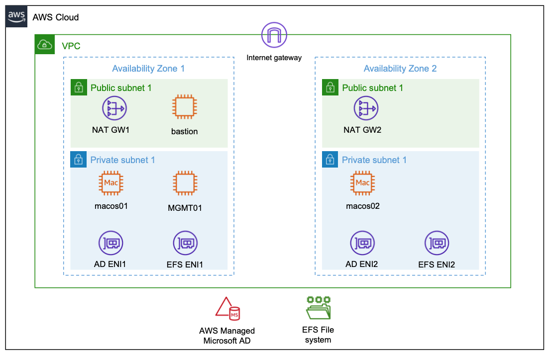
The following diagram shows the architecture rolled out in the context of this blog.

Architecture Diagram. A detailed description is featured in the blog text.

Compute Layer

The compute layer consists of two EC2 Mac instances running in isolated private subnets in different Availability Zones. In a production setup, these instances are provisioned with every necessary tool and software needed by developers to build and test their code for Apple platforms. Provisioning can be accomplished by creating custom Amazon Machine Images (AMIs) for the EC2 Mac instances or by bootstrapping them with setup scripts. This post utilizes Amazon provided AMIs with macOS BigSur without custom software. Once setup, developers gain command line access to the instances via SSH and utilize them as remote development environments.

Storage Layer

The architecture promotes the decoupling of compute and storage so that EC2 Mac instances can be updated with new OS and/or software versions without affecting the developer experience or data. Home directories reside on a highly available Amazon EFS file system, and they can be consistently accessed from all EC2 Mac instances. From a user perspective, any two EC2 Mac instances are alike, in that the user experiences the same configuration and environment (e.g., shell configurations such as .zshrc, VSCode remote extensions .vscode-server, or other tools and configurations installed within the user’s home directory). The file system is exposed to the private subnets via redundant mount target ENIs and persistently mounted on the Mac instances.

Identity Layer

For centralized user and access management, all instances in the architecture are part of a common Active Directory domain based on AWS Managed Microsoft AD. This is exposed via redundant ENIs to the private subnets containing the Mac instances.

To manage and configure the Active Directory domain, a Windows Instance (MGMT01) is deployed. For this post, we will connect to this instance for setting up Active Directory users. Note: other than that, this instance is not required for operating the solution, and it can be shut down both for reasons of cost efficiency and security.

Access Layer

The access layer constitutes the entry and exit point of the setup. For this post, it is comprised of an internet-facing bastion host connecting authorized Active Directory users to the Mac instances, as well as redundant NAT gateways providing outbound internet connectivity.

Depending on customer requirements, the access layer can be realized in various ways. For example, it can provide access to customer on-premises networks by using AWS Direct Connect or AWS Virtual Private Network (AWS VPN), or to services in different Virtual Private Cloud (VPC) networks by using AWS PrivateLink. This means that you can integrate your Mac development environment with pre-existing development-related services, such as source code and software repositories or build and test services.

Prerequisites

We utilize AWS CloudFormation to automatically deploy the entire setup in the preceding description. All templates and code can be obtained from the blog’s GitHub repository. To complete the setup, you need

Warning: Deploying this example will incur AWS service charges of at least $50 due to the fact that EC2 Mac instances can only be released 24 hours after allocation.

Solution Deployment

In this section, we provide a step-by-step guide for deploying the solution. We will mostly rely on AWS CLI and shell scripts provided along with the CloudFormation templates and use the AWS Management Console for checking and verification only.

1. Get the Code: Obtain the CloudFormation templates and all relevant scripts and assets via git:

git clone https://github.com/aws-samples/ec2-mac-remote-dev-env.git
cd ec2-mac-remote-dev-env
git submodule init 
git submodule update

2. Create an Amazon Simple Storage Service (Amazon S3) deployment bucket and upload assets for deployment: CloudFormation templates and other assets are uploaded to this bucket in order to deploy them. To achieve this, run the upload.sh script in the repository root, accepting the default bucket configuration as suggested by the script:

./upload.sh

3. Create an SSH Keypair for admin Access: To access the instances deployed by CloudFormation, create an SSH keypair with name mac-admin, and then import it with EC2:

ssh-keygen -f ~/.ssh/mac-admin
aws ec2 import-key-pair \
    --key-name "mac-admin" \
    --public-key-material fileb://~/.ssh/mac-admin.pub

4. Create CloudFormation Parameters file: Initialize the json file by copying the provided template parameters-template.json :

cp parameters-template.json parameters.json

Substitute the following placeholders:

a. <YourS3BucketName>: The unique name of the S3 bucket you created in step 2.

b. <YourSecurePassword>: Active Directory domain admin password. This must be 8-32 characters long and can contain numbers, letters and symbols.

c. <YourMacOSAmiID>: We used the latest macOS BigSur AMI at the time of writing with AMI ID ami-0c84d9da210c1110b in the us-east-2 Region. You can obtain other AMI IDs for your desired AWS Region and macOS version from the console.

d. <MacHost1ID> and <MacHost2ID>: See the next step 5. on how to allocate Dedicated Hosts and obtain the host IDs.

5. Allocate Dedicated Hosts: EC2 Mac Instances run on Dedicated Hosts. Therefore, prior to being able to deploy instances, Dedicated Hosts must be allocated. We utilize us-east-2 as the target Region, and we allocate the hosts in the Availability Zones us-east-2b and us-east-2c:

aws ec2 allocate-hosts \
    --auto-placement off \
    --region us-east-2 \
    --availability-zone us-east-2b \
    --instance-type mac1.metal \
    --quantity 1 \
    --tag-specifications 'ResourceType=dedicated-host,Tags=[{Key=Name,Value=MacHost1}]'

aws ec2 allocate-hosts \
    --auto-placement off \
    --region us-east-2 \
    --availability-zone us-east-2c \
    --instance-type mac1.metal \
    --quantity 1 \
    --tag-specifications 'ResourceType=dedicated-host,Tags=[{Key=Name,Value=MacHost2}]'

Substitute the host IDs returned from those commands in the parameters.json file as instructed in the previous step 5.

6. Deploy the CloudFormation Stack: To deploy the stack with the name ec2-mac-remote-dev-env, run the provided sh script as follows:

./deploy.sh ec2-mac-remote-dev-env

Stack deployment can take up to 1.5 hours, which is due to the Microsoft Managed Active Directory, the Windows MGMT01 instance, and the Mac instances being created sequentially. Check the CloudFormation Console to see whether the stack finished deploying. In the console, under Stacks, select the stack name from the preceding code (ec2-mac-remote-dev-env), and then navigate to the Outputs Tab. Once finished, this will display the public DNS name of the bastion host, as well as the private IPs of the Mac instances. You need this information in the upcoming section in order to connect and test your setup.

Solution Test

Now you can log in and explore the setup. We will start out by creating a developer account within Active Directory and configure an SSH key in order for it to grant access.

Create an Active Directory User

Create an SSH Key for the Active Directory User and configure SSH Client

First, we create a new SSH key for the developer Active Directory user. Utilize OpenSSH CLI,

ssh-keygen -f ~/.ssh/mac-developer

Furthermore, utilizing the connection information from the CloudFormation output, setup your ~/.ssh/config to contain the following entries, where $BASTION_HOST_PUBLIC_DNS, $MAC1_PRIVATE_IP and $MAC2_PRIVATE_IP must be replaced accordingly:

Host bastion
  HostName $BASTION_HOST_PUBLIC_DNS
  User ec2-user
  IdentityFile ~/.ssh/mac-admin

Host bastion-developer
  HostName $BASTION_HOST_PUBLIC_DNS
  User developer
  IdentityFile ~/.ssh/mac-developer

Host macos1
  HostName $MAC1_PRIVATE_IP
  ProxyJump %r@bastion-developer
  User developer
  IdentityFile ~/.ssh/mac-developer

Host macos2
  HostName $MAC2_PRIVATE_IP
  ProxyJump %r@bastion-developer
  User developer
  IdentityFile ~/.ssh/mac-developer

As you can see from this configuration, we set up both SSH keys created during this blog. The mac-admin key that you created earlier provides access to the privileged local ec2-user account, while the mac-developer key that you just created grants access to the unprivileged AD developer account. We will create this next.

Login to the Windows MGMT Instance and setup a developer Active Directory account

Now login to the bastion host, forwarding port 3389 to the MGMT01 host in order to gain Remote Desktop Access to the Windows management instance:

ssh -L3389:mgmt01:3389 bastion

While having this connection open, launch your Remote Desktop Client and connect to localhost with Username admin and password as specified earlier in the CloudFormation parameters. Once connected to the instance, open Control Panel>System and Security>Administrative Tools and click Active Directory Users and Computers. Then, in the appearing window, enable View>Advanced Features. If you haven’t changed the Active Directory domain name explicitly in CloudFormation, then the default domain name is example.com with corresponding NetBIOS Name example. Therefore, to create a new user for that domain, select Active Directory Users and Computers>example.com>example>Users, and click Create a new User. In the resulting wizard, set the Full name and User logon name fields to developer, and proceed to set a password to create the user. Once created, right-click on the developer user, and select Properties>Attribute Editor. Search for the altSecurityIdentities property, and copy-paste the developer public SSH key (contained in ~/.ssh/mac-developer.pub) into the Value to add field, click Add, and then click OK. In the Properties window, save your changes by clicking Apply and OK. The following figure illustrates the process just described:

Screenshot from the Windows Management instance depicting the creation of the Active Directory user. A detailed description of this process is contained in the blog text.

Connect to the EC2 Mac instances

Now that the developer account is setup, you can connect to either of the two EC2 Mac instances from your local machine with the Active Directory account:

ssh macos1

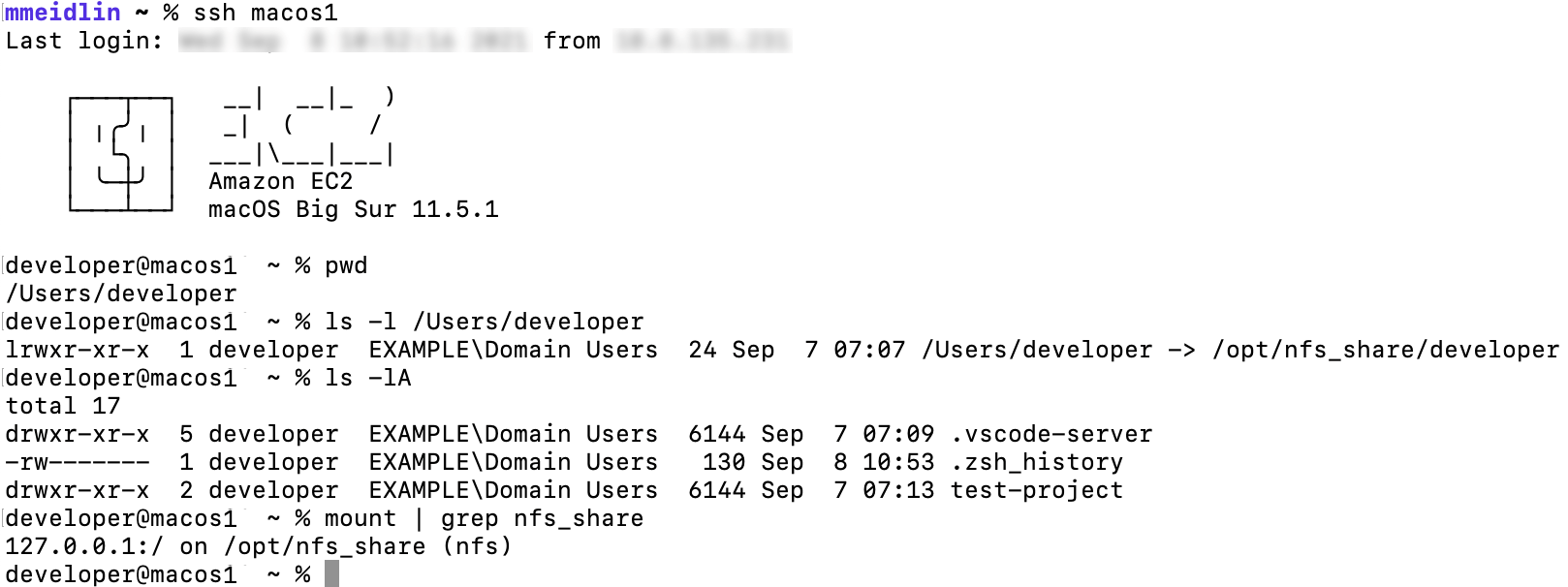
When you connect via the preceding command, your local machine first establishes an SSH connection to the bastion host which authorizes the request against the key we just stored in Active Directory. Upon success, the bastion host forwards the connection to the macos1 instance, which again authorizes against Active Directory and launches a  terminal session upon success. The following figure illustrates the login with the macos1 instances, showcasing both the integration with AD (EXAMPLE\Domain Users group membership) as well as with the EFS share, which is mounted at /opt/nfsshare and symlinked to the developer’s home directory.

Screenshot from a terminal window after logging into the macos1 instance. Instructions for doing this are included in the blog text.

Likewise, you can create folders and files in the developer’s home directory such as the test-project folder depicted in the screenshot.

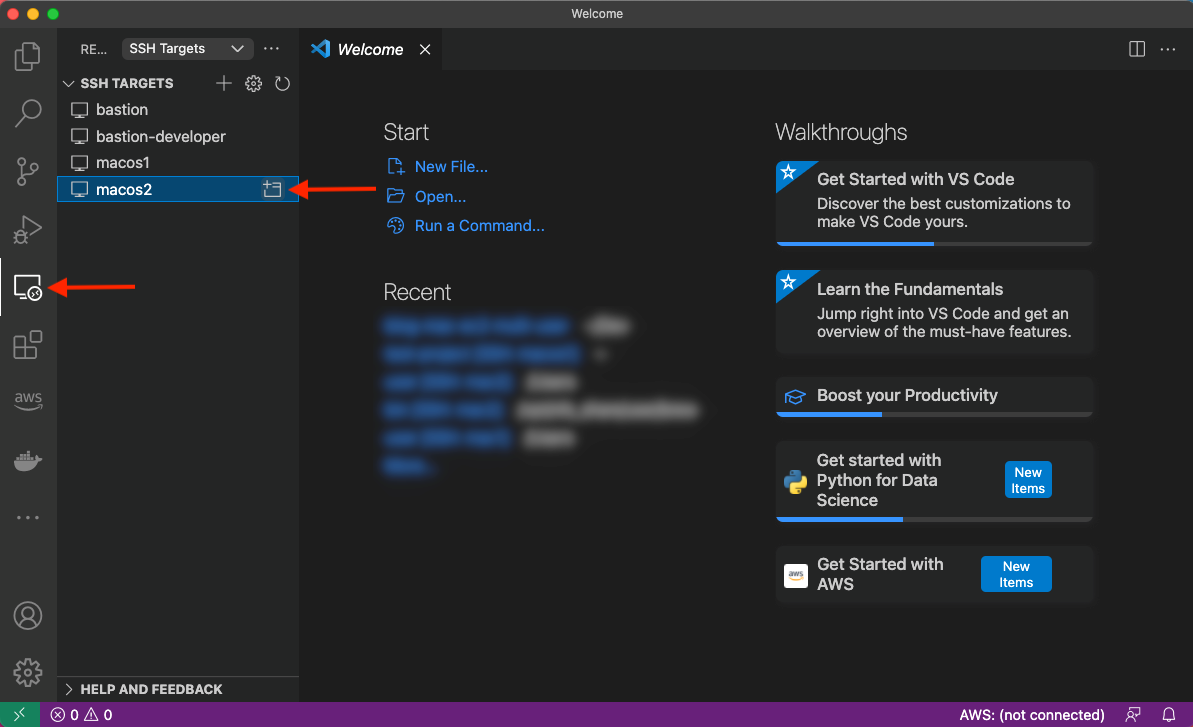
Lastly, let’s utilize VS Code’s remote plugin and connect to the other macos2 instance. Select the Remote Explorer on the left-hand pane and click to open the macos2 host as shown in the following screenshot:

Screenshot depicting how to connect to the macos2 instance using the VSCode Remote SSH extension.

A new window will be opened with the context of the remote server, as shown in the next figure. As you can see, we have access to the same files seen previously on the macos1 host.

Screenshot showing VSCode UI once connected to the macos2 instance.

Cleanup

From the repository root, run the provided destroy.sh script in order to destroy all resources created by CloudFormation, specifying the stack name as input parameter:

./destroy.sh ec2-mac-remote-dev-env

Check the CloudFormation Console to confirm that the stack and its resources are properly deleted.

Lastly, in the EC2 Console, release the dedicated Mac Hosts that you allocated in the beginning. Notice that this is only possible 24 hours after allocation.

Summary

This post has shown how EC2 Mac instances can be set up as remote development environments, thereby allowing developers to create software for Apple platforms regardless of their local hardware and software setup. Aside from increased flexibility and maintainability, this setup also saves cost because multiple developers can work interactively with the same EC2 Mac instance. We have rolled out an architecture that integrates EC2 Mac instances with AWS Directory Services for centralized user and access management as well as Amazon EFS to store developer home directories in a durable and highly available manner. This has resulted in an architecture where instances can easily be added, removed, or updated without affecting developer workflow. Now, irrespective of your client machine, you are all set to start coding with your local editor while leveraging EC2 Mac instances in the AWS Cloud to provide you with a macOS environment! To get started and learn more about EC2 Mac instances, please visit the product page.

Monitoring delay of AWS Batch jobs in transit before execution

Post Syndicated from Emma White original https://aws.amazon.com/blogs/compute/monitoring-delay-of-aws-batch-jobs-in-transit-before-execution/

This post is written by Nikhil Anand, Solutions Architect 

AWS Batch enables developers, scientists, and engineers to easily and efficiently run hundreds of thousands of batch processing jobs on AWS. With AWS Batch you no longer have to install and manage batch computing software or server clusters used to run your jobs. This lets you focus on analyzing results and solving problems, not managing infrastructure. When you use AWS Batch, in the job lifetime, a job goes through several states. When creating a compute environment to run the Batch jobs and submit Batch jobs, a settings misconfiguration could cause the job to get stuck in a transit state. This means the job will not proceed to the desired RUNNING state – a common issue faced by most customers.

If your compute environment contains compute resources, but your jobs don’t progress beyond the RUNNABLE state, then something is preventing the jobs from being placed on a compute resource. There are various reasons why a job could remain in the RUNNABLE state. The usual call to action is referring the troubleshooting documentation in order to fix the issue. Similarly, if your job is dependent on another job, then the job would stay in the PENDING state.

However, if you have scheduled actions to be completed with Batch jobs, or if you do not have any mechanism monitoring the jobs, then your jobs might stay in any of the transit states if left unattended. You may end up continuing forward, unaware that your job has yet to run. Eventually, when you see the jobs not progressing beyond the RUNNABLE or PENDING state, you miss the task that the job was expected to do in the given timeframe. This can result in additional time and effort troubleshooting the stuck job.

To prevent this accidental avoidance or lack of in-transit job monitoring, this post provides a monitoring solution for jobs in transit (from the SUBMITTED to the RUNNING state) in AWS Batch.

You can configure a threshold monitoring duration for your jobs so that if a job stays in SUBMITTED/PENDING/RUNNABLE longer than that, then you get a notification. For example, you might have a job that you would want to proceed to the RUNNING state in approximately 15 minutes since the job submission. Sometimes a slight misconfiguration can cause the job to get stuck in RUNNABLE indefinitely. In that case, you can set a threshold of 15 minutes. Or, suppose you have a job that is dependent on the other job that is stuck in processing. In these situations, once the specified duration is crossed, you are notified about your job staying in transit beyond your defined threshold status.

The solution is deployed by using AWS CloudFormation.

Overview of solution

The solution creates an Amazon CloudWatch Events rule that triggers an AWS Lambda function on a schedule. Then, the Lambda function checks every job in transit for more than ‘X’ seconds on all compute environments since the job submission. Specify your own value for ‘X’ when you launch the AWS CloudFormation stack. The solution consists of the following components created via CloudFormation:

  • An Amazon CloudWatch event rule to monitor the submitted jobs in Batch using the target Lambda function
  • An AWS Lambda function with the logic to monitor the submitted jobs and trigger Amazon Simple Notification Service (Amazon SNS) notifications
  • A Lambda execution AWS Identity and Access Management (IAM) role
  • An Amazon SNS topic to be subscribed by end users in order to be notified about the submitted jobs

The solution components and workflow.

Prerequisites

For this walkthrough, you should have the following prerequisites:

Walkthrough

To provision the necessary solution components, use this CloudFormation template. 

  1. While launching the CloudFormation stack, you will be asked to input the following information in addition to the CloudFormation stack name:
    1. The upper threshold (in seconds) for the jobs to stay in the transit state
    2. The evaluation period after which the Lambda runs periodically
    3. The email ID to get notifications after the job stays in the transit state for the defined threshold value.

pecify parameter values during CloudFormation stack launch

  1. Once the stack is created, the following resources will be provisioned – SNS topic, CloudWatch Events rule, Lambda function, Lambda invoke permissions, and Lambda execution role. View it in the ‘Resources’ tab of your CloudFormation stack.

Successful creation of the CloudFormation stack

  1. After the stack is created, the email ID you entered in step III above will receive an email from Amazon SNS in order to confirm the Amazon SNS subscription.

Subscription confirmation email that you receive on the specified email ID.

Click Confirm subscription in the email.

Subscription confirmed.

  1. Based on the customer’s inputs during stack launch, a Lambda function will be periodically invoked to look out for Batch jobs stuck in the RUNNABLE state for the defined threshold.
  2. An Amazon SNS notification is sent out at the evaluation periods with the job IDs of the jobs that have stayed stuck in the RUNNABLE state.

Verifying the solution

Launch your monitoring solution by using the CloudFormation template. Once the stack creation is complete, I get an email to subscribe to the SNS topic. Then, I subscribe to the SNS topic.

Click to launch Stack. 

Submit a job in AWS Batch by using console, CLI, or SDK. To test the solution, submit a job, Job1, to a job queue associated with a compute environment with no public subnets. Compute resources require access in order to communicate with the Amazon ECS service endpoint. This can be done through an interface VPC endpoint or your compute resources having public IP addresses. Since the compute environment was configured to only have a private subnet, Job1 will not proceed from the RUNNABLE state. Similarly, submit another job, Job2, and during submission add a dependency of Job1 on Job2. Therefore, Job2 will not proceed from the PENDING state. Thus, creating a sample space wherein two jobs will be stuck in transit.

AWS Batch jobs submitted and in transit.

Based on the CloudFormation template inputs, you will get notified on the subscribed Email ID when the job stays in transit for more than ‘X’ seconds (the input provided during stack launch).

otification received for the jobs that stayed in transit longer than expected.

Modifications

The Lambda function uses the ListJobs API call. The maximum number of results is returned by ListJobs in paginated output. Therefore, if you are submitting many jobs, then you must modify the Lambda function to fetch more results from the initial response of the call by using the nextToken response element. Use this nextToken element and iterate through in a loop to keep fetching the paginated results until there are no further nextToken elements present.

Cleaning up

To avoid incurring future charges, delete the resources. You can delete the CloudFormation stack that will clean up every resource that it provisioned for the monitoring solution.

Conclusion

This solution lets you detect AWS Batch jobs that remain in the transit state longer than expected. It provides you with an efficient way to monitor your Batch jobs. If the jobs stay in the RUNNABLE/PENDING/SUBMITTED state for a significant amount of time, then it is indicative of potential misconfiguration with either the compute environment setup, or with the job parameters that were passed during the job submission. An early notification around the issue can help you troubleshoot the misconfigurations early on and take subsequent actions.

If you have multiple jobs that remain in the RUNNABLE state and you realize that they will not proceed further to the RUNNING state due to a misconfiguration, then you can shut down all RUNNABLE jobs by using a simple bash script.

For additional references regarding troubleshooting RUNNABLE jobs in AWS Batch, refer to the suggested Knowledge Center article and the troubleshooting documentation.

Optimizing Apache Flink on Amazon EKS using Amazon EC2 Spot Instances

Post Syndicated from Emma White original https://aws.amazon.com/blogs/compute/optimizing-apache-flink-on-amazon-eks-using-amazon-ec2-spot-instances/

This post is written by Kinnar Sen, Senior EC2 Spot Specialist Solutions Architect

Apache Flink is a distributed data processing engine for stateful computations for both batch and stream data sources. Flink supports event time semantics for out-of-order events, exactly-once semantics, backpressure control, and optimized APIs. Flink has connectors for third-party data sources and AWS Services, such as Apache Kafka, Apache NiFi, Amazon Kinesis, and Amazon MSK. Flink can be used for Event Driven (Fraud Detection), Data Analytics (Ad-Hoc Analysis), and Data Pipeline (Continuous ETL) applications. Amazon Elastic Kubernetes Service (Amazon EKS) is the chosen deployment option for many AWS customers for Big Data frameworks such as Apache Spark and Apache Flink. Flink has native integration with Kubernetes allowing direct deployment and dynamic resource allocation.

In this post, I illustrate the deployment of scalable, highly available (HA), resilient, and cost optimized Flink application using Kubernetes via Amazon EKS and Amazon EC2 Spot Instances (Spot). Learn how to save money on big data streaming workloads by implementing this solution.

Overview

Amazon EC2 Spot Instances

Amazon EC2 Spot Instances let you take advantage of spare EC2 capacity in the AWS Cloud and are available at up to a 90% discount compared to On-Demand Instances. Spot Instances receive a two-minute warning when these instances are about to be reclaimed by Amazon EC2. There are many graceful ways to handle the interruption. Recently EC2 Instance rebalance recommendation has been added to send proactive notifications when a Spot Instance is at elevated risk of interruption. Spot Instances are a great way to scale up and increase throughput of Big Data workloads and has been adopted by many customers.

Apache Flink and Kubernetes

Apache Flink is an adaptable framework and it allows multiple deployment options and one of them being Kubernetes. Flink framework has a couple of key building blocks.

  • Job Client submits the job in form of a JobGraph to the Job Manager.
  • Job Manager plays the role of central work coordinator which distributes the job to the Task Managers.
  • Task Managers are the worker component, which runs the operators for source, transformations and sinks.
  • External components which are optional such as Resource Provider, HA Service Provider, Application Data Source, Sinks etc., and this varies with the deployment mode and options.

Image shows Flink application deployment architecture with Job Manager, Task Manager, Scheduler, Data Flow Graph, and client.

Flink supports different deployment (Resource Provider) modes when running on Kubernetes. In this blog we will use the Standalone Deployment mode, as we just want to showcase the functionality. We recommend first-time users however to deploy Flink on Kubernetes using the Native Kubernetes Deployment.

Flink can be run in different modes such as Session, Application, and Per-Job. The modes differ in cluster lifecycle, resource isolation and execution of the main() method. Flink can run jobs on Kubernetes via Application and Session Modes only.

  • Application Mode: This is a lightweight and scalable way to submit an application on Flink and is the preferred way to launch application as it supports better resource isolation. Resource isolation is achieved by running a cluster per job. Once the application shuts down all the Flink components are cleaned up.
  • Session Mode: This is a long running Kubernetes deployment of Flink. Multiple applications can be launched on a cluster and the applications competes for the resources. There may be multiple jobs running on a TaskManager in parallel. Its main advantage is that it saves time on spinning up a new Flink cluster for new jobs, however if one of the Task Managers fails it may impact all the jobs running on that.

Amazon EKS

Amazon EKS is a fully managed Kubernetes service. EKS supports creating and managing Spot Instances using Amazon EKS managed node groups following Spot best practices. This enables you to take advantage of the steep savings and scale that Spot Instances provide for interruptible workloads. EKS-managed node groups require less operational effort compared to using self-managed nodes. You can learn more in the blog “Amazon EKS now supports provisioning and managing EC2 Spot Instances in managed node groups.”

Apache Flink and Spot

Big Data frameworks like Spark and Flink are distributed to manage and process high volumes of data. Designed for failure, they can run on machines with different configurations, inherently resilient and flexible. Spot Instances can optimize runtimes by increasing throughput, while spending the same (or less). Flink can tolerate interruptions using restart and failover strategies.

Fault Tolerance

Fault tolerance is implemented in Flink with the help of check-pointing the state. Checkpoints allow Flink to recover state and positions in the streams. There are two per-requisites for check-pointing a persistent data source (Apache Kafka, Amazon Kinesis) which has the ability to replay data and a persistent distributed storage to store state (Amazon Simple Storage Service (Amazon S3), HDFS).

Cost Optimization

Job Manager and Task Manager are key building blocks of Flink. The Task Manager is the compute intensive part and Job Manager is the orchestrator. We would be running Task Manager on Spot Instances and Job Manager on On Demand Instances.

Scaling

Flink supports elastic scaling via Reactive Mode, Task Managers can be added/removed based on metrics monitored by an external service monitor like Horizontal Pod Autoscaling (HPA). When scaling up new pods would be added, if the cluster has resources they would be scheduled it not then they will go in pending state. Cluster Autoscaler (CA) detects pods in pending state and new nodes will be added by EC2 Auto Scaling. This is ideal with Spot Instances as it implements elastic scaling with higher throughput in a cost optimized way.

Tutorial: Running Flink applications in a cost optimized way

In this tutorial, I review steps, which help you launch cost optimized and resilient Flink workloads running on EKS via Application mode. The streaming application will read dummy Stock ticker prices send to an Amazon Kinesis Data Stream by Amazon Kinesis Data Generator, try to determine the highest price within a per-defined window, and output will be written onto Amazon S3 files.

Image shows Flink application pipeline with data flowing from Amazon Kinesis Data Generator to Kinesis Data Stream, processed in Apache Flink and output being written in Amazon S3

The configuration files can be found in this github location. To run the workload on Kubernetes, make sure you have eksctl and kubectl command line utilities installed on your computer or on an AWS Cloud9 environment. You can run this by using an AWS IAM user or role that has the Administrator Access policy attached to it, or check the minimum required permissions for using eksctl. The Spot node groups in the Amazon EKS cluster can be launched both in a managed or a self-managed way, in this post I use the EKS Managed node group for Spot Instances.

Steps

When we deploy Flink in Application Mode it runs as a single application. The cluster is exclusive for the job. We will be bundling the user code in the Flink image for that purpose and upload in Amazon Elastic Container Registry (Amazon ECR). Amazon ECR is a fully managed container registry that makes it easy to store, manage, share, and deploy your container images and artifacts anywhere.

1. Build the Amazon ECR Image

  • Login using the following cmd and don’t forget to replace the AWS_REGION and AWS_ACCOUNT_ID with your details.

aws ecr get-login-password --region ${AWS_REGION} | docker login --username AWS —password-stdin ${ACCOUNT_ID}.dkr.ecr.${AWS_REGION}.amazonaws.com

  • Create a repository

aws ecr create-repository --repository-name flink-demo --image-scanning-configuration scanOnPush=true —region ${AWS_REGION}

  • Build the Docker image:

Download the Docker file. I am using multistage docker build here. The sample code is from Github’s Amazon Kinesis Data Analytics Java examples. I modified the code to allow checkpointing and change the sliding window interval. Build and push the docker image using the following instructions.

docker build --tag flink-demo .

  • Tag and Push your image to Amazon ECR

docker tag flink-demo:latest ${ACCOUNT_ID}.dkr.ecr.${AWS_REGION}.amazonaws.com/flink-demo:latest
docker push ${ACCOUNT_ID}.dkr.ecr.${AWS_REGION}.
amazonaws.com/flink-demo:latest

2. Create Amazon S3/Amazon Kinesis Access Policy

First, I must create an access policy to allow the Flink application to read/write from Amazon fFS3 and read Kinesis data streams. Download the Amazon S3 policy file from here and modify the <<output folder>> to an Amazon S3 bucket which you have to create.

  • Run the following to create the policy. Note the ARN.

aws iam create-policy --policy-name flink-demo-policy --policy-document file://flink-demo-policy.json

3. Cluster and node groups deployment

  • Create an EKS cluster using the following command:

eksctl create cluster –name= flink-demo --node-private-networking --without-nodegroup --asg-access –region=<<AWS Region>>

The cluster takes approximately 15 minutes to launch.

  • Create the node group using the nodeGroup config file. I am using multiple nodeGroups of different sizes to adapt Spot best practice of diversification.  Replace the <<Policy ARN>> string using the ARN string from the previous step.

eksctl create nodegroup -f managedNodeGroups.yml

  • Download the Cluster Autoscaler and edit it to add the cluster-name (flink-demo)

curl -LO https://raw.githubusercontent.com/kubernetes/autoscaler/master/cluster-autoscaler/cloudprovider/aws/examples/cluster-autoscaler-autodiscover.yaml

4. Install the Cluster AutoScaler using the following command:

kubectl apply -f cluster-autoscaler-autodiscover.yaml

  • Using EKS Managed node groups requires significantly less operational effort compared to using self-managed node group and enables:
    • Auto enforcement of Spot best practices.
    • Spot Instance lifecycle management.
    • Auto labeling of Pods.
  • eksctl has integrated amazon-ec2-instance-selector to enable auto selection of instances based on the criteria passed. This has multiple benefits
    • ‘instance diversification’ is implemented by enabling multiple instance types selection in the node group which works well with CA
    • Reduces manual effort of selecting the instances.
  • We can create node group manifests using ‘dryrun’ and then create node groups using that.

eksctl create cluster --name flink-demo --instance-selector-vcpus=2 --instance-selector-memory=4 --dry-run

eksctl create node group -f managedNodeGroups.yml

5. Create service accounts for Flink

$ kubectl create serviceaccount flink-service-account
$ kubectl create clusterrolebinding flink-role-binding-flink --clusterrole=edit --serviceaccount=default:flink-service-account

6. Deploy Flink

This install folder here has all the YAML files required to deploy a standalone Flink cluster. Run the install.sh file. This will deploy the cluster with a JobManager, a pool of TaskManagers and a Service exposing JobManager’s ports.

  • This is a High-Availability(HA) deployment of Flink with the use of Kubernetes high availability service.
  • The JobManager runs on OnDemand and TaskManager on Spot. As the cluster is launched in Application Mode, if a node is interrupted only one job will be restarted.
  • Autoscaling is enabled by the use of ‘Reactive Mode’. Horizontal Pod Autoscaler is used to monitor the CPU load and scale accordingly.
  • Check-pointing is enabled which allows Flink to save state and be fault tolerant.

Image shows the Flink dashboard highlighting checkpoints for a job

7. Create Amazon Kinesis data stream and send dummy data      

Log in to AWS Management Console and create a Kinesis data stream name ‘ExampleInputStream’. Kinesis Data Generator is used to send data to the data stream. The template of the dummy data can be found here. Once this sends data the Flink application starts processing.

Image shows Amazon Kinesis Data Generator console sending data to Kinesis Data Strea

Observations

Spot Interruptions

If there is an interruption then the Flick application will be restarted using check-pointed data. The JobManager will restore the job as highlighted in the following log. The node will be replaced automatically by the Managed Node Group.

mage shows logs from a Flink job highlighting job restart using checkpoints.

One will be able to observe the graceful restart in the Flink UI.

Image shows the Flink dashboard highlighting job restart after failure.

AutoScaling

You can observe the elastic scaling using logs. The number of TaskManagers in the Flink UI will also reflect the scaling state.

Image shows kubectl output showing status of HPA during scale-out

Cleanup

If you are trying out the tutorial, run the following steps to make sure that you don’t encounter unwanted costs.

  • Run the delete.sh file.
  • Delete the EKS cluster and the node groups:
    • eksctl delete cluster --name flink-demo
  • Delete the Amazon S3 Access Policy:
    • aws iam delete-policy --policy-arn <<POLICY ARN>>
  • Delete the Amazon S3 Bucket:
    • aws s3 rb --force s3://<<S3_BUCKET>>
  • Delete the CloudFormation stack related to Kinesis Data Generator named ‘Kinesis-Data-Generator-Cognito-User’
  • Delete the Kinesis Data Stream.

Conclusion

In this blog, I demonstrated how you can run Flink workloads on a Kubernetes Cluster using Spot Instances, achieving scalability, resilience, and cost optimization. To cost optimize your Flink based big data workloads you should start thinking about using Amazon EKS and Spot Instances.

Implementing interruption tolerance in Amazon EC2 Spot with AWS Fault Injection Simulator

Post Syndicated from Pranaya Anshu original https://aws.amazon.com/blogs/compute/implementing-interruption-tolerance-in-amazon-ec2-spot-with-aws-fault-injection-simulator/

This post is written by Steve Cole, WW SA Leader for EC2 Spot, and David Bermeo, Senior Product Manager for EC2.

On October 20, 2021, AWS released new functionality to the Amazon Fault Injection Simulator that supports triggering the interruption of Amazon EC2 Spot Instances. This functionality lets you test the fault tolerance of your software by interrupting instances on command. The triggered interruption will be preceded with a Rebalance Recommendation (RBR) and Instance Termination Notification (ITN) so that you can fully test your applications as if an actual Spot interruption had occurred.

In this post, we’ll provide two examples of how easy it has now become to simulate Spot interruptions and validate the fault-tolerance of an application or service. We will demonstrate testing an application through the console and a service via CLI.

Engineering use-case (console)

Whether you are building a Spot-capable product or service from scratch or evaluating the Spot compatibility of existing software, the first step in testing is identifying whether or not the software is tolerant of being interrupted.

In the past, one way this was accomplished was with an AWS open-source tool called the Amazon EC2 Metadata Mock. This tool let customers simulate a Spot interruption as if it had been delivered through the Instance Metadata Service (IMDS), which then let customers test how their code responded to an RBR or an ITN. However, this model wasn’t a direct plug-and-play solution with how an actual Spot interruption would occur, since the signal wasn’t coming from AWS. In particular, the method didn’t provide the centralized notifications available through Amazon EventBridge or Amazon CloudWatch Events that enabled off-instance activities like launching AWS Lambda functions or other orchestration work when an RBR or ITN was received.

Now, Fault Injection Simulator has removed the need for custom logic, since it lets RBR and ITN signals be delivered via the standard IMDS and event services simultaneously.

Let’s walk through the process in the AWS Management Console. We’ll identify an instance that’s hosting a perpetually-running queue worker that checks the IMDS before pulling messages from Amazon Simple Queue Service (SQS). It will be part of a service stack that is scaled in and out based on the queue depth. Our goal is to make sure that the IMDS is being polled properly so that no new messages are pulled once an ITN is received. The typical processing time of a message with this example is 30 seconds, so we can wait for an ITN (which provides a two minute warning) and need not act on an RBR.

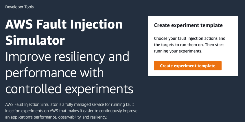
First, we go to the Fault Injection Simulator in the AWS Management Console to create an experiment.

AWS Fault Injection Simulator start screen in AWS Management console

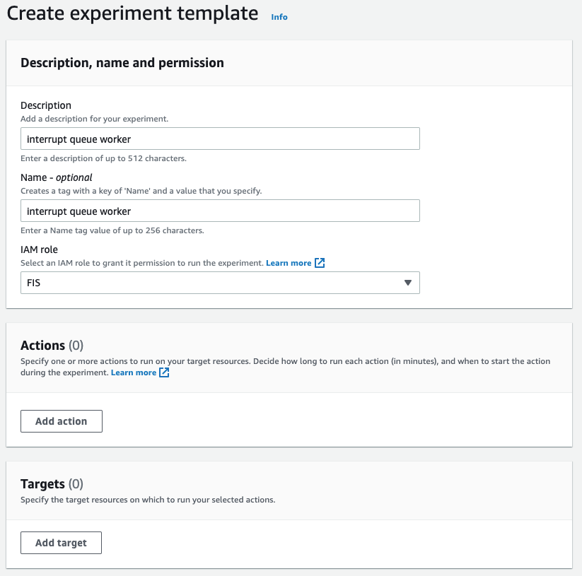
At the experiment creation screen, we start by creating an optional name (recommended for console use) and a description, and then selecting an IAM Role. If this is the first time that you’ve used Fault Injection Simulator, then you’ll need to create an IAM Role per the directions in the FIS IAM permissions documentation. I’ve named the role that we created ‘FIS.’ After that, I’ll select an action (interrupt) and identify a target (the instance).

Experiment template screen in AWS Management console with description “interrupt queue worker,” name “interrupt queue worker,” and IAM role “FIS.”

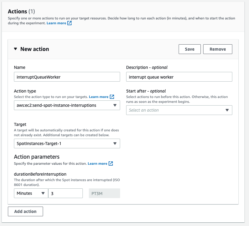
First, I name the action. The Action type I want is to interrupt the Spot Instance: aws:ec2:send-spot-instance-interruptions. In the Action parameters, we are given the option to set the duration. The minimum value here is two minutes, below which you will receive an error since Spot Instances will always receive a two minute warning. The advantage here is that, by setting the durationBeforeInterruption to a value above two minutes, you will get the RBR (an optional point for you to respond) and ITN (the actual two minute warning) at different points in time, and this lets you respond to one or both.

New action form in the create experiment template screen with name, description, action type and durationBeforeInterruption fields filled.

The target instance that we launched is depicted in the following screenshot. It is a Spot Instance that was launched as a persistent request with its interruption action set to ‘stop’ instead of ‘terminate.’ The option to stop a Spot Instance, introduced in 2020, will let us restart the instance, log in and retrieve logs, update code, and perform other work necessary to implement Spot interruption handling.

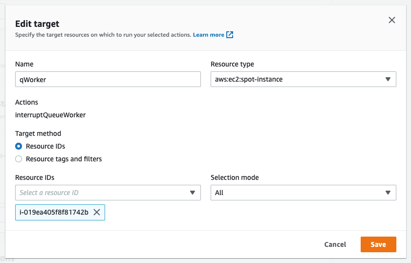
Now that an action has been defined, we configure the target. We have the option of naming the target, which we’ve done here to match the Name tagged on the EC2 instance ‘qWorker’. The target method we want to use here is Resource ID, and then we can either type or select the desired instance from a drop-down list. Selection mode will be ‘all’, as there is only one instance. If we were using tags, which we will in the next example, then we’d be able to select a count of instances, up to five, instead of just one.

Edit target form in the create experiment template screen with name, resource type, and resource id fields filled. Name is “qWorker,” Resource type is “aws:ec2:spot-Instance,” Target method is “Resource IDs” Resource IDs is “i-019ea405f8f81742b” and Selection mode is “All.”

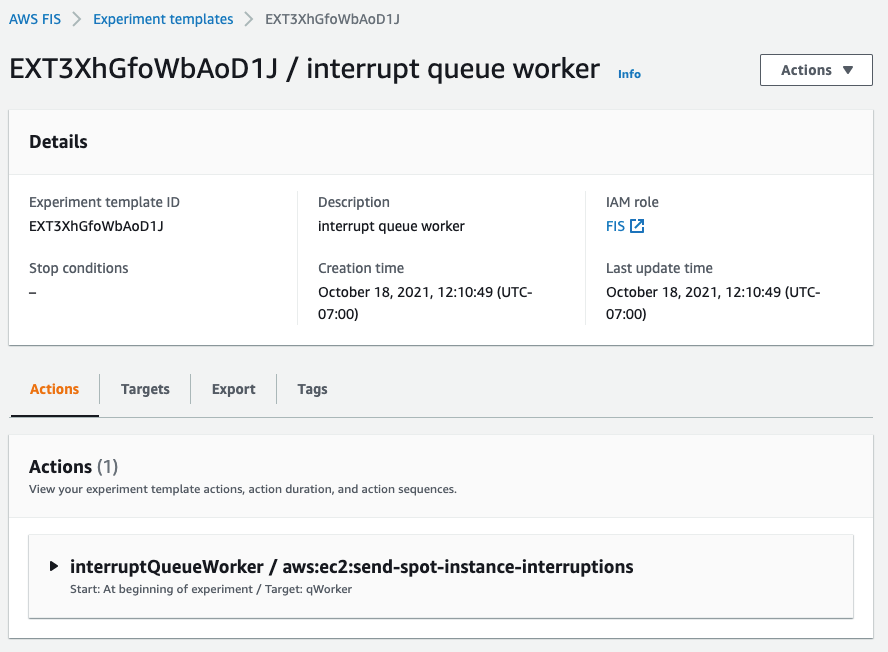
Once you’ve saved the Action, the Target, and the Experiment, then you’ll be able to begin the experiment by selecting the ‘Start from the Action’ menu at the top right of the screen.

Fault Injection Simulator Experiment template summary screen in the AWS Management console highlights experiment template ID, stop conditions, description, creation time, IAM role, and last update time.

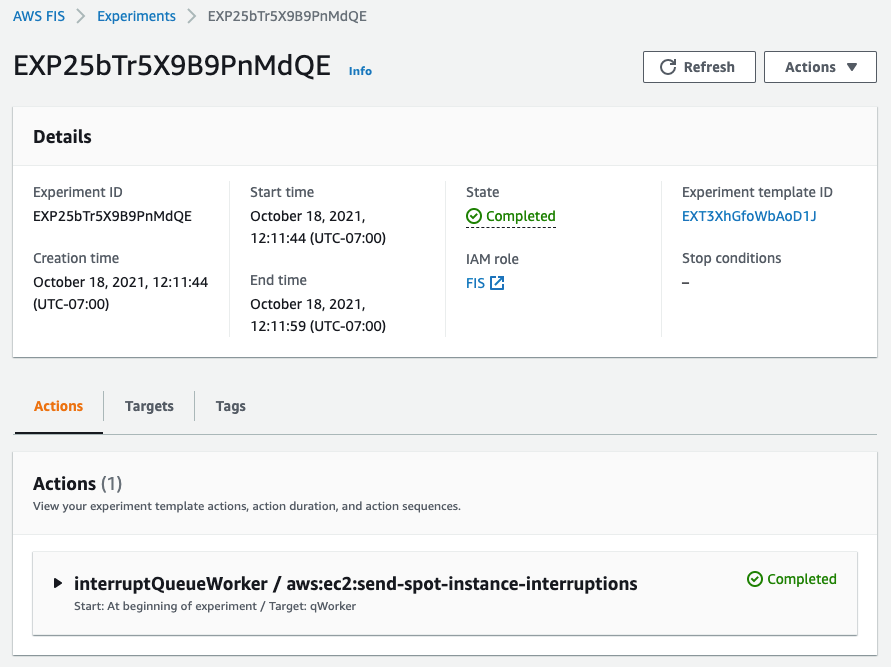
After the experiment starts, you’ll be able to observe its state by refreshing the screen. Generally, the process will take just seconds, and you should be greeted by the Completed state, as seen in the following screenshot.

Fault Injection Simulator Experiment summary screen in the AWS Management console shows status as “Completed.”

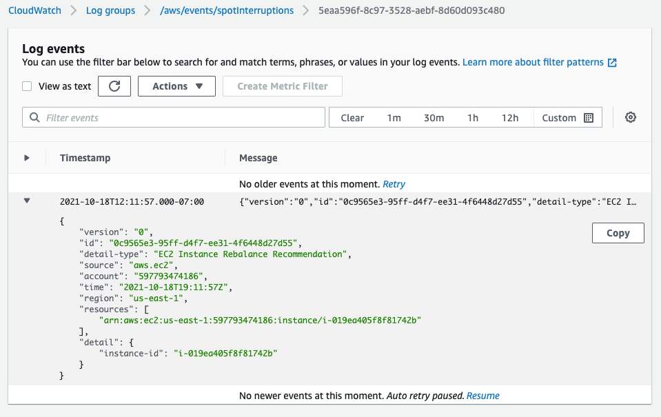
In the following screenshot, having opened an interruption log group created in CloudWatch Event Logs, we can see the JSON of the RBR.

CloudWatch Event Logs screen in the AWS Management Console with information on the EC2 Rebalance Recommendation.

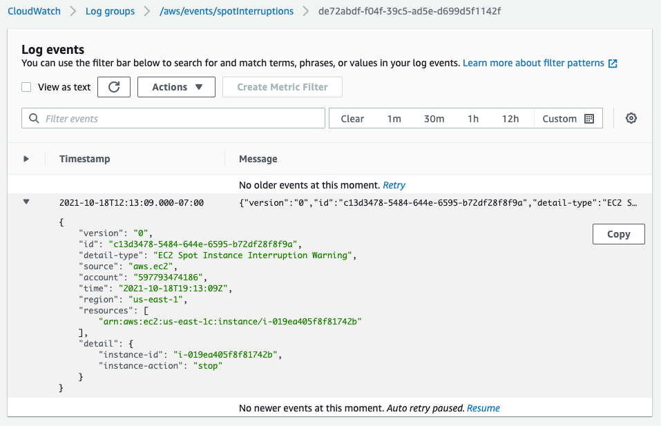
Two minutes later, we see the ITN in the same log group.

Cloudwatch Event Logs screen in the AWS Management console with information on the Instance Termination Notification.

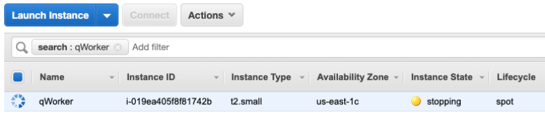
Another two minutes after the ITN, we can see the EC2 instance is in the process of stopping (or terminating, if you elect).

EC2 Instance List screen in the AWS Management console with information on the instance that is stopping.

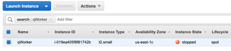
Shortly after the stop is issued by EC2, we can see the instance stopped. It would now be possible to restart the instance and view logs, make code changes, or do whatever you find necessary before testing again.

EC2 Instance List screen in the AWS Management console with information on the Instance that is stopped.

Now that our experiment succeeded in interrupting our Spot Instance, we can evaluate the performance of the code running on the instance. It should have completed the processing of any messages already retrieved at the ITN, and it should have not pulled any new messages afterward.

This experiment can be saved for later use, but it will require selecting the specific instance each time that it’s run. We can also re-use the experiment template by using tags instead of an instance ID, as we’ll show in the next example. This shouldn’t prove troublesome for infrequent experiments, and especially those run through the console. Or, as we did in our example, you can set the instance interruption behavior to stop (versus terminate) and re-use the experiment as long as that particular instance continues to exist. When the experiments get more frequent, it might be advantageous to automate the process, possibly as part of the test phase of a CI/CD pipeline. Doing this is programmatically possible through the AWS CLI or SDK.

Operations use-case (CLI)

Once the developers of our product validate the single-instance fault tolerance, indicating that the target workload is capable of running on Spot Instances, then the next logical step is to deploy the product as a service on multiple instances. This will allow for more comprehensive testing of the service as a whole, and it is a key process in collecting valuable information, such as performance data, response times, error rates, and other metrics to be used in the monitoring of the service. Once data has been collected on a non-interrupted deployment, it is then possible to use the Spot interruption action of the Fault Injection Simulator to observe how well the service can handle RBR and ITN while running, and to see how those events influence the metrics collected previously.

When testing a service, whether it is launched as instances in an Amazon EC2 Auto Scaling group, or it is part of one of the AWS container services, such as Amazon Elastic Container Service (Amazon ECS) or the Amazon Elastic Kubernetes Service (EKS), EC2 Fleet, Amazon EMR, or across any instances with descriptive tagging, you now have the ability to trigger Spot interruptions to as many as five instances in a single Fault Injection Simulator experiment.

We’ll use tags, as opposed to instance IDs, to identify candidates for interruption to interrupt multiple Spot Instances simultaneously. We can further refine the candidate targets with one or more filters in our experiment, for example targeting only running instances if you perform an action repeatedly.

In the following example, we will be interrupting three instances in an Auto Scaling group that is backing a self-managed EKS node group. We already know the software will behave as desired from our previous engineering tests. Our goal here is to see how quickly EKS can launch replacement tasks and identify how the service as a whole responds during the event. In our experiment, we will identify instances that contain the tag aws:autoscaling:groupName with a value of “spotEKS”.

The key benefit here is that we don’t need a list of instance IDs in our experiment. Therefore, this is a re-usable experiment that can be incorporated into test automation without needing to make specific selections from previous steps like collecting instance IDs from the target Auto Scaling group.

We start by creating a file that describes our experiment in JSON rather than through the console:

{
    "description": "interrupt multiple random instances in ASG",
    "targets": {
        "spotEKS": {
            "resourceType": "aws:ec2:spot-instance",
            "resourceTags": {
                "aws:autoscaling:groupName": "spotEKS"
            },
            "selectionMode": "COUNT(3)"
        }
    },
    "actions": {
        "interrupt": {
            "actionId": "aws:ec2:send-spot-instance-interruptions",
            "description": "interrupt multiple instances",
            "parameters": {
                "durationBeforeInterruption": "PT4M"
            },
            "targets": {
            "SpotInstances": "spotEKS"
            }
        }
    },
    "stopConditions": [
        {
            "source": "none"
        }
    ],
    "roleArn": "arn:aws:iam::xxxxxxxxxxxx:role/FIS",
    "tags": {
        "Name": "multi-instance"
    }
}

Then we upload the experiment template to Fault Injection Simulator from the command-line.

aws fis create-experiment-template --cli-input-json file://experiment.json

The response we receive returns our template along with an ID, which we’ll need to execute the experiment.

{
    "experimentTemplate": {
        "id": "EXT3SHtpk1N4qmsn",
        ...
    }
}

We then execute the experiment from the command-line using the ID that we were given at template creation.

aws fis start-experiment --experiment-template-id EXT3SHtpk1N4qmsn

We then receive confirmation that the experiment has started.

{
    "experiment": {
        "id": "EXPaFhEaX8GusfztyY",
        "experimentTemplateId": "EXT3SHtpk1N4qmsn",
        "state": {
            "status": "initiating",
            "reason": "Experiment is initiating."
        },
        ...
    }
}

To check the status of the experiment as it runs, which for interrupting Spot Instances is quite fast, we can query the experiment ID for success or failure messages as follows:

aws fis get-experiment --id EXPaFhEaX8GusfztyY

And finally, we can confirm the results of our experiment by listing our instances through EC2. Here we use the following command-line before and after execution to generate pre- and post-experiment output:

aws ec2 describe-instances --filters\
 Name='tag:aws:autoscaling:groupName',Values='spotEKS'\
 Name='instance-state-name',Values='running'\
 | jq .Reservations[].Instances[].InstanceId | sort

We can then compare this to identify which instances were interrupted and which were launched as replacements.

< "i-003c8d95c7b6e3c63"
< "i-03aa172262c16840a"
< "i-02572fa37a61dc319"
---
> "i-04a13406d11a38ca6"
> "i-02723d957dc243981"
> "i-05ced3f71736b5c95"

Summary

In the previous examples, we have demonstrated through the console and command-line how you can use the Spot interruption action in the Fault Injection Simulator to ascertain how your software and service will behave when encountering a Spot interruption. Simulating Spot interruptions will help assess the fault-tolerance of your software and can assess the impact of interruptions in a running service. The addition of events can enable more tooling, and being able to simulate both ITNs and RBRs, along with the Capacity Rebalance feature of Auto scaling groups, now matches the end-to-end experience of an actual AWS interruption. Get started on simulating Spot interruptions in the console.

Implementing Auto Scaling for EC2 Mac Instances

Post Syndicated from Rick Armstrong original https://aws.amazon.com/blogs/compute/implementing-autoscaling-for-ec2-mac-instances/

This post is written by: Josh Bonello, Senior DevOps Architect, AWS Professional Services; Wes Fabella, Senior DevOps Architect, AWS Professional Services

Amazon Elastic Compute Cloud (Amazon EC2) is a web service that provides secure, resizable compute capacity in the cloud. The introduction of Amazon EC2 Mac now enables macOS based workloads to run in the AWS Cloud. These EC2 instances require Dedicated Hosts usage. EC2 integrates natively with Amazon CloudWatch to provide monitoring and observability capabilities.

In order to best leverage EC2 for dynamic workloads, it is a best practice to use Auto Scaling whenever possible. This will allow your workload to scale to demand, while keeping a minimal footprint during low activity periods. With Auto Scaling, you don’t have to worry about provisioning more servers to handle peak traffic or paying for more than you need.

This post will discuss how to create an Auto Scaling Group for the mac1.metal instance type. We will produce an Auto Scaling Group, a Launch Template, a Host Resource Group, and a License Configuration. These resources will work together to produce the now expected behavior of standard instance types with Auto Scaling. At AWS Professional Services, we have implemented this architecture to allow the dynamic sizing of a compute fleet utilizing the mac1.metal instance type for a large customer. Depending on what should invoke the scaling mechanisms, this architecture can be easily adapted to integrate with other AWS services, such as Elastic Load Balancers (ELB). We will provide Terraform templates as part of the walkthrough. Please take special note of the costs associated with running three mac1.metal Dedicated Hosts for 24 hours.

How it works

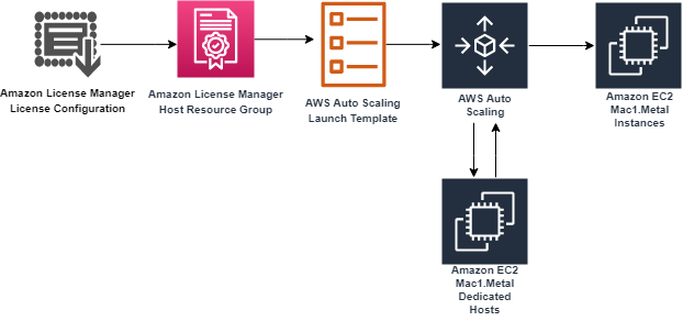
First, we will begin in AWS License Manager and create a License Configuration. This License Configuration will be associated with an Amazon Machine Image (AMI), and can be associated with multiple AMIs. We will utilize this License Configuration as a parameter when we create a Host Resource Group. As part of defining the Launch Template, we will be referencing our Host Resource Group. Then, we will create an Auto Scaling Group based on the Launch Template.

Example flow of License Manager, AWS Auto Scaling, and EC2 Instances and their relationship to each other.

The License Configuration will control the software licensing parameters. Normally, License Configurations are used for software licensing controls. In our case, it is only a required element for a Host Resource Group, and it handles nothing significant in our solution.

The Host Resource Group will be responsible for allocating and deallocating the Dedicated Hosts for the Mac1 instance family. An available Dedicated Host is required to launch a mac1.metal EC2 instance.

The Launch Template will govern many aspects to our EC2 Instances, including AWS Identity and Access Management (IAM) Instance Profile, Security Groups, and Subnets. These will be similar to typical Auto Scaling Group expectations. Note that, in our solution, we will use Tenancy Host Resource Group as our compute source.

Finally, we will create an Auto Scaling Group based on our Launch Template. The Auto Scaling Group will be the controller to signal when to create new EC2 Instances, create new Dedicated Hosts, and similarly terminate EC2 Instances. Unutilized Dedicated Hosts will be tracked and terminated by the Host Resource Group.

Limits

Some limits exist for this solution. To deploy this solution, a Service Quota Increase must be submitted for mac1.metal Dedicated Hosts, as the default quota is 0. Deploying the solution without this increase will result in failures when provisioning the Dedicated Hosts for the mac1.metal instances.

While testing scale-in operations of the auto scaling group, you might find that Dedicated Hosts are in “Pending” state. Mac1 documentation says “When you stop or terminate a Mac instance, Amazon EC2 performs a scrubbing workflow on the underlying Dedicated Host to erase the internal SSD, to clear the persistent NVRAM variables. If the bridgeOS software does not need to be updated, the scrubbing workflow takes up to 50 minutes to complete. If the bridgeOS software needs to be updated, the scrubbing workflow can take up to 3 hours to complete.” The Dedicated Host cannot be reused for a new scale-out operation until this scrubbing is complete. If you attempt a scale-in and a scale-out operation during testing, you might find more Dedicated Hosts than EC2 instances for your ASG as a result.

Auto Scaling Group features like dynamic scaling, health checking, and instance refresh can also cause similar side effects as a result of terminating the EC2 instances. These side effects will subside after 24 hours when a mac1 dedicate host can be released.

Building the solution

This walkthrough will utilize a Terraform template to automate the infrastructure deployment required for this solution. The following prerequisites should be met prior to proceeding with this walkthrough:

Before proceeding, note that the AWS resources created as part of the walkthrough have costs associated with them. Delete any AWS resources created by the walkthrough that you do not intend to use. Take special note that at the time of writing, mac1.metal Dedicated Hosts require a 24 minimum allocation time to align with Apple macOS EULA, and that mac1.metal EC2 instances are not charged separately, only the underlying Dedicated Hosts are.

Step 1: Deploy Dedicated Hosts infrastructure

First, we will do one-time setup for AWS License Manager to have the required IAM Permissions through the AWS Management Console. If you have already used License Manager, this has already been done for you. Click on “create customer managed license”, check the box, and then click on “Grant Permissions.”

AWS License Manager IAM Permissions Grant

To deploy the infrastructure, we will utilize a Terraform template to automate every component setup. The code is available at https://github.com/aws-samples/amazon-autoscaling-mac1metal-ec2-with-terraform. First, initialize your Terraform host. For this solution, utilize a local machine. For this walkthrough, we will assume the use of the us-west-2 (Oregon) AWS Region and the following links to help check resources will account for this.

terraform -chdir=terraform-aws-dedicated-hosts init

Initializing Terraform host and showing an example of expected output.

Then, we will plan our Terraform deployment and verify what we will be building before deployment.

terraform -chdir=terraform-aws-dedicated-hosts plan

In our case, we will expect a CloudFormation Stack and a Host Resource Group.

Planning Terraform template and showing an example of expected output.

Then, apply our Terraform deployment and verify via the AWS Management Console.

terraform -chdir=terraform-aws-dedicated-hosts apply -auto-approve

Applying Terraform template and showing an example of expected output.

Check that the License Configuration has been made in License Manager with a name similar to MyRequiredLicense.

Example of License Manager License after Terraform Template is applied.

Check that the Host Resource Group has been made in the AWS Management Console. Ensure that the name is similar to mac1-host-resource-group-famous-anchovy.

Example of Cloudformation Stack that is created, with License Manager Host Resource Group name pictured.

Note the host resource group name in the HostResourceGroup “Physical ID” value for the next step.

Step 2: Deploy mac1.metal Auto Scaling Group

We will be taking similar steps as in Step 1 with a new component set.

Initialize your Terraform State:

terraform -chdir=terraform-aws-ec2-mac init

Then, update the following values in terraform-aws-ec2-mac/my.tfvars:

vpc_id : Check the ID of a VPC in the account where you are deploying. You will always have a “default” VPC.

subnet_ids : Check the ID of one or many subnets in your VPC.

hint: use https://us-west-2.console.aws.amazon.com/vpc/home?region=us-west-2#subnets

security_group_ids : Check the ID of a Security Group in the account where you are deploying. You will always have a “default” SG.

host_resource_group_cfn_stack_name : Use the Host Resource Group Name value from the previous step.

Then, plan your deployment using the following:

terraform -chdir=terraform-aws-ec2-mac plan -var-file="my.tfvars"

Once we’re ready to deploy, utilize Terraform to apply the following:

terraform -chdir=terraform-aws-ec2-mac apply -var-file="my.tfvars" -auto-approve

Note, this will take three to five minutes to complete.

Step 3: Verify Deployment

Check our Auto Scaling Group in the AWS Management Console for a group named something like “ec2-native-xxxx”. Verify all attributes that we care about, including the underlying EC2.

Example of Autoscaling Group listing the EC2 Instances with mac1.metal instance type showing InService after Terraform Template is applied.

Check our Elastic Load Balancer in the AWS Management Console with a Tag key “Name” and the value of your Auto Scaling Group.

Check for the existence of our Dedicated Hosts in the AWS Management Console.

Step 4: Test Scaling Features

Now we have the entire infrastructure in place for an Auto Scaling Group to conduct normal activity. We will test with a scale-out behavior, then a scale-in behavior. We will force operations by updating the desired count of the Auto Scaling Group.

For scaling out, update the my.tfvars variable number_of_instances to three from two, and then apply our terraform template. We will expect to see one more EC2 instance for a total of three instances, with three Dedicated Hosts.

terraform -chdir=terraform-aws-ec2-mac apply -var-file="my.tfvars" -auto-approve

Then, take the steps in Step 3: Verify Deployment in order to check for expected behavior.

For scaling in, update the my.tfvars variable number_of_instances to one from three, and then apply our terraform template. We will expect your Auto Scaling Group to reduce to one active EC2 instance and have three Dedicated Hosts remaining until they are capable of being released 24 hours later.

terraform -chdir=terraform-aws-ec2-mac apply -var-file="my.tfvars" -auto-approve

Then, take the steps in Step 3: Verify Deployment in order to check for expected behavior.

Cleaning up

Complete the following steps in order to cleanup resources created by this exercise:

terraform -chdir=terraform-aws-ec2-mac destroy -var-file="my.tfvars" -auto-approve

This will take 10 to 12 minutes. Then, wait 24 hours for the Dedicated Hosts to be capable of being released, and then destroy the next template. We recommend putting a reminder on your calendar to make sure that you don’t forget this step.

terraform -chdir=terraform-aws-dedicated-hosts destroy -auto-approve

Conclusion

In this post, we created an Auto Scaling Group using mac1.metal instance types. Scaling mechanisms will work as expected with standard EC2 instance types, and the management of Dedicated Hosts is automated. This enables the management of macOS based application workloads to be automated based on the Well Architected patterns. Furthermore, this automation allows for rapid reactions to surges of demand and reclamation of unused compute once the demand is cleared. Now you can augment this system to integrate with other AWS services, such as Elastic Load Balancing, Amazon Simple Cloud Storage (Amazon S3), Amazon Relational Database Service (Amazon RDS), and more.

Review the information available regarding CloudWatch custom metrics to discover possibilities for adding new ways for scaling your system. Now we would be eager to know what AWS solution you’re going to build with the content described by this blog post! To get started with EC2 Mac instances, please visit the product page.

Deep Dive on Amazon EC2 VT1 Instances

Post Syndicated from Rick Armstrong original https://aws.amazon.com/blogs/compute/deep-dive-on-amazon-ec2-vt1-instances/

This post is written by:  Amr Ragab, Senior Solutions Architect; Bryan Samis, Principal Elemental SSA; Leif Reinert, Senior Product Manager

Introduction

We at AWS are excited to announce that new Amazon Elastic Compute Cloud (Amazon EC2) VT1 instances are now generally available in the US-East (N. Virginia), US-West (Oregon), Europe (Ireland), and Asia Pacific (Tokyo) Regions. This instance family provides dedicated video transcoding hardware in Amazon EC2 and offers up to 30% lower cost per stream as compared to G4dn GPU based instances or 60% lower cost per stream as compared to C5 CPU based instances. These instances are powered by Xilinx Alveo U30 media accelerators with up to eight U30 media accelerators per instance in the vt1.24xlarge. Each U30 accelerator comes with two XCU30 Zynq UltraScale+ SoCs, totaling 16 addressable devices in the vt1.24xlarge instance with H.264/H.265 Video Codec Units (VCU) cores.

Each U30 accelerator card comes with two XCU30 Zynq UltraScale+ SoCs

Currently, the VT1 family consists of three sizes, as summarized in the following:

Instance Type vCPUs RAM U30 accelerator cards Addressable XCU30 SoCs 
vt1.3xlarge 12 24 1 2
vt1.6xlarge 24 48 2 8
vt1.24xlarge 96 182 8 16

Each addressable XCU30 SoC device supports:

  • Codec: MPEG4 Part 10 H.264, MPEG-H Part 2 HEVC H.265
  • Resolutions: 128×128 to 3840×2160
  • Flexible rate control: Constant Bitrate (CBR), Variable Bitrate(VBR), and Constant Quantization Parameter(QP)
  • Frame Scan Types: Progressive H.264/H.265
  • Input Color Space: YCbCr 4:2:0, 8-bit per color channel.

The following table outlines the number of transcoding streams per addressable device and instance type:

Transcoding Each XCU30 SoC vt1.3xlarge vt1.6xlarge vt1.24xlarge
3840x2160p60 1 2 4 16
3840x2160p30 2 4 8 32
1920x1080p60 4 8 16 64
1920x1080p30 8 16 32 128
1280x720p30 16 32 64 256
960x540p30 24 48 92 384

Each XCU30 SoC can support the following stream densities: 1x 4kp60, 2x 4kp30, 4x 1080p60, 8x 1080p30, 16x 720p30

Customers with applications such as live broadcast, video conferencing and just-in-time transcoding can now benefit from a dedicated instance family devoted to video encoding and decoding with rescaling optimizations at the lowest cost per stream. This dedicated instance family lets customers run batch, real-time, and faster than real-time transcoding workloads.

Deployment and Quick Start

To get started, you launch a VT1 instance with prebuilt VT1 Amazon Machine Images (AMIs), available on the AWS Marketplace. However, if you have AMI hardening requirements or other requirements that require you to install the Xilinx software stack, you can reference the Xilinx Video SDK documentation for VT1.

The software stack utilizes a driver suite that is a combination of the driver stack as well as management and client tools. The following terminology will be used in this instance family:

  • XRT – Xilinx Runtime Library
  • XRM – Xilinx Runtime Management Library
  • XCDR – Xilinx Video Transcoding SDK
  • XMA – Xilinx Media Accelerator API and Samples
  • XOCL – Xilinx driver (xocl)

To run workloads directly on Amazon EC2 instances, you must load both the XRT and XRM stack. These are conveniently provided by loading the XCDR environment. To load the devices, run the following:

source /opt/xilinx/xcdr/setup.sh

With the output:

-----Source Xilinx U30 setup files-----
XILINX_XRT        : /opt/xilinx/xrt
PATH              : /opt/xilinx/xrt/bin:/usr/local/sbin:/sbin:/bin:/usr/sbin:/usr/bin:/root/bin
LD_LIBRARY_PATH   : /opt/xilinx/xrt/lib:
PYTHONPATH        : /opt/xilinx/xrt/python:
XILINX_XRM      : /opt/xilinx/xrm
PATH            : /opt/xilinx/xrm/bin:/opt/xilinx/xrt/bin:/usr/local/sbin:/sbin:/bin:/usr/sbin:/usr/bin:/root/bin
LD_LIBRARY_PATH : /opt/xilinx/xrm/lib:/opt/xilinx/xrt/lib:
Number of U30 devices found : 16  

Running Containerized Workloads on Amazon ECS and Amazon EKS

To help build AMIs for Amazon Linux2, Ubuntu 18/20, Amazon ECS and Amazon Elastic Kubernetes Service (Amazon EKS), we have provided a Github project in order to simplify the build process utilizing Packer:

https://github.com/aws-samples/aws-vt-baseami-pipeline

At the time of writing, Xilinx does not have an officially supported container runtime. However, it is possible to pass the specific devices in the docker run ... stanza, and in order to set this environment download this specific script. The following example is the output for vt1.24xlarge:

[ec2-user@ip-10-0-254-236 ~]$ source xilinx_aws_docker_setup.sh
XILINX_XRT : /opt/xilinx/xrt
PATH : /opt/xilinx/xrt/bin:/usr/local/bin:/usr/bin:/usr/local/sbin:/usr/sbin:/home/ec2-user/.local/bin:/home/ec2-user/bin
LD_LIBRARY_PATH  : /opt/xilinx/xrt/lib:
PYTHONPATH : /opt/xilinx/xrt/python:
XILINX_AWS_DOCKER_DEVICES : --device=/dev/dri/renderD128:/dev/dri/renderD128
--device=/dev/dri/renderD129:/dev/dri/renderD129
--device=/dev/dri/renderD130:/dev/dri/renderD130
--device=/dev/dri/renderD131:/dev/dri/renderD131
--device=/dev/dri/renderD132:/dev/dri/renderD132
--device=/dev/dri/renderD133:/dev/dri/renderD133
--device=/dev/dri/renderD134:/dev/dri/renderD134
--device=/dev/dri/renderD135:/dev/dri/renderD135
--device=/dev/dri/renderD136:/dev/dri/renderD136
--device=/dev/dri/renderD137:/dev/dri/renderD137
--device=/dev/dri/renderD138:/dev/dri/renderD138
--device=/dev/dri/renderD139:/dev/dri/renderD139
--device=/dev/dri/renderD140:/dev/dri/renderD140
--device=/dev/dri/renderD141:/dev/dri/renderD141
--device=/dev/dri/renderD142:/dev/dri/renderD142
--device=/dev/dri/renderD143:/dev/dri/renderD143
--mount type=bind,source=/sys/bus/pci/devices/0000:00:1d.0,target=/sys/bus/pci/devices/0000:00:1d.0 --mount type=bind,source=/sys/bus/pci/devices/0000:00:1e.0,target=/sys/bus/pci/devices/0000:00:1e.0

Once the devices have been enumerated, start the workload by running:

docker run -it $XILINX_AWS_DOCKER_DEVICES <image:tag>

Amazon EKS Setup

To launch an EKS cluster with VT1 instances, create the AMI from the scripts provided in the repo earlier.

https://github.com/aws-samples/aws-vt-baseami-pipeline

Once the AMI is created, launch an EKS cluster:

eksctl create cluster --region us-east-1 --without-nodegroup --version 1.19 \
       --zones us-east-1c,us-east-1d

Once the cluster is created, substitute the values for the cluster name, subnets, and AMI IDs in the following template.

apiVersion: eksctl.io/v1alpha5
kind: ClusterConfig

metadata:
  name: <cluster-name>
  region: us-east-1

vpc:
  id: vpc-285eb355
  subnets:
    public:
      endpoint-one:
        id: subnet-5163b237
      endpoint-two:
        id: subnet-baff22e5

managedNodeGroups:
  - name: vt1-ng-1d
    instanceType: vt1.3xlarge
    volumeSize: 200
    instancePrefix: vt1-ng-1d-worker
    ami: <ami-id>
    iam:
      withAddonPolicies:
        imageBuilder: true
        autoScaler: true
        ebs: true
        fsx: true
        cloudWatch: true
    ssh:
      allow: true
      publicKeyName: amrragab-aws
    subnets:
    - endpoint-one
    minSize: 1
    desiredCapacity: 1
    maxSize: 4
    overrideBootstrapCommand: |
      #!/bin/bash
      /etc/eks/bootstrap.sh <cluster-name>

Save this file, and then deploy the nodegroup.

eksctl create nodegroup -f vt1-managed-ng.yaml

Once deployed, apply the FPGA U30 device plugin. The daemonset container is available on the Amazon Elastic Container Registry (ECR) public gallery. You can also access the daemonset deployment file.

kubectl apply -f xilinx-device-plugin.yml

Confirm that the Xilinx U30 device(s) are seen by K8s API server and can be allocatable in your job.

Capacity:
  attachable-volumes-aws-ebs:                  39
  cpu:                                         12
  ephemeral-storage:                           209702892Ki
  hugepages-1Gi:                               0
  hugepages-2Mi:                               0
  memory:                                      23079768Ki
  pods:                                        15
  xilinx.com/fpga-xilinx_u30_gen3x4_base_1-0:  1
Allocatable:
  attachable-volumes-aws-ebs:                  39
  cpu:                                         11900m
  ephemeral-storage:                           192188443124
  hugepages-1Gi:                               0
  hugepages-2Mi:                               0
  memory:                                      22547288Ki
  pods:                                        15
  xilinx.com/fpga-xilinx_u30_gen3x4_base_1-0:  1

Video Quality Analysis

The video quality produced by the U30 is roughly equivalent to the “faster” profile in the x264 and x265 codecs, or the “p4” preset using the nvenc codec on G4dn. For example, in the following test we encoded the same UHD (4K) video at multiple bitrates into H264, and then compared Video Multimethod Assessment Fusion (VMAF) scores:

Plotting VMAF and bitrate we see comparable quality across x264 faster, h264_nvenc p4 and u30

Stream Density and Encoding Performance

To illustrate the VT1 instance family stream density and encoding performance, let’s look at the smallest instance, the vt1.3xlarge, which can encode up to eight simultaneous 1080p60 streams into H.264. We chose a set of similar instances at a close price point, and then compared how many 1080p60 H264 streams they could encode simultaneously to an equivalent quality:

Column 1 Column 2 Column 3 Column 4 Column 5
Instance Codec us-east-1 Hourly Price* 1080p60 Streams / Instance Hourly Cost / Stream
c5.4xlarge x264 $0.680 2 $0.340
c6g.4xlarge x264 $0.544 2 $0.272
c5a.4xlarge x264 $0.616 3 $0.205
g4dn.xlarge nvenc $0.526 4 $0.132
vt1.3xlarge xma $0.650 8 $0.081

* Prices accurate as of the publishing date of this article.

As you can see, the vt1.3xlarge instance can encode four times as many streams as the c5.4xlarge, and at a lower hourly cost. It can also encode two times the number of streams as a g4dn.xlarge instance. Thus, yielding in this example a cost per stream reduction of up to 76% over c5.4xlarge, and up to 39% compared to g4dn.xlarge.

Faster than Real-time Transcoding

In addition to encoding multiple live streams in parallel, VT1 instances can also be utilized to encode file-based content at faster-than-real-time performance. This can be done by over-provisioning resources on a single XCU30 device so that more resources are dedicated to transcoding than are necessary to maintain real-time.

For example, running the following command (specifying -cores 4) will utilize all resources on a single XCU30 device, and yield an encode speed of approximately 177 FPS, or 2.95 times faster than real-time for a 60 FPS source:

$ ffmpeg -c:v mpsoc_vcu_h264 -i input_1920x1080p60_H264_8Mbps_AAC_Stereo.mp4 -f mp4 -b:v 5M -c:v mpsoc_vcu_h264 -cores 4 -slices 4 -y /tmp/out.mp4
frame=43092 fps=177 q=-0.0 Lsize= 402721kB time=00:11:58.92 bitrate=4588.9kbits/s speed=2.95x

To maximize FPS further, utilize the “split and stitch” operation to break the input file into segments, and then transcode those in parallel across multiple XCU30 chips or even multiple U30 cards in an instance. Then, recombine the file at the output. For more information, see the Xilinx Video SDK documentation on Faster than Real-time transcoding.

Using the provided example script on the same 12-minute source file as the preceding example on a vt1.3xlarge, we can utilize both addressable devices on the U30 card at once in order to yield an effective encode speed of 512 fps, or 8.5 times faster than real-time.

$ python3 13_ffmpeg_transcode_only_split_stitch.py -s input_1920x1080p60_H264_8Mbps_AAC_Stereo.mp4 -d /tmp/out.mp4 -i h264 -o h264 -b 5.0

There are 1 cards, 2 chips in the system
...
Time from start to completion : 84 seconds (1 minute and 24 seconds)
This clip was processed 8.5 times faster than realtime

This clip was effectively processed at 512.34 FPS

Conclusion

We are excited to launch VT1, our first EC2 instance with dedicated hardware acceleration for video transcoding, which provides up to 30% lower cost per stream as compared to G4dn or 60% lower cost per stream as compared to G5. With up to eight Xilinx Alveo U30 media accelerators, you can parallelize up to 16 4K UHD streams, for batch, real-time, and faster than real-time transcoding. If you have any questions, reach out to your account team. Now, go power up your video transcoding workloads with Amazon EC2 VT1 instances.

Building ARM64 applications on AWS Graviton2 using the AWS CDK and Self-Hosted Runners for GitHub Actions

Post Syndicated from Rick Armstrong original https://aws.amazon.com/blogs/compute/building-arm64-applications-on-aws-graviton2-using-the-aws-cdk-and-self-hosted-runners-for-github-actions/

This post is written by Frank Dallezotte, Sr. Technical Account Manager, and Maxwell Moon, Sr. Solutions Architect

AWS Graviton2 processors are custom built by AWS using the 64-bit Arm Neoverse cores to deliver great price performance for workloads running in Amazon Elastic Compute Cloud (Amazon EC2). These instances are powered by 64 physical core AWS Graviton2 processors utilizing 64-bit Arm Neoverse N1 cores and custom silicon designed by AWS, built using advanced 7-nanometer manufacturing technology.

Customers are migrating their applications to AWS Graviton2 based instance families in order to take advantage of up to 40% better price performance over comparable current generation x86-based instances for a broad spectrum of workloads. This migration includes updating continuous integration and continuous deployment (CI/CD) pipelines in order to build applications for ARM64.

One option for running CI/CD workflows is GitHub Actions, a GitHub product that lets you automate tasks within your software development lifecycle. Customers utilizing GitHub Actions today can host their own runners and customize the environment used to run jobs in GitHub Actions workflows, allowing you to build ARM64 applications. GitHub recommends that you only use self-hosted runners with private repositories.

This post will teach you to set up an AWS Graviton2 instance as a self-hosted runner for GitHub Actions. We will verify the runner is added to the default runner group for a GitHub Organization, which can only be used by private repositories by default. Then, we’ll walk through setting up a continuous integration workflow in GitHub Actions that runs on the self-hosted Graviton2 runner and hosted x86 runners.

Overview

This post will cover the following:

  • Network configurations for deploying a self-hosted runner on EC2.
  • Generating a GitHub token for a GitHub organization, and then storing the token and organization URL in AWS Systems Manager Parameter Store.
  • Configuring a self-hosted GitHub runner on EC2.
  • Deploying the network and EC2 resources by using the AWS Cloud Development Kit (AWS CDK).
  • Adding Graviton2 self-hosted runners to a workflow for GitHub Actions to an example Python application.
  • Running the workflow.

Prerequisites

  1. An AWS account with permissions to create the necessary resources.
  2. A GitHub account: This post assumes that you have the required permissions as a GitHub organization admin to configure your GitHub organization, as well as create workflows.
  3. Familiarity with the AWS Command Line Interface (AWS CLI).
  4. Access to AWS CloudShell.
  5. Access to an AWS account with administrator or PowerUser (or equivalent) AWS Identity and Access Management (IAM) role policies attached.
  6. Account capacity for two Elastic IPs for the NAT gateways.
  7. An IPv4 CIDR block for a new Virtual Private Cloud (VPC) that is created as part of the AWS CDK stack.

Security

We’ll be adding the self-hosted runner at the GitHub organization level. This makes the runner available for use by the private repositories belonging to the GitHub organization. When new runners are created for an organization, they are automatically assigned to the default self-hosted runner group, which, by default, cannot be utilized by public repositories.

You can verify that your self-hosted runner group is only available to private repositories by navigating to the Actions section of your GitHub Organization’s settings. Select the “Runner Groups” submenu then the Default runner group and confirm that “Allow public repositories” is not checked.

GitHub recommends only utilizing self-hosted runners with private repositories. Allowing self-hosted runners on public repositories and allowing workflows on public forks introduces a significant security risk. More information about the risks can be found in self-hosted runner security with public repositories.

In this post, we verified that for the default runner group, allowing public repositories is not enabled.

AWS CDK

To model and deploy our architecture, we use the AWS CDK. The AWS CDK lets us design components for a self-hosted runner that are customizable and shareable in several popular programming languages.

Our AWS CDK application is defined by two stacks (VPC and EC2) that we’ll use to create the networking resources and our self-hosted runner on EC2.

Network Configuration

This section will walk through the networking resources that the CDK stack will create in order to support this architecture. We are deploying our self-hosted runner in a private subnet. A NAT gateway in a public subnet lets the runner make requests to GitHub, but not direct access to the instance from the internet.

  • Virtual Private Cloud – Defines a VPC across two Availability Zones with an IPv4 CIDR block that you set.
  • Public Subnet – A NAT Gateway will be created in each public subnet for outbound traffic through the VPC’s internet gateway.
  • Private Subnet – Contains the EC2 instance for the self-hosted runner that routes internet bound traffic through a NAT gateway in the public subnet.

AWS architecture diagram for self-hosted runner.

Configuring the GitHub Runner on EC2

To successfully provision the instance, we must  supply the GitHub organization URL and token. To accomplish this, we’ll create two AWS Systems Manager Parameter Store values (gh-url and gh-token), which will be accessed via the EC2 instance user data script when the CDK application deploys the EC2 stack. The EC2 instance will only be accessible through AWS Systems Manager Session Manager.

Get a Token From GitHub

The following steps are based on these instructions for adding self-hosted runners – GitHub Docs.

  1. Navigate to the private GitHub organization where you’d like to configure a custom GitHub Action Runner.
  2. Under your repository name, organization, or enterprise, click Settings.
  3. In the left sidebar, click Actions, then click Runners.
  4. Under “Runners”, click Add runner.
  5. Copy the token value under the “Configure” section.

NOTE: this is an automatically generated time-limited token for authenticating the request.

Create the AWS Systems Manager Parameter Store Values

Next, launch an AWS CloudShell environment, and then create the following AWS Systems Manager Parameter Store values in the AWS account where you’ll be deploying the AWS CDK stack.

The names gh-url and gh-token, and types String and SecureString, respectively, are required for this integration:

#!/bin/bash
aws ssm put-parameter --name gh-token --type SecureString --value ABCDEFGHIJKLMNOPQRSTUVWXYZABC
aws ssm put-parameter --name gh-url --type String --value https://github.com/your-url

Self-Hosted Runner Configuration

The EC2 instance user data script will install all required packages, and it will register the GitHub Runner application using the gh-url and gh-token parameters from the AWS Systems Manager Parameter Store. These parameters are stored as variables (TOKEN and REPO) in order to configure the runner.

This script runs automatically when the EC2 instance is launched, and it is included in the GitHub repository. We’ll utilize Amazon Linux 2 for the operating system on the runner instance.

#!/bin/bash
yum update -y
# Download and build a recent version of International Components for Unicode.
# https://github.com/actions/runner/issues/629
# https://github.com/dotnet/core/blob/main/Documentation/linux-prereqs.md
# Install jq for parsing parameter store
yum install -y libicu60 jq
# Get the latest runner version
VERSION_FULL=$(curl -s https://api.github.com/repos/actions/runner/releases/latest | jq -r .tag_name)
RUNNER_VERSION="${VERSION_FULL:1}"


# Create a folder
mkdir /home/ec2-user/actions-runner && cd /home/ec2-user/actions-runner || exit
# Download the latest runner package
curl -o actions-runner-linux-arm64-${RUNNER_VERSION}.tar.gz -L https://GitHub.com/actions/runner/releases/download/v${RUNNER_VERSION}/actions-runner-linux-arm64-${RUNNER_VERSION}.tar.gz
# Extract the installer
tar xzf ./actions-runner-linux-arm64-${RUNNER_VERSION}.tar.gz
chown -R ec2-user /home/ec2-user/actions-runner
REGION=$(curl -s http://169.254.169.254/latest/meta-data/placement/region)
INSTANCE_ID=$(curl -s http://169.254.169.254/latest/meta-data/instance-id)
TOKEN=$(aws ssm get-parameter --region "${REGION}" --name gh-token --with-decryption | jq -r '.Parameter.Value')
REPO=$(aws ssm get-parameter --region "${REGION}" --name gh-url | jq -r '.Parameter.Value')
sudo -i -u ec2-user bash << EOF
/home/ec2-user/actions-runner/config.sh --url "${REPO}" --token "${TOKEN}" --name gh-g2-runner-"${INSTANCE_ID}" --work /home/ec2-user/actions-runner --unattended
EOF
./svc.sh install
./svc.sh start

Deploying the Network Resources and Self-Hosted Runner

In this section, we’ll deploy the network resources and EC2 instance for the self-hosted GitHub runner using the AWS CDK.

From the same CloudShell environment, run the following commands in order to deploy the AWS CDK application:

#!/bin/bash
sudo npm install aws-cdk -g
git clone https://github.com/aws-samples/cdk-graviton2-gh-sh-runner.git
cd cdk-graviton2-gh-sh-runner
python3 -m venv .venv
source .venv/bin/activate
python -m pip install -r requirements.txt
export VPC_CIDR="192.168.0.0/24" # Set your CIDR here.
export AWS_ACCOUNT=`aws sts get-caller-identity | jq -r '.Account'`
cdk bootstrap aws://$AWS_ACCOUNT/$AWS_REGION
cdk deploy --all
# Note: Before the EC2 stack deploys you will be prompted for approval
# The message states 'This deployment will make potentially sensitive changes according to your current security approval level (--require-approval broadening).' and prompts for y/n

These steps will deploy an EC2 instance self-hosted runner that is added to your GitHub organization (as previously specified by the gh-url parameter). Confirm the self-hosted runner has been successfully added to your organization by navigating to the Settings tab for your GitHub organization, selecting the Actions options from the left-hand panel, and then selecting Runners.

Default runner group including an ARM64 self-hosted runner.

Extending a Workflow to use the self-hosted Runner

This section will walk through setting up a GitHub Actions workflow to extend a test pipeline for an example application. We’ll define a workflow that runs a series of static code checks and unit tests on both x86 and ARM.

Our example application is an online bookstore where users can find books, add them to their cart, and create orders. The application is written in Python using the Flask framework, and it uses Amazon DynamoDB for data storage.

Actions expect the workflow to be defined in the folder .github/workflows and the extension of either .yaml or .yml. We’ll create the directory, as well as an empty file inside the directory called main.yml.

#!/bin/bash
mkdir -p .github/workflows
touch .github/workflows/main.yml

First, we must define when our workflow will run. We’ll define the workflow to run when pull requests are created, synchronized (new commits are pushed), or re-opened, and then on push to the main branch.

# main.yml
on:
  pull_request:
    types: [opened, synchronize, reopened]
  push:
    branches:
      - main

Next, define the workflow by adding jobs. Each job can have one or more steps to run. A step defines a command, set up task, or action that will be run. You can also create custom Actions with user-defined steps and repeatable modules.

Next, we’ll define a single job test to include every step of our workflow, as well as a strategy for the job to run the workflow on both x86 and the Graviton2 self-hosted runner. We’ll specify both ubuntu-latest, a hosted runner, and self-hosted for our Graviton2 runner. This lets our workflow run in parallel on two different CPUs, and it is not disruptive of existing processes.

# main.yml
jobs:
  test:
    runs-on: ${{ matrix.os }}
    strategy:
      fail-fast: false
      matrix:
        os: [ubuntu-latest, self-hosted]

Now we can add steps that each runner will run. We’ll be using custom Actions that we create for each step, as well as the pre-built action checkout for pulling down the latest changes to each runner.

GitHub Actions expects all custom actions to be defined in .github/actions/<name of action>/action.yml. We’ll define four custom Actions – check_system_deps, check_and_install_app_deps, run_static_checks, and run_unit_tests.

#!/bin/bash
for action in check_system_deps check_and_install_app_deps run_static_checks run_unit_tests; do \
    mkdir -p .github/actions/${action} && \
    touch .github/actions/${action}/action.yml; \
    done

We define an Action with a series of steps to ensure that the runner is prepared to run our tests and checks:

  1. Check that Python3 is installed
  2. Check that pipenv is installed

Our using statement specifies “composite” to run all steps as a single action.

# .github/actions/check_system_deps/action.yml
name: "Check System Deps"
description: "Check for Python 3.x, list version, Install pipenv if it is not installed"
runs:
  using: "composite"
  steps:
    - name: Check For Python3.x
      run: |
        which python3
        VERSION=$(python3 --version | cut -d ' ' -f 2)
        VERSION_PATCH=$(echo ${VERSION} | cut -d '.' -f 2)
        [ $VERSION_PATCH -ge 8 ]
      shell: bash
    - name: Install Pipenv
      run: python3 -m pip install pipenv --user
      shell: bash

Now that we have the correct version of Python and a package manager installed, we’ll create an action to install our application dependencies:

# .github/actions/check_and_install_app_deps/action.yml
name: "Install deps"
description: "Install application dependencies"
runs:
  using: "composite"
  steps:
    - name: Install deps
      run: python3 -m pipenv install --dev
      shell: bash

Next, we’ll create an action to run all of our static checks. For our example application, we want to perform the following checks:

  1. Check for security vulnerabilities using Bandit
  2. Check the cyclomatic complexity using McCabe
  3. Check for code that has no references using Vulture
  4. Perform a static type check using MyPy
  5. Check for open CVEs in dependencies using Safety
# .github/actions/run_static_checks/action.yml
name: "Run Static Checks"
description: "Run static checks for the python app"
runs:
  using: "composite"
  steps:
    - name: Check common sense security issues
      run: python3 -m pipenv run bandit -r graviton2_gh_runner_flask_app/
      shell: bash
    - name: Check Cyclomatic Complexity
      run: python3 -m pipenv run flake8 --max-complexity 10 graviton2_gh_runner_flask_app
      shell: bash
    - name: Check for dead code
      run: python3 -m pipenv run vulture graviton2_gh_runner_flask_app --min-confidence 100
      shell: bash
    - name: Check static types
      run: python3 -m pipenv run mypy graviton2_gh_runner_flask_app
      shell: bash
    - name: Check for CVEs
      run: python3 -m pipenv check
      shell: bash

We’ll create an action to run the unit tests using PyTest.

# .github/actions/run_unit_tests/action.yml
name: "Run Unit Tests"
description: "Run unit tests for python app"
runs:
  using: "composite"
  steps:
    - name: Run PyTest
      run: python3 -m pipenv run pytest -sv tests
      shell: bash

Finally, we’ll bring all of these actions into our steps in main.yml in order to define every step that will be run on each runner any time that our workflow is run.

# main.yml
steps:
   - name: Checkout Code
     uses: actions/checkout@v2
   - name: Check System Deps
     uses: ./.github/actions/check_system_deps
   - name: Install deps
     uses: ./.github/actions/check_and_install_app_deps
   - name: Run Static Checks
     uses: ./.github/actions/run_static_checks
   - name: Run PyTest
     uses: ./.github/actions/run_unit_tests

Save the file.

Running the Workflow

The workflow will run on the runners when you commit and push your changes. To demonstrate, we’ll create a PR to update the README of our example app in order to kick off the workflow.

After the change is pushed, see the status of your workflow by navigating to your repository in the browser. Select the Actions tab. Select your workflow run from the list of All Workflows. This opens the Summary page for the workflow run.

Successful run of jobs on hosted Ubuntu and self-hosted ARM64 runners.

As each step defined in the workflow job runs, view their details by clicking the job name on the left-hand panel or on the graph representation. The following images are screenshots of the jobs, and example outputs of each step. First, we have check_system_deps.

Successful run of a custom action checking for required system dependencies.

We’ve excluded a screenshot of check_and_install_app_deps that shows the output of pipenv install. Next, we can see that our change passes for our run_static_checks Action (first), and unit tests for our run_unit_tests Action (second).

Successful run of a custom action checking for required system dependencies.

Successful run of a custom action running unit tests with PyTest.

Finally, our workflow completes successfully!

Successful run of jobs on hosted and self-hosted runners.

Clean up

To delete the AWS CDK stacks, launch CloudShell and enter the following commands:

#!/bin/bash
cd cdk-graviton2-gh-sh-runner
source .venv/bin/activate
# Re-set the environment variables again if required
# export VPC_CIDR="192.168.0.0/24" # Set your CIDR here.
cdk destroy --all

Conclusion

This post covered the configuring of a self-hosted GitHub Runner on an EC2 instance with a Graviton2 processor, the required network resources, and a workflow that will run on the Runner on each repository push or pull request for the example application. The Runner is configured at the Organization level, which by default only allows access by private repositories. Lastly, we showed an example run of the workflow after creating a pull request for our example app.

Self-hosted runners on Graviton2 for GitHub Actions lets you add ARM64 to your CICD workflows, accelerating migrations to take advantage of the price and performance of Graviton2. In this blog we’ve utilized a strategy to create a build matrix to run jobs on hosted and self-hosted runners.

We could further extend this workflow by automating deployment with AWS CodeDeploy or sending a build status notification to Slack. To reduce the cost of idle resources during periods without builds, you can set up an Amazon CloudWatch Event to schedule a stop and start of the instance during business hours.

Github Actions also supports ephemeral self-hosted runners, which automatically unregister runners from the service. Ephemeral runners are a good choice for self-managed environments where you need each job to run on a clean image.

For more examples of how to create development environments using AWS Graviton2 and AWS CDK, reference Building an ARM64 Rust development environment using AWS Graviton2 and AWS CDK.

New – Amazon EC2 C6i Instances Powered by the Latest Generation Intel Xeon Scalable Processors

Post Syndicated from Channy Yun original https://aws.amazon.com/blogs/aws/new-amazon-ec2-c6i-instances-powered-by-the-latest-generation-intel-xeon-scalable-processors/

We recently introduced Amazon EC2 M6i instances powered by the latest generation Intel® Xeon® Scalable processors with an all-core turbo frequency of 3.5 GHz, which offer customers up to 15% improvement in price performance compared to M5 instances.

Today, I am happy to announce the availability of the new compute-optimized Amazon EC2 C6i instances, which offer up to 15% improvement in price performance for a variety of workloads, versus comparable C5 instances. These instances are ideal for running compute-intensive workloads such as batch processing, machine learning, high-end gaming, high performance computing (HPC) workloads, ad serving, and video encoding.

Compared to C5 instances using an Intel processor, this new instance type provides:

  • Up to 15% improvement in compute price performance.
  • Up to 9% higher memory bandwidth.
  • Up to 40 Gbps for Amazon Elastic Block Store (EBS) and 50 Gbps for networking.
  • Always-on memory encryption.

Like M6i, C6i instances are available in 9 sizes:

Name vCPUs Memory
(GiB)
Network Bandwidth
(Gbps)
EBS Throughput
(Gbps)
c6i.large 2 4 Up to 12.5 Up to 10
c6i.xlarge 4 8 Up to 12.5 Up to 10
c6i.2xlarge 8 16 Up to 12.5 Up to 10
c6i.4xlarge 16 32 Up to 12.5 Up to 10
c6i.8xlarge 32 64 12.5 10
c6i.12xlarge 48 96 18.75 15
c6i.16xlarge 64 128 25 20
c6i.24xlarge 96 192 37.5 30
c6i.32xlarge 128 256 50 40

The new instances are built on the AWS Nitro System, a collection of building blocks that offloads many of the traditional virtualization functions to dedicated hardware for high performance, high availability, and highly secure cloud instances.

As you should do with M6i instances, for optimal networking performance, upgrade your Elastic Network Adapter (ENA) drivers to version 3. For more information, see this article about migrating an EC2 instance to a sixth-generation instance in the AWS Knowledge Center.

C6i instances support Elastic Fabric Adapter (EFA) on the c6i.32xlarge size for workloads that can benefit from lower network latency, such as HPC and video processing.

Available Now
C6i instances are available today in four AWS Regions: US East (N. Virginia, Ohio), US West (Oregon), and EU (Ireland). As usual with EC2, you pay for what you use. For more information, see the EC2 pricing page.

To learn more, visit the EC2 C6i instance page. You can send feedback to the AWS forum for Amazon EC2 or through your usual AWS Support contacts.

Channy

Identifying optimal locations for flexible workloads with Spot placement score

Post Syndicated from Pranaya Anshu original https://aws.amazon.com/blogs/compute/identifying-optimal-locations-for-flexible-workloads-with-spot-placement-score/

This post is written by Jessie Xie, Solutions Architect for EC2 Spot, and Peter Manastyrny, Senior Product Manager for EC2 Auto Scaling and EC2 Fleet.

Amazon EC2 Spot Instances let you run flexible, fault-tolerant, or stateless applications in the AWS Cloud at up to a 90% discount from On-Demand prices. Since we introduced Spot Instances back in 2009, we have been building new features and integrations with a single goal – to make Spot easy and efficient to use for your flexible compute needs.

Spot Instances are spare EC2 compute capacity in the AWS Cloud available for steep discounts. In exchange for the discount, Spot Instances are interruptible and must be returned when EC2 needs the capacity back. The location and amount of spare capacity available at any given moment is dynamic and changes in real time. This is why Spot workloads should be flexible, meaning they can utilize a variety of different EC2 instance types and can be shifted in real time to where the spare capacity currently is. You can use Spot Instances with tools such as EC2 Fleet and Amazon EC2 Auto Scaling which make it easy to run workloads on multiple instance types.

The AWS Cloud spans 81 Availability Zones across 25 Regions with plans to launch 21 more Availability Zones and 7 more Regions. However, until now there was no way to find an optimal location (either a Region or Availability Zone) to fulfill your Spot capacity needs without trying to launch Spot Instances there first. Today, we are excited to announce Spot placement score, a new feature that helps you identify an optimal location to run your workloads on Spot Instances. Spot placement score recommends an optimal Region or Availability Zone based on the amount of Spot capacity you need and your instance type requirements.

Spot placement score is useful for workloads that could potentially run in a different Region. Additionally, because the score takes into account your instance type selection, it can help you determine if your request is sufficiently instance type flexible for your chosen Region or Availability Zone.

How Spot placement score works

To use Spot placement score you need to specify the amount of Spot capacity you need, what your instance type requirements are, and whether you would like a recommendation for a Region or a single Availability Zone. For instance type requirements, you can either provide a list of instance types, or the instance attributes, like the number of vCPUs and amount of memory. If you choose to use the instance attributes option, you can then use the same attribute configuration to request your Spot Instances in the recommended Region or Availability Zone with the new attribute-based instance type selection feature in EC2 Fleet or EC2 Auto Scaling.

Spot placement score provides a list of Regions or Availability Zones, each scored from 1 to 10, based on factors such as the requested instance types, target capacity, historical and current Spot usage trends, and time of the request. The score reflects the likelihood of success when provisioning Spot capacity, with a 10 meaning that the request is highly likely to succeed. Provided scores change based on the current Spot capacity situation, and the same request can yield different scores when ran at different times. It is important to note that the score serves as a guideline, and no score guarantees that your Spot request will be fully or partially fulfilled.

You can also filter your score by Regions or Availability Zones, which is useful for cases where you can use only a subset of AWS Regions, for example any Region in the United States.

Let’s see how Spot placement score works in practice through an example.

Using Spot placement score with AWS Management Console

To try Spot placement score, log into your AWS account, select EC2, Spot Requests, and click on Spot placement score to open the Spot placement score window.

Spot placement score screen in AWS Management Console.

Here, you need provide your target capacity and instance type requirements by clicking on Enter requirements. You can enter target capacity as a number of instances, vCPUs, or memory. vCPUs and memory options are useful for vertically scalable workloads that are sized for a total amount of compute resources and can utilize a wide range of instance sizes. Target capacity is limited and based on your recent Spot usage with accounting for potential usage growth. For accounts that do not have recent Spot usage, there is a default limit aligned with the Spot Instances limit.

For instance type requirements, there are two options. First option is to select Specify instance attributes that match your compute requirements tab and enter your compute requirements as a number of vCPUs, amount of memory, CPU architecture, and other optional attributes. Second option is to select Manually select instance types tab and select instance types from the list.

Please note that you need to select at least three different instance types (that is, different families, generations, or sizes). If you specify a smaller number of instance types, Spot placement score will always yield a low score. Spot placement score is designed to help you find an optimal location to request Spot capacity tailored to your specific workload needs, but it is not intended to be used for getting high-level Spot capacity information across all Regions and instance types.

Let’s try to find an optimal location to run a workload that can utilize r5.8xlarge, c5.9xlarge, and m5.8xlarge instance types and is sized at 2000 instances.

Spot placement score screen in AWS Management Console with selected target capacity at 2000 instances and selected r5.8xlarge, c5.9xlarge, and m5.8xlarge instance types..

Once you select 2000 instances under Target capacity, select r5.8xlarge, c5.9xlarge, and m5.8xlarge instances under Select instance types, and click Load placement score button, you will get a list of Regions sorted by score in a descending order. There is also an option to filter by specific Regions if needed.

The highest rated Region for your requirements turns out to be US East (N. Virginia) with a score of 8. The second closest contender is Europe (Ireland) with a score of 5. That tells you that right now the optimal Region for your Spot requirements is US East (N. Virginia).

Spot placement score screen in AWS Management Console with displayed scores on Region level scores.

Let’s now see if it is possible to get a higher score. Remember, the key best practice for Spot is to be flexible and utilize as many instance types as possible. To do that, press the Edit button on the Target capacity and instance type requirements tab. For the new request, keep the same target capacity at 2000, but expand the selection of instance types by adding similarly sized instance types from a variety of instance families and generations, i.e., r5.4xlarge, r5.12xlarge, m5zn.12xlarge, m5zn.6xlarge, m5n.8xlarge, m5dn.8xlarge, m5d.8xlarge, r5n.8xlarge, r5dn.8xlarge, r5d.8xlarge, c5.12xlarge, c5.4xlarge, c5d.12xlarge, c5n.9xlarge. c5d.9xlarge, m4.4xlarge, m4.16xlarge, m4.10xlarge, r4.8xlarge, c4.8xlarge.

After requesting the scores with updated requirements, you can see that even though the score in US East (N. Virginia) stays unchanged at 8, the scores for Europe (Ireland) and US West (Oregon) improved dramatically, both raising to 9. Now, you have a choice of three high-scored Regions to request your Spot Instances, each with a high likelihood to succeed.

To request Spot Instances based on the score, you can use EC2 Fleet or EC2 Auto Scaling. Please note, that the score implies that you use capacity-optimized Spot allocation strategy when requesting the capacity. If you use other allocation strategies, such as lowest-price, the result in the recommended Region or Availability Zone will not align with the score provided.

Spot placement score screen in AWS Management Console with selected target capacity at 2000 instances and selected r5.8xlarge, c5.9xlarge, m5.8xlarge, r5.4xlarge, r5.12xlarge, m5zn.12xlarge, m5zn.6xlarge, m5n.8xlarge, m5dn.8xlarge, m5d.8xlarge, r5n.8xlarge, r5dn.8xlarge, r5d.8xlarge, c5.12xlarge, c5.4xlarge, c5d.12xlarge, c5n.9xlarge. c5d.9xlarge, m4.4xlarge, m4.16xlarge, m4.10xlarge, r4.8xlarge, c4.8xlarge instance types.

You can also request the scores at the Availability Zone level. This is useful for running workloads that need to have all instances in the same Availability Zone, potentially to minimize inter-Availability Zone data transfer costs. Workloads such as Apache Spark, which involve transferring a high volume of data between instances, would be a good use case for this. To get scores per Availability Zone you can check the box Provide placement scores per Availability Zone.

When requesting instances based on Availability Zone recommendation, you need to make sure to configure EC2 Fleet or EC2 Auto Scaling request to only use that specific Availability Zone.

With Spot placement score, you can test different instance type combinations at different points in time, and find the most optimal Region or Availability Zone to run your workloads on Spot Instances.

Availability and pricing

You can use Spot placement score today in all public and AWS GovCloud Regions with the exception of those based in China, where we plan to release later. You can access Spot placement score using the AWS Command Line Interface (CLI), AWS SDKs, and Management Console. There is no additional charge for using Spot placement score, you will only pay EC2 standard rates if provisioning instances based on recommendation.

To learn more about using Spot placement score, visit the Spot placement score documentation page. To learn more about best practices for using Spot Instances, see Spot documentation.

Amazon EC2 Auto Scaling will no longer add support for new EC2 features to Launch Configurations

Post Syndicated from Pranaya Anshu original https://aws.amazon.com/blogs/compute/amazon-ec2-auto-scaling-will-no-longer-add-support-for-new-ec2-features-to-launch-configurations/

This post is written by Scott Horsfield, Principal Solutions Architect, EC2 Scalability and Surabhi Agarwal, Sr. Product Manager, EC2.

In 2010, AWS released launch configurations as a way to define the parameters of instances launched by EC2 Auto Scaling groups. In 2017, AWS released launch templates, the successor of launch configurations, as a way to streamline and simplify the launch process for Auto Scaling, Spot Fleet, Amazon EC2 Spot Instances, and On-Demand Instances. Launch templates define the steps required to create an instance, by capturing instance parameters in a resource that can be used across multiple services. Launch configurations have continued to live alongside launch templates but haven’t benefitted from all of the features we’ve added to launch templates.

Today, AWS is recommending that customers using launch configurations migrate to launch templates. We will continue to support and maintain launch configurations, but we will not be adding any new features to them. We will focus on adding new EC2 features to launch templates only. You can continue using launch configurations, and AWS is committed to supporting applications you have already built using them, but in order for you to take advantage of our most recent and upcoming releases, a migration to launch templates is recommended. Additionally, we plan to no longer support new instance types with launch configurations by the end of 2022. Our goal is to have all customers moved over to launch templates by then.

Moving to launch templates is simple to accomplish and can be done easily today. In this blog, we provide more details on how you can transition from launch configurations to launch templates. If you are unable to transition to launch templates due to lack of tooling or specific functions, or have any concerns, please contact AWS Support.

Launch templates vs. launch configurations

Launch configurations have been a part of Amazon EC2 Auto Scaling Groups since 2010. Customers use launch configurations to define Auto Scaling group configurations that include AMI and instance type definition. In 2017, AWS released launch templates, which reduce the number of steps required to create an instance by capturing all launch parameters within one resource that can be used across multiple services. Since then, AWS has released many new features such as Mixed Instance Policies with Auto Scaling groups, Targeted Capacity Reservations, and unlimited mode for burstable performance instances that only work with launch templates.

Launch templates provide several key benefits to customers, when compared to launch configurations, that can improve the availability and optimization of the workloads you host in Auto Scaling groups and allow you to access the full set of EC2 features when launching instances in an Auto Scaling group.

Some of the key benefits of launch templates when used with Auto Scaling groups include:

How to determine where you are using launch configurations

Use the Launch Configuration Inventory Script to find all of the launch configurations in your account. You can use this script to generate an inventory of launch configurations across all regions in a single account or all accounts in your AWS Organization.

The script can be run with a variety of options for different levels of account access. You can learn more about these options in this GitHub post. In its simplest form it will use the default credentials profile to inventory launch configurations across all regions in a single account.

Screenshot of Launch Configuration Inventory script

Once the script has completed, you can view the generated inventory.csv file to get a sense of how many launch configurations may need to be converted to launch templates or deleted.

Screenshot of script

How to transition to launch templates today

If you’re ready to move to launch templates now, making the transition is simple and mostly automated through the AWS Management Console. For customers who do not use the AWS Management Console, most popular Infrastructure as Code (IaC), such as CloudFormation and Terraform, already support launch templates, as do the AWS CLI and SDKs.

To perform this transition, you will need to ensure that your user has the required permissions.

Here are some examples to get you started.

AWS Management Console

  1. Open the EC2 Launch Configuration console. You must sign in if you are not already authenticated.
  2. From the Launch Configuration console, click on the Copy to launch template button and select Copy all.
    1. Alternatively, you can select individual launch configurations, and use the Copy selected option to selectively copy certain launch configurations.copy to launch template screenshot
  1. Review the list of templates and click on the Copy button when you’re ready to proceed.3. Review the list of templates and click on the Copy button when you’re ready to proceed.
  1. Once the copy process has completed, you can close the wizard.

4. Once the copy process has completed, you can close the wizard.

  1. Navigate to the EC2 Launch Template console to view your newly created launch templates.5. Navigate to the EC2 Launch Template console to view your newly created launch templates.
  1. Your launch templates are now ready to replace launch configurations in your Auto Scaling group configuration. Navigate to the Auto Scaling group console, select your Auto Scaling group, and click on the Edit.

. Navigate to the Auto Scaling group console, select your Auto Scaling group, and click on the Edit button.

  1. Next, scroll down to the Launch configuration section, and click Switch to launch template.7. Next, scroll down to the Launch configuration section, and click Switch to launch template.
  1. Select your newly created Launch template, review and confirm your configuration, and when ready scroll down to the bottom of the page and click the Update button.when ready scroll down to the bottom of the page and click the Update button.
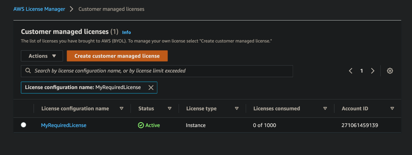
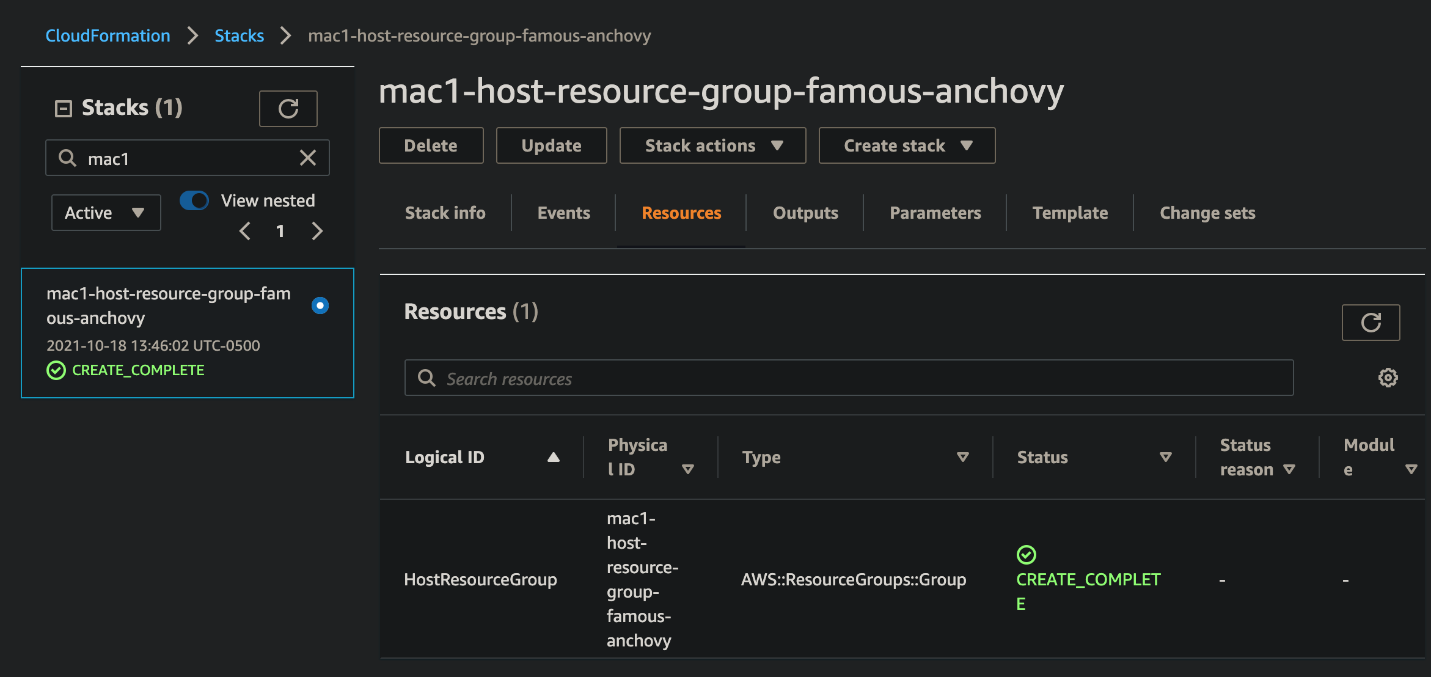
  2. Now that you’ve migrated your launch configurations to launch templates you can prevent users from creating new launch configurations by updating their IAM permissions to deny the autoscaling:CreateLaunchConfiguration action.

Instances launched by this Auto Scaling group continue to run and are not automatically be replaced by making this change. Any instance launched after making this change uses the launch template for its configuration. As your Auto Scaling group scales up and down, the older instances are replaced. If you’d like to force an update, you can use Instance Refresh to ensure that all instances are running the same launch template and version.
CloudFormation and Terraform

If you use CloudFormation to create and manage your infrastructure, you should use the AWS::EC2::LaunchTemplate resource to create launch templates. After adding a launch template resource to your CloudFormation stack template file update your Auto Scaling group resource definition by adding a LaunchTemplate property and removing the existing LaunchConfigurationName property. We have several examples available to help you get started.

Using launch templates with Terraform is a similar process. Update your template file to include a aws_launch_template resource and then update your aws_autoscaling_group resources to reference the launch template.

In addition to making these changes, you may also want to consider adding a MixedInstancesPolicy to your Auto Scaling group. A MixedInstancesPolicy allows you to configure your Auto Scaling group with multiple instance types and purchase options. This helps improve the availability and optimization of your applications. Some examples of these benefits include using Spot Instances and On-Demand Instances within the same Auto Scaling group, combining CPU architectures such as Intel, AMD, and ARM (Graviton2), and having multiple instance types configured in case of a temporary capacity issue.

You can generate and configure example templates for CloudFormation and Terraform in the AWS Management Console.

AWS CLI

If you’re using the AWS CLI to create and manage your Auto Scaling groups, these examples will show you how to accomplish common tasks when using launch templates.

SDKs

AWS SDKs already include APIs for creating launch templates. If you’re using one of our SDKs to create and configure your Auto Scaling groups, you can find more information in the SDK documentation for your language of choice.

Next steps

We’re excited to help you take advantage of the latest EC2 features by making the transition to launch templates as seamless as possible. As we make this transition together, we’re here to help and will continue to communicate our plans and timelines for this transition. If you are unable to transition to launch templates due to lack of tooling or functionalities or have any concerns, please contact AWS Support. Also, stay tuned for more information on tools to help make this transition easier for you.

AWS Lambda Functions Powered by AWS Graviton2 Processor – Run Your Functions on Arm and Get Up to 34% Better Price Performance

Post Syndicated from Danilo Poccia original https://aws.amazon.com/blogs/aws/aws-lambda-functions-powered-by-aws-graviton2-processor-run-your-functions-on-arm-and-get-up-to-34-better-price-performance/

Many of our customers (such as Formula One, Honeycomb, Intuit, SmugMug, and Snap Inc.) use the Arm-based AWS Graviton2 processor for their workloads and enjoy better price performance. Starting today, you can get the same benefits for your AWS Lambda functions. You can now configure new and existing functions to run on x86 or Arm/Graviton2 processors.

With this choice, you can save money in two ways. First, your functions run more efficiently due to the Graviton2 architecture. Second, you pay less for the time that they run. In fact, Lambda functions powered by Graviton2 are designed to deliver up to 19 percent better performance at 20 percent lower cost.

With Lambda, you are charged based on the number of requests for your functions and the duration (the time it takes for your code to execute) with millisecond granularity. For functions using the Arm/Graviton2 architecture, duration charges are 20 percent lower than the current pricing for x86. The same 20 percent reduction also applies to duration charges for functions using Provisioned Concurrency.

In addition to the price reduction, functions using the Arm architecture benefit from the performance and security built into the Graviton2 processor. Workloads using multithreading and multiprocessing, or performing many I/O operations, can experience lower execution time and, as a consequence, even lower costs. This is particularly useful now that you can use Lambda functions with up to 10 GB of memory and 6 vCPUs. For example, you can get better performance for web and mobile backends, microservices, and data processing systems.

If your functions don’t use architecture-specific binaries, including in their dependencies, you can switch from one architecture to the other. This is often the case for many functions using interpreted languages such as Node.js and Python or functions compiled to Java bytecode.

All Lambda runtimes built on top of Amazon Linux 2, including the custom runtime, are supported on Arm, with the exception of Node.js 10 that has reached end of support. If you have binaries in your function packages, you need to rebuild the function code for the architecture you want to use. Functions packaged as container images need to be built for the architecture (x86 or Arm) they are going to use.

To measure the difference between architectures, you can create two versions of a function, one for x86 and one for Arm. You can then send traffic to the function via an alias using weights to distribute traffic between the two versions. In Amazon CloudWatch, performance metrics are collected by function versions, and you can look at key indicators (such as duration) using statistics. You can then compare, for example, average and p99 duration between the two architectures.

You can also use function versions and weighted aliases to control the rollout in production. For example, you can deploy the new version to a small amount of invocations (such as 1 percent) and then increase up to 100 percent for a complete deployment. During rollout, you can lower the weight or set it to zero if your metrics show something suspicious (such as an increase in errors).

Let’s see how this new capability works in practice with a few examples.

Changing Architecture for Functions with No Binary Dependencies
When there are no binary dependencies, changing the architecture of a Lambda function is like flipping a switch. For example, some time ago, I built a quiz app with a Lambda function. With this app, you can ask and answer questions using a web API. I use an Amazon API Gateway HTTP API to trigger the function. Here’s the Node.js code including a few sample questions at the beginning:

const questions = [
  {
    question:
      "Are there more synapses (nerve connections) in your brain or stars in our galaxy?",
    answers: [
      "More stars in our galaxy.",
      "More synapses (nerve connections) in your brain.",
      "They are about the same.",
    ],
    correctAnswer: 1,
  },
  {
    question:
      "Did Cleopatra live closer in time to the launch of the iPhone or to the building of the Giza pyramids?",
    answers: [
      "To the launch of the iPhone.",
      "To the building of the Giza pyramids.",
      "Cleopatra lived right in between those events.",
    ],
    correctAnswer: 0,
  },
  {
    question:
      "Did mammoths still roam the earth while the pyramids were being built?",
    answers: [
      "No, they were all exctint long before.",
      "Mammooths exctinction is estimated right about that time.",
      "Yes, some still survived at the time.",
    ],
    correctAnswer: 2,
  },
];

exports.handler = async (event) => {
  console.log(event);

  const method = event.requestContext.http.method;
  const path = event.requestContext.http.path;
  const splitPath = path.replace(/^\/+|\/+$/g, "").split("/");

  console.log(method, path, splitPath);

  var response = {
    statusCode: 200,
    body: "",
  };

  if (splitPath[0] == "questions") {
    if (splitPath.length == 1) {
      console.log(Object.keys(questions));
      response.body = JSON.stringify(Object.keys(questions));
    } else {
      const questionId = splitPath[1];
      const question = questions[questionId];
      if (question === undefined) {
        response = {
          statusCode: 404,
          body: JSON.stringify({ message: "Question not found" }),
        };
      } else {
        if (splitPath.length == 2) {
          const publicQuestion = {
            question: question.question,
            answers: question.answers.slice(),
          };
          response.body = JSON.stringify(publicQuestion);
        } else {
          const answerId = splitPath[2];
          if (answerId == question.correctAnswer) {
            response.body = JSON.stringify({ correct: true });
          } else {
            response.body = JSON.stringify({ correct: false });
          }
        }
      }
    }
  }

  return response;
};

To start my quiz, I ask for the list of question IDs. To do so, I use curl with an HTTP GET on the /questions endpoint:

$ curl https://<api-id>.execute-api.us-east-1.amazonaws.com/questions
[
  "0",
  "1",
  "2"
]

Then, I ask more information on a question by adding the ID to the endpoint:

$ curl https://<api-id>.execute-api.us-east-1.amazonaws.com/questions/1
{
  "question": "Did Cleopatra live closer in time to the launch of the iPhone or to the building of the Giza pyramids?",
  "answers": [
    "To the launch of the iPhone.",
    "To the building of the Giza pyramids.",
    "Cleopatra lived right in between those events."
  ]
}

I plan to use this function in production. I expect many invocations and look for options to optimize my costs. In the Lambda console, I see that this function is using the x86_64 architecture.

Console screenshot.

Because this function is not using any binaries, I switch architecture to arm64 and benefit from the lower pricing.

Console screenshot.

The change in architecture doesn’t change the way the function is invoked or communicates its response back. This means that the integration with the API Gateway, as well as integrations with other applications or tools, are not affected by this change and continue to work as before.

I continue my quiz with no hint that the architecture used to run the code has changed in the backend. I answer back to the previous question by adding the number of the answer (starting from zero) to the question endpoint:

$ curl https://<api-id>.execute-api.us-east-1.amazonaws.com/questions/1/0
{
  "correct": true
}

That’s correct! Cleopatra lived closer in time to the launch of the iPhone than the building of the Giza pyramids. While I am digesting this piece of information, I realize that I completed the migration of the function to Arm and optimized my costs.

Changing Architecture for Functions Packaged Using Container Images
When we introduced the capability to package and deploy Lambda functions using container images, I did a demo with a Node.js function generating a PDF file with the PDFKit module. Let’s see how to migrate this function to Arm.

Each time it is invoked, the function creates a new PDF mail containing random data generated by the faker.js module. The output of the function is using the syntax of the Amazon API Gateway to return the PDF file using Base64 encoding. For convenience, I replicate the code (app.js) of the function here:

const PDFDocument = require('pdfkit');
const faker = require('faker');
const getStream = require('get-stream');

exports.lambdaHandler = async (event) => {

    const doc = new PDFDocument();

    const randomName = faker.name.findName();

    doc.text(randomName, { align: 'right' });
    doc.text(faker.address.streetAddress(), { align: 'right' });
    doc.text(faker.address.secondaryAddress(), { align: 'right' });
    doc.text(faker.address.zipCode() + ' ' + faker.address.city(), { align: 'right' });
    doc.moveDown();
    doc.text('Dear ' + randomName + ',');
    doc.moveDown();
    for(let i = 0; i < 3; i++) {
        doc.text(faker.lorem.paragraph());
        doc.moveDown();
    }
    doc.text(faker.name.findName(), { align: 'right' });
    doc.end();

    pdfBuffer = await getStream.buffer(doc);
    pdfBase64 = pdfBuffer.toString('base64');

    const response = {
        statusCode: 200,
        headers: {
            'Content-Length': Buffer.byteLength(pdfBase64),
            'Content-Type': 'application/pdf',
            'Content-disposition': 'attachment;filename=test.pdf'
        },
        isBase64Encoded: true,
        body: pdfBase64
    };
    return response;
};

To run this code, I need the pdfkit, faker, and get-stream npm modules. These packages and their versions are described in the package.json and package-lock.json files.

I update the FROM line in the Dockerfile to use an AWS base image for Lambda for the Arm architecture. Given the chance, I also update the image to use Node.js 14 (I was using Node.js 12 at the time). This is the only change I need to switch architecture.

FROM public.ecr.aws/lambda/nodejs:14-arm64
COPY app.js package*.json ./
RUN npm install
CMD [ "app.lambdaHandler" ]

For the next steps, I follow the post I mentioned previously. This time I use random-letter-arm for the name of the container image and for the name of the Lambda function. First, I build the image:

$ docker build -t random-letter-arm .

Then, I inspect the image to check that it is using the right architecture:

$ docker inspect random-letter-arm | grep Architecture

"Architecture": "arm64",

To be sure the function works with the new architecture, I run the container locally.

$ docker run -p 9000:8080 random-letter-arm:latest

Because the container image includes the Lambda Runtime Interface Emulator, I can test the function locally:

$ curl -XPOST "http://localhost:9000/2015-03-31/functions/function/invocations" -d '{}'

It works! The response is a JSON document containing a base64-encoded response for the API Gateway:

{
    "statusCode": 200,
    "headers": {
        "Content-Length": 2580,
        "Content-Type": "application/pdf",
        "Content-disposition": "attachment;filename=test.pdf"
    },
    "isBase64Encoded": true,
    "body": "..."
}

Confident that my Lambda function works with the arm64 architecture, I create a new Amazon Elastic Container Registry repository using the AWS Command Line Interface (CLI):

$ aws ecr create-repository --repository-name random-letter-arm --image-scanning-configuration scanOnPush=true

I tag the image and push it to the repo:

$ docker tag random-letter-arm:latest 123412341234.dkr.ecr.us-east-1.amazonaws.com/random-letter-arm:latest
$ aws ecr get-login-password | docker login --username AWS --password-stdin 123412341234.dkr.ecr.us-east-1.amazonaws.com
$ docker push 123412341234.dkr.ecr.us-east-1.amazonaws.com/random-letter-arm:latest

In the Lambda console, I create the random-letter-arm function and select the option to create the function from a container image.

Console screenshot.

I enter the function name, browse my ECR repositories to select the random-letter-arm container image, and choose the arm64 architecture.

Console screenshot.

I complete the creation of the function. Then, I add the API Gateway as a trigger. For simplicity, I leave the authentication of the API open.

Console screenshot.

Now, I click on the API endpoint a few times and download some PDF mails generated with random data:

Screenshot of some PDF files.

The migration of this Lambda function to Arm is complete. The process will differ if you have specific dependencies that do not support the target architecture. The ability to test your container image locally helps you find and fix issues early in the process.

Comparing Different Architectures with Function Versions and Aliases
To have a function that makes some meaningful use of the CPU, I use the following Python code. It computes all prime numbers up to a limit passed as a parameter. I am not using the best possible algorithm here, that would be the sieve of Eratosthenes, but it’s a good compromise for an efficient use of memory. To have more visibility, I add the architecture used by the function to the response of the function.

import json
import math
import platform
import timeit

def primes_up_to(n):
    primes = []
    for i in range(2, n+1):
        is_prime = True
        sqrt_i = math.isqrt(i)
        for p in primes:
            if p > sqrt_i:
                break
            if i % p == 0:
                is_prime = False
                break
        if is_prime:
            primes.append(i)
    return primes

def lambda_handler(event, context):
    start_time = timeit.default_timer()
    N = int(event['queryStringParameters']['max'])
    primes = primes_up_to(N)
    stop_time = timeit.default_timer()
    elapsed_time = stop_time - start_time

    response = {
        'machine': platform.machine(),
        'elapsed': elapsed_time,
        'message': 'There are {} prime numbers <= {}'.format(len(primes), N)
    }
    
    return {
        'statusCode': 200,
        'body': json.dumps(response)
    }

I create two function versions using different architectures.

Console screenshot.

I use a weighted alias with 50% weight on the x86 version and 50% weight on the Arm version to distribute invocations evenly. When invoking the function through this alias, the two versions running on the two different architectures are executed with the same probability.

Console screenshot.

I create an API Gateway trigger for the function alias and then generate some load using a few terminals on my laptop. Each invocation computes prime numbers up to one million. You can see in the output how two different architectures are used to run the function.

$ while True
  do
    curl https://<api-id>.execute-api.us-east-1.amazonaws.com/default/prime-numbers\?max\=1000000
  done

{"machine": "aarch64", "elapsed": 1.2595275060011772, "message": "There are 78498 prime numbers <= 1000000"}
{"machine": "aarch64", "elapsed": 1.2591725109996332, "message": "There are 78498 prime numbers <= 1000000"}
{"machine": "x86_64", "elapsed": 1.7200910530000328, "message": "There are 78498 prime numbers <= 1000000"}
{"machine": "x86_64", "elapsed": 1.6874686619994463, "message": "There are 78498 prime numbers <= 1000000"}
{"machine": "x86_64", "elapsed": 1.6865161940004327, "message": "There are 78498 prime numbers <= 1000000"}
{"machine": "aarch64", "elapsed": 1.2583248640003148, "message": "There are 78498 prime numbers <= 1000000"}
...

During these executions, Lambda sends metrics to CloudWatch and the function version (ExecutedVersion) is stored as one of the dimensions.

To better understand what is happening, I create a CloudWatch dashboard to monitor the p99 duration for the two architectures. In this way, I can compare the performance of the two environments for this function and make an informed decision on which architecture to use in production.

Console screenshot.

For this particular workload, functions are running much faster on the Graviton2 processor, providing a better user experience and much lower costs.

Comparing Different Architectures with Lambda Power Tuning
The AWS Lambda Power Tuning open-source project, created by my friend Alex Casalboni, runs your functions using different settings and suggests a configuration to minimize costs and/or maximize performance. The project has recently been updated to let you compare two results on the same chart. This comes in handy to compare two versions of the same function, one using x86 and the other Arm.

For example, this chart compares x86 and Arm/Graviton2 results for the function computing prime numbers I used earlier in the post:

Chart.

The function is using a single thread. In fact, the lowest duration for both architectures is reported when memory is configured with 1.8 GB. Above that, Lambda functions have access to more than 1 vCPU, but in this case, the function can’t use the additional power. For the same reason, costs are stable with memory up to 1.8 GB. With more memory, costs increase because there are no additional performance benefits for this workload.

I look at the chart and configure the function to use 1.8 GB of memory and the Arm architecture. The Graviton2 processor is clearly providing better performance and lower costs for this compute-intensive function.

Availability and Pricing
You can use Lambda Functions powered by Graviton2 processor today in US East (N. Virginia), US East (Ohio), US West (Oregon), Europe (Frankfurt), Europe (Ireland), EU (London), Asia Pacific (Mumbai), Asia Pacific (Singapore), Asia Pacific (Sydney), Asia Pacific (Tokyo).

The following runtimes running on top of Amazon Linux 2 are supported on Arm:

  • Node.js 12 and 14
  • Python 3.8 and 3.9
  • Java 8 (java8.al2) and 11
  • .NET Core 3.1
  • Ruby 2.7
  • Custom Runtime (provided.al2)

You can manage Lambda Functions powered by Graviton2 processor using AWS Serverless Application Model (SAM) and AWS Cloud Development Kit (AWS CDK). Support is also available through many AWS Lambda Partners such as AntStack, Check Point, Cloudwiry, Contino, Coralogix, Datadog, Lumigo, Pulumi, Slalom, Sumo Logic, Thundra, and Xerris.

Lambda functions using the Arm/Graviton2 architecture provide up to 34 percent price performance improvement. The 20 percent reduction in duration costs also applies when using Provisioned Concurrency. You can further reduce your costs by up to 17 percent with Compute Savings Plans. Lambda functions powered by Graviton2 are included in the AWS Free Tier up to the existing limits. For more information, see the AWS Lambda pricing page.

You can find help to optimize your workloads for the AWS Graviton2 processor in the Getting started with AWS Graviton repository.

Start running your Lambda functions on Arm today.

Danilo

Enabling parallel file systems in the cloud with Amazon EC2 (Part I: BeeGFS)

Post Syndicated from Ben Peven original https://aws.amazon.com/blogs/compute/enabling-parallel-file-systems-in-the-cloud-with-amazon-ec2-part-i-beegfs/

This post was authored by AWS Solutions Architects Ray Zaman, David Desroches, and Ameer Hakme.

In this blog series, you will discover how to build and manage your own Parallel Virtual File System (PVFS) on AWS. In this post you will learn how to deploy the popular open source parallel file system, BeeGFS, using AWS D3en and I3en EC2 instances. We will also provide a CloudFormation template to automate this BeeGFS deployment.

A PVFS is a type of distributed file system that distributes file data across multiple servers and provides concurrent data access to multiple execution tasks of an application. PVFS focuses on high-performance access to large datasets. It consists of a server process and a client library, which allows the file system to be mounted and used with standard utilities. PVFS on the Linux OS originated in the 1990’s and today several projects are available including Lustre, GlusterFS, and BeeGFS. Workloads such as shared storage for video transcoding and export, batch processing jobs, high frequency online transaction processing (OLTP) systems, and scratch storage for high performance computing (HPC) benefit from the high throughput and performance provided by PVFS.

Implementation of a PVFS can be complex and expensive. There are many variables you will want to take into account when designing a PVFS cluster including the number of nodes, node size (CPU, memory), cluster size, storage characteristics (size, performance), and network bandwidth. Due to the difficulty in estimating the correct configuration, systems procured for on-premises data centers are typically oversized, resulting in additional costs, and underutilized resources. In addition, the hardware procurement process is lengthy and the installation and maintenance of the hardware adds additional overhead.

AWS makes it easy to run and fully manage your parallel file systems by allowing you to choose from a variety of Amazon Elastic Compute Cloud (EC2) instances. EC2 instances are available on-demand and allow you to scale your workload as needed. AWS storage-optimized EC2 instances offer up to 60 TB of NVMe SSD storage per instance and up to 336 TB of local HDD storage per instance. With storage-optimized instances, you can easily deploy PVFS to support workloads requiring high-performance access to large datasets. You can test and iterate on different instances to find the optimal size for your workloads.

D3en instances leverage 2nd-generation Intel Xeon Scalable Processors (Cascade Lake) and provide a sustained all core frequency up to 3.1 GHz. These instances provide up to 336 TB of local HDD storage (which is the highest local storage capacity in EC2), up to 6.2 GiBps of disk throughput, and up to 75 Gbps of network bandwidth.

I3en instances are powered by 1st or 2nd generation Intel® Xeon® Scalable (Skylake or Cascade Lake) processors with 3.1 GHz sustained all-core turbo performance. These instances provide up to 60 TB of NVMe storage, up to 16 GB/s of sequential disk throughput, and up to 100 Gbps of network bandwidth.

BeeGFS, originally released by ThinkParQ in 2014, is an open source, software defined PVFS that runs on Linux. You can scale the size and performance of the BeeGFS file-system by configuring the number of servers and disks in the clusters up to thousands of nodes.

BeeGFS architecture

D3en instances offer HDD storage while I3en instances offer NVMe SSD storage. This diversity allows you to create tiers of storage based on performance requirements. In the example presented in this post you will use four D3en.8xlarge (32 vCPU, 128 GB, 16x14TB HDD, 50 Gbit) and two I3en.12xlarge (48 vCPU, 384 GB, 4 x 7.5-TB NVMe) instances to create two storage tiers. You may choose different sizes and quantities to meet your needs. The I3en instances, with SSD, will be configured as tier 1 and the D3en instances, with HDD, will be configured as tier 2. One disk from each instance will be formatted as ext4 and used for metadata while the remaining disks will be formatted as XFS and used for storage. You may choose to separate metadata and storage on different hosts for workloads where these must scale independently. The array will be configured RAID 0, since it will provide maximum performance. Software replication or other RAID types can be employed for higher durability.

BeeGFS architecture

Figure 1: BeeGFS architecture

You will deploy all instances within a single VPC in the same Availability Zone and subnet to minimize latency. Security groups must be configured to allow the following ports:

  • Management service (beegfs-mgmtd): 8008
  • Metadata service (beegfs-meta): 8005
  • Storage service (beegfs-storage): 8003
  • Client service (beegfs-client): 8004

You will use the Debian Quick Start Amazon Machine Image (AMI) as it supports BeeGFS. You can enable Amazon CloudWatch to capture metrics.

How to deploy the BeeGFS architecture

Follow the steps below to create the PVFS described above. For automated deployment, use the CloudFormation template located at AWS Samples.

  1. Use the AWS Management Console or CLI to deploy one D3en.8xlarge instance into a VPC as described above.
  2. Log in to the instance and update the system:
    • sudo apt update
    • sudo apt upgrade
  3. Install the XFS utilities and load the kernel module:
    • sudo apt-get -y install xfsprogs
    • sudo modprobe -v xfs

Format the first disk ext4 as it is used for metadata, the rest are formatted xfs. The disks will appear as “nvme???” which actually represent the HDD drives on the D3en instances.

4. View a listing of available disks:

    • sudo lsblk

5. Format hard disks:

    • sudo mkfs -t ext4 /dev/nvme0n1
    • sudo mkfs -t xfs /dev/nvme1n1
    • Repeat this command for disks nvme2n1 through nvme15n1

6. Create file system mount points:

    • sudo mkdir /disk00
    • sudo mkdir /disk01
    • Repeat this command for disks disk02 through disk15

7. Mount the filesystems:

    • sudo mount /dev/nvme0n1 /disk00
    • sudo mount /dev/nvme0n1 /disk01
    • Repeat this command for disks disk02 through disk15

Repeat steps 1 through 7 on the remaining nodes. Remember to account for fewer disks for i3en.12xlarge instances or if you decide to use different instance sizes.

8. Add the BeeGFS Repo to each node:

    • sudo apt-get -y install gnupg
    • wget https://www.beegfs.io/release/beegfs_7.2.3/dists/beegfs-deb10.list
    • sudo cp beegfs-deb10.list /etc/apt/sources.list.d/
    • sudo wget -q https://www.beegfs.io/release/latest-stable/gpg/DEB-GPG-KEY-beegfs -O- | sudo apt-key add -
    • sudo apt update

9. Install BeeGFS management (node 1 only):

    • sudo apt-get -y install beegfs-mgmtd
    • sudo mkdir /beegfs-mgmt
    • sudo /opt/beegfs/sbin/beegfs-setup-mgmtd -p /beegfs-mgmt/beegfs/beegfs_mgmtd

10. Install BeeGFS metadata and storage (all nodes):

    • sudo apt-get -y install beegfs-meta beegfs-storage beegfs-meta beegfs-client beegfs-helperd beegfs-utils
    • # -s is unique ID based on node - change this!, -m is hostname of management server
    • sudo /opt/beegfs/sbin/beegfs-setup-meta -p /disk00/beegfs/beegfs_meta -s 1 -m ip-XXX-XXX-XXX-XXX
    • # Change -s to nodeID and -i to (nodeid)0(disk), -m is hostname of management server
    • sudo /opt/beegfs/sbin/beegfs-setup-storage -p /disk01/beegfs_storage -s 1 -i 101 -m ip-XXX-XXX-XXX-XXX
    • sudo /opt/beegfs/sbin/beegfs-setup-storage -p /disk02/beegfs_storage -s 1 -i 102 -m ip-XXX-XXX-XXX-XXX
    • Repeat this last command for the remaining disks disk03 through disk15

11. Start the services:

    • #Only on node1
    • sudo systemctl start beegfs-mgmtd
    • #All servers
    • sudo systemctl start beegfs-meta
    • sudo systemctl start beegfs-storage

At this point, your BeeGFS cluster is running and ready for use by a client system. The client system requires BeeGFS client software in order to mount the cluster.

12. Deploy an m5n.2xlarge instance into the same subnet as the PVFS cluster.

13. Log in to the instance, install, and configure the client:

    • sudo apt update
    • sudo apt upgrade
    • sudo apt-get -y install gnupg
    • #Need linux sources for client compilation
    • sudo apt-get -y install linux-source
    • sudo apt-get -y install linux-headers-4.19.0-14-all
    • wget https://www.beegfs.io/release/beegfs_7.2.3/dists/beegfs-deb10.list
    • sudo cp beegfs-deb10.list /etc/apt/sources.list.d/
    • sudo wget -q https://www.beegfs.io/release/latest-stable/gpg/DEB-GPG-KEY-beegfs -O- | sudo apt-key add -
    • sudo apt update
    • sudo apt-get -y install beegfs-client beegfs-helperd beegfs-utils
    • sudo /opt/beegfs/sbin/beegfs-setup-client -m ip-XXX-XXX-XXX-XX # use the ip address of the management node
    • sudo systemctl start beegfs-helperd
    • sudo systemctl start beegfs-client

14. Create the storage pools:

    • sudo beegfs-ctl --addstoragepool —desc="tier1" —targets=501,502,503,601,602,603
    • sudo beegfs-ctl --addstoragepool --desc="tier2" --targets=101,102,103,104,105,106,107,108,109,110,111,112,113,114,115,201,202,203,204,205,206,207,208,209,210,
      211,212,213,214,215,301,302,303,304,305,306,307,308,309,310,311,312,313,314,315,401,402,403,404,405,406,407,
      408,409,410,411,412,413,414,415
    • sudo beegfs-ctl --liststoragepools
    • Pool ID Pool Description                      Targets                 Buddy Groups
    • ======= ================== ============================ ============================
      • Default
      • tier1 501,502,503,601,602,603
      • tier2 101,102,103,104,105,106,107,
        • 108,109,110,111,112,113,114,
        • 115,201,202,203,204,205,206,
        • 207,208,209,210,211,212,213,
        • 214,215,301,302,303,304,305,
        • 306,307,308,309,310,311,312,
        • 313,314,315,401,402,403,404,
        • 405,406,407,408,409,410,411,
        • 412,413,414,415

15. Mount the pools to the file system:

    • sudo beegfs-ctl --setpattern --storagepoolid=2 /mnt/beegfs/tier1
    • sudo beegfs-ctl --setpattern --storagepoolid=3 /mnt/beegfs/tier2

The BeeGFS PVFS is now ready to be used by the client system.

How to test your new BeeGFS PVFS

BeeGFS provides StorageBench to evaluate the performance of BeeGFS on the storage targets. This benchmark measures the streaming throughput of the underlying file system and devices independent of the network performance. To simulate client I/O, this benchmark generates read/write locally on the servers without any client communication.

It is possible to benchmark specific targets or all targets together using the “servers” parameter. A “read” or “write” parameter sets the type pf test to perform. The “threads” parameter is set to the number of storage devices.

Try the following commands to test performance:

Write test (1x d3en):

sudo beegfs-ctl --storagebench --servers=1 --write --blocksize=512K —size=20G —threads=15

Write test (4x d3en):

sudo beegfs-ctl --storagebench --alltargets --write --blocksize=512K —size=20G —threads=15

Read test (4x d3en):

sudo beegfs-ctl --storagebench --servers=1,2,3,4 --read --blocksize=512K --size=20G --threads=15

Write test (1x i3en):

sudo beegfs-ctl --storagebench --servers=5 --write --blocksize=512K --size=20G --threads=3

Read test (2x i3en):

sudo beegfs-ctl --storagebench --servers=5,6 --read --blocksize=512K —size=20G —threads=3

StorageBench is a great way to test what the potential performance of a given environment looks like by reducing variables like network throughput and latency, but you may want to test in a more real-world fashion. For this, tools like ‘fio’ can generate mixed read/write workloads against files on the client BeeGFS mountpoint.

First, we need to define which directory goes to which Storage Pool (tier) by setting a pattern:

sudo beegfs-ctl --setpattern --storagepoolid=2 /mnt/beegfs/tier1 sudo beegfs-ctl --setpattern --storagepoolid=3 /mnt/beegfs/tier2

You can see how a file gets striped across the various disks in a pool by adding a file and running the command:

sudo beegfs-ctl —getentryinfo /mnt/beegfs/tier1/myfile.bin

Install fio:

sudo apt-get install -y fio

Now you can run a fio test against one of the tiers.  This example command runs eight threads running a 75/25 read/write workload against a 10-GB file:

sudo fio --numjobs=8 --randrepeat=1 --ioengine=libaio --direct=1 --gtod_reduce=1 --name=test --filename=/mnt/beegfs/tier1/test --bs=512k --iodepth=64 --size=10G --readwrite=randrw --rwmixread=75

Cleaning up

To avoid ongoing charges for resources you created, you should:

Conclusion

In this blog post we demonstrated how to build and manage your own BeeGFS Parallel Virtual File System on AWS. In this example, you created two storage tiers using the I3en and D3en. The I3en was used as the first tier for SSD storage and the D3en was used as a second tier for HDD storage. By using two different tiers, you can optimize performance to meet your application requirements.

Amazon EC2 storage-optimized instances make it easy to deploy the BeeGFS Parallel Virtual File System. Using combinations of SSD and HDD storage available on the I3en and D3en instance types, you can achieve the capacity and performance needed to run the most demanding workloads. Read more about the D3en and I3en instances.

Use Amazon ECS Fargate Spot with CircleCI to deploy and manage applications in a cost-effective way

Post Syndicated from Pritam Pal original https://aws.amazon.com/blogs/devops/deploy-apps-cost-effective-way-with-ecs-fargate-spot-and-circleci/

This post is written by Pritam Pal, Sr EC2 Spot Specialist SA & Dan Kelly, Sr EC2 Spot GTM Specialist

Customers are using Amazon Web Services (AWS) to build CI/CD pipelines and follow DevOps best practices in order to deliver products rapidly and reliably. AWS services simplify infrastructure provisioning and management, application code deployment, software release processes automation, and application and infrastructure performance monitoring. Builders are taking advantage of low-cost, scalable compute with Amazon EC2 Spot Instances, as well as AWS Fargate Spot to build, deploy, and manage microservices or container-based workloads at a discounted price.

Amazon EC2 Spot Instances let you take advantage of unused Amazon Elastic Compute Cloud (Amazon EC2) capacity at steep discounts as compared to on-demand pricing. Fargate Spot is an AWS Fargate capability that can run interruption-tolerant Amazon Elastic Container Service (Amazon ECS) tasks at up to a 70% discount off the Fargate price. Since tasks can still be interrupted, only fault tolerant applications are suitable for Fargate Spot. However, for flexible workloads that can be interrupted, this feature enables significant cost savings over on-demand pricing.

CircleCI provides continuous integration and delivery for any platform, as well as your own infrastructure. CircleCI can automatically trigger low-cost, serverless tasks with AWS Fargate Spot in Amazon ECS. Moreover, CircleCI Orbs are reusable packages of CircleCI configuration that help automate repeated processes, accelerate project setup, and ease third-party tool integration. Currently, over 1,100 organizations are utilizing the CircleCI Amazon ECS Orb to power/run 250,000+ jobs per month.

Customers are utilizing Fargate Spot for a wide variety of workloads, such as Monte Carlo simulations and genomic processing. In this blog, I utilize a python code with the Tensorflow library that can run as a container image in order to train a simple linear model. It runs the training steps in a loop on a data batch and periodically writes checkpoints to S3. If there is a Fargate Spot interruption, then it restores the checkpoint from S3 (when a new Fargate Instance occurs) and continues training. We will deploy this on AWS ECS Fargate Spot for low-cost, serverless task deployment utilizing CircleCI.

Concepts

Before looking at the solution, let’s revisit some of the concepts we’ll be using.

Capacity Providers: Capacity providers let you manage computing capacity for Amazon ECS containers. This allows the application to define its requirements for how it utilizes the capacity. With capacity providers, you can define flexible rules for how containerized workloads run on different compute capacity types and manage the capacity scaling. Furthermore, capacity providers improve the availability, scalability, and cost of running tasks and services on Amazon ECS. In order to run tasks, the default capacity provider strategy will be utilized, or an alternative strategy can be specified if required.

AWS Fargate and AWS Fargate Spot capacity providers don’t need to be created. They are available to all accounts and only need to be associated with a cluster for utilization. When a new cluster is created via the Amazon ECS console, along with the Networking-only cluster template, the FARGATE and FARGATE_SPOT capacity providers are automatically associated with the new cluster.

CircleCI Orbs: Orbs are reusable CircleCI configuration packages that help automate repeated processes, accelerate project setup, and ease third-party tool integration. Orbs can be found in the developer hub on the CircleCI orb registry. Each orb listing has usage examples that can be referenced. Moreover, each orb includes a library of documented components that can be utilized within your config for more advanced purposes. Since the 2.0.0 release, the AWS ECS Orb supports the capacity provider strategy parameter for running tasks allowing you to efficiently run any ECS task against your new or existing clusters via Fargate Spot capacity providers.

Solution overview

Fargate Spot helps cost-optimize services that can handle interruptions like Containerized workloads, CI/CD, or Web services behind a load balancer. When Fargate Spot needs to interrupt a running task, it sends a SIGTERM signal. It is best practice to build applications capable of responding to the signal and shut down gracefully.

This walkthrough will utilize a capacity provider strategy leveraging Fargate and Fargate Spot, which mitigates risk if multiple Fargate Spot tasks get terminated simultaneously. If you’re unfamiliar with Fargate Spot, capacity providers, or capacity provider strategies, read our previous blog about Fargate Spot best practices here.

Prerequisites

Our walkthrough will utilize the following services:

  • GitHub as a code repository
  • AWS Fargate/Fargate Spot for running your containers as ECS tasks
  • CircleCI for demonstrating a CI/CD pipeline. We will utilize CircleCI Cloud Free version, which allows 2,500 free credits/week and can run 1 job at a time.

We will run a Job with CircleCI ECS Orb in order to deploy 4 ECS Tasks on Fargate and Fargate Spot. You should have the following prerequisites:

  1. An AWS account
  2. A GitHub account

Walkthrough

Step 1: Create AWS Keys for Circle CI to utilize.

Head to AWS IAM console, create a new user, i.e., circleci, and select only the Programmatic access checkbox. On the set permission page, select Attach existing policies directly. For the sake of simplicity, we added a managed policy AmazonECS_FullAccess to this user. However, for production workloads, employ a further least-privilege access model. Download the access key file, which will be utilized to connect to CircleCI in the next steps.

Step 2: Create an ECS Cluster, Task definition, and ECS Service

2.1 Open the Amazon ECS console

2.2 From the navigation bar, select the Region to use

2.3 In the navigation pane, choose Clusters

2.4 On the Clusters page, choose Create Cluster

2.5 Create a Networking only Cluster ( Powered by AWS Fargate)

Amazon ECS Create Cluster

This option lets you launch a cluster in your existing VPC to utilize for Fargate tasks. The FARGATE and FARGATE_SPOT capacity providers are automatically associated with the cluster.

2.6 Click on Update Cluster to define a default capacity provider strategy for the cluster, then add FARGATE and FARGATE_SPOT capacity providers each with a weight of 1. This ensures Tasks are divided equally among Capacity providers. Define other ratios for splitting your tasks between Fargate and Fargate Spot tasks, i.e., 1:1, 1:2, or 3:1.

ECS Update Cluster Capacity Providers

2.7 Here we will create a Task Definition by using the Fargate launch type, give it a name, and specify the task Memory and CPU needed to run the task. Feel free to utilize any Fargate task definition. You can use your own code, add the code in a container, or host the container in Docker hub or Amazon ECR. Provide a name and image URI that we copied in the previous step and specify the port mappings. Click Add and then click Create.

We are also showing an example of a python code using the Tensorflow library that can run as a container image in order to train a simple linear model. It runs the training steps in a loop on a batch of data, and it periodically writes checkpoints to S3. Please find the complete code here. Utilize a Dockerfile to create a container from the code.

Sample Docker file to create a container image from the code mentioned above.

FROM ubuntu:18.04
WORKDIR /app
COPY . /app
RUN pip install -r requirements.txt EXPOSE 5000 CMD python tensorflow_checkpoint.py

Below is the Code Snippet we are using for Tensorflow to Train and Checkpoint a Training Job.


def train_and_checkpoint(net, manager):
  ckpt.restore(manager.latest_checkpoint).expect_partial()
  if manager.latest_checkpoint:
    print("Restored from {}".format(manager.latest_checkpoint))
  else:
    print("Initializing from scratch.")
  for _ in range(5000):
    example = next(iterator)
    loss = train_step(net, example, opt)
    ckpt.step.assign_add(1)
    if int(ckpt.step) % 10 == 0:
        save_path = manager.save()
        list_of_files = glob.glob('tf_ckpts/*.index')
        latest_file = max(list_of_files, key=os.path.getctime)
        upload_file(latest_file, 'pythontfckpt', object_name=None)
        list_of_files = glob.glob('tf_ckpts/*.data*')
        latest_file = max(list_of_files, key=os.path.getctime)
        upload_file(latest_file, 'pythontfckpt', object_name=None)
        upload_file('tf_ckpts/checkpoint', 'pythontfckpt', object_name=None)

2.8 Next, we will create an ECS Service, which will be used to fetch Cluster information while running the job from CircleCI. In the ECS console, navigate to your Cluster, From Services tab, then click create. Create an ECS service by choosing Cluster default strategy from the Capacity provider strategy dropdown. For the Task Definition field, choose webapp-fargate-task, which is the one we created earlier, enter a service name, set the number of tasks to zero at this point, and then leave everything else as default. Click Next step, select an existing VPC and two or more Subnets, keep everything else default, and create the service.

Step 3: GitHub and CircleCI Configuration

Create a GitHub repository, i.e., circleci-fargate-spot, and then create a .circleci folder and a config file config.yml. If you’re unfamiliar with GitHub or adding a repository, check the user guide here.

For this project, the config.yml file contains the following lines of code that configure and run your deployments.

version: '2.1'
orbs:
  aws-ecs: circleci/[email protected]
  aws-cli: circleci/[email protected]
  orb-tools: circleci/[email protected]
  shellcheck: circleci/[email protected]
  jq: circleci/[email protected]

jobs:  

  test-fargatespot:
      docker:
        - image: cimg/base:stable
      steps:
        - aws-cli/setup
        - jq/install
        - run:
            name: Get cluster info
            command: |
              SERVICES_OBJ=$(aws ecs describe-services --cluster "${ECS_CLUSTER_NAME}" --services "${ECS_SERVICE_NAME}")
              VPC_CONF_OBJ=$(echo $SERVICES_OBJ | jq '.services[].networkConfiguration.awsvpcConfiguration')
              SUBNET_ONE=$(echo "$VPC_CONF_OBJ" |  jq '.subnets[0]')
              SUBNET_TWO=$(echo "$VPC_CONF_OBJ" |  jq '.subnets[1]')
              SECURITY_GROUP_IDS=$(echo "$VPC_CONF_OBJ" |  jq '.securityGroups[0]')
              CLUSTER_NAME=$(echo "$SERVICES_OBJ" |  jq '.services[].clusterArn')
              echo "export SUBNET_ONE=$SUBNET_ONE" >> $BASH_ENV
              echo "export SUBNET_TWO=$SUBNET_TWO" >> $BASH_ENV
              echo "export SECURITY_GROUP_IDS=$SECURITY_GROUP_IDS" >> $BASH_ENV=$SECURITY_GROUP_IDS=$SECURITY_GROUP_IDS" >> $BASH_ENV" >> $BASH_ENV
              echo "export CLUSTER_NAME=$CLUSTER_NAME" >> $BASH_ENV
        - run:
            name: Associate cluster
            command: |
              aws ecs put-cluster-capacity-providers \
                --cluster "${ECS_CLUSTER_NAME}" \
                --capacity-providers FARGATE FARGATE_SPOT  \
                --default-capacity-provider-strategy capacityProvider=FARGATE,weight=1 capacityProvider=FARGATE_SPOT,weight=1\                --region ${AWS_DEFAULT_REGION}
        - aws-ecs/run-task:
              cluster: $CLUSTER_NAME
              capacity-provider-strategy: capacityProvider=FARGATE,weight=1 capacityProvider=FARGATE_SPOT,weight=1
              launch-type: ""
              task-definition: webapp-fargate-task
              subnet-ids: '$SUBNET_ONE, $SUBNET_TWO'
              security-group-ids: $SECURITY_GROUP_IDS
              assign-public-ip : ENABLED
              count: 4

workflows:
  run-task:
    jobs:
      - test-fargatespot

Now, Create a CircleCI account. Choose Login with GitHub. Once you’re logged in from the CircleCI dashboard, click Add Project and add the project circleci-fargate-spot from the list shown.

When working with CircleCI Orbs, you will need the config.yml file and environment variables under Project Settings.

The config file utilizes CircleCI version 2.1 and various Orbs, i.e., AWS-ECS, AWS-CLI, and JQ.  We will use a job test-fargatespot, which uses a Docker image, and we will setup the environment. In config.yml we are using the jq tool to parse JSON and fetch the ECS cluster information like VPC config, Subnets, and Security Groups needed to run an ECS task. As we are utilizing the capacity-provider-strategy, we will set the launch type parameter to an empty string.

In order to run a task, we will demonstrate how to override the default Capacity Provider strategy with Fargate & Fargate Spot, both with a weight of 1, and to divide tasks equally among Fargate & Fargate Spot. In our example, we are running 4 tasks, so 2 should run on Fargate and 2 on Fargate Spot.

Parameters like ECS_SERVICE_NAME, ECS_CLUSTER_NAME and other AWS access specific details are added securely under Project Settings and can be utilized by other jobs running within the project.

Add the following environment variables under Project Settings

    • AWS_ACCESS_KEY_ID – From Step 1
    • AWS_SECRET_ACCESS_KEY – From Step 1
    • AWS_DEFAULT_REGION – i.e. : – us-west-2
    • ECS_CLUSTER_NAME – From Step 2
    • ECS_SERVICE_NAME – From Step 2
    • SECURITY_GROUP_IDS – Security Group that will be used to run the task

Circle CI Environment Variables


Step 4: Run Job

Now in the CircleCI console, navigate to your project, choose the branch, and click Edit Config to verify that config.xml is correctly populated. Check for the ribbon at the bottom. A green ribbon means that the config file is valid and ready to run. Click Commit & Run from the top-right menu.

Click build Status to check its progress as it runs.

CircleCI Project Dashboard


A successful build should look like the one below. Expand each section to see the output.


CircleCI Job Configuration

Return to the ECS console, go to the Tasks Tab, and check that 4 new tasks are running. Click each task for the Capacity provider details. Two tasks should have run with FARGATE_SPOT as a Capacity provider, and two should have run with FARGATE.

Congratulations!

You have successfully deployed ECS tasks utilizing CircleCI on AWS Fargate and Fargate Spot. If you have used any sample web applications, then please use the public IP address to see the page. If you have used the sample code that we provided, then you should see Tensorflow training jobs running on Fargate instances. If there is a Fargate Spot interruption, then it restores the checkpoint from S3 when a new Fargate Instance comes up and continues training.

Cleaning up

In order to avoid incurring future charges, delete the resources utilized in the walkthrough. Go to the ECS console and Task tab.

  • Delete any running Tasks.
  • Delete ECS cluster.
  • Delete the circleci user from IAM console.

Cost analysis in Cost Explorer

In order to demonstrate a cost breakdown between the tasks running on Fargate and Fargate Spot, we left the tasks running for a day. Then, we utilized Cost Explorer with the following filters and groups in order discover the savings by running Fargate Spot.

Apply a filter on Service for ECS on the right-side filter, set Group by to Usage Type, and change the time period to the specific day.

Cost analysis in Cost Explorer

The cost breakdown demonstrates how Fargate Spot usage (indicated by “SpotUsage”) was significantly less expensive than non-Spot Fargate usage. Current Fargate Spot Pricing can be found here.

Conclusion

In this blog post, we have demonstrated how to utilize CircleCI to deploy and manage ECS tasks and run applications in a cost-effective serverless approach by using Fargate Spot.

Author bio

Pritam is a Sr. Specialist Solutions Architect on the EC2 Spot team. For the last 15 years, he evangelized DevOps and Cloud adoption across industries and verticals. He likes to deep dive and find solutions to everyday problems.
Dan is a Sr. Spot GTM Specialist on the EC2 Spot Team. He works closely with Amazon Partners to ensure that their customers can optimize and modernize their compute with EC2 Spot.


Improve the performance of Lambda applications with Amazon CodeGuru Profiler

Post Syndicated from Vishaal Thanawala original https://aws.amazon.com/blogs/devops/improve-performance-of-lambda-applications-amazon-codeguru-profiler/

As businesses expand applications to reach more users and devices, they risk higher latencies that could degrade the  customer experience. Slow applications can frustrate or even turn away customers. Developers therefore increasingly face the challenge of ensuring that their code runs as efficiently as possible, since application performance can make or break businesses.

Amazon CodeGuru Profiler helps developers improve their application speed by analyzing its runtime. CodeGuru Profiler analyzes single and multi-threaded applications and then generates visualizations to help developers understand the latency sources. Afterwards, CodeGuru Profiler provides recommendations to help resolve the root cause.

CodeGuru Profiler recently began providing recommendations for applications written in Python. Additionally, the new automated onboarding process for AWS Lambda functions makes it even easier to use CodeGuru Profiler with serverless applications built on AWS Lambda.

This post highlights these new features by explaining how to set up and utilize CodeGuru Profiler on an AWS Lambda function written in Python.

Prerequisites

This post focuses on improving the performance of an application written with AWS Lambda, so it’s important to understand the Lambda functions that work best with CodeGuru Profiler. You will get the most out of CodeGuru Profiler on long-duration Lambda functions (>10 seconds) or frequently invoked shorter generation Lambda functions (~100 milliseconds). Because CodeGuru Profiler requires five minutes of runtime data before the Lambda container is recycled, very short duration Lambda functions with an execution time of 1-10 milliseconds may not provide sufficient data for CodeGuru Profiler to generate meaningful results.

The automated CodeGuru Profiler onboarding process, which automatically creates the profiling group for you, supports Lambda functions running on Java 8 (Amazon Corretto), Java 11, and Python 3.8 runtimes. Additional runtimes, without the automated onboarding process, are supported and can be found in the Java documentation and the Python documentation.

Getting Started

Let’s quickly demonstrate the new Lambda onboarding process and the new Python recommendations. This example assumes you have already created a Lambda function, so we will just walk through the process of turning on CodeGuru Profiler and viewing results. If you don’t already have a Lambda function created, you can create one by following these set up instructions. If you would like to replicate this example, the code we used can be found on GitHub here.

  1. On the AWS Lambda Console page, open your Lambda function. For this example, we’re using a function with a Python 3.8 runtime.

 This image shows the Lambda console page for the Lambda function we are referencing.

2. Navigate to the Configuration tab, go to the Monitoring and operations tools page, and click Edit on the right side of the page.

This image shows the instructions to open the page to turn on profiling

3. Scroll down to “Amazon CodeGuru Profiler” and click the button next to “Code profiling” to turn it on. After enabling Code profiling, click Save.

This image shows how to turn on CodeGuru Profiler

4. Verify that CodeGuru Profiler has been turned on within the Monitoring and operations tools page

This image shows how to validate Code profiling has been turned on

That’s it! You can now navigate to CodeGuru Profiler within the AWS console and begin viewing results.

Viewing your results

CodeGuru Profiler requires 5 minutes of Lambda runtime data to generate results. After your Lambda function provides this runtime data, which may need multiple runs if your lambda has a short runtime, it will display within the “Profiling group” page in the CodeGuru Profiler console. The profiling group will be given a default name (i.e., aws-lambda-<lambda-function-name>), and it will take approximately 15 minutes after CodeGuru Profiler receives the runtime data before it appears on this page.

This image shows where you can see the profiling group created after turning on CodeGuru Profiler on your Lambda function

After the profile appears, customers can view their profiling results by analyzing the flame graphs. Additionally, after approximately 1 hour, customers will receive their first recommendation set (if applicable). For more information on how to reading the CodeGuru Profiler results, see Investigating performance issues with Amazon CodeGuru Profiler.

The below images show the two flame graphs (CPU Utilization and Latency) generated from profiling the Lambda function. Note that the highlighted horizontal bar (also referred to as a frame) in both images corresponds with one of the three frames that generates a recommendation. We’ll dive into more details on the recommendation in the following sections.

CPU Utilization Flame Graph:

This image shows the CPU Utilization flame graph for the Lambda function

Latency Flame Graph:

This image shows the Latency flame graph for the Lambda function

Here are the three recommendations generated from the above Lambda function:

This image shows the 3 recommendations generated by CodeGuru Profiler

Addressing a recommendation

Let’s dive even further into it an example recommendation. The first recommendation above notices that the Lambda function is spending more than the normal amount of runnable time (6.8% vs <1%) creating AWS SDK service clients. It recommends ensuring that the function doesn’t unnecessarily create AWS SDK service clients, which wastes CPU time.

This image shows the detailed recommendation for 'Recreation of AWS SDK service clients'

Based on the suggested resolution step, we made a quick and easy code change, moving the client creation outside of the lambda-handler function. This ensures that we don’t create unnecessary AWS SDK clients. The code change below shows how we would resolve the issue.

...
s3_client = boto3.client('s3')
cw_client = boto3.client('cloudwatch')

def lambda_handler(event, context):
...

Reviewing your savings

After making each of the three changes recommended above by CodeGuru Profiler, look at the new flame graphs to see how the changes impacted the applications profile. You’ll notice below that we no longer see the previously wide frames for boto3 clients, put_metric_data, or the logger in the S3 API call.

CPU Utilization Flame Graph:

This image shows the CPU Utilization flame graph after making the recommended changes

Latency Flame Graph:

This image shows the Latency flame graph after making the recommended changes

Moreover, we can run the Lambda function for one day (1439 invocations) and see the results in Lambda Insights in order to understand our total savings. After every recommendation was addressed, this Lambda function, with a 128 MB memory and 10 second timeout, decreased in CPU time by 10% and dropped in maximum memory usage and network IO leading to a 30% drop in GB-s. Decreasing GB-s leads to 30% lower cost for the Lambda’s duration bill as explained in the AWS Lambda Pricing.

Latency (before and after CodeGuru Profiler):

The graph below displays the duration change while running the Lambda function for 1 day.

This image shows the duration change while running the Lambda function for 1 day.

Cost (before and after CodeGuru Profiler):

The graph below displays the function cost change while running the lambda function for 1 day.

This image shows the function cost change while running the lambda function for 1 day.

Conclusion

This post showed how developers can easily onboard onto CodeGuru Profiler in order to improve the performance of their serverless applications built on AWS Lambda. Get started with CodeGuru Profiler by visiting the CodeGuru console.

All across Amazon, numerous teams have utilized CodeGuru Profiler’s technology to generate performance optimizations for customers. It has also reduced infrastructure costs, saving millions of dollars annually.

Onboard your Python applications onto CodeGuru Profiler by following the instructions on the documentation. If you’re interested in the Python agent, note that it is open-sourced on GitHub. Also for more demo applications using the Python agent, check out the GitHub repository for additional samples.

About the authors

Headshot of Vishaal

Vishaal is a Product Manager at Amazon Web Services. He enjoys getting to know his customers’ pain points and transforming them into innovative product solutions.


Headshot of Mirela

Mirela is working as a Software Development Engineer at Amazon Web Services as part of the CodeGuru Profiler team in London. Previously, she has worked for Amazon.com’s teams and enjoys working on products that help customers improve their code and infrastructure.


Headshot of Parag

Parag is a Software Development Engineer at Amazon Web Services as part of the CodeGuru Profiler team in Seattle. Previously, he was working for Amazon.com’s catalog and selection team. He enjoys working on large scale distributed systems and products that help customers build scalable, and cost-effective applications.

Run a Spark SQL-based ETL pipeline with Amazon EMR on Amazon EKS

Post Syndicated from Melody Yang original https://aws.amazon.com/blogs/big-data/run-a-spark-sql-based-etl-pipeline-with-amazon-emr-on-amazon-eks/

This blog post has been translated into the following languages:

Increasingly, a business’s success depends on its agility in transforming data into actionable insights, which requires efficient and automated data processes. In the previous post – Build a SQL-based ETL pipeline with Apache Spark on Amazon EKS, we described a common productivity issue in a modern data architecture. To address the challenge, we demonstrated how to utilize a declarative approach as the key enabler to improve efficiency, which resulted in a faster time to value for businesses.

Generally speaking, managing applications declaratively in Kubernetes is a widely adopted best practice. You can use the same approach to build and deploy Spark applications with open-source or in-house build frameworks to achieve the same productivity goal.

For this post, we use the open-source data processing framework Arc, which is abstracted away from Apache Spark, to transform a regular data pipeline to an “extract, transform, and load (ETL) as definition” job. The steps in the data pipeline are simply expressed in a declarative definition (JSON) file with embedded declarative language SQL scripts.

The job definition in an Arc Jupyter notebook looks like the following screenshot.

This representation makes ETL much easier for a wider range of personas: analysts, data scientists, and any SQL authors who can fully express their data workflows without the need to write code in a programming language like Python.

In this post, we explore some key advantages of the latest Amazon EMR deployment option Amazon EMR on Amazon EKS to run Spark applications. We also explain its major difference from the commonly used Spark resource manager YARN, and demonstrate how to schedule a declarative ETL job with EMR on EKS. Building and testing the job on a custom Arc Jupyter kernel is out of scope for this post. You can find more tutorials on the Arc website.

Why choose Amazon EMR on Amazon EKS?

The following are some of the benefits of EMR on EKS:

  • Simplified architecture by unifying workloads – EMR on EKS enables us to run Apache Spark workloads on Amazon Elastic Kubernetes Service (Amazon EKS) without provisioning dedicated EMR clusters. If you have an existing Amazon EKS landscape in your organization, it makes sense to unify analytical workloads with other Kubernetes-based applications on the same Amazon EKS cluster. It improves resource utilization and significantly simplifies your infrastructure management.
  • More resources to share with a smaller JVM footprint – A major difference in this deployment option is the resource manager shift from YARN to Kubernetes and from a Hadoop cluster manager to a generic containerized application orchestrator. As shown in the following diagram, each Spark executor runs as a YARN container (compute and memory unit) in Hadoop. Broadly, YARN creates a JVM in each container requested by Hadoop applications, such as Apache Hive. When you run Spark on Kubernetes, it keeps your JVM footprint minimal, so that the Amazon EKS cluster can accommodate more applications, resulting in more spare resources for your analytical workloads.

  • Efficient resource sharing and cost savings – With the YARN cluster manager, if you want to reuse the same EMR cluster for concurrent Spark jobs to reduce cost, you have to compromise on resource isolation. Additionally, you have to pay for compute resources that aren’t fully utilized, such as a master node, because only Amazon EMR can use these unused compute resources. With EMR on EKS, you can enjoy the optimized resource allocation feature by sharing them across all your applications, which reduces cost.
  • Faster EMR runtime for Apache Spark – One of the key benefits of running Spark with EMR on EKS is the faster EMR runtime for Apache Spark. The runtime is a performance-optimized environment, which is available and turned on by default on Amazon EMR release 5.28.0 and later. In our performance tests using TPC-DS benchmark queries at 3 TB scale, we found EMR runtime for Apache Spark 3.0 provides a 1.7 times performance improvement on average, and up to 8 times improved performance for individual queries over open-source Apache Spark 3.0.0. It means you can run your Apache Spark applications faster and cheaper without requiring any changes to your applications.
  • Minimum setup to support multi-tenancy – While taking advantage of Spark’s Dynamic Resource Allocation, auto scaling in Amazon EKS, high availability with multiple Availability Zones, you can isolate your workloads for multi-tenancy use cases, with a minimum configuration required. Additionally, without any infrastructure setup, you can use an Amazon EKS cluster to run a single application that requires different Apache Spark versions and configurations, for example for development vs test environments.

Cost effectiveness

EMR on EKS pricing is calculated based on the vCPU and memory resources used from the time you start to download your Amazon EMR application image until the Spark pod on Amazon EKS stops, rounded up to the nearest second. The following screenshot is an example of the cost in the us-east-1 Region.

The Amazon EMR uplift price is in addition to the Amazon EKS pricing and any other services used by Amazon EKS, such as EC2 instances and EBS volumes. You pay $0.10 per hour for each Amazon EKS cluster that you use. However, you can use a single Amazon EKS cluster to run multiple applications by taking advantage of Kubernetes namespaces and AWS Identity and Access Management (IAM) security policies.

While the application runs, your resources are allocated and removed automatically by the Amazon EKS auto scaling feature, in order to eliminate over-provisioning or under-utilization of these resources. It enables you to lower costs because you only pay for the resources you use.

To further reduce the running cost for jobs that aren’t time-critical, you can schedule Spark executors on Spot Instances to save up to 90% over On-Demand prices. In order to maintain the resiliency of your Spark cluster, it is recommended to run driver on a reliable On-Demand Instance, because the driver is responsible for requesting new executors to replace failed ones when an unexpected event happens.

Kubernetes comes with a YAML specification called a pod template that can help you to assign Spark driver and executor pods to Spot or On-Demand EC2 instances. You define nodeSelector rules in pod templates, then upload to Amazon Simple Storage Service (Amazon S3). Finally, at the job submission, specify the Spark properties spark.kubernetes.driver.podTemplateFile and spark.kubernetes.executor.podTemplateFile to point to the pod templates in Amazon S3.

For example, the following is the code for executor_pod_template.yaml:

apiVersion: v1
kind: Pod
spec:
  nodeSelector:
    eks.amazonaws.com/capacityType: SPOT

The following is the code for driver_pod_template.yaml:

apiVersion: v1
kind: Pod
spec:
  nodeSelector:
    eks.amazonaws.com/capacityType: ON_DEMAND

The following is the code for the Spark job submission:

aws emr-containers start-job-run \
--virtual-cluster-id ${EMR_EKS_CLUSTER_ID} \
--name spark-pi-pod-template \
--execution-role-arn ${EMR_EKS_ROLE_ARN} \
--release-label emr-5.33.0-latest \
--job-driver '{
    "sparkSubmitJobDriver": {
        "entryPoint": "s3://'${s3DemoBucket}'/someAppCode.py",
        "sparkSubmitParameters": "--conf spark.kubernetes.driver.podTemplateFile=\"s3://'${s3DemoBucket}'/pod_templates/driver_pod_template.yaml\" --conf spark.kubernetes.executor.podTemplateFile=\"s3://'${s3DemoBucket}'/pod_templates/executor_pod_template.yaml\" --conf spark.executor.instances=2 --conf spark.executor.memory=2G --conf spark.executor.cores=2"
	}
    }'

Beginning with Amazon EMR versions 5.33.0 or 6.3.0, Amazon EMR on EKS supports the Amazon S3-based pod template feature. If you’re using an unsupported Amazon EMR version, such as EMR 6.1.0, you can use the pod template feature without Amazon S3 support. Make sure your Spark version is 3.0 or later, and copy the template files into your custom Docker image. The job submit script is changed to the following:

"--conf spark.kubernetes.driver.podTemplateFile=/local/path/to/driver_pod_template.yaml" 
"--conf spark.kubernetes.executor.podTemplateFile=/local/path/to/executor_pod_template.yaml"

Serverless compute option: AWS Fargate

The sample solution runs on an Amazon EKS cluster with AWS Fargate. Fargate is a serverless compute engine for Amazon EKS and Amazon ECS. It makes it easy for you to focus on building applications because it removes the need to provision and manage EC2 instances or managed node groups in EKS. Fargate runs each task or pod in its own kernel, providing its own isolated compute environment. This enables your application to have resource isolation and enhanced security by design.

With Fargate, you don’t need to be an expert in Kubernetes operations. It automatically allocates the right amount of compute, eliminating the need to choose instances and scale cluster capacity, so the Kubernetes Cluster Autoscaler is no longer required to increase your cluster’s compute capacity.

In our instance, each Spark executor or driver is provisioned by a separate Fargate pod, to form a Spark cluster dedicated to an ETL pipeline. You only need to specify and pay for resources required to run the application—no more concerns about complex cluster management, queues, and isolation trade-offs.

Other Amazon EC2 options

In addition to the serverless choice, EMR on EKS can operate on all types of EKS clusters. For example, Amazon EKS managed node groups with Amazon Elastic Compute Cloud (Amazon EC2) On-Demand and Spot Instances.

Previously, we mentioned placing a Spark driver pod on an On-Demand Instance to reduce interruption risk. To further improve your cluster stability, it’s important to understand the Kubernetes high availability and restart policy features. These allow for exciting new possibilities, not only in computational multi-tenancy, but also in the ability of application self-recovery, for example relaunching a Spark driver on Spot or On-Demand instances. For more information and an example, see the GitHub repo.

As of this writing, our test result shows that a Spark driver can’t restart on failure with the EMR on EKS deployment type. So be mindful when designing a Spark application with the minimum downtime need, especially for a time-critical job. We recommend the following:

  • Diversify your Spot requests – Similar to Amazon EMR’s instance fleet, EMR on EKS allows you to deploy a single application across multiple instance types to further enhance availability. With Amazon EC2 Spot best practices, such as capacity rebalancing, you can diversify the Spot request across multiple instance types within each Availability Zone. It limits the impact of Spot interruptions on your workload, if a Spot Instance is reclaimed by Amazon EC2. For more details, see Running cost optimized Spark workloads on Kubernetes using EC2 Spot Instances.
  • Increase resilience – Repeatedly restarting a Spark application compromises your application performance or the length of your jobs, especially for time-sensitive data processes. We recommend the following best practice to increase your application resilience:
    • Ensure your job is stateless so that it can self-recover without waiting for a dependency.
    • If a checkpoint is required, for example in a stateful Spark streaming ETL, make sure your checkpoint storage is decoupled from the Amazon EKS compute resource, which can be detached and attached to your Kubernetes cluster via the persistent volume claims (PVCs), or simply use S3 Cloud Storage.
    • Run the Spark driver on the On-Demand Instance defined by a pod template. It adds an extra layer of resiliency to your Spark application with EMR on EKS.

Security

EMR on EKS inherits the fine-grained security feature IAM roles for service accounts, (IRSA), offered by Amazon EKS. This means your data access control is no longer at the compute instance level, instead it’s granular at the container or pod level and controlled by an IAM role. The token-based authentication approach allows us to use one of the AWS default credential providers WebIdentityTokenCredentialsProvider to exchange the Kubernetes-issued token for IAM role credentials. It makes sure our applications deployed with EMR on EKS can communicate to other AWS services in a secure and private channel, without the need to store a long-lived AWS credential pair as a Kubernetes secret.

To learn more about the implementation details, see the GitHub repo.

Solution overview

In this example, we introduce a quality-aware design with the open-source declarative data processing Arc framework to abstract Spark technology away from you. It makes it easy for you to focus on business outcomes, not technologies.

We walk through the steps to run a predefined Arc ETL job with the EMR on EKS approach. For more information, see the GitHub repo.

The sample solution launches a serverless Amazon EKS cluster, loads TLC green taxi trip records from a public S3 bucket, applies dataset schema, aggregates the data, and outputs to an S3 bucket as Parquet file format. The sample Spark application is defined as a Jupyter notebook green_taxi_load.ipynb powered by Arc, and the metadata information is defined in green_taxi_schema.json.

The following diagram illustrates our solution architecture.

Launch Amazon EKS

Provisioning takes approximately 20 minutes.

To get started, open AWS CloudShell in the us-east-1 Region. Run the following command to provision the new cluster eks-cluster, backed by Fargate. Then build the EMR virtual cluster emr-on-eks-cluster:

curl https://raw.githubusercontent.com/aws-samples/sql-based-etl-on-amazon-eks/main/emr-on-eks/provision.sh | bash

At the end of the provisioning, the shell script automatically creates an EMR virtual cluster by the following command. It registers Amazon EMR with the newly created Amazon EKS cluster. The dedicated namespace on the EKS is called emr.

Deploy the sample ETL job

  1. When provisioning is complete, submit the sample ETL job to EMR on EKS with a serverless virtual cluster called emr-on-eks-cluster:
curl https://raw.githubusercontent.com/aws-samples/sql-based-etl-on-amazon-eks/main/emr-on-eks/submit_arc_job.sh | bash

It runs the following job summit command:

The declarative ETL job can be found on the blogpost’s GitHub repository. This is a screenshot of the job specification:

  1. Check your job progress and auto scaling status:
kubectl get pod -n emr
kubectl get node --label-columns=topology.kubernetes.io/zone
  1. As the job requested 10 executors, it automatically scales the Spark application from 0 to 10 pods (executors) on the EKS cluster. The Spark application automatically removes itself from the EKS when the job is done.

  1. Navigate to your Amazon EMR console to view application logs on the Spark History Server.

  1. You can also check the logs in CloudShell, as long as your Spark Driver is running:
driver_name=$(kubectl get pod -n emr | grep "driver" | awk '{print $1}')
kubectl logs ${driver_name} -n emr -c spark-kubernetes-driver | grep 'event'

Clean up

To clean up the AWS resources you created, run the following code:

curl https://raw.githubusercontent.com/aws-samples/sql-based-etl-on-amazon-eks/main/emr-on-eks/deprovision.sh | bash

Region support

At the time of this writing, Amazon EMR on EKS is available in US East (N. Virginia), US West (Oregon), US West (N. California), US East (Ohio), Canada (Central), Europe (Ireland, Frankfurt, and London), and Asia Pacific (Mumbai, Seoul, Singapore, Sydney, and Tokyo) Regions. If you want to use EMR on EKS in a Region that isn’t available yet, check out the open-source Apache Spark on Amazon EKS alternative on aws-samples GitHub. You can deploy the sample solution to your Region as long as Amazon EKS is available. Migrating a Spark workload on Amazon EKS to the fully managed EMR on EKS is easy and straightforward, with minimum changes required. Because the self-contained Spark application remains the same, only the deployment implementation differs.

Conclusion

This post introduces Amazon EMR on Amazon EKS and provides a walkthrough of a sample solution to demonstrate the “ETL as definition” concept. A declarative data processing framework enables you to build and deploy your Spark workloads with enhanced efficiency. With EMR on EKS, running applications built upon a declarative framework maximizes data process productivity, performance, reliability, and availability at scale. This pattern abstracts Spark technology away from you, and helps you to focus on deliverables that optimize business outcomes.

The built-in optimizations provided by the managed EMR on EKS can help not only data engineers with analytical skills, but also analysts, data scientists, and any SQL authors who can fully express their data workflows declaratively in Spark SQL. You can use this architectural pattern to drive your data ownership shift in your organization, from IT to non-IT stakeholders who have a better understanding of business operations and needs.


About the Authors

Melody Yang is a Senior Analytics Specialist Solution Architect at AWS with expertise in Big Data technologies. She is an experienced analytics leader working with AWS customers to provide best practice guidance and technical advice in order to assist their success in data transformation. Her areas of interests are open-source frameworks and automation, data engineering and DataOps.


Shiva Achari is a Senior Data Lab Architect at AWS. He helps AWS customers to design and build data and analytics prototypes via the AWS Data Lab engagement. He has over 14 years of experience working with enterprise customers and startups primarily in the Data and Big Data Analytics space.


Daniel Maldonado is an AWS Solutions Architect, specialist in Microsoft workloads and Big Data technologies, focused on helping customers to migrate their applications and data to AWS. Daniel has over 12 years of experience working with Information Technologies and enjoys helping clients reap the benefits of running their workloads in the cloud.


Igor Izotov is an AWS enterprise solutions architect, and he works closely with Australia’s largest financial services organizations. Prior to AWS, Igor held solution architecture and engineering roles with tier-1 consultancies and software vendors. Igor is passionate about all things data and modern software engineering. Outside of work, he enjoys writing and performing music, a good audiobook, or a jog, often combining the latter two.

Using AWS CodePipeline for deploying container images to AWS Lambda Functions

Post Syndicated from Kirankumar Chandrashekar original https://aws.amazon.com/blogs/devops/using-aws-codepipeline-for-deploying-container-images-to-aws-lambda-functions/

AWS Lambda launched support for packaging and deploying functions as container images at re:Invent 2020. In the post working with Lambda layers and extensions in container images, we demonstrated packaging Lambda Functions with layers while using container images. This post will teach you to use AWS CodePipeline to deploy docker images for microservices architecture involving multiple Lambda Functions and a common layer utilized as a separate container image. Lambda functions packaged as container images do not support adding Lambda layers to the function configuration. Alternatively, we can use a container image as a common layer while building other container images along with Lambda Functions shown in this post. Packaging Lambda functions as container images enables familiar tooling and larger deployment limits.

Here are some advantages of using container images for Lambda:

  • Easier dependency management and application building with container
    • Install native operating system packages
    • Install language-compatible dependencies
  • Consistent tool set for containers and Lambda-based applications
    • Utilize the same container registry to store application artifacts (Amazon ECR, Docker Hub)
    • Utilize the same build and pipeline tools to deploy
    • Tools that can inspect Dockerfile work the same
  • Deploy large applications with AWS-provided or third-party images up to 10 GB
    • Include larger application dependencies that previously were impossible

When using container images with Lambda, CodePipeline automatically detects code changes in the source repository in AWS CodeCommit, then passes the artifact to the build server like AWS CodeBuild and pushes the container images to ECR, which is then deployed to Lambda functions.

Architecture diagram


DevOps Architecture

Lambda-docker-images-DevOps-Architecture

Application Architecture

lambda-docker-image-microservices-app

In the above architecture diagram, two architectures are combined, namely 1, DevOps Architecture and 2, Microservices Application Architecture. DevOps architecture demonstrates the use of AWS Developer services such as AWS CodeCommit, AWS CodePipeline, AWS CodeBuild along with Amazon Elastic Container Repository (ECR) and AWS CloudFormation. These are used to support Continuous Integration and Continuous Deployment/Delivery (CI/CD) for both infrastructure and application code. Microservices Application architecture demonstrates how various AWS Lambda Functions that are part of microservices utilize container images for application code. This post will focus on performing CI/CD for Lambda functions utilizing container containers. The application code used in here is a simpler version taken from Serverless DataLake Framework (SDLF). For more information, refer to the AWS Samples GitHub repository for SDLF here.

DevOps workflow

There are two CodePipelines: one for building and pushing the common layer docker image to Amazon ECR, and another for building and pushing the docker images for all the Lambda Functions within the microservices architecture to Amazon ECR, as well as deploying the microservices architecture involving Lambda Functions via CloudFormation. Common layer container image functions as a common layer in all other Lambda Function container images, therefore its code is maintained in a separate CodeCommit repository used as a source stage for a CodePipeline. Common layer CodePipeline takes the code from the CodeCommit repository and passes the artifact to a CodeBuild project that builds the container image and pushes it to an Amazon ECR repository. This common layer ECR repository functions as a source in addition to the CodeCommit repository holding the code for all other Lambda Functions and resources involved in the microservices architecture CodePipeline.

Due to all or the majority of the Lambda Functions in the microservices architecture requiring the common layer container image as a layer, any change made to it should invoke the microservices architecture CodePipeline that builds the container images for all Lambda Functions. Moreover, a CodeCommit repository holding the code for every resource in the microservices architecture is another source to that CodePipeline to get invoked. This has two sources, because the container images in the microservices architecture should be built for changes in the common layer container image as well as for the code changes made and pushed to the CodeCommit repository.

Below is the sample dockerfile that uses the common layer container image as a layer:

ARG ECR_COMMON_DATALAKE_REPO_URL
FROM ${ECR_COMMON_DATALAKE_REPO_URL}:latest AS layer
FROM public.ecr.aws/lambda/python:3.8
# Layer Code
WORKDIR /opt
COPY --from=layer /opt/ .
# Function Code
WORKDIR /var/task
COPY src/lambda_function.py .
CMD ["lambda_function.lambda_handler"]

where the argument ECR_COMMON_DATALAKE_REPO_URL should resolve to the ECR url for common layer container image, which is provided to the --build-args along with docker build command. For example:

export ECR_COMMON_DATALAKE_REPO_URL="0123456789.dkr.ecr.us-east-2.amazonaws.com/dev-routing-lambda"
docker build --build-arg ECR_COMMON_DATALAKE_REPO_URL=$ECR_COMMON_DATALAKE_REPO_URL .

Deploying a Sample

  • Step1: Clone the repository Codepipeline-lambda-docker-images to your workstation. If using the zip file, then unzip the file to a local directory.
    • git clone https://github.com/aws-samples/codepipeline-lambda-docker-images.git
  • Step 2: Change the directory to the cloned directory or extracted directory. The local code repository structure should appear as follows:
    • cd codepipeline-lambda-docker-images

code-repository-structure

  • Step 3: Deploy the CloudFormation stack used in the template file CodePipelineTemplate/codepipeline.yaml to your AWS account. This deploys the resources required for DevOps architecture involving AWS CodePipelines for common layer code and microservices architecture code. Deploy CloudFormation stacks using the AWS console by following the documentation here, providing the name for the stack (for example datalake-infra-resources) and passing the parameters while navigating the console. Furthermore, use the AWS CLI to deploy a CloudFormation stack by following the documentation here.
  • Step 4: When the CloudFormation Stack deployment completes, navigate to the AWS CloudFormation console and to the Outputs section of the deployed stack, then note the CodeCommit repository urls. Three CodeCommit repo urls are available in the CloudFormation stack outputs section for each CodeCommit repository. Choose one of them based on the way you want to access it. Refer to the following documentation Setting up for AWS CodeCommit. I will be using the git-remote-codecommit (grc) method throughout this post for CodeCommit access.
  • Step 5: Clone the CodeCommit repositories and add code:
      • Common Layer CodeCommit repository: Take the value of the Output for the key oCommonLayerCodeCommitHttpsGrcRepoUrl from datalake-infra-resources CloudFormation Stack Outputs section which looks like below:

    commonlayercodeoutput

      • Clone the repository:
        • git clone codecommit::us-east-2://dev-CommonLayerCode
      • Change the directory to dev-CommonLayerCode
        • cd dev-CommonLayerCode
      •  Add contents to the cloned repository from the source code downloaded in Step 1. Copy the code from the CommonLayerCode directory and the repo contents should appear as follows:

    common-layer-repository

      • Create the main branch and push to the remote repository
        git checkout -b main
        git add ./
        git commit -m "Initial Commit"
        git push -u origin main
      • Application CodeCommit repository: Take the value of the Output for the key oAppCodeCommitHttpsGrcRepoUrl from datalake-infra-resources CloudFormation Stack Outputs section which looks like below:

    appcodeoutput

      • Clone the repository:
        • git clone codecommit::us-east-2://dev-AppCode
      • Change the directory to dev-CommonLayerCode
        • cd dev-AppCode
      • Add contents to the cloned repository from the source code downloaded in Step 1. Copy the code from the ApplicationCode directory and the repo contents should appear as follows from the root:

    app-layer-repository

    • Create the main branch and push to the remote repository
      git checkout -b main
      git add ./
      git commit -m "Initial Commit"
      git push -u origin main

What happens now?

  • Now the Common Layer CodePipeline goes to the InProgress state and invokes the Common Layer CodeBuild project that builds the docker image and pushes it to the Common Layer Amazon ECR repository. The image tag utilized for the container image is the value resolved for the environment variable available in the AWS CodeBuild project CODEBUILD_RESOLVED_SOURCE_VERSION. This is the CodeCommit git Commit Id in this case.
    For example, if the CommitId in CodeCommit is f1769c87, then the pushed docker image will have this tag along with latest
  • buildspec.yaml files appears as follows:
    version: 0.2
    phases:
      install:
        runtime-versions:
          docker: 19
      pre_build:
        commands:
          - echo Logging in to Amazon ECR...
          - aws --version
          - $(aws ecr get-login --region $AWS_DEFAULT_REGION --no-include-email)
          - REPOSITORY_URI=$ECR_COMMON_DATALAKE_REPO_URL
          - COMMIT_HASH=$(echo $CODEBUILD_RESOLVED_SOURCE_VERSION | cut -c 1-7)
          - IMAGE_TAG=${COMMIT_HASH:=latest}
      build:
        commands:
          - echo Build started on `date`
          - echo Building the Docker image...          
          - docker build -t $REPOSITORY_URI:latest .
          - docker tag $REPOSITORY_URI:latest $REPOSITORY_URI:$IMAGE_TAG
      post_build:
        commands:
          - echo Build completed on `date`
          - echo Pushing the Docker images...
          - docker push $REPOSITORY_URI:latest
          - docker push $REPOSITORY_URI:$IMAGE_TAG
  • Now the microservices architecture CodePipeline goes to the InProgress state and invokes all of the application image builder CodeBuild project that builds the docker images and pushes them to the Amazon ECR repository.
    • To improve the performance, every docker image is built in parallel within the codebuild project. The buildspec.yaml executes the build.sh script. This has the logic to build docker images required for each Lambda Function part of the microservices architecture. The docker images used for this sample architecture took approximately 4 to 5 minutes when the docker images were built serially. After switching to parallel building, it took approximately 40 to 50 seconds.
    • buildspec.yaml files appear as follows:
      version: 0.2
      phases:
        install:
          runtime-versions:
            docker: 19
          commands:
            - uname -a
            - set -e
            - chmod +x ./build.sh
            - ./build.sh
      artifacts:
        files:
          - cfn/**/*
        name: builds/$CODEBUILD_BUILD_NUMBER/cfn-artifacts
    • build.sh file appears as follows:
      #!/bin/bash
      set -eu
      set -o pipefail
      
      RESOURCE_PREFIX="${RESOURCE_PREFIX:=stg}"
      AWS_DEFAULT_REGION="${AWS_DEFAULT_REGION:=us-east-1}"
      ACCOUNT_ID=$(aws sts get-caller-identity --query Account --output text 2>&1)
      ECR_COMMON_DATALAKE_REPO_URL="${ECR_COMMON_DATALAKE_REPO_URL:=$ACCOUNT_ID.dkr.ecr.$AWS_DEFAULT_REGION.amazonaws.com\/$RESOURCE_PREFIX-common-datalake-library}"
      pids=()
      pids1=()
      
      PROFILE='new-profile'
      aws configure --profile $PROFILE set credential_source EcsContainer
      
      aws --version
      $(aws ecr get-login --region $AWS_DEFAULT_REGION --no-include-email)
      COMMIT_HASH=$(echo $CODEBUILD_RESOLVED_SOURCE_VERSION | cut -c 1-7)
      BUILD_TAG=build-$(echo $CODEBUILD_BUILD_ID | awk -F":" '{print $2}')
      IMAGE_TAG=${BUILD_TAG:=COMMIT_HASH:=latest}
      
      cd dockerfiles;
      mkdir ../logs
      function pwait() {
          while [ $(jobs -p | wc -l) -ge $1 ]; do
              sleep 1
          done
      }
      
      function build_dockerfiles() {
          if [ -d $1 ]; then
              directory=$1
              cd $directory
              echo $directory
              echo "---------------------------------------------------------------------------------"
              echo "Start creating docker image for $directory..."
              echo "---------------------------------------------------------------------------------"
                  REPOSITORY_URI=$ACCOUNT_ID.dkr.ecr.$AWS_DEFAULT_REGION.amazonaws.com/$RESOURCE_PREFIX-$directory
                  docker build --build-arg ECR_COMMON_DATALAKE_REPO_URL=$ECR_COMMON_DATALAKE_REPO_URL . -t $REPOSITORY_URI:latest -t $REPOSITORY_URI:$IMAGE_TAG -t $REPOSITORY_URI:$COMMIT_HASH
                  echo Build completed on `date`
                  echo Pushing the Docker images...
                  docker push $REPOSITORY_URI
              cd ../
              echo "---------------------------------------------------------------------------------"
              echo "End creating docker image for $directory..."
              echo "---------------------------------------------------------------------------------"
          fi
      }
      
      for directory in *; do 
         echo "------Started processing code in $directory directory-----"
         build_dockerfiles $directory 2>&1 1>../logs/$directory-logs.log | tee -a ../logs/$directory-logs.log &
         pids+=($!)
         pwait 20
      done
      
      for pid in "${pids[@]}"; do
        wait "$pid"
      done
      
      cd ../cfn/
      function build_cfnpackages() {
          if [ -d ${directory} ]; then
              directory=$1
              cd $directory
              echo $directory
              echo "---------------------------------------------------------------------------------"
              echo "Start packaging cloudformation package for $directory..."
              echo "---------------------------------------------------------------------------------"
              aws cloudformation package --profile $PROFILE --template-file template.yaml --s3-bucket $S3_BUCKET --output-template-file packaged-template.yaml
              echo "Replace the parameter 'pEcrImageTag' value with the latest built tag"
              echo $(jq --arg Image_Tag "$IMAGE_TAG" '.Parameters |= . + {"pEcrImageTag":$Image_Tag}' parameters.json) > parameters.json
              cat parameters.json
              ls -al
              cd ../
              echo "---------------------------------------------------------------------------------"
              echo "End packaging cloudformation package for $directory..."
              echo "---------------------------------------------------------------------------------"
          fi
      }
      
      for directory in *; do
          echo "------Started processing code in $directory directory-----"
          build_cfnpackages $directory 2>&1 1>../logs/$directory-logs.log | tee -a ../logs/$directory-logs.log &
          pids1+=($!)
          pwait 20
      done
      
      for pid in "${pids1[@]}"; do
        wait "$pid"
      done
      
      cd ../logs/
      ls -al
      for f in *; do
        printf '%s\n' "$f"
        paste /dev/null - < "$f"
      done
      
      cd ../
      

The function build_dockerfiles() loops through each directory within the dockerfiles directory and runs the docker build command in order to build the docker image. The name for the docker image and then the ECR repository is determined by the directory name in which the DockerFile is used from. For example, if the DockerFile directory is routing-lambda and the environment variables take the below values,

ACCOUNT_ID=0123456789
AWS_DEFAULT_REGION=us-east-2
RESOURCE_PREFIX=dev
directory=routing-lambda
REPOSITORY_URI=$ACCOUNT_ID.dkr.ecr.$AWS_DEFAULT_REGION.amazonaws.com/$RESOURCE_PREFIX-$directory

Then REPOSITORY_URI becomes 0123456789.dkr.ecr.us-east-2.amazonaws.com/dev-routing-lambda
And the docker image is pushed to this resolved REPOSITORY_URI. Similarly, docker images for all other directories are built and pushed to Amazon ECR.

Important Note: The ECR repository names match the directory names where the DockerFiles exist and was already created as part of the CloudFormation template codepipeline.yaml that was deployed in step 3. In order to add more Lambda Functions to the microservices architecture, make sure that the ECR repository name added to the new repository in the codepipeline.yaml template matches the directory name within the AppCode repository dockerfiles directory.

Every docker image is built in parallel in order to save time. Each runs as a separate operating system process and is pushed to the Amazon ECR repository. This also controls the number of processes that could run in parallel by setting a value for the variable pwait within the loop. For example, if pwait 20, then the maximum number of parallel processes is 20 at a given time. The image tag for all docker images used for Lambda Functions is constructed via the CodeBuild BuildId, which is available via environment variable $CODEBUILD_BUILD_ID, in order to ensure that a new image gets a new tag. This is required for CloudFormation to detect changes and update Lambda Functions with the new container image tag.

Once every docker image is built and pushed to Amazon ECR in the CodeBuild project, it builds every CloudFormation package by uploading all local artifacts to Amazon S3 via AWS Cloudformation package CLI command for the templates available in its own directory within the cfn directory. Moreover, it updates every parameters.json file for each directory with the ECR image tag to the parameter value pEcrImageTag. This is required for CloudFormation to detect changes and update the Lambda Function with the new image tag.

After this, the CodeBuild project will output the packaged CloudFormation templates and parameters files as an artifact to AWS CodePipeline so that it can be deployed via AWS CloudFormation in further stages. This is done by first creating a ChangeSet and then deploying it at the next stage.

Testing the microservices architecture

As stated above, the sample application utilized for microservices architecture involving multiple Lambda Functions is a modified version of the Serverless Data Lake Framework. The microservices architecture CodePipeline deployed every AWS resource required to run the SDLF application via AWS CloudFormation stages. As part of SDLF, it also deployed a set of DynamoDB tables required for the applications to run. I utilized the meteorites sample for this, thereby the DynamoDb tables should be added with the necessary data for the application to run for this sample.

Utilize the AWS console to write data to the AWS DynamoDb Table. For more information, refer to this documentation. The sample json files are in the utils/DynamoDbConfig/ directory.

1. Add the record below to the octagon-Pipelines-dev DynamoDB table:

{
"description": "Main Pipeline to Ingest Data",
"ingestion_frequency": "WEEKLY",
"last_execution_date": "2020-03-11",
"last_execution_duration_in_seconds": 4.761,
"last_execution_id": "5445249c-a097-447a-a957-f54f446adfd2",
"last_execution_status": "COMPLETED",
"last_execution_timestamp": "2020-03-11T02:34:23.683Z",
"last_updated_timestamp": "2020-03-11T02:34:23.683Z",
"modules": [
{
"name": "pandas",
"version": "0.24.2"
},
{
"name": "Python",
"version": "3.7"
}
],
"name": "engineering-main-pre-stage",
"owner": "Yuri Gagarin",
"owner_contact": "y.gagarin@",
"status": "ACTIVE",
"tags": [
{
"key": "org",
"value": "VOSTOK"
}
],
"type": "INGESTION",
"version": 127
}

2. Add the record below to the octagon-Pipelines-dev DynamoDB table:

{
"description": "Main Pipeline to Merge Data",
"ingestion_frequency": "WEEKLY",
"last_execution_date": "2020-03-11",
"last_execution_duration_in_seconds": 570.559,
"last_execution_id": "0bb30d20-ace8-4cb2-a9aa-694ad018694f",
"last_execution_status": "COMPLETED",
"last_execution_timestamp": "2020-03-11T02:44:36.069Z",
"last_updated_timestamp": "2020-03-11T02:44:36.069Z",
"modules": [
{
"name": "PySpark",
"version": "1.0"
}
],
"name": "engineering-main-post-stage",
"owner": "Neil Armstrong",
"owner_contact": "n.armstrong@",
"status": "ACTIVE",
"tags": [
{
"key": "org",
"value": "NASA"
}
],
"type": "TRANSFORM",
"version": 4
}

3. Add the record below to the octagon-Datsets-dev DynamoDB table:

{
"classification": "Orange",
"description": "Meteorites Name, Location and Classification",
"frequency": "DAILY",
"max_items_process": 250,
"min_items_process": 1,
"name": "engineering-meteorites",
"owner": "NASA",
"owner_contact": "[email protected]",
"pipeline": "main",
"tags": [
{
"key": "cost",
"value": "meteorites division"
}
],
"transforms": {
"stage_a_transform": "light_transform_blueprint",
"stage_b_transform": "heavy_transform_blueprint"
},
"type": "TRANSACTIONAL",
"version": 1
}


If you want to create these samples using AWS CLI, please refer to this documentation.

Record 1:

aws dynamodb put-item --table-name octagon-Pipelines-dev --item '{"description":{"S":"Main Pipeline to Merge Data"},"ingestion_frequency":{"S":"WEEKLY"},"last_execution_date":{"S":"2021-03-16"},"last_execution_duration_in_seconds":{"N":"930.097"},"last_execution_id":{"S":"e23b7dae-8e83-4982-9f97-5784a9831a14"},"last_execution_status":{"S":"COMPLETED"},"last_execution_timestamp":{"S":"2021-03-16T04:31:16.968Z"},"last_updated_timestamp":{"S":"2021-03-16T04:31:16.968Z"},"modules":{"L":[{"M":{"name":{"S":"PySpark"},"version":{"S":"1.0"}}}]},"name":{"S":"engineering-main-post-stage"},"owner":{"S":"Neil Armstrong"},"owner_contact":{"S":"n.armstrong@"},"status":{"S":"ACTIVE"},"tags":{"L":[{"M":{"key":{"S":"org"},"value":{"S":"NASA"}}}]},"type":{"S":"TRANSFORM"},"version":{"N":"8"}}'

Record 2:

aws dynamodb put-item --table-name octagon-Pipelines-dev --item '{"description":{"S":"Main Pipeline to Ingest Data"},"ingestion_frequency":{"S":"WEEKLY"},"last_execution_date":{"S":"2021-03-28"},"last_execution_duration_in_seconds":{"N":"1.75"},"last_execution_id":{"S":"7e0e04e7-b05e-41a6-8ced-829d47866a6a"},"last_execution_status":{"S":"COMPLETED"},"last_execution_timestamp":{"S":"2021-03-28T20:23:06.031Z"},"last_updated_timestamp":{"S":"2021-03-28T20:23:06.031Z"},"modules":{"L":[{"M":{"name":{"S":"pandas"},"version":{"S":"0.24.2"}}},{"M":{"name":{"S":"Python"},"version":{"S":"3.7"}}}]},"name":{"S":"engineering-main-pre-stage"},"owner":{"S":"Yuri Gagarin"},"owner_contact":{"S":"y.gagarin@"},"status":{"S":"ACTIVE"},"tags":{"L":[{"M":{"key":{"S":"org"},"value":{"S":"VOSTOK"}}}]},"type":{"S":"INGESTION"},"version":{"N":"238"}}'

Record 3:

aws dynamodb put-item --table-name octagon-Pipelines-dev --item '{"description":{"S":"Main Pipeline to Ingest Data"},"ingestion_frequency":{"S":"WEEKLY"},"last_execution_date":{"S":"2021-03-28"},"last_execution_duration_in_seconds":{"N":"1.75"},"last_execution_id":{"S":"7e0e04e7-b05e-41a6-8ced-829d47866a6a"},"last_execution_status":{"S":"COMPLETED"},"last_execution_timestamp":{"S":"2021-03-28T20:23:06.031Z"},"last_updated_timestamp":{"S":"2021-03-28T20:23:06.031Z"},"modules":{"L":[{"M":{"name":{"S":"pandas"},"version":{"S":"0.24.2"}}},{"M":{"name":{"S":"Python"},"version":{"S":"3.7"}}}]},"name":{"S":"engineering-main-pre-stage"},"owner":{"S":"Yuri Gagarin"},"owner_contact":{"S":"y.gagarin@"},"status":{"S":"ACTIVE"},"tags":{"L":[{"M":{"key":{"S":"org"},"value":{"S":"VOSTOK"}}}]},"type":{"S":"INGESTION"},"version":{"N":"238"}}'

Now upload the sample json files to the raw s3 bucket. The raw S3 bucket name can be obtained in the output of the common-cloudformation stack deployed as part of the microservices architecture CodePipeline. Navigate to the CloudFormation console in the region where the CodePipeline was deployed and locate the stack with the name common-cloudformation, navigate to the Outputs section, and then note the output bucket name with the key oCentralBucket. Navigate to the Amazon S3 Bucket console and locate the bucket for oCentralBucket, create two path directories named engineering/meteorites, and upload every sample json file to this directory. Meteorites sample json files are available in the utils/meteorites-test-json-files directory of the previously cloned repository. Wait a few minutes and then navigate to the stage bucket noted from the common-cloudformation stack output name oStageBucket. You can see json files converted into csv in pre-stage/engineering/meteorites folder in S3. Wait a few more minutes and then navigate to the post-stage/engineering/meteorites folder in the oStageBucket to see the csv files converted to parquet format.


Cleanup

Navigate to the AWS CloudFormation console, note the S3 bucket names from the common-cloudformation stack outputs, and empty the S3 buckets. Refer to Emptying the Bucket for more information.

Delete the CloudFormation stacks in the following order:
1. Common-Cloudformation
2. stagea
3. stageb
4. sdlf-engineering-meteorites
Then delete the infrastructure CloudFormation stack datalake-infra-resources deployed using the codepipeline.yaml template. Refer to the following documentation to delete CloudFormation Stacks: Deleting a stack on the AWS CloudFormation console or Deleting a stack using AWS CLI.


Conclusion

This method lets us use CI/CD via CodePipeline, CodeCommit, and CodeBuild, along with other AWS services, to automatically deploy container images to Lambda Functions that are part of the microservices architecture. Furthermore, we can build a common layer that is equivalent to the Lambda layer that could be built independently via its own CodePipeline, and then build the container image and push to Amazon ECR. Then, the common layer container image Amazon ECR functions as a source along with its own CodeCommit repository which holds the code for the microservices architecture CodePipeline. Having two sources for microservices architecture codepipeline lets us build every docker image. This is due to a change made to the common layer docker image that is referred to in other docker images, and another source that holds the code for other microservices including Lambda Function.


About the Author

kirankumar.jpeg Kirankumar Chandrashekar is a Sr.DevOps consultant at AWS Professional Services. He focuses on leading customers in architecting DevOps technologies. Kirankumar is passionate about DevOps, Infrastructure as Code, and solving complex customer issues. He enjoys music, as well as cooking and traveling.


How to run massively multiplayer games with EC2 Spot using Aurora Serverless

Post Syndicated from Emma White original https://aws.amazon.com/blogs/compute/how-to-run-massively-multiplayer-games-with-ec2-spot-using-aurora-serverless/

This post is written by Yahav Biran, Principal Solutions Architect, and Pritam Pal, Sr. EC2 Spot Specialist SA

Massively multiplayer online (MMO) game servers must dynamically scale their compute and storage to create a world-scale persistence simulation with millions of dynamic objects, such as complex AR/VR synthetic environments that match real-world fidelity. The Elastic Kubernetes Service (EKS) powered by Amazon EC2 Spot and Aurora Serverless allow customers to create world-scale persistence simulations processed by numerous cost-effective compute chipsets, such as ARM, x86, or Nvidia GPU. It also persists them On-Demand — an automatic scaling configuration of open-source database engines like MySQL or PostgreSQL without managing any database capacity. This post proposes a fully open-sourced option to build, deploy, and manage MMOs on AWS. We use a Python-base game server to demonstrate the MMOs.

Challenge

Increasing competition in the gaming industry has driven game developers to architect cost-effective game servers that can scale up to meet player demands and scale down to meet cost goals. AWS enables MMO developers to scale their game beyond the limits of a single server. The game state (world) can spatially partition across many Regions based on the requested number of sessions or simulations using Amazon EC2 compute power. As the game progresses over many sessions, you must track the simulation’s global state. Amazon Aurora maintains the global game state in memory to manage complex interactions, such as hand-offs across instances and Regions. Amazon Aurora Serverless powers all of these for PostgreSQL or MySQL.

This blog shows how to use a commodity server using an ephemeral disk and decouple the game state from the game server. We store the game state in Aurora for PostgreSQL, but you can also use DynamoDB or KeySpaces for the NoSQL case.


Game overview

We use a Minecraft clone to demonstrate a distributed persistence simulation. The game server is python-based deployed on Agones, an open-source multiplayer dedicated game-server platform on Kubernetes. The Kubernetes cluster is powered by EC2 Spot Instances and configured with EC2 instances to auto-scale that expands and shrinks the compute seamlessly upon game-server allocation. We add a git-ops-based continuous delivery system that stores the game-server binaries and config in a git repository and deploys the game in a cluster deploy in one or more Regions to allow global compute scale. The following image is a diagram of the architecture.

The game server persists every object in an Aurora Serverless PostgreSQL-compatible edition. The serverless database configuration aids automatic start-up and scales capacity up or down as per player demand. The world is divided into 32×32 block chunks in the XYZ plane (Y is up). This allows it to be “infinite” (PostgreSQL Bigint type) and eases data management. Only visible chunks must be queried from the database.

The central database table is named “block” and has the columns p, q, x, y, z, w. (p, q) identifies the chunk, (x, y, z) identifies the block position, and (w) identifies the block type. 0 represents an empty block (air).

In the game, the chunks store their blocks in a hash map. An (x, y, z) key maps to a (w) value.

The y positions of blocks are limited to 0 <= y < 256. The upper limit is essentially an artificial limitation that prevents users from building tall structures. Users cannot destroy blocks at y = 0 to avoid falling underneath the world.

Solution overview

Kubernetes allows dedicated game server scaling and orchestration without limiting the compute platform spanning across many Regions and staying closer to the player. For simplicity, we use EKS to reduce operational overhead.

Amazon EC2 runs the compute simulation, which might require different EC2 instance types. These include compute-optimized instances for compute-bound applications benefiting from high-performance processors or accelerated compute (GPU), using hardware accelerators to perform functions like graphics processing or data pattern matching. In addition, the EC2 Auto Scaling  runs the game-server configured to use Amazon EC2 Spot Instances in order to allow up to 90% discount as compared to On-Demand Instance prices. However, Amazon EC2 can interrupt your Spot Instance when the demand for Spot Instances rises, when the supply of Spot Instances decreases, or when the Spot price exceeds your maximum price.

The following two mechanisms minimize the EC2 reclaim compute capacity impact:

  1. Pull interruption notifications and notify the game-server to replicate the session to another game server.
  2. Prioritize compute capacity based on availability.

Two Auto Scaling groups are deployed for method two. The first Auto Scaling group uses latest generation Spot Instances (C5, C5a, C5n, M5, M5a, and M5n) instances, and the second uses all generations x86-based instances (C4 and M4). We configure the cluster-autoscaler that controls the Auto Scaling group size with the Expander priority option in order to favor the latest generation Spot Auto Scaling group. The priority should be a positive value, and the highest value wins. For each priority value, a list of regular expressions should be given. The following example assumes an EKS cluster craft-us-west-2 and two ASGs. The craft-us-west-2-nodegroup-spot5 Auto Scaling group wins the priority. Therefore, new instances will be spawned from the EC2 Spot Auto Scaling group.

.…
- --expander=priority
- --node-group-auto-discovery=asg:tag=k8s.io/cluster-autoscaler/enabled,k8s.io/cluster-autoscaler/craft-us-west-2
….
---
apiVersion: v1
kind: ConfigMap
metadata:
  name: cluster-autoscaler-priority-expander
  namespace: kube-system
data:
  priorities: |-
    10:
      - .*craft-us-west-2-nodegroup-spot4*
    50:
      - .*craft-us-west-2-nodegroup-spot5*
---

The complete working spec is available in https://github.com/aws-samples/spotable-game-server/blob/master/specs/cluster_autoscaler.yml.

We propose the following two options to minimize player impact during interruption. The first is based on two-minute interruption notification, and the second on rebalance recommendations.

  1. Notify that that the instance will be shut down within two minutes.
  2. Notify when a Spot Instance is at elevated risk of interruption, this signal can arrive sooner than the two-minute Spot Instance interruption notice.

Choosing between the two depends on the transition you want for the player. Both cases deploy DaemonSet that listens to either notification and notifies every game server running on the EC2 instance. It also prevents new game-servers from running on this instance.

The daemon set pulls from the instance metadata every five seconds denoted by POLL_INTERVAL as follows:

while http_status=$(curl -o /dev/null -w '%{http_code}' -sL ${NOTICE_URL}); [ ${http_status} -ne 200 ]; do
  echo $(date): ${http_status}
  sleep ${POLL_INTERVAL}
done

where NOTICE_URL can be either

NOTICE_URL=”http://169.254.169.254/latest/meta-data/spot/termination-time”

Or, for the second option:

NOTICE_URL=”http://169.254.169.254/latest/meta-data/events/recommendations/rebalance”

The command that notifies all the game-servers about the interruption is:

kubectl drain ${NODE_NAME} --force --ignore-daemonsets --delete-local-data

From that point, every game server that runs on the instance gets notified by the Unix signal SIGTERM.

In our example server.py, we tell the OS to signal the Python process and complete the sig_handler function. The example prompts a message to every connected player regarding the incoming interruption.

def sig_handler(signum, frameframe):
  log('Signal handler called with signal',signum)
  model.send_talk("WARN game server maintenance is pending - your universe is saved")

def main():
    ..
    signal.signal(signal.SIGTERM,sig_handler)


Why Agones?

Agones orchestrates game servers via declarative configuration in order to manage groups of ready game-servers to play. It also offers integrated SDK for managing game server lifecycle, health, and configuration. Finally, it runs on Kubernetes, so it is an all-up open-source platform that runs anywhere. The Agones SDK is easily implemented. Furthermore, combining the compute platform AWS and Agones offers the most secure, resilient, scalable, and cost-effective method for running an MMO.


In our example, we implemented the /health in agones_health and /allocate in agones_allocate calls. Then, the agones_health() called upon the server init to indicate that it is ready to assign new players.

def agones_allocate(model):
  url="http://localhost:"+agones_port+"/allocate"
  req = urllib2.Request(url)
  req.add_header('Content-Type','application/json')
  req.add_data('')
  r = urllib2.urlopen(req)
  resp=r.getcode()
  log('agones- Response code from agones allocate was:',resp)
  model.send_talk("new player joined - reporting to agones the server is allocated") 

The agones_health() using the native health and relay its health to keep the game-server in a viable state.

def agones_health(model):
  url="http://localhost:"+agones_port+"/health"
  req = urllib2.Request(url)
  req.add_header('Content-Type','application/json')
  req.add_data('')
  while True:
    model.ishealthy()
    r = urllib2.urlopen(req)
    resp=r.getcode()
    log('agones- Response code from agones health was:',resp)
    time.sleep(10)

The main() function forks a new process that reports health. Agones manages the port allocation and maintains the game state, e.g., Allocated, Scheduled, Shutdown, Creating, and Unhealthy.

def main():
    …
    server = Server((host, port), Handler)
    server.model = model
    newpid=os.fork()
    if newpid ==0:
      log('agones-in child process about to call agones_health()')
      agones_health()
      log('agones-in child process called agones_health()')
    else:
      pids = (os.getpid(), newpid)
      log('agones server pid and health pid',pids)
    log('SERV', host, port)
    server.serve_forever()


Other ways than Agones on EKS?

Configuring an Agones group of ready game-servers behind a load balancer is difficult. Agones game-servers endpoint must be published so that players’ clients can connect and play. Agones creates game-servers endpoints that are an IP and port pair. The IP is the public IP of the EC2 Instance. The port results from PortPolicy, which generates a non-predictable port number. Hence, make it impossible to use with load balancer such as Amazon Network Load Balancer (NLB).

Suppose you want to use a load balancer to route players via a predictable endpoint. You could use the Kubernetes Deployment construct and configure a Kubernetes Service construct with NLB and no need to implement additional SDK or install any additional components on your EKS cluster.

The following example defines a service craft-svc that creates an NLB that will route TCP connections to Pod targets carrying the selector craft and listening on port 4080.

apiVersion: v1
kind: Service
metadata:
  name: craft-svc
  annotations:
    service.beta.kubernetes.io/aws-load-balancer-type: nlb
spec:
  selector:
    app: craft
  ports:
    - protocol: TCP
      port: 4080
      targetPort: 4080
  type: LoadBalancer

The game server Deployment set the metadata label for the Service load balancer and the port.

Furthermore, the Kubernetes readinessProbe and livenessProbe offer similar features as the Agones SDK /allocate and /health implemented prior, making the Deployment option parity with the Agones option.

apiVersion: extensions/v1beta1
kind: Deployment
metadata:
  labels:
    app: craft
  name: craft
spec:
…
    metadata:
      labels:
        app: craft
    spec:
      …
        readinessProbe:
          tcpSocket:
            port: 4080
          initialDelaySeconds: 5
          periodSeconds: 10
        livenessProbe:
          tcpSocket:
            port: 4080
          initialDelaySeconds: 5
          periodSeconds: 10

Overview of the Database

The compute layer running the game could be reclaimed at any time within minutes, so it is imperative to continuously store the game state as players progress without impacting the experience. Furthermore, it is essential to read the game state quickly from scratch upon session recovery from an unexpected interruption. Therefore, the game requires fast reads and lazy writes. More considerations are consistency and isolation. Developers could handle inconsistency via the game in order to relax hard consistency requirements. As for isolation, in our Craft example players can build a structure without other players seeing it and publish it globally only when they choose.

Choosing the proper database for the MMO depends on the game state structure, e.g., a set of related objects such as our Craft example or a single denormalized table. The former fits the relational model used with RDS or Aurora open-source databases such as MySQL or PostgreSQL. While the latter can be used with Keyspaces, an AWS managed Cassandra, or a key-value store such as DynamoDB. Our example includes two options to store the game state with Aurora Serverless for PostgreSQL or DynamoDB. We chose those because of the ACID support. PostgreSQL offers four isolation levels: dirty read, nonrepeatable read, phantom read, and serialization anomaly. DynamoDB offers two isolation levels: serializable and read-committed. Both databases’ options allow the game developer to implement the best player experience and avoid additional implementation efforts.

Moreover, both engines offer Restful connection methods to the database. Aurora uses Data API. The Data API doesn’t require a persistent DB cluster connection. Instead, it provides a secure HTTP endpoint and integration with AWS SDKs. Game developers can run SQL statements via the endpoint without managing connections. DynamoDB only supports a Restful connection. Finally, Aurora Serverless and DynamoDB scale the compute and storage to reduce operational overhead and pay only for what was played.


Conclusion

MMOs are unique because they require infrastructure features similar to other game types like FPS or casual games, and reliable persistence storage for the game-state. Unfortunately, this leads to expensive choices that make monetizing the game difficult. Therefore, we proposed an option with a fun game to help you, the developer, analyze what is best for your MMO. Our option is built upon open-source projects that allow you to build it anywhere, but we also show that AWS offers the most cost-effective and scalable option. We encourage you to read recent announcements about these topics, including several at AWS re:Invent 2021.


New – Amazon EC2 M6i Instances Powered by the Latest-Generation Intel Xeon Scalable Processors

Post Syndicated from Danilo Poccia original https://aws.amazon.com/blogs/aws/new-amazon-ec2-m6i-instances-powered-by-the-latest-generation-intel-xeon-scalable-processors/

Last year, we introduced the sixth generation of EC2 instances powered by AWS-designed Graviton2 processors. We’re now expanding our sixth-generation offerings to include x86-based instances, delivering price/performance benefits for workloads that rely on x86 instructions.

Today, I am happy to announce the availability of the new general purpose Amazon EC2 M6i instances, which offer up to 15% improvement in price/performance versus comparable fifth-generation instances. The new instances are powered by the latest generation Intel Xeon Scalable processors (code-named Ice Lake) with an all-core turbo frequency of 3.5 GHz.

You might have noticed that we’re now using the “i” suffix in the instance type to specify that the instances are using an Intel processor. We already use the suffix “a” for AMD processors (for example, M5a instances) and “g” for Graviton processors (for example, M6g instances).

Compared to M5 instances using an Intel processor, this new instance type provides:

  • A larger instance size (m6i.32xlarge) with 128 vCPUs and 512 GiB of memory that makes it easier and more cost-efficient to consolidate workloads and scale up applications.
  • Up to 15% improvement in compute price/performance.
  • Up to 20% higher memory bandwidth.
  • Up to 40 Gbps for Amazon Elastic Block Store (EBS) and 50 Gbps for networking.
  • Always-on memory encryption.

M6i instances are a good fit for running general-purpose workloads such as web and application servers, containerized applications, microservices, and small data stores. The higher memory bandwidth is especially useful for enterprise applications, such as SAP HANA, and high performance computing (HPC) workloads, such as computational fluid dynamics (CFD).

M6i instances are also SAP-certified. For over eight years SAP customers have been relying on the Amazon EC2 M-family of instances for their mission critical SAP workloads. With M6i instances, customers can achieve up to 15% better price/performance for SAP applications than M5 instances.

M6i instances are available in nine sizes (the m6i.metal size is coming soon):

Name vCPUs Memory
(GiB)
Network Bandwidth
(Gbps)
EBS Throughput
(Gbps)
m6i.large 2 8 Up to 12.5 Up to 10
m6i.xlarge 4 16 Up to 12.5 Up to 10
m6i.2xlarge 8 32 Up to 12.5 Up to 10
m6i.4xlarge 16 64 Up to 12.5 Up to 10
m6i.8xlarge 32 128 12.5 10
m6i.12xlarge 48 192 18.75 15
m6i.16xlarge 64 256 25 20
m6i.24xlarge 96 384 37.5 30
m6i.32xlarge 128 512 50 40

The new instances are built on the AWS Nitro System, which is a collection of building blocks that offloads many of the traditional virtualization functions to dedicated hardware, delivering high performance, high availability, and highly secure cloud instances.

For optimal networking performance on these new instances, upgrade your Elastic Network Adapter (ENA) drivers to version 3. For more information, see this article about how to get maximum network performance on sixth-generation EC2 instances.

M6i instances support Elastic Fabric Adapter (EFA) on the m6i.32xlarge size for workloads that benefit from lower network latency, such as HPC and video processing.

Availability and Pricing
EC2 M6i instances are available today in six AWS Regions: US East (N. Virginia), US West (Oregon), US East (Ohio), Europe (Ireland), Europe (Frankfurt), and Asia Pacific (Singapore). As usual with EC2, you pay for what you use. For more information, see the EC2 pricing page.

Danilo