I love the AWS Twitch channel for watching interesting online live shows such as AWS On Air, Containers from the Couch, and Serverless Office Hours.
Last week, AWS Storage Day 2022was hosted virtually on the AWS Twitch channel and covered recent announcements and insights that address customers’ needs to reduce and optimize storage costs and build data resiliency into their organization. For example, we pre-announced Amazon File Cache, an upcoming new service on AWS that accelerates and simplifies hybrid cloud workloads. To learn more, watch the on-demand recording.
Last Week’s Launches Here are some launches that caught my eye last week:
AWS Private 5G – With the general availability of AWS Private 5G, you can easily make your own private mobile networks with a powerful box of hardware and software for 4G/LTE mobile networks. This cool new service lets you easily install, operate, and scale high reliability and low latency of a private cellular network in a matter of days and does not require any specialized expertise. You pay only for the network coverage and capacity that you need.
AWS DeepRacer Student Community Races – Educators and event organizers can now create their own private virtual autonomous racing league for students by powering a 1/18th scale race car driven by reinforcement learning. They can select their own track, race date, and time and invite students to participate through a unique link for their event. To learn more, see the AWS DeepRacer Developer Guide.
AWS Partner Program Updates – We announce the new AWS Transfer Family Delivery Program for AWS Partners that helps customers build sophisticated Managed File Transfer (MFT) and business-to-business (B2B) file exchange solutions with AWS Transfer Family. Also, we introduce the new AWS Supply Chain Competency, featuring top AWS Partners who provide professional services and cloud-native supply chain solutions on AWS.
Other AWS News Here are some other news items that you may find interesting:
AWS CDK for Terraform – Two years ago, AWS began collaborating with HashiCorp to develop Cloud Development Kit for Terraform (CDKTF), an open-source tool that provides a developer-friendly workflow for deploying cloud infrastructure with Terraform in their preferred programming language. The CDKTF is now generally available, so try CDK for Terraform and AWS CDK.
Smithy Interface Definition Language (IDL) 2.0 – Smithy is Amazon’s next-generation API modeling language, based on our experience building tens of thousands of services and generating SDKs. This release focuses on improving the developer experience of authoring Smithy models and using code generated from Smithy models.
Serverless Snippets Collection – The AWS Serverless Developer Advocate team introduces the snippets collection to enable reusable, tested, and recommended snippets driven and maintained by the community. Builders can use serverless snippets to find and integrate tools and code examples to help with their development workflow. I recommend searching other useful resources such as Serverless patterns and workflows collection to get started on your serverless application.
Upcoming AWS Events Check your calendars and sign up for these AWS events:
AWS Summit – Registration is open for upcoming in-person AWS Summits that might be close to you in August and September: Anaheim (August 18), Chicago (August 28), Canberra (August 31), Ottawa (September 8), New Delhi (September 9), and Mexico City (September 21–22).
AWS Innovate – Data Edition – On August 23, learn how a modern data strategy can support your present and future use cases, including steps to build an end-to-end data solution to store and access, analyze and visualize, and even predict.
AWS Innovate – For Every Application Edition – On August 25, learn about a wide selection of AWS solutions across compute, storage, networking, hybrid, and edge infrastructure to help you scale application resources seamlessly and optimally.
Although these two Innovate events will be held in the Asia Pacific and Japan time zones, you can view on-demand videos for two months following your registration.
Also, we are preparing 16 upcoming online tech talks on August 15–26 to cover a range of topics and expertise levels and feature technical deep dives, demonstrations, customer examples, and live Q&A with AWS experts.
That’s all for this week. Check back next Monday for another Week in Review!
Of all the cybersecurity conferences that fill up our summertime schedules, Hacker Summer Camp — the weeklong series of security events in Las Vegas that includes BSides, Black Hat, and DEF CON — holds a special place in our hearts. When else do so many members of the cybersecurity community come together to share their work, their challenges, and some quality face-to-face time? (We’re particularly in need of that last one after missing out on so many-full scale events in 2020 and 2021.)
Black Hat is the centerpiece of this jam-packed lineup of cybersecurity sessions and meet-ups, both in terms of its timing at the middle of the week and the fact that it hosts the greatest number of speakers, presentations, and gatherings. There’s a lot to recap each year from this one event alone, so we asked three of our Rapid7 team members who attended the event— Meaghan Donlon, Director of Product Marketing; Spencer McIntyre, Manager of Security Research; and Stephen Davis, Lead Sales Technical Advisor — to tell us about their experience. Here’s a look at their highlights from Black Hat 2022.
What was it like being in Vegas and back at full-scale in-person conferences after two years?
What was your favorite presentation from Black Hat? What insights did the speaker offer that will change the way you think about security?
We are on the fourth year of our annual AWS Storage Day! Do you remember our first Storage Day 2019 and the subsequent Storage Day 2020? I watched Storage Day 2021, which was streamed live from downtown Seattle. We continue to hear from our customers about how powerful the Storage Day announcements and educational sessions were. With this year’s lineup, we aim to share our insights on how to protect your data and put it to work. The free Storage Day 2022 virtual event is happening now on the AWS Twitch channel. Tune in to hear from experts about new announcements, leadership insights, and educational content related to the broad portfolio of AWS Storage services.
Our customers are looking to reduce and optimize storage costs, while building the cloud storage skills they need for themselves and for their organizations. Furthermore, our customers want to protect their data for resiliency and put their data to work. In this blog post, you will find our insights and announcements that address all these needs and more.
Let’s get into it…
Protect Your Data Data protection has become an operational model to deliver the resiliency of applications and the data they rely on. Organizations use the National Institute of Standards and Technology (NIST) cybersecurity framework and its Identify->Protect->Detect->Respond->Recover process to approach data protection overall. It’s necessary to consider data resiliency and recovery upfront in the Identify and Protect functions, so there is a plan in place for the later Respond and Recover functions.
AWS is making data resiliency, including malware-type recovery, table stakes for our customers. Many of our customers use Amazon Elastic Block Store (Amazon EBS) for mission-critical applications. If you already use Amazon EBS and you regularly back up EBS volumes using EBS multi-volume snapshots, I have an announcement that you will find very exciting.
Amazon EBS Amazon EBS scales fast for the most demanding, high-performance workloads, and this is why our customers trust Amazon EBS for critical applications such as SAP, Oracle, and Microsoft. Currently, Amazon EBS enables you to back up volumes at any time using EBS Snapshots. Snapshots retain the data from all completed I/O operations, allowing you to restore the volume to its exact state at the moment before backup.
Many of our customers use snapshots in their backup and disaster recovery plans. A common use case for snapshots is to create a backup of a critical workload such as a large database or file system. You can choose to create snapshots of each EBS volume individually or choose to create multi-volume snapshots of the EBS volumes attached to a single Amazon Elastic Compute Cloud (EC2) instance. Our customers love the simplicity and peace of mind that comes with regularly backing up EBS volumes attached to a single EC2 instance using EBS multi-volume snapshots, and today we’re announcing a new feature—crash consistent snapshots for a subset of EBS volumes.
Previously, when you wanted to create multi-volume snapshots of EBS volumes attached to a single Amazon EC2 instance, if you only wanted to include some—but not all—attached EBS volumes, you had to make multiple API calls to keep only the snapshots you wanted. Now, you can choose specific volumes you want to exclude in the create-snapshots process using a single API call or by using the Amazon EC2 console, resulting in significant cost savings. Crash consistent snapshots for a subset of EBS volumes is also supported by Amazon Data Lifecycle Manager policies to automate the lifecycle of your multi-volume snapshots.
Put Your Data to Work We give you controls and tools to get the greatest value from your data—at an organizational level down to the individual data worker and scientist. Decisions you make today will have a long-lasting impact on your ability to put your data to work. Consider your own pace of innovation and make sure you have a cloud provider that will be there for you no matter what the future brings. AWS Storage provides the best cloud for your traditional and modern applications. We support data lakes in AWS Storage, analytics, machine learning (ML), and streaming on top of that data, and we also make cloud benefits available at the edge.
Amazon File Cache (Coming Soon) Today we are also announcing Amazon File Cache, an upcoming new service on AWS that accelerates and simplifies hybrid cloud workloads. Amazon File Cache provides a high-speed cache on AWS that makes it easier for you to process file data, regardless of where the data is stored. Amazon File Cache serves as a temporary, high-performance storage location for your data stored in on-premises file servers or in file systems or object stores in AWS.
This new service enables you to make dispersed data sets available to file-based applications on AWS with a unified view and at high speeds with sub-millisecond latencies and up to hundreds of GB/s of throughput. Amazon File Cache is designed to enable a wide variety of cloud bursting workloads and hybrid workflows, ranging from media rendering and transcoding, to electronic design automation (EDA), to big data analytics.
Amazon File Cache will be generally available later this year. If you are interested in learning more about this service, please sign up for more information.
AWS Transfer Family During Storage Day 2020, we announced that customers could deploy AWS Transfer Family server endpoints in Amazon Virtual Private Clouds (Amazon VPCs). AWS Transfer Family helps our customers easily manage and share data with simple, secure, and scalable file transfers. With Transfer Family, you can seamlessly migrate, automate, and monitor your file transfer workflows into and out of Amazon S3 and Amazon Elastic File System (Amazon EFS) using the SFTP, FTPS, and FTP protocols. Exchanged data is natively accessible in AWS for processing, analysis, and machine learning, as well as for integrations with business applications running on AWS.
On July 26th of this year, Transfer Family launched support for the Applicability Statement 2 (AS2) protocol. Customers across verticals such as healthcare and life sciences, retail, financial services, and insurance that rely on AS2 for exchanging business-critical data can now use AWS Transfer Family’s highly available, scalable, and globally available AS2 endpoints to more cost-effectively and securely exchange transactional data with their trading partners.
With a focus on helping you work with partners of your choice, we are excited to announce the AWS Transfer Family Delivery Program as part of the AWS Partner Network (APN) Service Delivery Program (SDP). Partners that deliver cloud-native Managed File Transfer (MFT) and business-to-business (B2B) file exchange solutions using AWS Transfer Family are welcome to join the program. Partners in this program meet a high bar, with deep technical knowledge, experience, and proven success in delivering Transfer Family solutions to our customers.
Five New AWS Storage Learning Badges Earlier I talked about how our customers are looking to add the cloud storage skills they need for themselves and for their organizations. Currently, storage administrators and practitioners don’t have an easy way of externally demonstrating their AWS storage knowledge and skills. Organizations seeking skilled talent also lack an easy way of validating these skills for prospective employees.
In February 2022, we announced digital badges aligned to Learning Plans for Block Storage and Object Storage on AWS Skill Builder. Today, we’re announcing five additional storage learning badges. Three of these digital badges align to the Skill Builder Learning Plans in English for File, Data Protection & Disaster Recovery (DPDR), and Data Migration. Two of these badges—Core and Technologist—are tiered badges that are awarded to individuals who earn a series of Learning Plan-related badges in the following progression:
Well, That’s It! As I’m sure you’ve picked up on the pattern already, today’s announcements focused on continuous innovation and AWS’s ongoing commitment to providing the cloud storage training that your teams are looking for. Best of all, this AWS training is free. These announcements also focused on simplifying your data migration to the cloud, protecting your data, putting your data to work, and cost-optimization.
Now Join Us Online Register for free and join us for the AWS Storage Day 2022 virtual event on the AWS channel on Twitch. The event will be live from 9:00 AM Pacific Time (12:00 PM Eastern Time) on August 10. All sessions will be available on demand approximately 2 days after Storage Day.
As an ex-.NET developer, and now Developer Advocate for .NET at AWS, I’m excited to bring you this week’s Week in Review post, for reasons that will quickly become apparent! There are several updates, customer stories, and events I want to bring to your attention, so let’s dive straight in!
Last Week’s launches .NET developers, here are two new updates to be aware of—and be sure to check out the events section below for another big announcement:
Developers refactoring applications to a microservice-based architecture should look at new automated recommendations in the AWS Microservice Extractor for .NET that help identify code suitable to refactor as a microservice. Now, instead of developers needing to identify and group classes for extraction, Microservice Extractor identifies common extraction candidates and highlights those in its built-in visualization of an application’s source code. You can use the recommendations as is, or adopt them as a starting point to extract microservices off of a monolithic codebase.
Tiered pricing for AWS Lambda will interest customers running large workloads on Lambda. The tiers, based on compute duration (measured in GB-seconds), help you save on monthly costs—automatically. Find out more about the new tiers, and see some worked examples showing just how they can help reduce costs, in this AWS Compute Blog post by Heeki Park, a Principal Solutions Architect for Serverless.
RDS for PostgreSQL now supports new minor versions. Besides the version upgrades, there are also updates for the PostgreSQL extensions pglogical, pg_hint_plan, and hll.
RDS for MySQL can now enforce SSL/TLS for client connections to your databases to help enhance transport layer security. You can enforce SSL/TLS by simply enabling the require_secure_transport parameter (disabled by default) via the Amazon RDS Management console, the AWS Command Line Interface (AWS CLI), AWS Tools for PowerShell, or using the API. When you enable this parameter, clients will only be able to connect if an encrypted connection can be established.
Amazon Elastic Compute Cloud (Amazon EC2)expanded availability of the latest generation storage-optimized Is4gen and Im4gn instances to the Asia Pacific (Sydney), Canada (Central), Europe (Frankfurt), and Europe (London) Regions. Built on the AWS Nitro System and powered by AWS Graviton2 processors, these instance types feature up to 30 TB of storage using the new custom-designed AWS Nitro System SSDs. They’re ideal for maximizing the storage performance of I/O intensive workloads that continuously read and write from the SSDs in a sustained manner, for example SQL/NoSQL databases, search engines, distributed file systems, and data analytics.
Lastly, there’s a new URL from AWS Support API to use when you need to access the AWS Support Center console. I recommend bookmarking the new URL, https://support.console.aws.amazon.com/, which the team built using the latest architectural standards for high availability and Region redundancy to ensure you’re always able to contact AWS Support via the console.
In one recent AWS on Air livestream segment from AWS re:MARS, discussing the increasing scale of machine learning (ML) models, our guests mentioned billion-parameter ML models which quite intrigued me. As an ex-developer, my mental model of parameters is a handful of values, if that, supplied to methods or functions—not billions. Of course, I’ve since learned they’re not the same thing! As I continue my own ML learning journey I was particularly interested in reading this Amazon Science blog on 20B-parameter Alexa Teacher Models (AlexaTM). These large-scale multilingual language models can learn new concepts and transfer knowledge from one language or task to another with minimal human input, given only a few examples of a task in a new language.
When developing games intended to run fully in the cloud, what benefits might there be in going fully cloud-native and moving the entire process into the cloud? Find out in this customer story from Return Entertainment, who did just that to build a cloud-native gaming infrastructure in a few months, reducing time and cost with AWS services.
Upcoming events Check your calendar and sign up for these online and in-person AWS events:
AWS Storage Day: On August 10, tune into this virtual event on twitch.tv/aws, 9:00 AM–4.30 PM PT, where we’ll be diving into building data resiliency into your organization, and how to put data to work to gain insights and realize its potential, while also optimizing your storage costs. Register for the event here.
AWS Global Summits: These free events bring the cloud computing community together to connect, collaborate, and learn about AWS. Registration is open for the following AWS Summits in August:
AWS .NET Enterprise Developer Days 2022 – North America: Registration for this free, 2-day, in-person event and follow-up 2-day virtual event opened this past week. The in-person event runs September 7–8, at the Palmer Events Center in Austin, Texas. The virtual event runs September 13–14. AWS .NET Enterprise Developer Days (.NET EDD) runs as a mini-conference within the DeveloperWeek Cloud conference (also in-person and virtual). Anyone registering for .NET EDD is eligible for a free pass to DeveloperWeek Cloud, and vice versa! I’m super excited to be helping organize this third .NET event from AWS, our first that has an in-person version. If you’re a .NET developer working with AWS, I encourage you to check it out!
That’s all for this week. Be sure to check back next Monday for another Week in Review roundup!
The week of Black Hat, DEF CON, and BSides is highly anticipated annual tradition for the cybersecurity community, a weeklong chance for security pros from all corners of the industry to meet in Las Vegas to talk shop and share what they’ve spent the last 12 months working on.
But like many beloved in-person events, 2020 and 2021 put a major damper on this tradition for the security community, known unofficially as Hacker Summer Camp. Black Hat returned in 2021, but with a much heavier emphasis than previous years on virtual events over in-person offerings, and many of those who would have attended in non-COVID times opted to take in the briefings from their home offices instead of flying out to Vegas.
This year, however, the week of Black Hat is back in action, in a form that feels much more familiar for those who’ve spent years making the pilgrimage to Vegas each August. That includes a whole lot of Rapid7 team members — it’s been a busy few years for our research and product teams alike, and we’ve got a lot to catch our colleagues up on. Here’s a sneak peek of what we have planned from August 9-12 at this all-star lineup of cybersecurity sessions.
BSidesLV
The week kicks off on Tuesday, August 9 with BSides, a two-day event running on the 9th and 10th that gives security pros, and those looking to enter the field, a chance to come together and share knowledge. Several Rapid7 presenters will be speaking at BSidesLV, including:
Ron Bowes, Lead Security Researcher, who will talk about the surprising overlap between spotting cybersecurity vulnerabilities and writing capture-the-flag (CTF) challenges in his presentation “From Vulnerability to CTF.”
Jen Ellis, Vice President of Community and Public Affairs, who will cover the ways in which ransomware and major vulnerabilities have impacted the thinking and decisions of government policymakers in her talk “Hot Topics From Policy and the DoJ.”
Black Hat
The heart of the week’s activities, Black Hat, features the highest concentration of presentations out of the three conferences. Our Research team will be leading the charge for Rapid7’s sessions, with appearances from:
Curt Barnard, Principal Security Researcher, who will talk about a new way to search for default credentials more easily in his session, "Defaultinator: An Open Source Search Tool for Default Credentials."
Spencer McIntyre, Lead Security Researcher, who’ll be covering the latest in modern attack emulation in his presentation, "The Metasploit Framework."
Jake Baines, Lead Security Researcher, who’ll be giving not one but two talks at Black Hat.
He’ll cover newly discovered vulnerabilities affecting the Cisco ASA and ASA-X firewalls in "Do Not Trust the ASA, Trojans!"
Then, he’ll discuss how the Rapid7 Emergent Threat Response team manages an ever-changing vulnerability landscape in "Learning From and Anticipating Emergent Threats."
Tod Beardsley, Director of Research, who’ll be beamed in virtually to tell us how we can improve the coordinated, global vulnerability disclosure (CVD) process in his on-demand presentation, "The Future of Vulnerability Disclosure Processes."
We’ll also be hosting a Community Celebration to welcome our friends and colleagues back to Hacker Summer Camp. Come hang out with us, play games, collect badges, and grab a super-exclusive Rapid7 Hacker Summer Camp t-shirt. Head to our Black Hat event page to preregister today!
DEF CON
Rounding out the week, DEF CON offers lots of opportunities for learning and listening as well as hands-on immersion in its series of “Villages.” Rapid7 experts will be helping run two of these Villages:
The IoT Village, where Principal Security Researcher for IoT Deral Heiland will take attendees through a multistep process for hardware hacking.
The Car Hacking Village, where Patrick Kiley, Principal Security Consultant/Research Lead, will teach you about hacking actual vehicles in a safe, controlled environment.
We’ll also have no shortage of in-depth talks from our team members, including:
Harley Geiger, Public Policy Senior Director, who’ll cover how legislative changes impact the way security research is carried out worldwide in his talk, "Hacking Law Is for Hackers: How Recent Changes to CFAA, DMCA, and Other Laws Affect Security Research."
Jen Ellis, who’ll give two talks at DEF CON:
"Moving Regulation Upstream: An Increasing Focus on the Role of Digital Service Providers," where she’ll discuss the challenges of drafting effective regulations in an environment where attackers often target smaller organizations that exist below the cybersecurity poverty line.
"International Government Action Against Ransomware," a deep dive into policy actions taken by global governments in response to the recent rise in ransomware attacks.
Jakes Baines, who’ll be giving his talk "Do Not Trust the ASA, Trojans!" on Saturday, August 13, in case you weren’t able to catch it earlier in the week at Black Hat.
Whew, that’s a lot — time to get your itinerary sorted. Get the full details of what we’re up to at Hacker Summer Camp, and sign up for our Community Celebration on Wednesday, August 10, at our Black Hat 2022 event page.
This year’s AWS re:Inforce conference brought together a wide range of organizations that are shaping the future of the cloud. Last week in Boston, cloud service providers (CSPs), security vendors, and other leading organizations gathered to discuss how we can go about building cloud environments that are both safe and scalable, driving innovation without sacrificing security.
This array of attendees looks a lot like the cloud landscape itself. Multicloud architectures are now the norm, and organizations have begun to search for ways to bring their lengthening lists of vendors together, so they can gain a more cohesive picture of what’s going on in their environment. It’s a challenge, to be sure — but also an opportunity.
These themes came to the forefront in one of Rapid7’s on-demand booth presentations at AWS re:Inforce, “Speeding Up Your Adoption of CSP Innovation.” In this talk, Chris DeRamus, VP of Technology – Cloud Security at Rapid7, sat down with Merritt Baer — Principal, Office of the CISO at AWS — and Nick Bialek — Lead Cloud Security Engineer at Northwestern Mutual — to discuss how organizations can create processes and partnerships that help them quickly and securely utilize new services that CSPs roll out. Here’s a closer look at what they had to say.
Building a framework
The first step in any security program is drawing a line for what is and isn’t acceptable — and for many organizations, compliance frameworks are a key part of setting that baseline. This holds true for cloud environments, especially in highly regulated industries like finance and healthcare. But as Merritt pointed out, what that framework looks like varies based on the organization.
“It depends on the shop in terms of what they embrace and how that works for them,” she said. Benchmarks like CIS and NIST can be a helpful starting point in moving toward “continuous compliance,” she noted, as you make decisions about your cloud architecture, but the journey doesn’t end there.
For example, Nick said he and his team at Northwestern Mutual use popular compliance benchmarks as a foundation, leveraging curated packs within InsightCloudSec to give them fast access to the most common compliance controls. But from there, they use multiple frameworks to craft their own rigorous internal standards, giving them the best of all worlds.
The key is to be able to leverage detective controls that can find noncompliant resources across your environment so you can take automated actions to remediate — and to be able to do all this from a single vantage point. For Nick’s team, that is InsightCloudSec, which provides them a “single engine to determine compliance with a single set of security controls, which is very powerful,” he said.
Evaluating new services
Consolidating your view of the cloud environment is critical — but when you want to bring on a new service and quickly evaluate it for risk, Merritt and Nick agreed on the importance of embracing collaboration and multiplicity. When it’s working well, a multicloud approach can allow this evaluation process to happen much more quickly and efficiently than a single organization working on their own.
“We see success when customers are embracing this deliberate multi-account architecture,” Merritt said of her experience working with AWS users.
At Northwest Mutual, Nick and his team use a group evaluation approach when onboarding a new cloud service. They’ll start the process with the provider, such as AWS, then ask Rapid7 to evaluate the service for risks. Finally, the Northwest Mutual team will do an assessment that pays close attention to the factors that matter most to them, like disaster recovery and identity and access management.
This model helps Nick and his team realize the benefits of the cloud. They want to be able to consume new services quickly so they can innovate at scale, but their team alone can’t keep up the work needed to fully vet each new resource for risks. They need a partner that can help them keep pace with the speed and elasticity of the cloud.
“You need someone who can move fast with you,” Nick said.
Automating at scale
Another key component of operating quickly and at scale is automation. “Reducing toil and manual work,” as Nick put it, is essential in the context of fast-moving and complex cloud environments.
“The only way to do anything at scale is to leverage automation,” Merritt insisted. Shifting security left means weaving it into all decisions about IT architecture and application development — and that means innovation and security are no longer separate ideas, but simultaneous parts of the same process. When security needs to keep pace with development, being able to detect configuration drift and remediate it with automated actions can be the difference between success and stalling out.
Plus, who actually likes repetitive, manual tasks anyway?
“You can really put a lot of emphasis on narrowing that gray area of human decision-making down to decisions that are truly novel or high-stakes,” Merritt said.
This leveling-up of decision-making is the real opportunity for security in the age of cloud, Merritt believes. Security teams get to be freed from their former role as “the shop of no” and instead work as innovators to creatively solve next-generation problems. Instead of putting up barriers, security in the age of cloud means laying down new roads — and it’s collaboration across internal teams and with external vendors that makes this new model possible.
AWS re:Inforce returned to Boston last week, kicking off with a keynote from Amazon Chief Security Officer Steve Schmidt and AWS Chief Information Security officer C.J. Moses:
Be sure to take some time to watch this video and the other leadership sessions, and to use what you learn to take some proactive steps to improve your security posture.
Last Week’s Launches Here are some launches that caught my eye last week:
AWS Wickr uses 256-bit end-to-end encryption to deliver secure messaging, voice, and video calling, including file sharing and screen sharing, across desktop and mobile devices. Each call, message, and file is encrypted with a new random key and can be decrypted only by the intended recipient. AWS Wickr supports logging to a secure, customer-controlled data store for compliance and auditing, and offers full administrative control over data: permissions, ephemeral messaging options, and security groups. You can now sign up for the preview.
AWS Marketplace Vendor Insights helps AWS Marketplace sellers to make security and compliance data available through AWS Marketplace in the form of a unified, web-based dashboard. Designed to support governance, risk, and compliance teams, the dashboard also provides evidence that is backed by AWS Config and AWS Audit Manager assessments, external audit reports, and self-assessments from software vendors. To learn more, read the What’s New post.
GuardDuty Malware Protection protects Amazon Elastic Block Store (EBS) volumes from malware. As Danilo describes in his blog post, a malware scan is initiated when Amazon GuardDuty detects that a workload running on an EC2 instance or in a container appears to be doing something suspicious. The new malware protection feature creates snapshots of the attached EBS volumes, restores them within a service account, and performs an in-depth scan for malware. The scanner supports many types of file systems and file formats and generates actionable security findings when malware is detected.
Amazon Neptune Global Database lets you build graph applications that run across multiple AWS Regions using a single graph database. You can deploy a primary Neptune cluster in one region and replicate its data to up to five secondary read-only database clusters, with up to 16 read replicas each. Clusters can recover in minutes in the result of an (unlikely) regional outage, with a Recovery Point Objective (RPO) of 1 second and a Recovery Time Objective (RTO) of 1 minute. To learn a lot more and see this new feature in action, read Introducing Amazon Neptune Global Database.
Amazon Detective now Supports Kubernetes Workloads, with the ability to scale to thousands of container deployments and millions of configuration changes per second. It ingests EKS audit logs to capture API activity from users, applications, and the EKS control plane, and correlates user activity with information gleaned from Amazon VPC flow logs. As Channy notes in his blog post, you can enable Amazon Detective and take advantage of a free 30 day trial of the EKS capabilities.
AWS SSO is Now AWS IAM Identity Center in order to better represent the full set of workforce and account management capabilities that are part of IAM. You can create user identities directly in IAM Identity Center, or you can connect your existing Active Directory or standards-based identify provider. To learn more, read this post from the AWS Security Blog.
AWS Config Conformance Packs now provide you with percentage-based scores that will help you track resource compliance within the scope of the resources addressed by the pack. Scores are computed based on the product of the number of resources and the number of rules, and are reported to Amazon CloudWatch so that you can track compliance trends over time. To learn more about how scores are computed, read the What’s New post.
Amazon Macie now lets you perform one-click temporary retrieval of sensitive data that Macie has discovered in an S3 bucket. You can retrieve up to ten examples at a time, and use these findings to accelerate your security investigations. All of the data that is retrieved and displayed in the Macie console is encrypted using customer-managed AWS Key Management Service (AWS KMS) keys. To learn more, read the What’s New post.
AWS Control Tower was updated multiple times last week. CloudTrail Organization Logging creates an org-wide trail in your management account to automatically log the actions of all member accounts in your organization. Control Tower now reduces redundant AWS Config items by limiting recording of global resources to home regions. To take advantage of this change you need to update to the latest landing zone version and then re-register each Organizational Unit, as detailed in the What’s New post. Lastly, Control Tower’s region deny guardrail now includes AWS API endpoints for AWS Chatbot, Amazon S3 Storage Lens, and Amazon S3 Multi Region Access Points. This allows you to limit access to AWS services and operations for accounts enrolled in your AWS Control Tower environment.
Other AWS News Here are some other news items and customer stories that you may find interesting:
AWS Open Source News and Updates – My colleague Ricardo Sueiras writes a weekly open source newsletter and highlights new open source projects, tools, and demos from the AWS community. Read installment #122 here.
Growy Case Study – This Netherlands-based company is building fully-automated robot-based vertical farms that grow plants to order. Read the case study to learn how they use AWS IoT and other services to monitor and control light, temperature, CO2, and humidity to maximize yield and quality.
Cutting Cardboard Waste – Bin packing is almost certainly a part of every computer science curriculum! In the linked article from the Amazon Science site, you can learn how an Amazon Principal Research Scientist developed PackOpt to figure out the optimal set of boxes to use for shipments from Amazon’s global network of fulfillment centers. This is an NP-hard problem and the article describes how they build a parallelized solution that explores a multitude of alternative solutions, all running on AWS.
Upcoming Events Check your calendar and sign up for these online and in-person AWS events:
AWS Global Summits – AWS Global Summits are free events that bring the cloud computing community together to connect, collaborate, and learn about AWS. Registrations are open for the following AWS Summits in August:
IMAGINE 2022 – The IMAGINE 2022 conference will take place on August 3 at the Seattle Convention Center, Washington, USA. It’s a no-cost event that brings together education, state, and local leaders to learn about the latest innovations and best practices in the cloud. You can register here.
That’s all for this week. Check back next Monday for another Week in Review!
The summer of conferences rolls on for the cybersecurity and tech community — and for us, the excitement of being able to gather in person after two-plus years still hasn’t worn off. RSA was the perfect kick-off to a renewed season of security together, and we couldn’t have been happier that our second big stop on the journey, AWS re:Inforce, took place right in our own backyard in Boston, Massachusetts — home not only to the Rapid7 headquarters but also a strong and vibrant community of cloud, security, and other technology pros.
We asked three of our team members who attended the event — Peter Scott, VP Strategic Enablement – Cloud Security; Ryan Blanchard, Product Marketing Manager – InsightCloudSec; and Megan Connolly, Senior Security Solutions Engineer — to answer a few questions and give us their experience from AWS re:Inforce 2022. Here’s what they had to say.
What was your most memorable moment from AWS re:Inforce this year?
What was your biggest takeaway from the conference? How will it shape the way you think about cloud and cloud security practices in the months to come?
Thanks to everyone who came to say hello and talk cloud with us at AWS re:Inforce. We hope to see the rest of you in just under two weeks at Black Hat 2022 in Las Vegas!
From experience, being connected to a community of fellow computing educators is really important, especially given that some members of the community may be the only computing educator in their school, district, or country. These professional connections enable educators to share and learn from each other, develop their practice, and importantly reduce any feelings of isolation.
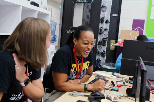
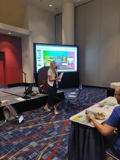
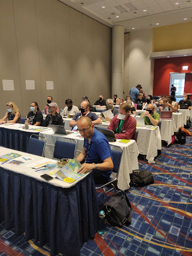
It was great to see the return of the Computer Science Teachers Association (CSTA) Annual Conference to an in-person event this year, and I was really excited to be able to attend.
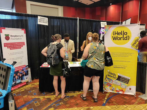
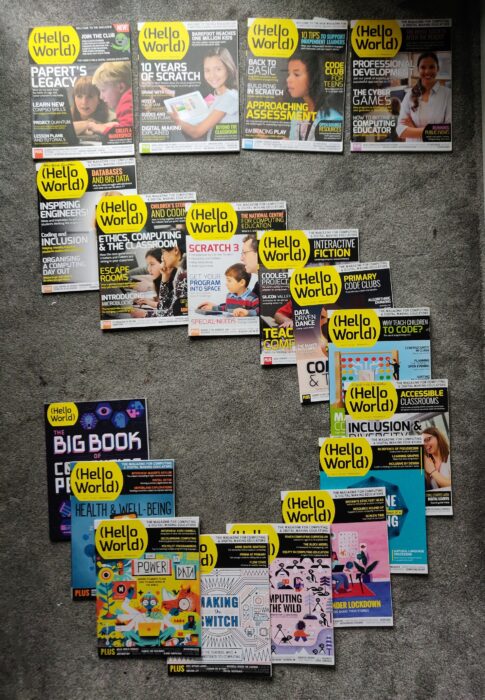
Our small Raspberry Pi Foundation team headed to Chicago for four and a half days of meetups, professional development, and conversations with educators from all across the US and around the world. Over the week our team ran workshops, delivered a keynote talk, gave away copies of Hello World magazine, and signed up many new subscribers. You too can subscribe to Hello World magazine for free at helloworld.cc/subscribe.
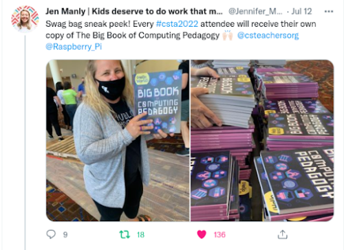
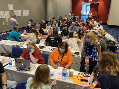
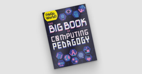
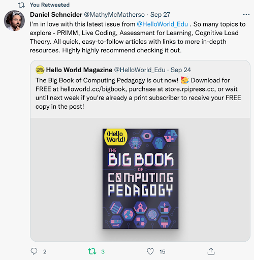
We spoke to so many educators about all parts of the Raspberry Pi Foundation’s work, with a particular focus on the Hello World magazine and podcast, and of course The Big Book of Computing Pedagogy. In collaboration with CSTA, we were really proud to be able to provide all attendees with their own physical copy of this very special edition.
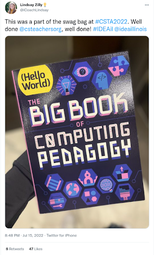
It was genuinely exciting to see how pleased attendees were to receive their copy of TheBig Book of Computing Pedagogy. So many came to talk to us about how they’d used the digital copy already and their plans for using the book for training and development initiatives in their schools and districts. We gave away every last spare copy we had to teachers who wanted to share the book with their colleagues who couldn’t attend.
Don’t worry if you couldn’t make it to the conference, The Big Book of Computing Pedagogy is available as a free PDF, which due to its Creative Commons licence you are welcome to print for yourself.
Another goal for us at CSTA was to support and encourage new authors to the magazine in order to ensure that Hello World continues to be the magazine for computing educators, by computing educators. Anyone can propose an article idea for Hello World by completing this form. We’re confident that every computing educator out there has at least one story to tell, lessons or learnings to share, or perhaps a cautionary tale of something that failed.
We’ll review any and all ideas and will support you to craft your idea into a finished article. This is exactly what we began to do at the conference with our workshop for writers led by Gemma Coleman, our fantastic Hello World Editor. We’re really excited to see these ideas flourish into full-blown articles over the coming weeks and months.
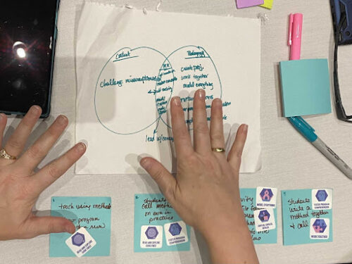
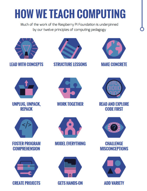
Our week culminated in a keynote talk delivered by Sue, Jane, and James, exploring how we developed our 12 pedagogy principles that underpin The Big Book of Computing Pedagogy, as well as much of the content we create at the Raspberry Pi Foundation. These principles are designed to describe a set of approaches that educators can add to their toolkit, giving them a shared language and the agency to select when and how they employ each approach. This was something we explored with teachers in our final breakout session where teachers applied these principles to describe a lesson or activity of their own.
We found the experience extremely valuable and relished the opportunity to talk about teaching and learning with educators and share our work. We are incredibly grateful to the entire CSTA team for organising a fantastic conference and inviting us to participate.
Discover more with Hello World — for free
Subscribe now to get each new Hello World straight to your digital inbox, for free! And if you’re based in the UK and do paid or unpaid work in education, you can subscribe for free print issues.
This year’s AWS re:Inforce conference in Boston has been jam-packed with thrilling speakers, deep insights on all things cloud, and some much-needed in-person collaboration from all walks of the technology community. It also coincides with some exciting announcements from AWS — and we’re honored to be a part of two of them. Here’s a look at how Rapid7 is building on our existing partnership with Amazon Web Services to help organizations securely advance in today’s cloud-native business landscape.
InsightIDR awarded AWS Security Competency
For seven years, AWS has issued security competencies to partners who have a proven track record of helping customers secure their AWS environments. Today at re:Inforce, AWS re-launched their Security Competency program, so that it better aligns with customers’ constantly evolving security challenges. Rapid7 is proud to be included in this re-launch, having obtained a security competency under the new criteria for its InsightIDR solution in the Threat Detection and Response category. This is Rapid7’s second AWS security competency and fourth AWS competency.
This designation recognizes that InsightIDR has demonstrated and successfully met AWS’s technical and quality requirements for providing customers with a deep level of software expertise in security incident and event management (SIEM), helping them achieve their cloud security goals.
InsightIDR integrates with a number of AWS services, including CloudTrail, GuardDuty, S3, VPC Traffic Mirroring, and SQS. InsightIDR’s UEBA feature includes dedicated AWS detections. The Insight Agent can be installed on EC2 instances for continuous monitoring. InsightIDR also features an out-of-the-box honeypot purpose-built for AWS environments. Taken together, these integrations and features give AWS customers the threat detection and response capabilities they need, all in a SaaS solution that can be deployed in a matter of weeks.
Adding another competency to Rapid7’s repertoire reaffirms our commitment to giving organizations the tools they need to innovate securely in a cloud-first world.
Rapid7 named a launch partner for AWS GuardDuty Malware Protection
Malware Protection is the new malware detection capability AWS has added to their GuardDuty service — and we’re honored to join them as a launch partner, with two products that support this new GuardDuty functionality.
GuardDuty is AWS’s threat detection service. It monitors AWS environments for suspicious behavior. Malware Protection introduces a new type of detection capability to GuardDuty. When GuardDuty fires an alert that’s related to an Amazon Elastic Cloud Compute (EC2) instance or a container running on EC2, Malware Protection will automatically run a scan on the instance in question and detect malware using machine learning and threat intelligence. When trojans, worms, rootkits, crypto miners, or other forms of malware are detected, they appear as new findings in GuardDuty, so security teams can take the right remediation actions.
Rapid7 customers can ingest GuardDuty findings (including the new malware detections) into InsightIDR and InsightCloudSec. In InsightIDR, each type of GuardDuty finding can be treated as a notable behavior or as an alert which will automatically trigger a new investigation. This allows security teams to know the instant suspicious activity is detected in their AWS environment and react accordingly. Should an investigation be triggered, teams can use InsightIDR’s native automation capabilities to enrich the data from GuardDuty, quarantine a user, and more. In the case where GuardDuty detects malware, teams can pull additional data from the Insight agent and even terminate malicious processes. In addition, customers can use InsightIDR’s Dashboards capability to keep an eye on GuardDuty and spot trends in the findings.
InsightCloudSec customers can likewise build automated bots that automatically react to GuardDuty findings. When GuardDuty has detected malware, a customer might configure a bot that terminates the infected instance. Alternatively, a customer might choose to reconfigure the instance’s security group to effectively isolate it while the team investigates. The options are practically endless.
Rapid7 and AWS continue to deepen partnership to protect your cloud workloads
AWS re:Inforce 2022 provides a welcome opportunity for the community to come together and share insights about managing and securing cloud environments, and we can’t think of better timing to announce these two areas of partnership with AWS. Click here to learn more about what we’re up to at this year’s AWS re:Inforce conference in Boston.
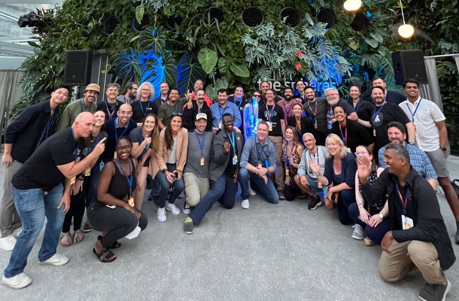
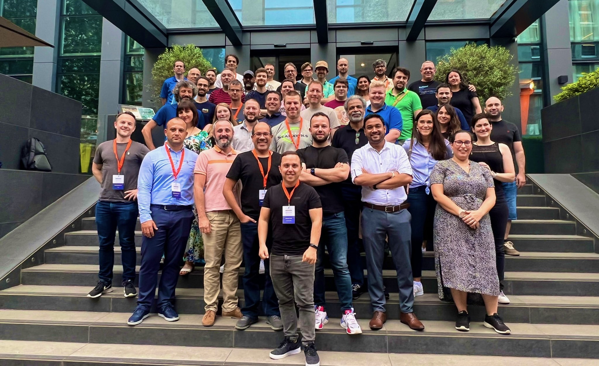
A few weeks ago, we hosted the first EMEA AWS Heroes Summit in Milan, Italy. This past week, I had the privilege to join the Americas AWS Heroes Summit in Seattle, Washington, USA. Meeting with our community experts is always inspiring and a great opportunity to learn from each other. During the Summit, AWS Heroes from North America and Latin America shared their thoughts with AWS developer advocates and product teams on topics such as serverless, containers, machine learning, data, and DevTools. You can learn more about the AWS Heroes program here.
Last Week’s Launches Here are some launches that got my attention during the previous week:
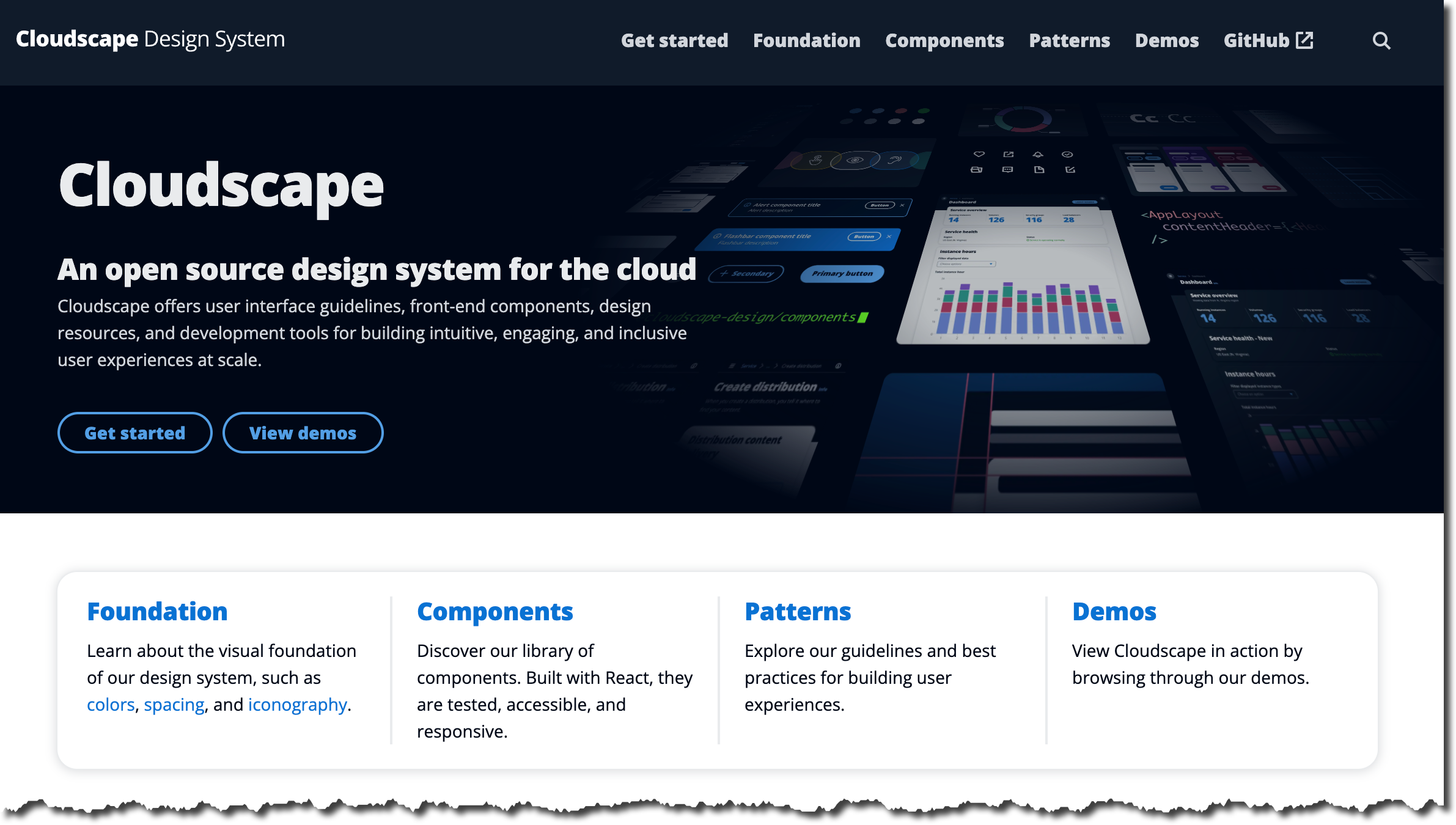
Cloudscape Design System – Cloudscape is an open source design system for creating web applications. It was built for and is used by AWS products and services. We created it in 2016 to improve the user experience across web applications owned by AWS services and also to help teams implement those applications faster. If you’ve ever used the AWS Management Console, you’ve seen Cloudscape in action. If you are building a product that extends the AWS Management Console, designing a user interface for a hybrid cloud management system, or setting up an on-premises solution that uses AWS, have a look at Cloudscape Design System.
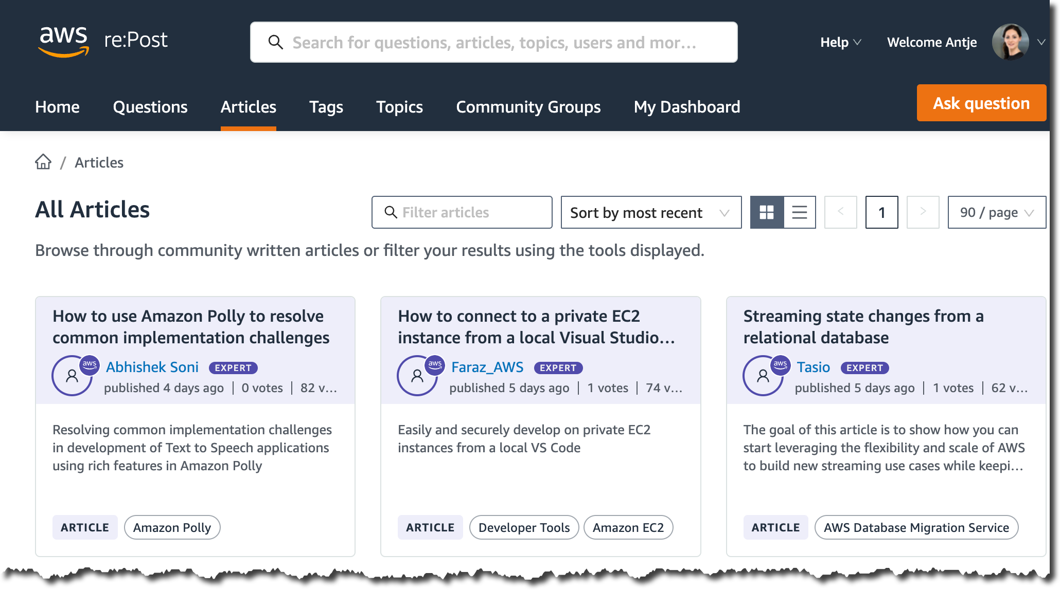
AWS re:Post introduces community-generated articles – AWS re:Post gives you access to a vibrant community that helps you become even more successful on AWS. Expert community members can now share technical guidance and knowledge beyond answering questions through the Articles feature. Using this feature, community members can share best practices and troubleshooting processes and address customer needs around AWS technology in greater depth. The Articles feature is unlocked for community members who have achieved Rising Star status on re:Post or subject matter experts who built their reputation in the community based on their contributions and certifications. If you have a Rising Star status on re:Post, start writing articles now! All other members can unlock Rising Star status through community contributions or simply browse available articles today on re:Post.
AWS Lambda announces support for attribute-based access control (ABAC) and new IAM condition key – You can now use attribute-based access control (ABAC) with AWS Lambda to control access to functions within AWS Identity and Access Management (IAM) using tags. ABAC is an authorization strategy that defines access permissions based on attributes. In AWS, these attributes are called tags. With ABAC, you can scale an access control strategy by setting granular permissions with tags without requiring permissions updates for every new user or resource as your organization scales. Read this blog post by Julian Wood and Chris McPeek to learn more.
AWS Lambda also announced support for lambda:SourceFunctionArn, a new IAM condition key that can be used for IAM policy conditions that specify the Amazon Resource Name (ARN) of the function from which a request is made. You can use the Condition element in your IAM policy to compare the lambda:SourceFunctionArn condition key in the request context with values that you specify in your policy. This allows you to implement advanced security controls for the AWS API calls taken by your Lambda function code. For more details, have a look at the Lambda Developer Guide.
Amazon Fraud Detector launches Account Takeover Insights (ATI) – Amazon Fraud Detector now supports an Account Takeover Insights (ATI) model, a low-latency fraud detection machine learning model specifically designed to detect accounts that have been compromised through stolen credentials, phishing, social engineering, or other forms of account takeover. The ATI model is designed to detect up to four times more ATI fraud than traditional rules-based account takeover solutions while minimizing the level of friction for legitimate users. To learn more, have a look at the Amazon Fraud Detector documentation.
Amazon EMR on EC2 clusters (EMR Clusters) introduces more fine-grained access controls – Previously, all jobs running on an EMR cluster used the IAM role associated with the EMR cluster’s EC2 instances to access resources. This role is called the EMR EC2 instance profile. With the new runtime roles for Amazon EMR Steps, you can now specify a different IAM role for your Apache Spark and Hive jobs, scoping down access at a job level. This simplifies access controls on a single EMR cluster that is shared between multiple tenants, wherein each tenant is isolated using IAM roles. You can now also enforce table and column permissions based on your Amazon EMR runtime role to manage your access to data lakes with AWS Lake Formation. For more details, read the What’s New post.
Other AWS News Here are some additional news and customer stories you may find interesting:
AWS open-source news and updates – My colleague Ricardo Sueiras writes this weekly open-source newsletter in which he highlights new open-source projects, tools, and demos from the AWS Community. Read edition #121 here.
AI Use Case Explorer – If you are interested in AI use cases, have a look at the new AI Use Case Explorer. You can search over 100 use cases and 400 customer success stories by industry, business function, and the business outcome you want to achieve.
Bayer centralizes and standardizes data from the carbon program using AWS – To help Brazilian farmers adopt climate-smart agricultural practices and reduce carbon emissions in their activities, Bayer created the Carbon Program, which aims to build carbon-neutral agriculture practices. Learn how Bayer uses AWS to centralize and standardize the data received from the different partners involved in the project in this Bayer case study.
Upcoming AWS Events Check your calendars and sign up for these AWS events:
AWS Global Summits – AWS Global Summits are free events that bring the cloud computing community together to connect, collaborate, and learn about AWS. Registrations are open for the following AWS Summits in August:
IMAGINE 2022 – The IMAGINE 2022 conference will take place on August 3 at the Seattle Convention Center, Washington, USA. It’s a no-cost event that brings together education, state, and local leaders to learn about the latest innovations and best practices in the cloud. You can register here.
I’ll be speaking at Data Con LA on August 13–14 in Los Angeles, California, USA. Feel free to say “Hi!” if you’re around. And if you happen to be at Ray Summit on August 23–24 in San Francisco, California, USA, stop by the AWS booth. I’ll be there to discuss all things Ray on AWS.
That’s all for this week. Check back next Monday for another Week in Review!
Last week, AWS Summit New York was held in person at the Javits Center with thousands of attendees and over 100 sponsors and partners. During the keynote, Martin Beeby, AWS Principal Developer Advocate, talked about how innovations in cloud infrastructure enable customers to adapt to challenges and seize new opportunities. It included Liz Fong-Jones‘s great migration story of AWS Graviton in Honeycomb and Elliott Cordo‘s story of improving pharmacy experiences using AWS analytics and machine learning services in Capsule.
A Recap of AWS Summit NY Announcements During the keynote, we announced the general availability of some new services:
Amazon Redshift Serverless – This serverless option lets you analyze data at any scale without having to manage data warehouse infrastructure. You can now create multiple serverless endpoints per AWS account and Region using namespaces and workgroups and enjoy reducing serverless compute costs compared to the preview. To learn more, check out Danilio’s blog post, this demo video, and the latest episode of The Official AWS Podcast. We also introduced new features of row-level security (RLS), which implement fine-grained access to the rows in tables, and automated materialized view to lower query latency for repeatable workloads.
AWS Cloud WAN – This new network service makes it easy to build and operate wide area networks (WAN) that connect your data centers and branch offices, as well as multiple VPCs in multiple AWS Regions. To learn more, read Seb’s blog post.
Amazon DevOps Guru’s Log Anomaly Detection and Recommendations – This new feature identifies anomalies such as increased latency, error rates, and resource constraints within your app and then sends alerts with a description and actionable recommendations for remediation. To learn more, see Donnie’s blog post as a new News Blog writer.
Last Week’s Launches Here are some other launches that caught my attention last week:
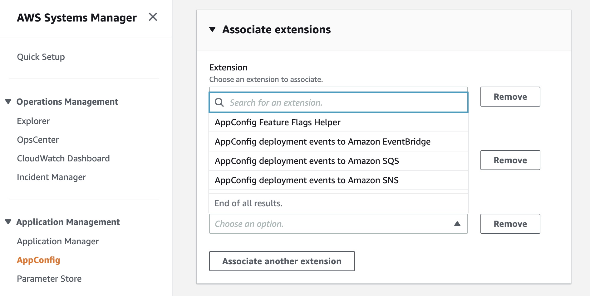
AWS AppConfig, a feature of AWS Systems Manager, makes it easy for customers to quickly and safely configure, validate, and deploy feature flags and application configuration. Now, we have announced AWS AppConfig Extensions, a new capability that allows customers to enhance and extend the capabilities of feature flags and dynamic runtime configuration data.
Available extensions at launch include AppConfig Notification extensions that push messages about configuration updates to Amazon EventBridge, Amazon SNS, Amazon SQS, or a Jira extension to track Feature Flag changes in AppConfig as Atlassian’s Jira issues. To get started, read Announcing AWS AppConfig Extensions and AppConfig Extensions.
Amazon VPC Flow Logs for Transit Gateway is a new capability that allows customers to gain deeper visibility and insights into network traffic on AWS Transit Gateway. With this feature, Transit Gateway can export detailed information, such as source/destination IPs, ports, protocols, traffic counters, timestamps, and various metadata for all of the network flow traversing through the Transit Gateway. To learn more, read Introducing VPC Flow Logs for AWS Transit Gateway and Logging network traffic using Transit Gateway Flow Logs.
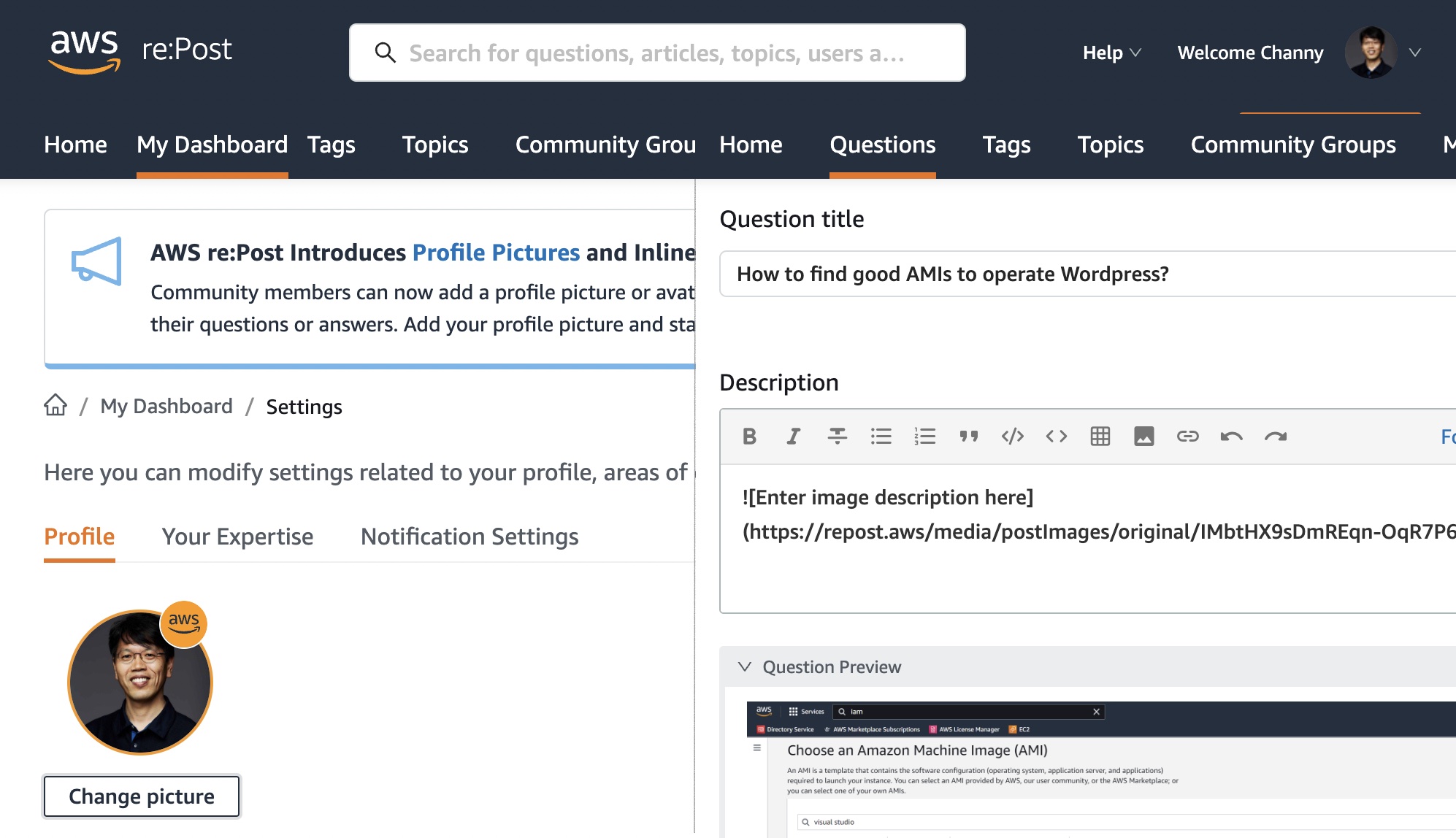
AWS re:Post is a vibrant Q&A community that helps you become even more successful on AWS. You can now add a profile picture or avatar to your account and add inline images such as diagrams or screenshots to support your questions or answers. Add your profile picture and start using inline images today!
Other AWS News Here are some news, blog posts, and video series for you to know:
In July 2021, we notified users about the end of support for Internet Explorer 11, which is now approaching on July 31, 2022. The browser will no longer be supported in the AWS Management Console, web-based services such as Amazon QuickSight, Amazon Chime, Amazon Honeycode, and some other AWS websites. After that date, we can no longer guarantee that the features and webpages will function properly on IE 11. For more information, please visit AWS Supported Browsers.
In fall 2021, we began offering a free multi-factor authentication (MFA) security key to AWS account owners in the United States. Now eligible customers can order the free MFA security key through the ordering portal in the AWS Management Console. At this time, only U.S.-based AWS account root users who have spent more than $100 each month over the past 3 months are eligible to place an order. For more information, see our Free MFA Security Key page.
Amazon’s Machine Learning University expands with MLU Explains, a public website containing visual essays that incorporate fun animations and scrollytelling to explain machine learning concepts in an accessible manner. The following animation teaches the concepts of data splitting in machine learning using an example model that attempts to determine whether animals are cats or dogs. To learn more, read the Amazon Science blog post.
This is My Architecture is a video series that showcases innovative architectural solutions on the AWS Cloud by customers and partners. In June and July, over 15 episodes were updated, including GoDaddy, Riot Games, and Hudl. Each episode examines the most interesting and technically creative elements of each cloud architecture.
Upcoming AWS Events in August Check your calendars and sign up for these AWS events:
Registration is open for upcoming in-person AWS Summits that might be close to you in August: Sao Paulo (August 3–4), Anaheim (August 18), Taiwan (August 10–11), Chicago (August 28), and Canberra (August 31).
AWS Innovate – Data Edition – On August 23, learn how a modern data strategy can support your present and future use cases, including steps to build an end-to-end data solution to store and access, analyze and visualize, and even predict.
AWS Innovate – For Every Application Edition – On August 25, learn about a wide selection of AWS solutions across compute, storage, networking, hybrid, and edge infrastructure to help you scale application resources seamlessly and optimally.
Although these two Innovate events will be held in Asia Pacific and Japan time zones, you can view on-demand videos for two months following your registration.
If you’re interested in learning modern development practices live in New York City, I recommend joining AWS Solutions Day on August 10. I love advanced topics to focus on building new web apps with Java, JavaScript, TypeScript, and GraphQL.
If you’re interested in learning AWS fundamentals and preparing for AWS Certifications, there are several virtual events in August, such as AWS Cloud Practitioner Essentials Day, AWS Technical Essentials Day, and Exam Readiness for AWS Certificates.
That’s all for this week. Check back next Monday for another Week in Review!
Register now with discount code SALUZwmdkJJ to get $150 off your full conference pass to AWS re:Inforce. For a limited time only and while supplies last.
Today we want to tell you about some of the exciting governance, risk, and compliance sessions planned for AWS re:Inforce 2022. AWS re:Inforce is a conference where you can learn more about security, compliance, identity, and privacy. When you attend the event, you have access to hundreds of technical and business sessions, an AWS Partner expo hall, a keynote speech from AWS Security leaders, and more. AWS re:Inforce 2022 will take place in person in Boston, MA on July 26 and 27. AWS re:Inforce 2022 features content in the following five areas:
Data protection and privacy
Governance, risk, and compliance
Identity and access management
Network and infrastructure security
Threat detection and incident response
This post will highlight of some of the governance, risk, and compliance offerings that you can sign up for, including breakout sessions, chalk talks, builders’ sessions, and workshops. For the full catalog of all tracks, see the AWS re:Inforce session preview.
Breakout sessions
These are lecture-style presentations that cover topics at all levels and are delivered by AWS experts, builders, customers, and partners. Breakout sessions typically include 10–15 minutes of Q&A at the end.
GRC201: Learn best practices for auditing AWS with Cloud Audit Academy Do you want to know how to audit in the cloud? Today, control framework language is catered toward on-premises environments, and security IT auditing techniques have not been reshaped for the cloud. The AWS Cloud–specific Cloud Audit Academy provides auditors with the education and tools to audit for security on AWS using a risk-based approach. In this session, experience a condensed sample domain from a four-day Cloud Audit Academy workshop.
GRC203: Panel discussion: Continuous compliance and auditing on AWS In this session, an AWS leader speaks with senior executives from enterprise customer and AWS Partner organizations as they share their paths to success with compliance and auditing on AWS. Join this session to hear how they have used AWS Cloud Operations to help make compliance and auditing more efficient and improve business outcomes. Also hear how AWS Partners are supporting customer organizations as they automate compliance and move to the cloud.
GRC205: Crawl, walk, run: Accelerating security maturity Where are you on your cloud security journey? Where do you want to end up? What are your next steps? In this step-by-step roadmap, we provide a comprehensive overview of the AWS security journey based on lessons learned with other organizations. Learn where you are, how to take the next step and how to improve your cloud security program. In this session, we will leverage cloud-native tools like AWS Control Tower, AWS Config, and AWS Security Hub to demonstrate how knowing your current state of security can drive more effective and efficient story telling of your posture.
GRC302: Using AWS security services to build our cloud operations foundation Organizations new to the cloud need to quickly understand what foundational security capabilities should be considered as a baseline. In this session, learn how AWS security services can help you improve your cloud security posture. Learn how to incorporate security into your AWS architecture based on the AWS Cloud Operations model, which will help you implement governance, manage risk, and achieve compliance while proactively discovering opportunities for improvement.
GRC331: Automating security and compliance with OSCAL Documentation exports can be very time consuming. In this session, learn how the National Institute of Science and Technology is developing the Open Security Controls Assessment Language (OSCAL) to provide common translation between XML, JSON, and YAML formats. OSCAL also provides a common means to identify and version shared resources, and standardize the expression of assessment artifacts. Learn how AWS is working to implement OSCAL for our security documentation exports so that you can save time when creating and maintaining ATO packages.
Builders’ sessions
These are small-group sessions led by an AWS expert who guides you as you build the service or product on your own laptop. Use your laptop to experiment and build along with the AWS expert.
GRC351: Implementing compliance as code on AWS To manage compliance at the speed and scale the cloud requires, organizations need to implement automation and have an effective mechanism to manage it. In this builders’ session, learn how to implement compliance as code (CaC). CaC shares many of the same benefits as infrastructure as code: speed, automation, peer review, and auditability. Learn about defining controls with AWS Config rules, customizing those controls, using remediation actions, packaging and deploying with AWS Config conformance packs, and validating using a CI/CD pipeline.
GRC352: Deploying repeatable, secure, and compliant Amazon EKS clusters In this builders’ session, learn how to deploy, manage, and scale containerized applications that run Kubernetes on AWS with AWS Service Catalog. Walk through how to deploy the Kubernetes control plane into a virtual private cloud (VPC), connect worker nodes to the cluster, and configure a bastion host for cluster administrative operations. Using AWS CloudFormation registry resource types, learn how to declare Kubernetes manifests or Helm charts to deploy and manage your Kubernetes applications. With AWS Service Catalog, you can empower your teams to deploy securely configured Amazon Elastic Kubernetes Service (Amazon EKS) clusters in multiple accounts and Regions.
GRC354: Building remediation workflows to simplify compliance Automation and simplification are key to managing compliance at scale. Remediation is one of the key elements of simplifying and managing risk. In this builders’ session, walk through how to build a remediation workflow using AWS Config and AWS Systems Manager Automation. Then, explore how the workflow can be deployed at scale and monitored with AWS Security Hub to oversee your entire organization.
GRC355: Build a Security Posture Leaderboard using AWS Security Hub This builders’ session introduces you to the possibilities of creating a robust and comprehensive leaderboard using AWS Security Hub findings to improve security and compliance visibility in your organization. Learn how to design and support various use cases, such as combining security and compliance data into a single, centralized dashboard that allows you to make more informed decisions; correlating Security Hub findings with operational data for deeper insights; building a security and compliance scorecard across various dimensions to share across different stakeholders; and supporting a decentralized organization structure with centralized or shared security function.
Chalk talks
These are highly interactive sessions with a small audience. Experts lead you through problems and solutions on a digital whiteboard as the discussion unfolds.
GRC233: Critical infrastructure: Supply chain and compliance impacts In this chalk talk, learn how you can benefit from cloud-based solutions that build in security from the beginning. Review technical details around cybersecurity best practices for OT systems in adherence with government partnership with public and private industries. Dive deep into use cases and best practices for using AWS security services to help improve cybersecurity specifically for water utilities. Hear about opportunities to receive AWS cybersecurity training designed to teach you the skills necessary to support cloud adoption.
GRC304: Scaling the possible: Digitizing the audit experience Do you want to increase the speed and scale of your audits? As companies expand to new industries and environments, so too does the scale of regulatory compliance. AWS undergoes over 500 audits in a year. In this session, hear from AWS experts as they digitize and automate the regulator/auditor experience. Walk through pre-audit educational training, self-service of control evidence and walkthrough information, live chatting with an audit control owner, and virtual data center tours. This session discusses how innovation and digitization allows companies to build trust with regulators and auditors while reducing the level of effort for internal audit teams and compliance executives.
GRC334: Shared responsibility deep dive at the service level Auditors and regulators often need assistance understanding which configuration settings and security responsibilities are in the company’s control. Depending on the service, the AWS shared responsibility model can vary, which can affect the process for meeting compliance goals. Join AWS subject-matter experts in this chalk talk for an in-depth discussion on the next wave of compliance activation for AWS customers. Explore the configurable security decisions that users have for each service and how you can map to AWS best practices and security controls.
GRC431: Building purpose-driven and data-rich GRC solutions Are you getting everything you need out of your data? Or do you not have enough information to make data-driven security decisions? Many organizations trying to modernize and innovate using data often struggle with finding the right data security solutions to build data-driven applications. In this chalk talk, explore how you can use Amazon Virtual Private Cloud (Amazon VPC), AWS Identity and Access Management (IAM), AWS Key Management Service (AWS KMS), AWS Systems Manager, AWS Single Sign-On (AWS SSO), and AWS Config to drive valuable insights to make more informed decisions. Hear about best practices and lessons learned to help you on your journey to garner purpose-filled information.
Workshops
These are interactive learning sessions where you work in small teams to solve problems using AWS Cloud security services. Come prepared with your laptop and a willingness to learn!
GRC272: Executive Security Simulation The Executive Security Simulation takes senior security management and IT/business executive teams through an experiential exercise that illuminates key decision points for a successful and secure cloud journey. During this team-based, game-like competitive simulation, participants leverage an industry case study to make strategic security, risk, and compliance time-based decisions and investments. Participants experience the impact of these investments and decisions on the critical aspects of their secure cloud adoption. Join this workshop to understand the major success factors to lead security, risk, and compliance in the cloud, and learn applicable decision and investment approaches to specific secure cloud adoption journeys.
GRC371: Automate your compliance and evidence collection with AWS Automation and simplification are key to managing compliance at scale. Remediation is one of the key elements of simplifying and managing risk. In this workshop, we will walk through building a remediation workflow using AWS Config and AWS Systems Manager and show how it can be deployed at scale and then monitored with Security Hub across the entire organization. In this workshop, you will learn how you can set up a continuous collection process that not only establishes controls to help meet the requirements of compliance but also automates the process of collecting evidence to avoid the time-consuming manual effort to prepare for audits.
GRC372: How to implement governance on AWS with ServiceNow Many AWS customers use IT service management (ITSM) solutions such as ServiceNow to implement governance and compliance and manage security incidents. In this workshop, learn how to use AWS services such as AWS Service Catalog, AWS Config, AWS Systems Manager, and AWS Security Hub on the ServiceNow service portal. Learn how AWS services align to service management standards by integrating AWS capabilities through ITSM process integration with ServiceNow. Design and implement a curated provisioning strategy, along with incident management and resource transparency/compliance, by using the AWS Service Management Connector for ServiceNow.
GRC471: Building guardrails to meet your custom control requirements In this session, you will experience the process of identifying, designing, and implementing security configurations, as well as detective and preventive guardrails, to meet custom control requirements. You will use a pre-built environment, read a customer scenario to identify specific control needs, and then learn how to design and implement the custom controls.
If any of these sessions look interesting to you, consider joining us in Boston by registering for re:Inforce 2022. We look forward to seeing you there!
In France, we know summer has started when you see the Tour de France bike race on TV or in a city nearby. This year, the tour stopped in the city where I live, and I was blocked on my way back home from a customer conference to let the race pass through.
It’s Monday today, so let’s make another tour—a tour of the AWS news, announcements, or blog posts that captured my attention last week. I selected these as being of interest to IT professionals and developers: the doers, the builders that spend their time on the AWS Management Console or in code.
Last Week’s Launches Here are some launches that got my attention during the previous week:
Amazon EC2 Mac M1 instances are generally available – this new EC2 instance type allows you to deploy Mac mini computers with M1 Apple Silicon running macOS using the same console, API, SDK, or CLI you are used to for interacting with EC2 instances. You can start, stop them, assign a security group or an IAM role, snapshot their EBS volume, and recreate an AMI from it, just like with Linux-based or Windows-based instances. It lets iOS developers create full CI/CD pipelines in the cloud without requiring someone in your team to reinstall various combinations of macOS and Xcode versions on on-prem machines. Some of you had the chance the enter the preview program for EC2 Mac M1 instances when we announced it last December. EC2 Mac M1 instances are now generally available.
A streamlined deployment experience for .NET applications –the new deployment experience focuses on the type of application you want to deploy instead of individual AWS services by providing intelligent compute recommendations. You can find it in the AWS Toolkit for Visual Studio using the new “Publish to AWS” wizard. It is also available via the .NET CLI by installing AWS Deploy Tool for .NET. Together, they help easily transition from a prototyping phase in Visual Studio to automated deployments. The new deployment experience supports ASP.NET Core, Blazor WebAssembly, console applications (such as long-lived message processing services), and tasks that need to run on a schedule.
Other AWS News This week, I also learned from these blog posts:
TLS 1.2 to become the minimum TLS protocol level for all AWS API endpoints – this article was published at the end of June, and it deserves more exposure. Starting in June 2022, we will progressively transition all our API endpoints to TLS 1.2 only. The good news is that 95 percent of the API calls we observe are already using TLS 1.2, and only five percent of the applications are impacted. If you have applications developed before 2014 (using a Java JDK before version 8 or .NET before version 4.6.2), it is worth checking your app and updating them to use TLS 1.2. When we detect your application is still using TLS 1.0 or TLS 1.1, we inform you by email and in the AWS Health Dashboard. The blog article goes into detail about how to analyze AWS CloudTrail logs to detect any API call that would not use TLS 1.2.
How to implement automated appointment remindersusing Amazon Connect and Amazon Pinpoint – this blog post guides you through the steps to implement a system to automatically call your customers to remind them of their appointments. This automated outbound campaign for appointment reminders checked the campaign list against a “do not call” list before making an outbound call. Your customers are able to confirm automatically or reschedule by speaking to an agent. You monitor the results of the calls on a dashboard in near real time using Amazon QuickSight. It provides you with AWS CloudFormation templates for the parts that can be automated and detailed instructions for the manual steps.
Using Amazon CloudWatch metrics math to monitor and scale resources – AWS Auto Scaling is one of those capabilities that may look like magic at first glance. It uses metrics to take scale-out or scale-in decisions. Most customers I talk with struggle a bit at first to define the correct combination of metrics that allow them to scale at the right moment. Scaling out too late impacts your customer experience while scaling out too early impacts your budget. This article explains how to use metric math, a way to query multiple Amazon CloudWatch metrics, and use math expressions to create new time series based on these metrics. These math metrics may, in turn, be used to trigger scaling decisions. The typical use case would be to mathematically combine CPU, memory, and network utilization metrics to decide when to scale in or to scale out.
How to use Amazon RDS and Amazon Aurora with a static IP address – in the cloud, it is better to access network resources by referencing their DNS name instead of IP addresses. IP addresses come and go as resources are stopped, restarted, scaled out, or scaled in. However, when integrating with older, more rigid environments, it might happen, for a limited period of time, to authorize access through a static IP address. You have probably heard that scary phrase: “I have to authorize your IP address in my firewall configuration.” This new blog post explains how to do so for Amazon Relational Database Service (Amazon RDS) database. It uses a Network Load Balancer and traffic forwarding at the Linux-kernel level to proxy your actual database server.
Summer has arrived in Finland, and these last few days have been hotter than in the Canary Islands! Today in the US it is Independence Day. I hope that if you are celebrating, you’re having a great time. This week I’m very excited about some developer experience and artificial intelligence launches.
Last Week’s Launches Here are some launches that got my attention during the previous week:
AWS SAM Accelerate is now generally available – SAM Accelerate is a new capability of the AWS Serverless Application Model CLI, which makes it easier for serverless developers to test code changes against the cloud. You can do a hot swap of code directly in the cloud when making a change in your local development environment. This allows you to develop applications faster. Learn more about this launch in the What’s New post.
Amplify UI for React is generally available – Amplify UI is an open-source UI library that helps developers build cloud-native applications. Amplify UI for React comes with over 35 components that you can use, an authentication component that allows you to connect to your backend with no extra configuration, theming for your components. You can also build your UI using Figma. Check the Amplify UI for React site to learn more about all the capabilities offered.
Other AWS News Some other updates and news that you may have missed:
AWS Support announced an improved experience when creating a case – There is a new interface for creating support cases in the AWS Support Center console. Now you can create a case with a simplified three-step process that guides you through the flow. Learn more about this new process in the What’s new post.
New AWS Step Functions workflows collection on Serverless Land – The Step Functions workflows collection is a new experience that makes it easier to discover, deploy, and share AWS Step Functions workflows. In this collection, you can find opinionated templates that implement the best practices to build using Step Functions. Learn more about this new collection in Ben’s blog post.
Podcast Charlas Técnicas de AWS – If you understand Spanish, this podcast is for you. Podcast Charlas Técnicas is one of the official AWS Podcasts in Spanish, which shares a new episode ever other week. The podcast is meant for builders, and it shares stories about how customers implement and learn AWS, how to architect applications, and how to use new services. You can listen to all the episodes directly from your favorite podcast app or from the AWS Podcasts en español website.
AWS open-source news and updates – A newsletter curated by my colleague Ricardo brings you the latest open-source projects, posts, events, and more.
Upcoming AWS Events Check your calendars and sign up for these AWS events:
AWS Summit New York – Join us on July 12 for the in-person AWS Summit. You can register on the AWS Summit page for free.
AWS re:Inforce – This is an in-person learning conference with a focus on security, compliance, identity, and privacy. You can register now to access hundreds of technical sessions, and other content. It will take place July 26 and 27 in Boston, MA.
That’s all for this week. Check back next Monday for another Week in Review!
It’s the beginning of a new week, and I’d like to start with a recap of the most significant AWS news from the previous 7 days. Last week was special because I had the privilege to be at the very first EMEA AWS Heroes Summit in Milan, Italy. It was a great opportunity of mutual learning as this community of experts shared their thoughts with AWS developer advocates, product managers, and technologists on topics such as containers, serverless, and machine learning.
Last Week’s Launches Here are the launches that got my attention last week:
Private IP VPNs with AWS Site-to-Site VPN – You can now deploy AWS Site-to-Site VPN connections over AWS Direct Connectusing private IP addresses. This way, you can encrypt traffic between on-premises networks and AWS via Direct Connect connections without the need for public IP addresses.
AWS Center for Quantum Networking – Research and development of quantum computers have the potential to revolutionize science and technology. To address fundamental scientific and engineering challenges and develop new hardware, software, and applications for quantum networks, we announced the AWS Center for Quantum Networking.
Synthetic data generation with Amazon SageMaker Ground Truth – Generate labeled synthetic image data that you can combine with real-world data to create more complete training datasets for your ML models.
Large object storage strategies for Amazon DynamoDB – A blog post showing different options for handling large objects within DynamoDB and the benefits and disadvantages of each approach.
Register now with discount code SALXTDVaB7y to get $150 off your full conference pass to AWS re:Inforce. For a limited time only and while supplies last.
Today we’re going to highlight just some of the sessions focused on threat detection and incident response that are planned for AWS re:Inforce 2022. AWS re:Inforce is a learning conference focused on security, compliance, identity, and privacy. The event features access to hundreds of technical and business sessions, an AWS Partner expo hall, a keynote featuring AWS Security leadership, and more. AWS re:Inforce 2022 will take place in-person in Boston, MA on July 26-27.
AWS re:Inforce organizes content across multiple themed tracks: identity and access management; threat detection and incident response; governance, risk, and compliance; networking and infrastructure security; and data protection and privacy. This post highlights some of the breakout sessions, chalk talks, builders’ sessions, and workshops planned for the threat detection and incident response track. For additional sessions and descriptions, see the re:Inforce 2022 catalog preview. For other highlights, see our sneak peek at the identity and access management sessions and sneak peek at the data protection and privacy sessions.
Breakout sessions
These are lecture-style presentations that cover topics at all levels and delivered by AWS experts, builders, customers, and partners. Breakout sessions typically include 10–15 minutes of Q&A at the end.
TDR201: Running effective security incident response simulations Security incidents provide learning opportunities for improving your security posture and incident response processes. Ideally you want to learn these lessons before having a security incident. In this session, walk through the process of running and moderating effective incident response simulations with your organization’s playbooks. Learn how to create realistic real-world scenarios, methods for collecting valuable learnings and feeding them back into implementation, and documenting correction-of-error proceedings to improve processes. This session provides knowledge that can help you begin checking your organization’s incident response process, procedures, communication paths, and documentation.
TDR202: What’s new with AWS threat detection services AWS threat detection teams continue to innovate and improve the foundational security services for proactive and early detection of security events and posture management. Keeping up with the latest capabilities can improve your security posture, raise your security operations efficiency, and reduce your mean time to remediation (MTTR). In this session, learn about recent launches that can be used independently or integrated together for different use cases. Services covered in this session include Amazon GuardDuty, Amazon Detective, Amazon Inspector, Amazon Macie, and centralized cloud security posture assessment with AWS Security Hub.
TDR301: A proactive approach to zero-days: Lessons learned from Log4j In the run-up to the 2021 holiday season, many companies were hit by security vulnerabilities in the widespread Java logging framework, Apache Log4j. Organizations were in a reactionary position, trying to answer questions like: How do we figure out if this is in our environment? How do we remediate across our environment? How do we protect our environment? In this session, learn about proactive measures that you should implement now to better prepare for future zero-day vulnerabilities.
TDR303: Zoom’s journey to hyperscale threat detection and incident response Zoom, a leader in modern enterprise video communications, experienced hyperscale growth during the pandemic. Their customer base expanded by 30x and their daily security logs went from being measured in gigabytes to terabytes. In this session, Zoom shares how their security team supported this breakneck growth by evolving to a centralized infrastructure, updating their governance process, and consolidating to a single pane of glass for a more rapid response to security concerns. Solutions used to accomplish their goals include Splunk, AWS Security Hub, Amazon GuardDuty, Amazon CloudWatch, Amazon S3, and others.
Builders’ sessions
These are small-group sessions led by an AWS expert who guides you as you build the service or product on your own laptop.
TDR351: Using Kubernetes audit logs for incident response automation In this hands-on builders’ session, learn how to use Amazon CloudWatch and Amazon GuardDuty to effectively monitor Kubernetes audit logs—part of the Amazon EKS control plane logs—to alert on suspicious events, such as an increase in 403 Forbidden or 401 Unauthorized Error logs. Also learn how to automate example incident responses for streamlining workflow and remediation.
TDR352: How to mitigate the risk of ransomware in your AWS environment Join this hands-on builders’ session to learn how to mitigate the risk from ransomware in your AWS environment using the NIST Cybersecurity Framework (CSF). Choose your own path to learn how to protect, detect, respond, and recover from a ransomware event using key AWS security and management services. Use Amazon Inspector to detect vulnerabilities, Amazon GuardDuty to detect anomalous activity, and AWS Backup to automate recovery. This session is beneficial for security engineers, security architects, and anyone responsible for implementing security controls in their AWS environment.
Chalk talks
Highly interactive sessions with a small audience. Experts lead you through problems and solutions on a digital whiteboard as the discussion unfolds.
TDR231: Automated vulnerability management and remediation for Amazon EC2 In this chalk talk, learn about vulnerability management strategies for Amazon EC2 instances on AWS at scale. Discover the role of services like Amazon Inspector, AWS Systems Manager, and AWS Security Hub in vulnerability management and mechanisms to perform proactive and reactive remediations of findings that Amazon Inspector generates. Also learn considerations for managing vulnerabilities across multiple AWS accounts and Regions in an AWS Organizations environment.
TDR332: Response preparation with ransomware tabletop exercises Many organizations do not validate their critical processes prior to an event such as a ransomware attack. Through a security tabletop exercise, customers can use simulations to provide a realistic training experience for organizations to test their security resilience and mitigate risk. In this chalk talk, learn about Amazon Managed Services (AMS) best practices through a live, interactive tabletop exercise to demonstrate how to execute a simulation of a ransomware scenario. Attendees will leave with a deeper understanding of incident response preparation and how to use AWS security tools to better respond to ransomware events.
Workshops
These are interactive learning sessions where you work in small teams to solve problems using AWS Cloud security services. Come prepared with your laptop and a willingness to learn!
TDR271: Detecting and remediating security threats with Amazon GuardDuty This workshop walks through scenarios covering threat detection and remediation using Amazon GuardDuty, a managed threat detection service. The scenarios simulate an incident that spans multiple threat vectors, representing a sample of threats related to Amazon EC2, AWS IAM, Amazon S3, and Amazon EKS, that GuardDuty is able to detect. Learn how to view and analyze GuardDuty findings, send alerts based on the findings, and remediate findings.
TDR371: Building an AWS incident response runbook using Jupyter notebooks This workshop guides you through building an incident response runbook for your AWS environment using Jupyter notebooks. Walk through an easy-to-follow sample incident using a ready-to-use runbook. Then add new programmatic steps and documentation to the Jupyter notebook, helping you discover and respond to incidents.
TDR372: Detecting and managing vulnerabilities with Amazon Inspector Join this workshop to get hands-on experience using Amazon Inspector to scan Amazon EC2 instances and container images residing in Amazon Elastic Container Registry (Amazon ECR) for software vulnerabilities. Learn how to manage findings by creating prioritization and suppression rules, and learn how to understand the details found in example findings.
TDR373: Industrial IoT hands-on threat detection Modern organizations understand that enterprise and industrial IoT (IIoT) yields significant business benefits. However, unaddressed security concerns can expose vulnerabilities and slow down companies looking to accelerate digital transformation by connecting production systems to the cloud. In this workshop, use a case study to detect and remediate a compromised device in a factory using security monitoring and incident response techniques. Use an AWS multilayered security approach and top ten IIoT security golden rules to improve the security posture in the factory.
TDR374: You’ve received an Amazon GuardDuty EC2 finding: What’s next? You’ve received an Amazon GuardDuty finding drawing your attention to a possibly compromised Amazon EC2 instance. How do you respond? In part one of this workshop, perform an Amazon EC2 incident response using proven processes and techniques for effective investigation, analysis, and lessons learned. Use the AWS CLI to walk step-by-step through a prescriptive methodology for responding to a compromised Amazon EC2 instance that helps effectively preserve all available data and artifacts for investigations. In part two, implement a solution that automates the response and forensics process within an AWS account, so that you can use the lessons learned in your own AWS environments.
If any of the sessions look interesting, consider joining us by registering for re:Inforce 2022. Use code SALXTDVaB7y to save $150 off the price of registration. For a limited time only and while supplies last. Also stay tuned for additional sessions being added to the catalog soon. We look forward to seeing you in Boston!
Last Week’s Launches It’s been a quiet week on the AWS News Blog, however a glance at What’s New page shows the various service teams have been busy as usual. Here’s a round-up of announcements that caught my attention this past week.
VPC endpoint support is now available in Amazon SageMaker Canvas – SageMaker Canvas is a visual point-and-click service enabling business analysts to generate accurate machine-learning (ML) models without requiring ML experience or needing to write code. The new VPC endpoint support, available in all Regions where SageMaker Canvas is suppported, eliminates the need for an internet gateway, NAT instance, or a VPN connection when connecting from your SageMaker Canvas environment to services such as Amazon Simple Storage Service (Amazon S3), Amazon Redshift, and more.
Additional data sources for Amazon AppFlow – Facebook Ads, Google Ads, and Mixpanel are now supported as data sources, providing the ability to ingest marketing and product analytics for downstream analysis in AppFlow-connected software-as-a-service (SaaS) applications such as Marketo and Salesforce Marketing Cloud.
Some of the breakout session recordings from our .NET Enterprise Developer Day event in EMEA during April are now available on the .NET on AWS YouTube playlist.
Upcoming AWS Events The AWS New York Summit is approaching quickly, on July 12. Registration is also now open for the AWS Summit Canberra, an in-person event scheduled for August 31.
Amazon re:MARS is taking place this week in Las Vegas. I’ll be there as a host of the AWS on Air show, along with special guests highlighting their latest news from the conference. I also have some On Air sessions on using our AI services from .NET lined up! As usual, we’ll be streaming live from the expo hall, so if you’re at the conference, give us a wave. You can watch the show live on Twitch.tv/aws, Twitter.com/AWSOnAir, and LinkedIn Live.
No doubt there’ll be a whole new batch of releases and announcements from re:MARS, so be sure to check back next Monday for a summary of the announcements that caught our attention!
The cloud has become the default for IT infrastructure and resource delivery, allowing an unprecedented level of speed and flexibility for development and production pipelines. This helps organizations compete and innovate in a fast-paced business environment. But as the cloud becomes more ingrained, the ephemeral nature of cloud infrastructure is presenting new challenges for security teams.
Several talks by our Rapid7 presenters at this year’s RSA Conference touched on this theme. Here’s a closer look at what our RSAC 2022 presenters had to say about adapting security processes to a cloud-native world.
A complex picture
As Lee Weiner, SVP Cloud Security and Chief Innovation Officer, pointed out in his RSA briefing, “Context Is King: The Future of Cloud Security,” cloud adoption is not only increasing — it’s growing more complex. Many organizations are bringing on multiple cloud vendors to meet a variety of different needs. One report estimates that a whopping 89% of companies that have adopted the cloud have chosen a multicloud approach.
This model is so popular because of the flexibility it offers organizations to utilize the right technology, in the right cloud environment, at the right cost — a key advantage in a today’s marketplace.
“Over the last decade or so, many organizations have been going through a transformation to put themselves in a position to use the scale and speed of the cloud as a strategic business advantage,” Jane Man, Director of Product Management for VRM, said in her RSA Lounge presentation, “Adapting Your Vulnerability Management Program for Cloud-Native Environments.”
While DevOps teams can move more quickly than ever before with this model, security pros face a more complex set of questions than with traditional infrastructure, Lee noted. How many of our instances are exposed to known vulnerabilities? Do they have property identity and access management (IAM) controls established? What levels of access do those permissions actually grant users in our key applications?
New infrastructure, new demands
The core components of vulnerability management remain the same in cloud environments, Jane said in her talk. Security teams must:
Get visibility into all assets, resources, and services
Assess, prioritize, and remediate risks
Communicate the organization’s security and compliance posture to management
But because of the ephemeral nature of the cloud, the way teams go about completing these requirements is shifting.
“Running a scheduled scan, waiting for it to complete and then handing a report to IT doesn’t work when instances may be spinning up and down on a daily or hourly basis,” she said.
In his presentation, Lee expressed optimism that the cloud itself may help provide the new methods we need for cloud-native security.
“Because of the way cloud infrastructure is built and deployed, there’s a real opportunity to answer these questions far faster, far more efficiently, far more effectively than we could with traditional infrastructure,” he said.
Calling for context
For Lee, the goal is to enable secure adoption of cloud technologies so companies can accelerate and innovate at scale. But there’s a key element needed to achieve this vision: context.
What often prevents teams from fully understanding the context around their security data is the fact that it is siloed, and the lack of integration between disparate systems requires a high level of manual effort to put the pieces together. To really get a clear picture of risk, security teams need to be able to bring their data together with context from each layer of the environment.
But what does context actually look like in practice, and how do you achieve it? Jane laid out a few key strategies for understanding the context around security data in your cloud environment.
Broaden your scope: Set up your VM processes so that you can detect more than just vulnerabilities in the cloud — you want to be able to see misconfigurations and issues with IAM permissions, too.
Understand the environment: When you identify a vulnerable instance, identify if it is publicly accessible and what its business application is — this will help you determine the scope of the vulnerability.
Catch early: Aim to find and fix vulnerabilities in production or pre-production by shifting security left, earlier in the development cycle.
4 best practices for context-driven cloud security
Once you’re able to better understand the context around security data in your environment, how do you fit those insights into a holistic cloud security strategy? For Lee, this comes down to four key components that make up the framework for cloud-native security.
1. Visibility and findings
You can’t secure what you can’t see — so the first step in this process is to take a full inventory of your attack surface. With different kinds of cloud resources in place and providers releasing new services frequently, understanding the security posture of these pieces of your infrastructure is critical. This includes understanding not just vulnerabilities and misconfigurations but also access, permissions, and identities.
“Understanding the layer from the infrastructure to the workload to the identity can provide a lot of confidence,” Lee said.
2. Contextual prioritization
Not everything you discover in this inventory will be of equal importance, and treating it all the same way just isn’t practical or feasible. The vast amount of data that companies collect today can easily overwhelm security analysts — and this is where context really comes in.
With integrated visibility across your cloud infrastructure, you can make smarter decisions about what risks to prioritize. Then, you can assign ownership to resource owners and help them understand how those priorities were identified, improving transparency and promoting trust.
3. Prevent and automate
The cloud is built with automation in mind through Infrastructure as Code — and this plays a key role in security. Automation can help boost efficiency by minimizing the time it takes to detect, remediate, or contain threats. A shift-left strategy can also help with prevention by building security into deployment pipelines, so production teams can identify vulnerabilities earlier.
Jane echoed this sentiment in her talk, recommending that companies “automate to enable — but not force — remediation” and use tagging to drive remediation of vulnerabilities found running in production.
4. Runtime monitoring
The next step is to continually monitor the environment for vulnerabilities and threat activity — and as you might have guessed, monitoring looks a little different in the cloud. For Lee, it’s about leveraging the increased number of signals to understand if there’s any drift away from the way the service was originally configured.
He also recommended using behavioral analysis to detect threat activity and setting up purpose-built detections that are specific to cloud infrastructure. This will help ensure the security operations center (SOC) has the most relevant information possible, so they can perform more effective investigations.
Lee stressed that in order to carry out the core components of cloud security and achieve the outcomes companies are looking for, having an integrated ecosystem is absolutely essential. This will help prevent data from becoming siloed, enable security pros to obtain that ever-important context around their data, and let teams collaborate with less friction.
Connecting face to face with educators around the world is a key part of our mission at the Raspberry Pi Foundation, and it’s something that we’ve sorely missed doing over the last two years. We’re therefore thrilled to be joining over 1000 computing educators in the USA at the Computer Science Teachers Association (CSTA) Annual Conference in Chicago in July.
Developing and sharing effective computing pedagogy is our theme for CSTA 2022. We’ll be talking to you about our 12 pedagogy principles, laid out in The Big Book of Computing Pedagogy, available to download for free.
An exciting piece of news is that everyone attending CSTA 2022 will find a free print copy of the Big Book in their conference goodie bag!
We’re really looking forward to sharing and discussing the book and all our work with US educators, and to seeing some familiar faces. We’re also hoping to interview lots of old and new friends about your approaches to teaching computing and computer science for future Hello World podcast episodes.
Your sessions with us
Our team will also be running a number of sessions where you can join us to learn, discuss, and prepare lesson plans.
Semantic Waves and Wavy Lessons: Connecting Theory to Practical Activities and Back Again
Thursday 14 July, 9am–12pm: Pre-conference workshop (booking required) with James Robinson and Jane Waite
If you enjoy explaining concepts using unplugged activities, analogy, or storytelling, then this practical pre-conference session is for you. In the session, we’ll introduce the idea of semantic waves, a learning theory that supports learners in building knowledge of new concepts through careful consideration of vocabulary and contexts. Across the world, this approach has been successfully used to teach topics ranging from ballet to chemistry — and now computing.
You’ll learn how this theory can be applied to deliver powerful explanations that connect abstract ideas and concrete experiences. By taking part in the session, you’ll gain a solid understanding of semantic wave theory, see it in practice in some freely available lesson plans, and apply it to your own planning.
Write for a Global Computing Community with Hello World Magazine
Friday 15 July, 1–2pm: Workshop with Gemma Coleman
Do you enjoy sharing your teaching ideas, successes, and challenges with others? Do you want to connect with a global community of over 30,000 computing educators? Have you always wanted to be a published author? Then come along to this workshop session.
Hello World has been going strong for five years — find out how you can become one of its authors.
Every single computing or CS teacher out there has at least one lesson to share, idea to voice, or story to tell. In the session, you’ll discuss what makes a good article with Gemma Coleman, Hello World’s Editor, and you’ll learn top tips for how to communicate your ideas in writing. Gemma will also guide you through writing a plan for your very own article. Even if you’re not sure whether you want to write an article, doing this is a powerful way to reflect on your teaching practice.
Developing a Toolkit for Teaching Computer Science in School
Saturday 16 July, 4–5pm: Keynote talk by Sue Sentance
To teach any subject requires good teaching skills, knowledge about the subject being taught, and specific knowledge that a teacher gains about how to teach a particular topic, to their particular students, in a particular context. Teaching computer science is no different, and it’s a challenge for teachers to develop a go-to set of pedagogical strategies for such a new subject, especially for elements of the subject matter that they are just getting to grips with themselves.
In this keynote talk, our Chief Learning Officer Sue Sentance will focus on some of the 12 pedagogy principles that we developed to support the teaching of computer science. We created this set of principles together with other teachers and researchers to help us and everyone in computing and computer science education reflect on how we teach our learners. Sue will share how we arrived at the principles, and she’ll use classroom examples to illustrate how you can apply them in practice.
Exploring the Hello World Big Book of Computing Pedagogy
Sunday 17 July, 9–10am: Workshop with Sue Sentance
The set of 12 pedagogy principles we’ve developed for teaching computing are presented in our Hello World Big Book of Computing Pedagogy. The book includes summaries, teachers’ perspectives, and lesson plans for each of the 12 principles.
All CSTA attendees will get their own print copy of the Big Book, and in this practical session, we will use the book to explore together how you can use the 12 principles in the planning and delivery of your lessons. The session will be very hands-on, so bring along something you know you want or need to teach.
See you at CSTA in July
CSTA is now just a month away, and we can’t wait to meet old friends, make new connections, and learn from each other! Come find us at booth 521 or at our sessions to meet the team, discover Hello World magazine and the Hello World podcast, and find out more about our educational work. We hope to see you soon.
To provide the best experiences, we use technologies like cookies to store and/or access device information. Consenting to these technologies will allow us to process data such as browsing behavior or unique IDs on this site. Not consenting or withdrawing consent, may adversely affect certain features and functions.
Functional
Always active
The technical storage or access is strictly necessary for the legitimate purpose of enabling the use of a specific service explicitly requested by the subscriber or user, or for the sole purpose of carrying out the transmission of a communication over an electronic communications network.
Preferences
The technical storage or access is necessary for the legitimate purpose of storing preferences that are not requested by the subscriber or user.
Statistics
The technical storage or access that is used exclusively for statistical purposes.The technical storage or access that is used exclusively for anonymous statistical purposes. Without a subpoena, voluntary compliance on the part of your Internet Service Provider, or additional records from a third party, information stored or retrieved for this purpose alone cannot usually be used to identify you.
Marketing
The technical storage or access is required to create user profiles to send advertising, or to track the user on a website or across several websites for similar marketing purposes.


 Also, we are preparing 16 upcoming online tech talks on August 15–26 to cover a range of topics and expertise levels and feature technical deep dives, demonstrations, customer examples, and live Q&A with AWS experts.
![[VIDEO] An Inside Look at Black Hat 2022 From the Rapid7 Team](https://blog.rapid7.com/content/images/2022/08/black-hat-vlog.jpg)
![[VIDEO] An Inside Look at Black Hat 2022 From the Rapid7 Team](https://play.vidyard.com/iJpWCB4E9FYdt6R4t5yGNp.jpg)
![[VIDEO] An Inside Look at Black Hat 2022 From the Rapid7 Team](https://play.vidyard.com/RhkfXHafdNeGsfsgWwcxNJ.jpg)


![[VIDEO] An Inside Look at AWS re:Inforce 2022 From the Rapid7 Team](https://blog.rapid7.com/content/images/2022/07/aws-experience-video.jpg)
![[VIDEO] An Inside Look at AWS re:Inforce 2022 From the Rapid7 Team](https://play.vidyard.com/6hfyFPDQMUmPuNW4fARLWD.jpg)
![[VIDEO] An Inside Look at AWS re:Inforce 2022 From the Rapid7 Team](https://play.vidyard.com/UH5i67HA1cChhyxVQy8Uku.jpg)