Tag Archives: serverless

Building serverless Java applications with the AWS SAM CLI

2023-03-09 James Beswick

Post Syndicated from James Beswick original https://aws.amazon.com/blogs/compute/building-serverless-java-applications-with-the-aws-sam-cli/

This post was written by Mehmet Nuri Deveci, Sr. Software Development Engineer, Steven Cook, Sr.Solutions Architect, and Maximilian Schellhorn, Solutions Architect.

When using Java in the serverless environment, the AWS Serverless Application Model Command Line Interface (AWS SAM CLI) offers an easier way to build and deploy AWS Lambda functions. You can either use the default AWS SAM build mechanism or tailor the build behavior to your application needs.

Since Java offers a variety of plugins and tools for building your application, builders usually have custom requirements for their build setup. In addition, when targeting GraalVM or non-LTS versions of the JVM, the build behavior requires additional configuration to build a Lambda custom runtime.

This blog post provides an overview of the common ways to build Java applications for Lambda with the AWS SAM CLI. This allows you to make well-informed decisions based on your projects’ requirements. This post focuses on Apache Maven, however the same concepts apply for Gradle.

You can find the source code for these examples in the GitHub repo.

Overview

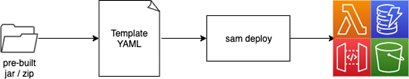
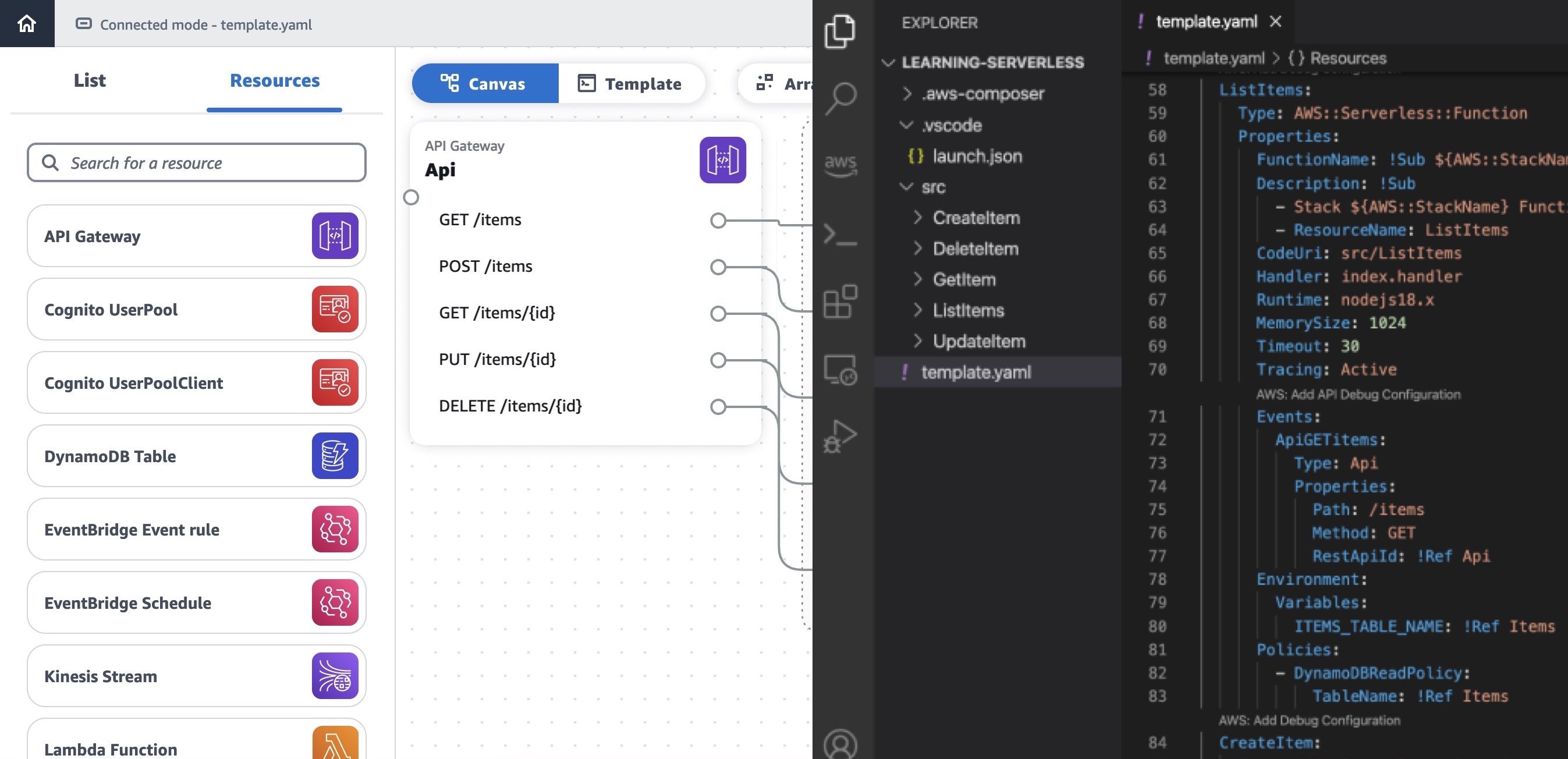
The following diagram provides an overview of the build and deployment process with AWS SAM CLI. The default behavior includes the following steps:

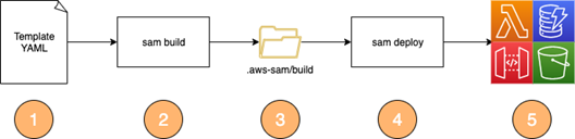
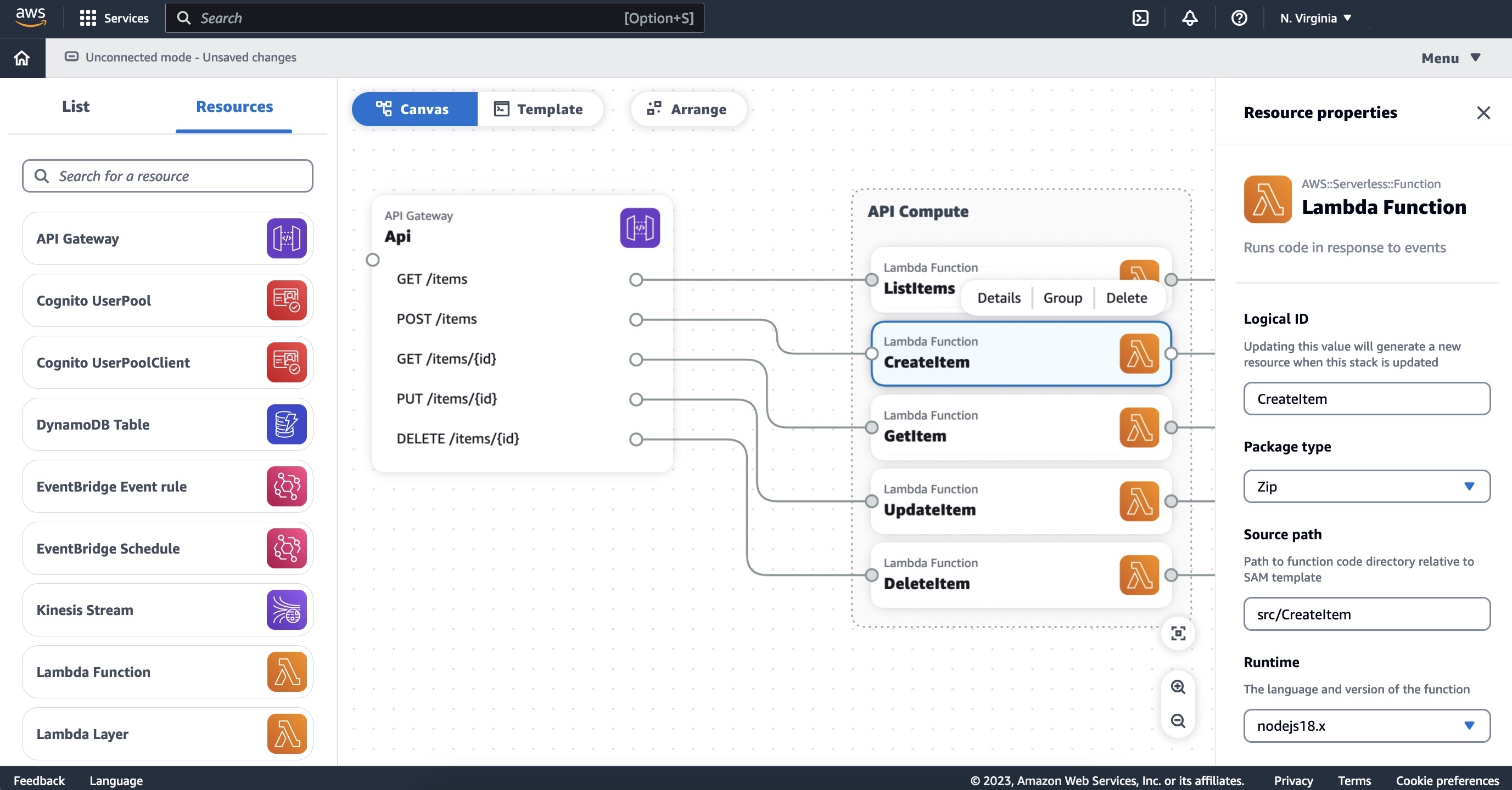
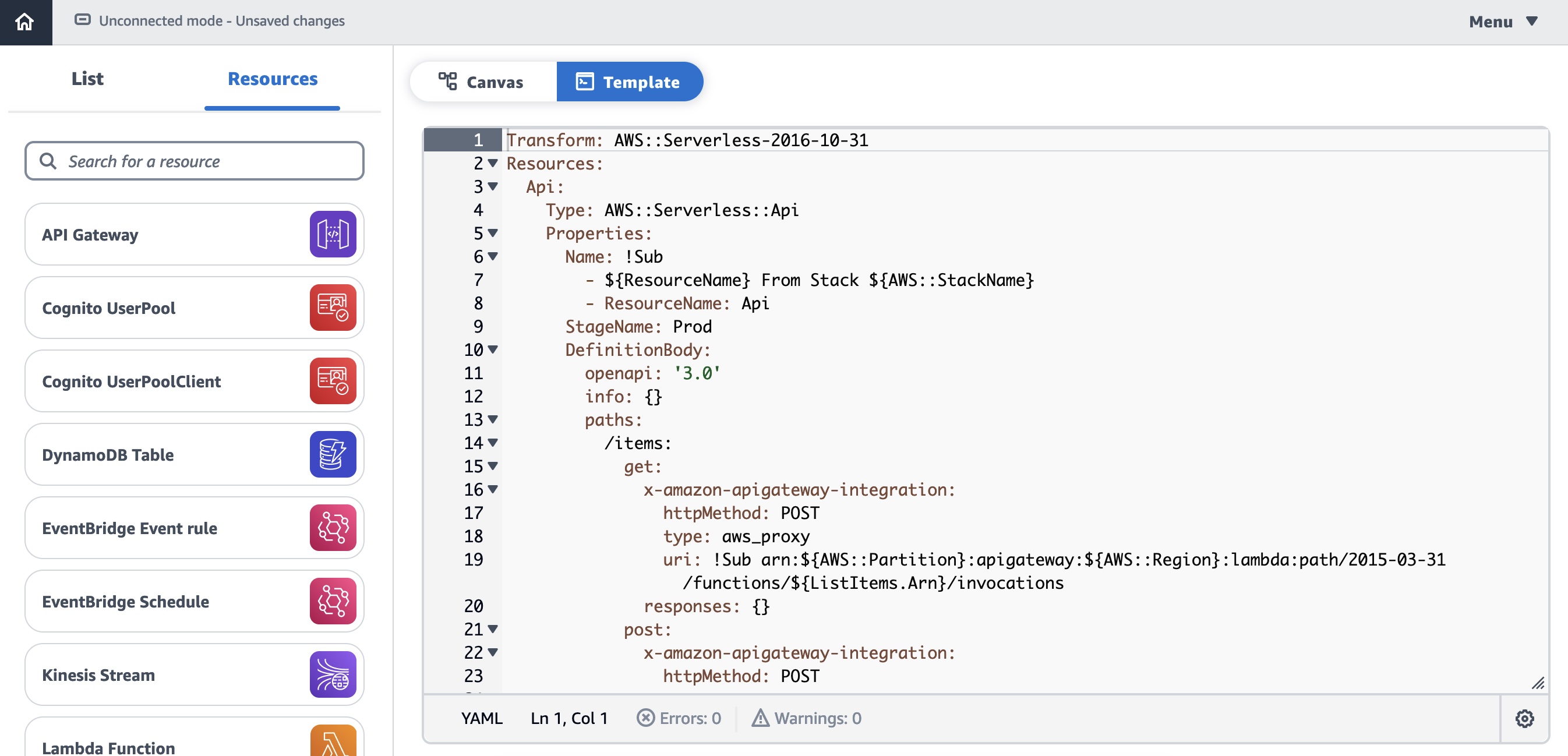
Define your infrastructure resources such as Lambda functions, Amazon DynamoDB Tables, Amazon S3 buckets, or an Amazon API Gateway endpoint in a template.yaml file.
The CLI command “sam build” builds the application based on the chosen runtime and configuration within the template.
The sam build command populates the .aws-sam/build folder with the built artifacts (for example, class files or jars).
The sam deploy command uploads your template and function code from the .aws-sam/build folder and starts an AWS CloudFormation deployment.
After a successful deployment, you can find the provisioned resources in your AWS account.

Using the default Java build mechanism in AWS SAM CLI

AWS SAM CLI supports building Serverless Java functions with Maven or Gradle. You must use one of the supported Java runtimes (java8, java8.al2, java11) and your function’s resource CodeUri property must point to a source folder.

AWS SAM CLI ships with default build mechanisms provided by the aws-lambda-builders project. It is therefore not required to package or build your application in advance and any customized build steps in pom.xml will not be used. For example, by default the AWS SAM Maven Lambda Builder triggers the following steps:

mvn clean install to build the function.
mvn dependency:copy-dependencies -DincludeScope=runtime -Dmdep.prependGroupId=true to prepare dependency jar files.
Class files in target/classes and dependency jar archives in target/dependency are copied to the final build artifact location in .aws-sam/build/{ResourceLogicalId}.

Start the build process by running the following command from the directory where the template.yaml resides:

sam build

This results in the following outputs:

The .aws-sam build folder contains the necessary classes and libraries to run your application. The transformed template.yaml file points to the build artifacts directory (instead of pointing to the original source directory).

Run the following command to deploy the resources to AWS:

sam deploy --guided

This zips the HelloWorldFunction directory in .aws-sam/build and uploads it to the Lambda service.

Building Uber-Jars with AWS SAM CLI

A popular way for building and packaging Java projects, especially when using frameworks such as Micronaut, Quarkus and Spring Boot is to create an Uber-jar or Fat-jar. This is a jar file that contains the application class files with all the dependency class files within a single jar file. This simplifies the deployment and management of the application artifact.

Frameworks typically provide a Maven or Gradle setup that produces an Uber-jar by default. For example, by using the Apache Maven Shade plugin for Maven, you can configure Uber-jar packaging:

<build>
  <plugins>
    <plugin>
      <groupId>org.apache.maven.plugins</groupId>
      <artifactId>maven-shade-plugin</artifactId>
      <version>3.4.1</version>
      <executions>
 	 <execution>
 	   <phase>package</phase>
 	     <goals>
 	       <goal>shade</goal>
 	     </goals>
 	 </execution>
      </executions>
     </plugin>
  </plugins>
</build>

The maven-shade-plugin modifies the package phase of the Maven build to produce the Uber-jar file in the target directory.

To build and package an Uber-jar with AWS SAM, you must customize the AWS SAM CLI build process. You can do this by using a Makefile to replace the default steps discussed earlier. Within the template.yaml, declare a Metadata resource attribute with a BuildMethod entry. The sam build process then looks for a Makefile within the CodeUri directory.

The Makefile is responsible for building the artifacts required by AWS SAM to deploy the Lambda function. AWS SAM runs the target in the Makefile. This is an example Makefile:

build-HelloWorldFunctionUberJar:
 	mvn clean package
 	mkdir -p $(ARTIFACTS_DIR)/lib
 	cp ./target/HelloWorld*.jar $(ARTIFACTS_DIR)/lib/

The Makefile runs the Maven clean and package goals that build Uber-jar in the target directory via the Apache Maven Plugin. As the Lambda Java runtime loads jar files from the lib directory, you can copy the uber-jar file to the $ARTIFACTS_DIR/lib directory as part of the build steps.

To build the application, run:

sam build

This triggers the customized build step and creates the following output resources:

The deployment step is identical to the previous example.

Running the build process inside a container

AWS SAM provides a mechanism to run the application build process inside a Docker container. This provides the benefit of not requiring your build dependencies (such as Maven and Java) to be installed locally or in your CI/CD environment.

To run the build process inside a container, use the command line options –use-container and optionally –build-image. The following diagram outlines the modified build process with this option:

Similar to the previous examples, the directory with the application sources or the Makefile is referenced.
To run the build process inside a Docker container, provide the command line option:
```
sam build –-use-container
```
By default, AWS SAM uses images for container builds that are maintained in the GitHub repo aws/aws-sam-build-images. AWS SAM pulls the container image depending on the defined runtime. For this example, it pulls the public.ecr.aws/sam/build-java11 image, which has prerequisites such as Maven and Java11 pre-installed to build the application. In addition, the source code folder is mounted in the container and the Makefile target or default build mechanism is run within the container.
The final artifacts are delivered to the.aws-sam/build directory on the local file system. If you are using a Makefile, you can copy the final artifact to the $ARTIFACTS_DIR.
The sam deploy command uploads the template and function code from the .aws-sam/build directory and starts a CloudFormation deployment.
After a successful deployment, you can find the provisioned resources in your AWS account.

To test the behavior, run the previous examples with the –use-container option. No additional changes are needed.

Using your own base build images for creating custom runtimes

When you are targeting a non-supported Lambda runtime, such as a non-LTS Java version or natively compiled GraalVM native images, you can create your own build image with the necessary dependencies installed.

For example, to build a native image with GraalVM, you must have GraalVM and the native image tool installed when building your application.

To create a custom image:

Create a Dockerfile with the needed dependencies:

#Use the official AWS SAM base image or Amazon Linux 2 as a starting point
FROM public.ecr.aws/sam/build-java11:latest-x86_64

#Install GraalVM dependencies
ENV GRAAL_VERSION 22.2.0
ENV GRAAL_FOLDERNAME graalvm-ce-java11-${GRAAL_VERSION}
ENV GRAAL_FILENAME graalvm-ce-java11-linux-amd64-${GRAAL_VERSION}.tar.gz
RUN curl -4 -L https://github.com/graalvm/graalvm-ce-builds/releases/download/vm-22.2.0/graalvm-ce-java11-linux-amd64-22.2.0.tar.gz | tar -xvz
RUN mv $GRAAL_FOLDERNAME /usr/lib/graalvm
RUN rm -rf $GRAAL_FOLDERNAME

#Install Native Image dependencies
RUN /usr/lib/graalvm/bin/gu install native-image
RUN ln -s /usr/lib/graalvm/bin/native-image /usr/bin/native-image
RUN ln -s /usr/lib/maven/bin/mvn /usr/bin/mvn

#Set GraalVM as default
ENV JAVA_HOME /usr/lib/graalvm

Build your image locally or upload it to a container registry:
```
docker build . -t sam/custom-graal-image
```
Use AWS SAM build with the build image argument to provide your custom image:
```
sam build --use-container --build-image sam/custom-graal-image
```

You can find the source code and an example Dockerfile, Makefile, and pom.xml for GraalVM native images in the GitHub repo.

When you use the official AWS SAM build images as a base image, you have all the necessary tooling such as Maven, Java11 and the Lambda builders installed. If you want to use a more customized approach and use a different base image, you must install these dependencies.

For an example, check the GraalVM with Java 17 cookiecutter template. In addition, there are multiple additional components involved when building custom runtimes, which are outlined in “Build a custom Java runtime for AWS Lambda”.

To avoid providing the command line options on every build, include them in the samconfig.toml file:

[default.build.parameters]
use_container = true
build_image = ["public.ecr.aws/sam/build-java11:latest-x86_64"]

For additional information, refer to the official AWS SAM CLI documentation.

Deploying the application without building with AWS SAM

There might be scenarios where you do not want to rely on the build process offered by AWS SAM. For example, when you have highly customized or established build processes, or advanced dependency caching or visibility requirements.

In this case, you can still use the AWS SAM CLI commands such as sam local and sam deploy. But you must point your CodeUri property directly to the pre-built artifact (instead of the source code directory):

HelloWorldFunctionSkipBuild:
  Type: AWS::Serverless::Function
  Properties:
    CodeUri: HelloWorldFunction/target/HelloWorld-1.0.jar
    Handler: helloworld.App::handleRequest

In this case, there is no need to use the sam build command, since the build logic is outside of AWS SAM CLI:

Here, the sam build command fails because it looks for a source folder to build the application. However, there might be cases where you have a mixed setup that includes some functions that point to pre-built artifacts and others that are built by AWS SAM CLI. In this scenario, you can mark those functions to explicitly skip the build process by adding the following SkipBuild flag in the Metadata section of your resource definition:

HelloWorldFunctionSkipBuild:
  Type: AWS::Serverless::Function
  Properties:
    CodeUri: HelloWorldFunction/target/HelloWorld-1.0.jar
    Handler: helloworld.App::handleRequest
    Runtime: java11
  Metadata:
    SkipBuild: True

Conclusion

This blog post shows how to build Java applications with the AWS SAM CLI. You learnt about the default build mechanisms, and how to customize the build behavior and abstract the build process inside a container environment. Visit the GitHub repository for the example code templates referenced in the examples.

To learn more, dive deep into the AWS SAM documentation. For more serverless learning resources, visit Serverless Land.

Server-side rendering micro-frontends – UI composer and service discovery

2023-03-09 James Beswick

Post Syndicated from James Beswick original https://aws.amazon.com/blogs/compute/server-side-rendering-micro-frontends-ui-composer-and-service-discovery/

This post is written by Luca Mezzalira, Principal Specialist Solutions Architect, Serverless.

The previous blog post describes the architecture for creating a server-side rendering micro-frontend in AWS. This and subsequent posts explain the different parts that compose this architecture in detail. The code for the example is available on a AWS Samples GitHub repository.

For context, this post covers the infrastructure related to the UI composer, and why you need an Amazon S3 bucket for storing static assets:

The rest of the series explores the micro-frontends composition, how to design micro-frontends using serverless services, different caching and performance optimization strategies, and the organization structure implications associated with frontend distributed systems.

A user’s request journey

The best way to navigate through this distributed system is by simulating a user request that touches all the parts implemented in the architecture.

The application example shows a product details page of a hypothetical ecommerce platform:

When a user selects an article from the catalog page, the DNS resolves the URL to an Amazon CloudFront distribution that is the reference CDN for this project.

The request is immediately fulfilled if the page is cached. Therefore, no additional logic is requested by the cloud infrastructure and the response is fast (less than the 500 ms shown in this example).

When the page is not available in the CloudFront points of presence (PoPs), the request is forwarded to the Application Load Balancer (ALB). It arrives at the AWS Fargate cluster where the UI Composer generates the page for fulfilling the request.

Using CloudFront in the architecture

CDNs are known for accelerating application delivery thanks to caching static files from nearby PoPs. CloudFront can also accelerate uncacheable content such as dynamic APIs or personalized content.

With a network of over 450 points of presence, CloudFront terminates user TCP/TLS connections within 20-30 milliseconds on average. Traffic to origin servers is carried over the AWS global network instead of the public internet. This infrastructure is a purpose-built, highly available, and low-latency private infrastructure built on a global, fully redundant, metro fiber network that is linked via terrestrial and trans-oceanic cables across the world. In addition to terminating connections close to users, CloudFront accelerates dynamic content thanks to modern internet protocols such as QUIC and TLS1.3, and persisting TCP connections to the origin servers.

CloudFront also has security benefits, offering protection in AWS against infrastructure DDoS attacks. It integrates with AWS Web Application Firewall and AWS Shield Advanced, giving you controls to block application-level DDoS attacks. CloudFront also offers native security controls such as HTTP to HTTPS redirections, CORS management, geo-blocking, tokenization, and managing security response headers.

UI Composer application logic

When the request is not fulfilled by the CloudFront cache, it is routed to the Fargate cluster. Here, multiple tasks compute and serve the page requested.

This example uses Fastify, a fast Node.js framework that is gaining popularity among the Node.js community. When the web server initializes, it loads external parameters and the template for composing a page.

const start = async () => {
  try {
    //load parameters
    MFElist = await init();
    //load catalog template
    catalogTemplate = await loadFromS3(MFElist.template, MFElist.templatesBucket)
    await fastify.listen({ port: PORT, host: '0.0.0.0' })
  } catch (err) {
    fastify.log.error(err)
    process.exit(1)
  }
}

To maintain team independence and avoid redeploying the UI composer for every application change, the HTML templates are loaded from an S3 bucket. All teams responsible for micro-frontends in the same page can position their micro-frontends into the right place of the HTML template and delegate the composition task to the UI composer.

In this demo, the initial parameters and the catalog template are retrieved once. However, in a real scenario, it’s more likely you retrieve the parameters at initialization and at a regular cadence. The template might be loaded at runtime for every request or have another background routine fetching the initialization parameters in a similar way.

When the request reaches the product details route, the web application logic calls a transformTemplate function. It passes the catalog template, retrieved from the S3 bucket at the server initialization. It returns a 200 response if the page is composed without any issues.

fastify.get('/productdetails', async(request, reply) => {
  try{
    const catalogDetailspage = await transformTemplate(catalogTemplate)
    responseStream(catalogDetailspage, 200, reply)
  } catch(err){
    console.log(err)
    throw new Error(err)
  }
})

The page composition is the key responsibility of the UI composer. There are several viable approaches for composing micro-frontends in a server-side rendering system, covered in the next post.

Micro-frontends discovery

To decouple workloads for multiple teams, you must use architectural patterns that support it. In a microservices architecture, a pattern that allows independent evolution of a service without coupling the DNS or IP to any microservice is the service discovery pattern.

In this example, AWS System Managers Parameters Store acts as a services registry. Every micro-frontend available in the workload registers itself once the infrastructure is provisioned.

In this way, the UI composer can request the micro-frontend ID found inside the HTML template. It can retrieve the correct way to consume the micro-frontend API using an ARN or a remote HTTP URL, for instance.

Using ARN over HTTP requests inside the workload network can help you to reduce the latency thanks to fewer network hops. Moreover, the security is delegated to IAM policies providing a robust security implementation.

The UI composer takes care to retrieve the micro-frontends endpoints at runtime before loading them into the HTML template. This is a simpler yet powerful approach for maintaining the boundaries within your organization and allowing independent teams to evolve their architecture autonomously.

Micro-frontends discovery evolution

Using Parameter Store as a service discovery system, you can deploy a new micro-frontend by adding a new key-value into the service discovery.

A more sophisticated option could be creating a service that acts as a registry and also shapes the traffic towards different micro-frontends versions using deployment strategies like canary releases or blue/green deployments.

You can start iteratively with a simple key-value store system and evolve the architecture with a more complex approach when the workload requires, providing a robust way to roll out micro-frontends services in your system.

When this is in place, it’s likely to increase the release cadence of your micro-frontends. This is because developers often feel safer releasing in production without affecting the entire user base and they can run tests alongside real traffic.

Performance considerations

This architecture uses Fargate for composing the micro-frontends instead of Lambda functions. This allows incremental rendering offered by browsers, displaying the HTML page partially before it’s completely returned.

Consider a scenario where a micro-frontend takes longer to render due to a downstream dependency or a faulty version deployed into production. Without the streaming capability, you must wait until all the micro-frontends responses arrive, buffer them in memory, compose the page and then send the final output to the browser.

Instead, by using the streaming API offered by Node.js frameworks, you can send a partial HTML page (for example, the head tag and subsequently the rest of the page), to be rendered by a browser.

Streaming also improves server overhead, because the servers don’t have to buffer entire pages. By incrementally flushing data to browsers, servers keep memory pressure low, which lets them process more requests and save overhead costs.

However, in case your workload doesn’t require these capabilities, one or multiple Lambda functions might be suitable for your project as well, reducing the infrastructure management complexity to handle.

Conclusion

This post looks at how to use the UI Composer and micro-frontends discoverability. Once this part is developed, it won’t need to change regularly. This represents the foundation for building server-side rendering micro-frontends using HTML-over-the-wire. There might be other approaches to follow for other frameworks such as Next.js due to the architectural implementation of the framework itself.

The next post will cover how the UI composer includes micro-frontends output inside an HTML template.

For more serverless learning resources, visit Serverless Land.

How gaming companies can use Amazon Redshift Serverless to build scalable analytical applications faster and easier

2023-03-07 Satesh Sonti

Post Syndicated from Satesh Sonti original https://aws.amazon.com/blogs/big-data/how-gaming-companies-can-use-amazon-redshift-serverless-to-build-scalable-analytical-applications-faster-and-easier/

This post provides guidance on how to build scalable analytical solutions for gaming industry use cases using Amazon Redshift Serverless. It covers how to use a conceptual, logical architecture for some of the most popular gaming industry use cases like event analysis, in-game purchase recommendations, measuring player satisfaction, telemetry data analysis, and more. This post also discusses the art of the possible with newer innovations in AWS services around streaming, machine learning (ML), data sharing, and serverless capabilities.

Our gaming customers tell us that their key business objectives include the following:

Increased revenue from in-app purchases
High average revenue per user and lifetime value
Improved stickiness with better gaming experience
Improved event productivity and high ROI

Our gaming customers also tell us that while building analytics solutions, they want the following:

Low-code or no-code model – Out-of-the-box solutions are preferred to building customized solutions.
Decoupled and scalable – Serverless, auto scaled, and fully managed services are preferred over manually managed services. Each service should be easily replaceable, enhanced with little or no dependency. Solutions should be flexible to scale up and down.
Portability to multiple channels – Solutions should be compatible with most of endpoint channels like PC, mobile, and gaming platforms.
Flexible and easy to use – The solutions should provide less restrictive, easy-to-access, and ready-to-use data. They should also provide optimal performance with low or no tuning.

Analytics reference architecture for gaming organizations

In this section, we discuss how gaming organizations can use a data hub architecture to address the analytical needs of an enterprise, which requires the same data at multiple levels of granularity and different formats, and is standardized for faster consumption. A data hub is a center of data exchange that constitutes a hub of data repositories and is supported by data engineering, data governance, security, and monitoring services.

A data hub contains data at multiple levels of granularity and is often not integrated. It differs from a data lake by offering data that is pre-validated and standardized, allowing for simpler consumption by users. Data hubs and data lakes can coexist in an organization, complementing each other. Data hubs are more focused around enabling businesses to consume standardized data quickly and easily. Data lakes are more focused around storing and maintaining all the data in an organization in one place. And unlike data warehouses, which are primarily analytical stores, a data hub is a combination of all types of repositories—analytical, transactional, operational, reference, and data I/O services, along with governance processes. A data warehouse is one of the components in a data hub.

The following diagram is a conceptual analytics data hub reference architecture. This architecture resembles a hub-and-spoke approach. Data repositories represent the hub. External processes are the spokes feeding data to and from the hub. This reference architecture partly combines a data hub and data lake to enable comprehensive analytics services.

Let’s look at the components of the architecture in more detail.

Sources

Data can be loaded from multiple sources, such as systems of record, data generated from applications, operational data stores, enterprise-wide reference data and metadata, data from vendors and partners, machine-generated data, social sources, and web sources. The source data is usually in either structured or semi-structured formats, which are highly and loosely formatted, respectively.

Data inbound

This section consists of components to process and load the data from multiple sources into data repositories. It can be in batch mode, continuous, pub/sub, or any other
custom integration. ETL (extract, transform, and load) technologies, streaming services, APIs, and data exchange interfaces are the core components of this pillar. Unlike ingestion processes, data can be transformed as per business rules before loading. You can apply technical or business data quality rules and load raw data as well. Essentially, it provides the flexibility to get the data into repositories in its most usable form.

Data repositories

This section consists of a group of data stores, which includes data warehouses, transactional or operational data stores, reference data stores, domain data stores housing purpose-built business views, and enterprise datasets (file storage). The file storage component is usually a common component between a data hub and a data lake to avoid data duplication and provide comprehensiveness. Data can also be shared among all these repositories without physically moving with features, such as data sharing and federated queries. However, data copy and duplication are allowed considering various consumption needs in terms of formats and latency.

Data outbound

Data is often consumed using structured queries for analytical needs. Also, datasets are accessed for ML, data exporting, and publishing needs. This section consists of components to query the data, export, exchange, and APIs. In terms of implementation, the same technologies may be used for both inbound and outbound, but the functions are different. However, it’s not mandatory to use the same technologies. These processes aren’t transformation heavy because the data is already standardized and almost ready to consume. The focus is on the ease of consumption and integration with consuming services.

Consumption

This pillar consists of various consumption channels for enterprise analytical needs. It includes business intelligence (BI) users, canned and interactive reports, dashboards, data science workloads, Internet of Things (IoT), web apps, and third-party data consumers. Popular consumption entities in many organizations are queries, reports, and data science workloads. Because there are multiple data stores maintaining data at different granularity and formats to service consumer needs, these consumption components depend on data catalogs for finding the right source.

Data governance

Data governance is key to the success of a data hub reference architecture. It constitutes components like metadata management, data quality, lineage, masking, and stewardship, which are required for organized maintenance of the data hub. Metadata management helps organize the technical and business metadata catalog, and consumers can reference this catalog to know what data is available in which repository and at what granularity, format, owners, refresh frequency, and so on. Along with metadata management, data quality is important to increase confidence for consumers. This includes data cleansing, validation, conformance, and data controls.

Security and monitoring

Users and application access should be controlled at multiple levels. It starts with authentication, then authorizing who and what should be accessed, policy management, encryption, and applying data compliance rules. It also includes monitoring components to log the activity for auditing and analysis.

Analytics data hub solution architecture on AWS

The following reference architecture provides an AWS stack for the solution components.

Let’s look at each component again and the relevant AWS services.

Data inbound services

AWS Glue and Amazon EMR services are ideal for batch processing. They scale automatically and are able to process most of the industry standard data formats. Amazon Kinesis Data Streams, Amazon Kinesis Data Firehose, and Amazon Managed Streaming for Apache Kafka (Amazon MSK) enables you to build streaming process applications. These streaming services integrate well with the Amazon Redshift streaming feature. This helps you process real-time sources, IoT data, and data from online channels. You can also ingest data with third-party tools like Informatica, dbt, and Matallion.

You can build RESTful APIs and WebSocket APIs using Amazon API Gateway and AWS Lambda, which will enable real-time two-way communication with web sources, social, and IoT sources. AWS Data Exchange helps with subscribing to third-party data in AWS Marketplace. Data subscription and access is fully managed with this service. Refer to the respective service documentation for further details.

Data repository services

Amazon Redshift is the recommended data storage service for OLAP (Online Analytical Processing) workloads such as cloud data warehouses, data marts, and other analytical data stores. This service is the core of this reference architecture on AWS and can address most analytical needs out of the box. You can use simple SQL to analyze structured and semi-structured data across data warehouses, data marts, operational databases, and data lakes to deliver the best price performance at any scale. The Amazon Redshift data sharing feature provides instant, granular, and high-performance access without data copies and data movement across multiple Amazon Redshift data warehouses in the same or different AWS accounts, and across Regions.

For ease of use, Amazon Redshift offers a serverless option. Amazon Redshift Serverless automatically provisions and intelligently scales data warehouse capacity to deliver fast performance for even the most demanding and unpredictable workloads, and you pay only for what you use. Just load your data and start querying right away in Amazon Redshift Query Editor or in your favorite BI tool and continue to enjoy the best price performance and familiar SQL features in an easy-to-use, zero administration environment.

Amazon Relational Database Service (Amazon RDS) is a fully managed service for building transactional and operational data stores. You can choose from many popular engines such as MySQL, PostgreSQL, MariaDB, Oracle, and SQL Server. With the Amazon Redshift federated query feature, you can query transactional and operational data in place without moving the data. The federated query feature currently supports Amazon RDS for PostgreSQL, Amazon Aurora PostgreSQL-Compatible Edition, Amazon RDS for MySQL, and Amazon Aurora MySQL-Compatible Edition.

Amazon Simple Storage Service (Amazon S3) is the recommended service for multi-format storage layers in the architecture. It offers industry-leading scalability, data availability, security, and performance. Organizations typically store data in Amazon S3 using open file formats. Open file formats enable analysis of the same Amazon S3 data using multiple processing and consumption layer components. Data in Amazon S3 can be easily queried in place using SQL with Amazon Redshift Spectrum. It helps you query and retrieve structured and semi-structured data from files in Amazon S3 without having to load the data. Multiple Amazon Redshift data warehouses can concurrently query the same datasets in Amazon S3 without the need to make copies of the data for each data warehouse.

Data outbound services

Amazon Redshift comes with the web-based analytics workbench Query Editor V2.0, which helps you run queries, explore data, create SQL notebooks, and collaborate on data with your teams in SQL through a common interface. AWS Transfer Family helps securely transfer files using SFTP, FTPS, FTP, and AS2 protocols. It supports thousands of concurrent users and is a fully managed, low-code service. Similar to inbound processes, you can utilize Amazon API Gateway and AWS Lambda for data pull using the Amazon Redshift Data API. And AWS Data Exchange helps publish your data to third parties for consumption through AWS Marketplace.

Consumption services

Amazon QuickSight is the recommended service for creating reports and dashboards. It enables you to create interactive dashboards, visualizations, and advanced analytics with ML insights. Amazon SageMaker is the ML platform for all your data science workload needs. It helps you build, train, and deploy models consuming the data from repositories in the data hub. You can use Amazon front-end web and mobile services and AWS IoT services to build web, mobile, and IoT endpoint applications to consume data out of the data hub.

Data governance services

The AWS Glue Data Catalog and AWS Lake Formation are the core data governance services AWS currently offers. These services help manage metadata centrally for all the data repositories and manage access controls. They also help with data classification and can automatically handle schema changes. You can use Amazon DataZone to discover and share data at scale across organizational boundaries with built-in governance and access controls. AWS is investing in this space to provide more a unified experience for AWS services. There are many partner products such as Collibra, Alation, Amorphic, Informatica, and more, which you can use as well for data governance functions with AWS services.

Security and monitoring services

AWS Identity and Access Management (AWS IAM) manages identities for AWS services and resources. You can define users, groups, roles, and policies for fine-grained access management of your workforce and workloads. AWS Key Management Service (AWS KMS) manages AWS keys or customer managed keys for your applications. Amazon CloudWatch and AWS CloudTrail help provide monitoring and auditing capabilities. You can collect metrics and events and analyze them for operational efficiency.

In this post, we’ve discussed the most common AWS services for the respective solution components. However, you aren’t limited to only these services. There are many other AWS services for specific use cases that may be more appropriate for your needs than what we discussed here. You can reach to AWS Analytics Solutions Architects for appropriate guidance.

Example architectures for gaming use cases

In this section, we discuss example architectures for two gaming use cases.

Game event analysis

In-game events (also called timed or live events) encourage player engagement through excitement and anticipation. Events entice players to interact with the game, increasing player satisfaction and revenue with in-game purchases. Events have become more and more important, especially as games shift from being static pieces of entertainment to be played as is to offering dynamic and changing content through the use of services that use information to make decisions about game play as the game is being played. This enables games to change as the players play and influence what works and what doesn’t, and gives any game a potentially infinite lifespan.

This capability of in-game events to offer fresh content and activities within a familiar framework is how you keep players engaged and playing for months to years. Players can enjoy new experiences and challenges within the familiar framework or world that they have grown to love.

The following example shows how such an architecture might appear, including changes to support various sections of the process like breaking the data into separate containers to accommodate scalability, charge-back, and ownership.

To fully understand how events are viewed by the players and to make decisions about future events requires information on how the latest event was actually performed. This means gathering a lot of data as the players play to build key performance indicators (KPIs) that measure the effectiveness and player satisfaction with each event. This requires analytics that specifically measure each event and capture, analyze, report on, and measure player experience for each event. These KPIs include the following:

Initial user flow interactions – What actions users are taking after they first receive or download an event update in a game. Are there any clear drop-off points or bottlenecks that are turning people off the event?
Monetization – When, what, and where users are spending money on in the event, whether it’s buying in-game currencies, answering ads, specials, and so on.
Game economy – How can users earn and spend virtual currencies or goods during an event, using in-game money, trades, or barter.
In-game activity – Player wins, losses, leveling up, competition wins, or player achievements within the event.
User to user interactions – Invitations, gifting, chats (private and group), challenges, and so on during an event.

These are just some of the KPIs and metrics that are key for predictive modeling of events as the game acquires new players while keeping existing users involved, engaged, and playing.

In-game activity analysis

In-game activity analysis essentially looks at any meaningful, purposeful activity the player might show, with the goal of trying to understand what actions are taken, their timing, and outcomes. This includes situational information about the players, including where they are playing (both geographical and cultural), how often, how long, what they undertake on each login, and other activities.

The following example shows how such an architecture might appear, including changes to support various sections of the process like breaking the data into separate warehouses. The multi-cluster warehouse approach helps scale the workload independently, provides flexibility to the implemented charge-back model, and supports decentralized data ownership.

The solution essentially logs information to help understand the behavior of your players, which can lead to insights that increase retention of existing players, and acquisition of new ones. This can provide the ability to do the following:

Provide in-game purchase recommendations
Measure player trends in the short term and over time
Plan events the players will engage in
Understand what parts of your game are most successful and which are less so

You can use this understanding to make decisions about future game updates, make in-game purchase recommendations, determine when and how your game economy may need to be balanced, and even allow players to change their character or play as the game progresses by injecting this information and accompanying decisions back into the game.

Conclusion

This reference architecture, while showing examples of only a few analysis types, provides a faster technology path for enabling game analytics applications. The decoupled, hub/spoke approach brings the agility and flexibility to implement different approaches to analytics and understanding the performance of game applications. The purpose-built AWS services described in this architecture provide comprehensive capabilities to easily collect, store, measure, analyze, and report game and event metrics. This helps you efficiently perform in-game analytics, event analysis, measure player satisfaction, and provide tailor-made recommendations to game players, efficiently organize events, and increase retention rates.

Thanks for reading the post. If you have any feedback or questions, please leave them in the comments.

About the authors

Satesh Sonti is a Sr. Analytics Specialist Solutions Architect based out of Atlanta, specialized in building enterprise data platforms, data warehousing, and analytics solutions. He has over 16 years of experience in building data assets and leading complex data platform programs for banking and insurance clients across the globe.

Tanya Rhodes is a Senior Solutions Architect based out of San Francisco, focused on games customers with emphasis on analytics, scaling, and performance enhancement of games and supporting systems. She has over 25 years of experience in enterprise and solutions architecture specializing in very large business organizations across multiple lines of business including games, banking, healthcare, higher education, and state governments.

AWS Application Composer Now Generally Available – Visually Build Serverless Applications Quickly

2023-03-07 Channy Yun

Post Syndicated from Channy Yun original https://aws.amazon.com/blogs/aws/aws-application-composer-now-generally-available-visually-build-serverless-applications-quickly/

At AWS re:Invent 2022, we previewed AWS Application Composer, a visual builder for you to compose and configure serverless applications from AWS services backed by deployment-ready infrastructure as code (IaC).

In the keynote, Dr. Werner Vogels, CTO of Amazon.com said:

Developers that never used serverless before. How do they know where to start? Which services do they need? How do they work together? We really wanted to make this easier. AWS Application Composer simplifies and accelerates the architecting, configuring, and building of serverless applications.

During the preview, we had lots of interest and great feedback from customers. Today, I am happy to announce the general availability of AWS Application Composer with new improvements based on customer feedback. I want to quickly review its features and introduce some improvements.

Introduction to AWS Application Composer
To get started with AWS Application Composer, choose Open demo in the AWS Management Console. This demo shows a simple cart application with Amazon API Gateway, AWS Lambda, and Amazon DynamoDB resources.

You can easily browse and search for AWS services in the left Resources panel and drag and drop them onto the canvas to expand your architecture.

In the middle Canvas panel, you can connect resources together by clicking and dragging from one resource port to another. Permissions are automatically composed for these resources to interact with each other using policy template, environment variables, and event subscriptions. Grouping resources is very useful to select one visual organization. For above example, API Compute group is compsite of Lambda functions. When you double-click on a specific resource, you can name and configure your properties in the right Resource properties panel.

As well as featured resources available in the visual resource palette, you can use hidden and read-only resources will populate on the canvas when you load an existing template that includes them.

In this example, the MyHttpApi resource is a hidden resource. It is not available from the resource palette but does appear on the canvas in color. The resource named MyHttpApiRole (in this case, an AWS::IAM::Role resource) is read-only. It grayed out on the canvas greyed out. To learn more about all supported resources, see AWS Application Composer featured resources in the AWS documentation.

When you select the Template menu, you can view, edit or manually download your IaC, such as AWS Serverless Application Model (AWS SAM). Your changes are automatically synced with your canvas.

When you start Connected mode, you can use Application Composer with local tools such as an integrated development environment (IDE). Any changes activate the automatic synchronization of your project template and files between Application Composer and your local project directory.

It is useful to incorporate into your existing team processes, such as local testing with AWS SAM Command Line Interface (CLI), peer review through version control, or deployment through AWS CloudFormation and continuous integration and delivery (CI/CD) pipelines.

This mode is supported on Chrome and Edge browsers and requires you to grant temporary local file system access to your browser.

AWS Application Composer can be used in real-world scenarios such as:

Building a prototype of serverless applications
Reviewing and collaboratively evolving existing serverless projects
Generating diagrams for documentation or Wikis
Onboarding new team members to a project
Reducing the first steps to deploy something in an AWS account

To learn more real-world examples, see Visualize and create your serverless workloads with AWS Application Composer in the AWS Compute Blog, How I Used AWS Application Composer to Make Analyzing My Meetup Data Easy in BuildOn.AWS, or watch a breakout session video (SVS211) from AWS re:Invent 2022.

Improvements Since Preview Launch
Here is a new feature to improve how you work with Amazon Simple Queue Service (Amazon SQS) queues.

You can now directly connect Amazon API Gateway resources to Amazon SQS without routing requests through AWS Lambda function. You can remove the complexity of the Lambda function’s execution and increase the reliability while reducing lines of code.

For example, you can drag API Gateway and Amazon SQS onto the canvas and connect the two resources. When the user drags the connector from API route to SQS, Send message appears. You can connect the API route to the SQS queue via their choice of integration target.

The new Change Inspector provides a visual diff of template changes made when you connect two resources on the canvas. This information is available as a notification when you make the connection, which helps you understand how Composer manages integration configuration in your IaC template as you build.

Here are some more improvements to your experience in the user interface!

First, we reduced the size of resource cards. The larger cards made it difficult for the users to read and view their template on the canvas. Now, you can arrange more resource cards easily and save space on the canvas.

Also, we added zoom in and out and zoom to fit buttons so that users can quickly view the entire screen or zoom to the desired level. When you load a large template onto the canvas, you can easily see all the resource cards in any size.

Now Available
AWS Application Composer is now generally available in the US East (Ohio), US East (N. Virginia), US West (Oregon), Asia Pacific (Singapore), Asia Pacific (Sydney), Asia Pacific (Tokyo), Europe (Frankfurt), Europe (Ireland), and Europe (Stockholm) Regions, adding three more Regions to the six Regions available during preview. There is no additional cost, and you can start using it today.

To learn more, see the AWS Application Composer Developer Guide and send feedback to AWS re:Post for AWS Application Composer or through your usual AWS support contacts.

– Channy

Access Amazon Athena in your applications using the WebSocket API

2023-03-03 Abhi Sodhani

Post Syndicated from Abhi Sodhani original https://aws.amazon.com/blogs/big-data/access-amazon-athena-in-your-applications-using-the-websocket-api/

Modern applications are built with modular independent components or microservices that rely on an API framework to communicate with services. Many organizations are building data lakes to store and analyze large volumes of structured, semi-structured, and unstructured data. In addition, many teams are moving towards a data mesh architecture, which requires them to expose their data sets as easily consumable data products. To accomplish this on AWS, organizations use Amazon Simple Storage Service (Amazon S3) to provide cheap and reliable object storage to house their datasets. To enable interactive querying and analyzing their data in place using familiar SQL syntax, many teams are turning to Amazon Athena. Athena is an interactive query service that is used by modern applications to query large volumes of data on an S3 data lake using standard SQL.

When working with SQL databases, application developers and business analysts are most familiar with simple permissions management and synchronous query-response protocols—if a user has permissions to submit a query, they do so and receive the results from the server when the query is complete. Directly accessing Athena APIs, for example when integrating with a custom web application, requires an AWS Identity and Access Management (IAM) role for the applications, and requires you to build a custom process to poll for query completion asynchronously. The IAM role needs access to run Athena API calls, as well as S3 permissions to retrieve the Athena output stored on Amazon S3. Polling for Athena query completion when performed at several intervals could result in increased latency from the client perspective.

In this post, we present a solution that can integrate with your front-end application to query data from Amazon S3 using an Athena synchronous API invocation. With this solution, you can add a layer of abstraction to your application on direct Athena API calls and promote the access using the WebSocket API developed with Amazon API Gateway. The query results are returned back to the application as Amazon S3 presigned URLs.

Overview of solution

For illustration purposes, this post builds a COVID-19 data lake with a WebSocket API to handle Athena queries. Your application can invoke the WebSocket API to pull the data from Amazon S3 using an Athena SQL query, and the WebSocket API returns the JSON response with the presigned Amazon S3 URL. The application needs to parse the JSON message to read the presigned URL, download the data to local, and report the data back to the front end.

We use AWS Step Functions to poll the Athena query run. When the query is complete, Step Functions invokes an AWS Lambda function to generate the presigned URL and send the request back to the application.

The application doesn’t require direct access to Athena, just access to invoke the API. When using this solution, you should secure the API following AWS guidelines. For more information, refer to Controlling and managing access to a WebSocket API in API Gateway.

The following diagram summarizes the architecture, key components, and interactions in the solution.

Architecture diagram for the Athena WebSocket API. The user connects to the API through API Gateway. API Gateway uses Lambda and DynamoDB to store session data. SQL queries are routed to Amazon Athena and a Step Function polls for query status and returns the results back to the user.

The application is composed of the WebSocket API in API Gateway, which handles the connectivity between the client and Athena. A client application using the framework can submit the Athena SQL query and get back the presigned URL containing the query results data. The workflow includes the following steps:

The application invokes the WebSocket API connection.
A Lambda function is invoked to initiate the connection. The connection ID is stored in an Amazon DynamoDB
When the client application is connected, it can invoke the runquery action, which invokes the RunQuery Lambda function.
The function first runs the Athena query.
When the query is started, the function checks the status and uses Step Functions to track the query progress.
Step Functions invokes the third Lambda function to read the processed Athena results and get the presigned S3 URL. Failed messages are routed to an Amazon Simple Notification Service (Amazon SNS) topic, which you can subscribe to.
The presigned URL is returned to the client application.
The connection is closed using the OnDisconnect function.

The RunQuery Lambda function runs the Athena query using the start_query_execution request:

def run_query(client, query):
    """This function executes and sends the query request to Athena."""
    response = client.start_query_execution(
        QueryString=query,
        QueryExecutionContext={
            'Database': params['Database']
        },
        ResultConfiguration={
            'OutputLocation': f's3://{params["BucketName"]}/{params["OutputDir"]}/'
        },
        WorkGroup=params["WorkGroup"]
    )
    return response

The Amazon S3 presigned URL is generated by invoking the generate_presigned_url request with the bucket and key information that hosts the Athena results. The code hard codes the presigner expiration to 120 seconds, which is configurable in the function input parameter PreSignerExpireSeconds. See the following code:

def signed_get_url(event):
    s3 = boto3.client('s3', region_name=params['Region'], config=Config(signature_version='s3v4'))
    # User provided body with object info
    bodyData = json.loads(event['body'])
    try:
        url = s3.generate_presigned_url(
            ClientMethod='get_object',
            Params={
                'Bucket': params['BucketName'],
                'Key': bodyData["ObjectName"]
            },
            ExpiresIn=int(params['PreSignerExpireSeconds'])
        )
        body = {'PreSignedUrl': url, 'ExpiresIn': params['PreSignerExpireSeconds']}
        response = {
            'statusCode': 200,
			'body': json.dumps(body),
            'headers': cors.global_returns["Allow Origin Header"]
        }
        logger.info(f"[MESSAGE] Response for PreSignedURL: {response}")
    except Exception as e:
        logger.exception(f"[MESSAGE] Unable to generate URL: {str(e)}")
        response = {
            'statusCode': 502,
            'body': 'Unable to generate PreSignedUrl',
            'headers': cors.global_returns["Allow Origin Header"]
        }
    return response

Prerequisites

This post assumes you have the following:

Access to an AWS account
Permissions to create an AWS CloudFormation stack
Permissions to create the following resources:
- AWS Glue catalog databases and tables
- API Gateway
- Lambda function
- IAM roles
- Step Functions state machine
- SNS topic
- DynamoDB table

Enable the WebSocket API

To enable the WebSocket API of API Gateway, complete the following steps:

Configure the Athena dataset.

To make the data from the AWS COVID-19 data lake available in the Data Catalog in your AWS account, create a CloudFormation stack using the following template. If you’re signed in to your AWS account, the following page fills out most of the stack creation form for you. All you need to do is choose Create stack. For instructions on creating a CloudFormation stack, see Getting started with AWS CloudFormation.

You can also use an existing Athena database to query, in which case you need to update the stack parameters.

If this is the first time you’re using Athena, you must specify a query result location on Amazon S3. For more information about querying and accessing the data from Athena, see A public data lake for analysis of COVID-19 data.

Configure the WebSocket framework using the following page, which deploys the API infrastructure using AWS Serverless Application Model (AWS SAM).
Update the parameters pBucketName with the S3 bucket (in the us-east-2 region) that stores the Athena results and also update the database if you want to query an existing database.
Select the check box to acknowledge creation of IAM roles and choose Deploy.

At a high level, these are the primary resources deployed by the application template:

An API Gateway with routes to the connect, disconnect, and query Lambda functions. Note that the API Gateway deployed with this sample doesn’t implement authentication and authorization. We recommend that you implement authentication and authorization before deploying into a production environment. Refer to Controlling and managing access to a WebSocket API in API Gateway to understand how to implement these security controls.
A DynamoDB table for tracking client connections.
Lambda functions to manage connection states using DynamoDB.
A Lambda function to run the query and start the step function. The function includes an associated IAM role and policies with permissions to Step Functions, the AWS Glue Data Catalog, Athena, AWS Key Management Service (AWS KMS), and Amazon S3. Note that the Lambda execution role gives read access to the Data Catalog and S3 bucket that you specify in the deployment parameters. We recommend that you don’t include a catalog that contains sensitive data without first understanding the impacts and implementing additional security controls.
A Lambda function with associated permissions to poll for the query results and return the presigned URL to the client.
A Step Functions state machine with associated permissions to run the polling Lambda function and send API notifications using Amazon SNS.

Test the setup

To test the WebSocket API, you can use wscat, an open-source command line tool.

Install NPM.
Install wscat:

$ npm install -g wscat

On the console, connect to your published API endpoint by running the following command. The full URI to use can be found on the AWS CloudFormation console by finding the WebSocketURI output in the serverlessrepo-aws-app-athena-websocket-integration stack that was deployed by the AWS SAM application you deployed previously.

$ wscat -c wss://{YOUR-API-ID}.execute-api.{YOUR-REGION}.amazonaws.com/{STAGE}

To test the runquery function, send a JSON message like the following example. This triggers the state machine to run your SQL query using Athena and, using Lambda, return an S3 presigned URL to your client, which you can access to download the query results. Note that the API accepts any valid Athena query. Additional query validation could be added to the internal Lambda function if desired.

$ wscat -c wss://{YOUR-API-ID}.execute-api.{YOUR-REGION}.amazonaws.com/{STAGE}
Connected (press CTRL+C to quit)
> {"action":"runquery", "data":"SELECT * FROM \"covid-19\".country_codes limit 5"}
< {"pre-signed-url": "https://xxx-s3.amazonaws.com/athena_api_access_results/xxxxx.csv?"}

Copy the value for pre-signed-url and enter it into your browser window to access the results.

The presigned URL provides you temporary credentials to download the query results. For more information, refer to Using presigned URLs. This process can be integrated into a front-end web application to automatically download and display the results of the query.

Clean up

To avoid incurring ongoing charges, delete the resources you provisioned by deleting the CloudFormation stacks CovidLakeStacks and serverlessrepo-AthenaWebSocketIntegration via the AWS CloudFormation console. For detailed instructions, refer to the cleanup sections in the starter kit README files in the GitHub repo.

Conclusion

In this post, we showed how to integrate your application with Athena using the WebSocket API. We have included a GitHub repo for you to understand the code and modify it per your application requirements, to get the full benefits of the solution. We encourage you to further explore the features of the API Gateway WebSocket API to add in security using authorizers, view live invocations using dashboards, and expand the framework for more routes on action request.

Let’s stay in touch via the GitHub repo.

About the Authors

Abhi Sodhani is a Sr. AI/ML Solutions Architect at AWS. He helps customers with a wide range of solutions, including machine leaning, artificial intelligence, data lakes, data warehousing, and data visualization. Outside of work, he is passionate about books, yoga, and travel.

Robin Zimmerman is a Data and ML Engineer with AWS Professional Services. He works with AWS enterprise customers to develop systems to extract value from large volumes of data using AWS data, analytics, and machine learning services. When he’s not working, you’ll probably find him in the mountains—rock climbing, skiing, mountain biking, or out on whatever other adventure he can dream up.

How we built an open-source SEO tool using Workers, D1, and Queues

2023-03-02 Kristian Freeman

Post Syndicated from Kristian Freeman original https://blog.cloudflare.com/how-we-built-an-open-source-seo-tool-using-workers-d1-and-queues/

How we built an open-source SEO tool using Workers, D1, and Queues

Building applications on Cloudflare Workers has always been fun. Workers applications have low latency response times by default, and easy developer ergonomics thanks to Wrangler. It’s no surprise that for years now, developers have been going from idea to production with Workers in just a few minutes.

Internally, we’re no different. When a member of our team has a project idea, we often reach for Workers first, and not just for the MVP stage, but in production, too. Workers have been a secret ingredient to Cloudflare’s innovation for some time now, allowing us to build products like Access, Stream and Workers KV. Even better, when we have new ideas and we can use new Cloudflare products to build them, it’s a great way to give feedback on those products.

We’ve discussed this in the past on the Cloudflare blog – in May last year, I wrote how we rebuilt Cloudflare’s developer documentation using many of the tools that had recently been released in the Workers ecosystem: Cloudflare Pages for hosting, and Bulk Redirects for the redirect rules. In November, we released a new version of our API documentation, which again used Pages for hosting, and Pages functions for intelligent caching and transformation of our API schema.

In this blog post, I’m excited to show off some of the new tools in Cloudflare’s developer arsenal, D1 and Queues, to prototype and ship an internal tool for our SEO experts at Cloudflare. We’ve made this project, which we’re calling Prospector, open-source too – check it out in our cloudflare/templates repo on GitHub. Whether you’re a developer looking to understand how to use multiple parts of Cloudflare’s developer stack together, or an SEO specialist who may want to deploy the tool in production, we’ve made it incredibly easy to get up and running.

What we’re building

Prospector is a tool that allows Cloudflare’s SEO experts to monitor our blog and marketing site for specific keywords. When a keyword is matched on a page, Prospector will notify an email address. This allows our SEO experts to stay informed of any changes to our website, and take action accordingly.

Using MailChannels’ integration with Workers, we can quickly and easily send emails from our application using a single API call. This allows us to focus on the core functionality of the application, and not worry about the details of sending emails.

Prospector uses Cloudflare Workers as the user-facing API for the application. It uses D1 to store and retrieve data in real-time, and Queues to handle the fetching of all URLs and the notification process. We’ve also included an intuitive user interface for the application, which is built with HTML, CSS, and JavaScript.

Why we built it

It is widely known in SEO that both internal and external links help Google and other search engines understand what a website is about, which impacts keyword rankings. Not only do these links guide readers to additional helpful information, they also allow web crawlers for search engines to discover and index content on the site.

Acquiring external links is often a time-consuming process and at the discretion of third parties, whereas website owners typically have much more control over internal links. As a result, internal linking is one of the most useful levers available in SEO.

In an ideal world, every piece of content would be fully formed upon publication, replete with helpful internal links throughout the piece. However, this is often not the case. Many times, content is edited after the fact or additional pieces of relevant content come along after initial publication. These situations result in missed opportunities for internal linking.

Like other large organizations, Cloudflare has published thousands of blogs and web pages over the years. We share new content every time a product/technology is introduced and improved. Ultimately, that also means it’s become more challenging to identify opportunities for internal linking in a timely, automated fashion. We needed a tool that would allow us to identify internal linking opportunities as they appear, and speed up the time it takes to identify new internal linking opportunities.

Although we tested several tools that might solve this problem, we found that they were limited in several ways. First, some tools only scanned the first 2,000 characters of a web page. Any opportunities found beyond that limit would not be detected. Next, some tools did not allow us to limit searches to certain areas of the site and resulted in many false positives. Finally, other potential solutions required manual operation, leaving the process at the mercy of human memory.

To solve our problem (and ultimately, improve our SEO), we needed an automated tool that could discover and notify us of new instances of targeted phrases on a specified range of pages.

How it works

Data model

First, let’s explore the data model for Prospector. We have two main tables: notifiers and urls. The notifiers table stores the email address and keyword that we want to monitor. The urls table stores the URL and sitemap that we want to scrape. The notifiers table has a one-to-many relationship with the urls table, meaning that each notifier can have many URLs associated with it.

In addition, we have a sitemaps table that stores the sitemap URLs that we’ve scraped. Many larger websites don’t just have a single sitemap: the Cloudflare blog, for instance, has a primary sitemap that contains four sub-sitemaps. When the application is deployed, a primary sitemap is provided as configuration, and Prospector will parse it to find all of the sub-sitemaps.

Finally, notifier_matches is a table that stores the matches between a notifier and a URL. This allows us to keep track of which URLs have already been matched, and which ones still need to be processed. When a match has been found, the notifier_matches table is updated to reflect that, and “matches” for a keyword are no longer processed. This saves our SEO experts from a crowded inbox, and allows them to focus and act on new matches.

Connecting the pieces with Cloudflare Queues
Cloudflare Queues acts as the work queue for Prospector. When a new notifier is added, a new job is created for it and added to the queue. Behind the scenes, Queues will distribute the work across multiple Workers, allowing us to scale the application as needed. When a job is processed, Prospector will scrape the URL and check for matches. If a match is found, Prospector will send an email to the notifier’s email address.

Using the Cron Triggers functionality in Workers, we can schedule the scraping process to run at a regular interval – by default, once a day. This allows us to keep our data up-to-date, and ensures that we’re always notified of any changes to our website. It also allows the end-user to configure when they receive emails in case they want to receive them more or less frequently, or at the beginning of their workday.

The Module Workers syntax for Workers makes accessing the application bindings – the constants available in the application for querying D1, Queues, and other services – incredibly easy. src/index.ts, the entrypoint for the application, looks like this:

import { DBUrl, Env } from './types'

import {
  handleQueuedUrl,
  scheduled,
} from './functions';

import h from './api'

export default {
  async fetch(
	request: Request,
	env: Env,
	ctx: ExecutionContext
  ): Promise<Response> {
	return h.fetch(request, env, ctx)
  },

  async queue(
	batch: MessageBatch<Error>,
	env: Env
  ): Promise<void> {
	for (const message of batch.messages) {
  	const url: DBUrl = JSON.parse(message.body)
  	await handleQueuedUrl(url, env.DB)
	}
  },

  async scheduled(
	env: Env,
  ): Promise<void> {
	await scheduled({
  	authToken: env.AUTH_TOKEN,
  	db: env.DB,
  	queue: env.QUEUE,
  	sitemapUrl: env.SITEMAP_URL,
	})
  }
};

With this syntax, we can see where the various events incoming to the application – the fetch event, the queue event, and the scheduled event – are handled. The fetch event is the main entrypoint for the application, and is where we handle all of the API routes. The queue event is where we handle the work that’s been added to the queue, and the scheduled event is where we handle the scheduled scraping process.

Central to the application, of course, is Workers – acting as the API gateway and coordinator. We’ve elected to use the popular open-source framework Hono, an Express-style API for Workers, in Prospector. With Hono, we can quickly map out a REST API in just a few lines of code. Here’s an example of a few API routes and how they’re defined with Hono:

const app = new Hono()

app.get("/", (context) => {
  return context.html(index)
})

app.post("/notifiers", async context => {
  try {
	const { keyword, email } = await context.req.parseBody()
	await context.env.DB.prepare(
  	"insert into notifiers (keyword, email) values (?, ?)"
	).bind(keyword, email).run()
	return context.redirect('/')
  } catch (err) {
	context.status(500)
	return context.text("Something went wrong")
  }
})

app.get('/sitemaps', async (context) => {
  const query = await context.env.DB.prepare(
	"select * from sitemaps"
  ).all();
  const sitemaps: Array<DBSitemap> = query.results
  return context.json(sitemaps)
})

Crucial to the development of Prospector are the improved TypeScript bindings for Workers. As announced in November of last year, TypeScript bindings for Workers are now automatically generated based on our open source runtime, workerd. This means that whenever we use the types provided from the @cloudflare/workers-types package in our application, we can be sure that the types are always up-to-date.

With these bindings, we can define the types for our environment variables, and use them in our application. Here’s an example of the Env type, which defines the environment variables that we use in the application:

export interface Env {
  AUTH_TOKEN: string
  DB: D1Database
  QUEUE: Queue
  SITEMAP_URL: string
}

Notice the types of the DB and QUEUE bindings – D1Database and Queue, respectively. These types are automatically generated, complete with type signatures for each method inside of the D1 and Queue APIs. This means that we can be sure that we’re using the correct methods, and that we’re passing the correct arguments to them, directly from our text editor – without having to refer to the documentation.

How to use it

One of my favorite things about Workers is that deploying applications is quick and easy. Using `wrangler.toml` and some simple build scripts, we can deploy a fully-functional application in just a few minutes. Prospector is no different. With just a few commands, we can create the necessary D1 database and Queues instance, and deploy the application to our account.

First, you’ll need to clone the repository from our cloudflare/templates repository:

git clone $URL

If you haven’t installed wrangler yet, you can do so by running:

npm install @cloudflare/wrangler -g

With Wrangler installed, you can login to your account by running:

wrangler login

After you’ve done that, you’ll need to create a new D1 database, as well as a Queues instance. You can do this by running the following commands:

wrangler d1 create $DATABASE_NAME
wrangler queues create $QUEUE_NAME

Configure your wrangler.toml with the appropriate bindings (see [the README](URL) for an example):

[[ d1_databases ]]
binding = "DB"
database_name = "keyword-tracker-db"
database_id = "ab4828aa-723b-4a77-a3f2-a2e6a21c4f87"
preview_database_id = "8a77a074-8631-48ca-ba41-a00d0206de32"
	
[[queues.producers]]
  queue = "queue"
  binding = "QUEUE"

[[queues.consumers]]
  queue = "queue"
  max_batch_size = 10
  max_batch_timeout = 30
  max_retries = 10
  dead_letter_queue = "queue-dlq"

Next, you can run the bin/migrate script to create the tables in your database:

bin/migrate

This will create all the needed tables in your database, both in development (locally) and in production. Note that you’ll even see the creation of a honest-to-goodness .sqlite3 file in your project directory – this is the local development database, which you can connect to directly using the same SQLite CLI that you’re used to:

$ sqlite3 .wrangler/state/d1/DB.sqlite3
sqlite> .tables notifier_matches notifiers sitemaps urls

Finally, you can deploy the application to your account:

npm run deploy

With a deployed application, you can visit your Workers URL to see the user interface. From there, you can add new notifiers and URLs, and see the results of your scraping process. When a new keyword match is found, you’ll receive an email with the details of the match instantly:

Conclusion

For some time, there have been a great deal of applications that were hard to build on Workers without relational data or background task tooling. Now, with D1 and Queues, we can build applications that seamlessly integrate between real-time user interfaces, geographically distributed data, background processing, and more, all using the same developer ergonomics and low latency that Workers is known for.

D1 has been crucial for building this application. On larger sites, the number of URLs that need to be scraped can be quite large. If we were to use Workers KV, our key-value store, for storing this data, we would quickly struggle with how to model, retrieve, and update the data needed for this use-case. With D1, we can build relational data models and quickly query just the data we need for each queued processing task.

Using these tools, developers can build internal tools and applications for their companies that are more powerful and more scalable than ever before. With the integration of Cloudflare’s Zero Trust suite, developers can make these applications secure by default, and deploy them to Cloudflare’s global network. This allows developers to build applications that are fast, secure, and reliable, all without having to worry about the underlying infrastructure.

Prospector is a great example of how easy it is to build applications on Cloudflare Workers. With the recent addition of D1 and Queues, we’ve been able to build fully-functional applications that require real-time data and background processing in just a few hours. We’re excited to share the open-source code for Prospector, and we’d love to hear your feedback on the project.

If you have any questions, feel free to reach out to us on Twitter at @cloudflaredev, or join us in the Cloudflare Workers Discord community, which recently hit 20k members and is a great place to ask questions and get help from other developers.

Introducing AWS Lambda Powertools for .NET

2023-02-28 Julian Wood

Post Syndicated from Julian Wood original https://aws.amazon.com/blogs/compute/introducing-aws-lambda-powertools-for-net/

This blog post is written by Amir Khairalomoum, Senior Solutions Architect.

Modern applications are built with modular architectural patterns, serverless operational models, and agile developer processes. They allow you to innovate faster, reduce risk, accelerate time to market, and decrease your total cost of ownership (TCO). A microservices architecture comprises many distributed parts that can introduce complexity to application observability. Modern observability must respond to this complexity, the increased frequency of software deployments, and the short-lived nature of AWS Lambda execution environments.

The Serverless Applications Lens for the AWS Well-Architected Framework focuses on how to design, deploy, and architect your serverless application workloads in the AWS Cloud. AWS Lambda Powertools for .NET translates some of the best practices defined in the serverless lens into a suite of utilities. You can use these in your application to apply structured logging, distributed tracing, and monitoring of metrics.

Following the community’s continued adoption of AWS Lambda Powertools for Python, Java, and TypeScript, AWS Lambda Powertools for .NET is now generally available.

This post shows how to use the new open source Powertools library to implement observability best practices with minimal coding. It walks through getting started, with the provided examples available in the Powertools GitHub repository.

About Powertools

Powertools for .NET is a suite of utilities that helps with implementing observability best practices without needing to write additional custom code. It currently supports Lambda functions written in C#, with support for runtime versions .NET 6 and newer. Powertools provides three core utilities:

Tracing provides a simpler way to send traces from functions to AWS X-Ray. It provides visibility into function calls, interactions with other AWS services, or external HTTP requests. You can add attributes to traces to allow filtering based on key information. For example, when using the Tracing attribute, it creates a ColdStart annotation. You can easily group and analyze traces to understand the initialization process.
Logging provides a custom logger that outputs structured JSON. It allows you to pass in strings or more complex objects, and takes care of serializing the log output. The logger handles common use cases, such as logging the Lambda event payload, and capturing cold start information. This includes appending custom keys to the logger.
Metrics simplifies collecting custom metrics from your application, without the need to make synchronous requests to external systems. This functionality allows capturing metrics asynchronously using Amazon CloudWatch Embedded Metric Format (EMF) which reduces latency and cost. This provides convenient functionality for common cases, such as validating metrics against CloudWatch EMF specification and tracking cold starts.

Getting started

The following steps explain how to use Powertools to implement structured logging, add custom metrics, and enable tracing with AWS X-Ray. The example application consists of an Amazon API Gateway endpoint, a Lambda function, and an Amazon DynamoDB table. It uses the AWS Serverless Application Model (AWS SAM) to manage the deployment.

When you send a GET request to the API Gateway endpoint, the Lambda function is invoked. This function calls a location API to find the IP address, stores it in the DynamoDB table, and returns it with a greeting message to the client.

Example application

The AWS Lambda Powertools for .NET utilities are available as NuGet packages. Each core utility has a separate NuGet package. It allows you to add only the packages you need. This helps to make the Lambda package size smaller, which can improve the performance.

To implement each of these core utilities in a separate example, use the Globals sections of the AWS SAM template to configure Powertools environment variables and enable active tracing for all Lambda functions and Amazon API Gateway stages.

Sometimes resources that you declare in an AWS SAM template have common configurations. Instead of duplicating this information in every resource, you can declare them once in the Globals section and let your resources inherit them.

Logging

The following steps explain how to implement structured logging in an application. The logging example shows you how to use the logging feature.

To add the Powertools logging library to your project, install the packages from NuGet gallery, from Visual Studio editor, or by using following .NET CLI command:

dotnet add package AWS.Lambda.Powertools.Logging

Use environment variables in the Globals sections of the AWS SAM template to configure the logging library:

  Globals:
    Function:
      Environment:
        Variables:
          POWERTOOLS_SERVICE_NAME: powertools-dotnet-logging-sample
          POWERTOOLS_LOG_LEVEL: Debug
          POWERTOOLS_LOGGER_CASE: SnakeCase

Decorate the Lambda function handler method with the Logging attribute in the code. This enables the utility and allows you to use the Logger functionality to output structured logs by passing messages as a string. For example:

[Logging]
public async Task<APIGatewayProxyResponse> FunctionHandler
         (APIGatewayProxyRequest apigProxyEvent, ILambdaContext context)
{
  ...
  Logger.LogInformation("Getting ip address from external service");
  var location = await GetCallingIp();
  ...
}

Lambda sends the output to Amazon CloudWatch Logs as a JSON-formatted line.

{
  "cold_start": true,
  "xray_trace_id": "1-621b9125-0a3b544c0244dae940ab3405",
  "function_name": "powertools-dotnet-tracing-sampl-HelloWorldFunction-v0F2GJwy5r1V",
  "function_version": "$LATEST",
  "function_memory_size": 256,
  "function_arn": "arn:aws:lambda:eu-west-2:286043031651:function:powertools-dotnet-tracing-sample-HelloWorldFunction-v0F2GJwy5r1V",
  "function_request_id": "3ad9140b-b156-406e-b314-5ac414fecde1",
  "timestamp": "2022-02-27T14:56:39.2737371Z",
  "level": "Information",
  "service": "powertools-dotnet-sample",
  "name": "AWS.Lambda.Powertools.Logging.Logger",
  "message": "Getting ip address from external service"
}

Another common use case, especially when developing new Lambda functions, is to print a log of the event received by the handler. You can achieve this by enabling LogEvent on the Logging attribute. This is disabled by default to prevent potentially leaking sensitive event data into logs.

[Logging(LogEvent = true)]
public async Task<APIGatewayProxyResponse> FunctionHandler
         (APIGatewayProxyRequest apigProxyEvent, ILambdaContext context)
{
  ...
}

With logs available as structured JSON, you can perform searches on this structured data using CloudWatch Logs Insights. To search for all logs that were output during a Lambda cold start, and display the key fields in the output, run following query:

fields coldStart='true'
| fields @timestamp, function_name, function_version, xray_trace_id
| sort @timestamp desc
| limit 20

CloudWatch Logs Insights query for cold starts

Tracing

Using the Tracing attribute, you can instruct the library to send traces and metadata from the Lambda function invocation to AWS X-Ray using the AWS X-Ray SDK for .NET. The tracing example shows you how to use the tracing feature.

When your application makes calls to AWS services, the SDK tracks downstream calls in subsegments. AWS services that support tracing, and resources that you access within those services, appear as downstream nodes on the service map in the X-Ray console.

You can instrument all of your AWS SDK for .NET clients by calling RegisterXRayForAllServices before you create them.

public class Function
{
  private static IDynamoDBContext _dynamoDbContext;
  public Function()
  {
    AWSSDKHandler.RegisterXRayForAllServices();
    ...
  }
  ...
}

To add the Powertools tracing library to your project, install the packages from NuGet gallery, from Visual Studio editor, or by using following .NET CLI command:

dotnet add package AWS.Lambda.Powertools.Tracing

Use environment variables in the Globals sections of the AWS SAM template to configure the tracing library.

  Globals:
    Function:
      Tracing: Active
      Environment:
        Variables:
          POWERTOOLS_SERVICE_NAME: powertools-dotnet-tracing-sample
          POWERTOOLS_TRACER_CAPTURE_RESPONSE: true
          POWERTOOLS_TRACER_CAPTURE_ERROR: true

Decorate the Lambda function handler method with the Tracing attribute to enable the utility. To provide more granular details for your traces, you can use the same attribute to capture the invocation of other functions outside of the handler. For example:

[Tracing]
public async Task<APIGatewayProxyResponse> FunctionHandler
         (APIGatewayProxyRequest apigProxyEvent, ILambdaContext context)
{
  ...
  var location = await GetCallingIp().ConfigureAwait(false);
  ...
}

[Tracing(SegmentName = "Location service")]
private static async Task<string?> GetCallingIp()
{
  ...
}

Once traffic is flowing, you see a generated service map in the AWS X-Ray console. Decorating the Lambda function handler method, or any other method in the chain with the Tracing attribute, provides an overview of all the traffic flowing through the application.

AWS X-Ray trace service view

You can also view the individual traces that are generated, along with a waterfall view of the segments and subsegments that comprise your trace. This data can help you pinpoint the root cause of slow operations or errors within your application.

AWS X-Ray waterfall trace view

You can also filter traces by annotation and create custom service maps with AWS X-Ray Trace groups. In this example, use the filter expression annotation.ColdStart = true to filter traces based on the ColdStart annotation. The Tracing attribute adds these automatically when used within the handler method.

View trace attributes

Metrics

CloudWatch offers a number of included metrics to help answer general questions about the application’s throughput, error rate, and resource utilization. However, to understand the behavior of the application better, you should also add custom metrics relevant to your workload.

The metrics utility creates custom metrics asynchronously by logging metrics to standard output using the Amazon CloudWatch Embedded Metric Format (EMF).

In the sample application, you want to understand how often your service is calling the location API to identify the IP addresses. The metrics example shows you how to use the metrics feature.

To add the Powertools metrics library to your project, install the packages from the NuGet gallery, from the Visual Studio editor, or by using the following .NET CLI command:

dotnet add package AWS.Lambda.Powertools.Metrics

Use environment variables in the Globals sections of the AWS SAM template to configure the metrics library:

  Globals:
    Function:
      Environment:
        Variables:
          POWERTOOLS_SERVICE_NAME: powertools-dotnet-metrics-sample
          POWERTOOLS_METRICS_NAMESPACE: AWSLambdaPowertools

To create custom metrics, decorate the Lambda function with the Metrics attribute. This ensures that all metrics are properly serialized and flushed to logs when the function finishes its invocation.

You can then emit custom metrics by calling AddMetric or push a single metric with a custom namespace, service and dimensions by calling PushSingleMetric. You can also enable the CaptureColdStart on the attribute to automatically create a cold start metric.

[Metrics(CaptureColdStart = true)]
public async Task<APIGatewayProxyResponse> FunctionHandler
         (APIGatewayProxyRequest apigProxyEvent, ILambdaContext context)
{
  ...
  // Add Metric to capture the amount of time
  Metrics.PushSingleMetric(
        metricName: "CallingIP",
        value: 1,
        unit: MetricUnit.Count,
        service: "lambda-powertools-metrics-example",
        defaultDimensions: new Dictionary<string, string>
        {
            { "Metric Type", "Single" }
        });
  ...
}

Conclusion

CloudWatch and AWS X-Ray offer functionality that provides comprehensive observability for your applications. Lambda Powertools .NET is now available in preview. The library helps implement observability when running Lambda functions based on .NET 6 while reducing the amount of custom code.

It simplifies implementing the observability best practices defined in the Serverless Applications Lens for the AWS Well-Architected Framework for a serverless application and allows you to focus more time on the business logic.

You can find the full documentation and the source code for Powertools in GitHub. We welcome contributions via pull request, and encourage you to create an issue if you have any feedback for the project. Happy building with AWS Lambda Powertools for .NET.

For more serverless learning resources, visit Serverless Land.

Uploading large objects to Amazon S3 using multipart upload and transfer acceleration

2023-02-23 James Beswick

Post Syndicated from James Beswick original https://aws.amazon.com/blogs/compute/uploading-large-objects-to-amazon-s3-using-multipart-upload-and-transfer-acceleration/

This post is written by Tam Baghdassarian, Cloud Application Architect, Rama Krishna Ramaseshu, Sr Cloud App Architect, and Anand Komandooru, Sr Cloud App Architect.

Web and mobile applications must often upload objects to the AWS Cloud. For example, services such as Amazon Photos allow users to upload photos and large video files from their browser or mobile application.

Amazon S3 can be ideal to store large objects due to its 5-TB object size maximum along with its support for reducing upload times via multipart uploads and transfer acceleration.

Overview

Developers who must upload large files from their web and mobile applications to the cloud can face a number of challenges. Due to underlying TCP throughput limits, a single HTTP connection cannot use the full bandwidth available, resulting in slower upload times. Furthermore, network latency and quality can result in poor or inconsistent user experience.

Using S3 features such as presigned URLs and multipart upload, developers can securely increase throughput and minimize upload retries due to network errors. Additionally, developers can use transfer acceleration to reduce network latency and provide a consistent user experience to their web and mobile app users across the globe.

This post references a sample application consisting of a web frontend and a serverless backend application. It demonstrates the benefits of using S3’s multipart upload and transfer acceleration features.

Solution overview:

Web or mobile application (frontend) communicates with AWS Cloud (backend) through Amazon API Gateway to initiate and complete a multipart upload.
AWS Lambda functions invoke S3 API calls on behalf of the web or mobile application.
Web or mobile application uploads large objects to S3 using S3 transfer acceleration and presigned URLs.
File uploads are received and acknowledged by the closest edge location to reduce latency.

Using S3 multipart upload to upload large objects

A multipart upload allows an application to upload a large object as a set of smaller parts uploaded in parallel. Upon completion, S3 combines the smaller pieces into the original larger object.

Breaking a large object upload into smaller pieces has a number of advantages. It can improve throughput by uploading a number of parts in parallel. It can also recover from a network error more quickly by only restarting the upload for the failed parts.

Multipart upload consists of:

Initiate the multipart upload and obtain an upload id via the CreateMultipartUpload API call.
Divide the large object into multiple parts, get a presigned URL for each part, and upload the parts of a large object in parallel via the UploadPart API call.
Complete the upload by calling the CompleteMultipartUpload API call.

When used with presigned URLs, multipart upload allows an application to upload the large object using a secure, time-limited method without sharing private bucket credentials.

This Lambda function can initiate a multipart upload on behalf of a web or mobile application:

const multipartUpload = await s3. createMultipartUpload(multipartParams).promise()
return {
    statusCode: 200,
    body: JSON.stringify({
        fileId: multipartUpload.UploadId,
        fileKey: multipartUpload.Key,
      }),
    headers: {
      'Access-Control-Allow-Origin': '*'
    }
};

The UploadId is required for subsequent calls to upload each part and complete the upload.

Uploading objects securely using S3 presigned URLs

A web or mobile application requires write permission to upload objects to a S3 bucket. This is usually accomplished by granting access to the bucket and storing credentials within the application.

You can use presigned URLs to access S3 buckets securely without the need to share or store credentials in the calling application. In addition, presigned URLs are time-limited (the default is 15 minutes) to apply security best practices.

A web application calls an API resource that uses the S3 API calls to generate a time-limited presigned URL. The web application then uses the URL to upload an object to S3 within the allotted time, without having explicit write access to the S3 bucket. Once the presigned URL expires, it can no longer be used.

When combined with multipart upload, a presigned URL can be generated for each of the upload parts, allowing the web or mobile application to upload large objects.

This example demonstrates generating a set of presigned URLs for index number of parts:

    const multipartParams = {
        Bucket: bucket_name,
        Key: fileKey,
        UploadId: fileId,
    }
    const promises = []

    for (let index = 0; index < parts; index++) {
        promises.push(
            s3.getSignedUrlPromise("uploadPart", {
            ...multipartParams,
            PartNumber: index + 1,
            Expires: parseInt(url_expiration)
            }),
        )
    }
    const signedUrls = await Promise.all(promises)

Prior to calling getSignedUrlPromise, the client must obtain an UploadId via CreateMultipartUpload. Read Generating a presigned URL to share an object for more information.

Reducing latency by using transfer acceleration

By using S3 transfer acceleration, the application can take advantage of the globally distributed edge locations in Amazon CloudFront. When combined with multipart uploads, each part can be uploaded automatically to the edge location closest to the user, reducing the upload time.

Transfer acceleration must be enabled on the S3 bucket. It can be accessed using the endpoint bucketname.s3-acceleration.amazonaws.com or bucketname.s3-accelerate.dualstack.amazonaws.com to connect to the enabled bucket over IPv6.

Use the speed comparison tool to test the benefits of the transfer acceleration from your location.

You can use transfer acceleration with multipart uploads and presigned URLs to allow a web or mobile application to upload large objects securely and efficiently.

Transfer acceleration needs must be enabled on the S3 bucket. This example creates an S3 bucket with transfer acceleration using CDK and TypeScript:

const s3Bucket = new s3.Bucket(this, "document-upload-bucket", {
      bucketName: “BUCKET-NAME”,
      encryption: BucketEncryption.S3_MANAGED,
      enforceSSL: true,
      transferAcceleration: true,      
      removalPolicy: cdk.RemovalPolicy.DESTROY
    });

After activating transfer acceleration on the S3 bucket, the backend application can generate transfer acceleration-enabled presigned URLs. by initializing the S3 SDK:

s3 = new AWS.S3({useAccelerateEndpoint: true});

The web or mobile application then use the presigned URLs to upload file parts.

See S3 transfer acceleration for more information.

Deploying the test solution

To set up and run the tests outlined in this blog, you need:

An AWS account.
Install and configure AWS CLI.
Install and bootstrap AWS CDK.
Deploy the backend and frontend solution at the following git repository.
A sufficiently large test upload file of at least 100 MB.

To deploy the backend:

Clone the repository to your local machine.
From the backendv2 folder, install all dependencies by running:
```
npm install
```

Use CDK to deploy the backend to AWS:

cdk deploy --context env="randnumber" --context whitelistip="xx.xx.xxx.xxx"

You can use an additional context variable called “urlExpiry” to set a specific expiration time on the S3 presigned URL. The default value is set at 300 seconds. A new S3 bucket with the name “document-upload-bucket-randnumber” is created for storing the uploaded objects, and the whitelistip value allows API Gateway access from this IP address only.

Note the API Gateway endpoint URL for later.

To deploy the frontend:

From the frontend folder, install the dependencies:
```
npm install
```
To launch the frontend application from the browser, run:
```
npm run start
```

Testing the application

To test the application:

Launch the user interface from the frontend folder:
```
npm run
```
Enter the API Gateway address in the API URL textbox.Select the maximum size of each part of the upload (the minimum is 5 MB) and the number of parallel uploads. Use your available bandwidth, TCP window size, and retry time requirements to determine the optimal part size. Web browsers have a limit on the number of concurrent connections to the same server. Specifying a larger number of concurrent connections results in blocking on the web browser side.
Decide if transfer acceleration should be used to further reduce latency.
Choose a test upload file.
Use the Monitor section to observe the total time to upload the test file.

Experiment with different values for part size, number of parallel uploads, use of transfer acceleration and the size of the test file to see the effects on total upload time. You can also use the developer tools for your browser to gain more insights.

Test results

The following tests have the following characteristics:

The S3 bucket is located in the US East Region.
The client’s average upload speed is 79 megabits per second.
The Firefox browser uploaded a file of 485 MB.

Test 1 – Single part upload without transfer acceleration

To create a baseline, the test file is uploaded without transfer acceleration and using only a single part. This simulates a large file upload without the benefits of multipart upload. The baseline result is 72 seconds.

Test 2 – Single upload with transfer acceleration

The next test measured upload time using transfer acceleration while still maintaining a single upload part with no multipart upload benefits. The result is 43 seconds (40% faster).

Test 3 – Multipart upload without transfer acceleration

This test uses multipart upload by splitting the test file into 5-MB parts with a maximum of six parallel uploads. Transfer acceleration is disabled. The result is 45 seconds (38% faster).

Test 4 – Multipart upload with transfer acceleration

For this test, the test file is uploaded by splitting the file into 5-MB parts with a maximum of six parallel uploads. Transfer acceleration is enabled for each upload. The result is 28 seconds (61% faster).

The following chart summarizes the test results.

Multipart upload	Transfer acceleration	Upload time
No	No	72s
Yes	No	43s
No	Yes	45s
Yes	Yes	28s

Conclusion

This blog shows how web and mobile applications can upload large objects to Amazon S3 in a secured and efficient manner when using presigned URLs and multipart upload.

Developers can also use transfer acceleration to reduce latency and speed up object uploads. When combined with multipart upload, you can see upload time reduced by up to 61%.

Use the reference implementation to start incorporating multipart upload and S3 transfer acceleration in your web and mobile applications.

For more serverless learning resources, visit Serverless Land.

Developing portable AWS Lambda functions

2023-02-23 Pascal Vogel

Post Syndicated from Pascal Vogel original https://aws.amazon.com/blogs/compute/developing-portable-aws-lambda-functions/

This blog post is written by Uri Segev, Principal Serverless Specialist Solutions Architect

When developing new applications or modernizing existing ones, you might face a dilemma: which compute technology to use? A serverless compute service such as AWS Lambda or maybe containers? Often, serverless can be the better approach thanks to automatic scaling, built-in high availability, and a pay-for-use billing model. However, you may hesitate to choose serverless for reasons such as:

Perceived higher cost or difficulty in estimating cost
It is a paradigm shift, which requires learning to bridge the knowledge gap
Misconceptions about Lambda capabilities and use cases
Concern that using Lambda will result in lock-in
Existing investments in non-serverless platforms and tooling

This blog post suggests best practices for developing portable Lambda functions that allow you to easily port your code to containers if you later choose to. By doing so, you can avoid lock-in and try out the serverless approach in a risk-free way.

Each section of this blog post describes what you need to consider when writing portable code and the steps needed to migrate this code from Lambda to containers, if you later choose to do so.

Best practices for portable Lambda functions

Separate business logic and Lambda handler

Lambda functions are event-driven in nature. When a specific event happens, it invokes the Lambda function by calling its handler method. The handler method receives an event object which contains information regarding the reason for the function invocation. Once the function execution completes, it returns from the handler method. Whatever is returned from the handler is the function’s return value.

To write portable code, we recommend using the handler method only as an interface between the Lambda runtime (event object) and the business logic. Using Hexagonal architecture terminology, the handler should be a driving adapter making calls into the port, which is the interface exposed by the business logic The handler should extract all required information from the event object and then call a separate method that implements the business logic.

When that method returns, the handler constructs the result in the format expected by the function invoker and returns it. We also recommend splitting the handler code and the business logic code into separate files. Should you choose to migrate to containers later, you simply migrate your business logic code files with no additional changes.

The following pseudocode shows a Lambda handler that extracts information from the event object and calls the business logic. Once the business logic is done, the handler places the response in the function’s return value:

import business_logic

# The Lambda handler extracts needed information from the event
# object and invokes the business logic
handler(event, context) {
  # Extract needed information from event object payload = event[‘payload’]

  # Invoke business logic
  result = do_some_logic(payload)
  
  # Construct result for API Gateway
  return {
    statusCode: 200,
	body: result
  }
}

The following pseudocode shows the business logic. It’s located in a separate file and is unaware that it is being invoked from a Lambda function. It is pure logic.

# This is the business logic. It knows nothing about who invokes it.
do_some_logic(data) {
result = "This is my result."
  return result
}

This approach also makes it easier to run unit tests on the business logic without the need to construct event objects and to invoke the Lambda handler.

If you migrate to containers later, you include the business logic files in your container with new interface code as described in the following section.

Event source integration

One benefit of Lambda functions is the event source integration. For instance, if you integrate Lambda with Amazon Simple Queue Service (Amazon SQS), the Lambda service will take care of polling the queue, invoking the Lambda function and deleting the messages from the queue when done. By using this integration, you need to write less boilerplate code. You can focus only on implementing business logic and not the integration with the event source.

The following pseudocode shows how the Lambda handler looks like for an SQS event source:

import business_logic

handler(event, context) {
  entries = []
  # Iterate over all the messages in the event object
  for message in event[‘Records’] {
    # Call the business logic to process a single message
    success = handle_message(message)

    # Start building the response
    if Not success {
      entries.append({
      'itemIdentifier': message['messageId']
      })
    }
  }

  # Notify Lambda about failed items.
  if (let(entries) > 0) {
    return {
      'batchItemFailures': entries
    }
  }
}

As you can see in the previous code, the Lambda function has almost no knowledge that it is being invoked from SQS. There are no SQS API calls. It only knows the structure of the event object, which is specific to SQS.

When moving to a container, the integration responsibility moves from the Lambda service to you, the developer. There are different event sources in AWS, and each of them will require a different approach for consuming events and invoking business logic. For example, if the event source is Amazon API Gateway, your application will need to create an HTTP server that listens on an HTTP port and waits for incoming requests in order to invoke the business logic.

If the event source is Amazon Kinesis Data Streams, your application will need to run a poller that reads records from the shards, keep track of processed records, handle the case of a change in the number of shards in the stream, retry on errors, and more. Regardless of the event source, if you follow the previous recommendations, you will not need to change anything in the business logic code.

The following pseudocode shows how the integration with SQS will look like in a container. Note that you will lose some features such as batching, filtering, and, of course, automatic scaling.

import aws_sdk
import business_logic

QUEUE_URL = os.environ['QUEUE_URL']
BATCH_SIZE = os.environ.get('BATCH_SIZE', 1)
sqs_client = aws_sdk.client('sqs')

main() {
  # Infinite loop to poll for messages from SQS
  while True {

    # Receive a batch of messages from the queue
    response = sqs_client.receive_message(
      QueueUrl = QUEUE_URL,
      MaxNumberOfMessages = BATCH_SIZE,
      WaitTimeSeconds = 20 )

    # Loop over the messages in the batch
    entries = []
    i = 1
    for message in response.get('Messages',[]) {
      # Process a single message
      success = handle_message(message)

      # Append the message handle to an array that is later
      # used to delete processed messages
      if success {
        entries.append(
          {
            'Id': f'index{i}',
            'ReceiptHandle': message['receiptHandle']
          }
        )
        i += 1
      }
    }

    # Delete all the processed messages
    if (len(entries) > 0) {
      sqs_client.delete_message_batch(
        QueueUrl = QUEUE_URL,
        Entries = entries
      )
    }
  }
}

Another point to consider here is Lambda destinations. If your function is invoked asynchronously and you configured a destination for your function, you will need to include that in the interface code. It will need to catch any business logic error and, based on that, invoke the right destination.

Package functions as containers

Lambda supports packaging functions as .zip files and container images. To develop portable code, we recommend using container images as your default packaging method. Even though you package the function as a container image, you can’t run it on other container platforms such as Amazon Elastic Container Service (Amazon ECS) or Amazon Elastic Kubernetes Service (EKS). However, by packaging it this way, the migration to containers later will be easier as you are already using the same tools and you already created a Dockerfile that will require minimal changes.

An example Dockerfile for Lambda looks like this:

FROM public.ecr.aws/lambda/python:3.9
COPY *.py requirements.txt ./
RUN python3.9 -m pip install -r requirements.txt -t .
CMD ["app.lambda_handler"]

If you move to containers later, you will need to change the Dockerfile to use a different base image and adapt the CMD line that defines how to start the application. This is in addition to the code changes described in the previous section.

The corresponding Dockerfile for the container will look like this:

FROM python:3.9
COPY *.py requirements.txt ./
RUN python3.9 -m pip install -r requirements.txt -t .
CMD ["python", "./app.py"]

The deployment pipeline also needs to change as we deploy to a different target. However, building the artifacts remains the same.

Single invocation per instance

Lambda functions run in their own isolated runtime environment. Each environment handles a single request at a time which works great for Lambda. However, if you migrate your application to containers, you will likely invoke the business logic from multiple threads in a single process at the same time.

This section discusses aspects of moving from a single invocation to multiple concurrent invocations within the same process.

Static variables

Static variables are those that are instantiated once and then reused across multiple invocations. Examples of such variables are database connections or configuration information.

For function optimization, and specifically for reducing cold starts and the duration of warm function invocations, we recommend initializing all static variables outside the function handler and storing them in global variables so that further invocations will reuse them.

We recommend using an initialization function that you write as part of the business logic module and that you invoke from outside the handler. This function saves information in global variables that the business logic code reuses across invocations.

The following pseudocode shows the Lambda function:

import business_logic

# Call the initialization code
initialize()

handler(event, context) {
  ...
  # Call the business logic
  ...
}

And the business logic code will look like this:

# Global variables used to store static data
var config

initialize() {
  config = read_Config()
}

do_some_logic(data) {
  # Do something with config object
  ...
}

The same also applies to containers. You will usually initialize static variables when the process starts and not for every single request. When moving to containers, all you need to do is call the initialization function before starting the main application loop.

import business_logic

# Call the initialization code
initialize()

main() {
  while True {
    ...
    # Call the business logic
    ...
  }
}

As you can see, there are no changes in the business logic code.

Database connections

As Lambda functions share nothing between the runtime environments, unlike containers they can’t rely on connection pools when connecting to a relational database. For this reason, we created Amazon RDS Proxy, which acts as a centralized connection pool used by many functions.

To write portable Lambda functions, we recommend using a connection pool object with a single connection. Your business logic code will always ask for a connection from the pool when making a database request. You will still need to use RDS Proxy.

If you later move to containers, you can increase the number of connections in the pool to a larger number with no further changes and the application will scale without overwhelming the database.

File system

Lambda functions come with a writable /tmp folder in the size of 512 MB to 10 GB. As each function instance runs in an isolated runtime environment, developers usually use fixed file names for files stored in that folder. If you run the same business logic code in a container in multiple threads, the different threads will overwrite the files created by others.

We recommended using unique file names in each invocation. Append a UUID or another random number to the file name. Delete the files once you are done with them to avoid running out of space.

If you move your code to containers later, there is nothing to do.

Portable web applications

If you develop a web application, there is another way to achieve portability. You can use the AWS Lambda Web Adapter project to host a web app inside a Lambda function. This way you can develop a web application with familiar frameworks (e.g., Express.js, Next.js, Flask, Spring Boot, Laravel, or anything that uses HTTP 1.1/1.0), and run it on Lambda. If you package your web application as a container, the same Docker image can run on Lambda (using the web adapter) and containers.

Porting from containers to Lambda

This blog post demonstrates how to develop portable Lambda functions you can easily port to containers. Taking these recommendations into consideration can also help develop portable code in general, which allows you to port containers to Lambda functions.

Some things to consider:

Separate the business logic from the interface code in the container. The interface code should interact with the event sources and invoke the business logic.
As Lambda functions only have a /tmp writable folder, replicate this in your containers (even though you could write to different locations).

Conclusion

This blog post suggests best practices for developing Lambda functions that allow you to gain the benefits of a serverless approach without risking lock-in.

By following these best practices for separating business logic from Lambda handlers, packaging functions as containers, handling Lambda’s single invocation per instance, and more, you can develop portable Lambda functions. As a consequence, you will be able to port your code from Lambda to containers with minimal effort if you choose to move to containers later.

Refer to these best practices and code samples to ease the adoption of a serverless approach when developing your next application.

For more serverless learning resources, visit Serverless Land.

Let’s Architect! Architecture tools

2023-02-22 Luca Mezzalira

Post Syndicated from Luca Mezzalira original https://aws.amazon.com/blogs/architecture/lets-architect-architecture-tools/

Tools, such as diagramming software, low-code applications, and frameworks, make it possible to experiment quickly. They are essential in today’s fast-paced and technology-driven world. From improving efficiency and accuracy, to enhancing collaboration and creativity, a well-defined set of tools can make a significant impact on the quality and success of a project in the area of software architecture.

As an architect, you can take advantage of a wide range of resources to help you build solutions that meet the needs of your organization. For example, with tools in the likes of the Amazon Web Services (AWS) Solutions Library and Serverless Land, you can boost your knowledge and productivity while working on event-driven architectures, microservices, and stateless computing.

In this Let’s Architect! edition, we explore how to incorporate these patterns into your architecture, and which tools to leverage to build solutions that are scalable, secure, and cost-effective.

How AWS Application Composer helps your team build great apps

In this re:Invent 2022 session, Chase Douglas, Principal Engineer at AWS, speaks about AWS Application Composer, a newly launched service.

This service has the potential to change the way architects design solutions—without writing a single line of code! The service is user-friendly, intuitive, and requires no prior coding experience. It allows users to scaffold a serverless architecture, defining a CloudFormation template visually with drag-and-drop. A detailed AWS Compute Blog post takes readers through the process of using AWS Application Composer.

Take me to this re:Invent 2022 video!

How an architecture can be designed with AWS Application Composer

AWS design + build tools

When migrating to the cloud, we suggest referencing these four tried-and-true AWS resources that can be used to design and build projects.

AWS Workshops are created by AWS teams to provide opportunities for hands-on learning to develop practical skills. Workshops are available in multiple categories and for skill levels 100-400.
AWS Architecture Center contains a collection of best practices and architectural patterns for designing and deploying cloud-based solutions using AWS services. Furthermore, it includes detailed architecture diagrams, whitepapers, case studies, and other resources that provide a wealth of information on how to design and implement cloud solutions.
Serverless Land (an Amazon property) brings together various patterns, workflows, code snippets, and blog posts pertaining to AWS serverless architectures.
AWS Solutions Library provides customers with templates, tools, and automated workflows to easily deploy, operate, and manage common use cases on the AWS Cloud.

Inside event-driven architectures designed by David Boyne on Serverless Land

The Well-Architected way

In this session, the AWS Well-Architected provides guidance on how to implement the architectural models reported in the AWS Well-Architected Framework within your organization at scale.

Discover a customer story and understand how to use the features of the AWS Well-Architected Tool and APIs to receive recommendations based on your workload and measure your architectural metrics. In the Framework whitepaper, you can explore the six pillars of Well-Architected (operational excellence, security, reliability, performance efficiency, cost optimization, and sustainability) and best practices to achieve them.

Understanding the key design pillars can help architects make informed design decisions, leading to more robust and efficient solutions. This knowledge also enables architects to identify potential problems early on in the design process and find appropriate patterns to address those issues.

Take me to the Well-Architected video!

Discover how the AWS Well-Architected Framework can help you design scalable, maintainable, and reusable solutions

See you next time!

Thanks for exploring architecture tools and resources with us!

Join us next time when we’ll talk about data mesh architecture!

To find all the posts from this series, check out the Let’s Architect! page of the AWS Architecture Blog.

Detecting solar panel damage with Amazon Rekognition Custom Labels

2023-02-20 Ramakant Joshi

Post Syndicated from Ramakant Joshi original https://aws.amazon.com/blogs/architecture/detecting-solar-panel-damage-with-amazon-rekognition-custom-labels/

Enterprises perform quality control to ensure products meet production standards and avoid potential brand reputation damage. As the cost of sensors decreases and connectivity increases, industries adopt real-time imagery analysis to detect quality issues.

At the same time, artificial intelligence (AI) advancements enable advanced automation, reduce overall cost and project time, and produce accurate defect detection results in manufacturing plants. As these technologies mature, AI-driven inspections are more common outside of the plant environment.

Overview of solution

This post describes our SOLVED (Solar Roving Eye Detector) project leveraging machine learning (ML) to identify damaged solar panels using Amazon Rekognition Custom Labels and alert operators to take corrective action.

As solar adoption increases, so does the need to detect panel damage. Applying AWS-managed AI services is a simpler, more cost-effective approach than human solar panel inspection or custom-built production applications.

Customers can capture and process videos from the field and build effective computer vision models without creating a dedicated data science team. This approach can be generalized for use cases across industries to detect defects in wind turbines, cell phone towers, automotive parts, and other field components.

Amazon Rekognition Custom Labels builds off of existing service capabilities already trained to identify the objects and scenes in millions of cross-category images. You upload a small set of training images—typically a few hundred or less—into our console. The solution automatically loads and inspects the training data, selects the right ML algorithms, trains a model, and provides model performance metrics. You can then integrate your custom model into your applications through the Amazon Rekognition Custom Labels API.

Walkthrough

This post introduces the SOLVED project featured at the re:Invent 2021 Builders Fair. It will:

Review the need for solar panel damage detection
Discuss a cloud-based approach to ingest, store, process, analyze, and detect damaged solar panels
Present a diagram streaming videos from a Raspberry Pi, storing them on Amazon Simple Storage Service (Amazon S3), processing them using an AWS video-on-demand solution, and inferring damage using Amazon Rekognition
Introduce a console to mimic an operation center for appropriate action
Demonstrate the integration of AWS IoT Core with a Philips Hue bulb for operator alerts

Prerequisites

Before getting started, review the following prerequisites for this solution:

This blog assumes familiarity with AWS Lambda, Amazon Kinesis Video Streams, AWS IoT Core, and AWS Identity and Access Management (IAM)
Access to an AWS account with permissions to create the resources described in the installation steps section
An AWS IAM user with the permissions described later in this post
Access to a Freenove 4WD Smart Car
Access to a Raspberry Pi
Access to a Philips Hue Smart Bulb

The SOLVED project

The SOLVED project leverages ML to identify damaged solar panels using Amazon Rekognition Custom Labels. It involves four steps:

Data ingestion: Live solar panel video ingested from moving rover into an Amazon S3 bucket
Pre-processing: Captured video split into thumbnail images
Processing and visualization: ML models making real-time inferences to identify defective panels with a dashboard to review images and prediction scores
Alerting: Defective panels result in notification sent through MQTT messages to light a smart bulb

Figure 1 shows the SOLVED project system architecture.

Figure 1. The SOLVED project system architecture

Installation steps

Let’s review each of the steps in this use case.

Data ingestion

The data ingestion layer of the SOLVED project consists of a continuous video stream captured as a rover moves through a field of solar panels.

We used a Freenove 4WD Smart Car rover with Raspberry Pi. The mounted camera captures video as it moves through the field. We installed an Amazon Kinesis Video Streams Producer on the Pi and streamed the live video to a Kinesis Video Stream named reinventbuilder2021.

Figure 2 shows the Kinesis Video Stream setup window for reinventbuilder2021.

Figure 2. Kinesis Video Stream setup for reinventbuilder2021

To start streaming, use the following steps.

Create a new Kinesis Video Stream using this Amazon Kinesis Video Streams Developer Guide
Make a note of the Amazon Resource Name (ARN)
On the Pi, access the command prompt and use aws sts get-session-token for temporary credentials. The IAM user should have the permissions for Kinesis Video Streams PutMedia.

Set the following environment variables:

export AWS_DEFAULT_REGION="us-east-1"
export AWS_ACCESS_KEY_ID="xxxxx"
export AWS_SECRET_ACCESS_KEY="yyyyy"
export AWS_SESSION_TOKEN=“zzzzz”

Start the streamer using the following command:

cd ~/amazon-kinesis-video-streams-producer-sdk-cpp/build
./kvs_gstreamer_sample reinventbuilder2021

Validate the captured stream by viewing the Media playback on the console.

Figure 3 shows the video stream console, including the Media playback option.

Figure 3. Video stream console with Media playback option

There are two ways to clip video snippets, which we’ll do next.

You can use the Download clip button on the video stream console as shown in Figure 4.

Figure 4. Choose your video streaming clip duration

Alternately, you can use a script from the following command line:

ONE_MIN_AGO=$(date -v -30S -u "+%FT%T+0000")
NOW=$(date -u "+%FT%T+0000")

FILE_NAME=reinventbuilder-solved-$RANDOM.mp4
echo $FILE_NAME
S3_PATH=s3://videoondemandsplitter-source-e6lyof9qjv1j/

aws kinesis-video-archived-media get-clip --endpoint-url $KVS_DATA_ENDPOINT \
--stream-name reinventbuilder2021 \
--clip-fragment-selector "FragmentSelectorType=SERVER_TIMESTAMP,TimestampRange={StartTimestamp=$ONE_MIN_AGO,EndTimestamp=$NOW}" \
$FILE_NAME

echo "Running get-clip for stream"

sleep 45

aws s3 cp $FILE_NAME $S3_PATH
echo "copying file $FILE_NAME TO $S3_PATH"

The clip is available in the Amazon S3 source folder created using AWS CloudFormation, as shown in Figure 5.

Figure 5. Access your clip in the Amazon S3 source folder

Pre-processing

To process the video, we leverage Video on Demand at AWS. This solution encodes video files with AWS Elemental MediaConvert. Out of the box, it:

1. Automatically transcodes videos uploaded to Amazon S3 into formats suitable for playback on a range of devices using MediaConvert
2. Customizes MediaConvert job settings by uploading a custom file and using different settings per input
3. Stores transcoded files in a destination Amazon S3 bucket and uses CloudFront to deliver them to end viewers
4. Provides outputs including input file metadata, job settings, and output details in addition to transcoded video. These outputs are stored in a separate JSON file, available for further processing

For our use case, we used the frame capture feature to create a set of thumbnails from the source videos. The thumbnails are stored in the Amazon S3 bucket with the video output.

To deploy this solution, use the CloudFormation stack.

Processing and visualization

Every trained ML model requires quality training data. We began with publicly available solar panel images that were categorized as “good” or “defective” and uploaded the images to an Amazon S3 bucket into corresponding folders.

Next, we configured Amazon Rekognition Custom Labels with the folders to indicate the labels to use in training and deploying the model. Using the rover images, we tested the model.

We used the rover to record videos of good and damaged solar panels over an extended period and label the outcome favorably. The video was then split into individual frames using MediaConvert, giving us a well-labeled dataset that we trained our model with using Amazon Rekognition Custom Labels.

We used the model endpoint to infer outcomes on solar panels with varying damage footprints across multiple locations. AWS Elemental Mediaconvert expedited the process of curating the training set, and creating the model and endpoint using Amazon Rekognition was straightforward.

As shown in Figure 6, we used a training set of 7,000 images with an even mix of good and damaged panels.

Figure 6. A training set of images

Examples of good panel images are depicted in Figure 7.

Figure 7. Good panel images

Examples of damaged panel images are depicted in Figure 8.

Figure 8. Damaged panel images

In this use case, 90 percent model accuracy was achieved.

To visualize the results, we leveraged AWS Amplify to provide an operator interface to identify the damaged panels.

Figure 9 shows screenshots from the operator dashboard with output from the Amazon Custom Labels Rekognition model for good and defective panels.

Figure 9. Operator dashboard in AWS Amplify

Alerting

Maintenance teams must be notified of defective panels to take corrective action. To create alerts, we configured AWS IoT Core to send MQTT messages to a Philips Hue smart bulb, with red bulbs indicating defective panels. To set up the Philips Hue API, use the How to develop for Hue guide.

For example, here’s the API to change color:

PUT https://192.xx.xx.xx/api/xxxxxxx/lights/1/state

{"on":true, "sat":254, "bri":254,"hue":20000}

turns color to green

{"on":true, "sat":254, "bri":254,"hue":1000}

turns to red.

We set up a client on the Pi that listens on an AWS IoT Core MQTT topic and makes an API request to Philips Hue.

To connect a device to AWS IoT, complete these steps:

Create an IoT thing, a device certificate, and an AWS IoT policy. An AWS IoT thing represents a physical device (in this case, Raspberry Pi) and contains static device metadata, as shown in Figure 10.

Figure 10. AWS IoT Thing

2. Create a device certificate, required to connect to and authenticate with AWS IoT. An example is shown in Figure 11.

Figure 11. Device certificate

3. Associate an AWS IoT policy with each device certificate. They determine which AWS IoT resources the device can access. In this case, we allowed iot.*, giving the device access to all IoT resources, as shown in Figure 12.

Figure 12. IoT policy

Devices and other clients use an AWS IoT root CA certificate to authenticate the server they’re communicating with. For more on how devices authenticate with AWS IoT Core, see Server authentication in the AWS IoT Core Developer Guide. Copy the certificate chain to the Raspberry Pi.

For communication with the Philips Hue, we used the Qhue wrapper as shown in Figure 13.

Figure 13. Qhue wrapper

The authors presented a demo of this solution at re:Invent 2021 Builder’s Fair.

Figure 14. Author demo at re:Invent 2021 Builder’s Fair

Clean up

If you used the CloudFormation stack, delete it to avoid unexpected future charges. Delete Amazon S3 buckets and terminate Amazon Rekognition jobs to stop accruing charges.

Conclusion

Amazon Rekognition helps customers collect images in the field and apply AI-based analysis to interpret the condition of assets within the images.

In this post, you learned how to configure the Kinesis Video Stream producer on a Raspberry Pi to upload captured videos to Amazon Kinesis Video streams. You also learned how to save video streams to Amazon S3 and leverage the Video on Demand at AWS solution.

Using AWS MediaConvert, we transcoded the videos and create a set of thumbnails from the source videos. We then used Amazon Rekognition Custom Labels to train and deploy models for solar panel damage detection. Finally, we configured AWS IoT core to send MQTT messages to a Philips Hue smart bulb for notifications.

In this post, we presented a serverless architecture on AWS to detect defective solar panels. The reference architecture diagram is adaptable to solve inspection and damage detection problems across other industries.

Implementing reactive progress tracking for AWS Step Functions

2023-02-16 Benjamin Smith

Post Syndicated from Benjamin Smith original https://aws.amazon.com/blogs/compute/implementing-reactive-progress-tracking-for-aws-step-functions/

This blog post is written by Alexey Paramonov, Solutions Architect, ISV and Maximilian Schellhorn, Solutions Architect ISV

This blog post demonstrates a solution based on AWS Step Functions and Amazon API Gateway WebSockets to track execution progress of a long running workflow. The solution updates the frontend regularly and users are able to track the progress and receive detailed status messages.

Websites with long-running processes often don’t provide feedback to users, leading to a poor customer experience. You might have experienced this when booking tickets, searching for hotels, or buying goods online. These sites often call multiple backend and third-party endpoints and aggregate the results to complete your request, causing the delay. In these long running scenarios, a transparent progress tracking solution can create a better user experience.

Overview

The example provided uses:

AWS Serverless Application Model (AWS SAM) for deployment: an open-source framework for building serverless applications.
AWS Step Functions for orchestrating the workflow.
AWS Lambda for mocking long running processes.
API Gateway to provide a WebSocket API for bidirectional communications between clients and the backend.
Amazon DynamoDB for storing connection IDs from the clients.

The example provides different options to report the progress back to the WebSocket connection by using Step Functions SDK integration, Lambda integrations, or Amazon EventBridge.

The following diagram outlines the example:

The user opens a connection to WebSocket API. The OnConnect and OnDisconnect Lambda functions in the “WebSocket Connection Management” section persist this connection in DynamoDB (see documentation). The connection is bidirectional, meaning that the user can send requests through the open connection and the backend can respond with a new progress status whenever it is available.
The user sends a new order through the WebSocket API. API Gateway routes the request to the “OnOrder” AWS Lambda function, which starts the state machine execution.
As the request propagates through the state machine, we send progress updates back to the user via the WebSocket API using AWS SDK service integrations.
For more customized status responses, we can use a centralized AWS Lambda function “ReportProgress” that updates the WebSocket API.

How to respond to the client?

To send the status updates back to the client via the WebSocket API, three options are explored:

Option 1: AWS SDK integration with API Gateway invocation

As the diagram shows, the API Gateway workflow tasks starting with the prefix “Report:” send responses directly to the client via the WebSocket API. This is an example of the state machine definition for this step:

          'Report: Workflow started':
            Type: Task
            Resource: arn:aws:states:::apigateway:invoke
            ResultPath: $.Params
            Parameters:
              ApiEndpoint: !Join [ '.',[ !Ref ProgressTrackingWebsocket, execute-api, !Ref 'AWS::Region', amazonaws.com ] ]
              Method: POST
              Stage: !Ref ApiStageName
              Path.$: States.Format('/@connections/{}', $.ConnectionId)
              RequestBody:
                Message: 🥁 Workflow started
                Progress: 10
              AuthType: IAM_ROLE
            Next: 'Mock: Inventory check'

This option reports the progress directly without using any additional Lambda functions. This limits the system complexity, reduces latency between the progress update and the response delivered to the client, and potentially reduces costs by reducing Lambda execution duration. A potential drawback is the limited customization of the response and getting familiar with the definition language.

Option 2: Using a Lambda function for reporting the progress status

To further customize response logic, create a Lambda function for reporting. As shown in point 4 of the diagram, you can also invoke a “ReportProgress” function directly from the state machine. This Python code snippet reports the progress status back to the WebSocket API:

apigw_management_api_client = boto3.client('apigatewaymanagementapi', endpoint_url=api_url)
apigw_management_api_client.post_to_connection(
            ConnectionId=connection_id,
            Data=bytes(json.dumps(event), 'utf-8')
        )

This option allows for more customizations and integration into the business logic of other Lambda functions to track progress in more detail. For example, execution of loops and reporting back on every iteration. The tradeoff is that you must handle exceptions and retries in your code. It also increases overall system complexity and additional costs associated with Lambda execution.

Option 3: Using EventBridge

You can combine option 2 with EventBridge to provide a centralized solution for reporting the progress status. The solution also handles retries with back-off if the “ReportProgress” function can’t communicate with the WebSocket API.

You can also use AWS SDK integrations from the state machine to EventBridge instead of using API Gateway. This has the additional benefit of a loosely coupled and resilient system but you could experience increased latency due to the additional services used. The combination of EventBridge and the Lambda function adds a minimal latency, but it might not be acceptable for short-lived workflows. However, if the workflow takes tens of seconds to complete and involves numerous steps, option 3 may be more suitable.

This is the architecture:

As before.
As before.
AWS SDK integration sends the status message to EventBridge.
The message propagates to the “ReportProgress” Lambda function.
The Lambda function sends the processed message through the WebSocket API back to the client.

Deploying the example

Prerequisites

Make sure you can manage AWS resources from your terminal.

AWS CLI and AWS SAM CLI installed.
You have an AWS account. If not, visit this page.
Your user has sufficient permissions to manage AWS resources.
Git is installed.
NPM is installed (only for local frontend deployment).

To view the source code and documentation, visit the GitHub repo. This contains both the frontend and backend code.

To deploy:

Clone the repository:

git clone "https://github.com/aws-samples/aws-step-functions-progress-tracking.git"

Navigate to the root of the repository.
Build and deploy the AWS SAM template:
```
sam build && sam deploy --guided
```
Copy the value of WebSocketURL in the output for later.
The backend is now running. To test it, use a hosted frontend.

Alternatively, you can deploy the React-based frontend on your local machine:

Navigate to “progress-tracker-frontend/”:
```
cd progress-tracker-frontend
```
Launch the react app:
```
npm start
```
The command opens the React app in your default browser. If it does not happen automatically, navigate to http://localhost:3000/ manually.

Now the application is ready to test.

Testing the example application

The webpage requests a WebSocket URL – this is the value from the AWS SAM template deployment. Paste it into Enter WebSocket URL in the browser and choose Connect.
On the next page, choose Send Order and watch how the progress changes.

This sends the new order request to the state machine. As it progresses, you receive status messages back through the WebSocket API.
Optionally, you can inspect the raw messages arriving to the client. Open the Developer tools in your browser and navigate to the Network tab. Filter for WS (stands for WebSocket) and refresh the page. Specify the WebSocket URL, choose Connect and then choose Send Order.

Cleaning up

The services used in this solution are eligible for AWS Free Tier. To clean up the resources, in the root directory of the repository run:

sam delete

This removes all resources provisioned by the template.yml file.

Conclusion

In this post, you learn how to augment your Step Functions workflows with low latency progress tracking via API Gateway WebSockets. Consider adding the progress tracking to your long running workflows to improve the customer experience and provide a reactive look and feel for your application.

Navigate to the GitHub repository and review the implementation to see how your solution could become more user friendly and responsive. Start with examining the template.yml and the state machine’s definition and see how the frontend handles WebSocket communication and message visualization.

For more serverless learning resources, visit Serverless Land.

Achieve up to 27% better price-performance for Spark workloads with AWS Graviton2 on Amazon EMR Serverless

2023-02-15 Karthik Prabhakar

Post Syndicated from Karthik Prabhakar original https://aws.amazon.com/blogs/big-data/achieve-up-to-27-better-price-performance-for-spark-workloads-with-aws-graviton2-on-amazon-emr-serverless/

Amazon EMR Serverless is a serverless option in Amazon EMR that makes it simple to run applications using open-source analytics frameworks such as Apache Spark and Hive without configuring, managing, or scaling clusters.

At AWS re:Invent 2022, we announced support for running serverless Spark and Hive workloads with AWS Graviton2 (Arm64) on Amazon EMR Serverless. AWS Graviton2 processors are custom-built by AWS using 64-bit Arm Neoverse cores, delivering a significant leap in price-performance for your cloud workloads.

This post discusses the performance improvements observed while running Apache Spark jobs using AWS Graviton2 on EMR Serverless. We found that Graviton2 on EMR Serverless achieved 10% performance improvement for Spark workloads based on runtime. AWS Graviton2 is offered at a 20% lower cost than the x86 architecture option (see the Amazon EMR pricing page for details), resulting in a 27% overall better price-performance for workloads.

Spark performance test results

The following charts compare the benchmark runtime with and without Graviton2 for a EMR Serverless Spark application (note that the charts are not drawn to scale). We observed up to 10% improvement in total runtime and 8% improvement in geometric mean for the queries compared to x86.

The following table summarizes our results.

Metric	Graviton2	x86	%Gain
Total Execution Time (in seconds)	2,670	2,959	10%
Geometric Mean (in seconds)	22.06	24.07	8%

Testing configuration

To evaluate the performance improvements, we use benchmark tests derived from TPC-DS 3 TB scale performance benchmarks. The benchmark consists of 104 queries, and each query is submitted sequentially to an EMR Serverless application. EMR Serverless has automatic and fine-grained scaling enabled by default. Spark provides Dynamic Resource Allocation (DRA) to dynamically adjust the application resources based on the workload, and EMR Serverless uses the signals from DRA to elastically scale workers as needed. For our tests, we chose a predefined pre-initialized capacity that allows the application to scale to default limits. Each application has 1 driver and 100 workers configured as pre-initialized capacity, allowing it to scale to a maximum of 8000 vCPU/60000 GB capacity. When launching the applications, as default we use x86_64 to get baseline numbers and Arm64 for AWS Graviton2, and the application had VPC networking enabled.

The following table summarizes the Spark application configuration.

Number of Drivers	Driver Size	Number of Executors	Executor Size	Ephemeral Storage	Amazon EMR release label
1	4 vCPUs, 16 GB Memory	100	4 vCPUs, 16 GB Memory	200 G	6.9

Performance test results and cost comparison

Let’s do a cost comparison of the benchmark tests. Because we used 1 driver [4 vCPUs, 16 GB memory] and 100 executors [4 vCPUs, 16 GB memory] for each run, the total capacity used is 4*101=192 vCPUs, 16*101=1616 GB memory, 200*100=20000 GB storage. The following table summarizes the cost.

Test	Total time (Seconds)	vCPUs	Memory (GB)	Ephemeral (Storage GB)	Cost
x86_64	2,958.82	404	1616	18000	$26.73
Graviton2	2,670.38	404	1616	18000	$19.59

The calculations are as follows:

Total vCPU cost = (number of vCPU * per vCPU rate * job runtime in hour)
Total GB = (Total GB of memory configured * per GB-hours rate * job runtime in hour)
Storage = 20 GB of ephemeral storage is available for all workers by default—you pay only for any additional storage that you configure per worker

Cost breakdown

Let’s look at the cost breakdown for x86:

Job runtime – 49.3 minutes = 0.82 hours
Total vCPU cost – 404 vCPUs x 0.82 hours job runtime x 0.052624 USD per vCPU = 17.4333 USD
Total GB cost – 1,616 memory-GBs x 0.82 hours job runtime x 0.0057785 USD per memory GB = 7.6572 USD
Storage cost – 18,000 storage-GBs x 0.82 hours job runtime x 0.000111 USD per storage GB = 1.6386 USD
Additional storage – 20,000 GB – 20 GB free tier * 100 workers = 18,000 additional storage GB
EMR Serverless total cost (x86): 17.4333 USD + 7.6572 USD + 1.6386 USD = 26.7291 USD

Let’s compare to the cost breakdown for Graviton 2:

Job runtime – 44.5 minutes = 0.74 hours
Total vCPU cost – 404 vCPUs x 0.74 hours job runtime x 0.042094 USD per vCPU = 12.5844 USD
Total GB cost – 1,616 memory-GBs x 0.74 hours job runtime x 0.004628 USD per memory GB = 5.5343 USD
Storage cost – 18,000 storage-GBs x 0.74 hours job runtime x 0.000111 USD per storage GB = 1.4785 USD
Additional storage – 20,000 GB – 20 GB free tier * 100 workers = 18,000 additional storage GB
EMR Serverless total cost (Graviton2): 12.5844 USD + 5.5343 USD + 1.4785 USD = 19.5972 USD

The tests indicate that for the benchmark run, AWS Graviton2 lead to an overall cost savings of 27%.

Individual query improvements and observations

The following chart shows the relative speedup of individual queries with Graviton2 compared to x86.

We see some regression in a few shorter queries, which had little impact on the overall benchmark runtime. We observed better performance gains for long running queries, for example:

q67 average 86 seconds for x86, 74 seconds for Graviton2 with 24% runtime performance gain
q23a and q23b gained 14% and 16%, respectively
q32 regressed by 7%; the difference between average runtime is <500 milliseconds (11.09 seconds for Graviton2 vs. 10.39 seconds for x86)

To quantify performance, we use benchmark SQL derived from TPC-DS 3 TB scale performance benchmarks.

If you’re evaluating migrating your workloads to Graviton2 architecture on EMR Serverless, we recommend testing the Spark workloads based on your real-world use cases. The outcome might vary based on the pre-initialized capacity and number of workers chosen. If you want to run workloads across multiple processor architectures, (for example, test the performance on x86 and Arm vCPUs) follow the walkthrough in the GitHub repo to get started with some concrete ideas.

Conclusion

As demonstrated in this post, Graviton2 on EMR Serverless applications consistently yielded better performance for Spark workloads. Graviton2 is available in all Regions where EMR Serverless is available. To see a list of Regions where EMR Serverless is available, see the EMR Serverless FAQs. To learn more, visit the Amazon EMR Serverless User Guide and sample codes with Apache Spark and Apache Hive.

If you’re wondering how much performance gain you can achieve with your use case, try out the steps outlined in this post and replace with your queries.

To launch your first Spark or Hive application using a Graviton2-based architecture on EMR Serverless, see Getting started with Amazon EMR Serverless.

About the authors

Karthik Prabhakar is a Senior Big Data Solutions Architect for Amazon EMR at AWS. He is an experienced analytics engineer working with AWS customers to provide best practices and technical advice in order to assist their success in their data journey.

Nithish Kumar Murcherla is a Senior Systems Development Engineer on the Amazon EMR Serverless team. He is passionate about distributed computing, containers, and everything and anything about the data.

Amazon EMR Serverless supports larger worker sizes to run more compute and memory-intensive workloads

2023-02-15 Veena Vasudevan

Post Syndicated from Veena Vasudevan original https://aws.amazon.com/blogs/big-data/amazon-emr-serverless-supports-larger-worker-sizes-to-run-more-compute-and-memory-intensive-workloads/

Amazon EMR Serverless allows you to run open-source big data frameworks such as Apache Spark and Apache Hive without managing clusters and servers. With EMR Serverless, you can run analytics workloads at any scale with automatic scaling that resizes resources in seconds to meet changing data volumes and processing requirements. EMR Serverless automatically scales resources up and down to provide just the right amount of capacity for your application.

We are excited to announce that EMR Serverless now offers worker configurations of 8 vCPUs with up to 60 GB memory and 16 vCPUs with up to 120 GB memory, allowing you to run more compute and memory-intensive workloads on EMR Serverless. An EMR Serverless application internally uses workers to execute workloads. and you can configure different worker configurations based on your workload requirements. Previously, the largest worker configuration available on EMR Serverless was 4 vCPUs with up to 30 GB memory. This capability is especially beneficial for the following common scenarios:

Shuffle-heavy workloads
Memory-intensive workloads

Let’s look at each of these use cases and the benefits of having larger worker sizes.

Benefits of using large workers for shuffle-intensive workloads

In Spark and Hive, shuffle occurs when data needs to be redistributed across the cluster during a computation. When your application performs wide transformations or reduce operations such as join, groupBy, sortBy, or repartition, Spark and Hive triggers a shuffle. Also, every Spark stage and Tez vertex is bounded by a shuffle operation. Taking Spark as an example, by default, there are 200 partitions for every Spark job defined by spark.sql.shuffle.partitions. However, Spark will compute the number of tasks on the fly based on the data size and the operation being performed. When a wide transformation is performed on top of a large dataset, there could be GBs or even TBs of data that need to be fetched by all the tasks.

Shuffles are typically expensive in terms of both time and resources, and can lead to performance bottlenecks. Therefore, optimizing shuffles can have a significant impact on the performance and cost of a Spark job. With large workers, more data can be allocated to each executor’s memory, which minimizes the data shuffled across executors. This in turn leads to increased shuffle read performance because more data will be fetched locally from the same worker and less data will be fetched remotely from other workers.

Experiments

To demonstrate the benefits of using large workers for shuffle-intensive queries, let’s use q78 from TPC-DS, which is a shuffle-heavy Spark query that shuffles 167 GB of data over 12 Spark stages. Let’s perform two iterations of the same query with different configurations.

The configurations for Test 1 are as follows:

Size of executor requested while creating EMR Serverless application = 4 vCPUs, 8 GB memory, 200 GB disk
Spark job config:
- spark.executor.cores = 4
- spark.executor.memory = 8
- spark.executor.instances = 48
- Parallelism = 192 (spark.executor.instances * spark.executor.cores)

The configurations for Test 2 are as follows:

Size of executor requested while creating EMR Serverless application = 8 vCPUs, 16 GB memory, 200 GB disk
Spark job config:
- spark.executor.cores = 8
- spark.executor.memory = 16
- spark.executor.instances = 24
- Parallelism = 192 (spark.executor.instances * spark.executor.cores)

Let’s also disable dynamic allocation by setting spark.dynamicAllocation.enabled to false for both tests to avoid any potential noise due to variable executor launch times and keep the resource utilization consistent for both tests. We use Spark Measure, which is an open-source tool that simplifies the collection and analysis of Spark performance metrics. Because we’re using a fixed number of executors, the total number of vCPUs and memory requested are the same for both the tests. The following table summarizes the observations from the metrics collected with Spark Measure.

.	Total Time Taken for Query in milliseconds	shuffleLocalBlocksFetched	shuffleRemoteBlocksFetched	shuffleLocalBytesRead	shuffleRemoteBytesRead	shuffleFetchWaitTime	shuffleWriteTime
Test 1	153244	114175	5291825	3.5 GB	163.1 GB	1.9 hr	4.7 min
Test 2	108136	225448	5185552	6.9 GB	159.7 GB	3.2 min	5.2 min

As seen from the table, there is a significant difference in performance due to shuffle improvements. Test 2, with half the number of executors that are twice as large as Test 1, ran 29.44% faster, with 1.97 times more shuffle data fetched locally compared to Test 1 for the same query, same parallelism, and same aggregate vCPU and memory resources. Therefore, you can benefit from improved performance without compromising on cost or job parallelism with the help of large executors. We have observed similar performance benefits for other shuffle-intensive TPC-DS queries such as q23a and q23b.

Recommendations

To determine if the large workers will benefit your shuffle-intensive Spark applications, consider the following:

Check the Stages tab from the Spark History Server UI of your EMR Serverless application. For example, from the following screenshot of Spark History Server, we can determine that this Spark job wrote and read 167 GB of shuffle data aggregated across 12 stages, looking at the Shuffle Read and Shuffle Write columns. If your jobs shuffle over 50 GB of data, you may potentially benefit from using larger workers with 8 or 16 vCPUs or spark.executor.cores.

Check the SQL / DataFrame tab from the Spark History Server UI of your EMR Serverless application (only for Dataframe and Dataset APIs). When you choose the Spark action performed, such as collect, take, showString, or save, you will see an aggregated DAG for all stages separated by the exchanges. Every exchange in the DAG corresponds to a shuffle operation, and it will contain the local and remote bytes and blocks shuffled, as seen in the following screenshot. If the local shuffle blocks or bytes fetched is much less compared to the remote blocks or bytes fetched, you can rerun your application with larger workers (with 8 or 16 vCPUs or spark.executor.cores) and review these exchange metrics in a DAG to see if there is any improvement.

Use the Spark Measure tool with your Spark query to obtain the shuffle metrics in the Spark driver’s stdout logs, as shown in the following log for a Spark job. Review the time taken for shuffle reads (shuffleFetchWaitTime) and shuffle writes (shuffleWriteTime), and the ratio of the local bytes fetched to the remote bytes fetched. If the shuffle operation takes more than 2 minutes, rerun your application with larger workers (with 8 or 16 vCPUs or spark.executor.cores) with Spark Measure to track the improvement in shuffle performance and the overall job runtime.

Time taken: 177647 ms

Scheduling mode = FIFO
Spark Context default degree of parallelism = 192

Aggregated Spark stage metrics:
numStages => 22
numTasks => 10156
elapsedTime => 159894 (2.7 min)
stageDuration => 456893 (7.6 min)
executorRunTime => 28418517 (7.9 h)
executorCpuTime => 20276736 (5.6 h)
executorDeserializeTime => 326486 (5.4 min)
executorDeserializeCpuTime => 124323 (2.1 min)
resultSerializationTime => 534 (0.5 s)
jvmGCTime => 648809 (11 min)
shuffleFetchWaitTime => 340880 (5.7 min)
shuffleWriteTime => 245918 (4.1 min)
resultSize => 23199434 (22.1 MB)
diskBytesSpilled => 0 (0 Bytes)
memoryBytesSpilled => 0 (0 Bytes)
peakExecutionMemory => 1794288453176
recordsRead => 18696929278
bytesRead => 77354154397 (72.0 GB)
recordsWritten => 0
bytesWritten => 0 (0 Bytes)
shuffleRecordsRead => 14124240761
shuffleTotalBlocksFetched => 5571316
shuffleLocalBlocksFetched => 117321
shuffleRemoteBlocksFetched => 5453995
shuffleTotalBytesRead => 158582120627 (147.7 GB)
shuffleLocalBytesRead => 3337930126 (3.1 GB)
shuffleRemoteBytesRead => 155244190501 (144.6 GB)
shuffleRemoteBytesReadToDisk => 0 (0 Bytes)
shuffleBytesWritten => 156913371886 (146.1 GB)
shuffleRecordsWritten => 13867102620

Benefits of using large workers for memory-intensive workloads

Certain types of workloads are memory-intensive and may benefit from more memory configured per worker. In this section, we discuss common scenarios where large workers could be beneficial for running memory-intensive workloads.

Data skew

Data skews commonly occur in several types of datasets. Some common examples are fraud detection, population analysis, and income distribution. For example, when you want to detect anomalies in your data, it’s expected that only less than 1% of the data is abnormal. If you want to perform some aggregation on top of normal vs. abnormal records, 99% of the data will be processed by a single worker, which may lead to that worker running out of memory. Data skews may be observed for memory-intensive transformations like groupBy, orderBy, join, window functions, collect_list, collect_set, and so on. Join types such as BroadcastNestedLoopJoin and Cartesan product are also inherently memory-intensive and susceptible to data skews. Similarly, if your input data is Gzip compressed, a single Gzip file can’t be read by more than one task because the Gzip compression type is unsplittable. When there are a few very large Gzip files in the input, your job may run out of memory because a single task may have to read a huge Gzip file that doesn’t fit in the executor memory.

Failures due to data skew can be mitigated by applying strategies such as salting. However, this often requires extensive changes to the code, which may not be feasible for a production workload that failed due to an unprecedented data skew caused by a sudden surge in incoming data volume. For a simpler workaround, you may just want to increase the worker memory. Using larger workers with more spark.executor.memory allows you to handle data skew without making any changes to your application code.

Caching

In order to improve performance, Spark allows you to cache the data frames, datasets, and RDDs in memory. This enables you to reuse a data frame multiple times in your application without having to recompute it. By default, up to 50% of your executor’s JVM is used to cache the data frames based on the property spark.memory.storageFraction. For example, if your spark.executor.memory is set to 30 GB, then 15 GB is used for cache storage that is immune to eviction.

The default storage level of cache operation is DISK_AND_MEMORY. If the size of the data frame you are trying to cache doesn’t fit in the executor’s memory, a portion of the cache spills to disk. If there isn’t enough space to write the cached data in disk, the blocks are evicted and you don’t get the benefits of caching. Using larger workers allows you to cache more data in memory, boosting job performance by retrieving cached blocks from memory rather than the underlying storage.

Experiments

For example, the following PySpark job leads to a skew, with one executor processing 99.95% of the data with memory-intensive aggregates like collect_list. The job also caches a very large data frame (2.2 TB). Let’s run two iterations of the same job on EMR Serverless with the following vCPU and memory configurations.

Let’s run Test 3 with the previously largest possible worker configurations:

Size of executor set while creating EMR Serverless application = 4 vCPUs, 30 GB memory, 200 GB disk
Spark job config:
- spark.executor.cores = 4
- spark.executor.memory = 27 G

Let’s run Test 4 with the newly released large worker configurations:

Size of executor set in while creating EMR Serverless application = 8 vCPUs, 60 GB memory, 200 GB disk
Spark job config:
- spark.executor.cores = 8
- spark.executor.memory = 54 G

Test 3 failed with FetchFailedException, which resulted due to the executor memory not being sufficient for the job.

Also, from the Spark UI of Test 3, we see that the reserved storage memory of the executors was fully utilized for caching the data frames.

The remaining blocks to cache were spilled to disk, as seen in the executor’s stderr logs:

23/02/06 16:06:58 INFO MemoryStore: Will not store rdd_4_1810
23/02/06 16:06:58 WARN MemoryStore: Not enough space to cache rdd_4_1810 in memory! (computed 134.1 MiB so far)
23/02/06 16:06:58 INFO MemoryStore: Memory use = 14.8 GiB (blocks) + 507.5 MiB (scratch space shared across 4 tasks(s)) = 15.3 GiB. Storage limit = 15.3 GiB.
23/02/06 16:06:58 WARN BlockManager: Persisting block rdd_4_1810 to disk instead.

Around 33% of the persisted data frame was cached on disk, as seen on the Storage tab of the Spark UI.

Test 4 with larger executors and vCores ran successfully without throwing any memory-related errors. Also, only about 2.2% of the data frame was cached to disk. Therefore, cached blocks of a data frame will be retrieved from memory rather than from disk, offering better performance.

Recommendations

To determine if the large workers will benefit your memory-intensive Spark applications, consider the following:

Determine if your Spark application has any data skews by looking at the Spark UI. The following screenshot of the Spark UI shows an example data skew scenario where one task processes most of the data (145.2 GB), looking at the Shuffle Read size. If one or fewer tasks process significantly more data than other tasks, rerun your application with larger workers with 60–120 G of memory (spark.executor.memory set anywhere from 54–109 GB factoring in 10% of spark.executor.memoryOverhead).

Check the Storage tab of the Spark History Server to review the ratio of data cached in memory to disk from the Size in memory and Size in disk columns. If more than 10% of your data is cached to disk, rerun your application with larger workers to increase the amount of data cached in memory.
Another way to preemptively determine if your job needs more memory is by monitoring Peak JVM Memory on the Spark UI Executors tab. If the peak JVM memory used is close to the executor or driver memory, you can create an application with a larger worker and configure a higher value for spark.executor.memory or spark.driver.memory. For example, in the following screenshot, the maximum value of peak JVM memory usage is 26 GB and spark.executor.memory is set to 27 G. In this case, it may be beneficial to use larger workers with 60 GB memory and spark.executor.memory set to 54 G.

Considerations

Although large vCPUs help increase the locality of the shuffle blocks, there are other factors involved such as disk throughput, disk IOPS (input/output operations per second), and network bandwidth. In some cases, more small workers with more disks could offer higher disk IOPS, throughput, and network bandwidth overall compared to fewer large workers. We encourage you to benchmark your workloads against suitable vCPU configurations to choose the best configuration for your workload.

For shuffle-heavy jobs, it’s recommended to use large disks. You can attach up to 200 GB disk to each worker when you create your application. Using large vCPUs (spark.executor.cores) per executor may increase the disk utilization on each worker. If your application fails with “No space left on device” due to the inability to fit shuffle data in the disk, use more smaller workers with 200 GB disk.

Conclusion

In this post, you learned about the benefits of using large executors for your EMR Serverless jobs. For more information about different worker configurations, refer to Worker configurations. Large worker configurations are available in all Regions where EMR Serverless is available.

About the Author

Veena Vasudevan is a Senior Partner Solutions Architect and an Amazon EMR specialist at AWS focusing on big data and analytics. She helps customers and partners build highly optimized, scalable, and secure solutions; modernize their architectures; and migrate their big data workloads to AWS.

Migrating to token-based authentication for iOS applications with Amazon SNS

2023-02-14 Pascal Vogel

Post Syndicated from Pascal Vogel original https://aws.amazon.com/blogs/compute/migrating-to-token-based-authentication-for-ios-applications-with-amazon-sns/

This post is written by Yashlin Naidoo, Cloud Support Engineer.

Amazon Simple Notification Service (Amazon SNS) enables you to send notifications directly to a mobile push endpoint. For iOS apps, Amazon SNS dispatches the notification on your application’s behalf to the Apple Push Notification service (APNs).

To send mobile push notifications via Amazon SNS, you must provide a set of credentials to connect to the APNs (see Prerequisites for Amazon SNS user notifications).

Amazon SNS supports two methods for authenticating with iOS mobile push endpoints when sending a mobile push notification via the APNs:

Certificate-based authentication
Token-based authentication

To use certificate-based authentication, you must configure Amazon SNS with a provider certificate. Amazon SNS will use this certificate on your behalf to establish a secure connection with the APNs to dispatch your mobile push notifications. For each application that you support, you will need to provide unique certificates.

As the number of applications you manage grows, you will also need to create and manage an increasing number of certificates. Furthermore, certificates expire yearly, and you must renew them to ensure that Amazon SNS can continue to send mobile push notifications on your behalf. To learn more about how to use certificate-based authentication, see Certificate-based authentication for iOS applications with Amazon SNS on the AWS Compute Blog.

For new and existing iOS applications, we recommend that you use token-based authentication. To learn more about how to use token-based authentication, see Token-Based authentication for iOS applications with Amazon SNS on the AWS Compute Blog.

There are several benefits in using token-based authentication:

You can use a single token that is shared among all of your applications.
You can remove the need for yearly certificate renewal for certificate-based authentication.
You can improve the security of your application by using token-based requests. For these requests, your credentials are never transferred from Amazon SNS to your mobile push notification provider, making the communication less likely to be compromised.

Token-based authentication is the latest authentication method provided by the APNs that improves security for your applications, requires less management effort, and is more efficient. We recommend migrating as soon as possible to ensure the security and ease of operations of your applications.

This blog post provides step-by-step instructions for migrating your iOS application from certificate-based authentication to token-based authentication with Amazon SNS. You will learn how to create a new token using your Apple developer account. Next, you will migrate your platform application to token-based authentication. Finally, you will test your application by sending a test push notification via Amazon SNS to a device to confirm the successful migration.

Prerequisites

XCode IDE
iOS application with a valid p.12 certificate

Before proceeding with this migration, we recommend to stop sending push notifications to your applications until the migration is complete to avoid any disruptions in your message delivery workloads.

Walkthrough

You can also create a test platform application with token-based authentication to ensure that the Amazon SNS platform application is created successfully. Finally, you can create a device token and send a test push notification to it. Once confirmed that the application works correctly, you can migrate your main platform application to token-based authentication.

Creating a .p8 token to upload to Amazon SNS

Log in to your Apple Developer account.
Choose Certificates, Identifiers & Profiles.
In the Keys section, choose the Add button (+).
Under Register a New Key, for Key Name, type the token key name and tick the box for Apple Push Notifications service (APNs) for the key services.
Select Continue.
In the Register a New Key section, check that all values were entered correctly.
Select Register to register the new token key.
Download your token key. Store it in a safe location, as you can’t download the token key again.

Migrating your platform application from certificate-based authentication to token-based authentication

Navigate to the Amazon SNS console. Expand the Mobile menu and choose Push Notification.
Choose your platform application.
Choose Edit. Under Apple credentials section choose Token:
1. Under Token, select Choose file to upload the .p8 token key file.
2. Provide values for signing key ID, team ID and bundle ID. These values can be found in your Apple Developer account. Ensure that your bundle ID is identical to the ID used for this application with certificate-based authentication.
Event notifications – optional: refer to the following guide for enabling event notifications: Mobile app events
Delivery status logging – optional: refer to the following guide for enabling delivery status logging: How do I access Amazon SNS topic delivery logs for push notifications? Find more information on these steps can in the Mobile push notifications best practices.
Choose Save changes. This changes your platform application to token-based authentication.

Testing push notification delivery to your device

In this section, you will test sending a push notification to your device using the Amazon SNS console and the AWS Command Line Interface (AWS CLI).

Amazon SNS console

From the Amazon SNS console, navigate to your platform endpoint and choose Publish message.
For message body, select Custom payload for each delivery protocol to send to the endpoint. This example uses a custom payload that allows you to provide additional APNs headers:
Choose Publish message.
The push notification is delivered to your device:

AWS CLI

Note: If you receive errors when running AWS CLI commands, make sure that you’re using the most recent AWS CLI version.
Run the following command. For target-arn, specify your platform application endpoint ARN:

aws sns publish \
    --target-arn arn:aws:sns:us-west-2:191418023309:endpoint/APNS_SANDBOX/computeblogdemo/ba7a35f8-c73d-364f-9edd-5c438add0533 \
    --message '{"APNS_SANDBOX": "{\"aps\":{\"alert\":\"Sample message for iOS development endpoints\"}}"}' \
    --message-attributes '{"AWS.SNS.MOBILE.APNS.PUSH_TYPE":{"DataType":"String","StringValue":"alert"}}' \
    --message-structure json

An output containing a MessageId is shown in case of successful delivery:
```
{
    "MessageId": "83ecb3a1-c728-5b7c-96e5-e8417d5cd4f4"
}
```
The push notification is delivered to your device:

Troubleshooting

You might encounter various errors when migrating to token-based authentication. This section explains how to troubleshoot these errors.

If a message is not delivered after publishing it to your platform application endpoint, refer to the Amazon CloudWatch failed logs of your platform application. These logs are named sns/your-aws-region/your-accountID/app/platform_name/application_name/Failure.

Once you have navigated to your platform application’s CloudWatch failed log group, click on one of the log streams based on the time that you published the message. Focus on the following attributes:

statusCode: error messages are grouped according to the status code.
status : shows whether a message was delivered successfully to the provider or if it failed to deliver.
providerResponse: provides the response message from the provider and is only shown in case a message failed to deliver.

We will look through messages that failed to deliver because of the following errors:

InvalidProviderToken

"providerResponse": "{\"reason\":\"InvalidProviderToken\"}",
"statusCode": 403,
"status": "FAILURE"

The cause of this error can be an incorrect token key ID, team ID or if the token is invalid.

To resolve this issue, go to your Apple Developer account and ensure that you are providing the correct token ID, team ID and that your token key exists.

TopicDisallowed

"providerResponse": "{\"reason\":\"TopicDisallowed\"}",
"statusCode": 400,
"status": "FAILURE"

The cause of this error can be an incorrect bundle ID or a device token that was created with the wrong bundle ID.

To resolve this issue, go to your Apple Developer account and navigate to your existing certificate used when migrating to token-based authentication. Confirm the bundle ID assigned to this certificate and ensure you are using the same ID for your platform application and also for your device tokens.

Conclusion

Developers can send mobile push notifications for the APNs using token-based authentication by using a .p8 key to authenticate an Apple device endpoint. This is the recommended authentication method due to improved security and lower management effort by removing the need for annual certificate renewal and by being able to share tokens among multiple applications.

To learn more about APNs token-based authentication with Amazon SNS, visit the Amazon SNS Developer Guide.

For more serverless learning resources, visit Serverless Land.

Introducing new asynchronous invocation metrics for AWS Lambda

2023-02-09 James Beswick

Post Syndicated from James Beswick original https://aws.amazon.com/blogs/compute/introducing-new-asynchronous-invocation-metrics-for-aws-lambda/

This post is written by Arthi Jaganathan, Principal SA, Serverless and Dhiraj Mahapatro, Principal SA, Serverless.

Today, AWS is announcing three new Amazon CloudWatch metrics for asynchronous AWS Lambda function invocations: AsyncEventsReceived, AsyncEventAge, and AsyncEventsDropped. These metrics provide visibility for asynchronous Lambda function invocations.

Previously, customers found it challenging to monitor the processing of asynchronous invocations. With these new metrics for asynchronous function invocations, you can identify the root cause of processing issues. These issues include throttling, concurrency limit, function errors, processing latency because of retries, missing events, and taking corrective action.

This blog and the sample application provide examples that highlight the usage of the new metrics.

Overview

AWS services such as Amazon S3, Amazon SNS, and Amazon EventBridge invoke Lambda functions asynchronously. Lambda uses an internal queue to store events. A separate process reads events from the queue and sends them to the function.

By default, Lambda discards events from its event queue if the retry policy has exceeded the number of configured retries or the event reached its maximum age. However, the event once discarded from the event queue goes to the destination or DLQ, if configured.

This table summarizes the retry behavior. Visit the asynchronous Lambda invocations documentation to learn more:

Cause	Retry behavior	Override
Function errors (returned from code or runtime, such as timeouts)	Retry twice	Set retry attempt on function between 0-2
Throttles (429) and system errors (5xx)	Retry for a maximum of 6 hours	Set maximum age of event on function between 60 seconds to 6 hours
Zero reserved concurrency	No retry	N/A

What’s new

The AsyncEventsReceived metric is a measure of the number of events enqueued in Lambda’s internal queue. You can track events from the client using custom CloudWatch metrics or extract it from logs using Embedded Metric Format (EMF). In case this metric is lower than the number of events that you expect, it shows that the source did not emit events or events did not arrive at the Lambda service. This is possible because of transient networking issues. Lambda does not emit this metric for retried events.

The AsyncEventAge metric is a measure of the difference between the time that an event is first enqueued in the internal queue and the time the Lambda service invokes the function. With retries, Lambda emits this metric every time it attempts to invoke the function with the event. An increasing value shows retries because of error or throttles. Customers can set alarms on this metric to alert on SLA breaches.

The AsyncEventsDropped metric is a measure of the number of events dropped because of processing failure.

How to use the new async event metrics

This flowchart shows the way that you can combine the new metrics with existing metrics to troubleshoot problems with asynchronous processing:

Example application

You can deploy a sample Lambda function to show how to use the new metrics for troubleshooting.

To test the following scenarios, you must install:

To set up the application:

Set your AWS Region:
```
export REGION=<your AWS region>
```

Clone the GitHub repository:

git clone https://github.com/aws-samples/lambda-async-metrics-sample.git
cd lambda-async-metrics-sample

Build and deploy the application. Provide lambda-async-metric as the stack name when prompted. Keep everything else as default values:
```
sam build
sam deploy --guided --region $REGION
```

Save the name of the function in an environment variable:

FUNCTION_NAME=$(aws cloudformation describe-stacks \
  --region $REGION \
  --stack-name lambda-async-metric \
  --query 'Stacks[0].Outputs[?OutputKey==`HelloWorldFunctionResourceName`].OutputValue' --output text)

Invoke the function using AWS CLI:

aws lambda invoke \
  --region $REGION \
  --function-name $FUNCTION_NAME \
  --invocation-type Event out_file.txt

Choose All Metrics under Metrics in the left-hand panel in the CloudWatch console and search for “async”:
Choose Lambda > By Function Name and choose AsyncEventsReceived for the function you created. Under “Graphed metrics”, change the statistic to sum and “Period” to 1 minute. You see one record. After waiting a few seconds, refresh if you don’t see the metric immediately.

Scenarios

These scenarios show how you can use the three new metrics.

Scenario 1: Troubleshooting delays due to function error

Lambda retries processing the asynchronous invocation event for a maximum of two times, in case of function error or exception. Lambda drops the event from its internal queue if the retries are exhausted.

To simulate a function error, throw an exception from the Lambda handler:

Edit the function code in hello_world/app.py to raise an exception:

def handler(event, context):
  print(“Hello from AWS Lambda”)
  raise Exception(“Lambda function throwing exception”)

Build and deploy:

sam build && sam deploy –region $REGION

Invoke the function:

aws lambda invoke \
  --region $REGION \
  --function-name $FUNCTION_NAME \
  --invocation-type Event out_file.txt

It is best practice to alert on function errors using the error metric and use the metrics to get better insights into retry behavior, such as interval between retries. For example, if a function errors because of a downstream system being overwhelmed, you can use AsyncEventAge and Concurrency metrics.

If you received an alert for function error, you see data points for AsyncEventsDropped. It is 1 for this scenario. Overlaying the Errors and Throttles metrics reconfirms function error causes this.

There are two retries before the Lambda service drops the event. No throttling confirms the function error. Next, you can confirm that the AsyncEventAge is increasing. Lambda publishes this metric every time it polls from the event queue and sends it to the function. This creates multiple data points for the metric.

You can duplicate the metric to see both statistics on a single graph. Here, the two lines overlap because there is only one data point published in each 1-minute interval.

The event spent 37ms in the internal queue before the first invoke attempt. Lambda’s first retry happens after 63.5 seconds. The second and final retry happens after 189.6 seconds.

Scenario 2: Troubleshooting delays because of concurrency limits

In case of throttling or system errors, Lambda retries invoking the event up to the configured MaximumEventAgeInSeconds (the maximum is 6 hours). To simulate the throttling error without hitting the account concurrency limit, you can:

Set the function reserved concurrency to 1
Introduce a 90 seconds sleep in the function code to simulate a lengthy function execution.

The Lambda service throttles new invocations while the first request is in progress. You invoke the function in quick succession from the command line to simulate throttling and observe the retry behavior:

Set the function reserved concurrency to 1 by updating the AWS SAM template.

HelloWorldFunction:
  Type: AWS::Serverless::Function
  Properties:
    CodeUri: hello_world/
    Handler: app.lambda_handler
    Runtime: python3.9
    Timeout: 100
    MemorySize: 128
    Architectures:
    - x86_64
    ReservedConcurrentExecutions: 1

Edit the function code in hello_world/app.py to introduce a 90-second sleep. Replace existing code with the following in app.py:
```
import time

def handler(event, context):
  time.sleep(90)
  print("Hello from AWS Lambda")
```

Build and deploy:

sam build && sam deploy --region $REGION

Invoke the function twice in succession from the command line:

for i in {1..2}; do aws lambda invoke \
  --region $REGION \
  --function-name $FUNCTION_NAME \
  --invocation-type Event out_file.txt; done

In a real-world use case, missing the processing SLA should trigger the troubleshooting workflow. Start with AsyncEventsReceived to confirm events enqueued by the Lambda service. This is 2 in this scenario. Look for dropped events using AsyncEventsDropped metric.

AsyncEventAge verifies delays in processing. As mentioned in the previous section, there can be multiple data points for this metric in a one-minute interval. You can duplicate the metric to compare minimum and maximum values.

There are 2 data points in the first minute. The event age increases to 31 seconds during this period.

There is only one data point for the metric in the remaining one-minute intervals, so the lines overlap. The event age increases to 59,153ms (~59 seconds) in one interval and then to 130,315ms (~130 seconds) in the next one-minute interval. Since the function sleeps for 90 seconds, it explains why the final retry is at around 2 minutes since the function received the event.

Checking function throttling, this screenshot confirms throttling six times in the first minute (07:12 UTC timestamp) and once in the subsequent minute (07:13 UTC timestamp).

This is because of the back-off behavior of Lambda’s internal queue. The data for AsyncEventAge shows that there is only one throttle in the second interval. Lambda delivers the event during the next one-minute interval after spending around 2 minutes in the internal queue.

Overlaying the ConcurrentExecutions and AsyncEventsReceived metrics provides more information. You see receipt of two events, but concurrency stayed at 1. This results in one event being throttled:

There are multiple ways to resolve throttling errors. You optimize the function to run faster or increase the function or account concurrency limits to address throttling errors.

The sample application covers other scenarios such as troubleshooting dropped events on event expiration, and troubleshooting dropped events when a function’s reserved concurrency is set to zero.

Cleaning up

Use the following command and follow the prompts to clean up the resources:

sam delete lambda-async-metric --region $REGION

Conclusion

Using these new CloudWatch metrics, you can gain visibility into the processing of Lambda asynchronous invocations. This blog explained the new metrics AsyncEventsReceived, AsyncEventAge, and AsyncEventsDropped and how to use them to troubleshoot issues. With these new metrics, you can track the asynchronous invocation requests sent to Lambda functions. You monitor any delays in processing, and take corrective actions if required.

The Lambda service sends these new metrics to CloudWatch at no cost to you. However, charges apply for CloudWatch Metric Streams and CloudWatch Alarms. See CloudWatch pricing for more information.

For more serverless learning resources, visit Serverless Land.

Securing CI/CD pipelines with AWS SAM Pipelines and OIDC

2023-02-09 James Beswick

Post Syndicated from James Beswick original https://aws.amazon.com/blogs/compute/securing-ci-cd-pipelines-with-aws-sam-pipelines-and-oidc/

This post is written by Rahman Syed, Sr. Solutions Architect, State & Local Government and Brian Zambrano, Sr. Specialist Solutions Architect, Serverless.

Developers of serverless applications use the AWS Serverless Application Model (AWS SAM) CLI to generate continuous integration and deployment (CI/CD) pipelines. In October 2022, AWS released OpenID Connect (OIDC) support for AWS SAM Pipelines. This improves your security posture by creating integrations that use short-lived credentials from your CI/CD provider.

OIDC is an authentication layer based on open standards that makes it easier for a client and an identity provider to exchange information. CI/CD tools like GitHub, GitLab, and Bitbucket provide support for OIDC, which ensures that you can integrate with AWS for secure deployments.

This blog post shows how to create a GitHub Actions workflow that securely integrates with AWS using GitHub as an identity provider.

Securing CI/CD systems that interact with AWS

AWS SAM Pipelines is a feature of AWS SAM CLI that generates CI/CD pipeline configurations for six CI/CD systems. These include AWS CodePipeline, Jenkins, GitHub Actions, GitLab CI/CD, and BitBucket. You can get started with these AWS-curated pipeline definitions or create your own to support your organization’s standards.

CI/CD pipelines hosted outside of AWS require credentials to deploy to your AWS environment. One way of integrating is to use an AWS Identity and Access Management (IAM) user, which requires that you store the access key and secret access key within your CI/CD provider. Long-term access keys remain valid unless you revoke them, unlike temporary security credentials that are valid for shorter periods of time.

It is a best practice to use temporary, scoped security credentials generated by AWS Security Token Service (AWS STS) to reduce your risk if credentials are exposed. Temporary tokens are generated dynamically as opposed to being stored. Because they expire after minutes or hours, temporary tokens limit the duration of any potential compromise. A token scoped with least privilege limits permissions to a set of resources and prevents wider access within your environment. AWS SAM Pipelines supports short-term credentials with three OIDC providers: GitHub, GitLab, and Bitbucket.

This post shows how AWS SAM Pipelines can integrate GitHub Actions with your AWS environment using these short-term, scoped credentials powered by the OIDC open standard. It uses a two-stage pipeline, representing a development and production environment.

This example uses GitHub as the identity provider. When the dev task in the GitHub Actions workflow attempts to assume the dev pipeline execution role in the AWS account, IAM validates that the supplied OIDC token originates from a trusted source. Configuration in IAM allows role assumption from specified GitHub repositories and branches. AWS SAM Pipelines performs the initial heavy lifting of configuring both GitHub Actions and IAM using the principle of least-privileged.

Prerequisites

AWS SAM CLI, version 1.60.0 or higher
GitHub account: You must have the required permissions to configure GitHub projects and create pipelines.
Create a new GitHub repository, using the name “sam-app”.

Creating a new serverless application

To create a new serverless application:

Create a new AWS SAM application locally:

sam init --name sam-app --runtime python3.9 --app-template hello-world --no-tracing

Initialize a git repository:

cd sam-app
git init -b main
git add .
git commit -m "Creating a new SAM application"

Push the new repository to GitHub:

git remote add origin <REMOTE_URL> # e.g. https://github.com/YOURUSER/sam-app.git
git push -u origin main

GitHub offers multiple authentication mechanisms. Regardless of how you authenticate, ensure you have the “workflow” scope. GitHub Actions only allow changes to your pipeline when you push with credentials that have this scope attached.

Creating application deployment targets

Once the AWS SAM application is hosted in a GitHub repository, you can create CI/CD resources in AWS that support two deployment stages for the serverless application environment. This is a one-time operation.

Step 1: Creating the pipeline for the first stage.

Run the command for the first stage, answering the interactive questions:

sam pipeline bootstrap --stage dev

When prompted to choose a “user permissions provider”, make sure to select OpenID Connect (OIDC). In the next question, select GitHub Actions as the OIDC provider. These selections result in additional prompts for information that later result in a least privilege integration with GitHub Actions.

The following screenshot shows the interaction with AWS SAM CLI (some values may appear differently for you):

Step 2: Create deployment resources for the second stage.

Run the following command and answer the interactive questions:

sam pipeline bootstrap --stage prod

With these commands, AWS SAM CLI bootstraps the AWS resources that the GitHub Actions workflow later uses to deploy the two stages of the serverless application. This includes Amazon S3 buckets for artifacts and logs, and IAM roles for deployments. AWS SAM CLI also creates the IAM identity provider to establish GitHub Actions as a trusted OIDC provider.

The following screenshot shows these resources from within the AWS CloudFormation console. These resources do not represent a serverless application, but the AWS resources a GitHub Actions workflow must perform deployments. The aws-sam-cli-managed-dev-pipeline-resources stack creates an IAM OIDC identity provider used to establish trust between your AWS account and GitHub.

Generating and deploying a GitHub Actions workflow

The final step to creating a CI/CD pipeline in GitHub Actions is to use a GitHub source repository and two deployment targets in a GitHub Actions workflow.

To generate a pipeline configuration with AWS SAM Pipelines, run the following command and answer interactive questions:

sam pipeline init

The following screenshot shows the interaction with AWS SAM CLI (some values may appear differently for you):

AWS SAM CLI has created a local file named pipeline.yaml which is the GitHub Actions workflow definition. Inspect the pipeline.yaml file to see how the GitHub Actions workflow deploys within your AWS account:

In this example task, GitHub Actions initiates an Action named configure-aws-credentials that uses OIDC as the method for assuming an AWS IAM role for deployment activity. The credentials are valid for 3600 seconds (one hour).

To deploy the GitHub Actions workflow, commit the new file and push to GitHub:

git add .
git commit -m "Creating a CI/CD Pipeline"
git push origin main

Once GitHub receives this commit, the repository creates a new GitHub Actions Workflow, as defined by the new pipeline.yaml configuration file.

Inspecting the GitHub Actions workflow

1. Navigate to the GitHub repository’s Actions view to see the first workflow run in progress.

2. Choosing the workflow run, you can see details about the deployment.

3. Once the deploy-testing step starts, open the CloudFormation console to see the sam-app-dev stack deploying.

4. The GitHub Actions Pipeline eventually reaches the deploy-prod step, which deploys the production environment of your AWS SAM application. At the end of the Pipeline run, you have two AWS SAM applications in your account deployed by CloudFormation via GitHub Actions. Every change pushed to the GitHub repository now triggers your new multi-stage CI/CD pipeline.

You have successfully created a CI/CD pipeline for a system located outside of AWS that can deploy to your AWS environment without the use of long-lived credentials.

Cleanup

To clean up your AWS based resources, run following AWS SAM CLI commands, answering “y” to all questions:

sam delete --stack-name sam-app-prod
sam delete --stack-name sam-app-dev
sam delete --stack-name aws-sam-cli-managed-dev-pipeline-resources
sam delete --stack-name aws-sam-cli-managed-prod-pipeline-resources

You may also return to GitHub and delete the repository you created.

Conclusion

AWS SAM Pipeline support for OIDC is a new feature of AWS SAM CLI that simplifies the integration of CI/CD pipelines hosted outside of AWS. Using short-term credentials and scoping AWS actions to specific pipeline tasks reduces risk for your organization. This post shows you how to get started with AWS SAM Pipelines to create a GitHub Actions-based CI/CD pipeline with two deployment stages.

The Complete AWS SAM Workshop provides you with hands-on experience for many AWS SAM features, including CI/CD with GitHub Actions.

Watch guided video tutorials to learn how to create deployment pipelines for GitHub Actions, GitLab CI/CD, and Jenkins.

For more learning resources, visit https://serverlessland.com/explore/sam-pipelines.

Implementing architectural patterns with Amazon EventBridge Pipes

2023-02-09 David Boyne

Post Syndicated from David Boyne original https://aws.amazon.com/blogs/compute/implementing-architectural-patterns-with-amazon-eventbridge-pipes/

This post is written by Dominik Richter (Solutions Architect)

Architectural patterns help you solve recurring challenges in software design. They are blueprints that have been used and tested many times. When you design distributed applications, enterprise integration patterns (EIP) help you integrate distributed components. For example, they describe how to integrate third-party services into your existing applications. But patterns are technology agnostic. They do not provide any guidance on how to implement them.

This post shows you how to use Amazon EventBridge Pipes to implement four common enterprise integration patterns (EIP) on AWS. This helps you to simplify your architectures. Pipes is a feature of Amazon EventBridge to connect your AWS resources. Using Pipes can reduce the complexity of your integrations. It can also reduce the amount of code you have to write and maintain.

Content filter pattern

The content filter pattern removes unwanted content from a message before forwarding it to a downstream system. Use cases for this pattern include reducing storage costs by removing unnecessary data or removing personally identifiable information (PII) for compliance purposes.

In the following example, the goal is to retain only non-PII data from “ORDER”-events. To achieve this, you must remove all events that aren’t “ORDER” events. In addition, you must remove any field in the “ORDER” events that contain PII.

While you can use this pattern with various sources and targets, the following architecture shows this pattern with Amazon Kinesis. EventBridge Pipes filtering discards unwanted events. EventBridge Pipes input transformers remove PII data from events that are forwarded to the second stream with longer retention.

Instead of using Pipes, you could connect the streams using an AWS Lambda function. This requires you to write and maintain code to read from and write to Kinesis. However, Pipes may be more cost effective than using a Lambda function.

Some situations require an enrichment function. For example, if your goal is to mask an attribute without removing it entirely. For example, you could replace the attribute “birthday” with an “age_group”-attribute.

In this case, if you use Pipes for integration, the Lambda function contains only your business logic. On the other hand, if you use Lambda for both integration and business logic, you do not pay for Pipes. At the same time, you add complexity to your Lambda function, which now contains integration code. This can increase its execution time and cost. Therefore, your priorities determine the best option and you should compare both approaches to make a decision.

To implement Pipes using the AWS Cloud Development Kit (AWS CDK), use the following source code. The full source code for all of the patterns that are described in this blog post can be found in the AWS samples GitHub repo.

const filterPipe = new pipes.CfnPipe(this, 'FilterPipe', {
  roleArn: pipeRole.roleArn,
  source: sourceStream.streamArn,
  target: targetStream.streamArn,
  sourceParameters: { filterCriteria: { filters: [{ pattern: '{"data" : {"event_type" : ["ORDER"] }}' }] }, kinesisStreamParameters: { startingPosition: 'LATEST' } },
  targetParameters: { inputTemplate: '{"event_type": <$.data.event_type>, "currency": <$.data.currency>, "sum": <$.data.sum>}', kinesisStreamParameters: { partitionKey: 'event_type' } },
});

To allow access to source and target, you must assign the correct permissions:

const pipeRole = new iam.Role(this, 'FilterPipeRole', { assumedBy: new iam.ServicePrincipal('pipes.amazonaws.com') });

sourceStream.grantRead(pipeRole);
targetStream.grantWrite(pipeRole);

Message translator pattern

In an event-driven architecture, event producers and consumers are independent of each other. Therefore, they may exchange events of different formats. To enable communication, the events must be translated. This is known as the message translator pattern. For example, an event may contain an address, but the consumer expects coordinates.

If a computation is required to translate messages, use the enrichment step. The following architecture diagram shows how to accomplish this enrichment via API destinations. In the example, you can call an existing geocoding service to resolve addresses to coordinates.

There may be cases where the translation is purely syntactical. For example, a field may have a different name or structure.

You can achieve these translations without enrichment by using input transformers.

Here is the source code for the pipe, including the role with the correct permissions:

const pipeRole = new iam.Role(this, 'MessageTranslatorRole', { assumedBy: new iam.ServicePrincipal('pipes.amazonaws.com'), inlinePolicies: { invokeApiDestinationPolicy } });

sourceQueue.grantConsumeMessages(pipeRole);
targetStepFunctionsWorkflow.grantStartExecution(pipeRole);

const messageTranslatorPipe = new pipes.CfnPipe(this, 'MessageTranslatorPipe', {
  roleArn: pipeRole.roleArn,
  source: sourceQueue.queueArn,
  target: targetStepFunctionsWorkflow.stateMachineArn,
  enrichment: enrichmentDestination.apiDestinationArn,
  sourceParameters: { sqsQueueParameters: { batchSize: 1 } },
});

Normalizer pattern

The normalizer pattern is similar to the message translator but there are different source components with different formats for events. The normalizer pattern routes each event type through its specific message translator so that downstream systems process messages with a consistent structure.

The example shows a system where different source systems store the name property differently. To process the messages differently based on their source, use an AWS Step Functions workflow. You can separate by event type and then have individual paths perform the unifying process. This diagram visualizes that you can call a Lambda function if needed. However, in basic cases like the preceding “name” example, you can modify the events using Amazon States Language (ASL).

In the example, you unify the events using Step Functions before putting them on your event bus. As is often the case with architectural choices, there are alternatives. Another approach is to introduce separate queues for each source system, connected by its own pipe containing only its unification actions.

This is the source code for the normalizer pattern using a Step Functions workflow as enrichment:

const pipeRole = new iam.Role(this, 'NormalizerRole', { assumedBy: new iam.ServicePrincipal('pipes.amazonaws.com') });

sourceQueue.grantConsumeMessages(pipeRole);
enrichmentWorkflow.grantStartSyncExecution(pipeRole);
normalizerTargetBus.grantPutEventsTo(pipeRole);

const normalizerPipe = new pipes.CfnPipe(this, 'NormalizerPipe', {
  roleArn: pipeRole.roleArn,
  source: sourceQueue.queueArn,
  target: normalizerTargetBus.eventBusArn,
  enrichment: enrichmentWorkflow.stateMachineArn,
  sourceParameters: { sqsQueueParameters: { batchSize: 1 } },
});

Claim check pattern

To reduce the size of the events in your event-driven application, you can temporarily remove attributes. This approach is known as the claim check pattern. You split a message into a reference (“claim check”) and the associated payload. Then, you store the payload in external storage and add only the claim check to events. When you process events, you retrieve relevant parts of the payload using the claim check. For example, you can retrieve a user’s name and birthday based on their userID.

The claim check pattern has two parts. First, when an event is received, you split it and store the payload elsewhere. Second, when the event is processed, you retrieve the relevant information. You can implement both aspects with a pipe.

In the first pipe, you use the enrichment to split the event, in the second to retrieve the payload. Below are several enrichment options, such as using an external API via API Destinations, or using Amazon DynamoDB via Lambda. Other enrichment options are Amazon API Gateway and Step Functions.

Using a pipe to split and retrieve messages has three advantages. First, you keep events concise as they move through the system. Second, you ensure that the event contains all relevant information when it is processed. Third, you encapsulate the complexity of splitting and retrieving within the pipe.

The following code implements a pipe for the claim check pattern using the CDK:

const pipeRole = new iam.Role(this, 'ClaimCheckRole', { assumedBy: new iam.ServicePrincipal('pipes.amazonaws.com') });

claimCheckLambda.grantInvoke(pipeRole);
sourceQueue.grantConsumeMessages(pipeRole);
targetWorkflow.grantStartExecution(pipeRole);

const claimCheckPipe = new pipes.CfnPipe(this, 'ClaimCheckPipe', {
  roleArn: pipeRole.roleArn,
  source: sourceQueue.queueArn,
  target: targetWorkflow.stateMachineArn,
  enrichment: claimCheckLambda.functionArn,
  sourceParameters: { sqsQueueParameters: { batchSize: 1 } },
  targetParameters: { stepFunctionStateMachineParameters: { invocationType: 'FIRE_AND_FORGET' } },
});

Conclusion

This blog post shows how you can implement four enterprise integration patterns with Amazon EventBridge Pipes. In many cases, this reduces the amount of code you have to write and maintain. It can also simplify your architectures and, in some scenarios, reduce costs.

You can find the source code for all the patterns on the AWS samples GitHub repo.

For more serverless learning resources, visit Serverless Land. To find more patterns, go directly to the Serverless Patterns Collection.

Use fuzzy string matching to approximate duplicate records in Amazon Redshift

2023-02-08 Sean Beath

Post Syndicated from Sean Beath original https://aws.amazon.com/blogs/big-data/use-fuzzy-string-matching-to-approximate-duplicate-records-in-amazon-redshift/

Amazon Redshift is a fully managed, petabyte-scale data warehouse service in the cloud. Amazon Redshift enables you to run complex SQL analytics at scale and performance on terabytes to petabytes of structured and unstructured data, and make the insights widely available through popular business intelligence (BI) and analytics tools.

It’s common to ingest multiple data sources into Amazon Redshift to perform analytics. Often, each data source will have its own processes of creating and maintaining data, which can lead to data quality challenges within and across sources.

One challenge you may face when performing analytics is the presence of imperfect duplicate records within the source data. Answering questions as simple as “How many unique customers do we have?” can be very challenging when the data you have available is like the following table.

Name	Address	Date of Birth
Cody Johnson	8 Jeffery Brace, St. Lisatown	1/3/1956
Cody Jonson	8 Jeffery Brace, St. Lisatown	1/3/1956

Although humans can identify that Cody Johnson and Cody Jonson are most likely the same person, it can be difficult to distinguish this using analytics tools. This identification of duplicate records also becomes nearly impossible when working on large datasets across multiple sources.

This post presents one possible approach to addressing this challenge in an Amazon Redshift data warehouse. We import an open-source fuzzy matching Python library to Amazon Redshift, create a simple fuzzy matching user-defined function (UDF), and then create a procedure that weights multiple columns in a table to find matches based on user input. This approach allows you to use the created procedure to approximately identify your unique customers, improving the accuracy of your analytics.

This approach doesn’t solve for data quality issues in source systems, and doesn’t remove the need to have a wholistic data quality strategy. For addressing data quality challenges in Amazon Simple Storage Service (Amazon S3) data lakes and data pipelines, AWS has announced AWS Glue Data Quality (preview). You can also use AWS Glue DataBrew, a visual data preparation tool that makes it easy for data analysts and data scientists to clean and normalize data to prepare it for analytics.

Prerequisites

To complete the steps in this post, you need the following:

An AWS account.
An Amazon Redshift cluster or Amazon Redshift Serverless endpoint.
An S3 bucket.
The open-source Python package TheFuzz—from this link, you need all files in the folder thefuzz zipped and uploaded to the S3 bucket.
An AWS Identity and Access Management (IAM) role that provides read access to the created S3 bucket. This role will need to be set as the default role on the Amazon Redshift cluster or endpoint for the following steps to work.

The following AWS CloudFormation stack will deploy a new Redshift Serverless endpoint and an S3 bucket for use in this post.

All SQL commands shown in this post are available in the following notebook, which can be imported into the Amazon Redshift Query Editor V2.

Overview of the dataset being used

The dataset we use is mimicking a source that holds customer information. This source has a manual process of inserting and updating customer data, and this has led to multiple instances of non-unique customers being represented with duplicate records.

The following examples show some of the data quality issues in the dataset being used.

In this first example, all three customers are the same person but have slight differences in the spelling of their names.

id	name	age	address_line1	city	postcode	state
1	Cody Johnson	80	8 Jeffrey Brace	St. Lisatown	2636	South Australia
101	Cody Jonson	80	8 Jeffrey Brace	St. Lisatown	2636	South Australia
121	Kody Johnson	80	8 Jeffrey Brace	St. Lisatown	2636	South Australia

In this next example, the two customers are the same person with slightly different addresses.

id	name	age	address_line1	city	postcode	state
7	Angela Watson	59	3/752 Bernard Follow	Janiceberg	2995	Australian Capital Territory
107	Angela Watson	59	752 Bernard Follow	Janiceberg	2995	Australian Capital Territory

In this example, the two customers are different people with the same address. This simulates multiple different customers living at the same address who should still be recognized as different people.

id	name	age	address_line1	city	postcode	state
6	Michael Hunt	69	8 Santana Rest	St. Jessicamouth	2964	Queensland
106	Sarah Hunt	69	8 Santana Rest	St. Jessicamouth	2964	Queensland

Load the dataset

First, create a new table in your Redshift Serverless endpoint and copy the test data into it by doing the following:

Open the Query Editor V2 and log in using the admin user name and details defined when the endpoint was created.

Run the following CREATE TABLE statement:

create table customer (
    id smallint, 
    urid smallint,
    name varchar(100),
    age smallint,
    address_line1 varchar(200),
    city varchar(100),
    postcode smallint,
    state varchar(100)
)
;

Run the following COPY command to copy data into the newly created table:

copy customer (id, name, age, address_line1, city, postcode, state)
from ' s3://redshift-blogs/fuzzy-string-matching/customer_data.csv'
IAM_ROLE default
FORMAT csv
REGION 'us-east-1'
IGNOREHEADER 1
;

Confirm the COPY succeeded and there are 110 records in the table by running the following query:
```
select count(*) from customer;
```

Fuzzy matching

Fuzzy string matching, more formally known as approximate string matching, is the technique of finding strings that match a pattern approximately rather than exactly. Commonly (and in this solution), the Levenshtein distance is used to measure the distance between two strings, and therefore their similarity. The smaller the Levenshtein distance between two strings, the more similar they are.

In this solution, we exploit this property of the Levenshtein distance to estimate if two customers are the same person based on multiple attributes of the customer, and it can be expanded to suit many different use cases.

This solution uses TheFuzz, an open-source Python library that implements the Levenshtein distance in a few different ways. We use the partial_ratio function to compare two strings and provide a result between 1–100. If one of the strings matches perfectly with a portion of the other, the partial_ratio function will return 100.

Weighted fuzzy matching

By adding a scaling factor to each of our column fuzzy matches, we can create a weighted fuzzy match for a record. This is especially useful in two scenarios:

We have more confidence in some columns of our data than others, and therefore want to prioritize their similarity results.
One column is much longer than the others. A single character difference in a long string will have much less impact on the Levenshtein distance than a single character difference in a short string. Therefore, we want to prioritize long string matches over short string matches.

The solution in this post applies weighted fuzzy matching based on user input defined in another table.

Create a table for weight information

This reference table holds two columns; the table name and the column mapping with weights. The column mapping is held in a SUPER datatype, which allows JSON semistructured data to be inserted and queried directly in Amazon Redshift. For examples on how to query semistructured data in Amazon Redshift, refer to Querying semistructured data.

In this example, we apply the largest weight to the column address_line1 (0.5) and the smallest weight to the city and postcode columns (0.1).

Using the Query Editor V2, create a new table in your Redshift Serverless endpoint and insert a record by doing the following:

Run the following CREATE TABLE statement:

CREATE TABLE ref_unique_record_weight_map(table_name varchar(100), column_mapping SUPER);

Run the following INSERT statement:

INSERT INTO ref_unique_record_weight_map VALUES (
    'customer',
    JSON_PARSE('{
    "colmap":[
    {
        "colname": "name",
        "colweight": 0.3
    },
    {
        "colname": "address_line1",
        "colweight": 0.5
    },
    {
        "colname": "city",
        "colweight": 0.1
    },
    {
        "colname": "postcode",
        "colweight": 0.1
    }
    ]
}')
);

Confirm the mapping data has inserted into the table correctly by running the following query:
```
select * from ref_unique_record_weight_map;
```

To check all weights for the customer table add up to 1 (100%), run the following query:

select  cm.table_name, 
        sum(colmap.colweight) as total_column_weight 
from    ref_unique_record_weight_map cm, cm.column_mapping.colmap colmap 
where   cm.table_name = 'customer'
group by cm.table_name;

User-defined functions

With Amazon Redshift, you can create custom scalar user-defined functions (UDFs) using a Python program. A Python UDF incorporates a Python program that runs when the function is called and returns a single value. In addition to using the standard Python functionality, you can import your own custom Python modules, such as the module described earlier (TheFuzz).

In this solution, we create a Python UDF to take two input values and compare their similarity.

Import external Python libraries to Amazon Redshift

Run the following code snippet to import the TheFuzz module into Amazon Redshift as a new library. This makes the library available within Python UDFs in the Redshift Serverless endpoint. Make sure to provide the name of the S3 bucket you created earlier.

CREATE OR REPLACE LIBRARY thefuzz LANGUAGE plpythonu 
FROM 's3://<your-bucket>/thefuzz.zip' 
IAM_ROLE default;

Create a Python user-defined function

Run the following code snippet to create a new Python UDF called unique_record. This UDF will do the following:

Take two input values that can be of any data type as long as they are the same data type (such as two integers or two varchars).
Import the newly created thefuzz Python library.
Return an integer value comparing the partial ratio between the two input values.

CREATE OR REPLACE FUNCTION unique_record(value_a ANYELEMENT, value_b ANYELEMENT) 
RETURNS INTEGER IMMUTABLE
AS
$$
    from thefuzz import fuzz

    return fuzz.partial_ratio(value_a, value_b)
$$ LANGUAGE plpythonu;

You can test the function by running the following code snippet:

select unique_record('Cody Johnson'::varchar, 'Cody Jonson'::varchar)

The result shows that these two strings are have a similarity value of 91%.

Now that the Python UDF has been created, you can test the response of different input values.

Alternatively, you can follow the amazon-redshift-udfs GitHub repo to install the f_fuzzy_string_match Python UDF.

Stored procedures

Stored procedures are commonly used to encapsulate logic for data transformation, data validation, and business-specific logic. By combining multiple SQL steps into a stored procedure, you can reduce round trips between your applications and the database.

In this solution, we create a stored procedure that applies weighting to multiple columns. Because this logic is common and repeatable regardless of the source table or data, it allows us to create the stored procedure once and use it for multiple purposes.

Create a stored procedure

Run the following code snippet to create a new Amazon Redshift stored procedure called find_unique_id. This procedure will do the following:

Take one input value. This value is the table you would like to create a golden record for (in our case, the customer table).
Declare a set of variables to be used throughout the procedure.
Check to see if weight data is in the staging table created in previous steps.
Build a query string for comparing each column and applying weights using the weight data inserted in previous steps.
For each record in the input table that doesn’t have a unique record ID (URID) yet, it will do the following:
1. Create a temporary table to stage results. This temporary table will have all potential URIDs from the input table.
2. Allocate a similarity value to each URID. This value specifies how similar this URID is to the record in question, weighted with the inputs defined.
3. Choose the closest matched URID, but only if there is a >90% match.
4. If there is no URID match, create a new URID.
5. Update the source table with the new URID and move to the next record.

This procedure will only ever look for new URIDs for records that don’t already have one allocated. Therefore, rerunning the URID procedure multiple times will have no impact on the results.

CREATE OR REPLACE PROCEDURE find_unique_id(table_name varchar(100)) AS $$
DECLARE
    unique_record RECORD;
    column_info RECORD;

    column_fuzzy_comparison_string varchar(MAX) := '0.0';
    max_simularity_value decimal(5,2) := 0.0;

    table_check varchar(100);
    temp_column_name varchar(100);
    temp_column_weight decimal(5,2);
    unique_record_id smallint := 0;
BEGIN
    /* 
        Check the ref_unique_record_weight_map table to see if there is a mapping record for the provided table.
        If there is no table, raise an exception
    */
    SELECT INTO table_check cm.table_name from ref_unique_record_weight_map cm where cm.table_name = quote_ident(table_name);
    IF NOT FOUND THEN
        RAISE EXCEPTION 'Input table ''%'' not found in mapping object', table_name;
        RETURN;
    END IF;

    /*
        Build query to be used to compare each column using the mapping record in the ref_unique_record_weight_map table.
        For each column specified in the mapping object, append a weighted comparison of the column
    */
    FOR column_info IN (
        select  colmap.colname::varchar(100) column_name, 
                colmap.colweight column_weight 
        from    ref_unique_record_weight_map cm, cm.column_mapping.colmap colmap 
        where   cm.table_name = quote_ident(table_name)
    ) LOOP
        temp_column_name = column_info.column_name;
        temp_column_weight = column_info.column_weight;
        
        column_fuzzy_comparison_string = column_fuzzy_comparison_string || 
            ' + unique_record(t1.' || 
            temp_column_name || 
            '::varchar, t2.' || 
            temp_column_name || 
            '::varchar)*' || 
            temp_column_weight;
    END LOOP;

    /* Drop temporary table if it exists */
    EXECUTE 'DROP TABLE IF EXISTS #unique_record_table';

    /*
        For each record in the source table that does not have a Unique Record ID (URID):
            1. Create a new temporary table holding all possible URIDs for this record (i.e. all URIDs that have are present). 
                Note: This temporary table will only be present while the simularity check is being calculated
            2. Update each possible URID in the temporary table with it's simularity to the record being checked
            3. Find the most simular record with a URID
                3a. If the most simular record is at least 90% simular, take it's URID (i.e. this is not a unique record, and matches another in the table)
                3b. If there is no record that is 90% simular, create a new URID (i.e. this is a unique record)
            4. Drop the temporary table in preparation for the next record
    */
    FOR unique_record in EXECUTE 'select * from ' || table_name || ' where urid is null order by id asc' LOOP

        RAISE INFO 'test 1';

        /* Create temporary table */
        EXECUTE '
            CREATE TABLE #unique_record_table AS 
            SELECT id, urid, 0.0::decimal(5,2) as simularity_value 
            FROM ' || table_name || '
            where urid is not null
            ';

        /* Update simularity values in temporary table */
        EXECUTE '
            UPDATE #unique_record_table  
            SET simularity_value = round(calc_simularity_value,2)::decimal(5,2)
            FROM (
                SELECT ' || column_fuzzy_comparison_string || ' as calc_simularity_value,
                        t2.id as upd_id
                FROM ' || table_name || ' t1
                INNER JOIN ' || table_name || ' t2
                ON t1.id <> t2.id
                AND t1.id = ' || quote_literal(unique_record.id) || '
                ) t
            WHERE t.upd_id = id
            ';

        /* Find largest simularity value */
        SELECT INTO max_simularity_value simularity_value FROM (
            SELECT  MAX(simularity_value) as simularity_value 
            FROM    #unique_record_table
        );

        /* If there is a >90% similar match, choose it's URID. Otherwise, create a new URID */
        IF max_simularity_value > 90 THEN
            SELECT INTO unique_record_id urid FROM (
                SELECT urid
                FROM #unique_record_table
                WHERE simularity_value = max_simularity_value
            );
        ELSE 
            EXECUTE 'select COALESCE(MAX(urid)+1,1) FROM ' || table_name INTO unique_record_id;
        END IF;
        
        /* Update table with new URID value */
        EXECUTE 'UPDATE ' || table_name || ' SET urid = ' || quote_literal(unique_record_id) || ' WHERE id = ' || quote_literal(unique_record.id);

        /* Drop temporary table and repeat process */
        EXECUTE 'DROP TABLE #unique_record_table';

        max_simularity_value = 0.0;
    END LOOP;

END;
$$ LANGUAGE plpgsql;

Now that the stored procedure has been created, create the unique record IDs for the customer table by running the following in the Query Editor V2. This will update the urid column of the customer table.

CALL find_unique_id('customer'); 
select * from customer;

When the procedure has completed its run, you can identify what duplicate customers were given unique IDs by running the following query:

select * 
from customer
where urid in (
    select urid 
    from customer 
    group by urid 
    having count(*) > 1
    )
order by urid asc
;

From this you can see that IDs 1, 101, and 121 have all been given the same URID, as have IDs 7 and 107.

The procedure has also correctly identified that IDs 6 and 106 are different customers, and they therefore don’t have the same URID.

Clean up

To avoid incurring future reoccurring charges, delete all files in the S3 bucket you created. After you delete the files, go to the AWS CloudFormation console and delete the stack deployed in this post. This will delete all created resources.

Conclusion

In this post, we showed one approach to identifying imperfect duplicate records by applying a fuzzy matching algorithm in Amazon Redshift. This solution allows you to identify data quality issues and apply more accurate analytics to your dataset residing in Amazon Redshift.

We showed how you can use open-source Python libraries to create Python UDFs, and how to create a generic stored procedure to identify imperfect matches. This solution is extendable to provide any functionality required, including adding as a regular process in your ELT (extract, load, and transform) workloads.

Test the created procedure on your datasets to investigate the presence of any imperfect duplicates, and use the knowledge learned throughout this post to create stored procedures and UDFs to implement further functionality.

If you’re new to Amazon Redshift, refer to Getting started with Amazon Redshift for more information and tutorials on Amazon Redshift. You can also refer to the video Get started with Amazon Redshift Serverless for information on starting with Redshift Serverless.

About the Author

Sean Beath is an Analytics Solutions Architect at Amazon Web Services. He has experience in the full delivery lifecycle of data platform modernisation using AWS services and works with customers to help drive analytics value on AWS.

Building ad-hoc consumers for event-driven architectures

2023-02-07 Benjamin Smith

Post Syndicated from Benjamin Smith original https://aws.amazon.com/blogs/compute/building-ad-hoc-consumers-for-event-driven-architectures/

This post is written by Corneliu Croitoru (Media Streaming and Edge Architect) and Benjamin Smith (Principal Developer Advocate, Serverless)

In January 2022, the Serverless Developer Advocate team launched Serverlesspresso Extensions, a program that lets you contribute to Serverlesspresso. This is a multi-tenant event-driven application for a pop-up coffee bar that allows you to order from your phone. In 2022, Serverlesspresso processed over 20,000 orders at technology events around the world. The goal of Serverlesspresso extensions is to showcase the power and simplicity of evolving an event-driven application.

Event-driven architecture is a design pattern that allows developers to create and evolve applications by responding to events generated by various parts of the system. For modern applications, the need for flexible and scalable approaches is critical, and event-driven architecture can provide a powerful solution.

This blog post shows how to build and deploy an extension to an event-driven application. It describes the benefits and challenges of evolving event-driven applications. It also walks through a real-life example that was created in under 24 hours.

Decoupled integrations

A key benefit of event-driven architecture is its ability to decouple different parts of the system, making it easier to manage changes and evolve the application. In traditional, monolithic applications, changes to one part of the system can affect the entire application.

With event-driven architecture, you can change individual parts of the system without affecting the rest of the application. Event-driven architecture also makes it easier to integrate new functionality into an existing application by creating new event handlers to respond to existing events. This way, you can add new functionality without affecting the existing system, making it easier to test and deploy.

The following diagrams illustrate how to add and remove consumers and producers without affecting the core application.

Adding and removing event-driven extensions

Extension 2 is consuming events from the event bus and emitting events back onto the bus. It can be added to the core application without creating any dependencies. When extension 2 is removed, the core application remains unchanged.

In monolithic applications, additional features can create dependencies on the core application. Removing those features keeps those dependencies in place, making it more complex to remove them.

Adding and removing monolithic extensions

Collaboration

In a traditional monolithic application, it can be difficult to collaborate with multiple developers on a single code base. It can lead to conflicts, bugs, and other issues that must be resolved. Integrating new features and components into these applications can be challenging, especially when multiple developers are using different technologies. Deploying updates can also be complex when multiple developers are involved and different parts of the application must be updated simultaneously.

With event-based applications, these challenges are often less significant. A well-designed consumer contains well-defined permissions boundaries. Its resources should not need permission to interact with resources outside the extension definition. This means you can deploy and delete them independently of other extensions and of the core application. This makes it easier to collaborate with multiple developers across different languages, runtimes, and deployment frameworks.

Near real-time feedback

Another characteristic of event-driven architecture is the ability to provide real-time feedback to users. This is because consumers can process events as they occur, making it possible to provide immediate feedback. This can be useful in applications that handle high volumes of data or interact with multiple users, as they can provide real-time updates and ensure that the application remains responsive.

An alternative approach for near real-time feedback is to use batching. This involves grouping multiple events or data points into a batch and processing them. Choosing between batching and processing data in real-time with events depends on the amount of data being processed, the latency requirements, and the complexity of the processing logic. Batching can be more efficient for large volumes of data as it reduces the overhead of processing each event individually, while processing data with events can be better suited for real-time applications that require low latency.

The newest Serverlesspresso extension uses an event-driven approach to gain real-time insight into the application.

The average wait time extension

A new extension was created by Corneliu Croitoru that calculates the average wait for each drink at the Serverlesspresso coffee bar. This extension uses AWS Step Functions, DynamoDB, and AWS Lambda. The app displays the results in near real-time, allowing customers to see how long they may need to wait for their order. The extension uses the AWS Cloud Development Kit (CDK) for deployment.

The extension uses the existing Amazon EventBridge event bus to start a Step Functions workflow. The workflow is triggered by the order submission and order completion events and calculates the average wait time for each type of drink (for example, Caffe Latte). This information is then sent back to the Serverlesspresso event bus.

The following diagram illustrates the Step Functions workflow:

When a new order submission event is emitted, the Step Functions workflow persists the event timestamp to a DynamoDB table, a key/value data store. It uses the unique order ID as the key. When an order completion event is emitted, the workflow persists the completion timestamp to DynamoDB. The workflow then invokes a Lambda function to calculate the average duration of that specific drink by using the last 10 orders stored in the DynamoDB table.

This is the DynamoDB table structure:

The workflow sends an event to the Serverlesspresso event bus with the calculated duration and drink type. A rule on the event bus routes this event to an IoT topic, which publishes it to the front-end application via an existing open WebSocket connection. The result appears on the front end:

Alternative approaches

There are a number of alternative approaches that you could use to build a real-time “average wait” extension without using events.

One such approach might be to use DynamoDB as a cache for the event-driven data. This way it would be possible to query the database periodically to check for updates. This approach can be implemented by adding a timestamp field to the database records and querying for records that have been updated since the last time you checked.

Alternatively, you could use DynamoDB streams to capture changes as they occur instead of subscribing to new events directly. However, these approaches may face several challenges. The extension would require permission to read data from the DynamoDB table or stream. Since the DynamoDB table resource is defined in the application’s core template, this presents challenges of ownership, permissions boundaries and dependencies. It adds additional complexity to the application as the extension would not be decoupled from the core.

The challenges

The biggest challenge in building this extension is the required shift in developer mindset. Despite understanding the principles of decoupled event-driven architecture, it was not until building an event-driven architecture extension that the concept became clear.

For example, you may think it necessary to deploy the existing application to submit orders, emit events onto the application event bus, and interact with various core resources. The development team had discussions about the degree to which the extension should interact with existing application components. This was not an event-driven mindset.

Each new extension must be based entirely on events. This means it can only interact with the core application through the shared event bus by consuming and emitting events. It also means that you could write the extension in any runtime, with any infrastructure as code (IaC) framework, and that it should be possible to deploy and destroy the extension stack with no effect on the core application.

Once you understand this, the next challenge is discoverability. Finding the right events to consume may prove harder than expected. This is why documenting events as you build your application is important. The event schema, producer and consumer should be documented, and evolve with each version of the event. The Serverlesspresso Events Catalog helps to overcome this in this example.

Finally, the event player can emit realistic Serverlesspresso events onto the event bus. This replaces the need to deploy the core application stack.

Conclusion

The Serverlesspresso Extensions program shows the simplicity of developing event-driven applications. Building event-driven architectures allows for decoupled integrations, making it easier to manage changes and develop the application. It also simplifies collaboration among multiple teams as consumers of events can come and go independently without affecting the procedure or core application.

Using these principles, the average wait time extension was built and deployed within 24 hours, using a different IaC framework to the core application.

Use the Serverlesspresso extensions GitHub repository to read how to build more Serverlesspresso extensions.

For more serverless learning resources, visit Serverless Land.