[$] Inheritable credentials for directory file descriptors

Post Syndicated from corbet original https://lwn.net/Articles/971825/

In Unix-like systems, an open file descriptor carries the right to access
the opened object in specific ways. As a general rule, that file
descriptor does not enable access to any other objects. The
recently merged BPF token feature runs
counter to this practice by creating file descriptors that carry specific
BPF-related access rights. A similar but different approach to
capability-carrying file descriptors, in the form of directory file
descriptors that include their own credentials, is currently under
consideration in the kernel community.

Rust 1.78.0 released

Post Syndicated from corbet original https://lwn.net/Articles/972191/

Version
1.78.0
of the Rust language has been released. Changes include a new
mechanism for diagnostic attributes, changes to how assertions around
unsafe blocks are handled, and more.

Rust now supports a #[diagnostic] attribute namespace to
influence compiler error messages. These are treated as hints which
the compiler is not required to use, and it is also not an error to
provide a diagnostic that the compiler doesn’t recognize. This
flexibility allows source code to provide diagnostics even when
they’re not supported by all compilers, whether those are different
versions or entirely different implementations.

Build RAG applications with MongoDB Atlas, now available in Knowledge Bases for Amazon Bedrock

Post Syndicated from Abhishek Gupta original https://aws.amazon.com/blogs/aws/build-rag-applications-with-mongodb-atlas-now-available-in-knowledge-bases-for-amazon-bedrock/

Foundational models (FMs) are trained on large volumes of data and use billions of parameters. However, in order to answer customers’ questions related to domain-specific private data, they need to reference an authoritative knowledge base outside of the model’s training data sources. This is commonly achieved using a technique known as Retrieval Augmented Generation (RAG). By fetching data from the organization’s internal or proprietary sources, RAG extends the capabilities of FMs to specific domains, without needing to retrain the model. It is a cost-effective approach to improving model output so it remains relevant, accurate, and useful in various contexts.

Knowledge Bases for Amazon Bedrock is a fully managed capability that helps you implement the entire RAG workflow from ingestion to retrieval and prompt augmentation without having to build custom integrations to data sources and manage data flows.

Today, we are announcing the availability of MongoDB Atlas as a vector store in Knowledge Bases for Amazon Bedrock. With MongoDB Atlas vector store integration, you can build RAG solutions to securely connect your organization’s private data sources to FMs in Amazon Bedrock. This integration adds to the list of vector stores supported by Knowledge Bases for Amazon Bedrock, including Amazon Aurora PostgreSQL-Compatible Edition, vector engine for Amazon OpenSearch Serverless, Pinecone, and Redis Enterprise Cloud.

Build RAG applications with MongoDB Atlas and Knowledge Bases for Amazon Bedrock
Vector Search in MongoDB Atlas is powered by the vectorSearch index type. In the index definition, you must specify the field that contains the vector data as the vector type. Before using MongoDB Atlas vector search in your application, you will need to create an index, ingest source data, create vector embeddings and store them in a MongoDB Atlas collection. To perform queries, you will need to convert the input text into a vector embedding, and then use an aggregation pipeline stage to perform vector search queries against fields indexed as the vector type in a vectorSearch type index.

Thanks to the MongoDB Atlas integration with Knowledge Bases for Amazon Bedrock, most of the heavy lifting is taken care of. Once the vector search index and knowledge base are configured, you can incorporate RAG into your applications. Behind the scenes, Amazon Bedrock will convert your input (prompt) into embeddings, query the knowledge base, augment the FM prompt with the search results as contextual information and return the generated response.

Let me walk you through the process of setting up MongoDB Atlas as a vector store in Knowledge Bases for Amazon Bedrock.

Configure MongoDB Atlas
Start by creating a MongoDB Atlas cluster on AWS. Choose an M10 dedicated cluster tier. Once the cluster is provisioned, create a database and collection. Next, create a database user and grant it the Read and write to any database role. Select Password as the Authentication Method. Finally, configure network access to modify the IP Access List – add IP address 0.0.0.0/0 to allow access from anywhere.

Use the following index definition to create the Vector Search index:

{
  "fields": [
    {
      "numDimensions": 1536,
      "path": "AMAZON_BEDROCK_CHUNK_VECTOR",
      "similarity": "cosine",
      "type": "vector"
    },
    {
      "path": "AMAZON_BEDROCK_METADATA",
      "type": "filter"
    },
    {
      "path": "AMAZON_BEDROCK_TEXT_CHUNK",
      "type": "filter"
    }
  ]
}

Configure the knowledge base
Create an AWS Secrets Manager secret to securely store the MongoDB Atlas database user credentials. Choose Other as the Secret type. Create an Amazon Simple Storage Service (Amazon S3) storage bucket and upload the Amazon Bedrock documentation user guide PDF. Later, you will use the knowledge base to ask questions about Amazon Bedrock.

You can also use another document of your choice because Knowledge Base supports multiple file formats (including text, HTML, and CSV).

Navigate to the Amazon Bedrock console and refer to the Amzaon Bedrock User Guide to configure the knowledge base. In the Select embeddings model and configure vector store, choose Titan Embeddings G1 – Text as the embedding model. From the list of databases, choose MongoDB Atlas.

Enter the basic information for the MongoDB Atlas cluster (Hostname, Database name, etc.) as well as the ARN of the AWS Secrets Manager secret you had created earlier. In the Metadata field mapping attributes, enter the vector store specific details. They should match the vector search index definition you used earlier.

Initiate the knowledge base creation. Once complete, synchronise the data source (S3 bucket data) with the MongoDB Atlas vector search index.

Once the synchronization is complete, navigate to MongoDB Atlas to confirm that the data has been ingested into the collection you created.

Notice the following attributes in each of the MongoDB Atlas documents:

  • AMAZON_BEDROCK_TEXT_CHUNK – Contains the raw text for each data chunk.
  • AMAZON_BEDROCK_CHUNK_VECTOR – Contains the vector embedding for the data chunk.
  • AMAZON_BEDROCK_METADATA – Contains additional data for source attribution and rich query capabilities.

Test the knowledge base
It’s time to ask questions about Amazon Bedrock by querying the knowledge base. You will need to choose a foundation model. I picked Claude v2 in this case and used “What is Amazon Bedrock” as my input (query).

If you are using a different source document, adjust the questions accordingly.

You can also change the foundation model. For example, I switched to Claude 3 Sonnet. Notice the difference in the output and select Show source details to see the chunks cited for each footnote.

Integrate knowledge base with applications
To build RAG applications on top of Knowledge Bases for Amazon Bedrock, you can use the RetrieveAndGenerate API which allows you to query the knowledge base and get a response.

Here is an example using the AWS SDK for Python (Boto3):

import boto3

bedrock_agent_runtime = boto3.client(
    service_name = "bedrock-agent-runtime"
)

def retrieveAndGenerate(input, kbId):
    return bedrock_agent_runtime.retrieve_and_generate(
        input={
            'text': input
        },
        retrieveAndGenerateConfiguration={
            'type': 'KNOWLEDGE_BASE',
            'knowledgeBaseConfiguration': {
                'knowledgeBaseId': kbId,
                'modelArn': 'arn:aws:bedrock:us-east-1::foundation-model/anthropic.claude-3-sonnet-20240229-v1:0'
                }
            }
        )

response = retrieveAndGenerate("What is Amazon Bedrock?", "BFT0P4NR1U")["output"]["text"]

If you want to further customize your RAG solutions, consider using the Retrieve API, which returns the semantic search responses that you can use for the remaining part of the RAG workflow.

import boto3

bedrock_agent_runtime = boto3.client(
    service_name = "bedrock-agent-runtime"
)

def retrieve(query, kbId, numberOfResults=5):
    return bedrock_agent_runtime.retrieve(
        retrievalQuery= {
            'text': query
        },
        knowledgeBaseId=kbId,
        retrievalConfiguration= {
            'vectorSearchConfiguration': {
                'numberOfResults': numberOfResults
            }
        }
    )

response = retrieve("What is Amazon Bedrock?", "BGU0Q4NU0U")["retrievalResults"]

Things to know

  • MongoDB Atlas cluster tier – This integration requires requires an Atlas cluster tier of at least M10.
  • AWS PrivateLink – For the purposes of this demo, MongoDB Atlas database IP Access List was configured to allow access from anywhere. For production deployments, AWS PrivateLink is the recommended way to have Amazon Bedrock establish a secure connection to your MongoDB Atlas cluster. Refer to the Amazon Bedrock User guide (under MongoDB Atlas) for details.
  • Vector embedding size – The dimension size of the vector index and the embedding model should be the same. For example, if you plan to use Cohere Embed (which has a dimension size of 1024) as the embedding model for the knowledge base, make sure to configure the vector search index accordingly.
  • Metadata filters – You can add metadata for your source files to retrieve a well-defined subset of the semantically relevant chunks based on applied metadata filters. Refer to the documentation to learn more about how to use metadata filters.

Now available
MongoDB Atlas vector store in Knowledge Bases for Amazon Bedrock is available in the US East (N. Virginia) and US West (Oregon) Regions. Be sure to check the full Region list for future updates.

Learn more

Try out the MongoDB Atlas integration with Knowledge Bases for Amazon Bedrock! Send feedback to AWS re:Post for Amazon Bedrock or through your usual AWS contacts and engage with the generative AI builder community at community.aws.

Abhishek

The Take Command Summit: A Stacked Agenda, and Killer Guest Speakers Coming Your Way May 21

Post Syndicated from Rapid7 original https://blog.rapid7.com/2024/05/02/the-take-command-summit-a-stacked-agenda-and-killer-guest-speakers-coming-your-way-may-21/

The Take Command Summit: A Stacked Agenda, and Killer Guest Speakers Coming Your Way May 21

By now you should have heard about Take Command, Rapid7’s day-long virtual summit on May 21 bringing together some of the best minds in the cybersecurity sphere for comprehensive discussions on the latest data, challenges, and opportunities in the industry. It’s an opportunity to expand your understanding of the state of play right from the comfort of your own home (or office, or home office).

Our agenda is pretty all-encompassing. We will have sessions on cutting edge tools designed to keep your networks safe and brand new data on attacker behaviors from our Rapid7 Labs team. But the highlights don’t stop there. We will take you through the Rapid7 always-on global SOC so you can see first-hand how we detect and respond to threats from every angle and get strategies for confronting ransomware, state-sponsored threats, and the major vulnerabilities creating headlines (and headaches).

Here are a few more of the featured sessions:

  • Command Your Cloud: Anticipate, Pinpoint, and Act on Cloud Threats: Learn the latest tactics and operational trends for detecting cloud threats and mitigating risks fast.
  • Commander-in-Chief: Enhancing Cybersecurity Culture: Effective security is more than a set of tools and tactics, it is an organization-wide mindset. Discover ways to boost awareness, engagement, and proactive behaviors among all employees.
  • Ready and Resilient: Before, During, & After Ransomware Attacks: We will explore the entire ransomware lifecycle from an attacker’s perspective: recon, toolkits, misconfigurations, the works.
  • Unlocking Security Success: Strategies for Measuring Team Performance and Demonstrating ROI: This session will focus on how to knock those performance and budget conversations out of the park by highlighting data that actually drives momentum.

But wait, there’s more. Take Command is Rapid7’s premier virtual summit so we’ve pulled out all the stops with featured guest speakers.

Andrew Bustamante is a former covert CIA intelligence officer and US Air Force combat veteran turned Fortune 10 corporate advisor. Andrew will join the Take Command Summit for an insightful interview on how dynamic thinking, creative problem solving, and educated risk-taking can elevate your personal and professional life.

Rachel Tobac is the CEO of SocialProof Security, a renowned white hat hacker, and the seemingly perennial winner of DefCon’s Social Engineering Capture the Flag contest (seriously, it was three years in a row). Rachel will talk about how she hacks and the best ways to stop her, standing in for all of the attackers we face daily.

And last but not least, we will have Brian Honan, CEO and Principal Consultant for BHConsulting, on hand to discuss the best practices he has learned over a career in cybersecurity for large companies, multinationals, SMEs, and government agencies.

As you can see, the Take Command agenda and guest list is pretty well stacked, and getting better every day. Tune in here for more details as we get closer to May 21!

And if you haven’t already registered you can do so here. Sign up for whichever sessions you want to see, and if you can’t make them all, they will be available on demand.

Backblaze Drive Stats for Q1 2024

Post Syndicated from Andy Klein original https://backblaze.com/blog/backblaze-drive-stats-for-q1-2024/

A decorative image displaying the title Q1 2024 Drive Stats.

As of the end of Q1 2024, Backblaze was monitoring 283,851 hard drives and SSDs in our cloud storage servers located in our data centers around the world. We removed from this analysis 4,279 boot drives, consisting of 3,307 SSDs and 972 hard drives. This leaves us with 279,572 hard drives under management to examine for this report. We’ll review their annualized failure rates (AFRs) as of Q1 2024, and we’ll dig into the average age of drive failure by model, drive size, and more. Along the way, we’ll share our observations and insights on the data presented and, as always, we look forward to you doing the same in the comments section at the end of the post.

Hard Drive Failure Rates for Q1 2024

We analyzed the drive stats data of 279,572 hard drives. In this group we identified 275 individual drives which exceeded their manufacturer’s temperature specification at some point in their operational life. As such, these drives were removed from our AFR calculations.

The remaining 279,297 drives were divided into two groups. The primary group consists of the drive models which had at least 100 drives in operation as of the end of the quarter and accumulated over 10,000 drive days during the same quarter. This group consists of 278,656 drives grouped into 29 drive models. The secondary group contains the remaining 641 drives which did not meet the criteria noted. We will review the secondary group later in this post, but for the moment let’s focus on the primary group.

For Q1 2024, we analyzed 278,656 hard drives grouped into 29 drive models. The table below lists the AFRs of these drive models. The table is sorted by drive size then AFR, and grouped by drive size.

Notes and Observations on the Q1 2024 Drive Stats

  • Downward AFR: The AFR for Q1 2024 was 1.41%. That’s down from Q4 2023 at 1.53%, and also down from one year ago (Q1 2023) at 1.54%. The continuing process of replacing older 4TB drives is a primary driver of this decrease as the Q1 2024 AFR (1.36%) for the 4TB drive cohort is down from a high of 2.33% in Q2 2023.
  • A Few Good Zeroes: In Q1 2024, three drive models had zero failures:
    • 16TB Seagate (model: ST16000NM002J)
      • Q1 2024 drive days: 42,133
      • Lifetime drive days: 216,019
      • Lifetime AFR: 0.68%
      • Lifetime confidence interval: 1.4%
    • 8TB Seagate (model: ST8000NM000A)
      • Q1 2024 drive days: 19,684
      • Lifetime drive days: 106,759
      • Lifetime AFR: 0.00%
      • Lifetime confidence interval: 1.9%
    • 6TB Seagate (model: ST6000DX000)
      • Q1 2024 drive days: 80,262 
      • Lifetime drive days: 4,268,373
      • Lifetime AFR: 0.86%
      • Lifetime confidence interval: 0.3%

All three drives have a lifetime AFR of less than 1%, but in the case of the 8TB and 16TB drive models the confidence interval (95%) is still too high. While it is possible the two drives models will continue to perform well, we’d like to see the confidence interval below 1%, and preferably below 0.5%, before we can trust the lifetime AFR.

With a confidence interval of 0.3% the 6TB Seagate drives delivered another quarter of zero failures. At an average age of nine years, these drives continue to defy their age. They were purchased and installed at the same time back in 2015, and are members of the only 6TB Backblaze Vault still in operation.

  • The End of the Line: The 4TB Toshiba (model: MD04ABA400V) are not in the Q1 2024 Drive Stats tables. This was not an oversight.  The last of these drives became a migration target early in Q1 and their data was securely transferred to pristine 16TB Toshiba drives. They rivaled the 6TB Seagate drives in age and AFR, but their number was up and it was time to go.

The Secondary Group

As noted previously, we divided the drive models into two groups, primary and secondary, with drive count (>100) and drive days (>10,000) being the metrics used to divide the groups. The secondary group has a total of 641 drives spread across 27 drive models. Below is a table of those drive models. 

The secondary group is mostly made up of drive models which are replacement drives or migration candidates. Regardless, the lack of observations (drive days) over the observation period is too low to have any certainty about the calculated AFR.

From time to time, a secondary drive model will move into the primary group. For example, the 14TB Seagate (model: ST14000NM000J) will most likely have over 100 drives and 10,000 drive days in Q2. The reverse is also possible, especially as we continue to migrate our 4TB drive models.

Why Have a Secondary Group?

In practice we’ve always had two groups; we just didn’t name them. Previously, we would eliminate from the quarterly, annual, and lifetime AFR charts drive models which did not have at least 45 drives, then we upped that to 60 drives. This was okay, but we realized that we needed to also set a minimum number of drive days over the analysis period to improve our confidence in the AFRs we calculated. To that end, we have set the following thresholds for drive models to be in the primary group.

Review Period Drive Count per Model Drive Days per Model
Quarterly >100 drives >10,000 drive days
Annual >250 drives >50,000 drives days
Lifetime >500 drives >100,000 drive days

We will evaluate these metrics as we go along and change them if needed. The goal is to continue to provide AFRs that we are confident are an accurate reflection of the drives in our environment.

The Average Age of Drive Failure Redux

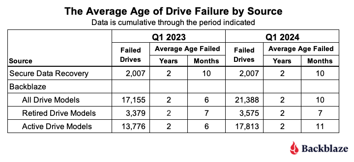
In Q1 2023 Drive Stats report, we took a look at the average age in which a drive fails. This review was inspired by the folks at Secure Data Recovery who calculated that based on their analysis of 2,007 failed drives, the average age at which they failed was 1,051 days or roughly 2 years and 10 months. 

We applied the same approach to our 17,155 failed drives and were surprised when our average age of failure was only 2 years and 6 months. Then we realized that many of the drive models that were still in use were older (much older) than the average, and surely when some number of them failed, it would affect the average age of failure for a given drive model. 

To account for this realization, we considered only those drive models that are no longer active in our production environment. We call this collection retired drive models as these are drives that can no longer age or fail. When we reviewed the average age of this retired group of drives, the average age of failure was 2 years and 7 months. Unexpected, yes, but we decided we needed more data before reaching any conclusions.

So, here we are a year later to see if the average age of drive failure we computed in Q1 2023 has changed. Let’s dig in. 

As before we recorded the date, serial_number, model, drive_capacity, failure, and SMART 9 raw value for all of the failed drives we have in the Drive Stats dataset back to April 2013. The SMART 9 raw value gives us the number of hours the drive was in operation. Then we removed boot drives and drives with incomplete data, that is some of the values were missing or wildly inaccurate. This left us with 17,155 failed drives as of Q1 2023.

Over this past year, Q2 2023 through Q1 2024, we recorded an additional 4,406 failed drives. There were 173 drives which were either boot drives or had incomplete data, leaving us with 4,233 drives to add to the 17,155 failed drives previous, totalling 21,388 failed drives to evaluate.

When we compare Q1 2023 to Q1 2024 we get the table below.

The average age of failure for all of the Backblaze drive models (2 years and 10 months) matches the Secure Data Recovery baseline. The question is, does that validate their number? We say, not yet. Why? Two primary reasons. 

First, we only have two data points, so we don’t have much of a trend, that is we don’t know if the alignment is real or just temporary. Second, the average age of failure of the active drive models (that is, those in production) is now already higher (2 years and 11 months) than the Secure Data baseline. If that trend were to continue, then when the active drive models retire, they will likely increase the average age of failure of the drive models that are not in production.

That said, we can compare the numbers by drive size and drive model from Q1 2023 to Q1 2024 to see if we can gain any additional insights. Let’s start with the average age by drive size in the table below.

The most salient observation is that for every drive size that had active drive models (green), the average age of failure increased from Q1 2023 to Q1 2024. Given that the overall average age of failure increased over the last year, it is reasonable to expect that some of the active drive size cohorts would increase. With that in mind, let’s take a look at the changes by drive model over the same period. 

Starting with the retired drive models, there were three drive models totalling 196 drives which moved from active to retired from Q1 2023 to Q1 2024. Still, the average age of failure for the retired drive cohort remained at 2 years 7 months, so we’ll spare you from looking at a chart with 39 drive models where over 90% of the data didn’t change Q1 2023 to Q1 2024.

On the other hand, the active drive models are a little more interesting, as we can see below.

In all but the two drive models (highlighted), the average age of failure for each drive model went up. In other words, active drive models are, on average, older when they fail, than one year ago. Remember, we are testing the average age of the drive failures, not the average age of the drive. 

At this point, let’s review. The Secure Data Recovery folks checked 2,007 failed drives and determined their average age of failure was 2 years and 10 months. We are testing that assertion. At the moment, the average age of failure for the retired drive models (those no longer in operation in our environment) is 2 years and 7 months. This is still less than the Secure Data number. But, the drive models still in operation are now hitting an average of 2 years and 10 months, suggesting that once these drive models are removed from service, the average age of failure for the retired drive models will increase. 

Based on all of this, we think the average age of failure for our retired drive models will eventually exceed 2 years and 10 months. Further, we predict that the average age of failure will reach closer to 4 years for the retired drive models once our 4TB drive models are removed from service. 

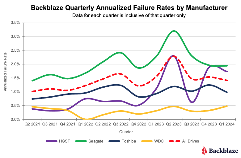
Annualized Failures Rates for Manufacturers

As we noted at the beginning of this report, the quarterly AFR for Q1 2024 was 1.41%. Each of the four manufacturers we track contributed to the overall AFR as shown in the chart below.

As you can see, the overall AFR for all drives peaked in Q3 2023 and is dropping. This is mostly due to the retirement of older 4TB drives that are further along the bathtub curve of drive failure. Interestingly, all of the remaining 4TB drives in use today are either Seagate or HGST models. Therefore, we expect the quarterly AFR will most likely continue to decrease for those two manufacturers as over the next year their 4TB drive models will be replaced.

Lifetime Hard Drive Failure Rates

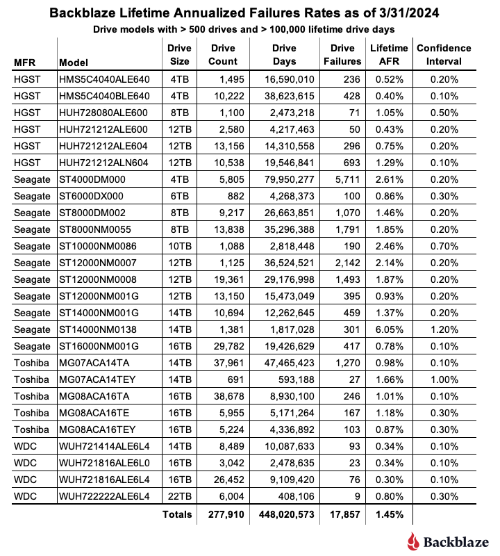
As of the end of Q1 2024, we were tracking 279,572 operational hard drives. As noted earlier, we defined the minimum eligibility criteria of a drive model to be included in our analysis for quarterly, annual and lifetime reviews. To be considered for the lifetime review, a drive model was required to have 500 or more drives as of the end of Q1 2024 and have over 100,000 accumulated drive days during their lifetime. When we removed those drive models which did not meet the lifetime criteria, we had 277,910 drives grouped into 26 models remaining for analysis as shown in the tale below.

With three exceptions, the conference interval for each drive model is 0.5% or less at 95% certainty. For the three exceptions: the 10TB Seagate, the 14TB Seagate, and 14TB Toshiba models, the occurrence of drive failure from quarter to quarter was too variable over their lifetime. This volatility has a negative effect on the confidence interval.

The combination of a low lifetime AFR and a small confidence interval is helpful in identifying the drive models which work well in our environment. These days we are interested mostly in the larger drives as replacements, migration targets, or new installations. Using the table above, let’s see if we can identify our best 12, 14, and 16TB performers. We’ll skip reviewing the 22TB drives as we only have one model.

The drive models are grouped by drive size, then sorted by their Lifetime AFR. Let’s take a look at each of those groups.

  • 12TB drive models: The three 12TB HGST models are great performers, but are hard to find new. Also, Western Digital, who purchased the HGST drive business a while back, has started using their own model numbers of these drives, so it can be confusing. If you do find an original HGST make sure it is new as from our perspective buying a refurbished drive is not the same as buying a new.
  • 14TB drive models: The first three models look to be solid—the WDC (WUH721414ALE6L4), Toshiba (MG07ACA14TA), and Seagate (ST14000NM001G). The remaining two drive models have mediocre lifetime AFRs and undesirable confidence intervals. 
  • 16TB drive models: Lots of choice here, with all six drive models performing well to this point, although the WDC models are the best of the best to date.

The Hard Drive Stats Data

It has now been eleven years since we began recording, storing and reporting the operational statistics of the hard drives and SSDs we use to store data in the Backblaze data storage cloud. We look at the telemetry data of the drives, including their SMART stats and other health related attributes. We do not read or otherwise examine the actual customer data stored. 

Over the years, we have analyzed the data we have gathered and published our findings and insights from our analyses. For transparency, we also publish the data itself, known as the Drive Stats dataset. This dataset is open source and can be downloaded from our Drive Stats webpage.

You can download and use the Drive Stats dataset for free for your own purpose. All we ask are three things: 1) you cite Backblaze as the source if you use the data, 2) you accept that you are solely responsible for how you use the data, and 3) you do not sell this data to anyone; it is free.

Good luck and let us know if you find anything interesting.

The post Backblaze Drive Stats for Q1 2024 appeared first on Backblaze Blog | Cloud Storage & Cloud Backup

The UK Bans Default Passwords

Post Syndicated from Bruce Schneier original https://www.schneier.com/blog/archives/2024/05/the-uk-bans-default-passwords.html

The UK is the first country to ban default passwords on IoT devices.

On Monday, the United Kingdom became the first country in the world to ban default guessable usernames and passwords from these IoT devices. Unique passwords installed by default are still permitted.

The Product Security and Telecommunications Infrastructure Act 2022 (PSTI) introduces new minimum-security standards for manufacturers, and demands that these companies are open with consumers about how long their products will receive security updates for.

The UK may be the first country, but as far as I know, California is the first jurisdiction. It banned default passwords in 2018, the law taking effect in 2020.

This sort of thing benefits all of us everywhere. IoT manufacturers aren’t making two devices, one for California and one for the rest of the US. And they’re not going to make one for the UK and another for the rest of Europe, either. They’ll remove the default passwords and sell those devices everywhere.

Another news article.

Making Life Easier for MSPs: The Zabbix Advantage

Post Syndicated from Michael Kammer original https://blog.zabbix.com/making-life-easier-for-msps-the-zabbix-advantage/28004/

Times have never been better for managed service providers (MSPs). The demand for remote monitoring services has skyrocketed as cloud adoption rises and working from home becomes the new standard. The number of organizations that trust MSPs with the everyday functioning of their mission-critical IT systems and processes has grown rapidly – nearly 9 out of 10 small and medium enterprises either use or plan to use MSPs to manage their infrastructure.

As a service provider, an MSP needs to be ahead of the curve at all times and adopt a constantly-shifting and evolving set of best practices for remote monitoring and management. At Zabbix, we’ve created the ultimate solution for full-stack IT monitoring, and we’ve built in features and benefits that are designed to make it as easy as possible for MSPs to provide top-quality monitoring to their clients as well. Keep reading to learn more about what makes Zabbix the ideal monitoring tool for any MSP.

There are no limits to what you can monitor with Zabbix

And when we say no limits, we mean no limits! Zabbix literally allows you to monitor anything from the frequency of a baby’s cries to the hydraulic systems on a space station. From hardware to software to middleware, VEP resources, virtual resources, and more, Zabbix is capable of monitoring millions of metrics.  As an MSP, you’re no doubt called upon to tackle anything from basic network and server monitoring to highly advanced cloud, container, and Kubernetes monitoring. Zabbix lets you keep it all under one roof and handle it with a single solution.

You can integrate Zabbix with any client’s systems

Today’s MSP needs to be able to seamlessly integrate their tools and processes with the IT frameworks and ITIL guidelines of their clients as well as their business goals, strategies, and best practices. Zabbix is designed to work with third party solutions and boasts a constantly-growing list of official integrations.

When you’re notified of a potential problem, you can easily forward your alerts to third-party ITSM, helpdesk, and messaging systems, enhance them with the additional information that Zabbix is able to collect, and freely customize the outgoing messages for different clients – just one of the areas where Zabbix stands out as an ideal multitenant solution.

Zabbix makes reporting and analysis simple

MSPs need to be able to quickly generate and share regular reports and analyses with clients, keeping them up to speed on the status, performance, and health of their infrastructure. Ideally, those reports should be clear, concise, and actionable, highlighting key metrics and insights via graphs, charts, and tables, identifying trends, and predicting potential issues. Done right, reporting can enhance service quality and position you as an ideal strategic partner.

When you make the decision to deploy Zabbix scheduled reports, you’ll get daily, weekly, monthly, and yearly overviews of the infrastructures and business services you’ve been tasked to monitor. You can also track the changes performed in your Zabbix instance with our robust and detailed built-in audit logging functionality, all of which is designed to make it as easy as possible for you to keep your clients in the loop.

Zabbix makes data easy to visualize

Much like the world around them, MSPs have become increasingly more data-driven. It’s easy to understand why – when you have critical information right in front of you, it’s easier to see trends you would have otherwise missed, which in turn helps you make better-informed decisions that can help guide you to success.

Zabbix dashboards are built to serve as visual storybooks for your business. They transform complex monitoring metrics into an engaging narrative, presenting intimidating data in an intuitive, insightful layout and making data interpretation simple.

You can customize dashboards, screens, and slideshows to easily track the status of a tenant’s infrastructure, applications, and business services. You can also leverage a wide range of dashboard widgets to aggregate, transform, and graph your data while also tracking your monitoring endpoints on geographical and network maps, identifying the status of the most critical alarms, and sorting your monitoring endpoints by resource usage.

Zabbix makes effective security management easier

When it comes to cyberattacks, MSPs are up against a constantly changing threat landscape, not to mention the challenges they face in protecting diverse, multitenant setups. With Zabbix, you can secure connections to and from your monitoring endpoints either with certificates or via pre-shared key encryption.

Multitenant MSPs can also control access to different Zabbix elements and features by creating unique Zabbix roles for your tenants while taking advantage of the native permission logic to isolate monitoring endpoints between tenants. Host groups and subgroups let you decide what your tenants can see, and encrypted agents help to secure all communication, including proxy-to-server communication.

You can also rely on encrypted communication between Zabbix components as well as flexible permissions, user authentication, and integrations with secret vaults for storing passwords and other sensitive information.

Zabbix is inherently scalable

There are no two ways about it – surviving as an MSP in today’s business environment means being able to scale. The number of customers that you support is likely to vary from year to year or even month to month. In order to add customers without compromising your level of service, you need to scale up. And if your customer base shrinks, you will probably need to decrease the size of your infrastructure and operations in order to avoid spending money on services that your business no longer needs.

By deploying Zabbix proxies and letting them collect and process data on behalf of the primary Zabbix server node, you can easily scale your Zabbix instance as your client base expands – no matter where those clients happen to be. And if you need to scale back your business for any reason, it’s a simple matter of deleting the unused proxies.

Zabbix is uniquely cost-efficient

A key benefit of Zabbix has always been that it’s open-source – there are no license fees associated with using our software, and you’re not locked into an endless, inflexible contract. Meanwhile, our extensive range of competitively-priced professional services are designed to fit the unique needs of MSPs and give you the most effective solutions as quickly as possible.

Perhaps most importantly for a multitenant MSP, Zabbix is built to run without the need for a lot of infrastructure or resources. With Zabbix, you can offer your clients more flexibility than comparable monitoring solutions while dramatically lowering the amount of hardware, CPU power, and costs involved.

Conclusion

In order to serve the constantly evolving needs of their clients, MSPs demand more flexibility and features than ever before – and this naturally extends to the monitoring solutions they choose. Rather than offer a few additional services to target MSPs, we’ve built our business with them in mind, which is why we offer a range of feature-rich technical support plans specifically for MSPs.

To learn more about what Zabbix can do for MSPs like yours, visit our website or request a demo.

The post Making Life Easier for MSPs: The Zabbix Advantage appeared first on Zabbix Blog.

„Малките промени“, които отвоюват територия завладяната държава

Post Syndicated from Bozho original https://blog.bozho.net/blog/4290

Чувам скептиците да казват „нищо позитивно не се случи в тези девет месеца за борбата с корупцията“. И макар това обективно да не е вярно твърдение, много промени не стигат до прайм-тайма, защото изглеждат малки.

Премахването на едно изречение за всевластието на главния прокурор и превръщането на колегиите в отделни съвети с „лека“ промяна в квотите (в Конституцията) не звучи грандиозно за неекспертите. Механизма за разследване на главния прокурор – също. Обжалваемостта на отказите на прокуратурата да разследва – също. Повишената прозрачност в Закона за оествените поръчки (вероятно заради която в момента се разследва една варненска болница за незаконни инхауси) – също.

И още: подобряването на закона за защита на подателите на сигнали (вкл. за корупция); разследващите функции на новата антикорупционна комисия; задължението за нова, прозрачна и централизирана система за случайно разпределение на дела; проекта за нов Закон за съдебната власт; електронизацията в много сектори, което ги прави по-проследими и отчетни.

А и добрите промени много лесно се омаловажават. Разследването на главния прокурор е в ход, но тъй като няма повдигнато обвинение, е лесно да се каже, че „не работи“. За промените в Конституцията някой черноглед анализатор казва „ами ето, има проблеми със служебното правителство, значи цалата реформа е таква“. Отказът на ГЕРБ да попълним антикорупционната комисия се представя като дефицит на закона.

Обаче именно малките промени в член едикойси на Конституцията, Наказателно-процесуалния кодекс, Закона за съдебната власт, Закона за обществените поръчки, Закона за противодействие на корупцията и др. са тези, които носят съществената промяна. Заедно с други, косвено-антикорупционни мерки като включването на общинските проекти в Закона за бюджета, законовите промени за премахването на руската корупционна зависимост на енергетиката ни, дигитализацията и др.

Обнародването в Държавен вестник не вкарва никого в затвора и не спира корупцията на другия ден. Но създава необходимите условия за това.

И тук е асиметрията – трябва избирателите да вярват, че правим правилните неща, докато прайм-таймът не само не дава обективна оценка за ефекта от тези промени, а и опитва да ги задраска, защото „не работят“.

Наша работа е да свържем тези победи в разказ за битката срещу завладяната държава, който да не може да бъде отписан с махване на ръка от някой в сутрешен блок. Защото те са именно това – всяка запетая, която е станала закон след дълги преговори, спорове и маневри, е парче територия, което е отнето от паралелната власт.

И вече случилите се промени, и бъдещите – в Закона за съдебната власт и в законите, които в момента позволяват схеми като „Нотариуса“ и „Осемте джуджета“, са част от пътя, по който вървим, с подкрепата, която обществото ни дава.

Материалът „Малките промени“, които отвоюват територия завладяната държава е публикуван за пръв път на БЛОГодаря.

How to Send MMS Using Amazon Pinpoint

Post Syndicated from Tyler Holmes original https://aws.amazon.com/blogs/messaging-and-targeting/how-to-send-mms-using-amazon-pinpoint/

In our digital age, communication has evolved far beyond simple SMS, short for Simple Message Service. The rise of multimedia messaging has transformed the way we share information, express ourselves, and stay connected. MMS, short for Multimedia Messaging Service, is a technology that has become an integral part of our daily lives, enabling us to convey messages that go beyond the confines of plain text. MMS allows senders to transmit a variety of media, including images, videos, audio recordings, and even documents, alongside traditional text. This powerful combination has revolutionized the way we communicate, making it easier to share experiences, ideas, and emotions in a more engaging and visually compelling manner. In a world where visual content is becoming increasingly dominant, MMS has become a crucial tool for companies to communicate with their customers.

What are the differences between SMS and MMS?

MMS is similar to SMS but has some very distinct differences that enable you to send and engage with your customers in different ways.

Message length

  • SMS
    • SMS can send text messages up to 160 characters as long as each character is a part of the GSM 03.38 character set. This means that if you have long links or longer form content that you need to send that these messages will be broken up into multiple message parts. This increases your cost and decreases the recipient reading experience on their device.
  • If your SMS contains any characters that are outside of the GSM 03.38 character set, your message can only contain up to 70 characters. Depending on the language you are using this can be very limiting. Messages that are broken up into multiple message parts can quickly cause you to hit your throughput limits since each part is measured as one message, even if you are only making a single call to the API. A GSM 03.38 message with 161 characters is 2 message parts which means that your throughput is effectively cut in half.
  • MMS
    • MMS can send up to 1,600 characters, regardless of the character set you use. Messages can be much larger, often up to 300 KB depending on the character set you are using. This expanded size allows you to send long form messages and not be so limited if you need to send messages in a character set outside of GSM 03.38 or just have the need to send longer messages.
    • This can reduce your cost and improve the experience for your recipients.
    • The larger message size helps you manage your throughput limitations since, a single MMS message can be sent, rather than an SMS being broken up into multiple message parts.

Message content

  • SMS
    • SMS is text based only. You cannot send media or attachments.
  • MMS
    • MMS can send multimedia content such as images, videos, PDF files, and audio files. This opens up many more options for how it can be used such as attaching a receipt, sending a new product launch gallery, or supporting troubleshooting with a how-to video.
    • A single MMS message can be up to 600KB in size for media files
    • Supported media file formats
      • Portable Network Graphics (PNG)
      • Joint Photographic Experts Group (JPEG)
      • Graphics Interchange Format (GIF)
      • MPEG-4 (MP4)
      • Quicktime File Format (MOV)
      • Portable Document Format (PDF)
      • Virtual Contact File (VCF)
      • More

Message delivery time

  • SMS
    • SMS messages are delivered as a text-only message and are much smaller which may result in it being delivered more promptly.
  • MMS
    • MMS messages may take longer to deliver dependent on the type and size of the multimedia content that is included which may increase the time to be delivered. This makes time sensitive messages such as OTP delivery more costly and potentially slower so it’s not an ideal use case for MMS.

Cost

Network and device support

  • SMS
    • SMS is a widely-adopted and supported protocol across all mobile networks
    • SMS is compatible with all mobile devices, even the most basic models
  • MMS
    • MMS requires specific network infrastructure and compatibility between the sender’s and receiver’s devices and networks
    • MMS requires devices with multimedia capabilities, such as smartphones or feature phones with advanced messaging capabilities. Long text MMS messages sent to an MMS incapable recipient will be redirected to SMS by default

Regional availability and location

What are some examples of MMS messages?

Here are some examples of how MMS messages can be used:

  • Attached video
    • “Introducing our new limited-edition product line! 📽 Check out this exclusive sneak peek video.“
  • Single attached photo
    • “Caught you in the act! 👀 Here’s a fun photo from our recent in-store event. Thanks for stopping by!”
  • Multiple attached photos
    • “Treat yourself to something special this weekend. 💄 Explore our latest makeup collection with this handy lookbook.”
  • Attached receipt
    • “Thanks for your most recent purchase! We hope you love it! Your receipt is attached”

It’s important to note that you do not need to send all of your messages using one or the other. As an example you can use SMS for One Time Password (OTP) sends since they do not require media and generally should be a single message part in any language and use MMS to enable an eye catching marketing release with pictures or video.

How to send MMS with Amazon Pinpoint

You can use the AWS CLI or Amazon Pinpoint SMS and voice v2 API to send MMS messages to your customers. Use the send-media-message AWS CLI command to send an MMS message. There are two ways to send MMS depending on whether you are including media with your message.

How to send MMS with media

The first step to sending MMS is to make sure that you have an Origination Identity (OID) that is enabled for MMS. Amazon Pinpoint supports sending MMS to the US and Canada. Eligible MMS numbers in the US include 10DLC, toll-free, and short codes. Canadian eligible MMS numbers include long codes and short codes.

NOTE: If you procured originators for the US and Canada prior to May 2024, in some cases, existing Pinpoint SMS US and Canadian phone will be automatically updated to begin supporting MMS. To determine if your existing Amazon Pinpoint number(s) are eligible, navigate to the Amazon Pinpoint console Phone Numbers page. If MMS is listed under the “capabilities” column, you can begin using that number for MMS immediately if your number is in an active state. For these existing eligible numbers, there is no additional registration requirement as long as your use case doesn’t change. If the capability listed only shows SMS, you will need to procure a new US or Canadian phone number which will automatically include MMS.

For all newly purchased(Post May 2024) Amazon Pinpoint US and Canadian phone numbers, both SMS and MMS services will automatically be added at time of purchase, simplifying the registration process and providing the flexibility to use either messaging formats upon approval.

You can get started by navigating to the Pinpoint SMS console phone number page and selecting Request Originator. From there, simply follow the self-guided steps for purchasing and registering the phone number If you need help determining what type of OID you need consult this tutorial. Information on registering for MMS enabled OIDs can be found here:

Sending MMS with media included requires you to create a bucket in Simple Storage Service (S3) that your media can be accessed from. The media files have to be stored in a publicly available S3 bucket. Information on creating a bucket and uploading media objects to it can be found here:

You will include the link to this bucket in your “sendMediaMessage” call using the “MediaUrls” attribute seen below. The supported media files formats can be found here.

The only required attributes are:

The CLI command below will send an MMS with the text of “Check out this Photo!” and will have a JPEG image included.

aws pinpoint-sms-voice-v2 —region 'xx-xxxx-xx' send-media-message —destination-phone-number +xxxxxxxxxxx —origination-identity +xxxxxxxxxxx —message-body 'Check out this Photo!' —media-urls 's3://s3-bucket/media_file.jpg'

If Amazon Pinpoint SMS accepts the command you will receive the MessageID. This only means the command was successfully received and not that the destination device has received the message yet.

How to send an MMS with no media

Sending an MMS with no media attached is nearly the same, you just don’t include a link to an S3 bucket in the “MediaUrls” attribute, it’s as easy as that. You might do this to reduce costs if you are sending a message with characters that are outside of the GSM 03.38 character or on a long message with more than 160 GSM 03.38 characters like the below.

The CLI command below will send the following message:

“This message will be broken up into more than 3 message parts if sent via SMS so we are going to use MMS instead to save costs. This is a great way to reduce your costs even if you are not sending any media such as a photo or video attached. Though a single MMS message costs more than a single SMS message there are times where you may want to use MMS simply because it is a cheaper way of communicating with your recipients. Since you can use SMS and MMS for different scenarios you may choose to send an OTP message with SMS and something like this message using MMS.”

aws pinpoint-sms-voice-v2 —region 'xx-xxxx-xx' send-media-message —destination-phone-number +xxxxxxxxxxx —origination-identity +xxxxxxxxxxx —message-body 'This message will be broken up into more than 3 message parts if sent via SMS so we are going to use MMS instead to save costs. This is a great way to reduce your costs even if you are not sending any media such as a photo or video attached. Though a single MMS message costs more than a single SMS message there are times where you may want to use MMS simply because it is a cheaper way of communicating with your recipients. Since you can use SMS and MMS for different scenarios you may choose to send an OTP message with SMS and something like this message using MMS.'

Conclusion

In this post you learned about the differences between SMS and MMS and how each can be used to send different types of messages. MMS is an excellent channel to communicate with your recipients to send highly engaging content that in some scenarios can reduce your cost while improving your customers’ experience. If you are sending content outside of the GSM 03.38 character set, want to send images, videos, or attachments such as receipts then MMS is definitely something you should look into.

A few resources to help you plan for your SMS program:

Leaky HPE SGI Cheyenne Supercomputer for Sale at Perhaps a Deal

Post Syndicated from Cliff Robinson original https://www.servethehome.com/leaky-hpe-sgi-cheyenne-supercomputer-for-sale-at-perhaps-a-deal-intel-supermicro-mellanox/

A leaky HPE SGI Cheyenne Supercomputer is on auction for about the price of a single NVIDIA H100 GPU system

The post Leaky HPE SGI Cheyenne Supercomputer for Sale at Perhaps a Deal appeared first on ServeTheHome.

Automate Terraform Deployments with Amazon CodeCatalyst and Terraform Community action

Post Syndicated from Vineeth Nair original https://aws.amazon.com/blogs/devops/automate-terraform-deployments-with-amazon-codecatalyst-and-terraform-community-action/

Amazon CodeCatalyst integrates continuous integration and deployment (CI/CD) by bringing key development tools together on one platform. With the entire application lifecycle managed in one tool, CodeCatalyst empowers rapid, dependable software delivery. CodeCatalyst offers a range of actions which is the main building block of a workflow, and defines a logical unit of work to perform during a workflow run. Typically, a workflow includes multiple actions that run sequentially or in parallel depending on how you’ve configured them.

Introduction

Infrastructure as code (IaC) has become a best practice for managing IT infrastructure. IaC uses code to provision and manage your infrastructure in a consistent, programmatic way. Terraform by HashiCorp is one of most common tools for IaC.

With Terraform, you define the desired end state of your infrastructure resources in declarative configuration files. Terraform determines the necessary steps to reach the desired state and provisions the infrastructure automatically. This removes the need for manual processes while enabling version control, collaboration, and reproducibility across your infrastructure.

In this blog post, we will demonstrate using the “Terraform Community Edition” action in CodeCatalyst to create resources in an AWS account.

Amazon CodeCatalyst workflow overview
Figure 1: Amazon CodeCatalyst Action

Prerequisites

To follow along with the post, you will need the following items:

Walkthrough

In this walkthrough we create an Amazon S3 bucket using the Terraform Community Edition action in Amazon CodeCatalyst. The action will execute the Terraform commands needed to apply your configuration. You configure the action with a specified Terraform version. When the action runs it uses that Terraform version to deploy your Terraform templates, provisioning the defined infrastructure. This action will run terraform init to initialize the working directory, terraform plan to preview changes, and terraform apply to create the Amazon S3 bucket based on the Terraform configuration in a target AWS Account. At the end of the post your workflow will look like the following:

Amazon CodeCatalyst Workflow with Terraform Community Action

Figure 2: Amazon CodeCatalyst Workflow with Terraform Community Action

Create the base workflow

To begin, we create a workflow that will execute our Terraform code. In the CodeCatalyst project, click on CI/CD on left pane and select Workflows. In the Workflows pane, click on Create Workflow.

Creating Amazon CodeCatalyst Workflow

Figure 3: Creating Amazon CodeCatalyst Workflow

We have taken an existing repository my-sample-terraform-repository as a source repository.

Creating Workflow from source repository

Figure 4 : Creating Workflow from source repository

Once the source repository is selected, select Branch as main and click Create. You will have an empty workflow. You can edit the workflow from within the CodeCatalyst console. Click on the Commit button to create an initial commit:

Initial Workflow commit

Figure 5: Initial Workflow commit

On the Commit Workflow dialogue, add a commit message, and click on Commit. Ignore any validation errors at this stage:

Completing Initial Commit for Workflow

Figure 6: Completing Initial Commit for Workflow

Connect to CodeCatalyst Dev Environment

For this post, we will use an AWS Cloud9 Dev Environment to edit our workflow. Your first step is to connect to the dev environment. Select Code → Dev Environments.

Navigate to CodeCatalyst Dev Environments

Figure 7 : Navigate to CodeCatalyst Dev Environments

If you do not already have a Dev Environment you can create an instance by selecting the Create Dev Environment dropdown and selecting AWS Cloud9 (in browser). Leave the options as default and click on Create to provision a new Dev Environment.

Create CodeCatalyst Dev Environment

Figure 8: Create CodeCatalyst Dev Environment

Once the Dev Environment has provisioned, you are redirected to a Cloud9 instance in browser. The Dev Environment automatically clones the existing repository for the Terraform project code. We at first create a main.tf file in root of the repository with the Terraform code for creating an Amazon S3 bucket. To do this, we right click on the repository folder in the tree-pane view on the left side of the Cloud9 Console window and select New File

Creating a new file in Cloud9

Figure 9: Creating a new file in Cloud9

We are presented with a new file which we will name main.tf, this file will store the Terraform code. We then edit main.tf by right clicking on the file and selecting open. We insert the code below into main.tf. The code has a Terraform resource block to create an AWS S3 Bucket. The configuration also uses Terraform AWS datasources to obtain AWS region and AWS Account ID data which is used to form part of the bucket name. Finally, we use a backend block to configure Terraform to use an AWS S3 bucket to store Terraform state data. To save our changes we select File -> Save

: Adding Terraform Code

Figure 10: Adding Terraform Code

Now let’s start creating Terraform Workflow using Amazon CodeCatalyst Terraform Community Action. Within your repository go to .codecatalyst/workflows directory and open the <workflowname.yaml> file.

Creating CodeCatalyst Workflow

Figure 11: Creating CodeCatalyst Workflow

The below code snippet is an example workflow definition with terraform plan and terraform apply. We will enter this into our workflow file, with the relevant configuration settings for our environment.

The workflow does the following:

  • When a change is pushed to the main branch, a new workflow execution is triggered. This workflow carries a Terraform plan and subsequent apply operation.
    Name: terraform-action-workflow
    Compute:
      Type: EC2
      Fleet: Linux.x86-64.Large
    SchemaVersion: "1.0"
    Triggers:
      - Type: Push
        Branches:
          -  main
    Actions: 
      PlanTerraform:
        Identifier: codecatalyst-labs/provision-with-terraform-community@v1
        Environment:
          Name: dev 
          Connections:
            - Name: codecatalyst
              Role: CodeCatalystWorkflowDevelopmentRole # The IAM role to be used
        Inputs:
          Sources:
            - WorkflowSource
        Outputs:
          Artifacts:
            - Name: tfplan # generates a tfplan output artifact
              Files:
                - tfplan.out
        Configuration:
          AWSRegion: eu-west-2
          StateBucket: tfstate-bucket # The Terraform state S3 Bucket
          StateKey: terraform.tfstate # The Terraform state file
          StateKeyPrefix: states/ # The path to the state file (optional)
          StateTable: tfstate-table # The Dynamo DB database
          TerraformVersion: ‘1.5.1’ # The Terraform version to be used
          TerraformOperationMode: plan # The Terraform operation- can be plan or apply
      ApplyTerraform:
        Identifier: codecatalyst-labs/provision-with-terraform-community@v1
        DependsOn:
          - PlanTerraform
        Environment:
          Name: dev 
          Connections:
            - Name: codecatalyst
              Role: CodeCatalystWorkflowDevelopmentRole
        Inputs:
          Sources:
            - WorkflowSource
          Artifacts:
            - tfplan
        Configuration:
          AWSRegion: eu-west-2
          StateBucket: tfstate-bucket
          StateKey: terraform.tfstate
          StateKeyPrefix: states/
          StateTable: tfstate-table
          TerraformVersion: '1.5.1'
          TerraformOperationMode: apply
  • Key configuration parameters are:
    • Environment.Name: The name of our CodeCatalyst Environment
    • Environment.Connections.Name: The name of the CodeCatalyst connection
    • Environment.Connections.Role: The IAM role used for the workflow
    • AWSRegion: The AWS region that hosts the Terraform state bucket
    • Environment.Name: The name of our CodeCatalyst Environment
    • Identifier: codecatalyst-labs/provision-with-terraform-community@v1
    • StateBucket: The Terraform state bucket
    • StateKey: The Terraform statefile e.g. terraform.tfstate
    • StateKeyPrefix: The folder location of the State file (optional)
    • StateTable: The DynamoDB State table
    • TerraformVersion: The version of Terraform to be installed
    • TerraformOperationMode: The operation mode for Terraform – this can be either ‘plan’ or ‘apply’

The workflow now contains CodeCatalyst action for Terraform Plan and Terraform Apply.

To save our changes we select File -> Save, we can then commit these to our git repository by typing the following at the terminal:

git add . && git commit -m ‘adding terraform workflow and main.tf’ && git push

The above command adds the workflow file and Terraform code to be tracked by git. It then commits the code and pushes the changes to CodeCatalyst git repository. As we have a branch trigger for main defined, this will trigger a run of the workflow. We can monitor the status of the workflow in the CodeCatalyst console by selecting CICD -> Workflows. Locate your workflow and click on Runs to view the status. You will be able to observe that the workflow has successfully completed and Amazon S3 bucket is created.

: CodeCatalyst Workflow Status

Figure 12: CodeCatalyst Workflow Status

Cleaning up

If you have been following along with this workflow, you should delete the resources that you have deployed to avoid further charges. The walkthrough will create an Amazon S3 bucket named <your-aws-account-id>-<your-aws-region>-terraform-sample-bucket in your AWS account. In the AWS Console > S3, locate the bucket that was created, then select and click Delete to remove the bucket.

Conclusion

In this post, we explained how you can easily get started deploying IaC to your AWS accounts with Amazon CodeCatalyst. We outlined how the Terraform Community Edition action can streamline the process of planning and applying Terraform configurations and how to create a workflow that can leverage this action. Get started with Amazon CodeCatalyst today.

Richard Merritt

Richard Merritt is a Senior DevOps Consultant at Amazon Web Services (AWS), Professional Services. He works with AWS customers to accelerate their journeys to the cloud by providing scalable, secure and robust DevOps solutions.

Vineeth Nair

Vineeth Nair is a DevOps Architect at Amazon Web Services (AWS), Professional Services. He collaborates closely with AWS customers to support and accelerate their journeys to the cloud and within the cloud ecosystem by building performant, resilient, scalable, secure and cost efficient solutions.

Nagaraju Basavaraju

Nagaraju is a seasoned DevOps Architect at AWS, UKI. He specializes in assisting customers in designing and implementing secure, scalable, and resilient hybrid and cloud-native solutions with DevOps methodologies. With a profound passion for cloud infrastructure, observability and automation, Nagaraju is also an avid contributor to Open-Source projects related to Terraform and AWS CDK.

Debojit Bhadra

Debojit is a DevOps consultant who specializes in helping customers deliver secure and reliable solutions using AWS services. He concentrates on infrastructure development and building serverless solutions with AWS and DevOps. Apart from work, Debojit enjoys watching movies and spending time with his family.

GNU nano 8.0 released

Post Syndicated from jzb original https://lwn.net/Articles/971980/

Version 8.0 of the terminal text editor GNU nano has been
released. This update includes several changes to keybindings to be
more newcomer-friendly, such as remapping Ctrl-F to forward-search and
adding an option for modern bindings:

Command-line option –modernbindings (-/) makes ^Q quit, ^X cut,
^C copy, ^V paste, ^Z undo, ^Y redo, ^O open a file, ^W write a
file, ^R replace, ^G find again, ^D find again backwards, ^A set
the mark, ^T jump to a line, ^P show the position, and ^E execute.

The release also provides access to 14 levels of gray scale in xterm (up
from four), as well as many bug fixes.

Analyze more demanding as well as larger time series workloads with Amazon OpenSearch Serverless 

Post Syndicated from Satish Nandi original https://aws.amazon.com/blogs/big-data/analyze-more-demanding-as-well-as-larger-time-series-workloads-with-amazon-opensearch-serverless/

In today’s data-driven landscape, managing and analyzing vast amounts of data, especially logs, is crucial for organizations to derive insights and make informed decisions. However, handling this data efficiently presents a significant challenge, prompting organizations to seek scalable solutions without the complexity of infrastructure management.

Amazon OpenSearch Serverless lets you run OpenSearch in the AWS Cloud, without worrying about scaling infrastructure. With OpenSearch Serverless, you can ingest, analyze, and visualize your time-series data. Without the need for infrastructure provisioning, OpenSearch Serverless simplifies data management and enables you to derive actionable insights from extensive repositories.

We recently announced a new capacity level of 10TB for Time-series data per account per Region, which includes one or more indexes within a collection. With the support for larger datasets, you can unlock valuable operational insights and make data-driven decisions to troubleshoot application downtime, improve system performance, or identify fraudulent activities.

In this post, we discuss this new capability and how you can analyze larger time series datasets with OpenSearch Serverless.

10TB Time-series data size support in OpenSearch Serverless

The compute capacity for data ingestion and search or query in OpenSearch Serverless is measured in OpenSearch Compute Units (OCUs). These OCUs are shared among various collections, each containing one or more indexes within the account. To accommodate larger datasets, OpenSearch Serverless now supports up to 200 OCUs per account per AWS Region, each for indexing and search respectively, doubling from the previous limit of 100. You configure the maximum OCU limits on search and indexing independently to manage costs. You can also monitor real-time OCU usage with Amazon CloudWatch metrics to gain a better perspective on your workload’s resource consumption.

Dealing with larger data and analysis needs more memory and CPU. With 10TB data size support, OpenSearch Serverless is introducing vertical scaling up to eight times of 1-OCU systems. For example, the OpenSearch Serverless will deploy a larger system equivalent of eight 1-OCU systems. The system will use hybrid of horizontal and vertical scaling to address the needs of the workloads. There are improvements to shard reallocation algorithm to reduce the shard movement during heat remediation, vertical scaling, or routine deployment.

In our internal testing for 10TB Time-series data, we set the Max OCU to 48 for Search and 48 for Indexing. We set the data retention for 5 days using data lifecycle policies, and set the deployment type to “Enable redundancy” making sure the data is replicated across Availability Zones . This will lead to 12_24 hours of data in hot storage (OCU disk memory) and the rest in Amazon Simple Service (Amazon S3) storage. We observed the average ingestion achieved was 2.3 TiB per day with an average ingestion performance of 49.15 GiB per OCU per day, reaching a max of 52.47 GiB per OCU per day and a minimum of 32.69 Gib per OCU per day in our testing. The performance depends on several aspects, like document size, mapping, and other parameters, which may or may not have a variation for your workload.

Set max OCU to 200

You can start using our expanded capacity today by setting your OCU limits for indexing and search to 200. You can still set the limits to less than 200 to maintain a maximum cost during high traffic spikes. You only pay for the resources consumed, not for the max OCU configuration.

Ingest the data

You can use the load generation scripts shared in the following workshop, or you can use your own application or data generator to create a load. You can run multiple instances of these scripts to generate a burst in indexing requests. As shown in the following screenshot, we tested with an index, sending approximately 10 TB of data. We used our load generator script to send the traffic to a single index, retaining data for 5 days, and used a data life cycle policy to delete data older than 5 days.

Auto scaling in OpenSearch Serverless with new vertical scaling.

Before this release, OpenSearch Serverless auto-scaled by horizontally adding the same-size capacity to handle increases in traffic or load. With the new feature of vertical scaling to a larger size capacity, it can optimize the workload by providing a more powerful compute unit. The system will intelligently decide whether horizontal scaling or vertical scaling is more price-performance optimal. Vertical scaling also improves auto-scaling responsiveness, because vertical scaling helps to reach the optimal capacity faster compared to the incremental steps taken through horizontal scaling. Overall, vertical scaling has significantly improved the response time for auto_scaling.

Conclusion

We encourage you to take advantage of the 10TB index support and put it to the test! Migrate your data, explore the improved throughput, and take advantage of the enhanced scaling capabilities. Our goal is to deliver a seamless and efficient experience that aligns with your requirements.

To get started, refer to Log analytics the easy way with Amazon OpenSearch Serverless. To get hands-on experience with OpenSearch Serverless, follow the Getting started with Amazon OpenSearch Serverless workshop, which has a step-by-step guide for configuring and setting up an OpenSearch Serverless collection.

If you have feedback about this post, share it in the comments section. If you have questions about this post, start a new thread on the Amazon OpenSearch Service forum or contact AWS Support.


About the authors

Satish Nandi is a Senior Product Manager with Amazon OpenSearch Service. He is focused on OpenSearch Serverless and has years of experience in networking, security and ML/AI. He holds a Bachelor’s degree in Computer Science and an MBA in Entrepreneurship. In his free time, he likes to fly airplanes, hang gliders and ride his motorcycle.

Michelle Xue is Sr. Software Development Manager working on Amazon OpenSearch Serverless. She works closely with customers to help them onboard OpenSearch Serverless and incorporates customer’s feedback into their Serverless roadmap. Outside of work, she enjoys hiking and playing tennis.

Prashant Agrawal is a Sr. Search Specialist Solutions Architect with Amazon OpenSearch Service. He works closely with customers to help them migrate their workloads to the cloud and helps existing customers fine-tune their clusters to achieve better performance and save on cost. Before joining AWS, he helped various customers use OpenSearch and Elasticsearch for their search and log analytics use cases. When not working, you can find him traveling and exploring new places. In short, he likes doing Eat → Travel → Repeat.