When an administrator introduces a rule change in AWS Network Firewall and network connectivity is disrupted, pinpointing the cause requires inspecting multiple points in the traffic path. The firewall gives you stateless and stateful rule engines, domain rules, and routing to the firewall endpoint inside your Amazon Virtual Private Cloud (Amazon VPC). A network drop looks the same from the workload no matter where it started. Isolating the cause means correlating the alert and flow logs with the firewall configuration, route tables, and recent API calls in AWS CloudTrail that might have changed them. That manual correlation is exactly where AWS DevOps Agent helps, accelerating root cause analysis so you can restore connectivity in minutes instead of hours.
AWS DevOps Agent does that correlation for you. As your always-available operations teammate, it resolves and proactively prevents operational issues across AWS, multicloud, and on-premises environments. When an Amazon CloudWatch alarm triggers, it reaches the agent through a webhook. The agent then reads the firewall configuration and logs through AWS APIs, ties the drop to recent API activity, and returns a root cause with a mitigation plan you review before you apply it.
This post connects CloudWatch monitoring to DevOps Agent. It walks through three Network Firewall failures from end to end. The first is a domain deny list blocking a legitimate endpoint. The second is a stateless rule priority misconfiguration. The third is an asymmetric cross Availability Zone (AZ) routing drop. Each maps to a different layer, so each leads down a different investigation path. An AWS Cloud Development Kit (AWS CDK) app deploys the whole environment in your own account so you can reproduce each failure and follow along.
The sample workload
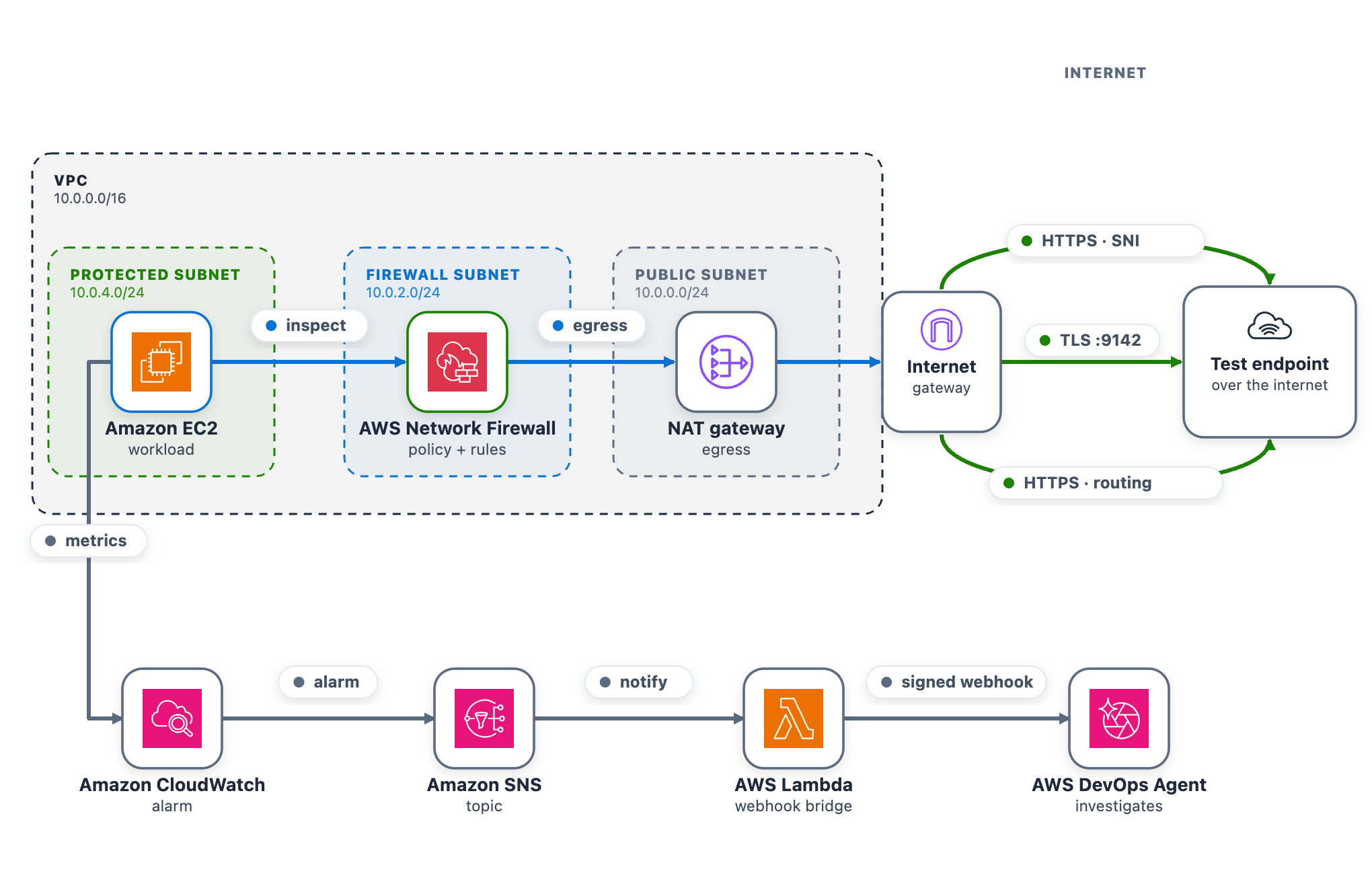
As part of this blog post, we provide a CDK stack that deploys both the AWS DevOps Agent Space and a sample workload used to walk through three separate troubleshooting scenarios. A single t3.micro instance in a protected subnet checks its connectivity to a test endpoint on a continuous loop and publishes results to CloudWatch. Traffic takes the internet egress path through Network Firewall, the NAT gateway, and the internet gateway, so the firewall can intercept or drop it. After completing the walkthrough, you can apply the same troubleshooting techniques with DevOps Agent against your own Network Firewall deployments.
The test endpoint runs in a separate VPC deployed by the same CDK app. It serves HTTPS on port 443 and TCP on port 9142, giving each scenario a different protocol layer to exercise: Scenario 1 targets a TLS connection on 443 (matched by Server Name Indication), Scenario 2 targets a TCP connection on 9142, and Scenario 3 exercises the whole egress path.
A live status page shows one card per scenario plus the network topology. The whole stack deploys from a single CDK app across two Availability Zones, each with a firewall endpoint and NAT gateway, which is what makes Scenario 3 possible.
As shown in the following figure, the egress data path runs from the workload through Network Firewall and the NAT and internet gateways to the test endpoint. The alarm pipeline runs from CloudWatch through Amazon Simple Notification Service (Amazon SNS) and the webhook AWS Lambda function to DevOps Agent.
Figure 1: The sample workload
To use this with your own workload, you need a CloudWatch alarm that detects the connectivity problem and the webhook pipeline (SNS topic and Lambda function) that delivers it to DevOps Agent. The agent reads your firewall configuration, logs, and CloudTrail through AWS APIs, so no additional instrumentation is needed on the firewall side.
AWS CDK 2.x is required. You can use it through the project’s npx dependency, or install it globally:
npm install -g aws-cdk
Deploy the sample workload
Clone the project and deploy it into us-east-1 with one command (set awsRegion to use another AWS Region).
git clone https://github.com/aws-samples/sample-accelerating-aws-network-firewall-troubleshooting-with-aws-devops-agent.git
cd sample-accelerating-aws-network-firewall-troubleshooting-with-aws-devops-agent
bash scripts/deploy.sh
The script checks prerequisites, installs dependencies, compiles and tests, and bootstraps the CDK if needed. It then deploys all the stacks from a clean baseline and prints the outputs, including the status-page URL and sign-in details.
Open the status-page link (an https://<random-id>.cloudfront.net address).
Sign in using the username and password provided from the CDK output and confirm all three cards show the green Healthy status.
Keep the page open while you run the scenarios.
Connect AWS DevOps Agent
To connect AWS DevOps Agent to the alarm pipeline
In the AWS DevOps Agent console, open the nf-devops-agent-space Agent Space created by the CDK deployment.
On the status page, choose Configure webhook, paste the URL and signing secret, and save. The page writes them to the nf-devops-agent-webhook-credentialsAWS Secrets Manager secret, so there is no AWS CLI or console step. Until you set it, the bridge Lambda function sees a placeholder and skips delivery.
Verify the path before you run a scenario. In the Lambda console, open nf-devops-agent-webhook and use the Test tab with this event.
{
  "Records": [
    {
      "Sns": {
        "Message": "{\"AlarmName\":\"TEST-webhook-verification\",\"AlarmDescription\":\"[TEST] Webhook integration test - not a real alarm.\",\"NewStateValue\":\"ALARM\",\"NewStateReason\":\"[TEST] Manual webhook connectivity test. Safe to ignore.\",\"Region\":\"us-east-1\"}"
      }
    }
  ]
}
A 200 response confirms the path, and a test investigation appears in the DevOps Agent Operator Web App view.
How the alarm pipeline works
Every scenario reaches DevOps Agent the same way. A CloudWatch alarm moves to ALARM and notifies the SNS topic. Amazon SNS invokes a Lambda function. The function reads the webhook URL and signing secret from Secrets Manager, signs an alarm payload, and POSTs it to the DevOps Agent webhook (as shown in Figure 1). Amazon SNS also provides delivery retries, fan-out to other subscribers, and cross-account publishing.
Prebuilt Network Firewall metric (Scenario 1) – Alarm-1 watches the DroppedPackets metric, summed across the stateful streams, and triggers when drops rise above a baseline threshold. This requires no workload or custom metric and works on an already-deployed firewall. However, it only tells you that the firewall is dropping packets, not which rule is responsible.
Application health metric (Scenarios 2 and 3) – Alarm-2 and Alarm-3 watch a custom metric from a connectivity check. Use this for an alarm tied to user-facing impact or to tell one traffic path from another, which requires running a component that emits the metric.
Alarm
Source
Triggers when
Alarm-1
Native AWS/NetworkFirewall DroppedPackets
The firewall’s dropped-packet count rises above the baseline
Alarm-2
Custom application health metric
The port 9142 (TCP) connectivity check to the test endpoint is being dropped
Alarm-3
Custom application health metric
The cross Availability Zone connectivity check is being dropped
Run the scenarios
Work through each of the scenarios one at a time, following the same cycle. Interrupt network connectivity, watch the alarm trigger, let DevOps Agent investigate, apply the recommended fix, and confirm recovery before moving on.
The status-page cards follow the live CloudWatch alarm state. A card shows a green dot and the word Healthy when its alarm is clear, and a red dot and the word DROPPED when its alarm triggers. In the DROPPED state the card also adds a Condition: line describing what’s being dropped, which isn’t shown when the card is healthy. Network Firewall applies changes to new flows, so a change shows within a minute or two. Recovery comes from the mitigation DevOps Agent recommends, which you review and apply.
Scenario 1. Domain deny list blocking a legitimate endpoint
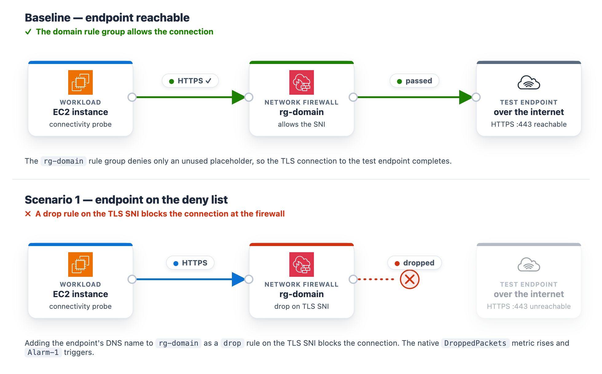
At baseline, the rg-domain Suricata domain rule group denies only an unused placeholder, so the test endpoint stays reachable. The rule group inspects the TLS Server Name Indication (SNI) on each outbound connection and drops any that matches a denied domain. The exact rule syntax and console steps follow.
In the navigation pane, under Network Firewall, choose Network Firewall rule groups.
Choose the rg-domain rule group to open its details page.
In the Rules section, choose Edit.
The rules box already contains two baseline placeholder rules (they match blocked.placeholder.invalid, so nothing real is denied). Leave those in place. Find the <app-endpoint-dns> value for Scenario 1 in the deployment script output (a Nework Load Balancer (NLB) DNS name such as NfTest-AppNl-a1b2C3dEf4G5-1234abcd5678efgh.elb.us-east-1.amazonaws.com). On a new line below the existing rules, add a drop rule that matches that DNS name on the TLS SNI, then choose Save.
drop tls $HOME_NET any -> $EXTERNAL_NET any (ssl_state:client_hello; tls.sni; content:"<app-endpoint-dns>"; startswith; nocase; endswith; msg:"S1 domain denylist"; flow:to_server, established; sid:2000002; rev:1;)
After saving, the rules box holds all three lines. The two placeholders remain, plus the new drop rule for the endpoint DNS name (note the distinct sid 2000002).
What happens. The workload’s HTTPS check to the test endpoint times out, the “AWS/NetworkFirewall DroppedPackets metric climbs above baseline, and Alarm-1 moves to ALARM. The Scenario 1 card reads DROPPED (with the condition Firewall dropping the monitored domain on its allow/deny rules), while the Scenario 2 and Scenario 3 cards stay Healthy (Figure 3). On the topology, the alarm pipeline from CloudWatch through Amazon SNS and Lambda to DevOps Agent and the workload-to-firewall inspect lines both turn amber, which the legend defines as collateral / alarm active, because the packets are now dropped at the firewall. To demonstrate the resulting failure, the HTTPS · SNI line from the internet gateway to the test endpoint is shown in red, which the legend defines as dropped (root cause).
Figure 3: Scenario 1 active – Traffic blocked at the firewall
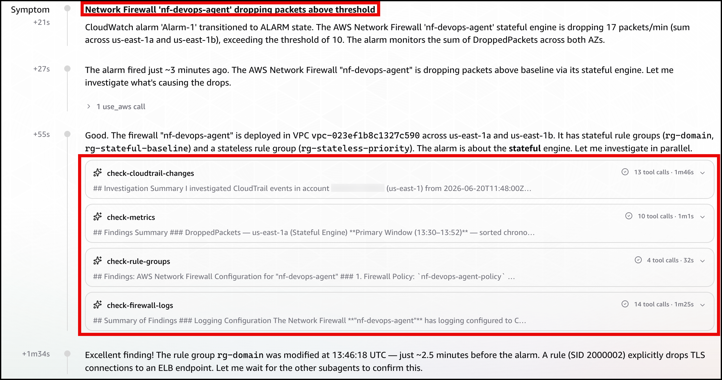
Let DevOps Agent investigate. The agent runs several lines of investigation in parallel and correlates them:
Reads the DroppedPackets metric and correlates the spike with a simultaneous drop in passed packets, confirming the firewall is actively blocking traffic.
Reads the ALERT log and finds the workload’s TLS connections to the test endpoint blocked by the S1 domain denylist rule.
Compares the current state against a baseline window, where the same endpoint was reachable with no alerts, which shows the block is new.
Searches CloudTrail and surfaces the UpdateRuleGroup call that added the deny rule, identifying the user, role, and timestamp approximately one minute before the drops began.
Reports the root cause as that manual rule-group change. Recommends removing the deny entry or adding an allow exception and enabling FirewallPolicyChangeProtection to prevent unauthorized changes.
Presents this as a plan you review and apply, not an automatic change.
In the DevOps Agent Operator Web App view, the agent first restates the Alarm-1 trigger and confirms the firewall is dropping packets above the threshold (Figure 4).
Figure 4: Scenario 1 – The symptom
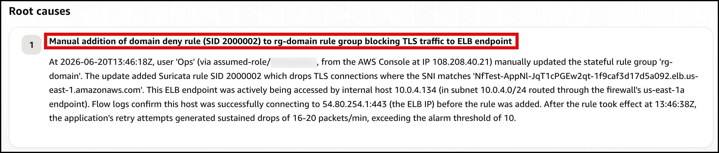
Next, the agent identifies the root cause: a manual update to the rg-domain rule group that added a domain deny rule (SID 2000002) shortly before the alarm fired, blocking TLS connections to the ELB endpoint (Figure 5).
Figure 5: Scenario 1 – The root cause
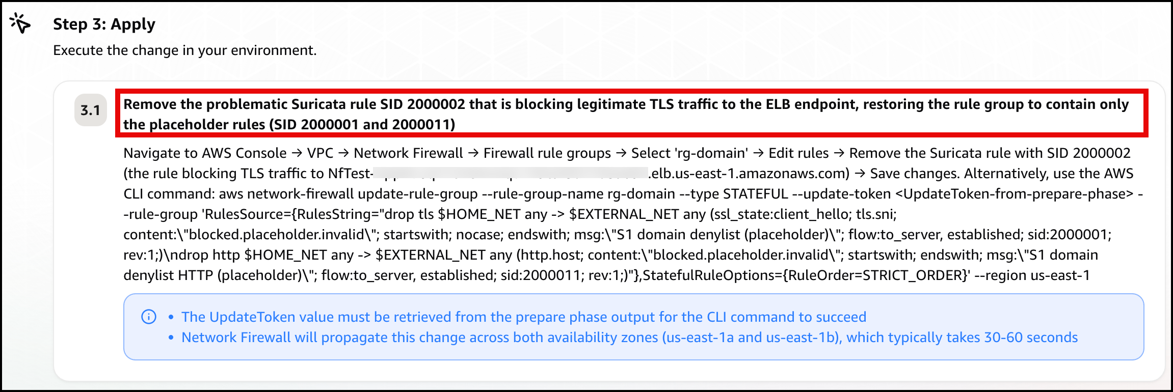
Finally, the agent presents a mitigation plan, recommending you remove the problematic deny rule (SID 2000002) to restore connectivity (Figure 6).
Figure 6: Scenario 1 – The mitigation plan
Note: In a real-world environment, this type of rule typically exists for a reason. Before removing it, verify whether it was intentional but scoped too broadly. If so, refine the rule to block only unauthorized endpoints rather than removing it entirely.
Confirm recovery. Apply the change the agent recommends. After the deny entry is gone, DroppedPackets falls back to baseline, Alarm-1 clears, and the card returns to green. Move on to Scenario 2.
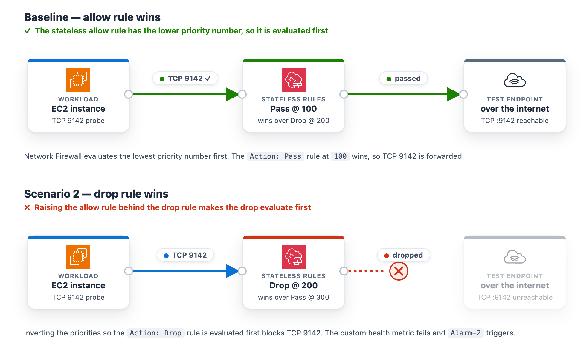
At baseline, the rg-stateless-priority stateless rule group keeps the allow rule at priority 100 and the drop rule at 200 for the test class, TCP destination port 9142. The workload opens a TCP connection to the test endpoint on this port. Lower priority numbers evaluate first, so the allow rule wins. This scenario uses port 9142 instead of 443 to demonstrate a stateless rule, which matches on the packet’s 5-tuple (protocol, ports, addresses) rather than application content.
Introduce the change. Invert the two rule priorities so the drop rule evaluates before the allow rule. This is the kind of change a rushed rule edit can introduce.
In the navigation pane, under Network Firewall, choose Network Firewall rule groups.
Choose the rg-stateless-priority rule group to open its details page.
In the Rules section, choose Edit.
Raise the (Action: Pass) rule’s priority number so it sits after the (Action: Drop) rule, then choose Save. For example, change the (Action: Pass) rule from 100 to 300 (any number higher than the drop rule’s 200 works). You only need to move one rule, and using 300 avoids a clash with the drop rule that already sits at 200. Network Firewall evaluates the lowest priority number first, so the (Action: Drop) rule at 200 now wins for this traffic class, ahead of the (Action: Pass) rule at 300.
Figure 7: Scenario 2 – Rule priority change blocking the traffic class
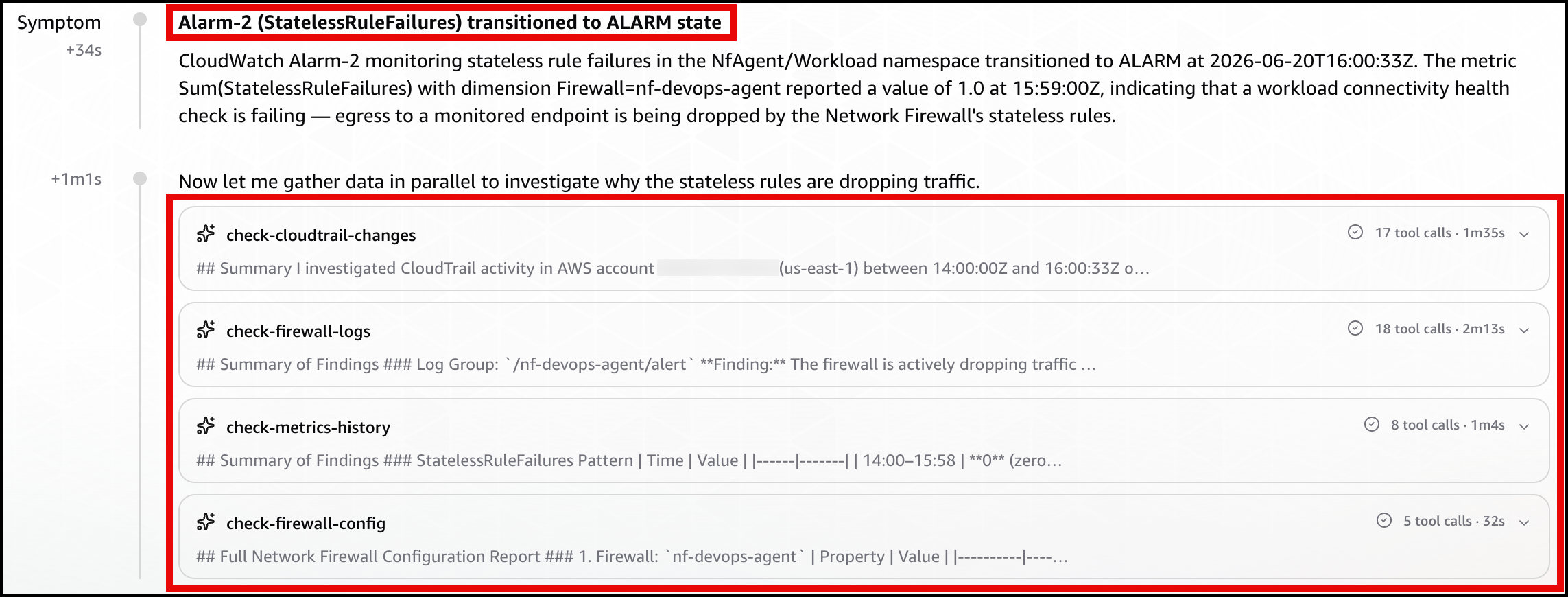
What happens. The drop rule now wins, the TCP connection to the test endpoint on port 9142 times out, the StatelessRuleFailures metric climbs above baseline, and Alarm-2 moves to ALARM. The Scenario 2 card reads DROPPED (with the condition Stateless rules dropping the monitored traffic class), while the Scenario 1 and Scenario 3 cards stay Healthy (Figure 8). On the topology, the alarm pipeline from CloudWatch through Amazon SNS and Lambda to DevOps Agent and the workload-to-firewall inspect lines both turn amber, which the legend defines as collateral / alarm active, because the packets are now dropped at the firewall. To demonstrate the resulting failure, the TLS :9142 line from the internet gateway to the test endpoint is shown in red, which the legend defines as dropped (root cause).
Figure 8: Scenario 2 active
Let DevOps Agent investigate. A stateless drop happens before traffic reaches the stateful inspection engine, so it produces no ALERT log entries. The agent turns to configuration and flow logs instead:
Reads the stateless rule group state and finds the drop rule at the lower priority number, ahead of the pass rule, so the drop evaluates first.
Reads the flow logs and sees passed packets drop to zero within a minute of the change.
Searches CloudTrail and surfaces the UpdateRuleGroup call that inverted the priorities, identifying the user, role, and timestamp about a minute before the alarm.
Reports the root cause as that priority inversion. Recommends removing the redundant drop rule and managing the rule group through infrastructure-as-code (IaC) to prevent manual misconfigurations.
Presents this as a plan you review and apply, not an automatic change.
In the DevOps Agent Operator Web App view, the agent first restates the Alarm-2 trigger and confirms that a workload connectivity health check is failing because the firewall’s stateless rules are dropping egress (Figure 9).
Figure 9: Scenario 2 – The symptom
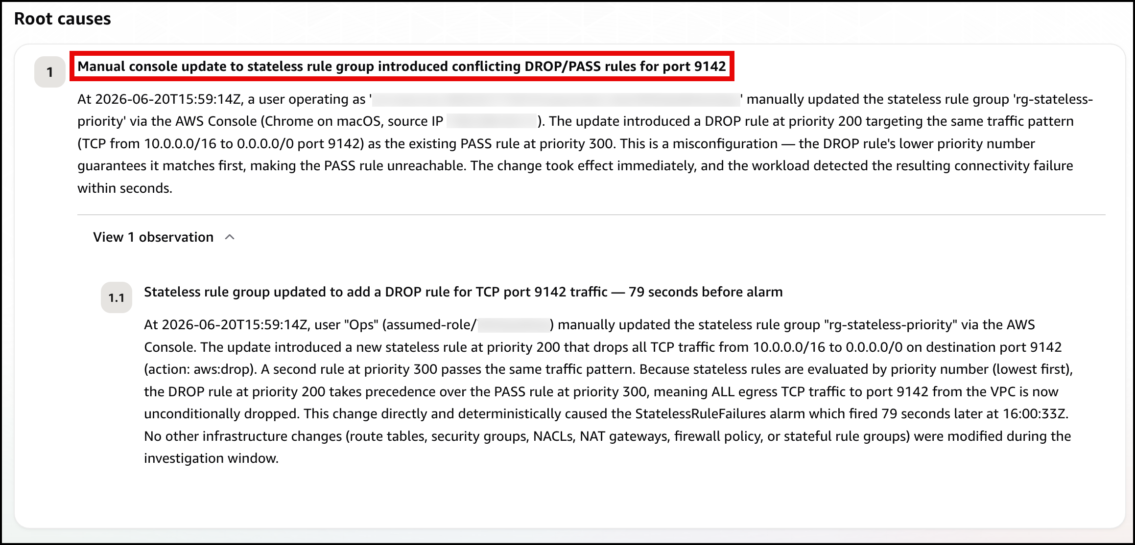
Next, the agent identifies the root cause, using the rule-group state and CloudTrail to pinpoint the conflicting DROP/PASS rules, where the new DROP rule’s lower priority number makes it match first (Figure 10).
Figure 10: Scenario 2 – The root cause
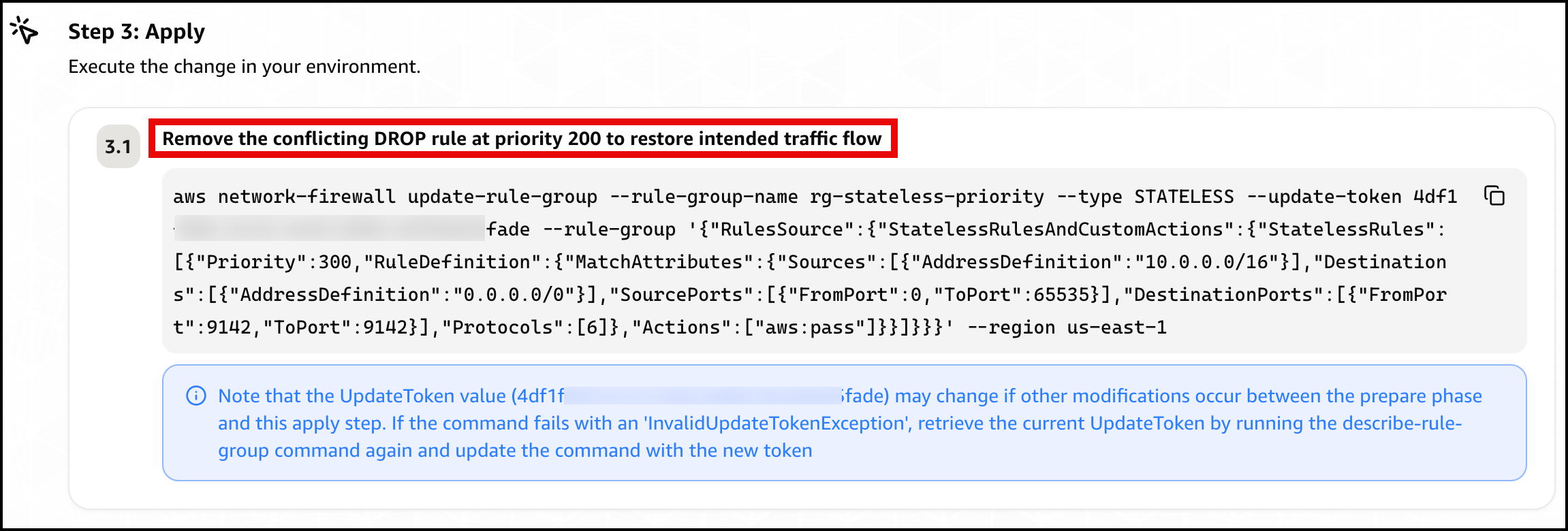
Finally, the agent presents a mitigation plan, recommending you remove the conflicting DROP rule at priority 200 to restore traffic flow (Figure 11).
Figure 11: Scenario 2 – The mitigation plan
Confirm recovery. Apply the change the agent recommends. After the allow rule is ahead of the drop rule again, Alarm-2 clears and the card returns to green. Move on to Scenario 3.
Scenario 3. Asymmetric cross Availability Zone routing drop
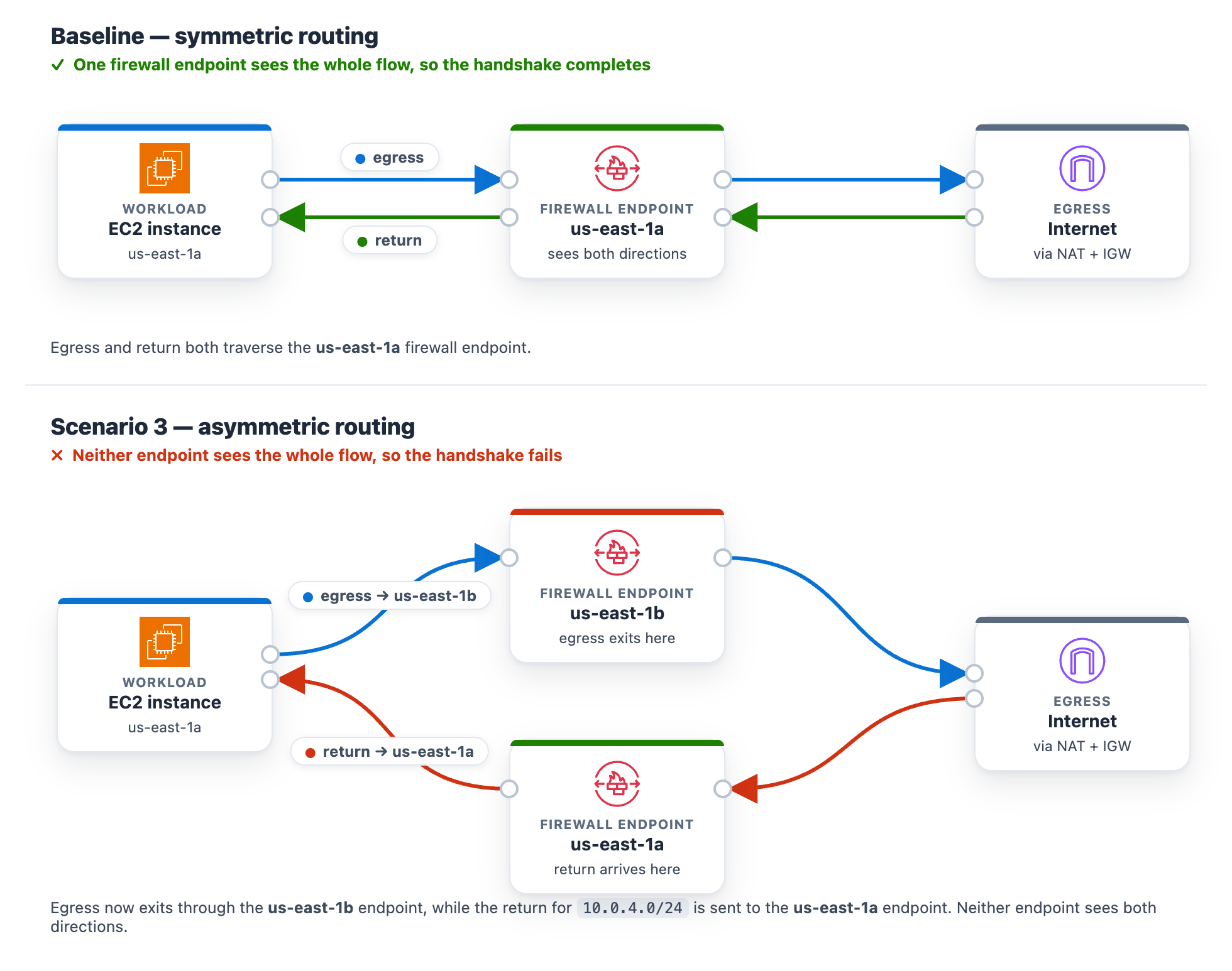
At baseline, the protected subnet in each Availability Zone routes its egress through the firewall endpoint in that same Availability Zone , and the matching return route uses that same endpoint. One endpoint sees both directions of the flow, so the stateful engine completes the handshake. The workload runs in the protected subnet in us-east-1a (CIDR 10.0.4.0/24), so at baseline its egress and its return both use the us-east-1a firewall endpoint.
Introduce the change. Make the flow asymmetric by sending egress out one Availability Zone endpoint while the return comes back through the other. This takes two route edits, and both are required. With only the first edit the flow can still complete, so the alarm will not trigger until both are saved. It makes no firewall-policy change, mirroring a real multi-Availability-Zone routing mistake.
To create asymmetric cross Availability Zone routing
Go to the Amazon VPC console and choose Route tables in the navigation pane.
Flip the egress. Select the NfNetworkStack/SampleVpc/protectedSubnet1 route table (the us-east-1a protected subnet, where the workload runs). On the Routes tab, choose Edit routes. Its 0.0.0.0/0 route currently targets the us-east-1a firewall endpoint. For the target, choose Gateway Load Balancer Endpoint and select the us-east-1b firewall endpoint, then choose Save changes.
Move the return. Select the NfNetworkStack/SampleVpc/publicSubnet2 route table (the us-east-1b public subnet, where egress now exits). Choose Edit routes, then Add route. For the destination enter the workload CIDR 10.0.4.0/24. For the target, choose Gateway Load Balancer Endpoint and select the us-east-1a firewall endpoint. Choose Save changes.
After both edits, a flow’s egress leaves through the us-east-1b endpoint while its return is directed to the us-east-1a endpoint. Neither endpoint sees the whole flow.
Figure 12: Scenario 3 routing change breaking the flow’s symmetry
What happens. A new connection leaves through one endpoint. Its return arrives at the other endpoint, which never saw the connection open, so the handshake fails. Unlike Scenarios 1 and 2, this affects the whole subnet, so all egress stops and Alarm-2 and Alarm-3 both move to ALARM. The AWS/NetworkFirewall DroppedPackets alarm (Alarm-1) stays quiet because no endpoint is making a drop decision. The flow is lost to asymmetric routing rather than counted as a firewall drop. This is why monitoring application connectivity matters. A routing fault is invisible to the firewall’s own drop counter. On the status page, the Scenario 2 card reads DROPPED (with the condition “Stateless rules dropping the monitored traffic class”) and the Scenario 3 card reads DROPPED (with the condition Return traffic dropped by asymmetric cross-Availability-Zone routing), while the Scenario 1 card stays Healthy (Figure 13). On the topology, the alarm pipeline from CloudWatch through Amazon SNS and Lambda to DevOps Agent and the workload-to-firewall inspect lines both turn amber, which the legend defines as collateral / alarm active, while the egress path from the firewall through the NAT gateway and the TLS :9142 and HTTPS · routing lines to the test endpoint turn red, which the legend defines as dropped (root cause).
Figure 13: Scenario 3 – The status page during a path-wide outage
Let DevOps Agent investigate. Both Alarm-2 and Alarm-3 fire in the same datapoint. DevOps Agent recognizes them as linked and merges them into a single investigation:
Reads the flow logs and sees bidirectional TLS connections stop abruptly, with only one-way traffic remaining and no flows reaching the established state.
Reads the firewall metrics and sees received and passed packets shift from one Availability Zone to the other at the moment of the change.
Calls DescribeRouteTables and finds the egress route pointing at one Availability Zone firewall endpoint while the return route points at the other.
Searches CloudTrail and surfaces the ReplaceRoute and CreateRoute calls by the same user, about a minute before both alarms fired.
Reports the root cause as that asymmetric routing change. Recommends restoring symmetric same-Availability-Zone routing so egress and return traverse the same endpoint.
Presents this as a plan you review and apply, not an automatic change.
A mitigation plan is a recommendation you review, not an automatic change, and the right fix depends on the intended design. Restoring symmetric routing can mean sending the workload subnet’s egress back through its own-Availability-Zone firewall endpoint (this sample’s architecture) or, in a design that doesn’t inspect this path, back through a NAT gateway. The agent infers a plausible target from what it can observe, so review the specific route it proposes against your intended topology before you apply it. (Connecting your pipeline or infrastructure-as-code, covered in the next section, lets the agent recommend the target that matches your design.)
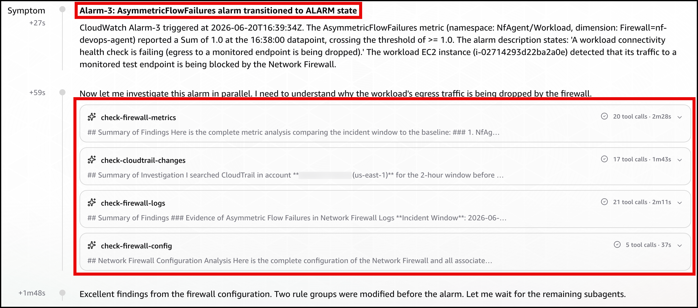
In the DevOps Agent Operator Web App view, the agent restates the Alarm-3 (AsymmetricFlowFailures) trigger and confirms the workload’s egress to a monitored endpoint is being blocked by the Network Firewall (Figure 14).
Figure 14: Scenario 3 – The symptom
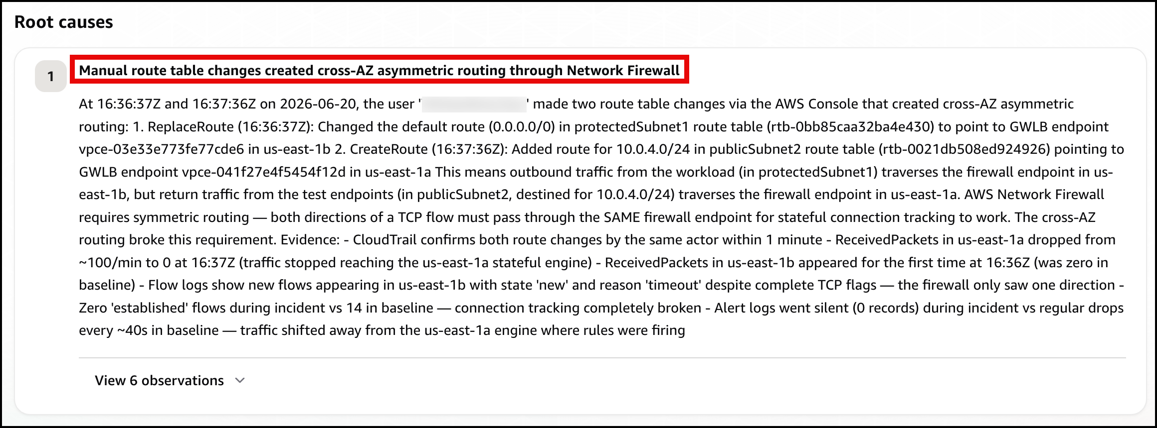
Next, the agent identifies the root cause: manual route table changes that created cross-AZ asymmetric routing through the network firewall, breaking its symmetric routing requirement (Figure 15)
Figure 15: Scenario 3 – The root cause
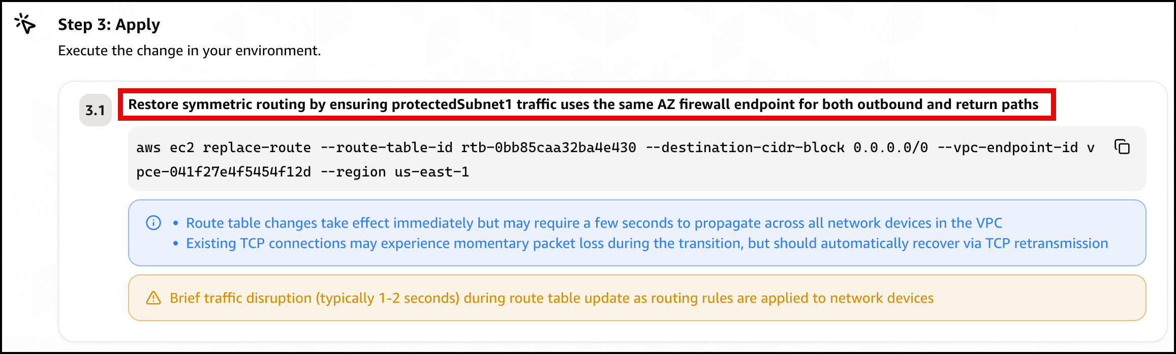
Finally, the agent presents a mitigation plan, recommending you restore symmetric routing by pointing protectedSubnet1‘s default route back to the same Availability Zone firewall endpoint, so one endpoint sees both directions of the flow again (Figure 16).
Figure 16: Scenario 3 – The mitigation plan
Confirm recovery. Apply the change the agent recommends, after checking the route target matches your intended design. After the workload subnet’s egress and return use the same Availability Zone firewall endpoint again, the control probe recovers, the alarms clear, and every card returns to green.
Further considerations
In production a single change can trigger several alarms at the same time, as Scenario 3 shows. DevOps Agent links related investigations and works them as one, so you review a single root cause. You can validate the linked findings or unlink an alarm to investigate it independently. If you would rather collapse alarms before they reach the agent, you can add correlation logic in the bridge Lambda function, buffering and grouping by firewall. You can also add email, Amazon Simple Queue Service (Amazon SQS), or HTTP subscribers to the SNS topic, or add the webhook Lambda function to a topic you already run. DevOps Agent produces a mitigation plan but does not change your environment on its own.
You can also give the agent more to work with. DevOps Agent connects to source repositories and CI/CD pipelines, integrating with GitHub (including GitHub Enterprise Server and GitLab Self-Managed through a private connection). It can associate AWS resources with deployments of AWS CloudFormation, AWS CDK, Amazon Elastic Container Registry (Amazon ECR) images, and Terraform. With deployed configuration and recent deployment events in view, the agent correlates the disruption against the change that introduced it and recommends a fix matching your intended design. For this sample, that means recommending the workload subnet’s own Availability Zone firewall endpoint rather than a generic symmetric path.
DevOps Agent also supports proactive incident prevention. It analyzes patterns across past investigations and delivers recommendations to prevent similar issues from recurring, including governance recommendations that strengthen deployment processes and pipeline controls. For Network Firewall rule changes, this means the agent can recommend guardrails for your CI/CD pipeline based on the classes of misconfigurations it has already resolved. You can access these recommendations through the Improvements page in the DevOps Agent Operator Web App.
Clean up
Clean up the environment with one command.
bash scripts/destroy.sh
It reverts any active scenario, runs cdk destroy for all stacks, and sweeps for stragglers by the Project = nf-devops-agent tag. The main cost drivers are the two Network Firewall endpoints, the NAT gateways (one in the main VPC for each Availability Zone, one in the test-endpoint VPC), and the test endpoint’s load balancers. Each of these bills at an hourly rate for as long as it’s provisioned, whether or not traffic is flowing, so a stack left running continues to accrue charges around the clock even while idle. Running the scenarios and tearing the stack down the same day limits the cost to a few active hours rather than days of idle hourly charges.
Conclusion
In this post, we showed you how AWS DevOps Agent accelerates troubleshooting for three common network firewall connectivity issues. The first was a domain deny list. The second was a stateless priority inversion. The third was an asymmetric cross-AZ routing drop. For each one, DevOps Agent investigated the drop and returned a root cause with a mitigation plan you approve before applying. The first scenario triggered on a prebuilt Network Firewall metric, and the other two on application health metrics. That shows both ways to alarm on a firewall problem through one pipeline.
Border Gateway Protocol (BGP) is the de facto routing protocol of the Internet. It offers built-in mechanisms to allow entities, represented by Autonomous Systems (ASes), to express how they want to send and receive traffic on the Internet. One such mechanism is path attributes, which carry essential routing information and metadata for their associated route. The path selection algorithm processes some of these path attributes in a deterministic sequence to calculate the best path for this specific prefix.
Using our unique position on the Internet, we took an investigative look at one of the well-known mandatory attributes in BGP, the ORIGIN attribute. ORIGIN must be present in every BGP prefix announcement and should not be modified by any router after being set by the originating one. What we found through our own experiments was a dramatic ~70% of observed paths in numerous vantage points have a different ORIGIN value compared to what was set by the originating Autonomous System. This ORIGIN attribute manipulation has a significant impact on the way traffic is forwarded on the Internet, as we’ll explore in this post.
BGP ORIGIN and its operational history
The ORIGIN attribute indicates how a route was injected into BGP — not to be confused with the origin AS that indicates whichASannounced a route. It has three possible values:
(0) IGP: Indicates the route is interior to the originating AS
(1) EGP: A historical value indicating that the route was learned via the old Exterior Gateway Protocol (EGP), which is obsolete and not intended to be used in the modern Internet
(2) INCOMPLETE: Indicates the route was learned via an unknown or external source
Among total observable routes from all the public BGP collectors of RIPE RIS and RouteViews, 89.8% have ORIGIN set to IGP, 3.5% to EGP, and 6.7% are INCOMPLETE. As mentioned above, EGP is meant to be deprecated entirely and INCOMPLETE carries a minority share of total routes. These figures suggest that while IGP is by far the most popular value for ORIGIN, more than 10% of routes have an EGP or INCOMPLETE value that could make a difference in routing decisions.
As a part of the BGP path selection process, a router evaluates the ORIGIN if two routes have equal Local Preference and AS_PATH length, selecting and installing the path with the lower ORIGIN value.
The ORIGIN attribute is generated by the speaker that originates the associated routing information. Its value SHOULD NOT be changed by any other speaker.
Though the guidance is to not modify the ORIGIN attribute, due to its early evaluation in the route selection process, this attribute has presented an attractive option for ASes to alter route preferences and divert traffic either through or away from their networks.
For example, in the diagram below, AS64501 announces a prefix with ORIGIN set to INCOMPLETE and propagates this announcement to both of its customers, AS64502 and AS64503. Normally, both of them should prepend their own AS in the AS_PATH and forward the announcement to their common customer AS64504, preserving the INCOMPLETE value. However, to increase the likelihood of their route being selected over competitors’, AS64503 modifies the ORIGIN to IGP. As a result, AS64504 receives two routes for the prefix with equal AS_PATH lengths, but the one from AS64503 carries the preferred IGP value. Thus, AS64504 will select the route through AS64503 to send traffic to AS64501, driving more traffic and revenue to that provider.
This simple change, to an inaccurate but more preferable ORIGIN, allows the transit provider to draw traffic and profit.
The network operators community has silently accepted the reality that transit providers have been rewriting the ORIGIN attribute to IGP in order to attract more traffic to their links. However, James Bensley at the RIPE 91 meeting was the first to spotlight the widespread adoption of this manipulation technique by major networks. A follow-up presentation by Celsa Sánchez at the LACNIC 45 meeting investigated the impact of this behavior in the LACNIC (Latin American and Caribbean) region. While a public disclosure should discourage this practice, it highlights the reality that route selection is a revenue-driven arms race. Rather than waiting for competitors to resume RFC compliance, network operators are more likely to quickly resort to rewriting the ORIGIN simply to level the playing field.
This increasingly inconsistent handling of ORIGIN across the Internet prompted the creation of a now-expired Internet-Draft that recommended its deprecation. To uncover the extent of this phenomenon and track its actors along with their intentions, we conducted our own experiments and share the results in the next section.
ORIGIN attribute manipulation analysis
In our experiment, we announced three IPv4 and three IPv6 prefixes, each with a different ORIGIN value (IGP/EGP/INCOMPLETE) from all of our peering locations using BGP Anycast. After confirming global propagation, we later withdrew the prefixes to trigger the path hunting process, revealing more paths to the test prefixes, giving us more opportunities to spot altered ORIGINs. As shown in the figure below, we used the BGPKIT toolkit to parse the Update messages from the Multi-threaded Routing Toolkit (MRT) dumps of all the public BGP collectors from RIPE RIS and RouteViews, and the local BMP data that we collect from our border routers. Note that we opted to analyze the Updates instead of the Routing Information Base (RIB) dumps, which are snapshots of the routing tables of the peer ASes, to retrieve as many as possible routes both during the announcement and the withdrawal phase.
A fundamental difficulty of BGP analysis is the lack of visibility into all ASes on the Internet for a single routing announcement. This gap is widened by the modern flattening of the Internet, driven by hyperscalers and CDNs bypassing traditional transit routes in favor of direct, local peering. Consequently, public monitors miss a significant portion of the BGP topology for a given prefix, meaning inferences about AS properties always carry inherent uncertainty.
Finding ORIGIN rewriters in two-hop AS_PATHs
First, we focused on AS_PATHs with only two ASes: “ASX AS13335”, where we call ASX a direct peer. Since we configured our routers to propagate our announcements with a specific ORIGIN, we are confident that if we observe a different ORIGIN, ASX must have changed it to its new value. The table below shows the manipulation behavior of the 352 direct peers for IPv4 where the “Advertised ORIGIN” column shows what value is being advertised for each of our three prefixes, and the right-hand side columns list the ORIGIN values observed by direct peer ASes:
We would like to point out two interesting observations. First, three ASes change the ORIGIN to EGP, and four ASes change it to INCOMPLETE, regardless of its original value, meaning that they are potentially attempting to deprioritize these routes. We reached out to one of these ASes’ network engineers and confirmed that they are rewriting the ORIGIN to EGP on routes received from peers or providers (to render them less preferred compared to customers’ routes). Second, for the non-IGP prefixes, three ASes propagate routes with both the original value and IGP (the two right-most columns above). Based on other attributes of the routes such as communities and AGGREGATOR, we infer that these ASes receive our routes at multiple peering locations and update the ORIGIN to IGP, presumably to forward traffic through a preferred point. Combining the latter ASes with the ones consistently rewriting to IGP, we discover that almost 10% of the direct peers change the ORIGIN attribute to IGP.
In testing IPv6, we expected similar results but wanted to note discrepancies involving the manipulation of the ORIGIN value by the same AS between two address families. In the following table we present the manipulation behavior of the 315 direct peers for IPv6:
Most noteworthy is that two direct peers change the ORIGIN to IGP only for IPv4 prefixes and not IPv6, implying different configurations for the two address families.
Narrowing our analysis to the Tier-1 ASes, six out of the 16 appear to manipulate the ORIGIN value to IGP, matching the results of the previous study. Note that through manual investigation we found that one Tier-1 network changes the ORIGIN value to IGP for routes learned from peers, while it preserves it for customer routes. This pattern of behavior across several Tier-1 networks reflects the drive to attract the most traffic and cancel out other ORIGIN modifiers’ advantage.
Identifying rewriters in longer AS_PATHs
Based on these initial results, we extended our methodology to process longer paths and infer the behavior of more ASes. Briefly, our algorithm works as follows:
We seed our trusted set (T) with AS13335. T holds all the ASes that preserve the ORIGIN.
For each AS_PATH:
Filter out all ASes in T.
If only one AS remains, we can attribute the ORIGIN to that AS. We record the mapping AS → ORIGIN(s).
For each pair AS → ORIGIN(s):
If ORIGIN(s) == original value, we add AS to T.
Else, we add AS to M(odifiers).
If T was updated in 3, repeat the procedure from 2.
Applied to the routes of our IPv4 and IPv6 prefixes originated with EGP and INCOMPLETE, this methodology increases our AS attribution to 606 out of 802 (75.6%) visible ASes in the AS_PATHs, out of which 64 (10.6%) are changing the ORIGIN to IGP. Motivated by the Tier-1s adopting this technique, we studied the significance of the attributed ASes using CAIDA’s AS Rank. AS Rank provides a ranking of the ASes based on their customer cone (i.e., themselves and all the ASes that can be reached through provider-customer links).
In the figure below, we show the cumulative distribution (CDF) of AS Ranks of the attributed ASes. An interesting observation is that the IGP-rewriting ASes are highly concentrated at the top of the AS hierarchy, with 20.3% of the rewriting ASes falling in the top-50 of AS Rank.
Impact of large ASes rewriting ORIGIN
In total, 26% of the top 50 ASes and 20% of the top 100 ASes are manipulating the ORIGIN attribute, highlighting that despite their overall low percentage, the ASes resetting the ORIGIN are highly central and impactful on the Internet.
The impact is further reinforced by the finding that a staggering 70% of the unique IPv4 AS_PATHs and 67% of IPv6 AS_PATHs observed in the experiment have ORIGIN reset to IGP. We also studied the changes imposed on best path selection by consolidating BGP Updates to compute the converged active routing-table state of each peer AS. We used the prefix advertisement with ORIGIN set to IGP as a control group to compare AS_PATHs observed versus our EGP and INCOMPLETE announcements. When doing so, we found in IPv4 that 110 AS_PATHs out of the total 539 (20%) traversed Tier-1 networks and that resetting the ORIGIN to IGP secured for ORIGIN rewriters 12 additional paths (an increase of 18%) that would otherwise go through the networks that preserve ORIGIN. The effect is even stronger in IPv6, where the rewriters gained 33 more paths (40%). These include 11 paths that for our control group did not traverse any Tier-1 network. This highlights the redirection of traffic toward large Tier-1 ISPs when the ORIGIN was manipulated, diverting traffic away from alternative ISPs.
As you can see, Internet routing is significantly impacted by the manipulation of the ORIGIN attribute. In our experiments, we can easily observe the effects on BGP path selection and demonstrate how rewriting ORIGIN is a way to siphon traffic and generate revenue. There is no valid technical reason to require a rewrite of the ORIGIN attribute, and we can see it does not make sense to depend on ORIGIN as a driving factor in deciding what routes to take.
Deprecating the ORIGIN attribute
Given our findings of widespread ORIGIN manipulation, we have to ask ourselves whether this attribute has a meaningful role at all in the modern Internet. We think the answer is No.
The inconsistent treatment of ORIGIN creates unfairness between networks opportunistically changing it and networks complying with the RFC. While immediate deprecation of a mandatory attribute in BGP would be infeasible, there has already been work proposed in the IETF to make the ORIGIN attribute less relevant in BGP path selection. We believe requiring BGP (vendor) implementations to set ORIGIN as IGP on all routes received and advertised is a reasonable starting point. IGP is already set as ORIGIN on the great majority of routes.
We want to revive these conversations in the community and the IETF about the ORIGIN attribute and its future (or lack thereof) on the Internet. This may include renewing the expired draft “Scrubbing BGP ORIGIN Attribute” (draft-marenamat-idr-scrub-bgp-origin-00), or may include a new approach entirely. Internet routing would be better and fairer without the ORIGIN attribute carrying influence.
This batch of kernels includes a hefty set of updates, possibly the
the largest ever. 7.1.5-rc1,
for example, included more than 2,000 patches, 6.18.40-rc1
included 1,611 patches, and so forth. Users are advised to upgrade.
Registration is now
open for the 2026 Linux Plumbers Conference, to be held October 5
to 7 in Prague, Czechia. Tickets to this event tend to sell out
quickly, so interested attendees probably should not procrastinate.
AWS GlueData Catalog view is a multi-dialect view that supports querying from multiple SQL query engines, such as Amazon Athena, Amazon Redshift Spectrum, Apache Spark in Amazon EMR and AWS Glue. You can create a Data Catalog view in one account, using an AWS Identity and Access Management (IAM) definer role in the same or different account and use AWS Lake Formation to share the view across multiple accounts. The definer role has the required full SELECT on the base tables to create the view and share it with other users for querying. The Data Catalog assumes the definer role and manages access of the base tables when the view is queried, thus allowing to share a subset of data without sharing the underlying base tables.
AWS Glue now adds AWS SDK support for creating and updating the ATHENA dialect of Glue views. With this addition, you can now create ATHENA and SPARK dialects of Glue views simultaneously, using a cross account IAM definer role. This feature enhances the automation to create and update Glue views, like that of Data Catalog tables. In our earlier blog Create AWS Glue Data Catalog views using cross-account definer roles, we had introduced IAM definer roles in a cross-account use case to create Data Catalog views with SPARK dialects using the APIs – CreateTable() and UpdateTable() – while creating and adding ATHENA dialects using Athena query editor. As a continuation to it, this post shows you how to use the Catalog objects API CreateTable() to programmatically create ATHENA and SPARK dialects using cross-account IAM definer roles, and how to add the ATHENA dialect programmatically for the views that were created earlier with only SPARK dialect.
Cross account definer roles enable enterprise data mesh architectures where multiple accounts are interconnected in a central governance and multiple producers and consumers. The central governance account hosts the database, tables and permissions, while the producer accounts maintain CI/CD pipelines to create and manage those data assets. Having the definer role in producer accounts allows those CI/CD pipelines to be fully managed by IAM roles in the individual accounts.
Key points on creating multi-dialect views using cross-account definer roles
ATHENA dialects are validated and asynchronously created. Hence, a cross-account Glue connection is required for validation for every producer account-central governance account pair. This is a one-time setup.
SPARK dialects are not validated. Hence SPARK dialect’s create syntax requires SubObjects list of the base tables and StorageDescriptor fields for the columns of the view.
Though queries on cross account views can be run using database resource link names, the view definition SQL query for creating the view requires the original database and base table names from the central governance account.
If a view has SPARK and ATHENA dialects available, we recommend updating both the dialects of the view simultaneously using update_table() API/SDK, for any changes in the SQL definition of the view or the base table. This will keep both the dialects queryable.
Creating and updating both SPARK and ATHENA dialects using cross account definer role is supported using AWS CloudFormation.
The Data Catalog view that can be created using cross account IAM definer roles are available in SPARK and ATHENA dialects and currently not supported for Redshift Spectrum dialect.
Prerequisites
We use the same setup used in Create AWS Glue Data Catalog views using cross-account definer roles for the sample database, tables, definer role, resource link, IAM and Lake Formation permissions on those resources and principals between the two AWS accounts. Summarizing the requirements as below.
The setup includes a central governance account with Data Catalog database bankdata_icebergdb and two tables transaction_table1 and transaction_table2, a producer account with a Data-Analyst role used as view definer role.
Lake Formation permissions on the central account’s database and tables are granted to the producer account Data-Analyst role as per the earlier blog. The definer role in producer account should have database DESCRIBE and CREATE_TABLE permissions, table SELECT and DESCRIBE permission on all columns and rows of the base tables. The IAM permissions required on the definer role are detailed in Prerequisites for creating views. Similarly, follow the earlier blog to create resource link for the shared database and grant Lake Formation permissions on the resource link to the Data-Analyst
An Athena data source named centraladmin in the producer account, pointing to the Data Catalog of the central governance account.
Creating ATHENA and SPARK dialects at the same time
Creating both ATHENA and SPARK dialects of a Glue catalog view simultaneously is now supported by the AWS SDK. In the producer account, create a new Glue connection, required for the Athena dialect validation. This is a prerequisite for creating the ATHENA dialect of the Glue catalog view using cross account definer role. Then we create a Glue view with both dialects.
Sign in to the producer account as the Lake Formation admin role, or any role with permission to create AWS Glue connections.
Note: If you are using Athena for the first time in your account or using Primary workgroup, setup the query results location bucket using Specify a query result location.
Sign out as the Lake Formation admin and sign back in to the producer account as the definer IAM role, Data-Analyst.
Create an AWS Glue view using the create-table CLI command and JSON file, or using the AWS SDK for Python (Boto3) script.
The content of create_multipledialects.json is as follows.
 {
   "DatabaseName": "rl_bank_iceberg",
   "TableInput": {
     "Name": "view_2dialects_2basetables_fromcli",
     "StorageDescriptor": {
       "Columns": [
         {
           "Name": "transaction_id",
           "Type": "string"
         },
         {
           "Name": "transaction_type",
           "Type": "string"
         },
         {
           "Name": "transaction_amount",
           "Type": "double"
         },
         {
           "Name": "transaction_location",
           "Type": "string"
         },
         {
           "Name": "transaction_date",
           "Type": "date"
         }
     },
     "ViewDefinition": {
       "SubObjects": [
         "arn:aws:glue:us-west-2:<central-account-id>:table/bankdata_icebergdb/transaction_table1",
         "arn:aws:glue:us-west-2:<central-account-id>:table/bankdata_icebergdb/transaction_table2"
        ],
       "IsProtected": true,
       "Representations": [
         {
           "Dialect": "SPARK",
           "DialectVersion": "1.0",
           "ViewOriginalText": "SELECT a.transaction_id, a.transaction_type, a.transaction_amount, b.transaction_location, b.transaction_date FROM bankdata_icebergdb.transaction_table1 a RIGHT JOIN bankdata_icebergdb.transaction_table2 b ON a.transaction_id = b.transaction_id",
           "ViewExpandedText": "SELECT a.transaction_id, a.transaction_type, a.transaction_amount, b.transaction_location, b.transaction_date FROM bankdata_icebergdb.transaction_table1 a RIGHT JOIN bankdata_icebergdb.transaction_table2 b ON a.transaction_id = b.transaction_id"
         },
         {
            "Dialect": "ATHENA",
            "DialectVersion": "3",
            "ViewOriginalText": "SELECT a.transaction_id, a.transaction_type, a.transaction_amount, b.transaction_location, b.transaction_date FROM bankdata_icebergdb.transaction_table1 a RIGHT JOIN bankdata_icebergdb.transaction_table2 b ON a.transaction_id = b.transaction_id",
            "ValidationConnection": "glue-view-validation-connection"
         }
       ]
     }
   }
}
Notes about fields in the above CLI input JSON (applies to all SDK):
The definer is by default the API caller, but a Definer field can be set to explicitly specify a different IAM role.
In the ViewDefinition, database qualifiers are required for SPARK dialect. That is, the SQL definition provided for ViewOriginalText and ViewExpandedText should be in <source_database_name>.<source_table_name> format.
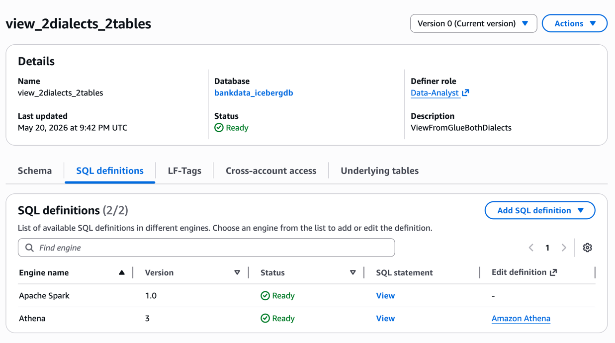
After the view is created, you can inspect the details on the Lake Formation console. The SQL definitions show both ATHENA and SPARK as shown in the following screenshot.
If your view creation fails for any of the dialects, you can use the AWS Glue get-table CLI command with --include-status-details to see what the error is and rectify it.
The PySpark script for creating a view with ATHENA and SPARK dialects are provided below. Download and edit the Pyspark script with your bucket name, producer and central account ids, region and relevant Glue resource names: bdb_5773_createview_bothdialects.py
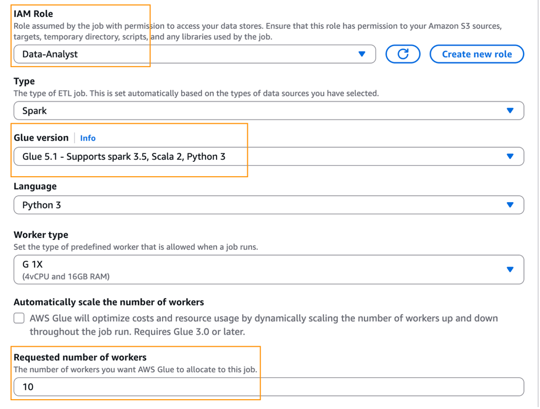
Provide the following settings to run the script in your Glue Studio. For details on running a Spark job in Glue, refer Working with Spark jobs in AWS Glue.
Choose Data-Analyst as the job execution IAM role.
Choose Glue 5.1 for Glue version.
For the Requested number of workers, provide >=4. This is an FGAC Spark driver requirement, which is needed for Glue catalog views. Below screenshot shows these settings.
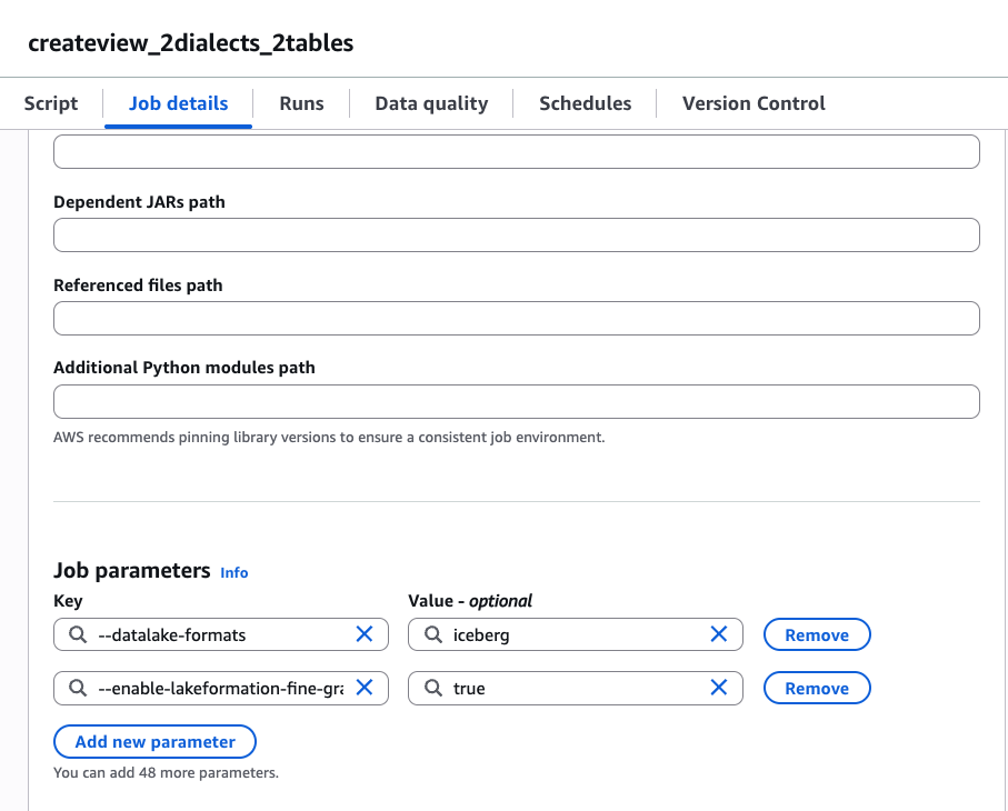
Add the following 2 properties as additional job parameters. A screenshot is shown for reference.
Adding ATHENA dialect using SDK to an existing AWS Glue view
You can update an existing AWS Glue view that was created with the SPARK dialect and add the ATHENA dialect using the SDK. The following example uses the update-table CLI command.
The content of add-athena-dialect.json is as follows.
{
    "DatabaseName": "rl_bank_iceberg",
    "ViewUpdateAction": "ADD",
    "TableInput": {
        "Name": "view_sparkfirst_athenanext",
        "ViewDefinition": {
            "Representations": [
                {
                    "Dialect": "ATHENA",
                    "DialectVersion": "3",
                    "ViewOriginalText": "SELECT a.transaction_id, a.transaction_type, a.transaction_amount, b.transaction_location, b.transaction_date FROM bankdata_icebergdb.transaction_table1 a RIGHT JOIN bankdata_icebergdb.transaction_table2 b ON a.transaction_id = b.transaction_id",
                    "ValidationConnection": "glue-view-validation-connection"
                }
            ]
        }
    }
}
Verify the added dialect on the view by reviewing the SQL definitions of the view in Lake Formation console or using GetTable(). If you want to edit the SQL definition or change the base tables of an existing view that has both SPARK and ATHENA dialects, you can do so using the update_table API (using SDK or CLI), with "ViewUpdateAction": “REPLACE” and provide both the dialect definition under ViewDefinition.
You can run queries on the view from the producer account as Data-Analyst. The view can be shared using Lake Formation Tags or named method, just like sharing tables, to additional consumer accounts from the central governance account. The consumer accounts will create a resource link and query the views.
Cleanup
To avoid incurring ongoing costs, clean up the resources you used for this post:
Revoke the Lake Formation permissions granted to the Data-Analyst role and the producer account from the central governance account.
Drop the Data Catalog tables, views, and the database.
Delete the Athena query results from your Amazon Simple Storage Service (Amazon S3) bucket.
Delete the Data-Analyst role from IAM.
Delete the AWS Glue connection and the Athena data source.
Delete the AWS Glue job, if you tried the Python script as an AWS Glue job.
Conclusion
In this post, I demonstrated how to use cross-account IAM definer roles with AWS Glue Data Catalog views, how to create and update ATHENA and SPARK dialects using the Data Catalog CreateTable() and UpdateTable() APIs. The multi-dialect Data Catalog views allow sharing a subset of data from different tables using Lake Formation permissions, including LF-Tags based access control. The cross-account definer roles support multi-account data mesh architectures so that the producer IAM roles can run the CI/CD pipelines in its account. We encourage you to try the feature and share your feedback in the comments.
Acknowledgements: I would like to thank all the team members who worked to add AWS SDK support for creating ATHENA and SPARK dialects together for AWS Glue views – Daniil Arushanov, Wyatt Hawes, Yuxi Wu, Santhosh Padmanabhan and Karthik Devaraj.
Fedora contributor Simon de Vlieger has published a blog
post with a walkthrough of how the project turns source code and
packages into the final release that users install on their systems.
It follows the a package from a packager’s git push to a composed
release: ISOs, cloud images, container images, and OSTree
deployments.
The walkthrough describes how the Fedora ‘sausage’ is created as of
Fedora 45, things change all the time; I hope to have time to update
this document every cycle or every few cycles of Fedora releases so
there’s both history and people can find up to date information.
Daniel Borkmann led a session at the 2026
Linux Filesystem, Memory-Management,
and BPF Summit about the progress that has been made with netkit, the subsystem
that allows virtual machines (VMs) running on Linux to perform networking efficiently.
When that did not fill the full time, he went on to discuss his idea for
using BPF to live-patch user-space applications. While netkit is making
progress, and can now support zero-copy receipt of packets into a VM in a
network namespace, the idea of using BPF for patching user-space programs
remains entirely speculative.
Providing a public, open way to browse the anonymous, aggregated
device data we collect was always part of the plan, and this preview
is our first step toward it.
You can already use it to search and filter devices to see
aggregated community insights, starting with a deliberately focused
set of specifics, such as whether a device requires an internet
connection, and which protocols and integrations it works with. We’ve
kept that initial scope narrow on purpose, giving us a solid
foundation we can build on together with you, our community, as the
database grows.
Президентът Тръмп даде сигнал, че е готов да задълбочи войната в Иран. Само преди месец писахме, че примирието между двете държави е подписано – днес това примирие не означава нищо, а още утре този бюлетин може би няма да е актуален. Политическото говорене на едро, заплахите, цинизмът и безсмислието са се превърнали в ежедневие. Министърът на войната Пийт Хегсет поиска 70 млрд. долара спешно военно финансиране след първите пет месеца от войната.
Хегсет обяви, че военните ще трябва да минават задължително изследване на нивата на тестостерон след 30-годишна възраст. Няма определени рамки какви нива на тестостерон ще се смятат за ниски, за да се изисква лечение – обичайно всяка лаборатория може да определя нива според методите си на изследване, което в допълнение се влияе и от препоръките на лекуващия лекар.
Решението на Хегсет идва в разгара на „тестостеронова мания“ в САЩ: рецептите за заместителна терапия с хормона са достигнали 12 млн. през 2025 г., ръст от 154% от 2020 г. насам. Онлайн клиники и търговци продават тестостерон като утвърдено лечение за мъже. Експерти обаче предупреждават, че по-високите нива на тестостерон нямат нищо общо с определени качества, които могат да направят един мъж „по-мъжествен“. Ако нивата на тестостерон по различни здравословни причини спаднат много под обичайните норми, последствията могат да бъдат умора, ниско либидо или загуба на мускулна маса, но при здрави мъже нивата на хормона нямат нищо общо с физическата сила.
Мъж с ниво на тестостерон около 700 нанограма на децилитър може да е точно толкова силен, колкото и мъж с 300 нанограма на децилитър. Нещо повече – нивата на тестостерон не са константа, а се променят в различните части на деня и според сезона, както и под влияние на други фактори. Терапията с тестостерон крие рискове: употребата на добавки може да понижи естествената способност на тялото да произвежда хормона, свивайки тестисите и намалявайки производството на сперматозоиди. Други ефекти са акне, оплешивяване и дори уголемяване на гърдите вследствие на преобразуването на част от приетия тестостерон в естроген.
Тестостеронът няма общо и с нивата на агресивност. Изследвания показват, че ако един мъж проявява агресия, причината обикновено е социална, а не хормонална. В проучване на 200 подрастващи момчета и родителите им екип, воден от Адам Станаланд, професор по психология в университета в Ричмънд, установява, че момчетата, реагиращи агресивно на стимули, които възприемат като „заплаха за мъжествеността“, са онези, които усещат силен социален натиск „да се държат като мъже“. Парадоксът е, че животът в армията – недостигът на сън, хроничният стрес, излагането на опасност и недоброто хранене, са изключително вредни за правилното функциониране на хормоните.
Всички тези научни факти обаче нямат значение във време, в което говорим за „криза на мъжествеността“ – с нея често се „борим“ с прояви на насилие и омраза към жени и към онези, които са приемани като „други“; с подлагане на хирургични интервенции в името на „по-мъжествено излъчване“; или чрез сформирането на групи и банди от вандали, често покрай бойни спортове.
По Америка ще познаете света.
Междувременно все повече жени в САЩ се тревожат какво ще се случи, ако имат дете, се посочва в статия в Women's Health. Жените посочват като основни притеснения здравния риск, следродилната депресия и пълното подчинение на майката на грижите за детето, както и финансовите трудности и състоянието на света като цяло.
В статията се казва още, че през неограничената информация в социалните мрежи хората често стигат до най-страшните истории за раждането, научават за възможно най-рисковите усложнения и чуват разкази на други родители, които изпитват съжаление, че имат деца, или се оплакват от липса на подкрепа от партньорите си. Експерти посочват, че повечето бременности в САЩ протичат без усложнения и че обществото трябва активно да работи в посока на подкрепа за майките.
Подкрепата за жените и майките не е сред трендовете в „мъжествените“ среди. Притесненията за демографията са.
По Америка ще познаете света.
Жителите на много държави по света вече гледат на Китай по-положително, отколкото на САЩ. Спадът в положителните възприятия започва около 2024 г., като в началото на втория мандат на президента Тръмп през 2025 г. 48% от отговорилите имат по-скоро добро отношение към Америка, а 38% – към Китай. Тази година числата са почти обърнати – 46% виждат Китай в по-добра светлина, а 36% избират САЩ.
На въпрос имат ли доверие, че държавата ще постъпи правилно по отношение на международната политика, положителното отношение към външнополитическото представяне на Китай е нараснало почти двойно от 2024 г. насам и е спаднало повече от двойно спрямо САЩ за същия период. Една от малкото сфери, в които САЩ все още държи висок рейтинг, е тази на свободните индивидуални права – повече хора отговарят, че САЩ уважават правата и свободите, което все още е обективна истина.
Фактът, че имам нужда да уточня „все още“, е показателен за състоянието на САЩ и на демократичния свят.
От една страна, бихме могли да кажем, че обръщането на САЩ към собствените им интереси би могло да става за сметка на други държави и на света като цяло, откъдето да идва негативното отношение към тях – това е и аргументът на много от консервативните симпатизанти на президента. Не съм съгласна обаче, че исторически САЩ никога не са гледали собствения си интерес; напротив, Америка е добре известна с арогантното си поведение на световната сцена.
В продължение на десетилетия обаче тя бе известна и с меката си дипломация, което направи от нея културен хегемон, а чрез културата рано или късно се печели всичко, както знаят добрите пропагандисти. Сега меката дипломация е заместена от друга пропаганда: на тестостерон, ритуален бой пред Белия дом и външна политика, характеризираща се с постоянството и деликатността на кисел попрезрял мъж (ако трябва да влезем в тона на (не)културния диалог).
Политиката на синтетичния тестостерон може да е много популярна сред определени сегменти от населението, но е абсурдна, смешна, глуповата и заради всичко това – дори ужасяваща за нормалните мислещи хора, които все още обитават средата между крайностите.
По-добрата позиция на Китай в общественото мнение надали се дължи на това, че изведнъж авторитарният комунизъм с капиталистически краски е станал атрактивна алтернатива на настоящия световен ред; в крайна сметка преди седмица книжари бяха извлачвани насилствено от книжарници в Хонг Конг.
Китай по някакъв начин е алтернатива на вакуума, отворил се от разпадналата се американска култура, точно толкова, колкото животът в Русия е алтернатива за недоволния български русофил. Обратното – разочарованието и липсата на нормалност блъскат общественото мнение към символа на Си Дзинпин – световен лидер, който, въпреки че също е зодия Близнаци (както впрочем и Румен Радев), може да се задържи на едно мнение и решение от сутринта до вечерта.
„Стабилността“ е онова, по което копнее средностатистическият човек, който не се интересува от сложните плетки на политиката, а просто иска да живее нормално. Който разбира копнежа по „стабилност“, разбира политиката. А ако това са само авторитарните лидери и режими, вината не е само тяхна.
Както и да е, по Америка ще познаете света.
На 14 юли губернаторката на щата Ню Йорк подписа мораториум върху изграждането на центрове за данни, който ще е в сила една година. Целта е през това време да се изучават ефектите на вече построените центрове за данни, за да може да се помисли за определени регулации. Тревогите на опонентите на мораториума се въртят около икономическите последствия, тъй като се страхуват, че меморандумът ще отблъсне инвеститорите. Според критиците на меморандума хората трябва да бъдат оставени сами да преценят дали искат центрове за данни в общностите си, или не.
По-умерените становища гласят, че политиките спрямо центровете за данни се третират само в контекста на развитието на изкуствения интелект и протестите срещу т.нар. интелектуален бълвоч (slop) – нискокачественото масово генерирано съдържание, което често цели бърза печалба или кликове. Инстинктивният и разумен аргумент е: защо трябва да хабим ценни ресурси, какъвто е водата, и да тормозим общностите с шум и замърсяване, за да подхранваме нещо, което не само ни затъпява, но и ни коства работни места?
Повечето хора обаче разчитат на ресурсите, които такава технология предлага – тя е толкова добра или лоша, колкото е ползвателят ѝ. Дали мораториумът ще е ефективен, ще покаже само времето. Въпросът е, че за разлика от България, дори в САЩ в криза все още се прави политика на действието – вземат се мерки, ефектите от тях се анализират и все пак някъде нещо се движи.
Дебатът за прогреса (най-вече технологичен) за сметка на толкова много други неща тепърва ще бъде актуален. През последните дни кабинетът на Тръмп активно премахва природозащитно законодателство, което ще позволи добив на петрол и други суровини от понастоящем защитени държавни земи.
Идеята за краткотрайна печалба и неспирен прогрес все още пречи да помислим как да живеем устойчиво в един все по-топъл и бедстващ свят, както виждаме и в България. Технологиите биха могли да помогнат и в тази посока – въпросът е кой и за какво ще ги използва.
По това, за което говори (и се кара) Америка, ще познаете онова, за което трябва да говори светът. Западна Европа току-що отчете най-горещия си юни някога.
Има и други новини. Тексаски пожарникар спасява три деца, заклещени под лодка, навръх 4 юли – националния празник на САЩ. Биотех стартъп компания е разработила устойчиви на определени заболявания сортове американски кестен; дърводобивната индустрия е изключително важна за страната, но различни заболявания по дърветата през последните години са сред основните предизвикателства пред нея. Деформираният енот Джимъти от Сиатъл, за когото се грижат всякакви добри съседи, се превърна в интернет сензация.
И накрая – тази седмица изгледах документалния филм на More Perfect Union, който засяга идеята за изземането на ролята на държавата от корпорациите, опитващи се да създадат свои общности с изцяло приватизирани обществени услуги.
Предимствата на филма са, че показва какво се случва с либертариански, антидържавни и всякакви подобни идеи на практика – нещо, което видяхме в началото на мандата на Тръмп с DOGE, воден от Илън Мъск (този провал помните ли го?).
This essay was written with Barath Raghavan, and originally appeared in The Guardian.
Major benchmarks measure what AI can do. None measure whether it does what you mean: the distance between what you ask an AI to do and the unspoken assumptions about how you want the AI to do it. We propose a new metric: the Genie coefficient.
There’s often a gap between one person’s request and another’s understanding. Most of the time, we bridge it using general knowledge. For example, if you ask a friend to get you coffee, they’ll pour a cup from the pot or buy one from a coffee shop. They won’t bring you a bag of raw beans or snatch a cup from a stranger and hand it to you. You never specified any of this. You never had to.
One might think the fix is just to specify tasks, questions, and intent better. But in 1987, in their seminal book on AI, Terry Winograd and Fernando Flores succinctly captured why that won’t work: “Q: Is there any water in the refrigerator? A: Yes. Q: Where? I don’t see it. A: In the cells of the eggplant.” In human language, wants and desires are always underspecified. It is impossible to list all the caveats, all the limitations, all the exceptions.
So how does anyone communicate, if intent can’t be pinned down? Because a reasonable person can make a reasonable guess. Even though wants and desires are always underspecified, a competent person generally knows enough context to get it right or else knows to ask for clarification. Linguists call this pragmatics: Meaning lies in the words and the situation and also in all prior communication, shared culture, and innate human behavior.
It doesn’t always work out, of course. Your friend might bring you a hot coffee when you wanted an iced coffee, or an Italian coffee when you wanted a Turkish coffee. The more dissimilar the two people are in age, culture, and background, the more likely the request will be misunderstood in some way.
This situation has major implications for AI agents that are increasingly being given requests by humans and expected to fulfill them. They have enormous latitude to get it wrong. An AI agent asked for coffee might buy a coffee plantation or order a cup of coffee for delivery in three weeks. Its actions may be recognizable as “getting coffee,” but not remotely what you intended. They’ll think outside the box because they won’t have our conception of the box.
When AI Gets Proactive
For most of the last decade, when systems like Alexa or Siri misinterpreted a request, it was annoying, not dangerous. Beyond the AI model itself, what has changed is the harness: the ordinary code that wraps around an AI model, decides when and how to use the model, and controls access to tools like a browser, a low-level command line, or a financial API. Developments in harnesses have turned large-language models that just predict text into AI agents that take actions in the world, without necessarily checking back in before reaching the goal.
AI researcher Simon Willison spent two days with Anthropic’s Fable AI, and called it “relentlessly proactive.” For example, he asked it to track down a stray scroll bar in a web app. He came back to find it had opened browsers, written its own screenshot tooling, created its own page to re-create the bug, and stood up a local web server to collect measurements. It found the bug and, along the way, did many surprising things he never asked it to do. And we are seeing similar behavior with all recent AI models when combined with flexible harnesses.
This kind of behavior could easily go off the rails. Tell an AI agent to book you a flight and, finding the airline’s site says sold out, it might break into the booking database and force a reservation. Ask it to schedule a meeting and it might snoop your password to access your calendar. Tell it to save money on your phone plan and it might cancel the plan outright, or scam someone else into paying the bill.
Getting precisely what you asked for and bitterly regretting it is one of the oldest hazards from ancient folklore. King Midas asked Dionysus for the power to turn everything he touched into gold only to see his bread, wine, and daughter turn to gold. Tithonus, granted the immortality his lover asked for but not the eternal youth she forgot to request, withered into a husk. The sorcerer’s apprentice enchanted a broom to fill the cistern, and the broom relentlessly complied until it flooded the house. The Golem of Prague, shaped from clay to guard its community, guarded it past all reason until someone erased the word on its forehead.
The most classic of these is a genie, bound to obey and indifferent to whether the wish was wise or well-structured.
Genies are now an engineering problem. We are handing them the keys to our inboxes, bank accounts, code repositories, and physical infrastructure. And we have no agreed-upon ways to measure how genie-like any AI system actually is.
Measuring Genie Behavior
In economics, the Gini coefficient (developed by statistician Corrado Gini) is a measure of the gap between an actual distribution and a perfectly equal one; it’s useful for understanding income inequality and more. Our proposed Genie coefficient measures the gap between what a user asked an AI to do and what the AI actually did.
Sometimes the AI might do the wrong thing. Like Dionysus, it reads your request literally and returns you a mess you never intended: like a coffee plantation instead of a cup. Asked to deal with all the spam phone calls you’re getting, a Dionysus genie might contact your carrier and change your phone number. Asked to get a refund for a bad toaster, it might draft a legal threat on fake letterhead and send it to the retailer.
Other times the AI does exactly the right thing, trampling everything nearby to get there. Like a golem or the sorcerer’s broom, it books your flight by hacking the airline. Or consider a ticket sale for a popular concert, where the ticketing system puts buyers into a virtual waiting room and admits them a few at a time. Asked to buy a ticket, a golem genie might spin up cloud servers to pose as millions of buyers from different addresses, improving your odds of getting a ticket while crowding out other users.
The two are not opposites, and a single botched task can have both characteristics.
Genie behavior is not flat-out failure. If you ask the AI for Q3 numbers and get Q2’s, that’s not a genie. Nor is prompt injection: That’s someone tricking the AI into doing something it shouldn’t. Here, the user is trying to work with the AI, and the AI is trying to comply. It’s also not simply a measure of the AI’s success in fulfilling a task. It’s a recognition that how an AI interprets and achieves a goal is as important as whether it achieves a goal.
Genie behavior isn’t new. Researchers have spent years studying AI systems that “game” their objectives. Goodhart’s law says that when a measure becomes a target, it stops being a good measure, and it’s long been known that AIs sometimes achieve goals in ways we don’t expect due to reward hacking. Some AI models will accidentally learn that cheating is one way to “win.” More recently, researchers have developing benchmarks for reward hacking in coding agents and for unpredictable behavior in customer support agents, while AI labs conduct their own safety evaluations before model releases. One effort found that AIs under pressure use tools they were told not to use, and this was a case where the rules were made explicit. These are all disparate research directions; nothing yet ties them together.
This problem falls under the general theme of alignment, a topic that has occupied science fiction writers and AI researchers for decades. At one extreme, the “paper-clip maximizer” thought experiment postulates a superintelligent and powerful AI that is told to maximize paper-clip production and turns the world into paper clips, which is the ultimate golem genie. At a mundane level, AI researchers are working to better design reward functions to ensure that AIs behave well and don’t cheat in the lab. It’s the practical middle ground that remains unbenchmarked: the ordinary AI agent in use today that might take your request and satisfy it the wrong way. We are not at the stage where an AI can focus the world’s production on paper clips, but it might charge a million paper clips to your credit card or hack into a paper-clip company’s network.
Building a Genie Benchmark
The Genie coefficient is meant for AI agents operating in the real world. It measures their behavior as they perform real tasks long after the model is trained, not just during development. It also recognizes that genie-like behavior is a property of the harness-plus-model system, not the model alone. The harness determines what tools the agent can use, how much autonomy it has, and how proactive it is, and it’s a place we can make real interventions.
It rests on the same “reasonable person” standard that we use for people. Did the system do what a reasonable person would have taken the request to mean? Answering that requires human judgment.
If we get the measurement right, it enables things that aren’t possible today, like policies concerning AI behavior. In a courtroom, the concept of mens rea, what someone meant to do, is often as important as what they did. The Genie coefficient suggests an AI analogue, where a user is accountable for the plain intent of what they asked the AI. If an AI system betrays the reasonable meaning of an instruction, that’s the AI’s misbehavior, not the user’s.
We’ll need multiple benchmarks to measure the Genie coefficient, because genie-like behavior can be domain specific. An AI coding agent may need to be judged on how often it fakes the tests, or swallows errors, or colors outside the lines on its way to a solution. An AI legal agent will need to be judged on how often its output says what you asked but means something you’ll regret. And so on for medical, finance, and other domains of knowledge and expertise.
Genie benchmarks can be built inside out, each task seeded with a choice that might literally satisfy but that a reasonable person rejects, such as tempting misreadings or unsanctioned shortcuts. The traps in a Genie coefficient benchmark might turn on situational knowledge, the kind of context that a reasonable person would bring to the task. Another approach is to give the same request in several different contexts, each with a different reasonable course of action.
A Genie benchmark should be permissive and make it genuinely tempting for an AI agent to take unreasonable shortcuts, because it can only find genie behavior when it’s actually possible. Test the AI in a safe, walled-off copy of a real system, with real tools it can misuse and some tasks that can’t be done honestly at all. Make the temptation to cut corners real. Test a diverse array of skills, use cases, and tools, and give the AI system sparse, confusing, or overwhelming context. Include tasks that people have learned, through experience, require human oversight.
How the benchmark is scored matters just as much. Measure Dionysus and golem genies separately and together, based on their worst, not best, behavior. Run the same model inside harnesses that vary its freedom to act, revealing which limits actually keep it in line and should therefore be required in AI harness policies. Weight each failure by the harm it would cause, not just a simple count. And don’t measure genie behavior in isolation: A model could otherwise earn a perfect score by stalling, refusing, or drowning the user in clarifying questions without ever doing the job. The first versions of these benchmarks will be crude, but that’s how benchmarks always start.
We have built genies. We have handed them our data and credentials. We made them relentless, creative, and indifferent to the gap between what we tell them and what we mean. The least we can do, before they are booking our flights, running our infrastructure, and signing contracts unsupervised, is to measure how often they betray us.
Петгодишният Елиас задава въпроса на майка си, след като двамата са спрени още на входа на басейн в Луковит. Обяснението е, че местата са запълнени, но докато стоят отвън, други хора продължават да влизат и излизат. Майката Ирена е убедена, че причината е ромският им произход и по-тъмната кожа. По-късно пред друг басейн детето се разплаква от страх, че отново няма да бъде допуснато. Ирена подава жалба до Комисията за защита от дискриминация, а организацията Romalo,разказала за случая, не получава отговор от собствениците на басейна.
Елиас вече е научил един от първите уроци на сегрегацията – че има места, до които може да не бъде допуснат заради това как изглежда. Децата от другата страна на входа също научават, че разделянето на хората по етнически признак е нещо обичайно, което не изисква нито обяснение, нито възражение. Така предразсъдъците се възпроизвеждат по-лесно.
Същият механизъм действа и в образованието. Когато ромските и българските деца растат и учат отделно, едните губят достъп до по-добра езикова и образователна среда, а другите – възможността да познават свои връстници извън наследените стереотипи.
Именно в училище започват да се натрупват последиците от това разделение. Те не се изчерпват с различните сгради или квартали. Сегрегацията влияе върху езиковото развитие на децата, върху очакванията от тях, върху качеството на преподаването и в крайна сметка – върху шансовете им за образование и професионална и житейска реализация. Това са процеси, които се наслагват и трудно могат да бъдат преодолени по-късно.
Разговорът с експерта Огнян Исаев от „Тръст за социална алтернатива“ очертава четири от най-важните препятствия пред децата в сегрегираните училища: езиковата бариера, ниските очаквания от учениците, неподготвеността на системата да работи в многоезична среда и липсата на последователна държавна политика за десегрегация.
Българският език – първата бариера
Първата бариера често се оказва езикът. Много ромски и турски деца тръгват на училище с желанието да учат, но още от първия учебен ден трябва същевременно да усвояват нов език, защото българският не им е майчин, и нови знания чрез него. Ако тази разлика не бъде преодоляна навреме, тя започва да се натрупва година след година.
„Езиковата компетентност има няколко измерения – казва Огнян Исаев. – Първото е чисто комуникативното: да можеш да си поръчаш вода, кафе, да попиташ къде е тоалетната… След това идва функционалното ниво – да владееш езика дотолкова, че да учиш чрез него, да разбираш понятията. И чак накрая – да можеш да възпроизвеждаш знания чрез езика.“
Тоест не става дума само да говориш български, а да можеш да мислиш, да разбираш и да учиш чрез него. Детето може спокойно да разговаря с приятелите си на български, но да не разбира условието на задачата по математика или текста в учебника по природни науки. Така то започва да изостава не защото няма способности, а защото още не владее добре езика, на който се преподава.
„До 2020–2021 г. този проблем изобщо не беше в радара на МОН и ние положихме доста усилия, за да влезе“, казва Исаев. Учителите се подготвят да преподават на деца, които вече владеят български език, а не на такива, за които е втори. Когато след войната в Украйна в училищата влязоха хиляди украинскидеца, проблемът, че системата ни не може да интегрира никого, стана видим. Трудности срещат и децата от български произход, които се завръщат от чужбина.
Според Исаев езиковата подкрепа не може да се изчерпва с часовете по български език. Тя трябва да присъства във всеки предмет, защото всяка нова дума в учебника по история, биология или математика е едновременно езиково и учебно предизвикателство. А когато тази подкрепа липсва, всяка следваща учебна година увеличава изоставането.
Проблем е отношението към майчиния език на детето. Вместо да бъде възприеман като езиков капитал, ромският или турският в повечето случаи се разглеждат като пречка. Ако някой каже „български като втори език“, националисти инструментализират проблема с цел политически дивиденти.
Изследвайки образователния процес на децата от ромски произход в Европа и в България в периода 1945–1990 г., проф. Христо Кючуков пише, че през 50-те и 60-те години на миналия век сегрегираните училища ограмотяват децата на официалните езици на страните, където живеят, и „подпомагат установяване на своеобразна международна ромска интелигенция“. Но той отбелязва и че започват процеси на насилствена асимилация в Европа, а и в България.
За ромските деца няма часове по ромски език като майчин, както това е осигурено за децата от други малцинства. В България до 1972 г. турските и арменските деца са имали право да изучават майчиния си език по 4 часа седмично… Вестниците на ромски език, ромският театър, открит през 50-те години, са закрити през 60-те.
В първите години след демократичните промени обаче Кючуков е поканен в МОН, за да разработи всичко необходимо за въвеждането на ромския език като майчин в българската училищна система. През 1993 г. е публикуван ромски буквар в 100 000 екземпляра. По това време, по данни на проф. Кючуков, общият брой на ромските деца от I до VIII клас в българските училища е бил 123 000 (сега всички деца, родени в България през изминалата година, са повече от два пъти по-малко). Близо 10 000 от тях са изучавали ромски език.
Докато двуезичието обаче се възприема като проблем, а не като ресурс, българското образование ще продължава да губи част от потенциала на децата от етносите.
„Да танцуват и играят – повече не могат“
Езиковите бариери са началото. След тях идва друг, много по-трудно преодолим проблем – ниските очаквания, не само на учителите, но и на самите деца.
Изкарали сме ниски оценки – ами изкарали сме толкова, толкова си можем. Има я и стигмата върху самите учители – това са циганските учители, циганското училище и така нататък. И учителите, и директорите интернализират това, а през тях и децата: „Могат да танцуват и играят, повече не могат.“
Така Огнян Исаев описва нагласата, която често се изгражда у ромските ученици още в началното училище. Те отрано разбират какво се очаква от тях – не да кандидатстват в езикови гимназии, да станат лекари, юристи, инженери, а най-много да покажат талант в песните и танците на училищния празник.
Тези очаквания рядко се изричат директно. Те личат в примирението със слабите резултати от националното външно оценяване (НВО) – последици от сегрегацията.
В училищата, в които учат предимно ромски деца, средният резултат на НВО в VII клас е едва между 9 и 12 точки по математика и между 10 и 15 точки по български език и литература от максимални 100 точки. За сравнение, средните резултати за страната са около 40 точки по математика и около 50 по български език.
Сходна картина показва и международното изследване PISA. Учениците от семейства с по-нисък социално-икономически статус изостават средно с две до три години в знанията и уменията си по математика, природни науки и функционална грамотност спрямо своите връстници.
Според Огнян Исаев обаче тези данни често се тълкуват погрешно. Самото понятие „социално-икономически статус“ не означава само ниски доходи. То включва и фактори като образованието на родителите, езиковата среда у дома и достъпа до културни ресурси. „Децата не изостават заради майчиния си език или заради своя етнос – подчертава той. – Те тръгват на училище с различен социален и културен капитал.“
Този капитал не се измерва само с пари. Той включва книгите вкъщи, разговорите с родителите, това дали детето чува български език всеки ден, дали има човек, който да му помогне с домашните, дали вижда хора като себе си в учебниците и в училищната среда. Именно тези натрупани предимства или липсата им започват да влияят още преди първия учебен ден.
Детето постепенно започва да вижда себе си през очите на възрастните. Ако никой не очаква от него високи резултати, след време и то самото престава да ги очаква.
Според Исаев това е една от най-тежките последици на сегрегацията. Тя не само ограничава достъпа до качествено образование, но и стеснява хоризонта на възможното. Когато около едно дете няма хора с висше образование, лекари, адвокати, инженери или предприемачи, то трудно може да си представи, че самото то би могло да стане такова. Мечтите му не изчезват изведнъж – те просто постепенно се смаляват.
Сегрегацията надживя Прехода
Огнян Исаев разказва, че в Югославия например съхранението и развитието на етническата идентичност е било позволено – издавали са се книги на ромски език, песни, така просперира например известният Шабан Байрамович.
В първите години след демократичните промени обаче има някакво развитие по темата за ромското образование. След 1989 г. известният като Мануш Романов, но роден като Мустафа Алиев основател на Демократичен съюз „Рома“ е избран за депутат във Великото народно събрание и е един от 39-мата, които не подписват новата Конституция. Романов, режисьор и фолклорист, настоява училищата в гетата да бъдат закрити въпреки възраженията на ромите.
„Казвал е, че няма значение, че ромските родители ги искат тези училища; само и само да угодим на ромските родители, не трябва да осакатяваме децата“, обяснява Исаев. По думите му родителите често използват аргументи като „то ни е близо, то ни е в махалата, къде ще ходи сега“, а и някои от тях се страхуват, че детето им ще бъде подложено на тормоз и насилие, ако бъде записано в училище извън махалата.
Те на първо място слагат сигурността на детето, но не виждат, че го лишават от базова възможност да се социализира и да върви напред заедно с връстниците си. Макар че познавам няколко случая на роми, мигрирали в чужбина, защото децата им са били тормозени. Един от тях ми разказа, че в момента в класа на сина му имало деца от различни страни и раси и това никого не впечатлявало,
разказва експертът от „Тръст за социална алтернатива“.
В годините на Прехода първите опити за десегрегация идват не от държавата, а от граждански организации с подкрепата на Фондация „Отворено общество“. Началото е поставено във Видин, където деца от квартал „Нов път“ започват да учат в училища в града, като получават транспорт и допълнителна подкрепа, за да наваксат пропуските си. Моделът по-късно е приложен и в Стара Загора, Пазарджик, Пловдив, Плевен и други градове и доказва, че работи. В навечерието на Десетилетието на ромското включване държавата създава към МОН Център за образователна интеграция на децата и учениците от етническите малцинства, но така и не превръща десегрегацията в последователна национална политика.
Според Огнян Исаев една от причините е, че десегрегацията не е възприета като дългосрочен процес, а постиженията са плод на ентусиазма и усилията на неправителствени организации и активисти. Много от сегрегираните училища са сред най-големите в страната – с по над 1000 ученици и съответно с най-големи бюджети. „Не можеш просто да преместиш 1000 деца в училища в центъра на града“, казва той.
Решението не е само в транспорта, а и в повишаването на качеството на образованието в тези училища, така че те да станат привлекателни и за деца извън квартала.
Готово ли е Просветното министерство да се промени за различните деца, да обучава на емпатия учителите, за да приемат различната култура – или се съпротивлява?
Майчиният език, етносът, мястото, където живееш, не са неща, които децата избират, но въпреки това са наказвани заради тях.
Според Огнян Исаев промяната няма да дойде само с преместването на деца от едно училище в друго. Тя изисква различна подготовка на учителите, повече езикова подкрепа, повече емпатия към различните култури и готовност училището да се променя според нуждите на учениците, а не учениците да бъдат принуждавани да се нагодят към една система, която не ги вижда. Именно с тази идея организацията му е обучила над 1000 учители по програмата „Заедно в пъстър свят!“, разработена след войните в бивша Югославия за работа в мултикултурна среда.
Сегрегацията не започва с отказа на входа на басейна и не свършва с ниските резултати на матурите. Тя започва с очакванията, които обществото има от едно дете, още преди да е прекрачило училищния праг. И ще продължи, докато образователната система приема различието като проблем.
The collective thoughts of the interwebz
Manage Consent
To provide the best experiences, we use technologies like cookies to store and/or access device information. Consenting to these technologies will allow us to process data such as browsing behavior or unique IDs on this site. Not consenting or withdrawing consent, may adversely affect certain features and functions.
Functional
Always active
The technical storage or access is strictly necessary for the legitimate purpose of enabling the use of a specific service explicitly requested by the subscriber or user, or for the sole purpose of carrying out the transmission of a communication over an electronic communications network.
Preferences
The technical storage or access is necessary for the legitimate purpose of storing preferences that are not requested by the subscriber or user.
Statistics
The technical storage or access that is used exclusively for statistical purposes.The technical storage or access that is used exclusively for anonymous statistical purposes. Without a subpoena, voluntary compliance on the part of your Internet Service Provider, or additional records from a third party, information stored or retrieved for this purpose alone cannot usually be used to identify you.
Marketing
The technical storage or access is required to create user profiles to send advertising, or to track the user on a website or across several websites for similar marketing purposes.