Post Syndicated from original https://lwn.net/Articles/918367/
The LWN.net Weekly Edition for January 5, 2023 is available.
Post Syndicated from original https://lwn.net/Articles/918367/
The LWN.net Weekly Edition for January 5, 2023 is available.
Post Syndicated from James Beswick original https://aws.amazon.com/blogs/compute/running-next-js-applications-with-serverless-services-on-aws/
This is written by Julian Bonilla, Senior Solutions Architect, and Matthew de Anda, Startup Solutions Architect.
React is a popular JavaScript library used to create single-page applications (SPAs). React focuses on helping to build UIs, but leaves it up to developers to decide how to accomplish other aspects involved with developing a SPA.
Next.js is a React framework to help provide more structure and solve common application requirements such as routing and data fetching. Next.js also provides multiple types of rendering methods – Static Site Generation (SSG), Server-Side Rendering (SSR), Incremental Static Regeneration (ISR), and Client-Side Rendering (CSR).
This post demonstrates how to build a Next.js application with Serverless services on AWS and explains Next.js Server-Side rendering. To deploy this solution and to provision the AWS resources, you can use either AWS Serverless Application Model (AWS SAM) or AWS Cloud Development Kit (CDK). Both are open-source frameworks to automate AWS deployment. AWS SAM is a declarative framework for building serverless applications and CDK is an imperative framework to define cloud application resources using familiar programming languages.
To render a Next.js application, you use Amazon S3, Amazon CloudFront, Amazon API Gateway, and AWS Lambda. Static resources are hosted in a private S3 bucket with a CloudFront distribution. Since static sources are generated at build time, this takes advantage of CloudFront so browsers can load these files cached on the network edge instead of from the server.
The Next.js application components that uses server-side rendering is rendered with a Lambda function using AWS Lambda Web Adapter. The CloudFront distribution is configured to forward requests to the API Gateway endpoint, which then calls the Lambda function.

/_next/static/* and /public/*.Next.js is a React framework that creates a more opinionated approach to building web applications while providing additional structure and features such as Server-Side Rendering and Static Site Generation.
These additional rendering options provide more flexibility over the typical ways a React application is built, which is to render in the client’s browser with JavaScript. This can help in scenarios where customers have JavaScript disabled and can improve search engine optimization (SEO). While you can implement SSR in React applications, Next.js makes it simpler for developers.
These are the different rendering strategies offered by Next.js:
Next.js also supports static HTML export, which has no server side component. Features that require a server are not supported with this approach. These apps can be hosted from S3 and CloudFront.
The remainder of this post focuses on Static Site Generation and Server-Side Rendering.
Understanding how Next.js structures projects can give insight into how you deploy the application. A page is a React Component exported from files in the “pages” directory. These files are also used for routing where pages/index.js is routed to / route.
By default, these pages are pre-rendered. Static assets, such as images, are stored under “public” directory and can be referenced from /. Since these files are best stored in persistent storage and backed by a content delivery network (CDN), you can add a prefix in the implementation to distinguish these static files.
To create dynamic routes, add brackets to a page file – for example, pages/user/[id].js. This creates a statically generated page with the path /user/<id> where <id> can be dynamic.
API routes provide a way to create an API endpoint and are located in the pages/api directory. When building, Next.js generates an optimized version of your application under the .next directory. Static files not stored in the public directory are in .next/static. These static files are expected to be uploaded as _next/static to a CDN.
No other code in the .next/directory should be uploaded to a CDN because that would expose server code and other configuration.
Next.js pre-renders HTML for every page using Static Site Generation or Server-side Rendering. For Static Site Generation, pages are rendered at build time and can be cached in CloudFront. Server-side rendered pages are rendered at request time, and typically fetch data from downstream resources on each request.
Clients connect to a CloudFront distribution, which is configured to forward requests for static resources to S3 and all other requests to API Gateway. API Gateway forwards requests to the Next.js application running on Lambda, which performs the server-side rendering.
At build time, Next.js Output File Tracing determines the minimal set of files needed for deploying to Lambda. The files are automatically copied to a standalone directory and must be enabled in next.config.js.
const nextConfig = {
  reactStrictMode: true,
  output: 'standalone',
}
module.exports = nextConfig
Since the Next.js application is essentially a webserver, this example uses the AWS Lambda Web Adapter as a Lambda layer to convert incoming events from API Gateway to HTTP requests that Next.js can process.
Once processed, the AWS Lambda Web Adapter converts the HTTP response back to a Lambda event response. The Lambda handler is configured to run the minimal server.js file created by the standalone build step.
The CloudFront distribution has two origins: one for the S3 bucket and another for the API Gateway. Two behaviors are created to specify path patterns to route static content produced by Next.js and static resources stored under the public/static directory. Next.js uses the public directory under root to serve static assets such as images.
These assets are then served under / so if you add public/me.png, it would be served at /me.png. This makes it harder to create a CloudFront behavior for these assets. One workaround is to create a static directory under the public directory and then map it to the CloudFront behavior. The default(*) path pattern behavior has the origin set to API Gateway with caching disabled.
Refer to the project in its GitHub repository for instructions to deploy the solution using AWS SAM or AWS CDK. Multiple resources are provisioned for you as part of the deployment, and it takes several minutes to complete. The example Next.js application deployed is created using Create Next App.
To create a new page, you create a file under the pages directory and that creates a route based on the name (e.g. pages/hello.js creates route /hello). To create dynamic routes, create a file following the project’s example of pages/posts/[id].js to produce routes for posts/1, posts/2, and so forth.
For API routes, any file added to the directory pages/api is mapped to /api/* and becomes an API endpoint. These are server-side only bundles hosted by API Gateway and Lambda.
This blog shows how to run Next.js applications using S3, CloudFront, API Gateway, and Lambda. This architecture supports building Next.js applications that can use static-site generation, server-side rendering, and client-side rendering. The blog also covers how you can use open-source frameworks, AWS SAM and CDK, to build and deploy your Next.js applications.
If your organization is looking for a fully managed hosting of your Next.js applications, AWS Amplify Hosting supports Next.js. If interested in learning more about server-side rendering and micro-frontends, see Server-side rendering micro-frontends – the architecture.
For more serverless learning resources, visit Serverless Land.
Post Syndicated from original https://lwn.net/Articles/919059/
The Linux security module (LSM) subsystem has long had limitations on
which modules could be combined in a given running kernel. Some parts of
the problem have been solved over the years—”smaller” LSMs can be combined
at will with a single, more complex LSM—but combining (or “stacking”)
SELinux with, say, Smack or AppArmor has never been possible. Back in
October, we looked at the most recent
attempt to add that ability, which resulted in patches to add two new system
calls for LSM. By the end of December, the number of new system calls had
risen to three.
Post Syndicated from Cliff Robinson original https://www.servethehome.com/new-2023-n-series-gracemont-cpus-are-a-huge-upgrade/
Intel has nine new Alder Lake-N SKUs as part of its N and X series of efficient core processors with new features and up to 2x the core count
The post New 2023 N-Series Gracemont CPUs Are a HUGE Upgrade appeared first on ServeTheHome.
Post Syndicated from Anna McAbee original https://aws.amazon.com/blogs/security/updated-whitepaper-available-aws-security-incident-response-guide/
The AWS Security Incident Response Guide focuses on the fundamentals of responding to security incidents within a customer’s Amazon Web Services (AWS) Cloud environment. You can use the guide to help build and iterate on your AWS security incident response program.
Recently, we updated the AWS Security Incident Response Guide to more clearly explain what you should do before, during, and after a security event. In this post, we will highlight some of the changes and discuss how to use the new guide.
Based on customer feedback, new service and feature releases, and our experience helping customers, we’ve updated the majority of the guide with new content. Some highlights of the new version include:
We encourage you to read the entire guide before taking action and building a list of changes to implement. After you read the guide, assess your current status based on the preparation items and check off action items that you have already completed in the Preparation items table. This will help you assess the current state of your AWS incident response. Then, you should plan a short-term and long-term roadmap based on your gaps, desired state, resources, and business needs. Building a cloud incident response program often involves iteration, so you should prioritize key items and regularly revisit your backlog to keep up with technology changes and your business requirements.
For more information and to get started, see the updated AWS Security Incident Response Guide.
We greatly value feedback and contributions from our community. To share your thoughts and insights about the AWS Security Incident Response Guide, your experience using it, and what you want to see in future versions, complete the feedback form.
Want more AWS Security news? Follow us on Twitter.
Post Syndicated from Praveen Kadipikonda original https://aws.amazon.com/blogs/big-data/near-real-time-fraud-detection-using-amazon-redshift-streaming-ingestion-with-amazon-kinesis-data-streams-and-amazon-redshift-ml/
The importance of data warehouses and analytics performed on data warehouse platforms has been increasing steadily over the years, with many businesses coming to rely on these systems as mission-critical for both short-term operational decision-making and long-term strategic planning. Traditionally, data warehouses are refreshed in batch cycles, for example, monthly, weekly, or daily, so that businesses can derive various insights from them.
Many organizations are realizing that near-real-time data ingestion along with advanced analytics opens up new opportunities. For example, a financial institute can predict if a credit card transaction is fraudulent by running an anomaly detection program in near-real-time mode rather than in batch mode.
In this post, we show how Amazon Redshift can deliver streaming ingestion and machine learning (ML) predictions all in one platform.
Amazon Redshift is a fast, scalable, secure, and fully managed cloud data warehouse that makes it simple and cost-effective to analyze all your data using standard SQL.
Amazon Redshift ML makes it easy for data analysts and database developers to create, train, and apply ML models using familiar SQL commands in Amazon Redshift data warehouses.
We’re excited to launch Amazon Redshift Streaming Ingestion for Amazon Kinesis Data Streams and Amazon Managed Streaming for Apache Kafka (Amazon MSK), which enables you to ingest data directly from a Kinesis data stream or Kafka topic without having to stage the data in Amazon Simple Storage Service (Amazon S3). Amazon Redshift streaming ingestion allows you to achieve low latency in the order of seconds while ingesting hundreds of megabytes of data into your data warehouse.
This post demonstrates how Amazon Redshift, the cloud data warehouse allows you to build near-real-time ML predictions by using Amazon Redshift streaming ingestion and Redshift ML features with familiar SQL language.
By following the steps outlined in this post, you’ll be able to set up a producer streamer application on an Amazon Elastic Compute Cloud (Amazon EC2) instance that simulates credit card transactions and pushes data to Kinesis Data Streams in real time. You set up an Amazon Redshift Streaming Ingestion materialized view on Amazon Redshift, where streaming data is received. You train and build a Redshift ML model to generate real-time inferences against the streaming data.
The following diagram illustrates the architecture and process flow.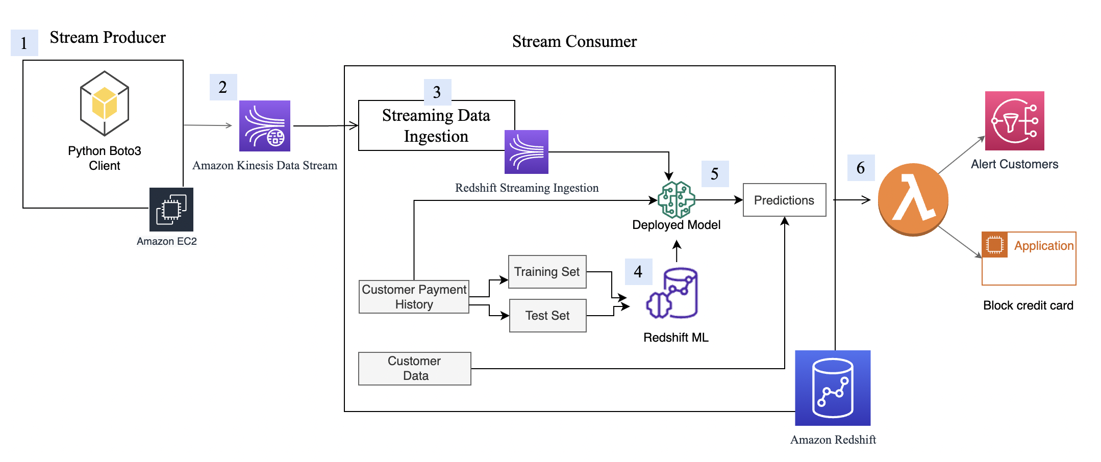
The step-by-step process is as follows:
This walkthrough uses credit card transaction streaming data. The credit card transaction data is fictitious and is based on a simulator. The customer dataset is also fictitious and is generated with some random data functions.
Amazon Kinesis Data Streams is a massively scalable and durable real-time data streaming service. It can continuously capture gigabytes of data per second from hundreds of thousands of sources, such as website clickstreams, database event streams, financial transactions, social media feeds, IT logs, and location-tracking events. The data collected is available in milliseconds to enable real-time analytics use cases such as real-time dashboards, real-time anomaly detection, dynamic pricing, and more. We use Kinesis Data Streams because it’s a serverless solution that can scale based on usage.
First, you need to create a Kinesis data stream to receive the streaming data:
cust-payment-txn-stream.

For a streaming application to write to Kinesis Data Streams, the application needs to have access to Kinesis. You can use the following policy statement to grant the simulator process that you set up in next section access to the data stream. Use the ARN of the data stream that you saved in the previous step.
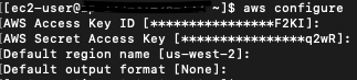
Before we can consume streaming data in Amazon Redshift, we need a streaming data source that writes data to the Kinesis data stream. This post uses a custom-built data generator and the AWS SDK for Python (Boto3) to publish the data to the data stream. For setup instructions, refer to Producer Simulator. This simulator process publishes streaming data to the data stream created in the previous step (cust-payment-txn-stream).
This section talks about configuring the stream consumer (the Amazon Redshift streaming ingestion view).
Amazon Redshift Streaming Ingestion provides low-latency, high-speed ingestion of streaming data from Kinesis Data Streams into an Amazon Redshift materialized view. You can configure your Amazon Redshift cluster to enable streaming ingestion and create a materialized view with auto refresh, using SQL statements, as described in Creating materialized views in Amazon Redshift. The automatic materialized view refresh process will ingest streaming data at hundreds of megabytes of data per second from Kinesis Data Streams into Amazon Redshift. This results in fast access to external data that is quickly refreshed.
After creating the materialized view, you can access your data from the data stream using SQL and simplify your data pipelines by creating materialized views directly on top of the stream.
Complete the following steps to configure an Amazon Redshift streaming materialized view:
KinesisStreamPolicy. For the streaming policy definition, see Getting started with streaming ingestion.redshift-streaming-role and attach the policy KinesisStreamPolicy.Now you can create a materialized view to consume the stream data. You can use the SUPER data type to store the payload as is, in JSON format, or use Amazon Redshift JSON functions to parse the JSON data into individual columns. For this post, we use the second method because the schema is well defined.
cust_payment_tx_stream. By specifying AUTO REFRESH YES in the following code, you can enable automatic refresh of the streaming ingestion view, which saves time by avoiding building data pipelines:Note that json_extract_path_text has a length limitation of 64 KB. Also from_varbye filters records larger than 65KB.
The Amazon Redshift streaming materialized view is auto refreshed by Amazon Redshift for you. This way, you don’t need worry about data staleness. With materialized view auto refresh, data is automatically loaded into Amazon Redshift as it becomes available in the stream. If you choose to manually perform this operation, use the following command:
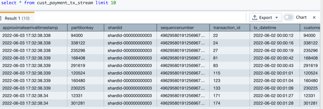

Now you have finished setting up the Amazon Redshift streaming ingestion view, which is continuously updated with incoming credit card transaction data. In my setup, I see that around 67,000 records have been pulled into the streaming view at the time when I ran my select count query. This number could be different for you.
With Redshift ML, you can bring a pre-trained ML model or build one natively. For more information, refer to Using machine learning in Amazon Redshift.
In this post, we train and build an ML model using a historical dataset. The data contains a tx_fraud field that flags a historical transaction as fraudulent or not. We build a supervised ML model using Redshift Auto ML, which learns from this dataset and predicts incoming transactions when those are run through the prediction functions.
In the following sections, we show how to set up the historical dataset and customer data.
The historical table has more fields than what the streaming data source has. These fields contain the customer’s most recent spend and terminal risk score, like number of fraudulent transactions computed by transforming streaming data. There are also categorical variables like weekend transactions or nighttime transactions.
To load the historical data, run the commands using the Amazon Redshift query editor.
Create the transaction history table with the following code. The DDL can also be found on GitHub.
Let’s check how many transactions are loaded:
Check the monthly fraud and non-fraud transactions trend:
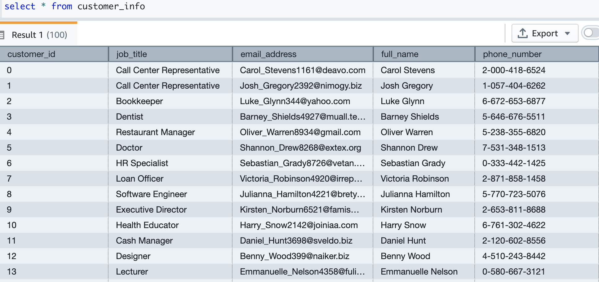
Now we create the customer table and load data, which contains the email and phone number of the customer. The following code creates the table, loads the data, and samples the table. The table DDL is available on GitHub.
Our test data has about 5,000 customers. The following screenshot shows sample customer data.
Our historical card transaction table has 6 months of data, which we now use to train and test the ML model.
The model takes the following fields as input:
We get tx_fraud as output.
We split this data into training and test datasets. Transactions from 2022-04-01 to 2022-07-31 are for the training set. Transactions from 2022-08-01 to 2022-09-30 are used for the test set.
Let’s create the ML model using the familiar SQL CREATE MODEL statement. We use a basic form of the Redshift ML command. The following method uses Amazon SageMaker Autopilot, which performs data preparation, feature engineering, model selection, and training automatically for you. Provide the name of your S3 bucket containing the code.
I call the ML model as Cust_cc_txn_fd, and the prediction function as fn_customer_cc_fd. The FROM clause shows the input columns from the historical table public.cust_payment_tx_history. The target parameter is set to tx_fraud, which is the target variable that we’re trying to predict. IAM_Role is set to default because the cluster is configured with this role; if not, you have to provide your Amazon Redshift cluster IAM role ARN. I set the max_runtime to 3,600 seconds, which is the time we give to SageMaker to complete the process. Redshift ML deploys the best model that is identified in this time frame.
Depending on the complexity of the model and the amount of data, it can take some time for the model to be available. If you find your model selection is not completing, increase the value for max_runtime. You can set a max value of 9999.
The CREATE MODEL command is run asynchronously, which means it runs in the background. You can use the SHOW MODEL command to see the status of the model. When the status shows as Ready, it means the model is trained and deployed.
The following screenshots show our output.
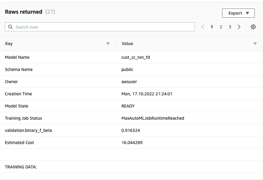
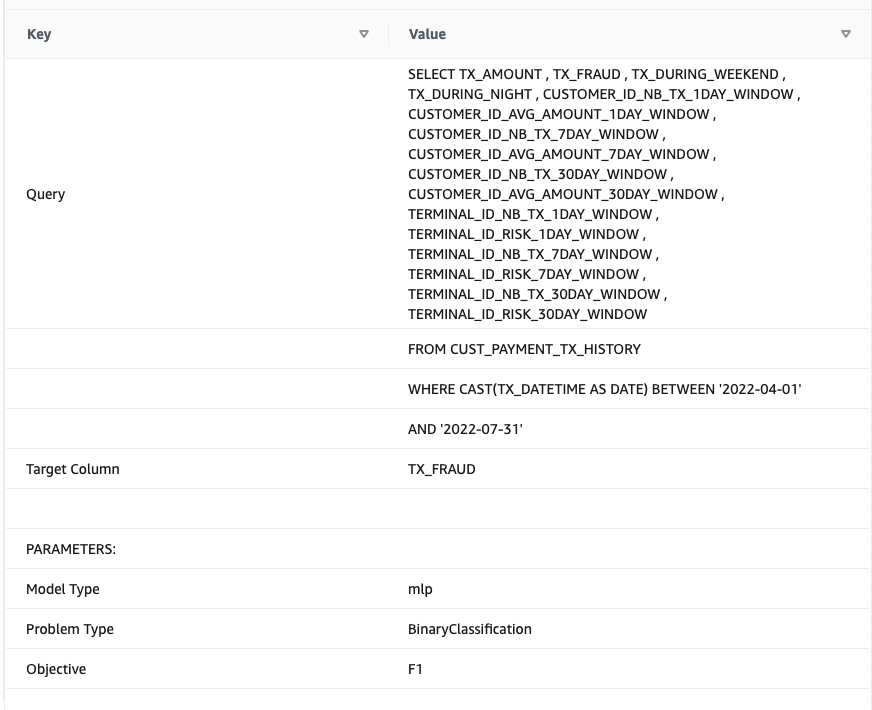
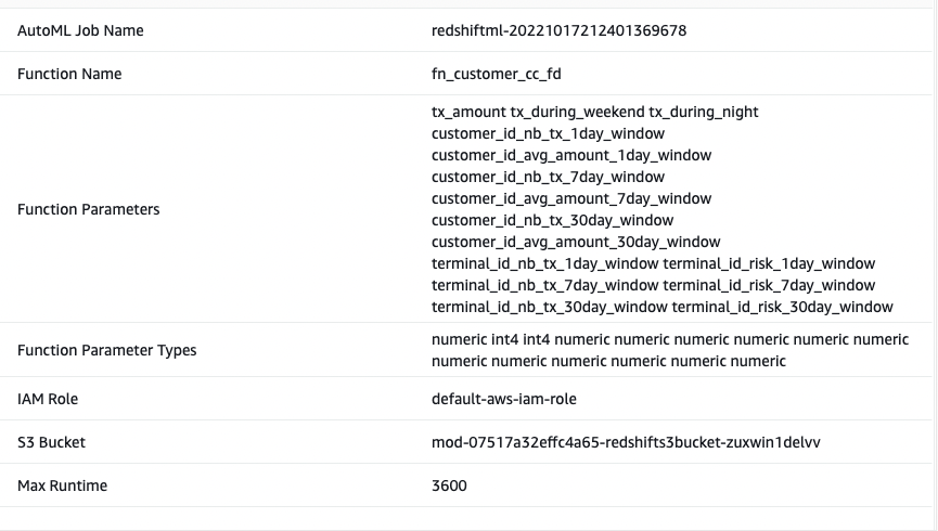
From the output, I see that the model has been correctly recognized as BinaryClassification, and F1 has been selected as the objective. The F1 score is a metric that considers both precision and recall. It returns a value between 1 (perfect precision and recall) and 0 (lowest possible score). In my case, it’s 0.91. The higher the value, the better the model performance.
Let’s test this model with the test dataset. Run the following command, which retrieves sample predictions:
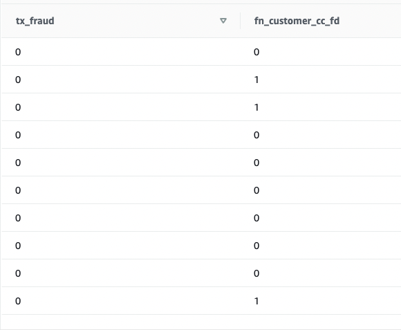
We see that some values are matching and some are not. Let’s compare predictions to the ground truth:
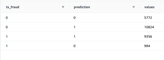
We validated that the model is working and the F1 score is good. Let’s move on to generating predictions on streaming data.
Because the Redshift ML model is ready to use, we can use it to run the predictions against streaming data ingestion. The historical dataset has more fields than what we have in the streaming data source, but they’re just recency and frequency metrics around the customer and terminal risk for a fraudulent transaction.
We can apply the transformations on top of the streaming data very easily by embedding the SQL inside the views. Create the first view, which aggregates streaming data at the customer level. Then create the second view, which aggregates streaming data at terminal level, and the third view, which combines incoming transactional data with customer and terminal aggregated data and calls the prediction function all in one place. The code for the third view is as follows:
Run a SELECT statement on the view:
As you run the SELECT statement repeatedly, the latest credit card transactions go through transformations and ML predictions in near-real time.
This demonstrates the power of Amazon Redshift—with easy-to-use SQL commands, you can transform streaming data by applying complex window functions and apply an ML model to predict fraudulent transactions all in one step, without building complex data pipelines or building and managing additional infrastructure.
Because the data streams in and ML predictions are made in near-real time, you can build business processes for alerting your customer using Amazon Simple Notification Service (Amazon SNS), or you can lock the customer’s credit card account in an operational system.
This post doesn’t go into the details of these operations, but if you’re interested in learning more about building event-driven solutions using Amazon Redshift, refer to the following GitHub repository.
To avoid incurring future charges, delete the resources that were created as part of this post.
In this post, we demonstrated how to set up a Kinesis data stream, configure a producer and publish data to streams, and then create an Amazon Redshift Streaming Ingestion view and query the data in Amazon Redshift. After the data was in the Amazon Redshift cluster, we demonstrated how to train an ML model and build a prediction function and apply it against the streaming data to generate predictions near-real time.
If you have any feedback or questions, please leave them in the comments.
 Bhanu Pittampally is an Analytics Specialist Solutions Architect based out of Dallas. He specializes in building analytic solutions. His background is in data warehouses—architecture, development, and administration. He has been in the data and analytics field for over 15 years.
 Praveen Kadipikonda is a Senior Analytics Specialist Solutions Architect at AWS based out of Dallas. He helps customers build efficient, performant, and scalable analytic solutions. He has worked with building databases and data warehouse solutions for over 15 years.
 Ritesh Kumar Sinha is an Analytics Specialist Solutions Architect based out of San Francisco. He has helped customers build scalable data warehousing and big data solutions for over 16 years. He loves to design and build efficient end-to-end solutions on AWS. In his spare time, he loves reading, walking, and doing yoga.
Post Syndicated from Jonatan Selsing original https://aws.amazon.com/blogs/big-data/how-novo-nordisk-built-a-modern-data-architecture-on-aws/
Novo Nordisk is a leading global pharmaceutical company, responsible for producing life-saving medicines that reach more than 34 million patients each day. They do this following their triple bottom line—that they must strive to be environmentally sustainable, socially sustainable, and financially sustainable. The combination of using AWS and data supports all these targets.
Data is pervasive throughout the entire value chain of Novo Nordisk. From foundational research, manufacturing lines, sales and marketing, clinical trials, pharmacovigilance, through patient-facing data-driven applications. Therefore, getting the foundation around how data is stored, safeguarded, and used in a way that provides the most value is one of the central drivers of improved business outcomes.
Together with AWS Professional Services, we’re building a data and analytics solution using a modern data architecture. The collaboration between Novo Nordisk and AWS Professional Services is a strategic and long-term close engagement, where developers from both organizations have worked together closely for years. The data and analytics environments are built around of the core tenets of the data mesh—decentralized domain ownership of data, data as a product, self-service data infrastructure, and federated computational governance. This enables the users of the environment to work with data in the way that drives the best business outcomes. We have combined this with elements from evolutionary architectures that will allow us to adapt different functionalities as AWS continuously develops new services and capabilities.
In this series of posts, you will learn how Novo Nordisk and AWS Professional Services built a data and analytics ecosystem to speed up innovation at petabyte scale:
As a pharmaceutical industry, GxP compliance is a mandate for Novo Nordisk. GxP is a general abbreviation for the “Good x Practice” quality guidelines and regulations defined by regulators such as European Medicines Agency, U.S. Food and Drug Administration, and others. These guidelines are designed to ensure that medicinal products are safe and effective for their intended use. In the context of a data environment, GxP compliance involves implementing integrity controls for data used to in decision making and processes and is used to guide how change management processes are implemented to continuously ensure compliance over time.
Because this data environment supports teams across the whole organization, each individual data owner must retain accountability on their data. Features were designed to provide data owners autonomy and transparency when managing their data, enabling them to take this responsibility. This includes the capability to handle personally identifiable information (PII) data and other sensitive workloads. To provide traceability on the environment, audit capabilities were added, which we describe more in this post.
The full solution is a sprawling landscape of independent services that work together to enable data and analytics with a decentralized data governance model at petabyte scale. Schematically, it can be represented as in the following figure.
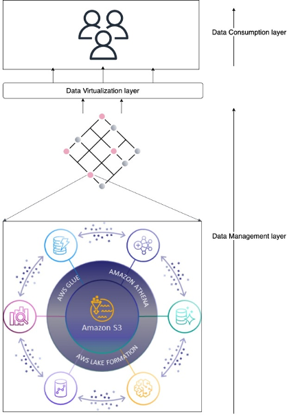
The architecture is split into three independent layers: data management, virtualization, and consumption. The end-user sits in the consumption layer and works with their tool of choice. It’s meant to abstract as much of the AWS-native resources to application primitives. The consumption layer is integrated into the virtualization layer, which abstracts the access to data. The purpose of the virtualization layer is to translate between data consumption and data management solutions. The access to data is managed by what we refer to as data management solutions. We discuss one of our versatile data management solutions later in this post. Each layer in this architecture is independent of each other and instead only relies on well-defined interfaces.
Central to this architecture is that access is encapsulated in an AWS Identity and Access Management (IAM) role session. The data management layer focuses on providing the IAM role with the right permissions and governance, the virtualization layer provides access to the role, and the consumption layer abstracts the use of the roles in the tools of choice.
Each of the three layers in the overall architecture has a distinct responsibility, but no singular implementation. Think of them as abstract classes. They can be implemented in concrete classes, and in our case they rely on foundational AWS services and capabilities. Let’s go through each of the three layers.
The data management layer is responsible for providing access to and governance of data. As illustrated in the following diagram, a minimal construct in the data management layer is the combination of an Amazon Simple Storage Service (Amazon S3) bucket and an IAM role that gives access to the S3 bucket. This construct can be expanded to include granular permission with Lake Formation, auditing with AWS CloudTrail, and security response capabilities from AWS Security Hub. The following diagram also shows that a single data management solution has no singular span. It can cross many AWS accounts and be comprised of any number of IAM role combinations.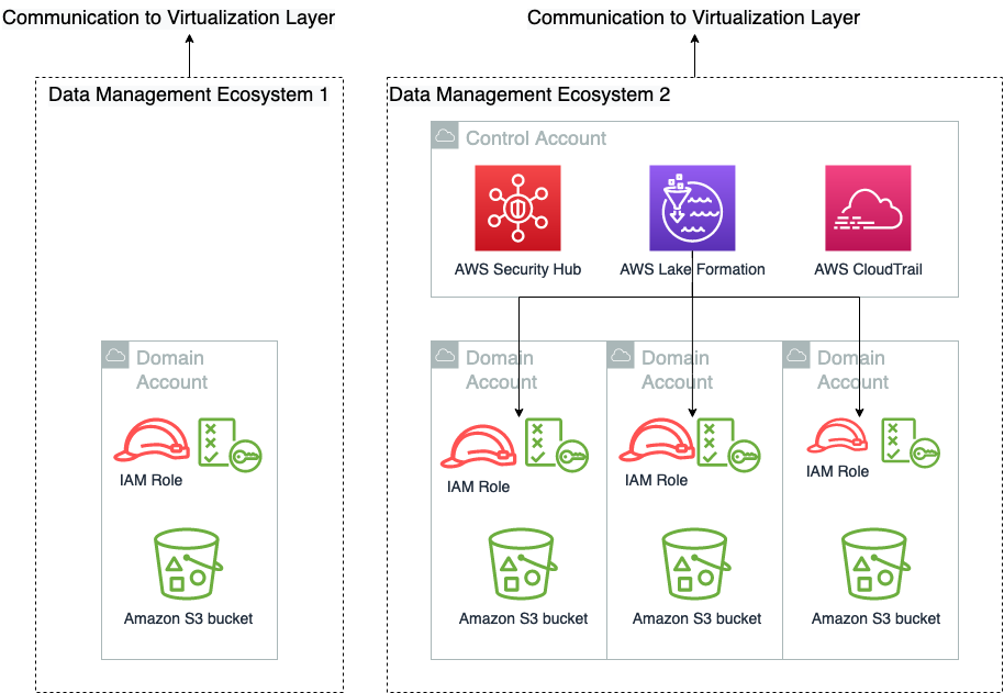
We have purposely not illustrated the trust policy of these roles in this figure, because those are a collaborative responsibility between the virtualization layer and the data management layer. We go into detail of how that works in the next post in this series. Data engineering professionals often interface directly with the data management layer, where they curate and prepare data for consumption.
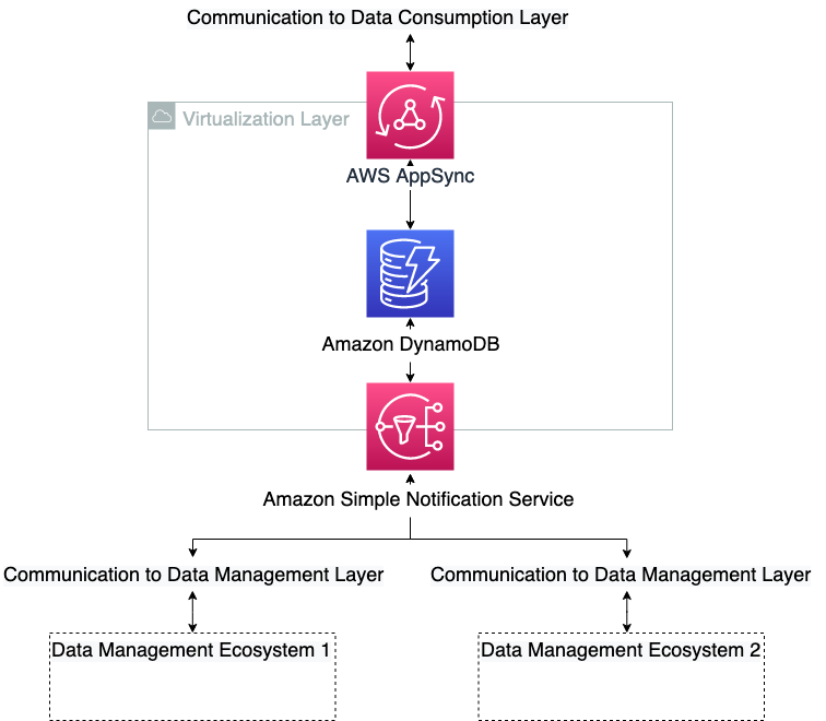
The purpose of the virtualization layer is to keep track of who can do what. It doesn’t have any capabilities in itself, but translates the requirements from the data management ecosystems to the consumption layers and vice versa. It enables end-users on the consumption layer to access and manipulate data on one or more data management ecosystems, according to their permissions. This layer abstracts from end-users the technical details on data access, such as permission model, role assumptions, and storage location. It owns the interfaces to the other layers and enforces the logic of the abstraction. In the context of hexagonal architectures (see Developing evolutionary architecture with AWS Lambda), the interface layer plays the role of the domain logic, ports, and adapters. The other two layers are actors. The data management layer communicates the state of the layer to the virtualization layer and conversely receives information about the service landscape to trust. The virtualization layer architecture is shown in the following diagram.
The consumption layer is where the end-users of the data products are sitting. This can be data scientists, business intelligence analysts, or any third party that generates value from consuming the data. It’s important for this type of architecture that the consumption layer has a hook-based sign-in flow, where the authorization into the application can be modified at sign-in time. This is to translate the AWS-specific requirement into the target applications. After the session in the client-side application has successfully been started, it’s up to the application itself to instrument for data layer abstraction, because this will be application specific. And this is an additional important decoupling, where some responsibility is pushed to the decentralized units. Many modern software as a service (SaaS) applications support these built-in mechanisms, such as Databricks or Domino Data Lab, whereas more traditional client-side applications like RStudio Server have more limited native support for this. In the case where native support is missing, a translation down to the OS user session can be done to enable the abstraction. The consumption layer is shown schematically in the following diagram.
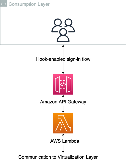
When using the consumption layer as intended, the users don’t know that the virtualization layer exists. The following diagram illustrates the data access patterns.
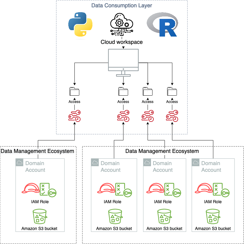
One of the main advantages of adopting the hexagonal architecture pattern, and delegating both the consuming layer and the data management layer to primary and secondary actors, means that they can be changed or replaced as new functionalities are released that require new solutions. This gives a hub-and-spoke type pattern, where many different types of producer/consumer type systems can be connected and work simultaneously in union. An example of this is that the current solution running in Novo Nordisk supports multiple, simultaneous data management solutions and are exposed in a homogenous way in the consuming layer. This includes both a data lake, the data mesh solution presented in this post, and several independent data management solutions. And these are exposed to multiple types of consuming applications, from custom managed, self-hosted applications, to SaaS offerings.
To scale the usage of the data and increase the freedom, Novo Nordisk, jointly with AWS Professional Services, built a data management and governance environment, named Novo Nordisk Enterprise DataHub (NNEDH). NNEDH implements a decentralized distributed data architecture, and data management capabilities such as an enterprise business data catalog and data sharing workflow. NNEDH is an example of a data management ecosystem in the conceptual framework introduced earlier.
Novo Nordisk’s centralized data lake consists of 2.3 PB of data from more than 30 business data domains worldwide serving over 2000+ internal users throughout the value chain. It has been running successfully for several years. It is one of the data management ecosystems currently supported.
Within the centralized data architecture, data from each data domain is copied, stored, and processed in one central location: a central data lake hosted in one data storage. This pattern has challenges at scale because it retains the data ownership with the central team. At scale, this model slows down the journey toward a data-driven organization, because ownership of the data isn’t sufficiently anchored with the professionals closest to the domain.
The monolithic data lake architecture is shown in the following diagram.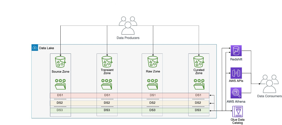
Within the decentralized distributed data architecture, the data from each domain is kept within the domain on its own data storage and compute account. In this case, the data is kept close to domain experts, because they’re the ones who know their own data best and are ultimately the owner of any data products built around their data. They often work closely with business analysts to build the data product and therefore know what good data means to consumers of their data products. In this case, the data responsibility is also decentralized, where each domain has its own data owner, putting the accountability onto the true owners of the data. Nevertheless, this model might not work at small scale, for example an organization with only one business unit and tens of users, because it would introduce more overhead on the IT team to manage the organization data. It better suits large organizations, or small and medium ones that would like to grow and scale.
The Novo Nordisk data mesh architecture is shown in the following diagram.
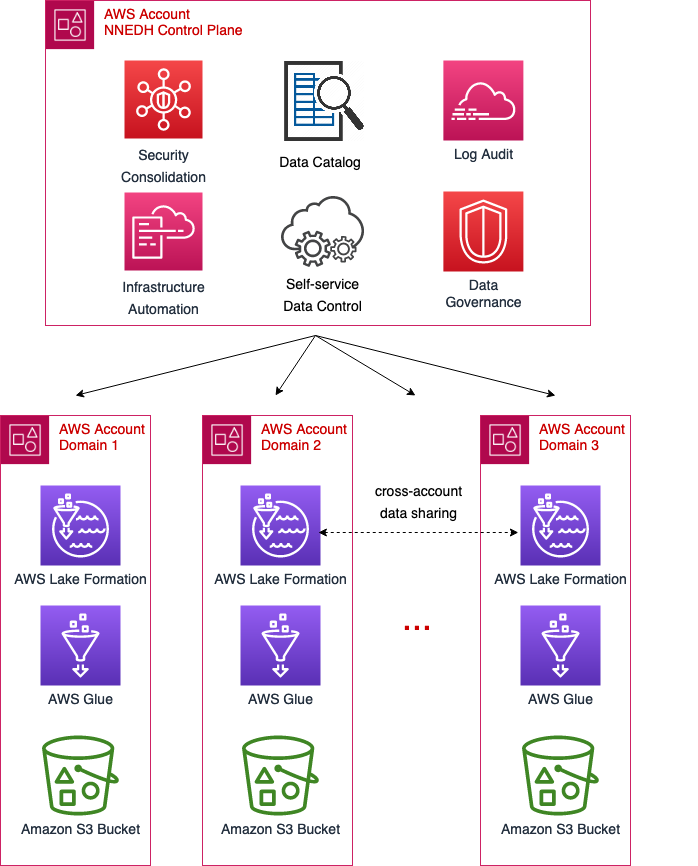
To enable the scalability of data domains across the organization, it’s mandatory to have a standard permission model and data access pattern. This standard must not be too restrictive in such a way that it may be a blocker for specific use cases, but it should be standardized in such a way to use the same interface between the data management and virtualization layers.
The data domains on NNEDH are implemented by a construct called an environment. An environment is composed of at least one AWS account and one AWS Region. It’s a workplace where data domain teams can work and collaborate to build data products. It links the NNEDH control plane to the AWS accounts where the data and compute of the domain reside. The data access permissions are also defined at the environment level, managed by the owner of the data domain. The environments have three main components: a data management and governance layer, data assets, and optional blueprints for data processing.
For data management and governance, the data domains rely on Lake Formation, AWS Glue, and CloudTrail. The deployment method and setup of these components is standardized across data domains. This way, the NNEDH control plane can provide connectivity and management to data domains in a standardized way.
The data assets of each domain residing in an environment are organized in a dataset, which is a collection of related data used for building a data product. It includes technical metadata such as data format, size, and creation time, and business metadata such as the producer, data classification, and business definition. A data product can use one or several datasets. It is implemented through managed S3 buckets and the AWS Glue Data Catalog.
Data processing can be implemented in different ways. NNEDH provides blueprints for data pipelines with predefined connectivity to data assets to speed up the delivery of data products. Data domain users have the freedom to use any other compute capability on their domain, for example using AWS services not predefined on the blueprints or accessing the datasets from other analytics tools implemented in the consumption layer, as mentioned earlier in this post.
On NNEDH, the permission levels on data domains are managed through predefined personas, for example data owner, data stewards, developers, and readers. Each persona is associated with an IAM role that has a predefined permission level. These permissions are based on the typical needs of users on these roles. Nevertheless, to give more flexibility to data domains, these permissions can be customized and extended as needed.
The permissions associated with each persona are related only to actions allowed on the AWS account of the data domain. For the accountability on data assets, the data access to the assets is managed by specific resource policies instead of IAM roles. Only the owner of each dataset, or data stewards delegated by the owner, can grant or revoke data access.
On the dataset level, a required persona is the data owner. Typically, they work closely with one or many data stewards as data products managers. The data steward is the data subject matter expert of the data product domain, responsible for interpreting collected data and metadata to derive deep business insights and build the product. The data steward bridges between business users and technical teams on each data domain.
To enable freedom and make the organization data assets discoverable, a web-based portal data catalog is implemented. It indexes in a single repository metadata from datasets built on data domains, breaking data silos across the organization. The data catalog enables data search and discovery across different domains, as well as automation and governance on data sharing.
The business data catalog implements data governance processes within the organization. It ensures the data ownership—someone in the organization is responsible for the data origin, definition, business attributes, relationships, and dependencies.
The central construct of a business data catalog is a dataset. It’s the search unit within the business catalog, having both technical and business metadata. To collect technical metadata from structured data, it relies on AWS Glue crawlers to recognize and extract data structures from the most popular data formats, including CSV, JSON, Avro, and Apache Parquet. It provides information such as data type, creation date, and format. The metadata can be enriched by business users by adding a description of the business context, tags, and data classification.
The dataset definition and related metadata are stored in an Amazon Aurora Serverless database and Amazon OpenSearch Service, enabling you to run textual queries on the data catalog.
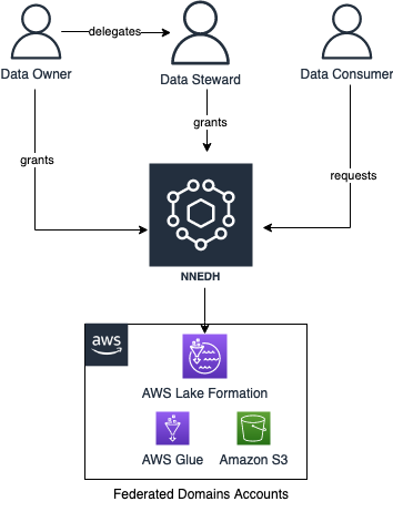
NNEDH implements a data sharing workflow, enabling peer-to-peer data sharing across AWS accounts using Lake Formation. The workflow is as follows:
The data sharing workflow is shown schematically in the following figure.
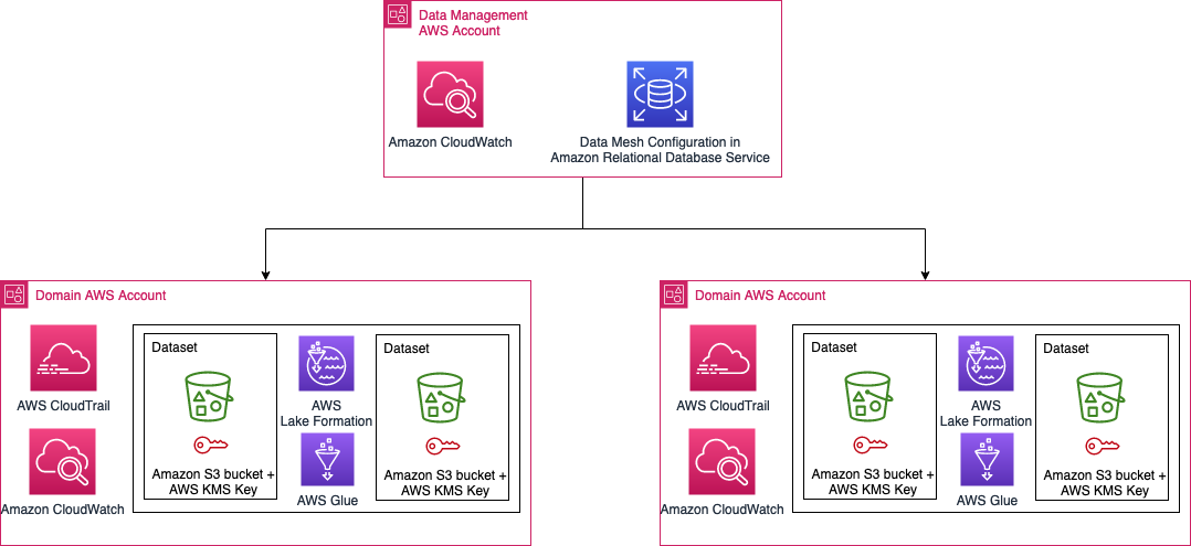
The data in the Novo Nordisk data mesh lies in AWS accounts owned by Novo Nordisk business accounts. The configuration and the states of the data mesh are stored in Amazon Relational Database Service (Amazon RDS). The Novo Nordisk security architecture is shown in the following figure.
Access and edits to the data in NNEDH needs to be logged for audit purposes. We need to be able to tell who modified data, when the modification happened, and what modifications were applied. In addition, we need to be able to answer why the modification was allowed by that person at that time.
To meet these requirements, we use the following components:
In addition to those logging mechanisms, the S3 buckets are created using the following properties:
Access to the data in NNEDH is controlled at the group level instead of individual users. The group corresponds to the group defined in the Novo Nordisk directory group. To keep track of the person who modified the data in the data lakes, we use the source identity mechanism explained in the post How to relate IAM role activity to corporate identity.
In this post, we showed how Novo Nordisk built a modern data architecture to speed up the delivery of data-driven use cases. It includes a distributed data architecture, to scale the usage to petabyte scale for over 2,000 internal users throughout the value chain, as well as a distributed security and audit architecture handling data accountability and traceability on the environment to meet their compliance requirements.
The next post in this series describes the implementation of distributed data governance and control at scale of Novo Nordisk’s modern data architecture.
 Jonatan Selsing is former research scientist with a PhD in astrophysics that has turned to the cloud. He is currently the Lead Cloud Engineer at Novo Nordisk, where he enables data and analytics workloads at scale. With an emphasis on reducing the total cost of ownership of cloud-based workloads, while giving full benefit of the advantages of cloud, he designs, builds, and maintains solutions that enable research for future medicines.
 Hassen Riahi is a Sr. Data Architect at AWS Professional Services. He holds a PhD in Mathematics & Computer Science on large-scale data management. He works with AWS customers on building data-driven solutions.
 Anwar Rizal is a Senior Machine Learning consultant based in Paris. He works with AWS customers to develop data and AI solutions to sustainably grow their business.
 Moses Arthur comes from a mathematics and computational research background and holds a PhD in Computational Intelligence specialized in Graph Mining. He is currently a Cloud Product Engineer at Novo Nordisk building GxP-compliant enterprise data lakes and analytics platforms for Novo Nordisk global factories producing digitalized medical products.
 Alessandro Fior is a Sr. Data Architect at AWS Professional Services. With over 10 years of experience delivering data and analytics solutions, he is passionate about designing and building modern and scalable data platforms that accelerate companies to get value from their data.
 Kumari Ramar is an Agile certified and PMP certified Senior Engagement Manager at AWS Professional Services. She delivers data and AI/ML solutions that speed up cross-system analytics and machine learning models, which enable enterprises to make data-driven decisions and drive new innovations.
Post Syndicated from Dorothy Li original https://aws.amazon.com/blogs/big-data/convoy-uses-amazon-quicksight-to-help-shippers-and-carriers-improve-efficiency-and-save-money-with-data-driven-decisions/
Convoy is the leading digital freight network in the United States. We move millions of truckloads around the country through our connected network of carriers, saving money for shippers, increasing earnings for drivers, and eliminating carbon waste for our planet. In 2015, Convoy started a movement toward efficient freight. We build technology to find smarter ways to connect shippers with carriers while solving some of the toughest problems that result in waste in the freight industry.
As a digital freight network, Convoy uses machine learning and automation to efficiently connect shippers and carriers. As our marketplace grows, it creates a flywheel effect that benefits both sides. As more shippers join the network, drivers have better options, fewer empty miles, and fewer wasted hours, allowing them to earn more per day. As more carriers join the network, capacity increases and shippers see lower costs and higher service quality. Convoy is on a mission to transport the world with endless capacity and zero waste.
Our digital freight network collects thousands of disparate data points and intelligently connects the dots to provide transparent visibility into freight operations. By providing transparency and insights into every step of the shipment lifecycle, shippers benefit from lower costs, reduced waste, and higher carrier loyalty. To surface these insights to customers inside our product, we needed a business intelligence (BI) tool that could not only handle our volume of data, but could provide at-a-glance insights through a user-friendly interface, empowering our customers to make data-driven decisions, and taking the guesswork out of resolving unexpected issues.
After reviewing our options and evaluating which would best meet our needs, we turned to Amazon QuickSight.
In this post, we discuss how QuickSight is helping us serve our customers with the insights they need, and why we consider this business decision a win for Convoy.
Our vast network of small carriers and owner-operators, totaling more than 400,000 trucks nationwide, provides meaningful data points through the Convoy app. We require carriers to use our app when hauling loads—this is how we provide GPS tracking on 95% of live loads and 100% of drop loads. It’s also how we collect robust data around dwell times, detention costs, and more. To date, we’ve captured more than 2.7 million facility reviews in the Convoy app.
We chose QuickSight because we needed ease in development. We wanted to be able to quickly build dashboards and get them in the hands of our customers. Because this is an externally facing tool, we had data privacy and governance requirements to consider as well. Especially important was that we needed granularity in row-level security. QuickSight provided what we needed out of the box, whereas the other BI platforms we considered did not. Additionally, QuickSight’s pricing would allow us to scale the platform as our user base continues to grow.
The challenges facing our customers are as varied as the landscapes our carriers travel through every day. From managing delays due to weather, traffic, and unpredictable load times on the carrier’s end, to lacking freight visibility and root causes of operational issues and inaccuracies in manual reporting on the shipper’s end, there is no shortage of opportunities to improve the status quo.
The following screenshot shows performance metrics, like dwell time and incidentals per shipment, plus breakouts that show incidental types and categories for each facility.

Where we strive to meet the needs of both shippers and carriers, we’re in a unique position to connect the dots to identify gaps on one end that have corresponding inputs on the other. The challenges shippers face are often driven by pricing, complexity, and reliability of transporting goods. For carriers, their challenges are more centered on earning predictable and consistent income with the least amount of time and effort invested in finding loads, building schedules, and adjusting to delays. Our customers have sophisticated internal analytics programs, but highly granular data or synthesized data from their vendors is rare. Finding ways to develop metrics and benchmarks for specific business entities (lanes, regions, facilities, and so on) meant we would need to learn and update our products quickly. QuickSight allows us to do that.
With so many data points and opportunities to turn them into key insights, the dashboards and visualizations QuickSight provides makes spotting trends and taking proactive measures to get ahead of minor issues before they become major problems easier than ever.
When reviewing our BI options, the following factors were front and center in our decision to go with QuickSight:
When we first piloted our external insights product, we built a prototype with our previously used BI tool. Building future iterations with this same tool wasn’t feasible because it lacked functionality in several key areas. We needed to be able to join data from multiple sources, drill down into layers of data, and customize data based on the user accessing the information. In addition, because we were self-hosting, the overhead of scaling our footprint was going to be high. We did consider other solutions, but QuickSight was best able to offer all the features we needed, at the best price.
With QuickSight, we were able to build an external-facing product for our shipper customers, helping them gain visibility into the health of their supply chain, which could then provide insights to make things run more efficiently.
The following screenshot shows incidentals, broken out by spend, type or category, and more.
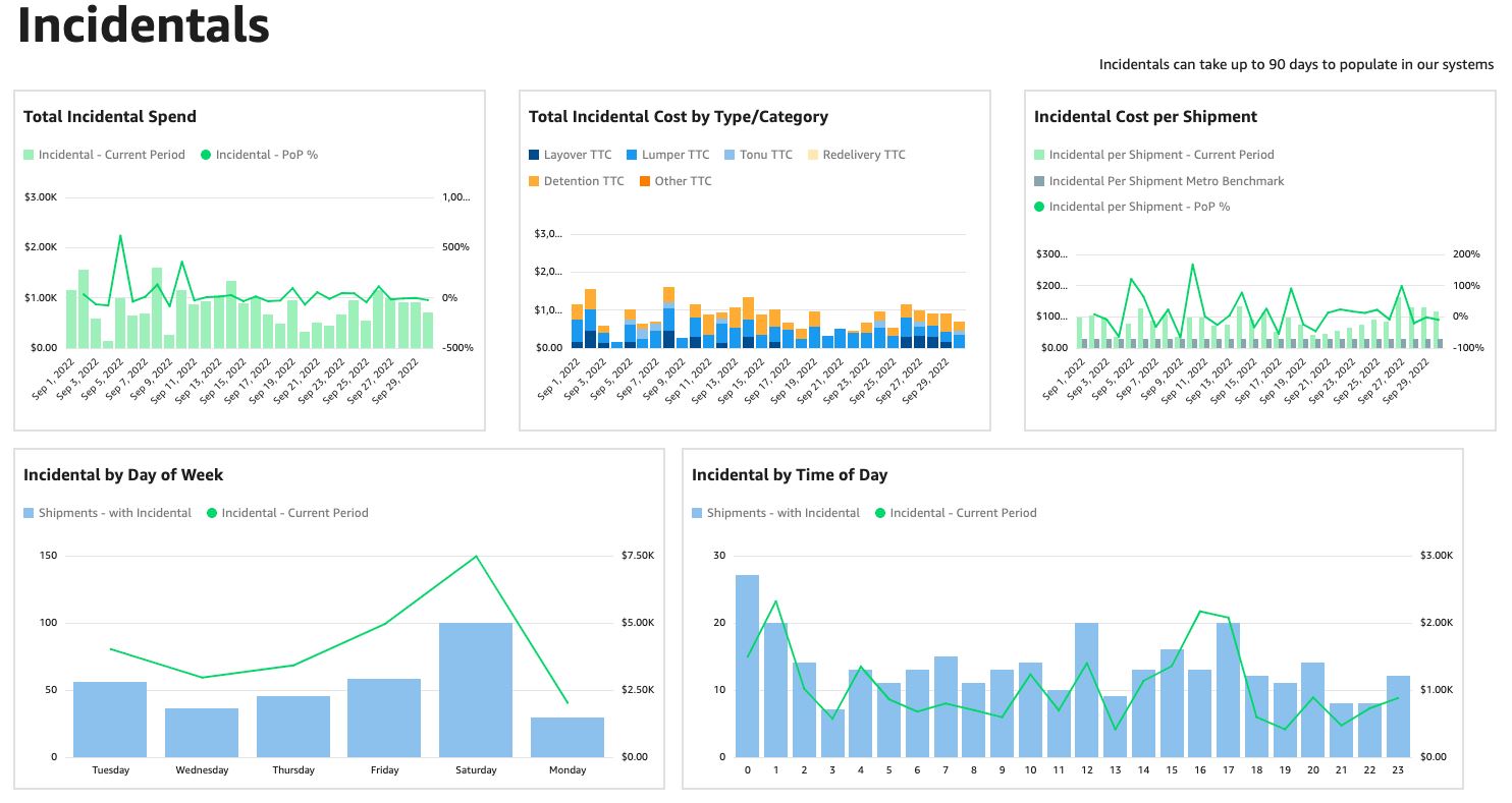
With a visualization of how incidental costs break down, for example, they can see the cost of having a truck unloaded at a facility, the cost of canceling loads on a driver, the cost of having travers waiting at a facility, and more. With that visibility, our shipper customers can now begin to address systemic issues that can save them money, such as improving scheduling to reduce driver wait times.
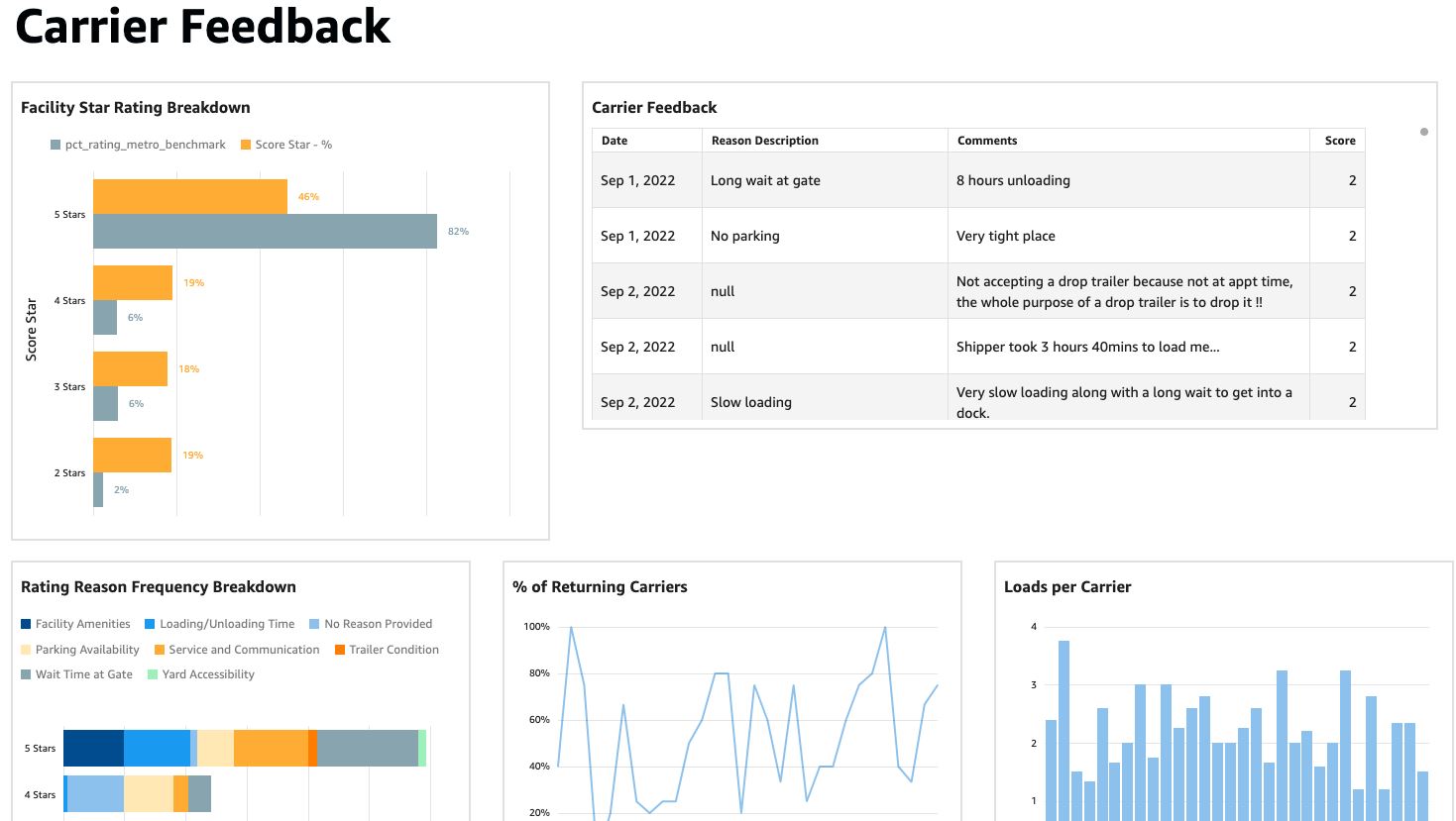
The following screenshot shows a visualization on carrier feedback, which shippers could use to make improvements that provide a faster, smoother experience.
They say that imitation is the purest form of flattery. Although that phrase is often used in the context of competitors who develop products and services that are suspiciously similar to an existing product or service, it can also apply to when good ideas are duplicated within an organization. That’s the case for us, in that our QuickSight adoption has drawn the attention and curiosity of partnering teams, who have reached out to us to understand our implementation specifics and the successes we’ve seen as a result.
We’re very happy with our QuickSight Embedded experience and look forward to continuing to iterate and expand its use for additional customer profiles and use cases.
To learn more about how you can embed customized data visuals, interactive dashboards, and natural language querying into any application, visit Amazon QuickSight Embedded.
 Dorothy Li is Convoy’s CTO, overseeing Convoy’s Product and Engineering group and technology strategy, shaping and scaling the company’s innovation and industry-defining technology platforms. Prior to Convoy, Dorothy held leadership roles at Amazon, most recently as Vice President of BI and Analytics at AWS. During her more than 20 years at Amazon, Dorothy helped build out Amazon’s ecommerce platform and also led and collaborated on products that had visibly impacted customers around the world – from the initial launch of Amazon Prime, to Kindle, and at AWS where she focused on data analytics and BI. Dorothy received her Bachelor of Science at Brigham Young University and studies at Shanghai International Studies University.
Post Syndicated from Jakub Oleksy original https://github.blog/2023-01-04-github-availability-report-december-2022/
In December, we did not experience any incidents that resulted in degraded performance across GitHub services. This report sheds light into an incident that impacted GitHub Packages and GitHub Pages in November.
November 25 16:34 UTC (lasting 1 hour and 56 minutes)
On November 25, 2022 at 14:39 UTC, our alerting systems detected an incident that impacted customers using GitHub Packages and GitHub Pages. The GitHub Packages team initially statused GitHub Packages to yellow, and after assessing impact, it statused to red at 15:06 UTC.
During this incident, customers experienced unavailability of packages for container, npm, and NuGet registries. We were able to serve requests for RubyGems and Maven registries. GitHub Packages’ unavailability also impacted GitHub Pages, as they were not able to pull packages, which resulted in CI build failures. Repository landing pages also saw timeouts while fetching packages information.
GitHub Packages uses a third-party database to store data for the service and the provider was experiencing an outage, which impacted GitHub Packages performance. The first responder connected with the provider’s support team to learn more about the region specific outage. The provider then mitigated the issue before the first responder could do the failover to another region. With the mitigation in place, GitHub Packages started to recover along with GitHub Pages and the repository landing pages.
As follow up action items, the team is exploring options to make GitHub Pages and repository landing pages more resilient to GitHub Packages outages. We are also investigating options where failovers can be performed quickly and automatically in case of regional outages.
Please follow our status page for real-time updates on status changes. To learn more about what we’re working on, check out the GitHub Engineering Blog.
Post Syndicated from Talks at Google original https://www.youtube.com/watch?v=2tNvLtFpq-U
Post Syndicated from Rostislav Markov original https://aws.amazon.com/blogs/architecture/genomics-workflows-part-4-processing-archival-data/
Genomics workflows analyze data at petabyte scale. After processing is complete, data is often archived in cold storage classes. In some cases, like studies on the association of DNA variants against larger datasets, archived data is needed for further processing. This means manually initiating the restoration of each archived object and monitoring the progress. Scientists require a reliable process for on-demand archival data restoration so their workflows do not fail.
In Part 4 of this series, we look into genomics workloads processing data that is archived with Amazon Simple Storage Service (Amazon S3). We design a reliable data restoration process that informs the workflow when data is available so it can proceed. We build on top of the design pattern laid out in Parts 1-3 of this series. We use event-driven and serverless principles to provide the most cost-effective solution.
Our use case focuses on data in Amazon Simple Storage Service Glacier (Amazon S3 Glacier) storage classes. The S3 Glacier Instant Retrieval storage class provides the lowest-cost storage for long-lived data that is rarely accessed but requires retrieval in milliseconds.
The S3 Glacier Flexible Retrieval and S3 Glacier Deep Archive provide further cost savings, with retrieval times ranging from minutes to hours. We focus on the latter in order to provide the most cost-effective solution.
You must first restore the objects before accessing them. Our genomics workflow will pause until the data restore completes. The requirements for this workflow are:
Genomics workflows take multiple input parameters to prepare the initiation, such as launch ID, data path, workflow endpoint, and workflow steps. We store this data, including workflow configurations, in an S3 bucket. An AWS Fargate task reads from the S3 bucket and prepares the workflow. It detects if the input parameters include S3 Glacier URLs.
We use Amazon Simple Queue Service (Amazon SQS) to decouple S3 Glacier index creation from object restore actions (Figure 1). This increases the reliability of our process.

Figure 1. Solution architecture for S3 Glacier object restore
An AWS Lambda function creates the index of all objects in the specified S3 bucket URLs and submits them as an SQS message.
Another Lambda function polls the SQS queue and submits the request(s) to restore the S3 Glacier objects to S3 Standard storage class.
The function writes the job ID of each S3 Glacier restore request to Amazon DynamoDB. After the restore is complete, Lambda sets the status of the workflow to READY. Only then can any computing jobs start, such as with AWS Batch.
We consider the use case of Snakemake with Tibanna, which we detailed in Part 2 of this series. This allows us to dive deeper on launch details.
Snakemake is an open-source utility for whole-genome-sequence mapping in directed acyclic graph format. Snakemake uses Snakefiles to declare workflow steps and commands. Tibanna is an open-source, AWS-native software that runs bioinformatics data pipelines. It supports Snakefile syntax, plus other workflow languages, including Common Workflow Language and Workflow Description Language (WDL).
We recommend using Amazon Genomics CLI if Tibanna is not needed for your use case, or Amazon Omics if your workflow definitions are compliant with the supported WDL and Nextflow specifications.
The Snakemake Fargate launch container detects if the S3 objects under the requested S3 bucket URLs are stored in S3 Glacier. The Fargate launch container generates and puts a JSON binary base call (BCL) configuration file into an S3 bucket and exits successfully. This file includes the launch ID of the workflow, corresponding with the DynamoDB item key, plus the S3 URLs to restore.
Once the JSON BCL configuration file lands in this S3 bucket, the S3 Event Notification PutObject event invokes a Lambda function. This function parses the configuration file and recursively queries for all S3 object URLs to restore.
The main Lambda function then submits messages to the SQS queue that contains the full list of S3 URLs that need to be restored. SQS messages also include the launch ID of the workflow. This is to ensure we can bind specific restoration jobs to specific workflow launches. If all S3 Glacier objects belong to Flexible Retrieval storage class, the Lambda function puts the URLs in a single SQS message, enabling restoration with Bulk Glacier Job Tier. The Lambda function also sets the status of the workflow to WAITING in the corresponding DynamoDB item. The WAITING state is used to notify the end user that the job is waiting on the data-restoration process and will continue once the data restoration is complete.
A secondary Lambda function polls for new messages landing in the SQS queue. This Lambda function submits the restoration request(s)—for example, as a free-of-charge Bulk retrieval—using the RestoreObject API. The function subsequently writes the S3 Glacier Job ID of each request in our DynamoDB table. This allows the main Lambda function to check if all Job IDs associated with a workflow launch ID are complete.
The status of our workflow launch will remain WAITING as long as the Glacier object restore is incomplete. The AWS CloudTrail logs of completed S3 Glacier Job IDs invoke our main Lambda function (via an Amazon EventBridge rule) to update the status of the restoration job in our DynamoDB table. With each invocation, the function checks if all Job IDs associated with a workflow launch ID are complete.
After all objects have been restored, the function updates the workflow launch with status READY. This launches the workflow with the same launch ID prior to the restore.
In this blog post, we demonstrated how life-science research teams can make use of their archival data for genomic studies. We designed an event-driven S3 Glacier restore process, which retrieves data upon request. We discussed how to reliably launch the restore so our workflow doesn’t fail. Also, we determined upfront if an S3 Glacier restore is needed and used the WAITING state to prevent our workflow from failing.
With this solution, life-science research teams can save money using Amazon S3 Glacier without worrying about their day-to-day work or manually administering S3 Glacier object restores.
Post Syndicated from Tom Moore original https://aws.amazon.com/blogs/devops/building-net-7-applications-with-aws-codebuild/
AWS CodeBuild is a fully managed DevOps service for building and testing your applications. As a fully managed service, there is no infrastructure to manage and you pay only for the resources that you use when you are building your applications. CodeBuild provides a default build image that contains the current Long Term Support (LTS) version of the .NET SDK.
Microsoft released the latest version of .NET in November. This release, .NET 7, includes performance improvements and functionality, such as native ahead of time compilation. (Native AoT)..NET 7 is a Standard Term Support release of the .NET SDK. At this point CodeBuild’s default image does not support .NET 7. For customers that want to start using.NET 7 right away in their applications, CodeBuild provides two means of customizing your build environment so that you can take advantage of .NET 7.
The first option for customizing your build environment is to provide CodeBuild with a container image you create and maintain. With this method, customers can define the build environment exactly as they need by including any SDKs, runtimes, and tools in the container image. However, this approach requires customers to maintain the build environment themselves, including patching and updating the tools. This approach will not be covered in this blog post.
A second means of customizing your build environment is by using the install phase of the buildspec file. This method uses the default CodeBuild image, and adds additional functionality at the point that a build starts. This has the advantage that customers do not have the overhead of patching and maintaining the build image.
Complete documentation on the syntax of the buildspec file can be found here:
https://docs.aws.amazon.com/codebuild/latest/userguide/build-spec-ref.html
Your application’s buildspec.yml file contains all of the commands necessary to build your application and prepare it for deployment. For a typical .NET application, the buildspec file will look like this:
You might want to say that you are not covering this in the post.
Note: This build spec file contains only the commands to build the application, commands for packaging and storing build artifacts have been omitted for brevity.
In order to add the .NET 7 SDK to CodeBuild so that we can build your .NET 7 applications, we will leverage the install phase of the buildspec file. The install phase allows you to install any third-party libraries or SDKs prior to beginning your actual build.
The above command downloads the Microsoft install script for .NET and uses that script to download and install the latest version of the .NET SDK, from the Standard Term Support channel. This script will download files and set environment variables within the containerized build environment. You can use this same command to automatically pull the latest Long Term Support version of the .NET SDK by changing the command argument STS to LTS.
Your updated buildspec file will look like this:
Once you check in your buildspec file, you can start a build via the CodeBuild console, and your .NET application will be built using the .NET 7 SDK.
As your build runs you will see output similar to this:
Adding .NET 7 support to AWS CodeBuild is easily accomplished by adding a single line to your application’s buildspec.yml file, stored alongside your application source code. This change allows you to keep up to date with the latest versions of .NET while still taking advantage of the managed runtime provided by the CodeBuild service.
About the author:
Post Syndicated from Christina Luconi original https://blog.rapid7.com/2023/01/04/rapid7-announces-global-days-off-to-support-employees-in-2023/

On January 3rd, it was a little bit quieter than usual here at Rapid7. That’s because our offices were closed for our first of five Global Days Off for 2023.
Global Days Off are designed to encourage teams around the world to unplug and rest, enabling them to bring their best selves back to work. At Rapid7, we care for our employees and believe these days will enable our teams to rest and recharge together, so we can continue to create positive outcomes for customers.
We already offer generous or unlimited paid time off plans, as well as a high level of flexibility in how our people structure their days. However, we all recognize that it can be difficult to step away from our work, especially when that work is so impactful. Global Days Off are aimed at providing relief throughout the year.
Days are strategically placed throughout the year, either extending existing holidays or weekends, or providing much needed relief during stretches of the year without holidays. They provide an opportunity for our people to enjoy a day off without feeling the urge to “check in,” having to miss out on meetings, or sift through an overcrowded inbox upon their return.
We are in the process of creating an updated service schedule for shift teams that directly monitor and support customers, so everyone can enjoy time off without impacting our customers.
We’ve always done our best to balance the well being of our team, while delivering the best outcomes for our customers—especially over the last few years. By continuing to invest and align our people strategy and actions with our business goals, we are well positioned to create impact for our customers, our employees, and our industry.
If you’d like to learn more about the important and impactful work our teams are doing around the globe, check out our careers site.
Post Syndicated from BeardedTinker original https://www.youtube.com/watch?v=KLl0ziG4IYc
Post Syndicated from original https://lwn.net/Articles/919052/
The
6.1.3,
6.0.17, and
5.10.162
stable kernel updates have been released. Each contains a moderate set of
important fixes.
Post Syndicated from original https://lwn.net/Articles/919051/
Security updates have been issued by Fedora (xorg-x11-server-Xwayland), Red Hat (webkit2gtk3), SUSE (rmt-server), and Ubuntu (freeradius).
Post Syndicated from Michael Tremante original https://blog.cloudflare.com/waf-content-scanning/

Let’s assume you manage a job advert site. On a daily basis job-seekers will be uploading their CVs, cover letters and other supplementary documents to your servers. What if someone tried to upload malware instead?
Today we’re making your security team job easier by providing a file content scanning engine integrated with our Web Application Firewall (WAF), so that malicious files being uploaded by end users get blocked before they reach application servers.
Enter WAF Content Scanning.
If you are an enterprise customer, reach out to your account team to get access.
At Cloudflare, we pride ourselves on making our products very easy to use. WAF Content Scanning was built with that goal in mind. The main requirement to use the Cloudflare WAF is that application traffic is proxying via the Cloudflare network. Once that is done, turning on Content Scanning requires a single API call.
Once on, the WAF will automatically detect any content being uploaded, and when found, scan it and provide the results for you to use when writing WAF Custom Rules or reviewing security analytics dashboards.
The entire process runs inline with your HTTP traffic and requires no change to your application.
As of today, we scan files up to 1 MB. You can easily block files that exceed this size or perform other actions such as log the upload.
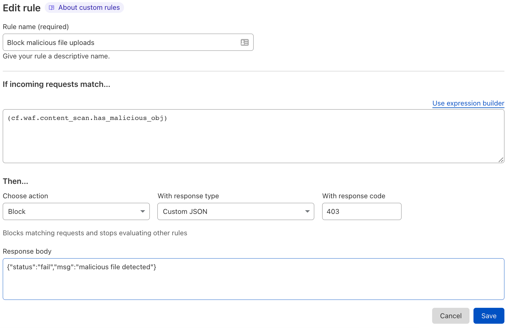
To block a malicious file, you could write a simple WAF Custom Rule like the following:
if: (cf.waf.content_scan.has_malicious_obj)
then: BLOCK
In the dashboard the rule would look like this:

Many other use cases can be achieved by leveraging the metadata exposed by the WAF Content Scanning engine. For example, let’s say you only wanted to allow PDF files to be uploaded on a given endpoint. You would achieve this by deploying the following WAF Custom Rule:
if: any(cf.waf.content_scan.obj_types[*] != "application/pdf") and http.request.uri.path eq "/upload"
then: BLOCK
This rule will, for any content file being uploaded to the /upload endpoint, block the HTTP request if at least one file is not a PDF.
More generally, let’s assume your application does not expect content to be uploaded at all. In this case, you can block any upload attempts with:
if: (cf.waf.content_scan.has_obj)
then: BLOCK
Another very common use case is supporting file upload endpoints that accept JSON content. In this instance files are normally embedded into a JSON payload after being base64-encoded. If your application has such an endpoint, you can provide additional metadata to the scanning engine to recognise the traffic by submitting a custom scan expression. Once submitted, files within JSON payloads will be parsed, decoded, and scanned automatically. In the event you want to issue a block action, you can use a JSON custom response type so that your web application front end can easily parse and display error messages:
The full list of fields exposed by the WAF Content Scanning engine can be found on our developer documentation.
A lot of time designing the system was spent defining what should be scanned. Defining this properly helps us ensure that we are not scanning unnecessary content reducing latency impact and CPU usage, and that there are no bypasses making the system complementary to existing WAF functionality.
The complexity stems from the fact that there is no clear definition of a “file” in HTTP terms. That’s why in this blog post and in the system design, we refer to “content object” instead.
At a high level, although this can loosely be defined as a “file”, not all “content objects” may end up being stored in the file system of an application server! Therefore, we need a definition that applies to HTTP. Additional complexity is given by the fact this is a security product, and attackers will always try to abuse HTTP to obfuscate/hide true intentions. So for example, although a Content-Type header may indicate that the request body is a jpeg image, it may actually be a pdf.
With the above in mind, a “content object” as of today, is any request payload that is detected by heuristics (so no referring to the Content-Type header) to be anything that is not text/html, text/x-shellscript, application/json or text/xml. All other content types are considered a content object.
Detecting via heuristics the content type of an HTTP request body is not enough, as content objects might be found within portions of the HTTP body or encoded following certain rules, such as when using multipart/form-data, which is the most common encoding used when creating standard HTML file input forms.
So when certain payload formats are found, additional parsing applies. As of today the engine will automatically parse and perform content type heuristics on individual components of the payload, when the payload is either encoded using multipart/form-data or multipart/mixed or a JSON string that may have “content objects” embedded in base64 format as defined by the customer
In these cases, we don’t scan the entire payload as a single content object, but we parse it following the relevant standard and apply scanning, if necessary, to the individual portions of the payload. That allows us to support scanning of more than one content object per request, such as an HTML form that has multiple file inputs. We plan to add additional automatic detections in the future on complex payloads moving forward.
In the event we end up finding a malicious match, but we were not able to detect the content type correctly, we will default to reporting a content type of application/octet-stream in the Cloudflare logs/dashboards.
Finally, it is worth noting that we explicitly avoid scanning anything that is plain text (HTML, JSON, XML etc.) as finding attack vectors in these payloads is already covered by the WAF, API Gateway and other web application security solutions already present in Cloudflare’s portfolio.
At Cloudflare, we try to leverage our horizontal architecture to build scalable software. This means the underlying scanner is deployed on every server that handles customer HTTP/S traffic. The diagram below describes the setup:
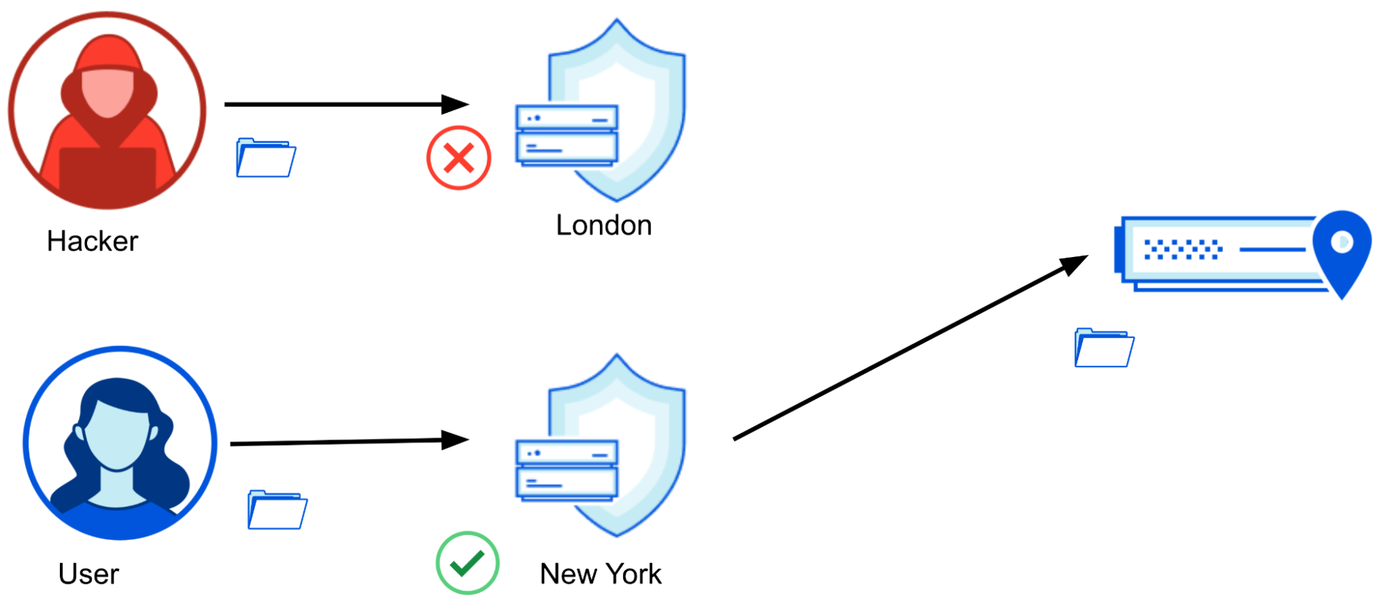
Having each server perform the scanning locally helps ensure latency impact is reduced to a minimum to applicable HTTP requests. The actual scanning engine is the same one used by the Cloudflare Web Gateway, our forward proxy solution that among many other things, helps keep end user devices safe by blocking attempts to download malware.
Consequently, the scanning capabilities provided match those exposed by the Web Gateway AV scanning. The main difference as of today, is the maximum file size currently limited at 1 MB versus 15 MB in Web Gateway. We are working on increasing this to match the Web Gateway in the coming months.
A new approach that we are adopting within our application security portfolio is the separation of detection from mitigation. The WAF Content Scanning features follow this approach, as once turned on, it simply enhances all available data and fields with scan results. The benefits here are twofold.
First, this allows us to provide visibility into your application traffic, without you having to deploy any mitigation. This automatically opens up a great use case: discovery. For large enterprise applications security teams may not be aware of which paths or endpoints might be expecting file uploads from the Internet. Using our WAF Content Scanning feature in conjunction with our new Security Analytics they can now filter on request traffic that has a file content object (a file being uploaded) to observe top N paths and hostnames, exposing such endpoints.

Second, as mentioned in the prior section, exposing the intelligence provided by Cloudflare as fields that can be used in our WAF Custom Rules allows us to provide a very flexible platform. As a plus, you don’t need to learn how to use a new feature, as you are likely already familiar with our WAF Custom Rule builder.
This is not a novel idea, and our Bot Management solution was the first to trial it with great success. Any customer who uses Bot Management today gains access to a bot score field that indicates the likelihood of a request coming from automation or a human. Customers use this field to deploy rules that block bots.
To that point, let’s assume you run a job applications site, and you do not wish for bots and crawlers to automatically submit job applications. You can now block file uploads coming from bots!
if: (cf.bot_management.score lt 10 and cf.waf.content_scan.has_obj)
then: BLOCK
And that’s the power we wish to provide at your fingertips.
Our WAF Content Scanning is a new feature, and we have several improvements planned, including increasing the max content size scanned, exposing the “rewrite” action, so you can send malicious files to a quarantine server, and exposing better analytics that allow you to explore the data more easily without deploying rules. Stay tuned!
Post Syndicated from The History Guy: History Deserves to Be Remembered original https://www.youtube.com/watch?v=GddQUKX3SWU
Post Syndicated from Bruce Schneier original https://www.schneier.com/blog/archives/2023/01/decarbonizing-cryptocurrencies-through-taxation.html
Maintaining bitcoin and other cryptocurrencies causes about 0.3 percent of global CO2 emissions. That may not sound like a lot, but it’s more than the emissions of Switzerland, Croatia, and Norway combined. As many cryptocurrencies crash and the FTX bankruptcy moves into the litigation stage, regulators are likely to scrutinize the cryptocurrency world more than ever before. This presents a perfect opportunity to curb their environmental damage.
The good news is that cryptocurrencies don’t have to be carbon intensive. In fact, some have near-zero emissions. To encourage polluting currencies to reduce their carbon footprint, we need to force buyers to pay for their environmental harms through taxes.
The difference in emissions among cryptocurrencies comes down to how they create new coins. Bitcoin and other high emitters use a system called “proof of work“: to generate coins, participants, or “miners,” have to solve math problems that demand extraordinary computing power. This allows currencies to maintain their decentralized ledger—the blockchain—but requires enormous amounts of energy.
Greener alternatives exist. Most notably, the “proof of stake” system enables participants to maintain their blockchain by depositing cryptocurrency holdings in a pool. When the second-largest cryptocurrency, Ethereum, switched from proof of work to proof of stake earlier this year, its energy consumption dropped by more than 99.9% overnight.
Bitcoin and other cryptocurrencies probably won’t follow suit unless forced to, because proof of work offers massive profits to miners—and they’re the ones with power in the system. Multiple legislative levers could be used to entice them to change.
The most blunt solution is to ban cryptocurrency mining altogether. China did this in 2018, but it only made the problem worse; mining moved to other countries with even less efficient energy generation, and emissions went up. The only way for a mining ban to meaningfully reduce carbon emissions is to enact it across most of the globe. Achieving that level of international consensus is, to say the least, unlikely.
A second solution is to prohibit the buying and selling of proof-of-work currencies. The European Parliament’s Committee on Economic and Monetary Affairs considered making such a proposal, but voted against it in March. This is understandable; as with a mining ban, it would be both viewed as paternalistic and difficult to implement politically.
Employing a tax instead of an outright ban would largely skirt these issues. As with taxes on gasoline, tobacco, plastics, and alcohol, a cryptocurrency tax could reduce real-world harm by making consumers pay for it.
Most ways of taxing cryptocurrencies would be inefficient, because they’re easy to circumvent and hard to enforce. To avoid these pitfalls, the tax should be levied as a fixed percentage of each proof-of-work-cryptocurrency purchase. Cryptocurrency exchanges should collect the tax, just as merchants collect sales taxes from customers before passing the sum on to governments. To make it harder to evade, the tax should apply regardless of how the proof-of-work currency is being exchanged—whether for a fiat currency or another cryptocurrency. Most important, any state that implements the tax should target all purchases by citizens in its jurisdiction, even if they buy through exchanges with no legal presence in the country.
This sort of tax would be transparent and easy to enforce. Because most people buy cryptocurrencies from one of only a few large exchanges—such as Binance, Coinbase, and Kraken—auditing them should be cheap enough that it pays for itself. If an exchange fails to comply, it should be banned.
Even a small tax on proof-of-work currencies would reduce their damage to the planet. Imagine that you’re new to cryptocurrency and want to become a first-time investor. You’re presented with a range of currencies to choose from: bitcoin, ether, litecoin, monero, and others. You notice that all of them except ether add an environmental tax to your purchase price. Which one do you buy?
Countries don’t need to coordinate across borders for a proof-of-work tax on their own citizens to be effective. But early adopters should still consider ways to encourage others to come on board. This has precedent. The European Union is trying to influence global policy with its carbon border adjustments, which are designed to discourage people from buying carbon-intensive products abroad in order to skirt taxes. Similar rules for a proof-of-work tax could persuade other countries to adopt one.
Of course, some people will try to evade the tax, just as people evade every other tax. For example, people might buy tax-free coins on centralized exchanges and then swap them for polluting coins on decentralized exchanges. To some extent, this is inevitable; no tax is perfect. But the effort and technical know-how needed to evade a proof-of-work tax will be a major deterrent.
Even if only a few countries implement this tax—and even if some people evade it—the desirability of bitcoin will fall globally, and the environmental benefit will be significant. A high enough tax could also cause a self-reinforcing cycle that will drive down these cryptocurrencies’ prices. Because the value of many cryptocurrencies rely largely on speculation, they are dependent on future buyers. When speculators are deterred by the tax, the lack of demand will cause the price of bitcoin to fall, which could prompt more current holders to sell—further lowering prices and accelerating the effect. Declining prices will pressure the bitcoin community to abandon proof of work altogether.
Taxing proof-of-work exchanges might hurt them in the short run, but it would not hinder blockchain innovation. Instead, it would redirect innovation toward greener cryptocurrencies. This is no different than how government incentives for electric vehicles encourage carmakers to improve green alternatives to the internal combustion engine. These incentives don’t restrict innovation in automobiles—they promote it.
Taxing environmentally harmful cryptocurrencies can gain support across the political spectrum, from people with varied interests. It would benefit blockchain innovators and cryptocurrency researchers by shifting focus from environmental harm to beneficial uses of the technology. It has the potential to make our planet significantly greener. It would increase government revenues.
Even bitcoin maximalists have reason to embrace the proposal: it would offer the bitcoin community a chance to prove it can survive and grow sustainably.
This essay was written with Christos Porios, and previously appeared in the Atlantic.
Post Syndicated from Isabel Ronaldson original https://www.raspberrypi.org/blog/building-community-global-clubs-partners-code-club-coderdojo/
As part of our mission to enable young people to realise their full potential through the power of computing and digital technologies, we work in partnership with organisations around the globe to grow and sustain the Code Club and CoderDojo networks of coding clubs for young people. These organisations are our global clubs partners, and they undertake activities including training educators and volunteers, providing access to equipment, and running clubs and events for young people at a local or national level.

Given that many people at the Raspberry Pi Foundation are based in the UK and Ireland, and that meeting in person has been restricted during the coronavirus pandemic, our work to connect with the global clubs partners network has largely taken place via video calls these last years. We don’t only connect with partners one to one, we also link them to each other so they can share insights, approaches, and resources. Video calls offer a unique opportunity for bringing together partner organisations located all over the world, but they provide a very different experience to building community in person.
With a network of 41 organisations in 35 countries, meeting in person requires careful consideration so we can accommodate as many partners as possible. That’s why we decided to hold several regional meetups in 2022 to make it feasible for all partners to join at least one. In October, a meetup took place in the Netherlands, coinciding with DojoCon Netherlands run by local partners. Our most recent meetup happened in early December, the day before the Coolest Projects Malaysia 2022 event, in Penang on the west coast of Malaysia.
At the December meetup, we welcomed participants from 10 partner organisations across Asia, Oceania, and Africa. This group spent a whole day building connections and sharing their work with each other. Together we covered several areas of interest, including volunteer recruitment, training, and recognition — all crucial topics for organisations that rely on volunteers to support young people. Meet-up participants shared resources, discussed how to sustainably grow networks, and planned for the future. The next day, participants had the chance to visit Coolest Projects Malaysia to find even more inspiration while seeing local young people showcase their own tech creations.

Although it was only one day, the impact of the meetup has been clear. As we had hoped it would, feedback from the partner organisations was very positive and revolved around community and learning, with participants expressing “feeling better connected” and “interconnectedness”, as well as “learning a lot” and “sharing best practices”. One participant even volunteered to host a future meetup, saying “Next year I would like to run this in my country.”
Here at the Foundation, we very much share these sentiments. Ellie Proffitt, Code Club Global Partnerships Manager, said: “It was great to see our partners sharing how they support their clubs with each other and bouncing new ideas around. I think we all left feeling very inspired.”
After the success of these in-person meetups in 2022, we and our global clubs partners are looking forward to future opportunities to work together. Planning for 2023 is of course well underway, with creative, ambitious projects and new partnerships in the pipeline. We all feel renewed in our commitment to our work and mission, and excited for what’s on the horizon. In the words of Sonja Bienert, Senior Community Manager: “Through this collaboration, we’ve reached a new level of trust that will positively influence our work for a long time to come.”
You can find out more about joining our global clubs partner community on the CoderDojo and Code Club websites, or contact us directly with your questions or ideas about a partnership.
The post Building community with our global clubs partners appeared first on Raspberry Pi.