Post Syndicated from The History Guy: History Deserves to Be Remembered original https://www.youtube.com/watch?v=HLyqJF_WhMg
Computer science education is a global challenge
Post Syndicated from Sue Sentance original https://www.raspberrypi.org/blog/brookings-report-global-computer-science-education-policy/
For the last two years, I’ve been one of the advisors to the Center for Universal Education at the Brookings Institution, a US-based think tank, on their project to survey formal computing education systems across the world. The resulting education policy report, Building skills for life: How to expand and improve computer science education around the world, pulls together the findings of their research. I’ll highlight key lessons policymakers and educators can benefit from, and what elements I think have been missed.

Why a global challenge?
Work on this new Brookings report was motivated by the belief that if our goal is to create an equitable, global society, then we need computer science (CS) in school to be accessible around the world; countries need to educate their citizens about computer science, both to strengthen their economic situation and to tackle inequality between countries. The report states that “global development gaps will only be expected to widen if low-income countries’ investments in these domains falter while high-income countries continue to move ahead” (p. 12).

The report makes an important contribution to our understanding of computer science education policy, providing a global overview as well as in-depth case studies of education policies around the world. The case studies look at 11 countries and territories, including England, South Africa, British Columbia, Chile, Uruguay, and Thailand. The map below shows an overview of the Brookings researchers’ findings. It indicates whether computer science is a mandatory or elective subject, whether it is taught in primary or secondary schools, and whether it is taught as a discrete subject or across the curriculum.

It’s a patchy picture, demonstrating both countries’ level of capacity to deliver computer science education and the different approaches countries have taken. Analysis in the Brookings report shows a correlation between a country’s economic position and implementation of computer science in schools: no low-income countries have implemented it at all, while over 20% of high-income countries have mandatory computer science education at both primary and secondary level.
Capacity building: IT infrastructure and beyond
Given these disparities, there is a significant focus in the report on what IT infrastructure countries need in order to deliver computer science education. This infrastructure needs to be preceded by investment (funds to afford it) and policy (a clear statement of intent and an implementation plan). Many countries that the Brookings report describes as having no computer science education may still be struggling to put these in place.

The recently developed CAPE (capacity, access, participation, experience) framework offers another way of assessing disparities in education. To have capacity to make computer science part of formal education, a country needs to put in place the following elements:
- Policy
- IT infrastructure
- Computer science content in the curriculum
- Teacher education
My view is that countries that are at the beginning of this process need to focus on IT infrastructure, but also on the other elements of capacity. The Brookings report touches on these elements of capacity as well. Once these are in place in a country, the focus can shift to the next level: access for learners.
Comparing countries — what policies are in place?
In their report, the Brookings researchers identify seven complementary policy actions that a country can take to facilitate implementation of computer science education:
- Introduction of ICT (information and communications technology) education programmes
- Requirement for CS in primary education
- Requirement for CS in secondary education
- Introduction of in-service CS teacher education programmes
- Introduction of pre-service teacher CS education programmes
- Setup of a specialised centre or institution focused on CS education research and training
- Regular funding allocated to CS education by the legislative branch of government
The figure below compares the 11 case-study regions in terms of how many of the seven policy actions have been taken, what IT infrastructure is in place, and when the process of implementing CS education started.

England is the only country that has taken all seven of the identified policy actions, having already had nation-wide IT infrastructure and broadband connectivity in place. Chile, Thailand, and Uruguay have made impressive progress, both on infrastructure development and on policy actions. However, it’s clear that making progress takes many years — Chile started in 1992, and Uruguay in 2007 — and requires a considerable amount of investment and government policy direction.
Computing education policy in England
The first case study that Brookings produced for this report, back in 2019, related to England. Over the last 8 years in England, we have seen the development of computing education in the curriculum as a mandatory subject in primary and secondary schools. Initially, funding for teacher education was limited, but in 2018, the government provided £80 million of funding to us and a consortium of partners to establish the National Centre for Computing Education (NCCE). Thus, in-service teacher education in computing has been given more priority in England than probably anywhere else in the world.

Alongside teacher education, the funding also covered our development of classroom resources to cover the whole CS curriculum, and of Isaac Computer Science, our online platform for 14- to 18-year-olds learning computer science. We’re also working on a £2m government-funded research project looking at approaches to improving the gender balance in computing in English schools, which is due to report results next year.
The future of education policy in the UK as it relates to AI technologies is the topic of an upcoming panel discussion I’m inviting you to attend.

The Brookings report highlights the way in which the English government worked with non-profit organisations, including us here at the Raspberry Pi Foundation, to deliver on the seven policy actions. Partnerships and engagement with stakeholders appear to be key to effectively implementing computer science education within a country.
Lessons learned, lessons missed
What can we learn from the Brookings report’s helicopter view of 11 case studies? How can we ensure that computer science education is going to be accessible for all children? The Brookings researchers draw our six lessons learned in their report, which I have taken the liberty of rewording and shortening here:
- Create demand
- Make it mandatory
- Train teachers
- Start early
- Work in partnership
- Make it engaging
In the report, the sixth lesson is phrased as, “When taught in an interactive, hands-on way, CS education builds skills for life.” The Brookings researchers conclude that focusing on project-based learning and maker spaces is the way for schools to achieve this, which I don’t find convincing. The problem with project-based learning in maker spaces is one of scale: in my experience, this approach only works well in a non-formal, small-scale setting. The other reason is that maker spaces, while being very engaging, are also very expensive. Therefore, I don’t see them as a practicable aspect of a nationally rolled-out, mandatory, formal curriculum.
When we teach computer science, it is important that we encourage young people to ask questions about ethics, power, privilege, and social justice.
Sue Sentance
We have other ways to make computer science engaging to all learners, using a breadth of pedagogical approaches. In particular, we should focus on cultural relevance, an aspect of education the Brookings report does not centre. Culturally relevant pedagogy is a framework for teaching that emphasises the importance of incorporating and valuing all learners’ knowledge, heritage, and ways of learning, and promotes the development of learners’ critical consciousness of the world. When we teach computer science, it is important that we encourage young people to ask questions about ethics, power, privilege, and social justice.

The Brookings report states that we need to develop and use evidence on how to teach computer science, and I agree with this. But to properly support teachers and learners, we need to offer them a range of approaches to teaching computing, rather than just focusing on one, such as project-based learning, however valuable that approach may be in some settings. Through the NCCE, we have embedded twelve pedagogical principles in the Teach Computing Curriculum, which is being rolled out to six million learners in England’s schools. In time, through this initiative, we will gain firm evidence on what the most effective approaches are for teaching computer science to all students in primary and secondary schools.
Moving forward together
I believe the Brookings Institution’s report has a huge contribution to make as countries around the world seek to introduce computer science in their classrooms. As we can conclude from the patchiness of the CS education world map, there is still much work to be done. I feel fortunate to be living in a country that has been able and motivated to prioritise computer science education, and I think that partnerships and working across stakeholder groups, particularly with schools and teachers, have played a large part in the progress we have made.
To my mind, the challenge now is to find ways in which countries can work together towards more equity in computer science education around the world. The findings in this report will help us make that happen.
PS We invite you to join us on 16 November for our online panel discussion on what the future of the UK’s education policy needs to look like to enable young people to navigate and shape AI technologies. Our speakers include UK Minister Chris Philp, our CEO Philip Colligan, and two young people currently in education. Tabitha Goldstaub, Chair of the UK government’s AI Council, will be chairing the discussion.
Sign up for your free ticket today and submit your questions to our panel!
The post Computer science education is a global challenge appeared first on Raspberry Pi.
Comic for 2021.10.27
Post Syndicated from Explosm.net original http://explosm.net/comics/6013/
New Cyanide and Happiness Comic
Retractable Rocket
Post Syndicated from original https://xkcd.com/2534/

[$] Android wallpaper fingerprints
Post Syndicated from original https://lwn.net/Articles/873921/rss
Uniquely identifying users so that they can be tracked as they go about
their business on the internet is, sadly, a major goal for advertisers and
others today. Web browser cookies provide a fairly well-known avenue
for tracking users as they traverse various web sites, but mobile apps are
not browsers, so that mechanism is not available. As it turns out, though,
there are ways
to “fingerprint” Android devices—and likely those of other mobile
platforms—so that the device owners can be tracked as they hop
between their apps.
Simplifying Multi-account CI/CD Deployments using AWS Proton
Post Syndicated from Marvin Fernandes original https://aws.amazon.com/blogs/architecture/simplifying-multi-account-ci-cd-deployments-using-aws-proton/
Many large enterprises, startups, and public sector entities maintain different deployment environments within multiple Amazon Web Services (AWS) accounts to securely develop, test, and deploy their applications. Maintaining separate AWS accounts for different deployment stages is a standard practice for organizations. It helps developers limit the blast radius in case of failure when deploying updates to an application, and provides for more resilient and distributed systems.
Typically, the team that owns and maintains these environments (the platform team) is segregated from the development team. A platform team performs critical activities. These can include setting infrastructure and governance standards, keeping patch levels up to date, and maintaining security and monitoring standards. Development teams are responsible for writing the code, performing appropriate testing, and pushing code to repositories to initiate deployments. The development teams are focused more on delivering their application and less on the infrastructure and networking that ties them together. The segregation of duties and use of multi-account environments are effective from a regulatory and development standpoint. But monitoring, maintaining, and enabling the safe release to these environments can be cumbersome and error prone.
In this blog, you will see how to simplify multi-account deployments in an environment that is segregated between platform and development teams. We will show how you can use one consistent and standardized continuous delivery pipeline with AWS Proton.
Challenges with multi-account deployment
For platform teams, maintaining these large environments at different stages in the development lifecycle and within separate AWS accounts can be tedious. The platform teams must ensure that certain security and regulatory requirements (like networking or encryption standards) are implemented in each separate account and environment. When working in a multi-account structure, AWS Identity and Access Management (IAM) permissions and cross-account access management can be a challenge for many account administrators. Many organizations rely on specific monitoring metrics and tagging strategies to perform basic functions. The platform team is responsible for enforcing these processes and implementing these details repeatedly across multiple accounts. This is a pain point for many infrastructure administrators or platform teams.
Platform teams are also responsible for ensuring a safe and secure application deployment pipeline. To do this, they isolate deployment and production environments from one another limiting the blast radius in case of failure. Platform teams enforce the principle of least privilege on each account, and implement proper testing and monitoring standards across the deployment pipeline.
Instead of focusing on the application and code, many developers face challenges complying with these rigorous security and infrastructure standards. This results in limited access to resources for developers. Delays come with reliance on administrators to deploy application code into production. This can lead to lags in deployment of updated code.
Deployment using AWS Proton
The ownership for infrastructure lies with the platform teams. They set the standards for security, code deployment, monitoring, and even networking. AWS Proton is an infrastructure provisioning and deployment service for serverless and container-based applications. Using AWS Proton, the platform team can provide their developers with a highly customized and catered “platform as a service” experience. This allows developers to focus their energy on building the best application, rather than spending time on orchestration tools. Platform teams can similarly focus on building the best platform for that application.
With AWS Proton, developers use predefined templates. With only a few input parameters, infrastructure can be provisioned and code deployed in an effective pipeline. This way you can get your application running and updated more quickly, see Figure 1.

Figure 1. Platform and development team roles when using AWS Proton
AWS Proton allows you to deploy any serverless or container-based application across multiple accounts. You can define infrastructure standards and effective continuous delivery pipelines for your organization. Proton breaks down the infrastructure into environment and service (“infrastructure as code” templates).
In Figure 2, platform teams provide a service template of a secure environment to host a microservices application on Amazon Elastic Container Service (Amazon ECS) and AWS Fargate. The environment template contains infrastructure that is shared across services. This includes the networking configuration: Amazon Virtual Private Cloud (VPC), subnets, route tables, Internet Gateway, security groups, and ECS cluster definition for the Fargate service.
The service template provides details of the service. It includes the container task definitions, monitoring and logging definitions, and an effective continuous delivery pipeline. Using the environment and service template definitions, development teams can define the microservices that are running on Amazon ECS. They can deploy their code following the continuous integration and continuous delivery (CI/CD) pipeline.

Figure 2. Platform teams provision environment and service infrastructure as code templates in AWS Proton management account
Multi-account CI/CD deployment
For Figures 3 and 4, we used publicly available templates and created three separate AWS accounts: the AWS Proton management account, development account, and production environment accounts. Additional accounts may be added based on your use case and security requirements. As shown in Figure 3, the AWS Proton service account contains the environment, service, and pipeline templates. It also provides the connection to other accounts within the organization. The development and production accounts follow the structure of a development pipeline for a typical organization.
AWS Proton alleviates complicated cross-account policies by using a secure “environment account connection” feature. With environment account connections, platform administrators can give AWS Proton permissions to provision infrastructure in other accounts. They create an IAM role and specify a set of permissions in the target account. This enables Proton to assume the role from the management account to build resources in the target accounts.
AWS Key Management Service (KMS) policies can also be hard to manage in multi-account deployments. Proton reduces managing cross-account KMS permissions. In an AWS Proton management account, you can build a pipeline using a single artifact repository. You can also extend the pipeline to additional accounts from a single source of truth. This feature can be helpful when accounts are located in different Regions, due to regulatory requirements for example.

Figure 3. AWS Proton uses cross-account policies and provisions infrastructure in development and production accounts with environment connection feature
Once the environment and service templates are defined in the AWS Proton management account, the developer selects the templates. Proton then provisions the infrastructure, and the continuous delivery pipeline that will deploy the services to each separate account.
Developers commit code to a repository, and the pipeline is responsible for deploying to the different deployment stages. You don’t have to worry about any of the environment connection workflows. Proton allows platform teams to provide a single pipeline definition to deploy the code into multiple different accounts without any additional account level information. This standardizes the deployment process and implements effective testing and staging policies across the organization.
Platform teams can also inject manual approvals into the pipeline so they can control when a release is deployed. Developers can define tests that initiate after a deployment to ensure the validity of releases before moving to a production environment. This simplifies application code deployment in an AWS multi-account environment and allows updates to be deployed more quickly into production. The resulting deployed infrastructure is shown in Figure 4.

Figure 4. AWS Proton deploys service into multi-account environment through standardized continuous delivery pipeline
Conclusion
In this blog, we have outlined how using AWS Proton can simplify handling multi-account deployments using one consistent and standardized continuous delivery pipeline. AWS Proton addresses multiple challenges in the segregation of duties between developers and platform teams. By having one uniform resource for all these accounts and environments, developers can develop and deploy applications faster, while still complying with infrastructure and security standards.
For further reading:
Getting started with Proton
Identity and Access Management for AWS Proton
Proton administrative guide
Copy large datasets from Google Cloud Storage to Amazon S3 using Amazon EMR
Post Syndicated from Andrew Lee original https://aws.amazon.com/blogs/big-data/copy-large-datasets-from-google-cloud-storage-to-amazon-s3-using-amazon-emr/
Many organizations have data sitting in various data sources in a variety of formats. Even though data is a critical component of decision-making, for many organizations this data is spread across multiple public clouds. Organizations are looking for tools that make it easy and cost-effective to copy large datasets across cloud vendors. With Amazon EMR and the Hadoop file copy tools Apache DistCp and S3DistCp, we can migrate large datasets from Google Cloud Storage (GCS) to Amazon Simple Storage Service (Amazon S3).
Apache DistCp is an open-source tool for Hadoop clusters that you can use to perform data transfers and inter-cluster or intra-cluster file transfers. AWS provides an extension of that tool called S3DistCp, which is optimized to work with Amazon S3. Both these tools use Hadoop MapReduce to parallelize the copy of files and directories in a distributed manner. Data migration between GCS and Amazon S3 is possible by utilizing Hadoop’s native support for S3 object storage and using a Google-provided Hadoop connector for GCS. This post demonstrates how to configure an EMR cluster for DistCp and S3DistCP, goes over the settings and parameters for both tools, performs a copy of a test 9.4 TB dataset, and compares the performance of the copy.
Prerequisites
The following are the prerequisites for configuring the EMR cluster:
- Install the AWS Command Line Interface (AWS CLI) on your computer or server. For instructions, see Installing, updating, and uninstalling the AWS CLI.
- Create an Amazon Elastic Compute Cloud (Amazon EC2) key pair for SSH access to your EMR nodes. For instructions, see Create a key pair using Amazon EC2.
- Create an S3 bucket to store the configuration files, bootstrap shell script, and the GCS connector JAR file. Make sure that you create a bucket in the same Region as where you plan to launch your EMR cluster.
- Create a shell script (sh) to copy the GCS connector JAR file and the Google Cloud Platform (GCP) credentials to the EMR cluster’s local storage during the bootstrapping phase. Upload the shell script to your bucket location:
s3://<S3 BUCKET>/copygcsjar.sh. The following is an example shell script:
- Download the GCS connector JAR file for Hadoop 3.x (if using a different version, you need to find the JAR file for your version) to allow reading of files from GCS.
- Upload the file to
s3://<S3 BUCKET>/gcs-connector-hadoop3-latest.jar. - Create GCP credentials for a service account that has access to the source GCS bucket. The credentials should be named json and be in JSON format.
- Upload the key to
s3://<S3 BUCKET>/gcs.json. The following is a sample key:
- Create a JSON file named
gcsconfiguration.jsonto enable the GCS connector in Amazon EMR. Make sure the file is in the same directory as where you plan to run your AWS CLI commands. The following is an example configuration file:
Launch and configure Amazon EMR
For our test dataset, we start with a basic cluster consisting of one primary node and four core nodes for a total of five c5n.xlarge instances. You should iterate on your copy workload by adding more core nodes and check on your copy job timings in order to determine the proper cluster sizing for your dataset.
- We use the AWS CLI to launch and configure our EMR cluster (see the following basic create-cluster command):
- Create a custom bootstrap action to be performed at cluster creation to copy the GCS connector JAR file and GCP credentials to the EMR cluster’s local storage. You can add the following parameter to the create-cluster command to configure your custom bootstrap action:
Refer to Create bootstrap actions to install additional software for more details about this step.
- To override the default configurations for your cluster, you need to supply a configuration object. You can add the following parameter to the create-cluster command to specify the configuration object:
Refer to Configure applications when you create a cluster for more details on how to supply this object when creating the cluster.
Putting it all together, the following code is an example of a command to launch and configure an EMR cluster that can perform migrations from GCS to Amazon S3:
aws emr create-cluster \ --name "My First EMR Cluster" \ --release-label emr-6.3.0 \ --applications Name=Hadoop \ --ec2-attributes KeyName=myEMRKeyPairName \ --instance-type c5n.xlarge \ --instance-count 5 \ --use-default-roles \ --bootstrap-actions Path="s3:///copygcsjar.sh" \ --configurations file://gcsconfiguration.json
Submit S3DistCp or DistCp as a step to an EMR cluster
You can run the S3DistCp or DistCp tool in several ways.
When the cluster is up and running, you can SSH to the primary node and run the command in a terminal window, as mentioned in this post.
You can also start the job as part of the cluster launch. After the job finishes, the cluster can either continue running or be stopped. You can do this by submitting a step directly via the AWS Management Console when creating a cluster. Provide the following details:
- Step type – Custom JAR
- Name –
S3DistCp Step - JAR location –
command-runner.jar - Arguments –
s3-dist-cp --src=gs://<GCS BUCKET>/ --dest=s3://<S3 BUCKET>/ - Action of failure – Continue
We can always submit a new step to the existing cluster. The syntax here is slightly different than in previous examples. We separate arguments by commas. In the case of a complex pattern, we shield the whole step option with single quotation marks:
aws emr add-steps \
--cluster-id j-ABC123456789Z \
--steps 'Name=LoadData,Jar=command-runner.jar,ActionOnFailure=CONTINUE,Type=CUSTOM_JAR,Args=s3-dist-cp,--src=gs://<GCS BUCKET>/, --dest=s3://<S3 BUCKET>/'
DistCp settings and parameters
In this section, we optimize the cluster copy throughput by adjusting the number of maps or reducers and other related settings.
Memory settings
We use the following memory settings:
-Dmapreduce.map.memory.mb=1536
-Dyarn.app.mapreduce.am.resource.mb=1536
Both parameters determine the size of the map containers that are used to parallelize the transfer. Setting this value in line with the cluster resources and the number of maps defined is key to ensuring efficient memory usage. You can calculate the number of launched containers by using the following formula:
Dynamic strategy settings
We use the following dynamic strategy settings:
-Ddistcp.dynamic.max.chunks.tolerable=4000
-Ddistcp.dynamic.split.ratio=3 -strategy dynamic
Map settings
We use the following map setting:
This determines the number of map containers to launch.
List status settings
We use the following list status setting:
-numListstatusThreads 15
This determines the number of threads to perform the file listing of the source GCS bucket.
Sample command
The following is a sample command when running with 96 core or task nodes in the EMR cluster:
hadoop distcp
-Dmapreduce.map.memory.mb=1536 \
-Dyarn.app.mapreduce.am.resource.mb=1536 \
-Ddistcp.dynamic.max.chunks.tolerable=4000 \
-Ddistcp.dynamic.split.ratio=3 \
-strategy dynamic \
-update \
-m 640 \
-numListstatusThreads 15 \
gs://<GCS BUCKET>/ s3://<S3 BUCKET>/
When running large copies from GCS using S3DistCP, make sure you have the parameter fs.gs.status.parallel.enable (also shown earlier in the sample Amazon EMR application configuration object) set in core-site.xml. This helps parallelize getFileStatus and listStatus methods to reduce latency associated with file listing. You can also adjust the number of reducers to maximize your cluster utilization. The following is a sample command when running with 24 core or task nodes in the EMR cluster:
Testing and performance
To test the performance of DistCp with S3DistCp, we used a test dataset of 9.4 TB (157,000 files) stored in a multi-Region GCS bucket. Both the EMR cluster and S3 bucket were located in us-west-2. The number of core nodes that we used in our testing varied from 24–120.
The following are the results of the DistCp test:
- Workload – 9.4 TB and 157,098 files
- Instance types – 1x c5n.4xlarge (primary), c5n.xlarge (core)
| Nodes | Throughput | Transfer Time | Maps |
| 24 | 1.5GB/s | 100 mins | 168 |
| 48 | 2.9GB/s | 53 mins | 336 |
| 96 | 4.4GB/s | 35 mins | 640 |
| 120 | 5.4GB/s | 29 mins | 840 |
The following are the results of the S3DistCp test:
- Workload – 9.4 TB and 157,098 files
- Instance types – 1x c5n.4xlarge (primary), c5n.xlarge (core)
| Nodes | Throughput | Transfer Time | Reducers |
| 24 | 1.9GB/s | 82 mins | 48 |
| 48 | 3.4GB/s | 45 mins | 120 |
| 96 | 5.0GB/s | 31 mins | 240 |
| 120 | 5.8GB/s | 27 mins | 240 |
The results show that S3DistCP performed slightly better than DistCP for our test dataset. In terms of node count, we stopped at 120 nodes because we were satisfied with the performance of the copy. Increasing nodes might yield better performance if required for your dataset. You should iterate through your node counts to determine the proper number for your dataset.
Using Spot Instances for task nodes
Amazon EMR supports the capacity-optimized allocation strategy for EC2 Spot Instances for launching Spot Instances from the most available Spot Instance capacity pools by analyzing capacity metrics in real time. You can now specify up to 15 instance types in your EMR task instance fleet configuration. For more information, see Optimizing Amazon EMR for resilience and cost with capacity-optimized Spot Instances.
Clean up
Make sure to delete the cluster when the copy job is complete unless the copy job was a step at the cluster launch and the cluster was set up to stop automatically after the completion of the copy job.
Conclusion
In this post, we showed how you can copy large datasets from GCS to Amazon S3 using an EMR cluster and two Hadoop file copy tools: DistCp and S3DistCp.
We also compared the performance of DistCp with S3DistCp with a test dataset stored in a multi-Region GCS bucket. As a follow-up to this post, we will run the same test on Graviton instances to compare the performance/cost of the latest x86 based instances vs. Graviton 2 instances.
You should conduct your own tests to evaluate both tools and find the best one for your specific dataset. Try copying a dataset using this solution and let us know your experience by submitting a comment or starting a new thread on one of our forums.
About the Authors
 Hammad Ausaf is a Sr Solutions Architect in the M&E space. He is a passionate builder and strives to provide the best solutions to AWS customers.
 Andrew Lee is a Solutions Architect on the Snap Account, and is based in Los Angeles, CA.
New – EC2 Instances Powered by Gaudi Accelerators for Training Deep Learning Models
Post Syndicated from Jeff Barr original https://aws.amazon.com/blogs/aws/new-ec2-instances-powered-by-gaudi-accelerators-for-training-deep-learning-models/
There are more applications today for deep learning than ever before. Natural language processing, recommendation systems, image recognition, video recognition, and more can all benefit from high-quality, well-trained models.
The process of building such a model is iterative: construct an initial model, train it on the ground truth data, do some test inferences, refine the model and repeat. Deep learning models contain many layers (hence the name), each of which transforms outputs of the previous layer. The training process is math and processor intensive, and places demands on just about every part of the systems used for training including the GPU or other training accelerator, the network, and local or network storage. This sophistication and complexity increases training time and raises costs.
New DL1 Instances
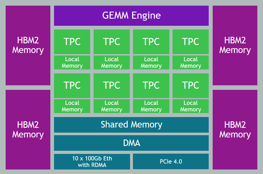
Today I would like to tell you about our new DL1 instances. Powered by Gaudi accelerators from Habana Labs, the dl1.24xlarge instances have the following specs:
Gaudi Accelerators – Each instance is equipped with eight Gaudi accelerators, with a total of 256 GB of High Bandwidth (HBM2) accelerator memory and high-speed, RDMA-powered communication between accelerators.
System Memory – 768 GB of system memory, enough to hold very large sets of training data in memory, as often requested by our customers.
Local Storage – 4 TB of local NVMe storage, configured as four 1 TB volumes.
Processor – Intel Cascade Lake processor with 96 vCPUs.
Network – 400 Gbps of network throughput.
As you can see, we have maxed out the specs in just about every dimension, with the goal of giving you a highly capable machine learning training platform with a low cost of entry and up to 40% better price-performance than current GPU-based EC2 instances.
Gaudi Inside
The Gaudi accelerators are custom-designed for machine learning training, and have a ton of cool & interesting features & attributes:
Data Types – Support for floating point (BF16 and FP32), signed integer (INT8, INT16, and INT32), and unsigned integer (UINT8, UINT16, and UINT32) data.
Generalized Matrix Multiplier Engine (GEMM) – Specialized hardware to accelerate matrix multiplication.
Tensor Processing Cores (TPCs) – Specialized VLIW SIMD (Very Long Instruction Word / Single Instruction Multiple Data) processing units designed for ML training. The TPCs are C-programmable, although most users will use higher-level tools and frameworks.
Getting Started with DL1 Instances
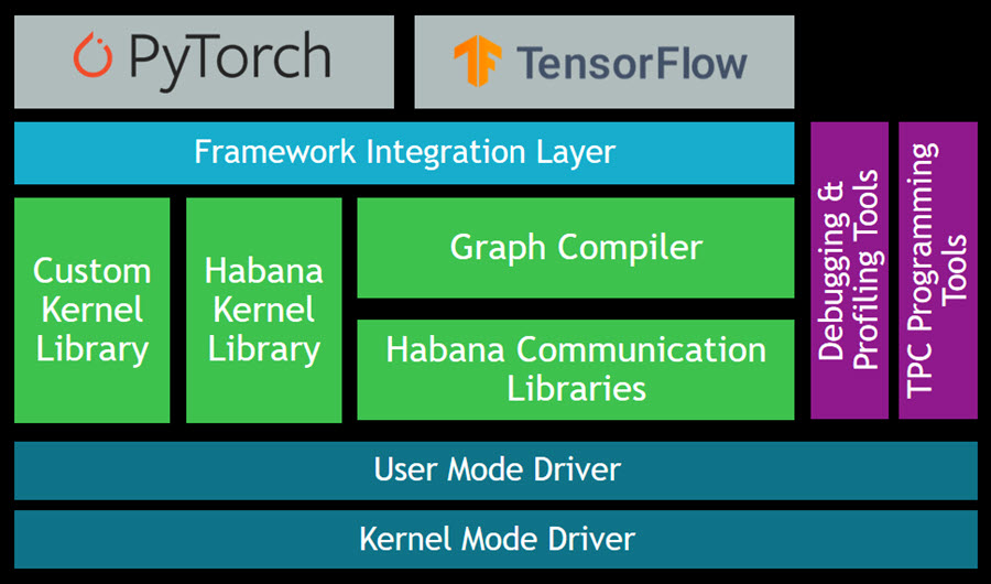
The Gaudi SynapseAI Software Suite for Training will help you to build new models and to migrate existing models from popular frameworks such as PyTorch and TensorFlow:
Here are some resources to get you started:
TensorFlow User Guide – Learn how to run your TensorFlow models on Gaudi.
PyTorch User Guide – Learn how to run your PyTorch models on Gaudi.
Gaudi Model Migration Guide – Learn how to port your PyTorch or TensorFlow to Gaudi.
HabanaAI Repo – This large, active repo contains setup instructions, reference models, academic papers, and much more.
You can use the TPC Programming Tools to write, simulate, and debug code that runs directly on the TPCs, and you can use the Habana Communication Library (HCL) to build applications that harness the power of multiple accelerators. The Habana Collective Communications Library (HCCL) runs atop HCL and gives you access to collective primitives for Reduce, Broadcast, Gather, and Scatter operations.
Now Available
DL1 instances are available today in the US East (N. Virginia) and US West (Oregon) Regions in On-Demand and Spot form. You can purchase Reserved Instances and Savings plans as well.
— Jeff;
AWS Local Zones Are Now Open in Las Vegas, New York City, and Portland
Post Syndicated from Sébastien Stormacq original https://aws.amazon.com/blogs/aws/aws-local-zones-are-now-open-in-las-vegas-new-york-city-and-portland/
Today, we are opening three new AWS Local Zones in Las Vegas, New York City (located in New Jersey), and Portland metro areas. We are now at a total of 14 Local Zones in 13 cities since Jeff Barr announced the first Local Zone in Los Angeles in December 2019. These three new Local Zones join the ones in full operation in Boston, Chicago, Dallas, Denver, Houston, Kansas City, Los Angeles, Miami, Minneapolis, and Philadelphia.
Local Zones are one of the ways we bring select AWS services much closer to large populations and geographic areas where major industries come together. By having this proximity, you can deploy latency-sensitive workloads such as real-time gaming platforms, financial transaction processing, media and entertainment content creation, or ad services. Using Local Zones for migrations or hybrid strategies are two additional use cases allowing you to migrate your applications to a nearby AWS Local Zone while still meeting the low-latency requirements of hybrid deployments.
Local Zones support the deployment of workloads using Amazon Elastic Compute Cloud (Amazon EC2), Amazon Elastic Block Store (EBS), Amazon FSx for Windows File Server and Amazon FSx for Lustre, Elastic Load Balancing, Amazon Relational Database Service (RDS), and Amazon Virtual Private Cloud (VPC). Local Zones provide a high-bandwidth, secure connection between local workloads and those running in the parent AWS Region, while offering the full range of services found in a Region through the same APIs, console and tool sets. This page lists the exact AWS services and features available in each Local Zone.
Local Zones are easy to use and can be enabled in only three clicks! This article will help you learn how to provision infrastructure in a Local Zone, which is very similar to creating infrastructure in an Availability Zone. Once enabled, Local Zones appear as additional Availability Zones in your AWS Management Console or AWS Command Line Interface (CLI).
Local Zones in Action
Examples of workloads that our customers run in Local Zones include:
Dish Wireless is building the US-telecom’s first cloud-native 5G network. They are unleashing 5G connectivity with better speed, better security, and better latency. DISH is leveraging AWS Regions, AWS Local Zones, and AWS Outposts to extend AWS infrastructure and services to wherever they – or their customers – need it.
Integral Ad Science (IAS) is a global leader in digital media quality. Every millisecond counts when it comes to delivering actionable insights for its advertiser and publisher customers. Leveraging AWS Regions and AWS Local Zones, IAS ensures rapid response times in milliseconds when analyzing data and delivering insights.
Esports Engine (a Vindex company) is a turnkey esports solutions company working with gaming publishers, rights holders, brands, and teams to provide production, broadcast, tournament, and program design. Their graphic-intensive streaming content is live-fed from the locations where the games are recorded and then broadcast from the studios to viewers. AWS Local Zones replace their previous on-premises data centers to reduce the need for support for the physical data center buildings.
Proof Trading is a financial services company looking forward to taking advantage of AWS Local Zones to bring trading workloads closer to the major trading venues located in Chicago and New Jersey. Our industry blog has a detailed article that provides more context on trading-related workloads.
Ubitus is a cloud gaming technology leader. They deploy latency-sensitive game servers all over the world to be closer to gamers. An important part of having a great gaming experience is to have consistent low-latency game plays. AWS Local Zones are a game changer for them. Now, they can easily deploy and test clusters of game servers in many cities across the US, ensuring that more customers get a consistent experience regardless of where they are located.
What’s Next?
In 2019 when we launched our first Local Zone at AWS re:Invent 2019, we said we were just getting started. In addition to today’s announcement, we are working on opening three additional Local Zones in Atlanta, Phoenix, and Seattle by the end of the year, and we keep expanding. If you would like to express your interest in a particular location, please let us know by filling out the AWS Local Zones Interest form.
We are also listening to your feedback on additional services that we should add to Local Zones, such as more EC2 instance types to give you even more flexibility.
Build and deploy your workload on a Local Zone today.
Automate building an integrated analytics solution with AWS Analytics Automation Toolkit
Post Syndicated from Manash Deb original https://aws.amazon.com/blogs/big-data/automate-building-an-integrated-analytics-solution-with-aws-analytics-automation-toolkit/
Amazon Redshift is a fast, fully managed, widely popular cloud data warehouse that powers the modern data architecture enabling fast and deep insights or machine learning (ML) predictions using SQL across your data warehouse, data lake, and operational databases. A key differentiating factor of Amazon Redshift is its native integration with other AWS services, which makes it easy to build complete, comprehensive, and enterprise-level analytics applications.
As analytics solutions have moved away from the one-size-fits-all model to choosing the right tool for the right function, architectures have become more optimized and performant while simultaneously becoming more complex. You can use Amazon Redshift for a variety of use cases, along with other AWS services for ingesting, transforming, and visualizing the data.
Manually deploying these services is time-consuming. It also runs the risk of making human errors and deviating from best practices.
In this post, we discuss how to automate the process of building an integrated analytics solution by using a simple script.
Solution overview
The framework described in this post uses Infrastructure as Code (IaC) to solve the challenges with manual deployments, by using AWS Cloud Development Kit (CDK) to automate provisioning AWS analytics services. You can indicate the services and resources you want to incorporate in your infrastructure by editing a simple JSON configuration file.
The script then instantly auto-provisions all the required infrastructure components in a dynamic manner, while simultaneously integrating them according to AWS recommended best practices.
In this post, we go into further detail on the specific steps to build this solution.
Prerequisites
Prior to deploying the AWS CDK stack, complete the following prerequisite steps:
- Verify that you’re deploying this solution in a Region that supports AWS CloudShell. For more information, see AWS CloudShell endpoints and quotas.
- Have an AWS Identity and Access Management (IAM) user with the following permissions:
AWSCloudShellFullAccessIAM Full AccessAWSCloudFormationFullAccessAmazonSSMFullAccessAmazonRedshiftFullAccessAmazonS3ReadOnlyAccessSecretsManagerReadWriteAmazonEC2FullAccess- Create a custom AWS Database Migration Service (AWS DMS) policy called
AmazonDMSRoleCustomwith the following permissions:
- Optionally, create a key pair that you have access to. This is only required if deploying the AWS Schema Conversion Tool (AWS SCT).
- Optionally, if using resources outside your AWS account, open firewalls and security groups to allow traffic from AWS. This is only applicable for AWS DMS and AWS SCT deployments.
Prepare the config file
To launch the target infrastructures, download the user-config-template.json file from the GitHub repo.
To prep the config file, start by entering one of the following values for each key in the top section: CREATE, N/A, or an existing resource ID to indicate whether you want to have the component provisioned on your behalf, skipped, or integrated using an existing resource in your account.
For each of the services with the CREATE value, you then edit the appropriate section under it with the specific parameters to use for that service. When you’re done customizing the form, save it as user-config.json.
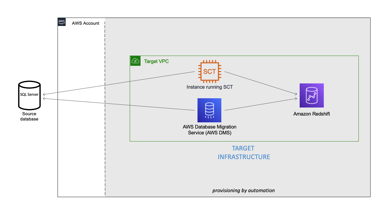
You can see an example of the completed config file under user-config-sample.json in the GitHub repo, which illustrates a config file for the following architecture by newly provisioning all the services, including Amazon Virtual Private Cloud (Amazon VPC), Amazon Redshift, an Amazon Elastic Compute Cloud (Amazon EC2) instance with AWS SCT, and AWS DMS instance connecting an external source SQL Server on Amazon EC2 to the Amazon Redshift cluster.
Launch the toolkit
This project uses CloudShell, a browser-based shell service, to programatically initiate the deployment through the AWS Management Console. Prior to opening CloudShell, you need to configure an IAM user, as described in the prerequisites.
- On the CloudShell console, clone the Git repository:
- Run the deployment script:
- On the Actions menu, choose Upload file and upload
user-config.json.

- Enter a name for the stack.
- Depending on the resources being deployed, you may have to provide additional information, such as the password for an existing database or Amazon Redshift cluster.
- Press Enter to initiate the deployment.

Monitor the deployment
After you run the script, you can monitor the deployment of resource stacks through the CloudShell terminal, or through the AWS CloudFormation console, as shown in the following screenshot.
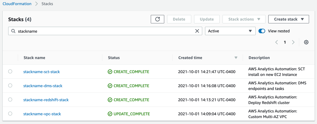
Each stack corresponds to the creation of a resource from the config file. You can see the newly created VPC, Amazon Redshift cluster, EC2 instance running AWS SCT, and AWS DMS instance. To test the success of the deployment, you can test the newly created AWS DMS endpoint connectivity to the source system and the target Amazon Redshift cluster. Select your endpoint and on the Actions menu, choose Test connection.
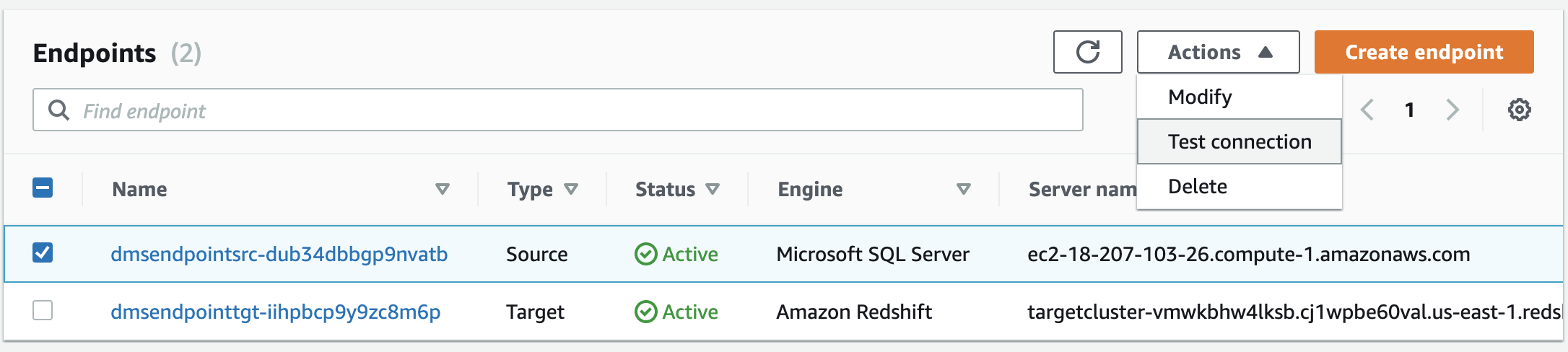
If both statuses say Success, the AWS DMS workflow is fully integrated.
Troubleshooting
If the stack launch stalls at any point, visit our GitHub repository for troubleshooting instructions.
Conclusion
In this post, we discussed how you can use the AWS Analytics Infrastructure Automation utility to quickly get started with Amazon Redshift and other AWS services. It helps you provision your entire solution on AWS instantly without any spending any time on challenges around integrating the services or scaling your solution.
About the Authors
 Manash Deb is a Software Development Engineer in the AWS Directory Service team. He has worked on building end-to-end applications in different database and technologies for over 15 years. He loves to learn new technologies and solving, automating, and simplifying customer problems on AWS.
 Samir Kakli is an Analytics Specialist Solutions Architect at AWS. He has worked with building and tuning databases and data warehouse solutions for over 20 years. His focus is architecting end-to-end analytics solutions designed to meet the specific needs for each customer.
 Julia Beck is a Specialist Solutions Architect at AWS. She supports customers building analytics proof of concept workloads. Outside of work, she enjoys traveling, cooking, and puzzles.
TV or Projector? both. The ULTIMATE Hidden Home Theater Setup!
Post Syndicated from The Hook Up original https://www.youtube.com/watch?v=KgUVGvFRCsk
Accelerate large-scale data migration validation using PyDeequ
Post Syndicated from Mahendar Gajula original https://aws.amazon.com/blogs/big-data/accelerate-large-scale-data-migration-validation-using-pydeequ/
Many enterprises are migrating their on-premises data stores to the AWS Cloud. During data migration, a key requirement is to validate all the data that has been moved from on premises to the cloud. This data validation is a critical step and if not done correctly, may result in the failure of the entire project. However, developing custom solutions to determine migration accuracy by comparing the data between the source and target can often be time-consuming.
In this post, we walk through a step-by-step process to validate large datasets after migration using PyDeequ. PyDeequ is an open-source Python wrapper over Deequ (an open-source tool developed and used at Amazon). Deequ is written in Scala, whereas PyDeequ allows you to use its data quality and testing capabilities from Python and PySpark.
Prerequisites
Before getting started, make sure you have the following prerequisites:
- An AWS account with access to AWS services
- An Amazon Virtual Private Cloud (Amazon VPC) with a public subnet
- An Amazon Elastic Compute Cloud (Amazon EC2) key pair
- An AWS Identity and Access Management (IAM) policy for AWS Secrets Manager permissions
- A SQL editor to connect to the source database
- IAM roles
EMR_DefaultRoleandEMR_EC2_DefaultRoleavailable in your account
Solution overview
This solution uses the following services:
- Amazon RDS for My SQL as the database engine for the source database.
- Amazon Simple Storage Service (Amazon S3) or Hadoop Distributed File System (HDFS) as the target.
- Amazon EMR to run the PySpark script. We use PyDeequ to validate data between MySQL and the corresponding Parquet files present in the target.
- AWS Glue to catalog the technical table, which stores the result of the PyDeequ job.
- Amazon Athena to query the output table to verify the results.
We use profilers, which is one of the metrics computation components of PyDeequ. We use this to analyze each column in the given dataset to calculate statistics like completeness, approximate distinct values, and data types.
The following diagram illustrates the solution architecture.
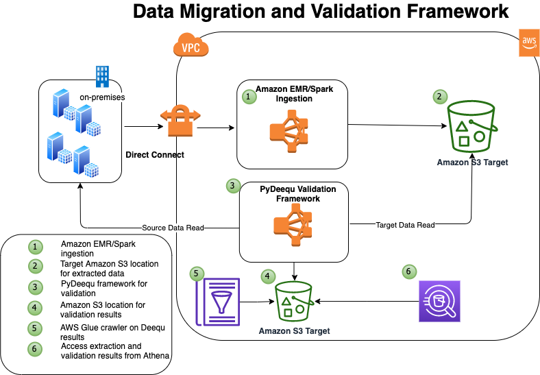
In this example, you have four tables in your on-premises database that you want to migrate: tbl_books, tbl_sales, tbl_venue, and tbl_category.
Deploy the solution
To make it easy for you to get started, we created an AWS CloudFormation template that automatically configures and deploys the solution for you.
The CloudFormation stack performs the following actions:
- Launches and configures Amazon RDS for MySQL as a source database
- Launches Secrets Manager for storing the credentials for accessing the source database
- Launches an EMR cluster, creates and loads the database and tables on the source database, and imports the open-source library for PyDeequ at the EMR primary node
- Runs the Spark ingestion process from Amazon EMR, connecting to the source database, and extracts data to Amazon S3 in Parquet format
To deploy the solution, complete the following steps:
- Choose Launch Stack to launch the CloudFormation template.

The template is launched in the US East (N. Virginia) Region by default.
- On the Select Template page, keep the default URL for the CloudFormation template, then choose Next.
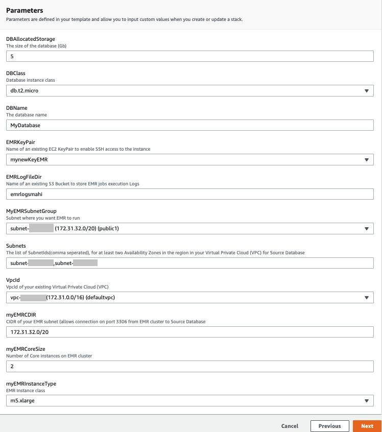
- On the Specify Details page, provide values for the parameters that require input (see the following screenshot).
- Choose Next.

- Choose Next again.
- On the Review page, select I acknowledge that AWS CloudFormation might create IAM resources with custom names.
- Choose Create stack.
You can view the stack outputs on the AWS Management Console or by using the following AWS Command Line Interface (AWS CLI) command:
It takes approximately 20–30 minutes for the deployment to complete. When the stack is complete, you should see the resources in the following table launched and available in your account.
| Resource Name | Functionality |
| DQBlogBucket | The S3 bucket that stores the migration accuracy results for the AWS Glue Data Catalog table |
| EMRCluster | The EMR cluster to run the PyDeequ validation process |
| SecretRDSInstanceAttachment | Secrets Manager for securely accessing the source database |
| SourceDBRds | The source database (Amazon RDS) |
When the EMR cluster is launched, it runs the following steps as part of the post-cluster launch:
- DQsetupStep – Installs the Deequ JAR file and MySQL connector. This step also installs Boto3 and the PyDeequ library. It also downloads sample data files to use in the next step.
- SparkDBLoad – Runs the initial data load to the MySQL database or table. This step creates the test environment that we use for data validation purposes. When this step is complete, we have four tables with data on MySQL and respective data files in Parquet format on HDFS in Amazon EMR.

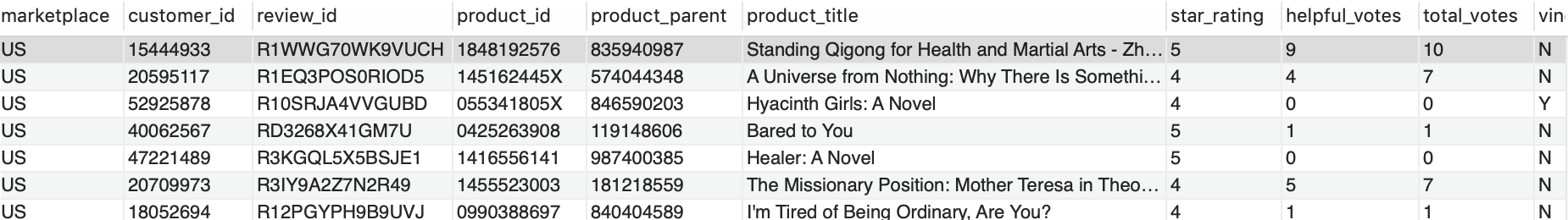
When the Amazon EMR step SparkDBLoad is complete, we verify the data records in the source tables. You can connect to the source database using your preferred SQL editor. For more details, see Connecting to a DB instance running the MySQL database engine.
The following screenshot is a preview of sample data from the source table MyDatabase.tbl_books.
Validate data with PyDeequ
Now the test environment is ready and we can perform data validation using PyDeequ.
- Use Secure Shell (SSH) to connect to the primary node.
- Run the following Spark command, which performs data validation and persists the results to an AWS Glue Data Catalog table (
db_deequ.db_migration_validation_result):
The script and JAR file are already available on your primary node if you used the CloudFormation template. The PySpark script computes PyDeequ metrics on the source MySQL table data and target Parquet files in Amazon S3. The metrics currently calculated as part of this example are as follows:
- Completeness to measure fraction of not null values in a column
- Approximate number of distinct values
- Data type of column
If required, we can compute more metrics for each column. To see the complete list of supported metrics, see the PyDeequ package on GitHub.
The output metrics from the source and target are then compared using a PySpark DataFrame.
When that step is complete, the PySpark script creates the AWS Glue table db_deequ.db_migration_validation_result in your account, and you can query this table from Athena to verify the migration accuracy.
Verify data validation results with Athena
You can use Athena to check the overall data validation summary of all the tables. The following query shows you the aggregated data output. It lists all the tables you validated using PyDeequ and how many columns match between the source and target.
The following screenshot shows our results.
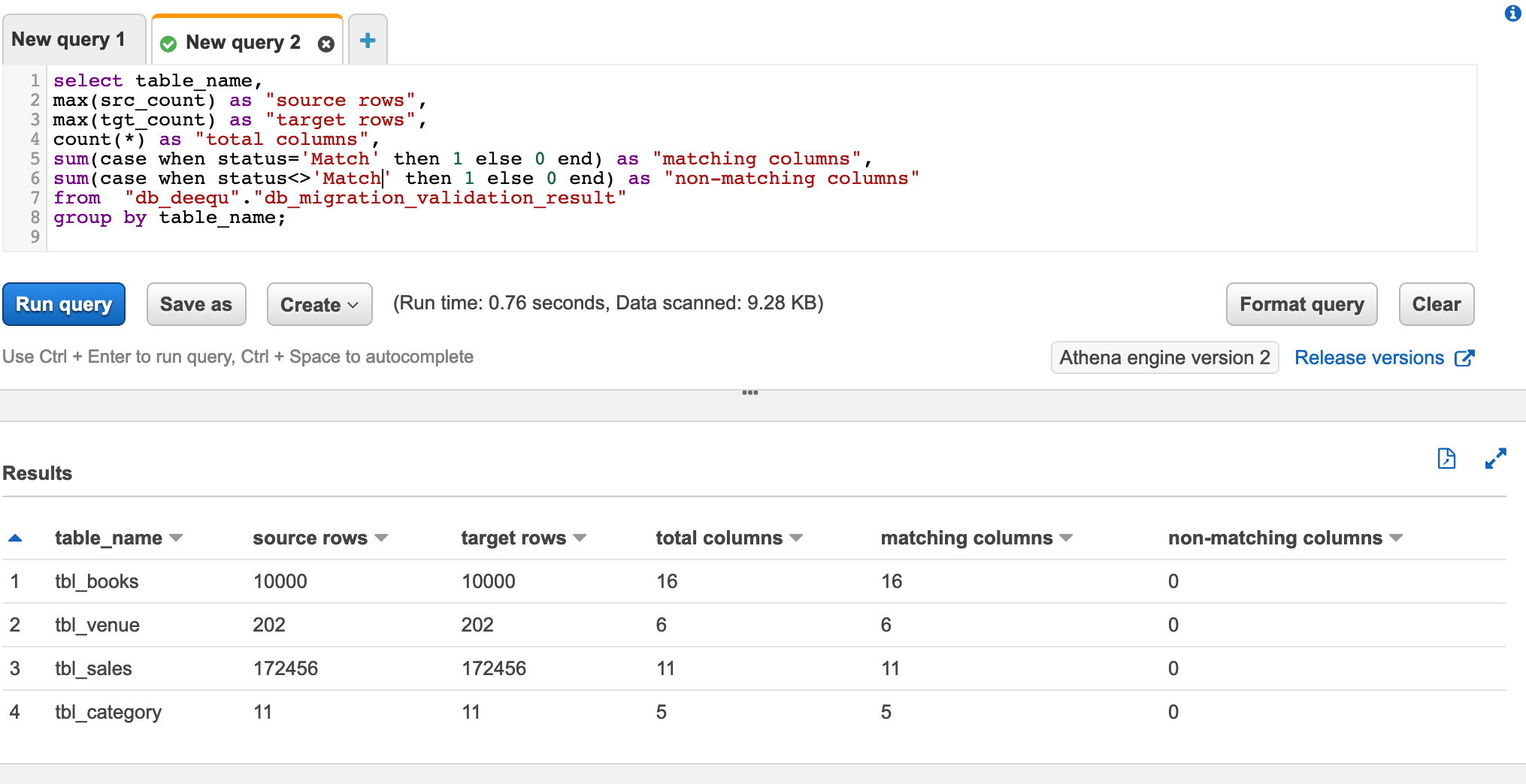
Because all your columns match, you can have high confidence that the data has been exported correctly.
You can also check the data validation report for any table. The following query gives detailed information about any specific table metrics captured as part of PyDeequ validation:
The following screenshot shows the query results. The last column status is the validation result for the columns in the table.
Clean up
To avoid incurring additional charges, complete the following steps to clean up your resources when you’re done with the solution:
- Delete the AWS Glue database and table
db_deequ.db_migration_validation_result. - Delete the prefixes and objects you created from the bucket
dqblogbucket-${AWS::AccountId}. - Delete the CloudFormation stack, which removes your additional resources.
Customize the solution
The solution consists of two parts:
- Data extraction from the source database
- Data validation using PyDeequ
In this section, we discuss ways to customize the solution based on your needs.
Data extraction from the source database
Depending on your data volume, there are multiple ways of extracting data from on-premises database sources to AWS. One recommended service is AWS Data Migration Service (AWS DMS). You can also use AWS Glue, Spark on Amazon EMR, and other services.
In this post, we use PySpark to connect to the source database using a JDBC connection and extract the data into HDFS using an EMR cluster.
The primary reason is that we’re already using Amazon EMR for PyDeequ, and we can use the same EMR cluster for data extraction.
In the CloudFormation template, the Amazon EMR step SparkDBLoad runs the PySpark script blogstep3.py. This PySpark script uses Secrets Manager and a Spark JDBC connection to extract data from the source to the target.
Data validation using PyDeequ
In this post, we use ColumnProfilerRunner from the pydeequ.profiles package for metrics computation. The source data is from the database using a JDBC connection, and the target data is from data files in HDFS and Amazon S3.
To create a DataFrame with metrics information for the source data, use the following code:
Similarly, the metrics is computed for the target (the data file).
You can create a temporary view from the DataFrame to use in the next step for metrics comparison.
After we have both the source (vw_Source) and target (vw_Target) available, we use the following query in Spark to generate the output result:
The generated result is stored in the db_deequ.db_migration_validation_result table in the Data Catalog.
If you used the CloudFormation template, the entire PyDeequ code used in this post is available at the path /home/hadoop/pydeequ_validation.py in the EMR cluster.
You can modify the script to include or exclude tables as per your requirements.
Conclusion
This post showed you how you can use PyDeequ to accelerate the post-migration data validation process. PyDeequ helps you calculate metrics at the column level. You can also use more PyDeequ components like constraint verification to build a custom data validation framework.
For more use cases on Deequ, check out the following:
- Building a serverless data quality and analysis framework with Deequ and AWS Glue
- Build an automatic data profiling and reporting solution with Amazon EMR, AWS Glue, and Amazon QuickSight
- Testing data quality at scale with PyDeequ
About the Authors
 Mahendar Gajula is a Sr. Data Architect at AWS. He works with AWS customers in their journey to the cloud with a focus on Big data, Data Lakes, Data warehouse and AI/ML projects. In his spare time, he enjoys playing tennis and spending time with his family.
 Nitin Srivastava is a Data & Analytics consultant at Amazon Web Services. He has more than a decade of datawarehouse experience along with designing and implementing large scale Big Data and Analytics solutions. He works with customers to deliver the next generation big data analytics platform using AWS technologies.
Amazon RDS Custom for Oracle – New Control Capabilities in Database Environment
Post Syndicated from Channy Yun original https://aws.amazon.com/blogs/aws/amazon-rds-custom-for-oracle-new-control-capabilities-in-database-environment/
Managing databases in self-managed environments such as on premises or Amazon Elastic Compute Cloud (Amazon EC2) requires customers to spend time and resources doing database administration tasks such as provisioning, scaling, patching, backups, and configuring for high availability. So, hundreds of thousands of AWS customers use Amazon Relational Database Service (Amazon RDS) because it automates these undifferentiated administration tasks.
However, there are some legacy and packaged applications that require customers to make specialized customizations to the underlying database and the operating system (OS), such as Oracle industry specialized applications for healthcare and life sciences, telecom, retail, banking, and hospitality. Customers with these specific customization requirements cannot get the benefits of a fully managed database service like Amazon RDS, and they end up deploying their databases on premises or on EC2 instances.
Today, I am happy to announce the general availability of Amazon RDS Custom for Oracle, new capabilities that enable database administrators to access and customize the database environment and operating system. With RDS Custom for Oracle, you can now access and customize your database server host and operating system, for example by applying special patches and changing the database software settings to support third-party applications that require privileged access.
You can easily move your existing self-managed database for these applications to Amazon RDS and automate time-consuming database management tasks, such as software installation, patching, and backups. Here is a simple comparison of features and responsibilities between Amazon EC2, RDS Custom for Oracle, and RDS.
| Features and Responsibilities | Amazon EC2 | RDS Custom for Oracle | Amazon RDS |
| Application optimization | Customer | Customer | Customer |
| Scaling/high availability | Customer | Shared | AWS |
| DB backups | Customer | Shared | AWS |
| DB software maintenance | Customer | Shared | AWS |
| OS maintenance | Customer | Shared | AWS |
| Server maintenance | AWS | AWS | AWS |
The shared responsibility model of RDS Custom for Oracle gives you more control than in RDS, but also more responsibility, similar to EC2. So, if you need deep control of your database environment where you take responsibility for changes that you make and want to offload common administration tasks to AWS, RDS Custom for Oracle is the recommended deployment option over self-managing databases on EC2.
Getting Started with Amazon RDS Custom for Oracle
To get started with RDS Custom for Oracle, you create a custom engine version (CEV), the database installation files of supported Oracle database versions and upload the CEV to Amazon Simple Storage Service (Amazon S3). This launch includes Oracle Enterprise Edition allowing Oracle customers to use their own licensed software with bring your own license (BYOL).
Then with just a few clicks in the AWS Management Console, you can deploy an Oracle database instance in minutes. Then, you can connect to it using SSH or AWS Systems Manager.

Before creating and connecting your DB instance, make sure that you meet some prerequisites such as configuring the AWS Identity and Access Management (IAM) role and Amazon Virtual Private Cloud (VPC) using the pre-created AWS CloudFormation template in the Amazon RDS User Guide.
A symmetric AWS Key Management Service (KMS) key is required for RDS Custom for Oracle. If you don’t have an existing symmetric KMS key in your account, create a KMS key by following the instructions in Creating keys in the AWS KMS Developer Guide.
The Oracle Database installation files and patches are hosted on Oracle Software Delivery Cloud. If you want to create a CEV, search and download your preferred version under the Linux x86/64 platform and upload it to Amazon S3.
$ aws s3 cp install-or-patch-file.zip \ s3://my-oracle-db-filesTo create CEV for creating a DB instance, you need a CEV manifest, a JSON document that describes installation .zip files stored in Amazon S3. RDS Custom for Oracle will apply the patches in the order in which they are listed when creating the instance by using this CEV.
{
    "mediaImportTemplateVersion": "2020-08-14",
    "databaseInstallationFileNames": [
        "V982063-01.zip"
    ],
    "opatchFileNames": [
        "p6880880_190000_Linux-x86-64.zip"
    ],
    "psuRuPatchFileNames": [
        "p32126828_190000_Linux-x86-64.zip"
    ],
    "otherPatchFileNames": [
        "p29213893_1910000DBRU_Generic.zip",
        "p29782284_1910000DBRU_Generic.zip",
        "p28730253_190000_Linux-x86-64.zip",
        "p29374604_1910000DBRU_Linux-x86-64.zip",
        "p28852325_190000_Linux-x86-64.zip",
        "p29997937_190000_Linux-x86-64.zip",
        "p31335037_190000_Linux-x86-64.zip",
        "p31335142_190000_Generic.zip"
] }
To create a CEV in the AWS Management Console, choose Create custom engine version in the Custom engine version menu.

You can set Engine type to Oracle, choose your preferred database edition and version, and enter CEV manifest, the location of the S3 bucket that you specified. Then, choose Create custom engine version. Creation takes approximately two hours.

To create your DB instance with the prepared CEV, choose Create database in the Databases menu. When you choose a database creation method, select Standard create. You can set Engine options to Oracle and choose Amazon RDS Custom in the database management type.

In Settings, enter a unique name for the DB instance identifier and your master username and password. By default, the new instance uses an automatically generated password for the master user. To learn more in the remaining setting, see Settings for DB instances in the Amazon RDS User Guide. Choose Create database.
Alternatively, you can create a CEV by running create-custom-db-engine-version command in the AWS Command Line Interface (AWS CLI).
$ aws rds create-db-instances \
      --engine my-oracle-ee \
      --db-instance-identifier my-oracle-instance \
      --engine-version 19.my_cev1 \
      --allocated-storage 250 \
      --db-instance-class db.m5.xlarge \
      --db-subnet-group mydbsubnetgroup \
      --master-username masterawsuser \
      --master-user-password masteruserpassword \
      --backup-retention-period 3 \
      --no-multi-az \
              --port 8200 \
      --license-model bring-your-own-license \
      --kms-key-id my-kms-key
After you create your DB instance, you can connect to this instance using an SSH client. The procedure is the same as for connecting to an Amazon EC2 instance. To connect to the DB instance, you need the key pair associated with the instance. RDS Custom for Oracle creates the key pair on your behalf. The pair name uses the prefix do-not-delete-ssh-privatekey-db-. AWS Secrets Manager stores your private key as a secret.

For more information, see Connecting to your Linux instance using SSH in the Amazon EC2 User Guide.
You can also connect to it using AWS Systems Manager Session Manager, a capability that lets you manage EC2 instances through a browser-based shell. To learn more, see Connecting to your RDS Custom DB instance using SSH and AWS Systems Manager in the Amazon RDS User Guide.
Things to Know
Here are a couple of things to keep in mind about managing your DB instance:
High Availability (HA): To configure replication between DB instances in different Availability Zones to be resilient to Availability Zone failures, you can create read replicas for RDS Custom for Oracle DB instances. Read replica creation is similar to Amazon RDS, but with some differences. Not all options are supported when creating RDS Custom read replicas. To learn how to configure HA, see Working with RDS Custom for Oracle read replicas in the AWS Documentation.
Backup and Recovery: Like Amazon RDS, RDS Custom for Oracle creates and saves automated backups during the backup window of your DB instance. You can also back up your DB instance manually. The procedure is identical to taking a snapshot of an Amazon RDS DB instance. The first snapshot contains the data for the full DB instance just like in Amazon RDS. RDS Custom also includes a snapshot of the OS image, and the EBS volume that contains the database software. Subsequent snapshots are incremental. With backup retention enabled, RDS Custom also uploads transaction logs into an S3 bucket in your account to be used with the RDS point-in-time recovery feature. Restore DB snapshots, or restore DB instances to a specific point in time using either the AWS Management Console or the AWS CLI. To learn more, see Backing up and restoring an Amazon RDS Custom for Oracle DB instance in the Amazon RDS User Guide.
Monitoring and Logging: RDS Custom for Oracle provides a monitoring service called the support perimeter. This service ensures that your DB instance uses a supported AWS infrastructure, operating system, and database. Also, all changes and customizations to the underlying operating system are automatically logged for audit purposes using Systems Manager and AWS CloudTrail. To learn more, see Troubleshooting an Amazon RDS Custom for DB instance in the Amazon RDS User Guide.
Now Available
Amazon RDS Custom for Oracle is now available in US East (N. Virginia), US East (Ohio), US West (Oregon), EU (Frankfurt), EU (Ireland), EU (Stockholm), Asia Pacific (Singapore), Asia Pacific (Sydney), and Asia Pacific (Tokyo) regions.
To learn more, take a look at the product page and documentations of Amazon RDS Custom for Oracle. Please send us feedback either in the AWS forum for Amazon RDS or through your usual AWS support contacts.
– Channy
Three ways to improve your cybersecurity awareness program
Post Syndicated from Stephen Schmidt original https://aws.amazon.com/blogs/security/three-ways-to-improve-your-cybersecurity-awareness-program/
Raising the bar on cybersecurity starts with education. That’s why we announced in August that Amazon is making its internal Cybersecurity Awareness Training Program available to businesses and individuals for free starting this month. This is the same annual training we provide our employees to help them better understand and anticipate potential cybersecurity risks. The training program will include a getting started guide to help you implement a cybersecurity awareness training program at your organization. It’s aligned with NIST SP 800-53rev4, ISO 27001, K-ISMS, RSEFT, IRAP, OSPAR, and MCTS.
I also want to share a few key learnings for how to implement effective cybersecurity training programs that might be helpful as you develop your own training program:
- Be sure to articulate personal value. As humans, we have an evolved sense of physical risk that has developed over thousands of years. Our bodies respond when we sense danger, heightening our senses and getting us ready to run or fight. We have a far less developed sense of cybersecurity risk. Your vision doesn’t sharpen when you assign the wrong permissions to a resource, for example. It can be hard to describe the impact of cybersecurity, but if you keep the message personal, it engages parts of the brain that are tied to deep emotional triggers in memory. When we describe how learning a behavior—like discerning when an email might be phishing—can protect your family, your child’s college fund, or your retirement fund, it becomes more apparent why cybersecurity matters.
- Be inclusive. Humans are best at learning when they share a lived experience with their educators so they can make authentic connections to their daily lives. That’s why inclusion in cybersecurity training is a must. But that only happens by investing in a cybersecurity awareness team that includes people with different backgrounds, so they can provide insight into different approaches that will resonate with diverse populations. People from different cultures, backgrounds, and age cohorts can provide insight into culturally specific attack patterns as well as how to train for them. For example, for social engineering in hierarchical cultures, bad actors often spoof authority figures, and for individualistic cultures, they play to the target’s knowledge and importance, and give compliments. And don’t forget to make everything you do accessible for people with varying disability experiences, because everyone deserves the same high-quality training experience. The more you connect with people, the more they internalize your message and provide valuable feedback. Diversity and inclusion breeds better cybersecurity.
- Weave it into workflows. Training takes investment. You have to make time for it in your day. We all understand that as part of a workforce we have to do it, but in addition to compliance training, you should be providing just-in-time reminders and challenges to complete. Try working with tooling teams to display messaging when critical tasks are being completed. Make training short and concise—3 minutes at most—so that people can make time for it in their day.
Cybersecurity training isn’t just a once-per-year exercise. Find ways to weave it into the daily lives of your workforce, and you’ll be helping them protect not only your company, but themselves and their loved ones as well.
Get started by going to learnsecurity.amazon.com and take the Cybersecurity Awareness training.
Want more AWS Security how-to content, news, and feature announcements? Follow us on Twitter.
19 – ClearlyIP SIP Trunking – FreePBX 101 v15
Post Syndicated from Crosstalk Solutions original https://www.youtube.com/watch?v=_0pgUUIsM00
Drive Failure Over Time: The Bathtub Curve Is Leaking
Post Syndicated from original https://www.backblaze.com/blog/drive-failure-over-time-the-bathtub-curve-is-leaking/
From time to time, we will reference the “bathtub curve” when talking about hard drive and SSD failure rates. This normally includes a reference or link back to a post we did in 2013 which discusses the topic. It’s time for an update. Not because the bathtub curve itself has changed, but because we have nearly seven times the number of drives and eight more years of data than we did in 2013.
In today’s post, we’ll take an updated look at how well hard drive failure rates fit the bathtub curve, and in a few weeks we’ll delve into the specifics for different drive models and even do a little drive life expectancy analysis.
Once Upon a Time, There Was a Bathtub Curve
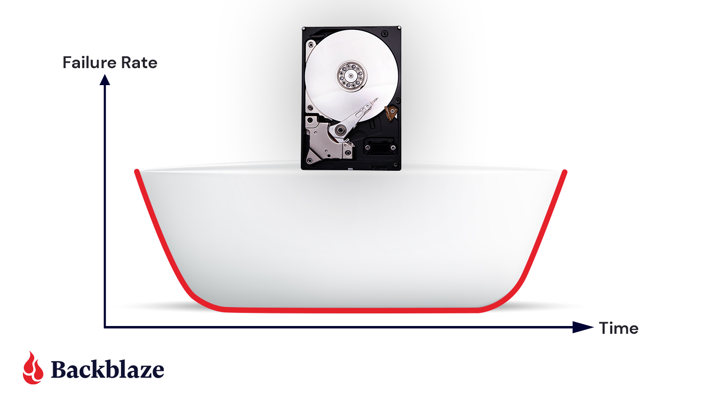
Here is the classic version of the bathtub curve.
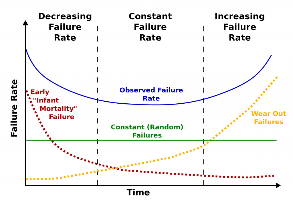
The curve is divided into three sections: decreasing failure rate, constant failure rate, and increasing failure rate. Using our 2013 drive stats data, we computed a failure rate and a timeframe for each of the three sections as follows:
2013 Drive Failure Rates
| Curve Section | Failure Rate | Length |
|---|---|---|
| Decreasing | 5.1% | 0 to 18 Months |
| Constant | 1.4% | 18 Months to 3 Years |
| Increasing | 11.8% | 3 to 4 Years |
Furthermore, we computed that at four years, the life expectancy of a hard drive in our system was about 80%, and forecasting that out, at six years, the life expectancy was 50%. In other words, we would expect a hard drive we installed to have a 50% chance of being alive after six years.
Drive Failure and the Bathtub Curve Today
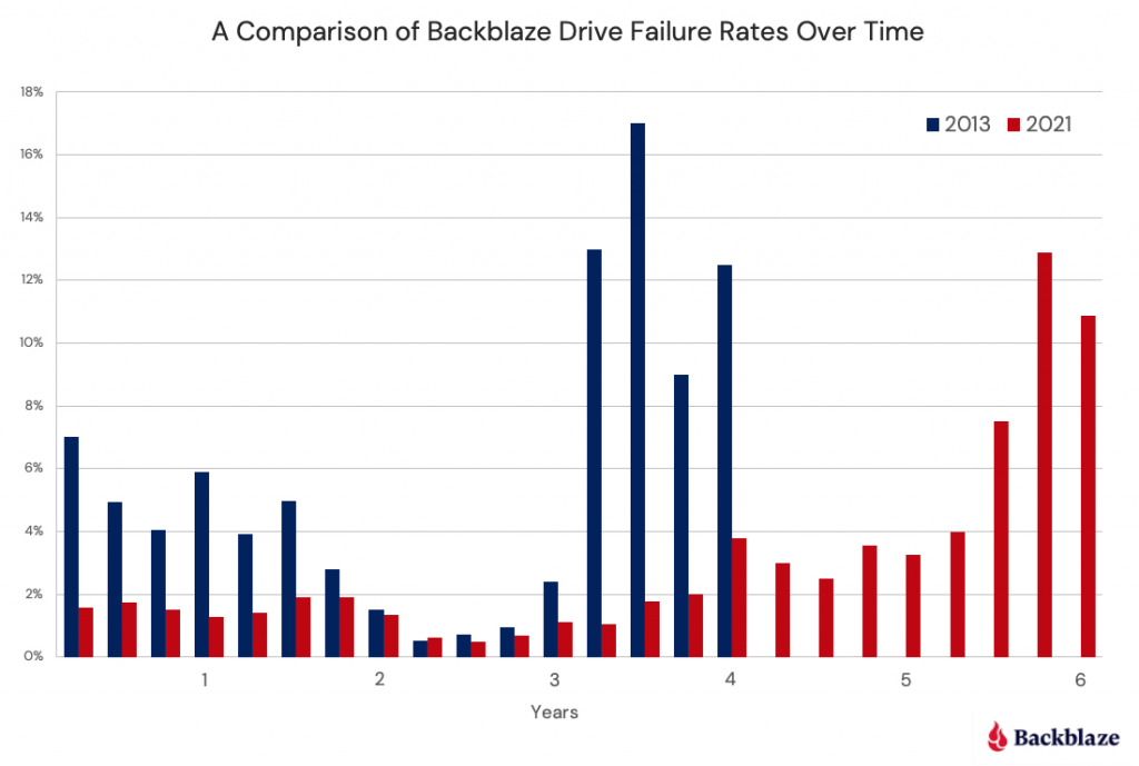
Let’s begin by comparing the drive failure rates over time based on the data available to us in 2013 and the data available to us today in 2021.
Observations and Thoughts
- Let’s start with an easy one: We have six years worth of data for 2021 versus four years for 2013. We have a wider bathtub. In reality, it is even wider, as we have more than six years of data available to us, but after six years the number of data points (drive failures) is small, less than 10 failures per quarter.
- The left side of the bathtub, the area of “decreasing failure rate,” is dramatically lower in 2021 than in 2013. In fact, for our 2021 curve, there is almost no left side of the bathtub, making it hard to take a bath, to say the least. We have reported how Seagate breaks in and tests their newly manufactured hard drives before shipping in an effort to lower the failure rates of their drives. Assuming all manufacturers do the same, that may explain some or all of this observation.
- The right side of the bathtub, the area of “increasing failure rate,” moves right in 2021. Obviously, drives installed after 2013 are not failing as often in years three and four, or most of year five for that matter. We think this may have something to do with the aftermath of the Thailand drive crisis back in 2011. Drives got expensive, and quality (in the form of reduced warranty periods) went down. In addition, there was a fair amount of manufacturer consolidation as well.
- It is interesting that for year two, the two curves, 2013 and 2021, line up very well. We think this is so because there really is a period in the middle in which the drives just work. It was just shorter in 2013 due to the factors noted above.
The Life Expectancy of Drives Today
As noted earlier, back in 2013, the 80% of the drives installed would be expected to survive four years. That fell to 50% after six years. In 2021, the life expectancy of a hard drive being alive at six years is 88%. That’s a substantial increase, but it basically comes down to the fact that hard drives are failing less in our system. We think it is a combination of better drives, better storage servers, and better practices by our data center teams.
What’s Next
For 2021, our bathtub curve looks more like a hockey stick, although saying, “When you review our hockey stick curve…” doesn’t sound quite right. We’ll try to figure out something by our next post on the topic. One thing we also want to do in that next post is to break down the drive failure data by model and see if the different drive models follow the bathtub curve, the hockey stick curve, or some other unnamed curve. We’ll also chart out the life expectancy curves for all the drives as a whole and by drive model as well.
Well, time to get back to the data, our next Drive Stats report is coming up soon.
The post Drive Failure Over Time: The Bathtub Curve Is Leaking appeared first on Backblaze Blog | Cloud Storage & Cloud Backup.
18 – Crosstalk SIP Trunking – FreePBX 101 v15
Post Syndicated from Crosstalk Solutions original https://www.youtube.com/watch?v=pKDK44TiZNo
Interpreting A/B test results: false negatives and power
Post Syndicated from Netflix Technology Blog original https://netflixtechblog.com/interpreting-a-b-test-results-false-negatives-and-power-6943995cf3a8
Martin Tingley with Wenjing Zheng, Simon Ejdemyr, Stephanie Lane, and Colin McFarland
This is the fourth post in a multi-part series on how Netflix uses A/B tests to inform decisions and continuously innovate on our products. Need to catch up? Have a look at Part 1 (Decision Making at Netflix), Part 2 (What is an A/B Test?), Part 3 (False positives and statistical significance). Subsequent posts will go into more details on experimentation across Netflix, how Netflix has invested in infrastructure to support and scale experimentation, and the importance of the culture of experimentation within Netflix.
In Part 3: False positives and statistical significance, we defined the two types of mistakes that can occur when interpreting test results: false positives and false negatives. We then used simple thought exercises based on flipping coins to build intuition around false positives and related concepts such as statistical significance, p-values, and confidence intervals. In this post, we’ll do the same for false negatives and the related concept of statistical power.

False negatives and power
A false negative occurs when the data do not indicate a meaningful difference between treatment and control, but in truth there is a difference. Continuing on an example from Part 3, a false negative corresponds to labeling the photo of the cat as a “not cat.” False negatives are closely related to the statistical concept of power, which gives the probability of a true positive given the experimental design and a true effect of a specific size. In fact, power is simply one minus the false negative rate.
Power involves thinking about possible outcomes given a specific assumption about the actual state of the world — similar to how in Part 3 we defined significance by first assuming the null hypothesis is true. To build intuition about power, let’s go back to the same coin example from Part 3, where the goal is to decide if the coin is unfair using an experiment that calculates the fraction of heads in 100 flips. The distribution of outcomes under the null hypothesis that the coin is fair is shown in black in Figure 2. To make the diagram easier to interpret, we’ve smoothed over the tops of the histograms.
What would happen in this experiment if the coin is not fair? To make the thought exercise more specific, let’s work through what happens when we have a coin where heads occurs, on average, 64% of the time (the choice of that peculiar number will become clear later on). Because there is uncertainty or noise in our experiment, we don’t expect to see exactly 64 heads in 100 flips. But as with the null hypothesis that the coin is fair, we can calculate all the possible outcomes if this specific alternative hypothesis is true. This distribution is shown with the red curve in Figure 2.
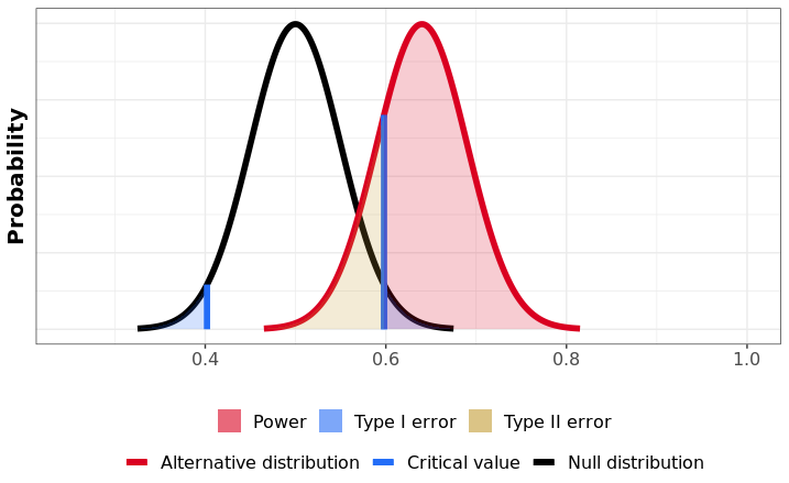
Visually, power is the fraction of this alternative (red) distribution that lies beyond the critical values under the null hypothesis (the blue lines and black curve; see Part 3). Here, 80% of the alternative distribution (red) falls to the right of the taller blue line that demarcates the critical value of the upper rejection region. Assuming that the truth about the coin is that the probability of heads is 64%, then the power of this test is 80%. To be complete, there is also a negligibly small part of the alternative (red) distribution that falls within the lower rejection region (to the left of the short blue line).
The power of a test corresponds to a specific, postulated effect size. In our example, the test has 80% power to detect that a coin is unfair, if that unfair coin in truth has a probability of heads equal to 64%. The interpretation is as follows: if the coin has probability of heads equal to 64%, and we repeatedly run the experiment of flipping 100 times and making a decision at the 5% significance level, then we will correctly reject the null hypothesis that the coin is fair in about 4 out of every 5 experiments. And 20% of those repeated experiments will result in a false negative: we’ll not reject the null hypothesis that the coin is fair, even though it is unfair.
Ways to increase power
In designing an A/B test, we first fix the significance level (the convention is 5%: if there is no difference between treatment and control, we’ll see false positives 5% of the time), and then design the experiment to control false negatives. There are three primary levers we can pull to increase power and reduce the probability of false negatives:
- Effect size. Simply put, the larger the effect size — the difference in metric values between Groups A and B — the higher the probability that we’ll be able to correctly detect that difference. To build intuition, think about running an experiment to determine if a coin is unfair, where the data we collect is the fraction of heads in 100 flips. Now think of two scenarios. In the first scenario, the true probability of heads is 55%, and in the second it is 75%. Intuitively (and mathematically!) it is more likely that our experiment identifies the coin as unfair in the second scenario. The true probability of heads is further from the null value of 50%, so it’s more likely that an experiment will produce an outcome that falls in the rejection region. In the product development context, we can increase the expected magnitude of metric movements by being bold vs incremental with the hypotheses we test. Another strategy to increase effect sizes is to test in new areas of the product, where there may be room for larger improvements in member satisfaction. That said, one of the joys of learning through experimentation is the element of surprise: at times, seemingly small changes can have a major impact on top-line metrics.
- Sample size. The more units in the experiment, the higher the power and the easier it is to correctly identify smaller effects. To build intuition, think again about running an experiment to determine if a coin is unfair, where the data we collect is the fraction of heads in a fixed number of flips and the true probability of heads is 64%. Consider two scenarios: in the first, we flip the coin 20 times, and in the second, we flip the coin 100 times. Intuitively (and mathematically!), it is more likely that our experiment identifies the coin as unfair in the second scenario. With more data, the result from the experiment is going to be closer to the true rate of 64% heads, while the outcomes under the assumption of a fair coin concentrate around 0.50, causing the rejection region to encroach on the 50% value. These effects combine, so that with more data there is a greater probability that the result from the experiment with the unfair coin will fall in that rejection region, resulting in a true positive. In the product development context, we can increase the power by allocating more members (or other units) to the test or by reducing the number of test groups, though there is a tradeoff between the sample size in each test and the number of non-overlapping tests that can be run at the same time.
- The variability of the metric in the underlying population. The more homogenous the metric within the population we are testing on, the easier it is to correctly identify true effects. The intuition for this one is a bit trickier, and our simple coin examples finally break down. Say at Netflix that we run a test that aims to reduce some measure of latency, such as the delay between a member pressing play and video playback commencing. Given the variety of devices and internet connections that people use to access Netflix, there is a lot of natural variability in this metric across our users. As a result, if the test treatment results in a small reduction in the latency metric, it’s hard to successfully identify — the “noise” from the variability across members overwhelms the small signal. In contrast, if we ran the test on a set of members that used similar devices with similar web connections, then the small signal is easier to identify — there is less noise that might drown out the signal. We spend a lot of time at Netflix building statistical analysis models that exploit this intuition, and increase power by effectively lowering the variability; see here for a technical description of our approach.
Powering for reasonable and meaningful effects
Power and the false negative rate are functions of a postulated effect size. Much like how the 5% false positive rate is a widely-accepted convention, the rule of thumb with power is to aim for 80% power for a reasonable and meaningful effect size (we’ll get to each of those below). That is, we postulate an effect size and then design the experiment, primarily through setting the sample size, such that, if the true impact of the treatment experience is as we’ve postulated, the test will correctly identify that there is an effect 80% of the time. And 20% of the time the result from the test will be a false negative: in truth, there is an effect, but our observation from the test does not lie in the rejection region and we fail to conclude that there is an effect. That’s why the examples above used a 64% probability of heads: an experiment with 100 flips then has 80% power.
What constitutes a reasonable effect size can be tricky, as tests can surprise us. But a mix of domain knowledge and common sense can generally provide solid estimates. In an area where testing has a long history, such as optimizing the recommendation systems that help Netflix members choose content that’s great for them, we have a solid idea about the effect sizes that our tests tend to produce (be they positive or negative). Given an understanding of past effect sizes, as well as the analysis strategy, we can set the sample size to ensure the test has 80% power for a reasonable metric movement.
The second consideration, both in this experimental design phase and in deciding where to invest efforts, is to determine what constitutes a meaningful impact to the primary metrics used to decide the test. What is meaningful will depend on the impact area of the experiment (member satisfaction, playback latency, technical performance of back end systems, etc.), and potentially the effort or costs associated with the new product experience. As a hypothetical, say that, for effect sizes smaller than a 0.1% change in the primary metric, the cost of supporting the new product feature outweighs the benefits. In this case, there’s little point in powering a test to detect a 0.01% change in the metric, as successfully identifying an effect of that size won’t result in a meaningful change in decisions. Likewise, if the effect sizes seen in tests in a given innovation area are consistently immaterial to the user experience or the business, that’s a sign that experimentation resources can be more efficiently deployed elsewhere.
Summary
Parts 3 and 4 of this series have focussed on defining and building intuition around the core concepts used to analyze test results: false positives and negatives, statistical significance, p-values, and power.
An uncomfortable truth about experimentation is that we can’t simultaneously minimize both false positives and false negatives. In fact, false positives and negatives trade off with one another. If we used a more stringent false positive rate, such as 0.01%, we’d reduce the number of false positives for tests where there is no difference between A and B — but we’d also reduce the power of the test, increasing the rate of false negatives, for those tests where there is a meaningful difference. Using a 5% false positive rate and targeting 80% power are well-established conventions that balance between limiting false discovery and enabling true discovery. However, in instances where a false positive (or false negative) poses a larger risk, researchers may deviate from these rules of thumb to minimize one type of uncertainty over another.
Our goal is not to eliminate uncertainty, but to understand and quantify the uncertainty in order to make sound decisions. In many cases, results from A/B tests require nuanced interpretation, and in fact the test result itself is only one input into a business decision. In the next post, we’ll cover how to build confidence in a decision using test results. Follow the Netflix Tech Blog to stay up to date.
![]()
Interpreting A/B test results: false negatives and power was originally published in Netflix TechBlog on Medium, where people are continuing the conversation by highlighting and responding to this story.
Security updates for Tuesday
Post Syndicated from original https://lwn.net/Articles/874045/rss
Security updates have been issued by Debian (php7.3 and php7.4), Mageia (kernel and kernel-linus), openSUSE (chromium and virtualbox), Oracle (xstream), Red Hat (kernel, rh-ruby30-ruby, and samba), and Ubuntu (binutils and mysql-5.7).
Monitoring and tuning federated GraphQL performance on AWS Lambda
Post Syndicated from James Beswick original https://aws.amazon.com/blogs/compute/monitoring-and-tuning-federated-graphql-performance-on-aws-lambda/
This post is written by Krzysztof Lis, Senior Software Development Engineer, IMDb.
Our federated GraphQL at IMDb distributes requests across 19 subgraphs (graphlets). To ensure reliability for customers, IMDb monitors availability and performance across the whole stack. This article focuses on this challenge and concludes a 3-part federated GraphQL series:
- Part 1 presents the migration from a monolithic REST API to a federated GraphQL (GQL) endpoint running on AWS Lambda.
- Part 2 describes schema management in federated GQL systems.
This presents an approach towards performance tuning. It compares graphlets with the same logic and different runtime (for example, Java and Node.js) and shows best practices for AWS Lambda tuning.
The post describes IMDb’s test strategy that emphasizes the areas of ownership for the Gateway and Graphlet teams. In contrast to the legacy monolithic system described in part 1, the federated GQL gateway does not own any business logic. Consequently, the gateway integration tests focus solely on platform features, leaving the resolver logic entirely up to the graphlets.
Monitoring and alarming
Efficient monitoring of a distributed system requires you to track requests across all components. To correlate service issues with issues in the gateway or other services, you must pass and log the common request ID.
Capture both error and latency metrics for every network call. In Lambda, you cannot send a response to the client until all work for that request is complete. As a result, this can add latency to a request.
The recommended way to capture metrics is Amazon CloudWatch embedded metric format (EMF). This scales with Lambda and helps avoid throttling by the Amazon CloudWatch PutMetrics API. You can also search and analyze your metrics and logs more easily using CloudWatch Logs Insights.
Lambda configured timeouts emit a Lambda invocation error metric, which can make it harder to separate timeouts from errors thrown during invocation. By specifying a timeout in-code, you can emit a custom metric to alarm on to treat timeouts differently from unexpected errors. With EMF, you can flush metrics before timing out in code, unlike the Lambda-configured timeout.
Running out of memory in a Lambda function also appears as a timeout. Use CloudWatch Insights to see if there are Lambda invocations that are exceeding the memory limits.
You can enable AWS X-Ray tracing for Lambda with a small configuration change to enable tracing. You can also trace components like SDK calls or custom sub segments.
Gateway integration tests
The Gateway team wants tests to be independent from the underlying data served by the graphlets. At the same time, they must test platform features provided by the Gateway – such as graphlet caching.
To simulate the real gateway-graphlet integration, IMDb uses a synthetic test graphlet that serves mock data. Given the graphlet’s simplicity, this reduces the risk of unreliable graphlet data. We can run tests asserting only platform features with the assumption of stable and functional, improving confidence that failing tests indicate issues with the platform itself.
This approach helps to reduce false positives in pipeline blockages and improves the continuous delivery rate. The gateway integration tests are run against the exposed endpoint (for example, a content delivery network) or by invoking the gateway Lambda function directly and passing the appropriate payload.
The former approach allows you to detect potential issues with the infrastructure setup. This is useful when you use infrastructure as code (IaC) tools like AWS CDK. The latter further narrows down the target of the tests to the gateway logic, which may be appropriate if you have extensive infrastructure monitoring and testing already in place.
Graphlet integration tests
The Graphlet team focuses only on graphlet-specific features. This usually means the resolver logic for the graph fields they own in the overall graph. All the platform features – including query federation and graphlet response caching – are already tested by the Gateway Team.
The best way to test the specific graphlet is to run the test suite by directly invoking the Lambda function. If there is any issue with the gateway itself, it does cause a false-positive failure for the graphlet team.
Load tests
It’s important to determine the maximum traffic volume your system can handle before releasing to production. Before the initial launch and before any high traffic events (for example, the Oscars or Golden Globes), IMDb conducts thorough load testing of our systems.
To perform meaningful load testing, the workload captures traffic logs to IMDb pages. We later replay the real customer traffic at the desired transaction-per-second (TPS) volume. This ensures that our tests approximate real-life usage. It reduces the risk of skewing test results due to over-caching and disproportionate graphlet usage. Vegeta is an example of a tool you can use to run the load test against your endpoint.
Canary tests
Canary testing can also help ensure high availability of an endpoint. The canary produces the traffic. This is a configurable script that runs on a schedule. You configure the canary script to follow the same routes and perform the same actions as a user, which allows you to continually verify the user experience even without live traffic.
Canaries should emit success and failure metrics that you can alarm on. For example, if a canary runs 100 times per minute and the success rate drops below 90% in three consecutive data points, you may choose to notify a technician about a potential issue.
Compared with integration tests, canary tests run continuously and do not require any code changes to trigger. They can be a useful tool to detect issues that are introduced outside the code change. For example, through manual resource modification in the AWS Management Console or an upstream service outage.
Performance tuning
There is a per-account limit on the number of concurrent Lambda invocations shared across all Lambda functions in a single account. You can help to manage concurrency by separating high-volume Lambda functions into different AWS accounts. If there is a traffic surge to any one of the Lambda functions, this isolates the concurrency used to a single AWS account.
Lambda compute power is controlled by the memory setting. With more memory comes more CPU. Even if a function does not require much memory, you can adjust this parameter to get more CPU power and improve processing time.
When serving real-time traffic, Provisioned Concurrency in Lambda functions can help to avoid cold start latency. (Note that you should use max, not average for your auto scaling metric to keep it more responsive for traffic increases.) For Java functions, code in static blocks is run before the function is invoked. Provisioned Concurrency is different to reserved concurrency, which sets a concurrency limit on the function and throttles invocations above the hard limit.
Use the maximum number of concurrent executions in a load test to determine the account concurrency limit for high-volume Lambda functions. Also, configure a CloudWatch alarm for when you are nearing the concurrency limit for the AWS account.
There are concurrency limits and burst limits for Lambda function scaling. Both are per-account limits. When there is a traffic surge, Lambda creates new instances to handle the traffic. “Burst limit = 3000” means that the first 3000 instances can be obtained at a much faster rate (invocations increase exponentially). The remaining instances are obtained at a linear rate of 500 per minute until reaching the concurrency limit.
An alternative way of thinking this is that the rate at which concurrency can increase is 500 per minute with a burst pool of 3000. The burst limit is fixed, but the concurrency limit can be increased by requesting a quota increase.
You can further reduce cold start latency by removing unused dependencies, selecting lightweight libraries for your project, and favoring compile-time over runtime dependency injection.
Impact of Lambda runtime on performance
Choice of runtime impacts the overall function performance. We migrated a graphlet from Java to Node.js with complete feature parity. The following graph shows the performance comparison between the two:

To illustrate the performance difference, the graph compares the slowest latencies for Node.js and Java – the P80 latency for Node.js was lower than the minimal latency we recorded for Java.
Conclusion
There are multiple factors to consider when tuning a federated GQL system. You must be aware of trade-offs when deciding on factors like the runtime environment of Lambda functions.
An extensive testing strategy can help you scale systems and narrow down issues quickly. Well-defined testing can also keep pipelines clean of false-positive blockages.
Using CloudWatch EMF helps to avoid PutMetrics API throttling and allows you to run CloudWatch Logs Insights queries against metric data.
For more serverless learning resources, visit Serverless Land.