Field Notes: Clear Unused AWS SSO Mappings Automatically During AWS Control Tower Upgrades

Post Syndicated from Gaurav Gupta original https://aws.amazon.com/blogs/architecture/field-notes-clear-unused-aws-sso-mappings-automatically-during-aws-control-tower-upgrades/

Increasingly organizations are using AWS Control Tower to manage their multiple accounts as well as an external third-party identity source for their federation needs. Cloud architects who use these external identity sources, needed an automated way to clear the unused maps created by AWS Control Tower landing zone as part of the launch, or during update and repair operations. Though the AWS SSO mappings are inaccessible once the external identity source is configured, customers prefer to clear any unused mappings in the directory.

You can remove the permissions sets and mappings that AWS Control Tower deployment creates in AWS SSO. However, when the landing zone is updated or repaired, the default permission sets and mappings are recreated in AWS SSO. In this blog post, we show you how to use AWS Control Tower Lifecycle events to automatically remove these permission sets and mappings when AWS Control Tower is upgraded or repaired. An AWS Lambda function runs on every upgrade and automatically removes the permission sets and mappings.

Overview of solution

Using this CloudFormation template, you can deploy the solution that automatically removes the AWS SSO permission sets and mappings when you upgrade your AWS Control Tower environment. We use AWS CloudFormation, AWS Lambda, AWS SSO and Amazon CloudWatch services to implement this solution.

Figure 1 - Architecture showing how AWS services are used to automatically remove the AWS SSO permission sets and mappings when you upgrade your AWS Control Tower environment

Figure 1 – Architecture showing how AWS services are used to automatically remove the AWS SSO permission sets and mappings when you upgrade your AWS Control Tower environment

To clear the AWS SSO entities and leave the service enabled with no active mappings, we recommend the following steps. This is mainly for those who do not want to use the default AWS SSO deployed by AWS Control Tower.

  • Log in to the AWS Control Tower Management Account and make sure you are in the AWS Control Tower Home Region.
  • Launch AWS CloudFormation stack, which creates:
    • An AWS Lambda function that:
      • Checks/Delete(s) the permission sets mappings created by AWS Control Tower, and
      • Deletes the permission sets created by AWS Control Tower.
  • An AWS IAM role that is assigned to the preceding AWS Lambda Function with minimum required permissions.
  • An Amazon CloudWatch Event Rule that is invoked upon UpdateLandingZone API and triggers the ClearMappingsLambda Lambda function

Prerequisites

For this walkthrough, you should have the following prerequisites:

  • Administrator access to AWS Control Tower management account

Walkthrough

  1. Log in to the AWS account where AWS Control Tower is deployed.
  2. Make sure you are in the home Region of AWS Control Tower.
  3. Deploy the provided CloudFormation template.
    • Download the CloudFormation template.
    • Select AWS CloudFormation service in the AWS Console
    • Select Create Stack and select With new resources (standard)
    • Upload the template file downloaded in Step 1
    • Enter the stack name and choose Next
    • Use the default values in the next page and choose Next
    • Choose Create Stack

By default, in your AWS Control Tower Landing Zone you will see the permission sets and mappings in your AWS SSO service page as shown in the following screenshots:

Figure 2 – Permission sets created by AWS Control Tower

Figure 3 – Account to Permission set mapping created by AWS Control Tower

Now, you can update the AWS Control Tower Landing Zone which will invoke the Lambda function deployed using the CloudFormation template.

Steps to update/repair Control Tower:

  1. Log in to the AWS account where AWS Control Tower is deployed.
  2. Select Landing zone settings from the left-hand pane of the Control Tower dashboard
  3. Select the latest version as seen in the screenshot below.
  4. Select Repair or Update, whichever option is available.
  5. Select Update Landing Zone.

Figure 4 – Updating AWS Control Tower Landing zone

Once the update is complete, you can go to AWS SSO service page and check that the permission sets and the mappings have been removed as shown in the following screenshots:

Figure 5 -Permission sets cleared automatically after Landing zone update

Figure 6 -Mappings cleared after Landing zone update

Cleaning up

If you are only testing this solution, make sure to delete the CloudFormation template, which will remove the relevant resources to stop incurring charges.

Conclusion

In this post, we provided a solution to clear AWS SSO Permission Sets and Mappings when you upgrade your AWS Control Tower Landing Zone. Remember, AWS SSO permission sets are added every time you upgrade AWS Control Tower Landing Zone. With this this solution you don’t have to manage any settings since the AWS Lambda function runs on every upgrade and removes the permission sets and mappings.

Give it a try and let us know your thoughts in the comments!

Field Notes provides hands-on technical guidance from AWS Solutions Architects, consultants, and technical account managers, based on their experiences in the field solving real-world business problems for customers.

Simplifying Zabbix API workflows with named Zabbix API tokens

Post Syndicated from Arturs Lontons original https://blog.zabbix.com/simplifying-zabbix-api-workflows-with-named-zabbix-api-tokens/16653/

Zabbix API enables you to collect any and all information from your Zabbix instance by using a multitude of API methods. You can even utilize Zabbix API calls in your HTTP items. For example, this can be used to monitor the number of particular sets of metrics and visualize their growth over time. With named Zabbix API tokens, such use cases are a lot more simple to implement.

Before Zabbix 5.4 we had to perform the user.login API call to obtain the authentication token. Once the user session was closed, we had to relog, obtain the new authentication token and use it in the subsequent API calls.

With the pre-defined named Zabbix API tokens, you don’t have to constantly check if the authentication token needs to be updated. Starting from Zabbix 5.4 you can simply create a new named Zabbix API token with an expiration date and use it in your API calls.

Creating a new named Zabbix API token

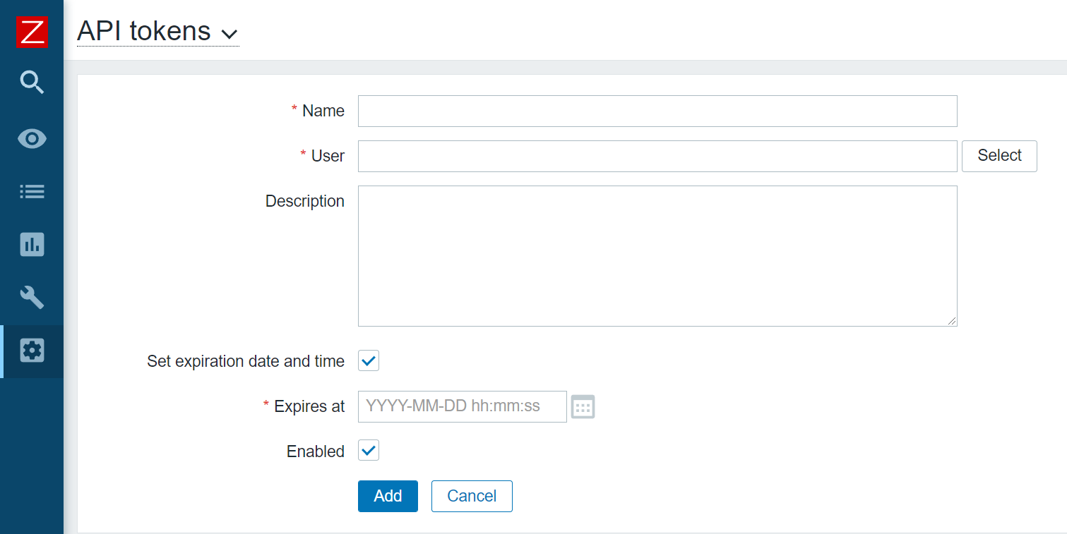
The Zabbix API token creation process is extremely simple. All you have to do is navigate to Administration – General – API tokens and create a new API token. The named API tokens are created for a particular user and can have an optional expiration date and time – otherwise, the tokens are defined without an expiry date.

You can create a named API token in the API tokens section, under Administration – General

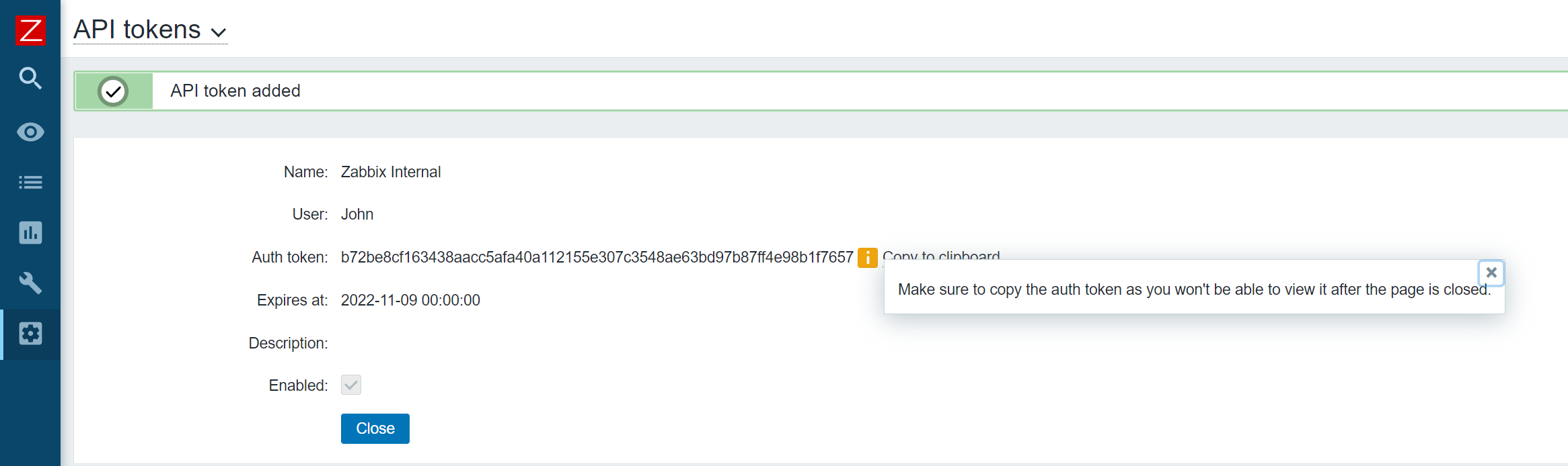
Once the Token has been created, make sure to store it somewhere safe, since you won’t be able to recover it afterward. If the token is lost – you will have to recreate it.

Make sure to store the auth token!

Don’t forget, that when defining a role for the particular API user, we can restrict which API methods this user has access to.

Simplifying API tasks with the named API token

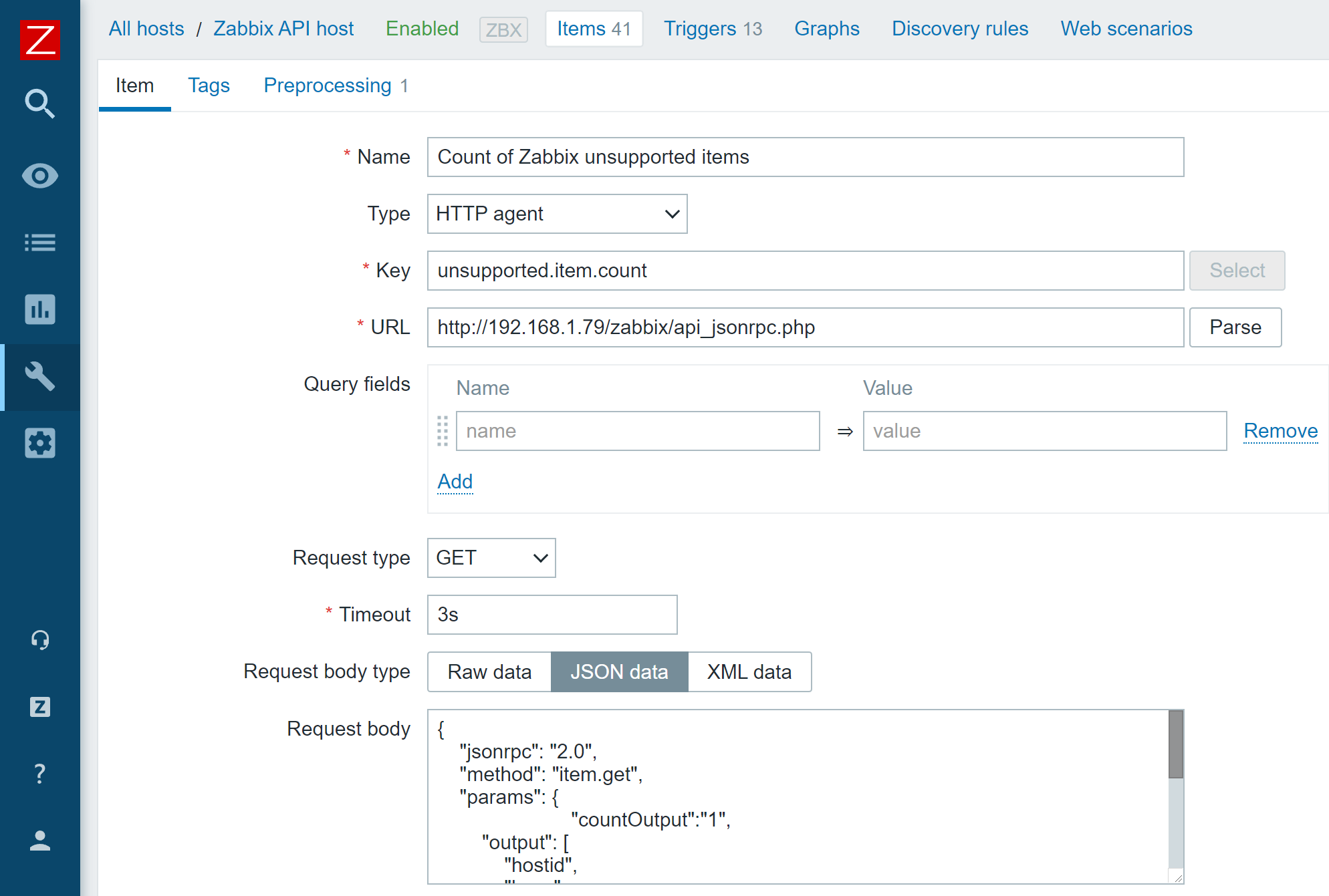
There are many different use cases where you could implement Zabbix API calls to collect some additional information. For this blog post, I will create an HTTP item that uses item.get API call to monitor the number of unsupported items.

To achieve that, I will create an HTTP item on a host (This can be the default Zabbix server host or a host dedicated to collecting metrics via Zabbix API calls) and provide the API call in the request body. Since the named API token now provides a static authentication token until it expires, I can simply use it in my API call without the need to constantly keep it updated.

An HTTP agent item that uses a Zabbix API call in its request body

{
    "jsonrpc": "2.0",
    "method": "item.get",
    "params": {
			"countOutput":"1",
			 "filter": {
 "state": "1"
 }
    },
    "id": 2,
    "auth": "b72be8cf163438aacc5afa40a112155e307c3548ae63bd97b87ff4e98b1f7657"
}

HTTP item request body, which returns a count of unsupported items

I will also use regular expression preprocessing to obtain the numeric value from the API call result – otherwise, we won’t be able to graph our value or calculate trends for it.

Regular expression preprocessing step to obtain a numeric value from our Zabbix API call result

Utilizing Zabbix API scripts in Actions

In one of our previous blog posts, we covered resolving problems automatically with the event.acknowledge API method. The logic defined in the blog post was quite complex since we needed to keep an eye out for the authentication tokens and use a custom script to keep them up to date. With named Zabbix API tokens, this use case is a lot more simple.

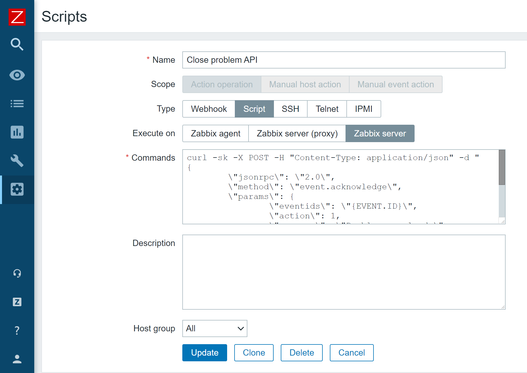
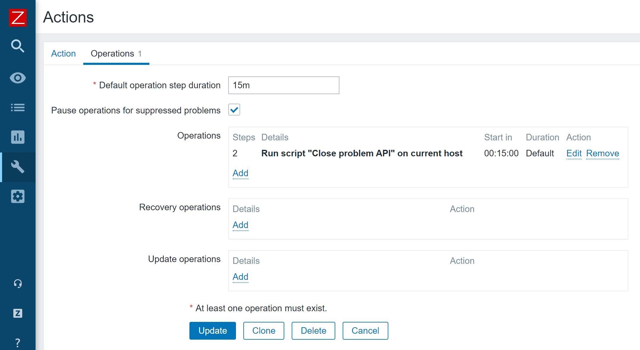
All I have to do is create an Action operation script containing my API call and pass it to an action operation.

Action operation script that invokes Zabbix event.acknowledge API method

curl -sk -X POST -H "Content-Type: application/json" -d "
{
\"jsonrpc\": \"2.0\",
\"method\": \"event.acknowledge\",
\"params\": {
\"eventids\": \"{EVENT.ID}\",
\"action\": 1,
\"message\": \"Problem resolved.\"
},
\"auth\": \"<Place your authentication token here>",
\"id\": 2
}" <Place your Zabbix API endpoint URL here>

Problem remediation script example

Now my problems will get closed automatically after the time period which I have defined in my action.

Action operation which runs our event.acknowledge Zabbix API script

These are but a few examples that we can now achieve by using API tokens. A lot of information can be obtained and filtered in a unique way via Zabbix API, thus providing you with a granular analysis of your monitored environment. If you have recently upgraded to Zabbix 5.4 or plan to upgrade to Zabbix 6.0 LTS in the future, I would recommend implementing named Zabbix API tokens to simplify your day-to-day workflow and consider the possibilities that this new feature opens up for you.

If you have any questions or if you wish to share your particular use case for data collection or task automation with Zabbix API – feel free to share them in the comments section below!

Time to Act: Bridging the Gap in Cloud Automation Adoption

Post Syndicated from Erica Azad original https://blog.rapid7.com/2021/11/11/time-to-act-bridging-the-gap-in-cloud-automation-adoption/

Time to Act: Bridging the Gap in Cloud Automation Adoption

Ready or not, the cloud is here. Across the board, an overwhelming majority of organizations recognize the value of the cloud. According to a recent survey conducted by Rapid7, 90% of respondents believe that cloud operations are critical to the competitiveness of their business. Analysts agree — Gartner recently forecasted that by 2026, cloud end-user spending will make up to 45% of overall IT spend.

We’ve established that the industry accepts the shift toward the cloud, so today we’re taking that a step further, specifically looking at attitudes toward automation in cloud security. To set the scene, 86% of respondents to our recent survey say they trust automation in their cloud security at least as much as manual effort by humans. Yet less than half (47%) have actually implemented automation in their cloud security program.

So what gives? Why does this gap exist between trust and actual adoption?

Attitudes toward automation

There’s a variety of factors that impact trust in automation, such as vendor relationships and breach history. For example, when surveying organizations about their trust in automation versus skilled professionals, 18% of those that reported a breach said they don’t trust automation. If you compare this to organizations that did not report a breach, only 14% stated they don’t trust automation. This slight uptick shows that organizations who already suffered a security incident are slightly more gun-shy of implementing automated security solutions as compared to those who didn’t.

Luckily for organizations hesitant to trust automation in the cloud, it is not an all-or-nothing exercise. There are different actions and levels of automation that can be experimented with until greater trust is achieved. For example, organizations can start with a cloud security solution automatically performing only one of monitoring, reporting, or remediation.

However, if you’re looking to benchmark against what other leading companies are doing, 56% of respondents trust automation in their cloud security program to do all three of the above — monitoring, reporting, and remediation.

Looking ahead

This growing level of trust in cloud security automation is reflected in many companies’ future plans as well. Another 25% of organizations are planning on implementing automation into their cloud security program over the next 12 months. Implementation may be lagging behind, but it’s still a goal many organizations are striving for. It’s clear that while trust must continue to be earned, the time is now for automation adoption in order to drive cloud security forward.

If you’re interested in exploring the topic of belief, trust, and reliance on automation, we recommend checking out our new report, Trust in the Cloud. This report covers many data points and survey responses, diving into the gap between automation attitudes and implementation.

Security updates for Thursday

Post Syndicated from original https://lwn.net/Articles/875813/rss

Security updates have been issued by Debian (icinga2, libxstream-java, ruby-kaminari, and salt), Fedora (awscli, cacti, cacti-spine, python-boto3, python-botocore, radeontop, and rust), Mageia (firefox, libesmtp, libzapojit, sssd, and thunderbird), openSUSE (samba and samba and ldb), SUSE (firefox, pcre, qemu, samba, and samba and ldb), and Ubuntu (firejail, linux-bluefield, linux-gke-5.4, linux-oracle, linux-oracle-5.4, linux-oem-5.10, linux-oem-5.14, and python-py).

Handy Tips #11: Collect and send custom metrics with Zabbix sender

Post Syndicated from vitalijsm original https://blog.zabbix.com/handy-tips-11-collect-and-send-custom-metrics-with-zabbix-sender/17452/

Collect custom metrics from your in-house applications and forward them to your Zabbix instance by utilizing the Zabbix sender command-line tool.

As you scale up our monitoring, you will inevitably encounter a situation where a particular metric can be quite complex to collect with native monitoring techniques.

(more…)

По телевизора

Post Syndicated from original http://dni.li/2021/11/11/broadcast/

Гледала съм Broadcast News преди много години. Харесала го бях. Определила го бях за умно-забавен по един тъжен начин, сатиричен и истински, примиренчески малко, уви, но непресторен. Спомням си сюжета, но подробностите малко ми се губят по разбираеми причини.

Това, което помня съвсем ясно обаче, е как (посредственият) Том учеше (умния, добре информиран, но смачкан) Арън да се държи пред камерата. Дръпна сакото му назад, накара го да опъне рамена и изведнъж от кюфте Арън се превърна в съвсем приемлив на външен вид мъж. Рейтингът му се вдигна и почти успя да се задържи на работа в телевизията (ама се провали от притеснение накрая, де).

Та… няма ли някой Том в тази България, който да обясни на кандидатите за депутати и президенти, че трябва да си мият косата редовно, да си гладят дрехите, да не стоят приведени и отпуснати, нито пък да менспредват все едно са се пльоснали на дивана у дома? На ей такива елементарни неща да ги светне.

Няма май.

Measure and Improve Your Application Resilience with AWS Resilience Hub

Post Syndicated from Sébastien Stormacq original https://aws.amazon.com/blogs/aws/monitor-and-improve-your-application-resiliency-with-resilience-hub/

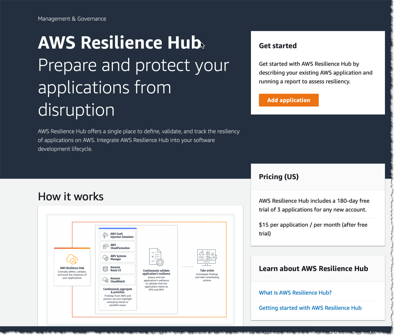
I am excited to announce the immediate availability of AWS Resilience Hub, a new AWS service designed to help you define, track, and manage the resilience of your applications.

You are building and managing resilient applications to serve your customers. Building distributed systems is hard; maintaining them in an operational state is even harder. The question is not if a system will fail, but when it will, and you want to be prepared for that.

Resilience targets are typically measured by two metrics: Recovery Time Objective (RTO), the time it takes to recover from a failure, and Recovery Point Objective (RPO), the maximum window of time in which data might be lost after an incident. Depending on your business and application, these can be measured in seconds, minutes, hours, or days.

AWS Resilience Hub lets you define your RTO and RPO objectives for each of your applications. Then it assesses your application’s configuration to ensure it meets your requirements. It provides actionable recommendations and a resilience score to help you track your application’s resiliency progress over time. Resilience Hub gives a customizable single dashboard experience, accessible through the AWS Management Console, to run assessments, execute prebuilt tests, and configure alarms to identify issues and alert the operators.

AWS Resilience Hub discovers applications deployed by AWS CloudFormation (this includes SAM and CDK applications), including cross Regions and cross account stacks. Resilience Hub also discovers applications from Resource Groups and tags or chooses from applications already defined in AWS Service Catalog AppRegistry.

The term “application” here refers not just to your application software or code; it refers to the entire infrastructure stack to host the application: networking, virtual machines, databases, and so on.

Resilience assessment and recommendations
AWS Resilience Hub’s resilience assessment utilizes best practices from the AWS Well-Architected Framework to analyze the components of your application and uncover potential resilience weaknesses caused by incomplete infrastructure setup, misconfigurations, or opportunities for additional configuration improvements. Resilience Hub provides actionable recommendations to improve the application’s resilience.

For example, Resilience Hub validates that the application’s Amazon Relational Database Service (RDS), Amazon Elastic Block Store (EBS), and Amazon Elastic File System (Amazon EFS) backup schedule is sufficient to meet the application’s RPO and RTO you defined in your resilience policy. When insufficient, it recommends improvements to meet your RPO and RTO objectives.

The resilience assessment generates code snippets that help you create recovery procedures as AWS Systems Manager documents for your applications, referred to as standard operating procedures (SOPs). In addition, Resilience Hub generates a list of recommended Amazon CloudWatch monitors and alarms to help you quickly identify any change to the application’s resilience posture once deployed.

Continuous resilience validation
After the application and SOPs have been updated to incorporate recommendations from the resilience assessment, you may use Resilience Hub to test and verify that your application meets its resilience targets before it is released into production. Resilience Hub is integrated with AWS Fault Injection Simulator (FIS), a fully managed service for running fault injection experiments on AWS. FIS provides fault injection simulations of real-world failures, such as network errors or having too many open connections to a database. Resilience Hub also provides APIs for development teams to integrate their resilience assessment and testing into their CI/CD pipelines for ongoing resilience validation. Integrating resilience validation into CI/CD pipelines helps ensure that every change to the application’s underlying infrastructure does not compromise its resilience.

Visibility
AWS Resilience Hub provides a comprehensive view of your overall application portfolio resilience status
through its dashboard. To help you track the resilience of applications, Resilience Hub aggregates and
organizes resilience events (for example, unavailable database or failed resilience validation), alerts, and insights from services like Amazon CloudWatch and AWS Fault Injection Simulator (FIS). Resilience Hub also generates a resilience score, a scale that indicates the level of implementation for recommended resilience tests, alarms and recovery SOPs. This score can be used to measure resilience improvements over time.

The intuitive dashboard sends alerts for issues, recommends remediation steps, and provides a single place to manage application resilience. For example, when a CloudWatch alarm triggers, Resilience Hub alerts you and recommends recovery procedures to deploy.

AWS Resilience Hub in Action
I developed a non-resilient application made of a single EC2 instance and an RDS database. I’d like Resilience Hub to assess this application. The CDK script to deploy this application on your AWS Account is available on my GitHub repository. Just install CDK v2 (npm install -g aws-cdk@next) and deploy the stack (cdk bootstrap && cdk deploy --all).

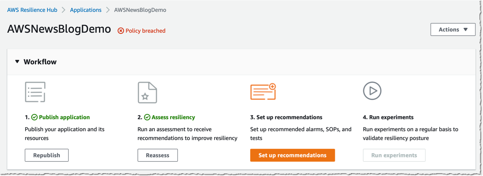
There are four steps when using Resilience Hub:

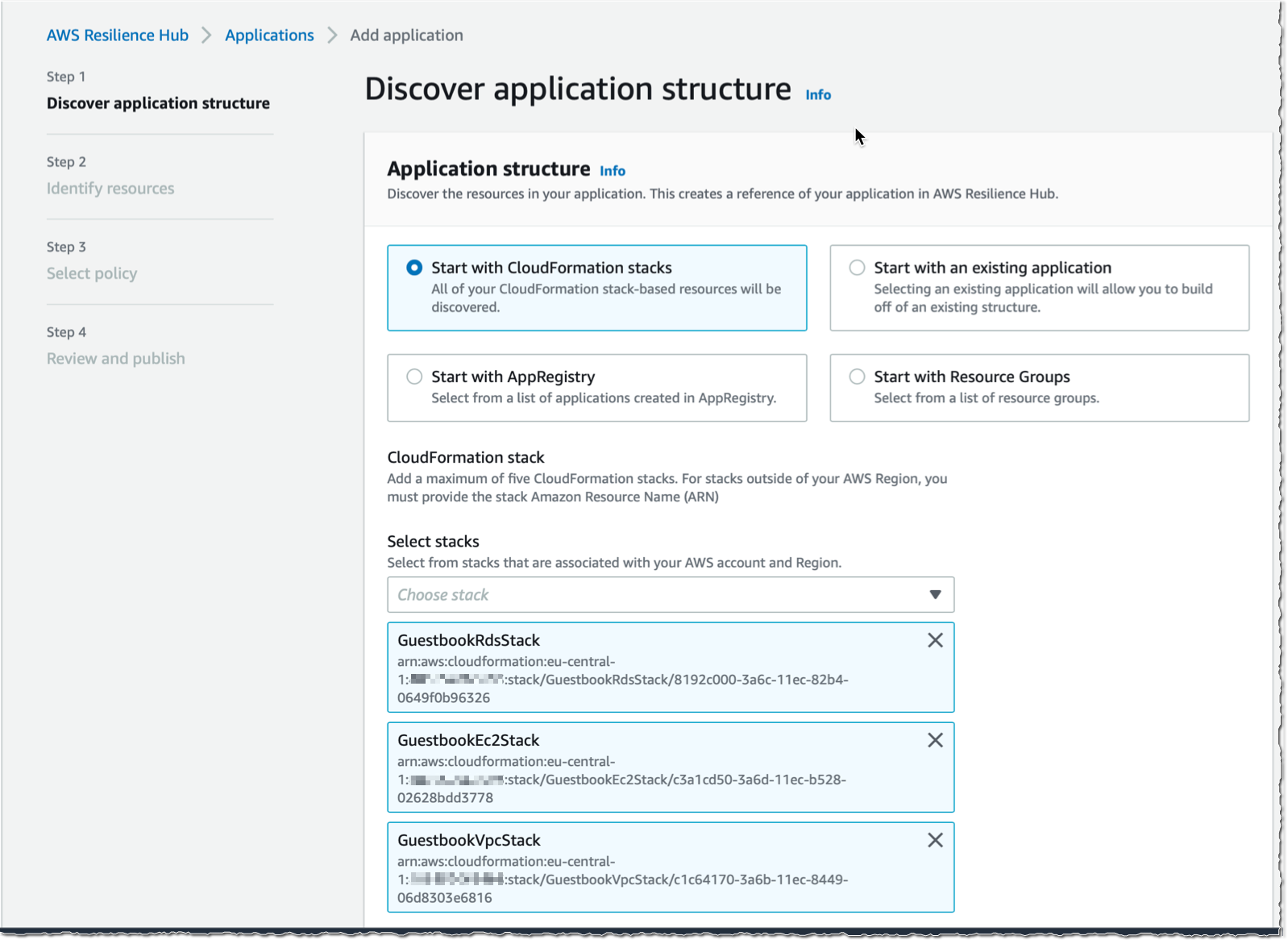
  • I first add the application to assess. I can start with CloudFormation stacks, AppRegistry, Resource Groups, or another existing application.
  • Second, I define my resilience policy. The policy document describes my RTO and RPO objectives for incidents that might impact either my application, my infrastructure, an entire availability zone, or an entire AWS Region.
  • Third, I run an assessment against my application. The assessment lists policy breaches, if any, and provides a set of recommendations, such as creating CloudWatch alarms, standard operating procedures documents, or fault injection experiment templates.
  • Finally, I might setup any of the recommendations made or run experiments on a regular basis to validate the application’s resilience posture.

Preparation
To start, I open my browser and navigate to the AWS Management Console. I select AWS Resilience Hub and select Add application.

Resilience hub add application

My sample app is deployed with three CloudFormation stacks: a network, a database, and an EC2 instance.  I select these three stacks and select Next on the bottom of the screen:

Resilience Hub add cloud formations tack

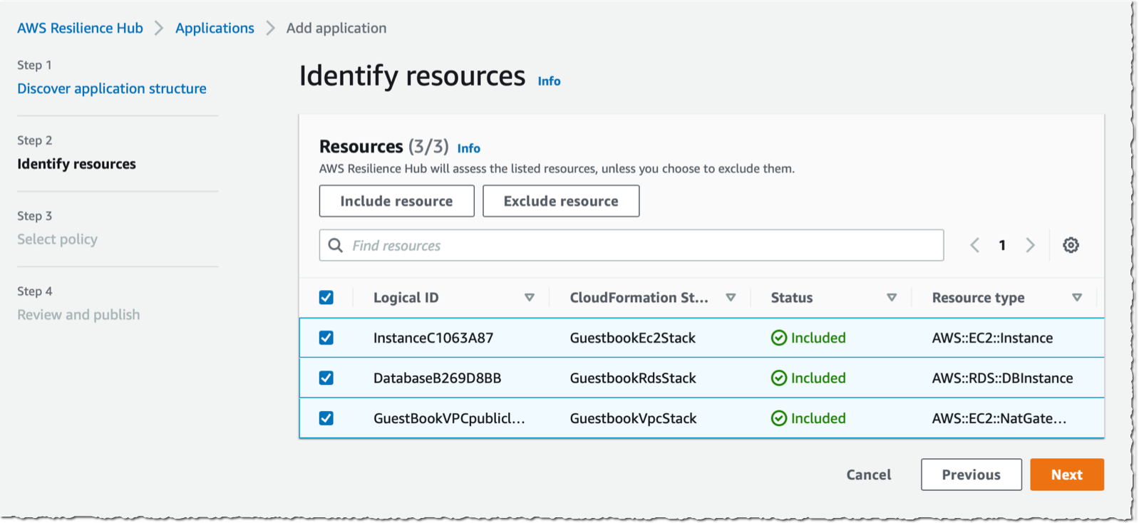
Resilience Hub detects the resources created by these stacks that might affect the resilience of my applications and I select the ones I want to include or exclude from the assessments and click Next. In this example, I select the NAT gateway, the database instance, and the EC2 instance.

Resilience Hub Select resources

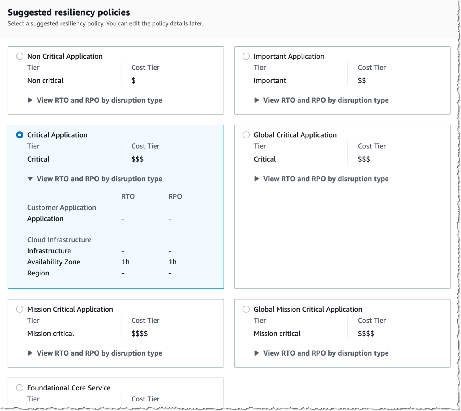
I create a resilience policy and associate it with this application. I can choose from policy templates or create a policy from scratch. A policy includes a name and the RTO and RPO values for four types of incidents: the ones affecting my application itself, like a deployment error or a bug at code level; the ones affecting my application infrastructure, like a crash of the EC2 instance; the ones affecting an availability zone; and the ones affecting an entire region. The values are expressed in seconds, minutes,  hours, or days.

Resilience Hub Create Policy

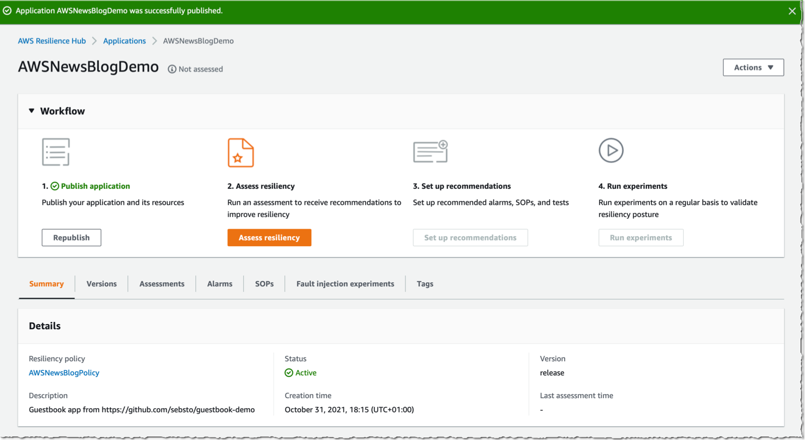
Finally, I review my choices and select Publish.

Assessment
Once this application and its policy are published, I start the assessment by selecting Assess resiliency.

Resilience Hub Assess resiliency

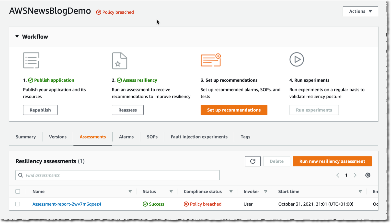
Without surprise, Resilience Hub reports my resilience policy is breached.

Resilience Hub Policy breach

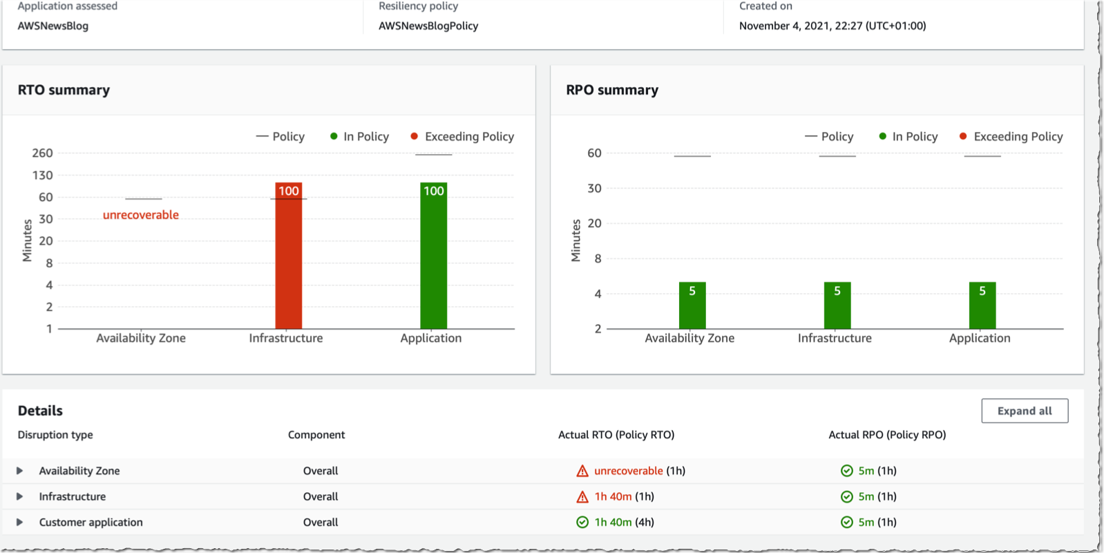
I select the report to get the details.  The dashboard shows how Region, availability zone, infrastructure and application-level incident expected RTO/RPO compare to my policy.

Resilience Hub Assessment dashboard

I have access to Resiliency recommendations and Operational recommendations.

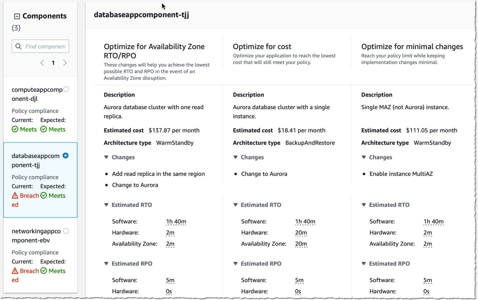
In Resiliency recommendations, I see if components of my application are compliant with the resilience policy. I also discover recommendations to Optimize for availability zone RTO/RPO, Optimize for cost, or Optimize for minimal changes.

Resilience Hub Optimisation

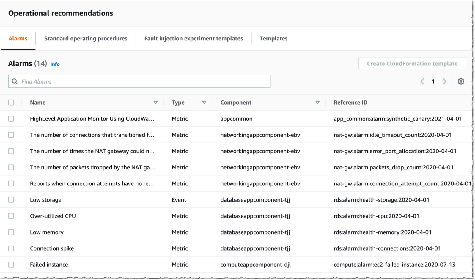
In Operational recommendations, on the first tab, I see a list of proposed Alarms to create in CloudWatch.

Resilience Hub Alarms

The second tab lists recommended Standard operating procedures. These are Systems Manager documents I can run on my infrastructure, such as Restore from Backup.

Resilience Hub SOP

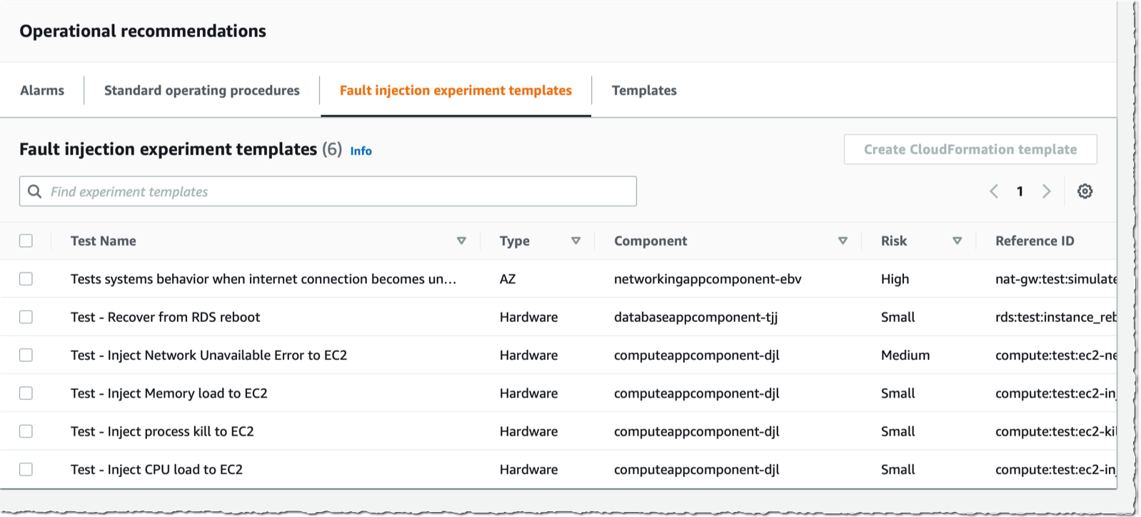
The third tab (Fault injection experiment templates) proposes experiments to run on my infrastructure to test its resilience. Experiments are run with FIS. Proposed experiments are Inject memory load or Inject process kill.

Resilience Hub - FIS

When I select Set up recommendations, Resilience Hub generates CloudFormation templates to create the alarms or to execute the SOP or experiment proposed.

Resilience Hub - Set up recommandations

The follow up screens are quite self-explanatory. Once generated, templates are available to execute in the Templates tab. I apply the template and observe how it impacts the resilience score of the application.

Resilience Hub Resilience score

The CDK script you used to deploy the sample applications also creates a highly available infrastructure for the same application. It has a load balancer, an auto scaling group, and a database cluster with two nodes. As an exercise, run the same assessment report on this application stack and compare the results.

Pricing and Availability
AWS Resilience Hub is available today in US East (Ohio), US East (N. Virginia), US West (Oregon), Asia Pacific (Singapore), Asia Pacific (Tokyo), Europe (Ireland), and Europe (Frankfurt). We will add more regions in the future.

As usual, you pay only for what you use. There are no upfront costs or minimum fees. You are charged based on the number of applications you described in Resilience Hub. You can try Resilience Hub free for 6 months, up to 3 applications. After that, Resilience Hub‘s price is $15.00 per application per month. Metering begins once you run the first resilience assessment in Resilience Hub. Remember that Resilience Hub might provision services for you, such as CloudWatch alarms, so additional charges might apply. Visit the pricing page to get the details.

Let us know your feedback and build your first resilience dashboard today.

— seb

Query data in Amazon OpenSearch Service using SQL from Amazon Athena

Post Syndicated from Behram Irani original https://aws.amazon.com/blogs/big-data/query-data-in-amazon-opensearch-service-using-sql-from-amazon-athena/

Amazon Athena is an interactive serverless query service to query data from Amazon Simple Storage Service (Amazon S3) in standard SQL. Amazon OpenSearch Service (successor to Amazon Elasticsearch Service) is a fully managed, open-source, distributed search and analytics suite derived from Elasticsearch, allowing you to run OpenSearch Service or Elasticsearch clusters at scale without having to manage hardware provisioning, software installation, patching, backups, and so on.

Although both services have their own use cases, there might be situations when you want to run queries that combine data in Amazon S3 with data in an Amazon OpenSearch Service Cluster. In such cases, federated queries in Athena are a good option—they provide the capability to combine data from multiple data sources and analyze them in a single query. The federated query feature works by using data source connectors that are built for different data sources. To allow Amazon OpenSearch Service to be one of the sources that Athena can query against, AWS has made available a data source connector for OpenSearch Service clusters to be queried from Athena.

This post demonstrates how to query data in Amazon OpenSearch Service and Amazon S3 in a single query. We use the data made available in the public COVID-19 data lake, documented as part of the post A public data lake for analysis of COVID-19 data.

In particular, we use the following two datasets:

  1. alleninstitute_metadata : Metadata on papers pulled from the COVID-19 Open Research Dataset (CORD-19). The sha column indicates the paper ID, which is the file name of the paper in the data lake. This dataset is stored in Amazon OpenSearch Service because it contains the column abstract, which you can search on.
  2. alleninstitute_comprehend_medical : Results containing annotations obtained by running the papers in the preceding dataset through Amazon Comprehend Medical. This is accessed from its public storage at s3://covid19-lake/alleninstitute/CORD19/comprehendmedical/comprehend_medical.json.

Data flow when combining data from Amazon OpenSearch Service and Amazon S3

The data source connectors are implemented as AWS Lambda functions. When a user issues a query that combines data from Amazon OpenSearch Service and Amazon S3, Athena refers to the AWS Glue Data Catalog metadata to look up the table definitions. For the table whose data is in Amazon S3, Athena fetches the data from Amazon S3. For the tables that are in Amazon OpenSearch Service, Athena invokes the Lambda function (part of the data source connector application) to read the data from Amazon OpenSearch Service. Depending on the amount of data, you can invoke this function multiple times in parallel for the same query to enable faster reads.

The following diagram illustrates this data flow.

Set up the two data sources using AWS CloudFormation

To prepare for querying both data sources, launch the AWS CloudFormation template using the “Launch Stack” button below. All you need to do is choose Create stack.

To run the CloudFormation stack, you need to be logged in to an AWS account with permissions to do the following:

  • Create a CloudFormation stack
  • Create an Identity and Access Management (IAM) role
  • Create a Lambda function, assign an IAM role to it, and invoke it
  • Launch an OpenSearch Service cluster
  • Create AWS Glue databases and table
  • Create an S3 bucket

For instructions on creating a CloudFormation stack, see Get started.

For more information about controlling permissions and access for these services, see the following resources:

The CloudFormation template creates the following:

  • A table in the AWS Glue Data Catalog named alleninstitute_comprehend_medical that points to the S3 location s3://covid19-lake/alleninstitute/CORD19/comprehendmedical/comprehend_medical.json. This contains the results extracted from the CORD-19 data using the natural language processing service Amazon Comprehend Medical.
  • An S3 bucket with the name athena-es-connector-spill-bucket- followed by the first few characters from the stack ID to keep the bucket name unique.
  • An OpenSearch Service cluster with the name es-alleninstitute-data, which has two instances configured to allow a role to access the cluster.
  • An IAM role to access the OpenSearch Service cluster.
  • A Lambda function that contains a piece of Python code that reads all the metadata of the papers along with the abstract. This data is available as JSON at s3://covid19-lake/alleninstitute/CORD19/json/metadata/. For this post, we load just one of the four JSON files available.
  • A custom resource that invokes the Lambda function to load the data into the OpenSearch Service cluster.

The stack can take 15–30 minutes to complete.

When the stack is fully deployed, navigate to the Outputs tab of the stack and note the name of the S3 bucket created (the value for SpillBucket).

For the rest of the steps, you need permissions to do the following:

Deploy the Amazon Athena OpenSearch connector

When the OpenSearch Service domain with an index containing the metadata related to the COVID-19 research papers and the AWS Glue table pointing to the Amazon Comprehend Medical output data is ready, you can deploy the Amazon Athena OpenSearch connector using the AWS Serverless Application Repository.

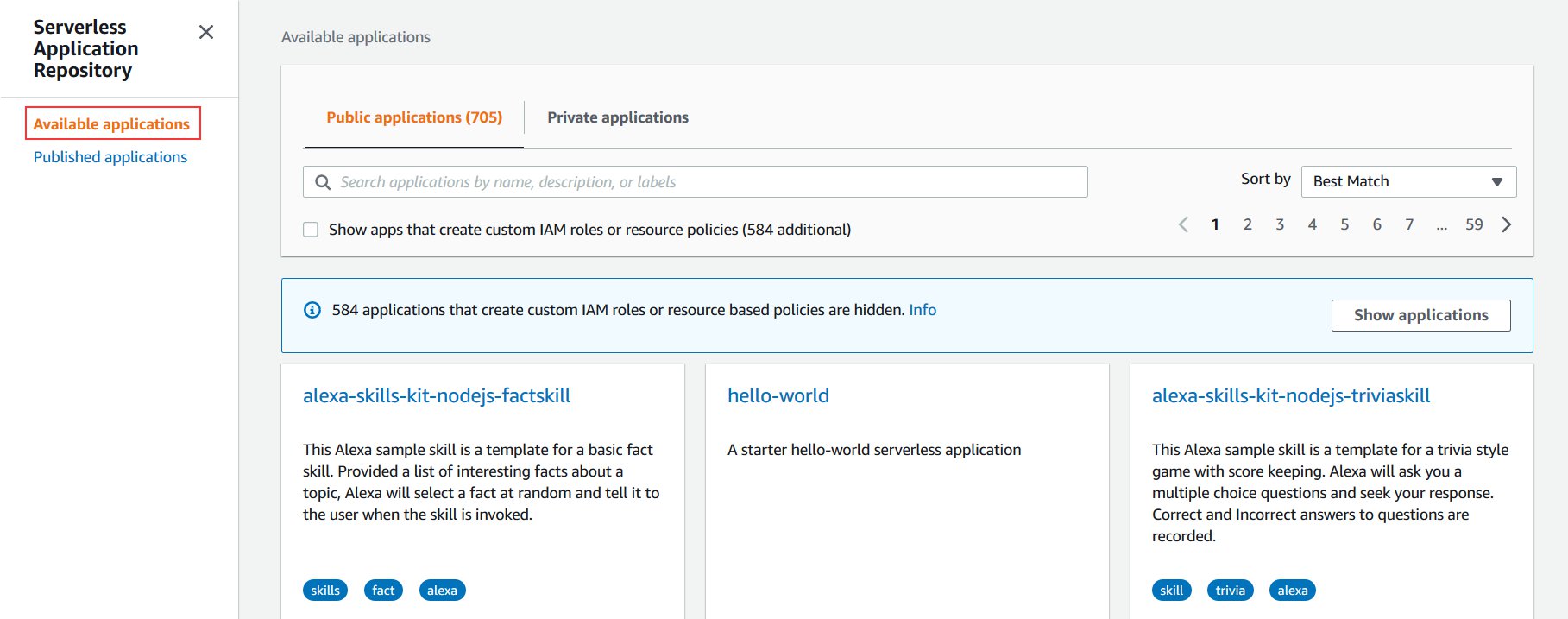
  1. On the AWS Serverless Application Repository console, choose Available applications.
  2. Search for Athena Elasticsearch and select Show apps that create custom IAM roles or resource policies.
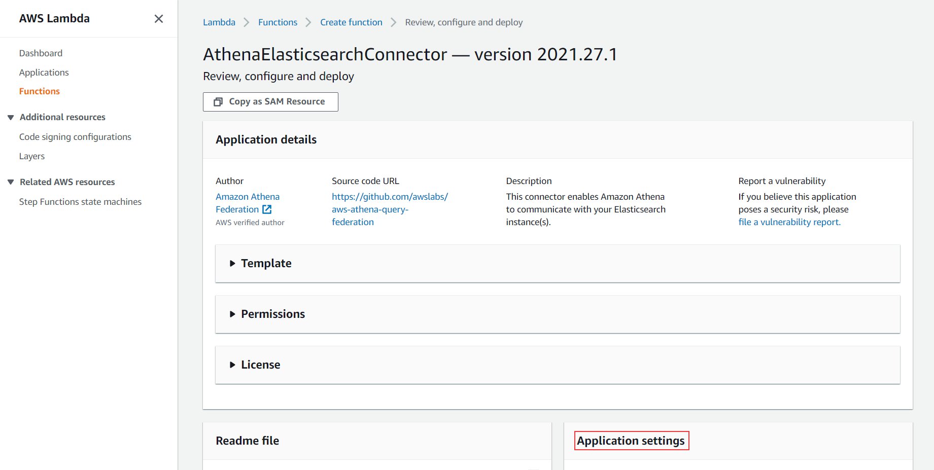
  3. Choose AthenaElasticsearchConnector.

You’re redirected to the application screen.

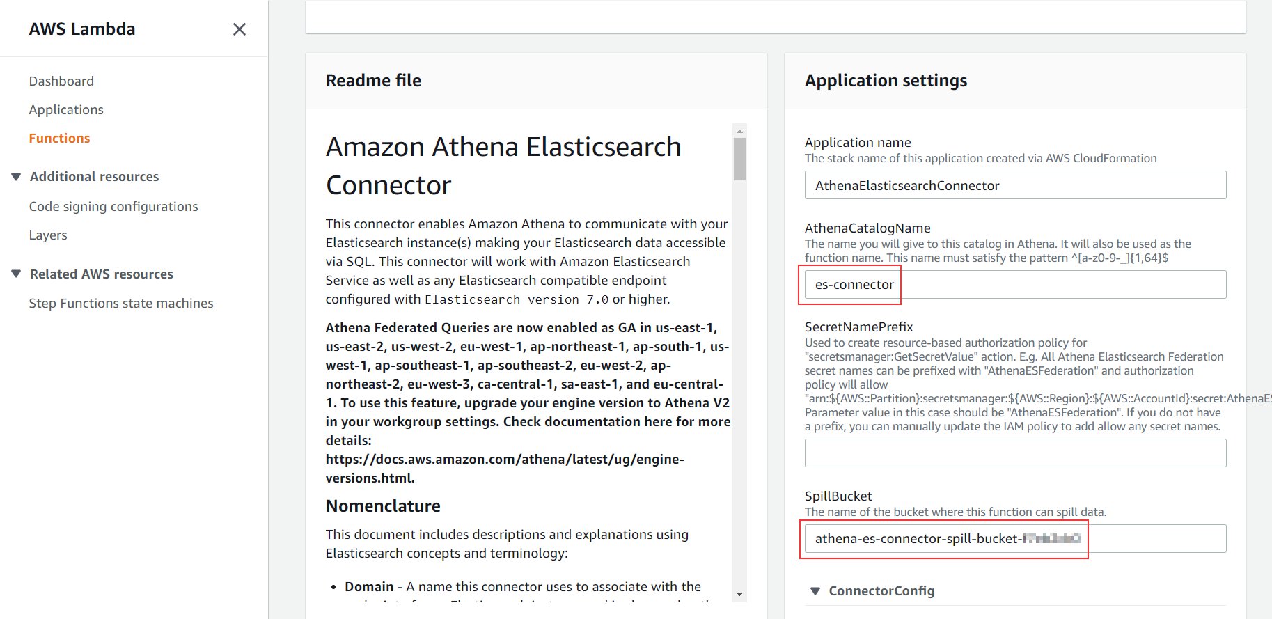
  1. Scroll down to the Application settings section.
  2. For AthenaCatalogName, enter a name (for this post, we use es-connector).

This name is the name of the application and the Lambda function that connects to Amazon OpenSearch Service every time you run a query from Athena. For more details about all the parameters, refer to the connector’s GitHub page.

  1. For SpillBucket, enter the name you noted in the previous section when we deployed the CloudFormation stack (it begins with athena-es-connector-spill-bucket).
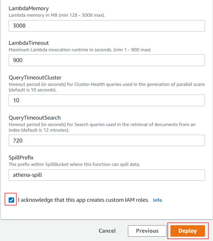
  2. Leave all other settings as default.
  3. Select I acknowledge that this app creates custom IAM roles.
  4. Choose Deploy.

In a few seconds, you’re redirected to the Applications page. You can see the status of your deployment on the Deployments tab. The deployment takes 1–2 minutes to complete.

Create a new data source in Athena

Now that the connector application has been deployed, it’s time to set up the OpenSearch Service domain to show as a catalog on Athena.

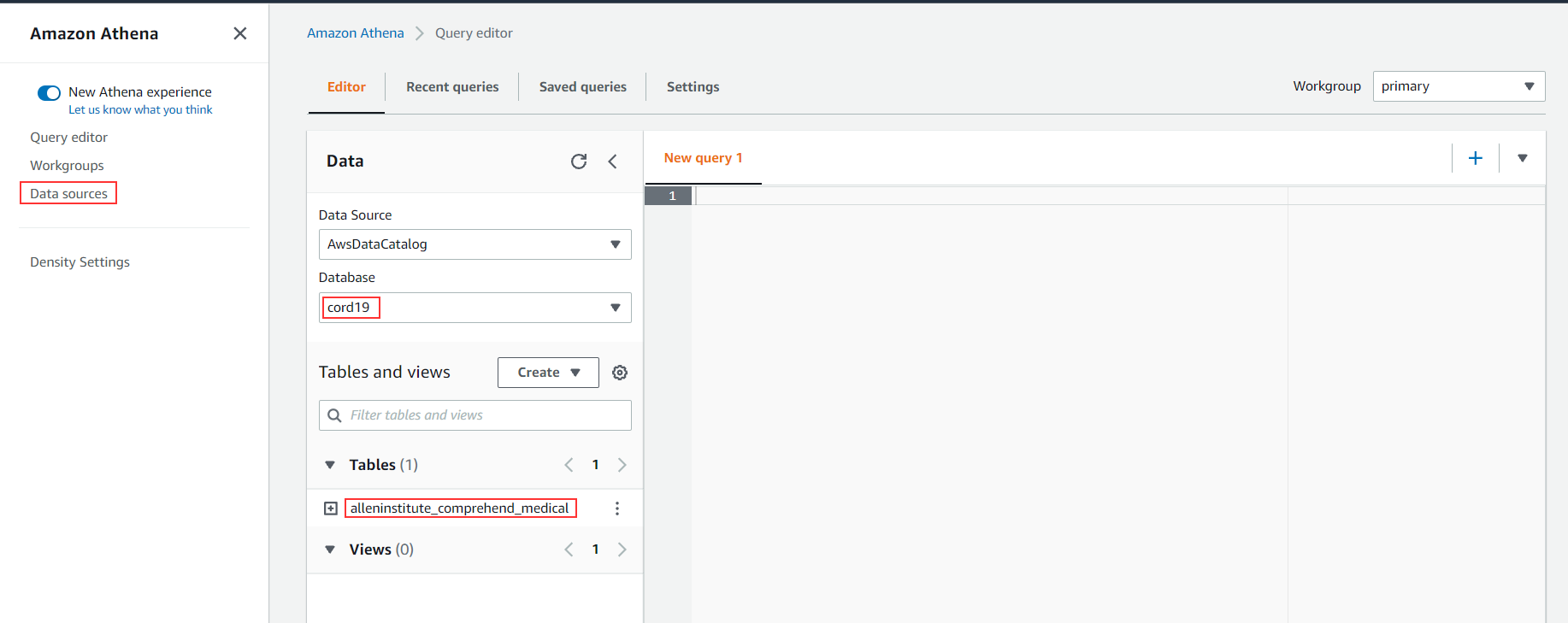
  1. On the Athena console, navigate to the cord19 database.

The database contains the table alleninstitute_comprehend_medical, which was created as part of the CloudFormation template. This refers to the data sitting in Amazon S3 at s3://covid19-lake/alleninstitute/CORD19/comprehendmedical/.

  1. Choose Data sources in the navigation pane.
  2. Choose Connect data source.
  3. Select Custom data source.
  4. For Data source name, enter a name (for example, es-cord19-catalog).
  5. Select Use an existing Lambda function and choose es-connector on the drop-down menu.
  6. Choose Connect data source.
  7. Choose Next.
  8. For Lambda function, choose es-connector.
  9. Choose Connect.

A new catalog es-cord19-catalog should now be available, as in the following screenshot.

  1. On the Query editor tab, for Data source, choose es-cord19-catalog.

You can now query this data source from Athena.

Query OpenSearch Service domains from Athena

When you choose the es-cord19-catalog data source, the Lambda function (which was part of the connector application that we deployed) gets invoked and fetches the details about the domain and the index. The OpenSearch Service domain shows up as a database, and the index is shown as a table. You can also query the table with the following query:

select count(*) from "es-cord19-catalog"."es-alleninstitute-data".alleninstitute_metadata

Now you can join data from both Amazon OpenSearch Service and Amazon S3 with queries, such as the following:

select es.title, es.url from 
"es-cord19-catalog"."es-alleninstitute-data".alleninstitute_metadata es
    inner join
AwsDataCatalog.cord19.alleninstitute_comprehend_medical s3
    on es.sha = s3.paper_id
WHERE 
    array_join(s3.dx_name, ',') like '%infectious disease%'

The preceding query gets the title and the URL of all the research papers where the diagnosis was related to infectious diseases.

The following screenshot shows the query results.

Clean up

To clean up the resources created as part of this post, complete the following steps:

  1. On the Amazon S3 console, locate and select your S3 bucket (the same bucket you noted from the CloudFormation stack).
  2. Choose Empty.

You can also achieve this by running the following command from a command line:

aws s3 rm s3://athena-es-connector-spill-bucket-f7eb2cb0 –recursive
  1. On the AWS CloudFormation console, delete the stack you created.
  2. Delete the stack created for the Amazon Athena OpenSearch connector application. The default name is serverlessrepo-AthenaElasticsearchConnector.
  3. On the Athena console, delete the es-cord19-catalog data source.

You can also delete the data source with the following command:

aws athena delete-data-catalog --name "es-cord19-catalog"

Conclusion

In this post, we saw how to combine data from OpenSearch Service clusters with other data sources like Amazon S3 to run federated queries. You can apply this solution to other use cases, such as combining AWS CloudTrail logs loaded into OpenSearch Service clusters with VPC flow logs data in Amazon S3 to analyze unusual network traffic, or combining product reviews data in Amazon OpenSearch Service with product data in Amazon S3 or other data sources. You can also pull data from Amazon OpenSearch Service and create an AWS Glue table out of it using a CTAS query in Athena.

To learn more about the Amazon Athena OpenSearch connector and its other configuration options, see the GitHub repo.

To learn more about query federation in Athena, refer to Using Amazon Athena Federated Query or Query any data source with Amazon Athena’s new federated query.


About the Authors

Behram Irani, Sr Analytics Solutions Architect

Madhav Vishnubhatta, Sr Technical Account Manager

Update to GLBA Security Requirements for Financial Institutions

Post Syndicated from Harley Geiger original https://blog.rapid7.com/2021/11/10/update-to-glba-security-requirements-for-financial-institutions/

Update to GLBA Security Requirements for Financial Institutions

Heads up financial institutions: the Federal Trade Commission (FTC) announced the first cybersecurity updates to the Gramm Leach-Bliley Act (GLBA) Safeguards Rule since 2003. The new rule strengthens the required security safeguards for customer information. This includes formal risk assessments, access controls, regular penetration testing and vulnerability scanning, and incident response capabilities, among other things.

Several of these changes go into effect in November 2022, to provide organizations time to prepare for compliance. Below, we’ll detail the changes in comparison to the previous rule.

Background on the Safeguards Rule

GLBA requires, among other things, a wide range of “financial institutions” to protect customer information. Enforcement for GLBA is split up among several different federal agencies, with FTC jurisdiction covering non-banking financial institutions in the Safeguards Rule. Previously, the Safeguards Rule left the implementation details of several aspects of the information security program up to the financial institution, based on its risk assessment.

The Safeguards Rule broad definition of “financial institutions” includes non-bank businesses that offer financial products or services — such as retailers, automobile dealers, mortgage brokers, non-bank lenders, property appraisers, tax preparers, and others. The definition of “customer information” is also broad, to include any record containing non-public personally identifiable information about a customer that is handled or maintained by or on behalf of a financial institution.

Updates to the Safeguards Rule

Many of the other updates concern strengthened requirements on how financial institutions must implement aspects of their security programs. Below is a short summary of changes. Where applicable, we include citations to both the updated rule (starting at page 123) and the previous rule (at 16 USC 314) for easy comparison.

Overall security program

  • Current rule: Financial institutions must maintain a comprehensive, written information security program with administrative, technical, and physical safeguards to ensure the security, confidentiality, and integrity of customer information. 16 USC 314.3(a)-(b).
  • Updated rule: The updated rule now requires the information security program to include the processes and safeguards listed below (i.e., risk assessment, security safeguards, etc.). 16 USC 314.3(a).
  • Approx. effective date: November 2022

Risk assessment

  • Current rule: Financial institutions are required to identify internal and external risks to security, confidentiality, and integrity of customer information. The risk assessment must include employee training, risks to information systems, and detecting and responding to security incidents and events. 16 USC 314.4(b).
  • Updated rule: The update includes more specific criteria for what the risk assessment must include. This includes criteria for evaluating and categorizing of security risks and threats, and criteria for assessing the adequacy of security safeguards. The risk assessment must describe how identified risks will be mitigated or accepted. The risk assessment must be in writing. 16 USC 314.4(b).
  • Approx. effective date: November 2022

Security safeguards

  • Current rule: Financial institutions must implement safeguards to control the risks identified through the risk assessment. 16 USC 314.4(c). Financial institutions must require service providers to maintain safeguards to protect customer information. 16 USC 314.4(d).
  • Updated rule: The updated rule requires that the safeguards must include
    – Access controls, including providing the least privilege;
    – Inventory and classification of data, devices, and systems;
    – Encryption of customer information at rest and in transit over internal networks;
    – Secure development practices for in-house software and applications;
    – Multi-factor authentication;
    – Secure data disposal;
    – Change management procedures; and
    – Monitoring activity of unauthorized users and detecting unauthorized access or use of customer information. 16 USC 314.4(c)(1)-(8).
  • Approx. effective date: November 2022

Testing and evaluation

  • Current rule: Financial institutions must regularly test or monitor the effectiveness of the security safeguards, and make adjustments based on the testing. 16 USC 314.4(c), (e).
  • Updated rule: Regular testing of safeguards must now include either continuous monitoring or periodic penetration testing (annually) and vulnerability assessments (semi-annually). 16 USC 314.4(d).
  • Approx. effective date: November 2022

Incident response

  • Current rule: Financial institutions must include cybersecurity incident detection and response in their risk assessments, and have safeguards to address those risks. 16 USC 314.4(b)(3)-(c).
  • Updated rule: Financial institutions are required to establish a written plan for responding to any security event materially affecting confidentiality, integrity, or availability of customer information. 16 USC 314.4(h).
  • Approx. effective date: November 2022

Workforce and personnel

  • Current rule: Financial institutions must designate an employee to coordinate the information security program. 16 USC 314.4(a). Financial institutions must select service providers that can maintain security and require service providers to implement the safeguards. 16 USC 314.4(d).
  • Updated rule: The rule now requires designation of a single “qualified individual” to be responsible for the security program. This can be a third-party contractor. 16 USC 314.4(a). Financial institutions must now provide security awareness training and updates to personnel. 16 USC 314.4(e). The rule now also requires periodic reports to a Board of Directors or governing body regarding all material matters related to the information security program. 16 USC 314.4(i).
  • Approx. effective date: November 2022

Scope of coverage

  • Updated rule: The FTC update expands on the definition of “financial institution” to require “finders” — companies that bring together buyers and sellers — to follow the Safeguards Rule. 16 USC 314.2(h)(1). However, financial institutions that maintain information on fewer than 5,000 consumers are exempt from the requirements of a written risk assessment, continuous monitoring or periodic pentesting and/or vulnerability scans, incident response plan, and annual reporting to the Board. 16 USC 314.6.
  • Approx. effective date: November 2021 (unlike many of the other updates, this item is not delayed for a year)

Incident reporting next?

In addition to the above, the FTC is also considering requirements that financial institutions report cybersecurity incidents and events to the FTC. Similar requirements are in place under the Cybersecurity Regulation at the New York Department of Financial Services. If the FTC moves forward with these incident reporting requirements, financial institutions could expect the requirements to be implemented later in 2022 or early 2023.

Financial institutions with robust security programs will already be performing many of these practices. For them, the updated Safeguards Rule will not represent a sea change in internal security operations. However, by making these security practices a formal regulatory requirement, the updated Safeguards will make accountability and compliance even more important.

NEVER MISS A BLOG

Get the latest stories, expertise, and news about security today.

[Security Nation] Michael Powell on Being a Cyber Envoy

Post Syndicated from Rapid7 original https://blog.rapid7.com/2021/11/10/security-nation-michael-powell-on-being-a-cyber-envoy/

[Security Nation] Michael Powell on Being a Cyber Envoy

In this episode of Security Nation, Jen and Tod chat with Michael Powell about his work as specialist cyber representative to North America for the UK’s Department for International Trade (DIT). After confirming that Michael is not actually a spy (or is he?), they discuss the excitement and challenges of creating cross-continental collaboration on some of the most pressing cybersecurity issues organizations face today — including supply chain risk, ransomware, and the role of government in moving the needle on these threats.

Stick around for our Rapid Rundown, where Tod and Jen talk about inTheWild, a new open-source, community-driven database for vulnerabilities that are being actively exploited.

Michael Powell

[Security Nation] Michael Powell on Being a Cyber Envoy

Michael Powell is DIT’s cyber sector trade specialist in North America. His background includes over 15 years of experience with major enterprise and start-ups, defining and delivering managed and professional cybersecurity services for law enforcement and commercial organizations. Michael is based on the East Coast, advising UK companies on North America market entry – leveraging DIT’s network to discuss resourcing, legislation, and the evolving needs of buyers. He is a proponent of workforce diversity across the tech sector and has a strong technical background to understand and discuss solutions to complex organizational cybersecurity problems. When not advising UK companies, he works closely with the London specialist teams, and partners, on investment opportunities and being an in-market voice for the UK cybersecurity ecosystem.

Show notes

Interview links

Rapid Rundown links

Like the show? Want to keep Jen and Tod in the podcasting business? Feel free to rate and review with your favorite podcast purveyor, like Apple Podcasts.

Want More Inspiring Stories From the Security Community?

Subscribe to Security Nation Today

AWS achieves GSMA Security Certification for Europe (Paris) Region

Post Syndicated from Janice Leung original https://aws.amazon.com/blogs/security/aws-achieves-gsma-security-certification-for-europe-paris-region/

We continue to expand the scope of our assurance programs at Amazon Web Services (AWS) and are pleased to announce that our Europe (Paris) Region is now certified by the GSM Association (GSMA) under its Security Accreditation Scheme Subscription Management (SAS-SM) with scope Data Center Operations and Management (DCOM). This is an addition to our US East (Ohio) Region, which received certification in September 2021. This alignment with GSMA requirements demonstrates our continuous commitment to adhere to the heightened expectations for cloud service providers. AWS customers who provide embedded Universal Integrated Circuit Card (eUICC) for mobile devices can run their remote provisioning applications with confidence in the AWS Cloud in the GSMA-certified Regions.

As of this writing, 72 services offered in the Europe (Paris) Region and 128 services offered in the US East (Ohio) Region are in scope of this certification. For up-to-date information, including when additional services are added, see the AWS Services in Scope by Compliance Program and choose GSMA.

AWS was evaluated by independent third-party auditors chosen by GSMA. The Certificate of Compliance that shows that AWS achieved GSMA compliance status is available on the GSMA Website and through AWS Artifact. AWS Artifact is a self-service portal for on-demand access to AWS compliance reports. Sign in to AWS Artifact in the AWS Management Console, or learn more at Getting Started with AWS Artifact.

To learn more about our compliance and security programs, see AWS Compliance Programs. As always, we value your feedback and questions; reach out to the AWS Compliance team through the Contact Us page. Or if you have feedback about this post, submit comments in the Comments section below.

Want more AWS Security how-to content, news, and feature announcements? Follow us on Twitter.

Author

Janice Leung

Janice is a security audit program manager at AWS, based in New York. She leads security audits across Europe and has previously worked in security assurance and technology risk management in the financial industry for 10 years.

Author

Karthik Amrutesh

Karthik is a senior manager, security assurance at AWS based in New York, U.S. His team is responsible for audits, attestations, certifications, and assessments across the European Union. Karthik has previously worked in risk management, security assurance, and technology audits for the past 18 years.

[$] Late-bound argument defaults for Python

Post Syndicated from original https://lwn.net/Articles/875441/rss

Python supports default values for arguments to functions, but those
defaults are evaluated at function-definition time. A proposal to add
defaults that are evaluated when the function is called has been discussed
at some length on the python-ideas mailing list. The idea came about, in part,
due to yet another resurrection of the proposal
for None-aware operators
in Python. Late-bound defaults would help
with one use case for those operators, but there are other, stronger
reasons to consider their addition to the language.

IBM Hackathon Produces Innovative Sustainability Solutions on AWS

Post Syndicated from Dhana Vadivelan original https://aws.amazon.com/blogs/architecture/ibm-hackathon-produces-innovative-sustainability-solutions-on-aws/

This post was co-authored by Dhana Vadivelan, Senior Manager, Solutions Architecture, AWS; Markus Graulich, Chief Architect AI EMEA, IBM Consulting; and Vlad Zamfirescu, Senior Solutions Architect, IBM Consulting

Our consulting partner, IBM, organized the “Sustainability Applied 2021” hackathon in September 2021. This three-day event aimed to generate new ideas, create reference architecture patterns using AWS Cloud services, and produce sustainable solutions.

This post highlights four reference architectures that were developed during the hackathon. These architectures show you how IBM hack teams used AWS services to resolve real-world sustainability challenges. We hope these architectures inspire you to help address other sustainability challenges with your own solutions.

IBM sustainability hackathon

Any sustainability research requires acquiring and analyzing large sustainability datasets, such as weather, climate, water, agriculture, and satellite imagery. This requires large storage capacity and often takes a considerable amount of time to complete.

The Amazon Sustainability Data Initiative (ASDI) provides innovators and researchers with sustainability datasets and tools to develop solutions. These datasets are publicly available to anyone on the Registry of Open Data on AWS.

In the hackathon, IBM hack teams used these sample datasets and open APIs from The Weather Company (an IBM business) to develop solutions for sustainability challenges.

Architecture 1: Biocapacity digital twin solution

The hack team “Biohackers” addressed biocapacity, which refers to a biologically productive area’s (cropland, forest, and fishing grounds) ability to generate renewable resources and to absorb its spillover waste. Countries consume 1.7 global hectares per person of Earth’s total biocapacity; this means we consume more resources than are available on this planet.

To help solve this problem, the team created a digital twin architecture (Figure 1) to virtually represent biocapacity information in various conditions:

Biocapacity digital twin solution on AWS

Figure 1. Biocapacity digital twin solution on AWS

This solution provides precise information on current biocapacity and predicts the future biocapacity status at country, region, and city levels. The Biohackers aim to help governments, businesses, and individuals identify options to improve the supply of available renewable resources and increase awareness of the supply and demand.

Architecture 2: Local emergency communication system

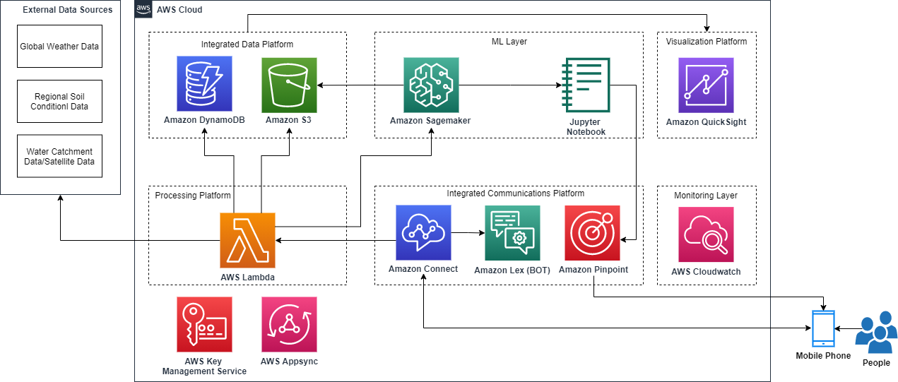
Team “Sustainable Force 99,” worked to better understand natural disasters, which have tripled over recent years. Their solution aims to predict natural disasters by analyzing the geographical spread of contributing factors like extreme weather due to climate change, wildfires, and deforestation. Then it communicates clear instructions to people who are potentially in danger.

Their solution (Figure 2) uses the Amazon SageMaker AI prediction model and combines The Weather Company data with Amazon S3, Amazon DynamoDB, and Serverless on AWS technologies and communicates with the public by:

  • Providing voice and chat communication channels using Amazon Connect, Amazon Lex, and Amazon Pinpoint.
  • Broadcasting alerts across smartphones and speakers in towns to provide information to people about upcoming natural disasters.
  • Allowing individuals to notify emergency services of their circumstances.
Local emergency communication system

Figure 2. Local emergency communication system

This communication helps governments and local authorities identify and communicate safe relocation options during disasters and connect with nearby relocation assistance teams.

Architecture 3: Intelligent satellite image processing

Team “Green Fire” examined how to reduce environmental problems caused by wildfires.

Many forest service organizations already use predictive tools to provide intelligence to fire services authorities using satellite imaging. The satellites can detect and capture images of wildfires. However, it can take hours to process these images and transmit and analyze the information, which can mean the subsequent coordination and mobilization of emergency services can be challenging.

To help improve fire rescue and other emergency services coordination and real-time situational awareness, Green Fire created a serverless application architecture (Figure 3):

  • The drone images, external data feeds from AWS Open Data Registry, and the datasets from The Weather Company are stored in Amazon S3 for processing.
  • AWS Lambda processes the images and resizes the data, and the outputs are stored in DynamoDB.
  • Rekognition labels the drone images that identify geographical risks and fire hazards. This allows emergency services to identify potential risks, and they can further model the potential spread of the wildfire and identify options to suppress it.
  • Lambda integrates the API layer between the web user interface and DynamoDB so users can access the application from a web browser/mobile device (mobile application developed using AWS Amplify). Amazon Cognito authenticates users and controls user access.
Intelligent image processing

Figure 3. Intelligent image processing

The team expects this solution to help prevent loss of human lives, save approximately 10% of yearly spend, and reduce CO2 emissions globally between 1.75 to 13.5 billion metric tons of carbon.

Architecture 4: Machine-learning-based solution to predict bee colonies at risk

Variations in vegetation, rising temperatures, and use of pesticide are significantly destroying habitats and creating inhospitable conditions for many species of bees. Over the last decade, beehives in the US and Europe have suffered hive losses of at least 30%.

To encourage the adoption of sustainable agriculture, it is important to safeguard bee colonies. The “I BEE GREEN” team developed a device that contains sensors that monitor beehive health, such as temperature, humidity, air pollutants, beehive acoustic signals, and the number of bees:

  • AWS IoT Core for LoRaWAN connects wireless sensor devices that use the LoRaWAN protocol for low-power, long-range comprehensive area network connectivity.
  • The sensor and weather data (from AWS Open Data Registry/The Weather Company) are loaded in Amazon S3 and transformed using AWS Glue.
  • Once the data is processed and ready to be consumed, it is stored on the AWS S3 bucket.
  • SageMaker consumes this data and generates forecasts such as estimated bee population and mortality rates, probability of infectious diseases and their spread, and the effect of the environment on beehive health.
  • The forecasts are presented in a dashboard using AWS QuickSight and are based on historical data, current data, and trends.

The information this solution generates can be used for several use cases, including:

  • Offering agricultural organizations information on how climate change impacts bee colonies and influences their business performance
  • Contributing to beekeepers’ understanding of the best environment to safeguard bee biodiversity and when to pollinate crops
  • Educating farmers on sustainable methods of agriculture that reduces threat to bees

The I BEE GREEN device automatically counts when bees are entering or exiting the hive. Using this, farmers can assess a hive’s acoustic signal, temperature, humidity, the presence of pollutants, classify them as normal or abnormal, and forecast the potential risk of abnormal mortality. The I BEE GREEN team aims for their device to deploy quickly, with minimal instructions anyone can implement.

Machine-learning-based architecture to predict bee colonies at risk

Figure 4. Machine-learning-based architecture to predict bee colonies at risk

Conclusion

In this blog post, we showed you how IBM hackathon teams used AWS technologies to solve sustainability-related challenges.

Ready to make your own? Visit our sustainability page to learn more about AWS services and features that encourage innovation to solve real-world sustainability challenges. Read more sustainability use cases on the AWS Public Sector Blog.

Make your monorepo feel small with Git’s sparse index

Post Syndicated from Derrick Stolee original https://github.blog/2021-11-10-make-your-monorepo-feel-small-with-gits-sparse-index/

One way that Git scales to the largest monorepos is the sparse-checkout feature, which allows you to focus on a subset of the files. This is supposed to make it feel like you are actually in a small repository, even though you are contributing to a large repository.

There’s only one problem: the Git index is still large in a monorepo, and users can feel it. Until now.

The Git index is a critical data structure in Git. It serves as the “staging area” between the files you have on your filesystem and your commit history. When you run git add, the files from your working directory are hashed and stored as objects in the index, leading them to be “staged changes”. When you run git commit, the staged changes as stored in the index are used to create that new commit. When you run git checkout, Git takes the data from a commit and writes it to the working directory and the index.

The working directory, index, and commit history

In addition to storing your staged changes, the index also stores filesystem information about your working directory. This helps Git report changed files more quickly. One problem is that the index stores this information for every file at HEAD, even if those files are outside of the sparse-checkout definition. This means that the index can be much larger in a monorepo than it would be if your important subset of files was in its own repository.

Throughout the past year, the Git Fundamentals team at GitHub contributed a new feature to Git called the sparse index, which allows the index to focus on the files within the sparse-checkout cone. If you are in a repository that can use sparse-checkout, then you can enable the sparse index using these commands:

git sparse-checkout init --cone --sparse-index
git sparse-checkout set <dir1> <dir2> ... <dirN>

The size of the sparse index will scale with the number of files within your chosen directories, instead of the full size of your repository. When enabled with a number of other performance features, this can have a dramatic performance impact.

As we built the sparse index, we tested its performance against a large monorepo that has over two million files at HEAD, and with a sparse-checkout definition that populated the working directory with about 100,000 of those files. We then compared the performance between having a normal “full” index, a sparse index, and a repository that only contained the files matching the sparse-checkout definition.

Command performance by index and repository type

The chart above demonstrates the significant performance improvements enabled by the sparse index. The bottom bars for each Git command show the runtime without the sparse index. The middle bars show the runtime of the same commands with the sparse index enabled. The top bars show the runtime of these commands, except in a repository that only contained the files within the sparse-checkout cone, representing the theoretical optimum. Since the sparse index still contains pointers to the rest of the monorepo, there is still some overhead. This overhead is hardly noticeable, since the difference is at most 60 milliseconds, even in the worst case above.

Today, I will go deep into the design and implementation of the sparse index. In particular, I’ll focus on how the Git community made such a significant change to a critical data structure in a safe way. I will include links to the actual changes in the Git codebase as I go.

This post is going to go deep into the guts of Git. If you are unfamiliar with Git’s object model, then learn about commits, trees, and blobs before continuing.

You can also get an overview of the sparse index alongside several other advanced Git features in this presentation I gave with colleague Lessley Dennington at the GitHub Nova event.

First, let’s dig into the Git index to understand its structure and purpose. I’ll use the derrickstolee/trace2-flamechart repository as a concrete example (and to generate some of the figures). If you want to follow along with the Git commands shown, then clone that repository.

The Git index

The index file stores a list of every file at HEAD, along with the object ID for its blob and some metadata. This list of files is stored as a flat list and Git parses the index into an array.

You can expose the list of files in the index using the git ls-files command:

$ git ls-files
LICENSE
README.md
bin/index.js
examples/fetch/git-fetch-after.png
examples/fetch/git-fetch-after.svg
examples/fetch/git-fetch-after.txt
examples/fetch/git-fetch-before.png
examples/fetch/git-fetch-before.svg
examples/fetch/git-fetch-before.txt
examples/fetch/git-fetch-combined.png
examples/fetch/git-fetch-combined.svg
examples/maintenance/trace.png
examples/maintenance/trace.svg
examples/maintenance/trace.txt
package.json

In this repository, many of the files live in an examples/ directory, but you don’t actually need them for the functionality of the code, which lives in the bin/ directory. You can focus the repository only on the necessary files using the git sparse-checkout command:

$ ls
LICENSE     README.md     bin       examples   package.json
$ git sparse-checkout init --cone --sparse-index
$ git sparse-checkout set bin
$ ls
LICENSE     README.md     bin       package.json

Even though I used the sparse-checkout command to reduce the size of the working directory, my git ls-files command will return the same set of files as before. In fact, I can dig in a little more and expose some more information using git ls-files --debug.

$ git ls-files --debug
LICENSE
  ctime: 1634910503:287405820
  mtime: 1634910503:287405820
  dev: 16777220 ino: 119325319
  uid: 501  gid: 20
  size: 1098    flags: 0
README.md
  ctime: 1634910503:288090279
  mtime: 1634910503:288090279
  dev: 16777220 ino: 119325320
  uid: 501  gid: 20
  size: 934 flags: 0
bin/index.js
  ctime: 1634910767:828434033
  mtime: 1634910767:828434033
  dev: 16777220 ino: 119325520
  uid: 501  gid: 20
  size: 7292    flags: 0
examples/fetch/git-fetch-after.png
  ctime: 0:0
  mtime: 0:0
  dev: 0    ino: 0
  uid: 0    gid: 0
  size: 0   flags: 40004000
(...)

The above output is truncated, but it shows that each index entry contains additional filesystem information for each path. The last entry listed shows what happens for a file that is outside of the sparse-checkout definition: all of the filesystem information is removed and the flags entry has some bits enabled. These bits include a SKIP_WORKTREE bit that signifies that Git will not write that file to the working directory.

If these files are not written to disk, then why are they listed in the index at all? The reason is that Git still needs to understand the content that would be there if the index was expanded. Further, that information is used to generate a commit with the git commit command.

In the Git codebase, there is a test helper that can show additional information from the index: test-tool read-cache. (You won’t have this command if you just have normal Git installed.) Running it here, you can see that the index also stores the object IDs for every file:

$ test-tool read-cache --table
100644 blob 646521d0d6c070e6f15e0f5828be1127d3b75503    LICENSE
100644 blob b230b3a6e2d81d50dc00177e970a10726b5baf08    README.md
100755 blob 918533d51c7a5f91622311893dcfd40bfd4f43d7    bin/index.js
100644 blob e0f88531b916b92821476760672e8161b9954898    examples/fetch/git-fetch-after.png
100644 blob f4a523cd1acb0a9d2620970ad7a43405d6e305dc    examples/fetch/git-fetch-after.svg
100644 blob fc4e30dca5fcb0c3d2031dc82a43d5d644e26b41    examples/fetch/git-fetch-after.txt
100644 blob 15dc889965617df3b5a30cf01e52c491e41c59c1    examples/fetch/git-fetch-before.png
100644 blob 602bd5bcbd815914a035d0d4f0d2a3896f600de2    examples/fetch/git-fetch-before.svg
100644 blob bc40a8e4658d17c35de996f3655e737b85ce7ad9    examples/fetch/git-fetch-before.txt
100644 blob 356cdd36e0d78a62af8b010d25d658054bb6fdc7    examples/fetch/git-fetch-combined.png
100644 blob cc0c23f2c8a822c51a17c46268f38c2268b400ae    examples/fetch/git-fetch-combined.svg
100644 blob dfc0893d172d841d971e206461466db935b7c192    examples/maintenance/trace.png
100644 blob a10a876472e46c6ae58e6fc6e2adc64d4dae809b    examples/maintenance/trace.svg
100644 blob 8f5e8bfbc44674feb3aa96e0b7bf1bf717495658    examples/maintenance/trace.txt
100644 blob a4599a9e0a01c28a2c0a622457664fc8c55bfdf9    package.json

Notice in particular how every single row lists the object type as blob, meaning a file. Also, the bin/index.js file has executable permissions, so the file permission column shows 100755 instead of 100644 like the others. This is all important metadata to store for each index entry.

To visualize the index, the diagram below displays our blobs as boxes in a line in the order given above, but it represents the trees that connect the root tree to those blobs as triangles. Thus, the root tree has two subtrees for bin/ and examples/, and the examples/ subtree has two subtrees for fetch/ and maintenance/.

full index

This figure represents all of the links between the trees and blobs. However, the core index data structure stores only the list of blobs as a flat list. The nesting tree structure does not exist in the core of the file.

However, there is an extension to the format that includes the information of the nesting directories: the cache-tree extension. Each node of the cache-tree stores a list of sub-nodes and a range of index entries that are covered by the current node. Each node stores the object ID for the tree it represents.

The index and the cache tree

The root node always covers all of the blobs in the index. The contained nodes have ranges contained within that range.

Git commands such as git add update the cache-tree extension in order to make the next git commit command very fast. To create the new commit, Git can use the tree from the root of the cache-tree extension.

Many Git commands use the index in many different ways. Some commands compare the working directory to the index and update one or the other when there is a difference. Others compare the index and a commit. Some compare multiple indexes together. Some use the cache-tree extension to navigate the nested tree structure, but mostly they scan the flat list of files in the form of an array.

The index affects Git performance at scale

The index can be very large in monorepos. I will show Git performance data from an example monorepo that has over two million files at HEAD. Even using the latest compression techniques available, the index file is over 180 MB in this monorepo.

This has a significant effect on normal Git commands. Presented below is an annotated flamechart of a git status command with one of these large indexes. The x-axis represents time since the start of the command, and each rectangle represents a region of Git’s execution that is marked by its trace2 logging library.

`git status` with full index

Three regions are annotated here:

  1. The index is read from disk and parsed into memory.
  2. The working directory is compared to the index. This triggers a lazy initialization of some hash tables that are required for this effort.
  3. The modified index is written to disk.

Parsing is multi-threaded, but writes are not. This explains some of the differences in how long those actions take.

Clearly, the amount of data in the index is a significant portion of this command. This also affects other commands such as git add and git commit, which are expected to be fast.

This performance concern became abundantly clear when our monorepo customer wanted to group more dependencies within the monorepo. Some teams had isolated Git repositories that were hundreds of times smaller than the monorepo, but these repositories created packages that were consumed by the monorepo, causing complications in tracking dependencies. The hope was that they could merge into the monorepo and rely on sparse-checkout to make it feel like they were still working in a small repository. The user experience was actually much worse, and the root cause was the time it took to read and write the index.

The main culprit is that there are millions of index entries corresponding to files these users do not care about for their daily work. When they push to the server and create a pull request, the build machines can handle the massive scale of building the entire tree and verifying that the small change works within the larger whole of the monorepo. Users should not need to pay that cost.

As members of the Git Fundamentals team, we are very focused on Git performance, and the index has been on our minds for years. For example, the index is a bottleneck for the VFS for Git environment, but that environment has particular needs that prevent improvements in this area.

The biggest thing that has changed recently is the creation of “cone mode” sparse-checkout patterns. These use directory-based pattern matching instead of file-based pattern matching. While cone mode was originally designed to speed up pattern matching in the sparse-checkout feature, it has now unlocked a new way to shrink the index.

The sparse index

The sparse index differs from a normal “full” index in one aspect: it can store directory paths with the object ID for its tree object. This is in addition to the file paths which are paired with blob objects. Since the cone mode sparse-checkout patterns match on a directory level, we can determine that an entire directory is out of the sparse-checkout cone and replace all of its contained file paths with a single directory path.

Back in my example derrickstolee/trace2-flamegraph repository, you can enable the sparse index command and then use the test-tool read-cache tool to show the contents of the index.

$ git sparse-checkout init --cone --sparse-index
$ test-tool read-cache --table
100644 blob 646521d0d6c070e6f15e0f5828be1127d3b75503    LICENSE
100644 blob b230b3a6e2d81d50dc00177e970a10726b5baf08    README.md
100755 blob 918533d51c7a5f91622311893dcfd40bfd4f43d7    bin/index.js
040000 tree b395192a7adbf21793f9489f3623c117802b2043    examples/
100644 blob a4599a9e0a01c28a2c0a622457664fc8c55bfdf9    package.json

Similar to my previous visualizations, you can now see how the index contains a directory entry in addition to the four blobs.

sparse index

The sparse directory entries correspond to directories that are just outside of the sparse-checkout definition. These directories also have a cache-tree node whose range is only one entry: that sparse directory entry.

I can even display the full details of the --debug output for git ls-files. This currently requires a --sparse flag that I have implemented in my personal fork of Git, but a similar feature will eventually be available in the core Git client.

$ git ls-files --debug --sparse
LICENSE
  ctime: 1634910503:287405820
  mtime: 1634910503:287405820
  dev: 16777220 ino: 119325319
  uid: 501  gid: 20
  size: 1098    flags: 200000
README.md
  ctime: 1634910503:288090279
  mtime: 1634910503:288090279
  dev: 16777220 ino: 119325320
  uid: 501  gid: 20
  size: 934 flags: 200000
bin/index.js
  ctime: 1634910767:828434033
  mtime: 1634910767:828434033
  dev: 16777220 ino: 119325520
  uid: 501  gid: 20
  size: 7292    flags: 200000
examples/
  ctime: 0:0
  mtime: 0:0
  dev: 0    ino: 0
  uid: 0    gid: 0
  size: 0   flags: 40004000
package.json
  ctime: 1634910503:288676330
  mtime: 1634910503:288676330
  dev: 16777220 ino: 119325321
  uid: 501  gid: 20
  size: 680 flags: 200000

This output is not truncated as it was before, and you can see that the sparse directory entry for examples/ is the only one with blank filesystem data. It also has the same flags value as the sparse file entries did before.

By removing the number of index entries as well as reducing the average path length, you can shrink the index size significantly. In our example monorepo, most users will reduce their index size from 180 MB to less than 10 MB!

Back to our monorepo, let’s try that git status example again and create a new flamechart. Here, I compare the flamechart for git status with a full index followed by one with a sparse index.

Annotated `git status` flame chart

With the sparse index, the git status command drops from 1.3 seconds to under 200 milliseconds! In the flame chart above I highlighted some regions that have similar appearance in each run. These represent the parts of the git status command that are actually walking the working directory and doing work independent of the index size. Everything else is slower in the full index case entirely because of the size of the index!

Building the sparse index safely

Pruning the index at the directory level is a relatively simple idea with a rather complicated result: our flat list of paths now contains two types of Git objects! There are dozens of places in the Git codebase that interact directly with the index in subtly different ways, and all of them are expecting every index entry to point to a blob object.

In order to make such a change to a critical data structure, we needed to first create a compatibility layer. To safely interact with a sparse index, we needed a way to expand a sparse index to an equivalent full index. This way, code paths that have not been integrated and tested with a sparse index can still be used, even if the on-disk format is sparse.

In the Git codebase, we started by creating the ensure_full_index() method, which converts a sparse index into a full one. This method inspects the list for directory entries and replaces them with its contained file entries. Since the directory is outside of the sparse-checkout cone, we could ignore all of the filesystem metadata information and populate the list by traversing the tree objects under that directory. Before anything else happens, the ensure_full_index() method is called immediately after parsing the index so no interactions with the index happen until the sparse directories are removed.

Expanding to a full index

When Git expands a sparse index to a full one, it scans the entries in lexicographic order. If the entry is a file, then Git copies it to the new list. If the entry is a directory, then the tree at that location is passed to the read_tree_at() method to iterate over all contained blobs. For each contained blob, Git generates an index entry for the corresponding file. Finally, the index entry list is copied back into the index and the index is no longer sparse.

Once that protection was in place, we extended Git to write the sparse index format. When writing the index, a full index is converted to a sparse one in-memory using the convert_to_sparse() method.

Collapsing to a sparse index

To convert from a full index to a sparse one, Git uses the cache-tree extension to find the object ID for our new sparse directory entries. The existing file entries are copied, and Git inserts the directory entries as needed.

Once these steps were built, we could verify that the index size was shrinking to the scale we expected. Both of these steps were included in a single series that introduced the format and implemented the conversions.

While it is nice that the index size has shrunk, we couldn’t stop there. The index is a very compact data structure, so it is more efficient to read it from disk than to recreate it by parsing trees. The ensure_full_index() method takes noticeably longer to expand a sparse index to a full one than it would take to read a full one from disk. In order to gain the performance benefits of a sparse index, we needed to teach Git what to do when encountering sparse directory entries.

Before embarking on these integrations, we first set up more guardrails. A new setting, command_requires_full_index, was created which is enabled by default. This setting is used to trigger ensure_full_index() upon parsing a sparse index unless the Git command being run has explicitly disabled the setting. This allowed us to integrate with Git commands one-by-one without disrupting the behavior of other Git commands. In addition to these settings, we inserted calls to ensure_full_index() before most index interactions. to make sure that we were operating on a full index in any code path that might iterate over the index entries. This allowed us to find which code paths needed integration: we could debug a Git command with a breakpoint on ensure_full_index() and see the call stack that led to that expansion.

The first command to integrate with the sparse index was git status. In hindsight, this was a challenging command to use as a starting point, because it performs multiple index operations that are common to other commands. This became clear when integrating with git checkout and git commit because most of the work was already done in the git status integration.

Let’s explore some of the smaller interactions that needed special care with directory entries.

Example implementation detail: git diff

The git diff command can show what is different between different representations of a working directory. There are two interesting cases that involve the index: comparing the working directory to the index, and comparing the index to a commit.

With no other arguments, git diff shows the differences in the working directory compared to what is staged in the index. This algorithm is mostly simple to integrate with the sparse index: while walking the working directory, Git drills into a directory only if it exists. If the sparse directory entries in the sparse index do not appear as directories in the working directory, then it never tries to drill into the sparse directory entries. If Git finds that a sparse directory entry does exist in the filesystem as a real directory, then the ensure_full_index() method expands the index and Git continues as normal. This is not desired, so we did everything possible to make sure that these directories do not exist, including updating the sparse-checkout feature to delete ignored files outside the cone.

The git diff --cached command compares the files staged in the index with the commit at HEAD. Here, it is easier to have differences outside the sparse-checkout cone, such as when using git reset --soft to change the HEAD commit without changing the working directory or index. In this case, the git diff --cached command wants to compare the root tree for the HEAD commit to the files in the index. This can proceed normally for the files that exist in the sparse index, but when we reach a sparse directory entry, we see the tree object staged in the index as well as a tree object from the tree walk. At this point, we shift from a tree-vs-index comparison to a tree-vs-tree comparison of those subtrees. When that diff is complete, we can continue with the larger comparison.

One major benefit to the tree-vs-tree comparison is that it is easier to compare the same type of objects. The recursive comparison can also prune the walk when it finds two subtrees with the same object ID, as all of their content is the same at that point.

This change allows us to report on these differences not only in the git diff command, but also such diffs as are written during git status, git checkout, and git commit.

Implementation detail: ORT merge strategy

When beginning the sparse index work, there was a huge question that we did not know how to tackle: three-way merges. The default merge strategy, recursive, uses the index as a data structure during its computation. It was going to be difficult to reconcile that algorithm to work within the confines of a sparse index. In fact, many merges that a monorepo user runs would need to resolve merges outside of the sparse-checkout cone.

Luckily, another contributor, Elijah Newren, announced that he was creating a new merge strategy, named the ORT strategy, that did not use the index. We prioritized reviewing and testing that strategy so that we could take advantage of it. It turns out that it is also a better algorithm in general, so it will become the new default strategy with Git 2.34.

The critical feature of the ORT strategy was its replacement of the index with a recursive tree-like structure. That structure is built from the root tree and only creates subtrees for paths that have changed since the merge base. At the end, the ORT strategy creates an index to match its representation of the resulting merge commit.

Because of the ORT merge strategy, integrating the sparse index into git merge, git rebase, git cherry-pick, and git revert was very simple. We just needed to make sure the index that was created at the end of the merge was sparse from its original creation.

Different merge strategies and their performance

As we reported earlier, the ORT strategy improves over the recursive strategy in the typical case, but also the recursive strategy has significant outliers as shown in the box plot above. Enabling the sparse index on top of the ORT strategy provides even more improvements.

Without the ORT merge strategy, the sparse index work could have easily doubled in scope. For a detailed look at the ORT strategy and its many optimizations, take a look at Elijah’s six-part blog series:

Testing the sparse index

The sparse index was touching critical code and doing so in interesting ways. We needed a way to carefully test that these changes were as correct as possible. The Git test suite is substantial and has excellent coverage of most index operations. However, almost all of those tests do not use sparse-checkout, so we couldn’t immediately gain value in checking the sparse index by enabling it globally.

We created a test script that focused on testing the sparse index in a new way. The test starts by creating a repository with some interesting data shapes in it. Then, each test case starts by copying that repository into three new repositories. Those three repositories have different configurations:

  1. The repository as-is, without sparse-checkout.
  2. The repository with cone mode sparse-checkout enabled.
  3. The repository with cone mode sparse-checkout and sparse index enabled.

Then, each test case runs a number of Git commands against all three repositories, expecting the same output and results in the working directory. This allowed us to be confident that the changes we were making to enable the sparse index would have identical behavior with the other two cases.

Along the way, we found some interesting differences between sparse-checkout and full repositories. Several of these bugs have been fixed since. Sometimes, it was unclear whether the sparse-checkout feature should do the same thing as a normal repository, specifically when interacting with files outside of the sparse-checkout cone. This led to changing how some commands interact with sparse entries. In Git 2.34, some commands will need a --sparse flag in order to modify paths outside of the sparse-checkout cone.

In addition to these test scripts, we routinely ran the Scalar functional tests against our development branches, since many of those tests focus on special circumstances around the sparse-checkout feature. If a Scalar test would fail when the Git tests did not, then we would create a similar test in Git to prevent such a bug in the future.

Once we had integrated with a core set of Git commands, we also created an experimental release that contained early versions of these integrations. We provided this version to a subset of monorepo users to evaluate the performance. We found some interesting data from some of the users, but overall the results confirmed that the sparse index was going to significantly improve the user experience in the monorepo. The most important thing we discovered is that the sparse-checkout feature should remove ignored files outside of the cone, as those files cause the sparse index to expand to a full one, negating the performance benefits. There is an additional benefit in that the working directory shrinks even more by deleting these files.

The current state of the sparse index

Not all Git commands understand the sparse index. Those that have not been integrated trigger a compatibility check that converts a sparse index into a full one during the first index read. The integrated commands are ones that have been carefully tested with the sparse index. They likely received some code updates in order to properly handle a sparse index. These integrations were dispersed across the last few Git versions, and some only exist in the microsoft/git fork until we can complete contributing them to the core Git project.

scope

In June, Git 2.32.0 was released with an understanding of the sparse index format. In August, Git 2.33.0 included integrations with git status, git commit, and git checkout. Git 2.34.0 is slated for a November release with integrations for git add, git merge, git rebase, git cherry-pick, and git reset. In order to serve our monorepo users, we fast-tracked some integrations into a pre-release in our fork including integrations with git diff, git blame, git clean, git sparse-checkout, and git stash.

Based on our understanding of how users interact with a monorepo, the commands that are listed here are sufficient to cover almost all users’ needs. We expect that users who adopt the sparse index with these integrations will have a significantly improved experience from before. This all depends on the size of their monorepo and on the size of their sparse-checkout cone.

We will release this feature widely to our monorepo users with the sparse index on by default in the 2.34 release of our Git fork. The core Git project will keep the sparse index off by default until it has all of these features and the implementation has been stable for a few versions.

Looking to the future

At this point, we have covered all of the integrations we need to have a successful monorepo experience. There is more work to be done. In particular, we need to finish contributing the final integrations in our list. Upstream progress takes time and we are grateful for all of the feedback we have received from the community so far. There are more commands that could use integrations, as well.

For now, we are focused on ensuring that monorepo users transition to the sparse index without incident. If you are interested in the sparse index, then we believe it is in an excellent state to start using it. If you have any issues with its performance or stability, then please do not hesitate to create an issue or start a discussion. We will be there to help!

Through the sparse index, we broke through a significant barrier to monorepo scale. We continue to seek the next innovation that will help Git scale to the largest repos out there.

CVE-2021-43287 Allows Pre-Authenticated Build Takeover of GoCD Pipelines

Post Syndicated from Caitlin Condon original https://blog.rapid7.com/2021/11/10/cve-2021-43287-allows-pre-authenticated-build-takeover-of-gocd-pipelines/

CVE-2021-43287 Allows Pre-Authenticated Build Takeover of GoCD Pipelines

On October 26, 2021, open-source CI/CD solution GoCD released version 21.3.0, which included a fix for CVE-2021-43287, a critical information disclosure vulnerability whose exploitation allows unauthenticated attackers to leak configuration information, including build secrets and encryption keys. Both Rapid7 vulnerability researchers and community researchers were easily able to register a rogue agent, injecting themselves into GoCD builds and enabling full, pre-authenticated pipeline takeover. CVE-2021-43287 can be exploited with a single HTTP request.

While CVE-2021-43287 is still awaiting a formal CVSSv3 score and description, it’s no secret that CI/CD tooling and pipelines are high-value targets for both sophisticated and opportunistic attackers. GoCD customers should update to version 21.3.0 on an emergency basis, given the potential for exploitation to undermine the integrity of their software development pipelines. The US Cybersecurity and Infrastructure Security Agency (CISA) has also issued an alert and patch guidance. Rapid7’s vulnerability research team has a more detailed technical analysis of CVE-2021-43287 here.

Rapid7 customers

InsightVM and Nexpose customers can assess their exposure to CVE-2021-43287 with a remote vulnerability check available in the November 9, 2021 content release.

NEVER MISS A BLOG

Get the latest stories, expertise, and news about security today.

The collective thoughts of the interwebz