The Amazon Titan family of models, available exclusively in Amazon Bedrock, is built on top of 25 years of Amazon expertise in artificial intelligence (AI) and machine learning (ML) advancements. Amazon Titan foundation models (FMs) offer a comprehensive suite of pre-trained image, multimodal, and text models accessible through a fully managed API. Trained on extensive datasets, Amazon Titan models are powerful and versatile, designed for a range of applications while adhering to responsible AI practices.
The latest addition to the Amazon Titan family is Amazon Titan Text Embeddings V2, the second-generation text embeddings model from Amazon now available within Amazon Bedrock. This new text embeddings model is optimized for Retrieval-Augmented Generation (RAG). It is pre-trained on 100+ languages and on code.
Amazon Titan Text Embeddings V2 now lets you choose the size of of the output vector (either 256, 512, or 1024). Larger vector sizes create more detailed responses, but will also increase the computational time. Shorter vector lengths are less detailed but will improve the response time. Using smaller vectors helps to reduce your storage costs and the latency to search and retrieve document extracts from a vector database. We measured the accuracy of the vectors generated by Amazon Titan Text Embeddings V2 and we observed that vectors with 512 dimensions keep approximately 99 percent of the accuracy provided by vectors with 1024 dimensions. Vectors with 256 dimensions keep 97 percent of the accuracy. This means that you can save 75 percent in vector storage (from 1024 down to 256 dimensions) and keep approximately 97 percent of the accuracy provided by larger vectors.
Amazon Titan Text Embeddings V2 also proposes an improved unit vector normalization that helps improve the accuracy when measuring vector similarity. You can choose between normalized or unnormalized versions of the embeddings based on your use case (normalized is more accurate for RAG use cases). Normalization of a vector is the process of scaling it to have a unit length or magnitude of 1. It is useful to ensure that all vectors have the same scale and contribute equally during vector operations, preventing some vectors from dominating others due to their larger magnitudes.
This new text embeddings model is well-suited for a variety of use cases. It can help you perform semantic searches on documents, for example, to detect plagiarism. It can classify labels into data-based learned representations, for example, to categorize movies into genres. It can also improve the quality and relevance of retrieved or generated search results, for example, recommending content based on interest using RAG.
How embeddings help to improve accuracy of RAG Imagine you’re a superpowered research assistant for a large language model (LLM). LLMs are like those brainiacs who can write different creative text formats, but their knowledge comes from the massive datasets they were trained on. This training data might be a bit outdated or lack specific details for your needs.
This is where RAG comes in. RAG acts like your assistant, fetching relevant information from a custom source, like a company knowledge base. When the LLM needs to answer a question, RAG provides the most up-to-date information to help it generate the best possible response.
To find the most up-to-date information, RAG uses embeddings. Imagine these embeddings (or vectors) as super-condensed summaries that capture the key idea of a piece of text. A high-quality embeddings model, such as Amazon Titan Text Embeddings V2, can create these summaries accurately, like a great assistant who can quickly grasp the important points of each document. This ensures RAG retrieves the most relevant information for the LLM, leading to more accurate and on-point answers.
Think of it like searching a library. Each page of the book is indexed and represented by a vector. With a bad search system, you might end up with a pile of books that aren’t quite what you need. But with a great search system that understands the content (like a high-quality embeddings model), you’ll get exactly what you’re looking for, making the LLM’s job of generating the answer much easier.
Amazon Titan Text Embeddings V2 overview Amazon Titan Text Embeddings V2 is optimized for high accuracy and retrieval performance at smaller dimensions for reduced storage and latency. We measured that vectors with 512 dimensions maintain approximately 99 percent of the accuracy provided by vectors with 1024 dimensions. Those with 256 dimensions offer 97 percent of the accuracy.
Max tokens
8,192
Languages
100+ in pre-training
Fine-tuning supported
No
Normalization supported
Yes
Vector size
256, 512, 1,024 (default)
How to use Amazon Titan Text Embeddings V2 It’s very likely you will interact with Amazon Titan Text Embeddings V2 indirectly through Knowledge Bases for Amazon Bedrock. Knowledge Bases takes care of the heavy lifting to create a RAG-based application. However, you can also use the Amazon Bedrock Runtime API to directly invoke the model from your code. Here is a simple example in the Swift programming language (just to show you you can use any programming language, not just Python):
import Foundation
import AWSBedrockRuntime

let text = "This is the text to transform in a vector"

// create an API client
let client = try BedrockRuntimeClient(region: "us-east-1")

// create the request
let request = InvokeModelInput(
   accept: "application/json",
   body: """
   {
      "inputText": "\(text)",
      "dimensions": 256,
      "normalize": true
   }
   """.data(using: .utf8),
   contentType: "application/json",
   modelId: "amazon.titan-embed-text-v2:0")

// send the request
let response = try await client.invokeModel(input: request)

// decode the response
let response = String(data: (response.body!), encoding: .utf8)

print(response ?? "")
The model takes three parameters in its payload:
inputText – The text to convert to embeddings.
normalize – A flag indicating whether or not to normalize the output embeddings. It defaults to true, which is optimal for RAG use cases.
dimensions – The number of dimensions the output embeddings should have. Three values are accepted: 256, 512, and 1024 (the default value).
I added the dependency on the AWS SDK for Swift in my Package.swift. I type swift run to build and run this code. It prints the following output (truncated to keep it brief):
Amazon Titan Text Embeddings V2 will soon be the default LLM proposed by Knowledge Bases for Amazon Bedrock. Your existing knowledge bases created with the original Amazon Titan Text Embeddings model will continue to work without changes.
To learn more about the Amazon Titan family of models, view the following video:
The new Amazon Titan Text Embeddings V2 model is available today in Amazon Bedrock in the US East (N. Virginia) and US West (Oregon) AWS Regions. Check the full Region list for future updates.
Editors note April 30, 2024: The information in this post is outdated and the solution has been retired. For more solutions using AWS services, see the AWS Solutions Library.
The new version of the AWS Ops Automator, a solution that enables you to automatically manage your AWS resources, features vertical scaling for Amazon EC2 instances. With vertical scaling, the solution automatically adjusts capacity to maintain steady, predictable performance at the lowest possible cost. The solution can resize your instances by restarting your existing instance with a new size. Or, the solution can resize your instances by replacing your existing instance with a new, resized instance.
With this update, the AWS Ops Automator can help make setting up vertical scaling easier. All you have to do is define the time-based or event-based trigger that determines when the solution scales your instances, and choose whether you want to change the size of your existing instances or replace your instances with new, resized instances. The time-based or event-based trigger invokes the AWS Lambda to scale your instances.
Restarting with a new size
When you choose to resize your instances by restarting the instance with a new size, the solution increases or decreases the size of your existing instances in response to changes in demand or at a specified point in time. The solution automatically changes the instance size to the next defined size up or down.
Replacing with a new, resized instance
Alternatively, you can choose to have the Ops Automator replace your instance with a new, resized instance instead of restarting your existing instance. When the solution determines that your instances need to be scaled, the solution launches new instances with the next defined instance size up or down. The solution is also integrated with Elastic Load Balancing to automatically register the new instance with load Balancers.
Editor’s note: Editor’s note: This post has been updated since it was last published in 2021.
Synology network attached storage (NAS) devices are great for businesses. They enable easy collaboration, speed up restores, make your files accessible 24/7, and give you a level of data protection you probably didn’t have before. Essentially, a NAS device acts as a private cloud, offering centralized access and storage for everything from large files to ongoing projects.
That’s why it’s important to back up your Synology DiskStation to the cloud. While NAS offers a layer of redundancy on-premises if you happen to lose files, it doesn’t fully protect you from things like a natural disaster, a ransomware attack that infiltrates your backups, or multiple hard drive failures. Cloud backups are important for data redundancy and future data recovery, giving you easy access and fast restores.
To keep your data truly safe, the 3-2-1 backup strategy is the industry baseline. Using a 3-2-1 strategy with your NAS means you keep three copies of your data on two different media (like NAS and cloud storage), with one stored off-site. Backing your DiskStation up to the cloud is a great way to achieve that key off-site element. This setup protects against various risks, and ensures your data is available for recovery.
In this post, we’ll explain how to implement a 3-2-1 backup strategy for your Synology NAS, the benefits of backing up to cloud storage, options for backing up your DiskStation, and some practical examples of what you can do by pairing your NAS with cloud storage.
Synology NAS and a 3-2-1 Backup Strategy
The 3-2-1 backup strategy is simple and time-tested. If you are using your Synology NAS to connect and back up computers on your network, that’s the first step—you have two local copies of your data on different mediums. You’d accomplish this by creating a multi-version local copy.
While this setup might seem sufficient, your data is still at risk from NAS device failure. It remains co-located with your primary data, making it vulnerable to disasters or theft. To fully protect your data, you need a third, off-site backup copy.
For your third copy, you could back up your Synology to an external desFor your third copy, you could back up your Synology to an external destination—either another Synology NAS, a file server, or a USB device. Each has pros and cons, and we’ll talk through them for argument’s sake.
Back up to another Synology NAS: If you recently upgraded to a new device, you could store the third copy of your data on your old DiskStation. You get to put the old one to use, and you know it’s compatible.
Back up to a file server: Backing your Synology NAS up to a file server is also an option, but it will take up more storage space for caching than backing up to another DiskStation.
Back up to a USB device: Backing up to a USB device has some limited advantages—the format of your data is readable, so you can plug the USB in anywhere and access your data. However, USB backup won’t back up applications or system files, and it’s a manual rather than an automated process.
With any of these options, you’ll need to physically move your backup device—the old Synology, file server, or USB-connected device—to another location, ideally more than a few miles away, to truly achieve a 3-2-1 backup.
However, backing up your Synology NAS DiskStation to the cloud means you achieve a 3-2-1 strategy without the need to physically separate your backup copies. Backing up your Synology NAS to the cloud means you have both convenience and robust data redundancy.
The Benefits of Backing Up Your Synology DiskStation to the Cloud
In addition to avoiding the lift of a physical move, backing up Synology NAS to the cloud offers a number of other benefits, too, including:
Avoiding data loss: A cloud backup protects against physical disasters, such as floods, hurricanes, and fires, that could compromise your NAS and data on individual workstations. Because the NAS is always connected to your machines, it’s also at risk of infection from ransomware attacks. And finally, the hard drives in your NAS can fail. Because your NAS is likely set up in a RAID configuration, one drive failure might not affect your data. But, while one drive is down, your data is at a higher risk. If another drive were to fail, you could lose data. Having an off-site backup in cloud storage significantly reduces this risk.
Accessibility: With your data in the cloud, your backups are accessible from anywhere. If you’re away from your desk or office and you need to retrieve a file, you can simply log in to your cloud instance and retrieve it remotely.
Security: Cloud vendors typically protect customer data by encrypting it as it travels to its final destination and/or when it’s at rest on the vendors’ storage servers. Encryption protocols differ between cloud vendors, so make sure to understand them as you’re evaluating cloud providers, especially if your organization has specific security requirements.
Automation: Your Synology NAS comes with built-in backup utilities, so you can configure a backup schedule for automated cloud backups . This saves time and ensures your data is always up-to-date.
Scalability: As your data grows, your cloud backups grow with it. With cloud storage, there’s no need to invest in or maintain additional hardware to ensure your data is properly backed up.
Rapid Data Recovery: Cloud storage often offers shorter recovery times than traditional methods, particularly if your NAS device fails or data needs to be restored urgently. Cloud storage solutions can streamline data retrieval, allowing quick access to backed-up files and minimizing downtime.
Multi-Cloud Options: Many cloud providers support multi-cloud setups, allowing you to back up your Synology NAS to multiple cloud destinations. This added redundancy can be a valuable safeguard against any single provider outages, helping to ensure continuous data availability.
File Versioning: Some cloud storage services support file versioning, which is the ability to keep previous versions of files. This is particularly useful if files are accidentally modified or deleted. It can help you restore earlier versions without losing valuable information.
Options for Backing Up Your Synology NAS
Synology offers various backup utilities and methods to protect your data, each suited to different backup needs and environments.
1. Hyper Backup
Hyper Backup is Synology’s built-in backup utility for backing up to any number of external destinations, including public clouds. It enables you to back up not just data stored on your NAS, but also applications and system configurations.
It offers incremental backups to help you manage your storage footprint. After your initial backup, using incremental backups means only files that have been changed will be updated.
It also offers cross-file deduplication to help you further manage your storage footprint. Hyper Backup allows you to back up to external devices as well as cloud services.
2. Cloud Sync
In addition to Hyper Backup, Synology also offers Cloud Sync, which is important for those who need real-time collaboration and file syncing capabilities. Keep in mind that sync is not the same as backup–Cloud Sync does not support application and system configuration file backups, and it only keeps the current version of your files. If someone accidentally deletes that file, it’s gone. If you’re not sure if you’re looking for backup or sync, you can read about the differences between them in this post.
3. Snapshot replication
If your Synology model supports the Btrfs file system, using Snapshot Replication is a bit faster both on the backup side and the restore side than Hyper Backup. Snapshot Replication allows you to back up to the same Synology NAS or another Synology NAS, but not to the cloud.
4. USB copy
USB Copy only copies your data, not applications or system configuration files. It does not support cross-file deduplication, so you might end up with duplicate copies of your files. Additionally, this method is manual, and will require you to be responsible for regular backups as opposed to automating them with Hyper Backup or Snapshot Replication.
What You Can Do With Cloud Sync, Hyper Backup, and Cloud Storage
Using Hyper Backup and Cloud Sync together gives you total control over what gets backed up to cloud storage—you can synchronize in the cloud as little or as much as you want. This flexible approach allows you to customize your backup plan and protect your Synology NAS data based on priority and needs.
Here are some practical examples of what you can do with Cloud Sync, Hyper Backup, and cloud storage working together.
1. Sync or Back Up the Entire Contents of Your DiskStation to the Cloud
The DiskStation has excellent fault-tolerance—it can continue operating even when individual drive units fail. However, for comprehensive protection, syncing and backing up the entire DiskStation to cloud storage ensures that your data remains secure during a disaster or system failure.
2. Sync or Back Up Your Most Important Media Files
If you’re storing essential media files—like videos, music, and photos—on your DiskStation, Cloud Sync or Hyper Backup can ensure these valuable files are safely stored in the cloud. Synology NAS offers data redundancy on-premises, but cloud storage provides an additional off-site backup layer for further protection.
3. Back Up Time Machine
For Mac operations, Synology allows the DiskStation to serve as a network-based Time Machine backup. With Hyper Backup, you can synchronize Time Machine files to the cloud so that in the event of a critical failure, your Time Machine backups are securely stored off-site, ready for a seamless restoration.
Ready to Give It a Try?
Hyper Backup allows you to choose from any number of cloud storage providers as a backup destination, and Backblaze B2 Cloud Storage is one of them.If you haven’t given cloud storage a try yet, you can get started now, and make sure your NAS is synced or backed up securely to the cloud.
FAQs About Synology NAS
How do I back up my Synology NAS to the cloud?
Hyper Backup is Synology’s built-in backup utility for backing up to any number of external destinations, including public clouds. It enables you to back up not just data stored on your NAS, but also applications and system configurations. Additionally, It offers cross-file deduplication to help you further manage your storage footprint and avoid duplicates.
What’s the best way to back up my Synology NAS?
Synology offers a lot of options for backing up your device, including to local volumes, external devices, other Synology systems, rsync servers, or public cloud services like Backblaze B2. The best way to back up your Synology NAS depends on many different factors, but the most important thing to remember is that you should follow a 3-2-1 backup strategy. That means keeping three copies of your data on two different media (i.e. devices) with one off-site. Backing up to the cloud is a great option for data redundancy and long-term protection when handling your off-site backups.
Can I schedule automatic cloud backups from my Synology NAS?
Yes, with Hyper Backup, you can set up automatic backups to many public clouds, including Backblaze B2. It offers incremental backups to help you manage your storage footprint. After your initial backup, using incremental backups means only files that have been changed will be updated.
Which cloud storage providers are compatible with Synology NAS for backup?
Synology is compatible with many public cloud providers, including Backblaze B2, Microsoft Azure, Google Cloud Platform, Amazon S3, and Synology C2 Storage.
How much cloud storage space do I need for my Synology NAS backup?
The amount of cloud storage space needed for your Synology NAS backup depends on factors like the total data size, frequency of backups, and retention policies. Calculate your NAS data size, estimate growth, and choose a cloud plan accordingly. Hyper Backup provides storage estimates, helping you select the right amount of cloud storage space for secure, scalable data backups.
When it comes to security, telling developers to do (or not do)
something can be ineffective. Helping them understand the why behind
instructions, by illustrating good and bad practices using stories, can be
much more effective. With several such stories Marta
Rybczyńska fashioned an interesting talk
about patterns and anti-patterns in embedded Linux security at the Embedded
Open Source Summit (EOSS), co-located with Open
Source Summit North America (OSSNA), on April 16 in Seattle, Washington.
Rapid7 is very excited to announce that version 0.7.2 of Velociraptor is now fully available for download.
In this post we’ll discuss some of the interesting new features.
EWF Support
Velociraptor has introduced the ability to analyze dead disk images in the past. Although we don’t need to analyze disk images very often, it comes up occasionally.
Previously, Velociraptor only supported analysis of DD images (AKA “Raw images”). Most people use standard acquisition software to acquire images, which uses the common EWF format to compress them.
In this 0.7.2 release, Velociraptor supports EWF (AKA E01) format using the ewf accessor. This allows Velociraptor to analyze E01 image sets.
To analyze dead disk images use the following steps:
Create a remapping configuration that maps the disk accessors into the E01 image. This automatically diverts VQL functions that look at the filesystem into the image instead of using the host’s filesystem. In this release you can just point the –add_windows_disk option to the first disk of the EWF disk set (the other parts are expected to be in the same directory and will be automatically loaded). The following creates a remapping file by recognizing the windows partition in the disk image.
2. Next we launch a client with the remapping file. This causes any VQL queries that access the filesystem to come from the image instead of the host. Other than that, the client looks like a regular client and will connect to the Velociraptor server just like any other client. To ensure that this client is unique you can override the writeback location (where the client id is stored) to a new file.
Sometimes we can’t deploy the Velociraptor client on a remote system. (For example, it might be an edge device like an embedded Linux system or it may not be directly supported by Velociraptor.)
In version 0.7.1, Velociraptor introduced the ssh accessor which allows VQL queries to use a remote ssh connection to access remote files.
This release added the ability to apply remapping in a similar way to the dead disk image method above to run a Virtual Client which connects to the remote system via SSH and emulates filesystem access over the sftp protocol.
To use this feature you can write a remapping file that maps the ssh accessor instead of the file and auto accessors:
remappings:
type: permissions
permissions:
COLLECT_CLIENT
FILESYSTEM_READ
READ_RESULTS
MACHINE_STATE
type: impersonation
os: linux
hostname: RemoteSSH
type: mount
scope: |
LET SSH_CONFIG <= dict(hostname=’localhost:22′,
username=’test’,
private_key=read_file(filename=’/home/test/.ssh/id_rsa’))
from:
accessor: ssh
"on":
accessor: auto
path_type: linux
type: mount
scope: |
LET SSH_CONFIG <= dict(hostname=’localhost:22′,
username=’test’,
private_key=read_file(filename=’/home/test/.ssh/id_rsa’))
from:
accessor: ssh
"on":
accessor: file
path_type: linux
Now you can start a client with this remapping file to virtualize access to the remote system via SSH.
The GUI has been significantly improved in this release.
Undo/Redo for notebook cells
Velociraptor offers an easy way to experiment and explore data with VQL queries in the notebook interface. Naturally, exploring the data requires going back and forth between different VQL queries.
In this release, Velociraptor keeps several versions of each VQL cell (by default 5) so as users explore different queries they can easily undo and redo queries. This makes exploring data much quicker as you can go back to a previous version instantly.
Hunt view GUI is now paged
Previously, hunts were presented in a table with limited size. In this release, the hunt table is paged and searchable/sortable. This brings the hunts table into line with the other tables in the interface and allows an unlimited number of hunts to be viewable in the system.
Secret Management
Many Velociraptor plugins require secrets to operate. For example, the ssh accessor requires a private key or password to log into the remote system. Similarly the s3 or smb accessors require credentials to upload to the remote file servers. Many connections made over the http_client() plugin require authorization – for example an API key to send Slack messages or query remote services like Virus Total.
Previously, plugins that required credentials needed those credentials to be passed as arguments to the plugin. For example, the upload_s3() plugin requires AWS S3 credentials to be passed in as parameters.
This poses a problem for the Velociraptor artifact writer: how do you safely provide the credentials to the VQL query in a way that does not expose them to every user of the Velociraptor GUI? If the credentials are passed as parameters to the artifact then they are visible in the query logs and request, etc.
This release introduces Secrets as a first class concept within VQL. A Secret is a specific data object (key/value pairs) given a name which is used to configure credentials for certain plugins:
A Secret has a name which we use to refer to it in plugins.
Secrets have a type to ensure their data makes sense to the intended plugin. For example a secret needs certain fields for consumption by the s3 accessor or the http_client() plugin.
Secrets are shared with certain users (or are public). This controls who can use the secret within the GUI.
The GUI is careful to not allow VQL to read the secrets directly. The secrets are used by the VQL plugins internally and are not exposed to VQL users (like notebooks or artifacts).
Let’s work through an example of how Secrets can be managed within Velociraptor. In this example we store credentials for the ssh accessor to allow users to glob() a remote filesystem within the notebook.
First we will select manage server secrets from the welcome page.
Next we will choose the SSH PrivateKey secret type and add a new secret.
This will use the secret template that corresponds to the SSH private keys. The acceptable fields are shown in the GUI and a validation VQL condition is also shown for the GUI to ensure that the secret is properly populated. We will name the secret DevMachine to remind us that this secret allows access to our development system. Note that the hostname requires both the IP address (or dns name) and the port.
Next we will share the secrets with some GUI users
We can view the list of users that are able to use the secret within the GUI
Now we can use the new secret by simply referring to it by name:
Not only is this more secure but it is also more convenient since we don’t need to remember the details of each secret to be able to use it. For example, the http_client() plugin will fill the URL field, headers, cookies etc directly from the secret without us needing to bother with the details.
WARNING: Although secrets are designed to control access to the raw credential by preventing users from directly accessing the secrets’ contents, those secrets are still written to disk. This means that GUI users with direct filesystem access can simply read the secrets from the disk.
We recommend not granting untrusted users elevated server permissions like EXECVE or Filesystem Read as it can bypass the security measures placed on secrets.
Server improvements
Implemented Websocket based communication mechanism
One of the most important differences between Velociraptor and some older remote DFIR frameworks such as GRR is the fact that Velociraptor maintains a constant, low latency connection to the server. This allows Velociraptor clients to respond immediately without needing to wait for polling on the server.
In order to enhance compatibility between multiple network configurations like MITM proxies, transparent proxies etc., Velociraptor has stuck to simple HTTP based communications protocols. To keep a constant connection, Velociraptor uses the long poll method, keeping HTTP POST operations open for a long time.
However as the Internet evolves and newer protocols become commonly used by major sites, the older HTTP based communication method has proven more difficult to use. For example, we found that certain layer 7 load balancers interfere with the long poll method by introducing buffering to the connection. This severely degrades communications between client and server (Velociraptor falls back to a polling method in this case).
On the other hand, modern protocols are more widely used, so we found that modern load balancers and proxies already support standard low latency communications protocols such as Web Sockets.
In the 0.7.2 release, Velociraptor introduces support for websockets as a communications protocol. The websocket protocol is designed for low latency and low overhead continuous communications methods between clients and server (and is already used by most major social media platforms, for example). Therefore, this new method should be better supported by network infrastructure as well as being more efficient.
To use the new websocket protocol, simply set the client’s server URL to have wss:// scheme:
You can use both https and wss URLs at the same time, Velociraptor will switch from one to the other scheme if one becomes unavailable.
Dynamic DNS providers
Velociraptor has the capability to adjust DNS records by itself (AKA Dynamic DNS). This saves users the hassle of managing a dedicated dynamic DNS service such as ddclient).
Traditionally we used Google Domains as our default Dynamic DNS provider, but Google has decided to shut down this service abruptly forcing us to switch to alternative providers.
The 0.7.2 release has now switched to CloudFlare as our default preferred Dynamic DNS provider. We also added noip.com as a second option.
Setting up CloudFlare as your preferred dynamic DNS provider requires the following steps:
You will need to require the “Edit” permission on Zone DNS and include the specific zone name you want to manage. The zone name is the domain you purchased, e.g. “example.com”. You will be able to set the hostname under that domain, e.g. “velociraptor.example.com”.
Using this information you can now create the dyndns configuration:
Make sure the Frontend.Hostname field is set to the correct hostname to update – for example
Frontend:
hostname: velociraptor.example.com
This is the hostname that will be updated.
Enhanced proxy support
Velociraptor is often deployed into complex enterprise networks. Such networks are often locked down with complicated controls (such as MITM inspection proxies or automated proxy configurations) which Velociraptor needs to support.
Velociraptor already supports MITM proxies but previously had inflexible proxy configuration. The proxy could be set or unset but there was no finer grained control over which proxy to choose for different URLs. This makes it difficult to deploy on changing network topologies (such as roaming use).
The 0.7.2 release introduces more complex proxy condition capabilities. It is now possible to specify which proxy to use for which URL based on a set of regular expressions:
By default connect to http://192.168.1.1:3128/ for all URLs (including https)
Except for www.google.com which will be connected to directly.
Any URLs in the example.com domain will be forwarded through https://proxy.example.com:3128
This proxy configuration can apply to the Client section or the Frontend section to control the server’s configuration.
Additionally, Velociraptor now supports a Proxy Auto Configuration (PAC) file. If a PAC file is specified, then the other configuration directives are ignored and all configuration comes from the PAC file. The PAC file can also be read from disk using the file:// URL scheme, or even provided within the configuration file using a data: URL.
Note that the PAC file must obviously be accessible without a proxy.
Other notable features
Other interesting improvements include:
Process memory access on MacOS
On MacOS we can now use proc_yara() to scan process memory. This should work providing your TCT profile grants the get-task-allow, proc_info-allow and task_for_pid-allow entitlements. For example the following plist is needed at a minimum:
Sometimes servers require uploaded files to be encoded using the mutipart/form method. Previously it was possible to upload files using the http_client() plugin by constructing the relevant request in pure VQL string building operations.
However this approach is limited by available memory and is not suitable for larger files. It is also non-intuitive for users.
This release adds the files parameter to the http_client() plugin. This simplifies uploading multiple files and automatically streams those files without memory buffering – allowing very large files to be uploaded this way.
For example:
SELECT *
FROM http_client(
url=’http://localhost:8002/test/‘,
method=’POST’,
files=dict(file=’file.txt’, key=’file’, path=’/etc/passwd’, accessor="file")
Here the files can be an array of dicts with the following fields:
file: The name of the file that will be stored on the server
key: The name of the form element that will receive the file
path: This is an OSPath object that we open and stream into the form.
accessor: Any accessor required for the path.
Yara plugin can now accept compiled rules
The yara() plugin was upgraded to use Yara Version 4.5.0 as well as support compiled yara rules. You can compile yara rules with the yarac compiler to produce a binary rule file. Simply pass the compiled binary data to the yara() plugin’s rules parameter.
WARNING: We do not recommend using compiled yara rules because of their practical limitations:
The compiled rules are not portable and must be used on exactly the same version of the yara library as the compiler that created them (Currently 4.5.0)
Compiled yara rules are much larger than the text rules.
Compiled yara rules pose no benefit over text based rules, except perhaps being more complex to decompile. This is primarily the reason to use compiled rules – to try to hide the rules (e.g. from commercial reasons).
Conclusions
There are many more new features and bug fixes in the 0.7.2 release. If you’re interested in any of these new features, why not take Velociraptor for a spin by downloading it from our release page? It’s available for free on GitHub under an open-source license.
As always, please file bugs on the GitHub issue tracker or submit questions to our mailing list by emailing [email protected]. You can also chat with us directly on our Discord server.
Learn more about Velociraptor by visiting any of our web and social media channels below:
Днес е последният работен ден на 49-тото Народно събрание. И то, като предходните, изкара много по-малко от цял мандат, но на края на третата парламентарна сесия ми се ще да направя поредния си отчет.
Отчетите от предходните две сесии са тук и тук, като от тях бих отчел като най-значими промените в Кодекса на труда за електронизация на трудовата книжка (в сила от догодина), Закона за електронното управление (за отпадане на удостоверения, отпадане на задължение за използване на квалифициран електронен подпис и много други мерки), увеличаването на прозрачността в Закона за обществените поръчки и измененията в Закона за движението по пътищата, с които се дава възможност глобите да бъдат плащани онлайн преди да бъдат връчени, както и да се получават известия за електронни фишове, което праща България в 21-ви век по темата „административно наказване за пътни нарушения“, както и символното отпадане на синия талон.
В третата сесия бяха приети следните законопроекти или изменения по мое предложение или с мое активно участие:
Данъчно-осигурителния процесуален кодекс – приехме институциите да си „говорят“ по електронен път относно събирането на задължения, за да не се получават ситуации, в които гражданите са си платили глобата, но някоя институция (КАТ, община, НАП) не е разбрала и продължава да си я търси.
Закона за здравното осигуряване – приехме здравната каса да е длъжна да приема документи, подписани с квалифициран електронен подпис и изпратени през системата за сигурно електронно връчване, защото по места е честа практика това да се отказва на лекари, аптеки, болници.
Кодекса на труда – облекчихме режима за работа от разстояние, като уредихме недвусмислено, че в трудовите договори могат да се записват повече от едно населено място за осъществяване на работа, а до 30 дни годишно работа може да се извършва отвсякъде (с разрешение на работодателя, но без изменение на договора)
Закона за хазарта – приехме в регистъра за ограничаване на достъпа до хазарти игри да се вписват служебно лицата които получават месечни социални помощи, лица под запрещение и лица, които са вписани в регистъра на психичните разстройства. Смятам, че като начало е разумно да ограничим тези рискови групи от достъп до хазартни игри. Също така приехме с наредба да се определят критерии за рисково поведение (напр. да не можеш да стоиш в един хазартен сайт повече от определено време, да не можеш да залагаш на онлайн ротативки над определена сума, да не може след 22ч да правиш залози над определена сума, и т.н.). Приехме и ограничаване на зареждане на сметки за онлайн хазарт през пощенски преводи и ваучери, с които се заобикаля ограничението за игра на непълнолетни.
Закона за насърчаване на заетостта – въведохме електронни регистри на Агенция по заетостта, с които да се спестят удостоверения и заявления на гише.
Закон за насърчаване на научните изследвания и иновациите – тук въведохме стимули за отворена наука, т.е. публикуване на публикации и научни данни под отворен лиценз, вкл. на българския портала за отворена наука (напр. на т.нар. „препринти“, при спазване на авторскоправните ограничения, свързани с публикуване в научни журнали)
В допълнение на приетите закони, внесохме няколко важни и отдавна чакани законопроекти, за които обаче не стигна времето:
Закона за кадастъра и имотния регистър – предложихме редица мерки за ограничаване на имотните измами, в т.ч. увдомления (онлайн и по пощата) за рискови вписвания (вписвания чрез констативни нотариални актове, дарения и замени на идеални части срещу движими вещи и др.), онлайн уведомяване за всяко вписване, автоматизиран анализ на риска в Агенция по вписванията, служебно вписване на актове за възстановяване на собствеността върху земи и др.
Закона за устройство на територията – пълна електронизация на процесите по инвестиционно проектиране и устройствено планиране, което да облекчи и инвеститорите и администрацията и да намали корупционните рискове.
Закона за статистиката – въвеждане на единна входна точка за финансови отчети, така че финансовите данни за дейността на дружествата да се подават само към Националния статистически институт, а оттам да се препращат служебно към Агенцията по вписванията за обявяване и визуализиране в структуран вид (а не като зле сканирани и нечетими документи).
Закона за електронните съобщения – реформиране на достъпа до трафични данни в съответсвие с решение на Съда на ЕС, така че да се ограничи съхранението на данни за дълъг период от време, но те все пак да са достъпни за правоохранителните органи с решение на съда (с чийто ключ се извършва декриптиране на иначе нечетимите данни), както и реформа в регистрите за осъществяване на достъпа до тези данни; отделно от това предложихме и преносимостта на номерата да е възможна дори когато договорът е прекратен от страна на операторите (което до момента създаваше проблеми)
Закона за българските лични документи – ограничаване на съхранинието на данни за пръстовите отпечатъци от паспортите и личните карти в централизираните бази данни на МВР, с оглед ограничаване на рисковете от изтичане и злоупотреби
Закона за движението по пътищата – слагам го последен, защото той беше внесен още в самото начало, но не стигна до разглеждане на второ четене. С предложенията ни се предвижда премахване на стикери, издаване на електронни фишове (чрез камерите на МВР и АПИ) за липса на ГТП и гражданска отговорност, автоматично уведомяване за изтичащи документи и други облекчения.
Тези и други закони ще внесем отново в следващия парламент, защото смятам, че няма аргументи срещу тях, а времето е единственият фактор, който попречи на тяхното приемане.
В рамките на парламентарния контрол, от януари досега зададох 36 въпроса на институциите, като много от тях бяха по темата „Нотариуса и осемте джуджета“ съвместно с колеги от Да, България. Обобщил съм ги в отделна публикация заедно със необходимите законови промени, които идентифицирахме на база на получените отговор. За да няма повече нотариуси и джуджета, търгуващи с компромати и влияние, трябват изменения в НПК, ЗСВ, ЗСРС, ЗМВР и други закони – тези промени ще предложим в началото на следващия парламент.
Малка базова статистика от профила ми в сайта на парламента: общо съм бил основен вносител на 20 законопроекта, 42 предложения между първо и второ четене, направил съм 85 изказвания в зала, задал съм 102 въпроса на министри и съм изпратил над 100 искания за информация до институциите.
В заключение, извън общополитическия аспект на работата на това Народно събрание, смятам, че допринесох за по-добро законодателство за облекчаване на гражданите и бизнеса. Ако ми гласувате доверие за следващия парламент ще продължа да работя по гореспоменатите и други законопроекти, в т.ч. за цялостна реформа в управлението на информационните и комуникационните технологии в обществения сектор, за съвременна електронна идентификация чрез мобилни устройства, за електронизация на важни процеси във всички сектори, за повече прозрачност и проследимост и за защита на данните и киберсигурност.
This
Mastodon stream from Lennart Poettering describes a sudo
replacement — called run0 — that will be part of the upcoming
systemd 256 release. It takes a rather different approach to the execution
of privileged commands, avoiding the use of setuid (which he calls “SUID”)
permissions entirely.
So, in my ideal world, we’d have an OS entirely without SUID. Let’s
throw out the concept of SUID on the dump of UNIX’ bad ideas. An
execution context for privileged code that is half under the
control of unprivileged code and that needs careful manual clean-up
is just not how security engineering should be done in 2024
anymore.
Version 2.45.0 of the Git
source-code management system has been released. Changes include a new list command for git reflog, a couple of new
configuration variables for git diff, the ability to drop
redundant commits while cherry-picking, a number of performance
improvements, and more.
Today, we’re excited to announce general availability of Amazon Q data integration in AWS Glue. Amazon Q data integration, a new generative AI-powered capability of Amazon Q Developer, enables you to build data integration pipelines using natural language. This reduces the time and effort you need to learn, build, and run data integration jobs using AWS Glue data integration engines.
Tell Amazon Q Developer what you need in English, it will return a complete job for you. For example, you can ask Amazon Q Developer to generate a complete extract, transform, and load (ETL) script or code snippet for individual ETL operations. You can troubleshoot your jobs by asking Amazon Q Developer to explain errors and propose solutions. Amazon Q Developer provides detailed guidance throughout the entire data integration workflow. Amazon Q Developer helps you learn and build data integration jobs using AWS Glue efficiently by generating the required AWS Glue code based on your natural language descriptions. You can create jobs that extract, transform, and load data that is stored in Amazon Simple Storage Service (Amazon S3), Amazon Redshift, and Amazon DynamoDB. Amazon Q Developer can also help you connect to third-party, software as a service (SaaS), and custom sources.
With general availability, we added new capabilities for you to author jobs using natural language. Amazon Q Developer can now generate complex data integration jobs with multiple sources, destinations, and data transformations. It can generate data integration jobs for extracts and loads to S3 data lakes including file formats like CSV, JSON, and Parquet, and ingestion into open table formats like Apache Hudi, Delta, and Apache Iceberg. It generates jobs for connecting to over 20 data sources, including relational databases like PostgreSQL, MySQL and Oracle; data warehouses like Amazon Redshift, Snowflake, and Google BigQuery; NoSQL databases like DynamoDB, MongoDB and OpenSearch; tables defined in the AWS Glue Data Catalog; and custom user-supplied JDBC and Spark connectors. Generated jobs can use a variety of data transformations, including filter, project, union, join, and custom user-supplied SQL.
Amazon Q data integration in AWS Glue helps you through two different experiences: the Amazon Q chat experience, and AWS Glue Studio notebook experience. This post describes the end-to-end user experiences to demonstrate how Amazon Q data integration in AWS Glue simplifies your data integration and data engineering tasks.
Amazon Q chat experience
Amazon Q Developer provides a conversational Q&A capability and a code generation capability for data integration. To start using the conversational Q&A capability, choose the Amazon Q icon on the right side of the AWS Management Console.
For example, you can ask, “How do I use AWS Glue for my ETL workloads?” and Amazon Q provides concise explanations along with references you can use to follow up on your questions and validate the guidance.
To start using the AWS Glue code generation capability, use the same window. On the AWS Glue console, start authoring a new job, and ask Amazon Q, “Please provide a Glue script that reads from Snowflake, renames the fields, and writes to Redshift.”
You will notice that the code is generated. With this response, you can learn and understand how you can author AWS Glue code for your purpose. You can copy/paste the generated code to the script editor and configure placeholders. After you configure an AWS Identity and Access Management (IAM) role and AWS Glue connections on the job, save and run the job. When the job is complete, you can start querying the table exported from Snowflake in Amazon Redshift.
Let’s try another prompt that reads data from two different sources, filters and projects them individually, joins on a common key, and writes the output to a third target. Ask Amazon Q: “I want to read data from S3 in Parquet format, and select some fields. I also want to read data from DynamoDB, select some fields, and filter some rows. I want to union these two datasets and write the results to OpenSearch.”
The code is generated. When the job is complete, your index is available in OpenSearch and can be used by your downstream workloads.
AWS Glue Studio notebook experience
Amazon Q data integration in AWS Glue helps you author code in an AWS Glue notebook to speed up development of new data integration applications. In this section, we walk you through how to set up the notebook and run a notebook job.
Prerequisites
Before going forward with this tutorial, complete the following prerequisites:
Create a new AWS Glue Studio notebook job by completing the following steps:
On the AWS Glue console, choose Notebooks under ETL jobs in the navigation pane.
Under Create job, choose Notebook.
For Engine, select Spark (Python).
For Options, select Start fresh.
For IAM role, choose the IAM role you configured as a prerequisite.
Choose Create notebook.
A new notebook is created with sample cells. Let’s try recommendations using the Amazon Q data integration in AWS Glue to auto-generate code based on your intent. Amazon Q would help you with each step as you express an intent in a Notebook cell.
Add a new cell and enter your comment to describe what you want to achieve. After you press Tab and Enter, the recommended code is shown. First intent is to extract the data: “Give me code that reads a Glue Data Catalog table”, followed by “Give me code to apply a filter transform with star_rating>3” and “Give me code that writes the frame into S3 as Parquet”.
Similar to the Amazon Q chat experience, the code is recommended. If you press Tab, then the recommended code is chosen. You can learn more in User actions.
You can run each cell by simply filling in the appropriate options for your sources in the generated code. At any point in the runs, you can also preview a sample of your dataset by simply using the show() method.
Let’s now try to generate a full script with a single complex prompt. “I have JSON data in S3 and data in Oracle that needs combining. Please provide a Glue script that reads from both sources, does a join, and then writes results to Redshift”
You may notice that, on the notebook, the Amazon Q data integration in AWS Glue generated the same code snippet that was generated in the Amazon Q chat.
You can also run the notebook as a job, either by choosing Run or programmatically.
Conclusion
With Amazon Q data integration, you have an artificial intelligence (AI) expert by your side to integrate data efficiently without deep data engineering expertise. These capabilities simplify and accelerate data processing and integration on AWS. Amazon Q data integration in AWS Glue is available in every AWS Region where Amazon Q is available. To learn more, visit the product page, our documentation, and the Amazon Q pricing page.
A special thanks to everyone who contributed to the launch of Amazon Q data integration in AWS Glue: Alexandra Tello, Divya Gaitonde, Andrew Kim, Andrew King, Anshul Sharma, Anshi Shrivastava, Chuhan Liu, Daniel Obi, Hirva Patel, Henry Caballero Corzo, Jake Zych, Jeremy Samuel, Jessica Cheng, , Keerthi Chadalavada, Layth Yassin, Maheedhar Reddy Chappidi, Maya Patwardhan, Neil Gupta, Raghavendhar Vidyasagar Thiruvoipadi, Rajendra Gujja, Rupak Ravi, Shaoying Dong, Vaibhav Naik, Wei Tang, William Jones, Daiyan Alamgir, Japson Jeyasekaran, Matt Sampson, Kartik Panjabi, Ranu Shah, Chuan Lei, Huzefa Rangwala, Jiani Zhang, Xiao Qin, Mukul Prasad, Alon Halevy, Brian Ross, Alona Nadler, Omer Zaki, Rick Sears, Bratin Saha, G2 Krishnamoorthy, Kinshuk Pahare, Nitin Bahadur, and Santosh Chandrachood.
About the Authors
Noritaka Sekiyama is a Principal Big Data Architect on the AWS Glue team. He is responsible for building software artifacts to help customers. In his spare time, he enjoys cycling with his road bike.
Matt Su is a Senior Product Manager on the AWS Glue team. He enjoys helping customers uncover insights and make better decisions using their data with AWS Analytics services. In his spare time, he enjoys skiing and gardening.
Vishal Kajjam is a Software Development Engineer on the AWS Glue team. He is passionate about distributed computing and using ML/AI for designing and building end-to-end solutions to address customers’ data integration needs. In his spare time, he enjoys spending time with family and friends.
Bo Li is a Senior Software Development Engineer on the AWS Glue team. He is devoted to designing and building end-to-end solutions to address customers’ data analytic and processing needs with cloud-based, data-intensive technologies.
XiaoRun Yu is a Software Development Engineer on the AWS Glue team. He is working on building new features for AWS Glue to help customers. Outside of work, Xiaorun enjoys exploring new places in the Bay Area.
Savio Dsouza is a Software Development Manager on the AWS Glue team. His team works on distributed systems & new interfaces for data integration and efficiently managing data lakes on AWS.
Mohit Saxena is a Senior Software Development Manager on the AWS Glue team. His team focuses on building distributed systems to enable customers with interactive and simple-to-use interfaces to efficiently manage and transform petabytes of data across data lakes on Amazon S3, and databases and data warehouses on the cloud.
At AWS re:Invent 2023, we previewed Amazon Q Business, a generative artificial intelligence (generative AI)–powered assistant that can answer questions, provide summaries, generate content, and securely complete tasks based on data and information in your enterprise systems.
With Amazon Q Business, you can deploy a secure, private, generative AI assistant that empowers your organization’s users to be more creative, data-driven, efficient, prepared, and productive. During the preview, we heard lots of customer feedback and used that feedback to prioritize our enhancements to the service.
Today, we are announcing the general availability of Amazon Q Business with many new features, including custom plugins, and a preview of Amazon Q Apps, generative AI–powered customized and sharable applications using natural language in a single step for your organization.
In this blog post, I will briefly introduce the key features of Amazon Q Business with the new features now available and take a look at the features of Amazon Q Apps. Let’s get started!
Introducing Amazon Q Business Amazon Q Business connects seamlessly to over 40 popular enterprise data sources and stores document and permission information, including Amazon Simple Storage Service (Amazon S3), Microsoft 365, and Salesforce. It ensures that you access content securely with existing credentials using single sign-on, according to your permissions, and also includes enterprise-level access controls.
Amazon Q Business makes it easy for users to get answers to questions like company policies, products, business results, or code, using its web-based chat assistant. You can point Amazon Q Business at your enterprise data repositories, and it’ll search across all data, summarize logically, analyze trends, and engage in dialog with users.
With Amazon Q Business, you can build secure and private generative AI assistants with enterprise-grade access controls at scale. You can also use administrative guardrails, document enrichment, and relevance tuning to customize and control responses that are consistent with your company’s guidelines.
Here are the key features of Amazon Q Business with new features now available:
End-user web experience With the built-in web experience, you can ask a question, receive a response, and then ask follow-up questions and add new information with in-text source citations while keeping the context from the previous answer. You can only get a response from data sources that you have access to.
With general availability, we’re introducing a new content creation mode in the web experience. In this mode, Amazon Q Business does not use or access the enterprise content but instead uses generative AI models built into Amazon Q Business for creative use cases such as summarization of responses and crafting personalized emails. To use the content creation mode, you can turn off Respond from approved sources in the conversation settings.
Pre-built data connectors and plugins You can connect, index, and sync your enterprise data using over 40 pre-built data connectors or an Amazon Kendra retriever, as well as web crawling or uploading your documents directly.
Amazon Q Business ingests content using a built-in semantic document retriever. It also retrieves and respects permission information such as access control lists (ACLs) to allow it to manage access to the data after retrieval. When the data is ingested, your data is secured with the Service-managed key of AWS Key Management Service (AWS KMS).
You can configure plugins to perform actions in enterprise systems, including Jira, Salesforce, ServiceNow, and Zendesk. Users can create a Jira issue or a Salesforce case while chatting in the chat assistant. You can also deploy a Microsoft Teams gateway or a Slack gateway to use an Amazon Q Business assistant in your teams or channels.
With general availability, you can build custom plugins to connect to any third-party application through APIs so that users can use natural language prompts to perform actions such as submitting time-off requests or sending meeting invites directly through Amazon Q Business assistant. Users can also search real-time data, such as time-off balances, scheduled meetings, and more.
When you choose Custom plugin, you can define an OpenAPI schema to connect your third-party application. You can upload the OpenAPI schema to Amazon S3 or copy it to the Amazon Q Business console in-line schema editor compatible with the Swagger OpenAPI specification.
Admin control and guardrails You can configure global controls to give users the option to either generate large language model (LLM)-only responses or generate responses from connected data sources. You can specify whether all chat responses will be generated using only enterprise data or whether your application can also use its underlying LLM to generate responses when it can’t find answers in your enterprise data. You can also block specific words.
With topic-level controls, you can specify restricted topics and configure behavior rules in response to the topics, such as answering using enterprise data or blocking completely.
You can alter document metadata or attributes and content during the document ingestion process by configuring basic logic to specify a metadata field name, select a condition, and enter or select a value and target actions, such as update or delete. You can also use AWS Lambda functions to manipulate document fields and content, such as using optical character recognition (OCR) to extract text from images.
Enhanced enterprise-grade security and management Starting April 30, you will need to use AWS IAM Identity Center for user identity management of all new applications rather than using the legacy identity management. You can securely connect your workforce to Amazon Q Business applications either in the web experience or your own interface.
You can also centrally manage workforce access using IAM Identity Center alongside your existing IAM roles and policies. As the number of your accounts scales, IAM Identity Center gives you the option to use it as a single place to manage user access to all your applications. To learn more, visit Setting up Amazon Q Business with IAM Identity Center in the AWS documentation.
At general availability, Amazon Q Business is now integrated with various AWS services to securely connect and store the data and easily deploy and track access logs.
You can use AWS PrivateLink to access Amazon Q Business securely in your Amazon Virtual Private Cloud (Amazon VPC) environment using a VPC endpoint. You can use the Amazon Q Business template for AWS CloudFormation to easily automate the creation and provisioning of infrastructure resources. You can also use AWS CloudTrail to record actions taken by a user, role, or AWS service in Amazon Q Business.
Also, we support Federal Information Processing Standards (FIPS) endpoints, based on the United States and Canadian government standards and security requirements for cryptographic modules that protect sensitive information.
Build and share apps with new Amazon Q Apps (preview) Today we are announcing the preview of Amazon Q Apps, a new capability within Amazon Q Business for your organization’s users to easily and quickly create generative AI-powered apps based on company data, without requiring any prior coding experience.
With Amazon Q Apps, users simply describe the app they want, in natural language, or they can take an existing conversation where Amazon Q Business helped them solve a problem. With a few clicks, Amazon Q Business will instantly generate an app that accomplishes their desired task that can be easily shared across their organization.
If you are familiar with PartyRock, you can easily use this code-free builder with the added benefit of connecting it to your enterprise data already with Amazon Q Business.
To create a new Amazon Q App, choose Apps in your web experience and enter a simple text expression for a task in the input box. You can try out samples, such as a content creator, interview question generator, meeting note summarizer, and grammar checker.
I will make a document assistant to review and correct a document using the following prompt:
You are a professional editor tasked with reviewing and correcting a document for grammatical errors, spelling mistakes, and inconsistencies in style and tone. Given a file, your goal is to recommend changes to ensure that the document adheres to the highest standards of writing while preserving the author’s original intent and meaning. You should provide a numbered list for all suggested revisions and the supporting reason.
When you choose the Generate button, a document editing assistant app will be automatically generated with two cards—one to upload a document file as an input and another text output card that gives edit suggestions.
When you choose the Add card button, you can add more cards, such as a user input, text output, file upload, or pre-configured plugin by your administrator. If you want to create a Jira ticket to request publishing a post in the corporate blog channel as an author, you can add a Jira Plugin with the result of edited suggestions from the uploaded file.
Once you are ready to share the app, choose the Publish button. You can securely share this app to your organization’s catalog for others to use, enhancing productivity. Your colleagues can choose shared apps, modify them, and publish their own versions to the organizational catalog instead of starting from scratch.
Choose Library to see all of the published Amazon Q Apps. You can search the catalog by labels and open your favorite apps.
Amazon Q Apps inherit robust security and governance controls from Amazon Q Business, including user authentication and access controls, which empower organizations to safely share apps across functions that warrant governed collaboration and innovation.
In the administrator console, you can see your Amazon Q Apps and control or remove them from the library.
To learn more, visit Amazon Q Apps in the AWS documentation.
Now available Amazon Q Business is generally available today in the US East (N. Virginia) and US West (Oregon) Regions. We are launching two pricing subscription options.
The Amazon Q Business Lite ($3/user/month) subscription provides users access to the basic functionality of Amazon Q Business.
The Amazon Business Pro ($20/user/month) subscription gets users access to all features of Amazon Q Business, as well as Amazon Q Apps (preview) and Amazon Q in QuickSight (Reader Pro), which enhances business analyst and business user productivity using generative business intelligence capabilities.
You can use the free trial (50 users for 60 days) to experiment with Amazon Q Business. For more information about pricing options, visit Amazon Q Business Plan page.
When Amazon Web Services (AWS) launched Amazon Q Developer as a preview last year, it changed my experience of interacting with AWS services and, at the same time, maximizing the potential of AWS services on a daily basis. Trained on 17 years of AWS knowledge and experience, this generative artificial intelligence (generative AI)–powered assistant helps me build applications on AWS, research best practices, perform troubleshooting, and resolve errors.
Today, we are announcing the general availability of Amazon Q Developer. In this announcement, we have a few updates, including new capabilities. Let’s get started.
New: Amazon Q Developer has knowledge of your AWS account resources This new capability helps you understand and manage your cloud infrastructure on AWS. With this capability, you can list and describe your AWS resources using natural language prompts, minimizing friction in navigating the AWS Management Console and compiling all information from documentation pages.
To get started, you can navigate to the AWS Management Console and select the Amazon Q Developer icon.
With this new capability, I can ask Amazon Q Developer to list all of my AWS resources. For example, if I ask Amazon Q Developer, “List all of my Lambda functions,” Amazon Q Developer returns the response with a set of my AWS Lambda functions as requested, as well as deep links so I can navigate to each resource easily.
Prompt for you to try: List all of my Lambda functions.
I can also list my resources residing in other AWS Regions without having to navigate through the AWS Management Console.
Prompt for you to try: List my Lambda functions in the Singapore Region.
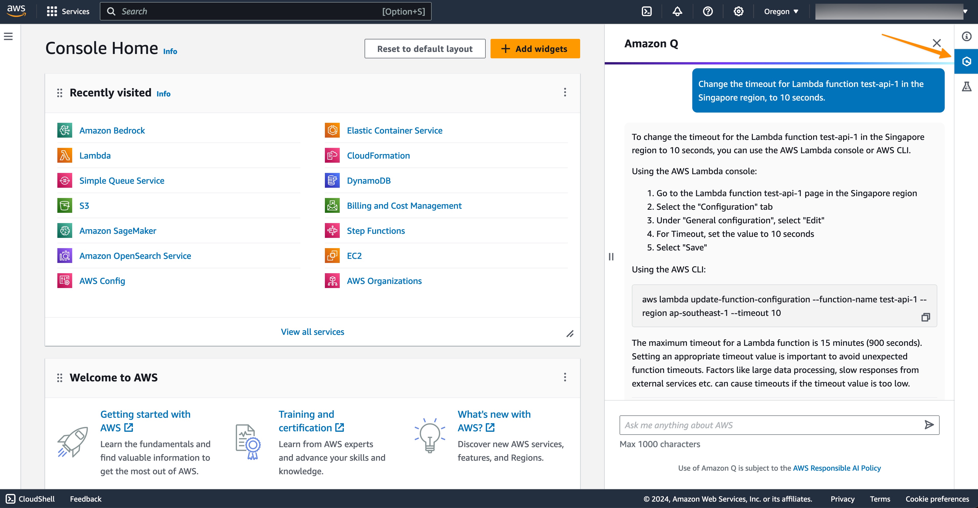
Not only that, this capability can also generate AWS Command Line Interface (AWS CLI) commands so I can make changes immediately. Here, I ask Amazon Q Developer to change the timeout configuration for my Lambda function.
Prompt for you to try: Change the timeout for Lambda function <NAME of AWS LAMBDA FUNCTION> in the Singapore Region to 10 seconds.
I can see Amazon Q Developer generated an AWS CLI command for me to perform the action. Next, I can copy and paste the command into my terminal to perform the change.
What I really like about this capability is that it minimizes the time and effort needed to get my account information in the AWS Management Console and generate AWS CLI commands so I can immediately implement any changes that I need. This helps me focus on my workflow to manage my AWS resources.
Amazon Q Developer can now help you understand your costs (preview) To fully maximize the value of cloud spend, I need to have a thorough understanding of my cloud costs. With this capability, I can get answers to AWS cost-related questions using natural language. This capability works by retrieving and analyzing cost data from AWS Cost Explorer.
Recently, I’ve been building a generative AI demo using Amazon SageMaker JumpStart, and this is the right timing because I need to know the total spend. So, I ask Amazon Q Developer the following prompt to know my spend in Q1 this year.
Prompt for you to try: What were the top three highest-cost services in Q1?
From the Amazon Q response, I can further investigate this result by selecting the Cost Explorer URL, which will bring me to the AWS Cost Explorer dashboard. Then, I can follow up with this prompt:
Prompt for you to try: List services in my account which have the most increment month over month. Provide details and analysis.
In short, this capability makes it easier for me to develop a deep understanding and get valuable insights into my cloud spending.
Amazon Q extension for IDEs As part of the update, we also released an Amazon Q integrated development environment (IDE) extension for Visual Studio Code and JetBrains IDEs. Now, you will see two extensions in the IDE marketplaces: (1) Amazon Q and (2) AWS Toolkit.
If you’re a new user, after installing the Amazon Q extension, you will see a sign-in page in the IDE with two options: using AWS Builder ID or single sign-on. You can continue to use Amazon Q normally.
For existing users, you will need to update the AWS Toolkit extension in your IDEs. Once you’ve finished the update, if you have existing Amazon Q and Amazon CodeWhisperer connections, even if they’re expired, the new Amazon Q extension will be automatically installed for you.
Free access for advanced capabilities in IDE As you might know, you can use AWS Builder ID to start using Amazon Q Developer in your preferred IDEs. Now, with this announcement, you have free access to two existing advanced capabilities of Amazon Q Developer in IDE, Amazon Q Developer Agent for software development and Amazon Q Developer Agent for code transformation. I’m really excited about this update!
With the Amazon Q Developer Agent for software development, Amazon Q Developer can help you develop code features for projects in your IDE. To get started, you enter /dev in the Amazon Q Developer chat panel. My colleague Séb shared with me the following screenshot when he was using this capability for his support case project. He used the following prompt to generate an implementation plan for creating a new API in AWS Lambda:
Prompt for you to try: Add an API to list all support cases. Expose this API as a new Lambda function
Amazon Q Developer then provides an initial plan and you can keep on iterating this plan until you’re sure mostly everything is covered. Then, you can accept the plan and select Insert code.
The other capability you can access using AWS Builder ID is Developer Agent for code transformation. This capability will help you in upgrading your Java applications in IntelliJ or Visual Studio Code. Danilo described this capability last year, and you can see his thorough journey in Upgrade your Java applications with Amazon Q Code Transformation (preview).
Improvements in Amazon Q Developer Agent for Code Transformation The new transformation plan provides details specific to my applications to help me understand the overall upgrade process. To get started, I enter /transform in the Amazon Q Developer chat and provide the necessary details for Amazon Q to start upgrading my java project.
In the first step, Amazon Q identifies and provides details on the Java Development Kit (JDK) version, dependencies, and related code that needs to be updated. The dependencies upgrades now include upgrading popular frameworks to their latest major versions. For example, if you’re building with Spring Boot, it now gets upgraded to version 3 as part of the Java 17 upgrade.
In this step, if Amazon Q identifies any deprecated code that Java language specifications recommend replacing, it will make those updates automatically during the upgrade. This is a new enhancement to Amazon Q capabilities and is available now.
In the third step, this capability will build and run unit tests on the upgraded code, including fixing any issues to ensure the code compilation process will run smoothly after the upgrade.
With this capability, you can upgrade Java 8 and 11 applications that are built using Apache Maven to Java version 17. To get started with the Amazon Q Developer Agent for code transformation capability, you can read and follow the steps at Upgrade language versions with Amazon Q Code Transformation. We also have sample code for you to try this capability.
Things to know
Availability — To learn more about the availability of Amazon Q Developer capabilities, please visit Amazon Q Developer FAQs page.
Pricing — Amazon Q Developer now offers two pricing tiers – Free (free), and Pro, at $19/month/user.
Free self-paced course on AWS Skill Builder — Amazon Q Introduction is a 15-minute course that provides a high-level overview of Amazon Q, a generative AI–powered assistant, and the use cases and benefits of using it. This course is part of Amazon’s AI Ready initiative to provide free AI skills training to 2 million people globally by 2025.
Visit our Amazon Q Developer Center to find deep-dive technical content and to discover how you can speed up your software development work.
Today’s blog is from Aimy Lee, Chief Operating Officer at Penang Science Cluster, part of our global partner network for Experience AI.
Artificial intelligence (AI) is transforming the world at an incredible pace, and at Penang Science Cluster, we are determined to be at the forefront of this fast-changing landscape.
The Malaysian government is actively promoting AI literacy among citizens, demonstrating a commitment to the nation’s technological advancement. This dedication is further demonstrated by the Ministry of Education’s recent announcement to introduce AI basics into the primary school curriculum, starting in 2027.
Why we chose Experience AI
At Penang Science Cluster, we firmly believe that AI is already an essential part of everybody’s future, especially for young people, for whom technologies such as search engines, AI chatbots, image generation, and facial recognition are already deeply ingrained in their daily experiences. It is vital that we equip young people with the knowledge to understand, harness, and even create AI solutions, rather than view AI with trepidation.
With this in mind, we’re excited to be one of the first of many organisations to join the Experience AI global partner network. Experience AI is a free educational programme offering cutting-edge resources on artificial intelligence and machine learning for teachers and students. Developed in collaboration between the Raspberry Pi Foundation and Google DeepMind, as a global partner we hope the programme will bring AI literacy to thousands of students across Malaysia.
Our goal is to demystify AI and highlight its potential for positive change. The Experience AI programme resonated with our mission to provide accessible and engaging resources tailored for our beneficiaries, making it a natural fit for our efforts.
Experience AI pilot: Results and student voices
At the start of this year, we ran an Experience AI pilot with 56 students to discover how the programme resonated with young people. The positive feedback we received was incredibly encouraging! Students expressed excitement and a genuine shift in their understanding of AI.
Their comments, such as discovering the fun of learning about AI and seeing how AI can lead to diverse career paths, validated the effectiveness of the programme’s approach.
One student’s changed perspective — from fearing AI to recognising its potential — underscores the importance of addressing misconceptions. Providing accessible AI education empowers students to develop a balanced and informed outlook.
“I learnt new things and it changed my mindset that AI is not going to take over the world.” – Student who took part in the Experience AI pilot
Launching Experience AI in Malaysia
The successful pilot paved the way for our official Experience AI launch in early April. Students who participated in the pilot were proud to be a part of the launch event, sharing their AI knowledge and experience with esteemed guests, including the Chief Minister of Penang, the Deputy Finance Minister of Malaysia, and the Director of the Penang State Education Department. The presence of these leaders highlights the growing recognition of the significance of AI education.
Experience AI launch event in Malaysia
Building a vibrant AI education community
Following the launch, our immediate focus has shifted to empowering teachers. With the help of the Raspberry Pi Foundation, we’ll conduct teacher workshops to equip them with the knowledge and tools to bring Experience AI into their classrooms. Collaborating with education departments in Penang, Kedah, Perlis, Perak, and Selangor will be vital in teacher recruitment and building a vibrant AI education community.
Inspiring the next generation of AI creators
Experience AI marks an exciting start to integrating AI education within Malaysia, for both students and teachers. Our hope is to inspire a generation of young people empowered to shape the future of AI — not merely as consumers of the technology, but as active creators and innovators.
We envision a future where AI education is as fundamental as mathematics education, providing students with the tools they need to thrive in an AI-driven world. The journey of AI exploration in Malaysia has only just begun, and we’re thrilled to play a part in shaping its trajectory.
If you’re interested in partnering with us to bring Experience AI to students and teachers in your country, you can register your interest here.
To provide the best experiences, we use technologies like cookies to store and/or access device information. Consenting to these technologies will allow us to process data such as browsing behavior or unique IDs on this site. Not consenting or withdrawing consent, may adversely affect certain features and functions.
Functional
Always active
The technical storage or access is strictly necessary for the legitimate purpose of enabling the use of a specific service explicitly requested by the subscriber or user, or for the sole purpose of carrying out the transmission of a communication over an electronic communications network.
Preferences
The technical storage or access is necessary for the legitimate purpose of storing preferences that are not requested by the subscriber or user.
Statistics
The technical storage or access that is used exclusively for statistical purposes.The technical storage or access that is used exclusively for anonymous statistical purposes. Without a subpoena, voluntary compliance on the part of your Internet Service Provider, or additional records from a third party, information stored or retrieved for this purpose alone cannot usually be used to identify you.
Marketing
The technical storage or access is required to create user profiles to send advertising, or to track the user on a website or across several websites for similar marketing purposes.
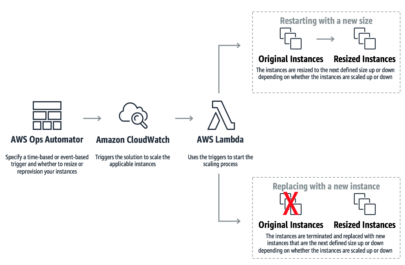

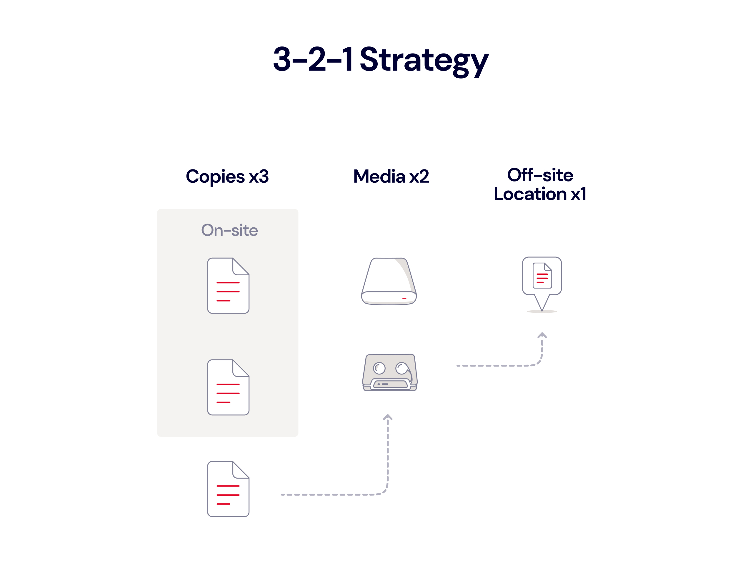
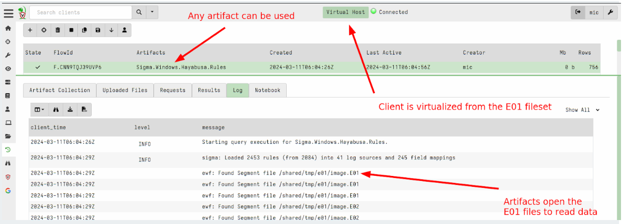
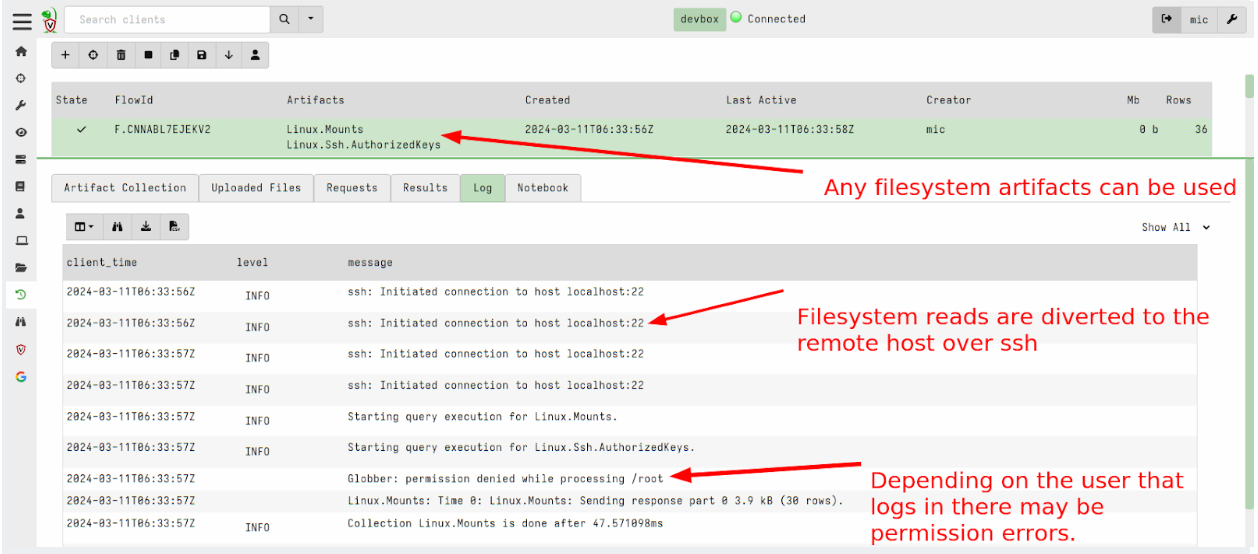
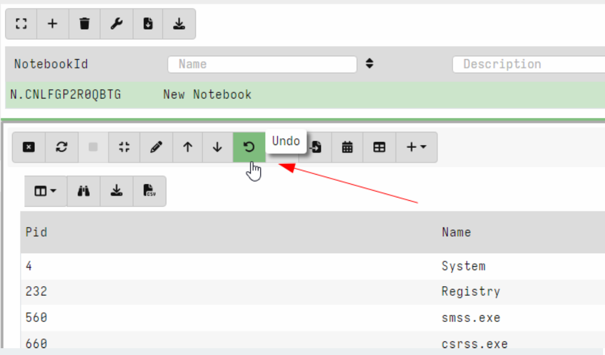
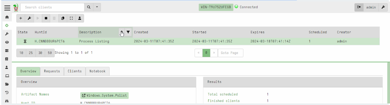
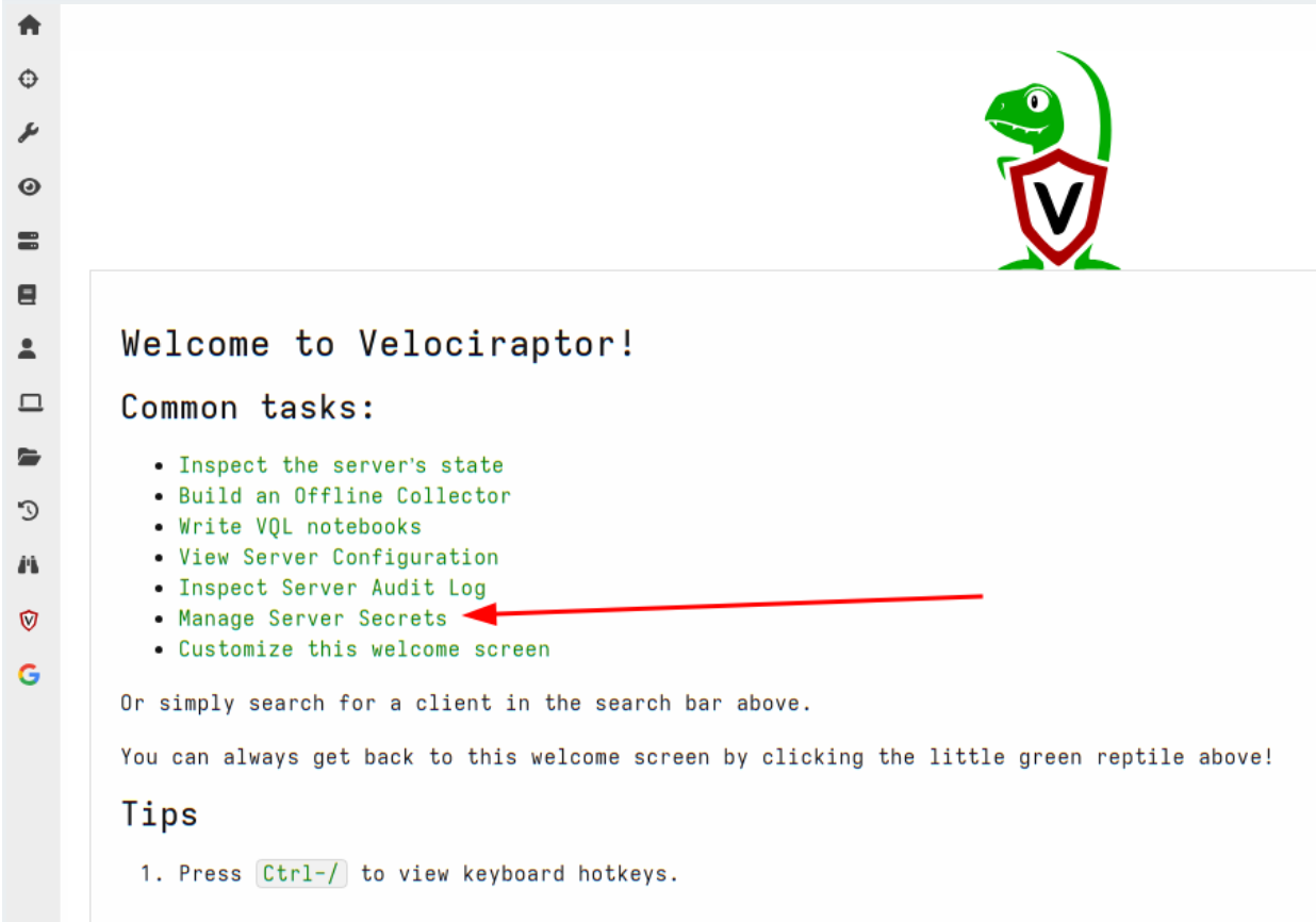
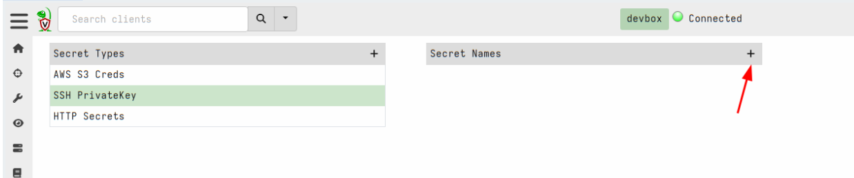
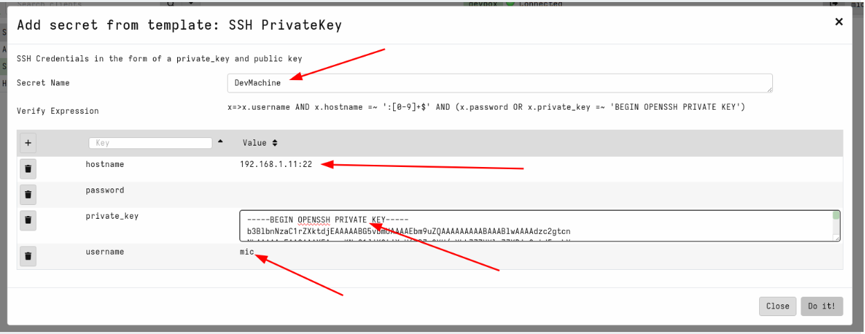
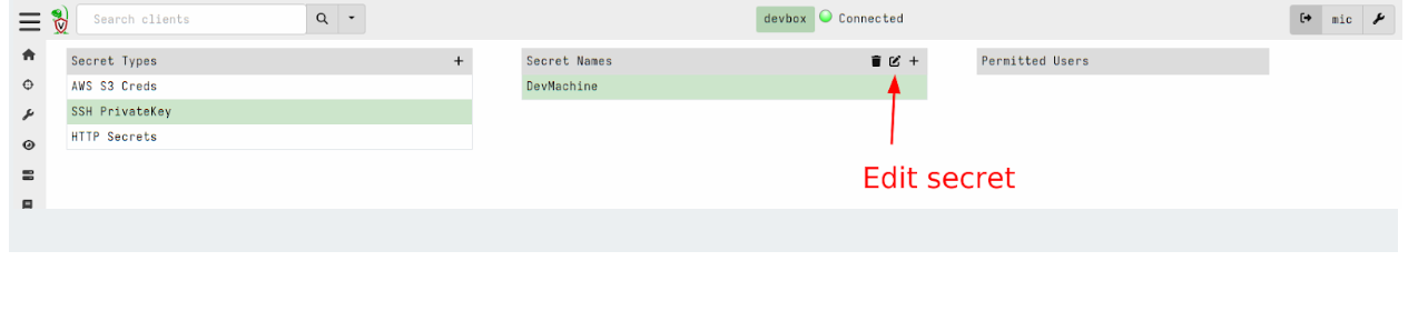
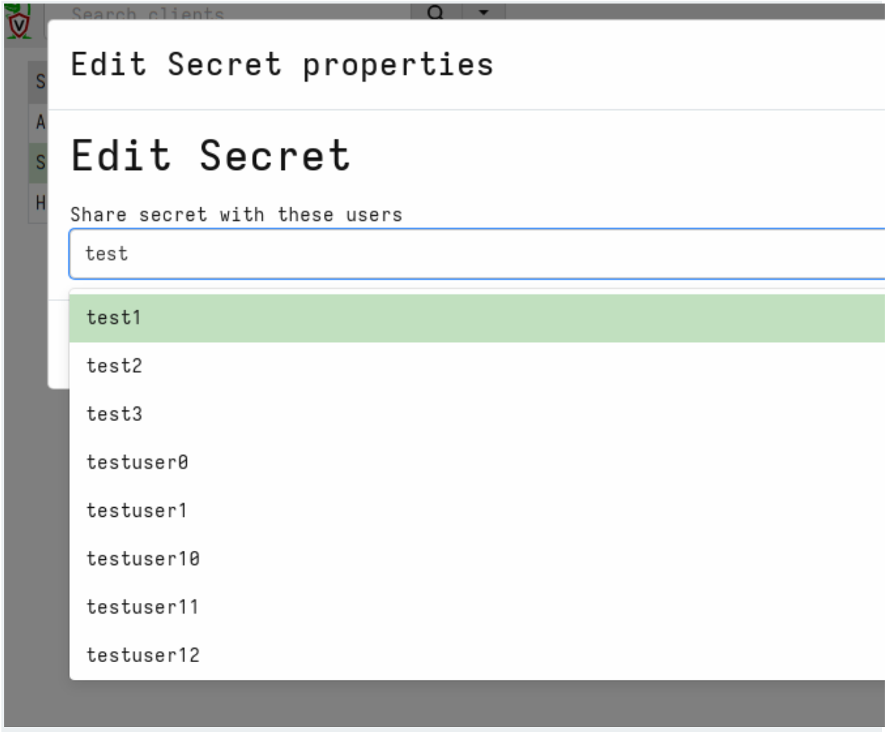
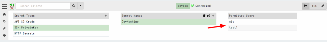
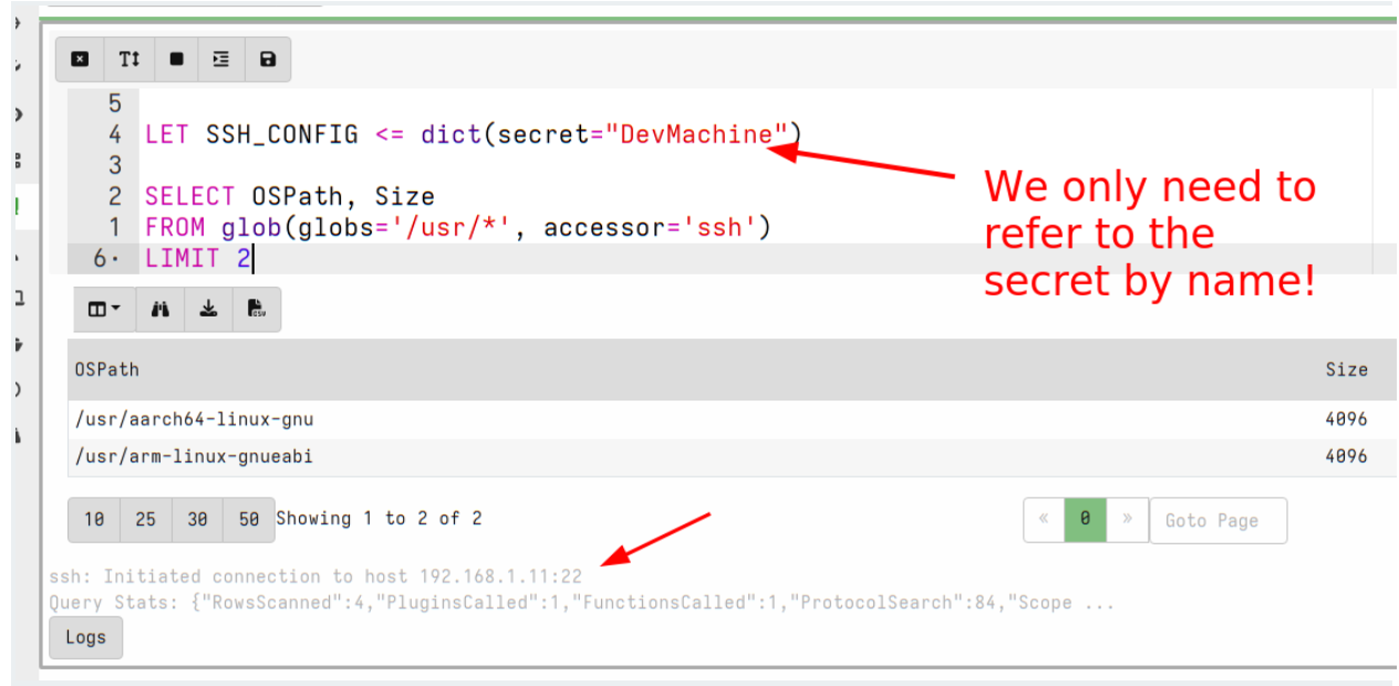
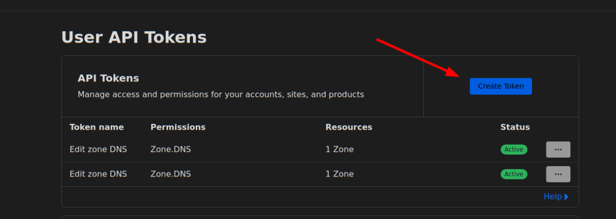
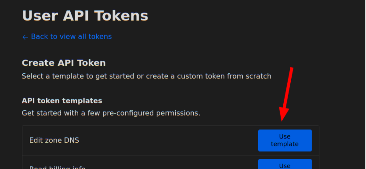
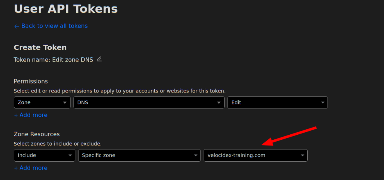


 Noritaka Sekiyama is a Principal Big Data Architect on the AWS Glue team. He is responsible for building software artifacts to help customers. In his spare time, he enjoys cycling with his road bike.
 Vishal Kajjam is a Software Development Engineer on the AWS Glue team. He is passionate about distributed computing and using ML/AI for designing and building end-to-end solutions to address customers’ data integration needs. In his spare time, he enjoys spending time with family and friends.