Backblaze Drive Stats for Q2 2023

Post Syndicated from Andy Klein original https://www.backblaze.com/blog/backblaze-drive-stats-for-q2-2023/

A decorative image with title Q2 2023 Drive Stats.

At the end of Q2 2023, Backblaze was monitoring 245,757 hard drives and SSDs in our data centers around the world. Of that number, 4,460 are boot drives, with 3,144 being SSDs and 1,316 being HDDs. The failure rates for the SSDs are analyzed in the SSD Edition: 2022 Drive Stats review.

Today, we’ll focus on the 241,297 data drives under management as we review their quarterly and lifetime failure rates as of the end of Q2 2023. Along the way, we’ll share our observations and insights on the data presented, tell you about some additional data fields we are now including and more.

Q2 2023 Hard Drive Failure Rates

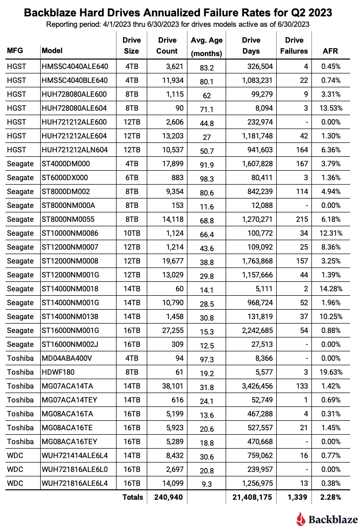
At the end of Q2 2023, we were managing 241,297 hard drives used to store data. For our review, we removed 357 drives from consideration as they were used for testing purposes or drive models which did not have at least 60 drives. This leaves us with 240,940 hard drives grouped into 31 different models. The table below reviews the annualized failure rate (AFR) for those drive models for Q2 2023.

Notes and Observations on the Q2 2023 Drive Stats

  • Zero Failures: There were six drive models with zero failures in Q2 2023 as shown in the table below.

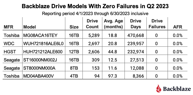
The table is sorted by the number of drive days each model accumulated during the quarter. In general a drive model should have at least 50,000 drive days in the quarter to be statistically relevant. The top three drives all meet that criteria, and having zero failures in a quarter is not surprising given the lifetime AFR for the three drives ranges from 0.13% to 0.45%. None of the bottom three drives has accumulated 50,000 drive days in the quarter, but the two Seagate drives are off to a good start. And, it is always good to see the 4TB Toshiba (model: MD04ABA400V), with eight plus years of service, post zero failures for the quarter.

  • The Oldest Drive? The drive model with the oldest average age is still the 6TB Seagate (model: ST6000DX000) at 98.3 months (8.2 years), with the oldest drive of this cohort being 104 months (8.7 years) old.

    The oldest operational data drive in the fleet is a 4TB Seagate (model: ST4000DM000) at 105.2 months (8.8 years). That is quite impressive, especially in a data center environment, but the winner for the oldest operational drive in our fleet is actually a boot drive: a WDC 500GB drive (model: WD5000BPKT) with 122 months (10.2 years) of continuous service.

  • Upward AFR: The AFR for Q2 2023 was 2.28%, up from 1.54% in Q1 2023. While quarterly AFR numbers can be volatile, they can also be useful in identifying trends which need further investigation. In this case, the rise was expected as the age of our fleet continues to increase. But was that the real reason?

    Digging in, we start with the annualized failure rates and average age of our drives grouped by drive size, as shown in the table below.

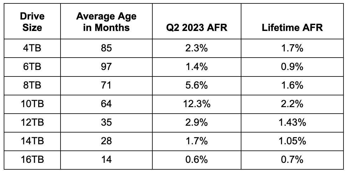
For our purpose, we’ll define a drive as old when it is five years old or more. Why? That’s the warranty period of the drives we are purchasing today. Of course, the 4TB and 6TB drives, and some of the 8TB drives, came with only two year warranties, but for consistency we’ll stick with five years as the point at which we label a drive as “old”. 

Using our definition for old drives eliminates the 12TB, 14TB and 16TB drives. This leaves us with the chart below of the Quarterly AFR over the last three years for each cohort of older drives, the 4TB, 6TB, 8TB, and 10TB models.

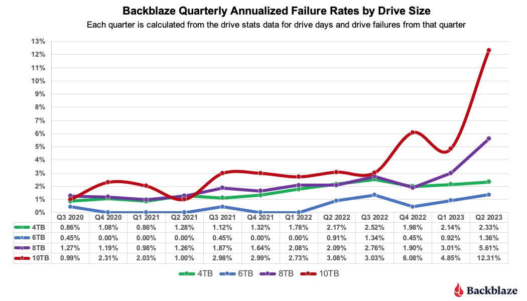
Interestingly, the oldest drives, the 4TB and 6TB drives, are holding their own. Yes, there has been an increase over the last year or so, but given their age, they are doing well.

On the other hand, the 8TB and 10TB drives, with an average of five and six years of service respectively, require further attention. We’ll look at the lifetime data later on in this report to see if our conclusions are justified.

What’s New in the Drive Stats Data?

For the past 10 years, we’ve been capturing and storing the drive stats data and since 2015 we’ve open sourced the data files that we used to create the Drive Stats reports. From time to time, new SMART attribute pairs have been added to the schema as we install new drive models which report new sets of SMART attributes. This quarter we decided to capture and store some additional data fields about the drives and the environment they operate in, and we’ve added them to the publicly available Drive Stats files that we publish each quarter. 

The New Data Fields

Beginning with the Q2 2023 Drive Stats data, there are three new data fields populated in each drive record.

  1. Vault_id: All data drives are members of a Backblaze Vault. Each vault consists of either 900 or 1,200 hard drives divided evenly across 20 storage servers.  The vault is a numeric value starting at 1,000.
  2. Pod_id: There are 20 storage servers in each Backblaze Vault. The Pod_id is a numeric field with values from 0 to 19 assigned to one of the 20 storage servers.
  3. Is_legacy_format: Currently 0, but will be useful over the coming quarters as more fields are added.

The new schema is as follows:

  • date
  • serial_number
  • model
  • capacity_bytes
  • failure
  • vault_id
  • pod_id
  • is_legacy_format
  • smart_1_normalized
  • smart_1_raw
  • Remaining SMART value pairs (as reported by each drive model)

Occasionally, our readers would ask if we had any additional information we could provide with regards to where a drive lived, and, more importantly, where it died. The newly-added data fields above are part of the internal drive data we collect each day, but they were not included in the Drive Stats data that we use to create the Drive Stats reports. With the help of David from our Infrastructure Software team, these fields will now be available in the Drive Stats data.

How Can We Use the Vault and Pod Information?

First a caveat: We have exactly one quarter’s worth of this new data. While it was tempting to create charts and tables, we want to see a couple of quarters worth of data to understand it better. Look for an initial analysis later on in the year.

That said, what this data gives us is the storage server and the vault of every drive. Working backwards, we should be able to ask questions like: “Are certain storage servers more prone to drive failure?” or, “Do certain drive models work better or worse in certain storage servers?” In addition, we hope to add data elements like storage server type and data center to the mix in order to provide additional insights into our multi-exabyte cloud storage platform.

Over the years, we have leveraged our Drive Stats data internally to improve our operational efficiency and durability. Providing these new data elements to everyone via our Drive Stats reports and data downloads is just the right thing to do.

There’s a New Drive in Town

If you do decide to download our Drive Stats data for Q2 2023, there’s a surprise inside—a new drive model. There are only four of these drives, so they’d be easy to miss, and they are not listed on any of the tables and charts we publish as they are considered “test” drives at the moment. But, if you are looking at the data, search for model “WDC WUH722222ALE6L4” and you’ll find our newly installed 22TB WDC drives. They went into testing in late Q2 and are being put through their paces as we speak. Stay tuned. (Psst, as of 7/28, none had failed.)

Lifetime Hard Drive Failure Rates

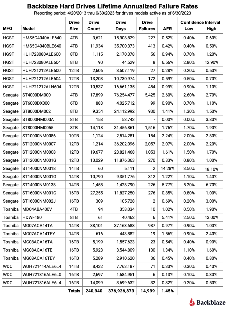
As of June 30, 2023, we were tracking 241,297 hard drives used to store customer data. For our lifetime analysis, we removed 357 drives that were only used for testing purposes or did not have at least 60 drives represented in the full dataset. This leaves us with 240,940 hard drives grouped into 31 different models to analyze for the lifetime table below.

Notes and Observations About the Lifetime Stats

The Lifetime AFR also rises. The lifetime annualized failure rate for all the drives listed above is 1.45%. That is an increase of 0.05% from the previous quarter of 1.40%. Earlier in this report by examining the Q2 2023 data, we identified the 8TB and 10TB drives as primary suspects in the increasing rate. Let’s see if we can confirm that by examining the change in the lifetime AFR rates of the different drives grouped by size.

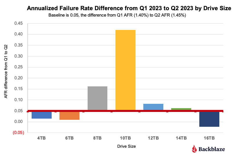
The red line is our baseline as it is the difference from Q1 to Q2 (0.05%) of the lifetime AFR for all drives. Drives above the red line support the increase, drives below the line subtract from the increase. The primary drives (by size) which are “driving” the increased lifetime annualized failure rate are the 8TB and 10TB drives. This confirms what we found earlier. Given there are relatively few 10TB drives (1,124) versus 8TB drives (24,891), let’s dig deeper into the 8TB drives models.

The Lifetime AFR for all 8TB drives jumped from 1.42% in Q1 to 1.59% in Q2.  An increase of 12%. There are six 8TB drive models in operation, but three of these models comprise 99.5% of the drive failures for the 8TB drive cohort, so we’ll focus on them. They are listed below.

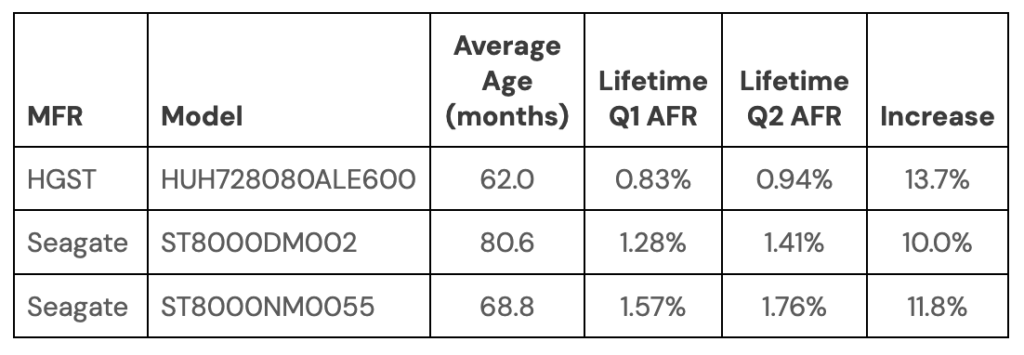
For all three models, the increase of the lifetime annualized failure rate from Q1 to Q2 is 10% or more which is statistically similar to the 12% increase for all of the 8TB drive models. If you had to select one drive model to focus on for migration, any of the three would be a good candidate. But, the Seagate drives, model ST8000DM002, are on average nearly a year older than the other drive models in question.

  • Not quite a lifetime? The table above analyzes data for the period of April 20, 2013 through June 30, 2023, or 10 years, 2 months and 10 days. As noted earlier, the oldest drive we have is 10 years and 2 months old, give or take a day or two. It would seem we need to change our table header, but not quite yet. A drive that was installed anytime in Q2 2013 and is still operational today would report drive days as part of the lifetime data for that model. Once all the drives installed in Q2 2013 are gone, we can change the start date on our tables and charts accordingly.

A Word About Drive Failure

Are we worried about the increase in drive failure rates? Of course we’d like to see them lower, but the inescapable reality of the cloud storage business is that drives fail. Over the years, we have seen a wide range of failure rates across different manufacturers, drive models, and drive sizes. If you are not prepared for that, you will fail. As part of our preparation, we use our drive stats data as one of the many inputs into understanding our environment so we can adjust when and as we need.

So, are we worried about the increase in drive failure rates? No, but we are not arrogant either. We’ll continue to monitor our systems, take action where needed, and share what we can with you along the way. 

The Hard Drive Stats Data

The complete data set used to create the information used in this review is available on our Hard Drive Stats Data webpage. You can download and use this data for free for your own purpose. All we ask are three things: 1) you cite Backblaze as the source if you use the data, 2) you accept that you are solely responsible for how you use the data, and 3) you do not sell this data to anyone; it is free.

If you want the tables and charts used in this report, you can download the .zip file from Backblaze B2 Cloud Storage which contains an MS Excel spreadsheet with a tab for each of the tables or charts..

Good luck and let us know if you find anything interesting.

The post Backblaze Drive Stats for Q2 2023 appeared first on Backblaze Blog | Cloud Storage & Cloud Backup.

The Need for Trustworthy AI

Post Syndicated from Bruce Schneier original https://www.schneier.com/blog/archives/2023/08/the-need-for-trustworthy-ai.html

If you ask Alexa, Amazon’s voice assistant AI system, whether Amazon is a monopoly, it responds by saying it doesn’t know. It doesn’t take much to make it lambaste the other tech giants, but it’s silent about its own corporate parent’s misdeeds.

When Alexa responds in this way, it’s obvious that it is putting its developer’s interests ahead of yours. Usually, though, it’s not so obvious whom an AI system is serving. To avoid being exploited by these systems, people will need to learn to approach AI skeptically. That means deliberately constructing the input you give it and thinking critically about its output.

Newer generations of AI models, with their more sophisticated and less rote responses, are making it harder to tell who benefits when they speak. Internet companies’ manipulating what you see to serve their own interests is nothing new. Google’s search results and your Facebook feed are filled with paid entries. Facebook, TikTok and others manipulate your feeds to maximize the time you spend on the platform, which means more ad views, over your well-being.

What distinguishes AI systems from these other internet services is how interactive they are, and how these interactions will increasingly become like relationships. It doesn’t take much extrapolation from today’s technologies to envision AIs that will plan trips for you, negotiate on your behalf or act as therapists and life coaches.

They are likely to be with you 24/7, know you intimately, and be able to anticipate your needs. This kind of conversational interface to the vast network of services and resources on the web is within the capabilities of existing generative AIs like ChatGPT. They are on track to become personalized digital assistants.

As a security expert and data scientist, we believe that people who come to rely on these AIs will have to trust them implicitly to navigate daily life. That means they will need to be sure the AIs aren’t secretly working for someone else. Across the internet, devices and services that seem to work for you already secretly work against you. Smart TVs spy on you. Phone apps collect and sell your data. Many apps and websites manipulate you through dark patterns, design elements that deliberately mislead, coerce or deceive website visitors. This is surveillance capitalism, and AI is shaping up to be part of it.

Quite possibly, it could be much worse with AI. For that AI digital assistant to be truly useful, it will have to really know you. Better than your phone knows you. Better than Google search knows you. Better, perhaps, than your close friends, intimate partners and therapist know you.

You have no reason to trust today’s leading generative AI tools. Leave aside the hallucinations, the made-up “facts” that GPT and other large language models produce. We expect those will be largely cleaned up as the technology improves over the next few years.

But you don’t know how the AIs are configured: how they’ve been trained, what information they’ve been given, and what instructions they’ve been commanded to follow. For example, researchers uncovered the secret rules that govern the Microsoft Bing chatbot’s behavior. They’re largely benign but can change at any time.

Many of these AIs are created and trained at enormous expense by some of the largest tech monopolies. They’re being offered to people to use free of charge, or at very low cost. These companies will need to monetize them somehow. And, as with the rest of the internet, that somehow is likely to include surveillance and manipulation.

Imagine asking your chatbot to plan your next vacation. Did it choose a particular airline or hotel chain or restaurant because it was the best for you or because its maker got a kickback from the businesses? As with paid results in Google search, newsfeed ads on Facebook and paid placements on Amazon queries, these paid influences are likely to get more surreptitious over time.

If you’re asking your chatbot for political information, are the results skewed by the politics of the corporation that owns the chatbot? Or the candidate who paid it the most money? Or even the views of the demographic of the people whose data was used in training the model? Is your AI agent secretly a double agent? Right now, there is no way to know.

We believe that people should expect more from the technology and that tech companies and AIs can become more trustworthy. The European Union’s proposed AI Act takes some important steps, requiring transparency about the data used to train AI models, mitigation for potential bias, disclosure of foreseeable risks and reporting on industry standard tests.

Most existing AIs fail to comply with this emerging European mandate, and, despite recent prodding from Senate Majority Leader Chuck Schumer, the US is far behind on such regulation.

The AIs of the future should be trustworthy. Unless and until the government delivers robust consumer protections for AI products, people will be on their own to guess at the potential risks and biases of AI, and to mitigate their worst effects on people’s experiences with them.

So when you get a travel recommendation or political information from an AI tool, approach it with the same skeptical eye you would a billboard ad or a campaign volunteer. For all its technological wizardry, the AI tool may be little more than the same.

This essay was written with Nathan Sanders, and previously appeared on The Conversation.

[$] GIL removal and the Faster CPython project

Post Syndicated from jake original https://lwn.net/Articles/939981/

The Python global interpreter lock (GIL) has long been a barrier to
increasing the performance of programs by using multiple threads—the GIL
serializes access to the interpreter’s virtual machine such that only one thread
can be executing Python code at any given time. There are other mechanisms
to provide
concurrency for the language, but the specter of the GIL—and its reality as
well—have often been cited as a major negative for Python. Back in October
2021, Sam Gross introduced
a proof-of-concept, no-GIL version of the
language
. It was met with a lot of excitement at the time, but
seemed to languish to a certain extent for more than a year; now, the Python
Steering
Council has announced its intent to accept the
no-GIL feature
. It will still be some time before it lands in a
released Python version—and there is the possibility that it all has to be
rolled back at some point—but there are several companies backing the
effort, which gives it all a good chance to succeed.

New Seventh-Generation General Purpose Amazon EC2 Instances (M7i-Flex and M7i)

Post Syndicated from Jeff Barr original https://aws.amazon.com/blogs/aws/new-seventh-generation-general-purpose-amazon-ec2-instances-m7i-flex-and-m7i/

Today we are launching Amazon Elastic Compute Cloud (Amazon EC2) M7i-Flex and M7i instances powered by custom 4th generation Intel Xeon Scalable processors available only on AWS, that offer the best performance among comparable Intel processors in the cloud – up to 15% faster than Intel processors utilized by other cloud providers. M7i-Flex instances are available in the five most common sizes, and are designed to give you up to 19% better price/performance than M6i instances for many workloads. The M7i instances are available in nine sizes (with two size of bare metal instances in the works), and offer 15% better price/performance than the previous generation of Intel-powered instances.

M7i-Flex Instances
The M7i-Flex instances are a lower-cost variant of the M7i instances, with 5% better price/performance and 5% lower prices. They are great for applications that don’t fully utilize all compute resources. The M7i-Flex instances deliver a baseline of 40% CPU performance, and can scale up to full CPU performance 95% of the time. M7i-Flex instances are ideal for running general purpose workloads such as web and application servers, virtual desktops, batch processing, micro-services, databases and enterprise applications. If you are currently using earlier generations of general-purposes instances, you can adopt M7i-Flex instances without having to make changes to your application or your workload.

Here are the specs for the M7i-Flex instances:

Instance Name vCPUs
Memory
Network Bandwidth
EBS Bandwidth
m7i-flex.large 2 8 GiB up to 12.5 Gbps up to 10 Gbps
m7i-flex.xlarge 4 16 GiB up to 12.5 Gbps up to 10 Gbps
m7i-flex.2xlarge 8 32 GiB up to 12.5 Gbps up to 10 Gbps
m7i-flex.4xlarge 16 64 GiB up to 12.5 Gbps up to 10 Gbps
m7i-flex.8xlarge 32 128 GiB up to 12.5 Gbps up to 10 Gbps

M7i Instances
For workloads such as large application servers and databases, gaming servers, CPU based machine learning, and video streaming that need the largest instance sizes or high CPU continuously, you can get price/performance benefits by using M7i instances.

Here are the specs for the M7i instances:

Instance Name vCPUs
Memory
Network Bandwidth
EBS Bandwidth
m7i.large 2 8 GiB up to 12.5 Gbps up to 10 Gbps
m7i.xlarge 4 16 GiB up to 12.5 Gbps up to 10 Gbps
m7i.2xlarge 8 32 GiB up to 12.5 Gbps up to 10 Gbps
m7i.4xlarge 16 64 GiB up to 12.5 Gbps up to 10 Gbps
m7i.8xlarge 32 128 GiB 12.5 Gbps 10 Gbps
m7i.12xlarge 48 192 GiB 18.75 Gbps 15 Gbps
m7i.16xlarge 64 256 GiB 25.0 Gbps 20 Gbps
m7i.24xlarge 96 384 GiB 37.5 Gbps 30 Gbps
m7i.48xlarge 192 768 GiB 50 Gbps 40 Gbps

You can attach up to 128 EBS volumes to each M7i instance; by way of comparison, the M6i instances allow you to attach up to 28 volumes.

We are also getting ready to launch two sizes of bare metal M7i instances:

Instance Name vCPUs
Memory
Network Bandwidth
EBS Bandwidth
m7i.metal-24xl 96 384 GiB 37.5 Gbps 30 Gbps
m7i.metal-48xl 192 768 GiB 50.0 Gbps 40 Gbps

Built-In Accelerators
The Sapphire Rapids processors include four built-in accelerators, each providing hardware acceleration for a specific workload:

  • Advanced Matrix Extensions (AMX) – This set of extensions to the x86 instruction set improve deep learning and inferencing, and support workloads such as natural language processing, recommendation systems, and image recognition. The extensions provide high-speed multiplication operations on 2-dimensional matrices of INT8 or BF16 values. To learn more, read Chapter 3 of the Intel AMX Instruction Set Reference.
  • Intel Data Streaming Accelerator (DSA) – This accelerator drives high performance for storage, networking, and data-intensive workloads by offloading common data movement tasks between CPU, memory, caches, network devices, and storage devices, improving streaming data movement and transformation operations. Read Introducing the Intel Data Streaming Accelerator (Intel DSA) to learn more.
  • Intel In-Memory Analytics Accelerator (IAA) – This accelerator runs database and analytic workloads faster, with the potential for greater power efficiency. In-memory compression, decompression, and encryption at very high throughput, and a suite of analytics primitives support in-memory databases, open source database, and data stores like RocksDB and ClickHouse. To learn more, read the Intel In-Memory Analytics Accelerator (Intel IAA) Architecture Specification.
  • Intel QuickAssist Technology (QAT) -This accelerator offloads encryption, decryption, and compression, freeing up processor cores and reducing power consumption. It also supports merged compression and encryption in a single data flow. To learn more start at the Intel QuickAssist Technology (Intel QAT) Overview.

Some of these accelerators require the use of specific kernel versions, drivers, and/or compilers.

The Advanced Matrix Extensions are available on all sizes of M7i and M7i-Flex instances. The Intel QAT, Intel IAA, and Intel DSA accelerators will be available on the m7i.metal-24xl and m7i.metal-48xl instances.

Details
Here are a couple of things to keep in mind about the M7i-Flex and M7i instances:

Regions – The new instances are available in the US East (Ohio, N. Virginia), US West (Oregon), and Europe (Ireland) AWS Regions, and we plan to expand to additional regions throughout the rest of 2023.

Purchasing Options – M7i-Flex amd M7i instances are available in On-Demand, Reserved Instance, Savings Plan, and Spot form. M7i instances are also available in Dedicated Host and Dedicated Instance form.

Jeff;

За българската и немската потребителска кошница

Post Syndicated from Боян Юруков original https://yurukov.net/blog/2023/einkaufswagen/

Тази вечер имаше репортаж по bTV Новините за цените, здравословното хранене и потребителската кошница. Сравняваха с Германия. Наскоро имах два разговора точно по тази тема и затова се заслушах. Изкараха около 300 лв на човек разход за здравословно хранене в България срещу 380 лв. в Германия. Имам четири забележки към репортажа и все за неща, с които подвеждат зрителите си.

Първо, говориха за здравословно хранене повече като реклама на определени стоки, отколкото като разнообразна диета. Вкарването на прескъпи „био“ продукти в темата беше повече от излишно. Огромен проблем на здравето ни е не само липсата на движение и спорт масово заместена с пушене, но и еднообразната храна с премного кебапчета, пържено и бира и твърде малко плодове и зеленчуци. И не, салатата покрай бирата не се брои.

Второ, взимаха цените от неназован интернет магазин за доставка на храна и … Фантастико. Харесвам Фантастико, но там цените са често 30% отгоре на тези в други магазини. Същото важи за сайтовете за доставка, макар и по други причини. Затова не може да се каже, че който и да е от източниците им беше представителен за това, което плащаме.

Трето, в Германия може да се храни човек относително по-евтино от България. Ще последва едно „обаче“ след малко, но фактите са, че с ниското ДДС за храните с чисто социална насоченост, големият пазар, работещата дотация на ключови за немското земеделие и животновъдство сектори и в голяма степен наложената от държавната машина практическа липса на печалба у същите компании държащи големите вериги у нас, цените на някои продукти и марки са по-ниски. Комбинирано със значително по-високата средна заплата това означава, че е възможно разходите на човек да са по-ниски не само като процент от бюджета, но и в абсолютна стойност.

Не на последно място обаче, също толкова вярно е, че много вероятно е за вас специално това да не важи. Това казвам често когато се отвори темата – да, може да се храниш по-евтино, но ти точно няма. Причината е многопластова и първата улика е в самия репортаж на bTV – сред главните примери за здравословното хранене бяха домати, краставици и яйца. Да, има по-евтини яйца в Германия, но ако искаш всъщност да имат някакъв вкус и жълтъкът да е жълт, ще платиш 3 пъти отгоре на скъпите във Фантастико. Доматите и краставиците са далеч по-сложни. В Германия трябва бая да се търси, за да намериш нещо с някакъв вкус. При турците е по-скоро добре, но не винаги. Аз плащах по 7 евро килото за домати, които що-годе ставаха, когато в България бяха по 3 лева. Някои свикват след години и не им е такъв проблем – въпрос на приоритети.

Втората улика отново се виждаше в репортажа – сиренето. Към него може да се добави лютеница, баница и прочие. Все неща, с които сте израснали и ще търсите. Намират се по български магазини и са значително по-скъпи от България. В зависимост колко пазарувате там това би било перо в бюджета, което не е за пренебрегване.

Трети и основен фактор е хранителната култура. В България обичаме храната и вкуса ѝ. Немската потребителска кошница е различна от българската по много отношения, особено в липсата на вкус. Имах колеги немци със сходни възможности като моите, които пазаруваха неща, до които от безпаричие съм прибягвал в студентските си години. Те просто не правиха разлика във вкуса. Тук дори не включвам храненето навън или традиционната им вечеря със хляб и шунка. Гледали са ме като луд излизайки с копър, три кила краставици и две кила кисело мляко от магазина. Да напълните количката си с нещата, с които сте свикнали да се храните в България с дори близък вкус и качество ще се охарчите значително повече от онова, което bTV съобщава.

Всичко това е строго индивидуално спрямо това как се храните, какви пари получавате в България и бихте получавали в Германия, както и на какви жертви сте готови. Някои хора свикват, на други не им е проблем изначално, а на трети им харесва дори повече. За 17 години съм минал през широк спектър на възможности и съображения за храненето си. В последните 8 следя в таблица всичките си разходи. Прецених, че ще е полезно да следя изкъсо финансите си, а и исках да видя как се променят през времето спрямо инфлацията. Затова знам точно колко съм давал за храна и каква част от бюджета ми е било към всеки момент.

Продължих да го правя след като се върнах в България на този ден преди точно три години. За това време видях, че разходите ми за храна намаляха между три и четири пъти. Храним се по същия начин, в повечето случаи дори със същите продукти. Сирене, лютеница и киселото мляко ни излизат по-евтино, но шоколадът, телешкото и алкохолът са значително по-скъпи. При други хора, с които сме си споделяли по темата, разликата би била по-скоро между 80% и два пъти, което отново е значително. Всичко зависи от навиците и за какво решиш да даваш пари.

Затова когато видите следващия път снимки на разминаващи се цени в български и немски, холандски, британски или където и да е там магазини, замислете се дали не е поредната въдица за кликове караща ви да гледате през ключалка нещо изолирано и крайно конкретно. Също, ако наистина сте решени да заминете за друга държава, приемете, че ще трябва значително да промените доста повече от езика и пощенския си код. Може би това е целта ви и е добра цел стига да е добре осъзната.

The post За българската и немската потребителска кошница first appeared on Блогът на Юруков.

Automatically delete schedules upon completion with Amazon EventBridge Scheduler

Post Syndicated from Marcia Villalba original https://aws.amazon.com/blogs/compute/automatically-delete-schedules-upon-completion-with-amazon-eventbridge-scheduler/

Amazon EventBridge Scheduler now supports configuring automatic deletion of schedules after completion. Now you can configure one-time and recurring schedules with an end date to be automatically deleted upon completion to avoid managing individual schedules.

Amazon EventBridge Scheduler allows you to create, run, and manage schedules on scale. Using EventBridge Scheduler, you can schedule millions of tasks to invoke over 270 AWS services and over 6,000 API operations, such as AWS Lambda, AWS Step Functions, and Amazon SNS.

By default, EventBridge Scheduler allows customers to have 1 million schedules per account, which can be increased as needed. However, completed schedules are counted towards the account quota limits. In addition, completed schedules are visible when listing schedules, and require customers to remove them. Some customers have created their own patterns to automatically remove completed schedules and since the EventBridge Scheduler announcement last November, this was one of the most requested features by customers.

Deleting after completion

When you configure automatic deletion for a schedule, EventBridge Scheduler deletes the schedule shortly after its last target invocation. You can set up automatic deletion when you create the schedule, or you can update the schedule settings at any point before its last invocation.

You can configure this setting in one-time and recurring schedules.

  • One-time schedules: your schedule is deleted after the schedule has invoked its target once.
  • Recurring schedules: set with rate or cron expressions, your schedule is deleted after the last invocation.

If all retries are exhausted because of failure for a schedule configured with automatic deletion, the schedule is deleted shortly after the last unsuccessful attempt.

Console action after schedule completition

With this new capability, you can save time, resources, and operational costs when managing your schedules.

Setting up schedules to delete after completion

You can create schedules that are automatically deleted after completion from the AWS Management Console, AWS SDK, or AWS CLI in all AWS Regions where EventBridge Scheduler is available.

For example, imagine that you are a developer on a platform that allows end users to receive notifications when a task is due. You are already using EventBridge Scheduler to implement this feature. For every task that your users create in your application, your code creates a new schedule in EventBridge Scheduler. You can now configure all these schedules to be deleted automatically after completion. And shortly after the schedules run, they are removed from your EventBridge Scheduler, allowing you to scale your system and keep on creating schedules, making it easier to manage your active schedules and quota limits.

Let see how you can implement this example with the new capability of EventBridge Scheduler. When a user creates a new task with a reminder, a function is triggered from your application. That function creates a one-time schedule in EventBridge Scheduler.

Create a schedule diagram

This example shows how you can create a new one-time schedule that is automatically deleted after completion using the AWS CLI and has SNS as a target. Make sure that you update the AWS CLI to the latest version. Then you can create a new schedule with the parameter action-after-completion ‘DELETE’.

$ aws scheduler create-schedule --name SendEmailOnce \
--schedule-expression ”at(2023-08-02T17:35:00)",\
--schedule-expression-timezone "Europe/Helsinki" \
--flexible-time-window "{\"Mode\": \"OFF\"}" \
--target "{\"Arn\": \"arn:aws:sns:us-east-1:xxx:test-send-email\", \"RoleArn\": \" arn:aws:iam::xxxx:role/sam_scheduler_role\" }" \
--action-after-completion 'DELETE'

This command creates a one-time schedule with the name SendEmailOnce, that runs at a specific date, defined in the schedule-expression, and in a specific time zone, defined in the schedule-expression-timezone. This schedule is not using the flexible time window feature. Next, you must define the target for this schedule. This one sends a message to an SNS topic.

You can validate that your schedule is created correctly from the AWS CLI with the get-schedule command.

$ aws scheduler get-schedule --name SendEmailOnce
{
    "ActionAfterCompletion": "DELETE",
    "Arn": "arn:aws:scheduler:us-east-1:905614108351:schedule/default/SendEmailOnce",
    "CreationDate": 1690874334.83,
    "FlexibleTimeWindow": {
        "Mode": "OFF"
    },
    "GroupName": "default",
    "LastModificationDate": 1690874334.83,
    "Name": "SendEmailOnce3",
    "ScheduleExpression": "at(2023-08-02T17:35:00)",
    "ScheduleExpressionTimezone": "Europe/Helsinki",
    "State": "ENABLED",
    "Target": {
        "Arn": "arn:aws:sns:us-east-1:xxxx:test-send-email",
        "RetryPolicy": {
            "MaximumEventAgeInSeconds": 86400,
            "MaximumRetryAttempts": 185
        },
        "RoleArn": "arn:aws:iam::XXXX:role/scheduler_role"
    }
}

In addition, you can see the details of the schedule from the AWS Management Console.

Schedule details

Now when the date of the notification arrives, EventBridge Scheduler invokes the target configured in the schedule, in this case SNS, and emails a notification to the customer.

Schedule starts

Shortly after this schedule is completed, if you list the schedules, you see that the schedule was deleted and it is no longer listed.

$ aws scheduler list-schedules
{
"Schedules": [
]
}

Benefits of automation

Traditionally, many problems that EventBridge Scheduler solves were addressed using batch processes and pull-based models.

Some organizations are using EventBridge Scheduler to replace their pull-based models for a more dynamic push-based model. Before implementing Scheduler, they were relying on the customer to ask for the data when they need it. Now, with EventBridge Scheduler, they are creating schedules to report back to their customers at critical times of their journey.

For example, an airline can use EventBridge Scheduler to create one-time schedules 24 hours, 4 hours, and 2 hours before the flight, to keep their passengers up to date with the flight status. Customers receive a notification with the link for the online check-in, the check-in counter number, baggage pick up information, and any flight changes that occur. In this way, passengers are always up to date on their flight status and they can take immediate action. This dynamic model not only helps to improve the customer experience but also improves the operational efficiency for the airline.

Other organizations use EventBridge Scheduler to replace batch operations, as you can configure a schedule that starts a batch process at the time of the day you need. Also, you can take advantage of EventBridge Scheduler time zones and run the processes at the time that make sense for your end customer.

For example, consider an international financial institution that must send customers a statement of their account at the end of the day. You can use EventBridge Scheduler to set up a recurrent schedule for each of your customers that sends a report at the end of the day of your customers’ time zone. In this way, you can improve the customer experience as now the system is personalized for their settings, and also reduce operational overhead, as the processing operations are distributed throughout the day.

In addition, EventBridge Scheduler solves many new use cases for customers. For example, if you are a financial institution that handles payments, you can create a one-time schedule for every large transaction that needs a confirmation. If the transaction is not confirmed when the schedule runs, you can cancel the transaction. This decreases the risk of handling transactions, improves the customer experience, and also improves the automation of your processes by making them real time.

Another use case is to handle credit card expiration dates. You can create a one-time schedule that emails the customer to update their credit card information one month before the expiration date. This solution removes operational overhead compared to the traditional implementation of using servers and batch processes.

Conclusion

In the preceding use cases listed, automation and task scheduling improve the end user experience, remove undifferentiated heavy lifting, and benefit from using the new capability of removing schedules after their completion.

This blog post introduces the new capability from Amazon EventBridge Scheduler that automatically deletes the completed schedules. This feature simplifies the use of EventBridge Scheduler, reduces the operational overhead of managing schedules at scale, and allows you to scale even further.

To get started with EventBridge Scheduler, visit Serverless Land patterns where you can find over 20 patterns using this service.

Estimating Scope 1 Carbon Footprint with Amazon Athena

Post Syndicated from Thomas Burns original https://aws.amazon.com/blogs/big-data/estimating-scope-1-carbon-footprint-with-amazon-athena/

Today, more than 400 organizations have signed The Climate Pledge, a commitment to reach net-zero carbon by 2040. Some of the drivers that lead to setting explicit climate goals include customer demand, current and anticipated government relations, employee demand, investor demand, and sustainability as a competitive advantage. AWS customers are increasingly interested in ways to drive sustainability actions. In this blog, we will walk through how we can apply existing enterprise data to better understand and estimate Scope 1 carbon footprint using Amazon Simple Storage Service (S3) and Amazon Athena, a serverless interactive analytics service that makes it easy to analyze data using standard SQL.

The Greenhouse Gas Protocol

The Greenhouse Gas Protocol (GHGP) provides standards for measuring and managing global warming impacts from an organization’s operations and value chain.

The greenhouse gases covered by the GHGP are the seven gases required by the UNFCCC/Kyoto Protocol (which is often called the “Kyoto Basket”). These gases are carbon dioxide (CO2), methane (CH4), nitrous oxide (N2O), the so-called F-gases (hydrofluorocarbons and perfluorocarbons), sulfur hexafluoride (SF6) nitrogen trifluoride (NF3). Each greenhouse gas is characterized by its global warming potential (GWP), which is determined by the gas’s greenhouse effect and its lifetime in the atmosphere. Since carbon dioxide (CO2) accounts for about 76 percent of total man-made greenhouse gas emissions, the global warming potential of greenhouse gases are measured relative to CO2, and are thus expressed as CO2-equivalent (CO2e).

The GHGP divides an organization’s emissions into three primary scopes:

  • Scope 1 – Direct greenhouse gas emissions (for example from burning fossil fuels)
  • Scope 2 – Indirect emissions from purchased energy (typically electricity)
  • Scope 3 – Indirect emissions from the value chain, including suppliers and customers

How do we estimate greenhouse gas emissions?

There are different methods to estimating GHG emissions that includes the Continuous Emissions Monitoring System (CEMS) Method, the Spend-Based Method, and the Consumption-Based Method.

Direct Measurement – CEMS Method

An organization can estimate its carbon footprint from stationary combustion sources by performing a direct measurement of carbon emissions using the CEMS method. This method requires continuously measuring the pollutants emitted in exhaust gases from each emissions source using equipment such as gas analyzers, gas samplers, gas conditioning equipment (to remove particulate matter, water vapor and other contaminants), plumbing, actuated valves, Programmable Logic Controllers (PLCs) and other controlling software and hardware. Although this approach may yield useful results, CEMS requires specific sensing equipment for each greenhouse gas to be measured, requires supporting hardware and software, and is typically more suitable for Environment Health and Safety applications of centralized emission sources. More information on CEMS is available here.

Spend-Based Method

Because the financial accounting function is mature and often already audited, many organizations choose to use financial controls as a foundation for their carbon footprint accounting. The Economic Input-Output Life Cycle Assessment (EIO LCA) method is a spend-based method that combines expenditure data with monetary-based emission factors to estimate the emissions produced. The emission factors are published by the U.S. Environment Protection Agency (EPA) and other peer-reviewed academic and government sources. With this method, you can multiply the amount of money spent on a business activity by the emission factor to produce the estimated carbon footprint of the activity.

For example, you can convert the amount your company spends on truck transport to estimated kilograms (KG) of carbon dioxide equivalent (CO₂e) emitted as shown below.

Estimated Carbon Footprint = Amount of money spent on truck transport * Emission Factor [1]

Although these computations are very easy to make from general ledgers or other financial records, they are most valuable for initial estimates or for reporting minor sources of greenhouse gases. As the only user-provided input is the amount spent on an activity, EIO LCA methods aren’t useful for modeling improved efficiency. This is because the only way to reduce EIO-calculated emissions is to reduce spending. Therefore, as a company continues to improve its carbon footprint efficiency, other methods of estimating carbon footprint are often more desirable.

Consumption-Based Method

From either Enterprise Resource Planning (ERP) systems or electronic copies of fuel bills, it’s straightforward to determine the amount of fuel an organization procures during a reporting period. Fuel-based emission factors are available from a variety of sources such as the US Environmental Protection Agency and commercially-licensed databases. Multiplying the amount of fuel procured by the emission factor yields an estimate of the CO2e emitted through combustion. This method is often used for estimating the carbon footprint of stationary emissions (for instance backup generators for data centers or fossil fuel ovens for industrial processes).

If for a particular month an enterprise consumed a known amount of motor gasoline for stationary combustion, the Scope 1 CO2e footprint of the stationary gasoline combustion can be estimated in the following manner:

Estimated Carbon Footprint = Amount of Fuel Consumed * Stationary Combustion Emission Factor[2]

Organizations may estimate their carbon emissions by using existing data found in fuel and electricity bills, ERP data, and relevant emissions factors, which are then consolidated in to a data lake. Using existing analytics tools such as Amazon Athena and Amazon QuickSight an organization can gain insight into its estimated carbon footprint.

The data architecture diagram below shows an example of how you could use AWS services to calculate and visualize an organization’s estimated carbon footprint.

Analytics Architecture

Customers have the flexibility to choose the services in each stage of the data pipeline based on their use case. For example, in the data ingestion phase, depending on the existing data requirements, there are many options to ingest data into the data lake such as using the AWS Command Line Interface (CLI), AWS DataSync, or AWS Database Migration Service.

Example of calculating a Scope 1 stationary emissions footprint with AWS services

Let’s assume you burned 100 standard cubic feet (scf) of natural gas in an oven. Using the US EPA emission factors for stationary emissions we can estimate the carbon footprint associated with the burning. In this case the emission factor is 0.05449555 Kg CO2e /scf.[3]

Amazon S3 is ideal for building a data lake on AWS to store disparate data sources in a single repository, due to its virtually unlimited scalability and high durability. Athena, a serverless interactive query service, allows the analysis of data directly from Amazon S3 using standard SQL without having to load the data into Athena or run complex extract, transform, and load (ETL) processes. Amazon QuickSight supports creating visualizations of different data sources, including Amazon S3 and Athena, and the flexibility to use custom SQL to extract a subset of the data. QuickSight dashboards can provide you with insights (such as your company’s estimated carbon footprint) quickly, and also provide the ability to generate standardized reports for your business and sustainability users.

In this example, the sample data is stored in a file system and uploaded to Amazon S3 using the AWS Command Line Interface (CLI) as shown in the following architecture diagram. AWS recommends creating AWS resources and managing CLI access in accordance with the Best Practices for Security, Identity, & Compliance guidance.

The AWS CLI command below demonstrates how to upload the sample data folders into the S3 target location.

aws s3 cp /path/to/local/file s3://bucket-name/path/to/destination

The snapshot of the S3 console shows two newly added folders that contains the files.

S3 Bucket Overview of Files

To create new table schemas, we start by running the following script for the gas utilization table in the Athena query editor using Hive DDL. The script defines the data format, column details, table properties, and the location of the data in S3.

CREATE EXTERNAL TABLE `gasutilization`(
`fuel_id` int,
`month` string,
`year` int,
`usage_therms` float,
`usage_scf` float,
`g-nr1_schedule_charge` float,
`accountfee` float,
`gas_ppps` float,
`netcharge` float,
`taxpercentage` float,
`totalcharge` float)
ROW FORMAT DELIMITED
FIELDS TERMINATED BY ','
STORED AS INPUTFORMAT
'org.apache.hadoop.mapred.TextInputFormat'
OUTPUTFORMAT
'org.apache.hadoop.hive.ql.io.HiveIgnoreKeyTextOutputFormat'
LOCATION
's3://<bucketname>/Scope 1 Sample Data/gasutilization'
TBLPROPERTIES (
'classification'='csv',
'skip.header.line.count'='1')

Athena Hive DDLThe script below shows another example of using Hive DDL to generate the table schema for the gas emission factor data.

CREATE EXTERNAL TABLE `gas_emission_factor`(
`fuel_id` int,
`gas_name` string,
`emission_factor` float)
ROW FORMAT DELIMITED
FIELDS TERMINATED BY ','
STORED AS INPUTFORMAT
'org.apache.hadoop.mapred.TextInputFormat'
OUTPUTFORMAT
'org.apache.hadoop.hive.ql.io.HiveIgnoreKeyTextOutputFormat'
LOCATION
's3://<bucketname>/Scope 1 Sample Data/gas_emission_factor'
TBLPROPERTIES (
'classification'='csv',
'skip.header.line.count'='1')

After creating the table schema in Athena, we run the below query against the gas utilization table that includes details of gas bills to show the gas utilization and the associated charges, such as gas public purpose program surcharge (PPPS) and total charges after taxes for the year of 2020:

SELECT * FROM "gasutilization" where year = 2020;

Athena gas utilization overview by month

We are also able to analyze the emission factor data showing the different fuel types and their corresponding CO2e emission as shown in the screenshot.

athena co2e emission factor

With the emission factor and the gas utilization data, we can run the following query below to get an estimated Scope 1 carbon footprint alongside other details. In this query, we joined the gas utilization table and the gas emission factor table on fuel id and multiplied the gas usage in standard cubic foot (scf) by the emission factor to get the estimated CO2e impact. We also selected the month, year, total charge, and gas usage measured in therms and scf, as these are often attributes that are of interest for customers.

SELECT "gasutilization"."usage_scf" * "gas_emission_factor"."emission_factor" 
AS "estimated_CO2e_impact", 
"gasutilization"."month", 
"gasutilization"."year", 
"gasutilization"."totalcharge", 
"gasutilization"."usage_therms", 
"gasutilization"."usage_scf" 
FROM "gasutilization" 
JOIN "gas_emission_factor" 
on "gasutilization"."fuel_id"="gas_emission_factor"."fuel_id";

athena join

Lastly, Amazon QuickSight allows visualization of different data sources, including Amazon S3 and Athena, and the flexibility to use custom SQL to get a subset of the data. The following is an example of a QuickSight dashboard showing the gas utilization, gas charges, and estimated carbon footprint across different years.

QuickSight sample dashboard

We have just estimated the Scope 1 carbon footprint for one source of stationary combustion. If we were to do the same process for all sources of stationary and mobile emissions (with different emissions factors) and add the results together, we could roll up an accurate estimate of our Scope 1 carbon emissions for the entire business by only utilizing native AWS services and our own data. A similar process will yield an estimate of Scope 2 emissions, with grid carbon intensity in the place of Scope 1 emission factors.

Summary

This blog discusses how organizations can use existing data in disparate sources to build a data architecture to gain better visibility into Scope 1 greenhouse gas emissions. With Athena, S3, and QuickSight, organizations can now estimate their stationary emissions carbon footprint in a repeatable way by applying the consumption-based method to convert fuel utilization into an estimated carbon footprint.

Other approaches available on AWS include Carbon Accounting on AWS, Sustainability Insights Framework, Carbon Data Lake on AWS, and general guidance detailed at the AWS Carbon Accounting Page.

If you are interested in information on estimating your organization’s carbon footprint with AWS, please reach out to your AWS account team and check out AWS Sustainability Solutions.

References

  1. An example from page four of Amazon’s Carbon Methodology document illustrates this concept.
    Amount spent on truck transport: $100,000
    EPA Emission Factor: 1.556 KG CO2e /dollar of truck transport
    Estimated CO₂e emission: $100,000 * 1.556 KG CO₂e/dollar of truck transport = 155,600 KG of CO2e
  2. For example,
    Gasoline consumed: 1,000 US Gallons
    EPA Emission Factor: 8.81 Kg of CO2e /gallon of gasoline combusted
    Estimated CO2e emission = 1,000 US Gallons * 8.81 Kg of CO2e per gallon of gasoline consumed= 8,810 Kg of CO2e.
    EPA Emissions Factor for stationary emissions of motor gasoline is 8.78 kg CO2 plus .38 grams of CH4, plus .08 g of N2O.
    Combining these emission factors using 100-year global warming potential for each gas (CH4:25 and N2O:298) gives us Combined Emission Factor = 8.78 kg + 25*.00038 kg + 298 *.00008 kg = 8.81 kg of CO2e per gallon.
  3. The Emission factor per scf is 0.05444 kg of CO2 plus 0.00103 g of CH4 plus 0.0001 g of N2O. To get this in terms of CO2e we need to multiply the emission factor of the other two gases by their global warming potentials (GWP). The 100-year GWP for CH4  and N2O are 25 and 298 respectively. Emission factors and GWPs come from the US EPA website.


About the Authors


Thomas Burns
, SCR, CISSP is a Principal Sustainability Strategist and Principal Solutions Architect at Amazon Web Services. Thomas supports manufacturing and industrial customers world-wide. Thomas’s focus is using the cloud to help companies reduce their environmental impact both inside and outside of IT.

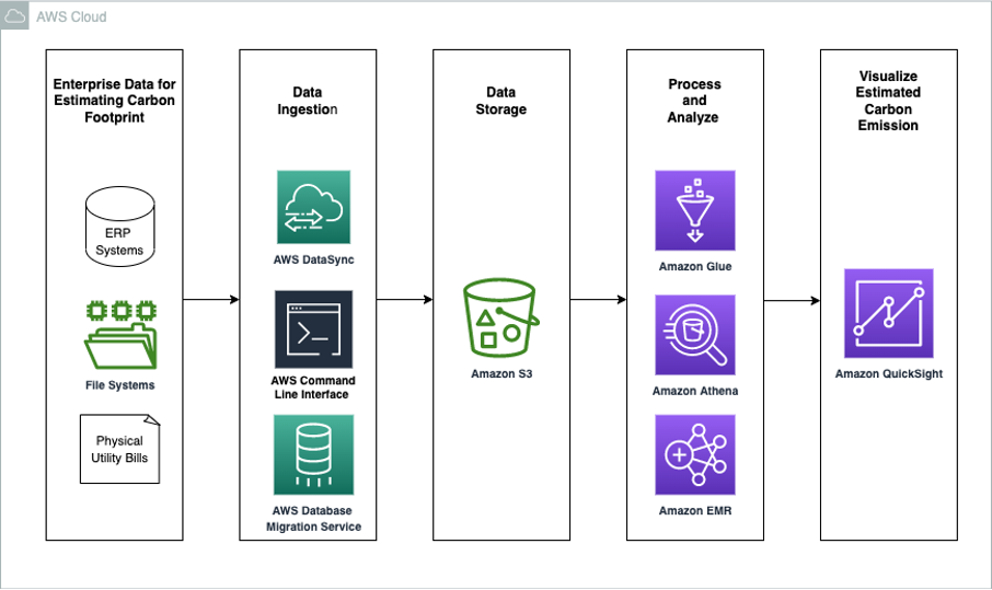
Aileen Zheng is a Solutions Architect supporting US Federal Civilian Sciences customers at Amazon Web Services (AWS). She partners with customers to provide technical guidance on enterprise cloud adoption and strategy and helps with building well-architected solutions. She is also very passionate about data analytics and machine learning. In her free time, you’ll find Aileen doing pilates, taking her dog Mumu out for a hike, or hunting down another good spot for food! You’ll also see her contributing to projects to support diversity and women in technology.

Poorly Purged Medical Devices Present Security Concerns After Sale on Secondary Market

Post Syndicated from Deral Heiland original https://blog.rapid7.com/2023/08/02/security-implications-improper-deacquisition-medical-infusion-pumps/

Poorly Purged Medical Devices Present Security Concerns After Sale on Secondary Market

In a post-pandemic landscape, the interconnectedness of cybersecurity is front and center. Few could say that they were not at least aware of, if not directly affected by, the downstream effects of major breaches that cause impacts felt across economies. One should look at disruptions in the global supply chain as case in point.

So the concept of security that goes from the cradle to the grave, is more than just an industry buzz phrase, it is a critical component of securing networks, applications, and devices.

Sadly, in too many cases, cradle to grave security was either not considered at conception, or outright ignored. And as a new report released today by Rapid7 principal researcher, Deral Heiland points out, even when organizations are able to take steps to mitigate concerns at the grave portion of the life cycle, they don’t.

In Security Implications from Improper De-acquisition of Medical Infusion Pumps Heiland performs a physical and technical teardown of more than a dozen medical infusion pumps — devices used to deliver and control fluids directly into a patient’s body. Each of these devices was available for purchase on the secondary market and each one had issues that could compromise their previous organization’s networks.

The reason these devices pose such a risk is a lack of (or lax) process for de-acquisitioning them before they are sold on sites like eBay. In at least eight of the 13 devices used in the study, WiFi PSK access credentials were discovered, offering attackers potential access to health organization networks.

In the report, Heiland calls for systemic changes to policies and procedures for both the acquisition and de-acquisition of these devices. The policies must define ownership and governance of these devices from the moment they enter the building to the moment they are sold on the secondary market. The processes should detail how data should be purged from these devices (and by extension, many others). In the cases of medical devices that are leased, contractual agreements on the purging process and expectations should be made before acquisition.

The ultimate finding is that properly disposing of sensitive information on these devices should be a priority. Purging them of data should not (and in many cases is not) terribly difficult. The issue lies with process and responsibility for the protection of information stored in those devices. And that is a major component of the cradle to grave security concept.

If you would like to read the report it is available here.

Project Zero on Arm MTE

Post Syndicated from corbet original https://lwn.net/Articles/940152/

Google’s Project Zero has spent some time studying the Arm memory tagging
extension (MTE), support for which was
merged into the 5.10 kernel, and posted
the results
:

Despite its limitations, MTE is still by far the most promising
path forward for improving C/C++ software security in 2023. The
ability of MTE to detect memory corruption exploitation at the
first dangerous access provides a significant improvement in
diagnostic and potential security effectiveness.

There is a
separate section
on weaknesses in the current kernel implementation of
MTE support.

DapuStor Haishen5 HS5100 PCIe Gen5 NVMe SSD with Marvell Bravera in Production

Post Syndicated from Cliff Robinson original https://www.servethehome.com/dapustor-haishen5-hs5100-pcie-gen5-nvme-ssd-with-marvell-bravera-in-production-kioxia/

The DapuStor Haishen5 HS5100 is a new PCIe Gen5 NVMe SSD, based on a Marvell Bravera SC5 controller, that has now entered mass production

The post DapuStor Haishen5 HS5100 PCIe Gen5 NVMe SSD with Marvell Bravera in Production appeared first on ServeTheHome.

How FIS ingests and searches vector data for quick ticket resolution with Amazon OpenSearch Service

Post Syndicated from Rupesh Tiwari original https://aws.amazon.com/blogs/big-data/how-fis-ingests-and-searches-vector-data-for-quick-ticket-resolution-with-amazon-opensearch-service/

This post was co-written by Sheel Saket, Senior Data Science Manager at FIS, and Rupesh Tiwari, Senior Architect at Amazon Web Services.

Do you ever find yourself grappling with multiple defect logging mechanisms, scattered project management tools, and fragmented software development platforms? Have you experienced the frustration of lacking a unified view, hindering your ability to efficiently manage and identify common trending issues within your enterprise? Are you constantly facing challenges when it comes to addressing defects and their impact, causing disruptions in your production cycles?

If these questions resonate with you, then you’re not alone. FIS, a leading technology and services provider, has encountered these very challenges. In their quest for a solution, they teamed up with AWS to tackle these obstacles head-on. In this post, we take you on a journey through their collaborative project, exploring how they used Amazon OpenSearch Service to transform their operations, enhance efficiency, and gain valuable insights.

This post shares FIS’s journey in overcoming challenges and provides step-by-step instructions for provisioning the solution architecture in your AWS account. You’ll learn how to implement a transformative solution that empowers your organization with near-real-time data indexing and visualization capabilities.

In the following sections, we dive into the details of FIS’s journey and discover how they overcame these challenges, revolutionizing their approach to defect management and software development.

Challenges for near-real-time ticket visualization and search

FIS faced several challenges in achieving near-real-time ticket visualization and search capabilities, including the
following:

  • Integrating ticket data from tens of different third-party systems
  • Overcoming API call thresholds and limitations from various systems
  • Implementing an efficient KNN vector search algorithm for resolving issues and performing trend analysis
  • Establishing a robust data ingestion and indexing process for real-time updates from 15,000 tickets per day
  • Ensuring unified access to ticket information across 20 development teams
  • Providing secure and scalable access to ticket data for up to 250 teams

Despite these challenges, FIS successfully enhanced their operational efficiency, enabled quick ticket resolution, and gained valuable insights through the integration of OpenSearch Service.

Let’s delve into the technical walkthrough of the architecture diagram and mechanisms. The following section provides step-by-step instructions for provisioning and implementing the solution on your AWS Management Console, along with a helpful video tutorial.

Solution overview

The architecture diagram of FIS’s near-real-time data indexing and visualization solution incorporates various AWS services for specific functions. The solution uses GitHub as the data source, employs Amazon Simple Storage Service (Amazon S3) for scalable storage, manages APIs with Amazon API Gateway, performs serverless computing using AWS Lambda, and facilitates data streaming and ETL (extract, transform, and load) processes through Amazon Kinesis Data Streams and Amazon Kinesis Data Firehose. OpenSearch Service is employed for analytics and application monitoring. This architecture ensures a robust and scalable solution, enabling FIS to efficiently index and visualize data in near-real time. With these AWS services, FIS effectively manages their data pipeline and gains valuable insights for their business processes.

The following diagram illustrates the solution architecture.

Architecture Diagram

The workflow includes the following steps:

  1. GitHub webhook events stream data to both Amazon S3 and OpenSearch
    Service, facilitating real-time data analysis.
  2. A Lambda function connects to an API Gateway REST API, processing and structuring the received payloads.
  3. The Lambda function adds the structured data to a Kinesis data stream, enabling immediate data streaming and quick ticket insights.
  4. Kinesis Data Firehose streams the records from the Kinesis data stream to an S3 bucket, simultaneously creating an index in OpenSearch Service.
  5. OpenSearch Service uses the indexed data to provide near-real-time visualization and enable efficient ticket analysis through K-Nearest Neighbor (KNN) search, enhancing productivity and optimizing data operations.

The following sections provide step-by-step instructions for setting up the solution. Additionally, we have created a video guide that demonstrates each step in detail. You are welcome to watch the video and follow along with this post if you prefer.

Prerequisites

You should have the following prerequisites:

Implement the solution

Complete the following steps to implement the solution:

  1. Create an OpenSearch Service domain.
  2. Create an S3 bucket named git-data.
  3. Create a Kinesis data stream named git-data-stream.
  4. Create a Firehose delivery stream named git-data-delivery-stream with
    git-data-stream as the source and git-data as the destination, and a buffer interval of 60 seconds.
  5. Create a Lambda function named git-webhook-handler with a timeout of 5 minutes. Add code to add data to the Kinesis data stream.
  6. Grant the Lambda function’s execution role permission to put_record on the Kinesis data stream.
  7. Create a REST API in API Gateway named git-webhook-handler-api. Create a resource named
    git-data with a POST method, integrate it with the Lambda function git-webhook-handler created in the previous step, and deploy the REST API.
  8. Create a delivery stream with the Kinesis data stream as the source and OpenSearch Service as the destination. Provide the AWS Identity and Access Management (IAM) role for Kinesis Data Firehose with the necessary permissions to create an index in OpenSearch Service. Finally, add the IAM role as a backend service in OpenSearch Service.
  9. Navigate to your GitHub repository and create a webhook to enable seamless integration with the solution. Copy the REST API URL and enter this newly created webhook.

Test the solution

To test the solution, complete the following steps:

  1. Go to your GitHub repository and choose the Star button, and verify that you receive a response with a status code of 200.
  2. Also, check for the ShardId and SequenceNumber in the recent deliveries to confirm successful event addition to the Kinesis data stream.

Kinesis data stream

  1. On the Kinesis console, use the Data Viewer to confirm the arrival of data records.

kinesis record data

  1. Navigate to the OpenSearch Dashboard and choose the dev tool.
  2. Search for the records and observe that all the Git events are displayed
    in the result pane.

opensearch devtool

  1. On the Amazon S3 console, open the bucket and view the data records.

s3 bucket records

Security

We adhere to IAM best practices to uphold security:

  1. Craft a Lambda execution role for read/write operations on the Kinesis data stream.
  2. Generate an IAM role for Kinesis Data Firehose to manage Amazon S3 and OpenSearch
    Service access.
  3. Link this IAM role in OpenSearch Service security to confer backend user privileges.

Clean up

To avoid incurring future charges, delete all the resources you created.

Benefits of near-real-time ticket visualization and search

During our demonstration, we showcased the utilization of GitHub as the streaming data source. However, it’s important to note that the solution we presented has the flexibility to scale and incorporate multiple data sources from various services. This allows for the consolidation and visualization of diverse data in near-real time, using the capabilities of OpenSearch Service.

With the implementation of the solution described in this post, FIS effectively overcame all the challenges they faced.

In this section, we delve into the details of the challenges and benefits they achieved:

  • Integrating ticket data from multiple third-party systems – Near-real-time data streaming ensures an up-to-date information flow from third-party providers for timely insights
  • Overcoming API call thresholds and limitations imposed by different systems – Unrestricted data flow with no threshold or rate limiting enables seamless integration and continuous updates
  • Accommodating scalability requirements for up to 250 teams – The asynchronous, serverless architecture effortlessly scales more than 250 times larger without infrastructure modifications
  • Efficiently resolving tickets and performing trend analysis – OpenSearch Service semantic KNN search identifies duplicates and defects, and optimizes operations for improved efficiency
  • Gaining valuable insights for business processes – Artificial intelligence (AI) and machine
    learning (ML) analytics use the data stored in the S3 bucket, empowering deeper insights and informed decision-making
  • Ensuring secure access to ticket data and regulatory compliance – Secure data access and compliance with data protection regulations ensure data privacy and regulatory compliance

Conclusion

FIS, in collaboration with AWS, successfully addressed several challenges to achieve near-real-time ticket visualization and search capabilities. With OpenSearch Service, FIS enhanced operational efficiency by efficiently resolving ticketsand performing trend analysis. With their data ingestion and indexing process, FIS processed 15,000 tickets per day in real time. The solution provided secure and scalable access to ticket data for more than 250 teams, enabling unified collaboration. FIS experienced a remarkable 30% reduction in ticket resolution time, empowering teams to quickly address
issues.

As Sheel Saket, Senior Data Science Manager at FIS, states, “Our near-real-time solution transformed how we identify and resolve tickets, improving our overall productivity.”

Furthermore, organizations can further improve the solution by adopting Amazon OpenSearch Ingestion for data ingestion, which offers cost savings and out-of-the-box data processing capabilities. By embracing this transformative solution, organizations can optimize their ticket management, drive productivity, and deliver exceptional experiences to customers.

Want to know more? You can reach out to FIS from their official FIS contact page, follow FIS Twitter, and visit the FIS LinkedIn page.


About the Author

Rupesh Tiwari is a Senior Solutions Architect at AWS in New York City, with a focus on Financial Services. He has over 18 years of IT experience in the finance, insurance, and education domains, and specializes in architecting large-scale applications and cloud-native big data workloads. In his spare time, Rupesh enjoys singing karaoke, watching comedy TV series, and creating joyful moments with his family.

Sheel Saket is a Senior Data Science Manager at FIS in Chicago, Illinois. He has over 11 years of IT experience in the finance, insurance, and e-commerce domains, and specializes in architecting large-scale AI solutions and cloud MLOps. In his spare time, Sheel enjoys listening to audiobooks, podcasts, and watching movies with his family.

Asahi Linux to become a Fedora remix

Post Syndicated from corbet original https://lwn.net/Articles/940144/

The Asahi Linux project, which is
working to create a Linux distribution for Apple hardware, has announced
that its new “flagship” distribution will be based on Fedora Linux.

Working directly with upstream means not only can we integrate more
closely with the core distribution, but we can also get issues in
other packages fixed quickly and smoothly. This is particularly
important for platforms like desktop ARM64, where we still run into
random app and package bugs quite often. ARM64 desktop Linux has
been a niche platform (until now!), and with much less testing
comes a higher propensity for bugs, so it’s very important that we
can address these issues quickly. Fedora already has a very solid,
fully supported ARM64 port with a large userbase in the
server/headless segment, so it is an excellent base to build upon
and help improve the state of desktop Linux on ARM64 for everyone.

There is a version for “adventurous users” to play with now, with an
official release expected by the end of the month.

CVE-2023-35082 – MobileIron Core Unauthenticated API Access Vulnerability

Post Syndicated from Stephen Fewer original https://blog.rapid7.com/2023/08/02/cve-2023-35082-mobileiron-core-unauthenticated-api-access-vulnerability/

Overview

CVE-2023-35082 - MobileIron Core Unauthenticated API Access Vulnerability

While investigating CVE-2023-35078, a critical API access vulnerability in Ivanti Endpoint Manager Mobile and MobileIron Core that was exploited in the wild, Rapid7 discovered a new vulnerability that allows unauthenticated attackers to access the API in older unsupported versions of MobileIron Core (11.2 and below). Rapid7 reported this vulnerability to Ivanti on July 26, 2023 and we are now disclosing it in accordance with our vulnerability disclosure policy. The new vulnerability has been assigned CVE-2023-35082.

Since CVE-2023-35082 arises from the same place as CVE-2023-35078, specifically the permissive nature of certain entries in the mifs web application’s security filter chain, Rapid7 would consider this new vulnerability a patch bypass for CVE-2023-35078 as it pertains to version 11.2 and below of the product. For additional context on CVE-2023-35078 and its impact, see Rapid7’s emergent threat response blog here and our AttackerKB assessment of the vulnerability.

Product Description

Ivanti Endpoint Manager Mobile (EPMM), formerly MobileIron Core, is a management platform that allows an organization to manage mobile devices such as phones and tablets; enforcing content and application policies on these devices. The product was previously called MobileIron Core, and was rebranded to Endpoint Manager Mobile after Ivanti acquired MobileIron in 2020.

Versions 11.8 and above of the product are Endpoint Manager Mobile. The version of the product Rapid7 determined was vulnerable to CVE-2023-35082 is MobileIron Core. Ivanti told Rapid7 that CVE-2023-35082 affects the following versions of the product:

  • MobileIron Core 11.2 and below

Ivanti’s advisory for CVE-2023-35082 is here.

Credit

This issue was discovered by Stephen Fewer, a Principal Security Researcher at Rapid7, and is being disclosed in accordance with Rapid7’s vulnerability disclosure policy.

Vendor Statement

We are grateful to Rapid7 for their discovery of an issue in MobileIron Core 11.2, a version which went out of support on March 15, 2022. The issue is also present in prior versions of the product which are out of support. We will not be providing any remediation for this vulnerability as the issue was incidentally resolved as a product bug in MobileIron Core 11.3 and had not previously been identified as a vulnerability. We are actively working with our customers to upgrade to the latest version of Ivanti Endpoint Manager Mobile (EPMM) or migrate to the cloud version of the product, Ivanti Neurons for MDM.

The security of our customers is Ivanti’s top priority, and we regularly provide updates to the supported versions of our solutions to protect customers from new and emerging threats. We are upholding our commitment to deliver and maintain secure products, and investing significant resources to ensure that all our solutions continue to meet our own high standards.

Impact

CVE-2023-35082 allows a remote unauthenticated attacker to access the API endpoints on an exposed management server. An attacker can use these API endpoints to perform a multitude of operations as outlined in the official API documents, including the ability to disclose personally identifiable information (PII) and perform modifications to the platform. Additionally, should a separate vulnerability be present in the API, an attacker can chain these vulnerabilities together. For example, CVE-2023-35081 could be chained with CVE-2023-35082 to allow an attacker write malicious webshell files to the appliance, which may then be executed by the attacker.

Exploitation

In our testing of CVE-2023-35078, we had access to MobileIron Core version 11.2.0.0-31. After reproducing the original vulnerability, we proceeded to apply Ivanti’s hotfix ivanti-security-update-1.0.0-1.noarch.rpm as per the Ivanti Knowledge Base article 000087042. We verified that the hotfix does successfully remediate CVE-2023-35078. However, we found a variation of the same attack that enables a remote attacker to access the API endpoints without authentication.

First we installed MobileIron Core 11.2.0.0-31 and verified we could leverage CVE-2023-35078 to access an API endpoint unauthenticated. Note the inclusion of the /aad/ segment in the URL path to exploit the original vulnerability, CVE-2023-35078.

c:\> curl -k https://192.168.86.103/mifs/aad/api/v2/ping
{"results":{"apiVersion":2.0,"vspVersion":"VSP 11.2.0.0 Build 31 "}}

We then installed the vendor-supplied hotfix ivanti-security-update-1.0.0-1.noarch.rpm. After we rebooted the system, we verified the hotfix prevents the original exploit request shown above.

c:\> curl -k https://192.168.86.103/mifs/aad/api/v2/ping
<html>
<body>
        <h2>HTTP Status 403 - Access is denied</h2>
        <h3>You are unauthorized to access this page.</h3>
</body>
</html>

However, a variation of the above request is still able to access the API endpoints without authentication, as shown below. Note the use of /asfV3/ in the URL path in place of the original exploit’s use of /aad/.

c:\> curl -k https://192.168.86.103/mifs/asfV3/api/v2/ping
{"results":{"apiVersion":2.0,"vspVersion":"VSP 11.2.0.0 Build 31 "}}

Indicators of Compromise

The following indicators of compromise are present in the Apache HTTP logs stored on the appliance.

The log file /var/log/httpd/https-access_log will have an entry showing a request to a targeted API endpoint, containing /mifs/asfV3/api/v2/ in the path with a HTTP response code of 200. Blocked exploitation attempts will show an HTTP response code of either 401 or 403. For example:

192.168.86.34:61736 - - 2023-07-28--15-24-51 "GET /mifs/asfV3/api/v2/ping HTTP/1.1" 200 68 "-" "curl/8.0.1" 3285

Similarly, the log file /var/log/httpd/https-request_log will have an entry showing a request to a targeted API endpoint containing /mifs/asfV3/api/v2/ in the path. For example:

2023-07-28--15-24-51 192.168.86.34 TLSv1.2 ECDHE-RSA-AES256-GCM-SHA384 "GET /mifs/asfV3/api/v2/ping HTTP/1.1" 68 "-" "curl/8.0.1"

Note that log entries containing /mifs/asfV3/api/v2/ in the path indicate exploitation of CVE-2023-35082, whilst log entries containing /mifs/aad/api/v2/ in the path indicate exploitation of CVE-2023-35078.

Remediation

MobileIron Core customers who are running unsupported versions of the product, including versions affected by CVE-2023-35082 (MobileIron Core 11.2 and below), should upgrade to a supported version as soon as possible.

Rapid7 Customers

Rapid7 customers will have unauthenticated detection of this vulnerability in August 2, 2023’s content release.

Timeline

  • July 26, 2023: Rapid7 sends disclosure information to Ivanti security.
  • July 28, 2023: Rapid7 contacts Ivanti via a second channel to confirm receipt of disclosure information. Ivanti confirms initial disclosure was not received. Rapid7 resends disclosure documents. Ivanti confirms receipt.
  • July 28, 2023: Ivanti confirms findings.
  • July 31, 2023: Ivanti confirms a security advisory will be published, requests a call with Rapid7 to address what they consider inaccuracies in our disclosure.
  • August 1, 2023: Rapid7 and Ivanti discuss the two vulnerabilities (CVE-2023-35078, CVE-2023-35082). Rapid7 agrees to update this disclosure with points of clarification to highlight Ivanti’s perspective. Rapid7 also agrees to clarify product terminology (i.e., that CVE-2023-35082 only affects MobileIron Core, not later versions of the product which were renamed Endpoint Manager Mobile).
  • August 2, 2023: This disclosure.

AI 101: GPU vs. TPU vs. NPU

Post Syndicated from Stephanie Doyle original https://www.backblaze.com/blog/ai-101-gpu-vs-tpu-vs-npu/

Word bubbles that say "What's the Diff: GPU, TPU, NPU."
This article is part of an ongoing content arc about artificial intelligence (AI). The first article in the series is AI 101: How Cognitive Science and Computer Processors Create Artificial Intelligence. Stay tuned for the rest of the series, and feel free to suggest other articles you’d like to see on this content in the comments.

It’s no secret that artificial intelligence (AI) is driving innovation, particularly when it comes to processing data at scale. Machine learning (ML) and deep learning (DL) algorithms, designed to solve complex problems and self-learn over time, are exploding the possibilities of what computers are capable of. 

It’s no secret that artificial intelligence (AI) is driving innovation, particularly when it comes to processing data at scale. Machine learning (ML) and deep learning (DL) algorithms, designed to solve complex problems and self-learn over time, are exploding the possibilities of what computers are capable of. 

As the problems we ask computers to solve get more complex, there’s also an unavoidable, explosive growth in the number of processes they run. This growth has led to the rise of specialized processors and a whole host of new acronyms.

Joining the ranks of central processing units (CPUs), which you may already be familiar with, are neural processing units (NPUs), graphics processing units (GPUs), and tensile processing units (TPUs). 

So, let’s dig in to understand how some of these specialized processors work, and how they’re different from each other. If you’re still with me after that, stick around for an IT history lesson.  I’ll get into some of the more technical concepts about the combination of hardware and software developments in the last 100 or so years.

Central Processing Unit (CPU): The OG

Think of the CPU as the general of your computer. There are two main parts of a CPU, an arithmetic-logic unit (ALU) and a control unit. An ALU allows arithmetic (add, subtract, etc.) and logic (AND, OR, NOT, etc.) operations to be carried out. The control unit controls the ALU, memory, and IO functions, which tells them how to respond to the program that’s just been read from the memory. 

The best way to track what the CPU does is to think of it as an input/output flow. The CPU will take the request (input), access the memory of the computer for instructions on how to perform that task, delegate the execution to either its own ALUs or another specialized processor, take all that data back into its control unit, then take a single, unified action (output). 

For a visual, this is the the circuitry map for an ALU from 1970:

Circuitry map for an ALU from 1970.
From our good friends at Texas Instruments: the combinational logic circuitry of the 74181 integrated circuit, an early four-bit ALU. Image source.

But, more importantly, here’s a logic map about what a CPU does: 

Logic map of what a CPU does.
Image source.

CPUs have gotten more powerful over the years as we’ve moved from single-core processors to multicore processors. Basically, there are several ALUs executing tasks that are being managed by the CPU’s control unit, and they perform tasks in parallel. That means that it works well in combination with specialized AI processors like GPUs. 

The Rise of Specialized Processors

When a computer is given a task, the first thing the processor has to do is communicate with the memory, including program memory (ROM)—designed for more fixed tasks like startup—and data memory (RAM)—designed for things that change more often like loading applications, editing a document, and browsing the internet. The thing that allows these elements to talk is called the bus, and it can only access one of the two types of memory at one time.  

In the past, processors ran more slowly than memory access, but that’s changed as processors have gotten more sophisticated. Now, when CPUs are asked to do a bunch of processes on large amounts of data, the CPU ends up waiting for memory access because of traffic on the bus. In addition to slower processing, it also uses a ton of energy. Folks in computing call this the Von Neumann bottleneck, and as compute tasks like those for AI have become more complex, we’ve had to work out ways to solve this problem.

One option is to create chips that are optimized to specific tasks. Specialized chips are designed to solve the processing difficulties machine learning algorithms present to CPUs. In the race to create the best AI processor, big players like Google, IBM, Microsoft, and Nvidia have solved this with specialized processors that can execute more logical queries (and thus more complex logic). They achieve this in a few different ways. So, let’s talk about what that looks like: What are GPUs, TPUs, and NPUs?

Graphics Processing Unit (GPU)

GPUs started out as specialized graphics processors and are often conflated with graphics cards (which have a bit more hardware to them). GPUs were designed to support massive amounts of parallel processing, and they work in tandem with CPUs, either fully integrated on the main motherboard, or, for heavier loads, on their own dedicated piece of hardware. They also use a ton of energy and thus generate heat. 

GPUs have long been used in gaming, and it wasn’t until the 2000s that folks started using them for general computing—thanks to Nvidia. Nvidia certainly designs chips, of course, but they also introduced a proprietary platform called CUDA that allows programmers to have direct access to a GPU’s virtual instruction set and parallel computational elements. This means that you can set up compute kernels, or clusters of processors that work together and are ideally suited to specific tasks, without taxing the rest of your resources. Here’s a great diagram that shows the workflow:

Processing flow on CUDA
Image source.

This made GPUs wildly applicable for machine learning tasks, and they benefited from the fact that they leveraged existing, well-known processes. What we mean by that is: oftentimes when you’re researching solutions, the solution that wins is not always the “best” one based on pure execution. If you’re introducing something that has to (for example) fundamentally change consumer behavior, or that requires everyone to relearn a skill, you’re going to have resistance to adoption. So, GPUs playing nice with existing systems, programming languages, etc. aided wide adoption. They’re not quite plug-and-play, but you get the gist. 

As time has gone on, there are now also open source platforms that support GPUs that are supported by heavy-hitting industry players (including Nvidia). The largest of these is OpenCL. And, folks have added tensor cores, which this article does a fabulous job of explaining.

Tensor Processing Unit (TPU) 

Great news: the TL:DR of this acronym boils down to: It’s Google’s proprietary AI processor. They started using them in their own data centers in 2015, released them to the public in 2016, and there are some commercially available models. They run on ASICs (hard-etched chips I’ll talk more about later) and Google’s TensorFlow software. 

Compared with GPUs, they’re specifically designed to have slightly lower precision, which makes sense given that this makes them more flexible to different types of workloads. I think Google themselves sum it up best:

If it’s raining outside, you probably don’t need to know exactly how many droplets of water are falling per second—you just wonder whether it’s raining lightly or heavily. Similarly, neural network predictions often don’t require the precision of floating point calculations with 32-bit or even 16-bit numbers. With some effort, you may be able to use 8-bit integers to calculate a neural network prediction and still maintain the appropriate level of accuracy.

Google Cloud Blog

GPUs, on the other hand, were originally designed for graphics processing and rendering, which relies on each point’s relationship to each other to create a readable image—if you have less accuracy in those points, you amplify that in their vectors, and then you end up with Playstation 2 Spyro instead of Playstation 4 Spyro.

Another important design choice that deviates from CPUs and GPUs is that TPUs are designed around a systolic array. Systolic arrays create a network of processors that are each computing a partial task, then sending it along to the next node until you reach the end of the line. Each node is usually fixed and identical, but the program that runs between them is programmable. It’s called a data processing unit (DPU).  

Neural processing unit (NPU)

“NPU” is sometimes used as the category name for all specialized AI processors, but it’s more often specifically applied to those designed for mobile devices. Just for confusion’s sake, note that Samsung also refers to its proprietary chipsets as NPU. 

NPUs contain all the necessary information to complete AI processing, and they run on a principle of synaptic weight. Synaptic weight is a term adapted from biology which describes the strength of connection between two neurons. Simply put, in our bodies if two neurons find themselves sharing information more often, the connection between them becomes literally stronger, making it easier for energy to pass between them. At the end of the day, that makes it easier for you to do something. (Wow, the science between habit forming makes a lot more sense now.) Many neural networks mimic this. 

When we say AI algorithms learn, this is one of the ways—they track likely possibilities over time, and give more weight to that connected node. The impact is huge when it comes to power consumption. Parallel processing runs each task next to each other, but isn’t great at accounting for the completion of tasks, especially as your architecture scales and processing units might be more separate.

Quick Refresh: Neural Networks and Decision Making in Computers

As we discuss in AI 101, when you’re thinking about the process of making a decision, what you see is that you’re actually making many decisions in a series, and often the things you’re considering before you reach your final decision affect the eventual outcome. Since computers are designed on a strict binary, they’re not “naturally” suited to contextualizing information in order to make better decisions. Neural networks are the solution. They’re based on matrix math, and they look like this: 

An image showing how a neural network is mapped.
Image source.

Basically, you’re asking a computer to have each potential decision check in with all the other possibilities, to weigh the outcome, and to learn from their own experience and sensory information. That all translates to more calculations being run at one time. 

Recapping the Key Differences

That was a lot. Here’s a summary: 

  1. Functionality: GPUs were developed for graphics rendering, while TPUs and NPUs are purpose-built for AI/ML workloads. 
  2. Parallelism: GPUs are made for parallel processing, ideal for training complex neural networks. TPUs take this specialization further, focusing on tensor operations to achieve higher speeds and energy efficiencies. 
  3. Customization: TPUs and NPUs are more specialized and customized for AI tasks, while GPUs offer a more general-purpose approach suitable for various compute workloads.
  4. Use Cases: GPUs are commonly used in data centers and workstations for AI research and training. TPUs are extensively utilized in Google’s cloud infrastructure, and NPUs are prevalent in AI-enabled devices like smartphones and Internet of Things (IoT) gadgets.
  5. Availability: GPUs are widely available from various manufacturers and accessible to researchers, developers, and hobbyists. TPUs are exclusive to Google Cloud services, and NPUs are integrated into specific devices.

Do the Differences Matter?

The definitions of the different processors start to sound pretty similar after a while. A multicore processor combines multiple ALUs under a central control unit. A GPU combines more ALUs under a specialized processor. A TPU combines multiple compute nodes under a DPU, which is analogous to a CPU. 

At the end of the day, there’s some nuance about the different design choices between processors, but their impact is truly seen at scale versus at the consumer level. Specialized processors can handle larger datasets more efficiently, which translates to faster processing using less electrical power (though our net power usage may go up as we use AI tools more). 

It’s also important to note that these are new and changing terms in a new and changing landscape. Google’s TPU was announced in 2015, just eight years ago. I can’t count the amount of conversations I’ve had that end in a hyperbolic impression of what AI is going to do for/to the world, and that’s largely because people think that there’s no limit to what it is. 

But, the innovations that make AI possible were created by real people. (Though, maybe AIs will start coding themselves, who knows.) And, chips that power AI are real things—a piece of silicon that comes from the ground and is processed in a lab. Wrapping our heads around what those physical realities are, what challenges we had to overcome, and how they were solved, can help us understand how we can use these tools more effectively—and do more cool stuff in the future.

Bonus Content: A Bit of a History of the Hardware

Which brings me to our history lesson. In order to more deeply understand our topic today, you have to know a little bit about how computers are physically built. The most fundamental language of computers is binary code, represented as a series of 0s and 1s. Those values correspond to whether a circuit is closed or open, respectively. When a circuit is closed, you cannot push power through it. When it’s open, you can. Transistors regulate current flow, generate electrical signals, and act as a switch or gate. You can connect lots of transistors with circuitry to create an integrated circuit chip.   

The combination of open and closed patterns of transistors can be read by your computer. As you add more transistors, you’re able to express more and more numbers in binary code. You can see how this influences the basic foundations of computing in how we measure bits and bytes. Eight transistors store one byte of data: two possibilities for each of the eight transistors, and then every possible combination of those possibilities (2^8) = 256 possible combinations of open/closed gates (bits), so 8 bits = one byte, which can represent any number between 0 and 255.

Diagram of how transistors combine to create logic.
Transistors combining to create logic. You need a bunch of these to run a program. Image source.

Improvements in reducing transistor size and increasing transistor density on a single chip has led to improvements in capacity, speed, and power consumption, largely due to our ability to purify semiconductor materials, leverage more sophisticated tools like chemical etching, and improve clean room technology. That all started with the integrated circuit chip. 

Integrated circuit chips were invented around 1958, fueled by the discoveries of a few different people who solved different challenges nearly simultaneously. Jack Kilby of Texas Instruments created a hybrid integrated circuit measuring about 7/16” by 1/16” (11.1 mm by 1.6 mm). Robert Noyce (eventual co-founder of Intel) went on to create the first monolithic integrated circuit chip (so, all circuits held on the same chip) and it was around the same size. Here’s a blown-up version of it, held by Noyce:

Image of Robert Noyce.
Image source.

Note those first chips only held about 60 transistors. Current chips can have billions of transistors etched onto the same microchip, and are even smaller. Here’s an example of what a integrated circuit looks like when it’s exposed:

A microchip when it's exposed.
Image source.

And, for reference, that’s about this big:

Size comparison of a chip.
Image source.

And, that, folks, is one of the reasons you can now have a whole computer in your pocket in the guise of a smartphone. As you can imagine, something the size of a modern laptop or rack-mounted server can combine more of these elements more effectively. Hence, the rise of AI.

One More Acronym: What are FGPAs?

So far, I’ve described fixed, physical points on a chip, but chip performance is also affected by software. Software represents the logic and instructions for how all these things work together. So, when you create a chip, you have two options: you either know what software you’re going to run and create a customized chip that supports that, or you get a chip that acts like a blank slate and can be reprogrammed based on what you need. 

The first method is called application-specific integrated circuits (ASIC). However, just like any proprietary build in manufacturing, you need to build them at scale for them to be profitable, and they’re slower to produce. Both CPUs and GPUs typically run on hard-etched chips like this. 

Reprogrammable chips are known as field-programmable gate arrays (FPGA). They’re flexible and come with a variety of standard interfaces for developers. That means they’re incredibly valuable for AI applications, and particularly deep learning algorithms—as things rapidly advance, FPGAs can be continuously reprogrammed with multiple functions on the same chip, which lets developers test, iterate, and deliver them to market quickly. This flexibility is most notable in that you can also reprogram things like the input/output (IO) interface, so you can reduce latency and overcome bottlenecks. For that reason, folks will often compare the efficacy of the whole class of ASIC-based processors (CPUs, GPUs, NPUs, TPUs) to FPGAs, which, of course, has also led to hybrid solutions. 

Summing It All Up: Chip Technology is Rad

Improvements in materials science and microchip construction laid the foundation for providing the processing capacity required by AI, and big players in the industry (Nvidia, Intel, Google, Microsoft, etc.) have leveraged those chips to create specialized processors. 

Simultaneously, software has allowed many processing cores to be networked in order to control and distribute processing loads for increased speeds. All that has led us to the rise in specialized chips that enable the massive demands of AI. 

Hopefully you have a better understanding of the different chipsets out there, how they work, and the difference between them. Still have questions? Let us know in the comments.

The post AI 101: GPU vs. TPU vs. NPU appeared first on Backblaze Blog | Cloud Storage & Cloud Backup.

Prime Day 2023 Powered by AWS – All the Numbers

Post Syndicated from Jeff Barr original https://aws.amazon.com/blogs/aws/prime-day-2023-powered-by-aws-all-the-numbers/

As part of my annual tradition to tell you about how AWS makes Prime Day possible, I am happy to be able to share some chart-topping metrics (check out my 2016, 2017, 2019, 2020, 2021, and 2022 posts for a look back).

This year I bought all kinds of stuff for my hobbies including a small drill press, filament for my 3D printer, and irrigation tools. I also bought some very nice Alphablock books for my grandkids. According to our official release, the first day of Prime Day was the single largest sales day ever on Amazon and for independent sellers, with more than 375 million items purchased.

Prime Day by the Numbers
As always, Prime Day was powered by AWS. Here are some of the most interesting and/or mind-blowing metrics:

Amazon Elastic Block Store (Amazon EBS) – The Amazon Prime Day event resulted in an incremental 163 petabytes of EBS storage capacity allocated – generating a peak of 15.35 trillion requests and 764 petabytes of data transfer per day. Compared to the previous year, Amazon increased the peak usage on EBS by only 7% Year-over-Year yet delivered +35% more traffic per day due to efficiency efforts including workload optimization using Amazon Elastic Compute Cloud (Amazon EC2) AWS Graviton-based instances. Here’s a visual comparison:

AWS CloudTrail – AWS CloudTrail processed over 830 billion events in support of Prime Day 2023.

Amazon DynamoDB – DynamoDB powers multiple high-traffic Amazon properties and systems including Alexa, the Amazon.com sites, and all Amazon fulfillment centers. Over the course of Prime Day, these sources made trillions of calls to the DynamoDB API. DynamoDB maintained high availability while delivering single-digit millisecond responses and peaking at 126 million requests per second.

Amazon Aurora – On Prime Day, 5,835 database instances running the PostgreSQL-compatible and MySQL-compatible editions of Amazon Aurora processed 318 billion transactions, stored 2,140 terabytes of data, and transferred 836 terabytes of data.

Amazon Simple Email Service (SES) – Amazon SES sent 56% more emails for Amazon.com during Prime Day 2023 vs. 2022, delivering 99.8% of those emails to customers.

Amazon CloudFront – Amazon CloudFront handled a peak load of over 500 million HTTP requests per minute, for a total of over 1 trillion HTTP requests during Prime Day.

Amazon SQS – During Prime Day, Amazon SQS set a new traffic record by processing 86 million messages per second at peak. This is 22% increase from Prime Day of 2022, where SQS supported 70.5M messages/sec.

Amazon Elastic Compute Cloud (EC2) – During Prime Day 2023, Amazon used tens of millions of normalized AWS Graviton-based Amazon EC2 instances, 2.7x more than in 2022, to power over 2,600 services. By using more Graviton-based instances, Amazon was able to get the compute capacity needed while using up to 60% less energy.

Amazon Pinpoint – Amazon Pinpoint sent tens of millions of SMS messages to customers during Prime Day 2023 with a delivery success rate of 98.3%.

Prepare to Scale
Every year I reiterate the same message: rigorous preparation is key to the success of Prime Day and our other large-scale events. If you are preparing for a similar chart-topping event of your own, I strongly recommend that you take advantage of AWS Infrastructure Event Management (IEM). As part of an IEM engagement, my colleagues will provide you with architectural and operational guidance that will help you to execute your event with confidence!

Jeff;

Security updates for Wednesday

Post Syndicated from corbet original https://lwn.net/Articles/940103/

Security updates have been issued by Debian (bouncycastle), Fedora (firefox), Red Hat (cjose, curl, iperf3, kernel, kernel-rt, kpatch-patch, libeconf, libxml2, mod_auth_openidc:2.3, openssh, and python-requests), SUSE (firefox, jtidy, libredwg, openssl, salt, SUSE Manager Client Tools, and SUSE Manager Salt Bundle), and Ubuntu (firefox).

The collective thoughts of the interwebz