Post Syndicated from Sam Mokhtari original https://aws.amazon.com/blogs/big-data/get-started-with-flink-sql-apis-in-amazon-kinesis-data-analytics-studio/
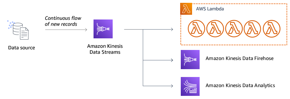
Before the release of Amazon Kinesis Data Analytics Studio, customers relied on Amazon Kinesis Data Analytics for SQL on Amazon Kinesis Data Streams. With the release of Kinesis Data Analytics Studio, data engineers and analysts can use an Apache Zeppelin notebook within Studio to query streaming data interactively from a variety of sources, like Kinesis Data Streams, Amazon Managed Streaming for Apache Kafka (Amazon MSK), Amazon Simple Storage Service (Amazon S3), and other sources using custom connectors.
In this post, we cover some of the most common query patterns to run on streaming data using Apache Flink relational APIs. Out of the two relational API types supported by Apache Flink, SQL and Table APIs, our focus is on SQL APIs. We expect readers to have knowledge of Kinesis Data Streams, AWS Glue, and AWS Identity and Access Management (IAM). In this post, we use a sales transaction use case to walk you through the examples of tumbling, sliding, session and windows, group by, and joins query operations. We expect readers to have a basic knowledge of SQL queries and streaming window concepts.
Solution architecture
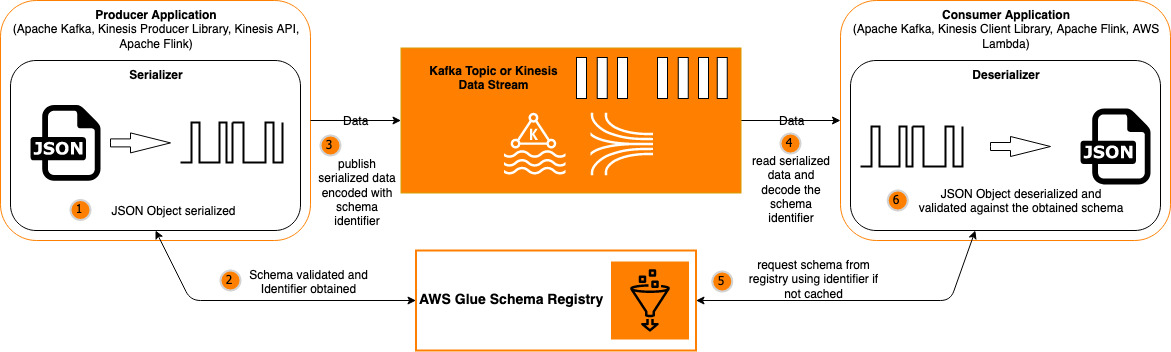
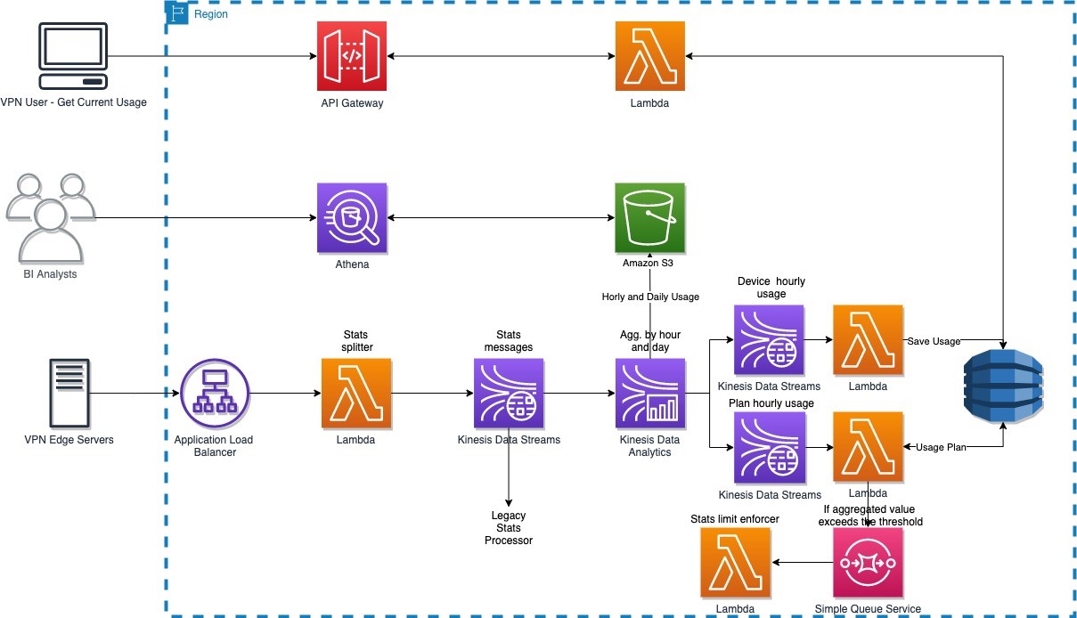
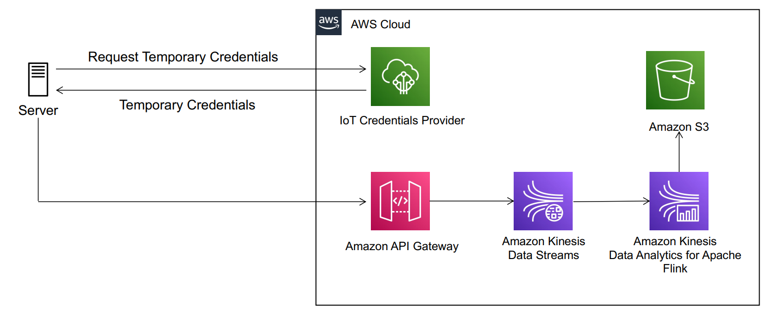
To show the working solution of interactive analytics on streaming data, we use a Kinesis Data Generator UI application to generate the stream of data, which continuously writes to Kinesis Data Streams. For the interactive analytics on Kinesis Data Streams, we use Kinesis Data Analytics Studio that uses Apache Flink as the processing engine, and notebooks powered by Apache Zeppelin. These notebooks come with preconfigured Apache Flink, which allows you to query data from Kinesis Data Streams interactively using SQL APIs. To use SQL queries in the Apache Zeppelin notebook, we configure an AWS Glue Data Catalog table, which is configured to use Kinesis Data Streams as a source. This configuration allows you to query the data stream by referring to the AWS Glue table in SQL queries.
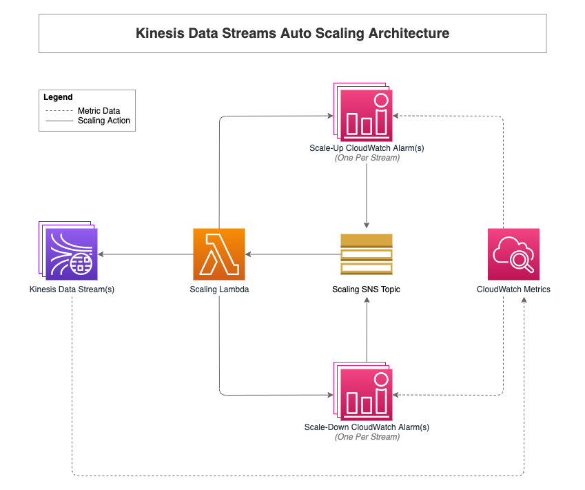
We use an AWS CloudFormation template to create the AWS resources shown in the following diagram.

Set up the environment
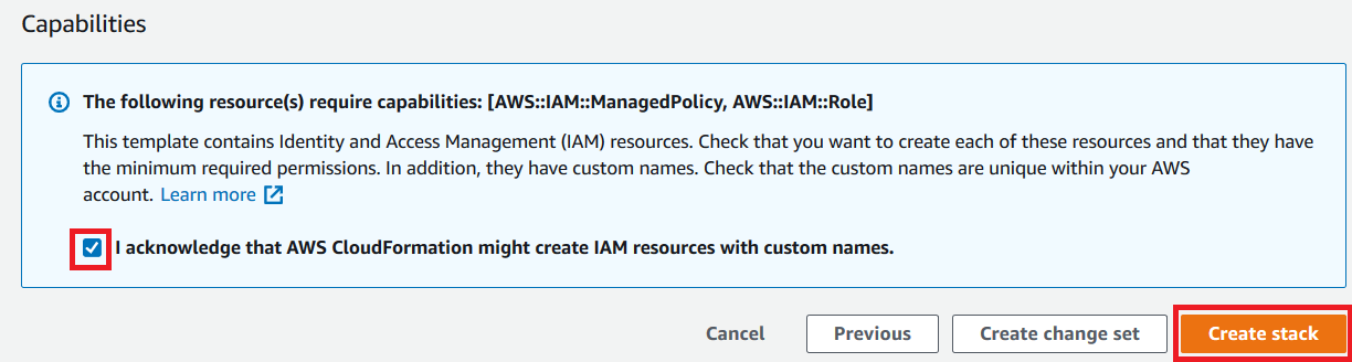
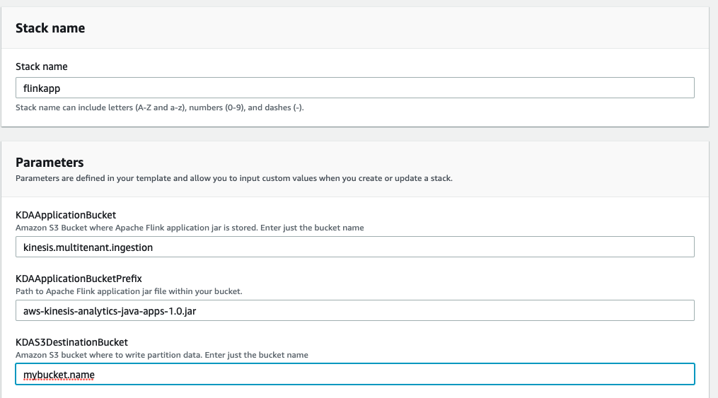
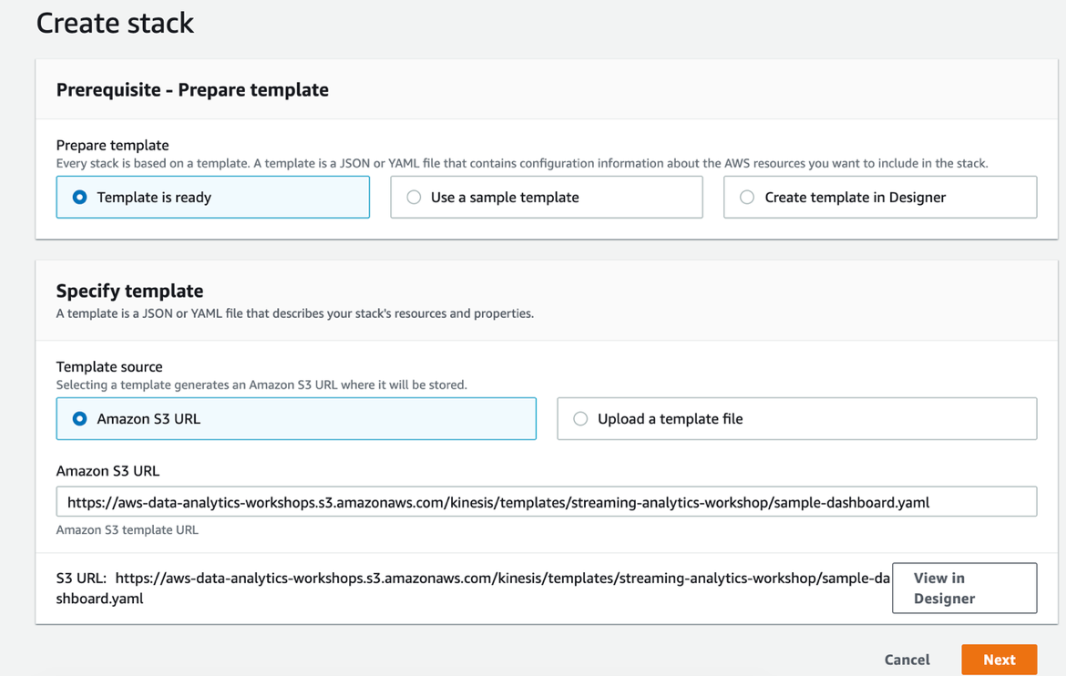
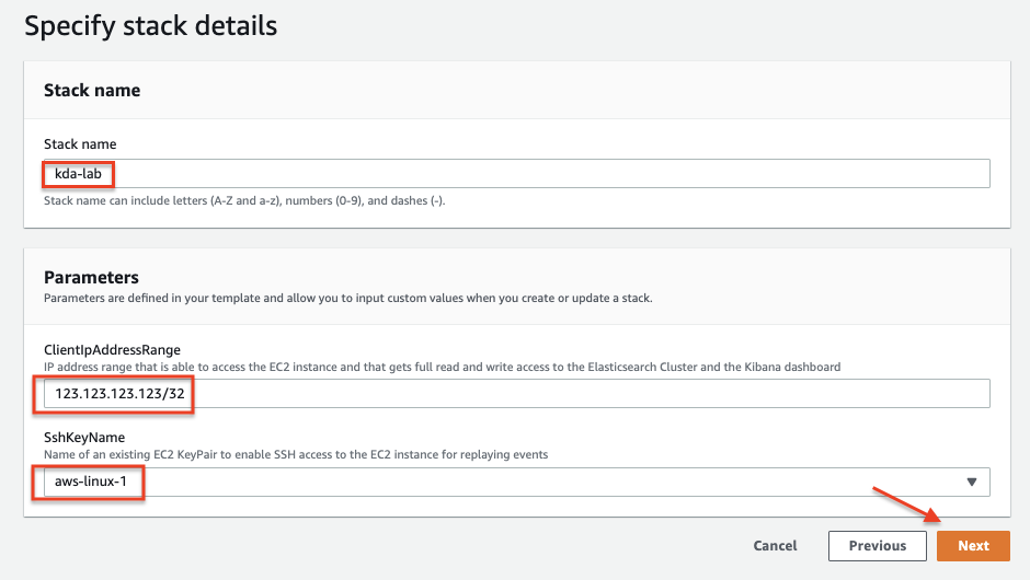
After you sign in to your AWS account, launch the CloudFormation template by choosing Launch Stack:

The CloudFormation template configures the following resources in your account:
- Two Kinesis data streams, one for sales transactions and one for card data
- A Kinesis Data Analytics Studio application
- An IAM role (service execution role) for Kinesis Data Analytics Studio
- Two AWS Glue Data Catalog tables:
sales and card
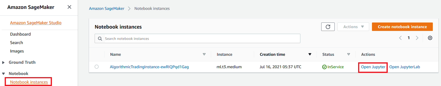
After you complete the setup, sign in to the Kinesis Data Analytics console. On the Kinesis Data Analytics applications page, choose the Studio tab, where you can see the Studio notebook in ready status. Select the Studio notebook, choose Run, and wait until the notebook is in running status. It can take a couple of minutes for the notebook to get into running status.

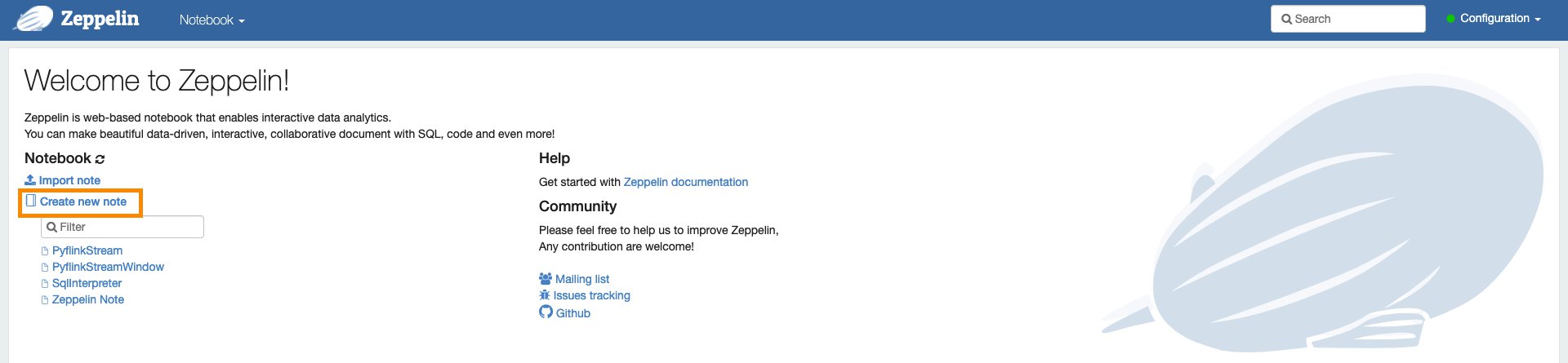
To run the analysis on streaming data, select the Apache Zeppelin notebook environment and open it. You have the option to create a new note in the notebook.

Run stream analytics in an interactive application
Before you start running interactive analytics with a Studio notebook, you need to start streaming data into your Kinesis data stream, which you created earlier using the CloudFormation stack. To generate streaming data into the data stream, we use a hosted Kinesis Data Generator UI application.
- Create an Amazon Cognito user pool in your account and user in that pool. For instructions, see the GitHub repo.
- Log in to the Kinesis Data Generator application.
- Choose the Region where the CloudFormation template was run to create the Kinesis data stream.
- Choose the data stream from the drop-down menu and select the data stream for
sales.
- Set records per second to 10.
- Use the following code for the record template:
{
    "customer_card_id": {{random.number({
            "min":1,
            "max":99
        })}},
    "customer_id": {{random.number({
            "min":100,
            "max":110
        })}},
    "price": {{random.number(
        {
            "min":10,
            "max":500
        }
    )}},
    "product_id": "{{random.arrayElement(
        ["4E5750DC2A1D","E6DA5387367B","B552B4B940D0"]
    )}}"
}
- Choose Send Data.
To run the table join queries in the example section, you need to stream sample card data to a separate data stream.
- Choose the Region where you created the data stream.
- Choose the data stream from the drop-down menu.
- Select the data stream for
card.
- Set records per second to 5.
- Use the following code for the record template:
{
    "card_id": {{random.number({
            "min":75,
            "max":99
        })}},
    "card_number": {{random.number({
            "min":23274397,
            "max":47547920
        })}},
    "card_zip": "{{random.arrayElement(
        ["07422","23738","03863"]
    )}}",
    "card_name": "{{random.arrayElement(
        ["Laura Perez","Peter Han","Karla Johnson"]
    )}}"
}
- Choose Send Data.
- Go back to the notebook note and specify the language Studio uses to run the application.
You need to specify Flink interpreter supported by Apache Zeppelin notebook, like Python, IPython, stream SQL, or batch SQL. Because we use Python Flink streaming SQL APIs in this post, we use the stream SQL interpreter ssql as the first statement:
Common query patterns with Flink SQL
In this section, we walk you through examples of common query patterns using Flink SQL APIs. In all the examples, we refer to the sales table, which is the AWS Glue table created by the CloudFormation template that has Kinesis Data Streams as a source. It’s the same data stream where you publish the sales data using the Kinesis Data Generator application.
Windows and aggregation
In this section, we cover examples of windowed and aggregate queries: tumbling, sliding, and session window operations.
Tumbling window
In the following example, we use SUM aggregation on a tumbling window. The query emits the total spend for every customer every 30-second window interval.
The following table shows our input data.
| proctime |
customer_id |
customer_card_id |
product_id |
price |
| 2021-04-20 21:31:01.10 |
75 |
101 |
4E5750DC2A1D |
110 |
| 2021-04-20 21:31:01.115 |
78 |
118 |
B552B4B940D0 |
80 |
| 2021-04-20 21:31:01.328 |
75 |
101 |
E6DA5387367B |
60 |
| 2021-04-20 21:31:01.504 |
78 |
101 |
4E5750DC2A1D |
110 |
| 2021-04-20 21:31:01.678 |
75 |
148 |
4E5750DC2A1D |
110 |
| 2021-04-20 21:31:01.960 |
78 |
118 |
B552B4B940D0 |
80 |
We use the following code for our query:
%flink.ssql(type=update)
SELECT TUMBLE_END(proctime, INTERVAL '30' SECOND) as window_end_time, customer_id
, SUM(price) as tumbling_30_seconds_sum
FROM sales
GROUP BY TUMBLE(proctime, INTERVAL '30' SECOND), customer_id
The following table shows our results.
| windown_end_time |
customer_id |
tumbling_30_seconds_sum |
| 2021-04-20 21:31:01.0 |
75 |
170 |
| 2021-04-20 21:31:01.0 |
78 |
80 |
| 2021-04-20 21:31:30.0 |
75 |
110 |
| 2021-04-20 21:31:30.0 |
78 |
190 |
Sliding window
In this sliding window example, we run a SUM aggregate query that emits the total spend for every customer every 10 seconds for the 30-second window.
The following table shows our input data.
| proctime |
customer_id |
customer_card_id |
product_id |
price |
| 2021-04-20 21:31:01.10 |
75 |
101 |
4E5750DC2A1D |
110 |
| 2021-04-20 21:31:01.20 |
78 |
118 |
B552B4B940D0 |
80 |
| 2021-04-20 21:31:01.28 |
75 |
101 |
E6DA5387367B |
60 |
| 2021-04-20 21:31:01.30 |
78 |
101 |
4E5750DC2A1D |
110 |
| 2021-04-20 21:31:01.36 |
75 |
148 |
4E5750DC2A1D |
110 |
| 2021-04-20 21:31:01.40 |
78 |
118 |
B552B4B940D0 |
80 |
We use the following code for our query:
%flink.ssql(type=update)
SELECT HOP_END(proctime, INTERVAL '10' SECOND, INTERVAL '30' SECOND) AS window_end_time
, customer_id, SUM(price) AS sliding_30_seconds_sum
FROM sales
GROUP BY HOP(proctime, INTERVAL '10' SECOND, INTERVAL '30' SECOND), customer_id
The following table shows our results.
| window_end_time |
customer_id |
sliding_30_seconds_sum |
| 2021-04-20 21:31:01.10 |
75 |
110 |
| 2021-04-20 21:31:01.20 |
75 |
110 |
| 2021-04-20 21:31:01.20 |
78 |
80 |
| 2021-04-20 21:31:30.30 |
75 |
170 |
| 2021-04-20 21:31:30.30 |
78 |
190 |
| 2021-04-20 21:31:30.40 |
75 |
280 |
| 2021-04-20 21:31:30.40 |
78 |
270 |
Session window
The following example of a session window query finds the total spend per session for a 1-minute gap of inactivity. To generate the result, we stream the data from the Kinesis Data Generator application and stop streaming for more than a minute to create a 1-minute gap of inactivity.
The following table shows our input data.
| proctime |
customer_id |
customer_card_id |
product_id |
price |
| 2021-04-20 21:31:01.10 |
75 |
101 |
4E5750DC2A1D |
110 |
| 2021-04-20 21:31:01.20 |
78 |
118 |
B552B4B940D0 |
80 |
| 2021-04-20 21:31:01.28 |
75 |
101 |
E6DA5387367B |
60 |
| 2021-04-20 21:32:50.30 |
78 |
101 |
4E5750DC2A1D |
110 |
| 2021-04-20 21:32:50.36 |
75 |
148 |
4E5750DC2A1D |
110 |
We use the following code for our query:
%flink.ssql(type=update)
SELECT customer_id, SESSION_START(proctime, INTERVAL '1' MINUTE) AS session_start_time
, SESSION_PROCTIME(proctime, INTERVAL '1' MINUTE) AS session_end_time, SUM(price) AS total_spend
FROM sales
GROUP BY SESSION(proctime, INTERVAL '1' MINUTE), customer_id
The following table shows our results.
| session_start_time |
session_end_time |
total_spend |
| 2021-04-20 21:31:01.10 |
2021-04-20 21:32:01.28 |
250 |
| 2021-04-20 21:32:50.30 |
2021-04-20 21:32:50.36 |
220 |
Data filter and consolidation
To show an example of a filter and union operation, we create two separate datasets using the filter condition and combine them using the UNION operation.
The following table shows our input data.
| proctime |
customer_id |
customer_card_id |
product_id |
price |
| 2021-04-20 21:31:01.10 |
75 |
101 |
4E5750DC2A1D |
110 |
| 2021-04-20 21:31:01.20 |
78 |
118 |
B552B4B940D0 |
80 |
| 2021-04-20 21:31:01.28 |
75 |
101 |
E6DA5387367B |
60 |
| 2021-04-20 21:32:50.30 |
78 |
101 |
4E5750DC2A1D |
110 |
| 2021-04-20 21:32:50.36 |
75 |
148 |
4E5750DC2A1D |
110 |
We use the following code for our query:
%flink.ssql(type=update)
SELECT * FROM (
(SELECT customer_id, product_id, price FROM sales WHERE price > 100 AND  product_id <> '4E5750DC2A1D')
UNION
(SELECT customer_id, product_id, price FROM sales WHERE product_id = '4E5750DC2A1D' AND price > 250)
)
The following table shows our results.
| customer_id |
product_id |
price |
| 78 |
4E5750DC2A1D |
300 |
| 75 |
B552B4B940D0 |
170 |
| 78 |
B552B4B940D0 |
110 |
| 75 |
4E5750DC2A1D |
260 |
Table joins
Flink SQL APIs support different types of join conditions, like inner join, outer join, and interval join. You want to limit the resource utilization from growing indefinitely, and run joins effectively. For that reason, in our example, we use table joins using an interval join. An interval join requires one equi-join predicate and a join condition that bounds the time on both sides. In this example, we join the dataset of two Kinesis Data Streams tables based on the card ID, which is a common field between the two stream datasets. The filter condition in the query is based on a time constraint, which restricts resource utilization from growing.
The following table shows our sales input data.
| proctime |
customer_id |
customer_card_id |
product_id |
price |
| 2021-04-20 21:31:01.10 |
75 |
101 |
4E5750DC2A1D |
110 |
| 2021-04-20 21:31:01.20 |
78 |
118 |
B552B4B940D0 |
80 |
| 2021-04-20 21:31:01.28 |
75 |
101 |
E6DA5387367B |
60 |
| 2021-04-20 21:32:50.30 |
78 |
101 |
4E5750DC2A1D |
110 |
| 2021-04-20 21:32:50.36 |
75 |
148 |
4E5750DC2A1D |
110 |
The following table shows our cards input data.
| card_id |
card_number |
card_zip |
card_name |
| 101 |
23274397 |
23738 |
Laura Perez |
| 118 |
54093472 |
7422 |
Karla Johnson |
| 101 |
23274397 |
23738 |
Laura Perez |
| 101 |
23274397 |
23738 |
Laura Perez |
| 148 |
91368810 |
7422 |
Peter Han |
We use the following code for our query:
%flink.ssql(type=update)
SELECT sales.proctime, customer_card_id, card_zip, product_id, price
FROM card INNER JOIN sales ON card.card_id = sales.customer_card_id
WHERE sales.proctime BETWEEN card.proctime - INTERVAL '5' MINUTE AND card.proctime;
The following table shows our results.
| proctime |
customer_card_id |
card_zip |
product_id |
price |
| 2021-04-20 21:31:01.10 |
101 |
23738 |
4E5750DC2A1D |
110 |
| 2021-04-20 21:31:01.20 |
118 |
7422 |
B552B4B940D0 |
80 |
| 2021-04-20 21:31:01.28 |
101 |
23738 |
E6DA5387367B |
60 |
| 2021-04-20 21:32:50.30 |
101 |
23738 |
4E5750DC2A1D |
110 |
| 2021-04-20 21:32:50.36 |
148 |
7422 |
4E5750DC2A1D |
110 |
Data partitioning and ranking
To show the example of Top-N records, we use the same input dataset as in the previous join example. In this example, we run a query to find the top sales records by sales price in each zip code. We use the OVER window clause to rank sales in each zip code using a PARTITION BY clause. Next, we order the records in each zip code with an ORDER BY clause on the price field in descending order. The result of this operation is a ranking of each record based on the OVER clause condition. We use the external block of the query to filter the result on ranking so that we get the top sales in each zip code.
We use the following code for our query:
%flink.ssql(type=update)
SELECT card_zip, customer_card_id, product_id, price FROM (
SELECT *,
ROW_NUMBER() OVER (PARTITION BY card_zip ORDER BY price DESC) as row_num
FROM card INNER JOIN sales ON card.card_id = sales.customer_card_id
WHERE sales.proctime BETWEEN card.proctime - INTERVAL '5' MINUTE AND card.proctime
)
WHERE row_num = 1
The following table shows our results.
| card_zip |
customer_card_id |
product_id |
price |
| 23738 |
101 |
4E5750DC2A1D |
110 |
| 7422 |
148 |
4E5750DC2A1D |
110 |
Data transformation
There are times when you want to transform incoming data. The Flink SQL API has many built-in functions to support a wide range of data transformation requirements, including string functions, date functions, arithmetic functions, and so on. For the complete list, see System (Built-in) Functions.
Extract a portion of a string
In this example, we use the SUBSTR string function to subtract the first four digits and only return the last four digits of the card number.
The following table shows our sales input data.
| proctime |
customer_id |
customer_card_id |
product_id |
price |
| 2021-04-20 21:31:01.10 |
75 |
101 |
4E5750DC2A1D |
110 |
| 2021-04-20 21:31:01.20 |
78 |
118 |
B552B4B940D0 |
80 |
| 2021-04-20 21:31:01.28 |
75 |
101 |
E6DA5387367B |
60 |
| 2021-04-20 21:32:50.30 |
78 |
101 |
4E5750DC2A1D |
110 |
| 2021-04-20 21:32:50.36 |
75 |
148 |
4E5750DC2A1D |
110 |
The following table shows our cards input data.
| card_id |
card_number |
card_zip |
card_name |
| 101 |
23274397 |
23738 |
Laura Perez |
| 118 |
54093472 |
7422 |
Karla Johnson |
| 101 |
23274397 |
23738 |
Laura Perez |
| 101 |
23274397 |
23738 |
Laura Perez |
| 148 |
91368810 |
7422 |
Peter Han |
We use the following code for our query:
%flink.ssql(type=update)
SELECT proctime, SUBSTR(card_number,5) AS partial_card_number,    card_zip, product_id, price
FROM card INNER JOIN sales ON card.card_id = sales.customer_card_id
The following table shows our results.
| proctime |
partial_card_number |
card_zip |
product_id |
price |
| 2021-04-20 21:31:01.10 |
4397 |
23738 |
4E5750DC2A1D |
110 |
| 2021-04-20 21:31:01.20 |
3472 |
7422 |
B552B4B940D0 |
80 |
| 2021-04-20 21:31:01.28 |
4397 |
23738 |
E6DA5387367B |
60 |
| 2021-04-20 21:32:50.30 |
4397 |
23738 |
4E5750DC2A1D |
110 |
| 2021-04-20 21:32:50.36 |
8810 |
7422 |
4E5750DC2A1D |
110 |
Replace a substring
In this example, we use the REGEXP_REPLACE string function to remove all the characters after the space from the card_name field. Assuming that the first name and last name are separated by a space, the query returns the first name only.
The following table shows our cards input data.
| card_id |
card_number |
card_zip |
card_name |
| 101 |
23274397 |
23738 |
Laura Perez |
| 118 |
54093472 |
7422 |
Karla Johnson |
| 101 |
23274397 |
23738 |
Laura Perez |
| 101 |
23274397 |
23738 |
Laura Perez |
| 148 |
91368810 |
7422 |
Peter Han |
We use the following code for our query:
%flink.ssql(type=update)
SELECT card_id, REGEXP_REPLACE(card_name,' .*','') card_name
FROM card
The following table shows our results.
| card_id |
card_name |
| 101 |
Laura |
| 118 |
Karla |
| 101 |
Laura |
| 101 |
Laura |
| 148 |
Jason |
Split the string field into multiple fields
In this example, we use the SPLIT_INDEX string function to split the card_name field into first_name and last_name, assuming the card_name field is a full name separated by space.
The following table shows our cards input data.
| card_id |
card_number |
card_zip |
card_name |
| 101 |
23274397 |
23738 |
Laura Perez |
| 118 |
54093472 |
7422 |
Karla Johnson |
| 101 |
23274397 |
23738 |
Laura Perez |
| 101 |
23274397 |
23738 |
Laura Perez |
| 148 |
91368810 |
7422 |
Peter Han |
We use the following code for our query:
%flink.ssql(type=update)
SELECT card_id, SPLIT_INDEX(card_name,' ',0) first_name, SPLIT_INDEX(card_name,' ',1) last_name
FROM card
The following table shows our results.
| card_id |
first_name |
last_name |
| 101 |
Laura |
Perez |
| 118 |
Karla |
Johnson |
| 101 |
Laura |
Perez |
| 101 |
Laura |
Perez |
| 148 |
Peter |
Han |
Transform data using a CASE statement
There are times when you want to transform the result value and apply labels to get insights. For our example, we label the risk level as high, medium, or low for every customer (who is purchasing in the window) based on the number of purchases in the last 5-minute sliding window that emits results every 30 seconds.
The following table shows our input data.
| proctime |
customer_id |
customer_card_id |
product_id |
price |
| 2021-04-20 21:31:30.10 |
75 |
101 |
4E5750DC2A1D |
110 |
| 2021-04-20 21:31:38.20 |
78 |
118 |
B552B4B940D0 |
80 |
| 2021-04-20 21:31:42.28 |
75 |
101 |
E6DA5387367B |
60 |
| 2021-04-20 21:31:50.30 |
78 |
101 |
4E5750DC2A1D |
110 |
| 2021-04-20 21:31:50.36 |
75 |
148 |
4E5750DC2A1D |
110 |
We use the following code for our query:
%flink.ssql(type=update)
SELECT customer_id, CASE
WHEN total_purchases BETWEEN 1 AND 2 THEN 'LOW'
WHEN total_purchases BETWEEN 3 AND 10 THEN 'MEDIUM'
ELSE 'HIGH'
END as risk
FROM (
SELECT HOP_END(proctime, INTERVAL '30' SECOND, INTERVAL '5' MINUTE) AS winend
, customer_id, COUNT(1) AS total_purchases
FROM sales
GROUP BY HOP(proctime, INTERVAL '30' SECOND, INTERVAL '5' MINUTE), customer_id
)
The following table shows our results.
| customer_id |
risk |
| 78 |
LOW |
| 75 |
HIGH |
DateTime data transformation
The Flink SQL API has a wide range of built-in functions to operate on the date timestamp field, like extracting the day, month, week, hour, minute, day of the month, and so on. There are functions to convert the date timestamp field. In this example, we use the MINUTE and HOUR functions to extract the minute of an hour and the hour from the timestamp field.
The following table shows our sales input data.
| proctime |
customer_id |
customer_card_id |
product_id |
price |
| 2021-04-20 21:31:01.10 |
75 |
101 |
4E5750DC2A1D |
110 |
| 2021-04-20 21:31:01.20 |
78 |
118 |
B552B4B940D0 |
80 |
| 2021-04-20 21:31:01.28 |
75 |
101 |
E6DA5387367B |
60 |
| 2021-04-20 21:32:50.30 |
78 |
101 |
4E5750DC2A1D |
110 |
| 2021-04-20 21:32:50.36 |
75 |
148 |
4E5750DC2A1D |
110 |
We use the following code for our query:
%flink.ssql(type=update)
SELECT HOUR(TIMESTAMP proctime) AS transaction_hour, MINUTE(TIMESTAMP proctime) AS transaction_min,customer_id, product_id, price
FROM sales
The following table shows our results.
| transaction_hour |
transaction_min |
customer_id |
product_id |
price |
| 21 |
31 |
75 |
4E5750DC2A1D |
110 |
| 21 |
31 |
78 |
B552B4B940D0 |
80 |
| 21 |
31 |
75 |
E6DA5387367B |
60 |
| 21 |
32 |
78 |
4E5750DC2A1D |
110 |
| 21 |
32 |
75 |
4E5750DC2A1D |
110 |
Conclusion
In this post, we used sales and card examples to demonstrate different query patterns to get insight from streaming data using Apache Flink SQL APIs. We walked you through examples of Flink SQL queries that you can run within Kinesis Data Analytics Studio. In just a few minutes, you can start running interactive analytics with the examples in this post.
You can quickly start developing a stream processing application using Studio from the supported languages like SQL, Python, and Scala. If you want to generate continuous actionable insights, you can easily build and deploy your code as an Apache Flink application with durable state from the notebook within Studio. For more information, see Deploying as an application with durable state.
For further reading on Flink SQL queries that you can use in Kinesis Data Analytics Studio, visit the official page at Apache Flink 1.11 SQL Queries.
About the Authors
 Dr. Sam Mokhtari is a Senior Solutions Architect at AWS. His main area of depth is “Data & Analytics” and he published more than 30 influential articles in this field. He is also a respected data & analytics advisor who led several large-scale implementation projects across different industries including energy, health, telecom and transport.
 Mitesh Patel is a Senior Solutions Architect at AWS. He works with customers in SMB to help them develop scalable, secure and cost effective solutions in AWS. He enjoys helping customers in modernizing applications using microservices and implementing serverless analytics platform.