Post Syndicated from Ali Alemi original https://aws.amazon.com/blogs/big-data/exploring-real-time-streaming-for-generative-ai-applications/
Foundation models (FMs) are large machine learning (ML) models trained on a broad spectrum of unlabeled and generalized datasets. FMs, as the name suggests, provide the foundation to build more specialized downstream applications, and are unique in their adaptability. They can perform a wide range of different tasks, such as natural language processing, classifying images, forecasting trends, analyzing sentiment, and answering questions. This scale and general-purpose adaptability are what makes FMs different from traditional ML models. FMs are multimodal; they work with different data types such as text, video, audio, and images. Large language models (LLMs) are a type of FM and are pre-trained on vast amounts of text data and typically have application uses such as text generation, intelligent chatbots, or summarization.
Streaming data facilitates the constant flow of diverse and up-to-date information, enhancing the models’ ability to adapt and generate more accurate, contextually relevant outputs. This dynamic integration of streaming data enables generative AI applications to respond promptly to changing conditions, improving their adaptability and overall performance in various tasks.
To better understand this, imagine a chatbot that helps travelers book their travel. In this scenario, the chatbot needs real-time access to airline inventory, flight status, hotel inventory, latest price changes, and more. This data usually comes from third parties, and developers need to find a way to ingest this data and process the data changes as they happen.
Batch processing is not the best fit in this scenario. When data changes rapidly, processing it in a batch may result in stale data being used by the chatbot, providing inaccurate information to the customer, which impacts the overall customer experience. Stream processing, however, can enable the chatbot to access real-time data and adapt to changes in availability and price, providing the best guidance to the customer and enhancing the customer experience.
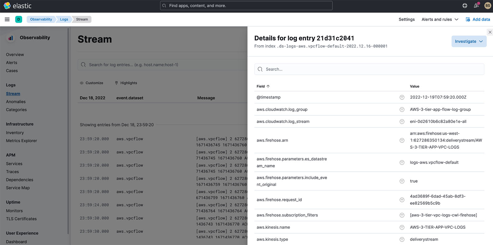
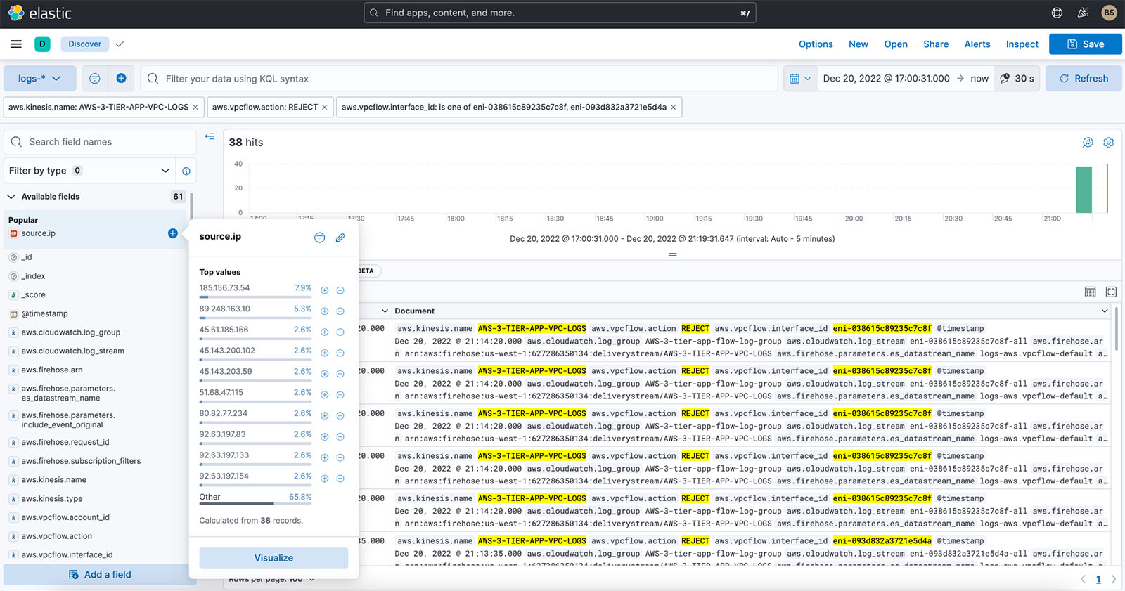
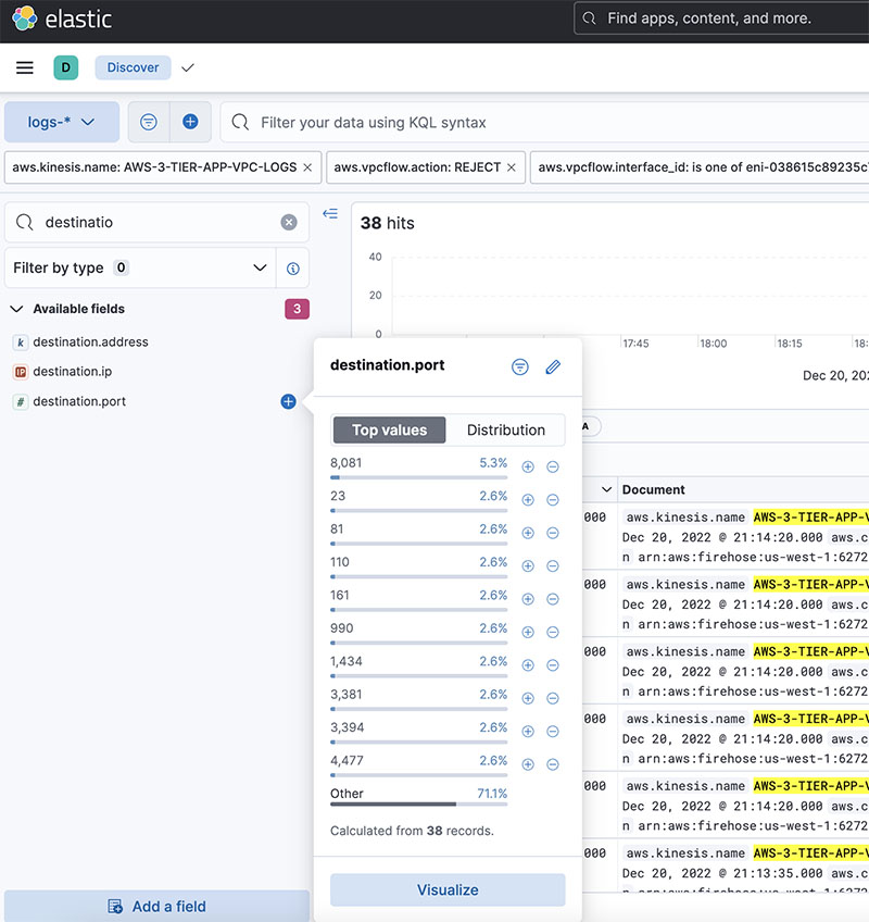
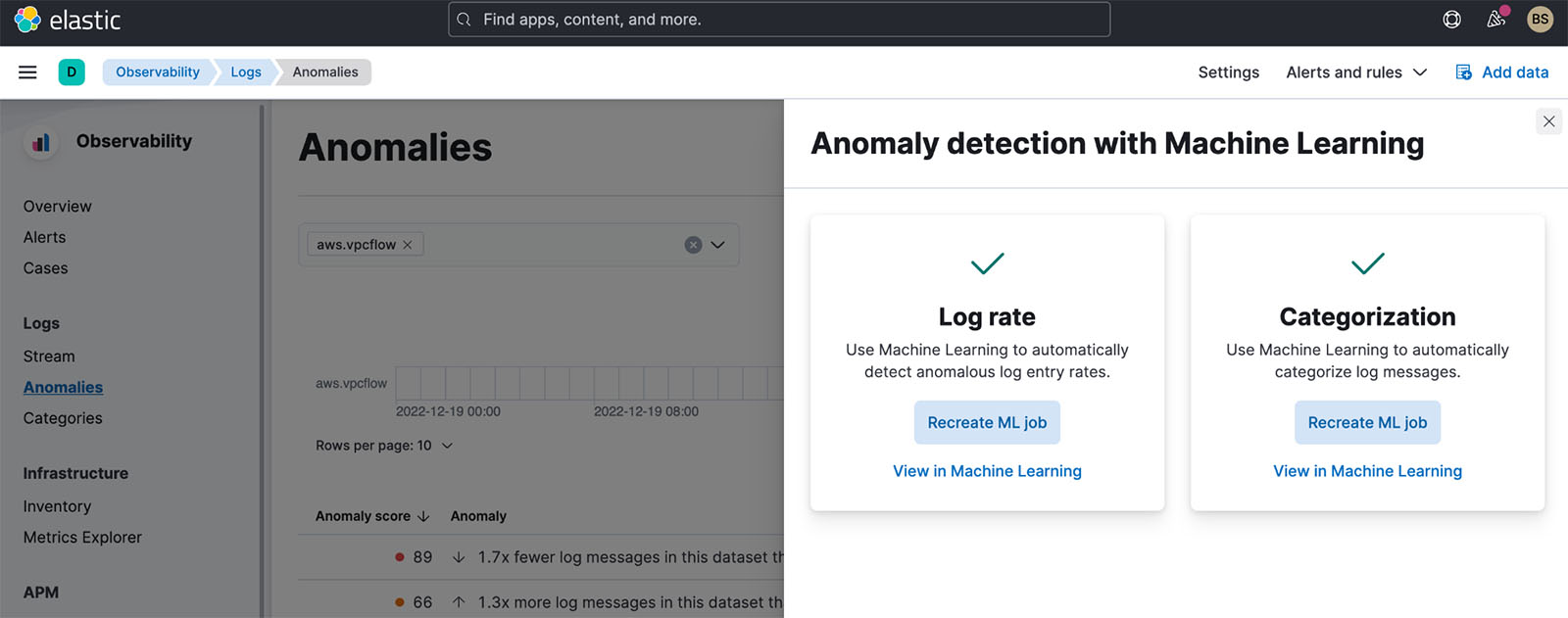
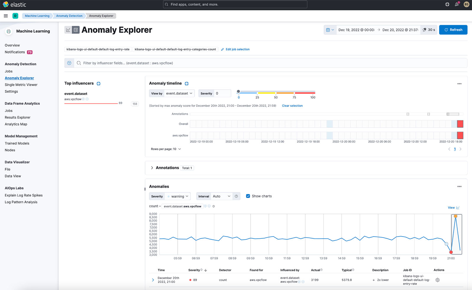
Another example is an AI-driven observability and monitoring solution where FMs monitor real-time internal metrics of a system and produces alerts. When the model finds an anomaly or abnormal metric value, it should immediately produce an alert and notify the operator. However, the value of such important data diminishes significantly over time. These notifications should ideally be received within seconds or even while it’s happening. If operators receive these notifications minutes or hours after they happened, such an insight is not actionable and has potentially lost its value. You can find similar use cases in other industries such as retail, car manufacturing, energy, and the financial industry.
In this post, we discuss why data streaming is a crucial component of generative AI applications due to its real-time nature. We discuss the value of AWS data streaming services such as Amazon Managed Streaming for Apache Kafka (Amazon MSK), Amazon Kinesis Data Streams, Amazon Managed Service for Apache Flink, and Amazon Kinesis Data Firehose in building generative AI applications.
In-context learning
LLMs are trained with point-in-time data and have no inherent ability to access fresh data at inference time. As new data appears, you will have to continuously fine-tune or further train the model. This is not only an expensive operation, but also very limiting in practice because the rate of new data generation far supersedes the speed of fine-tuning. Additionally, LLMs lack contextual understanding and rely solely on their training data, and are therefore prone to hallucinations. This means they can generate a fluent, coherent, and syntactically sound but factually incorrect response. They are also devoid of relevance, personalization, and context.
LLMs, however, have the capacity to learn from the data they receive from the context to more accurately respond without modifying the model weights. This is called in-context learning, and can be used to produce personalized answers or provide an accurate response in the context of organization policies.
For example, in a chatbot, data events could pertain to an inventory of flights and hotels or price changes that are constantly ingested to a streaming storage engine. Furthermore, data events are filtered, enriched, and transformed to a consumable format using a stream processor. The result is made available to the application by querying the latest snapshot. The snapshot constantly updates through stream processing; therefore, the up-to-date data is provided in the context of a user prompt to the model. This allows the model to adapt to the latest changes in price and availability. The following diagram illustrates a basic in-context learning workflow.

A commonly used in-context learning approach is to use a technique called Retrieval Augmented Generation (RAG). In RAG, you provide the relevant information such as most relevant policy and customer records along with the user question to the prompt. This way, the LLM generates an answer to the user question using additional information provided as context. To learn more about RAG, refer to Question answering using Retrieval Augmented Generation with foundation models in Amazon SageMaker JumpStart.
A RAG-based generative AI application can only produce generic responses based on its training data and the relevant documents in the knowledge base. This solution falls short when a near-real-time personalized response is expected from the application. For example, a travel chatbot is expected to consider the user’s current bookings, available hotel and flight inventory, and more. Moreover, the relevant customer personal data (commonly known as the unified customer profile) is usually subject to change. If a batch process is employed to update the generative AI’s user profile database, the customer may receive dissatisfying responses based on old data.
In this post, we discuss the application of stream processing to enhance a RAG solution used for building question answering agents with context from real-time access to unified customer profiles and organizational knowledge base.
Near-real-time customer profile updates
Customer records are typically distributed across data stores within an organization. For your generative AI application to provide a relevant, accurate, and up-to-date customer profile, it is vital to build streaming data pipelines that can perform identity resolution and profile aggregation across the distributed data stores. Streaming jobs constantly ingest new data to synchronize across systems and can perform enrichment, transformations, joins, and aggregations across windows of time more efficiently. Change data capture (CDC) events contain information about the source record, updates, and metadata such as time, source, classification (insert, update, or delete), and the initiator of the change.
The following diagram illustrates an example workflow for CDC streaming ingestion and processing for unified customer profiles.

In this section, we discuss the main components of a CDC streaming pattern required to support RAG-based generative AI applications.
CDC streaming ingestion
A CDC replicator is a process that collects data changes from a source system (usually by reading transaction logs or binlogs) and writes CDC events with the exact same order they occurred in a streaming data stream or topic. This involves a log-based capture with tools such as AWS Database Migration Service (AWS DMS) or open source connectors such as Debezium for Apache Kafka connect. Apache Kafka Connect is part of the Apache Kafka environment, allowing data to be ingested from various sources and delivered to variety of destinations. You can run your Apache Kafka connector on Amazon MSK Connect within minutes without worrying about configuration, setup, and operating an Apache Kafka cluster. You only need to upload your connector’s compiled code to Amazon Simple Storage Service (Amazon S3) and set up your connector with your workload’s specific configuration.
There are also other methods for capturing data changes. For example, Amazon DynamoDB provides a feature for streaming CDC data to Amazon DynamoDB Streams or Kinesis Data Streams. Amazon S3 provides a trigger to invoke an AWS Lambda function when a new document is stored.
Streaming storage
Streaming storage functions as an intermediate buffer to store CDC events before they get processed. Streaming storage provides reliable storage for streaming data. By design, it is highly available and resilient to hardware or node failures and maintains the order of the events as they are written. Streaming storage can store data events either permanently or for a set period of time. This allows stream processors to read from part of the stream if there is a failure or a need for re-processing. Kinesis Data Streams is a serverless streaming data service that makes it straightforward to capture, process, and store data streams at scale. Amazon MSK is a fully managed, highly available, and secure service provided by AWS for running Apache Kafka.
Stream processing
Stream processing systems should be designed for parallelism to handle high data throughput. They should partition the input stream between multiple tasks running on multiple compute nodes. Tasks should be able to send the result of one operation to the next one over the network, making it possible for processing data in parallel while performing operations such as joins, filtering, enrichment, and aggregations. Stream processing applications should be able to process events with regards to the event time for use cases where events could arrive late or correct computation relies on the time events occur rather than the system time. For more information, refer to Notions of Time: Event Time and Processing Time.
Stream processes continuously produce results in the form of data events that need to be output to a target system. A target system could be any system that can integrate directly with the process or via streaming storage as in intermediary. Depending on the framework you choose for stream processing, you will have different options for target systems depending on available sink connectors. If you decide to write the results to an intermediary streaming storage, you can build a separate process that reads events and applies changes to the target system, such as running an Apache Kafka sink connector. Regardless of which option you choose, CDC data needs extra handling due to its nature. Because CDC events carry information about updates or deletes, it’s important that they merge in the target system in the right order. If changes are applied in the wrong order, the target system will be out of sync with its source.
Apache Flink is a powerful stream processing framework known for its low latency and high throughput capabilities. It supports event time processing, exactly-once processing semantics, and high fault tolerance. Additionally, it provides native support for CDC data via a special structure called dynamic tables. Dynamic tables mimic the source database tables and provide a columnar representation of the streaming data. The data in dynamic tables changes with every event that is processed. New records can be appended, updated, or deleted at any time. Dynamic tables abstract away the extra logic you need to implement for each record operation (insert, update, delete) separately. For more information, refer to Dynamic Tables.
With Amazon Managed Service for Apache Flink, you can run Apache Flink jobs and integrate with other AWS services. There are no servers and clusters to manage, and there is no compute and storage infrastructure to set up.
AWS Glue is a fully managed extract, transform, and load (ETL) service, which means AWS handles the infrastructure provisioning, scaling, and maintenance for you. Although it’s primarily known for its ETL capabilities, AWS Glue can also be used for Spark streaming applications. AWS Glue can interact with streaming data services such as Kinesis Data Streams and Amazon MSK for processing and transforming CDC data. AWS Glue can also seamlessly integrate with other AWS services such as Lambda, AWS Step Functions, and DynamoDB, providing you with a comprehensive ecosystem for building and managing data processing pipelines.
Unified customer profile
Overcoming the unification of the customer profile across a variety of source systems requires the development of robust data pipelines. You need data pipelines that can bring and synchronize all records into one data store. This data store provides your organization with the holistic customer records view that is needed for operational efficiency of RAG-based generative AI applications. For building such a data store, an unstructured data store would be best.
An identity graph is a useful structure for creating a unified customer profile because it consolidates and integrates customer data from various sources, ensures data accuracy and deduplication, offers real-time updates, connects cross-systems insights, enables personalization, enhances customer experience, and supports regulatory compliance. This unified customer profile empowers the generative AI application to understand and engage with customers effectively, and adhere to data privacy regulations, ultimately enhancing customer experiences and driving business growth. You can build your identity graph solution using Amazon Neptune, a fast, reliable, fully managed graph database service.
AWS provides a few other managed and serverless NoSQL storage service offerings for unstructured key-value objects. Amazon DocumentDB (with MongoDB compatibility) is a fast, scalable, highly available, and fully managed enterprise document database service that supports native JSON workloads. DynamoDB is a fully managed NoSQL database service that provides fast and predictable performance with seamless scalability.
Near-real-time organizational knowledge base updates
Similar to customer records, internal knowledge repositories such as company policies and organizational documents are siloed across storage systems. This is typically unstructured data and is updated in a non-incremental fashion. The use of unstructured data for AI applications is effective using vector embeddings, which is a technique of representing high dimensional data such as text files, images, and audio files as multi-dimensional numeric.
AWS provides several vector engine services, such as Amazon OpenSearch Serverless, Amazon Kendra, and Amazon Aurora PostgreSQL-Compatible Edition with the pgvector extension for storing vector embeddings. Generative AI applications can enhance the user experience by transforming the user prompt into a vector and use it to query the vector engine to retrieve contextually relevant information. Both the prompt and the vector data retrieved are then passed to the LLM to receive a more precise and personalized response.
The following diagram illustrates an example stream-processing workflow for vector embeddings.

Knowledge base contents need to be converted to vector embeddings before being written to the vector data store. Amazon Bedrock or Amazon SageMaker can help you access the model of your choice and expose a private endpoint for this conversion. Furthermore, you can use libraries such as LangChain to integrate with these endpoints. Building a batch process can help you convert your knowledge base content to vector data and store it in a vector database initially. However, you need to rely on an interval to reprocess the documents to synchronize your vector database with changes in your knowledge base content. With a large number of documents, this process can be inefficient. Between these intervals, your generative AI application users will receive answers according to the old content, or will receive an inaccurate answer because the new content is not vectorized yet.
Stream processing is an ideal solution for these challenges. It produces events as per existing documents initially and further monitors the source system and creates a document change event as soon as they occur. These events can be stored in streaming storage and wait to be processed by a streaming job. A streaming job reads these events, loads the content of the document, and transforms the contents to an array of related tokens of words. Each token further transforms into vector data via an API call to an embedding FM. Results are sent for storage to the vector storage via a sink operator.
If you’re using Amazon S3 for storing your documents, you can build an event-source architecture based on S3 object change triggers for Lambda. A Lambda function can create an event in the desired format and write that to your streaming storage.
You can also use Apache Flink to run as a streaming job. Apache Flink provides the native FileSystem source connector, which can discover existing files and read their contents initially. After that, it can continuously monitor your file system for new files and capture their content. The connector supports reading a set of files from distributed file systems such as Amazon S3 or HDFS with a format of plain text, Avro, CSV, Parquet, and more, and produces a streaming record. As a fully managed service, Managed Service for Apache Flink removes the operational overhead of deploying and maintaining Flink jobs, allowing you to focus on building and scaling your streaming applications. With seamless integration into the AWS streaming services such as Amazon MSK or Kinesis Data Streams, it provides features like automatic scaling, security, and resiliency, providing reliable and efficient Flink applications for handling real-time streaming data.
Based on your DevOps preference, you can choose between Kinesis Data Streams or Amazon MSK for storing the streaming records. Kinesis Data Streams simplifies the complexities of building and managing custom streaming data applications, allowing you to focus on deriving insights from your data rather than infrastructure maintenance. Customers using Apache Kafka often opt for Amazon MSK due to its straightforwardness, scalability, and dependability in overseeing Apache Kafka clusters within the AWS environment. As a fully managed service, Amazon MSK takes on the operational complexities associated with deploying and maintaining Apache Kafka clusters, enabling you to concentrate on constructing and expanding your streaming applications.
Because a RESTful API integration suits the nature of this process, you need a framework that supports a stateful enrichment pattern via RESTful API calls to track for failures and retry for the failed request. Apache Flink again is a framework that can do stateful operations in at-memory speed. To understand the best ways to make API calls via Apache Flink, refer to Common streaming data enrichment patterns in Amazon Kinesis Data Analytics for Apache Flink.
Apache Flink provides native sink connectors for writing data to vector datastores such as Amazon Aurora for PostgreSQL with pgvector or Amazon OpenSearch Service with VectorDB. Alternatively, you can stage the Flink job’s output (vectorized data) in an MSK topic or a Kinesis data stream. OpenSearch Service provides support for native ingestion from Kinesis data streams or MSK topics. For more information, refer to Introducing Amazon MSK as a source for Amazon OpenSearch Ingestion and Loading streaming data from Amazon Kinesis Data Streams.
Feedback analytics and fine-tuning
It’s important for data operation managers and AI/ML developers to get insight about the performance of the generative AI application and the FMs in use. To achieve that, you need to build data pipelines that calculate important key performance indicator (KPI) data based on the user feedback and variety of application logs and metrics. This information is useful for stakeholders to gain real-time insight about the performance of the FM, the application, and overall user satisfaction about the quality of support they receive from your application. You also need to collect and store the conversation history for further fine-tuning your FMs to improve their ability in performing domain-specific tasks.
This use case fits very well in the streaming analytics domain. Your application should store each conversation in streaming storage. Your application can prompt users about their rating of each answer’s accuracy and their overall satisfaction. This data can be in a format of a binary choice or a free form text. This data can be stored in a Kinesis data stream or MSK topic, and get processed to generate KPIs in real time. You can put FMs to work for users’ sentiment analysis. FMs can analyze each answer and assign a category of user satisfaction.
Apache Flink’s architecture allows for complex data aggregation over windows of time. It also provides support for SQL querying over stream of data events. Therefore, by using Apache Flink, you can quickly analyze raw user inputs and generate KPIs in real time by writing familiar SQL queries. For more information, refer to Table API & SQL.
With Amazon Managed Service for Apache Flink Studio, you can build and run Apache Flink stream processing applications using standard SQL, Python, and Scala in an interactive notebook. Studio notebooks are powered by Apache Zeppelin and use Apache Flink as the stream processing engine. Studio notebooks seamlessly combine these technologies to make advanced analytics on data streams accessible to developers of all skill sets. With support for user-defined functions (UDFs), Apache Flink allows for building custom operators to integrate with external resources such as FMs for performing complex tasks such as sentiment analysis. You can use UDFs to compute various metrics or enrich user feedback raw data with additional insights such as user sentiment. To learn more about this pattern, refer to Proactively addressing customer concern in real-time with GenAI, Flink, Apache Kafka, and Kinesis.
With Managed Service for Apache Flink Studio, you can deploy your Studio notebook as a streaming job with one click. You can use native sink connectors provided by Apache Flink to send the output to your storage of choice or stage it in a Kinesis data stream or MSK topic. Amazon Redshift and OpenSearch Service are both ideal for storing analytical data. Both engines provide native ingestion support from Kinesis Data Streams and Amazon MSK via a separate streaming pipeline to a data lake or data warehouse for analysis.
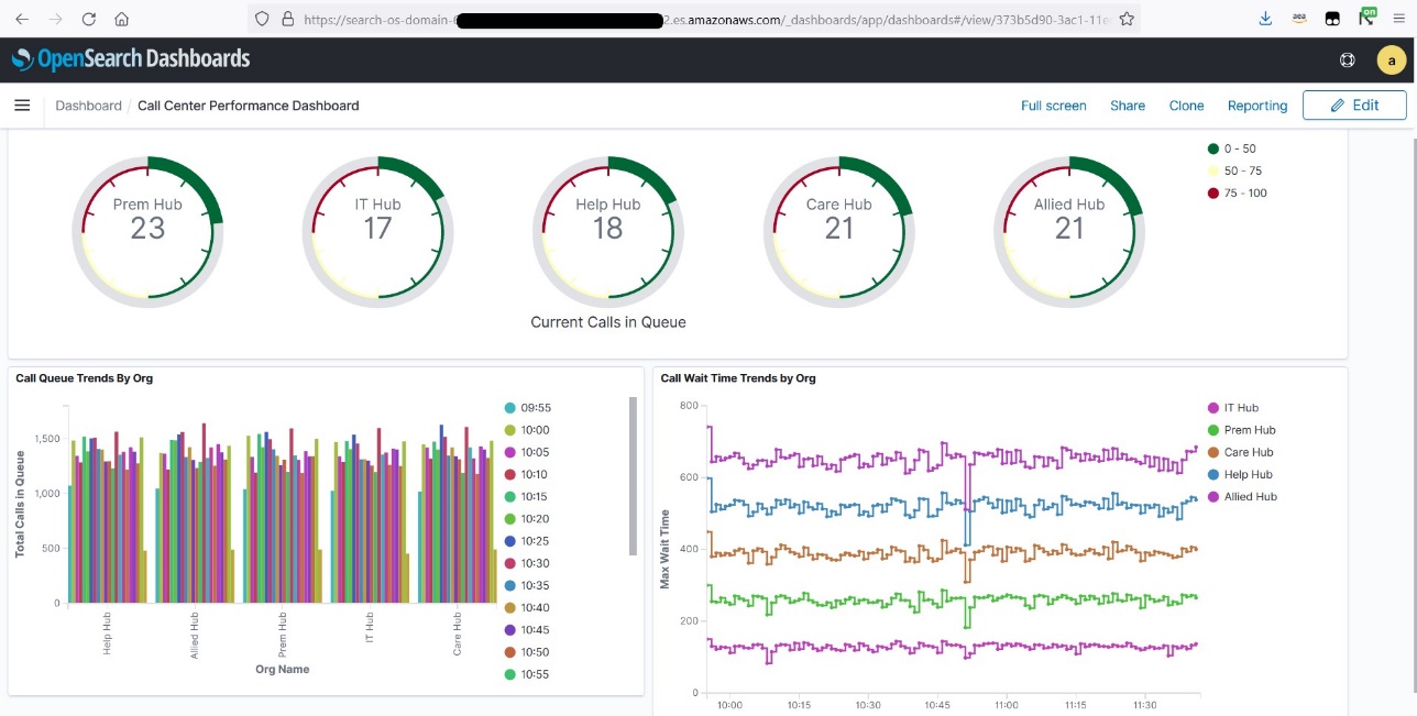
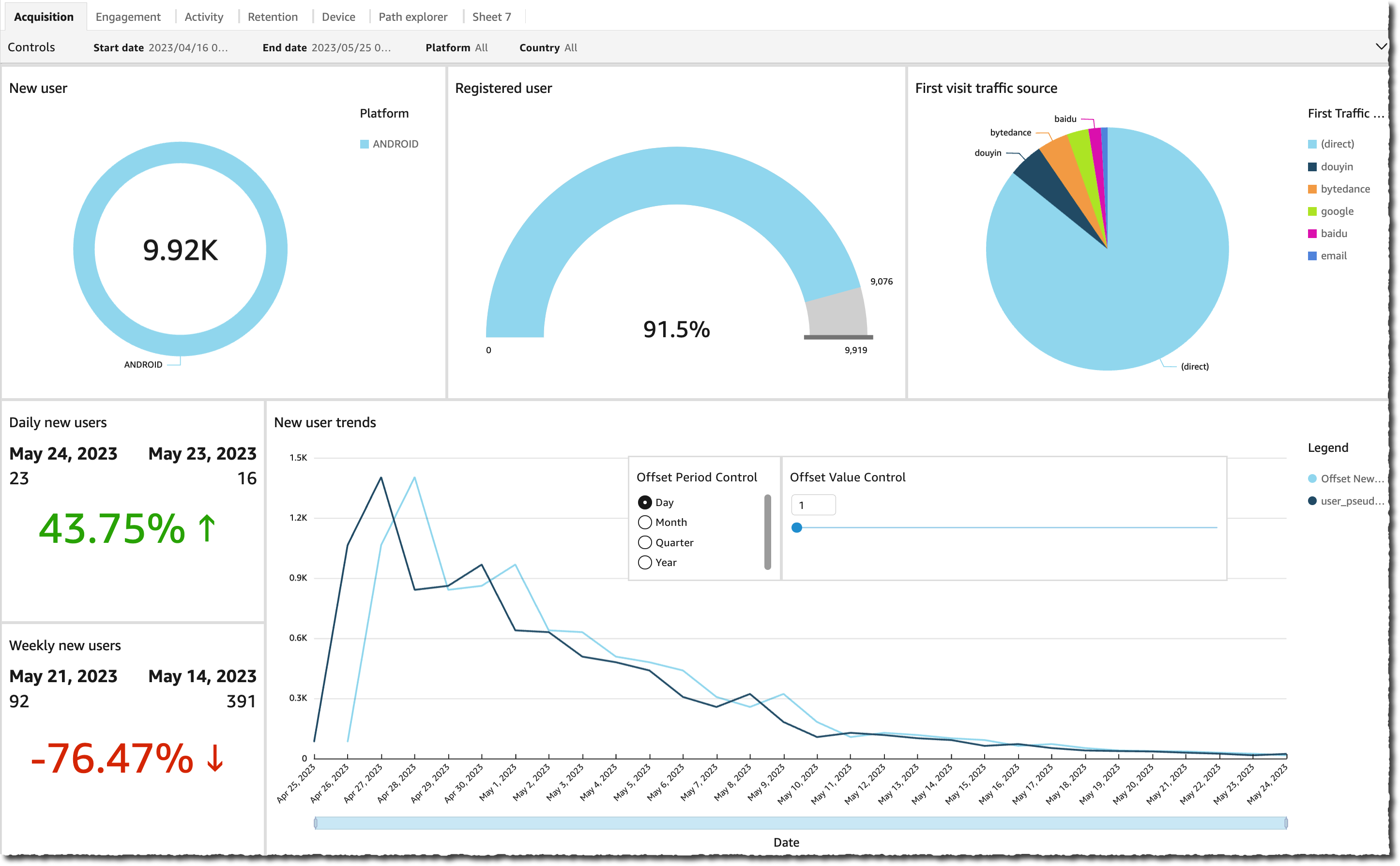
Amazon Redshift uses SQL to analyze structured and semi-structured data across data warehouses and data lakes, using AWS-designed hardware and machine learning to deliver the best price-performance at scale. OpenSearch Service offers visualization capabilities powered by OpenSearch Dashboards and Kibana (1.5 to 7.10 versions).
You can use the outcome of such analysis combined with user prompt data for fine-tuning the FM when is needed. SageMaker is the most straightforward way to fine-tune your FMs. Using Amazon S3 with SageMaker provides a powerful and seamless integration for fine-tuning your models. Amazon S3 serves as a scalable and durable object storage solution, enabling straightforward storage and retrieval of large datasets, training data, and model artifacts. SageMaker is a fully managed ML service that simplifies the entire ML lifecycle. By using Amazon S3 as the storage backend for SageMaker, you can benefit from the scalability, reliability, and cost-effectiveness of Amazon S3, while seamlessly integrating it with SageMaker training and deployment capabilities. This combination enables efficient data management, facilitates collaborative model development, and makes sure that ML workflows are streamlined and scalable, ultimately enhancing the overall agility and performance of the ML process. For more information, refer to Fine-tune Falcon 7B and other LLMs on Amazon SageMaker with @remote decorator.
With a file system sink connector, Apache Flink jobs can deliver data to Amazon S3 in open format (such as JSON, Avro, Parquet, and more) files as data objects. If you prefer to manage your data lake using a transactional data lake framework (such as Apache Hudi, Apache Iceberg, or Delta Lake), all of these frameworks provide a custom connector for Apache Flink. For more details, refer to Create a low-latency source-to-data lake pipeline using Amazon MSK Connect, Apache Flink, and Apache Hudi.
Summary
For a generative AI application based on a RAG model, you need to consider building two data storage systems, and you need to build data operations that keep them up to date with all the source systems. Traditional batch jobs are not sufficient to process the size and diversity of the data you need to integrate with your generative AI application. Delays in processing the changes in source systems result in an inaccurate response and reduce the efficiency of your generative AI application. Data streaming enables you to ingest data from a variety of databases across various systems. It also allows you to transform, enrich, join, and aggregate data across many sources efficiently in near-real time. Data streaming provides a simplified data architecture to collect and transform users’ real-time reactions or comments on the application responses, helping you deliver and store the results in a data lake for model fine-tuning. Data streaming also helps you optimize data pipelines by processing only the change events, allowing you to respond to data changes more quickly and efficiently.
Learn more about AWS data streaming services and get started building your own data streaming solution.
About the Authors
 Ali Alemi is a Streaming Specialist Solutions Architect at AWS. Ali advises AWS customers with architectural best practices and helps them design real-time analytics data systems which are reliable, secure, efficient, and cost-effective. He works backward from customer’s use cases and designs data solutions to solve their business problems. Prior to joining AWS, Ali supported several public sector customers and AWS consulting partners in their application modernization journey and migration to the Cloud.
 Imtiaz (Taz) Sayed is the World-Wide Tech Leader for Analytics at AWS. He enjoys engaging with the community on all things data and analytics. He can be reached via LinkedIn.


 Ranjit Kalidasan is a Senior Solutions Architect with Amazon Web Services based in Boston, Massachusetts. He is a Partner Solutions Architect helping security ISV partners co-build and co-market solutions with AWS. He brings over 25 years of experience in information technology helping global customers implement complex solutions for security and analytics. You can connect with Ranjit on LinkedIn.
 Phaneendra Vuliyaragoli is a Product Management Lead for Amazon Data Firehose at AWS. In this role, Phaneendra leads the product and go-to-market strategy for Amazon Data Firehose.

 Florian Mair is a Senior Solutions Architect and data streaming expert at AWS. He is a technologist that helps customers in Europe succeed and innovate by solving business challenges using AWS Cloud services. Besides working as a Solutions Architect, Florian is a passionate mountaineer, and has climbed some of the highest mountains across Europe.
 Emil Dietl is a Senior Tech Lead at Krones specializing in data engineering, with a key field in Apache Flink and microservices. His work often involves the development and maintenance of mission-critical software. Outside of his professional life, he deeply values spending quality time with his family.
 Simon Peyer is a Solutions Architect at AWS based in Switzerland. He is a practical doer and is passionate about connecting technology and people using AWS Cloud services. A special focus for him is data streaming and automations. Besides work, Simon enjoys his family, the outdoors, and hiking in the mountains.


 Ali Alemi is a Streaming Specialist Solutions Architect at AWS. Ali advises AWS customers with architectural best practices and helps them design real-time analytics data systems which are reliable, secure, efficient, and cost-effective. He works backward from customer’s use cases and designs data solutions to solve their business problems. Prior to joining AWS, Ali supported several public sector customers and AWS consulting partners in their application modernization journey and migration to the Cloud.
 Imtiaz (Taz) Sayed is the World-Wide Tech Leader for Analytics at AWS. He enjoys engaging with the community on all things data and analytics. He can be reached via
 Pratik Patel is Sr. Technical Account Manager and streaming analytics specialist. He works with AWS customers and provides ongoing support and technical guidance to help plan and build solutions using best practices and proactively keep customers’ AWS environments operationally healthy.
 Amar is a Senior Solutions Architect at Amazon AWS in the UK. He works across power, utilities, manufacturing and automotive customers on strategic implementations, specializing in using AWS Streaming and advanced data analytics solutions, to drive optimal business outcomes.


 Roy (KDS) Wang is a Senior Product Manager with Amazon Kinesis Data Streams. He is passionate about learning from and collaborating with customers to help organizations run faster and smarter. Outside of work, Roy strives to be a good dad to his new son and builds plastic model kits.
 Masudur Rahaman Sayem is a Streaming Data Architect at AWS. He works with AWS customers globally to design and build data streaming architectures to solve real-world business problems. He specializes in optimizing solutions that use streaming data services and NoSQL. Sayem is very passionate about distributed computing.


 Raj Ramasubbu is a Sr. Analytics Specialist Solutions Architect focused on big data and analytics and AI/ML with Amazon Web Services. He helps customers architect and build highly scalable, performant, and secure cloud-based solutions on AWS. Raj provided technical expertise and leadership in building data engineering, big data analytics, business intelligence, and data science solutions for over 18 years prior to joining AWS. He helped customers in various industry verticals like healthcare, medical devices, life science, retail, asset management, car insurance, residential REIT, agriculture, title insurance, supply chain, document management, and real estate.
 Rahul Sonawane is a Principal Analytics Solutions Architect at AWS with AI/ML and Analytics as his area of specialty.
 Sundeep Kumar is a Sr. Data Architect, Data Lake at AWS, helping customers build data lake and analytics platform and solutions. When not building and designing data lakes, Sundeep enjoys listening music and playing guitar.
 Deepthi Mohan is a Principal Product Manager on the Amazon Kinesis Data Analytics team.
 Karthi Thyagarajan was a Principal Solutions Architect on the Amazon Kinesis team.


 Chaitanya Shah is a Sr. Technical Account Manager(TAM) with AWS, based out of New York. He has over 22 years of experience working with enterprise customers. He loves to code and actively contributes to the AWS solutions labs to help customers solve complex problems. He provides guidance to AWS customers on best practices for their AWS Cloud migrations. He is also specialized in AWS data transfer and the data and analytics domain.


 Jeremy Ber has been working in the telemetry data space for the past 9 years as a Software Engineer, Machine Learning Engineer, and most recently a Data Engineer. At AWS, he is a Streaming Specialist Solutions Architect, supporting both Amazon Managed Streaming for Apache Kafka (Amazon MSK) and AWS’s managed offering for Apache Flink.
 Gaurav Rele is a Data Scientist at the Amazon ML Solution Lab, where he works with AWS customers across different verticals to accelerate their use of machine learning and AWS Cloud services to solve their business challenges.
 Antonio Vespoli is a Software Development Engineer in AWS. He works on Amazon Kinesis Data Analytics, the managed offering for running Apache Flink applications on AWS.
 Samuel Siebenmann is a Software Development Engineer in AWS. He works on Amazon Kinesis Data Analytics, the managed offering for running Apache Flink applications on AWS.
 Nuno Afonso is a Software Development Engineer in AWS. He works on Amazon Kinesis Data Analytics, the managed offering for running Apache Flink applications on AWS.


 Daren Wong is a Software Development Engineer in AWS. He works on Amazon Kinesis Data Analytics, the managed offering for running Apache Flink applications on AWS.
 Aleksandr Pilipenko is a Software Development Engineer in AWS. He works on Amazon Kinesis Data Analytics, the managed offering for running Apache Flink applications on AWS.
 Hong Liang Teoh is a Software Development Engineer in AWS. He works on Amazon Kinesis Data Analytics, the managed offering for running Apache Flink applications on AWS.


 Udayasimha Theepireddy is an Elastic Principal Solution Architect, where he works with customers to solve real world technology problems using Elastic and AWS services. He has a strong background in technology, business, and analytics.
 Antony Prasad Thevaraj is a Sr. Partner Solutions Architect in Data and Analytics at AWS. He has over 12 years of experience as a Big Data Engineer, and has worked on building complex ETL and ELT pipelines for various business units.
 Mostafa Mansour is a Principal Product Manager – Tech at Amazon Web Services where he works on Amazon Kinesis Data Firehose. He specializes in developing intuitive product experiences that solve complex challenges for customers at scale. When he’s not hard at work on Amazon Kinesis Data Firehose, you’ll likely find Mostafa on the squash court, where he loves to take on challengers and perfect his dropshots.


 Dhiraj Thakur is a Solutions Architect with Amazon Web Services. He works with AWS customers and partners to provide guidance on enterprise cloud adoption, migration, and strategy. He is passionate about technology and enjoys building and experimenting in the analytics and AI/ML space.
 Rajdip Chaudhuri is Solutions Architect with Amazon Web Services specializing in data and analytics. He enjoys working with AWS customers and partners on data and analytics requirements. In his spare time, he enjoys soccer.


 Raghu Boppanna works as an Enterprise Architect at Vanguard’s Chief Technology Office. Raghu specializes in Data Analytics, Data Migration/Replication including CDC Pipelines, Disaster Recovery and Databases. He has earned several AWS Certifications including AWS Certified Security – Specialty & AWS Certified Data Analytics – Specialty.
 Parameswaran V Vaidyanathan is a Senior Cloud Resilience Architect with Amazon Web Services. He helps large enterprises achieve the business goals by architecting and building scalable and resilient solutions on the AWS Cloud.
 Mithil Prasad is a Principal Customer Solutions Manager with Amazon Web Services. In his role, Mithil works with Customers to drive cloud value realization, provide thought leadership to help businesses achieve speed, agility, and innovation.