Tag Archives: Amazon Managed Service for Apache Flink

Build a real-time analytics solution with Apache Pinot on AWS

Post Syndicated from Raj Ramasubbu original https://aws.amazon.com/blogs/big-data/build-a-real-time-analytics-solution-with-apache-pinot-on-aws/

Online Analytical Processing (OLAP) is crucial in modern data-driven apps, acting as an abstraction layer connecting raw data to users for efficient analysis. It organizes data into user-friendly structures, aligning with shared business definitions, ensuring users can analyze data with ease despite changes. OLAP combines data from various data sources and aggregates and groups them as business terms and KPIs. In essence, it’s the foundation for user-centric data analysis in modern apps, because it’s the layer that translates technical assets into business-friendly terms that enable users to extract actionable insights from data.

Real-time OLAP

Traditionally, OLAP datastores were designed for batch processing to serve internal business reports. The scope of data analytics has grown, and more user personas are now seeking to extract insights themselves. These users often prefer to have direct access to the data and the ability to analyze it independently, without relying solely on scheduled updates or reports provided at fixed intervals. This has led to the emergence of real-time OLAP solutions, which are particularly relevant in the following use cases:

  • User-facing analytics – Incorporating analytics into products or applications that consumers use to gain insights, sometimes referred to as data products.
  • Business metrics – Providing KPIs, scorecards, and business-relevant benchmarks.
  • Anomaly detection – Identifying outliers or unusual behavior patterns.
  • Internal dashboards – Providing analytics that are relevant to stakeholders across the organization for internal use.
  • Queries – Offering subsets of data to users based on their roles and security levels, allowing them to manipulate data according to their specific requirements.

Overview of Apache Pinot

Building these capabilities in real time means that real-time OLAP solutions have stricter SLAs and larger scalability requirements than traditional OLAP datastores. Accordingly, a purpose-built solution is needed to address these new requirements.

Apache Pinot is an open source real-time distributed OLAP datastore designed to meet these requirements, including low latency (tens of milliseconds), high concurrency (hundreds of thousands of queries per second), near real-time data freshness, and handling petabyte-scale data volumes. It ingests data from both streaming and batch sources and organizes it into logical tables distributed across multiple nodes in a Pinot cluster, ensuring scalability.

Pinot provides functionality similar to other modern big data frameworks, supporting SQL queries, upserts, complex joins, and various indexing options.

Pinot has been tested at very large scale in large enterprises, serving over 70 LinkedIn data products, handling over 120,000 Queries Per Second (QPS), ingesting over 1.5 million events per second, and analyzing over 10,000 business metrics across over 50,000 dimensions. A notable use case is the user-facing Uber Eats Restaurant Manager dashboard, serving over 500,000 users with instant insights into restaurant performance.

Pinot clusters are designed for high availability, horizontal scalability, and live configuration changes without impacting performance. To that end, Pinot is architected as a distributed datastore to enable all of the above requirements, and utilizes similar architectural constructs as Apache Kafka and Apache Hadoop in its design.

Solution overview

In this, we will provide a step-by-step guide showing you how you can build a real-time OLAP datastore on Amazon Web Services (AWS) using Apache Pinot on Amazon Elastic Compute Cloud (Amazon EC2) and do near real-time visualization using Tableau. You can use Apache Pinot for batch processing use cases as well but, in this post, we will focus on a near real-time analytics use case.

You can use Amazon Managed Service for Apache Flink service. The objective in the preceding figure is to ingest streaming data into Pinot, where it can perform.

Blog post architecture

The objective in the preceding figure is to ingest streaming data into Pinot, where it can perform aggregations, update current data models, and serve OLAP queries in real time to consuming users and applications, which in this case is a user-facing Tableau dashboard.

The data flow as follows:

  • Data is ingested from a real-time source, such as clickstream data from a website. For the purposes of this post, we will use the Amazon Kinesis Data Generator to simulate the production of events.
  • Events are captured in a streaming storage platform such as or Amazon Managed Streaming for Apache Kafka (MSK) for downstream consumption.
  • The events are then ingested into the real-time server within Apache Pinot, which is used to process data coming from streaming sources, such as MSK and KDS. Apache Pinot consists of logical tables, which are partitioned into segments. Due to the time sensitive nature of streaming, events are directly written into memory as consuming segments, which can be thought of as parts of an active table that are continuously ingesting new data. Consuming segments are available for query processing immediately, thereby enabling low latency and high data freshness.
  • After the segments reach a threshold in terms of time or number of rows, they are moved into Amazon Simple Storage Service (Amazon S3), which serves as deep storage for the Apache Pinot cluster. Deep storage is the permanent location for segment files. Segments used for batch processing are also stored there.
  • In parallel, the Pinot controller tracks the metadata of the cluster and performs actions required to keep the cluster in an ideal state. Its primary function is to orchestrate cluster resources as well as manage connections between resources within the cluster and data sources outside of it. Under the hood, the controller uses Apache Helix to manage cluster state, failover, distribution, and scalability and Apache Zookeeper to handles distributed coordination functions such as leader election, locks, queue management, and state tracking.
  • To enable the distributed aspect of the Pinot architecture, the broker accepts queries from the clients and forwards them to servers and collects the results and sends them back. The broker manages and optimizes the queries, distributes them across the servers, combines the results, and returns the result set. The broker sends the request to the right segments on the right servers, optimizes segment pruning, and splits the queries across servers appropriately. The results of each query are then merged and sent back to the requesting client.
  • The results of the queries are updated in real time in the Tableau dashboard.

To ensure high availability, the solution deploys application load balancers for the brokers and servers. We can access the Apache Pinot UI using the controller load balancer and use it to run queries and monitor the Apache Pinot cluster

Let’s start to deploy this solution and perform near real-time visualizations using Apache Pinot and Tableau.

Prerequisites

Before you get started, make sure you have the following prerequisites:

Deploy the Apache Pinot solution using the AWS CDK

The AWS CDK is an open source project that you can use to define your cloud infrastructure using familiar programming languages. It uses high-level constructs to represent AWS components to simplify the build process. In this post, we use TypeScript and Python to define the cloud infrastructure.

  1. First, bootstrap the AWS CDK. This sets up the resources required by the AWS CDK to deploy into the AWS account. This step is only required if you haven’t used the AWS CDK in the deployment account and Region. The format for the bootstrap command is cdk bootstrap aws://<account-id>/<aws-region>.

In the following example, I’m running a bootstrap command for a fictitious AWS account with ID 123456789000 and us-east-1 N.Virginia Region:

cdk bootstrap aws://123456789000/us-east-1

Bootstrap command

  1. Next, clone the GitHub repository and install all the dependencies from package.json by running the following commands from the root of the cloned repository.
    git clonehttps://github.com/aws-samples/near-realtime-apache-pinot-workshop
    
    cd near-realtime-apache-pinot-workshop
    
    npm i

  2. Deploy the AWS CDK stack to create the AWS Cloud infrastructure by running the following command and enter y when prompted. Enter the IP address that you want to use to access the Apache Pinot controller and broker in /32 subnet mask format.
    cdk deploy --parameters IpAddress="<YOUR-IP-ADDRESS-IN-/32-SUBNET-MASK-FORMAT>"

Deployment of the AWS CDK stack takes approximately 10–12 minutes. You should see a stack deployment message that will display the creation of AWS objects, followed by the deployment time, the Stack ARN, and the total time, similar to the following screenshot:

CDK deployment screenshot

  1. Now, you can get the Apache Pinot controller Application Load Balancer (ALB) DNS name from the Copy the value for ControllerDNSUrl.
  2. Launch a browser session and paste the DNS name to see the Apache Pinot controller—it should look like the following screenshot, where you will see:
    • Number of controllers, brokers, servers, minions, tenants, and tables
    • List of tenants
    • List of controllers
    • List of brokers

Pinot management console

Near real-time visualization using Tableau

Now that we have provisioned all AWS Cloud resources, we will stream some sample web transactions to a Kinesis data stream and visualize the data in near real time from Tableau Desktop.

You can follow these steps to open the Tableau workbook to visualize

  1. Download the Tableau workbook to your local machine and open the workbook from Tableau Desktop.
  2. Get the DNS name for Apache Pinot broker’s Application Load Balancer DNS name from the CloudFormation console. Choose Stacks, select the ApachePinotSolutionStack, and then choose Outputs and copy the value for BrokerDNSUrl.
  3. Choose Edit connection and enter the URL in the following format:
    jdbc:pinot://<Apache-Pinot-Controller-DNS-Name>?brokers=<Apache-Pinot-Broker-DNS-Name>

  4. Enter admin for both the username and password.
  5. Access the KDG tool by following the instructions. Use the record template that follows to send sample web transactions data to Kinesis Data streams called pinot-stream by choosing Send dataas shown in the following screenshot. Stop sending data after sending a handful of records by choosing Stop sending data to Kinesis.
{
"userID" : "{{random.number(
{
"min":1,
"max":100
}
)}}",
"productName" : "{{commerce.productName}}",
"color" : "{{commerce.color}}",
"department" : "{{commerce.department}}",
"product" : "{{commerce.product}}",
"campaign" : "{{random.arrayElement(
["BlackFriday","10Percent","NONE"]
)}}",
"price" : {{random.number(
{   "min":10,
"max":150
}
)}},
"creationTimestamp" : "{{date.now("YYYY-MM-DD hh:mm:ss")}}"
}

Kinesis Data Generator configuration

You should be able to see the web transactions data in Tableau Desktop as shown in the following screenshot.

Clean up

To clean up the AWS resources you created:

  1. Disable termination protection on the following EC2 instances by going to the Amazon EC2 console and choosing Instance from the navigation pane. Choose Actions, Instance Settings, and then Change termination protection and clear the Termination protection checkbox.
    • ApachePinotSolutionStack/bastionHost
    • ApachePinotSolutionStack/zookeeperNode1
    • ApachePinotSolutionStack/zookeeperNode2
    • ApachePinotSolutionStack/zookeeperNode3
  2. Run the following command from the cloned GitHub repo and enter y when prompted.
    cdk destroy

Scaling the solution to production

The example in this post uses minimal resources to demonstrate functionality. Taking this to production requires a higher level of scalability. The solution provides autoscaling policies for independently scaling brokers and servers in and out, allowing the Apache Pinot custer to scale based on CPU requirements.

When autoscaling is initiated, the solution will invoke an AWS Lambda Function, to run the logic needed to add or remove brokers and servers in Apache Pinot.

In Apache Pinot, tables are tagged with an identifier that’s used for routing queries to the appropriate servers. When creating a table, you can specify a table name and optionally tag it. This is useful when you want to route queries to specific servers or build a multi-tenant Apache Pinot cluster. However, tagging adds additional considerations when removing brokers or servers. You need to make sure that neither have any active tables or tags associated with them. And when adding new components, rebalance the segments, so you can use the new brokers and servers.

Therefore, when scaling is needed in the solution, the autoscaling policy will invoke a Lambda function that either rebalances the segments of the tables when you add a new broker or server, or removes any tags associated with the broker or server you remove from the cluster.

Summary

Just like you would commonly use a distributed NoSQL datastore to serve a mobile application that requires low latency, high concurrency, high data freshness, high data volume, and high throughput, a distributed real-time OLAP datastore like Apache Pinot is purpose-built for achieving the same requirements for the analytics workload within your user-facing application. In this post, we walked you through how to deploy a scalable Apache Pinot-based near real-time user facing analytics solution on AWS. If you have any questions or suggestions, write to us in the comments section


About the authors

Raj RamasubbuRaj Ramasubbu is a Senior Analytics Specialist Solutions Architect focused on big data and analytics and AI/ML with Amazon Web Services. He helps customers architect and build highly scalable, performant, and secure cloud-based solutions on AWS. Raj provided technical expertise and leadership in building data engineering, big data analytics, business intelligence, and data science solutions for over 18 years prior to joining AWS. He helped customers in various industry verticals like healthcare, medical devices, life science, retail, asset management, car insurance, residential REIT, agriculture, title insurance, supply chain, document management, and real estate.

Francisco MorilloFrancisco Morillo is a Streaming Solutions Architect at AWS. Francisco works with AWS customers, helping them design real-time analytics architectures using AWS services, supporting Amazon Managed Streaming for Apache Kafka (Amazon MSK) and Amazon Managed Service for Apache Flink.

Ismail Makhlouf is a Senior Specialist Solutions Architect for Data Analytics at AWS. Ismail focuses on architecting solutions for organizations across their end-to-end data analytics estate, including batch and real-time streaming, big data, data warehousing, and data lake workloads. He primarily partners with airlines, manufacturers, and retail organizations to support them to achieve their business objectives with well-architected data platforms.

How PostNL processes billions of IoT events with Amazon Managed Service for Apache Flink

Post Syndicated from Çağrı Çakır original https://aws.amazon.com/blogs/big-data/how-postnl-processes-billions-of-iot-events-with-amazon-managed-service-for-apache-flink/

This post is co-written with Çağrı Çakır and Özge Kavalcı from PostNL.

PostNL is the designated universal postal service provider for the Netherlands and has three main business units offering postal delivery, parcel delivery, and logistics solutions for ecommerce and cross-border solutions. With 5,800 retail points, 11,000 mailboxes, and over 900 automated parcel lockers, the company plays an important role in the logistics value chain. It aims to be the delivery organization of choice by making it as easy as possible to send and receive parcels and mail. With almost 34,000 employees, PostNL is at the heart of society. On a typical weekday, the company delivers an average of 1.1 million parcels and 6.9 million letters across Belgium, Netherlands, and Luxemburg.

In this post, we describe the legacy PostNL stream processing solution, its challenges, and why PostNL chose Amazon Managed Service for Apache Flink to help modernize their Internet of Things (IoT) data stream processing platform. We provide a reference architecture, describe the steps we took to migrate to Apache Flink, and the lessons learned along the way.

With this migration, PostNL has been able to build a scalable, robust, and extendable stream processing solution for their IoT platform. Apache Flink is a perfect fit for IoT. Scaling horizontally, it allows processing the sheer volume of data generated by IoT devices. With event time semantics, you can correctly handle events in the order they were generated, even from occasionally disconnected devices.

PostNL is excited about the potential of Apache Flink, and now plans to use Managed Service for Apache Flink with other streaming use cases and shift more business logic upstream into Apache Flink.

Apache Flink and Managed Service for Apache Flink

Apache Flink is a distributed computation framework that allows for stateful real-time data processing. It provides a single set of APIs for building batch and streaming jobs, making it straightforward for developers to work with bounded and unbounded data. Managed Service for Apache Flink is an AWS service that provides a serverless, fully managed infrastructure for running Apache Flink applications. Developers can build highly available, fault-tolerant, and scalable Apache Flink applications with ease and without needing to become an expert in building, configuring, and maintaining Apache Flink clusters on AWS.

The challenge of real-time IoT data at scale

Today, PostNL’s IoT platform, Roller Cages solution, tracks more than 380,000 assets with Bluetooth Low Energy (BLE) technology in near real time. The IoT platform was designed to provide availability, geofencing, and bottom state events of each asset by using telemetry sensor data such as GPS points and accelerometers that are coming from Bluetooth devices. Those events are used by different internal consumers to make logistical operations straightforward to plan, more efficient, and sustainable.

PostNL Roller cages tracking solution

Tracking this high volume of assets emitting different sensor readings inevitably creates billions of raw IoT events for the IoT platform as well as for the downstream systems. Handling this load repeatedly both within the IoT platform and throughout the downstream systems was neither cost-efficient nor easy to maintain. To reduce the cardinality of events, the IoT platform uses stream processing to aggregate data over fixed time windows. These aggregations must be based on the moment when the device emitted the event. This type of aggregation based on event time becomes complex when messages may be delayed and arrive out of order, which may frequently happen with IoT devices that can get disconnected temporarily.

The following diagram illustrates the overall flow from edge to the downstream systems.

PostNL IoT workflow

The workflow consists of the following components:

  1. The edge architecture includes IoT BLE devices that serve as sources of telemetry data, and gateway devices that connect these IoT devices to the IoT platform.
  2. Inlets contain a set of AWS services such as AWS IoT Core and Amazon API Gateway to collect IoT detections using MQTTS or HTTPS and deliver them to the source data stream using Amazon Kinesis Data Streams.
  3. The aggregation application filters IoT detections, aggregates them for a fixed time window, and sinks aggregations to the destination data stream.
  4. Event producers are the combination of different stateful services that generate IoT events such as geofencing, availability, bottom state, and in-transit.
  5. Outlets, including services such as Amazon EventBridge, Amazon Data Firehose, and Kinesis Data Streams, deliver produced events to consumers.
  6. Consumers, which are internal teams, interpret IoT events and build business logic based on them.

The core component of this architecture is the aggregation application. This component was originally implemented using a legacy stream processing technology. For several reasons, as we discuss shortly, PostNL decided to evolve this critical component. The journey of replacing the legacy stream processing with Managed Service for Apache Flink is the focus of the rest of this post.

The decision to migrate the aggregation application to Managed Service for Apache Flink

As the number of connected devices grows, so does the necessity for a robust and scalable platform capable of handling and aggregating massive volumes of IoT data. After thorough analysis, PostNL opted to migrate to Managed Service for Apache Flink, driven by several strategic considerations that align with evolving business needs:

  • Enhanced data aggregation – Using Apache Flink’s strong capabilities in real-time data processing enables PostNL to efficiently aggregate raw IoT data from various sources. The ability to extend the aggregation logic beyond what was provided by the current solution can unlock more sophisticated analytics and more informed decision-making processes.
  • Scalability – The managed service provides the ability to scale your application horizontally. This allows PostNL to handle increasing data volumes effortlessly as the number of IoT devices grows. This scalability means that data processing capabilities can expand in tandem with the business.
  • Focus on core business – By adopting a managed service, the IoT platform team can focus on implementing business logic and develop new use cases. The learning curve and overhead of operating Apache Flink at scale would have diverted valuable energies and resources of the relatively small team, slowing down the adoption process.
  • Cost-effectiveness – Managed Service for Apache Flink employs a pay-as-you-go model that aligns with operational budgets. This flexibility is particularly beneficial for managing costs in line with fluctuating data processing needs.

Challenges of handling late events

Common stream processing use cases require aggregating events based on when they were generated. This is called event time semantics. When implementing this type of logic, you may encounter the problem of delayed events, in which events reach your processing system late, long after other events generated around the same time.

Late events are common in IoT due to reasons inherent to the environment, such as network delays, device failures, temporarily disconnected devices, or downtime. IoT devices often communicate over wireless networks, which can introduce delays in transmitting data packets. And sometimes they may experience intermittent connectivity issues, resulting in data being buffered and sent in batches after connectivity is restored. This may result in events being processed out of order—some events may be processed several minutes after other events that were generated around the same time.

Imagine you want to aggregate events generated by devices within a specific 10-second window. If events can be several minutes late, how can you be sure you have received all events that were generated in those 10 seconds?

A simple implementation may just wait for several minutes, allowing late events to arrive. But this method means that you can’t calculate the result of your aggregation until several minutes later, increasing the output latency. Another solution would be waiting a few seconds, and then dropping any events arriving later.

Increasing latency or dropping events that may contain critical information are not palatable options for the business. The solution must be a good compromise, a trade-off between latency and completeness.

Apache Flink offers event time semantics out of the box. In contrast to other stream processing frameworks, Flink offers multiple options for dealing with late events. We dive into how Apache Flink deal with late events next.

A powerful stream processing API

Apache Flink provides a rich set of operators and libraries for common data processing tasks, including windowing, joins, filters, and transformations. It also includes over 40 connectors for various data sources and sinks, including streaming systems like Apache Kafka and Amazon Managed Streaming for Apache Kafka, or Kinesis Data Streams, databases, and also file system and object stores like Amazon Simple Storage Service (Amazon S3).

But the most important characteristic for PostNL is that Apache Flink offers different APIs with different level of abstractions. You can start with a higher level of abstraction, SQL, or Table API. These APIs abstract streaming data as more familiar tables, making them easier to learn for simpler use cases. If your logic becomes more complex, you can switch to the lower level of abstraction of the DataStream API, where streams are represented natively, closer to the processing happening inside Apache Flink. If you need the finest-grained level of control on how each single event is handled, you can switch to the Process Function.

A key learning has been that choosing one level of abstraction for your application is not an irreversible architectural decision. In the same application, you can mix different APIs, depending on the level of control you need at that specific step.

Scaling horizontally

To process billions of raw events and grow with the business, the ability to scale was an essential requirement for PostNL. Apache Flink is designed to scale horizontally, distributing processing and application state across multiple processing nodes, with the ability to scale out further when the workload grows.

For this particular use case, PostNL had to aggregate the sheer volume of raw events with similar characteristics and over time, to reduce their cardinality and make the data flow manageable for the other systems downstream. These aggregations go beyond simple transformations that handle one event at a time. They require a framework capable of stateful stream processing. This is exactly the type of use case Apache Flink was designed for.

Advanced event time semantics

Apache Flink emphasizes event time processing, which enables accurate and consistent handling of data with respect to the time it occurred. By providing built-in support for event time semantics, Flink can handle out-of-order events and late data gracefully. This capability was fundamental for PostNL. As mentioned, IoT generated events may arrive late and out of order. However, the aggregation logic must be based on the moment the measurement was actually taken by the device—the event time—and not when it’s processed.

Resiliency and guarantees

PostNL had to make sure no data sent from the device is lost, even in case of failure or restart of the application. Apache Flink offers strong fault tolerance guarantees through its distributed snapshot-based checkpointing mechanism. In the event of failures, Flink can recover the state of the computations and achieve exactly-once semantics of the result. For example, each event from a device is never missed nor counted twice, even in the event of an application failure.

The journey of choosing the right Apache Flink API

A key requirement of the migration was reproducing exactly the behavior of the legacy aggregation application, as expected by the downstream systems that can’t be modified. This introduced several additional challenges, in particular around windowing semantics and late event handling.

As we have seen, in IoT, events may be out of order by several minutes. Apache Flink offers two high-level concepts for implementing event time semantics with out-of-order events: watermarks and allowed lateness.

Apache Flink provides a range of flexible APIs with different levels of abstraction. After some initial research, Flink-SQL and the Table API were discarded. These higher levels of abstraction provide advanced windowing and event time semantics, but couldn’t provide the fine-grained control PostNL needed to reproduce exactly the behavior of the legacy application.

The lower level of abstraction of the DataStream API also offers windowing aggregation capabilities, and allows you to customize the behaviors with custom triggers, evictors, and handling late events by setting an allowed lateness.

Unfortunately, the legacy application was designed to handle late events in a peculiar way. The result was a hybrid event time and processing time logic that couldn’t be easily reproduced using high-level Apache Flink primitives.

Fortunately, Apache Flink offers a further lower level of abstraction, the ProcessFunction API. With this API, you have the finest-grained control on application state, and you can use timers to implement virtually any custom time-based logic.

PostNL decided to go in this direction. The aggregation was implemented using a KeyedProcessFunction that provides a way to perform arbitrary stateful processing on keyed streams—logically partitioned streams. Raw events from each IoT device are aggregated based on their event time (the timestamp written on the event by the source device) and the results of each window is emitted based on processing time (the current system time).

This fine-grained control finally allowed PostNL to reproduce exactly the behavior expected by the downstream applications.

The journey to production readiness

Let’s explore the journey of migrating to Managed Service for Apache Flink, from the start of the project to the rollout to production.

Identifying requirements

The first step of the migration process focused on thoroughly understanding the existing system’s architecture and performance metrics. The goal was to provide a seamless transition to Managed Service for Apache Flink with minimal disruption to ongoing operations.

Understanding Apache Flink

PostNL needed to familiarize themselves with the Managed Service for Apache Flink application and its streaming processing capabilities, including built-in windowing strategies, aggregation functions, event time vs. processing time differences, and finally KeyProcessFunction and mechanisms for handling late events.

Different options were considered, using primitives provided by Apache Flink out of the box, for event time logic and late events. The biggest requirement was to reproduce exactly the behavior of the legacy application. The ability to switch to using a lower level of abstraction helped. Using the finest-grained control allowed by the ProcessFunction API, PostNL was able to handle late events exactly as the legacy application.

Designing and implementing ProcessFunction

The business logic is designed using ProcessFunction to emulate the peculiar behavior of the legacy application in handling late events without excessively delaying the initial results. PostNL decided to use Java for the implementation, because Java is the primary language for Apache Flink. Apache Flink allows you to develop and test your application locally, in your preferred integrated development environment (IDE), using all the available debug tools, before deploying it to Managed Service for Apache Flink. Java 11 with Maven compiler was used for implementation. For more information about IDE requirements, refer to Getting started with Amazon Managed Service for Apache Flink (DataStream API).

Testing and validation

The following diagram shows the architecture used to validate the new application.

Testing architecture

To validate the behavior of the ProcessFunction and late event handling mechanisms, integration tests were designed to run both the legacy application and the Managed Service for Flink application in parallel (Steps 3 and 4). This parallel execution allowed PostNL to directly compare the results generated by each application under identical conditions. Multiple integration test cases push data to the source stream (2) in parallel (7) and wait until their aggregation window is complete, then they pull the aggregated results from the destination stream to compare (8). Integration tests are automatically triggered by the CI/CD pipeline after deployment of the infrastructure is complete. During the integration tests, the primary focus was on achieving data consistency and processing accuracy between the legacy application and the Managed Service for Flink application. The output streams, aggregated data, and processing latencies were compared to validate that the migration didn’t introduce any unexpected discrepancies. For writing and running the integration tests, Robot Framework, an open source automation framework, was utilized.

After the integration tests are passed, there is one more validation layer: end-to-end tests. Similar to the integration tests, end-to-end tests are automatically invoked by the CI/CD pipeline after the deployment of the platform infrastructure is complete. This time, multiple end-to-end test cases send data to AWS IoT Core (1) in parallel (9) and check the aggregated results from the destination S3 bucket (5, 6) dumped from the output stream to compare (10).

Deployment

PostNL decided to run the new Flink application on shadow mode. The new application ran for some time in parallel with the legacy application, consuming exactly the same inputs, and sending output from both applications to a data lake on Amazon S3. This allowed them to compare the results of the two applications using real production data, and also to test the stability and performance of the new one.

Performance optimization

During migration, the PostNL IoT platform team learned how the Flink application can be fine-tuned for optimal performance, considering factors such as data volume, processing speed, and efficient late event handling. A particularly interesting aspect was to verify that the state size wasn’t increasing unbounded over the long term. A risk of using the finest-grained control of ProcessFunction is state leak. This happens when your implementation, directly controlling the state in the ProcessFunction, misses some corner cases where a state is never deleted. This causes the state to grow unbounded. Because streaming applications are designed to run continuously, an expanding state can degrade performance and eventually exhaust memory or local disk space.

With this phase of testing, PostNL found the right balance of application parallelism and resources—including compute, memory, and storage—to process the normal daily workload profile without lag, and handle occasional peaks without over-provisioning, optimizing both performance and cost-effectiveness.

Final switch

After running the new application in shadow mode for some time, the team decided the application was stable and emitting the expected output. The PostNL IoT platform finally switched over to production and shut down the legacy application.

Key takeaways

Among the several learnings gathered in the journey of adopting Managed Service for Apache Flink, some are particularly important, and proving key when expanding to new and diverse use cases:

  • Understand event time semantics – A deep understanding of event time semantics is crucial in Apache Flink for accurately implementing time-dependent data operations. This knowledge makes sure events are processed correctly relative to when they actually occurred.
  • Use the powerful Apache Flink API – Apache Flink’s API allows for the creation of complex, stateful streaming applications beyond basic windowing and aggregations. It’s important to fully grasp the extensive capabilities offered by the API to tackle sophisticated data processing challenges.
  • With power comes more responsibility – The advanced functionality of Apache Flink’s API brings significant responsibility. Developers must make sure applications are efficient, maintainable, and stable, requiring careful resource management and adherence to best practices in coding and system design.
  • Don’t mix event time and processing time logic – Combining event time and processing time for data aggregation presents unique challenges. It prevents you from using higher-level functionalities provided out of the box by Apache Flink. The lowest level of abstractions among Apache Flink APIs allow for implementing custom time-based logic, but require a careful design to achieve accuracy and timely results, alongside extensive testing to validate good performance.

Conclusion

In the journey of adopting Apache Flink, the PostNL team learned how the powerful Apache Flink APIs allow you to implement complex business logic. The team came to appreciate how Apache Flink can be utilized to solve several and diverse problems, and they are now planning to extend it to more stream processing use cases.

With Managed Service for Apache Flink, the team was able to focus on the business value and implementing the required business logic, without worrying about the heavy lifting of setting up and managing an Apache Flink cluster.

To learn more about Managed Service for Apache Flink and choosing the right managed service option and API for your use case, see What is Amazon Managed Service for Apache Flink. To experience hands-on how to develop, deploy, and operate Apache Flink applications on AWS, see the Amazon Managed Service for Apache Flink Workshop.


About the Authors

Çağrı ÇakırÇağrı Çakır is the Lead Software Engineer for the PostNL IoT platform, where he manages the architecture that processes billions of events each day. As an AWS Certified Solutions Architect Professional, he specializes in designing and implementing event-driven architectures and stream processing solutions at scale. He is passionate about harnessing the power of real-time data, and dedicated to optimizing operational efficiency and innovating scalable systems.

Ozge KavalciÖzge Kavalcı works as Senior Solution Engineer for the PostNL IoT platform and loves to build cutting-edge solutions that integrate with the IoT landscape. As an AWS Certified Solutions Architect, she specializes in designing and implementing highly scalable serverless architectures and real-time stream processing solutions that can handle unpredictable workloads. To unlock the full potential of real-time data, she is dedicated to shaping the future of IoT integration.

Amit SinghAmit Singh works as a Senior Solutions Architect at AWS with enterprise customers on the value proposition of AWS, and participates in deep architectural discussions to make sure solutions are designed for successful deployment in the cloud. This includes building deep relationships with senior technical individuals to enable them to be cloud advocates. In his free time, he likes to spend time with his family and learn more about everything cloud.

Lorenzo NicoraLorenzo Nicora works as Senior Streaming Solutions Architect at AWS helping customers across EMEA. He has been building cloud-centered, data-intensive systems for several years, working in the finance industry both through consultancies and for fintech product companies. He has used open-source technologies extensively and contributed to several projects, including Apache Flink.

Amazon Managed Service for Apache Flink now supports Apache Flink version 1.19

Post Syndicated from Francisco Morillo original https://aws.amazon.com/blogs/big-data/amazon-managed-service-for-apache-flink-now-supports-apache-flink-version-1-19/

Apache Flink is an open source distributed processing engine, offering powerful programming interfaces for both stream and batch processing, with first-class support for stateful processing and event time semantics. Apache Flink supports multiple programming languages, Java, Python, Scala, SQL, and multiple APIs with different level of abstraction, which can be used interchangeably in the same application.

Amazon Managed Service for Apache Flink offers a fully managed, serverless experience in running Apache Flink applications and now supports Apache Flink 1.19.1, the latest stable version of Apache Flink at the time of writing. AWS led the community release of the version 1.19.1, which introduces a number of bug fixes over version 1.19.0, released in March 2024.

In this post, we discuss some of the interesting new features and configuration changes available for Managed Service for Apache Flink introduced with this new release. In every Apache Flink release, there are exciting new experimental features. However, in this post, we are going to focus on the features most accessible to the user with this release.

Connectors

With the release of version 1.19.1, the Apache Flink community also released new connector versions for the 1.19 runtime. Starting from 1.16, Apache Flink introduced a new connector version numbering, following the pattern <connector-version>-<flink-version>. It’s recommended to use connectors for the runtime version you are using. Refer to Using Apache Flink connectors to stay updated on any future changes regarding connector versions and compatibility.

SQL

Apache Flink 1.19 brings new features and improvements, particularly in the SQL API. These enhancements are designed to provide more flexibility, better performance, and ease of use for developers working with Flink’s SQL API. In this section, we delve into some of the most notable SQL enhancements introduced in this release.

State TTL per operator

Configuring state TTL at the operator level was introduced in Apache Flink 1.18 but wasn’t easily accessible to the end-user. To modify an operator TTL, you had to export the plan at development time, modify it manually, and force Apache Flink to use the edited plan instead of generating a new one when the application starts. The new features added to Flink SQL in 1.19 simplify this process by allowing TTL configurations directly through SQL hints, eliminating the need for JSON plan manipulation.

The following code shows examples of how to use SQL hints to set state TTL:

-- State TTL for Joins
SELECT /*+ STATE_TTL('Orders' = '1d', 'Customers' = '20d') */ 
  *
FROM Orders 
LEFT OUTER JOIN Customers 
  ON Orders.o_custkey = Customers.c_custkey;

-- State TTL for Aggregations
SELECT /*+ STATE_TTL('o' = '1d') */ 
  o_orderkey, SUM(o_totalprice) AS revenue 
FROM Orders AS o 
GROUP BY o_orderkey;

Session window table-valued functions

Windows are at the heart of processing infinite streams in Apache Flink, splitting the stream into finite buckets for computations. Before 1.19, Apache Flink provided the following types of window table-value functions (TVFs):

  • Tumble windows – Fixed-size, non-overlapping windows
  • Hop windows – Fixed-size, overlapping windows with a specified hop interval
  • Cumulate windows – Increasingly larger windows that start at the same point but grow over time

With the Apache Flink 1.19 release, it has enhanced its SQL capabilities by supporting session window TVFs in streaming mode, allowing for more sophisticated and flexible windowing operations directly within SQL queries. Applications can create dynamic windows that group elements based on session gaps, now supported in streaming mode. The following code shows an example:

-- Session window with partition keys
SELECT 
  * 
FROM TABLE(
  SESSION(TABLE Bid PARTITION BY item, DESCRIPTOR(bidtime), INTERVAL '5' MINUTES));

-- Apply aggregation on the session windowed table with partition keys
SELECT 
  window_start, window_end, item, SUM(price) AS total_price
FROM TABLE(
  SESSION(TABLE Bid PARTITION BY item, DESCRIPTOR(bidtime), INTERVAL '5' MINUTES))
GROUP BY item, window_start, window_end;

Mini-batch optimization for regular joins

When using the Table API or SQL, regular joins—standard equi-joins like a table SQL join, where time is not a factor—may induce a considerable overhead for the state backend, especially when using RocksDB.

Normally, Apache Flink processes standard joins one record at a time, looking up the state for a matching record in the other side of the join, updating the state with the input record, and emitting the resulting record. This may add considerable pressure on RocksDB, with multiple reads and writes for each record.

Apache Flink 1.19 introduces the ability to use mini-batch processing with equi-joins (FLIP-415). When enabled, Apache Flink will process regular joins not one record at a time, but in small batches, substantially reducing the pressure on the RocksDB state backend. Mini-batching adds some latency, which is controllable by the user. See, for example, the following SQL code (embedded in Java):

TableConfig tableConfig = tableEnv.getConfig();
tableConfig.set("table.exec.mini-batch.enabled", "true");
tableConfig.set("table.exec.mini-batch.allow-latency", "5s");
tableConfig.set("table.exec.mini-batch.size", "5000");

tableEnv.executeSql("CREATE TEMPORARY VIEW ab AS " +
  "SELECT a.id as a_id, a.a_content, b.id as b_id, b.b_content " +
  "FROM a LEFT JOIN b ON a.id = b.id";

With this configuration, Apache Flink will buffer up to 5,000 records or up to 5 seconds, whichever comes first, before processing the join for the entire mini-batch.

In Apache Flink 1.19, mini-batching only works for regular joins, not windowed or temporal joins. Mini-batching is disabled by default, and you have to explicitly enable it and set the batch size and latency for Flink to use it. Also, mini-batch settings are global, applied to all regular join of your application. At the time of writing, it’s not possible to set mini-batching per join statement.

AsyncScalarFunction

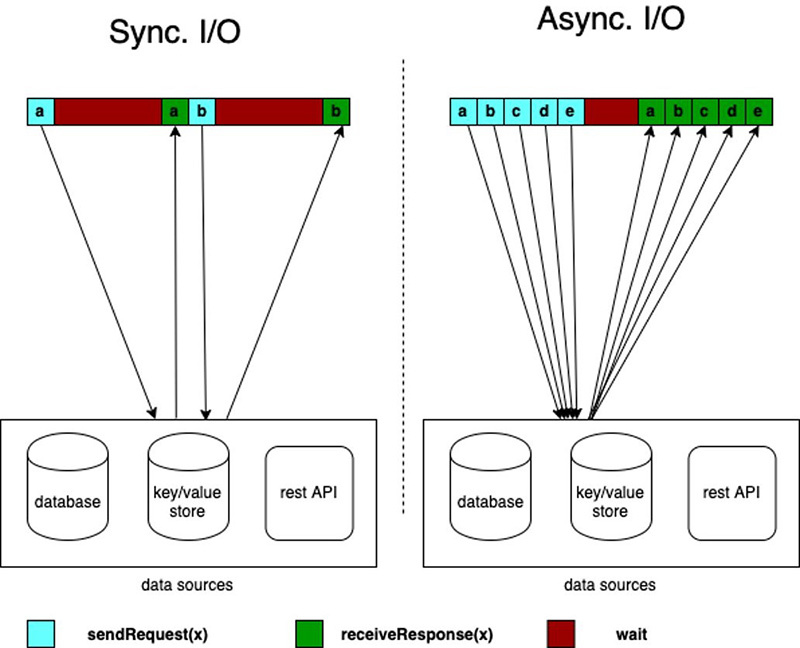
Before version 1.19, an important limitation of SQL and the Table API, compared to the Java DataStream API, was the lack of asynchronous I/O support. Any request to an external system, for example a database or a REST API, or even any AWS API call, using the AWS SDK, is synchronous and blocking. An Apache Flink’s subtask waits for the response before completing the processing of a record and proceeding to the next one. Practically, the roundtrip latency of each request was added to the processing latency for each processed record. Apache Flink’s Async I/O API removes this limitation, but it’s only available for the DataStream API and Java. Until version 1.19, there was no simple efficient workaround in SQL, the Table API, or Python.

Apache Flink 1.19 introduces the new AsyncScalarFunction, a user-defined function (UDF) that can be implemented using non-blocking calls to the external system, to support use cases similar to asynchronous I/O in SQL and the Table API.

This new type of UDF is only available in streaming mode. At the moment, it only supports ordered output. DataStream Async I/O also supports unordered output, which may further reduce latency when strict ordering isn’t required.

Python 3.11 support

Python 3.11 is now supported, and Python 3.7 support has been completely removed (FLINK-33029). Managed Service for Apache Flink currently uses the Python 3.11 runtime to run PyFlink applications. Python 3.11 is a bugfix only version of the runtime. Python 3.11 introduced several performance improvements and bug fixes, but no API breaking changes.

Performance improvements: Dynamic checkpoint interval

In the latest release of Apache Flink 1.19, significant enhancements have been made to improve checkpoint behavior. With this new release, it gives the application the capability to adjust checkpointing intervals dynamically based on whether the source is processing backlog data (FLIP-309).

In Apache Flink 1.19, you can now specify different checkpointing intervals based on whether a source operator is processing backlog data. This flexibility optimizes job performance by reducing checkpoint frequency during backlog phases, enhancing overall throughput. Extending checkpoint intervals allows Apache Flink to prioritize processing throughput over frequent state snapshots, thereby improving efficiency and performance.

To enable it, you need to define the execution.checkpointing.interval parameter for regular intervals and execution.checkpointing.interval-during-backlog to specify a longer interval when sources report processing backlog.

For example, if you want to run checkpoints every 60 seconds during normal processing, but extend to 10 minutes during the processing of backlogs, you can set the following:

  • execution.checkpointing.interval = 60s
  • execution.checkpointing.interval-during-backlog = 10m

In Amazon Managed Service for Apache Flink, the default checkpointing interval is configured by the application configuration (60 seconds by default). You don’t need to set the configuration parameter. To set a longer checkpointing interval during backlog processing, you can raise a support case to modify execution.checkpointing.interval-during-backlog. See Modifiable Flink configuration properties for further details about modifying Apache Flink configurations.

At the time of writing, dynamic checkpointing intervals are only supported by Apache Kafka source and FileSystem source connectors. If you use any other source connector, intervals during backlog are ignored, and Apache Flink runs a checkpoint at the default interval during backlog processing.

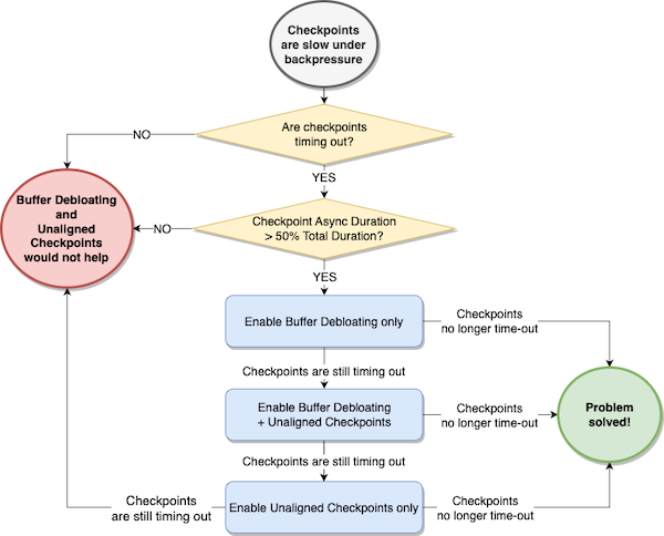
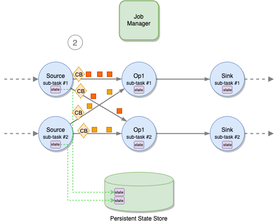
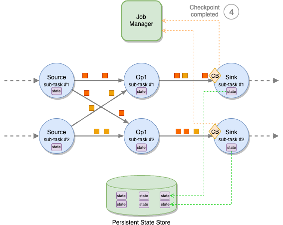
In Apache Flink, checkpoints are always injected in the flow from the sources. This feature only involves source connectors. The sink connectors you use in your application don’t affect this feature. For a deep dive into the Apache Flink checkpoint mechanism, see Optimize checkpointing in your Amazon Managed Service for Apache Flink applications with buffer debloating and unaligned checkpoints.

More troubleshooting information: Job initialization and checkpoint traces

With FLIP-384, Apache Flink 1.19 introduces trace reporters, which show checkpointing and job initialization traces. As of 1.19, this trace information can be sent to the logs using Slf4j. In Managed Service for Apache Flink, this is now enabled by default. You can find checkpoint and job initialization details in Amazon CloudWatch Logs, with the other logs from the application.

Checkpoint traces contain valuable information about each checkpoint. You can find similar information on the Apache Flink Dashboard, but only for the latest checkpoints and only while the application is running. Conversely, in the logs, you can find the full history of checkpoints. The following is an example of a checkpoint trace:

SimpleSpan{
  scope=org.apache.flink.runtime.checkpoint.CheckpointStatsTracker, 
  name=Checkpoint, 
  startTsMillis=1718779769305, 
  endTsMillis=1718779769542, 
  attributes={
    jobId=1b418a2404cbcf47ef89071f83f2dff9, 
    checkpointId=9774, 
    checkpointStatus=COMPLETED, 
    fullSize=9585, 
    checkpointedSize=9585
  }
}

Job initialization traces are generated when the job starts and recovers the state from a checkpoint or savepoint. You can find valuable statistics you can’t normally find elsewhere, including the Apache Flink Dashboard. The following is an example of a job initialization trace:

SimpleSpan{
  scope=org.apache.flink.runtime.checkpoint.CheckpointStatsTracker,
  name=JobInitialization,
  startTsMillis=1718781201463,
  endTsMillis=1718781409657,
  attributes={
    maxReadOutputDataDurationMs=89,
    initializationStatus=COMPLETED,
    fullSize=26167879378,
    sumMailboxStartDurationMs=621,
    sumGateRestoreDurationMs=29,
    sumDownloadStateDurationMs=199482,
    sumRestoredStateSizeBytes.LOCAL_MEMORY=46764,
    checkpointId=270,
    sumRestoredStateSizeBytes.REMOTE=26167832614,
    maxDownloadStateDurationMs=199482,
    sumReadOutputDataDurationMs=90,
    maxRestoredStateSizeBytes.REMOTE=26167832614,
    maxInitializeStateDurationMs=201122,
    sumInitializeStateDurationMs=201241,
    jobId=8edb291c9f1c91c088db51b48de42308,
    maxGateRestoreDurationMs=22,
    maxMailboxStartDurationMs=391,
    maxRestoredStateSizeBytes.LOCAL_MEMORY=46764
  }
}

Checkpoint and job initialization traces are logged at INFO level. You can find them in CloudWatch Logs only if you configure a logging level of INFO or DEBUG in your Managed Service for Apache Flink application.

Managed Service for Apache Flink behavior change

As a fully managed service, Managed Service for Apache Flink controls some runtime configuration parameters to guarantee the stability of your application. For details about the Apache Flink settings that can be modified, see Apache Flink settings.

With the 1.19 runtime, if you programmatically modify a configuration parameter that is directly controlled by Managed Service for Apache Flink, you receive an explicit ProgramInvocationException when the application starts, explaining what parameter is causing the problem and preventing the application from starting. With runtime 1.18 or earlier, changes to parameters controlled by the managed service were silently ignored.

To learn more about how Managed Service for Apache Flink handles configuration changes in runtime 1.19 or later, refer to FlinkRuntimeException: “Not allowed configuration change(s) were detected”.

Conclusion

In this post, we explored some of the new relevant features and configuration changes introduced with Apache Flink 1.19, now supported by Managed Service for Apache Flink. This latest version brings numerous enhancements aimed at improving performance, flexibility, and usability for developers working with Apache Flink.

With the support of Apache Flink 1.19, Managed Service for Apache Flink now supports the latest released Apache Flink version. We have seen some of the interesting new features available for Flink SQL and PyFlink.

You can find more details about recent releases from the Apache Flink blog and release notes:

If you’re new to Apache Flink, we recommend our guide to choosing the right API and language and following the getting started guide to start using Managed Service for Apache Flink.

If you’re already running an application in Managed Service for Apache Flink, you can safely upgrade it in-place to the new 1.19 runtime.


About the Authors

Francisco Morillo is a Streaming Solutions Architect at AWS, specializing in real-time analytics architectures. With over five years in the streaming data space, Francisco has worked as a data analyst for startups and as a big data engineer for consultancies, building streaming data pipelines. He has deep expertise in Amazon Managed Streaming for Apache Kafka (Amazon MSK) and Amazon Managed Service for Apache Flink. Francisco collaborates closely with AWS customers to build scalable streaming data solutions and advanced streaming data lakes, ensuring seamless data processing and real-time insights.

Lorenzo Nicora works as Senior Streaming Solution Architect at AWS, helping customers across EMEA. He has been building cloud-centered, data-intensive systems for over 25 years, working in the finance industry both through consultancies and for FinTech product companies. He has leveraged open-source technologies extensively and contributed to several projects, including Apache Flink.

Build a real-time streaming generative AI application using Amazon Bedrock, Amazon Managed Service for Apache Flink, and Amazon Kinesis Data Streams

Post Syndicated from Felix John original https://aws.amazon.com/blogs/big-data/build-a-real-time-streaming-generative-ai-application-using-amazon-bedrock-amazon-managed-service-for-apache-flink-and-amazon-kinesis-data-streams/

Generative artificial intelligence (AI) has gained a lot of traction in 2024, especially around large language models (LLMs) that enable intelligent chatbot solutions. Amazon Bedrock is a fully managed service that offers a choice of high-performing foundation models (FMs) from leading AI companies such as AI21 Labs, Anthropic, Cohere, Meta, Mistral AI, Stability AI, and Amazon through a single API, along with a broad set of capabilities to help you build generative AI applications with security, privacy, and responsible AI. Use cases around generative AI are vast and go well beyond chatbot applications; for instance, generative AI can be used for analysis of input data such as sentiment analysis of reviews.

Most businesses generate data continuously in real-time. Internet of Things (IoT) sensor data, application log data from your applications, or clickstream data generated by users of your website are only some examples of continuously generated data. In many situations, the ability to process this data quickly (in real-time or near real-time) helps businesses increase the value of insights they get from their data.

One option to process data in real-time is using stream processing frameworks such as Apache Flink. Flink is a framework and distributed processing engine for processing data streams. AWS provides a fully managed service for Apache Flink through Amazon Managed Service for Apache Flink, which enables you to build and deploy sophisticated streaming applications without setting up infrastructure and managing resources.

Data streaming enables generative AI to take advantage of real-time data and provide businesses with rapid insights. This post looks at how to integrate generative AI capabilities when implementing a streaming architecture on AWS using managed services such as Managed Service for Apache Flink and Amazon Kinesis Data Streams for processing streaming data and Amazon Bedrock to utilize generative AI capabilities. We focus on the use case of deriving review sentiment in real-time from customer reviews in online shops. We include a reference architecture and a step-by-step guide on infrastructure setup and sample code for implementing the solution with the AWS Cloud Development Kit (AWS CDK). You can find the code to try it out yourself on the GitHub repo.

Solution overview

The following diagram illustrates the solution architecture. The architecture diagram depicts the real-time streaming pipeline in the upper half and the details on how you gain access to the Amazon OpenSearch Service dashboard in the lower half.

Architecture Overview

The real-time streaming pipeline consists of a producer that is simulated by running a Python script locally that is sending reviews to a Kinesis Data Stream. The reviews are from the Large Movie Review Dataset and contain positive or negative sentiment. The next step is the ingestion to the Managed Service for Apache Flink application. From within Flink, we are asynchronously calling Amazon Bedrock (using Anthropic Claude 3 Haiku) to process the review data. The results are then ingested into an OpenSearch Service cluster for visualization with OpenSearch Dashboards. We directly call the PutRecords API of Kinesis Data Streams within the Python script for the sake of simplicity and to cost-effectively run this example. You should consider using an Amazon API Gateway REST API as a proxy in front of Kinesis Data Streams when using a similar architecture in production, as described in Streaming Data Solution for Amazon Kinesis.

To gain access to the OpenSearch dashboard, we need to use a bastion host that is deployed in the same private subnet within your virtual private cloud (VPC) as your OpenSearch Service cluster. To connect with the bastion host, we use Session Manager, a capability of Amazon Systems Manager, which allows us to connect to our bastion host securely without having to open inbound ports. To access it, we use Session Manager to port forward the OpenSearch dashboard to our localhost.

The walkthrough consists of the following high-level steps:

  1. Create the Flink application by building the JAR file.
  2. Deploy the AWS CDK stack.
  3. Set up and connect to OpenSearch Dashboards.
  4. Set up the streaming producer.

Prerequisites

For this walkthrough, you should have the following prerequisites:

Implementation details

This section focuses on the Flink application code of this solution. You can find the code on GitHub. The StreamingJob.java file inside the flink-async-bedrock directory file serves as entry point to the application. The application uses the FlinkKinesisConsumer, which is a connector for reading streaming data from a Kinesis Data Stream. It applies a map transformation to convert each input string into an instance of Review class object, resulting in DataStream<Review> to ease processing.

The Flink application uses the helper class AsyncDataStream defined in the StreamingJob.java file to incorporate an asynchronous, external operation into Flink. More specifically, the following code creates an asynchronous data stream by applying the AsyncBedrockRequest function to each element in the inputReviewStream. The application uses unorderedWait to increase throughput and reduce idle time because event ordering is not required. The timeout is set to 25,000 milliseconds to give the Amazon Bedrock API enough time to process long reviews. The maximum concurrency or capacity is limited to 1,000 requests at a time. See the following code:

DataStream<ProcessedReview> processedReviewStream = AsyncDataStream.unorderedWait(inputReviewStream, new AsyncBedrockRequest(applicationProperties), 25000, TimeUnit.MILLISECONDS, 1000).uid("processedReviewStream");

The Flink application initiates asynchronous calls to the Amazon Bedrock API, invoking the Anthropic Claude 3 Haiku foundation model for each incoming event. We use Anthropic Claude 3 Haiku on Amazon Bedrock because it is Anthropic’s fastest and most compact model for near-instant responsiveness. The following code snippet is part of the AsyncBedrockRequest.java file and illustrates how we set up the required configuration to call the Anthropic’s Claude Messages API to invoke the model:

@Override
public void asyncInvoke(Review review, final ResultFuture<ProcessedReview> resultFuture) throws Exception {

    // [..]

    JSONObject user_message = new JSONObject()
        .put("role", "user")
        .put("content", "<review>" + reviewText + "</review>");

    JSONObject assistant_message = new JSONObject()
        .put("role", "assistant")
        .put("content", "{");

    JSONArray messages = new JSONArray()
            .put(user_message)
            .put(assistant_message);

    String payload = new JSONObject()
            .put("system", systemPrompt)
            .put("anthropic_version", "bedrock-2023-05-31")
            .put("temperature", 0.0)
            .put("max_tokens", 4096)
            .put("messages", messages)
            .toString();

    InvokeModelRequest request = InvokeModelRequest.builder()
            .body(SdkBytes.fromUtf8String(payload))
            .modelId("anthropic.claude-3-haiku-20240307-v1:0")
            .build();

    CompletableFuture<InvokeModelResponse> completableFuture = client.invokeModel(request)
            .whenComplete((response, exception) -> {
                if (exception != null) {
                    LOG.error("Model invocation failed: " + exception);
                }
            })
            .orTimeout(250000, TimeUnit.MILLISECONDS);

Prompt engineering

The application uses advanced prompt engineering techniques to guide the generative AI model’s responses and provide consistent responses. The following prompt is designed to extract a summary as well as a sentiment from a single review:

String systemPrompt = 
     "Summarize the review within the <review> tags 
     into a single and concise sentence alongside the sentiment 
     that is either positive or negative. Return a valid JSON object with 
     following keys: summary, sentiment. 
     <example> {\\\"summary\\\": \\\"The reviewer strongly dislikes the movie, 
     finding it unrealistic, preachy, and extremely boring to watch.\\\", 
     \\\"sentiment\\\": \\\"negative\\\"} 
     </example>";

The prompt instructs the Anthropic Claude model to return the extracted sentiment and summary in JSON format. To maintain consistent and well-structured output by the generative AI model, the prompt uses various prompt engineering techniques to improve the output. For example, the prompt uses XML tags to provide a clearer structure for Anthropic Claude. Moreover, the prompt contains an example to enhance Anthropic Claude’s performance and guide it to produce the desired output. In addition, the prompt pre-fills Anthropic Claude’s response by pre-filling the Assistant message. This technique helps provide a consistent output format. See the following code:

JSONObject assistant_message = new JSONObject()
    .put("role", "assistant")
    .put("content", "{");

Build the Flink application

The first step is to download the repository and build the JAR file of the Flink application. Complete the following steps:

  1. Clone the repository to your desired workspace:
    git clone https://github.com/aws-samples/aws-streaming-generative-ai-application.git

  2. Move to the correct directory inside the downloaded repository and build the Flink application:
    cd flink-async-bedrock && mvn clean package

Building Jar File

Maven will compile the Java source code and package it in a distributable JAR format in the directory flink-async-bedrock/target/ named flink-async-bedrock-0.1.jar. After you deploy your AWS CDK stack, the JAR file will be uploaded to Amazon Simple Storage Service (Amazon S3) to create your Managed Service for Apache Flink application.

Deploy the AWS CDK stack

After you build the Flink application, you can deploy your AWS CDK stack and create the required resources:

  1. Move to the correct directory cdk and deploy the stack:
    cd cdk && npm install & cdk deploy

This will create the required resources in your AWS account, including the Managed Service for Apache Flink application, Kinesis Data Stream, OpenSearch Service cluster, and bastion host to quickly connect to OpenSearch Dashboards, deployed in a private subnet within your VPC.

  1. Take note of the output values. The output will look similar to the following:
 ✅  StreamingGenerativeAIStack

✨  Deployment time: 1414.26s

Outputs:
StreamingGenerativeAIStack.BastionHostBastionHostIdC743CBD6 = i-0970816fa778f9821
StreamingGenerativeAIStack.accessOpenSearchClusterOutput = aws ssm start-session --target i-0970816fa778f9821 --document-name AWS-StartPortForwardingSessionToRemoteHost --parameters '{"portNumber":["443"],"localPortNumber":["8157"], "host":["vpc-generative-ai-opensearch-qfssmne2lwpzpzheoue7rkylmi.us-east-1.es.amazonaws.com"]}'
StreamingGenerativeAIStack.bastionHostIdOutput = i-0970816fa778f9821
StreamingGenerativeAIStack.domainEndpoint = vpc-generative-ai-opensearch-qfssmne2lwpzpzheoue7rkylmi.us-east-1.es.amazonaws.com
StreamingGenerativeAIStack.regionOutput = us-east-1
Stack ARN:
arn:aws:cloudformation:us-east-1:<AWS Account ID>:stack/StreamingGenerativeAIStack/3dec75f0-cc9e-11ee-9b16-12348a4fbf87

✨  Total time: 1418.61s

Set up and connect to OpenSearch Dashboards

Next, you can set up and connect to OpenSearch Dashboards. This is where the Flink application will write the extracted sentiment as well as the summary from the processed review stream. Complete the following steps:

  1. Run the following command to establish connection to OpenSearch from your local workspace in a separate terminal window. The command can be found as output named accessOpenSearchClusterOutput.
    • For Mac/Linux, use the following command:
aws ssm start-session --target <BastionHostId> --document-name AWS-StartPortForwardingSessionToRemoteHost --parameters '{"portNumber":["443"],"localPortNumber":["8157"], "host":["<OpenSearchDomainHost>"]}'
    • For Windows, use the following command:
aws ssm start-session ^
    —target <BastionHostId> ^
    —document-name AWS-StartPortForwardingSessionToRemoteHost ^    
    —parameters host="<OpenSearchDomainHost>",portNumber="443",localPortNumber="8157"

It should look similar to the following output:

Session Manager CLI

  1. Create the required index in OpenSearch by issuing the following command:
    • For Mac/Linux, use the following command:
curl --location -k --request PUT https://localhost:8157/processed_reviews \
--header 'Content-Type: application/json' \
--data-raw '{
  "mappings": {
    "properties": {
        "reviewId": {"type": "integer"},
        "userId": {"type": "keyword"},
        "summary": {"type": "keyword"},
        "sentiment": {"type": "keyword"},
        "dateTime": {"type": "date"}}}}}'
    • For Windows, use the following command:
$url = https://localhost:8157/processed_reviews
$headers = @{
    "Content-Type" = "application/json"
}
$body = @{
    "mappings" = @{
        "properties" = @{
            "reviewId" = @{ "type" = "integer" }
            "userId" = @{ "type" = "keyword" }
            "summary" = @{ "type" = "keyword" }
            "sentiment" = @{ "type" = "keyword" }
            "dateTime" = @{ "type" = "date" }
        }
    }
} | ConvertTo-Json -Depth 3
Invoke-RestMethod -Method Put -Uri $url -Headers $headers -Body $body -SkipCertificateCheck
  1. After the session is established, you can open your browser and navigate to https://localhost:8157/_dashboards. Your browser might consider the URL not secure. You can ignore this warning.
  2. Choose Dashboards Management under Management in the navigation pane.
  3. Choose Saved objects in the sidebar.
  4. Import export.ndjson, which can be found in the resources folder within the downloaded repository.

OpenSearch Dashboards Upload

  1. After you import the saved objects, you can navigate to Dashboards under My Dashboard in the navigation pane.

At the moment, the dashboard appears blank because you haven’t uploaded any review data to OpenSearch yet.

Set up the streaming producer

Finally, you can set up the producer that will be streaming review data to the Kinesis Data Stream and ultimately to the OpenSearch Dashboards. The Large Movie Review Dataset was originally published in 2011 in the paper “Learning Word Vectors for Sentiment Analysis” by Andrew L. Maas, Raymond E. Daly, Peter T. Pham, Dan Huang, Andrew Y. Ng, and Christopher Potts. Complete the following steps:

  1. Download the Large Movie Review Dataset here.
  2. After the download is complete, extract the .tar.gz file to retrieve the folder named aclImdb 3 or similar that contains the review data. Rename the review data folder to aclImdb.
  3. Move the extracted dataset to data/ inside the repository that you previously downloaded.

Your repository should look like the following screenshot.

Folder Overview

  1. Modify the DATA_DIR path in producer/producer.py if the review data is named differently.
  2. Move to the producer directory using the following command:
    cd producer

  3. Install the required dependencies and start generating the data:
    pip install -r requirements.txt && python produce.py

The OpenSearch dashboard should be populated after you start generating streaming data and writing it to the Kinesis Data Stream. Refresh the dashboard to view the latest data. The dashboard shows the total number of processed reviews, the sentiment distribution of the processed reviews in a pie chart, and the summary and sentiment for the latest reviews that have been processed.

When you have a closer look at the Flink application, you will notice that the application marks the sentiment field with the value error whenever there is an error with the asynchronous call made by Flink to the Amazon Bedrock API. The Flink application simply filters the correctly processed reviews and writes them to the OpenSearch dashboard.

For robust error handling, you should write any incorrectly processed reviews to a separate output stream and not discard them completely. This separation allows you to handle failed reviews differently than successful ones for simpler reprocessing, analysis, and troubleshooting.

Clean up

When you’re done with the resources you created, complete the following steps:

  1. Delete the Python producer using Ctrl/Command + C.
  2. Destroy your AWS CDK stack by returning to the root folder and running the following command in your terminal:
    cd cdk && cdk destroy

  3. When asked to confirm the deletion of the stack, enter yes.

Conclusion

In this post, you learned how to incorporate generative AI capabilities in your streaming architecture using Amazon Bedrock and Managed Service for Apache Flink using asynchronous requests. We also gave guidance on prompt engineering to derive the sentiment from text data using generative AI. You can build this architecture by deploying the sample code from the GitHub repository.

For more information on how to get started with Managed Service for Apache Flink, refer to Getting started with Amazon Managed Service for Apache Flink (DataStream API). For details on how to set up Amazon Bedrock, refer to Set up Amazon Bedrock. For other posts on Managed Service for Apache Flink, browse through the AWS Big Data Blog.


About the Authors

Felix John is a Solutions Architect and data streaming expert at AWS, based in Germany. He focuses on supporting small and medium businesses on their cloud journey. Outside of his professional life, Felix enjoys playing Floorball and hiking in the mountains.

Michelle Mei-Li Pfister is a Solutions Architect at AWS. She is supporting customers in retail and consumer packaged goods (CPG) industry on their cloud journey. She is passionate about topics around data and machine learning.

Uncover social media insights in real time using Amazon Managed Service for Apache Flink and Amazon Bedrock

Post Syndicated from Francisco Morillo original https://aws.amazon.com/blogs/big-data/uncover-social-media-insights-in-real-time-using-amazon-managed-service-for-apache-flink-and-amazon-bedrock/

With over 550 million active users, X (formerly known as Twitter) has become a useful tool for understanding public opinion, identifying sentiment, and spotting emerging trends. In an environment where over 500 million tweets are sent each day, it’s crucial for brands to effectively analyze and interpret the data to maximize their return on investment (ROI), which is where real-time insights play an essential role.

Amazon Managed Service for Apache Flink helps you to transform and analyze streaming data in real time with Apache Flink. Apache Flink supports stateful computation over a large volume of data in real time with exactly-once consistency guarantees. Moreover, Apache Flink’s support for fine-grained control of time with highly customizable window logic enables the implementation of the advanced business logic required for building a streaming data platform. Stream processing and generative artificial intelligence (AI) have emerged as powerful tools to harness the potential of real time data. Amazon Bedrock, along with foundation models (FMs) such as Anthropic Claude on Amazon Bedrock, empowers a new wave of AI adoption by enabling natural language conversational experiences.

In this post, we explore how to combine real-time analytics with the capabilities of generative AI and use state-of-the-art natural language processing (NLP) models to analyze tweets through queries related to your brand, product, or topic of choice. It goes beyond basic sentiment analysis and allows companies to provide actionable insights that can be used immediately to enhance customer experience. These include:

  • Identifying rising trends and discussion topics related to your brand
  • Conducting granular sentiment analysis to truly understand customers’ opinions
  • Detecting nuances such as emojis, acronyms, sarcasm, and irony
  • Spotting and addressing concerns proactively before they spread
  • Guiding product development based on feature requests and feedback
  • Creating targeted customer segments for information campaigns

This post takes a step-by-step approach to showcase how you can use Retrieval Augmented Generation (RAG) to reference real-time tweets as a context for large language models (LLMs). RAG is the process of optimizing the output of an LLM so it references an authoritative knowledge base outside of its training data sources before generating a response. LLMs are trained on vast volumes of data and use billions of parameters to generate original output for tasks such as answering questions, translating languages, and completing sentences. RAG extends the already powerful capabilities of LLMs to specific domains or an organization’s internal knowledge base, all without the need to retrain the model. It’s a cost-effective approach to improving LLM output so it remains relevant, accurate, and useful in various contexts.

Solution overview

In this section, we explain the flow and architecture of the application. We divide the flow of the application into two parts:

  • Data ingestion – Ingest data from streaming sources, convert it to vector embeddings, and then store them in a vector database
  • Insights retrieval – Invoke an LLM with the user queries to retrieve insights on tweets using the RAG technique

Data ingestion

The following diagram describes the data ingestion flow:

  1. Process feeds from streaming sources, such as social media feeds, Amazon Kinesis Data Streams, or Amazon Managed Service for Apache Kafka (Amazon MSK).
  2. Convert streaming data to vector embeddings in real time.
  3. Store them in a vector database.

Data is ingested from a streaming source (for example, X) and processed using an Apache Flink application. Apache Flink is an open source stream processing framework. It provides powerful streaming capabilities, enabling real-time processing, stateful computations, fault tolerance, high throughput, and low latency. Apache Flink is used to process the streaming data, perform deduplication, and invoke an embedding model to create vector embeddings.

Vector embeddings are numerical representations that capture the relationships and meaning of words, sentences, and other data types. These vector embeddings will be used for semantic search or neural search to retrieve relevant information that will be used as context for the LLM to evaluate the response. After the text data is converted into vectors, the vectors are persisted in an Amazon OpenSearch Service domain, which will be used as a vector database. Unlike traditional relational databases with rows and columns, data points in a vector database are represented by vectors with a fixed number of dimensions, which are clustered based on similarity.

OpenSearch Service offers scalable and efficient similarity search capabilities tailored for handling large volumes of dense vector data. OpenSearch Service seamlessly integrates with other AWS services, enabling you to build robust data pipelines within AWS. As a fully managed service, OpenSearch Service alleviates the operational overhead of managing the underlying infrastructure, while providing essential features like approximate k-Nearest Neighbor (k-NN) search algorithms, dense vector support, and robust monitoring and logging tools through Amazon CloudWatch. These capabilities make OpenSearch Service a suitable solution for applications that require fast and accurate similarity-based retrieval tasks using vector embeddings.

This design enables real-time vector embedding, making it ideal for AI-driven applications.

Insights retrieval

The following diagram shows the flow from the user side, where the user places a query through the frontend and gets a response from the LLM model using the retrieved vector database documents as the context provided in the prompt.

As shown in the preceding figure, to retrieve insights from the LLM, first you need to receive a query from the user. The text query is then converted into vector embeddings using the same model that was used before for the tweets. It’s important to make sure the same embedding model is used for both ingestion and search. The vector embeddings are then used to perform a semantic search in the vector database to obtain the related vectors and associated text. This serves as the context for the prompt. Next, the previous conversation history (if any) is added to the prompt. This serves as the conversation history for the model. Finally, the user’s question is also included in the prompt and the LLM is invoked to get the response.

For the purpose of this post, we don’t take into consideration the conversation history or store it for later use.

Solution architecture

Now that you understand the overall process flow, let’s analyze the following architecture using AWS services step by step.

The first part of the preceding figure shows the data ingestion process:

  1. A user authenticates with Amazon Cognito.
  2. The user connects to the Streamlit frontend and configures the following parameters: query terms, API bearer token, and frequency to retrieve tweets.
  3. Managed Service for Apache Flink is used to consume and process the tweets in real time and stores in Apache Flink’s state the parameters for making the API requests received from the frontend application.
  4. The streaming application uses Apache Flink’s async I/O to invoke the Amazon Titan Embeddings model through the Amazon Bedrock API.
  5. Amazon Bedrock returns a vector embedding for each tweet.
  6. The Apache Flink application then writes the vector embedding with the original text of the tweet into an OpenSearch Service k-NN index.

The remainder of the architecture diagram shows the insights retrieval process:

  1. A user sends a query through the Streamlit frontend application.
  2. An AWS Lambda function is invoked by Amazon API Gateway, passing the user query as input.
  3. The Lambda function uses LangChain to orchestrate the RAG process. As a first step, the function invokes the Amazon Titan Embeddings model on Amazon Bedrock to create a vector embedding for the question.
  4. Amazon Bedrock returns the vector embedding for the question.
  5. As a second step in the RAG orchestration process, the Lambda function performs a semantic search in OpenSearch Service and retrieves the relevant documents related to the question.
  6. OpenSearch Service returns the relevant documents containing the tweet text to the Lambda function.
  7. As a last step in the LangChain orchestration process, the Lambda function augments the prompt, adding the context and using few-shot prompting. The augmented prompt, including instructions, examples, context, and query, is sent to the Anthropic Claude model through the Amazon Bedrock API.
  8. Amazon Bedrock returns the answer to the question in natural language to the Lambda function.
  9. The response is sent back to the user through API Gateway.
  10. API Gateway provides the response to the user question in the Streamlit application.

The solution is available in the GitHub repo. Follow the README file to deploy the solution.

Now that you understand the overall flow and architecture, let’s dive deeper into some of the key steps to understand how it works.

Amazon Bedrock chatbot UI

The Amazon Bedrock chatbot Streamlit application is designed to provide insights from tweets, whether they are real tweets ingested from the X API or simulated tweets or messages from the My Social Media application.

In the Streamlit application, we can provide the parameters that will be used to make the API requests to the X Developer API and pull the data from X. We developed an Apache Flink application that adjusts the API requests based on the provided parameters.

As parameters, you need to provide the following:

  • Bearer token for API authorization – This is obtained from the X Developer platform when you sign up to use the APIs.
  • Query terms to be used to filter the tweets consumed – You can use the search operators available in the X documentation.
  • Frequency of the request – The X basic API only allows you to make a request every 15 seconds. If a lower interval is set, the application won’t pull data.

The parameters are sent to Kinesis Data Streams through API Gateway and are consumed by the Apache Flink application.

My Social Media UI

The My Social Media application is a Streamlit application that serves as an additional UI. Through this application, users can compose and send messages, simulating the experience of posting on a social media site. These messages are then ingested into an AWS data pipeline consisting of API Gateway, Kinesis Data Streams, and an Apache Flink application. The Apache Flink application processes the incoming messages, invokes an Amazon Bedrock embedding model, and stores the data in an OpenSearch Service cluster.

To accommodate both real X data and simulated data from the My Social Media application, we’ve set up separate indexes within the OpenSearch Service cluster. This separation allows users to choose which data source they want to analyze or query. The Streamlit application features a sidebar option called Use X Index that acts as a toggle. When this option is enabled, the application queries and analyzes data from the index containing real tweets ingested from the X API. If the option is disabled, the application queries and displays data from the index containing messages sent through the My Social Media application.

Apache Flink is used because of its ability to scale with the increasing volume of tweets. The Apache Flink application is responsible for performing data ingestion as explained previously. Let’s dive into the details of the flow.

Consume data from X

We use Apache Flink to process the API parameters sent from the Streamlit UI. We store the parameters in Apache Flink’s state, which allows us to modify and update the parameters without having to restart the application. We use the ProcessFunction to use Apache Flink’s internal timers to schedule the frequency of requests to fetch tweets. In this post, we use X’s Recent search API, which allows us to access filtered public tweets posted over the last 7 days. The API response is paginated and returns a maximum of 100 tweets on each request in reverse chronological order. If there are more tweets to be consumed, the response of the previous request will return a token, which needs to be used in the next API call. After we receive the tweets from the API, we apply the following transformations:

  • Filter out the empty tweets (tweets without any text).
  • Partition the set of tweets by author ID. This helps distribute the processing to multiple subtasks in Apache Flink.
  • Apply a deduplication logic to only process tweets that haven’t been processed. For this, we store the already processed tweet ID in Apache Flink’s state and match and filter out the tweets that have already been processed. We store the tweets’ ID grouped by author ID, which can cause the state size of the application to increase. Because the API only provides tweets from the last 7 days when invoked, we have introduced a time-to-live (TTL) of 7 days so we don’t grow the application’s state indefinitely. You can modify this based on your requirements.
  • Convert tweets into JSON objects for a later Amazon Bedrock API invocation.

Create vector embeddings

The vector embeddings are created by invoking the Amazon Titan Embeddings model through the Amazon Bedrock API. Asynchronous invocations of external APIs are important performance considerations when building a stream processing architecture. Synchronous calls increase latency, reduce throughput, and can be a bottleneck for overall processing.

To invoke the Amazon Bedrock API, you will use the Amazon Bedrock Runtime dependency in Java, which provides an asynchronous client that allows us invoke Amazon Bedrock models asynchronously through the BedrockRuntimeAsyncClient. This is invoked to create the embeddings. For this we use Apache Flink’s async I/O to make asynchronous requests to external APIs. Apache Flink’s async I/O is a library within Apache Flink that allows you to write asynchronous, non-blocking operators for stream processing applications, enabling better utilization of resources and higher throughput. We provide the asynchronous function to be called, the timeout duration that determines how long an asynchronous operation can take before it’s considered failed, and the maximum number of requests that should be in progress at any point in time. Limiting the number of concurrent requests makes sure that the operator won’t accumulate an ever-growing backlog of pending requests. However, this can cause backpressure after the capacity is exhausted. Because we use the timestamp of creation when we ingest into OpenSearch Service and so order won’t affect our results, we can use Apache Flink’s async I/O unordered function, allowing us to have better throughput and performance. See the following code:

DataStream<JSONObject> resultStream = AsyncDataStream

.unorderedWait(inputJSON, new BedRockEmbeddingModelAsyncTweetFunction(), 15000, TimeUnit.MILLISECONDS, 1000)
.uid("tweet-async-function");

Let’s have a closer look into the Apache Flink async I/O function. The following is within the CompletableFuture Java class:

  1. First, we create the Amazon Bedrock Runtime async client:
BedrockRuntimeAsyncClient runtime = BedrockRuntimeAsyncClient.builder()
.region(Region.of(region))  // Use the specified AWS region 
.build();
  1. We then extract the tweet for the event and build the payload that we will send to Amazon Bedrock:
String stringBody = jsonObject.getString("tweet");

ArrayList<String> stringList = new ArrayList<>();


stringList.add(stringBody);


JSONObject jsonBody = new JSONObject()
.put("inputText", stringBody);


SdkBytes body = SdkBytes.fromUtf8String(jsonBody.toString());
  1. After we have the payload, we can call the InvokeModel API and invoke Amazon Titan to create the vector embeddings for the tweets:
InvokeModelRequest request = InvokeModelRequest.builder()
        
.modelId("amazon.titan-embed-text-v1")
        
.contentType("application/json")
        
.accept("*/*")
        
.body(body)
        
.build();

CompletableFuture<InvokeModelResponse> futureResponse = runtime.invokeModel(request);
  1. After receiving the vector, we append the following fields to the output JSONObject:
    1. Cleaned tweet
    2. Tweet creation timestamp
    3. Number of likes of the tweet
    4. Number of retweets
    5. Number of views from the tweet (impressions)
    6. Tweet ID
// Extract and process the response when it is available
JSONObject response = new JSONObject(
        futureResponse.join().body().asString(StandardCharsets.UTF_8)
);

// Add additional fields related to tweet data to the response
response.put("tweet", jsonObject.get("tweet"));
response.put("@timestamp", jsonObject.get("created_at"));
response.put("likes", jsonObject.get("likes"));
response.put("retweet_count", jsonObject.get("retweet_count"));
response.put("impression_count", jsonObject.get("impression_count"));
response.put("_id", jsonObject.get("_id"));

return response;

This will return the embeddings, original text, additional fields, and the number of tokens used for the embedding. In our connector, we are only consuming messages in English, as well as ignoring messages that are retweets from other tweets.

The same processing steps are replicated for messages coming from the My Social Media application (manually ingested).

Store vector embeddings in OpenSearch Service

We use OpenSearch Service as a vector database for semantic search. Before we can write the data into OpenSearch Service, we need to create an index that supports semantic search. We are using the k-NN plugin. The vector database index mapping should have the following properties for storing vectors for similarity search:

"embeddings": {
        "type": "knn_vector",
        "dimension": 1536,
        "method": {
          "name": "hnsw",
          "space_type": "l2",
          "engine": "nmslib",
          "parameters": {
            "ef_construction": 128,
            "m": 24
          }
        }
      }

The key parameters are as follows:

  • type – This specifies that the field will hold vector data for a k-NN similarity search. The value should be knn_vector.
  • dimension – The number of dimensions for each vector. This must match the model dimension. In this case we use 1,536 dimensions, the same as the Amazon Titan Text Embeddings v1 model.
  • method – Defines the algorithm and parameters for indexing and searching the vectors:
    • name – The identifier for the nearest neighbor method. We use hierarchical navigable small worlds (HNSW)—a hierarchical proximity graph approach—to run a approximate k-NN (A-NN) search because standard k-NN is not a scalable approach.
    • space_type – The vector space used to calculate the distance between vectors. It supports multiple space type. The default value is 12.
    • engine – The approximate k-NN library to use for indexing and search. The available libraries are faiss, nmslib, and Lucene.
    • ef_construction – The size of the dynamic list used during k-NN graph creation. Higher values result in a more accurate graph but slower indexing speed.
    • m – The number of bidirectional links that the plugin creates for each new element. Increasing and decreasing this value can have a large impact on memory consumption. Keep this value between 2–100.

Standard k-NN search methods compute similarity using a brute-force approach that measures the nearest distance between a query and a number of points, which produces exact results. This works well for most applications. However, in the case of extremely large datasets with high dimensionality, this creates a scaling problem that reduces the efficiency of the search. The approximate k-NN search methods used by OpenSearch Service use approximate nearest neighbor (ANN) algorithms from the nmslib, faiss, and Lucene libraries to power k-NN search. These search methods employ ANN to improve search latency for large datasets. Of the three search methods the k-NN plugin provides, this method offers the best search scalability for large datasets. This approach is the preferred method when a dataset reaches hundreds of thousands of vectors. For more information about the different methods and their trade-offs, refer to Comprehensive Guide To Approximate Nearest Neighbors Algorithms.

To use the k-NN plugin’s approximate search functionality, we must first create a k-NN index with index.knn set to true:

    "settings" : {
      "index" : {
        "knn": true,
        "number_of_shards" : "5",
        "number_of_replicas" : "1"
      }
    }

After we have our indexes created, we can sink the data from our Apache Flink application into OpenSearch.

RetrievalQA using Lambda and LangChain implementation

For this part, we take an input question from the user and invoke a Lambda function. The Lambda function retrieves relevant tweets from OpenSearch Service as context and generates an answer using the LangChain RAG chain RetrievalQA. LangChain is a framework for developing applications powered by language models.

First, some setup. We instantiate the bedrock-runtime client that will allow the Lambda function to invoke the models:

bedrock_runtime = boto3.client("bedrock-runtime", "us-east-1")

embeddings = BedrockEmbeddings(model_id="amazon.titan-embed-text-v1", client=bedrock_runtime)

The BedrockEmbeddings class uses the Amazon Bedrock API to generate embeddings for the user’s input question. It strips new line characters from the text. Notice that we need to pass as an argument the instantiation of the bedrock_runtime client and the model ID for the Amazon Titan Text Embeddings v1 model.

Next, we instantiate the client for the OpenSearchVectorSeach LangChain class that will allow the Lambda function to connect to the OpenSearch Service domain and perform the semantic search against the previously indexed X embeddings. For the embedding function, we’re passing the embeddings model that we defined previously. This will be used during the LangChain orchestration process:

os_client = OpenSearchVectorSearch(
        index_name=aos_index,
        embedding_function=embeddings,
        http_auth=(os.environ['aosUser'], os.environ['aosPassword']),
        opensearch_url=os.environ['aosDomain'],
        timeout=300,
        use_ssl=True,
        verify_certs=True,
        connection_class=RequestsHttpConnection,
        )

We need to define the LLM model from Amazon Bedrock to use for text generation. The temperature is set to 0 to reduce hallucinations:

model_kwargs={"temperature": 0, "max_tokens": 4096}

llm = BedrockChat(
    model_id="anthropic.claude-3-haiku-20240307-v1:0",
    client=bedrock_runtime,
    model_kwargs=model_kwargs
)

Next, in our Lambda function, we create the prompt to instruct the model on the specific task of analyzing hundreds of tweets in the context. To normalize the output, we use a prompt engineering technique called few-shot prompting. Few-shot prompting allows language models to learn and generate responses based on a small number of examples or demonstrations provided in the prompt itself. In this approach, instead of training the model on a large dataset, we provide a few examples of the desired task or output within the prompt. These examples serve as a guide or conditioning for the model, enabling it to understand the context and the desired format or pattern of the response. When presented with a new input after the examples, the model can then generate an appropriate response by following the patterns and context established by the few-shot demonstrations in the prompt.

As part of the prompt, we then provide examples of questions and answers, so the chatbot can follow the same pattern when used (see the Lambda function to view the complete prompt):

template = """As a helpful agent that is an expert analysing tweets, please answer the question using only the provided tweets from the context in <context></context> tags. If you don't see valuable information on the tweets provided in the context in <context></context> tags, say you don't have enough tweets related to the question. Cite the relevant context you used to build your answer. Print in a bullet point list the top most influential tweets from the context at the end of the response.
    
    Find below some examples:
    <example1>
    question: 
    What are the main challenges or concerns mentioned in tweets about using Bedrock as a generative AI service on AWS, and how can they be addressed?
    
    answer:
    Based on the tweets provided in the context, the main challenges or concerns mentioned about using Bedrock as a generative AI service on AWS are:

1.	...
2.	...
3.	...
4.	...
...
    
    To address these concerns:

1.	...
2.	...
3.	...
4.	...
...

    Top tweets from context:

    [1] ...
    [2] ...
    [3] ...
    [4] ...

    </example1>
    
    <example2>
    ...
    </example2>
    
    Human: 
    
    question: {question}
    
    <context>
    {context}
    </context>
    
    Assistant:"""

    prompt = PromptTemplate(input_variables=["context","question"], template=template)

We then create the RetrievalQA LangChain chain using the prompt template, Anthropic Claude on Amazon Bedrock, and the OpenSearch Service retriever configured previously. The RetrievalQA LangChain chain will orchestrate the following RAG steps:

  • Invoke the text embedding model to create a vector for the user’s question
  • Perform a semantic search on OpenSearch Service using the vector to retrieve the relevant tweets to the user’s question (k=200)
  • Invoke the LLM model using the augmented prompt containing the prompt template, context (stuffed retrieved tweets) and question
chain = RetrievalQA.from_chain_type(
    llm=llm,
    verbose=True,
    chain_type="stuff",
    retriever=os_client.as_retriever(
        search_type="similarity",
        search_kwargs={
            "k": 200, 
            "space_type": "l2", 
            "vector_field": "embeddings", 
            "text_field": text_field
        }
    ),
    chain_type_kwargs = {"prompt": prompt}
)

Finally, we run the chain:

answer = chain.invoke({"query": message})

The response from the LLM is sent back to the user application. As shown in the following screenshot:

Considerations

You can extend the solution provided in this post. When you do, consider the following suggestions:

  • Configure index retention and rollover in OpenSearch Service to manage index lifecycle and data retention effectively
  • Incorporate chat history into the chatbot to provide richer context and improve the relevance of LLM responses
  • Add filters and hybrid search with the possibility to modify the weight given to the keyword and semantic search to enhance search on RAG
  • Modify the TTL for Apache Flink’s state to match your requirements (the solution in this post uses 7 days)
  • Enable logging to API Gateway and in the Streamlit application.

Summary

This post demonstrates how to combine real-time analytics with generative AI capabilities to analyze tweets related to a brand, product, or topic of interest. It uses Amazon Managed Service for Apache Flink to process tweets from the X API, create vector embeddings using the Amazon Titan Embeddings model on Amazon Bedrock, and store the embeddings in an OpenSearch Service index configured for vector similarity search—all these steps happen in real time.

The post also explains how users can input queries through a Streamlit frontend application, which invokes a Lambda function. This Lambda function retrieves relevant tweets from OpenSearch Service by performing semantic search on the stored embeddings using the LangChain RetrievalQA chain. As a result, it generates insightful answers using the Anthropic Claude LLM on Amazon Bedrock.

The solution enables identifying trends, conducting sentiment analysis, detecting nuances, addressing concerns, guiding product development, and creating targeted customer segments based on real-time X data.

To get started with generative AI, visit Generative AI on AWS for information about industry use cases, tools to build and scale generative AI applications, as well as the post Exploring real-time streaming for generative AI Applications for other use cases for streaming with generative AI.


About the Authors

Francisco Morillo is a Streaming Solutions Architect at AWS, specializing in real-time analytics architectures. With over five years in the streaming data space, Francisco has worked as a data analyst for startups and as a big data engineer for consultancies, building streaming data pipelines. He has deep expertise in Amazon Managed Streaming for Apache Kafka (Amazon MSK) and Amazon Managed Service for Apache Flink. Francisco collaborates closely with AWS customers to build scalable streaming data solutions and advanced streaming data lakes, ensuring seamless data processing and real-time insights.

Sergio Garcés Vitale is a Senior Solutions Architect at AWS, passionate about generative AI. With over 10 years of experience in the telecommunications industry, where he helped build data and observability platforms, Sergio now focuses on guiding Retail and CPG customers in their cloud adoption, as well as customers across all industries and sizes in implementing Artificial Intelligence use cases.

Subham Rakshit is a Streaming Specialist Solutions Architect for Analytics at AWS based in the UK. He works with customers to design and build search and streaming data platforms that help them achieve their business objective. Outside of work, he enjoys spending time solving jigsaw puzzles with his daughter.

AWS named a Leader in IDC MarketScape: Worldwide Analytic Stream Processing Software 2024 Vendor Assessment

Post Syndicated from Anna Montalat original https://aws.amazon.com/blogs/big-data/aws-named-a-leader-in-idc-marketscape-worldwide-analytic-stream-processing-software-2024-vendor-assessment/

We’re thrilled to announce that AWS has been named a Leader in the IDC MarketScape: Worldwide Analytic Stream Processing Software 2024 Vendor Assessment (doc #US51053123, March 2024).

We believe this recognition validates the power and performance of Apache Flink for real-time data processing, and how AWS is leading the way to help customers build and run fully managed Apache Flink applications. You can read the full report from IDC.

Unleashing real-time insights for your organization

Apache Flink’s robust architecture enables real-time data processing at scale, making it a favored choice among organizations for its efficiency and speed. With its advanced features for event time processing and state management, Apache Flink empowers users to build complex stream processing applications, making it indispensable for modern data-driven organizations. Managed Service for Apache Flink takes the complexity out of Apache Flink deployment and management, letting you focus on building game-changing applications. With Managed Service for Apache Flink, you can transform and analyze streaming data in real time using Apache Flink and integrate applications with other AWS services. There are no servers and clusters to manage, and there is no compute and storage infrastructure to set up. You pay only for the resources you use.

But what does this mean for your organizations and IT teams? The following are some use cases and benefits:

  • Faster insights, quicker action – Analyze data streams as they arrive, allowing you to react promptly to changing conditions and make informed decisions based on the latest information, achieving agility and competitiveness in dynamic markets.
  • Real-time fraud detection – Identify suspicious activity the moment it occurs, enabling proactive measures to protect your customers and revenue from potential financial losses, bolstering trust and security in your business operations.
  • Personalized customer interactions – Gain insights from user behavior in real time, enabling personalized experiences and the ability to proactively address potential issues before they impact customer satisfaction, fostering loyalty and enhancing brand reputation.
  • Data-driven optimization – Utilize real-time insights from sensor data and machine logs to streamline processes, identify inefficiencies, and optimize resource allocation, driving operational excellence and cost savings while maintaining peak performance.
  • Advanced AI – Continuously feed real-time data to your machine learning (ML) and generative artificial intelligence (AI) models, allowing them to adapt and personalize outputs for more relevant and impactful results.

Beyond the buzzword: Apache Flink in action

Apache Flink’s versatility extends beyond single use cases. The following are just a few examples of how our customers are taking advantage of its capabilities:

  • The National Hockey League is the second oldest of the four major professional team sports leagues in North America. Predicting events such as face-off winning probabilities during a live game is a complex task that requires processing a significant amount of quality historical data and data streams in real time. The NHL constructed the Face-off Probability model using Apache Flink. Managed Service for Apache Flink provides the underlying infrastructure for the Apache Flink applications, removing the need to self-manage an Apache Flink cluster and reducing maintenance complexity and costs.
  • Arity is a technology company focused on making transportation smarter, safer, and more useful. They transform massive amounts of data into actionable insights to help partners better predict risk and make smarter decisions in real time. Arity uses the managed ability of Managed Service for Apache Flink to transform and analyze streaming data in near real time using Apache Flink. On Managed Service for Apache Flink, Arity generates driving behavior insights based on collated driving data.
  • SOCAR is the leading Korean mobility company with strong competitiveness in car sharing. SOCAR solves mobility-related social problems, such as parking difficulties and traffic congestion, and changes the car ownership-oriented mobility habits in Korea.

Join the leaders in stream processing

By choosing Managed Service for Apache Flink, you’re joining a growing community of organizations who are unlocking the power of real-time data analysis. Get started today and see how Apache Flink can transform your data strategy, including powering the next generation of generative AI applications.

Ready to learn more?

Contact us today and discover how Apache Flink can empower your business.


About the author

Anna Montalat is the Product Marketing lead for AWS analytics and streaming data services, including Amazon Managed Streaming for Apache Kafka (MSK), Kinesis Data Streams, Kinesis Video Streams, Amazon Data Firehose, and Amazon Managed Service for Apache Flink, among others. She is passionate about bringing new and emerging technologies to market, working closely with service teams and enterprise customers. Outside of work, Anna skis through winter time and sails through summer.

In-place version upgrades for applications on Amazon Managed Service for Apache Flink now supported

Post Syndicated from Jeremy Ber original https://aws.amazon.com/blogs/big-data/in-place-version-upgrades-for-applications-on-amazon-managed-service-for-apache-flink-now-supported/

For existing users of Amazon Managed Service for Apache Flink who are excited about the recent announcement of support for Apache Flink runtime version 1.18, you can now statefully migrate your existing applications that use older versions of Apache Flink to a more recent version, including Apache Flink version 1.18. With in-place version upgrades, upgrading your application runtime version can be achieved simply, statefully, and without incurring data loss or adding additional orchestration to your workload.

Apache Flink is an open source distributed processing engine, offering powerful programming interfaces for both stream and batch processing, with first-class support for stateful processing and event time semantics. Apache Flink supports multiple programming languages, Java, Python, Scala, SQL, and multiple APIs with different level of abstraction, which can be used interchangeably in the same application.

Managed Service for Apache Flink is a fully managed, serverless experience in running Apache Flink applications, and now supports Apache Flink 1.18.1, the latest released version of Apache Flink at the time of writing.

In this post, we explore in-place version upgrades, a new feature offered by Managed Service for Apache Flink. We provide guidance on getting started and offer detailed insights into the feature. Later, we deep dive into how the feature works and some sample use cases.

This post is complemented by an accompanying video on in-place version upgrades, and code samples to follow along.

Use the latest features within Apache Flink without losing state

With each new release of Apache Flink, we observe continuous improvements across all aspects of the stateful processing engine, from connector support to API enhancements, language support, checkpoint and fault tolerance mechanisms, data format compatibility, state storage optimization, and various other enhancements. To learn more about the features supported in each Apache Flink version, you can consult the Apache Flink blog, which discusses at length each of the Flink Improvement Proposals (FLIPs) incorporated into each of the versioned releases. For the most recent version of Apache Flink supported on Managed Service for Apache Flink, we have curated some notable additions to the framework you can now use.

With the release of in-place version upgrades, you can now upgrade to any version of Apache Flink within the same application, retaining state in between upgrades. This feature is also useful for applications that don’t require retaining state, because it makes the runtime upgrade process seamless. You don’t need to create a new application in order to upgrade in-place. In addition, logs, metrics, application tags, application configurations, VPCs, and other settings are retained between version upgrades. Any existing automation or continuous integration and continuous delivery (CI/CD) pipelines built around your existing applications don’t require changes post-upgrade.

In the following sections, we share best practices and considerations while upgrading your applications.

Make sure your application code runs successfully in the latest version

Before upgrading to a newer runtime version of Apache Flink on Managed Service for Apache Flink, you need to update your application code, version dependencies, and client configurations to match the target runtime version due to potential inconsistencies between application versions for certain Apache Flink APIs or connectors. Additionally, there may have been changes within the existing Apache Flink interface between versions that will require updating. Refer to Upgrading Applications and Flink Versions for more information about how to avoid any unexpected inconsistencies.

The next recommended step is to test your application locally with the newly upgraded Apache Flink runtime. Make sure the correct version is specified in your build file for each of your dependencies. This includes the Apache Flink runtime and API and recommended connectors for the new Apache Flink runtime. Running your application with realistic data and throughput profiles can prevent issues with code compatibility and API changes prior to deploying onto Managed Service for Apache Flink.

After you have sufficiently tested your application with the new runtime version, you can begin the upgrade process. Refer to General best practices and recommendations for more details on how to test the upgrade process itself.

It is strongly recommended to test your upgrade path on a non-production environment to avoid service interruptions to your end-users.

Build your application JAR and upload to Amazon S3

You can build your Maven projects by following the instructions in How to use Maven to configure your project. If you’re using Gradle, refer to How to use Gradle to configure your project. For Python applications, refer to the GitHub repo for packaging instructions.

Next, you can upload this newly created artifact to Amazon Simple Storage Service (Amazon S3). It is strongly recommended to upload this artifact with a different name or different location than the existing running application artifact to allow for rolling back the application should issues arise. Use the following code:

aws s3 cp <<artifact>> s3://<<bucket-name>>/path/to/file.extension

The following is an example:

aws s3 cp target/my-upgraded-application.jar s3://my-managed-flink-bucket/1_18/my-upgraded-application.jar

Take a snapshot of the current running application

It is recommended to take a snapshot of your current running application state prior to starting the upgrade process. This enables you to roll back your application statefully if issues occur during or after your upgrade. Even if your applications don’t use state directly in the case of windows, process functions, or similar, they may still use Apache Flink state in the case of a source like Apache Kafka or Amazon Kinesis, remembering the position in the topic or shard it last left off before restarting. This helps prevent duplicate data entering the stream processing application.

Some things to keep in mind:

  • Stateful downgrades are not compatible and will not be accepted due to snapshot incompatibility.
  • Validation of the state snapshot compatibility happens when the application attempts to start in the new runtime version. This will happen automatically for applications in RUNNING mode, but for applications that are upgraded in READY state, the compatibility check will only happen when the application starts by calling the RunApplication action.
  • Stateful upgrades from an older version of Apache Flink to a newer version are generally compatible with rare exceptions. Make sure your current Flink version is snapshot-compatible with the target Flink version by consulting the Apache Flink state compatibility table.

Begin the upgrade of a running application

After you have tested your new application, uploaded the artifacts to Amazon S3, and taken a snapshot of the current application, you are now ready to begin upgrading your application. You can upgrade your applications using the UpdateApplication action:

aws kinesisanalyticsv2 update-application \ --region ${region} \ --application-name ${appName} \ --current-application-version-id 1 \ --runtime-environment-update "FLINK-1_18" \ --application-configuration-update '{ "ApplicationCodeConfigurationUpdate": { "CodeContentTypeUpdate": "ZIPFILE", "CodeContentUpdate": { "S3ContentLocationUpdate": { "BucketARNUpdate": "'${bucketArn}'", "FileKeyUpdate": "1_18/amazon-msf-java-stream-app-1.0.jar" } } } }'

This command invokes several processes to perform the upgrade:

  • Compatibility check – The API will check if your existing snapshot is compatible with the target runtime version. If compatible, your application will transition into UPDATING status, otherwise your upgrade will be rejected and resume processing data with unaffected application.
  • Restore from latest snapshot with new code – The application will then attempt to start using the most recent snapshot. If the application starts running and behavior appears in-line with expectations, no further action is needed.
  • Manual intervention may be required – Keep a close watch on your application throughout the upgrade process. If there are unexpected restarts, failures, or issues of any kind, it is recommended to roll back to the previous version of your application.

When the application is in RUNNING status in the new application version, it is still recommended to closely monitor the application for any unexpected behavior, state incompatibility, restarts, or anything else related to performance.

Unexpected issues while upgrading

In the event of encountering any issues with your application following the upgrade, you retain the ability to roll back your running application to the previous application version. This is the recommended approach if your application is unhealthy or unable to take checkpoints or snapshots while upgrading. Additionally, it’s recommended to roll back if you observe unexpected behavior out of the application.

There are several scenarios to be aware of when upgrading that may require a rollback:

  • An app stuck in UPDATING state for any reason can use the RollbackApplication action to trigger a rollback to the original runtime
  • If an application successfully upgrades to a newer Apache Flink runtime and switches to RUNNING status, but exhibits unexpected behavior, it can use the RollbackApplication function to revert back to the prior application version
  • An application fails via the UpgradeApplication command, which will result in the upgrade not taking place to begin with

Edge cases

There are several known issues you may face when upgrading your Apache Flink versions on Managed Service for Apache Flink. Refer to Precautions and known issues for more details to see if they apply to your specific applications. In this section, we walk through one such use case of state incompatibility.

Consider a scenario where you have an Apache Flink application currently running on runtime version 1.11, using the Amazon Kinesis Data Streams connector for data retrieval. Due to notable alterations made to the Kinesis Data Streams connector across various Apache Flink runtime versions, transitioning directly from 1.11 to 1.13 or higher while preserving state may pose difficulties. Notably, there are disparities in the software packages employed: Amazon Kinesis Connector vs. Apache Kinesis Connector. Consequently, this difference will lead to complications when attempting to restore state from older snapshots.

For this specific scenario, it’s recommended to use the Amazon Kinesis Connector Flink State Migrator, a tool to help migrate Kinesis Data Streams connectors to Apache Kinesis Data Stream connectors without losing state in the source operator.

For illustrative purposes, let’s walk through the code to upgrade the application:

aws kinesisanalyticsv2 update-application \ --region ${region} \ --application-name ${appName} \ --current-application-version-id 1 \ --runtime-environment-update "FLINK-1_13" \ --application-configuration-update '{ "ApplicationCodeConfigurationUpdate": { "CodeContentTypeUpdate": "ZIPFILE", "CodeContentUpdate": { "S3ContentLocationUpdate": { "BucketARNUpdate": "'${bucketArn}'", "FileKeyUpdate": "1_13/new-kinesis-application-1-13.jar" } } } }'

This command will issue an update command and run all compatibility checks. Additionally, the application may even start, displaying the RUNNING status on the Managed Service for Apache Flink console and API.

However, with a closer inspection into your Apache Flink Dashboard to view the fullRestart metrics and application behavior, you may find that the application has failed to start due to the state from the 1.11 version of the application’s state being incompatible with the new application due changing the connector as described previously.

You can roll back to the previous running version, restoring from the successfully taken snapshot, as shown in the following code. If the application has no snapshots, Managed Service for Apache Flink will reject the rollback request.

aws kinesisanalyticsv2 rollback-application --application-name ${appName} --current-application-version-id 2 --region ${region}

After issuing this command, your application should be running again in the original runtime without any data loss, thanks to the application snapshot that was taken previously.

This scenario is meant as a precaution, and a recommendation that you should test your application upgrades in a lower environment prior to production. For more details about the upgrade process, along with general best practices and recommendations, refer to In-place version upgrades for Apache Flink.

Conclusion

In this post, we covered the upgrade path for existing Apache Flink applications running on Managed Service for Apache Flink and how you should make modifications to your application code, dependencies, and application JAR prior to upgrading. We also recommended taking snapshots of your application prior to the upgrade process, along with testing your upgrade path in a lower environment. We hope you found this post helpful and that it provides valuable insights into upgrading your applications seamlessly.

To learn more about the new in-place version upgrade feature from Managed Service for Apache Flink, refer to In-place version upgrades for Apache Flink, the how-to video, the GitHub repo, and Upgrading Applications and Flink Versions.


About the Authors

Jeremy Ber

Jeremy Ber boasts over a decade of expertise in stream processing, with the last four years dedicated to AWS as a Streaming Specialist Solutions Architect. With a robust ten-year career background, Jeremy’s commitment to stream processing, notably Apache Flink, underscores his professional endeavors. Transitioning from Software Engineer to his current role, Jeremy prioritizes assisting customers in resolving complex challenges with precision. Whether elucidating Amazon Managed Streaming for Apache Kafka (Amazon MSK) or navigating AWS’s Managed Service for Apache Flink, Jeremy’s proficiency and dedication ensure efficient problem-solving. In his professional approach, excellence is maintained through collaboration and innovation.

Krzysztof Dziolak is Sr. Software Engineer on Amazon Managed Service for Apache Flink. He works with product team and customers to make streaming solutions more accessible to engineering community.

Krones real-time production line monitoring with Amazon Managed Service for Apache Flink

Post Syndicated from Florian Mair original https://aws.amazon.com/blogs/big-data/krones-real-time-production-line-monitoring-with-amazon-managed-service-for-apache-flink/

Krones provides breweries, beverage bottlers, and food producers all over the world with individual machines and complete production lines. Every day, millions of glass bottles, cans, and PET containers run through a Krones line. Production lines are complex systems with lots of possible errors that could stall the line and decrease the production yield. Krones wants to detect the failure as early as possible (sometimes even before it happens) and notify production line operators to increase reliability and output. So how to detect a failure? Krones equips their lines with sensors for data collection, which can then be evaluated against rules. Krones, as the line manufacturer, as well as the line operator have the possibility to create monitoring rules for machines. Therefore, beverage bottlers and other operators can define their own margin of error for the line. In the past, Krones used a system based on a time series database. The main challenges were that this system was hard to debug and also queries represented the current state of machines but not the state transitions.

This post shows how Krones built a streaming solution to monitor their lines, based on Amazon Kinesis and Amazon Managed Service for Apache Flink. These fully managed services reduce the complexity of building streaming applications with Apache Flink. Managed Service for Apache Flink manages the underlying Apache Flink components that provide durable application state, metrics, logs, and more, and Kinesis enables you to cost-effectively process streaming data at any scale. If you want to get started with your own Apache Flink application, check out the GitHub repository for samples using the Java, Python, or SQL APIs of Flink.

Overview of solution

Krones’s line monitoring is part of the Krones Shopfloor Guidance system. It provides support in the organization, prioritization, management, and documentation of all activities in the company. It allows them to notify an operator if the machine is stopped or materials are required, regardless where the operator is in the line. Proven condition monitoring rules are already built-in but can also be user defined via the user interface. For example, if a certain data point that is monitored violates a threshold, there can be a text message or trigger for a maintenance order on the line.

The condition monitoring and rule evaluation system is built on AWS, using AWS analytics services. The following diagram illustrates the architecture.

Architecture Diagram for Krones Production Line Monitoring

Almost every data streaming application consists of five layers: data source, stream ingestion, stream storage, stream processing, and one or more destinations. In the following sections, we dive deeper into each layer and how the line monitoring solution, built by Krones, works in detail.

Data source

The data is gathered by a service running on an edge device reading several protocols like Siemens S7 or OPC/UA. Raw data is preprocessed to create a unified JSON structure, which makes it easier to process later on in the rule engine. A sample payload converted to JSON might look like the following:

{
  "version": 1,
  "timestamp": 1234,
  "equipmentId": "84068f2f-3f39-4b9c-a995-d2a84d878689",
  "tag": "water_temperature",
  "value": 13.45,
  "quality": "Ok",
  "meta": {      
    "sequenceNumber": 123,
    "flags": ["Fst", "Lst", "Wmk", "Syn", "Ats"],
    "createdAt": 12345690,
    "sourceId": "filling_machine"
  }
}

Stream ingestion

AWS IoT Greengrass is an open source Internet of Things (IoT) edge runtime and cloud service. This allows you to act on data locally and aggregate and filter device data. AWS IoT Greengrass provides prebuilt components that can be deployed to the edge. The production line solution uses the stream manager component, which can process data and transfer it to AWS destinations such as AWS IoT Analytics, Amazon Simple Storage Service (Amazon S3), and Kinesis. The stream manager buffers and aggregates records, then sends it to a Kinesis data stream.

Stream storage

The job of the stream storage is to buffer messages in a fault tolerant way and make it available for consumption to one or more consumer applications. To achieve this on AWS, the most common technologies are Kinesis and Amazon Managed Streaming for Apache Kafka (Amazon MSK). For storing our sensor data from production lines, Krones choose Kinesis. Kinesis is a serverless streaming data service that works at any scale with low latency. Shards within a Kinesis data stream are a uniquely identified sequence of data records, where a stream is composed of one or more shards. Each shard has 2 MB/s of read capacity and 1 MB/s write capacity (with max 1,000 records/s). To avoid hitting those limits, data should be distributed among shards as evenly as possible. Every record that is sent to Kinesis has a partition key, which is used to group data into a shard. Therefore, you want to have a large number of partition keys to distribute the load evenly. The stream manager running on AWS IoT Greengrass supports random partition key assignments, which means that all records end up in a random shard and the load is distributed evenly. A disadvantage of random partition key assignments is that records aren’t stored in order in Kinesis. We explain how to solve this in the next section, where we talk about watermarks.

Watermarks

A watermark is a mechanism used to track and measure the progress of event time in a data stream. The event time is the timestamp from when the event was created at the source. The watermark indicates the timely progress of the stream processing application, so all events with an earlier or equal timestamp are considered as processed. This information is essential for Flink to advance event time and trigger relevant computations, such as window evaluations. The allowed lag between event time and watermark can be configured to determine how long to wait for late data before considering a window complete and advancing the watermark.

Krones has systems all around the globe, and needed to handle late arrivals due to connection losses or other network constraints. They started out by monitoring late arrivals and setting the default Flink late handling to the maximum value they saw in this metric. They experienced issues with time synchronization from the edge devices, which lead them to a more sophisticated way of watermarking. They built a global watermark for all the senders and used the lowest value as the watermark. The timestamps are stored in a HashMap for all incoming events. When the watermarks are emitted periodically, the smallest value of this HashMap is used. To avoid stalling of watermarks by missing data, they configured an idleTimeOut parameter, which ignores timestamps that are older than a certain threshold. This increases latency but gives strong data consistency.

public class BucketWatermarkGenerator implements WatermarkGenerator<DataPointEvent> {
private HashMap <String, WatermarkAndTimestamp> lastTimestamps;
private Long idleTimeOut;
private long maxOutOfOrderness;
}

Stream processing

After the data is collected from sensors and ingested into Kinesis, it needs to be evaluated by a rule engine. A rule in this system represents the state of a single metric (such as temperature) or a collection of metrics. To interpret a metric, more than one data point is used, which is a stateful calculation. In this section, we dive deeper into the keyed state and broadcast state in Apache Flink and how they’re used to build the Krones rule engine.

Control stream and broadcast state pattern

In Apache Flink, state refers to the ability of the system to store and manage information persistently across time and operations, enabling the processing of streaming data with support for stateful computations.

The broadcast state pattern allows the distribution of a state to all parallel instances of an operator. Therefore, all operators have the same state and data can be processed using this same state. This read-only data can be ingested by using a control stream. A control stream is a regular data stream, but usually with a much lower data rate. This pattern allows you to dynamically update the state on all operators, enabling the user to change the state and behavior of the application without the need for a redeploy. More precisely, the distribution of the state is done by the use of a control stream. By adding a new record into the control stream, all operators receive this update and are using the new state for the processing of new messages.

This allows users of Krones application to ingest new rules into the Flink application without restarting it. This avoids downtime and gives a great user experience as changes happen in real time. A rule covers a scenario in order to detect a process deviation. Sometimes, the machine data is not as easy to interpret as it might look at first glance. If a temperature sensor is sending high values, this might indicate an error, but also be the effect of an ongoing maintenance procedure. It’s important to put metrics in context and filter some values. This is achieved by a concept called grouping.

Grouping of metrics

The grouping of data and metrics allows you to define the relevance of incoming data and produce accurate results. Let’s walk through the example in the following figure.

Grouping of metrics

In Step 1, we define two condition groups. Group 1 collects the machine state and which product is going through the line. Group 2 uses the value of the temperature and pressure sensors. A condition group can have different states depending on the values it receives. In this example, group 1 receives data that the machine is running, and the one-liter bottle is selected as the product; this gives this group the state ACTIVE. Group 2 has metrics for temperature and pressure; both metrics are above their thresholds for more than 5 minutes. This results in group 2 being in a WARNING state. This means group 1 reports that everything is fine and group 2 does not. In Step 2, weights are added to the groups. This is needed in some situations, because groups might report conflicting information. In this scenario, group 1 reports ACTIVE and group 2 reports WARNING, so it’s not clear to the system what the state of the line is. After adding the weights, the states can be ranked, as shown in step 3. Lastly, the highest ranked state is chosen as the winning one, as shown in Step 4.

After the rules are evaluated and the final machine state is defined, the results will be further processed. The action taken depends on the rule configuration; this can be a notification to the line operator to restock materials, do some maintenance, or just a visual update on the dashboard. This part of the system, which evaluates metrics and rules and takes actions based on the results, is referred to as a rule engine.

Scaling the rule engine

By letting users build their own rules, the rule engine can have a high number of rules that it needs to evaluate, and some rules might use the same sensor data as other rules. Flink is a distributed system that scales very well horizontally. To distribute a data stream to several tasks, you can use the keyBy() method. This allows you to partition a data stream in a logical way and send parts of the data to different task managers. This is often done by choosing an arbitrary key so you get an evenly distributed load. In this case, Krones added a ruleId to the data point and used it as a key. Otherwise, data points that are needed are processed by another task. The keyed data stream can be used across all rules just like a regular variable.

Destinations

When a rule changes its state, the information is sent to a Kinesis stream and then via Amazon EventBridge to consumers. One of the consumers creates a notification from the event that is transmitted to the production line and alerts the personnel to act. To be able to analyze the rule state changes, another service writes the data to an Amazon DynamoDB table for fast access and a TTL is in place to offload long-term history to Amazon S3 for further reporting.

Conclusion

In this post, we showed you how Krones built a real-time production line monitoring system on AWS. Managed Service for Apache Flink allowed the Krones team to get started quickly by focusing on application development rather than infrastructure. The real-time capabilities of Flink enabled Krones to reduce machine downtime by 10% and increase efficiency up to 5%.

If you want to build your own streaming applications, check out the available samples on the GitHub repository. If you want to extend your Flink application with custom connectors, see Making it Easier to Build Connectors with Apache Flink: Introducing the Async Sink. The Async Sink is available in Apache Flink version 1.15.1 and later.


About the Authors

Florian Mair is a Senior Solutions Architect and data streaming expert at AWS. He is a technologist that helps customers in Europe succeed and innovate by solving business challenges using AWS Cloud services. Besides working as a Solutions Architect, Florian is a passionate mountaineer, and has climbed some of the highest mountains across Europe.

Emil Dietl is a Senior Tech Lead at Krones specializing in data engineering, with a key field in Apache Flink and microservices. His work often involves the development and maintenance of mission-critical software. Outside of his professional life, he deeply values spending quality time with his family.

Simon Peyer is a Solutions Architect at AWS based in Switzerland. He is a practical doer and is passionate about connecting technology and people using AWS Cloud services. A special focus for him is data streaming and automations. Besides work, Simon enjoys his family, the outdoors, and hiking in the mountains.

Exploring real-time streaming for generative AI Applications

Post Syndicated from Ali Alemi original https://aws.amazon.com/blogs/big-data/exploring-real-time-streaming-for-generative-ai-applications/

Foundation models (FMs) are large machine learning (ML) models trained on a broad spectrum of unlabeled and generalized datasets. FMs, as the name suggests, provide the foundation to build more specialized downstream applications, and are unique in their adaptability. They can perform a wide range of different tasks, such as natural language processing, classifying images, forecasting trends, analyzing sentiment, and answering questions. This scale and general-purpose adaptability are what makes FMs different from traditional ML models. FMs are multimodal; they work with different data types such as text, video, audio, and images. Large language models (LLMs) are a type of FM and are pre-trained on vast amounts of text data and typically have application uses such as text generation, intelligent chatbots, or summarization.

Streaming data facilitates the constant flow of diverse and up-to-date information, enhancing the models’ ability to adapt and generate more accurate, contextually relevant outputs. This dynamic integration of streaming data enables generative AI applications to respond promptly to changing conditions, improving their adaptability and overall performance in various tasks.

To better understand this, imagine a chatbot that helps travelers book their travel. In this scenario, the chatbot needs real-time access to airline inventory, flight status, hotel inventory, latest price changes, and more. This data usually comes from third parties, and developers need to find a way to ingest this data and process the data changes as they happen.

Batch processing is not the best fit in this scenario. When data changes rapidly, processing it in a batch may result in stale data being used by the chatbot, providing inaccurate information to the customer, which impacts the overall customer experience. Stream processing, however, can enable the chatbot to access real-time data and adapt to changes in availability and price, providing the best guidance to the customer and enhancing the customer experience.

Another example is an AI-driven observability and monitoring solution where FMs monitor real-time internal metrics of a system and produces alerts. When the model finds an anomaly or abnormal metric value, it should immediately produce an alert and notify the operator. However, the value of such important data diminishes significantly over time. These notifications should ideally be received within seconds or even while it’s happening. If operators receive these notifications minutes or hours after they happened, such an insight is not actionable and has potentially lost its value. You can find similar use cases in other industries such as retail, car manufacturing, energy, and the financial industry.

In this post, we discuss why data streaming is a crucial component of generative AI applications due to its real-time nature. We discuss the value of AWS data streaming services such as Amazon Managed Streaming for Apache Kafka (Amazon MSK), Amazon Kinesis Data Streams, Amazon Managed Service for Apache Flink, and Amazon Kinesis Data Firehose in building generative AI applications.

In-context learning

LLMs are trained with point-in-time data and have no inherent ability to access fresh data at inference time. As new data appears, you will have to continuously fine-tune or further train the model. This is not only an expensive operation, but also very limiting in practice because the rate of new data generation far supersedes the speed of fine-tuning. Additionally, LLMs lack contextual understanding and rely solely on their training data, and are therefore prone to hallucinations. This means they can generate a fluent, coherent, and syntactically sound but factually incorrect response. They are also devoid of relevance, personalization, and context.

LLMs, however, have the capacity to learn from the data they receive from the context to more accurately respond without modifying the model weights. This is called in-context learning, and can be used to produce personalized answers or provide an accurate response in the context of organization policies.

For example, in a chatbot, data events could pertain to an inventory of flights and hotels or price changes that are constantly ingested to a streaming storage engine. Furthermore, data events are filtered, enriched, and transformed to a consumable format using a stream processor. The result is made available to the application by querying the latest snapshot. The snapshot constantly updates through stream processing; therefore, the up-to-date data is provided in the context of a user prompt to the model. This allows the model to adapt to the latest changes in price and availability. The following diagram illustrates a basic in-context learning workflow.

A commonly used in-context learning approach is to use a technique called Retrieval Augmented Generation (RAG). In RAG, you provide the relevant information such as most relevant policy and customer records along with the user question to the prompt. This way, the LLM generates an answer to the user question using additional information provided as context. To learn more about RAG, refer to Question answering using Retrieval Augmented Generation with foundation models in Amazon SageMaker JumpStart.

A RAG-based generative AI application can only produce generic responses based on its training data and the relevant documents in the knowledge base. This solution falls short when a near-real-time personalized response is expected from the application. For example, a travel chatbot is expected to consider the user’s current bookings, available hotel and flight inventory, and more. Moreover, the relevant customer personal data (commonly known as the unified customer profile) is usually subject to change. If a batch process is employed to update the generative AI’s user profile database, the customer may receive dissatisfying responses based on old data.

In this post, we discuss the application of stream processing to enhance a RAG solution used for building question answering agents with context from real-time access to unified customer profiles and organizational knowledge base.

Near-real-time customer profile updates

Customer records are typically distributed across data stores within an organization. For your generative AI application to provide a relevant, accurate, and up-to-date customer profile, it is vital to build streaming data pipelines that can perform identity resolution and profile aggregation across the distributed data stores. Streaming jobs constantly ingest new data to synchronize across systems and can perform enrichment, transformations, joins, and aggregations across windows of time more efficiently. Change data capture (CDC) events contain information about the source record, updates, and metadata such as time, source, classification (insert, update, or delete), and the initiator of the change.

The following diagram illustrates an example workflow for CDC streaming ingestion and processing for unified customer profiles.

In this section, we discuss the main components of a CDC streaming pattern required to support RAG-based generative AI applications.

CDC streaming ingestion

A CDC replicator is a process that collects data changes from a source system (usually by reading transaction logs or binlogs) and writes CDC events with the exact same order they occurred in a streaming data stream or topic. This involves a log-based capture with tools such as AWS Database Migration Service (AWS DMS) or open source connectors such as Debezium for Apache Kafka connect. Apache Kafka Connect is part of the Apache Kafka environment, allowing data to be ingested from various sources and delivered to variety of destinations. You can run your Apache Kafka connector on Amazon MSK Connect within minutes without worrying about configuration, setup, and operating an Apache Kafka cluster. You only need to upload your connector’s compiled code to Amazon Simple Storage Service (Amazon S3) and set up your connector with your workload’s specific configuration.

There are also other methods for capturing data changes. For example, Amazon DynamoDB provides a feature for streaming CDC data to Amazon DynamoDB Streams or Kinesis Data Streams. Amazon S3 provides a trigger to invoke an AWS Lambda function when a new document is stored.

Streaming storage

Streaming storage functions as an intermediate buffer to store CDC events before they get processed. Streaming storage provides reliable storage for streaming data. By design, it is highly available and resilient to hardware or node failures and maintains the order of the events as they are written. Streaming storage can store data events either permanently or for a set period of time. This allows stream processors to read from part of the stream if there is a failure or a need for re-processing. Kinesis Data Streams is a serverless streaming data service that makes it straightforward to capture, process, and store data streams at scale. Amazon MSK is a fully managed, highly available, and secure service provided by AWS for running Apache Kafka.

Stream processing

Stream processing systems should be designed for parallelism to handle high data throughput. They should partition the input stream between multiple tasks running on multiple compute nodes. Tasks should be able to send the result of one operation to the next one over the network, making it possible for processing data in parallel while performing operations such as joins, filtering, enrichment, and aggregations. Stream processing applications should be able to process events with regards to the event time for use cases where events could arrive late or correct computation relies on the time events occur rather than the system time. For more information, refer to Notions of Time: Event Time and Processing Time.

Stream processes continuously produce results in the form of data events that need to be output to a target system. A target system could be any system that can integrate directly with the process or via streaming storage as in intermediary. Depending on the framework you choose for stream processing, you will have different options for target systems depending on available sink connectors. If you decide to write the results to an intermediary streaming storage, you can build a separate process that reads events and applies changes to the target system, such as running an Apache Kafka sink connector. Regardless of which option you choose, CDC data needs extra handling due to its nature. Because CDC events carry information about updates or deletes, it’s important that they merge in the target system in the right order. If changes are applied in the wrong order, the target system will be out of sync with its source.

Apache Flink is a powerful stream processing framework known for its low latency and high throughput capabilities. It supports event time processing, exactly-once processing semantics, and high fault tolerance. Additionally, it provides native support for CDC data via a special structure called dynamic tables. Dynamic tables mimic the source database tables and provide a columnar representation of the streaming data. The data in dynamic tables changes with every event that is processed. New records can be appended, updated, or deleted at any time. Dynamic tables abstract away the extra logic you need to implement for each record operation (insert, update, delete) separately. For more information, refer to Dynamic Tables.

With Amazon Managed Service for Apache Flink, you can run Apache Flink jobs and integrate with other AWS services. There are no servers and clusters to manage, and there is no compute and storage infrastructure to set up.

AWS Glue is a fully managed extract, transform, and load (ETL) service, which means AWS handles the infrastructure provisioning, scaling, and maintenance for you. Although it’s primarily known for its ETL capabilities, AWS Glue can also be used for Spark streaming applications. AWS Glue can interact with streaming data services such as Kinesis Data Streams and Amazon MSK for processing and transforming CDC data. AWS Glue can also seamlessly integrate with other AWS services such as Lambda, AWS Step Functions, and DynamoDB, providing you with a comprehensive ecosystem for building and managing data processing pipelines.

Unified customer profile

Overcoming the unification of the customer profile across a variety of source systems requires the development of robust data pipelines. You need data pipelines that can bring and synchronize all records into one data store. This data store provides your organization with the holistic customer records view that is needed for operational efficiency of RAG-based generative AI applications. For building such a data store, an unstructured data store would be best.

An identity graph is a useful structure for creating a unified customer profile because it consolidates and integrates customer data from various sources, ensures data accuracy and deduplication, offers real-time updates, connects cross-systems insights, enables personalization, enhances customer experience, and supports regulatory compliance. This unified customer profile empowers the generative AI application to understand and engage with customers effectively, and adhere to data privacy regulations, ultimately enhancing customer experiences and driving business growth. You can build your identity graph solution using Amazon Neptune, a fast, reliable, fully managed graph database service.

AWS provides a few other managed and serverless NoSQL storage service offerings for unstructured key-value objects. Amazon DocumentDB (with MongoDB compatibility) is a fast, scalable, highly available, and fully managed enterprise document database service that supports native JSON workloads. DynamoDB is a fully managed NoSQL database service that provides fast and predictable performance with seamless scalability.

Near-real-time organizational knowledge base updates

Similar to customer records, internal knowledge repositories such as company policies and organizational documents are siloed across storage systems. This is typically unstructured data and is updated in a non-incremental fashion. The use of unstructured data for AI applications is effective using vector embeddings, which is a technique of representing high dimensional data such as text files, images, and audio files as multi-dimensional numeric.

AWS provides several vector engine services, such as Amazon OpenSearch Serverless, Amazon Kendra, and Amazon Aurora PostgreSQL-Compatible Edition with the pgvector extension for storing vector embeddings. Generative AI applications can enhance the user experience by transforming the user prompt into a vector and use it to query the vector engine to retrieve contextually relevant information. Both the prompt and the vector data retrieved are then passed to the LLM to receive a more precise and personalized response.

The following diagram illustrates an example stream-processing workflow for vector embeddings.

Knowledge base contents need to be converted to vector embeddings before being written to the vector data store. Amazon Bedrock or Amazon SageMaker can help you access the model of your choice and expose a private endpoint for this conversion. Furthermore, you can use libraries such as LangChain to integrate with these endpoints. Building a batch process can help you convert your knowledge base content to vector data and store it in a vector database initially. However, you need to rely on an interval to reprocess the documents to synchronize your vector database with changes in your knowledge base content. With a large number of documents, this process can be inefficient. Between these intervals, your generative AI application users will receive answers according to the old content, or will receive an inaccurate answer because the new content is not vectorized yet.

Stream processing is an ideal solution for these challenges. It produces events as per existing documents initially and further monitors the source system and creates a document change event as soon as they occur. These events can be stored in streaming storage and wait to be processed by a streaming job. A streaming job reads these events, loads the content of the document, and transforms the contents to an array of related tokens of words. Each token further transforms into vector data via an API call to an embedding FM. Results are sent for storage to the vector storage via a sink operator.

If you’re using Amazon S3 for storing your documents, you can build an event-source architecture based on S3 object change triggers for Lambda. A Lambda function can create an event in the desired format and write that to your streaming storage.

You can also use Apache Flink to run as a streaming job. Apache Flink provides the native FileSystem source connector, which can discover existing files and read their contents initially. After that, it can continuously monitor your file system for new files and capture their content. The connector supports reading a set of files from distributed file systems such as Amazon S3 or HDFS with a format of plain text, Avro, CSV, Parquet, and more, and produces a streaming record. As a fully managed service, Managed Service for Apache Flink removes the operational overhead of deploying and maintaining Flink jobs, allowing you to focus on building and scaling your streaming applications. With seamless integration into the AWS streaming services such as Amazon MSK or Kinesis Data Streams, it provides features like automatic scaling, security, and resiliency, providing reliable and efficient Flink applications for handling real-time streaming data.

Based on your DevOps preference, you can choose between Kinesis Data Streams or Amazon MSK for storing the streaming records. Kinesis Data Streams simplifies the complexities of building and managing custom streaming data applications, allowing you to focus on deriving insights from your data rather than infrastructure maintenance. Customers using Apache Kafka often opt for Amazon MSK due to its straightforwardness, scalability, and dependability in overseeing Apache Kafka clusters within the AWS environment. As a fully managed service, Amazon MSK takes on the operational complexities associated with deploying and maintaining Apache Kafka clusters, enabling you to concentrate on constructing and expanding your streaming applications.

Because a RESTful API integration suits the nature of this process, you need a framework that supports a stateful enrichment pattern via RESTful API calls to track for failures and retry for the failed request. Apache Flink again is a framework that can do stateful operations in at-memory speed. To understand the best ways to make API calls via Apache Flink, refer to Common streaming data enrichment patterns in Amazon Kinesis Data Analytics for Apache Flink.

Apache Flink provides native sink connectors for writing data to vector datastores such as Amazon Aurora for PostgreSQL with pgvector or Amazon OpenSearch Service with VectorDB. Alternatively, you can stage the Flink job’s output (vectorized data) in an MSK topic or a Kinesis data stream. OpenSearch Service provides support for native ingestion from Kinesis data streams or MSK topics. For more information, refer to Introducing Amazon MSK as a source for Amazon OpenSearch Ingestion and Loading streaming data from Amazon Kinesis Data Streams.

Feedback analytics and fine-tuning

It’s important for data operation managers and AI/ML developers to get insight about the performance of the generative AI application and the FMs in use. To achieve that, you need to build data pipelines that calculate important key performance indicator (KPI) data based on the user feedback and variety of application logs and metrics. This information is useful for stakeholders to gain real-time insight about the performance of the FM, the application, and overall user satisfaction about the quality of support they receive from your application. You also need to collect and store the conversation history for further fine-tuning your FMs to improve their ability in performing domain-specific tasks.

This use case fits very well in the streaming analytics domain. Your application should store each conversation in streaming storage. Your application can prompt users about their rating of each answer’s accuracy and their overall satisfaction. This data can be in a format of a binary choice or a free form text. This data can be stored in a Kinesis data stream or MSK topic, and get processed to generate KPIs in real time. You can put FMs to work for users’ sentiment analysis. FMs can analyze each answer and assign a category of user satisfaction.

Apache Flink’s architecture allows for complex data aggregation over windows of time. It also provides support for SQL querying over stream of data events. Therefore, by using Apache Flink, you can quickly analyze raw user inputs and generate KPIs in real time by writing familiar SQL queries. For more information, refer to Table API & SQL.

With Amazon Managed Service for Apache Flink Studio, you can build and run Apache Flink stream processing applications using standard SQL, Python, and Scala in an interactive notebook. Studio notebooks are powered by Apache Zeppelin and use Apache Flink as the stream processing engine. Studio notebooks seamlessly combine these technologies to make advanced analytics on data streams accessible to developers of all skill sets. With support for user-defined functions (UDFs), Apache Flink allows for building custom operators to integrate with external resources such as FMs for performing complex tasks such as sentiment analysis. You can use UDFs to compute various metrics or enrich user feedback raw data with additional insights such as user sentiment. To learn more about this pattern, refer to Proactively addressing customer concern in real-time with GenAI, Flink, Apache Kafka, and Kinesis.

With Managed Service for Apache Flink Studio, you can deploy your Studio notebook as a streaming job with one click. You can use native sink connectors provided by Apache Flink to send the output to your storage of choice or stage it in a Kinesis data stream or MSK topic. Amazon Redshift and OpenSearch Service are both ideal for storing analytical data. Both engines provide native ingestion support from Kinesis Data Streams and Amazon MSK via a separate streaming pipeline to a data lake or data warehouse for analysis.

Amazon Redshift uses SQL to analyze structured and semi-structured data across data warehouses and data lakes, using AWS-designed hardware and machine learning to deliver the best price-performance at scale. OpenSearch Service offers visualization capabilities powered by OpenSearch Dashboards and Kibana (1.5 to 7.10 versions).

You can use the outcome of such analysis combined with user prompt data for fine-tuning the FM when is needed. SageMaker is the most straightforward way to fine-tune your FMs. Using Amazon S3 with SageMaker provides a powerful and seamless integration for fine-tuning your models. Amazon S3 serves as a scalable and durable object storage solution, enabling straightforward storage and retrieval of large datasets, training data, and model artifacts. SageMaker is a fully managed ML service that simplifies the entire ML lifecycle. By using Amazon S3 as the storage backend for SageMaker, you can benefit from the scalability, reliability, and cost-effectiveness of Amazon S3, while seamlessly integrating it with SageMaker training and deployment capabilities. This combination enables efficient data management, facilitates collaborative model development, and makes sure that ML workflows are streamlined and scalable, ultimately enhancing the overall agility and performance of the ML process. For more information, refer to Fine-tune Falcon 7B and other LLMs on Amazon SageMaker with @remote decorator.

With a file system sink connector, Apache Flink jobs can deliver data to Amazon S3 in open format (such as JSON, Avro, Parquet, and more) files as data objects. If you prefer to manage your data lake using a transactional data lake framework (such as Apache Hudi, Apache Iceberg, or Delta Lake), all of these frameworks provide a custom connector for Apache Flink. For more details, refer to Create a low-latency source-to-data lake pipeline using Amazon MSK Connect, Apache Flink, and Apache Hudi.

Summary

For a generative AI application based on a RAG model, you need to consider building two data storage systems, and you need to build data operations that keep them up to date with all the source systems. Traditional batch jobs are not sufficient to process the size and diversity of the data you need to integrate with your generative AI application. Delays in processing the changes in source systems result in an inaccurate response and reduce the efficiency of your generative AI application. Data streaming enables you to ingest data from a variety of databases across various systems. It also allows you to transform, enrich, join, and aggregate data across many sources efficiently in near-real time. Data streaming provides a simplified data architecture to collect and transform users’ real-time reactions or comments on the application responses, helping you deliver and store the results in a data lake for model fine-tuning. Data streaming also helps you optimize data pipelines by processing only the change events, allowing you to respond to data changes more quickly and efficiently.

Learn more about AWS data streaming services and get started building your own data streaming solution.


About the Authors

Ali Alemi is a Streaming Specialist Solutions Architect at AWS. Ali advises AWS customers with architectural best practices and helps them design real-time analytics data systems which are reliable, secure, efficient, and cost-effective. He works backward from customer’s use cases and designs data solutions to solve their business problems. Prior to joining AWS, Ali supported several public sector customers and AWS consulting partners in their application modernization journey and migration to the Cloud.

Imtiaz (Taz) Sayed is the World-Wide Tech Leader for Analytics at AWS. He enjoys engaging with the community on all things data and analytics. He can be reached via LinkedIn.

Amazon Managed Service for Apache Flink now supports Apache Flink version 1.18

Post Syndicated from Lorenzo Nicora original https://aws.amazon.com/blogs/big-data/amazon-managed-service-for-apache-flink-now-supports-apache-flink-version-1-18/

Apache Flink is an open source distributed processing engine, offering powerful programming interfaces for both stream and batch processing, with first-class support for stateful processing and event time semantics. Apache Flink supports multiple programming languages, Java, Python, Scala, SQL, and multiple APIs with different level of abstraction, which can be used interchangeably in the same application.

Amazon Managed Service for Apache Flink, which offers a fully managed, serverless experience in running Apache Flink applications, now supports Apache Flink 1.18.1, the latest version of Apache Flink at the time of writing.

In this post, we discuss some of the interesting new features and capabilities of Apache Flink, introduced with the most recent major releases, 1.16, 1.17, and 1.18, and now supported in Managed Service for Apache Flink.

New connectors

Before we dive into the new functionalities of Apache Flink available with version 1.18.1, let’s explore the new capabilities that come from the availability of many new open source connectors.

OpenSearch

A dedicated OpenSearch connector is now available to be included in your projects, enabling an Apache Flink application to write data directly into OpenSearch, without relying on Elasticsearch compatibility mode. This connector is compatible with Amazon OpenSearch Service provisioned and OpenSearch Service Serverless.

This new connector supports SQL and Table APIs, working with both Java and Python, and the DataStream API, for Java only. Out of the box, it provides at-least-once guarantees, synchronizing the writes with Flink checkpointing. You can achieve exactly-once semantics using deterministic IDs and upsert method.

By default, the connector uses OpenSearch version 1.x client libraries. You can switch to version 2.x by adding the correct dependencies.

Amazon DynamoDB

Apache Flink developers can now use a dedicated connector to write data into Amazon DynamoDB. This connector is based on the Apache Flink AsyncSink, developed by AWS and now an integral part of the Apache Flink project, to simplify the implementation of efficient sink connectors, using non-blocking write requests and adaptive batching.

This connector also supports both SQL and Table APIs, Java and Python, and DataStream API, for Java only. By default, the sink writes in batches to optimize throughput. A notable feature of the SQL version is support for the PARTITIONED BY clause. By specifying one or more keys, you can achieve some client-side deduplication, only sending the latest record per key with each batch write. An equivalent can be achieved with the DataStream API by specifying a list of partition keys for overwriting within each batch.

This connector only works as a sink. You cannot use it for reading from DynamoDB. To look up data in DynamoDB, you still need to implement a lookup using the Flink Async I/O API or implementing a custom user-defined function (UDF), for SQL.

MongoDB

Another interesting connector is for MongoDB. In this case, both source and sink are available, for both the SQL and Table APIs and DataStream API. The new connector is now officially part of the Apache Flink project and supported by the community. This new connector replaces the old one provided by MongoDB directly, which only supports older Flink Sink and Source APIs.

As for other data store connectors, the source can either be used as a bounded source, in batch mode, or for lookups. The sink works both in batch mode and streaming, supporting both upsert and append mode.

Among the many notable features of this connector, one that’s worth mentioning is the ability to enable caching when using the source for lookups. Out of the box, the sink supports at-least-once guarantees. When a primary key is defined, the sink can support exactly-once semantics via idempotent upserts. The sink connector also supports exactly-once semantics, with idempotent upserts, when the primary key is defined.

New connector versioning

Not a new feature, but an important factor to consider when updating an older Apache Flink application, is the new connector versioning. Starting from Apache Flink version 1.17, most connectors have been externalized from the main Apache Flink distribution and follow independent versioning.

To include the right dependency, you need to specify the artifact version with the form: <connector-version>-<flink-version>

For example, the latest Kafka connector, also working with Amazon Managed Streaming for Apache Kafka (Amazon MSK), at the time of writing is version 3.1.0. If you are using Apache Flink 1.18, the dependency to use will be the following:

<dependency> 
    <groupId>org.apache.flink</groupId>
    <artifactId>flink-connector-kafka</artifactId> 
    <version>3.1.0-1.18</version>
</dependency>

For Amazon Kinesis, the new connector version is 4.2.0. The dependency for Apache Flink 1.18 will be the following:

<dependency>
    <groupId>org.apache.flink</groupId>
    <artifactId>flink-connector-kinesis</artifactId> 
    <version>4.2.0-1.18</version>
</dependency>

In the following sections, we discuss more of the powerful new features now available in Apache Flink 1.18 and supported in Amazon Managed Service for Apache Flink.

SQL

In Apache Flink SQL, users can provide hints to join queries that can be used to suggest the optimizer to have an effect in the query plan. In particular, in streaming applications, lookup joins are used to enrich a table, representing streaming data, with data that is queried from an external system, typically a database. Since version 1.16, several improvements have been introduced for lookup joins, allowing you to adjust the behavior of the join and improve performance:

  • Lookup cache is a powerful feature, allowing you to cache in-memory the most frequently used records, reducing the pressure on the database. Previously, lookup cache was specific to some connectors. Since Apache Flink 1.16, this option has become available to all connectors internally supporting lookup (FLIP-221). As of this writing, JDBC, Hive, and HBase connectors support lookup cache. Lookup cache has three available modes: FULL, for a small dataset that can be held entirely in memory, PARTIAL, for a large dataset, only caching the most recent records, or NONE, to completely disable cache. For PARTIAL cache, you can also configure the number of rows to buffer and the time-to-live.
  • Async lookup is another feature that can greatly improve performance. Async lookup provides in Apache Flink SQL a functionality similar to Async I/O available in the DataStream API. It allows Apache Flink to emit new requests to the database without blocking the processing thread until responses to previous lookups have been received. Similarly to Async I/O, you can configure async lookup to enforce ordering or allow unordered results, or adjust the buffer capacity and the timeout.
  • You can also configure a lookup retry strategy in combination with PARTIAL or NONE lookup cache, to configure the behavior in case of a failed lookup in the external database.

All these behaviors can be controlled using a LOOKUP hint, like in the following example, where we show a lookup join using async lookup:

SELECT 
    /*+ LOOKUP('table'='Customers', 'async'='true', 'output-mode'='allow_unordered') */ 
    O.order_id, O.total, C.address
FROM Orders AS O 
JOIN Customers FOR SYSTEM_TIME AS OF O.proc_time AS C 
  ON O.customer_id = O.customer_id

PyFlink

In this section, we discuss new improvements and support in PyFlink.

Python 3.10 support

Apache Flink newest versions introduced several improvements for PyFlink users. First and foremost, Python 3.10 is now supported, and Python 3.6 support has been completely removed (FLINK-29421). Managed Service for Apache Flink currently uses Python 3.10 runtime to run PyFlink applications.

Getting closer to feature parity

From the perspective of the programming API, PyFlink is getting closer to Java on every version. The DataStream API now supports features like side outputs and broadcast state, and gaps on windowing API have been closed. PyFlink also now supports new connectors like Amazon Kinesis Data Streams directly from the DataStream API.

Thread mode improvements

PyFlink is very efficient. The overhead of running Flink API operators in PyFlink is minimal compared to Java or Scala, because the runtime actually runs the operator implementation in the JVM directly, regardless of the language of your application. But when you have a user-defined function, things are slightly different. A line of Python code as simple as lambda x: x + 1, or as complex as a Pandas function, must run in a Python runtime.

By default, Apache Flink runs a Python runtime on each Task Manager, external to the JVM. Each record is serialized, handed to the Python runtime via inter-process communication, deserialized, and processed in the Python runtime. The result is then serialized and handed back to the JVM, where it’s deserialized. This is the PyFlink PROCESS mode. It’s very stable but it introduces an overhead, and in some cases, it may become a performance bottleneck.

Since version 1.15, Apache Flink also supports THREAD mode for PyFlink. In this mode, Python user-defined functions are run within the JVM itself, removing the serialization/deserialization and inter-process communication overhead. THREAD mode has some limitations; for example, THREAD mode cannot be used for Pandas or UDAFs (user-defined aggregate functions, consisting of many input records and one output record), but can substantially improve performance of a PyFlink application.

With version 1.16, the support of THREAD mode has been substantially extended, also covering the Python DataStream API.

THREAD mode is supported by Managed Service for Apache Flink, and can be enabled directly from your PyFlink application.

Apple Silicon support

If you use Apple Silicon-based machines to develop PyFlink applications, developing for PyFlink 1.15, you have probably encountered some of the known Python dependency issues on Apple Silicon. These issues have been finally resolved (FLINK-25188). These limitations did not affect PyFlink applications running on Managed Service for Apache Flink. Before version 1.16, if you wanted to develop a PyFlink application on a machine using M1, M2, or M3 chipset, you had to use some workarounds, because it was impossible to install PyFlink 1.15 or earlier directly on the machine.

Unaligned checkpoint improvements

Apache Flink 1.15 already supported Incremental Checkpoints and Buffer Debloating. These features can be used, particularly in combination, to improve checkpoint performance, making checkpointing duration more predictable, especially in the presence of backpressure. For more information about these features, see Optimize checkpointing in your Amazon Managed Service for Apache Flink applications with buffer debloating and unaligned checkpoints.

With versions 1.16 and 1.17, several changes have been introduced to improve stability and performance.

Handling data skew

Apache Flink uses watermarks to support event-time semantics. Watermarks are special records, normally injected in the flow from the source operator, that mark the progress of event time for operators like event time windowing aggregations. A common technique is delaying watermarks from the latest observed event time, to allow events to be out of order, at least to some degree.

However, the use of watermarks comes with a challenge. When the application has multiple sources, for example it receives events from multiple partitions of a Kafka topic, watermarks are generated independently for each partition. Internally, each operator always waits for the same watermark on all input partitions, practically aligning it on the slowest partition. The drawback is that if one of the partitions is not receiving data, watermarks don’t progress, increasing the end-to-end latency. For this reason, an optional idleness timeout has been introduced in many streaming sources. After the configured timeout, watermark generation ignores any partition not receiving any record, and watermarks can progress.

You can also face a similar but opposite challenge if one source is receiving events much faster than the others. Watermarks are aligned to the slowest partition, meaning that any windowing aggregation will wait for the watermark. Records from the fast source have to wait, being buffered. This may result in buffering an excessive volume of data, and an uncontrollable growth of operator state.

To address the issue of faster sources, starting with Apache Flink 1.17, you can enable watermark alignment of source splits (FLINK-28853). This mechanism, disabled by default, makes sure that no partitions progress their watermarks too fast, compared to other partitions. You can bind together multiple sources, like multiple input topics, assigning the same alignment group ID, and configuring the duration of the maximal drift from the current watermark. If one specific partition is receiving events too fast, the source operator pauses consuming that partition until the drift is reduced below the configured threshold.

You can enable it for each source separately. All you need is to specify an alignment group ID, which will bind together all sources that have the same ID, and the duration of the maximal drift from the current minimal watermark. This will pause consuming from the source subtask that are advancing too fast, until the drift is lower than the threshold specified.

The following code snippet shows how you can set up watermark alignment of source splits on a Kafka source emitting bounded-out-of-orderness watermarks:

KafkaSource<Event> kafkaSource = ...
DataStream<Event> stream = env.fromSource(
    kafkaSource,
    WatermarkStrategy.<Event>forBoundedOutOfOrderness( Duration.ofSeconds(20))
        .withWatermarkAlignment("alignment-group-1", Duration.ofSeconds(20), Duration.ofSeconds(1)),
    "Kafka source"));

This feature is only available with FLIP-217 compatible sources, supporting watermark alignment of source splits. As of writing, among major streaming source connectors, only Kafka source supports this feature.

Direct support for Protobuf format

The SQL and Table APIs now directly support Protobuf format. To use this format, you need to generate the Protobuf Java classes from the .proto schema definition files and include them as dependencies in your application.

The Protobuf format only works with the SQL and Table APIs and only to read or write Protobuf-serialized data from a source or to a sink. Currently, Flink doesn’t directly support Protobuf to serialize state directly and it doesn’t support schema evolution, as it does for Avro, for example. You still need to register a custom serializer with some overhead for your application.

Keeping Apache Flink open source

Apache Flink internally relies on Akka for sending data between subtasks. In 2022, Lightbend, the company behind Akka, announced a license change for future Akka versions, from Apache 2.0 to a more restrictive license, and that Akka 2.6, the version used by Apache Flink, would not receive any further security update or fix.

Although Akka has been historically very stable and doesn’t require frequent updates, this license change represented a risk for the Apache Flink project. The decision of the Apache Flink community was to replace Akka with a fork of the version 2.6, called Apache Pekko (FLINK-32468). This fork will retain the Apache 2.0 license and receive any required updates by the community. In the meantime, the Apache Flink community will consider whether to remove the dependency on Akka or Pekko completely.

State compression

Apache Flink offers optional compression (default: off) for all checkpoints and savepoints. Apache Flink identified a bug in Flink 1.18.1 where the operator state couldn’t be properly restored when snapshot compression is enabled. This could result in either data loss or inability to restore from checkpoint. To resolve this, Managed Service for Apache Flink has backported the fix that will be included in future versions of Apache Flink.

In-place version upgrades with Managed Service for Apache Flink

If you are currently running an application on Managed Service for Apache Flink using Apache Flink 1.15 or older, you can now upgrade it in-place to 1.18 without losing the state, using the AWS Command Line Interface (AWS CLI), AWS CloudFormation or AWS Cloud Development Kit (AWS CDK), or any tool that uses the AWS API.

The UpdateApplication API action now supports updating the Apache Flink runtime version of an existing Managed Service for Apache Flink application. You can use UpdateApplication directly on a running application.

Before proceeding with the in-place update, you need to verify and update the dependencies included in your application, making sure they are compatible with the new Apache Flink version. In particular, you need to update any Apache Flink library, connectors, and possibly Scala version.

Also, we recommend testing the updated application before proceeding with the update. We recommend testing locally and in a non-production environment, using the target Apache Flink runtime version, to ensure no regressions were introduced.

And finally, if your application is stateful, we recommend taking a snapshot of the running application state. This will enable you to roll back to the previous application version.

When you’re ready, you can now use the UpdateApplication API action or update-application AWS CLI command to update the runtime version of the application and point it to the new application artifact, JAR, or zip file, with the updated dependencies.

For more detailed information about the process and the API, refer to In-place version upgrade for Apache Flink. The documentation includes a step by step instructions and a video to guide you through the upgrade process.

Conclusions

In this post, we examined some of the new features of Apache Flink, supported in Amazon Managed Service for Apache Flink. This list is not comprehensive. Apache Flink also introduced some very promising features, like operator-level TTL for the SQL and Table API [FLIP-292] and Time Travel [FLIP-308], but these are not yet supported by the API, and not really accessible to users yet. For this reason, we decided not to cover them in this post.

With the support of Apache Flink 1.18, Managed Service for Apache Flink now supports the latest released Apache Flink version. We have seen some of the interesting new features and new connectors available with Apache Flink 1.18 and how Managed Service for Apache Flink helps you upgrade an existing application in place.

You can find more details about recent releases from the Apache Flink blog and release notes:

If you are new to Apache Flink, we recommend our guide to choosing the right API and language and following the getting started guide to start using Managed Service for Apache Flink.


About the Authors

Lorenzo NicoraLorenzo Nicora works as Senior Streaming Solution Architect at AWS, helping customers across EMEA. He has been building cloud-native, data-intensive systems for over 25 years, working in the finance industry both through consultancies and for FinTech product companies. He has leveraged open-source technologies extensively and contributed to several projects, including Apache Flink.

Francisco MorilloFrancisco Morillo is a Streaming Solutions Architect at AWS. Francisco works with AWS customers, helping them design real-time analytics architectures using AWS services, supporting Amazon MSK and Amazon Managed Service for Apache Flink.

Real-time cost savings for Amazon Managed Service for Apache Flink

Post Syndicated from Jeremy Ber original https://aws.amazon.com/blogs/big-data/real-time-cost-savings-for-amazon-managed-service-for-apache-flink/

When running Apache Flink applications on Amazon Managed Service for Apache Flink, you have the unique benefit of taking advantage of its serverless nature. This means that cost-optimization exercises can happen at any time—they no longer need to happen in the planning phase. With Managed Service for Apache Flink, you can add and remove compute with the click of a button.

Apache Flink is an open source stream processing framework used by hundreds of companies in critical business applications, and by thousands of developers who have stream-processing needs for their workloads. It is highly available and scalable, offering high throughput and low latency for the most demanding stream-processing applications. These scalable properties of Apache Flink can be key to optimizing your cost in the cloud.

Managed Service for Apache Flink is a fully managed service that reduces the complexity of building and managing Apache Flink applications. Managed Service for Apache Flink manages the underlying infrastructure and Apache Flink components that provide durable application state, metrics, logs, and more.

In this post, you can learn about the Managed Service for Apache Flink cost model, areas to save on cost in your Apache Flink applications, and overall gain a better understanding of your data processing pipelines. We dive deep into understanding your costs, understanding whether your application is overprovisioned, how to think about scaling automatically, and ways to optimize your Apache Flink applications to save on cost. Lastly, we ask important questions about your workload to determine if Apache Flink is the right technology for your use case.

How costs are calculated on Managed Service for Apache Flink

To optimize for costs with regards to your Managed Service for Apache Flink application, it can help to have a good idea of what goes into the pricing for the managed service.

Managed Service for Apache Flink applications are comprised of Kinesis Processing Units (KPUs), which are compute instances composed of 1 virtual CPU and 4 GB of memory. The total number of KPUs assigned to the application is determined by multiplying two parameters that you control directly:

  • Parallelism – The level of parallel processing in the Apache Flink application
  • Parallelism per KPU – The number of resources dedicated to each parallelism

The number of KPUs is determined by the simple formula: KPU = Parallelism / ParallelismPerKPU, rounded up to the next integer.

An additional KPU per application is also charged for orchestration and not directly used for data processing.

The total number of KPUs determines the number of resources, CPU, memory, and application storage allocated to the application. For each KPU, the application receives 1 vCPU and 4 GB of memory, of which 3 GB are allocated by default to the running application and the remaining 1 GB is used for application state store management. Each KPU also comes with 50 GB of storage attached to the application. Apache Flink retains application state in-memory to a configurable limit, and spillover to the attached storage.

The third cost component is durable application backups, or snapshots. This is entirely optional and its impact on the overall cost is small, unless you retain a very large number of snapshots.

At the time of writing, each KPU in the US East (Ohio) AWS Region costs $0.11 per hour, and attached application storage costs $0.10 per GB per month. The cost of durable application backup (snapshots) is $0.023 per GB per month. Refer to Amazon Managed Service for Apache Flink Pricing for up-to-date pricing and different Regions.

The following diagram illustrates the relative proportions of cost components for a running application on Managed Service for Apache Flink. You control the number of KPUs via the parallelism and parallelism per KPU parameters. Durable application backup storage is not represented.

pricing model

In the following sections, we examine how to monitor your costs, optimize the usage of application resources, and find the required number of KPUs to handle your throughput profile.

AWS Cost Explorer and understanding your bill

To see what your current Managed Service for Apache Flink spend is, you can use AWS Cost Explorer.

On the Cost Explorer console, you can filter by date range, usage type, and service to isolate your spend for Managed Service for Apache Flink applications. The following screenshot shows the past 12 months of cost broken down into the price categories described in the previous section. The majority of spend in many of these months was from interactive KPUs from Amazon Managed Service for Apache Flink Studio.

Analyse the cost of your Apache Flink application with AWS Cost Explorer

Using Cost Explorer can not only help you understand your bill, but help further optimize particular applications that may have scaled beyond expectations automatically or due to throughput requirements. With proper application tagging, you could also break this spend down by application to see which applications account for the cost.

Signs of overprovisioning or inefficient use of resources

To minimize costs associated with Managed Service for Apache Flink applications, a straightforward approach involves reducing the number of KPUs your applications use. However, it’s crucial to recognize that this reduction could adversely affect performance if not thoroughly assessed and tested. To quickly gauge whether your applications might be overprovisioned, examine key indicators such as CPU and memory usage, application functionality, and data distribution. However, although these indicators can suggest potential overprovisioning, it’s essential to conduct performance testing and validate your scaling patterns before making any adjustments to the number of KPUs.

Metrics

Analyzing metrics for your application on Amazon CloudWatch can reveal clear signals of overprovisioning. If the containerCPUUtilization and containerMemoryUtilization metrics consistently remain below 20% over a statistically significant period for your application’s traffic patterns, it might be viable to scale down and allocate more data to fewer machines. Generally, we consider applications appropriately sized when containerCPUUtilization hovers between 50–75%. Although containerMemoryUtilization can fluctuate throughout the day and be influenced by code optimization, a consistently low value for a substantial duration could indicate potential overprovisioning.

Parallelism per KPU underutilized

Another subtle sign that your application is overprovisioned is if your application is purely I/O bound, or only does simple call-outs to databases and non-CPU intensive operations. If this is the case, you can use the parallelism per KPU parameter within Managed Service for Apache Flink to load more tasks onto a single processing unit.

You can view the parallelism per KPU parameter as a measure of density of workload per unit of compute and memory resources (the KPU). Increasing parallelism per KPU above the default value of 1 makes the processing more dense, allocating more parallel processes on a single KPU.

The following diagram illustrates how, by keeping the application parallelism constant (for example, 4) and increasing parallelism per KPU (for example, from 1 to 2), your application uses fewer resources with the same level of parallel runs.

How KPUs are calculated

The decision of increasing parallelism per KPU, like all recommendations in this post, should be taken with great care. Increasing the parallelism per KPU value can put more load on a single KPU, and it must be willing to tolerate that load. I/O-bound operations will not increase CPU or memory utilization in any meaningful way, but a process function that calculates many complex operations against the data would not be an ideal operation to collate onto a single KPU, because it could overwhelm the resources. Performance test and evaluate if this is a good option for your applications.

How to approach sizing

Before you stand up a Managed Service for Apache Flink application, it can be difficult to estimate the number of KPUs you should allocate for your application. In general, you should have a good sense of your traffic patterns before estimating. Understanding your traffic patterns on a megabyte-per-second ingestion rate basis can help you approximate a starting point.

As a general rule, you can start with one KPU per 1 MB/s that your application will process. For example, if your application processes 10 MB/s (on average), you would allocate 10 KPUs as a starting point for your application. Keep in mind that this is a very high-level approximation that we have seen effective for a general estimate. However, you also need to performance test and evaluate whether or not this is an appropriate sizing in the long term based on metrics (CPU, memory, latency, overall job performance) over a long period of time.

To find the appropriate sizing for your application, you need to scale up and down the Apache Flink application. As mentioned, in Managed Service for Apache Flink you have two separate controls: parallelism and parallelism per KPU. Together, these parameters determine the level of parallel processing within the application and the overall compute, memory, and storage resources available.

The recommended testing methodology is to change parallelism or parallelism per KPU separately, while experimenting to find the right sizing. In general, only change parallelism per KPU to increase the number of parallel I/O-bound operations, without increasing the overall resources. For all other cases, only change parallelism—KPU will change consequentially—to find the right sizing for your workload.

You can also set parallelism at the operator level to restrict sources, sinks, or any other operator that might need to be restricted and independent of scaling mechanisms. You could use this for an Apache Flink application that reads from an Apache Kafka topic that has 10 partitions. With the setParallelism() method, you could restrict the KafkaSource to 10, but scale the Managed Service for Apache Flink application to a parallelism higher than 10 without creating idle tasks for the Kafka source. It is recommended for other data processing cases to not statically set operator parallelism to a static value, but rather a function of the application parallelism so that it scales when the overall application scales.

Scaling and auto scaling

In Managed Service for Apache Flink, modifying parallelism or parallelism per KPU is an update of the application configuration. It causes the application to automatically take a snapshot (unless disabled), stop the application, and restart it with the new sizing, restoring the state from the snapshot. Scaling operations don’t cause data loss or inconsistencies, but it does pause data processing for a short period of time while infrastructure is added or removed. This is something you need to consider when rescaling in a production environment.

During the testing and optimization process, we recommend disabling automatic scaling and modifying parallelism and parallelism per KPU to find the optimal values. As mentioned, manual scaling is just an update of the application configuration, and can be run via the AWS Management Console or API with the UpdateApplication action.

When you have found the optimal sizing, if you expect your ingested throughput to vary considerably, you may decide to enable auto scaling.

In Managed Service for Apache Flink, you can use multiple types of automatic scaling:

  • Out-of-the-box automatic scaling – You can enable this to adjust the application parallelism automatically based on the containerCPUUtilization metric. Automatic scaling is enabled by default on new applications. For details about the automatic scaling algorithm, refer to Automatic Scaling.
  • Fine-grained, metric-based automatic scaling – This is straightforward to implement. The automation can be based on virtually any metrics, including custom metrics your application exposes.
  • Scheduled scaling – This may be useful if you expect peaks of workload at given times of the day or days of the week.

Out-of-the-box automatic scaling and fine-grained metric-based scaling are mutually exclusive. For more details about fine-grained metric-based auto scaling and scheduled scaling, and a fully working code example, refer to Enable metric-based and scheduled scaling for Amazon Managed Service for Apache Flink.

Code optimizations

Another way to approach cost savings for your Managed Service for Apache Flink applications is through code optimization. Un-optimized code will require more machines to perform the same computations. Optimizing the code could allow for lower overall resource utilization, which in turn could allow for scaling down and cost savings accordingly.

The first step to understanding your code performance is through the built-in utility within Apache Flink called Flame Graphs.

Flame graph

Flame Graphs, which are accessible via the Apache Flink dashboard, give you a visual representation of your stack trace. Each time a method is called, the bar that represents that method call in the stack trace gets larger proportional to the total sample count. This means that if you have an inefficient piece of code with a very long bar in the flame graph, this could be cause for investigation as to how to make this code more efficient. Additionally, you can use Amazon CodeGuru Profiler to monitor and optimize your Apache Flink applications running on Managed Service for Apache Flink.

When designing your applications, it is recommended to use the highest-level API that is required for a particular operation at a given time. Apache Flink offers four levels of API support: Flink SQL, Table API, Datastream API, and ProcessFunction APIs, with increasing levels of complexity and responsibility. If your application can be written entirely in the Flink SQL or Table API, using this can help take advantage of the Apache Flink framework rather than managing state and computations manually.

Data skew

On the Apache Flink dashboard, you can gather other useful information about your Managed Service for Apache Flink jobs.

Open the Flink Dashboard

On the dashboard, you can inspect individual tasks within your job application graph. Each blue box represents a task, and each task is composed of subtasks, or distributed units of work for that task. You can identify data skew among subtasks this way.

Flink dashboard

Data skew is an indicator that more data is being sent to one subtask than another, and that a subtask receiving more data is doing more work than the other. If you have such symptoms of data skew, you can work to eliminate it by identifying the source. For example, a GroupBy or KeyedStream could have a skew in the key. This would mean that data is not evenly spread among keys, resulting in an uneven distribution of work across Apache Flink compute instances. Imagine a scenario where you are grouping by userId, but your application receives data from one user significantly more than the rest. This can result in data skew. To eliminate this, you can choose a different grouping key to evenly distribute the data across subtasks. Keep in mind that this will require code modification to choose a different key.

When the data skew is eliminated, you can return to the containerCPUUtilization and containerMemoryUtilization metrics to reduce the number of KPUs.

Other areas for code optimization include making sure that you’re accessing external systems via the Async I/O API or via a data stream join, because a synchronous query out to a data store can create slowdowns and issues in checkpointing. Additionally, refer to Troubleshooting Performance for issues you might experience with slow checkpoints or logging, which can cause application backpressure.

How to determine if Apache Flink is the right technology

If your application doesn’t use any of the powerful capabilities behind the Apache Flink framework and Managed Service for Apache Flink, you could potentially save on cost by using something simpler.

Apache Flink’s tagline is “Stateful Computations over Data Streams.” Stateful, in this context, means that you are using the Apache Flink state construct. State, in Apache Flink, allows you to remember messages you have seen in the past for longer periods of time, making things like streaming joins, deduplication, exactly-once processing, windowing, and late-data handling possible. It does so by using an in-memory state store. On Managed Service for Apache Flink, it uses RocksDB to maintain its state.

If your application doesn’t involve stateful operations, you may consider alternatives such as AWS Lambda, containerized applications, or an Amazon Elastic Compute Cloud (Amazon EC2) instance running your application. The complexity of Apache Flink may not be necessary in such cases. Stateful computations, including cached data or enrichment procedures requiring independent stream position memory, may warrant Apache Flink’s stateful capabilities. If there’s a potential for your application to become stateful in the future, whether through prolonged data retention or other stateful requirements, continuing to use Apache Flink could be more straightforward. Organizations emphasizing Apache Flink for stream processing capabilities may prefer to stick with Apache Flink for stateful and stateless applications so all their applications process data in the same way. You should also factor in its orchestration features like exactly-once processing, fan-out capabilities, and distributed computation before transitioning from Apache Flink to alternatives.

Another consideration is your latency requirements. Because Apache Flink excels at real-time data processing, using it for an application with a 6-hour or 1-day latency requirement does not make sense. The cost savings by switching to a temporal batch process out of Amazon Simple Storage Service (Amazon S3), for example, would be significant.

Conclusion

In this post, we covered some aspects to consider when attempting cost-savings measures for Managed Service for Apache Flink. We discussed how to identify your overall spend on the managed service, some useful metrics to monitor when scaling down your KPUs, how to optimize your code for scaling down, and how to determine if Apache Flink is right for your use case.

Implementing these cost-saving strategies not only enhances your cost efficiency but also provides a streamlined and well-optimized Apache Flink deployment. By staying mindful of your overall spend, using key metrics, and making informed decisions about scaling down resources, you can achieve a cost-effective operation without compromising performance. As you navigate the landscape of Apache Flink, constantly evaluating whether it aligns with your specific use case becomes pivotal, so you can achieve a tailored and efficient solution for your data processing needs.

If any of the recommendations discussed in this post resonate with your workloads, we encourage you to try them out. With the metrics specified, and the tips on how to understand your workloads better, you should now have what you need to efficiently optimize your Apache Flink workloads on Managed Service for Apache Flink. The following are some helpful resources you can use to supplement this post:


About the Authors

Jeremy BerJeremy Ber has been working in the telemetry data space for the past 10 years as a Software Engineer, Machine Learning Engineer, and most recently a Data Engineer. At AWS, he is a Streaming Specialist Solutions Architect, supporting both Amazon Managed Streaming for Apache Kafka (Amazon MSK) and Amazon Managed Service for Apache Flink.

Lorenzo NicoraLorenzo Nicora works as Senior Streaming Solution Architect at AWS, helping customers across EMEA. He has been building cloud-native, data-intensive systems for over 25 years, working in the finance industry both through consultancies and for FinTech product companies. He has leveraged open-source technologies extensively and contributed to several projects, including Apache Flink.

Enable metric-based and scheduled scaling for Amazon Managed Service for Apache Flink

Post Syndicated from Francisco Morillo original https://aws.amazon.com/blogs/big-data/enable-metric-based-and-scheduled-scaling-for-amazon-managed-service-for-apache-flink/

Thousands of developers use Apache Flink to build streaming applications to transform and analyze data in real time. Apache Flink is an open source framework and engine for processing data streams. It’s highly available and scalable, delivering high throughput and low latency for the most demanding stream-processing applications. Monitoring and scaling your applications is critical to keep your applications running successfully in a production environment.

Amazon Managed Service for Apache Flink is a fully managed service that reduces the complexity of building and managing Apache Flink applications. Amazon Managed Service for Apache Flink manages the underlying Apache Flink components that provide durable application state, metrics, logs, and more.

In this post, we show a simplified way to automatically scale up and down the number of KPUs (Kinesis Processing Units; 1 KPU is 1 vCPU and 4 GB of memory) of your Apache Flink applications with Amazon Managed Service for Apache Flink. We show you how to scale by using metrics such as CPU, memory, backpressure, or any custom metric of your choice. Additionally, we show how to perform scheduled scaling, allowing you to adjust your application’s capacity at specific times, particularly when dealing with predictable workloads. We also share an AWS CloudFormation utility to help you implement auto scaling quickly with your Amazon Managed Service for Apache Flink applications.

Metric-based scaling

This section describes how to implement a scaling solution for Amazon Managed Service for Apache Flink based on Amazon CloudWatch metrics. Amazon Managed Service for Apache Flink comes with an auto scaling option out of the box that scales out when container CPU utilization is above 75% for 15 minutes. This works well for many use cases; however, for some applications, you may need to scale based on a different metric, or trigger the scaling action at a certain point in time or by a different factor. You can customize your scaling policies and save costs by right-sizing your Amazon Managed Apache Flink applications the deploying this solution.

To perform metric-based scaling, we use CloudWatch alarms, Amazon EventBridge, AWS Step Functions, and AWS Lambda. You can choose from metrics coming from the source such as Amazon Kinesis Data Streams or Amazon Managed Streaming for Apache Kafka (Amazon MSK), or metrics from the Amazon Managed Service for Apache Flink application. You can find these components in the CloudFormation template in the GitHub repo.

The following diagram shows how to scale an Amazon Managed Service for Apache Flink application in response to a CloudWatch alarm.

This solution uses the metric selected and creates two CloudWatch alarms that, depending on the threshold you use, trigger a rule in EventBridge to start running a Step Functions state machine. The following diagram illustrates the state machine workflow.

Note: Amazon Kinesis Data Analytics was renamed to Amazon Managed Service for Apache Flink August 2023

The Step Functions workflow consists of the following steps:

  1. The state machine describes the Amazon Managed Service for Apache Flink application, which will provide information related to the current number of KPUs in the application, as well if the application is being updated or is it running.
  2. The state machine invokes a Lambda function that, depending on which alarm was triggered, will scale the application up or down, following the parameters set in the CloudFormation template. When scaling the application, it will use the increase factor (either add/subtract or multiple/divide based on that factor) defined in the CloudFormation template. You can have different factors for scaling in or out. If you want to take a more cautious approach to scaling, you can use add/subtract and use an increase factor for scaling in/out of 1.
  3. If the application has reached the maximum or minimum number of KPUs set in the parameters of the CloudFormation template, the workflow stops. Keep in mind that Amazon Managed Service for Apache Flink applications have a default maximum of 64 KPUs (you can request to increase this limit). Do not specify a maximum value above 64 KPUs if you have not requested to increase the quota, because the scaling solution will get stuck by failing to update.
  4. If the workflow continues, because the allocated KPUs haven’t reached the maximum or minimum values, the workflow will wait for a period of time you specify, and then describe the application and see if it has finished updating.
  5. The workflow will continue to wait until the application has finished updating. When the application is updated, the workflow will wait for a period of time you specify in the CloudFormation template, to allow the metric to fall within the threshold and have the CloudWatch rule change from ALARM state to OK.
  6. If the metric is still in ALARM state, the workflow will start again and continue to scale the application either up or down. If the metric is in OK state, the workflow will stop.

For applications that read from a Kinesis Data Streams source, you can use the metric millisBehindLatest. If using a Kafka source, you can use records lag max for scaling events. These metrics capture how far behind your application is from the head of the stream. You can also use a custom metric that you have registered in your Apache Flink applications.

The sample CloudFormation template allows you to select one of the following metrics:

  • Amazon Managed Service for Apache Flink application metrics – Requires an application name:
    • ContainerCPUUtilization – Overall percentage of CPU utilization across task manager containers in the Flink application cluster.
    • ContainerMemoryUtilization – Overall percentage of memory utilization across task manager containers in the Flink application cluster.
    • BusyTimeMsPerSecond – Time in milliseconds the application is busy (neither idle nor back pressured) per second.
    • BackPressuredTimeMsPerSecond – Time in milliseconds the application is back pressured per second.
    • LastCheckpointDuration – Time in milliseconds it took to complete the last checkpoint.
  • Kinesis Data Streams metrics – Requires the data stream name:
    • MillisBehindLatest – The number of milliseconds the consumer is behind the head of the stream, indicating how far behind the current time the consumer is.
    • IncomingRecords – The number of records successfully put to the Kinesis data stream over the specified time period. If no records are coming, this metric will be null and you won’t be able to scale down.
  • Amazon MSK metrics – Requires the cluster name, topic name, and consumer group name):
    • MaxOffsetLag – The maximum offset lag across all partitions in a topic.
    • SumOffsetLag – The aggregated offset lag for all the partitions in a topic.
    • EstimatedMaxTimeLag – The time estimate (in seconds) to drain MaxOffsetLag.
  • Custom metrics – Metrics you can define as part of your Apache Flink applications. Most common metrics are counters (continuously increase) or gauges (can be updated with last value). For this solution, you need to add the kinesisAnalytics dimension to the metric group. You also need to provide the custom metric name as a parameter in the CloudFormation template. If you need to use more dimensions in your custom metric, you need to modify the CloudWatch alarm so it’s able to use your specific metric. For more information on custom metrics, see Using Custom Metrics with Amazon Managed Service for Apache Flink.

The CloudFormation template deploys the resources as well as the auto scaling code. You only need to specify the name of the Amazon Managed Service for Apache Flink application, the metric to which you want to scale your application in or out, and the thresholds for triggering an alarm. The solution by default will use the average aggregation for metrics and a period duration of 60 seconds for each data point. You can configure the evaluation periods and data points to alarm when defining the CloudFormation template.

Scheduled scaling

This section describes how to implement a scaling solution for Amazon Managed Service for Apache Flink based on a schedule. To perform scheduled scaling, we use EventBridge and Lambda, as illustrated in the following figure.

These components are available in the CloudFormation template in the GitHub repo.

The EventBridge scheduler is triggered based on the parameters set when deploying the CloudFormation template. You define the KPU of the applications when running at peak times, as well as the KPU for non-peak times. The application runs with those KPU parameters depending on the time of day.

As with the previous example for metric-based scaling, the CloudFormation template deploys the resources and scaling code required. You only need to specify the name of the Amazon Managed Service for Apache Flink application and the schedule for the scaler to modify the application to the set number of KPUs.

Considerations for scaling Flink applications using metric-based or scheduled scaling

Be aware of the following when considering these solutions:

  • When scaling Amazon Managed Service for Apache Flink applications in or out, you can choose to either increase the overall application parallelism or modify the parallelism per KPU. The latter allows you to set the number of parallel tasks that can be scheduled per KPU. This sample only updates the overall parallelism, not the parallelism per KPU.
  • If SnapshotsEnabled is set to true in ApplicationSnapshotConfiguration, Amazon Managed Service for Apache Flink will automatically pause the application, take a snapshot, and then restore the application with the updated configuration whenever it is updated or scaled. This process may result in downtime for the application, depending on the state size, but there will be no data loss. When using metric-based scaling, you have to choose a minimum and a maximum threshold of KPU the application can have. Depending on by how much you perform the scaling, if the new desired KPU is bigger or lower than your thresholds, the solution will update the KPUs to be equal to your thresholds.
  • When using metric-based scaling, you also have to choose a cooling down period. This is the amount of time you want your application to wait after being updated, to see if the metric has gone from ALARM status to OK status. This value depends on how long are you willing to wait before another scaling event to occur.
  • With the metric-based scaling solution, you are limited to choosing the metrics that are listed in the CloudFormation template. However, you can modify the alarms to use any available metric in CloudWatch.
  • If your application is required to run without interruptions for periods of time, we recommend using scheduled scaling, to limit scaling to non-critical times.

Summary

In this post, we covered how you can enable custom scaling for Amazon Managed Service for Apache Flink applications using enhanced monitoring features from CloudWatch integrated with Step Functions and Lambda. We also showed how you can configure a schedule to scale an application using EventBridge. Both of these samples and many more can be found in the GitHub repo.


About the Authors

Deepthi Mohan is a Principal PMT on the Amazon Managed Service for Apache Flink team.

Francisco Morillo is a Streaming Solutions Architect at AWS. Francisco works with AWS customers, helping them design real-time analytics architectures using AWS services, supporting Amazon Managed Streaming for Apache Kafka (Amazon MSK) and Amazon Managed Service for Apache Flink.

Implement Apache Flink near-online data enrichment patterns

Post Syndicated from Luis Morales original https://aws.amazon.com/blogs/big-data/implement-apache-flink-near-online-data-enrichment-patterns/

Stream data processing allows you to act on data in real time. Real-time data analytics can help you have on-time and optimized responses while improving the overall customer experience.

Data streaming workloads often require data in the stream to be enriched via external sources (such as databases or other data streams). Pre-loading of reference data provides low latency and high throughput. However, this pattern may not be suitable for certain types of workloads:

  • Reference data updates with high frequency
  • The streaming application needs to make an external call to compute the business logic
  • Accuracy of the output is important and the application shouldn’t use stale data
  • Cardinality of reference data is very high, and the reference dataset is too big to be held in the state of the streaming application

For example, if you’re receiving temperature data from a sensor network and need to get additional metadata of the sensors to analyze how these sensors map to physical geographic locations, you need to enrich it with sensor metadata data.

Apache Flink is a distributed computation framework that allows for stateful real-time data processing. It provides a single set of APIs for building batch and streaming jobs, making it easy for developers to work with bounded and unbounded data. Amazon Managed Service for Apache Flink (successor to Amazon Kinesis Data Analytics) is an AWS service that provides a serverless, fully managed infrastructure for running Apache Flink applications. Developers can build highly available, fault tolerant, and scalable Apache Flink applications with ease and without needing to become an expert in building, configuring, and maintaining Apache Flink clusters on AWS.

You can use several approaches to enrich your real-time data in Amazon Managed Service for Apache Flink depending on your use case and Apache Flink abstraction level. Each method has different effects on the throughput, network traffic, and CPU (or memory) utilization. For a general overview of data enrichment patterns, refer to Common streaming data enrichment patterns in Amazon Managed Service for Apache Flink.

This post covers how you can implement data enrichment for near-online streaming events with Apache Flink and how you can optimize performance. To compare the performance of the enrichment patterns, we ran performance testing based on synthetic data. The result of this test is useful as a general reference. It’s important to note that the actual performance for your Flink workload will depend on various and different factors, such as API latency, throughput, size of the event, and cache hit ratio.

We discuss three enrichment patterns, detailed in the following table.

. Synchronous Enrichment Asynchronous Enrichment Synchronous Cached Enrichment
Enrichment approach Synchronous, blocking per-record requests to the external endpoint Non-blocking parallel requests to the external endpoint, using asynchronous I/O Frequently accessed information is cached in the Flink application state, with a fixed TTL
Data freshness Always up-to-date enrichment data Always up-to-date enrichment data Enrichment data may be stale, up to the TTL
Development complexity Simple model Harder to debug, due to multi-threading Harder to debug, due to relying on Flink state
Error handling Straightforward More complex, using callbacks Straightforward
Impact on enrichment API Max: one request per message Max: one request per message Reduce I/O to enrichment API (depends on cache TTL)
Application latency Sensitive to enrichment API latency Less sensitive to enrichment API latency Reduce application latency (depends on cache hit ratio)
Other considerations none none

Customizable TTL.

Only synchronous implementation as of Flink 1.17

Result of the comparative test (Throughput) ~350 events per second ~2,000 events per second ~28,000 events per second

Solution overview

For this post, we use an example of a temperature sensor network (component 1 in the following architecture diagram) that emits sensor information, such as temperature, sensor ID, status, and the timestamp this event was produced. These temperature events get ingested into Amazon Kinesis Data Streams (2). Downstream systems also require the brand and country code information of the sensors, in order to analyze, for example, the reliability per brand and temperature per plant side.

Based on the sensor ID, we enrich this sensor information from the Sensor Info API (3), which provide us with information of the brand, location, and an image. The resulting enriched stream is sent to another Kinesis data stream and can then be analyzed in an Amazon Managed Service for Apache Flink Studio notebook (4).

Solution overview

Prerequisites

To get started with implementing near-online data enrichment patterns, you can clone or download the code from the GitHub repository. This repository implements the Flink streaming application we described. You can find the instructions on how to set up Flink in either Amazon Managed Service for Apache Flink or other available Flink deployment options in the README.md file.

If you want to learn how these patterns are implemented and how to optimize performance for your Flink application, you can simply follow along with this post without deploying the samples.

Project overview

The project is structured as follows:

docs/                               -- Contains project documentation
src/
├── main/java/...                   -- Contains all the Flink application code
│   ├── ProcessTemperatureStream    -- Main class that decides on the enrichment strategy
│   ├── enrichment.                 -- Contains the different enrichment strategies (sync, async and cached)
│   ├── event.                      -- Event POJOs
│   ├── serialize.                  -- Utils for serialization
│   └── utils.                      -- Utils for Parameter parsing
└── test/                           -- Contains all the Flink testing code

The main method in the ProcessTemperatureStream class sets up the run environment and either takes the parameters from the command line, if it’s is a local environment, or uses the application properties from Amazon Managed Service for Apache Flink. Based on the parameter EnrichmentStrategy, it decides which implementation to pick: synchronous enrichment (default), asynchronous enrichment, or cached enrichment based on the Flink concept of KeyedState.

public static void main(String[] args) throws Exception {
    StreamExecutionEnvironment env = StreamExecutionEnvironment.getExecutionEnvironment();
     ParameterTool parameter = ParameterToolUtils.getParameters(args, env);

    String strategy = parameter.get("EnrichmentStrategy", "SYNC");
     switch (strategy) {
         case "SYNC":
             new SyncProcessTemperatureStreamStrategy().run(env, parameter);
             break;
         case "ASYNC":
             new AsyncProcessTemperatureStreamStrategy().run(env, parameter);
             break;
        case "CACHED":
             new CachedProcessTemperatureStreamStrategy().run(env, parameter);
             break;
         default:
             throw new InvalidParameterException("Please choose one of the existing enrichment strategies (SYNC|ASYNC|CACHED)");
     }
}

We go over the three approaches in the following sections.

Synchronous data enrichment

When you want to enrich your data from an external provider, you can use synchronous per-record lookup. When your Flink application processes an incoming event, it makes an external HTTP call and after sending every request, it has to wait until it receives the response.

As Flink processes events synchronously, the thread that is running the enrichment is blocked until it receives the HTTP response. This results in the processor staying idle for a significant period of processing time. On the other hand, the synchronous model is easier to design, debug, and trace. It also allows you to always have the latest data.

It can be integrated into your streaming application as such:

DataStream<EnrichedTemperature> enrichedTemperatureDataStream =
        temperatureDataStream
                .map(new SyncEnrichmentFunction(parameter.get("SensorApiUrl", DEFAULT_API_URL)));

The implementation of the enrichment function looks like the following code:

public class SyncEnrichmentFunction extends RichMapFunction<Temperature, EnrichedTemperature> {

    // Setup of HTTP client and ObjectMapper

    @Override
    public EnrichedTemperature map(Temperature temperature) throws Exception {
        String url = this.getRequestUrl + temperature.getSensorId();

        // Retrieve response from sensor info API
        Response response = client
                .prepareGet(url)
                .execute()
                .toCompletableFuture()
                .get();

        // Parse the sensor info
        SensorInfo sensorInfo = parseSensorInfo(response.getResponseBody());

        // Merge the temperature sensor data and sensor info data
        return getEnrichedTemperature(temperature, sensorInfo);
    }

    // ...
}

To optimize the performance for synchronous enrichment, you can use the KeepAlive flag because the HTTP client will be reused for multiple events.

For applications with I/O-bound operators (such as external data enrichment), it can also make sense to increase the application parallelism without increasing the resources dedicated to the application. You can do this by increasing the ParallelismPerKPU setting of the Amazon Managed Service for Apache Flink application. This configuration describes the number of parallel subtasks an application can perform per Kinesis Processing Unit (KPU), and a higher value of ParallelismPerKPU can lead to full utilization of KPU resources. But keep in mind that increasing the parallelism doesn’t work in all cases, such as when you are consuming from sources with few shards or partitions.

In our synthetic testing with Amazon Managed Service for Apache Flink, we saw a throughput of approximately 350 events per second on a single KPU with 4 parallelism per KPU and the default settings.

Synchronous enrichment performance

Asynchronous data enrichment

Synchronous enrichment doesn’t take full advantage of computing resources. That’s because Fink waits for HTTP responses. But Flink offers asynchronous I/O for external data access. This allows you to enrich the stream events asynchronously, so it can send a request for other elements in the stream while it waits for the response for the first element and requests can be batched for greater efficiency.

Sync I/O vs Async I/O

While using this pattern, you have to decide between unorderedWait (where it emits the result to the next operator as soon as the response is received, disregarding the order of the elements on the stream) and orderedWait (where it waits until all inflight I/O operations complete, then sends the results to the next operator in the same order as the original elements were placed on the stream). When your use case doesn’t require event ordering, unorderedWait provides better throughput and less idle time. Refer to Enrich your data stream asynchronously using Amazon Managed Service for Apache Flink to learn more about this pattern.

The asynchronous enrichment can be added as follows:

SingleOutputStreamOperator<EnrichedTemperature> asyncEnrichedTemperatureSingleOutputStream =
        AsyncDataStream
                .unorderedWait(
                        temperatureDataStream,
                        new AsyncEnrichmentFunction(parameter.get("SensorApiUrl", DEFAULT_API_URL)),
                        ASYNC_OPERATOR_TIMEOUT,
                        TimeUnit.MILLISECONDS,
                        ASYNC_OPERATOR_CAPACITY);

The enrichment function works similar as the synchronous implementation. It first retrieves the sensor info as a Java Future, which represents the result of an asynchronous computation. As soon as it’s available, it parses the information and then merges both objects into an EnrichedTemperature:

public class AsyncEnrichmentFunction extends RichAsyncFunction<Temperature, EnrichedTemperature> {

    // Setup of HTTP client and ObjectMapper

    @Override
    public void asyncInvoke(final Temperature temperature, final ResultFuture<EnrichedTemperature> resultFuture) {
        String url = this.getRequestUrl + temperature.getSensorId();

        // Retrieve response from sensor info API
        Future<Response> future = client
                .prepareGet(url)
                .execute();
        CompletableFuture
                .supplyAsync(() -> {
                    try {
                        Response response = future.get();

                        // Parse the sensor info as soon as it is available
                        return parseSensorInfo(response.getResponseBody());
                    } catch (Exception e) {
                        return null;
                    }
                })
                .thenAccept((SensorInfo sensorInfo) ->

                    // Merge the temperature sensor data and sensor info data
                    resultFuture.complete(getEnrichedTemperature(temperature, sensorInfo)));
    }

    // ...
}

In our testing with Amazon Managed Service for Apache Flink, we saw a throughput of 2,000 events per second on a single KPU with 2 parallelism per KPU and the default settings.

Async enrichment performance

Synchronous cached data enrichment

Although numerous operations in a data flow focus on individual events independently, such as event parsing, there are certain operations that retain information across multiple events. These operations, such as window operators, are referred to as stateful due to their ability to maintain state.

The keyed state is stored within an embedded key-value store, conceptualized as a part of Flink’s architecture. This state is partitioned and distributed in conjunction with the streams that are consumed by the stateful operators. As a result, access to the key-value state is limited to keyed streams, meaning it can only be accessed after a keyed or partitioned data exchange, and is restricted to the values associated with the current event’s key. For more information about the concepts, refer to Stateful Stream Processing.

You can use the keyed state for frequently accessed information that doesn’t change often, such as the sensor information. This will not only allow you to reduce the load on downstream resources, but also increase the efficiency of your data enrichment because no round-trip to an external resource for already fetched keys is necessary and there’s also no need to recompute the information. But keep in mind that Amazon Managed Service for Apache Flink stores transient data in a RocksDB backend, which adds a latency to retrieving the information. But because RocksDB is local to the node processing the data, this is faster than reaching out to external resources, as you can see in the following example.

To use keyed streams, you have to partition your stream using the .keyBy(...) method, which assures that events for the same key, in this case sensor ID, will be routed to the same worker. You can implement it as follows:

SingleOutputStreamOperator<EnrichedTemperature> cachedEnrichedTemperatureSingleOutputStream = temperatureDataStream
        .keyBy(Temperature::getSensorId)
        .process(new CachedEnrichmentFunction(
                parameter.get("SensorApiUrl", DEFAULT_API_URL),
                parameter.get("CachedItemsTTL", String.valueOf(CACHED_ITEMS_TTL))));

We are using the sensor ID as the key to partition the stream and later enrich it. This way, we can then cache the sensor information as part of the keyed state. When picking a partition key for your use case, choose one that has a high cardinality. This leads to an even distribution of events across different workers.

To store the sensor information, we use the ValueState. To configure the state management, we have to describe the state type by using the TypeHint. Additionally, we can configure how long a certain state will be cached by specifying the time-to-live (TTL) before the state will be cleaned up and has to retrieved or recomputed again.

public class CachedEnrichmentFunction extends KeyedProcessFunction<String, Temperature, EnrichedTemperature> {

    // Setup of HTTP client and ObjectMapper...

    private transient ValueState<SensorInfo> cachedSensorInfoLight;
    
    @Override
    public void open(Configuration configuration) throws Exception {
        // Initialize HTTP client
    
        ValueStateDescriptor<SensorInfo> descriptor =
                new ValueStateDescriptor<>("sensorInfo", TypeInformation.of(new TypeHint<>()}));
    
        StateTtlConfig ttlConfig = StateTtlConfig
                .newBuilder(Time.seconds(this.ttl))
                .setUpdateType(StateTtlConfig.UpdateType.OnCreateAndWrite)
                .setStateVisibility(StateTtlConfig.StateVisibility.ReturnExpiredIfNotCleanedUp)
                .build();
        descriptor.enableTimeToLive(ttlConfig);
    
        cachedSensorInfoLight = getRuntimeContext().getState(descriptor);
    }
    
    // ...
}

As of Flink 1.17, access to the state is not possible in asynchronous functions, so the implementation must be synchronous.

It first checks if the sensor information for this particular key exists; if so, it gets enriched. Otherwise, it retrieves the sensor information, parses it, and then merges both objects into an EnrichedTemperature:

public class CachedEnrichmentFunction extends KeyedProcessFunction<String, Temperature, EnrichedTemperature> {

    // Setup of HTTP client, ObjectMapper and ValueState

    @Override
    public void processElement(Temperature temperature, KeyedProcessFunction<String, Temperature, EnrichedTemperature>.Context ctx, Collector<EnrichedTemperature> out) throws Exception {
        SensorInfo sensorInfoCachedEntry = cachedSensorInfoLight.value();

        // Check if sensor info is cached
        if (sensorInfoCachedEntry != null) {
            out.collect(getEnrichedTemperature(temperature, sensorInfoCachedEntry));
        } else {
            String url = this.getRequestUrl + temperature.getSensorId();

            // Retrieve response from sensor info API
            Response response = client
                    .prepareGet(url)
                    .execute()
                    .toCompletableFuture()
                    .get();

            // Parse the sensor info
            SensorInfo sensorInfo = parseSensorInfo(response.getResponseBody());

            // Cache the sensor info
            cachedSensorInfoLight.update(sensorInfo);

            // Merge the temperature sensor data and sensor info data
            out.collect(getEnrichedTemperature(temperature, sensorInfo));
        }
    }

    // ...
}

In our synthetic testing with Amazon Managed Service for Apache Flink, we saw a throughput of 28,000 events per second on a single KPU with 4 parallelism per KPU and the default settings.

Sync+Cached enrichment performance

You can also see the impact and reduced load on the downstream sensor API.

Impact on Enrichment API

Test your workload on Amazon Managed Service for Apache Flink

This post compared different approaches to run an application on Amazon Managed Service for Apache Flink with 1 KPU. Testing with a single KPU gives a good performance baseline that allows you to compare the enrichment patterns without generating a full-scale production workload.

It’s important to understand that the actual performance of the enrichment patterns depends on the actual workload and other external systems the Flink application interacts with. For example, performance of cached enrichment may vary with the cache hit ratio. Synchronous enrichment may behave differently depending on the response latency of the enrichment endpoint.

To evaluate which approach best suits your workload, you should first perform scaled-down tests with 1 KPU and a limited throughput of realistic data, possibly experimenting with different values of Parallelism per KPU. After you identify the best approach, it’s important to test the implementation at full scale, with real data and integrating with real external systems, before moving to production.

Summary

This post explored different approaches to implement near-online data enrichment using Flink, focusing on three communication patterns: synchronous enrichment, asynchronous enrichment, and caching with Flink KeyedState.

We compared the throughput achieved by each approach, with caching using Flink KeyedState being up to 14 times faster than using asynchronous I/O, in this particular experiment with synthetic data. Furthermore, we delved into optimizing the performance of Apache Flink, specifically on Amazon Managed Service for Apache Flink. We discussed strategies and best practices to maximize the performance of Flink applications in a managed environment, enabling you to fully take advantage of the capabilities of Flink for your near-online data enrichment needs.

Overall, this overview offers insights into different data enrichment patterns, their performance characteristics, and optimization techniques when using Apache Flink, particularly in the context of near-online data enrichment scenarios and on Amazon Managed Service for Apache Flink.

We welcome your feedback. Please leave your thoughts and questions in the comments section.


About the authors

Luis MoralesLuis Morales works as Senior Solutions Architect with digital-native businesses to support them in constantly reinventing themselves in the cloud. He is passionate about software engineering, cloud-native distributed systems, test-driven development, and all things code and security.

Lorenzo NicoraLorenzo Nicora works as Senior Streaming Solution Architect helping customers across EMEA. He has been building cloud-native, data-intensive systems for several years, working in the finance industry both through consultancies and for fin-tech product companies. He leveraged open source technologies extensively and contributed to several projects, including Apache Flink.

Let’s Architect! Designing systems for stream data processing

Post Syndicated from Luca Mezzalira original https://aws.amazon.com/blogs/architecture/lets-architect-designing-systems-for-stream-data-processing/

From customer interactions on e-commerce platforms to social media trends and from sensor data in internet of things (IoT) devices to financial market updates, streaming data encompasses a vast array of information. This ability to handle real-time flow often distinguishes successful organizations from their competitors. Harnessing the potential of streaming data processing offers organizations an opportunity to stay at the forefront of their industries, make data-informed decisions with unprecedented agility, and gain invaluable insights into customer behavior and operational efficiency.

AWS provides a foundation for building robust and reliable data pipelines that efficiently transport streaming data, eliminating the intricacies of infrastructure management. This shift empowers engineers to focus their talents and energies on creating business value, rather than consuming their time for managing infrastructure.

Build Modern Data Streaming Architectures on AWS

In a world of exploding data, traditional on-premises analytics struggle to scale and become cost-prohibitive. Modern data architecture on AWS offers a solution. It lets organizations easily access, analyze, and break down data silos, all while ensuring data security. This empowers real-time insights and versatile applications, from live dashboards to data lakes and warehouses, transforming the way we harness data.

This whitepaper guides you through implementing this architecture, focusing on streaming technologies. It simplifies data collection, management, and analysis, offering three movement patterns to glean insights from near real-time data using AWS’s tailored analytics services. The future of data analytics has arrived.

Take me to this whitepaper!

A serverless streaming data pipeline using Amazon Kinesis and AWS Glue

A serverless streaming data pipeline using Amazon Kinesis and AWS Glue

Lab: Streaming Data Analytics

In this workshop, you’ll see how to process data in real-time, using streaming and micro-batching technologies in the context of anomaly detection. You will also learn how to integrate Apache Kafka on Amazon Managed Streaming for Apache Kafka (Amazon MSK) with an Apache Flink consumer to process and aggregate the events for reporting purposes.

Take me to this workshop

A cloud architecture used for ingestion and stream processing on AWS

A cloud architecture used for ingestion and stream processing on AWS

Publishing real-time financial data feeds using Kafka

Streaming architectures built on Apache Kafka follow the publish/subscribe paradigm: producers publish events to topics via a write operation and the consumers read the events.

This video describes how to offer a real-time financial data feed as a service on AWS. By using Amazon MSK, you can work with Kafka to allow consumers to subscribe to message topics containing the data of interest. The sessions drills down into the best design practices for working with Kafka and the techniques for establishing hybrid connectivity for working at a global scale.

Take me to this video

The topics in Apache Kafka are partitioned for better scaling and replicated for resiliency

The topics in Apache Kafka are partitioned for better scaling and replicated for resiliency

How Samsung modernized architecture for real-time analytics

The Samsung SmartThings story is a compelling case study in how businesses can modernize and optimize their streaming data analytics, relieve the burden of infrastructure management, and embrace a future of real-time insights. After Samsung migrated to Amazon Managed Service for Apache Flink, the development team’s focus shifted from the tedium of infrastructure upkeep to the realm of delivering tangible business value. This change enabled them to harness the full potential of a fully managed stream-processing platform.

Take me to this video

The architecture Samsung used in their real-time analytics system

The architecture Samsung used in their real-time analytics system

See you next time!

Thanks for reading! Next time, we’ll talk about tools for developers. To find all the posts from this series, check the Let’s Architect! page.

Modernize a legacy real-time analytics application with Amazon Managed Service for Apache Flink

Post Syndicated from Bhupesh Sharma original https://aws.amazon.com/blogs/big-data/modernize-a-legacy-real-time-analytics-application-with-amazon-managed-service-for-apache-flink/

Organizations with legacy, on-premises, near-real-time analytics solutions typically rely on self-managed relational databases as their data store for analytics workloads. To reap the benefits of cloud computing, like increased agility and just-in-time provisioning of resources, organizations are migrating their legacy analytics applications to AWS. The lift and shift migration approach is limited in its ability to transform businesses because it relies on outdated, legacy technologies and architectures that limit flexibility and slow down productivity. In this post, we discuss ways to modernize your legacy, on-premises, real-time analytics architecture to build serverless data analytics solutions on AWS using Amazon Managed Service for Apache Flink.

Near-real-time streaming analytics captures the value of operational data and metrics to provide new insights to create business opportunities. In this post, we discuss challenges with relational databases when used for real-time analytics and ways to mitigate them by modernizing the architecture with serverless AWS solutions. We introduce you to Amazon Managed Service for Apache Flink Studio and get started querying streaming data interactively using Amazon Kinesis Data Streams.

Solution overview

In this post, we walk through a call center analytics solution that provides insights into the call center’s performance in near-real time through metrics that determine agent efficiency in handling calls in the queue. Key performance indicators (KPIs) of interest for a call center from a near-real-time platform could be calls waiting in the queue, highlighted in a performance dashboard within a few seconds of data ingestion from call center streams. These metrics help agents improve their call handle time and also reallocate agents across organizations to handle pending calls in the queue.

Traditionally, such a legacy call center analytics platform would be built on a relational database that stores data from streaming sources. Data transformations through stored procedures and use of materialized views to curate datasets and generate insights is a known pattern with relational databases. However, as data loses its relevance with time, transformations in a near-real-time analytics platform need only the latest data from the streams to generate insights. This may require frequent truncation in certain tables to retain only the latest stream of events. Also, the need to derive near-real-time insights within seconds requires frequent materialized view refreshes in this traditional relational database approach. Frequent materialized view refreshes on top of constantly changing base tables due to streamed data can lead to snapshot isolation errors. Also, a data model that allows table truncations at a regular frequency (for example, every 15 seconds) to store only relevant data in tables can cause locking and performance issues.

The following diagram provides the high-level architecture of a legacy call center analytics platform. In this traditional architecture, a relational database is used to store data from streaming data sources. Datasets used for generating insights are curated using materialized views inside the database and published for business intelligence (BI) reporting.

Modernizing this traditional database-driven architecture in the AWS Cloud allows you to use sophisticated streaming technologies like Amazon Managed Service for Apache Flink, which are built to transform and analyze streaming data in real time. With Amazon Managed Service for Apache Flink, you can gain actionable insights from streaming data with serverless, fully managed Apache Flink. You can use Amazon Managed Service for Apache Flink to quickly build end-to-end stream processing applications and process data continuously, getting insights in seconds or minutes. With Amazon Managed Service for Apache Flink, you can use Apache Flink code or Flink SQL to continuously generate time-series analytics over time windows and perform sophisticated joins across streams.

The following architecture diagram illustrates how a legacy call center analytics platform running on databases can be modernized to run on the AWS Cloud using Amazon Managed Service for Apache Flink. It shows a call center streaming data source that sends the latest call center feed in every 15 seconds. The second streaming data source constitutes metadata information about the call center organization and agents that gets refreshed throughout the day. You can perform sophisticated joins over these streaming datasets and create views on top of it using Amazon Managed Service for Apache Flink to generate KPIs required for the business using Amazon OpenSearch Service. You can analyze streaming data interactively using managed Apache Zeppelin notebooks with Amazon Managed Service for Apache Flink Studio in near-real time. The near-real-time insights can then be visualized as a performance dashboard using OpenSearch Dashboards.

In this post, you perform the following high-level implementation steps:

  1. Ingest data from streaming data sources to Kinesis Data Streams.
  2. Use managed Apache Zeppelin notebooks with Amazon Managed Service for Apache Flink Studio to transform the stream data within seconds of data ingestion.
  3. Visualize KPIs of call center performance in near-real time through OpenSearch Dashboards.

Prerequisites

This post requires you to set up the Amazon Kinesis Data Generator (KDG) to send data to a Kinesis data stream using an AWS CloudFormation template. For the template and setup information, refer to Test Your Streaming Data Solution with the New Amazon Kinesis Data Generator.

We use two datasets in this post. The first dataset is fact data, which contains call center organization data. The KDG generates a fact data feed in every 15 seconds that contains the following information:

  • AgentId – Agents work in a call center setting surrounded by other call center employees answering customers’ questions and referring them to the necessary resources to solve their problems.
  • OrgId – A call center contains different organizations and departments, such as Care Hub, IT Hub, Allied Hub, Prem Hub, Help Hub, and more.
  • QueueId – Call queues provide an effective way to route calls using simple or sophisticated patterns to ensure that all calls are getting into the correct hands quickly.
  • WorkMode – An agent work mode determines your current state and availability to receive incoming calls from the Automatic Call Distribution (ACD) and Direct Agent Call (DAC) queues. Call Center Elite does not route ACD and DAC calls to your phone when you are in an Aux mode or ACW mode.
  • WorkSkill – Working as a call center agent requires several soft skills to see the best results, like problem-solving, bilingualism, channel experience, aptitude with data, and more.
  • HandleTime – This customer service metric measures the length of a customer’s call.
  • ServiceLevel – The call center service level is defined as the percentage of calls answered within a predefined amount of time—the target time threshold. It can be measured over any period of time (such as 30 minutes, 1 hour, 1 day, or 1 week) and for each agent, team, department, or the company as a whole.
  • WorkStates – This specifies what state an agent is in. For example, an agent in an available state is available to handle calls from an ACD queue. An agent can have several states with respect to different ACD devices, or they can use a single state to describe their relationship to all ACD devices. Agent states are reported in agent-state events.
  • WaitingTime – This is the average time an inbound call spends waiting in the queue or waiting for a callback if that feature is active in your IVR system.
  • EventTime – This is the time when the call center stream is sent (via the KDG in this post).

The following fact payload is used in the KDG to generate sample fact data:

{
"AgentId" : {{random.number(
{
"min":2001,
"max":2005
}
)}},
"OrgID" : {{random.number(
{
"min":101,
"max":105
}
)}},
"QueueId" : {{random.number(
{
"min":1,
"max":5
}
)}},
"WorkMode" : "{{random.arrayElement(
["TACW","ACW","AUX"]
)}}",
"WorkSkill": "{{random.arrayElement(
["Problem Solving","Bilingualism","Channel experience","Aptitude with data"]
)}}",
"HandleTime": {{random.number(
{
"min":1,
"max":150
}
)}},
"ServiceLevel":"{{random.arrayElement(
["Sev1","Sev2","Sev3"]
)}}",
"WorkSates": "{{random.arrayElement(
["Unavailable","Available","On a call"]
)}}",
"WaitingTime": {{random.number(
{
"min":10,
"max":150
}
)}},
"EventTime":"{{date.utc("YYYY-MM-DDTHH:mm:ss")}}"
}

The following screenshot shows the output of the sample fact data in an Amazon Managed Service for Apache Flink notebook.

The second dataset is dimension data. This data contains metadata information like organization names for their respective organization IDs, agent names, and more. The frequency of the dimension dataset is twice a day, whereas the fact dataset gets loaded in every 15 seconds. In this post, we use Amazon Simple Storage Service (Amazon S3) as a data storage layer to store metadata information (Amazon DynamoDB can be used to store metadata information as well). We use AWS Lambda to load metadata from Amazon S3 to another Kinesis data stream that stores metadata information. The following JSON file stored in Amazon S3 has metadata mappings to be loaded into the Kinesis data stream:

[{"OrgID": 101,"OrgName" : "Care Hub","Region" : "APAC"},
{"OrgID" : 102,"OrgName" : "Prem Hub","Region" : "AMER"},
{"OrgID" : 103,"OrgName" : "IT Hub","Region" : "EMEA"},
{"OrgID" : 104,"OrgName" : "Help Hub","Region" : "EMEA"},
{"OrgID" : 105,"OrgName" : "Allied Hub","Region" : "LATAM"}]

Ingest data from streaming data sources to Kinesis Data Streams

To start ingesting your data, complete the following steps:

  1. Create two Kinesis data streams for the fact and dimension datasets, as shown in the following screenshot. For instructions, refer to Creating a Stream via the AWS Management Console.

  1. Create a Lambda function on the Lambda console to load metadata files from Amazon S3 to Kinesis Data Streams. Use the following code:
    import boto3
    import json
    
    # Create S3 object
    s3_client = boto3.client("s3")
    S3_BUCKET = '<S3 Bucket Name>'
    kinesis_client = boto3.client("kinesis")
    stream_name = '<Kinesis Stream Name>'
        
    def lambda_handler(event, context):
      
      # Read Metadata file on Amazon S3
      object_key = "<S3 File Name.json>"  
      file_content = s3_client.get_object(
          Bucket=S3_BUCKET, Key=object_key)["Body"].read()
      
      #Decode the S3 object to json
      decoded_data = file_content.decode("utf-8").replace("'", '"')
      json_data = json.dumps(decoded_data)
      
      #Upload json data to Kinesis data stream
      partition_key = 'OrgID'
      for record in json_data:
        response = kinesis_client.put_record(
          StreamName=stream_name,
          Data=json.dumps(record),
          PartitionKey=partition_key)

Use managed Apache Zeppelin notebooks with Amazon Managed Service for Apache Flink Studio to transform the streaming data

The next step is to create tables in Amazon Managed Service for Apache Flink Studio for further transformations (joins, aggregations, and so on). To set up and query Kinesis Data Streams using Amazon Managed Service for Apache Flink Studio, refer to Query your data streams interactively using Amazon Managed Service for Apache Flink Studio and Python and create an Amazon Managed Service for Apache Flink notebook. Then complete the following steps:

  1. In the Amazon Managed Service for Apache Flink Studio notebook, create a fact table from the facts data stream you created earlier, using the following query.

The event time attribute is defined using a WATERMARK statement in the CREATE table DDL. A WATERMARK statement defines a watermark generation expression on an existing event time field, which marks the event time field as the event time attribute.

The event time refers to the processing of streaming data based on timestamps that are attached to each row. The timestamps can encode when an event happened. Processing time (PROCTime) refers to the machine’s system time that is running the respective operation.

%flink.ssql
CREATE TABLE <Fact Table Name> (
AgentId INT,
OrgID INT,
QueueId BIGINT,
WorkMode VARCHAR,
WorkSkill VARCHAR,
HandleTime INT,
ServiceLevel VARCHAR,
WorkSates VARCHAR,
WaitingTime INT,
EventTime TIMESTAMP(3),
WATERMARK FOR EventTime AS EventTime - INTERVAL '4' SECOND
)
WITH (
'connector' = 'kinesis',
'stream' = '<fact stream name>',
'aws.region' = '<AWS region ex. us-east-1>',
'scan.stream.initpos' = 'LATEST',
'format' = 'json',
'json.timestamp-format.standard' = 'ISO-8601'
);

  1. Create a dimension table in the Amazon Managed Service for Apache Flink Studio notebook that uses the metadata Kinesis data stream:
    %flink.ssql
    CREATE TABLE <Metadata Table Name> (
    AgentId INT,
    AgentName VARCHAR,
    OrgID INT,
    OrgName VARCHAR,
    update_time as CURRENT_TIMESTAMP,
    WATERMARK FOR update_time AS update_time
    )
    WITH (
    'connector' = 'kinesis',
    'stream' = '<Metadata Stream Name>',
    'aws.region' = '<AWS region ex. us-east-1> ',
    'scan.stream.initpos' = 'LATEST',
    'format' = 'json',
    'json.timestamp-format.standard' = 'ISO-8601'
    );

  1. Create a versioned view to extract the latest version of metadata table values to be joined with the facts table:
    %flink.ssql(type=update)
    CREATE VIEW versioned_metadata AS 
    SELECT OrgID,OrgName
      FROM (
          SELECT *,
          ROW_NUMBER() OVER (PARTITION BY OrgID
             ORDER BY update_time DESC) AS rownum 
          FROM <Metadata Table>)
    WHERE rownum = 1;

  1. Join the facts and versioned metadata table on orgID and create a view that provides the total calls in the queue in each organization in a span of every 5 seconds, for further reporting. Additionally, create a tumble window of 5 seconds to receive the final output in every 5 seconds. See the following code:
    %flink.ssql(type=update)
    
    CREATE VIEW joined_view AS
    SELECT streamtable.window_start, streamtable.window_end,metadata.OrgName,streamtable.CallsInQueue
    FROM
    (SELECT window_start, window_end, OrgID, count(QueueId) as CallsInQueue
      FROM TABLE(
        TUMBLE( TABLE <Fact Table Name>, DESCRIPTOR(EventTime), INTERVAL '5' SECOND))
      GROUP BY window_start, window_end, OrgID) as streamtable
    JOIN
        <Metadata table name> metadata
        ON metadata.OrgID = streamtable.OrgID

  1. Now you can run the following query from the view you created and see the results in the notebook:
%flink.ssql(type=update)

SELECT jv.window_end, jv.CallsInQueue, jv.window_start, jv.OrgName
FROM joined_view jv where jv.OrgName = ‘Prem Hub’ ;

Visualize KPIs of call center performance in near-real time through OpenSearch Dashboards

You can publish the metrics generated within Amazon Managed Service for Apache Flink Studio to OpenSearch Service and visualize metrics in near-real time by creating a call center performance dashboard, as shown in the following example. Refer to Stream the data and validate output to configure OpenSearch Dashboards with Amazon Managed Service for Apache Flink. After you configure the connector, you can run the following command from the notebook to create an index in an OpenSearch Service cluster.

%flink.ssql(type=update)

drop table if exists active_call_queue;
CREATE TABLE active_call_queue (
window_start TIMESTAMP,
window_end TIMESTAMP,
OrgID int,
OrgName varchar,
CallsInQueue BIGINT,
Agent_cnt bigint,
max_handle_time bigint,
min_handle_time bigint,
max_wait_time bigint,
min_wait_time bigint
) WITH (
‘connector’ = ‘elasticsearch-7’,
‘hosts’ = ‘<Amazon OpenSearch host name>’,
‘index’ = ‘active_call_queue’,
‘username’ = ‘<username>’,
‘password’ = ‘<password>’
);

The active_call_queue index is created in OpenSearch Service. The following screenshot shows an index pattern from OpenSearch Dashboards.

Now you can create visualizations in OpenSearch Dashboards. The following screenshot shows an example.

Conclusion

In this post, we discussed ways to modernize a legacy, on-premises, real-time analytics architecture and build a serverless data analytics solution on AWS using Amazon Managed Service for Apache Flink. We also discussed challenges with relational databases when used for real-time analytics and ways to mitigate them by modernizing the architecture with serverless AWS solutions.

If you have any questions or suggestions, please leave us a comment.


About the Authors

Bhupesh Sharma is a Senior Data Engineer with AWS. His role is helping customers architect highly-available, high-performance, and cost-effective data analytics solutions to empower customers with data-driven decision-making. In his free time, he enjoys playing musical instruments, road biking, and swimming.

Devika Singh is a Senior Data Engineer at Amazon, with deep understanding of AWS services, architecture, and cloud-based best practices. With her expertise in data analytics and AWS cloud migrations, she provides technical guidance to the community, on architecting and building a cost-effective, secure and scalable solution, that is driven by business needs. Beyond her professional pursuits, she is passionate about classical music and travel.

Optimize checkpointing in your Amazon Managed Service for Apache Flink applications with buffer debloating and unaligned checkpoints – Part 2

Post Syndicated from Lorenzo Nicora original https://aws.amazon.com/blogs/big-data/optimize-checkpointing-in-your-amazon-managed-service-for-apache-flink-applications-with-buffer-debloating-and-unaligned-checkpoints-part-2/

This post is a continuation of a two-part series. In the first part, we delved into Apache Flink‘s internal mechanisms for checkpointing, in-flight data buffering, and handling backpressure. We covered these concepts in order to understand how buffer debloating and unaligned checkpoints allow us to enhance performance for specific conditions in Apache Flink applications.

In Part 1, we introduced and examined how to use buffer debloating to improve in-flight data processing. In this post, we focus on unaligned checkpoints. This feature has been available since Apache Flink 1.11 and has received many improvements since then. Unaligned checkpoints help, under specific conditions, to reduce checkpointing time for applications suffering temporary backpressure, and can be now enabled in Amazon Managed Service for Apache Flink applications running Apache Flink 1.15.2 through a support ticket.

Even though this feature might improve performance for your checkpoints, if your application is constantly failing because of checkpoints timing out, or is suffering from having constant backpressure, you may require a deeper analysis and redesign of your application.

Aligned checkpoints

As discussed in Part 1, Apache Flink checkpointing allows applications to record state in case of failure. We’ve already discussed how checkpoints, when triggered by the job manager, signal all source operators to snapshot their state, which is then broadcasted as a special record called a checkpoint barrier. This process achieves exactly-once consistency for state in a distributed streaming application through the alignment of these barriers.

Let’s walk through the process of aligned checkpoints in a standard Apache Flink application. Remember that Apache Flink distributes the workload horizontally: each operator (a node in the logical flow of your application, including sources and sinks) is split into multiple sub-tasks based on its parallelism.

Barrier alignment

The alignment of checkpoint barriers is crucial for achieving exactly-once consistency in Apache Flink applications during checkpoint runs. To recap, when a job manager triggers a checkpoint, all sub-tasks of source operators receive a signal to initiate the checkpoint process. Each sub-task independently snapshots its state to the state backend and broadcasts a special record known as a checkpoint barrier to all outgoing streams.

When an application operates with a parallelism higher than 1, multiple instances of each task—referred to as sub-tasks—enable parallel message consumption and processing. A sub-task can receive distinct partitions of the same stream from different upstream sub-tasks, such as after a stream repartitioning with keyBy or rebalance operations. To maintain exactly-once consistency, all sub-tasks must wait for the arrival of all checkpoint barriers before taking a snapshot of the state. The following diagram illustrates the checkpoint barriers flow.

Checkpoint Barriers flow in the Buffer Queues

This phase is called checkpoint alignment. During alignment, the sub-task stops processing records from the partitions from which it has already received barriers, as shown in the following figure.

The first Barrier reaches the sub-task: Checkpointing Alignment begins

However, it continues to process partitions that are behind the barrier.

Processing continues only for partitions behind the barrier

When barriers from all upstream partitions have arrived, the sub-task takes a snapshot of its state.

Barrier alignment complete: snapshot state

Then it broadcasts the barrier downstream.

Emit Barriers downstream, and continue processing

The time a sub-task spends waiting for all barriers to arrive is measured by the checkpoint Alignment Duration metric, which can be observed in the Apache Flink UI.

If the application experiences backpressure, an increase in this metric could lead to longer checkpoint durations and even checkpoint failures due to timeouts. This is where unaligned checkpoints become a viable option to potentially enhance checkpointing performance.

Unaligned checkpoints

Unaligned checkpoints address situations where backpressure is not just a temporary spike, but results in timeouts for aligned checkpoints, due to barrier queuing within the stream. As discussed in Part 1, checkpoint barriers can’t overtake regular records. Therefore, significant backpressure can slow down the movement of barriers across the application, potentially causing checkpoint timeouts.

The objective of unaligned checkpoints is to enable barrier overtaking, allowing barriers to move swiftly from source to sink even when the data flow is slower than anticipated.

Building on what we saw in Part 1 concerning checkpoints and what aligned checkpoints are, let’s explore how unaligned checkpoints modify the checkpointing mechanism.

Upon emission, each source’s checkpoint barrier is injected into the stream flowing across sub-tasks. It travels from the source output network buffer queue into the input network buffer queue of the subsequent operator.

Upon the arrival of the first barrier in the input network buffer queue, the operator initially waits for barrier alignment. If the specified alignment timeout expires because not all barriers have reached the end of the input network buffer queue, the operator switches to unaligned checkpoint mode.

The alignment timeout can be set programmatically by env.getCheckpointConfig().setAlignedCheckpointTimeout(Duration.ofSeconds(30)), but modifying the default is not recommended in Apache Flink 1.15.

Checkpoint barriers flow in the buffer queues

The operator waits until all checkpoint barriers are present in the input network buffer queue before triggering the checkpoint. Unlike aligned checkpoints, the operator doesn’t need to wait for all barriers to reach the queue’s end, allowing the operator to have in-flight data from the buffer that hasn’t been processed before checkpoint initiation.

All barriers are in the input queues

After all barriers have arrived in the input network buffer queue, the operator advances the barrier to the end of the output network buffer queue. This enhances checkpointing speed because the barrier can smoothly traverse the application from source to sink, independent of the application’s end-to-end latency.

Barriers can overtake in-flight messages

After forwarding the barrier to the output network buffer queue, the operator initiates the snapshot of in-flight data between the barriers in the input and output network buffer queues, along with the snapshot of the state.

Although processing is momentarily paused during this process, the actual writing to the remote persistent state storage occurs asynchronously, preventing potential bottlenecks.

Snapshot state and in-flight messages

The local snapshot, encompassing in-flight messages and state, is saved asynchronously in the remote persistent state store, while the barrier continues its journey through the application.

Processing continues

When to use unaligned checkpoints

Remember, barrier alignment only occurs between partitions coming from different sub-tasks of the same operator. Therefore, if an operator is experiencing temporary backpressure, enabling unaligned checkpoints may be beneficial. This way, the application doesn’t have to wait for all barriers to reach the operator before performing the snapshot of state or moving the barrier forward.

Temporary backpressure could arise from the following:

  • A surge in data ingestion
  • Backfilling or catching up with historical data
  • Increased message processing time due to delayed external systems

Another scenario where unaligned checkpoints prove advantageous is when working with exactly-once sinks. Utilizing the two-phase commit sink function for exactly-once sinks, unaligned checkpoints can expedite checkpoint runs, thereby reducing end-to-end latency.

When not to use unaligned checkpoints

Unaligned checkpoints won’t reduce the time required for savepoints (called snapshots in the Amazon Managed Service for Apache Flink implementation) because savepoints exclusively utilize aligned checkpoints. Furthermore, because Apache Flink doesn’t permit concurrent unaligned checkpoints, savepoints won’t occur simultaneously with unaligned checkpoints, potentially elongating savepoint durations.

Unaligned checkpoints won’t fix any underlying issue in your application design. If your application is suffering from persistent backpressure or constant checkpointing timeouts, this might indicate data skewness or underprovisioning, which may require improving and tuning the application.

Using unaligned checkpoints with buffer debloating

One alternative for reducing the risks associated with an increased state size is to combine unaligned checkpoints with buffer debloating. This approach results in having less in-flight data to snapshot and store in the state, along with less data to be used for recovery in case of failure. This synergy facilitates enhanced performance and efficient checkpoint runs, leading to smaller checkpointing sizes and faster recovery times. When testing the use of unaligned checkpoints, we recommend doing so with buffer debloating to prevent the state size from increasing.

Limitations

Unaligned checkpoints are subject to the following limitations:

  • They provide no benefit for operators with a parallelism of 1.
  • They only improve performance for operators where barrier alignment would have occurred. This alignment happens only if records are coming from different sub-tasks of the same operator, for example, through repartitioning or keyBy operations.
  • Operators receiving input from multiple sources or participating in joins might not experience improvements, because the operator would be receiving data from different operators in those cases.
  • Although checkpoint barriers can surpass records in the network’s buffer queue, this won’t occur if the sub-task is currently processing a message. If processing a message takes too much time (for example, a flat-map operation emitting numerous records for each input record), barrier handling will be delayed.
  • As we have seen, savepoints always use aligned checkpoints. If the savepoints of your applications are slow due to barrier alignment, unaligned checkpoints will not help.
  • Additional limitations affect watermarks, message ordering, and broadcast state in recovery. For more details, refer to Limitations.

Considerations

Considerations for implementing unaligned checkpoints:

  • Unaligned checkpoints introduce additional I/O to checkpoint storage
  • Checkpoints encompass not only operator state but also in-flight data within network buffer queues, leading to increased state size

Recommendations

We offer the following recommendations:

  • Consider enabling unaligned checkpoints only if both of the following conditions are true:
  • Checkpoints are timing out.
  • The average checkpoint Async Duration of any operator is more than 50% of the total checkpoint duration for the operator (sum of Sync Duration + Async Duration).
  • Consider enabling buffer debloating first, and evaluate whether it solves the problem of checkpoints timing out.
  • If buffer debloating doesn’t help, consider enabling unaligned checkpoints along with buffer debloating. Buffer debloating mitigates the drawbacks of unaligned checkpoints, reducing the amount of in-flight data.
  • If unaligned checkpoints and buffer debloating together don’t improve checkpoint alignment duration, consider testing unaligned checkpoints alone.

Decision flow

Finally, but most importantly, always test unaligned checkpoints in a non-production environment first, running some comparative performance testing with a realistic workload, and verify that unaligned checkpoints actually reduce checkpoint duration.

Conclusion

This two-part series explored advanced strategies for optimizing checkpointing within your Amazon Managed Service for Apache Flink applications. By harnessing the potential of buffer debloating and unaligned checkpoints, you can unlock significant performance improvements and streamline checkpoint processes. However, it’s important to understand when these techniques will provide improvements and when they will not. If you believe your application may benefit from checkpoint performance improvement, you can enable these features in your Amazon Managed Service For Apache Flink version 1.15 applications. We recommend first enabling buffer debloating and testing the application. If you are still not seeing the expected outcome, enable buffer debloating with unaligned checkpoints. This way, you can immediately reduce the state size and the additional I/O to state backends. Lastly, you may try using unaligned checkpoints by itself, bearing in mind the considerations we’ve mentioned.

With a deeper understanding of these techniques and their applicability, you are better equipped to maximize the efficiency of checkpoints and mitigate the effect of backpressure in your Apache Flink application.


About the Authors

Lorenzo NicoraLorenzo Nicora works as Senior Streaming Solution Architect helping customers across EMEA. He has been building cloud-native, data-intensive systems for over 25 years, working in the finance industry both through consultancies and for FinTech product companies. He has leveraged open-source technologies extensively and contributed to several projects, including Apache Flink.

Francisco MorilloFrancisco Morillo is a Streaming Solutions Architect at AWS. Francisco works with AWS customers helping them design real-time analytics architectures using AWS services, supporting Amazon Managed Streaming for Apache Kafka (Amazon MSK) and AWS’s managed offering for Apache Flink.

Optimize checkpointing in your Amazon Managed Service for Apache Flink applications with buffer debloating and unaligned checkpoints – Part 1

Post Syndicated from Lorenzo Nicora original https://aws.amazon.com/blogs/big-data/part-1-optimize-checkpointing-in-your-amazon-managed-service-for-apache-flink-applications-with-buffer-debloating-and-unaligned-checkpoints/

This post is the first of a two-part series regarding checkpointing mechanisms and in-flight data buffering. In this first part, we explain some of the fundamental Apache Flink internals and cover the buffer debloating feature. In the second part, we focus on unaligned checkpoints.

Apache Flink is an open-source distributed engine for stateful processing over unbounded datasets (streams) and bounded datasets (batches). Amazon Managed Service for Apache Flink, formerly known as Amazon Kinesis Data Analytics, is the AWS service offering fully managed Apache Flink.

Apache Flink is designed for stateful processing at scale, for high throughput and low latency. It scales horizontally, distributing processing and state across multiple nodes, and is designed to withstand failures without compromising the exactly-once consistency it provides.

Internally, Apache Flink uses clever mechanisms to maintain exactly-once state consistency, while also optimizing for throughput and reduced latency. The default behavior works well for most use cases. Recent versions introduced two functionalities that can be optionally enabled to improve application performance under particular conditions: buffer debloating and unaligned checkpoints.

Buffer debloating and unaligned checkpoints can be enabled on Amazon Managed Service for Apache Flink version 1.15.

To understand how these functionalities can help and when to use them, we need to dive deep into some of the fundamental internal mechanisms of Apache Flink: checkpointing, in-flight data buffering, and backpressure.

Maintaining state consistency through failures with checkpointing

Apache Flink checkpointing periodically saves the internal application state for recovering in case of failure. Each of the distributed components of an application asynchronously snapshots its state to an external persistent datastore. The challenge is taking snapshots guaranteeing exactly-once consistency. A naïve “stop-the-world, take a snapshot” implementation would never meet the high throughput and low latency goals Apache Flink has been designed for.

Let’s walk through the process of checkpointing in a simple streaming application.

As shown in the following figure, Apache Flink distributes the work horizontally. Each operator (a node in the logical flow of your application, including sources and sinks) is split into multiple sub-tasks, based on its parallelism. The application is coordinated by a job manager. Checkpoints are periodically initiated by the job manager, sending a signal to all source operators’ sub-tasks.

Checkpoint initiated by the Job Manager

On receiving the signal, each source sub-task independently snapshots its state (for example, the offsets of the Kafka topic it is consuming) to a persistent storage, and then broadcasts a special record called checkpoint barrier (“CB” in the following diagrams) to all outgoing streams. Checkpoint barriers work similarly to watermarks in Apache Flink, flowing in-bands, along with normal records. A barrier does not overtake normal records and is not overtaken.

Source operators emit checkpoint bariers

When a downstream operator’s sub-task receives all checkpoint barriers from all input channels, it starts snapshotting its state.

A sub-task does not pause processing while saving its state to the remote, persistent state backend. This is a two-phase operation. First, the sub-task takes a snapshot of the state, on the local file system or in memory, depending on application configuration. This operation is blocking but very fast. When the snapshot is complete, it restarts processing records, while the state is asynchronously saved to the external, persistent state store. When the state is successfully saved to the state store, the sub-task acknowledges to the job manager that its checkpointing is complete.

The time a sub-task spends on the synchronous and asynchronous parts of the checkpoint is measured by Sync Duration and Async Duration metrics, shown by the Apache Flink UI. It is then asynchronously sent to the backend. After the fast snapshot, the sub-task restarts processing messages. The backend notifies the sub-task when the state has been successfully saved. The sub-task, in turn, sends an acknowledgment to the job manager that checkpointing is complete.

Sub-tasks acknowledge checkpoint completion

Checkpoint barriers propagate through all operators, down to the sinks. When all sink sub-tasks have acknowledged the checkpoint to the job manager, the checkpoint is declared complete and can be used to recover the application, for example in case of failure.

Sink operators acknowledge checkpoint is complete

Checkpoint barrier alignment

A sub-task may receive different partitions of the same stream from different upstream sub-tasks, for example when a stream is repartitioned with a keyBy or a rebalance. Each upstream sub-task will emit a checkpoint barrier independently. To maintain exactly-once consistency, the sub-task must wait for the barriers to arrive on all input partitions before taking a snapshot of its state.

This phase is called checkpoint alignment. During the alignment, the sub-task stops processing records from the partitions it already received the barrier from and continues processing the partitions that are behind the barrier.

After the barriers from all upstream partitions have arrived, the sub-task takes the snapshot of its state and then broadcasts the barrier downstream.

The time spent by a sub-task while aligning barriers is measured by the Checkpoint Alignment Duration metric, shown by the Apache Flink UI.

Checkpoint barrier alignment

In-flight data buffering

To optimize for throughput, Apache Flink tries to keep each sub-task always busy. This is achieved by transmitting records over the network in blocks and by buffering in-flight data. Note that this is data transmission optimization; Flink operators always process records one at the time.

Data is handed over between sub-tasks in units called network buffers. A network buffer has a fixed size, in bytes.

Sub-tasks also buffer in-flight input and output data. These buffers are called network buffer queues. Each queue is composed of multiple network buffers. Each sub-task has an input network buffer queue for each upstream sub-task and an output network buffer queue for each downstream sub-task.

Each record emitted by the sub-task is serialized, put into network buffers, and published to the output network buffer queue. To use all the available space, multiple messages can be packed into a single network buffer or split across subsequent network buffers.

A separate thread sends full network buffers over the network, where they are stored in the destination sub-task’s input network buffer queue.

When the destination sub-task thread is free, it deserializes the network buffers, rebuilds the records, and processes them one at a time.

Network Buffer Queue

Backpressure

If a sub-task can’t keep up with processing records at the same pace they are received, the input queue fills up. When the input queue is full, the upstream sub-task stops sending data.

Data accumulates in the sender’s output queue. When this is also full, the sender sub-task stops processing records, accumulating received data in its own input queue, and the effects propagates upstream.

This is the backpressure that Apache Flink uses to control the internal flow, preventing slow operators from being overwhelmed by slowing down the upstream flow. Backpressure is a safety mechanism to maximize the application throughput. It can be temporary, in case of an unexpected peak of ingested data, for example. If not temporary, it is usually the symptom—not the cause—that the application is not designed correctly or it has insufficient resources to process the workload.

Full Network Buffer Queue generates backpressure

In-flight buffering and checkpoint barriers

As checkpoint barriers flow with normal records, they also flow in the network buffers, through the input and output queues. In normal conditions, barriers don’t overtake records, and they are never overtaken. If records are queueing up due to backpressure, checkpoint barriers are also stuck in the queue, taking longer time to propagate from the sources to the sinks, delaying the completion of the checkpoint.

In the second part of this series, we will see how unaligned checkpoints can let barriers overtake records under specific conditions. For now, let’s see how we can optimize the size of input and output queues with buffer debloating.

Buffer debloating to optimize in-flight data

The default network buffer queue size is a good compromise for most applications. You can modify this size, but it applies to all sub-tasks, and it may be difficult to optimize this one-size-fits-all across different operators.

Longer queues support bigger throughout, but they may slow down checkpoint barriers that have to go through longer queues, causing longer End to End Checkpoint Duration. Ideally, the amount of in-flight data should be adjusted based on the actual throughput.

In version 1.14, Apache Flink introduced buffer debloating, which can be enabled to adjust in-flight data of each sub-task, based on the current throughput the sub-task is processing, and periodically reassess and readjust it.

How buffer debloating helps your application

Consider a streaming application, ingesting records from a streaming source and publishing the results to a streaming destination after some transformations. Under normal conditions, the application is sized to process the incoming throughput smoothly. Our destination has limited capacity, for example a Kafka topic throttled via quotas, sufficient to handle the normal throughput, with some margin.

In-flight data buffering under normal throughput

Imagine that the ingestion throughput has occasional peaks. These peaks exceed the limits of the streaming destination (throughput quota of the Kafka topic), which starts throttling.

Full in-flight data buffer to the sink backpressure the preceding operator

Because the sink can’t process the full throughput, in-flight data accumulates upstream of the sink, causing backpressure on the upstream operator. The effect eventually propagates up to the source, and the source starts lagging behind the most recent record in the source stream.

Backpressure propagates upstream, up to the source operator

As long this is a temporary condition, backpressure and lagging are not a problem per se, as long as the application is able to catch up when the peak has finished.

Unfortunately, accumulating in-flight data also slows down the propagation of the checkpoint barriers. Checkpoint End to End Duration goes up, and checkpoints may eventually time out.

Full in-flight data buffers slow down checkpoint barrier propagation, under backpressure

The situation is even worse if the sink uses two-phase commit for exactly-once guarantees. For example, KafkaSink uses Kafka transactions committed on checkpoints. If checkpoints become too slow, transactions are committed later, significantly increasing the latency of any downstream consumer using a read-committed isolation level.

Slow checkpoints under backpressure may also cause a vicious cycle. A slowed-down application eventually crashes, and recovers from the last checkpoint that is quite old. This causes a long reprocessing that, in turn, induces more backpressure and even slower checkpoints.

In this case, buffer debloating can help by adjusting the amount of in-flight data based on the throughput each sub-task is actually processing. When a sub-task is throttled by backpressure, the amount of in-flight data is reduced, also reducing the time checkpoint barriers take to go through all operators. Checkpoint End to End Duration goes down, and checkpoints do not time out.

Buffer debloating internals

Buffer debloating estimates the throughput a sub-task is capable of processing, assuming no idling, and limits the upstream in-flight data buffers to contain just enough data to be processed in 1 second (by default).

For efficiency, network buffers in the queues are fixed. Buffer debloating caps the usable size of each network buffer, making it smaller when the sub-task is processing slowly.

Buffer debloating speed up barrier propagation, reducing the volume of in-flight data

The benefits of less in-flight data depends on whether Apache Flink is using standard checkpoint alignment, the default behavior described so far, or unaligned checkpoints. We will examine unaligned checkpoints in the second part of this series, but let’s see the effect of buffer debloating, briefly.

  • With aligned checkpoints (default behavior) – Less in-flight data makes checkpoint barrier propagation faster, ultimately reducing the end-to-end checkpoint duration but also making it more predictable
  • With unaligned checkpoints (optional) – Less in-flight data reduces the amount of in-flight records stored with the checkpoint, ultimately reducing the checkpoint size

What buffer debloating does not do

Note that the problem we are trying to solve is slow checkpointing (or excessive checkpointing size, with unaligned checkpoints). Buffer debloating helps making checkpointing faster.

Buffer debloating does not remove backpressure. Backpressure is the internal protective mechanism that Apache Flink uses when some part of the application is not able to cope with the incoming throughput. To reduce backpressure, you have to work on other aspects of the application. When backpressure is only temporary, for example under peak conditions, the only way of removing it would be sizing the end-to-end system for the peak, rather than normal workload. But this could be impossible or too expensive.

Buffer debloating helps reduce and keep checkpoint duration stable under exceptional and temporary conditions. If an application experiences backpressure under its normal workload, or checkpoints are too slow under normal conditions, you should investigate the implementation of your application to understand the root cause.

When the automatic throughput prediction fails

Buffer debloating doesn’t have any particular drawback, but in corner cases, the mechanism may incorrectly estimate the throughput, and the resulting amount of in-flight data may not be optimal.

Estimating the throughput is complex when an operator receives data from multiple upstream operators, connected streams or unions, with very different throughput. It may also take time to adjust to a sudden spike, causing a temporary suboptimal buffering.

  • Too small in-flight data may reduce the throughput the sub-task can process (it will be idling), causing more backpressure upstream
  • Too large buffers may slow down checkpointing and increase the checkpoint size (with unaligned checkpoints)

Conclusion

The checkpointing mechanism makes Apache Flink fault tolerant, providing exactly-once state consistency. In-flight data buffering and backpressure control the data flow within the distributed streaming application maximize the throughput. Apache Flink default behaviors and configurations are good for most workloads.

The effectiveness of buffer debloating depends on the characteristics of the workload and the application. The general recommendation is to test the functionality in a non-production environment with a realistic workload to verify it actually helps with your use case.

You can request to enable buffer debloating on your Amazon Managed Service for Apache Flink application.

Under particular conditions, the combined effect of backpressure and in-flight data buffering may slow down checkpointing, increase checkpointing size (with unaligned checkpoints), and even cause checkpoints to fail. In these cases, enabling unaligned checkpointing may help reduce checkpoint duration or size.

In the second part of this series, we will understand better unaligned checkpoints and how they can help your application checkpointing efficiently in presence of backpressure, especially in combination with buffer debloating.


About the Authors

Lorenzo NicoraLorenzo Nicora works as Senior Streaming Solution Architect at AWS, helping customers across EMEA. He has been building cloud-native, data-intensive systems for over 25 years, working in the finance industry both through consultancies and for FinTech product companies. He has leveraged open-source technologies extensively and contributed to several projects, including Apache Flink.

Francisco MorilloFrancisco Morillo is a Streaming Solutions Architect at AWS. Francisco works with AWS customers helping them design real-time analytics architectures using AWS services, supporting Amazon Managed Streaming for Apache Kafka (Amazon MSK) and AWS’s managed offering for Apache Flink.

AWS Weekly Roundup: Farewell EC2-Classic, EBS at 15 Years, and More (Sept. 4, 2023)

Post Syndicated from Channy Yun original https://aws.amazon.com/blogs/aws/aws-weekly-roundup-farewell-ec2-classic-ebs-at-15-years-and-more-sept-4-2023/

Last week, there was some great reading about Amazon Elastic Compute Cloud (Amazon EC2) and Amazon Elastic Block Store (Amazon EBS) written by AWS tech leaders.

Dr. Werner Vogels wrote Farewell EC2-Classic, it’s been swell, celebrating the 17 years of loyal duty of the original version that started what we now know as cloud computing. You can read how it made the process of acquiring compute resources simple, even though the stack running behind the scenes was incredibly complex.

We have come a long way since 2006, and we’re not done innovating for our customers. As celebrated in this year’s AWS Storage Day, Amazon EBS was launched 15 years ago this month. James Hamilton, SVP and distinguished engineer at Amazon, wrote Amazon EBS at 15 Years, about how the service has evolved to handle over 100 trillion I/O operations a day, and transfers over 13 exabytes of data daily.

As Dr. Werner said in his piece, “it’s a reminder that building evolvable systems is a strategy, and revisiting your architectures with an open mind is a must.” Our innovation efforts driven by customer feedback continue today, and this week is no different.

Last Week’s Launches
Here are some launches that got my attention:

Renaming Amazon Kinesis Data Analytics to Amazon Managed Service for Apache Flink – You can now use Amazon Managed Service for Apache Flink, a fully managed and serverless service for you to build and run real-time streaming applications using Apache Flink. All your existing running applications in Kinesis Data Analytics will work as-is, without any changes. To learn more, see my blog post.

Extended Support for Amazon Aurora and Amazon RDS – You can now get more time for support, up to three years, for Amazon Aurora and Amazon RDS database instances running MySQL 5.7, PostgreSQL 11, and higher major versions. This e will allow you time to upgrade to a new major version to help you meet your business requirements even after the community ends support for these versions.

Enhanced Starter Template for AWS Step Functions Workflow Studio – You can now use starter templates to streamline the process of creating and prototyping workflows swiftly, plus a new code mode, which enables builders to move easily between design and code authoring views. With the improved authoring experience in Workflow Studio, you can seamlessly alternate between a drag-and-drop visual builder experience or the new code editor so that you can pick your preferred tool to accelerate development.

To learn more, see Enhancing Workflow Studio with new features for streamlined authoring in the AWS Compute Blog.

Email Delivery History for Every Email in Amazon SES – You can now troubleshoot individual email delivery problems, confirm delivery of critical messages, and identify engaged recipients on a granular, single email basis. Email senders can investigate trends in delivery performance and see delivery and engagement status for each email sent using Amazon SES Virtual Deliverability Manager.

Response Streaming through Amazon SageMaker Real-time Inference – You can now continuously stream inference responses back to the client to help you build interactive experiences for various generative AI applications such as chatbots, virtual assistants, and music generators.

For more details on how to use response streaming along with examples, see Invoke to Stream an Inference Response and How containers should respond in the AWS documentation, and Elevating the generative AI experience: Introducing streaming support in Amazon SageMaker hosting in the AWS Machine Learning Blog.

For a full list of AWS announcements, be sure to keep an eye on the What’s New at AWS page.

Other AWS News
Some other updates and news that you might have missed:

AI & Sports: How AWS & the NFL are Changing the Game – Over the last 5 years, AWS has partnered with the National Football League (NFL), helping fans better understand the game, helping broadcasters tell better stories, and helping teams use data to improve operations and player safety. Watch AWS CEO, Adam Selipsky, former NFL All-Pro Larry Fitzgerald, and the NFL Network’s Cynthia Frelund during their earlier livestream discussing the intersection of artificial intelligence and machine learning in sports.

Amazon Bedrock Story from Amazon Science – This is a good article explaining the benefits of using Amazon Bedrock to build and scale generative AI applications with leading foundation models, including Amazon’s Titan FMs, which focus on responsible AI to avoid toxic content.

Amazon EC2 Flexibility Score – This is an open source tool developed by AWS to assess any configuration used to launch instances through an Auto Scaling Group (ASG) against the recommended EC2 best practices. It converts the best practice adoption into a “flexibility score” that can be used to identify, improve, and monitor the configurations.

To learn more open-source news and updates, see this newsletter curated by my colleague Ricardo to bring you the latest open source projects, posts, events, and more.

Upcoming AWS Events
Check your calendars and sign up for these AWS events:

AWS re:InventAWS re:Invent 2023Ready to start planning your re:Invent? Browse the session catalog now. Join us to hear the latest from AWS, learn from experts, and connect with the global cloud community.

AWS Global SummitsAWS Summits – The last in-person AWS Summit will be held in Johannesburg on Sept. 26.

AWS Community Days AWS Community Day– Join a community-led conference run by AWS user group leaders in your region: Aotearoa (Sept. 6), Lebanon (Sept. 9), Munich (Sept. 14), Argentina (Sept. 16), Spain (Sept. 23), and Chile (Sept. 30). Visit the landing page to check out all the upcoming AWS Community Days.

CDK Day – A community-led fully virtual event on Sept. 29 with tracks in English and Spanish about CDK and related projects. Learn more at the website.

You can browse all upcoming AWS-led in-person and virtual events, and developer-focused events such as AWS DevDay.

Channy

This post is part of our Weekly Roundup series. Check back each week for a quick roundup of interesting news and announcements from AWS!