Amazon OpenSearch Serverless is a fully managed, serverless option for Amazon OpenSearch Service that removes the operational complexity of provisioning, configuring, and tuning OpenSearch clusters. When you run OpenSearch Serverless collections in a central account and need secure, private access from both on-premises environments and multiple AWS accounts, network architecture becomes critical. In this post, we explore two patterns to help you achieve this connectivity securely.
Solution overview
Working with customers implementing OpenSearch Serverless, we published blog posts addressing various network connectivity patterns to meet their evolving requirements:
In this post, we build on those patterns to address an additional enterprise requirement. When you manage many OpenSearch Serverless collections centrally but need access from multiple accounts and on-premises, you face several key challenges:
Coordinating VPC endpoints across accounts: managing endpoint provisioning and lifecycle across many consumer accounts adds operational overhead
Managing DNS configurations for each consumer: each new account or on-premises environment requires its own DNS setup, increasing complexity
Separating networking responsibilities from application ownership: without clear boundaries, networking and application teams become tightly coupled, slowing down both
This architecture solves these challenges with a clear separation of responsibilities. The central networking account shares Route 53 Profiles to manage DNS propagation across spoke accounts. The OpenSearch Serverless account owner maintains full control over their VPC endpoint and the associated private hosted zones (PHZs). Application owners retain autonomy over DNS configuration and collection management.
A single VPC endpoint handles multiple OpenSearch Serverless collections in an AWS Region, which reduces complexity and cost. Your networking team manages connectivity infrastructure while your application teams independently manage their OpenSearch Serverless collections, data access policies, and collection-specific DNS configurations. This gives you connectivity from on-premises networks (through AWS Direct Connect or AWS Site-to-Site VPN) and from compute resources across multiple AWS accounts through a unified network path.
This separation means that your network administrators and application teams can work independently. The result is a governance model that scales with your organization. We cover two complementary patterns that together give you complete hybrid access coverage, Pattern 1 for on-premises access and Pattern 2 for multi-account access, both using centralized interface VPC endpoints and Route 53 Profiles.
Before proceeding, you should be familiar with OpenSearch Serverless interface VPC endpoint DNS resolution. When creating an OpenSearch Serverless interface VPC endpoint, AWS automatically provisions four private hosted zones. The zones are three visible private hosted zones (for collections, dashboards, and FIPS endpoints) and one hidden internal private hosted zone that work together to resolve collection endpoints to private IP addresses. For more details on this DNS resolution mechanism, customers can review our previous blog post.
Pattern 1: Accessing multiple OpenSearch Serverless collections from on-premises through a centralized VPC endpoint and Route 53 Profiles in a multi-account architecture
The architecture spans three components:
A central OpenSearch Serverless account that hosts the collections and interface VPC endpoint.
A central networking account that owns the Route 53 Profiles and Inbound Resolver.
An on-premises environment connected using AWS Direct Connect or AWS Site-to-Site VPN.
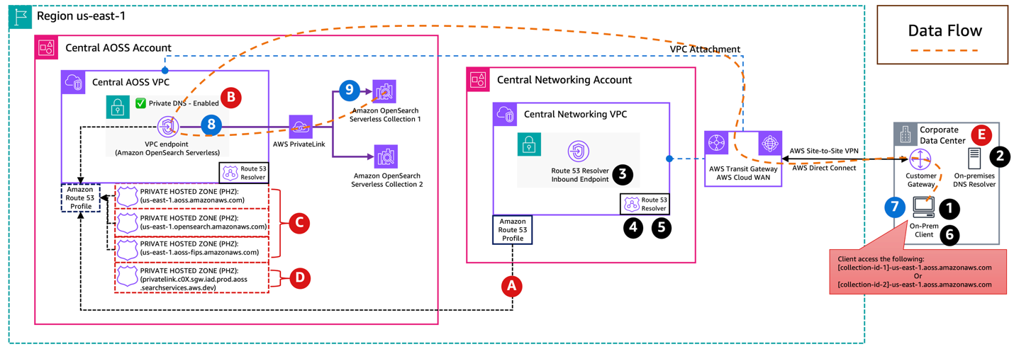
The following diagram illustrates the architecture across these three components. It shows how DNS queries from on-premises clients are resolved through the Route 53 Profile and Inbound Resolver, and how data traffic reaches the OpenSearch Serverless collections using AWS PrivateLink.
(A) The Route 53 Profiles are created in the central networking account and shared through AWS Resource Access Manager (AWS RAM) with the central OpenSearch Serverless account. The central OpenSearch Serverless account associates the PHZs and interface VPC endpoint association with the shared Route 53 Profiles because that’s needed for end-to-end private DNS resolution.
(B) The central AOSS VPC contains an interface VPC endpoint for OpenSearch Serverless with Private DNS enabled. There are four Private Hosted Zones (PHZs):
(C) The first three PHZs must be manually associated with the Route 53 Profile.
(D) The fourth is automatically associated when the VPC endpoint is associated with the profile.
(E) On the on-premises side, the DNS resolver is configured with conditional forwarding for us-east-1.aoss.amazonaws.com, directing queries to the Route 53 Resolver Inbound Endpoint in the central networking account.
DNS resolution flow
Your on-premises client initiates a request to collection-id-1.us-east-1.aoss.amazonaws.com.
The on-premises DNS resolver has a conditional forwarder for us-east-1.aoss.amazonaws.com and forwards the query over AWS Direct Connect or AWS Site-to-Site VPN to the Route 53 Resolver inbound endpoint IPs in the central networking VPC.
The inbound resolver receives the query and passes it to the Route 53 VPC Resolver.
The VPC Resolver checks the Route 53 Profiles associated with the central networking VPC. The Profiles provide access to the visible and hidden PHZs from the central OpenSearch Serverless VPC.
The VPC Resolver uses the visible PHZ to match the wildcard CNAME *.us-east-1.aoss.amazonaws.com to the interface VPC endpoint (VPCE) DNS name. It then uses the hidden PHZ to resolve the VPCE DNS name to the private elastic network interface (ENI) IP addresses of the interface VPC endpoint in the central OpenSearch Serverless VPC.
The private ENI IP addresses are returned through the inbound resolver endpoint to the on-premises DNS resolver and back to the on-premises client.
Data flow
The on-premises client sends an HTTPS request to the resolved private ENI IP address with the TLS Server Name Indication (SNI) header set to collection-id-1.us-east-1.aoss.amazonaws.com, over AWS Direct Connect or AWS Site-to-Site VPN through AWS Transit Gateway or AWS Cloud WAN.
Traffic reaches the interface VPC endpoint ENIs in the central OpenSearch Serverless VPC.
The interface VPC endpoint forwards the request to the OpenSearch Serverless service, which routes to Collection 1.
To access Collection 2, the client follows the same flow using collection-id-2.us-east-1.aoss.amazonaws.com. The wildcard DNS resolves to the same interface VPC endpoint, and the OpenSearch Serverless service routes to the correct collection based on the hostname.
Pattern 2: Accessing multiple OpenSearch Serverless collections from spoke accounts using a centralized VPC endpoint and Route 53 Profiles
While Pattern 1 addresses on-premises access, you might also need to provide access from compute resources and distributed applications across multiple AWS accounts. With this pattern, any compute resource running within spoke account VPCs can privately access multiple OpenSearch Serverless collections hosted in a central OpenSearch Serverless VPC through a single shared interface VPC endpoint.
In the following example, we use an Amazon Elastic Compute Cloud (Amazon EC2) instance as a compute resource to illustrate the pattern. However, the same approach applies to any compute resource within the spoke VPC.
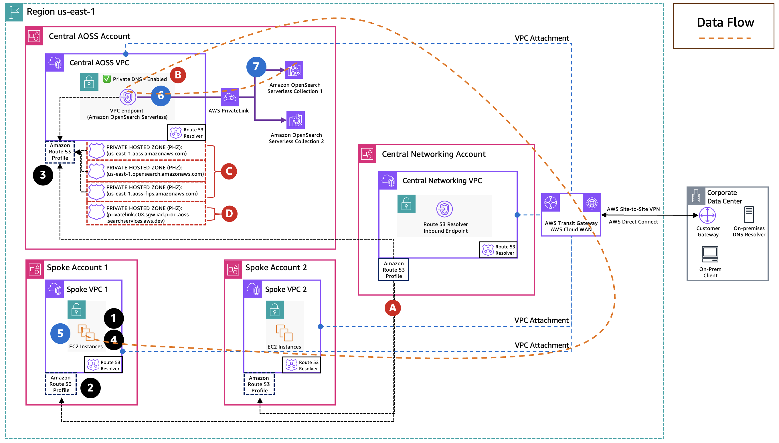
The following diagram illustrates this multi-account architecture, showing how spoke account VPCs resolve DNS and route data traffic to the central OpenSearch Serverless collections through the shared Route 53 Profile and AWS PrivateLink, alongside the on-premises access path from Pattern 1.
(A) The Route 53 Profiles, created in the central networking account, are shared via AWS RAM with both the OpenSearch Serverless account and the spoke accounts. The OpenSearch Serverless account associates its interface VPC endpoint and private hosted zones (PHZs) with the Profiles, while each spoke account associates the Profiles with its VPC. Spoke VPCs get full DNS resolution for OpenSearch Serverless collection endpoints without requiring their own interface VPC endpoints, PHZs, or manual DNS configuration.
(B) The central AOSS VPC contains an interface VPC endpoint for OpenSearch Serverless with Private DNS enabled. There are four Private Hosted Zones (PHZs):
(C) The first three PHZs must be manually associated with the Route 53 Profile.
(D) The fourth is automatically associated when the VPC endpoint is associated with the profile.
DNS resolution flow
An Amazon EC2 instance in Spoke VPC 1 initiates a request to collection-id-1.us-east-1.aoss.amazonaws.com and sends a DNS query to the Route 53 VPC Resolver.
The VPC Resolver finds the Route 53 Profiles associated with the spoke VPC, which carries the PHZs from the central OpenSearch Serverless account.
The visible PHZ matches the wildcard CNAME *.us-east-1.aoss.amazonaws.com to the VPCE DNS name. The hidden PHZ resolves the VPCE DNS name to the private ENI IP addresses of the interface VPC endpoint in the central OpenSearch Serverless VPC.
Route 53 returns the private ENI IP addresses to the Amazon EC2 instance.
Data flow
Your Amazon EC2 instance sends an HTTPS request to the resolved private ENI IP address with the TLS SNI header set to collection-id-1.us-east-1.aoss.amazonaws.com. This is routed through AWS Transit Gateway or AWS Cloud WAN to the central OpenSearch Serverless VPC.
The request arrives at the interface VPC endpoint ENIs in the central OpenSearch Serverless VPC.
The interface VPC endpoint forwards the request to the OpenSearch Serverless service, which routes to Collection 1.
To access Collection 2, the same flow applies using collection-id-2.us-east-1.aoss.amazonaws.com. The same applies to resources in Spoke Account 2 or other spoke accounts with the Route 53 Profiles associated.
AWS RAM Permission Configuration for Resource Association
When the central networking account shares the Route 53 Profiles through AWS RAM, the default AWS managed permissions policy (AWSRAMPermissionRoute53ProfileAllowAssociationActions) only grants actions for associating and disassociating the Profile with VPCs, viewing Profiles details, and listing associations. It does not include the route53profiles:AssociateResourceToProfile or route53profiles:DisassociateResourceFromProfile actions required for the OpenSearch Serverless account to associate its interface VPC endpoint and PHZs with the shared Profiles.
To enable this, the central networking account must create a custom managed permission in AWS RAM with the following actions:
route53profiles:AssociateProfile
route53profiles:AssociateResourceToProfile
route53profiles:DisassociateProfile
route53profiles:DisassociateResourceFromProfile
route53profiles:GetProfile
route53profiles:GetProfileResourceAssociation
route53profiles:ListProfileAssociations
route53profiles:ListProfileResourceAssociations
route53profiles:ListProfiles
This custom permission must be attached to the RAM resource share before the central OpenSearch Serverless account can associate its PHZs and interface VPC endpoint with the Profiles.
Cost considerations
The architecture patterns described in this post use several AWS services that may contribute to your overall costs, including Amazon Route 53 (hosted zones, DNS queries, and Resolver endpoints), and Route 53 Profiles. We recommend reviewing the official AWS pricing pages for the most current rates:
In this post, we showed how organizations can provide secure, private access to multiple OpenSearch Serverless collections from both on-premises environments and distributed AWS accounts using a single centralized interface VPC endpoint and Route 53 Profiles. This architecture centralizes OpenSearch Serverless collections and network infrastructure in a dedicated account, using Route 53 Profiles to propagate DNS across accounts. This eliminates per-account VPC endpoints, manual PHZ associations, and custom DNS configuration in spoke accounts.
This pattern is a good fit when a single team or business unit manages OpenSearch Serverless collections centrally. However, many enterprises have business units that need to independently manage their own OpenSearch Serverless collections in separate AWS accounts, each with their own interface VPC endpoints, security policies, and collection lifecycle. In Part 2, we explore how the architecture changes to support this distributed ownership model, where each business unit runs OpenSearch Serverless in their own account while still relying on centralized network connectivity and DNS management through Route 53 Profiles. We will cover how DNS resolution and the Route 53 Profiles configuration adapt when interface VPC endpoints and collections are spread across multiple accounts.
Last week was an incredible whirlwind: a round of meetups, hands-on workshops, and career discussions across Kenya that culminated with the AWS Student Community Day at Meru University of Science and Technology, with keynotes from my colleagues Veliswa and Tiffany, and sessions on everything from GitOps to cloud-native engineering, and a whole lot of AI agent building.
JAWS Days 2026 is the largest AWS Community Day in the world, with over 1,500 attendees on March 7th. This event started with a keynote speech on building an AI-driven development team by Jeff Barr, and included over 100 technical and community experience sessions, lightning talks, and workshops such as Game Days, Builders Card Challenges, and networking parties.
Now, let’s get into this week’s AWS news…
Last week’s launches Here are some launches and updates from this past week that caught my attention:
Introducing Amazon Connect Health, Agentic AI Built for Healthcare — Amazon Connect Health is now generally available with five purpose-built AI agents for healthcare: patient verification, appointment management, patient insights, ambient documentation, and medical coding. All features are HIPAA-eligible and deployable within existing clinical workflows in days.
Policy in Amazon Bedrock AgentCore is now generally available — You can now use centralized, fine-grained controls for agent-tool interactions that operate outside your agent code. Security and compliance teams can define tool access and input validation rules using natural language that automatically converts to Cedar, the AWS open-source policy language.
Introducing OpenClaw on Amazon Lightsail to run your autonomous private AI agents — You can deploy a private AI assistant on your own cloud infrastructure with built-in security controls, sandboxed agent sessions, one-click HTTPS, and device pairing authentication. Amazon Bedrock serves as the default model provider, and you can connect to Slack, Telegram, WhatsApp, and Discord.
AWS announces pricing for VPC Encryption Controls — Starting March 1, 2026, VPC Encryption Controls transitions from free preview to a paid feature. You can audit and enforce encryption-in-transit of all traffic flows within and across VPCs in a region, with monitor mode to detect unencrypted traffic and enforce mode to prevent it.
AWS Elastic Beanstalk now offers AI-powered environment analysis — When your environment health is degraded, Elastic Beanstalk can now collect recent events, instance health, and logs and send them to Amazon Bedrock for analysis, providing step-by-step troubleshooting recommendations tailored to your environment’s current state.
AWS simplifies IAM role creation and setup in service workflows — You can now create and configure IAM roles directly within service workflows through a new in-console panel, without switching to the IAM console. The feature supports Amazon EC2, Lambda, EKS, ECS, Glue, CloudFormation, and more.
Accelerate Lambda durable functions development with new Kiro power — You can now build resilient, long-running multi-step applications and AI workflows faster with AI agent-assisted development in Kiro. The power dynamically loads guidance on replay models, step and wait operations, concurrent execution patterns, error handling, and deployment best practices.
Amazon GameLift Servers launches DDoS Protection — You can now protect session-based multiplayer games against DDoS attacks with a co-located relay network that authenticates client traffic using access tokens and enforces per-player traffic limits, at no additional cost to GameLift Servers customers.
For a full list of AWS announcements, be sure to keep an eye on the What’s New with AWS page.
From AWS community Here are my personal favorite posts from AWS community and my colleagues:
When the Model Is the Machine — Mike Chambers built an experimental app where an AI agent generates a complete, interactive web application at runtime from a single prompt — no codebase, no framework, no persistent state. A thought-provoking exploration of what happens when the model becomes the runtime.
Upcoming AWS events Check your calendar and sign up for upcoming AWS events:
AWS Community GameDay Europe — Think you know AWS? Prove it at the AWS Community GameDay Europe on March 17, a gamified learning event where teams compete to solve real-world technical challenges using AWS services.
AWS at NVIDIA GTC 2026 — Join us at our AWS sessions, booths, demos, and ancillary events in NVIDIA GTC 2026 on March 16 – 19, 2026 in San Jose. You can receive 20% off event passes through AWS and request a 1:1 meeting at GTC.
AWS Summits — Join AWS Summits in 2026: free in-person events where you can explore emerging cloud and AI technologies, learn best practices, and network with industry peers and experts. Upcoming Summits include Paris (April 1), London (April 22), and Bengaluru (April 23–24).
AWS Community Days — Community-led conferences where content is planned, sourced, and delivered by community leaders. Upcoming events include Slovakia (March 11), Pune (March 21), and the AWSome Women Summit LATAM in Mexico City (March 28)
This is a guest post by Jeffrey Wang, Co-Founder and Chief Architect at Amplitude in partnership with AWS.
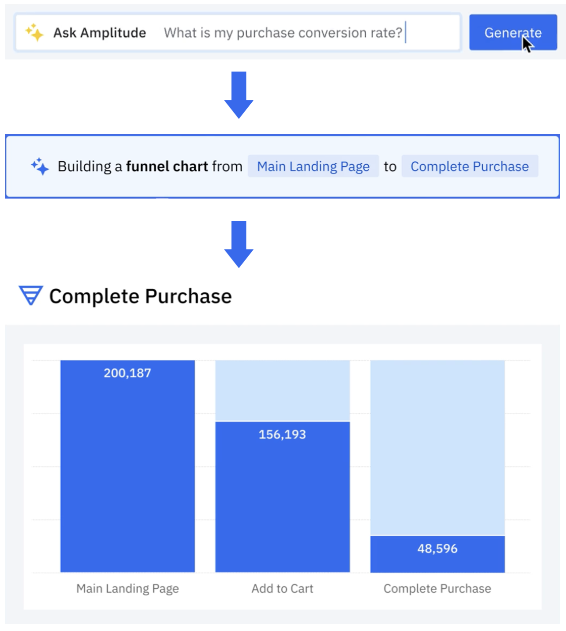
Amplitude is a product and customer journey analytics platform. Our customers wanted to ask deep questions about their product usage. Ask Amplitude is an AI assistant that uses large language models (LLMs). It combines schema search and content search to provide a customized, accurate, low latency, natural language-based visualization experience to end customers. Ask Amplitude has knowledge of a user’s product, taxonomy, and language to frame an analysis. It uses a series of LLM prompts to convert the user’s question into a JSON definition that can be passed to a custom query engine. The query engine then renders a chart with the answer, as illustrated in the following figure.
Amplitude’s search architecture evolved to scale, simplify, and cost-optimize for our customers, by implementing semantic search and Retrieval Augmented Generation (RAG) powered by Amazon OpenSearch Service. In this post, we walk you through Amplitude’s iterative architectural journey and explore how we address several critical challenges in building a scalable semantic search and analytics platform.
Our primary focus was on enabling semantic search capabilities and natural language chart generation at scale, while implementing a cost-effective multi-tenant system with granular access controls. A key objective was optimizing the end-to-end search latency to deliver rapid results. We also tackled the challenge of empowering end customers to securely search and use their existing charts and content for more sophisticated analytical inquiries. Additionally, we developed solutions to handle real-time data synchronization at scale, making sure constant updates to incoming data could be processed while maintaining consistently low search latency across the entire system.
RAG and vector search with Ask Amplitude
Let’s take a brief look at why Ask Amplitude uses RAG. Amplitude collects omnichannel customer data. Our end customers send data on user actions that are performed in their platforms. These actions are recorded as user-generated events. For example, in the case of retail and ecommerce customers, the types of user events include “product search,” “add to cart,” “checked out,” “shipping option,” “purchase,” and more. These events help define the customer’s database schema, outlining the tables, columns, and relationships between them. Let’s consider a user question such as “How many people used 2-day shipping?” The LLM needs to determine which elements of the captured user events are pertinent to formulating an accurate response to the query. When users ask a question to Ask Amplitude, the first step is to filter the relevant events from OpenSearch Service. Rather than feeding all event data to the LLM, we take a more selective approach for both cost and accuracy reasons. Because LLM usage is billed based on token count, sending complete event data would be unnecessarily expensive. More importantly, providing too much context can degrade the LLM’s performance—when faced with thousands of schema elements, the model struggles to reliably identify and focus on the relevant information. This information overload can distract the LLM from the core question, potentially leading to hallucinations or inaccurate responses. This is why RAG is the preferred approach. To retrieve the most relevant items from the product usage schema, a vector search is performed. This is effective even in situations when the question might not refer to the exact words that are in the customer’s schema. The following sections walk through the iterations of Amplitude’s search journey.
Initial solution: No semantic search
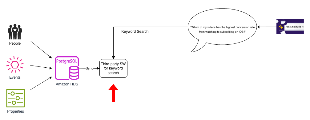
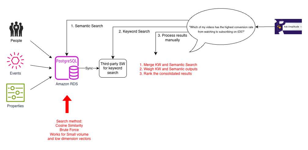
We used Amazon Relational Database Service (Amazon RDS) for PostgreSQL as the primary database to store our people, events, and properties data. However, as the following diagram shows, we had a separate, third-party store to implement keyword search. We had to bring in data from PostgreSQL to this third-party search index and keep it updated.
This architecture was simple but had two key shortcomings: there were no natural language capabilities in our search index, and the search index supported only keyword search.
Iteration 1: Brute force cosine similarity
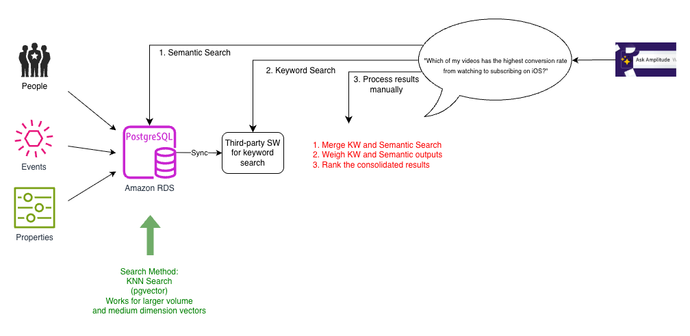
To improve our search capability, we considered several prototypes. Because data volumes for most customers were not very large, it was quick to build a vector search prototype using PostgreSQL. We transformed user interaction data into vector embeddings and used array cosine similarity to compute similarity metrics across the dataset. This alleviated the need for custom similarity computation. The vector embeddings captured nuanced user behavior patterns using PostgreSQL capabilities without additional infrastructure overhead. This is generally called the brute force method, where an incoming query is matched against all embeddings to find its top (K) neighbors by a distance measure (cosine similarity in this case). The following diagram illustrates this architecture.
Enabling semantic search was a big improvement over traditional search for users who might use different terms to refer to the same concepts, such as “hours of video streamed” or “total watch time”. However, although this worked for small datasets, it was slow because the brute force method had to compute cosine similarity for all pairs of vectors. This was amplified as the number of elements in the events schema, the complexity of questions, and expectations of quality grew. Additionally, Ask Amplitude answers needed to blend both semantic and keyword search. To support this, each search query had to be implemented as a three-step process involving multiple calls to separate databases:
Retrieve the semantic search results from PostgreSQL.
Retrieve the keyword search results from our search index.
In the application, semantic search results and keyword search results were combined using pre-assigned weights, and this output was dispatched to the Ask Amplitude UI.
This multi-step manual approach made the search process more complex.
Iteration 2: ANN search with pgvector
As Amplitude’s customer base grew, Ask Amplitude needed to scale to accommodate more customers and larger schemas. The goal was not just to answer the question at hand, but to teach the user how to build an end-to-end analysis by guiding them iteratively. To this end, the embeddings needed to store and index contextually rich semantic content. The team experimented with bigger, higher dimensionality embeddings and had anecdotal observations of vector dimensionality appearing to impact the effectiveness of the retrieval. Another requirement was to support multilingual embeddings.
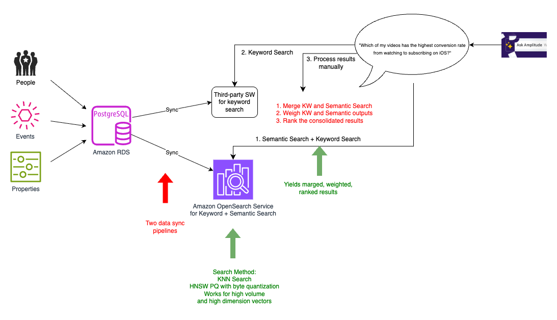
To support a more scalable k-NN search, the team switched to pgvector, a PostgreSQL extension that provides powerful functionalities for with vectors in high-dimensional space. The following diagram illustrates this architecture.
Pgvector was able to support k-nearest neighbor (k-NN) similarity search for larger dimensionality vectors. As the number of vectors grew, we switched to indexes that allowed approximate nearest neighbor (ANN) search, such as HNSW and IVFFlat.
For customers with larger schemas, calculating brute force cosine similarity was slow and expensive. We found a performance difference when we moved to ANN enabled by pgvector. However, we still needed to deal with the complexity introduced by the three-step process of querying PostgreSQL for semantic search, a separate search index for keyword search, and then stitching it all together.
Iteration 3: Dual sync to keyword and semantic search with OpenSearch Service
As the number of customers grew, so did the number of schemas. There were hundreds of millions of schema entries in the database, so we sought a performant, scalable, and cost-effective solution for k-NN search. We explored OpenSearch Service and Pinecone. We chose OpenSearch Service because we could combine keyword and vector search capabilities. This was convenient for four reasons:
Simpler architecture – Positioning semantic search as a capability in an existing search solution, as we observed in OpenSearch Service, makes for a simpler architecture than treating it as a separate specialized service.
Lower-latency search – The ability to effectively organize and catalog search data was fundamental to how we generated answers. Augmenting semantic search to our existing pipeline by combining both into one query provided lower latency querying.
Reduced need for data synchronization – Keeping the database in sync with the search index was critical to the accuracy and quality of answers. With the alternatives that we looked at, we would have to maintain two synchronization pipelines, one for keyword search index and the other for a semantic search index, complicating the architecture and increasing the chances of experiencing out-of-sync results between keyword and semantic search results. Synchronizing them into one place was easier than synchronizing them into multiple places and then combining the signals at query time. With a combined keyword and vector search capabilities of OpenSearch Service, we now needed to synchronize only one primary database on PostgreSQL with the search index.
Minimized performance impact to source data updates – We found that synchronizing data to another search index is a complex problem because our dataset changes constantly. With every new customer, we had hundreds of updates every second. We had to make sure the latency of these updates wasn’t impacted by the sync process. Collocating search data with vector embeddings obviated the need for multiple sync processes. This helped us avoid additional latency in the primary database, due to the sync processes encroaching upon database update traffic.
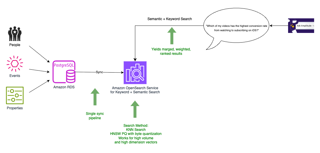
Although our previous third-party search engine specialized in fast ecommerce search, this wasn’t aligned with Amplitude’s specific needs. By migrating to OpenSearch Service, we simplified our architecture by reducing two synchronization processes to one. We phased out the current search platform gradually. This meant we temporarily continued to have two synchronization processes, one with current platform and another to the combined keyword and semantic search index on OpenSearch Service, as shown in the following diagram.
In addition to the pros of k-NN search identified in the previous iteration, moving to OpenSearch Service helped us realize three key benefits:
Reduced latency – Instead of collocating the embeddings with primary data, we were able to collocate with our search index. The search index is where our application needed to run our queries to pick out user events that are relevant to the question being asked and send this as context sent to the LLM. Because the search text, metadata, and embeddings were all in one place, we needed only one hop for all our search requirements, thereby improving latency.
Reduced compute power – We had anywhere between 5,000–20,000 elements in the user events schema. We didn’t need to send the entire schema to the LLM, because each user query required only 20–50 relevant elements. With the efficient filtering capabilities of OpenSearch Service, we were able to narrow down the vector search space by using tenant-specific metadata, significantly reducing compute requirements across our multi-tenant environment.
Improved scalability – With OpenSearch Service, we could take advantage of additional capabilities such as HNSW product quantization (PQ) and byte quantization. Byte quantization made it possible to handle the scale of millions of vector entries with minimal reduction in recall, but with improvement to cost and latency.
However, in this interim solution, our data wasn’t fully migrated to OpenSearch Service yet. We still had the old pipeline along with the new pipeline, and had to perform dual syncing. This was only temporary, as we phased out the old search index, and the old pipeline served as a baseline to compare with in terms of performance and recall.
Iteration 4: Hybrid search with OpenSearch Service
In the final architecture, we were able to migrate all our data to OpenSearch Service, which also served as our vector database, as shown in the following diagram.
We now had to perform just one data synchronization from the PostgreSQL database to the combined search and vector index, allowing the resources on the database to focus on transactional traffic. OpenSearch Service provides merging, weighting, and ranking of the search results as part of the same query. This obviated the need to implement them as a separate module in our application, effectively resulting in a single, scalable hybrid search (combined keyword-based (lexical) search and vector-based (semantic) search). With OpenSearch Service, we could also experiment with the new integration with Amazon Personalize.
Evolving RAG to draw upon user-generated content
Our customers wanted to ask deeper questions about their product usage that couldn’t be answered just by looking at the schema (the structure and names of the data columns) alone. Simply knowing the column names in a database doesn’t necessarily reveal the meaning, values, or proper interpretation of that data. The schema alone provides an incomplete picture. A naïve approach would be to index and search all data values instead of searching just the schema. Amplitude avoids this for scalability reasons. The cardinality and volume of event data (potentially trillions of event records) makes indexing all values cost prohibitive. Amplitudes hosts about 20 million charts and dashboards across all Amplitude customers. This user-generated content is valuable. We observed that we can better understand the meaning and context by analyzing how other users have previously visualized data.For example, if a user asks about “2-day shipping,” Amplitude first checks if the data schema contains columns with relevant names like “shipping” or “shipping method”. If such columns exist, it then examines the potential values in those columns to find values related to 2-day shipping. Amplitude also searches user-created content (charts, dashboards, and more) to see if anyone else at the company has already visualized data related to 2-day shipping. If so, it can use that existing chart as a reference for how to properly filter and analyze the data to answer the question. To search this content efficiently, Amplitude employs a hybrid approach combining keyword and vector similarity (semantic) searches. For tenant isolation and pruning, we use metadata to filter by customer first, and then vector search.
Conclusion
In this post, we showed you how Amplitude built Ask Amplitude, an AI assistant using OpenSearch Service as a vector database to enable natural language queries of product analytics data. We evolved our system through four iterations, ultimately consolidating keyword and semantic search into OpenSearch Service, which simplified our architecture from multiple sync pipelines to one, reduced query latency by combining search operations, and enabled efficient multi-tenant vector search at scale using features like HNSW PQ and byte quantization. We extended the system beyond schema search to index 20 million user-generated charts and dashboards, using hybrid search to provide richer context for answering customer questions about product usage.
As natural language interfaces become increasingly prevalent, Amplitude’s iterative journey demonstrates the potential for harnessing LLMs and RAG using vector databases such as OpenSearch Service to unlock rich conversational customer experiences. By gradually transitioning to a unified search solution that combines keyword and semantic vector search capabilities, Amplitude overcame scalability and performance challenges while reducing architecture complexity. The final architecture using OpenSearch Service enabled efficient multi-tenancy and fine-grained access control and also facilitated low-latency hybrid search. Amplitude is able to deliver more natural and intuitive analytics capabilities to its customers by generating deeper insights and contextualizing data.
To learn more about how Ask Amplitude helps you express Amplitude-related concepts and questions in natural language, refer to Ask Amplitude. To get started with OpenSearch Service as a vector database, refer to Amazon OpenSearch Service as a Vector Database.
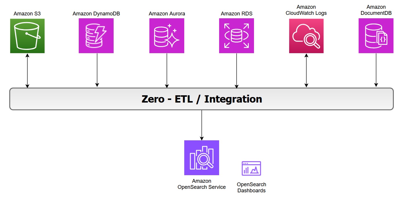
Amazon OpenSearch Service is a fully managed service that reduces operational overhead, provides enterprise-grade security, high availability, and scalability, and enables you to quickly deploy real-time search, analytics, and generative AI applications. OpenSearch itself is an open-source, distributed search and analytics suite that supports a wide range of use cases, including real-time monitoring, log analytics, and full-text search. OpenSearch Service offers zero-ETL integrations with other Amazon Web Service (AWS) services, enabling seamless data access and analysis without the need for maintaining complex data pipelines.
Zero-ETL refers to a set of integrations designed to minimize or eliminate the need to build traditional extract, transform, load (ETL) pipelines. Traditional ETL processes can be time-consuming and difficult to develop, maintain, and scale. In contrast, zero-ETL integrations allow direct, point-to-point data movement and can also support querying across data silos without physically moving the data.
In this post, we explore various zero-ETL integrations available with OpenSearch Service that can help you accelerate innovation and improve operational efficiency. We cover following types of integrations, their key features, architecture, benefits, pricing, limitation and some general best practices.
The following diagram illustrates the zero-ETL integration architecture in AWS, showing how various AWS services feed data into OpenSearch Service and its associated dashboards:
Zero-ETL integration with Amazon S3
Amazon OpenSearch Service direct queries with Amazon S3 provides a zero-ETL integration to reduce the operational complexity of duplicating data or managing multiple analytics tools by enabling you to directly query their operational data, reducing costs and time to action.
Key features of this integration include:
In-place querying: You can use rich analytics capabilities of OpenSearch Service SQL and PPL directly on infrequently-queried data stored outside of OpenSearch Service in Amazon S3.
Selective data ingestion: You can choose which data to bring into OpenSearch Service for detailed analysis, optimizing costs and speeding up queries with indexes like skipping or covering indexes.
In log analytics use cases, we categorize operational log data into two types:
Primary data includes the most recent and frequently accessed logs used for real-time monitoring and analysis.
Secondary data consists of historical logs that are accessed less frequently but retained for compliance or trend analysis.
You can offload infrequently queried data, such as archival or compliance data, to Amazon S3. With direct query, you can analyze analytics from Amazon S3 without data movement or duplication. However, query performance in OpenSearch Service might slow down when you’re accessing external data sources due to factors like network latency, data transformation, or large data volumes. You can optimize your query performance by using OpenSearch indexes, such as a skipping index, covering index, or materialized view.
While Amazon S3 direct query integration with OpenSearch Service provides on-demand access to data stored in Amazon S3, it is important to remember that OpenSearch’s alerting, monitoring, anomaly detection, and security analytics capabilities can only operate on data that has been explicitly ingested into OpenSearch Service indices. These capabilities would not work with direct query with Amazon S3. However, it will work if the data is indexed with covering or materialized index.
Benefits
With direct queries with Amazon S3, you no longer need to build complex ETL pipelines or incur the expense of duplicating data in both OpenSearch Service and Amazon S3 storage. You also save time and effort by not having to move back and forth between different tools during your analysis.
Pricing
OpenSearch Service separately charges for the compute needed to query your external data in addition to maintaining indexes in OpenSearch Service. Costs for Direct Query is based on the data volume scanned, query execution time, query frequency and frequency with which the indexed data in OpenSearch is kept updated. For more information, see Amazon OpenSearch Service Pricing.
Considerations
In case you are using OpenSearch service to query directly data on Amazon S3, consider the limitations with Direct Query.
Use the COALESCE SQL function to handle missing columns and ensure results are returned.
Use limits on your queries to ensure you aren’t pulling too much data back.
If you plan to analyze the same dataset many times, create an indexed view to fully ingest and index the data into OpenSearch Service and drop it when you have completed the analysis.
Drop acceleration jobs and indexes when they’re no longer needed.
Ingest data into Amazon S3 using partition formats of year, month, day, hour to speed up queries.
When you build skipping indexes, use Bloom filters for fields with high cardinality and min/max indexes for fields with large value ranges. Bloom filters are a space efficient probabilistic data structure that lets you quickly check whether an item is possibly in a set. For high-cardinality fields, consider using a value-based approach to improve query efficiency.
Use Index State Management to maintain storage for materialized views and covering indexes.
Zero-ETL integration with Amazon CloudWatch Logs
Amazon CloudWatch Logs serves as a centralized monitoring and storage solution for log files generated across various AWS services. This unified logging service offers a highly scalable platform where all your logging data converges into one manageable system. It provides comprehensive functionality for log management, including real-time viewing, pattern searching, field-based filtering, and secure archival capabilities. By presenting all logs chronologically in a unified stream, CloudWatch Logs eliminates the complexity of managing multiple log sources, transforming diverse logging data into a coherent, time-ordered sequence of events.
The zero-ETL integration between Amazon CloudWatch and Amazon OpenSearch Service enables direct log analysis and visualization while avoiding data redundancy, thereby reducing both technical complexity and costs. You can now leverage two additional query languages alongside the existing CloudWatch Logs Insights QL when using CloudWatch Logs, while as an OpenSearch user, you gain the ability to query CloudWatch logs directly.
The enhanced CloudWatch Logs Insights console now incorporates OpenSearch PPL and SQL functionality. Users can perform complex log analysis using SQL JOIN operations and various functions (including JSON, mathematical, datetime, and string operations). The PPL option provides additional data filtering and analysis capabilities.
The integration offers ready-to-use dashboards for various AWS services like Amazon Virtual Private Cloud (VPC), AWS CloudTrail, and AWS Web Application Firewall (WAF). These pre-configured visualizations enable quick insights into metrics such as flow patterns, top users, data transfer volumes, and temporal analysis, without requiring manual dashboard configuration.
You can now analyze CloudWatch logs through OpenSearch UI Discover and execute SQL and PPL queries. At the writing of this post, the query execution is limited to 50 log groups.
The direct access and analysis of CloudWatch data within OpenSearch Service removes the need for traditional ETL processes, eliminates separate data ingestion pipelines and avoids data duplication. This streamlined approach significantly reduces both storage expenses and operational complexity. It delivers a more efficient data management solution that simplifies the entire workflow while maintaining cost-effectiveness.
Pricing
When you use OpenSearch Service direct queries, you incur separate charges for OpenSearch Service and the resource used to process and store your data on Amazon CloudWatch Logs. As you run direct queries, you see charges for OpenSearch Compute Units (OCUs) per hour, listed as DirectQuery OCU usage type on your bill.
For interactive queries, OpenSearch Service handles each query with a separate pre-warmed job, without maintaining an extended session.
For indexed view queries, the indexed data is stored in an OpenSearch Serverless collection where you are charged for data indexed (IndexingOCU), data searched (SearchOCU), and data stored in GB.
In addition to the OpenSearch Service “direct queries” general limitations, if you are direct querying data in CloudWatch Logs, the following limitations apply:
The direct query integration with CloudWatch Logs is only available on OpenSearch Service collections and the OpenSearch user interface.
OpenSearch Serverless collections have networked payload limitations of 100 MiB.
CloudWatch Logs supports VPC Flow Logs, CloudTrail, and AWS WAF dashboard integrations installed from the console.
Best practices
Besides the general recommendations of OpenSearch Service direct querying, when using OpenSearch Service to direct query data in CloudWatch Logs, the following is recommended:
Specify the log group names within logGroupIdentifier in logGroups command to query multiple log groups in one query, see Multi-log group functions.
Enclose certain fields in backticks to successfully query them when using SQL or PPL commands. Backticks are needed for fields with special characters, such as `@SessionToken` or `LogGroup-A` (non-alphabetic and non-numeric). Refer to CloudWatch Logs Recommendations to see an example.
Zero-ETL integration with Amazon DynamoDB
Amazon DynamoDB zero-ETL integration with OpenSearch Service lets you perform a search on your DynamoDB data by automatically replicating and transforming it without custom code or infrastructure. This zero-ETL integration uses Amazon OpenSearch Ingestion to synchronize data between Amazon DynamoDB and OpenSearch Service cluster or OpenSearch Serverless collection within seconds of it being available.
It uses DynamoDB export to Amazon S3 to create an initial snapshot to load into OpenSearch Service. After the snapshot has been loaded, the plugin uses DynamoDB Streams to replicate any further changes in near real time. Turn on point-in-time recovery (PITR) for export and the DynamoDB Streams feature for ongoing replication.
This feature allows you to capture item-level changes in your table and push the changes to a stream. Every item in tables is processed as an event in OpenSearch Ingestion and can be modified with processors. You can also specify index mapping templates within ingestion pipelines to ensure that your Amazon DynamoDB fields are mapped to the correct fields in your OpenSearch indices.
When configuring zero-ETL between DynamoDB and OpenSearch Service, consider the differences between the data models. You have the following options with data layout:
Passthrough: Each item in DynamoDB table is directly mapped to one document in OpenSearch Index.
Routing: A single DynamoDB table mapped to multiple OpenSearch Service indices. In DynamoDB, it is common to store denormalized data in one table to optimize for access patterns. For example, a single DynamoDB table containing both customer profiles and order information can be routed to separate OpenSearch Service indices:
Merge: In some use cases, you need to combine data from multiple DynamoDB tables into a single OpenSearch index. You can use AWS Lambda integration with OpenSearch Ingestion to perform lookups on other DynamoDB tables and merge data from multiple DynamoDB tables.
Pricing
There is no additional cost to use this feature apart from the cost of the existing underlying components, including OpenSearch Ingestion charges OpenSearch Compute Units (OCUs) which is used to replicate data between Amazon DynamoDB and OpenSearch Service. Furthermore, this feature uses Amazon DynamoDB Streams for the change data capture (CDC), and you incur the standard costs for Amazon DynamoDB Streams.
Considerations
Consider the following limitations when you set up an OpenSearch Ingestion pipeline for DynamoDB:
At the writing of this post, the OpenSearch Ingestion integration with DynamoDB doesn’t support cross-Region and cross-account ingestion.
An OpenSearch Ingestion pipeline supports only one DynamoDB table as its source.
Amazon RDS and Amazon Aurora integration with OpenSearch Service eliminates complex data pipelines and enables near real-time data synchronization between Amazon Aurora and Amazon RDS databases (including RDS for MySQL and RDS for PostgreSQL) with advanced search capabilities on transactional databases. You can use an OpenSearch Ingestion pipeline with Amazon RDS or Amazon Aurora to export existing data and stream changes (such as create, update, and delete) to OpenSearch Service domains and collections. The OpenSearch Ingestion pipeline incorporates change data capture (CDC) infrastructure to provide a high-scale, low-latency way to continuously stream data from Amazon RDS or Amazon Aurora.
This automated process keeps your data consistently up to date in OpenSearch Service, making it readily available for search and analysis purpose. The pipeline ensures data consistency by continuously polling or receiving changes from the Amazon Aurora cluster or Amazon RDS and updating the corresponding documents in the OpenSearch index. OpenSearch Ingestion supports end-to-end acknowledgement to ensure data durability. An OpenSearch Ingestion pipeline also maps incoming event actions into corresponding bulk indexing actions to help ingest documents. This keeps data consistent, so that every data change in Amazon RDS is reconciled with the corresponding document changes in OpenSearch.
There is no additional charge for using this feature beyond the cost of your existing underlying resources, such as OpenSearch Service, OpenSearch Ingestion pipelines (OCUs), and Amazon RDS or Amazon Aurora. Additional costs may include storage used for enabling enhanced binlogs for MySQL and WAL logs for PostgreSQL for change data capture. You also incur storage costs for snapshot exports from your database to Amazon S3 used for the initial data.
Considerations
Consider the following limitations when you set up the integration for Amazon RDS or Amazon Aurora:
Requires same-Region and same-account deployment, primary keys for optimal synchronization, and currently has no data definition language (DDL) statement support.
The integration only supports one Aurora PostgreSQL database per pipeline.
The existing pipeline configuration can’t be updated to ingest data from a different database and/or a different table. To update the database and/or table name of a pipeline, stop the pipeline and restart it with an updated configuration or create a new pipeline.
Ensure that the Amazon Aurora or Amazon RDS cluster has authentication enabled using AWS Secrets Manager, which is the only supported authentication mechanism.
Best practices
The following are some best practices to follow while setting up the integration with OpenSearch Service:
If a mapping template is not specified in OpenSearch, it automatically assigns field types using dynamic mapping based on the first document received. However, it is always recommended to define field types explicitly by creating a mapping template that suits your requirements.
To maintain data consistency, the primary and foreign keys of tables remain unchanged.
You can configure the dead-letter queues (DLQ) in your OpenSearch Ingestion pipeline. If you’ve configured the queue, OpenSearch Service sends all failed documents that can’t be ingested due to dynamic mapping failures to the queue.
Amazon Document DB is a fully managed database service built for JSON data management at scale. It offers built-in text and vector search functionalities. By leveraging OpenSearch Service, you can execute search analytics, including features like fuzzy matching, synonym detection, cross-collection queries, and multilingual search capabilities on DocumentDB data.
The zero-ETL integration initiates the process with a full historical data extraction to OpenSearch using an ingestion pipeline. After the initial data load is completed, the pipelines read from Amazon DocumentDB change streams ensuring near real-time data consistency between the two systems. OpenSearch organizes the incoming data into indexes, with flexibility to either consolidate data from a DocumentDB collection into a single index or partition data across multiple indices. The ingestion pipelines synchronize all create, update, and delete operations from the DocumentDB collection, maintaining corresponding document modifications in OpenSearch. This ensures both data systems remain synchronised.
The pipelines offer configurable routing options, allowing data from a single collection to be written to one index or conditionally route to multiple indexes. Users can configure ingestion pipelines to stream data from Amazon DocumentDB to OpenSearch Service through three primary modes namely full load only, streaming change events without initial full load and full load followed by change streams. You can also monitor the state of ingestion pipelines in the OpenSearch service console. Additionally, you can use Amazon Cloudwatch to provide real-time metrics and logs and setting up alerts.
Pricing
There is no additional charge for using this feature apart from the cost of your existing underlying resources, including OpenSearch Service, OpenSearch Ingestion pipelines (OCUs), and Amazon DocumentDB. The integration performs an initial full load of Amazon DocumentDB data and continuously streams ongoing changes to OpenSearch Service using change streams. The change streams feature is disabled by default and does not incur any additional charges until the feature is enabled. Using change streams on a DocumentDB cluster incurs additional read and write input/output (I/O), as well as storage costs.
AWS Secrets Manager is the only supported authentication mechanism.
You can’t update an existing pipeline configuration to ingest data from a different database and/or a different collection. To update the database and/or collection name of a pipeline, create a new pipeline.
Best practices
The following are some best practices to follow while setting up the DocumentDB zero-ETL with OpenSearch Service:
Configure dead-letter queues (DLQ) to handle any failed document ingestion.
Configure AWS Secrets Manager and enable secrets rotation to provide the pipeline secure access.
If you’re using change streams in DocumentDB, it’s important to extend the retention period to up to 7 days. This ensures you don’t lose any data changes during the ingestion process.
With zero-ETL integrations, you can use the powerful search and analytics features of OpenSearch Service directly on your latest database data. These include full-text search, fuzzy search, auto-complete, and vector search for machine learning (ML) workloads—enabling intelligent, real-time experiences that enhance your applications and improve user satisfaction. This integration uses change streams to automate the synchronisation of transactional data from Amazon Aurora, Amazon RDS, Amazon DynamoDB and Amazon DocumentDB to OpenSearch Service without manual intervention. Once the data is available in OpenSearch Service, you can perform real-time searches to quickly retrieve relevant results for your applications.This eliminates the need for manual Extract-Transform-Load (ETL) processes, reduces operational complexity, and accelerates time-to-insight for real-time dashboards, search, and analytics.
Conclusion
In this post, you learned that zero-ETL integrations represent a significant advancement in simplifying data analytics workflows and reducing operational complexity. As you’ve explored throughout this post, these integrations offer several advantages such as elimination of complex ETL pipelines and reduced infrastructure and operational costs by removing the need for intermediate storage and processing that enhance developer productivity.
It is time to accelerate your analytics journey with OpenSearch Service zero ETL – where your data flows seamlessly, eliminating complex pipelines and delivering real-time insights. Get started with Amazon OpenSearch Service or learn more about integrations with other services and applications in the AWS documentation.
Today, we’re excited to announce the general availability of the collection groups feature for Amazon OpenSearch Serverless. With this feature you can reduce compute costs for multi-tenant workloads while creating secure tenant boundaries through per-tenant encryption, giving you the flexibility to balance cost efficiency with the exact level of isolation and security your applications requires.
Amazon OpenSearch Serverless is a serverless deployment option for Amazon OpenSearch Service, that eliminates the complexity of infrastructure management for running search and analytics workloads at scale. It automatically provisions and scales resources to deliver fast data ingestion rates and millisecond response times, even as usage patterns change. For organizations that are managing multi-tenant environments, data isolation, where the tenant’s data must be encrypted and protected (often with their own encryption keys), is a compliance requirement.
Previously, OpenSearch Serverless provided maximum security through physical isolation: each AWS Key Management Service key (KMS key) required dedicated OpenSearch Compute Units (OCUs) to maintain complete physical data separation. While this architecture provided the highest level of protection, it created challenges for multi-tenant deployments at scale. For customers managing multiple tenants with shared encryption keys, OCU resources are efficiently pooled, making the economics favorable. However, customers managing large numbers of smaller tenants, each requiring their own KMS key for data isolation, faced a challenge with higher cost. With dedicated OCU resources needed per unique key, the infrastructure costs could become prohibitive when individual tenants required only a fraction of an OCU’s capacity. This particularly impacted service providers wanting to offer bring your own key (BYOK) capabilities to their customers, forcing them to either absorb unsustainable costs or limit their service offerings.
OpenSearch Serverless has always provided flexible capacity management with maximum OCU settings to help you control costs. For most workloads, this model works seamlessly capacity scales up and down in response to demand, so you only pay for what you use. However, some workload patterns are simply better served by having a guaranteed baseline of compute ready to go from the start. Workloads with sudden traffic spikes, high-speed data ingestion pipelines, or load testing scenarios benefit from having capacity pre-allocated, so that the first requests are handled with the same responsiveness as any other. Similarly, multi-tenant architectures and time-sensitive operations often require predictable, consistent performance from the moment a collection becomes active.
Flexible controls with collection groups
Collection groups give you flexible control over security boundaries and resource allocation. Instead of forcing a one-size-fits-all approach, you can now tailor your architecture to match your specific security and cost requirements. Here’s how it works:
Define your security boundary that matches your need: Collection groups is a logical security construct for related collections. Each collection groups maintains strong isolation with physically separated memory, CPU and disk from other collection groups, ensuring robust security boundaries between different security constructs.
Share resources across encryption keys: Allocate collections to your collection groups regardless of whether they share KMS keys or use separate ones. Collections with different encryption keys can now share OCU resources within the same security boundary, dramatically reducing costs while maintaining full encryption protection and logical separation for each tenant.
Deploy with flexible network access: Collection groups support collections with different network access types, allowing you to combine collections with public endpoints and VPC endpoints within the same group. This flexibility lets you match your security and connectivity requirements while benefiting from shared resource management across all collections in the group.
Control cost and performance: Set maximum OCUs to cap spending and minimum OCUs to guarantee baseline performance. This dual control gives you a defined resource envelope for each collection groups, eliminating cost surprises while ensuring consistent performance.
Optimize with insights: Access detailed CloudWatch metrics showing resource consumption, relative usage patterns, and latency across collection groups. These insights help you right-size allocations, identify optimization opportunities, and tune performance based on actual workload behavior.
With collection groups, you now have full control over resource allocation through both minimum and maximum OCU settings
Maximum OCUs: Cost control
Set an upper limit on resources to prevent runaway scaling and control costs per collection groups. This helps ensure you never exceed your budget, even during unexpected traffic spikes. Collection groups capacity limits operate independently from account-level limits. Account-level maximum OCU settings apply only to collections not associated with any collection groups, while collection groups maximum OCU settings apply to collections within that specific group. The sum of (Max OCUs across all your collection groups + Max OCU setting at the account level) should be less than your Service Quota Max OCUs allowed for your account. This separation gives you granular cost control across different security contexts.
Minimum OCUs: Performance guarantees
Define the baseline compute resources that will always be allocated to your collection groups, for consistent performance and resource availability. These OCUs are reserved exclusively for your collection groups and provide:
Instant availability with no cold starts: Your collections benefit from instant availability without scaling delays. Resources are always warm and ready, eliminating scaling delays when traffic arrives.
Guaranteed capacity: Resources are always available, even during periods of low activity or when competing with other collection groups, ensuring predictable performance even during low-traffic periods.
Predictable costs: Minimum OCUs are charged continuously, providing you with reserved capacity in exchange for predictable billing giving you cost certainty in exchange for guaranteed performance. This reserved baseline serves as the foundation for auto-scaling, which expands capacity up to your maximum limit as demand increases.
This combination gives you the flexibility to balance cost optimization with performance guarantees based on your specific requirements.
Multi-tenant cost economics with collection groups
Managing costs in multi-tenant architectures has always required balancing isolation, performance, and efficiency often at the expense of one another. Collection groups change that equation by enabling shared capacity across collections without sacrificing security boundaries. The following details how this plays out when you work with collection groups or without.
Before collection groups: Consider a customer with 10 tenants, each requiring their own KMS key for data isolation. Most of these tenants have modest data requirements typically 10-100GB, with the majority on the smaller end of that range. Managing dedicated resources for each tenant’s encryption key, regardless of their actual capacity needs, created operational complexity and cost challenges at scale.
With collection groups: The same customer can now group their tenants with similar security requirements into the collection groups, sharing OCU resources across collections. Tenants requiring only a small portion of OCU capacity no longer force the allocation of dedicated resources, reducing costs by up to 90% for large number of smaller tenant workloads.
With minimum OCU configuration: Premium tenants can be placed in collection groups with minimum OCUs set to guarantee performance, while standard tenants use collection groups with lower minimum thresholds for cost efficiency.
The following table illustrates how these cost savings play out across different tenant configurations, comparing infrastructure costs with and without collection groups across varying data sizes and query loads.
Number of tenants with unique KMS keys
Data size and query parameters
Cost with complete data isolation (without collection groups)
Cost with collection groups
Additional comments
10
Data size: 60GB or less
Query: Not needing more than base OCU (1 for redundant collection) compute
$3,500
$350
10x Savings in cost.
10
Data size: 60GB or less
Query: More than base OCU (1 for redundant collection) compute during peak times (For example – 5 additional OCUs per tenant without collection groups & 40 OCUs across all tenants based with collection groups due to benefit of shared infra).
$3500 + Peak time scale out per tenant ($8650)
$350+ Peak time scale out ($6912).
The system will scale up when there is additional query load, additional OCUs are deployed during this time. However when the load scales back, the system will scale-in to base OCU’s.
10
Data size: Sample data size in GB per tenant [3, 5, 7, 8, 10, 15, 18, 25, 28, 150]
Query: Can handle queries upto certain level with minimum OCU for the data size and then scales out on load.
For the sample data sizes, minimum OCU requirement will be [2, 2, 2, 2, 2, 2, 2, 2, 2, 8] = 26 OCUs [$4492] + Peak time scale out per tenant
Minimum cost is determine by the number of OCUs required to hold the data across all tenants (120GB per OCU *2) + Peak time scale out.For the sample data sizes, 8 OCUs [$1382] + Peak time scale out per tenant
The system will scale up when there is additional query load, additional OCUs are deployed during this time. However when the load scales back, the system will scale-in to minimum number of OCU required to hold the data.
Note: Above calculations are made with assumption for redundant enabled collections. For non-redundant mode it will be half the above calculations.
Getting started with collection groups
Collection groups and minimum OCU configuration are available in all AWS Regions where OpenSearch Serverless is offered, at no additional charge. Collection groups offers a new organizational feature to create collection groups and add new collections directly to these groups for enhanced management capabilities. While your existing collections will continue to operate unchanged and remain independent of any collection groups, you can immediately start using collection groups for new collections to benefit from improved organization and workflow management.
Currently, only newly created collections can be associated with collection groups, and all collections within a group must be of the same type (search, time series, or vector search). Existing collections continue to operate independently with their current capacity management settings, and you cannot mix different collection types within a single collection groups. You can use the AWS Management Console, AWS CLI, AWS CloudFormation, or AWS CDK to create the collection groups. In the following section we will show you how you can create the collection groups using the OpenSearch Service console.
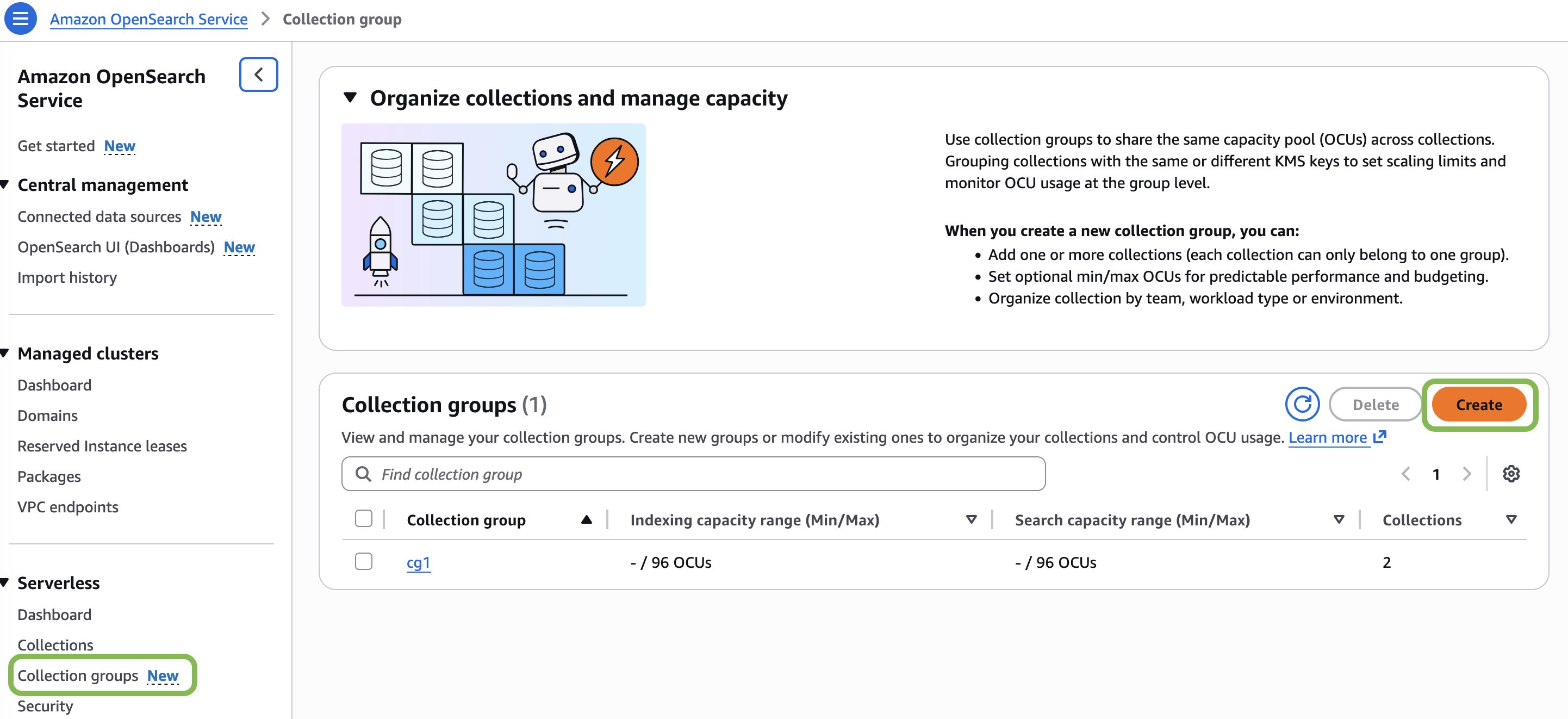
In the left navigation pane, choose Serverless, then choose Collection groups.
Choose Create collection groups.
For collection groups name, enter a name for your collection groups. The name must be 3-32 characters long, start with a lowercase letter, and contain only lowercase letters, numbers, and hyphens.
(Optional) For Description, enter a description for your collection groups.
In the Capacity management section, configure the OCU limits:
Maximum indexing capacity – The maximum number of indexing OCUs that collections in this group can scale up to.
Maximum search capacity – The maximum number of search OCUs that collections in this group can scale up to.
Minimum indexing capacity – The minimum number of indexing OCUs to maintain for consistent performance.
Minimum search capacity – The minimum number of search OCUs to maintain for consistent performance.
(Optional) In the Tags section, add tags to help organize and identify your collection groups.
In the left navigation pane, choose Serverless, then choose Collections.
Choose Create collection.
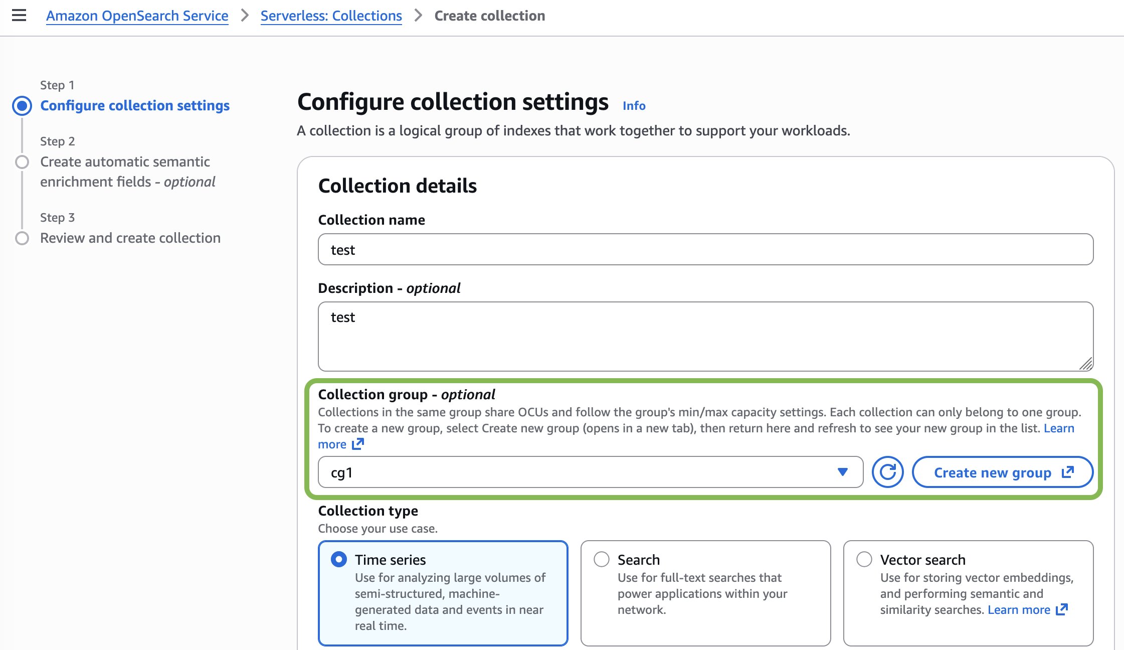
For Collection name, enter a name for your collection. The name must be 3-28 characters long, start with a lowercase letter, and contain only lowercase letters, numbers, and hyphens.
(Optional) For Description, enter a description for your collection.
In the Collection groups section, select the collection groups you want the collection to be assigned to. A collection can only belong to one collection groups at a time. (Optional) You can also choose to Create a new group. This will navigate you to the Create collection groups workflow. After you finish creating the collection groups, return to the step 1 of this procedure to begin creating your new collection.
Continue through the workflow to create the collection.
Managing collection groups
Once you’ve created your collection groups, you can update their settings as your architecture evolves. The Amazon OpenSearch Serverless documentation provides step-by-step guidance on how to edit and delete collection groups, including updating OCU limits and modifying group configurations using the AWS Management Console, CLI, and CloudFormation.
Conclusion
OpenSearch Serverless collection groups transform how you can architect multi-tenant deployments by offering flexible deployment modes that balance security requirements with operational efficiency. You can now choose the collection groups where you define logical security boundaries that allow collections, regardless of whether they share the same KMS key or use different KMS keys to share OCU resources.
This flexibility directly addresses the cost challenges that previously made multi-tenant deployments prohibitive. By consolidating collections within collection groups, you can reduce infrastructure costs while maintaining robust encryption and tenant isolation. Configuring both minimum and maximum OCUs for each collection groups solves the cold-start and capacity guarantee challenges: minimum OCUs ensure your collections maintain ready compute resources to handle high-speed ingestion, sudden traffic spikes, and load testing without performance degradation. Maximum OCUs provide cost predictability and spending controls. This dual configuration gives you a defined resource envelope that eliminates both the uncertainty of cold starts and the risk of runaway costs.
If you’ve ever shopped on Amazon, you’ve used Your Orders. This feature maintains your complete order history dating back to 1995, so you can track and manage every purchase you’ve made. The order history search feature lets you find your past purchases by entering keywords in the search bar. Beyond just finding items, it provides a straightforward way to repurchase the same or similar items, saving you time and effort.
Various features across Amazon’s shopping experience, such as Rufus and Alexa, use order history search to help you find your past purchases. Therefore, it’s important that order history search can locate your past purchased items as accurately and quickly as possible.
In this post, we show you how the Your Orders team improved order history search by introducing semantic search capabilities on top of our existing lexical search system, using Amazon OpenSearch Service and Amazon SageMaker.
Limitations of lexical search
Order history search uses lexical matching to find items from the entire order history of a customer that match at least one word of the search keywords. For example, if a customer searches for “orange juice,” the system retrieves all orange juice items as well as fresh oranges and other fruit juices the customer had previously ordered. Although lexical matching can provide a high recall of items with terms matching the search keywords precisely, it doesn’t work well for related or generic search keywords, like “health drinks” in this example.
Since the launch of Rufus, Amazon’s AI-enabled shopping assistant, a growing number of customers are experiencing a streamlined and richer shopping journey, including searching for their previous purchases with Rufus. Customers can now ask “Show me healthy drinks” without worrying about using lengthy, more precise terms like “kombucha”, “green tea”, and “protein shakes”. This makes the search experience more conversational and intent-based, presenting an opportunity to make item discovery more intuitive. For Rufus to answer order history searches with the same intuitive experience such as “Show me the healthy drinks I bought last year”, the underlying order history data store (“Your Orders”) needs semantic search capability to understand the underlying semantics of search keywords beyond the conventional lexical matching.
Challenges implementing semantic search
Implementing semantic search at our scale presented several technical challenges:
Scale – We needed to enable semantic search across billions of records corresponding to customers’ order history globally.
Zero downtime – We needed to keep the system 100% available while making changes on the backend to introduce semantic search.
Preventing search quality degradation – Semantic search is intended to improve the quality of search results. However, in some cases, it can reduce search quality. For example, if a customer remembers their item name exactly and wants to find only items matching that name, surfacing similar items in addition to the exactly matching items will increase crowding in results and make it harder to find the relevant item. Similarly, semantic search will not work for cases where the customer intends to search by identifier values, like order ID, which lack an inherent semantic meaning. For these scenarios, we use lexical search only.
Solution overview
Semantic search is powered by large language models (LLMs), which are mostly trained on human languages. These models can be adapted to take a piece of text in any language they were trained in and emit an embedding vector of a fixed length, irrespective of the input text length. By design, embedding vectors capture the semantic meaning of input text such that two semantically similar text strings have high cosine similarity computed on their respective embedding vectors. For semantic search on order history, the input text subject to embedding generation and similarity computation are the customer search phrases and the product text of purchased items.
We divide our solution into two parts:
Improving system scalability and resiliency for handling requests at scale – Before implementing semantic search, we needed to ensure our infrastructure could handle the increased computational load, leading us to adopt a cell-based architecture. This step is not needed for every use case, but systems with very high scale in terms of request or data volume can benefit a lot from its use before implementing a resource-intensive use case like semantic search.
Implementing semantic search – We began by evaluating the available embedding models, using the offline evaluation capabilities of Amazon Bedrock to test different models. After we selected our model, we could establish the infrastructure for generating embedding vectors.
Improving system scalability and resiliency
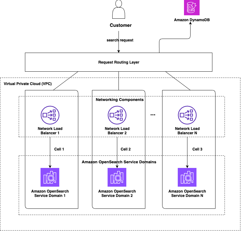
We used the cell-based architecture design pattern for improving our scalability and resiliency. A cell-based design entails partitioning the system into identical, smaller, self-contained chunks, or cells, which handle only a part of the overall traffic received by the system. The following diagram shows a high-level representation of a cell-based design for order history search.
Each cell serves a defined subset of our customers. Cells don’t need to communicate with one another to serve a customer request. Each customer is assigned to a cell and each request from that customer is routed to that cell. The OpenSearch Service domain in each cell holds data only for the subset customers that it is supposed to serve. The number of cells (N) and distribution of data among those cells depends on the business use case, but the goal is to achieve as even a distribution of data and traffic as possible.
The routing logic can be kept as simple or as sophisticated as the use case requires it to be. The cell assignment values can either be computed at runtime for each request, or they can be computed one time and written to a cache or persistent data store like Amazon DynamoDB, from where cell assignment values can be fetched for subsequent requests. For order history search, the logic was simple and quick enough to be executed at runtime for each request. Looking up cell assignment from a persistent data store is especially useful for cases where there is a risk of some cells becoming “heavier” than others over time. In such cases, it becomes easier to redistribute the heavy cell’s data by simply overriding cell assignment values for specific keys in the data store, instead of having to change the partitioning logic immediately, which might have an impact on data distribution across all the cells.
As the system’s load grows, the number of cells in the system can be increased to handle the additional traffic. Even without increasing the number of cells in the system, we can redistribute current data among the existing N cells by reassigning some keys from one or more heavily populated cells to different lightly populated cells to spread out the load more evenly across all the cells and make more efficient use of the infrastructure.
A cell-based architecture also helps make the system more resilient. For example, if we lose one cell, our capacity is diminished only by 1/N, instead of 100%. This arrangement can also be improved to reduce the capacity loss even further by assigning partitioning keys to two or more cells such that they get written to two or more cells. In such cases, loss of a single cell does not result in data loss.
Implementing semantic search
Implementing semantic search for our order history search required several key decisions and technical steps. We began by evaluating the available embedding models, using the offline evaluation capabilities of Amazon Bedrock to test different models against our specific business domain requirements. This evaluation process helped us identify which model would deliver the best performance for our use case. After we selected our model, we needed to establish the infrastructure for generating embedding vectors. We containerized our embedding model and registered it in Amazon Elastic Container Registry (Amazon ECR), then deployed it using SageMaker inference endpoints to handle the actual vector computation at scale.
For the search infrastructure itself, we chose OpenSearch Service to implement our semantic search capabilities. OpenSearch Service provided both the vector storage we needed and the search algorithms required to deliver relevant results to our users.
One of our biggest challenges was updating our historical data to support semantic search on existing orders. We built a data processing pipeline using AWS Step Functions to orchestrate the workflow and AWS Lambda functions to handle the actual vector generation for our legacy data, so we could provide semantic search for all the records we wanted to.
The following diagram illustrates the high-level architecture.
Model evaluation and selection
Order history search uses an embedding model trained on Amazon-specific data. Domain-specific training is critical because the generated embedding vectors must work well for the business context to return quality results.
We used an LLM-as-a-judge methodology with Anthropic’s Claude on Amazon Bedrock to evaluate candidate models. Anthropic’s Claude received prompts containing anonymized item text and search phrases from customer order history, then filtered and ranked items by relevance. These results served as ground truth for comparison.
We evaluated models using standard ranking metrics:
Normalized Discounted Cumulative Gain (NDCG) – Measures ranking quality against ideal order
Mean Reciprocal Rank (MRR) – Considers position of first relevant item
Precision – Rates accuracy of retrieved results
Recall – Rates ability to retrieve all relevant items
Search only through the requesting customer’s order history – We don’t want items from one customer’s order history showing up in search results for another customer
Search all of that customer’s history – We don’t want to miss showing an item that would have been relevant for the customer’s search phrase just because the search algorithm missed evaluating it for some reason
Our approach involves using OpenSearch Service to retrieve all items for the customer who issued the search query, calculating relevance scores for each of them against the search phrase, sorting by score, and returning top K results. This provides comprehensive results coverage for each customer.
Vector storage with OpenSearch Service
We used two OpenSearch Service features for efficient vector storage and search:
knn_vector datatype – Built-in support for storing embedding vectors. Existing domains can add this field type without reindexing, enabling exact kNN search across all records. We didn’t need approximate kNN because the number of records for most customers was small enough for exact kNN to scale.
Hybrid search refers to combining the results of lexical and semantic search to benefit from the strengths of each. The hybrid query capabilities of OpenSearch Service simplify implementing hybrid search by letting clients specify both types of queries in a single request. OpenSearch Service runs both queries in parallel, merges their results, normalizes the relevance scores of the sub-queries, and sorts results by the provided sort order (relevance score by default) before returning them to clients.
This gives clients the best of both types of searches. For example, there are certain scenarios where the search phrase doesn’t make much sense semantically, like when customers search by their orderId values. Semantic search is not designed for such cases; these are best served using keyword matching.
The hybrid search functionality helped save implementation effort and potential latency increase for order history search.
Updating historical data
After the infrastructure has been set up, newly ingested records are persisted with the relevant embedding vectors and support semantic search on those records. However, when customers search, they typically search for products they had purchased earlier. Therefore, the system might not help improve customer experience much unless the older records are updated to include the relevant embeddings. The approach to populate this data depends on the scale of the problem at hand.
Releasing the change to minimize potential customer impact
Our final step was to release the change to clients in a manner such that the impact of any potential problems is as small as possible. There are multiple ways to do that, including:
Implementing semantic search in a manner such that any transient issues in the semantic search flow make the logic fall back to lexical-only search, instead of failing the request completely. Even if semantic search doesn’t execute, the system should still be able to return results of lexical search to the client, instead of empty results.
Gating the change such that the default behavior remains lexical-only search and clients who need the semantic search feature must pass an additional flag in the request, for example, which executes the semantic or hybrid flow only for those requests.
Keeping the new flow behind a feature flag during the initial period such that it could be turned off completely if some critical problem is detected.
Examples of improved customer experience
The following are some examples of customer interactions with Rufus that required Rufus to query the respective customer’s order history to answer their question and give them the required pieces of information.
The following screenshots show how semantic search picks up wooden spoons for a “sustainable utensils” query and different kinds of chargers despite not having the keyword “charger” in the title description, in the case of the wall connector.
The following screenshots show how semantic search picks up relevant results even though the title description doesn’t include the queried keywords.
The semantic search feature of order history search helped Rufus fetch them and show to the customers. Before semantic search, Rufus wasn’t able to show any results to customers for such queries.
Business impact
Our solution resulted in the following key business impacts:
Customer experience improvements – The solution achieved 10% improvement in query recall, increasing the percentage of searches that return relevant results. It also reduced customer service contacts for issues related to locating past orders.
Partner integration success – The solution strengthened natural language processing capabilities for Alexa and Rufus, enhancing their ability to interpret order history queries. It also reduced the need for reranking and postprocessing by partner teams. We improved query success rate by 20%, meaning more customer searches now return at least one relevant item. We also observed enhanced result coverage by 48%, with semantic search consistently surfacing additional relevant matches that lexical search would have missed.
Conclusion
In this post, we showed you how we evolved Amazon order history search to support semantic search capabilities. This transition involved using cutting-edge AI technology while working within existing infrastructure limitations to develop solutions that avoided disruption and maintained SLAs during the feature upgrade. The implementation also involved backfilling, where billions of documents were processed at rates multiple times higher than normal ingestion to compute embedding vectors for previously purchased items. This operation required careful engineering and took advantage of the resilience OpenSearch Service offers even under extreme load.
Beyond the immediate implementation, this foundation enables continued innovation in search technology. The embedding vectors framework can incorporate improved models as they become available, and the architecture supports expansion into new capabilities such as personalization and multi-modal search.
You can get started with exact k-NN search today following the instructions in Exact k-NN search. If you’re looking for a managed solution for your OpenSearch cluster, check out Amazon OpenSearch Service.
Amazon OpenSearch Service is a fully managed service for search, analytics, and observability workloads, helping you index, search, and analyze large datasets with ease. Making sure your OpenSearch Service domain is right-sized—balancing performance, scalability, and cost—is critical to maximizing its value. An over-provisioned domain wastes resources, whereas an under-provisioned one risks performance bottlenecks like high latency or write rejections.
In this post, we guide you through the steps to determine if your OpenSearch Service domain is right-sized, using AWS tools and best practices to optimize your configuration for workloads like log analytics, search, vector search, or synthetic data testing.
Why right-sizing your OpenSearch Service domain matters
Right-sizing your OpenSearch Service domain provides optimal performance, reliability, and cost-efficiency. An undersized domain leads to high CPU utilization, memory pressure, and query latency, whereas an oversized domain drives unnecessary spend and resource waste. By continuously matching domain resources to workload characteristics such as ingestion rate, query complexity, and data growth, you can maintain predictable performance without overpaying for unused capacity.
Beyond cost and performance, right-sizing facilitates architectural agility. It helps make sure your cluster scales smoothly during traffic spikes, meets SLA targets, and sustains stability under changing workloads. Regularly tuning resources to match actual demand optimizes infrastructure efficiency and supports long-term operational resilience.
Key Amazon CloudWatch metrics
OpenSearch Service provides Amazon CloudWatchmetrics that offer insights into various aspects of your domain’s performance. These metrics fall into 16 different categories, including cluster metrics, EBS volume metrics, and instance metrics. To determine if your OpenSearch Service domain is misconfigured, monitor these common symptoms that indicate resizing or optimization may be necessary. These are caused by imbalances in resource allocation, workload demands, or configuration settings. The following table summarizes these parameters:
CloudWatch Metrics
Parameter
CPU Utilization Metrics
CPUUtilization: Average CPU usage across all data nodes.
Optimal range: 60-80% for sustained workloads
Primary control plane CPU utilization (for dedicated primary nodes): Average CPU usage on primary nodes.
Optimal range: Under normal conditions <50%
Memory Utilization Metrics
JVMMemoryPressure: Percentage of heap memory used across data nodes.
Optimal range: 65–85%
Note: With Garbage First Garbage Collector (G1GC), JVM may delay collections to optimize performance. Evaluate JVMMemoryPressure together with GC metrics (Old Gen usage and GC pause time) to confirm true pressure trends.
MasterJVMMemoryPressure: Heap usage on dedicated primary nodes.
Optimal range: <80%
Note: Occasional spikes are normal during state updates; sustained high memory pressure warrants scaling or tuning.
Storage Metrics
StorageUtilization: Percentage of storage space used.
Optimal range: 70–85%
FreeStorageSpace: Available storage in MB.
Critical threshold: When approaching the read-only threshold.
Node Level Search and Indexing Performance
(These latencies are not per-request latencies or rate, but at node level based on shards assigned to a node.)
SearchLatency: Average time for search requests.
Baseline establishment: Monitor during normal operations.
IndexingLatency: Average time for indexing operations.
Impact: Can indicate CPU or I/O bottlenecks.
SearchRate and IndexingRate: Requests per minute for search and indexing.
Usage: Correlate with latency metrics to understand performance impact.
Cluster Health Indicators
ClusterStatus.yellow and ClusterStatus.red:
Yellow status: Some replica shards are unassigned.
Red status: Some primary shards are unassigned (data loss risk).
Nodes
What it measures: Number of nodes in the cluster.
Usage: Track node failures and recovery patterns.
Signs of under-provisioning
Under-provisioned domains struggle to handle workload demands, leading to performance degradation and cluster instability. Look for sustained resource pressure and operational errors that signal the cluster is running beyond its limits. For monitoring, you can set CloudWatch alarms to catch early signals of stress and prevent outages or degraded performance. The following are critical warning signs:
High CPU utilization for data nodes (>80%) sustained over time (such as more than 10 minutes)
High CPU utilization for primary nodes (>60%) sustained over time (such as more than 10 minutes)
JVM memory pressure consistently high (>85%) for data and primary nodes
Storage utilization reaching high (>85%)
Increasing search latency with stable query patterns (increasing by 50% from baseline)
Frequent cluster status yellow/red events
Node failures under normal load conditions
When resources are constrained, the end-user experience suffers with slower searches, failed indexing, and system errors. The following are key performance impact indicators:
The following table summarizes CloudWatch metric symptoms, possible causes, and potential solutions.
CloudWatch metric symptom
Causes and solution
FreeStorageSpacedrops <20%
Storage pressure occurs when data volume outgrows local storage due to high ingestion, long retention without cleanup, or unbalanced shards. Lack of tiering (such as UltraWarm) further worsens capacity issues.
CPUUtilization and JVMMemoryPressure consistently >70%
High CPU or JVM pressure arises when instance sizes are too small or shard counts per node are excessive, leading to frequent GC pauses. Inefficient shard strategy, uneven distribution, and poorly optimized queries or mappings further spike memory usage under heavy workloads.
Solution: Address high CPU/JVM pressure by scaling vertically to larger instances (such as from r6g.large to r6g.xlarge) or adding nodes horizontally. Optimize shard counts relative to heap size, smooth out peak traffic, and use slow logs to pinpoint and tune resource-heavy queries.
SearchLatency or IndexingLatency spikes >500 milliseconds
Thread pool rejections often stem from resource contention like high CPU/JVM pressure or GC pauses. Inefficient shard sizing, over-sharding, and overly complex queries (deep aggregations, frequent cache evictions) further increase overhead and push tasks into rejection.
Solution: Reduce query latency by optimizing queries with profiling, tuning shard sizes (10–50 GB each), and avoiding over-sharding. Improve parallelism by scaling the cluster, adding replicas for read capacity, increasing cache through larger nodes, and setting appropriate query timeouts.
Thread pool rejections occur when high concurrent requests overflow queues beyond capacity, especially with undersized nodes limited by vCPU-based threads. Sudden unscaled traffic spikes further overwhelm pools, causing tasks to be dropped or delayed.
Solution: Mitigate thread pool rejections by enforcing shard balance across nodes, scaling horizontally to boost thread capacity, and managing client load with retries and reduced concurrency. Monitor search queues, right-size instances for vCPUs, and cautiously tune thread pool settings to handle bursty workloads.
ThroughputThrottle or IopsThrottle reach 1
I/O throttling arises when Amazon EBS or Amazon EC2 limits are exceeded, such as gp3’s 125 MBps baseline, or when burst credits are depleted due to sustained spikes. Mismatched volume types and heavy operations like bulk indexing without optimized storage further amplify throughput bottlenecks.
Solution: Address I/O throttling by upgrading to gp3 volumes with higher baseline or provisioning extra IOPS and consider I/O-optimized instances like i3/i4 families while monitoring burst balance. For sustained workloads, scale nodes or schedule heavy operations during off-peak hours to avoid hitting throughput caps.
Signs of over-provisioning
Over-provisioned clusters show consistently low utilization across CPU, memory, and storage, suggesting resources far exceed workload demands. Identifying these inefficiencies helps reduce unnecessary spend without impacting performance. You can use CloudWatch alarms to track cluster health and cost-efficiency metrics over 2–4 weeks to confirm sustained underutilization:
Low CPU utilization for data and primary nodes (<40%) sustained over time
Low JVM memory pressure for data and primary nodes (<50%)
Excessive free storage (>70% unused)
Underutilized instance types for workload patterns
Monitor cluster indexing and search latencies constantly as the cluster is being downsized—these latencies should not increase if the cluster is eliminating unused capacity. Also, it’s recommended to reduce nodes one at a time and continue to observe latencies to continue further downturn. By right-sizing instances, reducing node counts, and adopting cost-efficient storage options, you can align resources to actual usage. Optimizing shard allocation further supports balanced performance at a lower cost.
Best practices for right-sizing
In this section, we discuss best practices for right-sizing.
Iterate and optimize
Right-sizing is an ongoing process, not a one-time exercise. As workloads evolve, continuously monitor CPU, JVM memory pressure, and storage utilization using CloudWatch to make sure they remain within healthy thresholds. Rising latency, queue buildup, or unassigned shards often signal capacity or configuration issues that require attention.
Regularly review slow logs, query latency, and ingestion trends to identify performance bottlenecks early. If search or indexing performance degrades, consider scaling, rebalancing shards, or adjusting retention policies. Periodic reviews of instance sizes and node count help align cost with demand, maintaining 200-millisecond latency targets while avoiding over-provisioning. Consistent iteration helps your OpenSearch Service domain remain performant and cost-efficient over time.
Establish baselines
Monitor for 2–4 weeks after initial deployment and document peak usage patterns and seasonal variations. Record performance during different workload types. Set appropriate CloudWatch alarm thresholds based on your baselines.
Regular review process
Conduct weekly metric reviews during initial optimization and monthly assessments for stable workloads. Conduct quarterly right-sizing exercises for cost optimization.
Scaling strategies
Consider the following scaling strategies:
Vertical scaling (instance types) – Use larger instance types when performance constraints stem from CPU, memory, or JVM pressure, and overall data volume is within a single node’s capacity. Choose memory-optimized instances (such as r8g, r7g, or r7i) for heavy aggregation or indexing workloads. Use compute-optimized instances (c8g, c7g, or c7i) for CPU-bound workloads such as query-heavy or log-processing environments. Vertical scaling is ideal for smaller clusters or testing environments where simplicity and cost-efficiency are priorities.
Horizontal scaling (node count) – Add more data nodes when storage, shard count, or query concurrency increases beyond what a single node can handle. Maintain an odd number of primary-eligible nodes (typically three or five) and use dedicated primary nodes for clusters with more than 10 data nodes. Deploy across three Availability Zones for high availability in production. Horizontal scaling is preferred for large, production-grade workloads requiring fault tolerance and sustained growth. Use _cat/allocation?v to verify shard distribution and node balance:
GET /_cat/allocation/node_name_1,node_name_2,node_name_3
Optimize storage configuration
Use the latest generation of Amazon EBS General Purpose (gp) volumes for improved performance and cost-efficiency compared to earlier versions. Monitor storage growth trends using ClusterUsedSpace and FreeStorageSpace metrics. Maintain data utilization below 50% of total storage capacity to allow for growth and snapshots.
Choose storage tiers based on performance and access patterns—for example, enable UltraWarm or cold storage for large, infrequently accessed datasets. Move older or compliance-related data to cost-efficient tiers (for analytics or WORM workloads) only after ensuring the data is immutable.
Use the _cat/indices?v API to monitor index sizes and refine retention or rollover policies accordingly:
GET /_cat/indices/index1,index2,index3
Analyze shard configuration
Shards directly affect performance and resource usage, so an appropriate shard strategy should be used. The indexes that have heavy ingestion and searches should have a number of shards in the order of number of nodes for better efficiency across all data nodes in the cluster. We recommend keeping shard sizes between 10–30 GB for search workloads and up to 50 GB for log analytics workloads and limit to <20 shards per GB of JVM heap.
Run _cat/shards?v to confirm even shard distribution and no unassigned shards. Evaluate over-sharding by checking JVMMemoryPressure (>80%) or SearchLatency spikes (>200 milliseconds) from excessive shard coordination. Assess under-sharding if IndexingLatency (>200 milliseconds) or low SearchRate indicates limit parallelism. Use _cat/allocation?v to identify unbalanced shard sizes or hot spots on nodes:
GET /_cat/allocation/node_name_1,node_name_2,node_name_3
Handling unexpected traffic spikes
Even well right-sized OpenSearch Service domains can face performance challenges during sudden workload surges, such as log bursts, search traffic peaks, or seasonal load patterns. To handle such unexpected spikes effectively, consider implementing the following best practices:
Enable Auto-Tune – Automatically adjust cluster settings based on current usage and traffic patterns
Distribute shards effectively – Avoid shard hotspots by using balanced shard allocation and index rollover policies
Pre-warm clusters for known events – For expected peak periods (end-of-month reports, marketing campaigns), temporarily scale up before the spike and scale down afterward
Monitor with CloudWatch alarms – Set proactive alarms for CPU, JVM memory, and thread pool rejections to catch early stress indicators
Deploy CloudWatch alarms
CloudWatch alarms perform an action when a CloudWatch metric exceeds a specified value for some amount of time to take remediation action proactively.
Conclusion
Right-sizing is a continuous process of observing, analyzing, and optimizing. By using CloudWatch metrics, OpenSearch Dashboards, and best practices around shard sizing and workload profiling, you can make sure your domain is efficient, performant, and cost-effective. Right-sizing your OpenSearch Service domain helps provide optimal performance, cost-efficiency, and scalability. By monitoring key metrics, optimizing shards, and using AWS tools like CloudWatch, ISM, and Auto Scaling, you can maintain a high-performing cluster without over-provisioning.
In e-commerce, delivering fast, relevant search results helps users find products quickly and accurately, improving satisfaction and increasing sales. OpenSearch is a distributed search engine that offers advanced search capabilities including advanced full-text and faceted search, customizable analyzers and tokenizers, and auto-complete to help customers quickly find the products they want. It scales to handle millions of products, catalogs and traffic surge. Amazon OpenSearch Service is a managed service that lets users build search workloads balancing search quality, performance at scale and cost. Designing and sizing an Amazon OpenSearch Service cluster correctly is required to meet these demands.
While general sizing guidelines for OpenSearch Service domains are covered in detail in OpenSearch Service documentation, in this post we specifically focus on T-shirt-sizing OpenSearch Service domains for e-commerce search workloads. T-shirt sizing simplifies complex capacity planning by categorizing workloads into sizes like XS, S, M, L, XL based on key workload parameters such as data volume and query concurrency. For e-commerce search, where data growth is moderate and read-heavy queries predominate, this approach offers a flexible, scalable way to allocate the resources without overprovisioning or underestimating needs.
How OpenSearch Service stores indexes and performs queries
E-commerce search platforms handle vast amounts of data and daily data ingestion is typically relatively small and incremental, reflecting catalog changes, price updates, inventory status and user activities like clicks and reviews. Efficiently managing this data and organizing it per OpenSearch Service best practices is crucial in achieving optimal performance. The workload is read-heavy, consisting of user queries with advanced filtering and faceting, especially during sales or seasonal spikes that require elasticity in compute and storage resources.
You ingest product and catalog updates (inventory, listings, pricing) into OpenSearch using bulk APIs or real-time streaming. You index data into logical indexes. How you create and organize indexes in e-commerce has a significant impact on search, scalability and flexibility. The approach depends on the size, diversity and operational needs of the catalog. Small to medium-sized e-commerce platforms commonly use a single, comprehensive product index that stores all product information with product category. Additional indexes may exist for orders, users, reviews and promotions depending on search requirements and data separation needs. Large, diverse catalogs may split products into category-specific indexes for tailored mappings and scaling. You split each index into primary shards, each storing a portion of the documents. To ensure high availability and enhance query throughput, you configure each primary shard with at least one replica shard stored on different data nodes.
Diagram 1. How primary and replica shards are distributed among nodes
This diagram shows two indexes (Products and Reviews), each split into two primary shards with one replica. OpenSearch distributes these shards across cluster nodes to ensure that primary and replica shards for the same data do not reside on the same node. OpenSearch runs search requests using a scatter-gather mechanism. When an application submits a request, any node in the cluster can receive it. This receiving node becomes the coordinating node for that specific query. The coordinating node determines which indices and shards can serve the query. It forwards the query to either primary or replica shards and orchestrates the different phases of the search operation and returns the response. This process ensures efficient distribution and execution of search requests across the OpenSearch cluster.
Diagram 2. Tracing a Search query: “blue running shoes”This diagram walks through how a search query–for example, “blue running shoes”flows through your OpenSearch Service domain .
Request: The application sends the search for “blue running shoes” to the domain. One data node acts as the coordinating node.
Scatter: The coordinator broadcasts the query to either the primary or replica shard for each of the shards in the ‘Products’ index (Nodes 1, 2, and 3 in this case).
Gather: Each data node searches its local shards(s) for “blue running shoes” and returns its own top results (e.g. Node 1 returns its best matches from P0).
Final results: The coordinator merges these partial lists, sorts them into single definitive list of the most relevant shoes, and sends the result back to the app.
Understanding T-Shirt Sizing for E-commerce OpenSearch Service Cluster
Storage planning
Storage impacts both performance and cost. OpenSearch Service offers two main storage options based on query latency requirements and data persistence needs. Selecting the appropriate storage type in a managed OpenSearch Service improves both performance and optimizes cost of the domain. You can choose between Amazon Elastic Block Store( EBS) storage volumes and instance storage volumes (local storage) for your data nodes.
Amazon EBS gp3 volumes offer high throughput, whereas the local NVMe SSD volumes, for example, on the r8gd, i3, or i4i instance families, offer low latency, fast indexing performance and high-speed storage, making them ideal for scenarios where real time data updates and high search throughput are critical for search operations. For search workloads that require a balance between performance and cost, instances backed with EBS GP3 SSD volumes provide a reliable option. This SSD storage offers input/output operations per second (IOPS) that are well-suited for general-purpose search workloads. It also allows users to provision additional IOPS and storage as needed.
When sizing an OpenSearch cluster, start by estimating total storage needs based on catalog size and expected growth. For example, if the catalog contains 500,000 stock keeping units (SKUs), averaging 50KB each; the raw data sums to about 25GB. The size of the raw data, however, is just one aspect of the storage requirements. Also consider the Replica count, indexing overhead (10%), Linux reserves (5%), and OpenSearch Service reserves (20% up to 20GB) per instance while calculating the required storage.
In summary,if you have 25GB of data at any given time who want one replica, the minimum storage requirement is closer to 25 * 2 * 1.1 / 0.95 / 0.8 = 72.5 GB. This calculation can be generalized as follows:
Storage requirement = Raw data * (1 + number of replicas) * 1.45
This helps ensure disk space headroom on all data nodes, preventing shard failures and maintaining search performance. Provisioning storage slightly beyond this minimum is recommended to accommodate future growth and cluster rebalancing.
Data nodes:
For search workloads, compute-optimized instances (C8g) are well-suited for central processing unit (CPU)-intensive operations like nested queries and joins. However, general-purpose instances like M8g offer a better balance between CPU and memory. Memory-optimized instances (R8g, R8gd) are recommended for memory-intensive operations like KNN search, where larger memory footprint is required. In large, complex deployments, compute-optimized instances like c8g or general-purpose m8g, handle CPU-intensive tasks, providing efficient query processing and balanced resource allocation. The balance between CPU and memory, makes them ideal for managing complex search operations for large-scale data processing. For extremely large search workloads (tens of TB) where latency is not a primary concern, consider using the new Amazon OpenSearch Service Writable warm which supports write operations on warm indices.
Instance Class
Best for users who…
Examples (AWS)
Characteristics
General Purpose
have moderate search traffic and want a well-balanced, entry-level setup
M family (M8g)
Balanced CPU & memory, EBS storage. Good starting point for small to medium-sized catalogs.
Compute Optimized
have high queries per second (QPS) search traffic or queries involve scoring scripts or complex filtering
C family (C8)
High CPU-to-memory ratio. Ideal for CPU-bound workloads like many concurrent queries.
Memory Optimized
work with large catalogs, need fast aggregations, or cache a lot in memory
R family (R8g)
More memory per core. Holds large indices in memory to speed up searches and aggregations.
Storage Optimized
update inventory frequently or have so much data that disk access slows things down
I family (I3, I4g), Im4gn
NVMe SSD and SSD local storage. Best for I/O-heavy operations like constant indexing or large product catalogs hitting disk frequently.
Cluster manager nodes:
For production workloads, it is recommended to add dedicated cluster manager nodes to increase the cluster stability and offload cluster management tasks from the data nodes. To choose the right instance type for your cluster manager nodes, review the service recommendations based on the OpenSearch version and number of shards in the cluster.
Sharding strategy
Once storage requirements are understood, you can investigate the indexing strategy. You create shards in OpenSearch Service to distribute an index evenly across the nodes in a cluster. AWS recommends single product index with category facets for simplicity or partition indexes by category for large or distributed catalogs. The size and number of shards per index play a vital role in OpenSearch Service performance and scalability. The right configuration ensures balanced data distribution, avoids hot spotting, and minimizes coordination overhead on nodes for use cases that prioritizes query speed and data freshness.
For read-heavy workloads like e-commerce, where search latency is the key performance objective, maintain shard sizes between 10-30GB. To achieve this, calculate the number of primary shards by dividing your total index size by your target shard size. For example, if you have a 300GB index and want 20GB shards, configure 15 primary shards (300GB ÷ 20GB = 15 shards). Monitor shard sizes using the _cat/shards API and adjust the shard count during reindexing if shards grow beyond the optimal range.
Add replica shards to improve search query throughput and fault tolerance. The minimum recommendation is to have one replica; you can add more replicas for high query throughput requirements. In OpenSearch Service, a shard processes operations like querying single-threaded, meaning one thread handles a shard’s tasks at a time. Replica shards can serve read requests by distributing them across multiple threads and nodes, enabling parallel processing.
T-shirt sizing for an e-commerce workload
In an OpenSearch T-shirt sizing table, each size label (XSmall, Small, Medium, Large, XLarge) represents a generalized cluster scale category that can help teams translate technical requirements into simple, actionable capacity planning. Each size allows architects to quickly align their catalog size, storage requirements, shard planning, CPU and AWS instance choices to the cluster resources provisioned, making it easier to scale infrastructure as business grows.
By referring to this table, teams can select the category similar to their current workload and use the T-shirt size as a starting point while continuing to refine configuration as they monitor and optimize real-world performance. For example, XSmall is suited for small catalogs with hundreds of thousands of products and minimal search traffic. Small clusters are designed for growing catalogs with millions of SKUs, supporting moderate query volumes and scaling up during busy periods. Medium corresponds to mid-size e-commerce operations handling millions of products and higher search demands, while Large fits large online businesses with tens of millions of SKUs, requiring robust infrastructure for fast, reliable search. XLarge is intended for major marketplaces or global platforms with twenty million or more SKUs, enormous data storage needs, and massive concurrent usage.
T-shirt size
Number of Products
Catalog Size
Storage needed
Primary Shard Count
Active Shard Count
Data Nodes Instance Type
Cluster Manager Node instanceType
XSmall
500K
50 GB
145 GB
2
4
[2] r8g.xlarge
[3] m8g.large
Small
2M
200 GB
580 GB
8
16
[2] c8g.4xlarge
[3] m8g.large
Medium
5M
500 GB
1.45 TB
20
40
[2] c8g.8xlarge
[3] m8g.large
Large
10M
1 TB
2.9 TB
40
80
[4] c8g.8xlarge
[3] m8g.large
XLarge
20M
2 TB
5.8 TB
80
160
[4] c8g.16xlarge
[3] m8g.large
T-shirt size: Represents the scale of the cluster, ranging from XS up to XL for high-volume workloads.
Number of products: The estimated count of SKUs in the e-commerce catalog, which drives the data volume.
Catalog size: The total estimated disk size of all indexed product data, based on typical SKU document size.
Storage needed: The actual storage required after accounting for replicas and overhead, ensuring enough room for safe and efficient operation.
Primary shard count: The number of main index shards chosen to balance parallel processing and resource management.
Active shard count: The total number of live shards (primary with one replica), indicating how many shards need to be distributed for availability and performance.
Data node instance type: The recommended instance type to use for data nodes, selected for memory, CPU, and disk throughput.
Cluster manager node instance type: The recommended instance type for lightweight, dedicated master nodes which manage cluster stability and coordination.
Scaling strategies for e-commerce workloads
E-commerce platforms continually face challenges with unpredictable traffic surges and growing product catalogs. To address these challenges, OpenSearch Service automatically publishes critical performance metrics to Amazon CloudWatch, enabling users to monitor when individual nodes reach resource limits. These metrics include CPU utilization exceeding 80%, JVM memory pressure above 75%, frequent garbage collection pauses, and thread pool rejections.
OpenSearch Service also provides robust scaling solutions that maintain consistent search performance across varying workload demands. Use the vertical scaling strategy to upgrade instance types from smaller to larger configurations, such as m6g.large to m6g.2xlarge. While vertical scaling triggers a blue-green deployment, scheduling these changes during off-peak hours minimizes impact on operations.
Use the horizontal scaling strategy to add more data nodes for distributing indexing and search operations. This approach proves particularly effective when scaling for traffic growth or increasing dataset size. In domains with cluster manager nodes, adding data nodes proceeds smoothly without triggering a blue-green deployment. CloudWatch metrics guide horizontal scaling decisions by monitoring thread pool rejections across nodes, indexing latency, and cluster-wide load patterns. Though the process requires shard rebalancing and may temporarily impact performance, it effectively distributes workload across the cluster.
Temporary replicas provide a flexible solution for managing high-traffic periods. By increasing replica shards through the _settings API, read throughput can be boosted when needed. This approach offers a dynamic response to changing traffic patterns without requiring more substantial infrastructure changes.
Monitoring key performance CloudWatch metrics is essential to ensure a well-optimised OpenSearch service domain. One of the key factors is maintaining CPU utilization on data nodes under 80% to prevent query slowdowns. Another metric is ensuring that JVM memory pressure is maintained below 75% on data nodes to prevent garbage collection (GC) pauses that can affect search response time. OpenSearch service publishes these metrics to CloudWatch at 1 minute interval and users can create alarms on these metrics for alerts on the production workloads. Please refer recommended CloudWatch alarms for OpenSearch Service
P95 query latency should be monitored to identify slow queries and optimize performance. Another important indicator is thread pool rejections. A high number of thread pool rejections can result in failed search requests, and affecting user experience. By continuously monitoring these CloudWatch metrics, users can proactively scale resources, optimise queries, and prevent performance bottlenecks.
Conclusion
In this post, we showed how to right-size Amazon OpenSearch Service domains for e-commerce workloads using a T-shirt sizing approach. We explored key factors including storage optimization, sharding strategies, scaling methods, and essential Amazon CloudWatch metrics for monitoring performance.
To build a performant search experience, start with a smaller deployment and iterate as your business scales. Get started with these five steps:
Evaluate your workload requirements in terms of storage, search throughput, and search performance
Select your initial T-shirt size based on your product catalog size and traffic patterns
Deploy the recommended sharding strategy for your catalog scale
Load test your cluster using OpenSearch benchmark and re-iterate until performance requirements are reached
Configure Amazon CloudWatch monitoring and alarms, then continue to monitor your production domain
I joined AWS in 2021, and since then I’ve watched the Amazon Elastic Compute Cloud (Amazon EC2) instance family grow at a pace that still surprises me. From AWS Graviton-powered instances to specialized accelerated computing options, it feels like every few months there’s a new instance type landing that pushes performance boundaries further. As of February 2026, AWS offers over 1,160 Amazon EC2 instance types, and that number keeps climbing.
This week’s opening news is a good example: The general availability of Amazon EC2 M8azn instances. These are general purpose, high-frequency, high-network instances powered by fifth generation AMD EPYC processors, offering the highest maximum CPU frequency in the cloud at 5 GHz. Compared to the previous generation M5zn instances, M8azn instances deliver up to 2x compute performance, 4.3x higher memory bandwidth, and a 10x larger L3 cache. They also provide up to 2x networking throughput and up to 3x Amazon Elastic Block Store (Amazon EBS) throughput compared with M5zn.
Built on the AWS Nitro System using sixth generation Nitro Cards, M8azn instances target workloads such as real-time financial analytics, high-performance computing, high-frequency trading, CI/CD pipelines, gaming, and simulation modeling across automotive, aerospace, energy, and telecommunications. The instances feature a 4:1 ratio of memory to vCPU and are available in 9 sizes ranging from 2 to 96 vCPUs with up to 384 GiB of memory, including two bare metal variants. For more information visit the Amazon EC2 M8azn instance page.
Last week’s launches Here are some of the other announcements from last week:
Amazon Bedrock adds support for six fully managed open weights models – Amazon Bedrock now supports DeepSeek V3.2, MiniMax M2.1, GLM 4.7, GLM 4.7 Flash, Kimi K2.5, and Qwen3 Coder Next. These models span frontier reasoning and agentic coding workloads. DeepSeek V3.2 and Kimi K2.5 target reasoning and agentic intelligence, GLM 4.7 and MiniMax M2.1 support autonomous coding with large output windows, and Qwen3 Coder Next and GLM 4.7 Flash provide cost-efficient alternatives for production deployment. These models are powered by Project Mantle and provide out-of-the-box compatibility with OpenAI API specifications. With the launch, you can also use new open weight models–DeepSeek v3.2 , MiniMax 2.1, and Qwen3 Coder Next in Kiro, a spec-driven AI development tool.
Amazon Bedrock expands support for AWS PrivateLink – Amazon Bedrock now supports AWS PrivateLink for the bedrock-mantle endpoint, in addition to existing support for the bedrock-runtime endpoint. The bedrock-mantle endpoint is powered by Project Mantle, a distributed inference engine for large-scale machine learning model serving on Amazon Bedrock. Project Mantle provides serverless inference with quality of service controls, higher default customer quotas with automated capacity management, and out-of-the-box compatibility with OpenAI API specifications. AWS PrivateLink support for OpenAI API-compatible endpoints is available in 14 AWS Regions. To get started, visit the Amazon Bedrock console or the OpenAI API compatibility documentation.
Amazon EKS Auto Mode announces enhanced logging for managed Kubernetes capabilities – You can now configure log delivery sources using Amazon CloudWatch Vended Logs in Amazon EKS Auto Mode. This helps you collect logs from Auto Mode’s managed Kubernetes capabilities for compute autoscaling, block storage, load balancing, and pod networking. Each Auto Mode capability can be configured as a CloudWatch Vended Logs delivery source with built-in AWS authentication and authorization at a reduced price compared to standard CloudWatch Logs. You can deliver logs to CloudWatch Logs, Amazon S3, or Amazon Data Firehose destinations. This feature is available in all Regions where EKS Auto Mode is available.
Amazon OpenSearch Serverless now supports Collection Groups – You can use new Collection Groups to share OpenSearch Compute Units (OCUs) across collections with different AWS Key Management Service (AWS KMS) keys. Collection Groups reduce overall OCU costs through a shared compute model while maintaining collection-level security and access controls. They also introduce the ability to specify minimum OCU allocations alongside maximum OCU limits, providing guaranteed baseline capacity at startup for latency-sensitive applications. Collection Groups are available in all Regions where Amazon OpenSearch Serverless is currently available.
Amazon RDS now supports backup configuration when restoring snapshots – You can view and modify the backup retention period and preferred backup window before and during snapshot restore operations. Previously, restored database instances and clusters inherited backup parameter values from snapshot metadata and could only be modified after restore was complete. You can now view backup settings as part of automated backups and snapshots, and specify or modify these values when restoring, eliminating the need for post-restoration modifications. This is available for all Amazon RDS database engines (MySQL, PostgreSQL, MariaDB, Oracle, SQL Server, and Db2) and Amazon Aurora (MySQL-Compatible and PostgreSQL-Compatible editions) in all AWS commercial Regions and AWS GovCloud (US) Regions at no additional cost.
For a full list of AWS announcements, be sure to keep an eye on the What’s New with AWS page.
Upcoming AWS events Check your calendar and sign up for upcoming AWS events:
AWS Summits – Join AWS Summits in 2026, free in-person events where you can explore emerging cloud and AI technologies, learn best practices, and network with industry peers and experts. Upcoming Summits include Paris (April 1), London (April 22), and Bengaluru (April 23–24).
AWS AI and Data Conference 2026 – A free, single-day in-person event on March 12 at the Lyrath Convention Centre in Ireland. The conference covers designing, training, and deploying agents with Amazon Bedrock, Amazon SageMaker, and QuickSight, integrating them with AWS data services, and applying governance practices to operate them at scale. The agenda includes strategic guidance and hands-on labs for architects, developers, and business leaders.
AWS Community Days – Community-led conferences where content is planned, sourced, and delivered by community leaders, featuring technical discussions, workshops, and hands-on labs. Upcoming events include Ahmedabad (February 28), Slovakia (March 11), and Pune (March 21).
Choosing the right indexing strategy for your Amazon OpenSearch Service clusters helps deliver low-latency, accurate results while maintaining efficiency. If your access patterns require complex queries, it’s best to re-evaluate your indexing strategy.
In this post, we demonstrate how you can create a custom index analyzer in OpenSearch to implement autocomplete functionality efficiently by using the Edge n-gram tokenizer to match prefix queries without using wildcards.
What is an index analyzer?
Index analyzers are used to analyze text fields during ingestion of a document. The analyzer outputs the terms you can use to match queries
By default, OpenSearch indexes your data using the standard index analyzer. The standard index analyzer splits tokens on spaces, converts tokens to lowercase, and removes most punctuation. For some use cases (like log analytics), the standard index analyzer might be all you need.
Standard Index Analyzer
Let’s look at what the standard index analyzer does. We’ll use the _analyze API to test how the standard index analyzer tokenizes the sentence “Standard Index Analyzer.”
Note: You can run all the commands in this post using OpenSearch DevTools in the OpenSearch Dashboard.
Notice how each word was lowercased and the period (punctuation) was removed.
Creating your own index analyzer
OpenSearch offers a large number of built in analyzers that you can use for different access patterns. It also lets you build your own custom analyzer, configured for your specific search needs. In the following example, we are going to configure a custom analyzer that returns partial word matches for a list of addresses. The analyzer is specifically designed for autocomplete functionality, enabling end users to quickly find addresses without having to type out (or remember) an entire address. Autocomplete allows OpenSearch to effectively complete the search term based off matched prefixes.
First, create an index called standard_index_test:
When searching for the term “ope”, we don’t get any matches. To see why, we can dive a little deeper into the standard index analyzer and see how our text is being tokenized. Test the standard index analyzer with the address “456 OpenSearch Drive Anytown, Ny 78910”.
The standard index analyzer has tokenized the address into individual terms: 456, opensearch, drive and so on. That means, unless you search for an individual token (like 456 or opensearch) o, op, ope , and even open won’t yield any results. One option is to use wildcards while still using the standard index analyzer for indexing:
The wildcard query would match “456 OpenSearch Drive Anytown, Ny 78910” but wildcard queries can be resource intensive and slow. Querying for ope* in OpenSearch results in iterating over each term in the index, bypassing optimizations of inverted index lookups. This results in higher memory usage and slower performance. To improve the performance of our query execution and search experience, we can use an index analyzer that better suits our access patterns.
Edge n-gram
The Edge n-gram tokenizer helps you find partial matches and avoids the use of wildcards by tokenizing prefixes of a single word. For example, the input word coffee is expanded into all its prefixes, c, co , cof, and so on. It can limit the prefixes to those between a minimum (min_gram) and maximum (max_gram) length. So with min_gram=3 and max_gram=5, it will expand “coffee” to cof, coff, and coffe.
Create a new index called custom_index with our own custom index analyzer that uses Edge n-grams. Set the minimum token length (min_gram) to 3 characters, and the maximum token length (max_gram) to 20 characters. The min_gram and max_gram sets the minimum and maximum returned token length respectively. You should select the min_gram and max_gram based off your access patterns. In this example, we’re searching for the term “ope” so we don’t need to set the minimum length to anything less than 3 since we’re not searching for terms like o or op. Setting the min_gram too low can lead to high latency. Likewise, we don’t need to set the maximum length to anything greater than 20 as no individual token will exceed the length of 20. Setting the maximum length to 20 gives us room to spare in case we do eventually ingest an address with a longer token length. Note, the index we are creating here is specifically for autocomplete functionality and is likely unnecessary for a general search index.
In the above code, we created an index called custom_index with a custom analyzer named autocomplete. The analyzer performs the following:
It uses the standard tokenizer to split text into tokens
A lowercase filter is applied to lowercase all the tokens
The tokens are then further broken into smaller chunks based off the minimum and maximum values of the edge_ngram
The search analyzer is configured to use the standard analyzer to reduce query processing required at search time. We have already applied our custom analyzer to split the text for us upon ingestion, and we do not need to repeat this process when searching. Test how the custom analyzer analyzes the text Lexington Avenue:
GET custom_index/_analyze
{
  "analyzer": "autocomplete",
  "text": "Lexington Avenue"
}
#========
#Results
#========
# Minimum token length is 3 so we won't see l, or le
    "tokens":
        "lex"
        "lexi"
        "lexin"
        "lexing"
        "lexingt"
        "lexingto"
        "lexington"
        "ave"
        "aven"
        "avenu"
        "avenue"
Notice how the tokens are lowercase and now support partial matches. Now that we’ve seen how our analyzer tokenizes our text, bulk add some data:
POST _bulk
{"index":{"_index":"custom_index"}}
{"text_entry": "123 Amazon Street Seattle, Wa 12345 "}
{"index":{"_index":"custom_index"}}
{"text_entry": "456 OpenSearch Drive Anytown, Ny 78910"}
{"index":{"_index":"custom_index"}}
{"text_entry": "789 Palm way Ocean Ave, Ca 33345"}
{"index":{"_index":"custom_index"}}
{"text_entry": "987 Openworld Street, Tx 48981"}
You have configured a custom n-gram analyzer to find partial words matches within our list of addresses.
Note, there is a tradeoff between using non-standard index analyzers and writing compute intensive queries. Analyzers can affect indexing throughput and increase the overall index size, especially if used inefficiently. For example, when creating the custom_index, the search analyzer was set to use the standard analyzer. Using n_grams for analysis upon ingestion and search would have impacted cluster performance unnecessarily. Additionally, we set the min_gram and max_gram to values that matched our access patterns, ensuring we didn’t create more n_grams than we needed to for our search use case. This allowed us to gain the benefits of optimizing search without impacting our ingestion throughput.
Conclusion
In this post, we changed how OpenSearch indexed our data to simplify and speed up autocomplete queries. In our case, using the Edge n-grams allowed OpenSearch to match parts of an address and yield precise results without compromising cluster performance with a wildcard query.
It’s always important to test your cluster before deploying in a production environment. Understanding your access patterns is essential to optimizing your cluster from both an indexing and searching perspective. Use the guidelines in this post as a starting point. Confirm your access patterns before creating an index, then begin experimenting with different index analyzers in a test environment to see how they can simplify your queries and improve overall cluster performance. For more reading on general OpenSearch cluster optimization techniques, refer to the Get started with Amazon OpenSearch Service: T-shirt-size your domain post.
Customers of all sizes have been successfully using Amazon OpenSearch Service to power their observability workflows and gain visibility into their applications and infrastructure. During incident investigation, Site Reliability Engineers (SREs) and operations center personnel rely on OpenSearch Service to query logs, examine visualizations, analyze patterns, correlate traces to find the root cause of the incident, and reduce Mean Time to Resolution (MTTR). When an incident happens that triggers alerts, SREs typically jump between multiple dashboards, write specific queries, check recent deployments, and correlate between logs and traces to piece together a timeline of events. Not only is this process largely manual, but it also creates a cognitive load on these personnel, even when all the data is readily available. This is where agentic AI can help, by being an intelligent assistant that can understand how to query, interpret various telemetry signals, and systematically investigate an incident.
In this post, we present an observability agent using OpenSearch Service and Amazon Bedrock AgentCore that can help surface root cause and get insights faster, handle multiple query-correlation cycles, and ultimately reduce MTTR even further.
Solution overview
The following diagram shows the overall architecture for the observability agent.
OpenTelemetry is the standard for instrumentation, and provides vendor-neutral data collection across a broad range of languages and frameworks. Enterprises of various sizes are adopting this architecture pattern using OpenTelemetry for their observability needs, especially those committed to open source tools. More notably, this architecture builds on open source foundations, helping enterprises avoid vendor lock-in, benefit from the open source community, and implement it across on-premises and various cloud environments.
For this post, we use the OpenTelemetry Demo application to demonstrate our observability use case. This is an ecommerce application powered by about 20 different microservices, and generates realistic telemetry data together with feature sets to generate load and simulate failures.
Model Context Protocol servers for observability signal data
The Model Context Protocol (MCP) provides a standardized mechanism to connect agents to external data sources and tools. In this solution, we built three distinct MCP servers, one for each type of signal.
The Logs MCP server exposes tool functions for searching, filtering, and selecting log data that is stored in an OpenSearch Service domain for log data. This enables the agent to query the logs using various criteria like simple keyword matching, service name filter, log level, or time ranges. This mimics the typical queries you would run during an investigation. The following snippet shows a pseudo code of what the tool function can look like:
# Logs MCP Server - Key Functions
search_otel_logs(
    query: string,           # Text search query for log messages
    service: string,         # Service name to filter logs
    severity: string,        # Log level (INFO, WARN, ERROR)
    startTime: string,       # Start time (ISO format or relative e.g., 'now-1h')
    endTime: string,         # End time (ISO format or relative e.g., 'now')
    size: number             # Number of results to return
)
get_logs_by_trace_id(
    traceId: string,         # Trace ID to retrieve all correlated logs
    size: number             # Maximum number of logs to return
)
The Traces MCP server exposes tool functions for searching and retrieving information about distributed traces. These functions can help look up traces by trace ID and find traces for a particular service, the spans belonging to a trace, the service map information constructed based on the spans, and the rate, error, and duration (also known as RED metrics). This enables the agent to follow a request’s path across the services and pinpoint where failures happened or latency originated.
# Traces MCP Server - Key Functions
get_otel_spans(
    serviceName: string,     # Service name to filter spans
    traceId: string,         # Trace ID to filter spans
    spanId: string,          # Span ID to retrieve a specific span
    operationName: string,   # Operation/span name to filter
    startTime: string,       # Start time (ISO format or relative)
    endTime: string,         # End time (ISO format or relative)
    size: number             # Number of results to return
)
get_spans_by_trace_id(
    traceId: string,         # Trace ID to retrieve all spans for
    size: number             # Maximum number of spans to return
)
get_otel_service_map(
    serviceName: string,     # Service name to filter service map
    startTime: string,       # Start time
    endTime: string,         # End time
    size: number             # Number of results to return
)
get_otel_rate_error_duration_metrics(
    startTime: string,       # Start time (default: 'now-5m')
    endTime: string          # End time (default: 'now')
)
The Metrics MCP server exposes tool functions for querying time series metrics. The agent can use these functions to check error rate percentiles and resource utilization, which are key signals for understanding the overall health of the system and identifying anomalous behavior.
These three MCP servers span across the different types of data used by investigation engineers, providing a complete working set for an agent to conduct investigations with autonomous correlation across logs, traces, and metrics to determine the possible root causes for an issue. Additionally, a custom MCP server exposes tool functions over business data on revenue, sales, and other business metrics. For the OpenTelemetry demo application, you can develop synthetic data to aid in providing context for impact and other business level metrics. For brevity, we don’t show that server as a part of this architecture.
Observability agent
The observability agent is central to the solution. It is built to help with incident investigation. Traditional automations and manual runbooks typically follow predefined operating procedures, but with an observability agent, you don’t need to define them. The agent can analyze, reason based on the data available to it, and adapt its strategy based on what it discovers. It correlates findings across logs, traces, and metrics to arrive at a root cause.
The observability agent is built with the Strands Agent SDK, an open source framework that simplifies development of AI agents. The SDK provides a model-driven approach with flexibility to handle underlying orchestration and reasoning (the agent loop) by invoking exposed tools and maintaining coherent, turn-based interactions. This implementation also discovers tools dynamically, so if there is a change in the capabilities, the agent can make decisions based on up-to-date information.
The agent runs on Amazon Bedrock AgentCore Runtime, which provides fully managed infrastructure for hosting and running agents. The runtime supports popular agent frameworks, including Stands, LangGraph, and CrewAI. The runtime also provides scaling availability and compute that many enterprises require to run production-grade agents.
We use Amazon Bedrock AgentCore Gateway to connect to all three MCP servers. When deploying agents at scale, gateways are indispensable components to reduce management tasks like custom code development, infrastructure provisioning, comprehensive ingress and egress security, and unified access. These are essential enterprise functions needed when bringing a workload to production. In this application, we create gateways that connect all three MCP servers as targets using server-sent events. Gateways work alongside Amazon Bedrock AgentCore Identities to provide secure credentials management and secure identity propagation from the user to the communicating entities. The sample application uses AWS Identity and Access Management (IAM) for identity management and propagation.
Incident investigation is often a multi-step process. It involves iterative hypothesis testing, multiple rounds of querying, and building context over time. We use Amazon Bedrock AgentCore Memory for this purpose. In this solution, we use session-based namespaces to maintain separate conversation threads for different investigations. For example, when a user asks “What about Payment service?” during an investigation, the agent retrieves recent conversation history from memory to maintain awareness of prior findings. We store both user questions and agent responses with timestamps to help the agent reconstruct the conversation chronologically and reason about already completed findings.
We configured the observability agent to use Anthropic’s Claude Sonnet v4.5 in Amazon Bedrock for reasoning. The model interprets questions, decides which MCP tool to invoke, analyzes the results, and formulates the set of questions or conclusions. We use a system prompt to instruct the model to think like an experienced SRE or an operation center engineer: “Starting with a high-level check, narrowing down affected components, correlate across telemetry signal types and derive conclusion with substantiation. You ask the model to also suggest logical next steps such as performing a drill down to investigate inter service dependencies.” This makes the agent versatile to analyze and reason about common varieties of incident investigations.
Observability agent in action
We built a real-time RED (rate, errors, duration) metrics dashboards for the entire application, as shown in the following figure.
To establish a baseline, we asked the agent the following question: “Are there any errors in my application in the last five minutes?”The agent queries the traces and metrics, analyzes the results, and responds saying there are no errors in the system. It notes that all the services are active, traces are healthy, and the system is processing requests normally. The agent also proactively suggests next steps that might be useful for further investigation.
Introducing failures
The OpenTelemetry demo application has a feature flag that we can use to introduce deliberate failures in the system. It also includes load generation so these errors can surface prominently. We use these features to introduce a few failures with the payment service. The real-time RED metrics dashboards in the previous figure reflect the impact and show the error rates climbing.
Investigation and root cause analysis
Now that we are generating errors, we engage the agent again. This is typically the start of the investigation session. Also, we have workflows like alarms triggering or pages going out that will trigger the starting of an investigation.
We ask the question “Users are complaining that it is taking a long time to buy items. Can you check to see what is going on?”
The agent retrieves the conversation history from memory (if there is any), invokes tools to query RED metrics across services, and analyzes the results. It identifies a critical purchase flow performance issue: payment service is in a connectivity crisis and completely unavailable, with extreme latency observed in fraud detection, ad service, and recommendation service. The agent provides immediate action recommendations—restore payment service connectivity as the top priority—and suggests next steps, including investigating payment service logs.
Following the agent’s suggestion, we ask it to investigate the logs: “Investigate payment service logs to understand the connectivity issue.”
The agent searches logs for the checkout and payment services, correlates them with trace data, and analyzes service dependencies from the service map. It confirms that although cart service, product catalog service, and currency service are healthy, the payment service is completely unreachable, successfully identifying the root cause of our deliberately introduced failure.
Beyond root cause: Analyzing business impact
As mentioned earlier, we have synthetic business sales and revenue data in a separate MCP server, so when the user asks the agent “Analyze the business impact of the checkout and payment service failures,” the agent uses this business data, examines the transaction data from traces, calculates estimated revenue impact, and assesses customer abandonment rates due to checkout failures. This shows how the agent can go beyond identifying the root cause and provide help with operational activities like creating a runbook for issue resolution in the future, which can be first the step to providing automatic remediation without involving SREs.
Benefits and results
Although the failure scenario in this post is simplified for illustration, it highlights several key benefits that directly contribute to reducing MTTR.
Accelerated investigation cycles
Traditional workflows for troubleshooting involve multiple iterations of hypotheses, verification, querying, and data analysis at each step, requiring context switching and consuming hours of effort. The observability agent reduces these drastically to a few minutes by autonomous reasoning, correlation, and actioning, which in turn reduces MTTR.
Handling complex workflows
Real-world production scenarios often involve cascading failures and multiple system failures. The observability agent’s capabilities can extend to these scenarios by using historical data and pattern recognition. For instance, it can distinguish related issues from false positives using temporal or identity-based correlation, dependency graphs, and other techniques, helping SREs avoid wasted investigation effort on unrelated anomalies.
Rather than provide a single answer, the agent can provide probabilistic distribution across potential root causes, helping SREs prioritize remediation methods; for example:
Payment service network connectivity issue: 75%
Downstream payment gateway timeout: 15%
Database connection pool exhaustion: 8%
Other/Unknown: 2%
The agent can compare current symptoms against past incidents, identifying whether similar patterns have happened in the past, thereby evolving from a reactive query tool into a proactive diagnostic assistant.
Conclusion
Incident investigation remains largely manual. SREs juggle dashboards, craft queries, and correlate signals under pressure, even when all the data is readily available. In this post, we showed how an observability agent built with Amazon Bedrock AgentCore and OpenSearch Service can alleviate this cognitive burden by autonomously querying logs, traces, and metrics; correlating findings; and guiding SREs toward root cause faster. Although this pattern represents one approach, the flexibility of Amazon Bedrock AgentCore combined with the search and analytics capabilities of OpenSearch Service enables agents to be designed and deployed in numerous ways—at different stages of the incident lifecycle, with varying levels of autonomy, or focused on specific investigation tasks—to suit your organization’s unique operational needs. Agentic AI doesn’t replace existing observability investment, but amplifies them by providing an effective way to use your data during incident investigations.
Source – Input component that specifies how the pipeline ingests the data. Each pipeline has a single source which can be either push-based and pull-based.
Processors – Intermediate processing units that can filter, transform, and enrich records before delivery.
Sink – Output component that specifies the destination(s) to which the pipeline publishes data. It can publish records to one or more destinations.
Buffer – It is the layer between the source and the sink. It serves as temporary storage for events, decoupling the source from the downstream processors and sinks. Amazon OpenSearch Ingestion also offers a persistent buffer option for push-based sources
Dead-letter queues (DLQs) – Configures Amazon Simple Storage Service (Amazon S3) to capture records that fail to write to the sink, enabling error handling and troubleshooting.
This end-to-end data ingestion service can help you collect, process, and deliver data to your OpenSearch environments without the need to manage underlying infrastructure.
This post provides an in-depth look at setting up Amazon CloudWatch alarms for OpenSearch Ingestion pipelines. It goes beyond our recommended alarms to help identify bottlenecks in the pipeline, whether that’s in the sink, the OpenSearch clusters data is being sent to, the processors, or the pipeline not pulling or accepting enough from the source. This post will help you proactively monitor and troubleshoot your OpenSearch Ingestion pipelines.
Overview
Monitoring your OpenSearch Ingestion pipelines is crucial for catching and addressing issues early. By understanding the key metrics and setting up the right alarms, you can proactively manage the health and performance of your data ingestion workflows. In the following sections, we provide details about alarm metrics for different sources, monitors, and sinks. The specific values for the threshold, period, and datapoints to alarm used for alarms can vary based on the individual use case and requirements.
You can enable logging for OpenSearch Ingestion Pipeline, which captures various log messages during pipeline operations and ingestion activity, including errors, warnings, and informational messages. For details on enabling and monitoring pipeline logs, refer to Monitoring pipeline logs
Sources
The entry point of your pipeline is often where monitoring should begin. By setting appropriate alarms for source components, you can quickly identify ingestion bottlenecks or connection issues. The following table summarizes key alarm metrics for different sources.
Source
Alarm
Description
Recommended Action
HTTP/ OpenTelemetry
requestsTooLarge.count Threshold: >0 Statistic: SUM Period: 5 minutes Datapoints to alarm: 1 out 1
The request payload size of the client (data producer) is greater than the maximum request payload size, resulting in the status code HTTP 413. The default maximum request payload size is 10 MB for HTTP sources and 4 MB for OpenTelemetry sources. The limit for the HTTP sources can be increased for the pipelines with persistent buffer enabled.
The chunk size for the client can be reduced so that the request payload doesn’t exceed the maximum size. You can examine the distribution of payload sizes of incoming requests using the payloadSize.sum metric.
HTTP
requestsRejected.count Threshold: >0 Statistic: SUM Period: 5 minutes Datapoints to alarm: 1 out 1
The request was sent to the HTTP endpoint of the OpenSearch Ingestion pipeline by the client (data producer), but the request wasn’t accepted by the pipeline, and it rejected the request with the status code 429 in the response.
For persistent issues, consider increasing the minimum OCUs for the pipeline to allocate additional resources for request processing.
Amazon S3
s3ObjectsFailed.count Threshold: >0 Statistic: SUM Period: 5 minutes Datapoints to alarm: 1 out 1
The pipeline is unable to read some objects from the Amazon S3 source.
Refer to REF-003 in Reference Guide below.
Amazon DynamoDB
Difference for totalOpenShards.max - activeShardsInProcessing.value Threshold: >0 Statistic: Maximum (totalOpenShards.max) and Sum (activeShardsInProcessing.value) Datapoints to Alarm: 3 out of 3.Additional Note: refer REF-004 for more details on configuring this specific alarm.
It monitors alignment between total open shards that should be processed by the pipeline and active shards currently in processing. The activeShardsInProcessing.value will go down periodically as shards close but should never misalign from ‘totalOpenShards.max’ for longer than a couple of minutes.
If the alarm is triggered, you can consider stopping and starting the pipeline, this option resets the pipeline’s state, and the pipeline will restart with a new full export. It is non-destructive, so it does not delete your index or any data in DynamoDB. If you don’t create a fresh index before you do this, you might see a high number of errors from version conflicts because the export tries to insert older documents than the current _version in the index. You can safely ignore these errors. For root cause analysis on the misalignment, you can reach out to AWS Support
Amazon DynamoDB
dynamodb.changeEventsProcessingErrors.count Threshold: >0 Statistic: SUM Period: 5 minutes Datapoints to alarm: 1 out 1
The number of processing errors for change events for a pipeline with stream processing for DynamoDB.
If the metrics report increasing values, refer to REF-002 in Reference Guide below
Amazon DocumentDB
documentdb.exportJobFailure.count Threshold: >0 Statistic: SUM Period: 5 minutes Datapoints to alarm: 1 out 1
The attempt to trigger an export to Amazon S3 failed.
Review ERROR-level logs in the pipeline logs for entries beginning with “Received an exception during export from DocumentDB, backing off and retrying.” These logs contain the complete exception details indicating the root cause of the failure.
Amazon DocumentDB
documentdb.changeEventsProcessingErrors.count Threshold: >0 Statistic: SUM Period: 5 minutes Datapoints to alarm: 1 out 1
The number of processing errors for change events for a pipeline with stream processing for Amazon DocumentDB.
Refer to REF-002 in Reference Guide below
Kafka
kafka.numberOfDeserializationErrors.count Threshold: >0 Statistic: SUM Period: 5 minutes Datapoints to alarm: 1 out 1
The OpenSearch Ingestion pipeline encountered deserialization errors while consuming a record from Kafka.
Review WARN-level logs in the pipeline logs and verify serde_format is configured correctly in the pipeline configuration and the pipeline role has access to the AWS Glue Schema Registry (if used).
OpenSearch
opensearch.processingErrors.count Threshold: >0 Statistic: SUM Period: 5 minutes Datapoints to alarm: 1 out 1
Processing errors were encountered while reading from the index. Ideally, the OpenSearch Ingestion pipeline would retry automatically, but for unknown exceptions, it might skip processing.
Refer to REF-001 or REF-002 in Reference Guide below, to get the exception details that resulted in processing errors.
Amazon Kinesis Data Streams
kinesis_data_streams.recordProcessingErrors.count Threshold: >0 Statistic: SUM Period: 5 minutes Datapoints to alarm: 1 out 1
The OpenSearch Ingestion pipeline encountered an error while processing the records.
If the metrics report increasing values, refer to REF-002 in Reference Guide below, which can help in identifying the cause.
Amazon Kinesis Data Streams
kinesis_data_streams.acknowledgementSetFailures.count Threshold: >0 Statistic: SUM Period: 5 minutes Datapoints to alarm: 1 out 1
The pipeline encountered a negative acknowledgment while processing the streams, causing it to reprocess the stream.
Refer to REF-001 or REF-002 in Reference Guide below.
Confluence
confluence.searchRequestsFailed.count Threshold: >0 Statistic: SUM Period: 5 minutes Datapoints to alarm: 1 out 1
While trying to fetch the content, the pipeline encountered the exception.
Review ERROR-level logs in the pipeline logs for entries beginning with “Error while fetching content.” These logs contain the complete exception details indicating the root cause of the failure.
Confluence
confluence.authFailures.count Threshold: >0 Statistic: SUM Period: 5 minutes Datapoints to alarm: 1 out 1
The number of UNAUTHORIZED exceptions received while establishing the connection
Although the service should automatically renew tokens, if the metrics show an increasing value, review ERROR-level logs in the pipeline logs to identify why the token refresh is failing.
Jira
jira.ticketRequestsFailed.count Threshold: >0 Statistic: SUM Period: 5 minutes Datapoints to alarm: 1 out 1
While trying to fetch the issue, the pipeline encountered an exception.
Review ERROR-level logs in the pipeline logs for entries beginning with “Error while fetching issue.” These logs contain the complete exception details indicating the root cause of the failure.
Jira
jira.authFailures.count Threshold: >0 Statistic: SUM Period: 5 minutes Datapoints to alarm: 1 out 1
The number of UNAUTHORIZED exceptions received while establishing the connection.
Although the service should automatically renew tokens, if the metrics show an increasing value, review ERROR-level logs in the pipeline logs to identify why the token refresh is failing.
Processors
The following table provides details about alarm metrics for different processors.
Processor
Alarm
Description
Recommended Action
AWS Lambda
aws_lambda_processor.recordsFailedToSentLambda.count Threshold: >0 Statistic: SUM Period: 5 minutes Datapoints to alarm: 1 out 1
Some of the records could not be sent to Lambda.
In the case of high values for this metric, refer to REF-002 in Reference Guide below.
AWS Lambda
aws_lambda_processor.numberOfRequestsFailed.count Threshold: >0 Statistic: SUM Period: 5 minutes Datapoints to alarm: 1 out 1
The pipeline was unable to invoke the Lambda function.
Although this situation should not occur under normal conditions, if it does, review Lambda logs and refer to REF-002 in Reference Guide below.
AWS Lambda
aws_lambda_processor.requestPayloadSize.max Threshold: >= 6292536 Statistic: MAXIMUM Period: 5 minutes Datapoints to alarm: 1 out 1
The payload size is exceeding the 6 MB limit, so the Lambda function can’t be invoked.
Consider revisiting the batching thresholds in the pipeline configuration for the aws_lambda processor.
Grok
grok.grokProcessingMismatch.count Threshold: >0 Statistic: SUM Period: 5 minutes Datapoints to alarm: 1 out 1
The incoming data doesn’t match the Grok pattern defined in the pipeline configuration.
In the case of high values for this metric, review the Grok processor configurations and make sure the defined pattern matches according to the incoming data.
Grok
grok.grokProcessingErrors.count Threshold: >0 Statistic: SUM Period: 5 minutes Datapoints to alarm: 1 out 1
The pipeline encountered an exception when extracting the information from the incoming data according to the defined Grok pattern.
In the case of high values for this metric, refer to REF-002 in Reference Guide below.
Grok
grok.grokProcessingTime.max Threshold: >= 1000 Statistic: MAXIMUM Period: 5 minutes Datapoints to alarm: 1 out 1
The maximum amount of time that each individual record takes to match against patterns from the match configuration option.
If the time taken is equal to or more than 1 second, check the incoming data and the Grok pattern. The maximum amount of time during which matching occurs is 30,000 milliseconds, which is controlled by the timeout_millis parameter.
Sinks and DLQs
The following table contains details about alarm metrics for different sinks and DLQs.
Sink
Alarm
Description
Recommended Action
OpenSearch
opensearch.bulkRequestErrors.count Threshold: >0 Statistic: SUM Period: 5 minutes Datapoints to alarm: 1 out 1
The number of errors encountered while sending a bulk request.
Refer to REF-002 in Reference Guide below which can help to identify the exception details.
OpenSearch
opensearch.bulkRequestFailed.count Threshold: >0 Statistic: SUM Period: 5 minutes Datapoints to alarm: 1 out 1
The number of errors received after sending the bulk request to the OpenSearch domain.
Refer to REF-001 in Reference Guide below which can help to identify the exception details.
Amazon S3
s3.s3SinkObjectsFailed.count Threshold: >0 Statistic: SUM Period: 5 minutes Datapoints to alarm: 1 out 1
The OpenSearch Ingestion pipeline encountered a failure while writing the object to Amazon S3.
Verify that the pipeline role has the necessary permissions to write objects to the specified S3 key. Review the pipeline logs to identify the specific keys where failures occurred. Monitor the s3.s3SinkObjectsEventsFailed.count metric for granular details on the number of failed write operations.
Amazon S3 DLQ
s3.dlqS3RecordsFailed.count Threshold: >0 Statistic: SUM Period: 5 minutes Datapoints to alarm: 1 out 1
For a pipeline with DLQ enabled, the records are either sent to the sink or to the DLQ (if they are unable to send to the sink). This alarm indicates the pipeline was unable to send the records to the DLQ due to some error.
Refer to REF-002 in Reference Guide below which can help to identify the exception details.
Buffer
The following table contains details about alarm metrics for buffers.
Buffer
Alarm
Description
Recommended Action
BlockingBuffer
BlockingBuffer.bufferUsage.value Threshold: >80 Statistic: AVERAGE Period: 5 minutes Datapoints to alarm: 1 out 1
The percent usage, based on the number of records in the buffer.
To investigate further, check if the Pipeline is bottlenecked due to processors or sink by comparing timeElapsed.max metrics and analyzing bulkRequestLatency.max
Persistent
persistentBufferRead.recordsLagMax.value Threshold: > 5000 Statistic: AVERAGE Period: 5 minutes Datapoints to alarm: 1 out 1
The maximum lag in terms of number of records stored in the persistent buffer.
If the value for bufferUsage is low, increase the maximum OCUs. If bufferUsage is also high [>80], investigate if pipeline is bottlenecked by processors or sink.
Reference Guide
The following provide guidance for resolving common pipeline issues along with general reference.
REF-001: WARN-level Log Review
Review WARN-level logs in the pipeline logs to identify the exception details.
REF-002: ERROR-level Log Review
Review ERROR-level logs in the pipeline logs to identify the exception details.
REF-003: S3 Objects Failed
When troubleshooting increasing s3ObjectsFailed.count values, monitor these specific metrics to narrow down the root cause:
s3ObjectsAccessDenied.count – This metric increments when the pipeline encounters Access Denied or Forbidden errors while reading S3 objects. Common causes include:
Insufficient permissions in the pipeline role.
Restrictive S3 bucket policy not allowing the pipeline role access.
For cross-account S3 buckets, incorrectly configured bucket_owners mapping.
s3ObjectsNotFound.count – This metric increments when the pipeline receives Not Found errors while attempting to read S3 objects.
For further assistance with the recommended actions, contact AWS support.
REF-004: Configuring Alarm for difference in totalOpenShards.max and activeShardsInProcessing.value for Amazon DynamoDB source.
Let’s review couple of scenarios based on the above metrics.
Scenario 1 – Understand and Lower Pipeline Latency
Latency within a pipeline is built up of three main components:
The time it takes to send documents via bulk requests to OpenSearch,
the time it takes for data to go through the pipeline processors, and
the time that data sits in the pipeline buffer
Bulk requests and processors (last two items in the previous list) are the root causes for why the buffer builds up and leads to latency.
To monitor how much data is being stored in the buffer, monitor the bufferUsage.value metric. The only way to lower latency within the buffer is to optimize the pipeline processors and sink bulk request latency, depending on which of those is the bottleneck.
The bulkRequestLatency metric measures the time taken to execute bulk requests, including retries, and can be used to monitor write performance to the OpenSearch sink. If this metric reports an unusually high value, it indicates that the OpenSearch sink may be overloaded, causing increased processing time. To troubleshoot further, review the bulkRequestNumberOfRetries.count metric to confirm whether the high latency is due to rejections from OpenSearch that are leading to retries, such as throttling (429 errors) or other reasons. If document errors are present, examine the configured DLQ to identify the failed document details. Additionally, the max_retries parameter can be configured in the pipeline configuration to limit the number of retries. However, if the documentErrors metric reports zero, the bulkRequestNumberOfRetries.count is also zero, and the bulkRequestLatency remains high, it is likely an indicator that the OpenSearch sink is overloaded. In this case, review the destination metrics for additional details.
If the bulkRequestLatency metric is low (for example, less than 1.5 seconds) and the bulkRequestNumberOfRetries metric is reported as 0, then the bottleneck is likely within the pipeline processors. To monitor the performance of the processors, review the <processorName>.timeElapsed.avg metric. This metric reports the time taken for the processor to complete processing of a batch of records. For example, if a grok processor is reporting a much higher value than other processors for timeElapsed, it may be due to a slow grok pattern that can be optimized or even replaced with a more performant processor, depending on the use case.
Scenario 2 – Understanding and Resolving Document Errors to OpenSearch
The documentErrors.count metric tracks the number of documents that failed to be sent by bulk requests. The failure can happen due to various reasons such as mapping conflicts, invalid data formats, or schema mismatches. When this metric reports a non-zero value, it indicates that some documents are being rejected by OpenSearch. To identify the root cause, examine the configured Dead Letter Queue (DLQ), which captures the failed documents along with error details. The DLQ provides information about why specific documents failed, enabling you to identify patterns such as incorrect field types, missing required fields, or data that exceeds size limits. For example, find the sample DLQ objects for common issues below:
Mapper parsing exception:
{"dlqObjects": [{
        "pluginId": "opensearch",
        "pluginName": "opensearch",
        "pipelineName": "<PipelineName>",
        "failedData": {
            "index": "<IndexName>",
            "indexId": null,
            "status": 400,
            "message": "failed to parse field [<fieldname>] of type [integer] in document with id '<DocumentId>'. Preview of field's value: 'N/A' caused by For input string: \"N/A\"",
            "document": {<OriginalDocument>}
        },
        "timestamp": "…"
    }]}
Here, OpenSearch cannot store the text string “N/A” in a field that is only for numbers, so it rejects the document and stores it in the DLQ.
Limit of total fields exceeded:
{"dlqObjects": [{
        "pluginId": "opensearch",
        "pluginName": "opensearch",
        "pipelineName": "<PipelineName>",
        "failedData": {
            "index": "<IndexName>",
            "indexId": null,
            "status": 400,
            "message": "Limit of total fields [<field limit>] has been exceeded",
            "document": {<OriginalDocument>}
        },
        "timestamp": "…"
    }]}
The index.mapping.total_fields.limit setting is the parameter that controls the maximum number of fields allowed in an index mapping, and exceeding this limit will cause indexing operations to fail. You can check if all those fields are required or leverage various processors provided by OpenSearch Ingestion to transform the data.
Once these issues are identified, you can either correct the source data, adjust the pipeline configuration to transform the data appropriately, or modify the OpenSearch index mapping to accommodate the incoming data format.
Clean up
When setting up alarms for monitoring your OpenSearch Ingestion pipelines, it’s important to be mindful of the potential costs involved. Each alarm you configure will incur charges based on the CloudWatch pricing model.
To avoid unnecessary expenses, we recommend carefully evaluating your alarm requirements and configuring them accordingly. Only set up the alarms that are essential for your use case, and regularly review your alarm configurations to identify and remove unused or redundant alarms.
Conclusion
In this post, we explored the comprehensive monitoring capabilities for OpenSearch Ingestion pipelines through CloudWatch alarms, covering key metrics across various sources, processors, and sinks. Although this post highlights the most critical metrics, there’s more to discover. For a deeper dive, refer to the following resources:
Customers often want to deploy Amazon OpenSearch Service domains in virtual private clouds (VPC) and use single sign-on (SSO) with SAML for access control to enhance security. However, setting this up can be challenging.
In this post, we explore different OpenSearch Service authentication methods and network topology considerations. Then we show how to build an architecture to access an OpenSearch Service domain hosted in a VPC using AWS Client VPN, AWS Transit Gateway, and AWS IAM Identity Center.
Solution overview
The following diagram illustrates the solution architecture.
The end-user authenticates with IAM Identity Center and connects to the AWS environment from their browser through Client VPN. The traffic is routed from the VPN VPC to the database VPC where the OpenSearch service endpoints are deployed. The user then authenticates to OpenSearch Service through IAM Identity Center. This architecture provides a scalable, enterprise-grade solution that avoids using bastion hosts while making sure only authorized users can access your OpenSearch Service domains through a secure VPN connection. In the following sections, we walk through the steps to set up IAM Identity Center, configure Transit Gateway to facilitate communication between VPCs, and configure SAML-based authentication using IAM Identity Center for both OpenSearch Service and VPN access. Prior experience setting up Client VPN, IAM Identity Center, and Transit Gateway would be beneficial but is not necessary to follow along with this post.
OpenSearch Service authentication methods and SAML
OpenSearch Service supports multiple authentication methods. You can use AWS Identity and Access Management (IAM) to call the OpenSearch Service configuration API (for details, see Making and signing OpenSearch Service requests). However, this doesn’t give you access to the visual dashboard. To access the visual dashboard and call the OpenSearch Service configuration API, you can use the OpenSearch Service built-in internal user database or Amazon Cognito for authentication and user management features. However, these options use separate user pools, which adds additional security and management overhead when adding and removing users.
Therefore, many customers choose to use SAML federation to integrate OpenSearch Service authentication with their existing identity providers like Entra ID, Okta, or JumpCloud. For this post, we use the IAM Identity Center directory as our identity source. One limitation of this approach is that it only supports identity provider-initiated authentication. This means that users must log in through the IAM Identity Center portal and then access their OpenSearch Service dashboard from there.
Private network topology options for OpenSearch Service
When deploying OpenSearch Service domains in a private VPC, organizations must establish secure and reliable network connectivity to access their OpenSearch Service domains. AWS offers several networking solutions that can be implemented individually or in combination to meet specific access requirements. These options include Transit Gateway for centralized network management, AWS Direct Connect or AWS Site-to-Site VPN for on-premises connectivity, and Client VPN for secure remote access. Each solution provides unique benefits and can be combined to meet different organizational needs, security requirements, and performance expectations.
AWS Transit Gateway
Transit Gateway functions as a cloud router that simplifies network connectivity by acting as a central hub for connecting VPCs and on-premises networks. Implementing Transit Gateway with OpenSearch Service enables consolidated access to your OpenSearch Service domain across multiple VPCs and AWS accounts. Through Transit Gateway route tables, you can precisely control traffic flow between attached networks. It supports transitive routing between VPCs and on-premises networks, significantly reducing the number of peering connections needed to access your OpenSearch Service domain. This centralized approach is a common pattern used by customers, which makes network management scalable as your infrastructure grows.
AWS Client VPN
With Client VPN, you can securely access your private OpenSearch Service domain through a managed OpenVPN-based solution. Using Client VPN removes the need to use a bastion host or proxy server to access an OpenSearch Service domain, reducing your management burden and improving security. Client VPN supports both certificate-based and SAML-based authentication. Client VPN endpoints can be associated with multiple subnets to provide high availability. The service includes comprehensive security features such as connection logging and security group controls.
Combining Client VPN with Transit Gateway provides a scalable and flexible way to access an OpenSearch Service domain in a private VPC. In the subsequent sections, we walk you through how to integrate the various services.
Prerequisites
If you haven’t yet set up IAM Identity Center, refer to Enable IAM Identity Center to enable it. Both organization instances and account instances will work. The Identity Center instance must be deployed in the same AWS Region as your OpenSearch Service domain.
After you set up IAM Identity Center, complete the following steps to create an IAM Identity Center group:
On the IAM Identity Center console, choose Groups in the navigation pane.
Choose Create group and create a group (for this example, we name the group vpn_users.
After you create the group, choose the group name to open its details page.
Locate the group ID under General information. Save this in a text editor.
Create a user (or multiple users) and assign them to the vpn_users group. This can be done directly through the user creation flow or after creating the user.
Set up the initial network topology
For this post, we use the network topology shown in the following diagram. One VPC hosts the client VPN endpoint with CIDR range 10.0.0.0/16 and a separate VPC with CIDR range 10.1.0.0/16 that hosts our OpenSearch Service nodes. The two VPCs are connected with Transit Gateway. The CIDR ranges in your environment may vary. The only requirement is that they can’t overlap.
Next, you must update each VPC route table to facilitate connectivity to the OpenSearch Service domain.
On the Amazon VPC console, choose Route tables in the navigation pane.
For VPN-VPC, add routes on the subnets where the Client VPN endpoints are attached. The route is 10.1.0.0/16 using Transit Gateway. This route allows VPN users to reach Database-VPC.
For Database-VPC, add routes on the subnets of the OpenSearch Service domain endpoint. The route is 10.0.0.0/16 using Transit Gateway. This route allows responses from Database-VPC back to reach the VPN users.
Next, you must update the Transit Gateway Security Group Referencing support configuration. This allows the OpenSearch Service domain’s security group to open port 443 to only the Client VPN security group. This makes applying least privilege simpler.
On the Transit Gateway console, select the transit gateway you’re using.
On the Actions menu, choose Modify transit gateway.
Select Security Group Referencing support and choose Modify transit gateway.
Configure Client VPN authentication
Client VPN can be associated to multiple VPC subnets for high availability. Client VPN supports multiple client authentication methods. For this post, we use SAML-based authentication with IAM Identity Center.
To set up SAML-based authentication with IAM Identity Center, follow the instructions in the following sections. For more details, refer to Authenticate AWS Client VPN users with AWS IAM Identity Center. Deploy and associate the Client VPN endpoint with VPN-VPC.
Configure Client VPN access to database VPC
During the initial setup of the Client VPN endpoint, you defined authorization rules that authorized the VPN_users group to access the VPN-VPC network, which is 10.0.0.0/16.Complete the following steps to add connectivity to database-VPC:
On the Amazon VPC console, choose Client VPC endpoints in the navigation pane.
Select the endpoint you created.
In the Authorization rules section, choose Add authorization rules.
For Destination network to enable access, enter 10.1.0.0/16 (this is the database VPC).
For Grant access to, select Allow access to all users.
Choose Add authorization rule.
After you create the authorization rule, the user now has access to that CIDR range. Next, you add an entry in the Client VPN endpoint’s route table to provide reachability from a network perspective.
On the Client VPN endpoints page, select the endpoint you just created.
In the Route table section, choose Create route.
For Route destination, enter the CIDR range for Database-VPC (10.1.0.0/16).
For Subnet ID for target network association, choose a subnet ID.
Choose Create route.
You should see the new route in the “Creating” state. After it has reached the “Active” state, VPN users will have a network path to the database VPC to be able to reach the OpenSearch Service domain.
Configure Client VPN application on your client
Complete the following steps to configure the Client VPN application to your client:
Download the relevant installer for Client VPN for Desktop and install Client VPN.
Download and prepare the Client VPN endpoint file.
Open the Client VPN application.
Choose Manage Profile, then choose Add Profile.
Enter a display name and upload the VPN configuration file.
Choose Add Profile.
Set up federation with IAM Identity Center with OpenSearch Service
Complete the following steps to set up federation with IAM Identity Center with OpenSearch Service:
Set up the SAML integration between OpenSearch Service and IAM Identity Center. Assign the same groups that you assigned to the VPN custom application to the OpenSearch Service custom application.
Modify the security group associated with the OpenSearch Service domain to allow access from the Client VPN subnet.
Modify the security group of Client VPN and add the following entry:
Type: HTTPS
Source: Use Custom and reference the security group of the OpenSearch Service domain
Test the end-to-end flow
Now you can test the entire flow end-to-end:
Run Client VPN on your local machine. Use the profile that you previously configured. The client will prompt you to authenticate with IAM Identity Center. After authentication, you will see the message “Authentication details received, processing details. You may close this window at any time.”
Access your IAM Identity Center access portal URL (this can be found on the IAM Identity Center console, under Dashboard). Sign in as a user that has been assigned to the OpenSearch Service custom application in the previous step.
After authentication, choose the Applications tab in AWS Access Portal and choose the OpenSearch Service application.
This should redirect you to the OpenSearch Service Dashboards page with the role that you assigned.
Clean up
After you test the solution, delete the resources you created to avoid incurring future charges:
Delete the OpenSearch Service domain and the SAML application, users, and groups in IAM Identity Center.
Delete the client VPN endpoints that you created and remove the routing rules from Transit Gateway.
Conclusion
In this post, we discussed the networking options for securely accessing an OpenSearch Service domain deployed in a private VPC through services like Transit Gateway, Client VPN, and Site-to-Site VPN. We also discussed how to use IAM Identity Center for authentication and authorization, helping you simplify identity management for OpenSearch Service. If you have feedback about this post, provide it in the comments section.
As organizations scale their observability and analytics capabilities across multiple AWS Regions and environments, maintaining consistent dashboards becomes increasingly complex. Teams often spend hours manually recreating dashboards, creating workspaces, linking data sources, and validating configurations across deployments—a repetitive and error-prone process that slows down operational visibility.
The next generation OpenSearch UI in Amazon OpenSearch Service introduces a unified, managed analytics experience that decouples from individual OpenSearch domains and OpenSearch collections. It provides workspaces, dedicated team spaces with collaborator management and a tailored environment for observability, search, and security analytics use cases. Each workspace can connect to multiple data sources, including OpenSearch Service domains, Amazon OpenSearch Serverless collections, and external sources such as Amazon Simple Storage Service (Amazon S3). OpenSearch UI also supports access with AWS IAM Identity Center, AWS Identity and Access Management (IAM), Identity provider (IdP)-initiated single sign-on (SAML using IAM federation), and AI-powered insights.)-initiated single sign-on (SAML using IAM federation),and AI-powered insights.
In this post, you’ll learn how to use the AWS Cloud Development Kit (AWS CDK) to deploy an OpenSearch UI application and integrate it with an AWS Lambda function that automatically creates workspaces and dashboards using the OpenSearch Dashboards Saved Objects APIs. Using this automation means that environments launch with ready-to-use analytics that are standardized, version-controlled, and consistent across deployments. that are standardized, version-controlled, and consistent across deployments.
Specifically, you’ll learn how to:
Deploy an OpenSearch UI application using AWS CDK that in turn uses AWS CloudFormation
Automatically create workspaces and dashboards using a Lambda based custom resource
Generate and ingest sample data for immediate visualization
Build visualizations programmatically using the OpenSearch Dashboards Saved Objects API
The following architecture demonstrates how to automate OpenSearch UI workspace and dashboard creation using AWS CDK, AWS Lambda, and the OpenSearch UI APIs.
The workflow flows from left to right:
Deploy stack – Developer runs cdk deploy to launch the infrastructure and create the CloudFormation stack.
Create domain – CloudFormation creates the OpenSearch domain (which serves as the data source)
Trigger Lambda – CloudFormation invokes the Lambda function as a custom resource
Generate and ingest data – Lambda generates sample metrics and ingests them into the domain
Create workspaces and assets using saved object API – Lambda creates the workspace, index pattern, visualization (pie chart), and dashboard using OpenSearch UI API calls
The result is a fully configured OpenSearch UI with sample data and a ready-to-use dashboard automated through infrastructure as code (IaC). The same workflow can also be integrated into existing infrastructure for OpenSearch UI applications to automatically create or update dashboards during future deployments, maintaining consistency across environments. consistency across environments.
Prerequisites
To perform the solution, you need the following prerequisites:
An AWS user or role with sufficient permissions – You’ll need permissions to create and manage AWS resources such as OpenSearch Service domains, OpenSearch UI applications, Lambda functions, IAM roles and policies, virtual private cloud (VPC) networking components (subnets and security groups), and CloudFormation stacks. For testing or proof-of-concept deployments, we recommend using an administrative role. For production, follow the principle of least privilege.
This sample demonstrates how to deploy an OpenSearch UI application, create a workspace, ingest sample data, and automatically generate visualizations and dashboards using IaC.
After cloning the repository, you can deploy the stack to automatically create your first OpenSearch workspace and dashboard with sample data.
Understanding the solution
Before deploying, let’s examine how the solution works. The following steps explain the architecture and automation logic that will execute automatically when you deploy the AWS CDK stack. The next section contains the actual deployment commands you’ll run.
Provision OpenSearch UI resources
The AWS CDK integrates seamlessly with AWS CloudFormation. This means you can define your OpenSearch resources and automation workflows as IaC. In this solution, AWS CDK provisions the OpenSearch domain, OpenSearch UI application, and a Lambda based custom resource that performs the automation logic.
When deploying OpenSearch UI automation, the order of resource creation is important to correctly resolve dependencies. The recommended order is as follows:
Create the Lambda execution role – Required for access to AppConfigs and APIs
Create the OpenSearch domain – Serves as the primary data source
Create the OpenSearch UI application – References the Lambda role in its AppConfigs
Create the Lambda function – Defines the automation logic
Create the custom resource – Triggers the Lambda automation during stack deployment
The following code snippet (from cdk/lib/dashboard-stack.ts) shows the key infrastructure definitions:
The Lambda role must be created before the OpenSearch UI application so its Amazon Resource Name (ARN) can be referenced in dashboardAdmin.groups
The Lambda role includes both opensearch:ApplicationAccessAll (for OpenSearch UI API access) and es:ESHttp* permissions (for ingesting data into the OpenSearch domain)
The custom resource enables the automation function to run during deployment, passing both OpenSearch UI and OpenSearch domain endpoints as parameters
Authenticate with OpenSearch UI APIs
When programmatically interacting with the OpenSearch UI (Dashboards) APIs, proper authentication is required so your Lambda function or automation script can securely access the APIs. The OpenSearch UI uses AWS Signature Version 4 (SigV4) authentication—similar to the OpenSearch domain APIs—but with a few important distinctions.
When signing OpenSearch UI API requests, the service name must be opensearch, not es. This is a common source of confusion: the OpenSearch domain endpoint still uses the legacy service name es, but the OpenSearch UI endpoints require opensearch. Using the wrong service name will cause your requests to fail authentication, even if the credentials are valid.
For POST, PUT, or DELETE requests, include the following headers to satisfy the OpenSearch UI API security requirements:
Header
Description
1
Content-Type
Set to application/json for JSON payloads
2
osd-xsrf
Required for state-changing operations (set to true)
3
x-amz-content-sha256
SHA-256 hash of the request body to ensure data integrity
The SigV4 signing process automatically computes this body hash when using the botocore AWSRequest object, maintaining request integrity and preventing tampering during transmission.
The following code snippet (from lambda/sigv4_signer.py) demonstrates how to sign and send a request to the OpenSearch UI API:
def get_common_headers(body: bytes = b"{}") -> Dict[str, str]:
    """
    Get common headers for OpenSearch UI API requests.

    Args:
        body: Request body bytes to hash

    Returns:
        Dictionary of required headers
    """
    body_hash = hashlib.sha256(body).hexdigest()
    return {
        "Content-Type": "application/json",
        "x-amz-content-sha256": body_hash,
        "osd-xsrf": "osd-fetch",
        "osd-version": "3.1.0",
    }


def make_signed_request(
    method: str,
    url: str,
    headers: Dict[str, str],
    body: bytes = b"",
    region: str = None,
) -> Any:
    session = boto3.Session()
    if not region:
        region = session.region_name

    # Create AWS request
    request = AWSRequest(method=method, url=url, data=body, headers=headers)

    # Sign with SigV4 using 'opensearch' service name (not 'es')
    credentials = session.get_credentials()
    SigV4Auth(credentials, "opensearch", region).add_auth(request)

    # Send request using URLLib3Session
    http_session = URLLib3Session()
    return http_session.send(request.prepare())
This utility function signs the request using the correct service name (opensearch), attaches the required headers, and sends it securely to the OpenSearch UI endpoint.
Create workspace and dashboard with sample data
The Lambda function (lambda/dashboard_automation.py) automates the entire process of provisioning a workspace, generating sample data, and creating visualizations and dashboards through the OpenSearch UI APIs. Visit the following lists of APIs:
Locate or create a workspace. Each dashboard in the OpenSearch UI must exist within a workspace. The function first checks whether a workspace already exists and creates one if necessary. The workspace associates one or more data sources (for example, an OpenSearch domain or OpenSearch Serverless collection):
This logic enables repeated deployments to remain idempotent; the Lambda function reuses existing workspaces rather than creating duplicates.
Generate and ingest sample data. To make the dashboards meaningful upon first launch, the Lambda function generates a small dataset simulating HTTP request metrics and ingests it into the OpenSearch domain using the Bulk API:
def generate_sample_metrics(num_docs: int = 50) -> list:
    """Generate realistic HTTP API request metrics."""
    endpoints = ["/api/users", "/api/products", "/api/orders"]
    status_codes = [200, 201, 400, 404, 500]
    status_weights = [0.70, 0.15, 0.08, 0.05, 0.02]  # Realistic distribution

    documents = []
    for i in range(num_docs):
        documents.append({
            "@timestamp": generate_timestamp(),
            "endpoint": random.choice(endpoints),
            "status_code": random.choices(status_codes, weights=status_weights)[0],
            "response_time_ms": random.randint(20, 500)
        })
    return documents
The function then ingests this data into the domain:
This enables each deployment to include sample analytics data that immediately populates the dashboard upon first login.
Create a visualization. After the index pattern is available, the Lambda function creates a pie chart visualization that shows HTTP status code distribution:
This completes the dashboard creation process, providing users with an interactive visualization of application metrics as soon as they access the workspace.
The full implementation, including logging, error handling, and helper utilities, is available in the AWS Samples GitHub repository.
Deploy the infrastructure with AWS CDK
With the AWS CDK stack and Lambda automation in place, you’re ready to deploy the full solution and verify that your OpenSearch UI dashboard is created automatically.
Deploy the stack
From the root directory of the cloned repository, navigate to the AWS CDK folder and deploy the stack using your IAM user ARN from the Prerequisites section:
cd cdk
npm install
npx cdk bootstrap  # First time only
npx cdk deploy -c masterUserArn=arn:aws:iam::123456789012:user/your-username
The deployment process typically takes 20–25 minutes because AWS CDK provisions the OpenSearch domain, OpenSearch UI application, Lambda function, and custom resource that runs the automation.
Verify the deployment
After the deployment completes:
Open the OpenSearch UI endpoint displayed in the AWS CDK output.
Sign in using your IAM credentials.
Switch to the newly created workspace-demo workspace.
Open the Application Metrics dashboard.
View the pie chart visualization that displays the distribution of HTTP status codes from the sample data.
The dashboard automatically displays a pie chart visualization populated with synthetic application metrics, demonstrating how the Saved Objects API can be used to bootstrap meaningful analytics dashboards immediately after deployment.
Enhancement 1: Simplify dashboard creation with Saved Object Import API
As your OpenSearch Dashboards evolve, managing complex dependencies between index patterns, visualizations, and dashboards can become increasingly difficult. Each dashboard often references multiple saved objects, and manually recreating or syncing them across environments can be time-consuming and error prone.
To simplify this process, we recommend using the Saved Objects Import/Export API. You can use this API to bundle entire dashboards, including their dependent objects, into a single transferable artifact. By using this approach, you can version, migrate, and deploy dashboards across environments as part of your CI/CD workflow, maintaining consistency and reducing operational overhead.
Select the dashboard and related objects (for example, visualizations and index patterns)
Choose Export
Save the exported file as dashboard.ndjson
This file contains saved objects serialized in newline-delimited JSON (NDJSON) format, ready for versioning or deployment automation.
Import dashboards programmatically
You can programmatically import the NDJSON file into a target workspace using the Saved Objects import API:
# Pseudo code for import function
def import_dashboard(workspace_id, ndjson_file):
    # Read the exported dashboard file
    dashboard_config = read_file(ndjson_file)


    # POST to import to opensearch ui endpoint
    url = f"{opensearch_ui_endpoint}/w/{workspace_id}/api/saved_objects/_import"
    response = make_signed_request("POST", url, dashboard_config)

    return response.success
By using this approach, you can treat dashboards as deployable assets, exactly like application code. You can store your exported dashboards in source control, integrate them into your AWS CDK or CloudFormation pipelines, and automatically deploy them to multiple environments with confidence.
Enhancement 2: Improved security configurations
In some cases, you might want to improve the security configuration of your OpenSearch UI application, or you might be dealing with OpenSearch domains that have been deployed with additional security configurations. In this section, we discuss how you can improve the security configuration of your OpenSearch UI application and still achieve IaC with AWS CDK. More specifically, we explain how you can set up your OpenSearch UI application when your OpenSearch domain is in a VPC and when fine-grained access control is enabled.
When the OpenSearch Domain resides within a VPC, additional configurations will be needed to properly connect with your dashboard.
Enable communication between Lambda functions used to ingest data and the OpenSearch domain in the VPC
When the OpenSearch Service domain resides in a VPC, the Lambda functions that ingest data into the domain must be able to communicate with it. The most straightforward way of doing this is to allow the Lambda function to be executed within the same VPC as your OpenSearch Service domain and give it the same security group. An example is provided in the GitHub repository.
Allow HTTPS communications from clients trying to communicate with your OpenSearch Service domain. In this example, the client will be using the same security group used in the OpenSearch Service domain:
openSearchSecurityGroup.addIngressRule(
  openSearchSecurityGroup,
  ec2.Port.tcp(443),
  'Allow inbound HTTPS traffic from itself',
);
Add this managed policy to the role assumed by the Lambda function to allow it access to the VPC:
Specify the VPC and the security group your Lambda function will be using. In this case, the VPC is the same one used by your OpenSearch Service domain:
Authorize OpenSearch UI service for VPC endpoint access
For the OpenSearch Service domain to be accessible to your dashboard, VPC endpoint access must be enabled. This can be achieved by using a custom resource, as shown in the following configuration:
When you use fine-grained access control in combination with an OpenSearch UI, you have more control over which operations are allowed for each user. This can be especially useful when you want to limit your users’ actions beyond the admin, read, or write permissions that come with OpenSearch UI. Unique roles can be created and mapped to one or more users to achieve precise control over who can access what functionality.
In the previous sections, the same Lambda was used to make requests to both the OpenSearch Service domain and the OpenSearch UI. However, in situations where the main role isn’t the same between the OpenSearch Service domain and the OpenSearch UI, we recommend creating a Lambda function for each role. Again, when deploying OpenSearch UI automation, the order of resource creation is important to correctly resolve dependencies. As illustrated previously, the recommended order is as follows:
Create the dashboard Lambda execution role – Required for access to AppConfigs and APIs
Create the OpenSearch domain main role – Required for domain creation and APIs
Create the OpenSearch domain – Serves as the primary data source
Create the OpenSearch domain Lambda function – Defines the automation logic for the OpenSearch domain
Create the OpenSearch domain custom resources – Triggers the Lambda automation during stack deployment
Create the OpenSearch UI application – References the Lambda role in its AppConfigs
Create the OpenSearch UI Lambda function – Defines the automation logic for the OpenSearch UI
Create the OpenSearch UI custom resource – Triggers the Lambda automation during stack deployment
When creating the OpenSearch Service domain, specify the fine-grained access control parameter, as follows:
// Step 3: Create OpenSearch Domain
const opensearchDomain = new opensearch.Domain(this, 'OpenSearchDomain', {
  // ... additional configuration
  // Enable Fine-Grained Access Control in your OpenSearch Domain
  fineGrainedAccessControl: {
    masterUserArn: openSearchMasterRole.roleArn,
  }
});
The Lambda function responsible for communicating with the OpenSearch Service domain should have the necessary permissions to write to it. The following is a configuration example where the Lambda function assumes the domain’s main role:
// Step 4: Create Lambda Function for OpenSearch Domain
const domainFn = new lambda.Function(this, 'DomainSetup', {
  // ... additional configuration
  role: openSearchMasterRole
});
Then, add the custom resources to create the roles and role mappings, as needed:
// Step 5: Create Custom Resources for OpenSearch Domain
const domainProvider = new cr.Provider(this, 'DomainProvider', {
  onEventHandler: domainFn
});

// A custom resource to create roles (Optional)
new cdk.CustomResource(this, 'DomainRoleSetupResource', {
  serviceToken: domainProvider.serviceToken,
  // ... additional configuration
});

// A custom resource to create role mappings (Optional)
new cdk.CustomResource(this, 'DomainRolesMappingSetupResource', {
  serviceToken: domainProvider.serviceToken,
  // ... additional configuration
});
Create additional roles in the OpenSearch Service domain (Optional)
If you want to grant specific permissions to some users, we recommend creating roles for them. This can be achieved by making the following requests to the OpenSearch Service domain endpoint.
For more information about the roles endpoint, review the Create role in the OpenSearch documentation.
Create role mappings in the OpenSearch domain for your dashboard users (Optional)
Users can be mapped to one or more roles to control their access to the OpenSearch Service domain, which will be reflected in the OpenSearch UI dashboard connected to the domain.
For more information about the rolesmapping endpoint, review the Create role mapping in the OpenSearch documentation.
# Pseudo code to create a role mapping
def create_role_mapping(domain_endpoint: str, region: str,
                        new_role_name: str) -> bool:
    """Create a new role mapping"""
    url = f"https://{domain_endpoint}/_plugins/_security/api/rolesmapping/{new_role_name}"

    payload = {
        "backend_roles": [
            "<ROLE_ARN_1>",
            "<ROLE_ARN_2>",
        ],
    }

    response = make_domain_request("PUT", url, headers, json.dumps(payload).encode(), region)
    return response.success
These are some important implementation notes:
By default, the OpenSearch Domain will create a role mapping for its main user, under all_access and security_manager. If you modify those mappings, we recommend keeping the main user in the list to prevent accidental loss of access.
When fine-grained access control is used, if a user opens the OpenSearch UI without being mapped to a role in the OpenSearch Domain, they will be unable to visualize or modify the data located in the OpenSearch Domain, even if they’re part of the OpenSearch UI’s admin group. For this reason, we recommend creating custom resources to add the appropriate role mappings. OpenSearch UI admins will still be able to make changes to the OpenSearch UI dashboards.
When programmatically interacting with the OpenSearch Domain APIs, proper authentication is required so your Lambda function or automation script can securely access the APIs. The OpenSearch Domain uses SigV4 authentication. When signing the OpenSearch Domain API requests, the service name must be es.
Cost considerations
This solution uses several AWS services, each with its own cost component:
Amazon OpenSearch Service – This is the main cost driver. Charges are based on instance type, number of nodes, and Amazon Elastic Block Store (Amazon EBS) storage. For testing, you can use a smaller instance (for example, t3.small.search) or delete the domain after use to minimize cost.) or delete the domain after use to minimize cost.
AWS Lambda – The automation function runs only during deployment and incurs minimal charges for a few short invocations.
AWS CDK and CloudFormation – Create temporary IAM roles and Amazon S3 deployment assets with negligible cost.
To avoid incurring ongoing costs, clean up the resources created by this solution when you’ve completed your testing.Open your project directory and destroy the AWS CDK stack:
cd cdk
npx cdk destroy
This command removes the resources provisioned by the AWS CDK stack, including:
The Amazon OpenSearch Service domain
The OpenSearch UI application
The AWS Lambda function and custom resource
IAM roles and policies associated with the deployment
By cleaning up, you stop the related charges and maintain a tidy, cost-efficient AWS environment.
By integrating the Saved Objects API with the next-generation Amazon OpenSearch UI, you can programmatically create entire analytics experiences—including workspaces, sample data, visualizations, and dashboards—directly from your IaC.
This approach brings the power of IaC to your analytics layer. Using AWS CDK and AWS Lambda, you can version, deploy, and update dashboards consistently across environments, reducing manual setup while improving reliability and governance. With this automation in place, your teams can focus on insights rather than setup—delivering observability-as-code that scales with your organization.
re:Invent 2025 showcased the bold Amazon Web Services (AWS) vision for the future of analytics, one where data warehouses, data lakes, and AI development converge into a seamless, open, intelligent platform, with Apache Iceberg compatibility at its core. Across over 18 major announcements spanning three weeks, AWS demonstrated how organizations can break down data silos, accelerate insights with AI, and maintain robust governance without sacrificing agility.
Amazon SageMaker: Your data platform, simplified
AWS introduced a faster, simpler approach to data platform onboarding for Amazon SageMaker Unified Studio. The new one-click onboarding experience eliminates weeks of setup, so teams can start working with existing datasets in minutes using their current AWS Identity and Access Management (IAM) roles and permissions. Accessible directly from Amazon SageMaker, Amazon Athena, Amazon Redshift, and Amazon S3 Tables consoles, this streamlined experience automatically creates SageMaker Unified Studio projects with existing data permissions intact. At its core is a powerful new serverless notebook that reimagines how data professionals work. This single interface combines SQL queries, Python code, Apache Spark processing, and natural language prompts, backed by Amazon Athena for Apache Spark to scale from interactive exploration to petabyte-scale jobs. Data engineers, analysts, and data scientists no longer need to context-switch between different tools based on workload—they can explore data with SQL, build models with Python, and use AI assistance, all in one place.
The introduction of Amazon SageMaker Data Agent in the new SageMaker notebooks marks a pivotal moment in AI-assisted development for data builders. This built-in agent doesn’t only generate code, it understands your data context, catalog information, and business metadata to create intelligent execution plans from natural language descriptions. When you describe an objective, the agent breaks down complex analytics and machine learning (ML) tasks into manageable steps, generates the required SQL and Python code, and maintains awareness of your notebook environment throughout the entire process. This capability transforms hours of manual coding into minutes of guided development, which means teams can focus on gleaning insights rather than repetitive boilerplate.
Embracing open data with Apache Iceberg
One significant theme across this year’s launches was the widespread adoption of Apache Iceberg across AWS analytics, transforming how organizations manage petabyte-scale data lakes. Catalog federation to remote Iceberg catalogs through the AWS GlueData Catalog addresses a critical challenge in modern data architectures. You can now query remote Iceberg tables, stored in Amazon Simple Storage Service (Amazon S3) and catalogued in remote Iceberg catalogs, using preferred AWS analytics services such as Amazon Redshift, Amazon EMR, Amazon Athena, AWS Glue, and Amazon SageMaker, without moving or copying tables. Metadata synchronizes in real time, providing query results that reflect the current state. Catalog federation supports both coarse-grained access control and fine-grained access permissions through AWS Lake Formation enabling cross-account sharing and trusted identity propagation while maintaining consistent security across federated catalogs.
Amazon Redshift now writes directly to Apache Iceberg tables, enabling true open lakehouse architectures where analytics seamlessly span data warehouses and lakes. Apache Spark on Amazon EMR 7.12, AWS Glue, Amazon SageMaker notebooks, Amazon S3 Tables, and the AWS Glue Data Catalog now support Iceberg V3’s capabilities, including deletion vectors that mark deleted rows without expensive file rewrites, dramatically reducing pipeline costs and accelerating data modifications and row lineage. V3 automatically tracks every record’s history, creating audit trails essential for compliance and has table-level encryption that helps organizations meet stringent privacy regulations. These innovations mean faster writes, lower storage costs, comprehensive audit trails, and efficient incremental processing across your data architecture.
Governance that scales with your organization
Data governance received substantial attention at re:Invent with major enhancements to Amazon SageMaker Catalog. Organizations can now curate data at the column level with custom metadata forms and rich text descriptions, indexed in real time for immediate discoverability. New metadata enforcement rules require data producers to classify assets with approved business vocabulary before publication, providing consistency across the enterprise. The catalog uses Amazon Bedrocklarge language models (LLMs) to automatically suggest relevant business glossary terms by analyzing table metadata and schema information, bridging the gap between technical schemas and business language. Perhaps most importantly, SageMaker Catalog now exports its entire asset metadata as queryable Apache Iceberg tables through Amazon S3 Tables. This way, teams can analyze catalog inventory with standard SQL to answer questions like “which assets lack business descriptions?” or “how many confidential datasets were registered last month?” without building custom ETL infrastructure.
As organizations adopt multi-warehouse architectures to scale and isolate workloads, the new Amazon Redshift federated permissions capability eliminates governance complexity. Define data permissions one time from a Amazon Redshift warehouse, and they automatically enforce them across the warehouses in your account. Row-level, column-level, and masking controls apply consistently regardless of which warehouse queries originate from, and new warehouses automatically inherit permission policies. This horizontal scalability means organizations can add warehouses without increasing governance overhead, and analysts immediately see the databases from registered warehouses.
Accelerating AI innovation with Amazon OpenSearch Service
Amazon OpenSearch Service introduced powerful new capabilities to simplify and accelerate AI application development. With support for OpenSearch 3.3, agentic search enables precise results using natural language inputs without the need for complex queries, making it easier to build intelligent AI agents. The new Apache Calcite-powered PPL engine delivers query optimization and an extensive library of commands for more efficient data processing.
As seen in Matt Garman’s keynote, building large-scale vector databases is now dramatically faster with GPU acceleration and auto-optimization. Previously, creating large-scale vector indexes required days of building time and weeks of manual tuning by experts, which slowed innovation and prevented cost-performance optimizations. The new serverless auto-optimize jobs automatically evaluate index configurations—including k-nearest neighbors (k-NN) algorithms, quantization, and engine settings—based on your specified search latency and recall requirements. Combined with GPU acceleration, you can build optimized indexes up to ten times faster at 25% of the indexing cost, with serverless GPUs that activate dynamically and bill only when providing speed boosts. These advancements simplify scaling AI applications such as semantic search, recommendation engines, and agentic systems, so teams can innovate faster by dramatically reducing the time and effort needed to build large-scale, optimized vector databases.
Performance and cost optimization
Also announced in the keynote, Amazon EMR Serverless now eliminates local storage provisioning for Apache Spark workloads, introducing serverless storage that reduces data processing costs by up to 20% while preventing job failures from disk capacity constraints. The fully managed, auto scaling storage encrypts data in transit and at rest with job-level isolation, allowing Spark to release workers immediately when idle rather than keeping them active to preserve temporary data. Additionally, AWS Glue introduced materialized views based on Apache Iceberg, storing precomputed query results that automatically refresh as source data changes. Spark engines across Amazon Athena, Amazon EMR, and AWS Glue intelligently rewrite queries to use these views, accelerating performance by up to eight times while reducing compute costs. The service handles refresh schedules, change detection, incremental updates, and infrastructure management automatically.
The new Apache Spark upgrade agent for Amazon EMR transforms version upgrades from months-long projects into week-long initiatives. Using conversational interfaces, engineers express upgrade requirements in natural language while the agent automatically identifies API changes and behavioral modifications across PySpark and Scala applications. Engineers review and approve suggested changes before implementation, maintaining full control while the agent validates functional correctness through data quality checks. Currently supporting upgrades from Spark 2.4 to 3.5, this capability is available through SageMaker Unified Studio, Kiro CLI, or an integrated development environment (IDE) with Model Context Protocol compatibility.
For workflow optimization, AWS introduced a new Serverless deployment option for Amazon Managed Workflows for Apache Airflow (Amazon MWAA), which eliminates the operational overhead of managing Apache Airflow environments while optimizing costs through serverless scaling. This new offering addresses key challenges of operational scalability, cost optimization, and access management that data engineers and DevOps teams face when orchestrating workflows. With Amazon MWAA Serverless, data engineers can focus on defining their workflow logic rather than monitoring for provisioned capacity. They can now submit their Airflow workflows for execution on a schedule or on demand, paying only for the actual compute time used during each task’s execution.
Looking forward
These launches collectively represent more than incremental improvements. They signal a fundamental shift in how organizations are approaching analytics. By unifying data warehousing, data lakes, and ML under a common framework built on Apache Iceberg, simplifying access through intelligent interfaces powered by AI, and maintaining robust governance that scales effortlessly, AWS is giving organizations the tools to focus on insights rather than infrastructure. The emphasis on automation, from AI-assisted development to self-managing materialized views and serverless storage, reduces operational overhead while improving performance and cost efficiency. As data volumes continue to grow and AI becomes increasingly central to business operations, these capabilities position AWS customers to accelerate their data-driven initiatives with unprecedented simplicity and power. To view the Re:Invent 2025 Innovation Talk on analytics, visit Harnessing analytics for humans and AI on YouTube.
AWS recently announced the general availability of auto-optimize for the Amazon OpenSearch Service vector engine. This feature streamlines vector index optimization by automatically evaluating configuration trade-offs across search quality, speed, and cost savings. You can then run a vector ingestion pipeline to build an optimized index on your desired collection or domain. Previously, optimizing index configurations—including algorithm, compression, and engine settings—required experts and weeks of testing. This process must be repeated because optimizations are unique to specific data characteristics and requirements. You can now auto-optimize vector databases in under an hour without managing infrastructure and acquiring expertise in index tuning.
In this post, we discuss how the auto-optimize feature works, its benefits, and share examples of auto-optimized results.
Overview of vector search and vector indexes
Vector search is a technique that improves search quality and is a cornerstone of generative AI applications. It involves using a type of AI model to convert content into numerical encodings (vectors), enabling content matching by semantic similarity instead of just keywords. You build vector databases by ingesting vectors into OpenSearch to build indexes that enable searches across billions of vectors in milliseconds.
Benefits of optimizing vector indexes and how it works
The OpenSearch vector engine provides a variety of index configurations that help you make favorable trade-offs between search quality (recall), speed (latency), and cost (RAM requirements). There isn’t a universally optimal configuration. Experts must evaluate combinations of index settings such as Hierarchal Navigable Small Worlds (HNSW) algorithm parameters (such as m or ef_construction), quantization techniques (such as scalar, binary, or product), and engine parameters (such as memory-optimized, disk-optimized, or warm-cold storage). The difference between configurations could be a 10% or more difference in search quality, hundreds of milliseconds in search latency, or up to three times in cost savings. For large-scale deployments, cost-optimizations can make or break your budget.
The following figure is a conceptual illustration of trade-offs between index configurations.
Optimizing vector indexes is time-consuming. Experts must build an index; evaluate its speed, quality, and cost; and make appropriate configuration adjustments before repeating this process. Running these experiments at scale can take weeks because building and evaluating large-scale index requires substantial compute power, resulting in hours to days of processing for just one index. Optimizations are unique to specific business requirements and each dataset, and trade-off decisions are subjective. The best trade-offs depend on the use case, such as search for an internal wiki or an e-commerce site. Therefore, this process must be repeated for each index. Lastly, if your application data changes continuously, your vector search quality might degrade, requiring you to rebuild and re-optimize your vector indexes regularly.
Solution overview
With auto-optimize, you can run jobs to produce optimization recommendations, consisting of reports that detail performance measurements and explanations of the recommended configurations. You can configure auto-optimize jobs by simply providing your application’s acceptable search latency and quality requirements. Expertise in k-NN algorithms, quantization techniques, and engine settings aren’t required. It avoids the one-size-fits-all limitations of solutions based on a few pre-configured deployment types, offering a tailored fit for your workloads. It automates the manual labor previously described. You simply run serverless, auto-optimize jobs at a flat rate per job. These jobs don’t consume your collection or domain resources. OpenSearch Service manages a separate multi-tenant warm pool of servers, and parallelizes index evaluations across secure, single-tenant workers to deliver results quickly. Auto-optimize is also integrated with vector ingestion pipelines, so you can quickly build an optimized vector index on a collection or domain from an Amazon Simple Storage Service (Amazon S3) data source.
The following screenshot illustrates how to configure an auto-optimize job on the OpenSearch Service console.
When the job is complete (typically, within 30–60 minutes for million-plus-size datasets), you can review the recommendations and reports, as shown in the following screenshot.
The screenshot illustrates an example where you need to choose the best trade-offs. Do you select the first option, which delivers the highest cost savings (through lower memory requirements)? Or do you select the third option, which delivers a 1.76% search quality improvement, but at higher cost? If you want to understand the details of the configurations used to deliver these results, you can view the sub-tabs on the Details pane, such as the Algorithm parameters tab shown in the preceding screenshot.
After you’ve made your choice, you can build your optimized index on your target OpenSearch Service domain or collection, as shown in the following screenshot. If you’re building the index on a collection or a domain running OpenSearch 3.1+, you can enable GPU-acceleration to increase the build speed up to 10 times faster at a quarter of the indexing cost.
Auto-optimize results
The following table presents a few examples of auto-optimize results. To quantify the value of running auto-optimize, we present gains compared to default settings. The estimated RAM requirements are based on standard domain sizing estimates:
Required RAM = 1.1 x (bytes per dimension x dimensions + hnsw.parameters.m x 8) x vector count
We estimate cost savings by comparing the minimal infrastructure (has just enough RAM) to host an index with the default compared to optimized settings.
Dataset
Auto-Optimize Job Configurations
Recommended Changes to Defaults
Required RAM)
(% reduced)
Estimated Cost Savings
(Required data nodes for default configuration vs. optimized)
(6 x r8g.4xlarge.search vs. 6 x r8g.8xlarge.search)
0.997 (+8.4%)
Conclusion
You can start building auto-optimized vector databases on the Vector ingestion page of the OpenSearch Service console. Use this feature with GPU-accelerated vector indexes to build optimized, billion-scale vector databases within hours.
Auto-optimize is available for OpenSearch Service vector collections and OpenSearch 2.17+ domains in the US East (N. Virginia, Ohio), US West (Oregon), Asia Pacific (Mumbai, Singapore, Sydney, Tokyo), and Europe (Frankfurt, Ireland, Stockholm) AWS Regions.
AWS recently announced the general availability of GPU-accelerated vector (k-NN) indexing on Amazon OpenSearch Service. You can now build billion-scale vector databases in under an hour and index vectors up to 10 times faster at a quarter of the cost. This feature dynamically attaches serverless GPUs to boost domains and collections running CPU-based instances. With this feature, you can scale AI apps quickly, innovate faster, and run vector workloads leaner.
In this post, we discuss the benefits of GPU-accelerated vector indexing, explore key use cases, and share performance benchmarks.
Overview of vector search and vector indexes
Vector search is a technique that improves search relevance, and is a cornerstone of generative AI applications. It involves using an embeddings model to convert content into numerical encodings (vectors), enabling content matching by semantic similarity instead of just keywords. You can build vector databases by ingesting vectors into OpenSearch Service to build indexes that enable searches across billions of vectors in milliseconds.
Challenges with scaling vector databases
Customers are increasingly scaling vector databases to multi-billion-scale on OpenSearch Service to power generative AI applications, product catalogs, knowledge bases, and more. Applications are becoming increasingly agentic, integrating AI agents that rely on vector databases for high-quality search results across enterprise data sources to enable chat-based interactions and automation.
However, there are challenges on the way to billion-scale. First, multi-million to billion-scale vector indexes take hours to days to build. These indexes use algorithms like Hierarchal Navigable Small Worlds (HNSW) to enable high-quality, millisecond searches at scale. However, they require more compute power than traditional indexes to build. Furthermore, you have to rebuild your indexes whenever your model changes, such as switching between vendors, versions, or after fine-tuning. Some use cases such as personalized search require models to be fine-tuned daily and adapt to evolving user behaviors. All vectors must be regenerated when the model changes, so the index must be rebuilt. HNSW can also degrade following significant updates and deletes, so indexes must be rebuilt to regain accuracy.
Lastly, as your agentic applications become more dynamic, your vector database must scale for heavy streaming ingestion, updates, and deletes while maintaining low search latency. If search and indexing use the same infrastructure, these intensive processes will compete for limited compute and RAM, so search latency can degrade.
Solution overview
You can overcome these challenges by enabling GPU-accelerated indexing on OpenSearch Service 3.1+ domains or collections. GPU acceleration will dynamically activate, for instance, in response to a reindex command on a million-plus-size index. During activation, index tasks are offloaded to GPU servers that run NVIDIA cuVS to build HNSW graphs. Superior speed and efficiency are achieved through parallelization of vector operations. Inverted indexes will continue using your cluster’s CPU for indexing and search on non-vector data. These indexes operate alongside HNSW to support keyword, hybrid, and filtered vector search. The resources required to build inverted indexes is low compared to HNSW.
GPU acceleration is enabled as a cluster-level configuration, but it can be disabled on individual indexes. This feature is serverless, so you don’t need to manage GPU instances. You simply pay-per-use through OpenSearch Compute Units (OCUs).
The following diagram illustrates how this feature works.
This leads to a secure, single-tenant assignment of GPU servers to your cluster from a multi-tenant warm pool of GPUs managed by OpenSearch Service.
Within milliseconds, OpenSearch Service initiates and offloads HNSW operations.
When the write volume falls below the threshold, GPU servers are scaled down and returned to the warm pool.
This automation is fully managed. You only pay for acceleration time, which you can monitor from Amazon CloudWatch.
This feature isn’t just designed for ease of use. It enables GPU acceleration benefits without economic challenges. For example, a domain sized to host 1 billion (1,024 dimension) vectors compressed 32 times (using binary quantization) takes three r8g.12xlarge.search instances to provide the required 1.15 TBs of RAM. A design that requires running a domain on GPU instances, would need six g6.12xlarge instances to do the same, resulting in 2.4 times higher cost and excessive GPUs. This solution delivers efficiency by providing the right amount of GPUs only when you need them, so you gain speed with cost savings.
Use cases and benefits
This feature has three primary uses and benefits:
Build large-scale indexes faster, increasing productivity and innovation velocity
Reduce cost by lowering Amazon OpenSearch Serverless indexing OCU usage, or downsizing domains with write-heavy vector workloads
Accelerate writes, lower search latency, and improve user experience on your dynamic AI applications
In the following sections, we discuss these use cases in more detail.
Build large-scale indexes faster
We benchmarked index builds for 1M, 10M, 113M, and 1B vector test cases to demonstrate speed gains on both domains and collections. Speed gains ranged from 6.4 to 13.8 times faster. These tests were performed with production configurations (Multi-AZ with replication) and default GPU service limits. All tests were run on right-sized search clusters, and the CPU-only tests had CPU utilization maxed exclusively for indexing. The following chart illustrates the relative speed gains from GPU acceleration on managed domains.
The total index build time on domains includes a force merge to optimize the underlying storage engine for search performance. During normal operation, merges are automatic. However, when benchmarking domains, we perform a manual merge after indexing to make sure merging impact is consistent across tests. The following table summarizes the index build benchmarks and dataset references for domains.
We ran the same performance tests on collections. The performance is different on OpenSearch Serverless because its serverless architecture involves performance trade-offs such as automatic scaling, which introduces a ramp-up to reach peak performance. The following table summarizes these results.
OpenSearch Serverless doesn’t support force merge, so the full benefit from GPU acceleration might be delayed until the automatic background merges complete. The default minimum OCUs had to be increased for tests beyond 1 million vectors to handle higher indexing throughput.
Reduce cost
Our serverless GPU design uniquely delivers speed gains and cost savings. With OpenSearch Serverless, your net indexing costs will be reduced if you have indexing workloads that are significant enough to activate GPU acceleration. The following table presents the OCU usage and cost consumption usage from the previous index build tests.
The vector acceleration OCUs offload and reduce indexing OCUs. The total OCU usage is less with GPU because the index is built more efficiently, resulting in cost savings.
With managed domains, cost savings are situational because search and indexing infrastructure isn’t decoupled like on OpenSearch Serverless. However, if you have a write-heavy, compute-bound vector search application (that is, your domain is sized for vCPUs to sustain write throughput), you could downsize your domain.
The following benchmarks demonstrate the efficiency gains from GPU acceleration. We measure the infrastructure costs during the indexing tasks. GPU acceleration has the additional cost of GPUs at $0.24 per OCU/hour. However, because indexes are built faster and more efficiently, it’s more economical to use GPU to reduce CPU utilization on your domain and downsize it.
*Domains are running a high-availability configuration without any cost-optimizations
Accelerate writes, lower search latency
In experienced hands, domains offer operational control and the ability to achieve great scalability, performance, and cost optimizations. However, operational responsibilities include managing indexing and search workloads on shared infrastructure. If your vector deployment involves heavy, sustained streaming ingestion, updates, and deletes, you might observe higher search times on your domain. As illustrated in the following chart, as you increase vector writes, the CPU utilization increases to support HNSW graph building. Concurrent search latency also increases because of competition for compute and RAM resources.
You could solve the problem by adding data nodes to increase your domain’s compute capacity. However, enabling GPU acceleration is simpler and cheaper. As illustrated in the chart, GPU frees up CPU and RAM on your domain, helping you sustain low and stable search latency under high write throughput.
The authors would like to thank Manas Singh, Nathan Stephens, Jiahong Liu, Ben Gardner, and Zack Meeks from NVIDIA, and Yigit Kiran and Jay Deng from AWS for their contributions to this post.
About the authors
Authors would like to add special thanks to Manas Singh, Nathan Stephens, Jiahong Liu, Ben Gardner, Zack Meeks NVIDIA and Yigit Kiran and Jay Deng from AWS.
Today we’re announcing serverless GPU acceleration and auto-optimization for vector index in Amazon OpenSearch Service that helps you build large-scale vector databases faster with lower costs and automatically optimize vector indexes for optimal trade-offs between search quality, speed, and cost.
Here are the new capabilities introduced today:
GPU acceleration – You can build vector databases up to 10 times faster at a quarter of the indexing cost when compared to non-GPU acceleration, and you can create billion-scale vector databases in under an hour. With significant gains in cost saving and speed, you get an advantage in time-to-market, innovation velocity, and adoption of vector search at scale.
Auto-optimization – You can find the best balance between search latency, quality, and memory requirements for your vector field without needing vector expertise. This optimization helps you achieve better cost-savings and recall rates when compared to default index configurations, while manual index tuning can take weeks to complete.
You can use these capabilities to build vector databases faster and more cost-effectively on OpenSearch Service. You can use them to power generative AI applications, search product catalogs and knowledge bases, and more. You can enable GPU acceleration and auto-optimization when you create a new OpenSearch domain or collection, as well as update an existing domain or collection.
Let’s go through how it works!
GPU acceleration for vector index When you enable GPU acceleration on your OpenSearch Service domain or Serverless collection, OpenSearch Service automatically detects opportunities to accelerate your vector indexing workloads. This acceleration helps build the vector data structures in your OpenSearch Service domain or Serverless collection.
You don’t need to provision the GPU instances, manage their usage or pay for idle time. OpenSearch Service securely isolates your accelerated workloads to your domain’s or collection’s Amazon Virtual Private Cloud (Amazon VPC) within your account. You pay only for useful processing through the OpenSearch Compute Units (OCU) – Vector Acceleration pricing.
To enable GPU acceleration, go to the OpenSearch Service console and choose Enable GPU Acceleration in the Advanced features section when you create or update your OpenSearch Service domain or Serverless collection.
You can create a vector index optimized for GPU processing. This example index stores 768-dimensional vectors for text embeddings by enabling index.knn.remote_index_build.enabled.
Now you can add vector data and optimize your index using standard OpenSearch Service operations using the bulk API. The GPU acceleration is automatically applied to indexing and force-merge operations.
We ran index build benchmarks and observed speed gains from GPU acceleration ranging between 6.4 to 13.8 times. Stay tuned for more benchmarks and further details in upcoming posts.
Auto-optimizing vector databases You can use the new vector ingestion feature to ingest documents from Amazon Simple Storage Service (Amazon S3), generate vector embeddings, optimize indexes automatically, and build large-scale vector indexes in minutes. During the ingestion, auto-optimization generates recommendations based on your vector fields and indexes of your OpenSearch Service domain or Serverless collection. You can choose one of these recommendations to quickly ingest and index your vector dataset instead of manually configuring these mappings.
To get started, choose Vector ingestion under the Ingestion menu in the left navigation pane of OpenSearch Service console.
You can create a new vector ingestion job with the following steps:
Prepare dataset – Prepare OpenSearch Service parquet documents in an S3 bucket and choose a domain or collection for your destination.
Configure index and automate optimizations – Auto-optimize your vector fields or manually configure them.
Ingest and accelerate indexing – Use OpenSearch ingestion pipelines to load data from Amazon S3 into OpenSearch Service. Build large vector indexes up to 10 times faster at a quarter of the cost.
In Step 2, configure your vector index with auto-optimize vector field. Auto-optimize is currently limited to one vector field. Further index mappings can be input after the auto-optimization job has completed.
Your vector field optimization settings depend on your use case. For example, if you need high search quality (recall rate) and don’t need faster responses, then choose Modest for the Latency requirements (p90) and more than or equal to 0.9 for the Acceptable search quality (recall). When you create a job, it starts to ingest vector data and auto-optimize vector index. The processing time depends on the vector dimensionality.
Now available GPU acceleration in Amazon OpenSearch Service is now available in the US East (N. Virginia), US West (Oregon), Asia Pacific (Sydney), Asia Pacific (Tokyo), and Europe (Ireland) Regions. Auto-optimization in OpenSearch Service is now available in the US East (Ohio), US East (N. Virginia), US West (Oregon), Asia Pacific (Mumbai), Asia Pacific (Singapore), Asia Pacific (Sydney), Asia Pacific (Tokyo), Europe (Frankfurt), and Europe (Ireland) Regions.
OpenSearch Service separately charges for used OCU – Vector Acceleration only to index your vector databases. For more information, visitOpenSearch Service pricing page.
As data volumes continue to grow exponentially, there is increasing pressure to optimize search infrastructure costs while maintaining the high performance and reliability that mission-critical workloads demand. Many companies find themselves managing complex, expensive search systems that require significant operational overhead and limit their ability to scale efficiently. The challenge becomes even more acute when organizations need to migrate between search systems, a process that traditionally involves substantial downtime, complex data synchronization, and significant impact on business operations. Enterprise applications cannot afford service interruptions that could impact customer experiences, business intelligence, or operational continuity. Migration strategies need to deliver cost optimization and operational improvements while maintaining zero downtime and facilitating complete data integrity throughout the transition process.
Founded in 2013, Octus, formerly Reorg, is the essential credit intelligence and data provider for the world’s leading buy side firms, investment banks, law firms and advisory firms. By surrounding unparalleled human expertise with proven technology, data and AI tools, Octus unlocks powerful truths that fuel decisive action across financial industries.
This post highlights how Octus migrated its Elasticsearch workloads running on Elastic Cloud to Amazon OpenSearch Service. The journey traces Octus’s shift from managing multiple systems to adopting a cost-efficient solution powered by OpenSearch Service. Along the way, we share the architecture choices and implementation strategies that made the migration successful. The result is uninterrupted service availability throughout migration, with improved performance and greater cost efficiency.
Strategic requirements
We identified several requirements that made Amazon OpenSearch Service the right choice for their migration:
Cost efficiency: The OpenSearch Service pricing model enabled us to optimize cloud spend without compromising performance.
Responsive support: AWS provided dependable, high-quality support to accelerate issue resolution and instill confidence.
Consistent reliability: OpenSearch Service provides an SLA up to 99.99% offering the reliability required for Octus’s mission-critical workloads.
Seamless migration with no query downtime: Migration Assistant for Amazon OpenSearch Service provided Octus with a migration path while maintaining uninterrupted query availability during the migration, facilitating business continuity.
Operational simplification: Consolidating onto AWS reduced infrastructure complexity while maintaining high security standards.
Solution overview
The Migration Assistant for Amazon OpenSearch Service provides a suite of tools to aid in Elasticsearch to OpenSearch Service migrations. Octus use the following capabilities for their migration:
Metadata migration: The tool enabled Octus to migrate dozens of indices with diverse mappings and settings. When a backward incompatibility was identified with timestamp metadata, a custom JavaScript transformation, integrated directly into the Migration Assistant tooling, was applied to automatically adjust the mappings across the indices and facilitate compatibility.
Historical data migration: Octus used Reindex-from-Snapshot to migrate the historical documents from a point-in-time snapshot of the source cluster, scaling this process without impacting the source cluster since the snapshot was stored in Amazon Simple Storage Service (Amazon S3). Reindex-from-Snapshot also enabled Octus to adjust the sharding scheme during migration, helping to optimize cluster performance on the target.
Live Traffic Replay: Once backfill was complete, Octus used Migration Assistant’s Traffic Replayer to send the captured live traffic (from the Traffic Capture Proxy) to the target cluster with required request transformations for OpenSearch Service compatibility, resulting in the target cluster containing the documents from the source cluster with updates being performed in real time.
The following diagram illustrates the implementation architecture diagram for this migration.
Figure 1 – Migration Assistant architecture with migration steps
For more information about the Migration Assistant for Amazon OpenSearch Service, visit the AWS Solutions home page.
Each node in the diagram correlates to the following steps in the migration process:
Client traffic is directed to the existing cluster.
Using the migration console, a point-in-time snapshot is taken. Once the snapshot completes, the Metadata Migration Tool is used to establish indexes, templates, component templates, and aliases on the target cluster. With continuous traffic capture in place, Reindex-from-Snapshot, migrates data from the source.
Once Reindex-from-Snapshot is complete, captured traffic is replayed from Amazon Managed Streaming for Apache Kafka (Amazon MSK) to the target cluster by Traffic Replayer.
Performance and behavior of traffic sent to the source and target clusters are compared by reviewing logs and metrics.
After confirming that the target cluster’s functionality meets expectations, clients are redirected to the new target.
Complete migration and optimization journey
Octus’s migration from Elastic Cloud to Amazon OpenSearch Service encompassed both the core migration effort and subsequent optimization phases. The goal was to successfully migrate the search infrastructure, applications, and data from Elastic Cloud to a new OpenSearch Service domain with minimal disruption, while continuously optimizing performance and costs based on real-world usage data.
Octus used their in-house custom infrastructure frameworks (their internal tooling for infrastructure automation) to build, deploy and monitor the target OpenSearch Service 1.3 domain, establishing a solid foundation for the migration. This approach used familiar internal processes while moving to the fully managed AWS service. Refer to AWS documentation to implement security best practices when using OpenSearch Service.
Pre-migration optimization
Prior to initiating the migration, Octus conducted optimization activities on the source Elasticsearch cluster to streamline the migration process. This included removing unused indexes that had accumulated over time and removing large documents that would unnecessarily extend migration duration and increase storage transfer costs. These preparatory steps significantly reduced the data volume requiring migration and minimized the overall migration complexity, enabling more efficient use of the Migration Assistant tools.
Technical constraints and version considerations
The migration involved specific version compatibility challenges that influenced the technical approach. The source Elasticsearch cluster was running version 7.17, and the Python client applications were also constrained to Elasticsearch 7.17 compatibility. To support the transition, the team used Reindex-from-Snapshot, which enables cross-system migrations by reindexing data from existing snapshots into a new OpenSearch Service cluster. RFS also rewrites indices created on older versions of Lucene, simplifying future upgrades to the latest version of OpenSearch Service. While evaluating a move to OpenSearch 1 or 2, Octus selected OpenSearch 1.3 as the target to minimize client-side changes and reduce migration complexity, while positioning themselves for simpler upgrades later.
The version selection particularly impacted the R application environment, as R language (an open-source programming language for statistical computing and data analysis) lacked native OpenSearch 1.3 client support. This constraint required Octus to develop a custom client solution using the ropensci/elastic library to integrate with the new OpenSearch Service domain. The Python environment presented similar challenges, where the Elasticsearch 7.17 client constraints necessitated careful consideration of the migration approach. These client compatibility concerns were among the factors that influenced the choice of Migration Assistant tools over traditional snapshot-based methods, as the Migration Assistant provided better support for managing version-specific client interactions during the transition.
Looking forward, Octus plans to upgrade to newer OpenSearch versions as their application stack evolves and client library support matures, so that they can leverage the latest features and performance improvements while maintaining the stability achieved through this migration.
Application modernization across multiple languages
The application changes represented a significant technical undertaking across multiple programming environments:
Legacy PHP systems (5.6 and Laravel 4.2): Octus handled mapping type deprecation on OpenSearch requests as specifying these mapping types are not supported, while continuing to use the elasticsearch connector library with username/password authentication.
Modern PHP applications (8.1 and Laravel 9): These underwent more comprehensive changes, replacing the elasticsearch/elasticsearch library with the opensearch-project/opensearch-php client and leveraging IAM authentication to connect to the clusters.
Python environment: Applications spanning versions 3.8, 3.10, 3.11, and 3.13 with Django frameworks 2.1, 3.2, and 5.2 required replacing the elasticsearch library with opensearch-py and transitioning to IAM authentication.
R applications: For R 4.5.1 applications, Octus utilized a custom library ropensci/elastic to facilitate compatibility.
Traffic routing and enhanced monitoring
To facilitate the migration, Octus redirected their existing clients to route requests to the source cluster through Migration Assistant’s Traffic Capture Proxy, migrating the data from live traffic to their target cluster.
The monitoring infrastructure underwent significant enhancement during this process. Octus’s observability infrastructure monitors the overall health of OpenSearch Service clusters which includes cluster manager and data nodes, network, data storage, security and IAM access. It also monitors the indexing and search performance of their applications. This alleviated the need for a separate monitoring cluster as logs and metrics were shipped directly to Datadog, significantly improving observability. The Datadog monitors were defined using Infrastructure-as-Code and integrated seamlessly into their infrastructure frameworks.
Cutover and initial results
The Site Reliability Engineering team meticulously planned the release, achieving a successful migration from Elasticsearch to OpenSearch Service and cutover of the Elasticsearch client to the OpenSearch Service clients with no downtime for the system application and zero data loss. The initial migration phase resulted in a 52% cost reduction while achieving operational benefits including zero downtime for the system app, no data loss, full Infrastructure-as-Code implementation for infrastructure and monitoring, and enhanced observability.
Post-migration optimization
Following the migration, Octus conducted comprehensive optimization based on operational data from production and other environments in the new OpenSearch Service setup. This real-world usage data provided valuable insights into actual resource consumption, enabling informed decisions regarding further cluster resizing.
Through usage metric analysis and strategic resizing, Octus aligned cluster size more precisely with operational needs, facilitating continued performance while minimizing expenditure. This optimization phase delivered an additional 33% cost reduction compared to the original Elastic Cloud costs, bringing the total reduction to 85% while maintaining consistent and optimal performance.
Operational monitoring
Octus uses Datadog to monitor both search and indexing latency providing real-time visibility into Amazon OpenSearch Service cluster performance. The following screenshot showcases how custom Datadog dashboards provide a live view of the OpenSearch Service clusters. This visualization offers both a high-level overview and detailed insights into the ingestion process, helping us understand the storage and document count. The bottom half of the dashboard presents a time-series view of individual node health and performance metrics like read and write latency, throughput and IOPS.
Figure 2 – DataDog dashboards
Migration observability
Migration Assistant for Amazon OpenSearch Service provides several dashboards to observe and validate the progress of a migration. By using these observability features customers can track both backfill and live capture and replay progress, facilitating confidence before switching production workloads to the target cluster.The following graphs are an example from Octus’s migration, where approximately 4TB of data was migrated in about 9 hours (from 08:00 to 17:00).
Figure 3 – Backfill progress by disk usage
Figure 4 – Backfill progress by searchable documents
Once the backfill is complete, the captured traffic is replayed to synchronize ongoing activity between the source and target clusters.
At the time the backfill finished (around 17:00), the target cluster was approximately 467 minutes behind the source. The replay process rapidly reduced this lag by processing captured traffic at a faster rate than it was originally ingested at the source.
Figure 5 – Replay lag after backfill completion
When the lag time reached 0, the target cluster was fully in sync and production traffic could safely be rerouted. Octus chose to observe replayed traffic on the target for several days before making the final switchover.
Achieving excellence
Octus’s migration to Amazon OpenSearch Service has yielded remarkable results:
Scalability – Octus has almost doubled the number of documents available for Q&A across three environments in days instead of weeks. Their use of Amazon Elastic Container Service (Amazon ECS) with AWS Fargate with auto scaling rules and controls gives them elastic scalability for their services during peak usage hours.
Cost reduction – By moving away from Elastic Cloud to OpenSearch Service, Octus’s monthly infrastructure costs are now 85% lower.
Enhanced search performance – Octus maintained consistent response times throughout the migration with no negative impact on latency, while achieving a 20% improvement in query throughput and overall search performance.
Zero downtime – Octus experienced zero downtime during migration and 100% uptime overall for the whole application.
Reduced operational overhead – Post-migration, Octus’s DevOps and SRE teams see 30% less maintenance burden and overheads. Supporting SOC2 compliance is also straightforward now that they’re using one system.
Accelerated timeline delivery – The entire migration was completed ahead of schedule, moving from planning to full completion in under one quarter.
“Moving from Elastic Cloud to Amazon OpenSearch Service was a key component of our broader strategy to minimize third-party dependencies and strengthen the reliability of Octus’ system infrastructure. Migration Assistant for Amazon OpenSearch Service enabled us to execute a seamless transition with zero data loss and virtually no downtime for our users.” – Vishal Saxena, CTO, Octus
Conclusion
In this post, we showed you how Octus successfully migrated their Elasticsearch workloads from Elastic Cloud to Amazon OpenSearch Service using the Migration Assistant for OpenSearch Service, achieving zero downtime and significant operational improvements.
The Migration Assistant for OpenSearch Service supported this complex migration through its comprehensive suite of tools. The Metadata Migration capability migrated dozens of indices with diverse mappings and settings, with custom JavaScript transformations handling backward incompatibilities. Reindex-from-Snapshot migrated the historical documents from point-in-time snapshots without impacting the source cluster, while also optimizing the sharding scheme for improved performance. Live Traffic Replay made sure the target cluster remained synchronized with real-time updates throughout the migration process.
The migration delivered substantial results across the dimensions. Octus achieved an 85% reduction in monthly infrastructure costs while nearly doubling the number of documents available for search across three environments. Search performance improved by 20% in query throughput with consistent response times and no negative impact on latency. The migration maintained zero downtime and 100% uptime for the entire application, with DevOps and SRE teams experiencing 30% less maintenance burden and operational overhead. The entire migration was completed ahead of schedule in under one quarter.
To learn more about the Migration Assistant for OpenSearch Service and how it can help you achieve similar results, visit the AWS Solutions home page.
Visit Octus to learn how we deliver rigorously verified intelligence at speed and create a complete picture for professionals across the entire credit lifecycle. Follow Octus on LinkedIn and X.
Next week, don’t miss AWS re:Invent, Dec. 1-5, 2025, for the latest AWS news, expert insights, and global cloud community connections! Our News Blog team is finalizing posts to introduce the most exciting launches from our service teams. If you’re joining us in person in Las Vegas, review the agenda, session catalog, and attendee guides before arriving. Can’t attend in person? Watch our Keynotes and Innovation Talks via livestream.
AWS CloudFormation StackSets offers deployment ordering for auto-deployment mode. You can define the sequence in which your stack instances automatically deploy across accounts and Regions.
AWS NAT Gateway supports Regional availability to create a single NAT Gateway that automatically expands and contracts across availability zones (AZs).
To provide the best experiences, we use technologies like cookies to store and/or access device information. Consenting to these technologies will allow us to process data such as browsing behavior or unique IDs on this site. Not consenting or withdrawing consent, may adversely affect certain features and functions.
Functional
Always active
The technical storage or access is strictly necessary for the legitimate purpose of enabling the use of a specific service explicitly requested by the subscriber or user, or for the sole purpose of carrying out the transmission of a communication over an electronic communications network.
Preferences
The technical storage or access is necessary for the legitimate purpose of storing preferences that are not requested by the subscriber or user.
Statistics
The technical storage or access that is used exclusively for statistical purposes.The technical storage or access that is used exclusively for anonymous statistical purposes. Without a subpoena, voluntary compliance on the part of your Internet Service Provider, or additional records from a third party, information stored or retrieved for this purpose alone cannot usually be used to identify you.
Marketing
The technical storage or access is required to create user profiles to send advertising, or to track the user on a website or across several websites for similar marketing purposes.