Can you monitor the signal strength of different Wi-Fi devices that are connected to your (home) router with Zabbix? Of course you can! This is a really quick post that also shows how ChatGPT or any LLM can boost your productivity when doing this kind of thing.
I have an ASUS RT-AX68U router running on Asuswrt-Merlin firmware. On its web interface, it can show you all kinds of details about your network and the devices on it. This is nice, but it would be even nicer to add some of that to Zabbix. One interesting idea for me would be to monitor the signal strength of my Wi-FI devices around the house, so let’s do that and start monitoring RSSI!
What’s RSSI?
Here’s a reply by ChatGPT:
In Wi-Fi (and RF in general), RSSI (Received Signal Strength Indicator) is typically measured in negative dBm values:
• The closer the value is to 0 dBm, the stronger (better) the signal.
• The more negative the value, the weaker the signal.
Broadly speaking, here is a rough guideline:
• -30 dBm: Extremely strong signal (almost too strong – rare in normal conditions).
• -50 dBm: Excellent signal.
• -60 dBm: Very good signal, plenty strong for most uses.
• -70 dBm: Adequate; connectivity is usually reliable but might slow at times.
• -80 dBm: Marginal; still connected but performance may degrade.
• -90 dBm or lower: Very weak; likely to drop connection or have very poor speeds.
Monitoring implementation
If you are a regular reader, you should know by now that I’m not a fan of letting Zabbix agent or any other agent run commands directly for gathering metrics unless I really need the metrics that second. Rather, I’ll use cron jobs or any other background way of creating text files which then will be parsed by Zabbix.
That said, my ASUS now runs a shell script every minute, which then writes a text file /tmp/rssi.txt, which is read by Zabbix agent.
The shell script
Thank you ChatGPT for the following: The script uses wl -i assoclist command to list the connected devices with their MAC addresses and signal strength, and converts those MAC addresses to hostnames to be human-readable.
#!/bin/sh

# Interfaces for 2.4 and 5 GHz (adjust if your router uses different names)
IFACES="eth5 eth6"

LEASES_FILE="/var/lib/misc/dnsmasq.leases"
rm -f /tmp/rssi.txt

echo "Hostname:RSSI" >/tmp/rssi.txt
for iface in $IFACES
do
# List all MACs associated on this interface
for MAC in $(wl -i "$iface" assoclist 2>/dev/null | awk '{print $2}')
do
# Get RSSI
RSSI=$(wl -i "$iface" rssi "$MAC" 2>/dev/null)

# Look up IP and hostname in dnsmasq leases (if present)
# The leases file format is: <epoch> <MAC> <IP> <hostname> <clientid>
IP=$(grep -i "$MAC" "$LEASES_FILE" | awk '{print $3}')
HOSTNAME=$(grep -i "$MAC" "$LEASES_FILE" | awk '{print $4}')

# If the device is static or not found in dnsmasq leases, IP/HOSTNAME might be empty
# so handle that gracefully
[ -z "$IP" ] && IP="Unknown"
[ -z "$HOSTNAME" ] && HOSTNAME="Unknown"

#echo "MAC $MAC:"
#echo " RSSI: $RSSI dBm"
#echo " IP: $IP"
#echo " Hostname: $HOSTNAME"
echo "$HOSTNAME:$RSSI" >>/tmp/rssi.txt
done
done
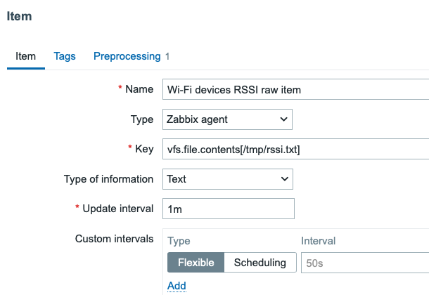
First, I added a new template, for which I then added a new master item reading the /tmp/rssi.txt file.
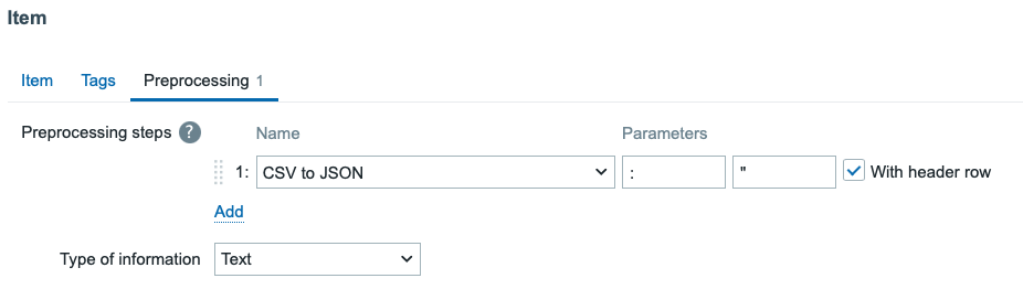
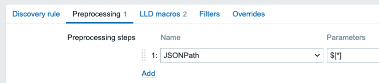
Because ChatGPT script did make the output in CSV format with : as delimiter, we can use Zabbix item preprocessing to convert that CSV to JSON. The JSON output looks like this.
With this, we can then use Zabbix low-level discovery to automatically create the items.
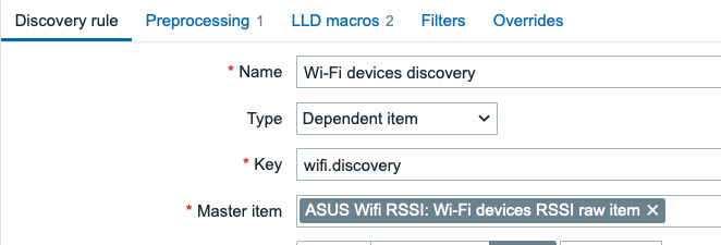
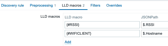
Discovery rule
Now that we have our master item, let’s add the discovery rule, which can go through the JSON. The discovery rule uses my previous item as a dependent item, from which it can parse everything in one go.
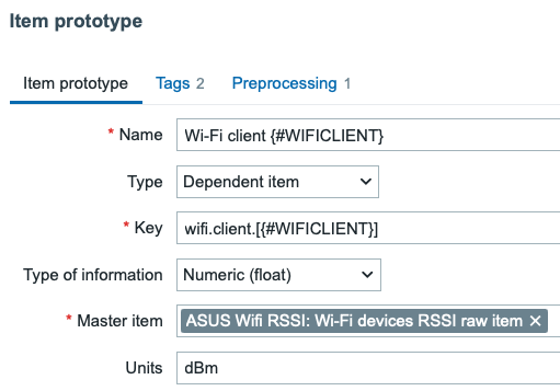
Discovery item prototype
In item prototype, let’s make it again use the raw list as a dependent item and go from there.
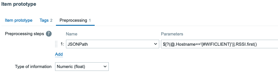
Then in preprocessing, it picks the RSSI value for whatever device LLD was going through by using a JSONPath query…
…or as text:
$[?(@.Hostname=='{#WIFICLIENT}’)].RSSI.first()
That’s pretty much it!
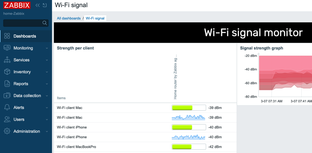
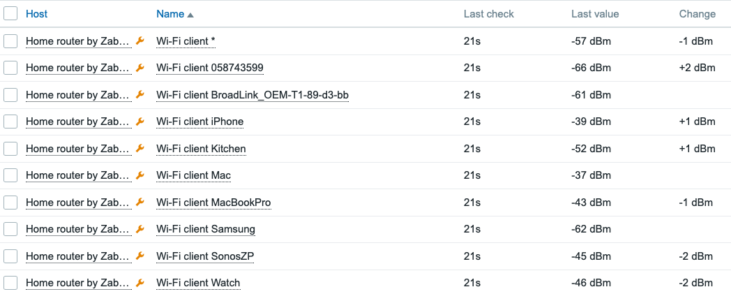
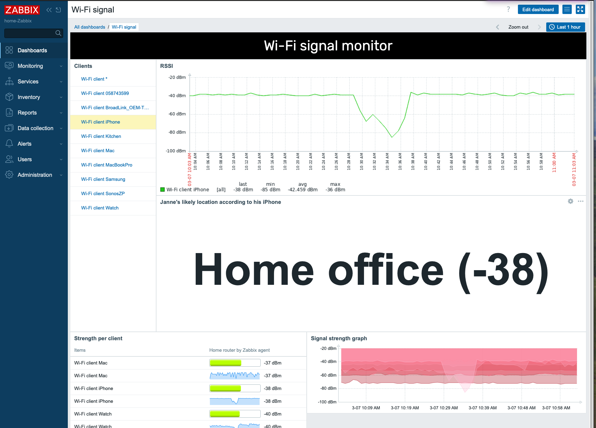
We now have the data coming in once per minute:
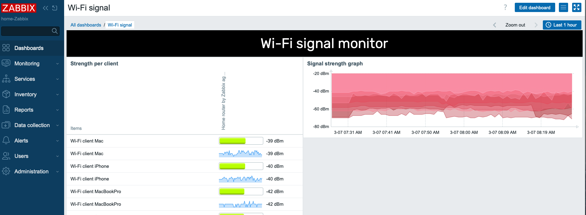
Here’s a little dashboard, too. It shows you the traditional bar that’s available on the Top hosts/items widget, and also the new Sparkline that’s on Zabbix 7.2.
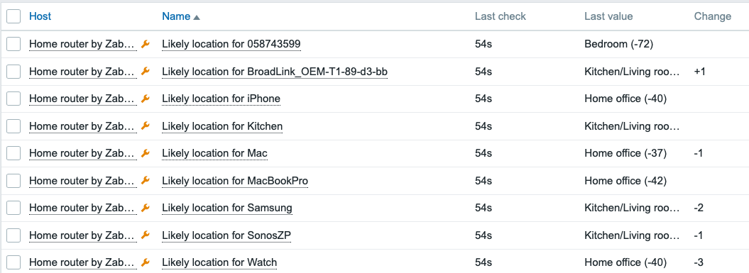
Bonus: Location estimation
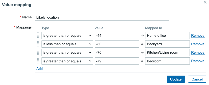
After a little bit of walking around and observing the devices, I added some value mapping to make Zabbix estimate where the devices would be located. It’s not so useful for static objects, but when I move around with my Apple Watch and iPhone, I could make an attempt to monitor my location at home, too.
After this fine-tuning, my dashboard now looks like this:
Thanks for reading, and have fun conducting your own experiments!
Today, after more than 13 years at the company, I am joining Cloudflare’s board of directors and retiring from my full-time position as CTO.
Back in 2012 I wrote a short post on my personal site simply titled: Programmer. The post announced that I’d recently joined a company called CloudFlare (still sporting that capital “F”) with the job title Programmer. I’d chosen that title in part because it was the very first title I’d ever had, and because it would reflect what I’d be doing at Cloudflare.
I had spent a lot of time working at startups—in technical and then management roles—and wanted to go back to the really technical part that I loved most. Cloudflare gave me that opportunity, and I worked on a lot of systems that make up the Cloudflare that so many people around the world use today.
The night we finished the preparation to launch Universal SSL sticks in my memory. We set out to offer the Industry’s First Universal SSL for free, effectively doubling the size of the encrypted web overnight, a big deal in 2014. I remember Cloudflare’s third co-founder, Lee Holloway, hunched over his laptop finishing the code. The team has been working on it all weekend, and late that Sunday night Lee announced “it’s done.”
Handling adversity
It’s easy to pick moments of great success or when things went really well and Cloudbleed in 2017 may not seem like a special moment, but it helped show who we were. It showed how a team could come together under intense stress, and how we could set the standard going forward for how companies disclose and talk about security problems. I personally discovered that a Google Meet call can be kept running for 24 hours and sleeping in two hour chunks is possible.
Being international and intentional
Originally from the UK, I was the first team member located outside the United States. I got to help build the largest offices outside the US: first, Cloudflare’s London office and then Cloudflare’s Lisbon office. These two offices are a big part of who we are today, with Lisbon being our European HQ.
When COVID halted our in-office work, I was blown away by the response from the team. As we all individually faced different difficulties because of the pandemic we continued to work together to ensure that the Internet, on which everyone was relying while confined at home, worked reliably and securely.
Truly impactful technology
Picking a favourite product would be a bit like asking someone to choose their favourite child, but I have soft spots for Cloudflare’s WAF, DNS, and DDoS solutions because I personally worked on those systems. And I still feel I need to apologize to the WAF team who took over my code and had to face that one Perl script that shall not be named!
Beyond the products there’s something much deeper: Cloudflare’s mission to help build a better Internet. I’ve been very proud of how we have supported and advanced the Internet itself through our work on the latest standards and protocols. And I’m even prouder of the role we’ve played through Project Galileo, The Athenian Project, and Cloudflare for Campaigns.
The people
Every week Cloudflare holds an all-hands company meeting which ends with “Shoutouts,” a chance to recognize members of the team who have gone above and beyond. Curiosity and empathy are two core values at Cloudflare, and I am struck every week by how often we’re recognizing teams of people who are being thanked for helping with a sale, fixing a bug, responding to an incident, or helping build Cloudflare. That team spirit is part of what makes Cloudflare a special place to work.
One of the things I will miss about not being at Cloudflare day-to-day is the incredible strength of the individual team members. I’ve been learning from them for 13 years straight!
What’s next
When I joined the company the team was a lot smaller! We were 25 people and now, we’ve grown to more than 4,200 employees and 15 locations across the globe. As we grew I wore a lot of different hats. For a time I ran engineering, operations, security, and even IT. And, of course, I wrote for, and edited, the Cloudflare Blog for many, many years. Over time, we hired many great leaders to run those teams.
But the role that persisted was CTO. And today, we are announcing that, just as I gave up the title Programmer (and the programming that went along with it), I am giving up the title CTO (and the role’s responsibilities) for a new way to help Cloudflare grow and succeed, as a member of the board of directors.
Last year when I told Matthew that I planned to retire, I had not expected to be offered a seat on the company’s board. It’s an incredible and rare honour to go from being an employee of the company (albeit one who has been there from close to the beginning) to joining the board of directors. I am absolutely thrilled to be able to continue helping Cloudflare grow and succeed from a slightly different vantage point.
At the same time, Dane Knecht, who, until today, was SVP of Emerging Technology and Incubation, has become our CTO. Dane joined just a few months after me, and is uniquely positioned and experienced to take the CTO role. We’ve worked so closely for the last 13 years as peers, that in many meetings it would’ve been hard to distinguish our roles. I’m pretty sure that Dane bleeds Cloudflare orange, and I’ve never seen him wear a T-shirt that doesn’t say Cloudflare on it. He has been part of nearly every major milestone here at Cloudflare. He cares so deeply about the company, and its success; he will make a great CTO.
My plan isn’t to go off and work somewhere else, or start a new company. I intend to remain closely involved with Cloudflare in my role on the board. I am incredibly honoured, and grateful to have been part of Cloudflare’s incredible growth and success, and I am looking forward to helping the company continue its growth.
One area I’m particularly interested in assisting with is the company’s work across the product suite on AI. Back in 2002 (23 years ago! gulp!). I wrote a very popular open source machine learning (didn’t call it AI back then) email filtering program and in 2004 worked on how to deal with what happens when one AI system is used to attack another. At Cloudflare, we’ve used learning techniques to enhance security, block bots, and predict how our systems should behave and grow. There’s much more to do.
Just as co-founder Michelle likes to say: we’re just getting started. And so am I.
As AI and machine learning (AI/ML) become increasingly accessible through cloud service providers (CSPs) such as Amazon Web Services (AWS), new security issues can arise that customers need to address. AWS provides a variety of services for AI/ML use cases, and developers often interact with these services through different programming languages. In this blog post, we focus on Python and its pickle module, which supports a process called pickling to serialize and deserialize object structures. This functionality simplifies data management and the sharing of complex data across distributed systems. However, because of potential security issues, it’s important to use pickling with care (see the warning note in pickle — Python object serialization). In this post, we’re going to show you ways to build secure AI/ML workloads that use this powerful Python module, ways to detect that it’s in use that you might not know about, and when it might be getting abused, and finally highlight alternative approaches that can help you avoid these issues.
Quick tips
Avoid unpickling data from untrusted sources
Use alternative serialization formats, when possible, such as Safetensors
Implement integrity checks for serialized data
Use static code analysis tools to detect unsafe pickling patterns, such as Semgrep
Understanding insecure pickle serialization and deserialization in Python
Effective data management is crucial in Python programming, and many developers turn to the pickle module for serialization. However, issues can arise when deserializing data from untrusted sources. The Python bytestream that pickling uses, is proprietary to Python. Until it’s unpickled, the data in the bytestream can’t be thoroughly evaluated. This is where security controls and validation become critical. Without proper validation, there’s a risk that an unauthorized user could inject unexpected code, potentially leading to arbitrary code execution, data tampering, or even unintended access to a system. In the context of AI model loading, secure deserialization is particularly important—it helps prevent outside parties from modifying model behavior, injecting backdoors, or causing inadvertent disclosure of sensitive data.
Throughout this post, we will refer to pickle serialization and deserialization collectively as pickling. Similar issues can be present in other languages (for example, Java and PHP) when untrusted data is used to recreate objects or data structures, resulting in potential security issues such as arbitrary code execution, data corruption, and unauthorized access.
Static code analysis compared to dynamic testing for detecting pickling
Security code reviews, including static code analysis, offer valuable early detection and thorough coverage of pickling-related issues. By examining source code (including third-party libraries and custom code) before deployment, teams can minimize security risks in a cost-effective way. Tools that provide static analysis can automatically flag unsafe pickling patterns, giving developers actionable insights to address issues promptly. Regular code reviews also help developers improve secure coding skills over time.
While static code analysis provides a comprehensive white-box approach, dynamic testing can uncover context-specific issues that only appear during runtime. Both methods are important. In this post, we focus primarily on the role of static code analysis in identifying unsafe pickling.
Tools like Amazon CodeGuru and Semgrep are effective at detecting security issues early. For open source projects, Semgrep is a great option to maintain consistent security checks.
The risks of insecure pickling in AI/ML
Pickling issues in AI/ML contexts can be especially concerning.
Invalidated object loading: AI/ML models are often serialized for future use. Loading these models from untrusted sources without validation can result in arbitrary code execution. Libraries such as pickle, joblib, and some yaml configurations allow serialization but must be handled securely.
For example: If a web application stores user input using pickle and unpickles it later with no validation, an unauthorized user could craft a harmful payload that executes arbitrary code on the server.
Data integrity: The integrity of pickled data is critical. Unexpectedly crafted data could corrupt models, resulting in incorrect predictions or behaviors, which is especially concerning in sensitive domains such as finance, healthcare, and autonomous systems.
For example: A team updates its AI model architecture or preprocessing steps but forgets to retrain and save the updated model. Loading the old pickled model under new code might trigger errors or unpredictable outcomes.
Exposure of sensitive information: Pickling often includes all attributes of an object, potentially exposing sensitive data such as credentials or secrets.
For example: An ML model might contain database credentials within its serialized state. If shared or stored without precautions, an unauthorized user who unpickles the file might gain unintended access to these credentials.
Insufficient data protection: When sent across networks or stored without encryption, pickled data can be intercepted, leading to inadvertent disclosure of sensitive information.
For example: In a healthcare environment, a pickled AI model containing patient data could be transmitted over an unsecured network, enabling an outside party to intercept and read sensitive information.
Performance overhead: Pickling can be slower than other serialization formats (such as, JSON or Protocol Buffers), which can affect ML and large language model (LLM) applications when inference speed is critical.
For example: In a real-time natural language processing (NLP) application using an LLM, heavy pickling or unpickling operations might reduce responsiveness and degrade the user experience.
Detecting unsafe unpickling with static code analysis tools
Static code analysis (SCA) is a valuable practice for applications dealing with pickled data, because it helps detect insecure pickling before deployment. By integrating SCA tools into the development workflow, teams can spot questionable deserialization patterns as soon as code is committed. This proactive approach reduces the risk of events involving unexpected code execution or unintended access due to unsafe object loading.
For instance, in a financial services application where objects are routinely pickled, a SCA tool can scan new commits to detect unvalidated unpickling. If identified, the development team can quickly address the issue, protecting both the integrity of the application and sensitive financial data.
Patterns in the source code
There are various ways to load a pickle object in Python. In this context, methods for detection can be tailored for secure coding habits and needed package dependencies. Many Python libraries include a function to load pickle objects. An effective approach can be to catalog all Python libraries used in the project, then create custom rules in your static code analysis tool to detect unsafe pickling or unpickling within those libraries.
CodeGuru and other static analysis tools continue to evolve their capability to detect unsafe pickling patterns. Organizations can use these tools and create custom rules to identify potential security issues in AI/ML pipelines.
Let’s define the steps for creating a safe process for addressing pickling issues:
Generate a list of all the Python libraries that are used in your repository or environment.
Check the static code analysis tool in your pipeline for current rules and the ability to add custom rules. If the tool is capable of discovering all the libraries used in your project, you can rely on it. However, if it’s not able to discover all the libraries used in your project, you should consider adding user-provided custom rules in your static code analysis tool.
Most of the issues can be identified with well-designed, context-driven patterns in the static code analysis tool. For addressing the pickling issues, you need to identify pickling and unpickling functions.
Implement and test the custom rules to verify full coverage of pickling and unpickling risks. Let’s identify patterns for a few libraries:
NumPy can efficiently pickle and unpickle arrays; useful for scientific computing workflows requiring serialized arrays. To catch potential unsafe pickle usage in NumPy, custom rules could target patterns like:
import numpy as np
data = np.load('data.npy', allow_pickle=True)
npyfile is a utility for loading NumPy arrays from pickled files. You can add the following patterns to your custom rules to discover potentially unsafe pickle object usage.
import npyfile
data = npyfile.load('example.pkl')
pandas can pickle and unpickle DataFrames using pickle, allowing for efficient storage and retrieval of tabular data. You can add the following patterns to your custom rules to discover potentially unsafe pickle object usage.
import pandas as pd
df = pd.read_pickle('dataframe.pkl')
joblib is often used for pickling and unpickling Python objects that involve large data, especially NumPy arrays, more efficiently than standard pickle. You can add the following patterns to your custom rules to discover potentially unsafe pickle object usage.
from joblib import load
data = load('large_data.pkl')
Scikit-learn provides joblib for pickling and unpickling objects and is particularly useful for models. You can add the following patterns to your custom rules to discover potentially unsafe pickle object usage.
from sklearn.externals import joblib
data = joblib.load('example.pkl')
PyTorch provides utilities for loading pickled objects that are especially useful for ML models and tensors. You can add the following patterns to your custom rule format to discover potentially unsafe pickle object usage.
import torch
data = torch.load('example.pkl')
By searching for these functions and parameters in code, you can set up targeted rules that highlight potential issues with pickling.
Effective mitigation
Addressing pickling issues requires not only detection, but also clear guidance on remediation. Consider recommending more secure formats or validations where possible as follows:
PyTorch
Use Safetensors to store tensors. If pickling remains necessary, add integrity checks (for example, hashing) for serialized data.
pandas
Verify data sources and integrity when using pd.read_pickle. Encourage safer alternatives (for example, CSV, HDF5, or Parquet) to help avoid pickling risks.
scikit-learn (via joblib)
Consider Skops for safer persistence. If switching formats isn’t feasible, implement strict validation checks before loading.
General advice
Identify safer libraries or methods whenever possible.
Switch to formats such as CSV or JSON for data, unless object-specific serialization is absolutely required.
Perform source and integrity checks before loading pickle files—even those considered trusted.
Example
The following is an example implementation that shows safe pickle implementation as a representation of the preceding information.
import io
import base64
import pickle
import boto3
import numpy as np
from cryptography.fernet import Fernet

###############################################################################
# 1) RESTRICTED UNPICKLER
###############################################################################
#
# By default, pickle can execute arbitrary code when loading. Here we implement
# a custom Unpickler that only allows certain safe modules/classes. Adjust this
# to your application's requirements.
#

class RestrictedUnpickler(pickle.Unpickler):
    """
    Restricts unpickling to only the modules/classes we explicitly allow.
    """
    allowed_modules = {
        "numpy": set(["ndarray", "dtype"]),
        "builtins": set(["tuple", "list", "dict", "set", "frozenset", "int", "float", "bool", "str"])
    }

    def find_class(self, module, name):
        if module in self.allowed_modules:
            if name in self.allowed_modules[module]:
                return super().find_class(module, name)
        # If not allowed, raise an error to prevent arbitrary code execution.
        raise pickle.UnpicklingError(f"Global '{module}.{name}' is forbidden")

def restricted_loads(data: bytes):
    """Helper function to load pickle data using the RestrictedUnpickler."""
    return RestrictedUnpickler(io.BytesIO(data)).load()

###############################################################################
# 2) AWS KMS & ENCRYPTION HELPERS
###############################################################################

def generate_data_key(kms_key_id: str, region: str = "us-east-1"):
    """
    Generates a fresh data key using AWS KMS.
    Returns (plaintext_key, encrypted_data_key).
    """
    kms_client = boto3.client("kms", region_name=region)
    response = kms_client.generate_data_key(KeyId=kms_key_id, KeySpec='AES_256')

    # Plaintext data key (use to encrypt the pickle data locally)
    plaintext_key = response["Plaintext"]
    # Encrypted data key (store along with your ciphertext)
    encrypted_data_key = response["CiphertextBlob"]
    return plaintext_key, encrypted_data_key

def decrypt_data_key(encrypted_data_key: bytes, region: str = "us-east-1"):
    """
    Decrypts the encrypted data key via AWS KMS, returning the plaintext key.
    """
    kms_client = boto3.client("kms", region_name=region)
    response = kms_client.decrypt(CiphertextBlob=encrypted_data_key)
    return response["Plaintext"]

def build_fernet_key(plaintext_key: bytes) -> Fernet:
    """
    Construct a Fernet instance from a 32-byte data key.
    Fernet requires a 32-byte key *encoded* in URL-safe base64.
    """
    if len(plaintext_key) < 32:
        raise ValueError("Data key is smaller than 32 bytes; cannot build a Fernet key.")
    fernet_key = base64.urlsafe_b64encode(plaintext_key[:32])
    return Fernet(fernet_key)

###############################################################################
# 3) MAIN LOGIC
###############################################################################

def upload_pickled_data_s3(
    numpy_obj: np.ndarray,
    bucket_name: str,
    s3_key: str,
    kms_key_id: str,
    region: str = "us-east-1"
):
    """
    Pickle a numpy object, encrypt it locally, and upload the ciphertext +
    encrypted data key to S3.
    """
    # 1. Generate data key from KMS
    plaintext_key, encrypted_data_key = generate_data_key(kms_key_id, region)

    # 2. Build Fernet from plaintext data key
    fernet = build_fernet_key(plaintext_key)

    # 3. Serialize the numpy object with pickle
    pickled_data = pickle.dumps(numpy_obj, protocol=pickle.HIGHEST_PROTOCOL)

    # 4. Encrypt the pickled data
    encrypted_data = fernet.encrypt(pickled_data)

    # 5. Upload to S3 along with the encrypted data key (in metadata)
    s3_client = boto3.client("s3", region_name=region)
    s3_client.put_object(
        Bucket=bucket_name,
        Key=s3_key,
        Body=encrypted_data,
        Metadata={
            "encrypted_data_key": base64.b64encode(encrypted_data_key).decode("utf-8")
        }
    )
    print(f"Encrypted pickle uploaded to s3://{bucket_name}/{s3_key}")

def download_and_unpickle_data_s3(
    bucket_name: str,
    s3_key: str,
    region: str = "us-east-1"
) -> np.ndarray:
    """
    Download the ciphertext and the encrypted data key from S3. Decrypt the data
    key with KMS, use it to decrypt the pickled data, then load with a restricted
    unpickler for safety.
    """
    s3_client = boto3.client("s3", region_name=region)

    # 1. Get object from S3
    response = s3_client.get_object(Bucket=bucket_name, Key=s3_key)

    # 2. Extract the encrypted data key from metadata
    metadata = response["Metadata"]
    encrypted_data_key_b64 = metadata.get("encrypted_data_key")
    if not encrypted_data_key_b64:
        raise ValueError("Missing encrypted_data_key in S3 object metadata.")

    encrypted_data_key = base64.b64decode(encrypted_data_key_b64)

    # 3. Decrypt data key via KMS
    plaintext_key = decrypt_data_key(encrypted_data_key, region)
    fernet = build_fernet_key(plaintext_key)

    # 4. Decrypt the pickled data
    encrypted_data = response["Body"].read()
    decrypted_pickled_data = fernet.decrypt(encrypted_data)

    # 5. Use restricted unpickler to load the numpy object
    numpy_obj = restricted_loads(decrypted_pickled_data)

    return numpy_obj

###############################################################################
# DEMO USAGE
###############################################################################

if __name__ == "__main__":
    # --- Replace with your actual values ---
    KMS_KEY_ID = "arn:aws:kms:us-east-1:123456789012:key/your-kms-key-id"
    BUCKET_NAME = "your-secure-bucket"
    S3_OBJECT_KEY = "encrypted_npy_demo.bin"
    AWS_REGION = "us-east-1"  # or region of your choice

    # Example numpy array
    original_array = np.random.rand(2, 3)
    print("Original Array:")
    print(original_array)

    # Upload (pickle + encrypt) to S3
    upload_pickled_data_s3(
        numpy_obj=original_array,
        bucket_name=BUCKET_NAME,
        s3_key=S3_OBJECT_KEY,
        kms_key_id=KMS_KEY_ID,
        region=AWS_REGION
    )

    # Download (decrypt + unpickle) from S3
    retrieved_array = download_and_unpickle_data_s3(
        bucket_name=BUCKET_NAME,
        s3_key=S3_OBJECT_KEY,
        region=AWS_REGION
    )

    print("\nRetrieved Array:")
    print(retrieved_array)

    # Verify integrity
    assert np.allclose(original_array, retrieved_array), "Arrays do not match!"
    print("\nSuccess! The retrieved array matches the original array.")
Conclusion
With the rapid expansion of cloud technologies, integrating static code analysis into your AI/ML development process is increasingly important. While pickling offers a powerful way to serialize objects for AI/ML and LLM applications, you can mitigate potential risks by applying manual secure code reviews, setting up automated SCA with custom rules, and following best practices such as using alternative serialization methods or verifying data integrity.
When working with ML models on AWS, see the AWS Well-Architected Framework’s Machine Learning Lens for guidance on secure architecture and recommended practices. By combining these approaches, you can maintain a strong security posture and streamline the AI/ML development lifecycle.
If you have feedback about this post, submit comments in the Comments section below. If you have questions about this post, contact AWS Support.
Web application owners are constantly working to protect their applications from a variety of threats. Previously, if you wanted to implement a robust security posture for your Amplify Hosted applications, you needed to create architectures using Amazon CloudFront distributions with AWS WAF protection, which required additional configuration steps, expertise, and management overhead.
With the general availability of AWS WAF in Amplify Hosting, you can now directly attach a web application firewall to your AWS Amplify apps through a one-click integration in the Amplify console or using infrastructure as code (IaC). This integration gives you access to the full range of AWS WAF capabilities including managed rules, which provide protection against common web exploits and vulnerabilities like SQL injection and cross-site scripting (XSS). You can also create your own custom rules based on your specific application needs.
This new capability helps you implement defense-in-depth security strategies for your web applications. You can take advantage of AWS WAF rate-based rules to protect against distributed denial of service (DDoS) attacks by limiting the rate of requests from IP addresses. Additionally, you can implement geo-blocking to restrict access to your applications from specific countries, which is particularly valuable if your service is designed for specific geographic regions.
Let’s see how it works Setting up AWS WAF protection for your Amplify app is straightforward. From the Amplify console, navigate to your app settings, select the Firewall tab, and choose the predefined rules you want to apply to your configuration.
Amplify hosting simplifies configuring firewall rules. You can activate four categories of protection.
Amplify-recommended firewall protection – Protect against the most common vulnerabilities found in web applications, block IP addresses from potential threats based on Amazon internal threat intelligence, and protect against malicious actors discovering application vulnerabilities.
Restrict access to amplifyapp.com – Restrict access to the default Amplify generated amplifyapp.com domain. This is useful when you add a custom domain to prevent bots and search engines from crawling the domain.
Enable IP address protection – Restrict web traffic by allowing or blocking requests from specified IP address ranges.
Enable country protection – Restrict access based on specific countries.
Protections enabled through the Amplify console will create an underlying web access control list (ACL) in your AWS account. For fine-grained rulesets, you can use the AWS WAF console rule builder.
After a few minutes, the rules are associated to your app and AWS WAF blocks suspicious requests.
If you want to see AWS WAF in action, you can simulate an attack and monitor it using the AWS WAF request inspection capabilities. For example, you can send a request with an empty User-Agent value. It will trigger a blocking rule in AWS WAF.
Let’s first send a valid request to my app.
curl -v -H "User-Agent: MyUserAgent" https://main.d3sk5bt8rx6f9y.amplifyapp.com/
* Host main.d3sk5bt8rx6f9y.amplifyapp.com:443 was resolved.
...(redacted for brevity)...
> GET / HTTP/2
> Host: main.d3sk5bt8rx6f9y.amplifyapp.com
> Accept: */*
> User-Agent: MyUserAgent
>
* Request completely sent off
< HTTP/2 200
< content-type: text/html
< content-length: 0
< date: Mon, 10 Mar 2025 14:45:26 GMT
We can observe that the server returned an HTTP 200 (OK) message.
Then, send a request with no value associated to the User-Agent HTTP header.
 curl -v -H "User-Agent: " https://main.d3sk5bt8rx6f9y.amplifyapp.com/
* Host main.d3sk5bt8rx6f9y.amplifyapp.com:443 was resolved.
... (redacted for brevity) ...
> GET / HTTP/2
> Host: main.d3sk5bt8rx6f9y.amplifyapp.com
> Accept: */*
>
* Request completely sent off
< HTTP/2 403
< server: CloudFront
... (redacted for brevity) ...
<TITLE>ERROR: The request could not be satisfied</TITLE>
</HEAD><BODY>
<H1>403 ERROR</H1>
<H2>The request could not be satisfied.</H2>
We can observe that the server returned an HTTP 403 (Forbidden) message.
AWS WAF provide visibility into request patterns, helping you fine-tune your security settings over time. You can access logs through Amplify Hosting or the AWS WAF console to analyze traffic trends and refine security rules as needed.
Availability and pricing Firewall support is available in all AWS Regions in which Amplify Hosting operates. This integration falls under an AWS WAF global resource, similar to Amazon CloudFront. Web ACLs can be attached to multiple Amplify Hosting apps, but they must reside in the same Region.
The pricing for this integration follows the standard AWS WAF pricing model, You pay for the AWS WAF resources you use based on the number of web ACLs, rules, and requests. On top of that, AWS Amplify Hosting adds $15/month when you attach a web application firewall to your application. This is prorated by the hour.
This new capability brings enterprise-grade security features to all Amplify Hosting customers, from individual developers to large enterprises. You can now build, host, and protect your web applications within the same service, reducing the complexity of your architecture and streamlining your security management.
(This survey is hosted by an external company. AWS handles your information as described in the AWS Privacy Notice. AWS will own the data gathered via this survey and will not share the information collected with survey respondents.)
Amazon Web Services (AWS) is pleased to announce that the Winter 2024 System and Organization Controls (SOC) 1 report is now available. The report covers 183 services over the 12-month period from January 1, 2024, to December 31, 2024, giving customers a full year of assurance. This report demonstrates our continuous commitment to adhere to the heightened expectations for cloud service providers.
AWS strives to continuously bring services into the scope of its compliance programs to help customers meet their architectural and regulatory needs. Customers can reach out to their AWS account team if they have any questions or feedback about SOC compliance.
To learn more about AWS compliance and security programs, see AWS Compliance Programs. As always, we value feedback and questions; reach out to the AWS Compliance team through the Contact Us page.
If you have feedback about this post, submit comments in the Comments section below.
For a long time, we have been focusing a lot on the hardware costs of new processors but missing the virtualization license costs. Part of that is simply due to the number of virtualization licenses and support models. Recently, we purchased the most popular barebones server and the most popular server processor on Newegg to […]
Понякога да направят своя материал им отнема един месец, понякога – шест години. Двамата се срещат с хора и през личното успяват да стигнат до по-големия разказ – за региона, процесите или духа на времето. И макар близо до прословутия Zeitgeist, уловеното от тях няма предвид пряко културния или политическия климат за съответния момент, но в контекста улавя тъкмо тях.
Димитър и Александър изминават хиляди километри за всяка своя история, разговарят с различни хора, нерядко успяват да задействат и обществена енергия, за да помогнат. Не защото сляпо вярват в силата на журналистиката, а защото са се научили да виждат и със сърцето си. Снимките и дизайнът на платформата им позволяват на читателя също да съпреживява, докато скролва движещия се върху фотографиите текст. В отскоро преобразения им подкаст човек може да чуе и непосредствен разговор между двамата за предизвикателствата, нелепите моменти и трудностите на терен или поне да научи институция ли е водомайсторът, или магически персонаж.
Димитър Панайотов (журналист) и Александър Николов (фотограф) са хората, които създават мултимедийна документалистика от нов тип. Запознават се във форум за фотография и всичко започва като мечта, трансформира се неколкократно, обединявайки методологиите на журналистиката и документалното разказване. И ето ги тук и сега, 10 години по-късно те пускат „на вода“ новата си медийна платформа „Ден“, в която ежемесечно представят по една социалнозначима история.
Последният им експериментален разказ е за Добруджа и върви по стъпките на Йовковата проза. Пътищата в старата житница на България все още възвиват към морето – заради онзи живот отпреди сто години, когато най-важен за тукашната икономика е бил скеля (пристанището) в Балчик. Минават през села, в които не е останало нито едно дете, но местните краеведи записват и съхраняват истории. В село Змеево, казват Димитър и Александър, все още има кой да ти покаже Антимовския хан.
В историята за преселенията в Добруджа се оглеждат и днешните ни битки за хуманност и нормалност. Но и онтологията на стари вражди – отколешното недоверие, с което приемаме „преселеца“, другия. Да припознаваме враг във всеки непознат, дори в децата от преселнически семейства, които са се родили и израснали в България – навярно тук се корени част от българската провинциалност, колкото съхранителна, толкова и душна, спарена, недопускаща.
Дългогодишната отдаденост на документалистиката на Димитър и Александър от „Ден“ е опит да бъдем човешки адекватни и граждански съпричастни. Издател на медията им е собствената им фондация „Документалистите“ – не се сещам за по-точно име в техния случай.
Да имаш време за каузите и идеите си ли е най-големият лукс днес?
Димитър: Според мен е лукс, защото живеем във време, в което всичко е много бързо. Това, което ние правим, е опит за социална промяна и активизъм чрез бавна документалистика и задълбочена журналистика. Изисква да се отдадеш, да отделиш време, изисква да активираш мозъка си – както да създадеш крайния продукт, така и като читател да го прочетеш и осмислиш. Не знам дали хората си дават сметка – със сигурност не, а и не трябва, – но една статия обикновено е между 3000 и 5000 думи, което е голям обем за нашето време, но не е чак толкова дълго [за четене – б.р.]. Тя обаче отнема месеци, понякога и години, но във всеки случай най-малко няколко седмици, за да бъде създадена. Много часове са нужни за предварително проучване, след това отиваме на терен. Там е най-сложно, но и най-вълнуващо, понякога имаме 16-часови снимачни дни.
Този огромен обем от информация, който сме събрали, после обсъждаме с консултанти, защото ние няма как да сме експерти по бежанската криза, по донорството или безводието. Затова винаги вземаме едни от най-добрите и реномирани консултанти в областта.
После Сашо обработва снимките и създава мултимедията, която само ние правим. Никой в България не ползва този формат, който е интерактивен и мултимедиен. Всяка отделна история има свой дизайн, специално правен на ръка за нея конкретно.
Александър: От една страна, е лукс за нас да можем да си позволим наистина да правим това, което много харесваме и обичаме. И от друга страна, е лукс за потребителя, който трябва да отдели от ценното си време и да прочете и преживее това, което правим.
Ако трябва да сте фундаменталисти или радикални, в коя сфера бихте били?
Димитър: Чувството за справедливост, защото справедливостта е нещо, което не съществува като физичен закон, тя е измислена от нас, хората, от нашия морал. За съжаление, има всякакви видове несправедливост. Аз съм абсолютен радикал на тема справедливост. Второто нещо са истината и фактите. Защото живеем във време, в което истината и фактите се тълкуват по всякакви начини. От един от моите преподаватели научих, че в журналистиката двете гледни точки не във всеки случай съществуват. Не можеш да покажеш в телевизионно студио двама души, които да спорят дали навън вали. Не може да има две мнения за това, при положение че през прозореца се вижда вали ли. Тук не става въпрос да не спорим за политика или геополитика, религия, възгледи, принципи. А за чистите факти. Не за абстракции. Напоследък виждаме как се изопачава истината по всякакви начини, от всички страни.
Александър: Каквото и да правим, с каквото и да се занимаваме, на първо място абсолютно винаги сме хора. Трябва да уважаваме хората, трябва да ги разбираме и да подхождаме човешки. Има една много известна снимка на умиращо дете и лешояд – на фотографа Кевин Картър. В тази ситуация ние не оставяме детето да умре, не сме пасивни наблюдатели. Защото ценим човешкия живот, човешкото достойнство и човешките права като цяло.
Но да резюмирам и за фактите. Ние държим на тях. Например когато събарят ромски къщи, не можем да кажем, че тези къщи не са незаконни – те са незаконни. Това е факт, но винаги може да покажем човешката емоция и да попитаме защо властимащите и държавните структури са позволили тези къщи да съществуват. И дори са им отворили партиди за ток и вода. А в момента правят нещо, което ще остави стотици хора на улицата. Това може да бъде голям проблем за града – просто да махнем къщите. Защото къде отиват хората?
Какво пазите в архивите на въображението?
Димитър: Сблъскваме се с най-различни теми, произлизащи от хората, които срещаме на терен, от разговорите помежду ни или с наши приятели. Представяме си как могат да бъдат направени, какво въздействие могат да имат върху нас като автори и върху аудиторията, започваме да мечтаем някой ден да ги реализираме по възможно най-добрия начин.
Александър: Една от историите ни беше провокирана от факта, че брат ми стана донор на органи на 21 години. Това се превърна в тема, която отне голяма част от младостта ни. Открихме, че искаме да работим заедно и да разказваме истории по нов начин, като всеки допринесе с това, което може. Например, погледнато от моята камбанария, снимките да не са просто илюстрация на даден текст, а да носят допълнителни смислови слоеве, да могат да доразвиват историята. Димитър се шегува с мен, че голяма част от историите, които разказваме, са свързани със семейството. Например село Гурково, което е една от локациите ни по темата за Йовковата Добруджа – реално там имахме добра входна точка, защото дядо ми и баба ми, които са се заселили в Гурково, са мигранти, били са изселени от Северна Добруджа.
Димитър:Ние малко сме смесили личния живот с нашата работа, даже много трудно обясняваме на хората какво точно работим. Често го правим заедно с приятели. Например с Пламена Крумова – моя близка приятелка, с която сме съученици, после колеги – работим заедно по всички проекти, тя ни поддържа социалните мрежи. С приятели направихме и кампанията за донорство.
Хората около нас се запалват по темите и са съпричастни, помагат ни. Това, с което се занимаваме, е съществена част от живота ни. Били сме изморени, бърнаутвали сме, пътуваме много, но въпреки всичко продължаваме, защото това, което правим, ни кара да се чувстваме смислени – кара ни да горим.
Така се случи, че ние сме софийска фондация, но всъщност реално нямаме софийска история.
Писали сме по много теми, все пак сме професионални журналисти, знаем какво да правим на терен, работейки по социални и тежки теми. Аз съм по-директен, Сашо е много по-мек, по-обран. И двамата обаче сме много искрени, обясняваме какво правим, показваме какво сме направили дотук и каква ни е целта. Добронамерени сме, не правим разследваща журналистика, но не си затваряме очите за проблемите.
Хората, с които говорим, винаги са скептични в началото. Но спечелваме доверието им, често ставаме добри познати и дори приятели с герои от наши материали.
Александър: Именно защото винаги сме искрени, не прикриваме нещо. Хората ни се доверяват, защото разбират какво правим, може би не сме застрашителни, допускат ни.
Виждате ли връзка между документалистиката и емпатията?
Димитър: Много е важна! Аз пиша и влизам в нещата емоционално, докато Александър е по-рационален външно. Понякога аз прекалявам с емоцията, но той добавя баланс, рита ме под масата, докато говорим с някого.
Александър: Ако не се поставиш в обувките на този, с когото говориш, няма как да спечелиш доверието му, да го накараш да ти разкаже историята си и после да го снимаш. Няма начин без емпатия да го разкажеш такъв, какъвто е.
Димитър: В нашите текстове има рефлексия, включително авторефлексия. Примерно, в мултимедийните ни истории – всяка от тях си има героите, обаче всъщност главните разказвачи сме аз и Александър: той – със снимките, аз – с текст.
Александър: Ние все пак, в дъното, говорим за човешките права и за сериозни социални и екологични проблеми. Дали ще е през Йовков, или ще става дума за селата в района на Омуртаг, или за ромската махала от Стара Загора, ние говорим по социални теми.
Искам да кажа и за тъмната страна на емпатията обаче – когато работиш, се сблъскваш с истории, които са тежки житейски и човешки. Това няма как да не ти се отрази психически. И все пак трябва да намираме някакви механизми, с които след тези срещи, дори понякога и по време на разговорите, да успяваме да се самосъхраним. Защото когато се отдадеш напълно, нещата, които чуваш, се превръщат в неотработени травми. Ти ги преживяваш.
Снимки по темата за трансплантациите. Личен архив на Димитър Панайотов и Александър Николов
Димитър:Вече имаме много механизми и начини, по които се справяме с тежките истории и картини, които виждаме на терен. Но това го научихме по трудния начин. На много млада възраст видяхме брутални неща, които хората не трябва да виждат – операции, трансплантации, майчини сълзи, скръб и смърт. При мен тогава се отключи сериозна тревожност. Възможно е тя да е била в отговор и на неща от личния ми живот. Докато аз си го изкарах с паника и тревожност, Сашо си го отработваше интровертно с някакви свои мисли. Отне ни години да се справим с всичко това. Във всеки случай обаче, научихме се да плуваме директно в дълбокото.
Александър: Но и до днес ни е трудно в следващите няколко дни, след като сме снимали тежки истории.
Вие бяхте на границата още в първата седмица на войната в Украйна. С какви цветове, миризми, звуци асоциирате първите дни на бежанската вълна?
Александър: Мирисът на урина ми остана много, много силно. Когато се прибирахме, взехме едно украинско семейство от Румъния, с малко момиченце, около 2–3 годишно, и то се напишка. И ето, мирисът е нещото, което ми е останало в съзнанието, макар това да не сме го писали никъде.
Иначе, чисто емоционално, всичко това виждаме и сега, след трагедията в Северна Македония – как хората, независимо от своята националност, пол или раса, могат да се обединят. И да работят заедно, да загърбят всички пререкания помежду си, всички политически разбирания, всички предразсъдъци. И наистина да работят за нещо по-висше от тях.
Украински бежанци. Личен архив на Димитър Панайотов и Александър Николов
Димитър: Останало ми е цветовото усещане за сиво и червено. Сиво – защото след началото на войната първото нещо, което видях, когато отворих лаптопа си, бяха димните кълба от Киев. Освен това времето беше сиво и мрачно през февруари и началото на март.
Но и червеното – като жилетките на спасителите. И като надежда.
Това беше от най-силните теми, нещо, което никога не се е случвало в нашия живот. Имаше много динамика, ние не бяхме там, докъдето стигна войната, снимахме Румъния и България и въпреки огромната болка, страдание, мъка, това беше от моментите, в които съм вярвал най-силно в човечеството.
Аз не съм предполагал, че българи и румънци могат да реагират по този начин. Всички хора помагаха и даряваха, имаше опашки от доброволци. В Несебър свещеникът отвори църквата за бежанците, навсякъде имаше много надежда, взаимопомощ. И нямаше нищо общо с разделението и омразата, която е в момента. На чисто импулсивно, първично ниво всички реагирахме много човешки. Това се разми с годините, сега остана чисто политическото. И стигнахме до онова клише, че смъртта на един милион човешки същества е статистика. Сега говорим за тази Украйна, все едно е някакъв обект.
Тогава впрочем много спонтанно ни хрумна на мен и Александър, че можем ефикасно да съчетаваме журналистика с активизъм. Ние всъщност си бяхме доброволци активисти, събирахме дарения, купувахме храна и лекарства, карахме хора към границата, взехме семейството на един руснак, който беше и още е женен за украинка. След това на връщане взехме украинка заедно с малкото ѝ момиче и възрастна майка и им намерихме хотел да отседнат безплатно – и това ставаше след полунощ.
Какви са вашите малки спасителни бягства днес?
Александър: Моето е наистина теренната работа, защото тогава аз лично бягам от натовареното ежедневие. Освен че сме създатели на съдържание и концепции, ние имаме и много, много административна работа, която трябва да се свърши. В семейството – също. И буквално си е малко бягство от ежедневието да отидеш на непознато място, където ще срещаш интересни хора и история.
Димитър: С любимата, най-добре на път, много обичаме да караме към всякакви дестинации. С хубава книга или филм. И една добра тренировка с тежести.
Физическото движение – сега си припомних отново колко фундаментално важно е не само за здравето и за фигурата, а и за менталното състояние. Защото ние не просто полагаме интелектуален труд, естествено, ние сме преди всичко журналисти, но сме и милион други неща – отчитаме проекти, оправяме счетоводство, менажираме екипи от хора.
Спортът и пътят се оказаха най-добрият ескейпизъм за мен.
Version
0.11 of the Neovim text editor has been released. Notable changes
in this release include simpler Language Server Protocol (LSP) client
setup, improved tree-sitter performance, better emoji support, and
enhancements for Neovim’s embedded terminal emulator. See the release notes for
a full list of changes.
Rapid7 has been honored by CRN®, a brand of The Channel Company, with a 5-Star Award in the 2025 CRN Partner Program Guide. This annual guide is an essential resource for solution providers seeking vendor partner programs that match their business goals and deliver high partner value.
Recognition of Rapid7’s continued commitment to channel
The 5-Star Award is an elite recognition given to companies that have built their partner programs on the key elements needed to nurture lasting, profitable, and successful channel partnerships
When evaluating potential collaborations with IT vendors, Partners must carefully consider the comprehensive support and resources offered through vendors’ partner programs. Key program components, including financial incentives, sales and marketing support, training and certification, and technical assistance – can significantly distinguish vendors such as Rapid7. These elements are instrumental in enhancing the long-term growth and profitability of their partnerships.
For the 2025 Partner Program Guide, the CRN research team evaluated vendors based on program requirements and offerings such as partner training and education, pre- and post-sales support, marketing programs and resources, technical support, and communication. Rapid7 acknowledges the significance of these critical program features and is pleased to have integrated all of these elements into the 2025 PACT program.
Aligned with our recent program launch
This prestigious recognition closely follows the introduction of the enhanced 2025 PACT Partner Program. Rapid7 recognizes that in today’s increasingly complex threat landscape, partners face mounting pressure to have access to the tools, training, and resources necessary to meet the expanding security demands of their clients. Rapid7 is strategically positioned to fulfill these essential partner needs, having launched the revitalized Partner Program PACT 2025. This comprehensive program is designed to represent and support our expanding community of partners – encompassing diverse business models – all unified under a cohesive framework with competitive benefits and partnership support.
Being featured in the 2025 CRN Partner Program Guide highlights the dedication these technology vendors have to evolving with solution providers, driving innovation, and supporting mutual success,” said Jennifer Follett, VP, U.S. Content and Executive Editor, CRN, at The Channel Company. “This critical annual project empowers solution providers to identify vendors that are committed to enhancing their partner programs and meeting the always-changing business needs of the channel and end customers. The guide provides deep insight into the distinctive value of each partner program so solution providers can make strategic partnership decisions with confidence.”
Future outlook: Sustained focus and commitment
Our dedication to our partners is unwavering, as we continue to engage collaboratively with our global partner network. We are committed to understanding the needs of our partners as well as addressing business challenges and opportunities.
We will continue to develop strategies that improve the ease and efficiency of our business engagements, ensuring exceptional experiences and exemplifying our partner-first culture. Our programs are developed in collaboration with our partners, and maintaining a continuous feedback loop is essential as we work to evolve and enhance our offerings.
Every organization strives to empower teams to drive innovation while safeguarding their data and systems from unintended access. For organizations that have thousands of Amazon Web Services (AWS) resources spread across multiple accounts, organization-wide permissions guardrails can help maintain secure and compliant configurations. For example, some AWS services support resource-based policies that can be used to grant identities permissions to perform actions on the resources they’re attached to. With the management of resource-based policies frequently delegated to application owners, central security teams use permissions guardrails to help ensure that possible misconfigurations don’t lead to unintended access to these resources.
In this post, we discuss how you can use resource control policies (RCPs) to centrally restrict access to resources. We demonstrate how RCPs can help improve your security posture while allowing even more freedom to developers in managing their resources, thus reducing friction between central security and application teams. Using a sample use case, we uncover key considerations for designing and effectively implementing RCPs in your organization at scale.
We recommend implementing permissions guardrails, including RCPs, using the following iterative process, which consists of five phases (as shown in Figure 1).
This phased approach helps ensure an effective integration of RCPs into your security strategy, improving your security posture while helping to maintain business continuity. Let’s explore each phase of RCP implementation in detail and outline key considerations for an effective implementation strategy.
Phase 1: Examine your security control objectives
The first step in implementing RCPs is identifying areas where RCPs can help improve your security posture or optimize the implementation of controls for your organization’s specific security control objectives.
Your control objectives can be influenced by a variety of factors such as compliance and regulatory requirements, legal and contractual obligations, types of workloads, data classification, and your organization’s threat model. After your control objectives are well-defined and prioritized, identify those that can be achieved using RCPs.
Like SCPs, RCPs are designed to establish coarse-grained access controls, security invariants that rarely change and serve as always-on boundaries across a wide range of AWS resources in your accounts. RCPs aren’t for managing fine-grained access controls. You will keep using policies such as resource-based and identity-based policies to apply least-privilege permissions.
More specifically, the following are key control objectives that you can achieve using RCPs:
Establish a data perimeter around your AWS resources. For example, you can use RCPs to help ensure that only trusted identities can access your AWS resources.
Mitigate the cross-service confused deputy risk. You can use RCPs to help ensure that your AWS resources are accessed by AWS services only on behalf of your organization.
Apply consistent access controls to your AWS resources regardless of the identities accessing them. For example, you can use RCPs to help ensure your Amazon Simple Storage Service (Amazon S3) buckets require TLS v1.2 or higher for in-transit encryption.
Let’s begin with the scenario illustrated in Figure 2. Your company’s central cloud team manages your corporate AWS Organizations organization, which consists of two corporate AWS accounts. An IAM principal in Account A should be able to assume an IAM role in Account B to perform day-to-day operations. To align to the broader control objective of Only trusted identities can access my resources, the central security team wants to make sure that the IAM role in Account B (my resource) can only be assumed by IAM principals that belong to their organization (trusted identities).
Figure 2: Simple scenario depicting a trusted identity accessing an IAM role
One way of achieving this control objective is to follow the principle of least-privilege and make sure that the role trust policy, the resource-based policy attached to the IAM role, only allows access to identities that require that access. The following is an example trust policy that grants permissions to Role A in Account A to assume Role B in Account B.
In organizations that have only a few accounts, central teams typically manage these policies. While this centralized governance model helps ensure that trust policies applied to roles are always restricted to trusted identities, it can also impede the productivity of application teams when operating at a greater scale.
Assume that your company has started growing its cloud footprint so much that your central security team now must achieve the same control objective with hundreds of IAM roles that are spread across multiple AWS accounts, as demonstrated in Figure 3.
Figure 3: Restricting access by managing individual IAM role trust policies
At this scale, we see organizations delegating permissions management to application teams to better support the growth of their business and empower developers to innovate faster. While central security teams no longer have full control over the permissions granted to resources across AWS accounts, they must make sure that access is aligned with their organization’s security standard. For example, they might want to make sure that the GrantCrossAccountAccess statement that is now managed by developers doesn’t inadvertently grant access to an account that doesn’t belong to their organization. Previously, central security teams typically achieved this by developing automated mechanisms to insert a standard statement into all trust policies. This statement helped ensure that access remained bounded to their organization, even when developers configured broad access permissions for their roles. The following is an example trust policy where a developer granted permissions to an external account through the GrantCrossAccountAccess statement. However, because of the RestrictAccessToMyOrg statement added to the policy by the central security team, the external account will be unable to use these permissions.
The RestrictAccessToMyOrg statement uses the aws:PrincipalOrgID and aws:PrincipalIsAWSService condition keys to restrict access to principals within your organization or to AWS service principals. The BoolIfExists operator with the aws:PrincipalIsAWSService condition key is required if the roles you’re applying a control to are service roles that are used by AWS services to perform operations on your behalf. When an AWS service assumes a service role, it uses its AWS service principal, an identity that is owned by AWS and that does not belong to your organization.
The central security teams could, for example, use AWS Config rules to detect misconfigurations and then use AWS Config remediation to automatically add the RestrictAccessToMyOrg statement to the IAM roles’ trust policies when new IAM roles are created or their trust policies are changed. Even though the addition of the RestrictAccessToMyOrg statement to trust policies can be automated, RCPs can greatly simplify enforcement of such coarse-grained controls in a multi-account environment.
Phase 2: Design permissions guardrails
Central security teams can implement permissions guardrails by creating an RCP that centrally blocks external access to IAM roles. The RCP that you will implement contains similar restrictions to the RestrictAccessToMyOrg statement that you used in the IAM trust policy.
Like SCPs, you attach the RCP to an account, organizational unit (OU), or the root of your organization. After being attached, the RCP automatically applies to applicable resources—in this case, IAM roles—within the scope of that AWS Organizations entity. This centralized approach alleviates the need to modify hundreds of trust policies across multiple accounts, lowering the operational overhead for central security teams and helping ensure consistent access controls are applied at scale. RCPs also help you achieve separation of duties with developers still managing their least-privilege permissions in trust policies and administrators applying coarse-grained access controls in RCPs. If developers make configuration mistakes while managing permissions for their applications, the preventative access controls implemented using RCPs will help ensure that they stay within your organization’s access control guidelines. See How AWS enforcement code logic evaluates requests to allow or deny access to understand how different policy types impact the authorization process.
If you’re transitioning existing controls from resource-based policies to RCPs, use the opportunity to reassess the control design based on your current control objectives and the additional benefits offered by RCPs. For example, your previous controls might have been limited to specific resource types, such as IAM roles in this use case, or to particular accounts, such as those storing the most sensitive data. RCPs enable you to extend controls to additional resources across your entire organization, reducing operational overhead through centralized management of permissions guardrails.
While designing your RCPs, consider the following guidelines.
Design for operational excellence
A key foundation for effectively implementing and operating permissions guardrails like RCPs is organizing your AWS environment using multiple accounts. Account boundaries and strategic placement of workloads across them allow you to apply tailored access controls that align with data sensitivity and specific access requirements. Grouping accounts into OUs within AWS Organizations enables more effective access control, even in scenarios where cross-account access is required. Figure 4 illustrates an example organization structure, demonstrating how RCPs can be applied at various levels of the organizational hierarchy to adhere to the security requirements of different workloads.
Figure 4: A sample organization with RCPs applied at various levels
When operating at scale, consider delegating policy management to a central security account in your organization. With AWS Organizations resource-based delegation, central teams don’t need access to the management account for any SCP or RCP related changes or troubleshooting.
Establishing clear governance helps you define how to implement and continuously manage RCPs within your organization. This includes the operating model, change management processes, and exceptions handling procedures. RCPs provide authorization controls similar to SCPs and therefore should integrate with your existing governance framework rather than requiring separate oversight. For example, if your change management process requires two-person approval for SCP changes, you should consider applying the same approval process for RCP implementation. You should also adopt the same mechanisms you currently use to prevent unauthorized changes or detect drifts in your policies.
Plan for exceptions
There might be scenarios where you have a few resources that should be accessible publicly or by identities that don’t belong to your organization. If you’re organizing your resources across multiple accounts and OUs based on their compliance requirements or a common set of controls, then you most likely have such resources in a dedicated set of accounts or OUs, such as the Public Data OU in Figure 4. These accounts or OUs can have applicable policies that account for their unique access requirements.
Another option to accommodate these scenarios is to use the aws:ResourceAccount or aws:ResourceOrgPaths condition key to exclude certain accounts from the control. For example, the following policy will deny access to identities outside your organization from assuming IAM roles unless the identity is an AWS service principal or the role that is being accessed belongs to Account A.
There also might be situations where your company’s trusted partners or acquisitions need to be granted an exception for access to a subset of your company’s resources distributed across multiple accounts. For example, your company might integrate with Cloud Security Posture Management (CSPM) tools that assume roles in your accounts to assess your accounts’ security posture, as shown in Figure 5.
Figure 5: Representative view of granting exceptions to trusted partners
When implementing a control with an RCP that by default will apply to all resources of the entity it’s attached to, you can manage resource specific exceptions using the aws:ResourceTag condition key. In addition, use the aws:PrincipalAccount context key to conditionally grant exceptions based on the AWS account ID of the trusted partner.
Let’s examine the two statements in the preceding RCP:
RestrictAccessToMyOrgExceptTaggedRoles
This statement helps ensure that your roles can only be assumed by identities that belong to your organization or by AWS service principals, unless a role is tagged with partner-access-exception set to trusted-partner.
RestrictAccessForTaggedRoles
This statement further restricts access by helping ensure that the roles that have the partner-access-exception tag can only be assumed by identities that belong to your trusted partner account.
If you have a well-known, tightly scoped set of resources that need to be excluded, you can also use the IAM policy element, NotResource, to list the Amazon Resource Names (ARNs) of resources to exclude from the control.
When implementing tag-based exception processes, establishing strict controls over tag management is key. Unauthorized modifications of tags on resources, principals, or sessions could impact your security posture by enabling unintended access. You should implement controls to help prevent unauthorized tag manipulation. For example, the following SCP restricts the use of the partner-access-exception tag to the admin role so that unauthorized users cannot alter the control by attaching, detaching, or modifying the tag.
You should also make sure that the partner-access-exception tag cannot be passed as a session tag when identities assume roles. See the sample RCP in the data perimeter policy examples repository.
Phase 3: Anticipate potential impacts
Before rolling out RCPs, you need to understand their potential impact on your organization. Introducing new policies or modifying existing ones without proper validation can disrupt your security-productivity balance. Be aware that overly restrictive policies might inadvertently impede legitimate data flows that are essential for achieving your business objectives.
Another effective method to assess impact is to review and analyze your account activity using AWS CloudTrail. For example, if you centralize all your CloudTrail logs in an S3 bucket, you can use Amazon Athena to query these logs. Specifically, look for STS API calls made against your IAM roles by identities outside your organization. Then, compare the results with your list of known trusted partners and those you have already accounted for in your RCPs. Based on this analysis, determine if you need to add the partner-access-exception tag to additional IAM roles and further refine the policy before enforcement. This is essential to ensure trusted partner integrations continue to function as expected when you enforce your RCPs. Furthermore, use this analysis to identify any illegitimate access patterns in your environment and plan for necessary remediations, further enhancing your security posture as part of RCP implementation.
As you transition into the implementation phase, consider the following key factors to promote a smooth rollout while enhancing your security posture.
Deployment automation and integration
Use your existing deployment pipelines to implement RCPs, the same as you do for SCPs. This approach will minimize operational overhead while maintaining consistency in the deployment of your controls.
As with SCPs, AWS strongly advises against attaching RCPs in production environments without thoroughly testing the impact that the policies have on resources in your accounts. Follow standard CI/CD processes and begin your RCP rollout in lower environments by attaching them to individual test accounts or OUs first. After you validate that the controls behave as excepted, gradually promote the RCPs to upper environments.
If your goal is to transition an existing control from resource-based policies to RCPs, keep your resource-based policies in place while conducting the progressive rollout. After you have completed rolling out your RCPs and confirmed that they operate as expected, you can consider deactivating the automation you used to apply the control using resource-based policies. This approach lets you deploy RCPs without impacting your existing security posture or disrupting business workflows.
Additionally, consider deploying RCPs to a subset of resources or accounts first to limit the scope of impact and provide an opportunity to test and refine your deployment and operational processes. You can follow your standard prioritization approach to define deployment waves, for example, start with resources or accounts that store sensitive data or pose the highest risk, based on your current operational practices and other controls that might be in place. For additional best practices, see OPS06-BP03 Employ safe deployment strategies in the AWS Well-Architected Framework: Operation Excellence Pillar whitepaper.
Phase 5: Monitor permissions guardrails
Finally, establish monitoring processes to help ensure that controls for preventing external access to your resources operate as expected. You can use the same tools you used for impact analysis. For example, you can use IAM Access Analyzer external access findings to understand the impact of your RCPs on resource permissions. This information will help you verify that your RCPs are crafted in accordance with your intent and plan remediation actions, if required. You can also set alerts for occurrences of unintended access patterns observed in your CloudTrail logs.
Furthermore, follow the phased approach outlined in this post to regularly review and update your controls to help ensure that they align with evolving business and security objectives. Consider factors such as organizational changes, changes in partner relationships, data criticality shifts, and opportunities for expanding your RCP coverage. This continuous improvement process helps maintain the effectiveness of your security controls while supporting business growth and transformation.
Conclusion
In this post, we discussed how to effectively implement coarse-grained access controls on AWS resources at scale using RCPs. You can use the phased implementation approach described here to achieve your security control objectives while minimizing the risk of disrupting your business workflows. You can apply the same approach to implement other preventative controls, such as SCPs, across your multi-account environment.
Remember that RCPs, like SCPs, provide a powerful mechanism for enforcing coarse-grained controls across multiple accounts in your organization. They don’t replace your least-privilege controls and should be part of a broader, multi-layered approach to data security that includes other well-architected security design principles.
If you have feedback about this post, submit comments in the Comments section below. If you have questions about this post, contact AWS Support.
In a short
note to the Reproducible Builds
mailing list, Debian developer Roland Clobus announced that live
images for Debian 12.10 (“bookworm”) are now 100% reproducible. See the reproducible
live images and Debian Live todo
pages on the Debian wiki for more information on the images.
dacadoo is a global Swiss-based technology company that develops solutions for digital health engagement and health risk quantification. Their products include a software-as-a-service (SaaS)-based digital health engagement platform that uses behavioral science, AI, and gamification to help end users improve their health outcomes.
To transform a virtual machine–based API service into a globally redundant, scalable health score and risk calculation solution dacadoo chose Amazon Web Services (AWS) technology. The service handles highly sensitive health data from a global customer base and must comply with regional regulations.
The result is a cost reduction of 78% and an infrastructure maintenance effort of less than an hour per year , allowing dacadoo to deliver and operate more AWS infrastructure without scaling its site reliability engineering (SRE) team, thanks to a high level of automation and an agile mindset.
In this post, we walk you step-by-step through dacadoo’s journey of embracing managed services, highlighting their architectural decisions as we go.
Background
The solution architecture went through a three-stage journey:
Incubation – Single virtual machine on premises with disaster recovery (DR) in Switzerland
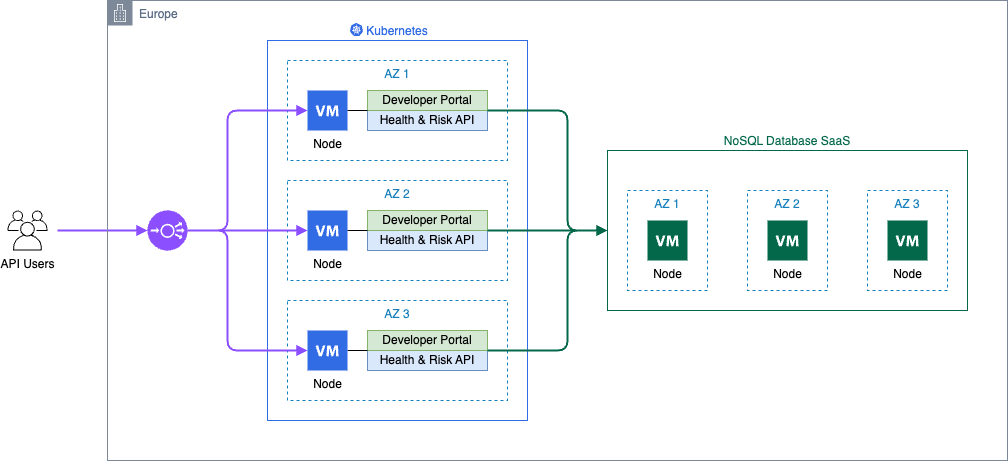
Global and scalable – Multiple global Kubernetes clusters
Operational excellence – Fully serverless and geo-redundant on AWS
Stage 1: Incubation with a virtual machine
After years of scientific research and development, the service was launched, running on a single on-premises virtual machine that used hypervisor technology to provide disaster recovery (DR). However, it had no high availability (HA) capability and it required manual recovery.
The application serving the API requests and the NoSQL database were both running on the same host. Software deployment and operating system maintenance were performed manually using Secure Shell (SSH)—a typical low-automation setup that also included downtime.
The following architecture diagram shows a virtual machine encompassing the monolithic application and its database.
Challenges
A single virtual machine was quick to set up and inexpensive to operate, but it had considerable shortcomings. The health API was only available in Switzerland, infrastructure maintenance was performed manually, and software deployment was handled manually. Additionally, database backups were done using virtual machine snapshots, uptime monitoring only, and testing was conducted on the developer workstation.
Stage 2: Global and scalable with Kubernetes
At that time, dacadoo made a strategic decision to heavily invest in Kubernetes for managing containerized workloads on a global scale. As part of this technology rollout, the health score and risk service were migrated to Kubernetes.
Due to the geographically distributed customer base and low latency requirements, three Kubernetes clusters were deployed, one on each continent. The NoSQL database was hosted in proximity to the workload to reduce service latency and keep the migration effort low.
To reduce the operational maintenance, the NoSQL database was integrated as a SaaS offering, and monitoring was centralized using Datadog.
All cloud infrastructure was provisioned exclusively with Terraform, covering the Kubernetes cluster, NoSQL database , and integration with GitLab and Datadog.
dacadoo containerized the API service and used Gitlab continuous integration and continuous deployment (CI/CD) pipelines to deploy multiple environments and clusters on a global hyperscaler.
In retrospect, this was a typical replatform modernization project from virtual machine to Kubernetes, with a high level of automation and a SaaS-first approach.
The following diagram is the architecture for the container solution with managed NoSQL database.
Challenges
The service faced several challenges, including increased costs from deploying three regional Kubernetes clusters across three environments, resulting in 27 cluster nodes and additional expenses from managing NoSQL database SaaS instances for each cluster. The complexity of CI/CD pipelines for multi-environment multi-cluster deployments added to the difficulty. Significant operational effort was required to keep infrastructure and Kubernetes components up to date.
Stage 3: Operational excellence with serverless
The Kubernetes-based architecture met the requirements, but some features in the dacadoo API service backlog needed to fit better with the application architecture at the time.
This was the right moment to take a holistic view of the infrastructure and software architecture and refactor the solution according to the latest AWS technologies and best practices, the next frontier for dacadoo’s engineering team.
Solution requirements
Requirements for the solution refactoring were as follows:
Keep the functionality of the API unmodified
Constrain data processing to a region of choice for compliance with local data protection laws
Avoid weekly patch cycles by exclusively using managed serverless services
Reduce costs by choosing services with a pay-as-you-go billing model
Delegate authentication to a dedicated service
Use an established web framework with an extensive ecosystem
Refactoring the apps
The API service has two components: a developer portal and the health score and risk calculations API. The database is only required for API keys, algorithm parameters, quotas, and usage statistics. Health data is processed regionally by the compute layer but not persisted, opening the door for a distributed database: Amazon DynamoDB global tables is the perfect fit for the solution. Writes are distributed to all connected Regions, whereas reads are local, providing low latency for complying with dacadoo service level agreements (SLAs).
The developer portal is a web UI with API documentation and API key management features. AWS Lambda is a great fit because it scales automatically and has a pay-per-request billing model.
The health and risk API uses algorithms implemented in the C programming language for short bursting, compute-intense simulations. These calls are wrapped by a REST API using the Python FastAPI framework. These characteristics make AWS Lambda a great fit.
Serverless architecture
HTTP requests are routed to the Lambda functions using Amazon API Gateway with AWS WAF for protection from malicious requests and attacks. Static assets are served from an Amazon Simple Storage Service (Amazon S3) bucket through API Gateway. The additional features of Amazon CloudFront aren’t required, and Amazon S3 reduces the complexity.
Amazon Route 53 provides a powerful feature known as latency-based routing, which allows it to direct DNS queries to the endpoint that offers the lowest latency for the requester.
This feature provides Regional high availability for API users without data processing location requirements. Alternatively, the user can call specific Regional endpoints to make sure requests are processed in the desired Region.
API authorization is HTTP header-based and is performed in the application with data stored in Amazon DynamoDB.
The following diagram is the architecture for a geo-redundant fully serverless solution.
With a dacadoo SRE team proficient in Python, they opted for Pulumi for its advanced features such as programming language flow control constructs, powerful configuration capabilities, and multi-cloud support.
For continuous integration, GitLab CI compiles the algorithm library, tests the FastAPI applications and packages everything. The application deployment is just an update of the AWS Lambda, a simple and reliable workflow.
Summary
The solution evolved from a managed infrastructure setup, where the customer held most of the responsibility, to an AWS managed service architecture.
Infrastructure provisioning evolved from manual, error-prone processes to powerful code-driven workflows in Pulumi. The SRE needed to enhance their software engineering skills to adopt Pulumi, transitioning from configuration-based approaches to designing and maintaining an infrastructure code base using object-oriented Python. This was part of dacadoo’s investment in the SRE team and broader modernization efforts. The serverless architecture enabled a GitOps engineering culture focused on productivity.
The transformation maximized scalability and availability while reducing costs and operational effort:
Virtual machine
Scalability: Low
Availability: Best effort
Infrastructure costs: Low
Maintenance effort: High
Kubernetes
Scalability: High
Availability: 99.95%
Infrastructure costs: High
Maintenance effort: Medium
Serverless
Scalability: Very high
Availability: 99.999% (with failover to another AWS Region)
Infrastructure costs: Low
Maintenance effort: Very low
The global redundancy elevates availability to an impressive 99.999% while keeping the costs low.
Conclusion
Migrating from a virtual machine to Kubernetes and ultimately to AWS Lambda demonstrates the progression of cloud engineering toward enhanced efficiency and scalability.
Each step in this journey reduced the complexity of managing resources while increasing flexibility and automation. Transitioning dacadoo’s API service to a fully serverless, geo-redundant architecture not only advanced the platform but also upskilled engineers, maintained a lean SRE team, and kept infrastructure costs low. Get started with your own AWS serverless solution.
„Дете почина след пушене на вейп.“ „Ученичка почина след три месеца в кома след пушене на „чай“.“
Периодично медиите „избухват“ с подобни заглавия, а държавническата реакция е нещо да се забрани. Дали ще включи в забранителния списък поредното вещество, дали райския газ, дали направо ще се изсили и ще тръгне да забранява самите изпарители (вейпове), реакцията на политическия ни елит винаги е сходна.
Забрани и преследвания
На експертите отдавна е ясно, че бързите и лесни решения рядко са и ефективни. Скоростта, с която организираните групи създават ново сходно вещество, което си е напълно легално, е космическа. И докато държавната машина се задейства, за да забрани едно, на пазара вече има поне два нови негови еквивалента.
Но конкретното е забранено. Политици от всички страни живеят с вярата, че са направили нещо значимо, и… дотам.
Случаи на много млади хора и деца, които загубиха живота си от подобни вещества, има от повече от десет години, а забранените нови психоактивни вещества (синтетични наркотици) в Европа вече са над 1000 различни вида. Лично знам за два случая на деца, жертви на синтетични наркотици, и те нямат нищо общо с работата ми – едното дете почина, другото някак оцеля.
Докато в България се говори основно за синтетични канабиноиди (вещества, които напомнят действието на марихуаната, но са многократно по-силни и по-опасни), успоредно с това в момента се засилва разпространението и търсенето и на синтетични опиати, които напомнят действието на хероина, но са много по-силни и опасни.
Къде грешим?
„Борбата с наркотиците“, както е наречена в законодателството ни, има две основни направления. Първото е намаляване на предлагането – забрани, контрол на митниците, преследване, вкарване в затвора и т.н. Второто е намаляване на търсенето – превенция на употребата, намаляване на вредите от нея, терапия и рехабилитация.
В настоящия период в България се обръща внимание основно на намаляването на предлагането. След всяка подобна трагедия полицията успява да залови някакви количества незаконни вещества, започват дела срещу извършителите. Медиите се успокояват. Политиците се успокояват. Родителите се успокояват.
А месец-два по-късно всичко се повтаря.
Още през 2016 г. на Извънредната асамблея на ООН по темата за наркотиците беше признато, че войната с тях е загубена, както и че е важно да се обърне специално внимание на намаляването на търсенето. А ООН е ригидна структура, която включва в състава си и откровени застъпници на насилието.
Спомням си радостта си от констатацията на ООН. Виждах я като крачка към смисъл, към грижа. Уви, нищо такова не се случи.
Що се отнася до националните стратегии, независимо че в тях са разписани редица смислени мерки, те често просто не се финансират, не се изпълняват или пък откровено се неглижират.
През това време употребата на все по-силни и опасни вещества нараства.
Превенцията
Напоследък доста често говоря с родители за превенцията на употребата на наркотици. Съвсем обяснимо, те са притеснени и задават въпроси, търсейки прост, еднозначен отговор. Обикновено не харесват моя, защото той не е еднозначен.
В обществата с развити системи на превенция тя всъщност е на ниво развитие на личните качества на всяко дете и подобряване на психичното му функциониране. Превенцията е разбиране, топлота и любов. Тя е подкрепата да вземеш по-трудното решение, а именно да не търсиш себеизразяването си чрез наркотични вещества, а да намериш друг начин да си „суперкуул“. Тя е рамото, което ти помага да намериш отдушник на тревогите си, да се научиш как да се справяш с тревожността си, с импулсивността си, с депресивността си, с желанието да „помпаш“ адреналин от силни усещания. Всъщност това са и четирите основни личностни състояния – тревожност, импулсивност, депресивност, търсене на силни усещания, – които могат да доведат и до употреба на наркотици.
Изборът за един млад човек е труден. Във възрастта, в която най-важно е как да бъде приет от приятелите си, как да бъде достатъчно интересен за партньорите си, как да направи впечатление, той трябва да реши да не се възползва от лесния отговор.
Признайте си, че и на вас ви е трудно да не сте конформисти и винаги да постъпвате правилно.
За съжаление, до момента не съм получила обратна връзка от някой от родителите, с които съм разговаряла, че в училищата има смислена и ефективна превенция. Напротив, гледат ме изумено, когато ги попитам какво става там.
Спомням си реакцията на собствения ми племенник, когато преди няколко години сподели, че в училището му е имало посещение от хора, които са говорили по темата. „Лелски, та те ни говориха абсолютни глупости! Всички им се смяха.“ Не знаеше представители на коя институция са били.
Най-широко разпространената в България превенция е т.нар. универсална превенция, т.е. предоставяне на информация. Само по себе си то е полезно, но не води до намаляване на броя на хората, които употребяват наркотични вещества. Ефект имат други видове превенция – селективната и индикативната. При първата се проучва кои са децата, предразположени да потърсят този начин за справяне с ежедневието, и се работи с тях. Втората е насочена към онези, които вече са тръгнали по пътя на употребата на незаконни вещества. А той започва със съвсем законните и напълно достъпни цигари и алкохол.
Вярвам, че е изключително важно да не спираме до децата. Редно е да помислим и за останалите, обикновено млади хора, които започват да употребяват наркотични вещества по-късно. Тук такава мисъл дори не се прокрадва, а проблемът отдавна се вижда с просто око. Студенти, млади хора, излизащи от институции, млади кадри във фирми, не толкова млади компютърни гении…
Намаляване на вредите от употребата на наркотици
Знаете, че има хора, които употребяват наркотици, нали? Познавате някои от тях, но смятате, че те са си окей, те нямат проблем, те са успешни, те ще се справят. Да, в огромната си част това са наши приятели, партньори, лекари, шофьори, адвокати… И те се справят добре, независимо че се забавляват с помощта на един „бонбон“ или пък си почиват с една трева.
Има обаче и едни други хора, родени без шанс, без бъдеще. Хора, които са изтикани от лъскавото ни житие още при раждането си. Някои от тях също употребяват наркотици и също се пристрастяват. Но за тях е още по-трудно да функционират в света на новите технологии, на изкуствения интелект, на електронното банкиране.
Целта на специалистите, които работим в сферата на намаляването на вредите, е да направим всичко необходимо, за да могат онези, които вече употребяват наркотични вещества, да бъдат по-здрави, в по-голяма степен социално приети и по-значими в обществото. Наша работа е да говорим с тях за веществата, за това как да се приемат по по-малко опасен начин. Също да ги подкрепим и да сме до тях по пътя, който ще изминат, докато дойде денят, в който ще поискат промяна. А огромната част от тях ще я поискат. Те няма да се пристрастят и наркотиците ще останат в миналото им.
Друга част няма да се справят сами. Малко по малко ще започнат да губят работата си, апартамента си, приятелите си, семейството… и накрая ще им останем само ние. Много често ще сме единствените, които се интересуват от тях. И това, че са толкова сами, е ужасно тежко, но все пак е нещо, че има къде да отидат. Ние често сме единствената им връзка с „нормалния“ свят, с този, който са загубили и забравили – или пък никога не са имали. Наша работа е да им напомним, че могат да се върнат, че могат да станат част от него. И да ги подкрепим за потърсят лечение, да осигурим нужните документи, да ги заведем на лекар, да им помогнем да си извадят удостоверение от ТЕЛК. Да сме до тях за всички онези неща, които са лесно преодолими за повечето хора, но са непоносимо страшни за човек, загубил всичко в живота си.
Терапия и рехабилитация
Често ми се обаждат хора, които искат бързо разрешаване на проблема. За съжаление, бързо решение няма. Спирането на употребата на наркотици или алкохол е дълъг и много, много труден процес. Когато имаш зависимост, мозъкът ти не работи както при другите хора, трябва му много време да се възстанови. И много търпение от страна на близките, които не разбират през какво преминава човекът, и не проумяват как е възможно да направи огромна крачка напред, а дни по-късно да регресира и да извърши някоя пълна щуротия.
Терапията има много лица, точно както пристрастяването е специфично за всеки отделен човек. И всички начини тя да се извършва трябва да бъдат подкрепени, а човекът да бъде насочен към най-подходящото за него лечение. За някого това може да е психотерапия, за друг – група за взаимопомощ или пък дневен център, вечерни терапевтични групи, терапевтични общности…. Въпрос на добра преценка е всеки да получи помощ по най-бързия и най-подходящ начин.
Тук обаче това рядко се случва.
Тъй като ние работим основно с хора, които са останали без средства и без подкрепа, практиката ни е просто да ги изпращаме към единственото място за професионално безплатно лечение – клиниката в Суходол. Други безплатни варианти могат да са психиатричното отделение в Раднево, групите за самопомощ или някоя религиозна общност. Остава им да се надяват, че са извадили късмет и са на правилното място, а близките им да стискат палци, че това ще сработи.
За зависимите, които или чиито близки все още разполагат с финансови възможности, са налични и някои добре работещи частни терапевтични програми. Казвам „някои“, защото има и откровени шмекери, които продават надежда, но не могат да лекуват ефективно. Свидетели сме как лечението на зависимости често се разглежда като доходоносен бизнес. Тоест ако попаднете в някоя от тези програми, ще бъдете приети, посрещнати на червен килим и уверявани, че това е най-доброто място за терапия. Понякога може да е така, понякога – не.
Уви, такива са възможностите тук. И с тях трябва да успяваме да спасяваме близките си, докато се надяваме държавата, т.е. политиците ни да започнат да вършат работата си и да подобрят цялата система.
А кога това ще стане, е труден въпрос. Защото просто темата не е „секси“ политически.
With Take Command 2025 just around the corner, we sat down with Raj Samani, Chief Scientist at Rapid7, for a preview of his upcoming session: Inside the Mind of an Attacker: Navigating the Threat Horizon.
Raj will be joined by Trent Teyema, Founder and President at CSG Strategies and former head of the FBI Cyber Division, and moderator Brian Honan, CEO of BH Consulting. Together, they bring decades of experience across cyber intelligence, national security, and frontline incident response.
So what can attendees expect from the session, and the day as a whole?
A Panel Built for Practical Impact
“This isn’t a talking shop,” Raj told us. “The people on this panel are practitioners. They do the job.”
Rather than focus on theory, the session aims to provide clear, actionable guidance rooted in real-world expertise. Raj describes the panel as a rare convergence of perspectives: vendors developing the tools, consultants advising organizations directly, and former government leaders who’ve pursued and prosecuted threat actors.
“We’ve got three legs of the solution represented,” he said. “And the audience is the fourth. Between us, we’re covering every side of the response equation.”
The Shift in Attacker Capabilities
While Raj didn’t give away too much ahead of the session, he offered a clear warning: attacker capabilities have evolved—rapidly.
“In the past, tools and techniques used by advanced nation-state actors were out of reach for most criminals,” he explained. “Now, even relatively inexperienced threat actors have access to those same capabilities. That changes everything.”
Organizations today face a constant flood of vulnerabilities, alerts, and data to prioritize – often without the context needed to make effective decisions.
“It’s not that we have a data problem,” Raj noted. “It’s that we have a context problem. We’re overwhelmed, and the inability to act quickly and decisively is putting organizations at risk.”
That’s where visibility and prioritization come into play—two capabilities central to Exposure Management and solutions like Rapid7’s Exposure Command.
Why This Session Matters
Raj emphasized that this session is about helping practitioners walk away with tangible answers to critical questions:
How do I know if I’ve been compromised?
Are adversaries still in my network?
Which vulnerabilities actually matter?
What can I do to reduce risk—today?
“These are the questions every security leader needs to be able to answer. Because if you can’t, how long will your executive team trust you to lead the charge?”
Why Attend Take Command 2025?
Raj was clear: this isn’t just another virtual event.
“Take Command is one of our most important moments of the year,” he told us. “It’s where we bring everything together, sharing the latest research, strategies, experiences and innovations from those on the front lines.and give people the chance to hear what’s actually happening on the front lines.”
He also noted that sessions like his don’t come around often, making this a rare opportunity to hear directly from experts working across national security, threat intelligence, and hands-on incident response.
Don’t Miss It
Take Command 2025 takes place April 9, 2025, and features a full day of virtual sessions covering AI, MDR, threat intelligence, red teaming, and more.
Raj Samani’s panel, “Inside the Mind of an Attacker,” is one you won’t want to miss.
To provide the best experiences, we use technologies like cookies to store and/or access device information. Consenting to these technologies will allow us to process data such as browsing behavior or unique IDs on this site. Not consenting or withdrawing consent, may adversely affect certain features and functions.
Functional
Always active
The technical storage or access is strictly necessary for the legitimate purpose of enabling the use of a specific service explicitly requested by the subscriber or user, or for the sole purpose of carrying out the transmission of a communication over an electronic communications network.
Preferences
The technical storage or access is necessary for the legitimate purpose of storing preferences that are not requested by the subscriber or user.
Statistics
The technical storage or access that is used exclusively for statistical purposes.The technical storage or access that is used exclusively for anonymous statistical purposes. Without a subpoena, voluntary compliance on the part of your Internet Service Provider, or additional records from a third party, information stored or retrieved for this purpose alone cannot usually be used to identify you.
Marketing
The technical storage or access is required to create user profiles to send advertising, or to track the user on a website or across several websites for similar marketing purposes.